Post Syndicated from BeardedTinker original https://www.youtube.com/watch?v=IVTNiW1H6oc
Как думата „мигрант“ стана дехуманизираща
Post Syndicated from Светла Енчева original https://www.toest.bg/kak-dumata-migrant-stana-dehumanizirashta/

С наближаването на европейските избори някои политически сили се нуждаят от враг, за да мобилизират избирателите си. От внезапно изникналата без реално основание ксенофобска истерия в началото на март тази година може да се предположи, че основният набелязан враг за предстоящата предизборна кампания ще са чужденците. За да разберем как се създава определено отношение към дадена група хора, е важно да разбираме какъв език се прилага спрямо тази група.
По какво си приличат думите „мигрант“ и „джендър“? И в двата случая те масово се използват в смисъл, различен от този, който експертите в съответните области влагат в тях. И в двата случая превратните употреби на термините са дехуманизиращи за определени групи хора. Но докато манипулативният смисъл на „джендър“ е ограничен в определени държави, религиозни общности и политически кръгове, този на „мигрант“ е придобил по-широка популярност.
Ето защо, когато неотдавна българските медии съобщиха, че чужденците в общежитието на Държавната агенция за бежанците (ДАБ) в квартал „Овча купел“ са мигранти, а нападнатите чуждестранни студенти в село Храбрино и на столичния булевард „Витоша“ не са, изглеждаше ясно за какво става дума. Абсурда видяха комай само онези, които разбират от миграционни изследвания.
Какво казват теориите за миграцията?
„Миграционни изследвания“ е интердисциплинарна академична област. Тя съдържа елементи от социологията, статистиката, демографията, географията, историята, правото и др. Съществуват различни теории за същността на миграцията. В книгата си „От миграция към мобилност. Политики и пътища“ проф. Анна Кръстева, международно призната експертка в областта, пише: „Най-разпространеното определение за миграцията е движение на хора извън границите на страната за повече от една година [курсивът мой – б.а.].“
Кръстева обръща внимание на множеството форми на миграция. Има и циклична миграция – например на сезонните работници или на пътуващите за известни периоди при роднини или интимни партньори и др. Според нея миграцията дълго време се е мислила като „стрелки“ – промяна на мястото на пребиваване веднъж и завинаги, докато тя все повече прилича на „спагети“ – тоест хората заминават, връщат се или се заселват на нови места.
Хората, които мигрират, са мигранти. Мигранти са и над един милион българи, заселили се в чужди държави, както и българските сезонни работници в чужбина. Проф. Марина Лякова, която преподава миграционни изследвания в Германия, прави мащабно изследване на трите основни периода на миграция на българите в тази страна от началото на социализма до наши дни. То е публикувано в книгата ѝ „Възпирана, прикрита, невидима. Миграция и мобилност от България към Германия“ (на немски език).
Миграция и мобилност са различни неща. Туризмът, командировките и краткосрочните специализации са форми на мобилност, не на миграция. Затова се говори за „мобилност на учените“, а не за „миграция на учените“.
И какво излиза? Според най-разпространените миграционни теории чуждестранните студенти са мигранти, защото следването им продължава няколко години. А чужденците, залавяни на българо-турската граница или във вътрешността на страната, както и повечето от обитателите на общежитията на ДАБ не са мигранти, защото са в страната по-малко от една година.
По отношение на хората, които бягат от родните си страни, се използват най-общо определенията „бежанци“ и „търсещи убежище“. Търсещите убежище са онези, които кандидатстват за легален статут, докато думата „бежанци“ се използва за онези, които вече са получили статут, но често включва и търсещите убежище. Юридически обаче термините „статут на бежанец“ или „статут на убежище“ означават доста по-конкретни неща, освен това съществуват и други названия за хората, търсещи спасение в друга държава.
Какво казва българското законодателство?
Две основни институции регулират статута на чужденците в България. Това са ДАБ и Дирекция „Миграция“ на МВР. ДАБ решава на кого да се даде (или да не се даде) убежище, и предоставя подслон на онези, които изчакват решението ѝ и нямат средства да се издържат сами. Дирекция „Миграция“ урежда (или отказва да уреди) статута на пребиваване на чужденци, дошли в България, за да работят, учат, да се съберат със семействата си и т.н. И депортира (или затваря в центрове за задържане) чужденци без легален статут.
Няколко закона уреждат престоя на чужденци в България, като най-важните от тях са Законът за убежището и бежанците, Законът за чужденците в Република България и Законът за влизането, пребиваването и напускането на Република България на гражданите на Европейския съюз и членовете на техните семейства. В нито един от тях не присъства думата „мигрант“.
Нека се спрем по-подробно върху Закона за убежището и бежанците (ЗУБ), защото той се отнася до онези чужденци, които масово се асоциират с „мигранти“. По силата на този закон България предоставя на чужденци три типа закрила – убежище, международна закрила и временна закрила.
ЗУБ се позовава на Конституцията, че статут на убежище предоставя президентът. Президентската институция пък делегира това право на вицепрезидента, към когото е сформирана Комисия по предоставяне на убежище. Трудно можем да се сетим за случай, в който вицепрезидентът да се е възползвал от това си право и въпросната комисия да е свършила нещо.
Останалите видове закрила са в компетенциите на ДАБ. Международната закрила включва статут на бежанец и хуманитарен статут. Статутът на бежанец е за чужденци, които имат основания да се опасяват от преследване (например заради политическите си възгледи, религията или националността). Хуманитарният статут е предназначен за лица, които не отговарят на условията за бежанци, но все пак животът им е под заплаха – поради войни, конфликти или други причини от хуманитарен характер.
За разлика от международната закрила, която се предоставя или отказва за всеки отделен случай, временната закрила се отнася за цяла група хора. Принадлежността към съответната група е достатъчно основание за получаване на статут. Единственият случай на предоставяне на временна закрила в България е този с украинските бежанци.
Кой е легален и кой не е?
Отразявайки случаите, използвани за провокиране на ксенофобски настроения в началото на март, някои медии представиха чуждестранните студенти като „легално“ пребиваващи, за разлика от търсещите убежище в общежитието на ДАБ. Ала и едните, и другите са в България легално. Как тогава се стига до подобни внушения?
Институциите (най-вече МВР) често наричат търсещите убежище „незаконно“ или „нелегално пресекли границата“. Този език се използва и от политици, възприема се и от медиите. Така се създава впечатлението, че тези хора пребивават в България без правно основание и са, както е разпространено да се казва, „нелегални мигранти“. Вече стана ясно, че те не са мигранти в класическия смисъл на думата, но всъщност и нелегални не са. Защо?
Ако един чужденец премине границата без разрешение, но поиска убежище, след като се предаде на властите или е заловен от тях, ДАБ трябва да започне производство за предоставянето на някой от описаните по-горе видове статут за този човек. Докато очаква ДАБ да се произнесе, чужденецът пребивава легално. В общежитията на ДАБ (като това в „Овча купел“) са настанени точно такива хора.
Незаконното преминаване на границата е най-разпространеният начин човек да потърси убежище, а за бягащите от много държави и конфликтни райони е и единственият възможен. Никой няма да им даде виза, за да избягат. И в този случай единственото изключение, което българската държава (и ЕС) прави, е за украинските бежанци. По време на т.нар. Възродителен процес пък Турция временно отваря границите си за депортираните от България около 300 000 етнически турци.
Дори ако кандидатстващите за статут получат отказ, те могат да решат да обжалват или пък да започнат ново производство, прилагайки нови обстоятелства към своя случай – като Оксана и Елена от Русия, с които разговаря „Тоест“. Или да кандидатстват за убежище пред президента. В тези случаи престоят им в страната продължава да е законен.
Едва ако всички варианти са изчерпани, търсещият убежище може да се окаже без легален статут. Без статут впрочем може да останат и чужденци, дошли в България на друго основание, например работа, образование или брак. Това е възможно да се случи, ако например основанието им за пребиваване престане да е валидно или ако не си подновят документите навреме.
Как се промени значението на думата „мигрант“?
Някъде до 2015–2016 г. думата „мигрант“ не се използваше в настоящия си смисъл на „бежанец“ или „нелегално пребиваващ чужденец“, а се употребяваше най-вече в експертни кръгове. В България бежанците и търсещите убежище бяха наричани или „бежанци“, или неправилно „нелегални имигранти“, или още по-неправилно – „нелегални емигранти“. Имигрантите са чужденци, които се заселват в една държава не защото бягат, а по други причини, а емигрантите са представители на местното население, които напускат страната си, за да се заселят другаде.
Промяната на значението на думата „мигрант“ в публичния език настъпи в контекста на т.нар. криза с търсещите убежище през 2015 г. Мнозинството от тях бягаха от Сирия заради кървавите конфликти в тази страна, имаше и бягащи от Афганистан, както и от други страни.
Първоначално не се говореше за мигрантска криза, а за „бежанска вълна“, „бежанска криза“, „наплив на бежанци“, „бежанско бреме“. От онзи период е и известният лозунг Refugees welcome („Добре дошли, бежанци“). Постепенно думата „бежанци“ започна да се измества от „мигранти“, а кризата от бежанска стана „мигрантска криза“.
Роля за тази промяна изиграха не само някои европейски политици и гласове, критично настроени към търсещите убежище, а и политиката в САЩ и американски медии като Reuters, пишещи за Европа, чиито новини масово се превеждат от българските медии. Промяната всъщност съвпадна с политическия възход на Доналд Тръмп, който спечели изборите за президент на САЩ в края на 2016 г. Неговата реторика се характеризира с ксенофобски патос, а едно от основните му предизборни обещания, което той отчасти изпълни, беше изграждането на стена по границата с Мексико.
„Мигранти“ от Близкия изток и Африка, но „украински бежанци“
Замяната на определенията „бежанци“ и „търсещи убежище“ с „мигранти“ на пръв поглед е неутрална, каквото е и самото понятие. Обаче тази неутралност се оказва привидна. Когато говорим за бежанци, е ясно, че имаме предвид хора, които бягат от нещо. По същия начин търсещите убежище са загубени без това убежище.
Думата „мигранти“ обаче няма такива конотации – човек може да мигрира по всякакви причини. С употребата ѝ по адрес на хора, които бягат от война, конфликти или преследване, се създава впечатлението, че те всъщност нямат основателна причина да бягат. Така се налива масло в ксенофобския дискурс, че тези хора нахлуват неканени в европейските страни, за да затрудняват социалните им системи и да бъдат заплаха за местното население.
В определянето на бежанците като „мигранти“ има и скрит расизъм. В този си нов смисъл думата „мигранти“ се асоциира предимно с бежанци от Близкия изток и Африка, повечето от които са с цвят на кожата, различен от бял. Много от тях идват от страни, в които ислямът е доминиращата религия. Накратко, те се отличават от местното европейско население по външен вид и по култура.
Замисляли ли сте се защо украинските бежанци са наричани именно бежанци, а не „украински мигранти“? Със самия израз се предпоставя, че те имат основателна причина да избягат от страната си и заслужават да им се даде убежище. За разлика от бежанците от Близкия изток и Африка, повечето украинци са със светъл цвят на кожата. Преобладаващата религия в страната е християнството. Те са близки до европейците както по външен вид, така и по култура.
Езикът, който неусетно дехуманизира
Важно е как използваме думите, защото чрез тях възприемаме света. Австрийският философ Лудвиг Витгенщайн казва, че границите на езика ни означават границите на света ни. Ако възприемаме бягащите от преследване, войни и конфликти като „мигранти“, които влизат в страната „незаконно“, е малко вероятно да им дадем убежище и да ги приемем в обществото си. Наричайки ги по този начин, ние предпоставяме, че те не са толкова ценни като хора, колкото сме ние, и ни е безразлично дали ще оцелеят.
Това е форма на дехуманизация. Журналистката Татяна Ваксберг определя дехуманизацията като „представянето на група хора не като сбор от индивиди, а като аморфна маса, несъвместима с обичайните човешки черти и неспособна на човешки чувства“. Тя предупреждава, че дехуманизацията е последният етап преди физическата разправа с тази група. Спрямо търсещите убежище в България от Близкия изток физическата саморазправа е разпространена практика – като се почне от отношението на границата, където много от тях са бити, ограбвани и връщани насила в Турция от граничари.
Тук трябва да се отбележи, че България е външна граница на ЕС и иска да бъде пълноправен член на Шенгенското пространство, а ЕС трудно може да приеме всички, които искат да се спасят в него. Затова поставя условие пред България да ограничи „мигрантския натиск“. Това обяснява както преминаването към привидно неутралния дискурс за „мигрантите“, така и насилието по границите ни, масовите откази за предоставяне на статут, нехуманното отношение към бежанци, затворени в центрове като този в Бусманци.
Тъй като обаче става дума за хора, ограничаването на достъпа им до убежище следва да е свързано с осъзнаване на моралната цена, която се плаща. Затова говоренето за бежанците и търсещите убежище като за „мигранти“ е опасно – то не само е неграмотно от академична гледна точка, а и приспива моралните ни сетива.
Scale AWS Glue jobs by optimizing IP address consumption and expanding network capacity using a private NAT gateway
Post Syndicated from Sushanth Kothapally original https://aws.amazon.com/blogs/big-data/scale-aws-glue-jobs-by-optimizing-ip-address-consumption-and-expanding-network-capacity-using-a-private-nat-gateway/
As businesses expand, the demand for IP addresses within the corporate network often exceeds the supply. An organization’s network is often designed with some anticipation of future requirements, but as enterprises evolve, their information technology (IT) needs surpass the previously designed network. Companies may find themselves challenged to manage the limited pool of IP addresses.
For data engineering workloads when AWS Glue is used in such a constrained network configuration, your team may sometimes face hurdles running many jobs simultaneously. This happens because you may not have enough IP addresses to support the required connections to databases. To overcome this shortage, the team may get more IP addresses from your corporate network pool. These obtained IP addresses can be unique (non-overlapping) or overlapping, when the IP addresses are reused in your corporate network.
When you use overlapping IP addresses, you need an additional network management to establish connectivity. Networking solutions can include options like private Network Address Translation (NAT) gateways, AWS PrivateLink, or self-managed NAT appliances to translate IP addresses.
In this post, we will discuss two strategies to scale AWS Glue jobs:
- Optimizing the IP address consumption by right-sizing Data Processing Units (DPUs), using the Auto Scaling feature of AWS Glue, and fine-tuning of the jobs.
- Expanding the network capacity using additional non-routable Classless Inter-Domain Routing (CIDR) range with a private NAT gateway.
Before we dive deep into these solutions, let us understand how AWS Glue uses Elastic Network Interface (ENI) for establishing connectivity. To enable access to data stores inside a VPC, you need to create an AWS Glue connection that is attached to your VPC. When an AWS Glue job runs in your VPC, the job creates an ENI inside the configured VPC for each data connection, and that ENI uses an IP address in the specified VPC. These ENIs are short-lived and active until job is complete.
Now let us look at the first solution that explains optimizing the AWS Glue IP address consumption.
Strategies for efficient IP address consumption
In AWS Glue, the number of workers a job uses determines the count of IP addresses used from your VPC subnet. This is because each worker requires one IP address that maps to one ENI. When you don’t have enough CIDR range allocated to the AWS Glue subnet, you may observe IP address exhaustion errors. The following are some best practices to optimize AWS Glue IP address consumption:
- Right-sizing the job’s DPUs – AWS Glue is a distributed processing engine. It works efficiently when it can run tasks in parallel. If a job has more than the required DPUs, it doesn’t always run quicker. So, finding the right number of DPUs will make sure you use IP addresses optimally. By building observability in the system and analyzing the job performance, you can get insights into ENI consumption trends and then configure the appropriate capacity on the job for the right size. For more details, refer to Monitoring for DPU capacity planning. The Spark UI is a helpful tool to monitor AWS Glue jobs’ workers usage. For more details, refer to Monitoring jobs using the Apache Spark web UI.
- AWS Glue Auto Scaling – It’s often difficult to predict a job’s capacity requirements upfront. Enabling the Auto Scaling feature of AWS Glue will offload some of this responsibility to AWS. At runtime based on the workload requirements, the job automatically scales worker nodes upto the defined maximum configuration. If there is no additional need, AWS Glue will not overprovision workers, thereby saving resources and reducing cost. The Auto Scaling feature is available in AWS Glue 3.0 and later. For more information, refer to Introducing AWS Glue Auto Scaling: Automatically resize serverless computing resources for lower cost with optimized Apache Spark.
- Job-level optimization – Identify job-level optimizations by using AWS Glue job metrics , and apply best practices from Best practices for performance tuning AWS Glue for Apache Spark jobs.
Next let us look at the second solution that elaborates network capacity expansion.
Solutions for network size (IP address) expansion
In this section, we will discuss two possible solutions to expand network size in more detail.
Expand VPC CIDR ranges with routable addresses
One solution is to add more private IPv4 CIDR ranges from RFC 1918 to your VPC. Theoretically, each AWS account can be assigned to some or all these IP address CIDRs. Your IP Address Management (IPAM) team often manages the allocation of IP addresses that each business unit can use from RFC1918 to avoid overlapping IP addresses across multiple AWS accounts or business units. If your current routable IP address quota allocated by the IPAM team is not sufficient, then you can request for more.
If your IPAM team issues you an additional non-overlapping CIDR range, then you can either add it as a secondary CIDR to your existing VPC or create a new VPC with it. If you are planning to create a new VPC, then you can inter-connect the VPCs via VPC peering or AWS Transit Gateway.
If this additional capacity is sufficient to run all your jobs within defined the timeframe, then it is a simple and cost-effective solution. Otherwise, you can consider adopting overlapping IP addresses with a private NAT gateway, as described in the following section. With the following solution you must use Transit Gateway to connect VPCs as VPC peering is not possible when there are overlapping CIDR ranges in those two VPCs.
Configure non-routable CIDR with a private NAT gateway
As described in the AWS whitepaper Building a Scalable and Secure Multi-VPC AWS Network Infrastructure, you can expand your network capacity by creating a non-routable IP address subnet and using a private NAT gateway that is located in a routable IP address space (non-overlapping) to route traffic. A private NAT gateway translates and routes traffic between non-routable IP addresses and routable IP addresses. The following diagram demonstrates the solution with reference to AWS Glue.

As you can see in the above diagram, VPC A (ETL) has two CIDR ranges attached. The smaller CIDR range 172.33.0.0/24 is routable because it not reused anywhere, whereas the larger CIDR range 100.64.0.0/16 is non-routable because it is reused in the database VPC.
In VPC B (Database), we have hosted two databases in routable subnets 172.30.0.0/26 and 172.30.0.64/26. These two subnets are in two separate Availability Zones for high availability. We also have two additional unused subnet 100.64.0.0/24 and 100.64.1.0/24 to simulate a non-routable setup.
You can choose the size of the non-routable CIDR range based on your capacity requirements. Since you can reuse IP addresses, you can create a very large subnet as needed. For example, a CIDR mask of /16 would give you approximately 65,000 IPv4 addresses. You can work with your network engineering team and size the subnets.
In short, you can configure AWS Glue jobs to use both routable and non-routable subnets in your VPC to maximize the available IP address pool.
Now let us understand how Glue ENIs that are in a non-routable subnet communicate with data sources in another VPC.

The data flow for the use case demonstrated here is as follows (referring to the numbered steps in figure above):
- When an AWS Glue job needs to access a data source, it first uses the AWS Glue connection on the job and creates the ENIs in the non-routable subnet 100.64.0.0/24 in VPC A. Later AWS Glue uses the database connection configuration and attempts to connect to the database in VPC B 172.30.0.0/24.
- As per the route table
VPCA-Non-Routable-RouteTablethe destination 172.30.0.0/24 is configured for a private NAT gateway. The request is sent to the NAT gateway, which then translates the source IP address from a non-routable IP address to a routable IP address. Traffic is then sent to the transit gateway attachment in VPC A because it’s associated with theVPCA-Routable-RouteTableroute table in VPC A. - Transit Gateway uses the 172.30.0.0/24 route and sends the traffic to the VPC B transit gateway attachment.
- The transit gateway ENI in VPC B uses VPC B’s local route to connect to the database endpoint and query the data.
- When the query is complete, the response is sent back to VPC A. The response traffic is routed to the transit gateway attachment in VPC B, then Transit Gateway uses the 172.33.0.0/24 route and sends traffic to the VPC A transit gateway attachment.
- The transit gateway ENI in VPC A uses the local route to forward the traffic to the private NAT gateway, which translates the destination IP address to that of ENIs in non-routable subnet.
- Finally, the AWS Glue job receives the data and continues processing.
The private NAT gateway solution is an option if you need extra IP addresses when you can’t obtain them from a routable network in your organization. Sometimes with each additional service there is an additional cost incurred, and this trade-off is necessary to meet your goals. Refer to the NAT Gateway pricing section on the Amazon VPC pricing page for more information.
Prerequisites
To complete the walk-through of the private NAT gateway solution, you need the following:
- An AWS account with a role that has sufficient access to provision the required resources.
- An AWS Identity and Access Management (IAM) user with access to AWS resources, including Amazon Virtual Private Cloud (Amazon VPC), Transit Gateway, a private NAT gateway, and an Amazon Relational Database Service (Amazon RDS) for MySQL database.
Deploy the solution
To implement the solution, complete the following steps:
- Sign in to your AWS management console.
- Deploy the solution by clicking
 . This stack defaults to
us-east-1, you can select your desired Region. - Click next and then specify the stack details. You can retain the input parameters to the prepopulated default values or change them as needed.
- For
DatabaseUserPassword, enter an alphanumeric password of your choice and ensure to note it down for further use. - For
S3BucketName, enter a unique Amazon Simple Storage Service (Amazon S3) bucket name. This bucket stores the AWS Glue job script that will be copied from an AWS public code repository.
- Click next.
- Leave the default values and click next again.
- Review the details, acknowledge the creation of IAM resources, and click submit to start the deployment.


You can monitor the events to see resources being created on the AWS CloudFormation console. It may take around 20 minutes for the stack resources to be created.
After the stack creation is complete, go to the Outputs tab on the AWS CloudFormation console and note the following values for later use:
DBSourceDBTargetSourceCrawlerTargetCrawler
Connect to an AWS Cloud9 instance
Next, we need to prepare the source and target Amazon RDS for MySQL tables using an AWS Cloud9 instance. Complete the following steps:
- On the AWS Cloud9 console page, locate the
aws-glue-cloud9environment. - In the Cloud9 IDE column, click on Open to launch your AWS Cloud9 instance in a new web browser.
Prepare the source MySQL table
Complete the following steps to prepare your source table:
- From the AWS Cloud9 terminal, install the MySQL client using the following command:
sudo yum update -y && sudo yum install -y mysql - Connect to the source database using the following command. Replace the source hostname with the DBSource value you captured earlier. When prompted, enter the database password that you specified during the stack creation.
mysql -h <Source Hostname> -P 3306 -u admin -p - Run the following scripts to create the source
emptable, and load the test data:-- connect to source database USE srcdb; -- Drop emp table if it exists DROP TABLE IF EXISTS emp; -- Create the emp table CREATE TABLE emp (empid INT AUTO_INCREMENT, ename VARCHAR(100) NOT NULL, edept VARCHAR(100) NOT NULL, PRIMARY KEY (empid)); -- Create a stored procedure to load sample records into emp table DELIMITER $$ CREATE PROCEDURE sp_load_emp_source_data() BEGIN DECLARE empid INT; DECLARE ename VARCHAR(100); DECLARE edept VARCHAR(50); DECLARE cnt INT DEFAULT 1; -- Initialize counter to 1 to auto-increment the PK DECLARE rec_count INT DEFAULT 1000; -- Initialize sample records counter TRUNCATE TABLE emp; -- Truncate the emp table WHILE cnt <= rec_count DO -- Loop and load the required number of sample records SET ename = CONCAT('Employee_', FLOOR(RAND() * 100) + 1); -- Generate random employee name SET edept = CONCAT('Dept_', FLOOR(RAND() * 100) + 1); -- Generate random employee department -- Insert record with auto-incrementing empid INSERT INTO emp (ename, edept) VALUES (ename, edept); -- Increment counter for next record SET cnt = cnt + 1; END WHILE; COMMIT; END$$ DELIMITER ; -- Call the above stored procedure to load sample records into emp table CALL sp_load_emp_source_data(); - Check the source
emptable’s count using the below SQL query (you need this at later step for verification).select count(*) from emp; - Run the following command to exit from the MySQL client utility and return to the AWS Cloud9 instance’s terminal:
quit;
Prepare the target MySQL table
Complete the following steps to prepare the target table:
- Connect to the target database using the following command. Replace the target hostname with the DBTarget value you captured earlier. When prompted enter the database password that you specified during the stack creation.
mysql -h <Target Hostname> -P 3306 -u admin -p - Run the following scripts to create the target
emptable. This table will be loaded by the AWS Glue job in the subsequent step.-- connect to the target database USE targetdb; -- Drop emp table if it exists DROP TABLE IF EXISTS emp; -- Create the emp table CREATE TABLE emp (empid INT AUTO_INCREMENT, ename VARCHAR(100) NOT NULL, edept VARCHAR(100) NOT NULL, PRIMARY KEY (empid) );
Verify the networking setup (Optional)
The following steps are useful to understand NAT gateway, route tables, and the transit gateway configurations of private NAT gateway solution. These components were created during the CloudFormation stack creation.
- On the Amazon VPC console page, navigate to Virtual private cloud section and locate NAT gateways.
- Search for NAT Gateway with name
Glue-OverlappingCIDR-NATGWand explore it further. As you can see in the following screenshot, the NAT gateway was created in VPC A (ETL) on the routable subnet.
- In the left side navigation pane, navigate to Route tables under virtual private cloud section.
- Search for
VPCA-Non-Routable-RouteTableand explore it further. You can see that the route table is configured to translate traffic from overlapping CIDR using the NAT gateway.
- In the left side navigation pane, navigate to Transit gateways section and click on Transit gateway attachments. Enter
VPC-in the search box and locate the two newly created transit gateway attachments. - You can explore these attachments further to learn their configurations.


Run the AWS Glue crawlers
Complete the following steps to run the AWS Glue crawlers that are required to catalog the source and target emp tables. This is a prerequisite step for running the AWS Glue job.
- On the AWS Glue Console page, under Data Catalog section in the navigation pane, click on Crawlers.
- Locate the source and target crawlers that you noted earlier.
- Select these crawlers and click Run to create the respective AWS Glue Data Catalog tables.
- You can monitor the AWS Glue crawlers for the successful completion. It may take around 3–4 minutes for both crawlers to complete. When they’re done, the last run status of the job changes to Succeeded, and you can also see there are two AWS Glue catalog tables created from this run.


Run the AWS Glue ETL job
After you set up the tables and complete the prerequisite steps, you are now ready to run the AWS Glue job that you created using the CloudFormation template. This job connects to the source RDS for MySQL database, extracts the data, and loads the data into the target RDS for MySQL database. This job reads data from a source MySQL table and loads it to the target MySQL table using private NAT gateway solution. To run the AWS Glue job, complete the following steps:
- On the AWS Glue console, click on ETL jobs in the navigation pane.
- Click on the job
glue-private-nat-job. - Click Run to start it.
The following is the PySpark script for this ETL job:
import sys
from awsglue.transforms import *
from awsglue.utils import getResolvedOptions
from pyspark.context import SparkContext
from awsglue.context import GlueContext
from awsglue.job import Job

args = getResolvedOptions(sys.argv, ["JOB_NAME"])
sc = SparkContext()
glueContext = GlueContext(sc)
spark = glueContext.spark_session
job = Job(glueContext)
job.init(args["JOB_NAME"], args)

# Script generated for node AWS Glue Data Catalog
AWSGlueDataCatalog_node = glueContext.create_dynamic_frame.from_catalog(
    database="glue_cat_db_source",
    table_name="srcdb_emp",
    transformation_ctx="AWSGlueDataCatalog_node",
)

# Script generated for node Change Schema
ChangeSchema_node = ApplyMapping.apply(
    frame=AWSGlueDataCatalog_node,
    mappings=[
        ("empid", "int", "empid", "int"),
        ("ename", "string", "ename", "string"),
        ("edept", "string", "edept", "string"),
    ],
    transformation_ctx="ChangeSchema_node",
)

# Script generated for node AWS Glue Data Catalog
AWSGlueDataCatalog_node = glueContext.write_dynamic_frame.from_catalog(
    frame=ChangeSchema_node,
    database="glue_cat_db_target",
    table_name="targetdb_emp",
    transformation_ctx="AWSGlueDataCatalog_node",
)

job.commit()
Based on the job’s DPU configuration, AWS Glue creates a set of ENIs in the non-routable subnet that is configured on the AWS Glue connection. You can monitor these ENIs on the Network Interfaces page of the Amazon Elastic Compute Cloud (Amazon EC2) console.
The below screenshot shows the 10 ENIs that were created for the job run to match the requested number of workers configured on the job parameters. As expected, the ENIs were created in the non-routable subnet of VPC A, enabling scalability of IP addresses. After the job is complete, these ENIs will be automatically released by AWS Glue.
When the AWS Glue job is running, you can monitor its status. Upon successful completion, the job’s status changes to Succeeded.
Verify the results
After the AWS Glue job is complete, connect to the target MySQL database. Verify if the target record count matches to the source. You can use the below SQL query in AWS Cloud9 terminal.
USE targetdb;
SELECT count(*) from emp;
Finally, exit from the MySQL client utility using the following command and return to the AWS Cloud9 terminal: quit;
You can now confirm that AWS Glue has successfully completed a job to load data to a target database using the IP addresses from a non-routable subnet. This concludes end to end testing of the private NAT gateway solution.
Clean up
To avoid incurring future charges, delete the resource created via CloudFormation stack by completing the following steps:
- On the AWS CloudFormation console, click Stacks in the navigation pane.
- Select the stack
AWSGluePrivateNATStack. - Click on Delete to delete the stack. When prompted confirm the stack deletion.
Conclusion
In this post, we demonstrated how you can scale AWS Glue jobs by optimizing IP addresses consumption and expanding your network capacity by using a private NAT gateway solution. This two-fold approach helps you to get unblocked in an environment that has IP address capacity constraints. The options discussed in the AWS Glue IP address optimization section are complimentary to the IP address expansion solutions, and you can iteratively build to mature your data platform.
Learn more about AWS Glue job optimization techniques from Monitor and optimize cost on AWS Glue for Apache Spark and Best practices to scale Apache Spark jobs and partition data with AWS Glue.
About the authors
 Sushanth Kothapally is a Solutions Architect at Amazon Web Services supporting Automotive and Manufacturing customers. He is passionate about designing technology solutions to meet business goals and has keen interest in serverless and event-driven architectures.
 Senthil Kamala Rathinam is a Solutions Architect at Amazon Web Services specializing in Data and Analytics. He is passionate about helping customers to design and build modern data platforms. In his free time, Senthil loves to spend time with his family and play badminton.
Малайзия по стените
Post Syndicated from Петя Кокудева original https://www.toest.bg/malayziya-po-stenitie/
<< Към първа част
Не съм била в друга страна по света, където можеш да научиш толкова много за бита и ежедневието на хората от… уличните рисунки.

Почти всеки голям град има улица или периметър от няколко улички, чиито стени са изрисувани. Това обаче не са обичайните графити. Тук те изграждат една цялостна и много детайлна галерия на малайското ежедневие. Някои стени представят ритуалите на пиене на кафе и чай, като например те тарик – емблематичния им чай с подсладено мляко, който се прелива няколко пъти между две чаши, за да поизстине. Понякога преливането е от цял метър височина и има майстори в тази работа. Други рисунки изобразяват традиционни ястия, като наси лемак – завит в голямо бананово листо ориз, варен в кокосово мляко и гарниран с аншоа, пържени ядки и лют сос.


© Изрисувани стени в различни градове
Има и стени, които ви отвеждат сред суматохата на типичните за Малайзия нощни пазари, откъдето може да си купите керопок лекор – нещо като рибен чипс. А други функционират като разговорник и ще ви научат на основни фрази: терима каси – „благодаря“; апа кабар – „как си“; минта мааф – „съжалявам“.

Ръцете на танцьорката
Има обаче и по-живописни от градските стени – това са типичните кампунг къщи. Успях да видя най-различни благодарение на това, че направихме пълно завъртане из страната – близо 3000 километра.
Малайската къща е дървена, повдигната на поне метър-два над земята (заради честите наводнения) и с изящно гравирана фасада. Тукашната дърворезба има много стара традиция и е прочута по света, а ключът към нея гласи:
Направи така, че линиите да се усещат като деликатно движение на ръцете на танцьорка във въздуха.
Това изкуство черпи вдъхновение от Космоса, растенията, животните, геометрията и калиграфията, а основната форма на стилизиране наричат аван ларат – „плаващ облак“.



Стара малайска сграда с гравюри, пренесена в Куала Теренгану / Майстор дърворезбар / Типични дърворезби в исторически музей
Освен поетичност обаче, малайската дърворезба притежава една черта, която ме изненада – тя има социален аспект и въплъщава ценностите на общността. Един от често използваните мотиви например е бадак мудик кехулу – „носорози, които вървят заедно“. Тяхното послание е: бъдете обединени и търпеливи, посрещайки идващите беди. Друг постоянен елемент от гравюрите са висящите пчели – лебах бергантунг. Изображението им означава, че състраданието и взаимната помощ изграждат щит. Трети мотив е семенцето, от което се ражда Вселената – то съдържа в себе си Jammal – „Доброто“, и Jallal – „Злото“.
Зоол, когото срещнах в едно малайско село, ми разказа още, че дърворезбата винаги цели да свърже къщата с природата наоколо и да я впише органично в растителността. А кокосът не е просто дърво в двора – той е част от духа и облика на дома.
Храмове с чувство за хумор
В малайските къщи винаги се влиза без обувки и е много чисто. По същия начин човек пристъпва и в китайски храм. Трябва да призная, че почти всяка сутрин пишех Chinese temples в Google Maps, за да ми изскочат китайските храмове в близост (по-често са будистки или даоистки). Нямах търпение да видя отново и отново фееричните фенери, пагодите в червено и златно, опулените дракони, блажено усмихнатите статуи на Буда. Какво толкова ме притегляше?



Китайският планински храм Chin Swee, построен от прочут милиардер / Един от 18-те ученици на Буда – лоханът с пагодата / Обичайната яркост и колорит в китайските храмове
Първо – цветовете: удивителната пъстрота създава усещането, че те канят да поиграеш в храма – има освобождаваща наивност в това. После – разказването: простичко и без превземки. В един храм ще научиш истории за това как обикновени китайци се грижат за родителите си, в друг – кое животно на какво е символ, в трети – как някой монах се е разминал с просветлението. Като лохана Асита например (18-те лохани са ученици на Буда и има техни статуи в абсолютно всеки храм).
На Асита веждите му пораснали до земята от старост, но все не постигал просветление. Така си и умрял. Не щеш ли обаче, цъфнал в следващия си живот като бебе с дълги вежди! По това близките му разбрали, че е необикновен, постарали се отрано да го пратят в будистки манастир, където успял най-сетне да получи просветление.
Вместо назидателност и религиозна скованост, в историите витаят закачливост и чувство за хумор. Впрочем точно с такава непосредствена ведрост китайците почитат статуите на лоханите – отиват до тях грейнали, потупват ги по рамото, като че са стари приятели, и си тръгват.
Как да спреш да хълцаш
Ако някой от малайското племе темиар хълца, просто му кажете, че е крадец. Това така ще го шокира, че със сигурност ще спре хълцането. Може да звучи като небивалица, но има логично обяснение. Според антрополозите някои оранг асли племена – като темиарите и семелай – са едни от най-безконфликтните и миролюбиви на света. В техния обществен ред насилието не се толерира под никаква форма – нито физическа, нито вербална. А да те нарекат крадец е толкова обидно и рядко срещано, че шокира.
В основата на всичко това е сламаад – концепция за ненасилие.
Според темиарите насилието е раняващо за всички – не само за пострадалия, но и за причинителя и свидетелите. Затова от него никой няма полза. Практиките им за ненасилствено възпитание са заимствани от различни западни учени, социални работници и терапевти, които ги интегрират в работата си – например за превенция на училищна агресия. Някои от тези практики са близки до ума – като да се пошегуваш в конфликтна ситуация или просто да се оттеглиш (темиарите имат нагласата, че не е проблем да признаеш страха си).
Други от прийомите им обаче са наистина впечатляващи. Например бикаара. Това е разговор между членовете на общността, в който участват всички. Дълги дебати за поведението на някого, по време на които се решава как да бъде санкциониран (най-често глобяван материално). Идеята е да се говори открито, за да няма пространство за клюки и интриги. Да бъде наказван или бит някой е обидно за темиарите. Те казват:
Враждата между двама души не е просто конфликт между тях, а е обида към мира в общността.

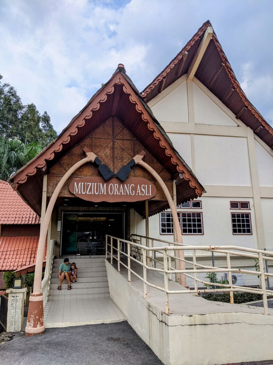

Къща на хора от племето мах мери на остров Кери / Музеят на коренните жители на Малайзия в Гомбак / Обичайни украшения на оранг асли – нанизи от семена или бобчета от джунглата
Друг интересен подход е, че насочват страха на децата си към сферата на нечовешкото. Страшни са гръмотевиците, страшни са тигрите. Хората не бива и не могат да бъдат страшни един за друг – те са, за да се подкрепят, когато ги сполети истински страшното.
Средният глас е сред любимите ми техни стратегии. Темиарите смятат, че насилието се просмуква първо в думите, затова обръщат сериозно внимание на това как говорят.
От малки учат децата си да открият своя среден глас – ще рече, да съчетаят своя глас с този на другия, бил той животно или човек.
Първо това упражнение минава през имитация и пресъздаване на гласовете на различни животни, съвсем буквално сдружаване на два гласа. После идеята е децата все по-тренирано да могат да си представят какво казват те, но и какво би казал другият. Така в състояние на конфликт имат вътрешната настройка да чуват не само своя собствен глас.
Lemme be
Аз съм малаец,
казва Вин Сен Куу. „А вкъщи на какъв език си говорите?“, питам. „На хокиен*“, отвръща той.
Момчето говори китайски, малайски и английски – три езика, като много от хората тук. В Малайзия това е устойчив феномен – може да си четвърто, пето поколение преселник, да говориш у дома на индийски или арабски, но щом те попитат какъв си, отговорът е малаец.



Индийци носят стомни с краве мляко за бог Муруган на големия си празник Тайпусам / Ние и Вин Сен Куу, малайският китаец, който държи корейски ресторант / Арабин, който прави кюнефе в по-строго мюсюлманската част на Малайзия
Така беше и с Арека – пето поколение тамилка, която у дома говори на тамилски, готви предимно тамилски ястия и празнува Дивали (индийски празник на светлината), но същевременно се определя като малайка. Подобна е и житейската нишка на Шели Шахадан – баба ѝ е от Тайланд, дядо ѝ – афганистанец, но тя самата е родена в Куала Лумпур и е малайка.
Най-характерното за нас тук е lemme be,
смее се Шели и говори на брилянтен английски. „Какво е това?“, кокоря се аз. Шели обяснява, че е съкратено от Let me be me – „Остави ме да си бъда аз“.
* Хокиен – група китайски езици.
Всички снимки в статията са собственост на авторката.
Celebrating the community: Micah
Post Syndicated from Sophie Ashford original https://www.raspberrypi.org/blog/celebrating-the-community-micah/
We love hearing from members of the community and sharing the stories of inspiring young people, volunteers, and educators all over the world who have a passion for technology.

With this latest story, we’re taking you to Leeds, UK, to meet Micah, a young space enthusiast whose confidence has soared since he started attending a Code Club at his local library.
Introducing Micah
Computing skills are essential in today’s world, and Micah’s mum Catherine was keen for him to be introduced to coding from a young age.
While Micah is known to people close to him for his inquisitive nature, cheeky behaviour, and quick-witted sense of humour, he can be a little shy when meeting new people. And he isn’t always keen on his mum’s suggestions about trying new things and attending after-school clubs! However, when Catherine saw there was a Code Club running at their local library, she knew it was the perfect opportunity for Micah to try out computing.

What Catherine didn’t know is that not only would Micah find out he was a talented coder, but Code Club would also set the path for him to become a regular attendee at many of the library’s other clubs.
Opportunities for young coders
Based in Leeds, the Compton Centre Code Club is part of the Leeds Libraries network, which runs seven Code Clubs throughout the city. Liam, Senior Librarian for Digital at Leeds Libraries, described the importance of these spaces for the community and for engaging children in tech:
“Libraries are safe spaces that provide free access to exciting and innovative technology to those in our communities who might not get that opportunity. We’re proud that our Code Clubs can support young people to engage with tech, learn some new skills, and meet like-minded peers in a friendly and positive environment.
Our Code Clubs are aimed at 9- to 13-year-olds. We do have some learners that will come that have a younger sister or brother that wants to get involved as well. We never want to turn anyone away. So we’re more than welcoming for that age group to come in and have a play, get used to the equipment, and join in.”
— Liam, Senior Librarian for Digital at Leeds Libraries
Coding and confidence
Code Club provides a safe and friendly space for Micah to connect with other children, and he has embraced coding with enthusiasm. This is possible thanks to the work, support, and encouragement of Micah’s Code Club mentor Basia (they/them), the librarian at the Compton Centre who runs the club.
“Micah loves coming [to Code Club] and learning all the different things that he can do with coding. And he also loves Basia. They’re brilliant and run the club really well. It’s a super child-friendly place to be and he loves the support that he gets from them.”
– Catherine, Micah’s mum
Support from an inspiring mentor is so often an important part of a young coder’s journey, and Basia’s own journey from a coding beginner to a confident mentor highlights the positive influence Code Club has on both children and mentors.

Basia reflected on how they felt when they first heard they were going to be running Code Club sessions, and how their skills and confidence have grown.
“I was daunted for a bit. But actually one of the first things I did when I started this job was to go through some of [the Raspberry Pi Foundation’s] resources and do a project in Scratch. And it was just so simple and straightforward. You know, all the resources are absolutely great and I don’t really need to think about it. I think my confidence has increased quite significantly.”
— Basia, Librarian and Code Club mentor
Since joining Code Club, Micah has become involved in other extracurricular activities, like Lego club and drama club. These experiences have contributed to Micah’s overall personal growth, showcasing the transformative power of Code Club for children.

Micah has exciting dreams for the future, including becoming an astrophysicist, a marine biologist, and the founder of a company named Save The Planet. Supported by dedicated mentors like Basia, Code Clubs are not just about teaching coding — they are helping shape the leaders of tomorrow.
Inspire young people in your community
If you are interested in encouraging your child to explore coding, take a look at the free coding project resources we have available to support you. If you would like to set up a Code Club for young people in your community, head to codeclub.org for information and support.
Help us celebrate Micah and his inspiring journey by sharing his story on X (formerly Twitter), LinkedIn, and Facebook.
The post Celebrating the community: Micah appeared first on Raspberry Pi Foundation.
Comic for 2024.03.19 – Chaps
Post Syndicated from Explosm.net original https://explosm.net/comics/chaps
New Cyanide and Happiness Comic
Man Yue Mo: Gaining kernel code execution on an MTE-enabled Pixel 8
Post Syndicated from corbet original https://lwn.net/Articles/965926/
Man Yue Mo explains
how to compromise a Pixel 8 phone even when the Arm memory-tagging extension is in use, by taking
advantage of the Mali GPU.
So, by using the GPU to access physical addresses directly, I’m
able to completely bypass the protection that MTE
offers. Ultimately, there is no memory safe code in the code that
manages memory accesses. At some point, physical addresses will
have to be used directly to access memory.
Redefining fleet management at Cloudflare
Post Syndicated from Ryan De Lap original https://blog.cloudflare.com/redefining-fleet-management-at-cloudflare

As Cloudflare continues to grow, we are constantly provisioning new servers, data centers, and hardware all over the globe. With this increase in scale it became necessary to re-evaluate our approach to node and datacenter tooling. In this blog post, we explore an in-house infrastructure system we’ve built, called Zinc, to step up to the task. This system, built in Rust, has become an essential part of system engineering, platform management, and provisioning at Cloudflare, while providing user-friendly engineering tools and automations for Cloudflare employees to leverage.
The nature of Zinc is a rather simple system, providing first class data models for logical and physical infrastructure assets here at Cloudflare. Items such as servers (nodes), network devices, and data centers are all members of Zinc, modeled in a strongly-typed system. With these models, Zinc enables powerful APIs, integrations, and interfaces for efficient fleet management on top of this data. Tasks such as assigning workloads to nodes, scheduling any type of data center maintenance, querying data about our fleet, or even managing the repair cycle of faulty nodes are greatly simplified through Zinc and its integrations with other Cloudflare systems.
By providing Cloudflare engineers with a native web interface and command line tooling for interacting with Zinc’s data, a central pane of a glass has been created, where the ability to expand, build, and monitor our fleet has never been easier.
Humble Beginnings
Several years ago, workload management and server provisioning was a tedious process. For our control plane data centers, we would define the workload for every node in massive source-controlled YAML files, sometimes as long as 80,000 lines. Each entry was a node, its name, its rack, and roles to be read by our configuration management software for assignment.
compute5545:
    rack: 219
    clickhouse:
      cluster: dns
    comment: |-
      Updated by <user>
As time went on, this became extremely cumbersome for engineers to manage and assign workloads for servers. Engineers would often have to update multiple files, updating every entry to assign and change workload data by hand. While this may seem like a slight inconvenience at first, when provisioning new hardware or changing workload configuration data, engineers would have to update hundreds of lines of YAML. Additionally, this data was not readily accessible to other systems and automation to read and modify. It became clear that this pattern could not scale, and a stronger framework would need to be created to manage this information.
First, we aimed to tackle this problem by making nodes and their workloads — which we call roles — first class data structures. Workload and node information were collected and stored in this new system called Zinc, and our configuration management system Salt began to read this information not from the YAML files, but a new RESTful API. We also added several features to Zinc to administer and manage node data:
- Workload Management – Zinc assumed the role of the source of truth for node workloads, also taking charge of metadata management for roles. Attributes like a node’s associated cluster or its designated kernel version are now managed through Zinc, eliminating the need for lengthy configuration files scattered across our repositories.
- Least-Privilege User Accounts – Leveraging Cloudflare Access, every Cloudflare employee who uses Zinc has an individual account, with scoped permissions for their job role. This prevents potentially compromised or prying users from viewing sensitive asset information, and makes modifications to production systems impossible without approval.
- Change Request and Approval System – Zinc implements a change request system, similar to pull requests, so nodes and their associated workloads require approval from the team that manages the workload. For example, if a Cloudflare engineer wanted to provision and assign new Kubernetes nodes, this action would require approval by the Kubernetes team before being applied.
- Node Reservations – It can become necessary for Cloudflare engineers to reserve specific hardware for testing and future workload capacity. Zinc provides this functionality as a first-class operation, providing a clear view into what a node is being used for, even when not in production. A common pattern to see is spare hardware for roles like Postgres or Clickhouse reserved and ready to take over if other nodes need to be taken out of production.
- Node Metadata – Zinc collects a variety of node asset data through other subsystems at Cloudflare, unifying it all under a single pane of glass. Hardware information such as CPU, memory, generation, chassis, power, and networking configuration are all members of Zinc’s APIs and interfaces.
These were the initial features Zinc offered to Cloudflare’s SRE teams, but over time needs grew to expand the scope and start handling a variety of asset and operational data. Zinc has since started representing and managing more infrastructure related to network devices and datacenter management.
System Blueprint
At Cloudflare, two critical systems, Zinc and Netbox, play complementary roles in managing infrastructure. Zinc specializes in handling the logical infrastructure and operational configuration, while Netbox focuses on physical infrastructure. For those unfamiliar with Netbox, it plays the important role of acting as our Datacenter Inventory Management System (DCIM). Details such as hardware specifications, serial numbers, cable diagrams, and rack layouts are all stored in Netbox. These elements are the building blocks of the infrastructure that Zinc imports and relies on to create higher level abstractions, useful for a variety of systems on Cloudflare to depend on, without having to know the nitty-gritty specifics of our datacenter information.
Supercharged Automations
Growing pains were inevitable given the sheer pace of Cloudflare’s growth. Processes around server provisioning, maintenance windows, repairs, and diagnostics reporting were reaching their limits. Luckily, the data available through Zinc made it a natural home for new and improved workflow automations aimed at removing toil across various touch points throughout a server’s lifecycle.
Repairs
Hardware failures are common at our scale. Issues such as disk failure, motherboard problems, or CPU voltage errors are just a few of the many common failures seen in production. While Cloudflare’s infrastructure is very fault tolerant, we want to quickly return hardware to production after a failure to increase capacity and optimize infrastructure costs. Prior to Zinc, engineers would have to manually collect and file tickets with information related to the hardware failure, tediously filling ticket details manually in order for data center technicians to service it. With Zinc, however, the process of collecting this data and generating repair tickets is entirely automated. As we continue developing Zinc, we will be able to manage this process all the way down to the individual hardware component level and enhance existing automation and diagnostic integrations, further optimizing the repair process. With just a few clicks (or driven by other automation), an accurate service ticket can be filed, enabling data center technicians to make repairs and get servers back into production as fast as possible.
Diagnostic Reports
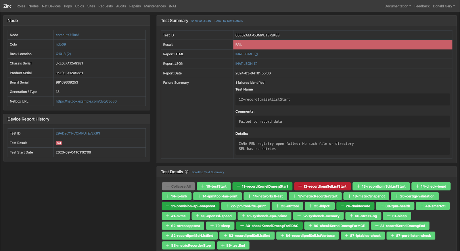
Zinc integrates directly with a diagnostic service we use to identify hardware issues on our fleet, known as INAT (Integrated Node Acceptance Tests). Zinc leverages this system to run acceptance tests before, during, and after server provisioning. It also can be executed in an ad hoc manner to determine the health of a machine. With INAT, we are able to save engineers time and quickly get results back to aid in the debugging process. Once these diagnostics are complete, the Zinc interface provides a report that can be used to determine the health of a server and if any actions need to be taken.
Maintenance Windows
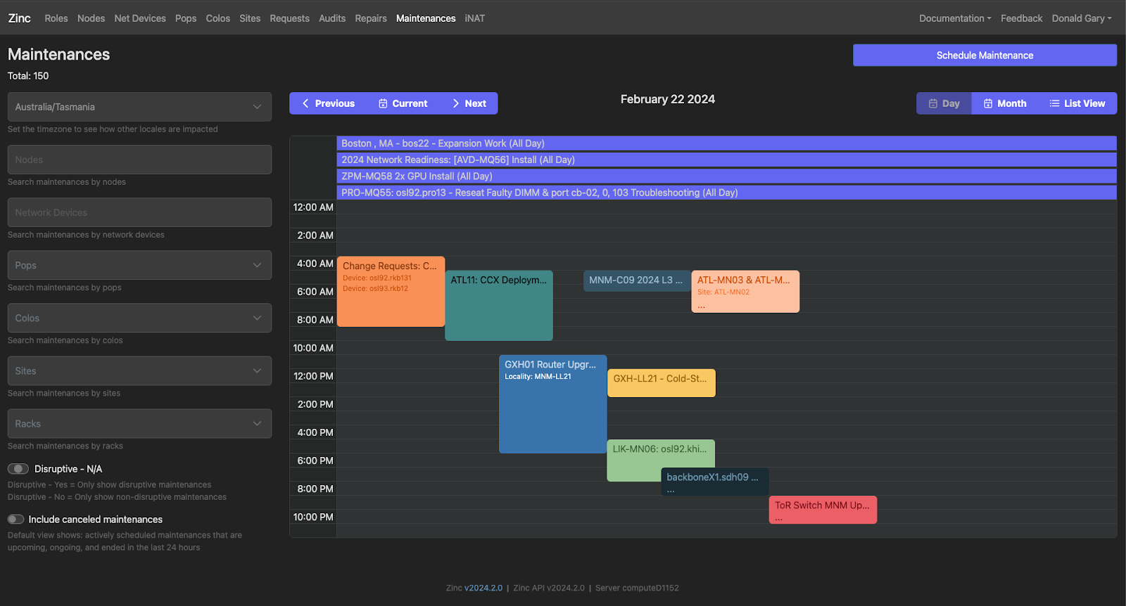
If you’ve ever wondered how the maintenance page on Cloudflare Status is populated, Zinc is the place of origin. As we are constantly doing hardware and network upgrades, it’s important for Cloudflare to have a centralized view of what maintenance is happening, where it is happening, and the scale of all the systems and services that are or can be impacted by the maintenance. During maintenance, there are a variety of automated systems that ensure that Cloudflare sees no loss in quality of service, no matter where in the world the maintenance is happening. Zinc orchestrates and tracks these maintenance windows, and sends alerts to teams and Cloudflare customers when a disruptive, or even potentially disruptive, maintenance is scheduled in a region.
Reboots
Zinc provides an integration with a core system responsible for scheduling node reboots. When a node needs to be rebooted, such as to apply a new firmware upgrade or new Kernel version, there are systems at Cloudflare that schedule and safely manage this functionality. For example, it would be unsafe to reboot a production Clickhouse node with no prior warning, so these systems ensure traffic is properly routed away from this node prior to its reboot. Zinc provides an integration in its Web UI and CLI with this reboot management system to make the process of queuing and executing reboots much easier, as well as providing a place where we can add orchestration logic that leverages Zinc’s operational management capabilities for server reboots.
Engineer Productivity
One of the most valuable parts of Zinc is that it provides engineers the ability to quickly perform complex queries and apply changes to our assets in production. At the API layer, we ensure that any access or changes to our infrastructure are properly scoped and authenticated. From there, Zinc provides two interfaces for employees managing our fleet: a command-line interface built in Rust, and a web application built in React, both of which are built on the same Zinc API that can be directly called from scripts or other systems as integrations are built out to automate more of the management of our infrastructure.
Here are some common examples of the CLI tooling our engineers use:
# List all datacenters at Cloudflare
$ zinc site get --all
# Set a node's status to disabled, removing it from production.
$ zinc node update status compute5545 disabled
# Querying all nodes in a specific rack, that are Kubernetes nodes.
$ zinc node get -f "rack:A413" -f “role:kubernetes”
# Putting a node failure into a repair state with debug information on how to fix.
$ zinc repair node create –name 36com360 --repair-type motherboard –remove-from-prod –comments “Diagnostic determined bad motherboard”
While these are simple queries, Zinc also provides its own query syntax to get more detailed information using its own query structure. Here we see an example of looking for Kubernetes workers that are a part of our pdx cluster, while ignoring storage and rook nodes.
zinc node get -f 'role:kubernetes.cluster=pdx&kubernetes.worker=true&!kubernetes.storage&!kubernetes.rook'
Node Name    Node Type  Node Status  Colo ID  Colo Name  Rack  Rack Unit  Roles
compute2712  compute     V           348      pdx05      B103  39         kubernetes
compute1995  compute     V           349      pdx06      A104  7          kubernetes
compute1192  compute     V           36       pdx01      A203  10         kubernetes
…
Total records: 1337
Web UI
Despite being an internal tool, we felt it necessary to ensure that the UX of Zinc was intuitive and crisp. As it stands, hundreds of engineers at Cloudflare rely on Zinc’s web interface, so we found it essential to provide a fast, easy to use design. Built in React as a single page application, we aim to optimize for ease of use wherever possible. Querying items such as assets in repair, nodes in a specific city or country, or even CPU model are all first-class searchable items in our UI.
As mentioned previously, Zinc also provides a user-friendly Change Request interface, similar to Git Pull Requests, which shows what asset data is changing and who is making the change, and ensures the change is approved by designated staff prior to being applied in production.
Looking Ahead
Zinc represents a significant advancement in infrastructure management at Cloudflare. With our fleet growing faster than ever, especially with our new expansions to deliver GPUs on the Edge and Cloudflare’s R2, Zinc has stepped up to the plate, tackling the challenges of growth and providing invaluable support to our engineering teams. We hope this has been an insightful view of how Cloudflare is building to grow and scale well into the future.
There are still many wins to be had when it comes to infrastructure tooling here at Cloudflare. In the long term, Zinc will continue to be the backbone of infrastructure and asset data, with deeper automations and integrations to save our engineers time and toil and reduce manual errors as we continue to expand.
If managing and operating a fleet of servers as large as Cloudflare sounds like an exciting challenge to you, we’re hiring!
Canon 200-800mm – Great Value ULTRA Telephoto Zoom
Post Syndicated from Matt Granger original https://www.youtube.com/watch?v=B50euvi2BH0
AI and the Evolution of Social Media
Post Syndicated from Bruce Schneier original https://www.schneier.com/blog/archives/2024/03/ai-and-the-evolution-of-social-media.html
Oh, how the mighty have fallen. A decade ago, social media was celebrated for sparking democratic uprisings in the Arab world and beyond. Now front pages are splashed with stories of social platforms’ role in misinformation, business conspiracy, malfeasance, and risks to mental health. In a 2022 survey, Americans blamed social media for the coarsening of our political discourse, the spread of misinformation, and the increase in partisan polarization.
Today, tech’s darling is artificial intelligence. Like social media, it has the potential to change the world in many ways, some favorable to democracy. But at the same time, it has the potential to do incredible damage to society.
There is a lot we can learn about social media’s unregulated evolution over the past decade that directly applies to AI companies and technologies. These lessons can help us avoid making the same mistakes with AI that we did with social media.
In particular, five fundamental attributes of social media have harmed society. AI also has those attributes. Note that they are not intrinsically evil. They are all double-edged swords, with the potential to do either good or ill. The danger comes from who wields the sword, and in what direction it is swung. This has been true for social media, and it will similarly hold true for AI. In both cases, the solution lies in limits on the technology’s use.
#1: Advertising
The role advertising plays in the internet arose more by accident than anything else. When commercialization first came to the internet, there was no easy way for users to make micropayments to do things like viewing a web page. Moreover, users were accustomed to free access and wouldn’t accept subscription models for services. Advertising was the obvious business model, if never the best one. And it’s the model that social media also relies on, which leads it to prioritize engagement over anything else.
Both Google and Facebook believe that AI will help them keep their stranglehold on an 11-figure online ad market (yep, 11 figures), and the tech giants that are traditionally less dependent on advertising, like Microsoft and Amazon, believe that AI will help them seize a bigger piece of that market.
Big Tech needs something to persuade advertisers to keep spending on their platforms. Despite bombastic claims about the effectiveness of targeted marketing, researchers have long struggled to demonstrate where and when online ads really have an impact. When major brands like Uber and Procter & Gamble recently slashed their digital ad spending by the hundreds of millions, they proclaimed that it made no dent at all in their sales.
AI-powered ads, industry leaders say, will be much better. Google assures you that AI can tweak your ad copy in response to what users search for, and that its AI algorithms will configure your campaigns to maximize success. Amazon wants you to use its image generation AI to make your toaster product pages look cooler. And IBM is confident its Watson AI will make your ads better.
These techniques border on the manipulative, but the biggest risk to users comes from advertising within AI chatbots. Just as Google and Meta embed ads in your search results and feeds, AI companies will be pressured to embed ads in conversations. And because those conversations will be relational and human-like, they could be more damaging. While many of us have gotten pretty good at scrolling past the ads in Amazon and Google results pages, it will be much harder to determine whether an AI chatbot is mentioning a product because it’s a good answer to your question or because the AI developer got a kickback from the manufacturer.
#2: Surveillance
Social media’s reliance on advertising as the primary way to monetize websites led to personalization, which led to ever-increasing surveillance. To convince advertisers that social platforms can tweak ads to be maximally appealing to individual people, the platforms must demonstrate that they can collect as much information about those people as possible.
It’s hard to exaggerate how much spying is going on. A recent analysis by Consumer Reports about Facebook—just Facebook—showed that every user has more than 2,200 different companies spying on their web activities on its behalf.
AI-powered platforms that are supported by advertisers will face all the same perverse and powerful market incentives that social platforms do. It’s easy to imagine that a chatbot operator could charge a premium if it were able to claim that its chatbot could target users on the basis of their location, preference data, or past chat history and persuade them to buy products.
The possibility of manipulation is only going to get greater as we rely on AI for personal services. One of the promises of generative AI is the prospect of creating a personal digital assistant advanced enough to act as your advocate with others and as a butler to you. This requires more intimacy than you have with your search engine, email provider, cloud storage system, or phone. You’re going to want it with you constantly, and to most effectively work on your behalf, it will need to know everything about you. It will act as a friend, and you are likely to treat it as such, mistakenly trusting its discretion.
Even if you choose not to willingly acquaint an AI assistant with your lifestyle and preferences, AI technology may make it easier for companies to learn about you. Early demonstrations illustrate how chatbots can be used to surreptitiously extract personal data by asking you mundane questions. And with chatbots increasingly being integrated with everything from customer service systems to basic search interfaces on websites, exposure to this kind of inferential data harvesting may become unavoidable.
#3: Virality
Social media allows any user to express any idea with the potential for instantaneous global reach. A great public speaker standing on a soapbox can spread ideas to maybe a few hundred people on a good night. A kid with the right amount of snark on Facebook can reach a few hundred million people within a few minutes.
A decade ago, technologists hoped this sort of virality would bring people together and guarantee access to suppressed truths. But as a structural matter, it is in a social network’s interest to show you the things you are most likely to click on and share, and the things that will keep you on the platform.
As it happens, this often means outrageous, lurid, and triggering content. Researchers have found that content expressing maximal animosity toward political opponents gets the most engagement on Facebook and Twitter. And this incentive for outrage drives and rewards misinformation.
As Jonathan Swift once wrote, “Falsehood flies, and the Truth comes limping after it.” Academics seem to have proved this in the case of social media; people are more likely to share false information—perhaps because it seems more novel and surprising. And unfortunately, this kind of viral misinformation has been pervasive.
AI has the potential to supercharge the problem because it makes content production and propagation easier, faster, and more automatic. Generative AI tools can fabricate unending numbers of falsehoods about any individual or theme, some of which go viral. And those lies could be propelled by social accounts controlled by AI bots, which can share and launder the original misinformation at any scale.
Remarkably powerful AI text generators and autonomous agents are already starting to make their presence felt in social media. In July, researchers at Indiana University revealed a botnet of more than 1,100 Twitter accounts that appeared to be operated using ChatGPT.
AI will help reinforce viral content that emerges from social media. It will be able to create websites and web content, user reviews, and smartphone apps. It will be able to simulate thousands, or even millions, of fake personas to give the mistaken impression that an idea, or a political position, or use of a product, is more common than it really is. What we might perceive to be vibrant political debate could be bots talking to bots. And these capabilities won’t be available just to those with money and power; the AI tools necessary for all of this will be easily available to us all.
#4: Lock-in
Social media companies spend a lot of effort making it hard for you to leave their platforms. It’s not just that you’ll miss out on conversations with your friends. They make it hard for you to take your saved data—connections, posts, photos—and port it to another platform. Every moment you invest in sharing a memory, reaching out to an acquaintance, or curating your follows on a social platform adds a brick to the wall you’d have to climb over to go to another platform.
This concept of lock-in isn’t unique to social media. Microsoft cultivated proprietary document formats for years to keep you using its flagship Office product. Your music service or e-book reader makes it hard for you to take the content you purchased to a rival service or reader. And if you switch from an iPhone to an Android device, your friends might mock you for sending text messages in green bubbles. But social media takes this to a new level. No matter how bad it is, it’s very hard to leave Facebook if all your friends are there. Coordinating everyone to leave for a new platform is impossibly hard, so no one does.
Similarly, companies creating AI-powered personal digital assistants will make it hard for users to transfer that personalization to another AI. If AI personal assistants succeed in becoming massively useful time-savers, it will be because they know the ins and outs of your life as well as a good human assistant; would you want to give that up to make a fresh start on another company’s service? In extreme examples, some people have formed close, perhaps even familial, bonds with AI chatbots. If you think of your AI as a friend or therapist, that can be a powerful form of lock-in.
Lock-in is an important concern because it results in products and services that are less responsive to customer demand. The harder it is for you to switch to a competitor, the more poorly a company can treat you. Absent any way to force interoperability, AI companies have less incentive to innovate in features or compete on price, and fewer qualms about engaging in surveillance or other bad behaviors.
#5: Monopolization
Social platforms often start off as great products, truly useful and revelatory for their consumers, before they eventually start monetizing and exploiting those users for the benefit of their business customers. Then the platforms claw back the value for themselves, turning their products into truly miserable experiences for everyone. This is a cycle that Cory Doctorow has powerfully written about and traced through the history of Facebook, Twitter, and more recently TikTok.
The reason for these outcomes is structural. The network effects of tech platforms push a few firms to become dominant, and lock-in ensures their continued dominance. The incentives in the tech sector are so spectacularly, blindingly powerful that they have enabled six megacorporations (Amazon, Apple, Google, Facebook parent Meta, Microsoft, and Nvidia) to command a trillion dollars each of market value—or more. These firms use their wealth to block any meaningful legislation that would curtail their power. And they sometimes collude with each other to grow yet fatter.
This cycle is clearly starting to repeat itself in AI. Look no further than the industry poster child OpenAI, whose leading offering, ChatGPT, continues to set marks for uptake and usage. Within a year of the product’s launch, OpenAI’s valuation had skyrocketed to about $90 billion.
OpenAI once seemed like an “open” alternative to the megacorps—a common carrier for AI services with a socially oriented nonprofit mission. But the Sam Altman firing-and-rehiring debacle at the end of 2023, and Microsoft’s central role in restoring Altman to the CEO seat, simply illustrated how venture funding from the familiar ranks of the tech elite pervades and controls corporate AI. In January 2024, OpenAI took a big step toward monetization of this user base by introducing its GPT Store, wherein one OpenAI customer can charge another for the use of its custom versions of OpenAI software; OpenAI, of course, collects revenue from both parties. This sets in motion the very cycle Doctorow warns about.
In the middle of this spiral of exploitation, little or no regard is paid to externalities visited upon the greater public—people who aren’t even using the platforms. Even after society has wrestled with their ill effects for years, the monopolistic social networks have virtually no incentive to control their products’ environmental impact, tendency to spread misinformation, or pernicious effects on mental health. And the government has applied virtually no regulation toward those ends.
Likewise, few or no guardrails are in place to limit the potential negative impact of AI. Facial recognition software that amounts to racial profiling, simulated public opinions supercharged by chatbots, fake videos in political ads—all of it persists in a legal gray area. Even clear violators of campaign advertising law might, some think, be let off the hook if they simply do it with AI.
Mitigating the risks
The risks that AI poses to society are strikingly familiar, but there is one big difference: it’s not too late. This time, we know it’s all coming. Fresh off our experience with the harms wrought by social media, we have all the warning we should need to avoid the same mistakes.
The biggest mistake we made with social media was leaving it as an unregulated space. Even now—after all the studies and revelations of social media’s negative effects on kids and mental health, after Cambridge Analytica, after the exposure of Russian intervention in our politics, after everything else—social media in the US remains largely an unregulated “weapon of mass destruction.” Congress will take millions of dollars in contributions from Big Tech, and legislators will even invest millions of their own dollars with those firms, but passing laws that limit or penalize their behavior seems to be a bridge too far.
We can’t afford to do the same thing with AI, because the stakes are even higher. The harm social media can do stems from how it affects our communication. AI will affect us in the same ways and many more besides. If Big Tech’s trajectory is any signal, AI tools will increasingly be involved in how we learn and how we express our thoughts. But these tools will also influence how we schedule our daily activities, how we design products, how we write laws, and even how we diagnose diseases. The expansive role of these technologies in our daily lives gives for-profit corporations opportunities to exert control over more aspects of society, and that exposes us to the risks arising from their incentives and decisions.
The good news is that we have a whole category of tools to modulate the risk that corporate actions pose for our lives, starting with regulation. Regulations can come in the form of restrictions on activity, such as limitations on what kinds of businesses and products are allowed to incorporate AI tools. They can come in the form of transparency rules, requiring disclosure of what data sets are used to train AI models or what new preproduction-phase models are being trained. And they can come in the form of oversight and accountability requirements, allowing for civil penalties in cases where companies disregard the rules.
The single biggest point of leverage governments have when it comes to tech companies is antitrust law. Despite what many lobbyists want you to think, one of the primary roles of regulation is to preserve competition—not to make life harder for businesses. It is not inevitable for OpenAI to become another Meta, an 800-pound gorilla whose user base and reach are several times those of its competitors. In addition to strengthening and enforcing antitrust law, we can introduce regulation that supports competition-enabling standards specific to the technology sector, such as data portability and device interoperability. This is another core strategy for resisting monopoly and corporate control.
Additionally, governments can enforce existing regulations on advertising. Just as the US regulates what media can and cannot host advertisements for sensitive products like cigarettes, and just as many other jurisdictions exercise strict control over the time and manner of politically sensitive advertising, so too could the US limit the engagement between AI providers and advertisers.
Lastly, we should recognize that developing and providing AI tools does not have to be the sovereign domain of corporations. We, the people and our government, can do this too. The proliferation of open-source AI development in 2023, successful to an extent that startled corporate players, is proof of this. And we can go further, calling on our government to build public-option AI tools developed with political oversight and accountability under our democratic system, where the dictatorship of the profit motive does not apply.
Which of these solutions is most practical, most important, or most urgently needed is up for debate. We should have a vibrant societal dialogue about whether and how to use each of these tools. There are lots of paths to a good outcome.
The problem is that this isn’t happening now, particularly in the US. And with a looming presidential election, conflict spreading alarmingly across Asia and Europe, and a global climate crisis, it’s easy to imagine that we won’t get our arms around AI any faster than we have (not) with social media. But it’s not too late. These are still the early years for practical consumer AI applications. We must and can do better.
This essay was written with Nathan Sanders, and was originally published in MIT Technology Review.
insecurity system
Post Syndicated from turnoff.us original http://turnoff.us/geek/insecurity-system/

New Intermediate Certificates
Post Syndicated from Let's Encrypt original https://letsencrypt.org/2024/03/19/new-intermediate-certificates/
On Wednesday, March 13, 2024, Let’s Encrypt generated 10 new Intermediate CA Key Pairs, and issued 15 new Intermediate CA Certificates containing the new public keys. These new intermediate certificates provide smaller and more efficient certificate chains to Let’s Encrypt Subscribers, enhancing the overall online experience in terms of speed, security, and accessibility.
First, a bit of history. In September, 2020, Let’s Encrypt issued a new root and collection of intermediate certificates. Those certificates helped us improve the privacy and efficiency of Web security by making ECDSA end-entity certificates widely available. However, those intermediates are approaching their expiration dates, so it is time to replace them.
Our new batch of intermediates are very similar to the ones we issued in 2020, with a few small changes. We’re going to go over what those changes are and why we made them.
The New Certificates
We created 5 new 2048-bit RSA intermediate certificates named in sequence from R10 through R14. These are issued by ISRG Root X1. You can think of them as direct replacements for our existing R3 and R4 intermediates.
We also created 5 new P-384 ECDSA intermediate certificates named in sequence from E5 through E9. Each of these is represented by two certificates: one issued by ISRG Root X2 (exactly like our existing E1 and E2), and one issued (or cross-signed) by ISRG Root X1.
You can see details of all of the certificates on our updated hierarchy page.
Rotating Issuance
Rotating the set of intermediates we issue from helps keep the Internet agile and more secure. It encourages automation and efficiency, and discourages outdated practices like key pinning. “Key Pinning” is a practice in which clients — either ACME clients getting certificates for their site, or apps connecting to their own backend servers — decide to trust only a single issuing intermediate certificate rather than delegating trust to the system trust store. Updating pinned keys is a manual process, which leads to an increased risk of errors and potential business continuity failures.
Intermediates usually change only every five years, so this joint is exercised infrequently and client software keeps making the same mistakes. Shortening the lifetime from five years to three years means we will be conducting another ceremony in just two years, ahead of the expiration date on these recently created certificates. This ensures we exercise the joint more frequently than in the past.
We also issued more intermediates this time around. Historically, we’ve had two of each key type (RSA and ECDSA): one for active issuance, and one held as a backup for emergencies. Moving forward we will have five: two conducting active issuance, two waiting in the wings to be introduced in about one year, and one for emergency backup. Randomizing the selected issuer for a given key type means it will be impossible to predict which intermediate a certificate will be issued from. We are very hopeful that these steps will prevent intermediate key pinning altogether, and help the WebPKI remain agile moving forward.
These shorter intermediate lifetimes and randomized intermediate issuance shouldn’t impact the online experience of the general Internet user. Subscribers may be impacted if they are pinning one of our intermediates, though this should be incredibly rare.
Providing Smaller Chains
When we issued ISRG Root X2 in 2020, we decided to cross-sign it from ISRG Root X1 so that it would be trusted even by systems that didn’t yet have ISRG Root X2 in their trust store. This meant that Subscribers who wanted issuance from our ECDSA intermediates would have a choice: they could either have a very short, ECDSA-only, but low-compatibility chain terminating at ISRG Root X2, or they could have a longer, high-compatibility chain terminating at ISRG Root X1. At the time, this tradeoff (TLS handshake size vs compatibility) seemed like a reasonable choice to provide, and we provided the high-compatibility chain by default to support the largest number of configurations.
ISRG Root X2 is now trusted by most platforms, and we can now offer an improved version of the same choice. The same very short, ECDSA-only chain will still be available for Subscribers who want to optimize their TLS handshakes at the cost of some compatibility. But the high-compatibility chain will be drastically improving: instead of containing two intermediates (both E1 and the cross-signed ISRG Root X2), it will now contain only a single intermediate: the version of one of our new ECDSA intermediates cross-signed by ISRG Root X1.
This reduces the size of our default ECDSA chain by about a third, and is an important step towards removing our ECDSA allow-list.
Other Minor Changes
We’ve made two other tiny changes that are worth mentioning, but will have no impact on how Subscribers and clients use our certificates:
-
We’ve changed how the Subject Key ID field is calculated, from a SHA-1 hash of the public key, to a truncated SHA-256 hash of the same data. Although this use of SHA-1 was not cryptographically relevant, it is still nice to remove one more usage of that broken algorithm, helping move towards a world where cryptography libraries don’t need to include SHA-1 support at all.
-
We have removed our CPS OID from the Certificate Policies extension. This saves a few bytes in the certificate, which can add up to a lot of bandwidth saved over the course of billions of TLS handshakes.
Both of these mirror two identical changes that we made for our Subscriber Certificates in the past year.
Deployment
We intend to put two of each of the new RSA and ECDSA keys into rotation in the next few months. Two of each will be ready to swap in at a future date, and one of each will be held in reserve in case of an emergency. Read more about the strategy in our December 2023 post on the Community Forum.
Not familiar with the forum? It’s where Let’s Encrypt publishes updates on our Issuance Tech and APIs. It’s also where you can go for troubleshooting help from community experts and Let’s Encrypt staff. Check it out and subscribe to alerts for technical updates.
We hope that this has been an interesting and informative tour around our new intermediates, and we look forward to continuing to improve the Internet, one certificate at a time.
We depend on contributions from our community of users and supporters in order to provide our services. If your company or organization would like to sponsor Let’s Encrypt please email us at [email protected]. We ask that you make an individual contribution if it is within your means.
New Intermediate Certificates
Post Syndicated from Let's Encrypt original https://letsencrypt.org/2024/03/19/new-intermediate-certificates.html
On Wednesday, March 13, 2024, Let’s Encrypt generated 10 new Intermediate CA Key Pairs, and issued 15 new Intermediate CA Certificates containing the new public keys. These new intermediate certificates provide smaller and more efficient certificate chains to Let’s Encrypt Subscribers, enhancing the overall online experience in terms of speed, security, and accessibility.
First, a bit of history. In September, 2020, Let’s Encrypt issued a new root and collection of intermediate certificates. Those certificates helped us improve the privacy and efficiency of Web security by making ECDSA end-entity certificates widely available. However, those intermediates are approaching their expiration dates, so it is time to replace them.
Our new batch of intermediates are very similar to the ones we issued in 2020, with a few small changes. We’re going to go over what those changes are and why we made them.
The New Certificates
We created 5 new 2048-bit RSA intermediate certificates named in sequence from R10 through R14. These are issued by ISRG Root X1. You can think of them as direct replacements for our existing R3 and R4 intermediates.
We also created 5 new P-384 ECDSA intermediate certificates named in sequence from E5 through E9. Each of these is represented by two certificates: one issued by ISRG Root X2 (exactly like our existing E1 and E2), and one issued (or cross-signed) by ISRG Root X1.
You can see details of all of the certificates on our updated hierarchy page.
Rotating Issuance
Rotating the set of intermediates we issue from helps keep the Internet agile and more secure. It encourages automation and efficiency, and discourages outdated practices like key pinning. “Key Pinning” is a practice in which clients — either ACME clients getting certificates for their site, or apps connecting to their own backend servers — decide to trust only a single issuing intermediate certificate rather than delegating trust to the system trust store. Updating pinned keys is a manual process, which leads to an increased risk of errors and potential business continuity failures.
Intermediates usually change only every five years, so this joint is exercised infrequently and client software keeps making the same mistakes. Shortening the lifetime from five years to three years means we will be conducting another ceremony in just two years, ahead of the expiration date on these recently created certificates. This ensures we exercise the joint more frequently than in the past.
We also issued more intermediates this time around. Historically, we’ve had two of each key type (RSA and ECDSA): one for active issuance, and one held as a backup for emergencies. Moving forward we will have five: two conducting active issuance, two waiting in the wings to be introduced in about one year, and one for emergency backup. Randomizing the selected issuer for a given key type means it will be impossible to predict which intermediate a certificate will be issued from. We are very hopeful that these steps will prevent intermediate key pinning altogether, and help the WebPKI remain agile moving forward.
These shorter intermediate lifetimes and randomized intermediate issuance shouldn’t impact the online experience of the general Internet user. Subscribers may be impacted if they are pinning one of our intermediates, though this should be incredibly rare.
Providing Smaller Chains
When we issued ISRG Root X2 in 2020, we decided to cross-sign it from ISRG Root X1 so that it would be trusted even by systems that didn’t yet have ISRG Root X2 in their trust store. This meant that Subscribers who wanted issuance from our ECDSA intermediates would have a choice: they could either have a very short, ECDSA-only, but low-compatibility chain terminating at ISRG Root X2, or they could have a longer, high-compatibility chain terminating at ISRG Root X1. At the time, this tradeoff (TLS handshake size vs compatibility) seemed like a reasonable choice to provide, and we provided the high-compatibility chain by default to support the largest number of configurations.
ISRG Root X2 is now trusted by most platforms, and we can now offer an improved version of the same choice. The same very short, ECDSA-only chain will still be available for Subscribers who want to optimize their TLS handshakes at the cost of some compatibility. But the high-compatibility chain will be drastically improving: instead of containing two intermediates (both E1 and the cross-signed ISRG Root X2), it will now contain only a single intermediate: the version of one of our new ECDSA intermediates cross-signed by ISRG Root X1.
This reduces the size of our default ECDSA chain by about a third, and is an important step towards removing our ECDSA allow-list.
Other Minor Changes
We’ve made two other tiny changes that are worth mentioning, but will have no impact on how Subscribers and clients use our certificates:
-
We’ve changed how the Subject Key ID field is calculated, from a SHA-1 hash of the public key, to a truncated SHA-256 hash of the same data. Although this use of SHA-1 was not cryptographically relevant, it is still nice to remove one more usage of that broken algorithm, helping move towards a world where cryptography libraries don’t need to include SHA-1 support at all.
-
We have removed our CPS OID from the Certificate Policies extension. This saves a few bytes in the certificate, which can add up to a lot of bandwidth saved over the course of billions of TLS handshakes.
Both of these mirror two identical changes that we made for our Subscriber Certificates in the past year.
Deployment
We intend to put two of each of the new RSA and ECDSA keys into rotation in the next few months. Two of each will be ready to swap in at a future date, and one of each will be held in reserve in case of an emergency. Read more about the strategy in our December 2023 post on the Community Forum.
Not familiar with the forum? It’s where Let’s Encrypt publishes updates on our Issuance Tech and APIs. It’s also where you can go for troubleshooting help from community experts and Let’s Encrypt staff. Check it out and subscribe to alerts for technical updates.
We hope that this has been an interesting and informative tour around our new intermediates, and we look forward to continuing to improve the Internet, one certificate at a time.
We depend on contributions from our community of users and supporters in order to provide our services. If your company or organization would like to sponsor Let’s Encrypt please email us at [email protected]. We ask that you make an individual contribution if it is within your means.
Amazon Managed Service for Apache Flink now supports Apache Flink version 1.18
Post Syndicated from Lorenzo Nicora original https://aws.amazon.com/blogs/big-data/amazon-managed-service-for-apache-flink-now-supports-apache-flink-version-1-18/
Apache Flink is an open source distributed processing engine, offering powerful programming interfaces for both stream and batch processing, with first-class support for stateful processing and event time semantics. Apache Flink supports multiple programming languages, Java, Python, Scala, SQL, and multiple APIs with different level of abstraction, which can be used interchangeably in the same application.
Amazon Managed Service for Apache Flink, which offers a fully managed, serverless experience in running Apache Flink applications, now supports Apache Flink 1.18.1, the latest version of Apache Flink at the time of writing.
In this post, we discuss some of the interesting new features and capabilities of Apache Flink, introduced with the most recent major releases, 1.16, 1.17, and 1.18, and now supported in Managed Service for Apache Flink.
New connectors
Before we dive into the new functionalities of Apache Flink available with version 1.18.1, let’s explore the new capabilities that come from the availability of many new open source connectors.
OpenSearch
A dedicated OpenSearch connector is now available to be included in your projects, enabling an Apache Flink application to write data directly into OpenSearch, without relying on Elasticsearch compatibility mode. This connector is compatible with Amazon OpenSearch Service provisioned and OpenSearch Service Serverless.
This new connector supports SQL and Table APIs, working with both Java and Python, and the DataStream API, for Java only. Out of the box, it provides at-least-once guarantees, synchronizing the writes with Flink checkpointing. You can achieve exactly-once semantics using deterministic IDs and upsert method.
By default, the connector uses OpenSearch version 1.x client libraries. You can switch to version 2.x by adding the correct dependencies.
Amazon DynamoDB
Apache Flink developers can now use a dedicated connector to write data into Amazon DynamoDB. This connector is based on the Apache Flink AsyncSink, developed by AWS and now an integral part of the Apache Flink project, to simplify the implementation of efficient sink connectors, using non-blocking write requests and adaptive batching.
This connector also supports both SQL and Table APIs, Java and Python, and DataStream API, for Java only. By default, the sink writes in batches to optimize throughput. A notable feature of the SQL version is support for the PARTITIONED BY clause. By specifying one or more keys, you can achieve some client-side deduplication, only sending the latest record per key with each batch write. An equivalent can be achieved with the DataStream API by specifying a list of partition keys for overwriting within each batch.
This connector only works as a sink. You cannot use it for reading from DynamoDB. To look up data in DynamoDB, you still need to implement a lookup using the Flink Async I/O API or implementing a custom user-defined function (UDF), for SQL.
MongoDB
Another interesting connector is for MongoDB. In this case, both source and sink are available, for both the SQL and Table APIs and DataStream API. The new connector is now officially part of the Apache Flink project and supported by the community. This new connector replaces the old one provided by MongoDB directly, which only supports older Flink Sink and Source APIs.
As for other data store connectors, the source can either be used as a bounded source, in batch mode, or for lookups. The sink works both in batch mode and streaming, supporting both upsert and append mode.
Among the many notable features of this connector, one that’s worth mentioning is the ability to enable caching when using the source for lookups. Out of the box, the sink supports at-least-once guarantees. When a primary key is defined, the sink can support exactly-once semantics via idempotent upserts. The sink connector also supports exactly-once semantics, with idempotent upserts, when the primary key is defined.
New connector versioning
Not a new feature, but an important factor to consider when updating an older Apache Flink application, is the new connector versioning. Starting from Apache Flink version 1.17, most connectors have been externalized from the main Apache Flink distribution and follow independent versioning.
To include the right dependency, you need to specify the artifact version with the form: <connector-version>-<flink-version>
For example, the latest Kafka connector, also working with Amazon Managed Streaming for Apache Kafka (Amazon MSK), at the time of writing is version 3.1.0. If you are using Apache Flink 1.18, the dependency to use will be the following:
For Amazon Kinesis, the new connector version is 4.2.0. The dependency for Apache Flink 1.18 will be the following:
In the following sections, we discuss more of the powerful new features now available in Apache Flink 1.18 and supported in Amazon Managed Service for Apache Flink.
SQL
In Apache Flink SQL, users can provide hints to join queries that can be used to suggest the optimizer to have an effect in the query plan. In particular, in streaming applications, lookup joins are used to enrich a table, representing streaming data, with data that is queried from an external system, typically a database. Since version 1.16, several improvements have been introduced for lookup joins, allowing you to adjust the behavior of the join and improve performance:
- Lookup cache is a powerful feature, allowing you to cache in-memory the most frequently used records, reducing the pressure on the database. Previously, lookup cache was specific to some connectors. Since Apache Flink 1.16, this option has become available to all connectors internally supporting lookup (FLIP-221). As of this writing, JDBC, Hive, and HBase connectors support lookup cache. Lookup cache has three available modes:
FULL, for a small dataset that can be held entirely in memory,PARTIAL, for a large dataset, only caching the most recent records, orNONE, to completely disable cache. ForPARTIALcache, you can also configure the number of rows to buffer and the time-to-live. - Async lookup is another feature that can greatly improve performance. Async lookup provides in Apache Flink SQL a functionality similar to Async I/O available in the DataStream API. It allows Apache Flink to emit new requests to the database without blocking the processing thread until responses to previous lookups have been received. Similarly to Async I/O, you can configure async lookup to enforce ordering or allow unordered results, or adjust the buffer capacity and the timeout.
- You can also configure a lookup retry strategy in combination with
PARTIALorNONElookup cache, to configure the behavior in case of a failed lookup in the external database.
All these behaviors can be controlled using a LOOKUP hint, like in the following example, where we show a lookup join using async lookup:
PyFlink
In this section, we discuss new improvements and support in PyFlink.
Python 3.10 support
Apache Flink newest versions introduced several improvements for PyFlink users. First and foremost, Python 3.10 is now supported, and Python 3.6 support has been completely removed (FLINK-29421). Managed Service for Apache Flink currently uses Python 3.10 runtime to run PyFlink applications.
Getting closer to feature parity
From the perspective of the programming API, PyFlink is getting closer to Java on every version. The DataStream API now supports features like side outputs and broadcast state, and gaps on windowing API have been closed. PyFlink also now supports new connectors like Amazon Kinesis Data Streams directly from the DataStream API.
Thread mode improvements
PyFlink is very efficient. The overhead of running Flink API operators in PyFlink is minimal compared to Java or Scala, because the runtime actually runs the operator implementation in the JVM directly, regardless of the language of your application. But when you have a user-defined function, things are slightly different. A line of Python code as simple as lambda x: x + 1, or as complex as a Pandas function, must run in a Python runtime.
By default, Apache Flink runs a Python runtime on each Task Manager, external to the JVM. Each record is serialized, handed to the Python runtime via inter-process communication, deserialized, and processed in the Python runtime. The result is then serialized and handed back to the JVM, where it’s deserialized. This is the PyFlink PROCESS mode. It’s very stable but it introduces an overhead, and in some cases, it may become a performance bottleneck.
Since version 1.15, Apache Flink also supports THREAD mode for PyFlink. In this mode, Python user-defined functions are run within the JVM itself, removing the serialization/deserialization and inter-process communication overhead. THREAD mode has some limitations; for example, THREAD mode cannot be used for Pandas or UDAFs (user-defined aggregate functions, consisting of many input records and one output record), but can substantially improve performance of a PyFlink application.
With version 1.16, the support of THREAD mode has been substantially extended, also covering the Python DataStream API.
THREAD mode is supported by Managed Service for Apache Flink, and can be enabled directly from your PyFlink application.
Apple Silicon support
If you use Apple Silicon-based machines to develop PyFlink applications, developing for PyFlink 1.15, you have probably encountered some of the known Python dependency issues on Apple Silicon. These issues have been finally resolved (FLINK-25188). These limitations did not affect PyFlink applications running on Managed Service for Apache Flink. Before version 1.16, if you wanted to develop a PyFlink application on a machine using M1, M2, or M3 chipset, you had to use some workarounds, because it was impossible to install PyFlink 1.15 or earlier directly on the machine.
Unaligned checkpoint improvements
Apache Flink 1.15 already supported Incremental Checkpoints and Buffer Debloating. These features can be used, particularly in combination, to improve checkpoint performance, making checkpointing duration more predictable, especially in the presence of backpressure. For more information about these features, see Optimize checkpointing in your Amazon Managed Service for Apache Flink applications with buffer debloating and unaligned checkpoints.
With versions 1.16 and 1.17, several changes have been introduced to improve stability and performance.
Handling data skew
Apache Flink uses watermarks to support event-time semantics. Watermarks are special records, normally injected in the flow from the source operator, that mark the progress of event time for operators like event time windowing aggregations. A common technique is delaying watermarks from the latest observed event time, to allow events to be out of order, at least to some degree.
However, the use of watermarks comes with a challenge. When the application has multiple sources, for example it receives events from multiple partitions of a Kafka topic, watermarks are generated independently for each partition. Internally, each operator always waits for the same watermark on all input partitions, practically aligning it on the slowest partition. The drawback is that if one of the partitions is not receiving data, watermarks don’t progress, increasing the end-to-end latency. For this reason, an optional idleness timeout has been introduced in many streaming sources. After the configured timeout, watermark generation ignores any partition not receiving any record, and watermarks can progress.
You can also face a similar but opposite challenge if one source is receiving events much faster than the others. Watermarks are aligned to the slowest partition, meaning that any windowing aggregation will wait for the watermark. Records from the fast source have to wait, being buffered. This may result in buffering an excessive volume of data, and an uncontrollable growth of operator state.
To address the issue of faster sources, starting with Apache Flink 1.17, you can enable watermark alignment of source splits (FLINK-28853). This mechanism, disabled by default, makes sure that no partitions progress their watermarks too fast, compared to other partitions. You can bind together multiple sources, like multiple input topics, assigning the same alignment group ID, and configuring the duration of the maximal drift from the current watermark. If one specific partition is receiving events too fast, the source operator pauses consuming that partition until the drift is reduced below the configured threshold.
You can enable it for each source separately. All you need is to specify an alignment group ID, which will bind together all sources that have the same ID, and the duration of the maximal drift from the current minimal watermark. This will pause consuming from the source subtask that are advancing too fast, until the drift is lower than the threshold specified.
The following code snippet shows how you can set up watermark alignment of source splits on a Kafka source emitting bounded-out-of-orderness watermarks:
This feature is only available with FLIP-217 compatible sources, supporting watermark alignment of source splits. As of writing, among major streaming source connectors, only Kafka source supports this feature.
Direct support for Protobuf format
The SQL and Table APIs now directly support Protobuf format. To use this format, you need to generate the Protobuf Java classes from the .proto schema definition files and include them as dependencies in your application.
The Protobuf format only works with the SQL and Table APIs and only to read or write Protobuf-serialized data from a source or to a sink. Currently, Flink doesn’t directly support Protobuf to serialize state directly and it doesn’t support schema evolution, as it does for Avro, for example. You still need to register a custom serializer with some overhead for your application.
Keeping Apache Flink open source
Apache Flink internally relies on Akka for sending data between subtasks. In 2022, Lightbend, the company behind Akka, announced a license change for future Akka versions, from Apache 2.0 to a more restrictive license, and that Akka 2.6, the version used by Apache Flink, would not receive any further security update or fix.
Although Akka has been historically very stable and doesn’t require frequent updates, this license change represented a risk for the Apache Flink project. The decision of the Apache Flink community was to replace Akka with a fork of the version 2.6, called Apache Pekko (FLINK-32468). This fork will retain the Apache 2.0 license and receive any required updates by the community. In the meantime, the Apache Flink community will consider whether to remove the dependency on Akka or Pekko completely.
State compression
Apache Flink offers optional compression (default: off) for all checkpoints and savepoints. Apache Flink identified a bug in Flink 1.18.1 where the operator state couldn’t be properly restored when snapshot compression is enabled. This could result in either data loss or inability to restore from checkpoint. To resolve this, Managed Service for Apache Flink has backported the fix that will be included in future versions of Apache Flink.
In-place version upgrades with Managed Service for Apache Flink
If you are currently running an application on Managed Service for Apache Flink using Apache Flink 1.15 or older, you can now upgrade it in-place to 1.18 without losing the state, using the AWS Command Line Interface (AWS CLI), AWS CloudFormation or AWS Cloud Development Kit (AWS CDK), or any tool that uses the AWS API.
The UpdateApplication API action now supports updating the Apache Flink runtime version of an existing Managed Service for Apache Flink application. You can use UpdateApplication directly on a running application.
Before proceeding with the in-place update, you need to verify and update the dependencies included in your application, making sure they are compatible with the new Apache Flink version. In particular, you need to update any Apache Flink library, connectors, and possibly Scala version.
Also, we recommend testing the updated application before proceeding with the update. We recommend testing locally and in a non-production environment, using the target Apache Flink runtime version, to ensure no regressions were introduced.
And finally, if your application is stateful, we recommend taking a snapshot of the running application state. This will enable you to roll back to the previous application version.
When you’re ready, you can now use the UpdateApplication API action or update-application AWS CLI command to update the runtime version of the application and point it to the new application artifact, JAR, or zip file, with the updated dependencies.
For more detailed information about the process and the API, refer to In-place version upgrade for Apache Flink. The documentation includes a step by step instructions and a video to guide you through the upgrade process.
Conclusions
In this post, we examined some of the new features of Apache Flink, supported in Amazon Managed Service for Apache Flink. This list is not comprehensive. Apache Flink also introduced some very promising features, like operator-level TTL for the SQL and Table API [FLIP-292] and Time Travel [FLIP-308], but these are not yet supported by the API, and not really accessible to users yet. For this reason, we decided not to cover them in this post.
With the support of Apache Flink 1.18, Managed Service for Apache Flink now supports the latest released Apache Flink version. We have seen some of the interesting new features and new connectors available with Apache Flink 1.18 and how Managed Service for Apache Flink helps you upgrade an existing application in place.
You can find more details about recent releases from the Apache Flink blog and release notes:
- Amazon Managed Service for Apache Flink release notes
- Apache Flink 1.16 launch post and release notes
- Apache Flink 1.17 launch post and release notes
- Apache Flink 1.18 launch post and release notes
If you are new to Apache Flink, we recommend our guide to choosing the right API and language and following the getting started guide to start using Managed Service for Apache Flink.
About the Authors
 Lorenzo Nicora works as Senior Streaming Solution Architect at AWS, helping customers across EMEA. He has been building cloud-native, data-intensive systems for over 25 years, working in the finance industry both through consultancies and for FinTech product companies. He has leveraged open-source technologies extensively and contributed to several projects, including Apache Flink.
 Francisco Morillo is a Streaming Solutions Architect at AWS. Francisco works with AWS customers, helping them design real-time analytics architectures using AWS services, supporting Amazon MSK and Amazon Managed Service for Apache Flink.
Comic for 2024.03.18 – Stealing My Stuff
Post Syndicated from Explosm.net original https://explosm.net/comics/stealing-my-stuff
New Cyanide and Happiness Comic
NVIDIA GTC 2024 Keynote Coverage New CPUs GPUs and More
Post Syndicated from Patrick Kennedy original https://www.servethehome.com/nvidia-gtc-2024-keynote-coverage-new-cpus-gpus-and-more/
We are covering the NVIDIA GTC 2024 keynote live from San Jose California with tons of new product launches from the AI company
The post NVIDIA GTC 2024 Keynote Coverage New CPUs GPUs and More appeared first on ServeTheHome.
AWS Weekly Roundup — Claude 3 Haiku in Amazon Bedrock, AWS CloudFormation optimizations, and more — March 18, 2024
Post Syndicated from Antje Barth original https://aws.amazon.com/blogs/aws/aws-weekly-roundup-claude-3-haiku-in-amazon-bedrock-aws-cloudformation-optimizations-and-more-march-18-2024/
Storage, storage, storage! Last week, we celebrated 18 years of innovation on Amazon Simple Storage Service (Amazon S3) at AWS Pi Day 2024. Amazon S3 mascot Buckets joined the celebrations and had a ton of fun! The 4-hour live stream was packed with puns, pie recipes powered by PartyRock, demos, code, and discussions about generative AI and Amazon S3.

AWS Pi Day 2024 — Twitch live stream on March 14, 2024
In case you missed the live stream, you can watch the recording. We’ll also update the AWS Pi Day 2024 post on community.aws this week with show notes and session clips.
Last week’s launches
Here are some launches that got my attention:
Anthropic’s Claude 3 Haiku model is now available in Amazon Bedrock — Anthropic recently introduced the Claude 3 family of foundation models (FMs), comprising Claude 3 Haiku, Claude 3 Sonnet, and Claude 3 Opus. Claude 3 Haiku, the fastest and most compact model in the family, is now available in Amazon Bedrock. Check out Channy’s post for more details. In addition, my colleague Mike shows how to get started with Haiku in Amazon Bedrock in his video on community.aws.
Up to 40 percent faster stack creation with AWS CloudFormation — AWS CloudFormation now creates stacks up to 40 percent faster and has a new event called CONFIGURATION_COMPLETE. With this event, CloudFormation begins parallel creation of dependent resources within a stack, speeding up the whole process. The new event also gives users more control to shortcut their stack creation process in scenarios where a resource consistency check is unnecessary. To learn more, read this AWS DevOps Blog post.
Amazon SageMaker Canvas extends its model registry integration — SageMaker Canvas has extended its model registry integration to include time series forecasting models and models fine-tuned through SageMaker JumpStart. Users can now register these models to the SageMaker Model Registry with just a click. This enhancement expands the model registry integration to all problem types supported in Canvas, such as regression/classification tabular models and CV/NLP models. It streamlines the deployment of machine learning (ML) models to production environments. Check the Developer Guide for more information.
For a full list of AWS announcements, be sure to keep an eye on the What’s New at AWS page.
Other AWS news
Here are some additional news items, open source projects, and Twitch shows that you might find interesting:
 Build On Generative AI — Season 3 of your favorite weekly Twitch show about all things generative AI is in full swing! Streaming every Monday, 9:00 US PT, my colleagues Tiffany and Darko discuss different aspects of generative AI and invite guest speakers to demo their work. In today’s episode, guest Martyn Kilbryde showed how to build a JIRA Agent powered by Amazon Bedrock. Check out show notes and the full list of episodes on community.aws.
Amazon S3 Connector for PyTorch — The Amazon S3 Connector for PyTorch now lets PyTorch Lightning users save model checkpoints directly to Amazon S3. Saving PyTorch Lightning model checkpoints is up to 40 percent faster with the Amazon S3 Connector for PyTorch than writing to Amazon Elastic Compute Cloud (Amazon EC2) instance storage. You can now also save, load, and delete checkpoints directly from PyTorch Lightning training jobs to Amazon S3. Check out the open source project on GitHub.
AWS open source news and updates — My colleague Ricardo writes this weekly open source newsletter in which he highlights new open source projects, tools, and demos from the AWS Community.
Upcoming AWS events
Check your calendars and sign up for these AWS events:
AWS at NVIDIA GTC 2024 — The NVIDIA GTC 2024 developer conference is taking place this week (March 18–21) in San Jose, CA. If you’re around, visit AWS at booth #708 to explore generative AI demos and get inspired by AWS, AWS Partners, and customer experts on the latest offerings in generative AI, robotics, and advanced computing at the in-booth theatre. Check out the AWS sessions and request 1:1 meetings.
 AWS Summits — It’s AWS Summit season again! The first one is Paris (April 3), followed by Amsterdam (April 9), Sydney (April 10–11), London (April 24), Berlin (May 15–16), and Seoul (May 16–17). AWS Summits are a series of free online and in-person events that bring the cloud computing community together to connect, collaborate, and learn about AWS.
 AWS re:Inforce — Join us for AWS re:Inforce (June 10–12) in Philadelphia, PA. AWS re:Inforce is a learning conference focused on AWS security solutions, cloud security, compliance, and identity. Connect with the AWS teams that build the security tools and meet AWS customers to learn about their security journeys.
You can browse all upcoming in-person and virtual events.
That’s all for this week. Check back next Monday for another Weekly Roundup!
— Antje
This post is part of our Weekly Roundup series. Check back each week for a quick roundup of interesting news and announcements from AWS!
What Are The Greatest American Novels of the Past 100 Years? | New Orleans Book Festival
Post Syndicated from The Atlantic original https://www.youtube.com/watch?v=9q8_DpQk480
Enrich your customer data with geospatial insights using Amazon Redshift, AWS Data Exchange, and Amazon QuickSight
Post Syndicated from Tony Stricker original https://aws.amazon.com/blogs/big-data/enrich-your-customer-data-with-geospatial-insights-using-amazon-redshift-aws-data-exchange-and-amazon-quicksight/
It always pays to know more about your customers, and AWS Data Exchange makes it straightforward to use publicly available census data to enrich your customer dataset.
The United States Census Bureau conducts the US census every 10 years and gathers household survey data. This data is anonymized, aggregated, and made available for public use. The smallest geographic area for which the Census Bureau collects and aggregates data are census blocks, which are formed by streets, roads, railroads, streams and other bodies of water, other visible physical and cultural features, and the legal boundaries shown on Census Bureau maps.
If you know the census block in which a customer lives, you are able to make general inferences about their demographic characteristics. With these new attributes, you are able to build a segmentation model to identify distinct groups of customers that you can target with personalized messaging. This data is available to subscribe to on AWS Data Exchange—and with data sharing, you don’t need to pay to store a copy of it in your account in order to query it.
In this post, we show how to use customer addresses to enrich a dataset with additional demographic details from the US Census Bureau dataset.
Solution overview
The solution includes the following high-level steps:
- Set up an Amazon Redshift Serverless endpoint and load customer data.
- Set up a place index in Amazon Location Service.
- Write an AWS Lambda user-defined function (UDF) to call Location Service from Amazon Redshift.
- Subscribe to census data on AWS Data Exchange.
- Use geospatial queries to tag addresses to census blocks.
- Create a new customer dataset in Amazon Redshift.
- Evaluate new customer data in Amazon QuickSight.
The following diagram illustrates the solution architecture.

Prerequisites
You can use the following AWS CloudFormation template to deploy the required infrastructure. Before deployment, you need to sign up for QuickSight access through the AWS Management Console.
Load generic address data to Amazon Redshift
Amazon Redshift is a fully managed, petabyte-scale data warehouse service in the cloud. Redshift Serverless makes it straightforward to run analytics workloads of any size without having to manage data warehouse infrastructure.
To load our address data, we first create a Redshift Serverless workgroup. Then we use Amazon Redshift Query Editor v2 to load customer data from Amazon Simple Storage Service (Amazon S3).
Create a Redshift Serverless workgroup
There are two primary components of the Redshift Serverless architecture:
- Namespace – A collection of database objects and users. Namespaces group together all of the resources you use in Redshift Serverless, such as schemas, tables, users, datashares, and snapshots.
- Workgroup – A collection of compute resources. Workgroups have network and security settings that you can configure using the Redshift Serverless console, the AWS Command Line Interface (AWS CLI), or the Redshift Serverless APIs.
To create your namespace and workgroup, refer to Creating a data warehouse with Amazon Redshift Serverless. For this exercise, name your workgroup sandbox and your namespace adx-demo.
Use Query Editor v2 to load customer data from Amazon S3
You can use Query Editor v2 to submit queries and load data to your data warehouse through a web interface. To configure Query Editor v2 for your AWS account, refer to Data load made easy and secure in Amazon Redshift using Query Editor V2. After it’s configured, complete the following steps:
- Use the following SQL to create the
customer_dataschema within the dev database in your data warehouse:
- Use the following SQL DDL to create your target table into which you’ll load your customer address data:
- Load the address_list.csv file to the table you just created. For instructions, refer to Data load made easy and secure in Amazon Redshift using Query Editor V2.
The file has no column headers and is pipe delimited (|). For information on how to load data from either Amazon S3 or your local desktop, refer to Loading data into a database.
Use Location Service to geocode and enrich address data
Location Service lets you add location data and functionality to applications, which includes capabilities such as maps, points of interest, geocoding, routing, geofences, and tracking.
Our data is in Amazon Redshift, so we need to access the Location Service APIs using SQL statements. Each row of data contains an address that we want to enrich and geotag using the Location Service APIs. Amazon Redshift allows developers to create UDFs using a SQL SELECT clause, Python, or Lambda.
Lambda is a compute service that lets you run code without provisioning or managing servers. With Lambda UDFs, you can write custom functions with complex logic and integrate with third-party components. Scalar Lambda UDFs return one result per invocation of the function—in this case, the Lambda function runs one time for each row of data it receives.
For this post, we write a Lambda function that uses the Location Service API to geotag and validate our customer addresses. Then we register this Lambda function as a UDF with our Redshift instance, allowing us to call the function from a SQL command.
For instructions to create a Location Service place index and create your Lambda function and scalar UDF, refer to Access Amazon Location Service from Amazon Redshift. For this post, we use ESRI as a provider and name the place index placeindex.redshift.
Test your new function with the following code, which returns the coordinates of the White House in Washington, DC:
Subscribe to demographic data from AWS Data Exchange
AWS Data Exchange is a data marketplace with more than 3,500 products from over 300 providers delivered—through files, APIs, or Amazon Redshift queries—directly to the data lakes, applications, analytics, and machine learning models that use it.
First, we need to give our Redshift namespace permission via AWS Identity and Access Management (IAM) to access subscriptions on AWS Data Exchange. Then we can subscribe to our sample demographic data. Complete the following steps:
- On the IAM console, add the
AWSDataExchangeSubscriberFullAccessmanaged policy to your Amazon Redshift commands access role you assigned when creating the namespace. - On the AWS Data Exchange console, navigate to the dataset ACS – Sociodemographics (USA, Census Block Groups, 2019), provided by CARTO.
- Choose Continue to subscribe, then choose Subscribe.
The subscription may take a few minutes to configure.
- When your subscription is in place, navigate back to the Redshift Serverless console.
- In the navigation pane, choose Datashares.
- On the Subscriptions tab, choose the datashare that you just subscribed to.
- On the datashare details page, choose Create database from datashare.
- Choose the namespace you created earlier and provide a name for the new database that will hold the shared objects from the dataset you subscribed to.
In Query Editor v2, you should see the new database you just created and two new tables: one that holds the block group polygons and another that holds the demographic information for each block group.

Join geocoded customer data to census data with geospatial queries
There are two primary types of spatial data: raster and vector data. Raster data is represented as a grid of pixels and is beyond the scope of this post. Vector data is comprised of vertices, edges, and polygons. With geospatial data, vertices are represented as latitude and longitude points and edges are the connections between pairs of vertices. Think of the road connecting two intersections on a map. A polygon is a set of vertices with a series of connecting edges that form a continuous shape. A simple rectangle is a polygon, just as the state border of Ohio can be represented as a polygon. The geography_usa_blockgroup_2019 dataset that you subscribed to has 220,134 rows, each representing a single census block group and its geographic shape.
Amazon Redshift supports the storage and querying of vector-based spatial data with the GEOMETRY and GEOGRAPHY data types. You can use Redshift SQL functions to perform queries such as a point in polygon operation to determine if a given latitude/longitude point falls within the boundaries of a given polygon (such as state or county boundary). In this dataset, you can observe that the geom column in geography_usa_blockgroup_2019 is of type GEOMETRY.
Our goal is to determine which census block (polygon) each of our geotagged addresses falls within so we can enrich our customer records with details that we know about the census block. Complete the following steps:
- Build a new table with the geocoding results from our UDF:
- Use the following code to extract the different address fields and latitude/longitude coordinates from the JSON column and create a new table with the results:
This code uses the ST_POINT function to create a new column from the latitude/longitude coordinates called address_point of type GEOMETRY and subtype POINT. It uses the ST_SetSRID geospatial function to set the spatial reference identifier (SRID) of the new column to 4326.
The SRID defines the spatial reference system to be used when evaluating the geometry data. It’s important when joining or comparing geospatial data that they have matching SRIDs. You can check the SRID of an existing geometry column by using the ST_SRID function. For more information on SRIDs and GEOMETRY data types, refer to Querying spatial data in Amazon Redshift.
- Now that your customer addresses are geocoded as latitude/longitude points in a geometry column, you can use a join to identify which census block shape your new point falls within:
The preceding code creates a new table called customer_addresses_with_census, which joins the customer addresses to the census block in which they belong as well as the demographic data associated with that census block.
To do this, you used the ST_CONTAINS function, which accepts two geometry data types as an input and returns TRUE if the 2D projection of the first input geometry contains the second input geometry. In our case, we have census blocks represented as polygons and addresses represented as points. The join in the SQL statement succeeds when the point falls within the boundaries of the polygon.
Visualize the new demographic data with QuickSight
QuickSight is a cloud-scale business intelligence (BI) service that you can use to deliver easy-to-understand insights to the people who you work with, wherever they are. QuickSight connects to your data in the cloud and combines data from many different sources.
First, let’s build some new calculated fields that will help us better understand the demographics of our customer base. We can do this in QuickSight, or we can use SQL to build the columns in a Redshift view. The following is the code for a Redshift view:
To get QuickSight to talk to our Redshift Serverless endpoint, complete the following steps:
- Manually authorize connections from QuickSight to Redshift clusters. For instructions, refer to Authorizing connections from Amazon QuickSight to Amazon Redshift clusters (stop after Step 19).
- Configure the VPC connection between QuickSight and the Redshift Serverless endpoint.
Now you can create a new dataset in QuickSight.
- On the QuickSight console, choose Datasets in the navigation pane.
- Choose New dataset.

- We want to create a dataset from a new data source and use the Redshift: Manual connect option.

- Provide the connection information for your Redshift Serverless workgroup.
You will need the endpoint for our workgroup and the user name and password that you created when you set up your workgroup. You can find your workgroup’s endpoint on the Redshift Serverless console by navigating to your workgroup configuration. The following screenshot is an example of the connection settings needed. Notice the connection type is the name of the VPC connection that you previously configured in QuickSight. When you copy the endpoint from the Redshift console, be sure to remove the database and port number from the end of the URL before entering it in the field.

- Save the new data source configuration.
You’ll be prompted to choose the table you want to use for your dataset.
- Choose the new view that you created that has your new derived fields.

- Select Directly query your data.
This will connect your visualizations directly to the data in the database rather than ingesting data into the QuickSight in-memory data store.

- To create a histogram of median income level, choose the blank visual on Sheet1 and then choose the histogram visual icon under Visual types.
- Choose
median_incomeunder Fields list and drag it to the Value field well.
This builds a histogram showing the distribution of median_income for our customers based on the census block group in which they live.

Conclusion
In this post, we demonstrated how companies can use open census data available on AWS Data Exchange to effortlessly gain a high-level understanding of their customer base from a demographic standpoint. This basic understanding of customers based on where they live can serve as the foundation for more targeted marketing campaigns and even influence product development and service offerings.
As always, AWS welcomes your feedback. Please leave your thoughts and questions in the comments section.
About the Author
 Tony Stricker is a Principal Technologist on the Data Strategy team at AWS, where he helps senior executives adopt a data-driven mindset and align their people/process/technology in ways that foster innovation and drive towards specific, tangible business outcomes. He has a background as a data warehouse architect and data scientist and has delivered solutions in to production across multiple industries including oil and gas, financial services, public sector, and manufacturing. In his spare time, Tony likes to hang out with his dog and cat, work on home improvement projects, and restore vintage Airstream campers.
Multicloud data lake analytics with Amazon Athena
Post Syndicated from Shoukat Ghouse original https://aws.amazon.com/blogs/big-data/multicloud-data-lake-analytics-with-amazon-athena/
Many organizations operate data lakes spanning multiple cloud data stores. This could be for various reasons, such as business expansions, mergers, or specific cloud provider preferences for different business units. In these cases, you may want an integrated query layer to seamlessly run analytical queries across these diverse cloud stores and streamline your data analytics processes. With a unified query interface, you can avoid the complexity of managing multiple query tools and gain a holistic view of your data assets regardless of where the data assets reside. You can consolidate your analytics workflows, reducing the need for extensive tooling and infrastructure management. This consolidation not only saves time and resources but also enables teams to focus more on deriving insights from data rather than navigating through various query tools and interfaces. A unified query interface promotes a holistic view of data assets by breaking down silos and facilitating seamless access to data stored across different cloud data stores. This comprehensive view enhances decision-making capabilities by empowering stakeholders to analyze data from multiple sources in a unified manner, leading to more informed strategic decisions.
In this post, we delve into the ways in which you can use Amazon Athena connectors to efficiently query data files residing across Azure Data Lake Storage (ADLS) Gen2, Google Cloud Storage (GCS), and Amazon Simple Storage Service (Amazon S3). Additionally, we explore the use of Athena workgroups and cost allocation tags to effectively categorize and analyze the costs associated with running analytical queries.
Solution overview
Imagine a fictional company named Oktank, which manages its data across data lakes on Amazon S3, ADLS, and GCS. Oktank wants to be able to query any of their cloud data stores and run analytical queries like joins and aggregations across the data stores without needing to transfer data to an S3 data lake. Oktank also wants to identify and analyze the costs associated with running analytics queries. To achieve this, Oktank envisions a unified data query layer using Athena.
The following diagram illustrates the high-level solution architecture.

Users run their queries from Athena connecting to specific Athena workgroups. Athena uses connectors to federate the queries across multiple data sources. In this case, we use the Amazon Athena Azure Synapse connector to query data from ADLS Gen2 via Synapse and the Amazon Athena GCS connector for GCS. An Athena connector is an extension of the Athena query engine. When a query runs on a federated data source using a connector, Athena invokes multiple AWS Lambda functions to read from the data sources in parallel to optimize performance. Refer to Using Amazon Athena Federated Query for further details. The AWS Glue Data Catalog holds the metadata for Amazon S3 and GCS data.
In the following sections, we demonstrate how to build this architecture.
Prerequisites
Before you configure your resources on AWS, you need to set up the necessary infrastructure required for this post in both Azure and GCP. The detailed steps and guidelines for creating the resources in Azure and GCP are beyond the scope of this post. Refer to the respective documentation for details. In this section, we provide some basic steps needed to create the resources required for the post.
You can download the sample data file cust_feedback_v0.csv.
Configure the dataset for Azure
To set up the sample dataset for Azure, log in to the Azure portal and upload the file to ADLS Gen2. The following screenshot shows the file under the container blog-container under a specific storage account on ADLS Gen2.

Set up a Synapse workspace in Azure and create an external table in Synapse that points to the relevant location. The following commands offer a foundational guide for running the necessary actions within the Synapse workspace to create the essential resources for this post. Refer to the corresponding Synapse documentation for additional details as required.
Note down the user name, password, database name, and the serverless or dedicated SQL endpoint you use—you need these in the subsequent steps.
This completes the setup on Azure for the sample dataset.
Configure the dataset for GCS
To set up the sample dataset for GCS, upload the file to the GCS bucket.

Create a GCP service account and grant access to the bucket.

In addition, create a JSON key for the service account. The content of the key is needed in subsequent steps.

This completes the setup on GCP for our sample dataset.
Deploy the AWS infrastructure
You can now run the provided AWS CloudFormation stack to create the solution resources. Identify an AWS Region in which you want to create the resources and ensure you use the same Region throughout the setup and verifications.
Refer to the following table for the necessary parameters that you must provide. You can leave other parameters at their default values or modify them according to your requirement.
| Parameter Name | Expected Value |
AzureSynapseUserName |
User name for the Synapse database you created. |
AzureSynapsePwd |
Password for the Synapse database user. |
AzureSynapseURL |
Synapse JDBC URL, in the following format: For example: |
GCSSecretKey |
Content from the secret key file from GCP. |
UserAzureADLSOnlyUserPassword |
AWS Management Console password for the Azure-only user. This user can only query data from ADLS. |
UserGCSOnlyUserPassword |
AWS Management Console password for the GCS-only user. This user can only query data from GCP GCS. |
UserMultiCloudUserPassword |
AWS Management Console password for the multi-cloud user. This user can query data from any of the cloud stores. |
The stack provisions the VPC, subnets, S3 buckets, Athena workgroups, and AWS Glue database and tables. It creates two secrets in AWS Secrets Manager to store the GCS secret key and the Synapse user name and password. You use these secrets when creating the Athena connectors.
The stack also creates three AWS Identity and Access Management (IAM) users and grants permissions on corresponding Athena workgroups, Athena data sources, and Lambda functions: AzureADLSUser, which can run queries on ADLS and Amazon S3, GCPGCSUser, which can query GCS and Amazon S3, and MultiCloudUser, which can query Amazon S3, Azure ADLS Gen2 and GCS data sources. The stack does not create the Athena data source and Lambda functions. You create these in subsequent steps when you create the Athena connectors.
The stack also attaches cost allocation tags to the Athena workgroups, the secrets in Secrets Manager, and the S3 buckets. You use these tags for cost analysis in subsequent steps.
When the stack deployment is complete, note the values of the CloudFormation stack outputs, which you use in subsequent steps.

Upload the data file to the S3 bucket created by the CloudFormation stack. You can retrieve the bucket name from the value of the key named S3SourceBucket from the stack output. This serves as the S3 data lake data for this post.
You can now create the connectors.
Create the Athena Synapse connector
To set up the Azure Synapse connector, complete the following steps:
- On the Lambda console, create a new application.
- In the Application settings section, enter the values for the corresponding key from the output of the CloudFormation stack, as listed in the following table.
| Property Name | CloudFormation Output Key |
SecretNamePrefix |
AzureSecretName |
DefaultConnectionString |
AzureSynapseConnectorJDBCURL |
LambdaFunctionName |
AzureADLSLambdaFunctionName |
SecurityGroupIds |
SecurityGroupId |
SpillBucket |
AthenaLocationAzure |
SubnetIds |
PrivateSubnetId |

- Select the Acknowledgement check box and choose Deploy.
Wait for the application to be deployed before proceeding to the next step.
Create the Athena GCS connector
To create the Athena GCS connector, complete the following steps:
- On the Lambda console, create a new application.
- In the Application settings section, enter the values for the corresponding key from the output of the CloudFormation stack, as listed in the following table.
| Property Name | CloudFormation Output Key |
SpillBucket |
AthenaLocationGCP |
GCSSecretName |
GCSSecretName |
LambdaFunctionName |
GCSLambdaFunctionName |
- Select the Acknowledgement check box and choose Deploy.
For the GCS connector, there are some post-deployment steps to create the AWS Glue database and table for the GCS data file. In this post, the CloudFormation stack you deployed earlier already created these resources, so you don’t have to create it. The stack created an AWS Glue database called oktank_multicloudanalytics_gcp and a table called customer_feedbacks under the database with the required configurations.
Log in to the Lambda console to verify the Lambda functions were created.

Next, you create the Athena data sources corresponding to these connectors.
Create the Azure data source
Complete the following steps to create your Azure data source:
- On the Athena console, create a new data source.
- For Data sources, select Microsoft Azure Synapse.
- Choose Next.

- For Data source name, enter the value for the
AthenaFederatedDataSourceNameForAzurekey from the CloudFormation stack output. - In the Connection details section, choose Lambda function you created earlier for Azure.

- Choose Next, then choose Create data source.
You should be able to see the associated schemas for the Azure external database.

Create the GCS data source
Complete the following steps to create your Azure data source:
- On the Athena console, create a new data source.
- For Data sources, select Google Cloud Storage.
- Choose Next.

- For Data source name, enter the value for the
AthenaFederatedDataSourceNameForGCSkey from the CloudFormation stack output. - In the Connection details section, choose Lambda function you created earlier for GCS.

- Choose Next, then choose Create data source.
This completes the deployment. You can now run the multi-cloud queries from Athena.
Query the federated data sources
In this section, we demonstrate how to query the data sources using the ADLS user, GCS user, and multi-cloud user.
Run queries as the ADLS user
The ADLS user can run multi-cloud queries on ADLS Gen2 and Amazon S3 data. Complete the following steps:
- Get the value for
UserAzureADLSUserfrom the CloudFormation stack output.

- Sign in to the Athena query editor with this user.
- Switch the workgroup to
athena-mc-analytics-azure-wgin the Athena query editor.

- Choose Acknowledge to accept the workgroup settings.

- Run the following query to join the S3 data lake table to the ADLS data lake table:

Run queries as the GCS user
The GCS user can run multi-cloud queries on GCS and Amazon S3 data. Complete the following steps:
- Get the value for
UserGCPGCSUserfrom the CloudFormation stack output. - Sign in to the Athena query editor with this user.
- Switch the workgroup to
athena-mc-analytics-gcp-wgin the Athena query editor. - Choose Acknowledge to accept the workgroup settings.
- Run the following query to join the S3 data lake table to the GCS data lake table:

Run queries as the multi-cloud user
The multi-cloud user can run queries that can access data from any cloud store. Complete the following steps:
- Get the value for
UserMultiCloudUserfrom the CloudFormation stack output. - Sign in to the Athena query editor with this user.
- Switch the workgroup to
athena-mc-analytics-multi-wgin the Athena query editor. - Choose Acknowledge to accept the workgroup settings.
- Run the following query to join data across the multiple cloud stores:

Cost analysis with cost allocation tags
When you run multi-cloud queries, you need to carefully consider the data transfer costs associated with each cloud provider. Refer to the corresponding cloud documentation for details. The cost reports highlighted in this section refer to the AWS infrastructure and service usage costs. The storage and other associated costs with ADLS, Synapse, and GCS are not included.
Let’s see how to handle cost analysis for the multiple scenarios we have discussed.
The CloudFormation stack you deployed earlier added user-defined cost allocation tags, as shown in the following screenshot.

Sign in to AWS Billing and Cost Management console and enable these cost allocation tags. It may take up to 24 hours for the cost allocation tags to be available and reflected in AWS Cost Explorer.
To track the cost of the Lambda functions deployed as part of the GCS and Synapse connectors, you can use the AWS generated cost allocation tags, as shown in the following screenshot.

You can use these tags on the Billing and Cost Management console to determine the cost per tag. We provide some sample screenshots for reference. These reports only show the cost of AWS resources used to access ADLS Gen2 or GCP GCS. The reports do not show the cost of GCP or Azure resources.
Athena costs
To view Athena costs, choose the tag athena-mc-analytics:athena:workgroup and filter the tags values azure, gcp, and multi.

You can also use workgroups to set limits on the amount of data each workgroup can process to track and control cost. For more information, refer to Using workgroups to control query access and costs and Separate queries and managing costs using Amazon Athena workgroups.
Amazon S3 costs
To view the costs for Amazon S3 storage (Athena query results and spill storage), choose the tag athena-mc-analytics:s3:result-spill and filter the tag values azure, gcp, and multi.

Lambda costs
To view the costs for the Lambda functions, choose the tag aws:cloudformation:stack-name and filter the tag values serverlessepo-AthenaSynapseConnector and serverlessepo-AthenaGCSConnector.

Cost allocation tags help manage and track costs effectively when you’re running multi-cloud queries. This can help you track, control, and optimize your spending while taking advantage of the benefits of multi-cloud data analytics.
Clean up
To avoid incurring further charges, delete the CloudFormation stacks to delete the resources you provisioned as part of this post. There are two additional stacks deployed for each connector: serverlessrepo-AthenaGCSConnector and serverlessrepo-AthenaSynapseConnector. Delete all three stacks.
Conclusion
In this post, we discussed a comprehensive solution for organizations looking to implement multi-cloud data lake analytics using Athena, enabling a consolidated view of data across diverse cloud data stores and enhancing decision-making capabilities. We focused on querying data lakes across Amazon S3, Azure Data Lake Storage Gen2, and Google Cloud Storage using Athena. We demonstrated how to set up resources on Azure, GCP, and AWS, including creating databases, tables, Lambda functions, and Athena data sources. We also provided instructions for querying federated data sources from Athena, demonstrating how you can run multi-cloud queries tailored to your specific needs. Lastly, we discussed cost analysis using AWS cost allocation tags.
For further reading, refer to the following resources:
- Available data source connectors
- Using Amazon Athena Federated Query
- Separate queries and managing costs using Amazon Athena workgroups
- Using workgroups to control query access and costs
- Cost Allocation Blog Series #2: AWS-Generated vs. User-Defined Cost Allocation Tag
About the Author
 Shoukat Ghouse is a Senior Big Data Specialist Solutions Architect at AWS. He helps customers around the world build robust, efficient and scalable data platforms on AWS leveraging AWS analytics services like AWS Glue, AWS Lake Formation, Amazon Athena and Amazon EMR.