Post Syndicated from Oglaf! -- Comics. Often dirty. original https://www.oglaf.com/meanmoors/


Post Syndicated from Oglaf! -- Comics. Often dirty. original https://www.oglaf.com/meanmoors/
Post Syndicated from Eric Smith original https://www.servethehome.com/intel-optane-dc-persistent-memory-guide-for-pmem-100-pmem-200-and-pmem-300-optane-dimms/
We have a guide to the Intel Optane DC Persistent Memory modules with specs and SKUs for the PMem 100, PMem 200, and PMem 300 Optane DIMMs
The post Intel Optane DC Persistent Memory Guide for PMem 100 PMem 200 and PMem 300 Optane DIMMs appeared first on ServeTheHome.
Post Syndicated from Николай Марченко original https://bivol.bg/sad-vss-izbori-vks.html

Системата за онлайн гласуване за членовете на Висш съдебен съвет (ВСС) е остаряла, с множество пропуски, слаби места и несъответствия с добрите практики по света и със законодателството на Европейския…
Post Syndicated from Explosm.net original https://explosm.net/comics/sponsored
New Cyanide and Happiness Comic
Post Syndicated from original https://mjg59.dreamwidth.org/65462.html
After my previous efforts, I wrote up a PKCS#11 module of my own that had no odd restrictions about using non-RSA keys and I tested it. And things looked much better – ssh successfully obtained the key, negotiated with the server to determine that it was present in authorized_keys, and then went to actually do the key verification step. At which point things went wrong – the Sign() method in my PKCS#11 module was never called, and a strangedebug1: identity_sign: sshkey_sign: error in libcrypto
sign_and_send_pubkey: signing failed for ECDSA “testkey”: error in libcrypto”
error appeared in the ssh output. Odd. libcrypto was originally part of OpenSSL, but Apple ship the LibreSSL fork. Apple don’t include the LibreSSL source in their public source repo, but do include OpenSSH. I grabbed the OpenSSH source and jumped through a whole bunch of hoops to make it build (it uses the macosx.internal SDK, which isn’t publicly available, so I had to cobble together a bunch of headers from various places), and also installed upstream LibreSSL with a version number matching what Apple shipped. And everything worked – I logged into the server using a hardware-backed key.
Was the difference in OpenSSH or in LibreSSL? Telling my OpenSSH to use the system libcrypto resulted in the same failure, so it seemed pretty clear this was an issue with the Apple version of the library. The way all this works is that when OpenSSH has a challenge to sign, it calls ECDSA_do_sign(). This then calls ECDSA_do_sign_ex(), which in turn follows a function pointer to the actual signature method. By default this is a software implementation that expects to have the private key available, but you can also register your own callback that will be used instead. The OpenSSH PKCS#11 code does this by calling EC_KEY_set_method(), and as a result calling ECDSA_do_sign() ends up calling back into the PKCS#11 code that then calls into the module that communicates with the hardware and everything works.
Except it doesn’t under macOS. Running under a debugger and setting a breakpoint on EC_do_sign(), I saw that we went down a code path with a function called ECDSA_do_sign_new(). This doesn’t appear in any of the public source code, so seems to be an Apple-specific patch. I pushed Apple’s libcrypto into Ghidra and looked at ECDSA_do_sign() and found something that approximates this:
nid = EC_GROUP_get_curve_name(curve);
if (nid == NID_X9_62_prime256v1) {
  return ECDSA_do_sign_new(dgst,dgst_len,eckey);
}
return ECDSA_do_sign_ex(dgst,dgst_len,NULL,NULL,eckey);
What this means is that if you ask ECDSA_do_sign() to sign something on a Mac, and if the key in question corresponds to the NIST P256 elliptic curve type, it goes down the ECDSA_do_sign_new() path and never calls the registered callback. This is the only key type supported by the Apple Secure Enclave, so I assume it’s special-cased to do something with that. Unfortunately the consequence is that it’s impossible to use a PKCS#11 module that uses Secure Enclave keys with the shipped version of OpenSSH under macOS. For now I’m working around this with an SSH agent built using Go’s agent module, forwarding most requests through to the default session agent but appending hardware-backed keys and implementing signing with them, which is probably what I should have done in the first place.
![]() comments
comments
Post Syndicated from Curious Droid original https://www.youtube.com/watch?v=KMFrZE0hEwE
Post Syndicated from Bruce Schneier original https://www.schneier.com/blog/archives/2023/01/friday-squid-blogging-squid-inspired-hydrogel.html
Scientists have created a hydrogel “using squid mantle and creative chemistry.”
As usual, you can also use this squid post to talk about the security stories in the news that I haven’t covered.
Read my blog posting guidelines here.
Post Syndicated from Eric Smith original https://www.servethehome.com/pcie-lanes-and-bandwidth-increase-over-a-decade-for-intel-xeon-and-amd-epyc/
We chart the PCIe lane counts (per socket) for mainstream dual socket servers between 2013 and 2023 to see the key industry trends
The post PCIe Lanes and Bandwidth Increase Over a Decade for Intel Xeon and AMD EPYC appeared first on ServeTheHome.
Post Syndicated from Shelby Pace original https://blog.rapid7.com/2023/01/27/metasploit-weekly-wrap-up-190/
Thanks to community contributor Erik Wynter, Metasploit Framework now has an exploit module for an unauthenticated command injection vulnerability in the Cacti network-monitoring software. The vulnerability is due to a proc_open() call that accepts unsanitized user input in remote_agent.php. Provided that the target server has data that’s tied to the POLLER_ACTION_SCRIPT_PHP action, the vulnerable proc_open() call can be reached with a single GET request. Successful exploitation will result in a session as the user running the Cacti server.
The latest release includes some improvements to Python Meterpreter which gets the payload a little closer to feature parity with Windows Meterpreter. For Windows Python Meterpreter, NtAlexio2 added the enumdesktops command, which like with Windows Meterpreter, enumerates all of the accessible desktops it can find. Our very own zeroSteiner added dual stack IPv4 / IPv6 TCP support for Python Meterpreter. Working across both Windows and Linux, this improvement enables Python Meterpreter to listen on all interfaces it can listen on, including ones that have IPv6 addresses.
Authors: Erik Wynter, Owen Gong, Stefan Schiller, and Steven Seeley
Type: Exploit
Pull request: #17407 contributed by ErikWynter
AttackerKB reference: CVE-2022-46169
Description: This adds an exploit that targets various versions of Cacti network-monitoring software. For versions 1.2.22 and below, there exists an unauthenticated command injection vulnerability in remote_agent.php that when exploited, will result in remote code execution as the user running the Cacti server.
SYSTEM or delivered on demand through an exploit module such as psexec.auxiliary/client/smtp/emailer module.enumdesktops command to Python Meterpreter, and also add support for binding to the specified localhost to compiled versions of Meterpreter.You can find the latest Metasploit documentation on our docsite at docs.metasploit.com.
As always, you can update to the latest Metasploit Framework with msfupdate
and you can get more details on the changes since the last blog post from
GitHub:
If you are a git user, you can clone the Metasploit Framework repo (master branch) for the latest.
To install fresh without using git, you can use the open-source-only Nightly Installers or the
binary installers (which also include the commercial edition).
Post Syndicated from Jianwei Li original https://aws.amazon.com/blogs/big-data/build-a-unified-data-lake-with-apache-flink-on-amazon-emr/
To build a data-driven business, it is important to democratize enterprise data assets in a data catalog. With a unified data catalog, you can quickly search datasets and figure out data schema, data format, and location. The AWS Glue Data Catalog provides a uniform repository where disparate systems can store and find metadata to keep track of data in data silos.
Apache Flink is a widely used data processing engine for scalable streaming ETL, analytics, and event-driven applications. It provides precise time and state management with fault tolerance. Flink can process bounded stream (batch) and unbounded stream (stream) with a unified API or application. After data is processed with Apache Flink, downstream applications can access the curated data with a unified data catalog. With unified metadata, both data processing and data consuming applications can access the tables using the same metadata.
This post shows you how to integrate Apache Flink in Amazon EMR with the AWS Glue Data Catalog so that you can ingest streaming data in real time and access the data in near-real time for business analysis.
Apache Flink uses a connector and catalog to interact with data and metadata. The following diagram shows the architecture of the Apache Flink connector for data read/write, and catalog for metadata read/write.
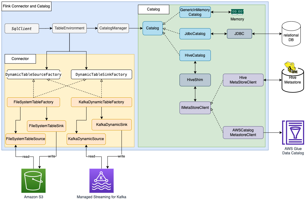
For data read/write, Flink has the interface DynamicTableSourceFactory for read and DynamicTableSinkFactory for write. A different Flink connector implements two interfaces to access data in different storage. For example, the Flink FileSystem connector has FileSystemTableFactory to read/write data in Hadoop Distributed File System (HDFS) or Amazon Simple Storage Service (Amazon S3), the Flink HBase connector has HBase2DynamicTableFactory to read/write data in HBase, and the Flink Kafka connector has KafkaDynamicTableFactory to read/write data in Kafka. You can refer to Table & SQL Connectors for more information.
For metadata read/write, Flink has the catalog interface. Flink has three built-in implementations for the catalog. GenericInMemoryCatalog stores the catalog data in memory. JdbcCatalog stores the catalog data in a JDBC-supported relational database. As of this writing, MySQL and PostgreSQL databases are supported in the JDBC catalog. HiveCatalog stores the catalog data in Hive Metastore. HiveCatalog uses HiveShim to provide different Hive version compatibility. We can configure different metastore clients to use Hive Metastore or the AWS Glue Data Catalog. In this post, we configure the Amazon EMR property hive.metastore.client.factory.class to com.amazonaws.glue.catalog.metastore.AWSGlueDataCatalogHiveClientFactory (see Using the AWS Glue Data Catalog as the metastore for Hive) so that we can use the AWS Glue Data Catalog to store Flink catalog data. Refer to Catalogs for more information.
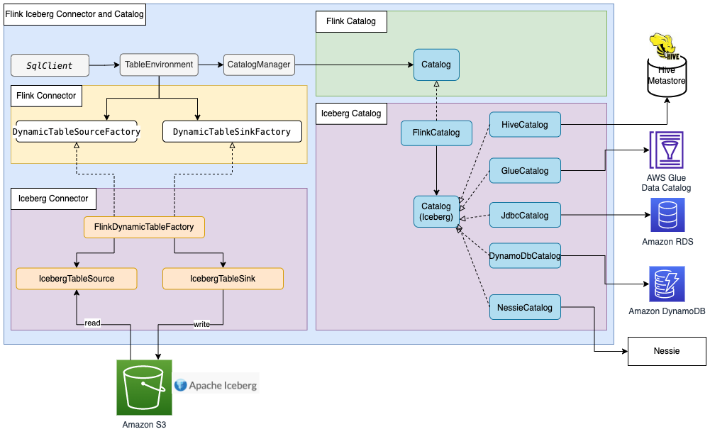
Most Flink built-in connectors, such as for Kafka, Amazon Kinesis, Amazon DynamoDB, Elasticsearch, or FileSystem, can use Flink HiveCatalog to store metadata in the AWS Glue Data Catalog. However, some connector implementations such as Apache Iceberg have their own catalog management mechanism. FlinkCatalog in Iceberg implements the catalog interface in Flink. FlinkCatalog in Iceberg has a wrapper to its own catalog implementation. The following diagram shows the relationship between Apache Flink, the Iceberg connector, and the catalog. For more information, refer to Creating catalogs and using catalogs and Catalogs.
Apache Hudi also has its own catalog management. Both HoodieCatalog and HoodieHiveCatalog implements a catalog interface in Flink. HoodieCatalog stores metadata in a file system such as HDFS. HoodieHiveCatalog stores metadata in Hive Metastore or the AWS Glue Data Catalog, depending on whether you configure hive.metastore.client.factory.class to use com.amazonaws.glue.catalog.metastore.AWSGlueDataCatalogHiveClientFactory. The following diagram shows relationship between Apache Flink, the Hudi connector, and the catalog. For more information, refer to Create Catalog.

Because Iceberg and Hudi have different catalog management mechanisms, we show three scenarios of Flink integration with the AWS Glue Data Catalog in this post:
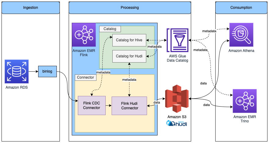
The following diagram shows the overall architecture of the solution described in this post.
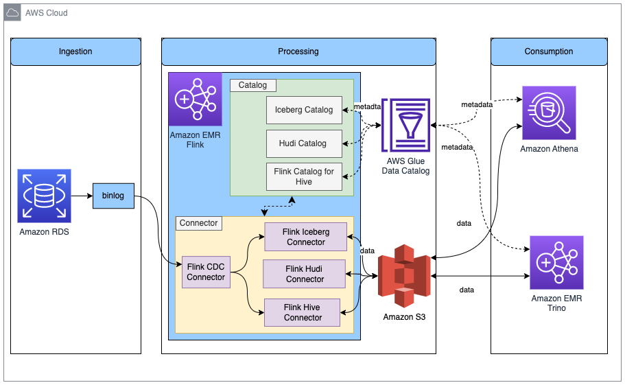
In this solution, we enable an Amazon RDS for MySQL binlog to extract transaction changes in real time. The Amazon EMR Flink CDC connector reads the binlog data and processes the data. Transformed data can be stored in Amazon S3. We use the AWS Glue Data Catalog to store the metadata such as table schema and table location. Downstream data consumer applications such as Amazon Athena or Amazon EMR Trino access the data for business analysis.
The following are the high-level steps to set up this solution:
binlog for Amazon RDS for MySQL and initialize the database.This post uses an AWS Identity and Access Management (IAM) role with permissions for the following services:
To enable CDC in Amazon RDS for MySQL, we need to configure binary logging for Amazon RDS for MySQL. Refer to Configuring MySQL binary logging for more information. We also create the database salesdb in MySQL and create the tables customer, order, and others to set up the data source.
binlog_format=ROW.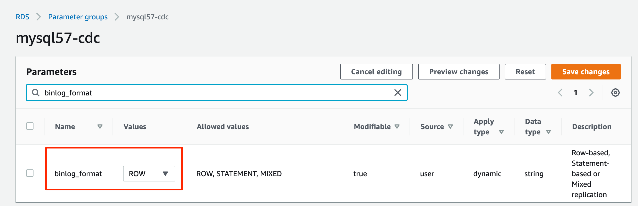
binlog_row_image=full.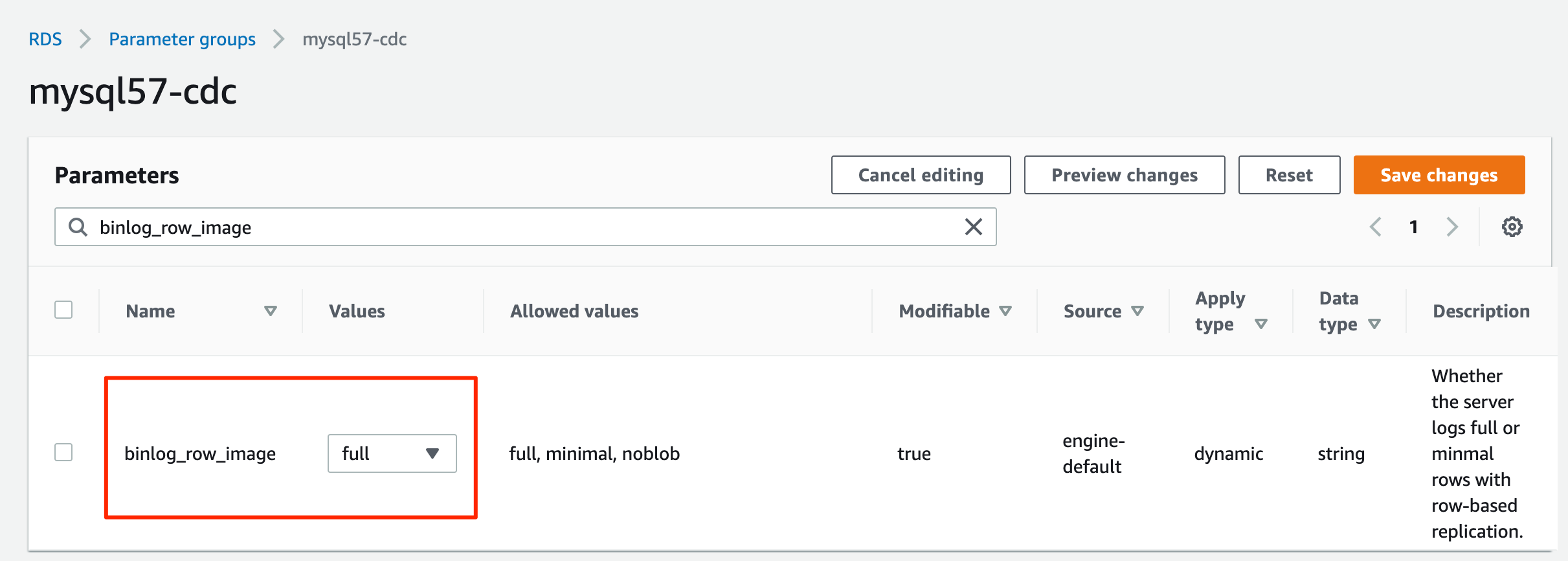
hostname, username, and password, which we use later.salesdb.sql command to initialize the database, providing the host name and user name according to your RDS for MySQL database configuration:From Amazon EMR 6.9.0, the Flink table API/SQL can integrate with the AWS Glue Data Catalog. To use the Flink and AWS Glue integration, you must create an Amazon EMR 6.9.0 or later version.
iceberg.properties for the Amazon EMR Trino integration with the Data Catalog. When the table format is Iceberg, your file should have following content:iceberg.properties to an S3 bucket, for example DOC-EXAMPLE-BUCKET.For more information on how to integrate Amazon EMR Trino with Iceberg, refer to Use an Iceberg cluster with Trino.
trino-glue-catalog-setup.sh to configure the Trino integration with the Data Catalog. Use trino-glue-catalog-setup.sh as the bootstrap script. Your file should have the following content (replace DOC-EXAMPLE-BUCKET with your S3 bucket name):trino-glue-catalog-setup.sh to your S3 bucket (DOC-EXAMPLE-BUCKET).Refer to Create bootstrap actions to install additional software to run a bootstrap script.
flink-glue-catalog-setup.sh to configure the Flink integration with the Data Catalog.flink-glue-catalog-setup.sh script as a step function.Your file should have the following content (the JAR file name here is using Amazon EMR 6.9.0; a later version JAR name may change, so make sure to update according to your Amazon EMR version).
Note that here we use an Amazon EMR step, not a bootstrap, to run this script. An Amazon EMR step script is run after Amazon EMR Flink is provisioned.
flink-glue-catalog-setup.sh to your S3 bucket (DOC-EXAMPLE-BUCKET).Refer to Configuring Flink to Hive Metastore in Amazon EMR for more information on how to configure Flink and Hive Metastore. Refer to Run commands and scripts on an Amazon EMR cluster for more details on running the Amazon EMR step script.
You can create an EMR cluster with the AWS Command Line Interface (AWS CLI) or the AWS Management Console. Refer to the appropriate subsection for instructions.
To use the AWS CLI, complete the following steps:
emr-flink-trino-glue.json to configure Amazon EMR to use the Data Catalog. Your file should have the following content:emr-flink-trino-glue.json parent folder path, S3 bucket, EMR cluster Region, EC2 key name, and S3 bucket for EMR logs.To use the console, complete the following steps:

s3://<region>.elasticmapreduce/libs/script-runner/script-runner.jar, where <region> is the region in which your EMR cluster resides.

The Flink CDC connector supports reading database snapshots and captures updates in the configured tables. We have deployed the Flink CDC connector for MySQL by downloading flink-sql-connector-mysql-cdc-2.2.1.jar and putting it into the Flink library when we create our EMR cluster. The Flink CDC connector can use the Flink Hive catalog to store Flink CDC table schema into Hive Metastore or the AWS Glue Data Catalog. In this post, we use the Data Catalog to store our Flink CDC table.
Complete the following steps to ingest RDS for MySQL databases and tables with Flink CDC and store metadata in the Data Catalog:
hive and providing your S3 bucket name:Because we’re configuring the EMR Hive catalog use the AWS Glue Data Catalog, all the databases and tables created in the Flink Hive catalog are stored in the Data Catalog.
Note that because the RDS for MySQL user name and password will be stored in the Data Catalog as table properties, you should be enable AWS Glue database/table authorization with AWS Lake Formation to protect your sensitive data.
You will get a query result like following screenshot.

As we’re ingesting the relational database data in Amazon RDS for MySQL, raw data may be updated or deleted. To support data update and delete, we can choose data lake technologies such as Apache Iceberg or Apache Hudi to store the processed data. As we mentioned earlier, Iceberg and Hudi have different catalog management. We show both scenarios to use Flink to read/write the Iceberg and Hudi tables with metadata in the AWS Glue Data Catalog.
For non-Iceberg and non-Hudi, we use a FileSystem Parquet file to show how the Flink built-in connector uses the Data Catalog.
The following diagram shows the architecture for this configuration.

catalog-impl as org.apache.iceberg.aws.glue.GlueCatalog.For more information about Flink and Data Catalog integration for Iceberg, refer to Glue Catalog.
The following diagram shows the architecture for this configuration.
Complete the following steps:
mode as hms.Because we already configured Amazon EMR to use the Data Catalog when we created the EMR cluster, this Hudi Hive catalog uses the Data Catalog under the hood. For more information about Flink and Data Catalog integration for Hudi, refer to Create Catalog.
The following diagram shows the architecture for this configuration.
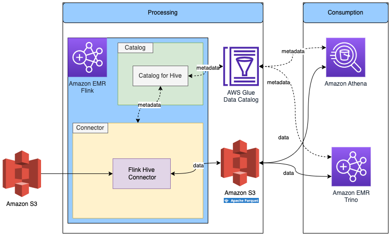
We already created the Flink Hive catalog in the previous step, so we’ll reuse that catalog.
We change the SQL dialect to Hive to create a table with Hive syntax.
Because Parquet files don’t support updated rows, we can’t consume data from CDC data. However, we can consume data from Iceberg or Hudi.
You can navigate to the AWS Glue console to verify all the tables are stored in the Data Catalog.


You can use Athena or Amazon EMR Trino to access the result data.
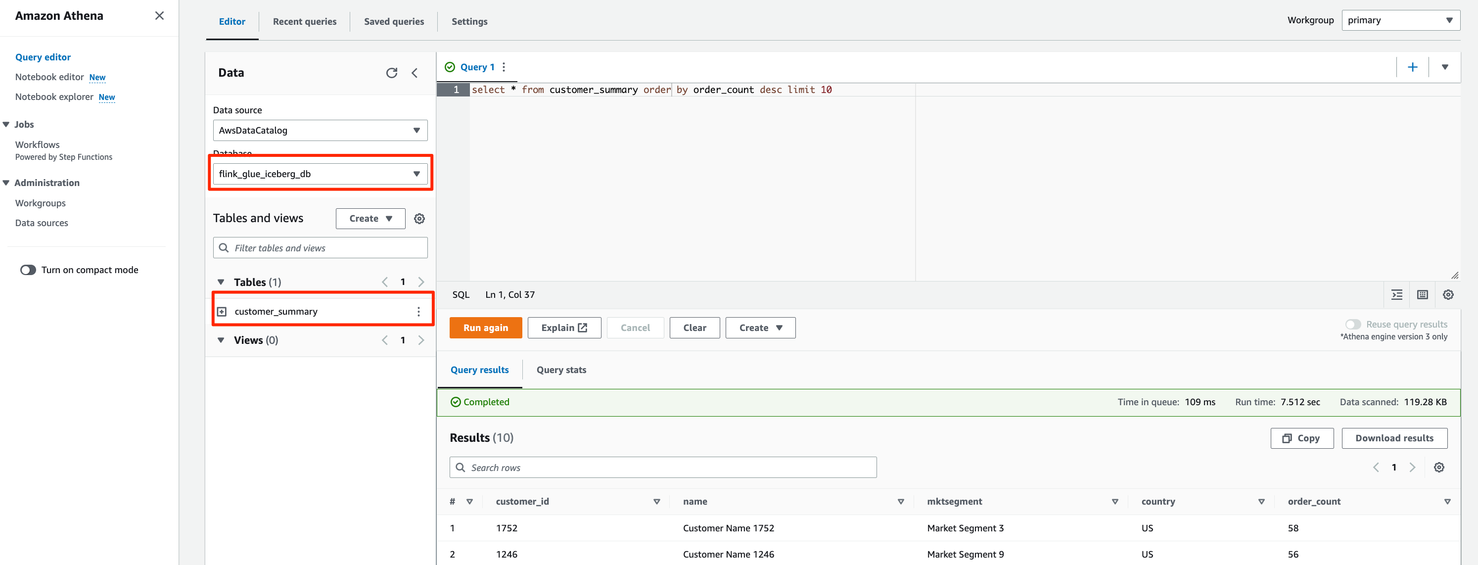
To access the data with Athena, complete the following steps:
flink_glue_iceberg_db for Database.You should see the customer_summary table listed.
The query result will look like the following screenshot.
flink_glue_hudi_db and run the same SQL query.
flink_hive_parquet_db and run the same SQL query.
To access Iceberg with Amazon EMR Trino, SSH to the EMR primary node.
Amazon EMR Trino can now query the tables in the AWS Glue Data Catalog.
The query result looks like the following screenshot.

hive catalog to query the Hudi table:We can update and delete some records in the RDS for MySQL database and then validate that the changes are reflected in the Iceberg and Hudi tables.
customer_summary table with Athena or Amazon EMR Trino.The updated and deleted records are reflected in the Iceberg and Hudi tables.

When you’re done with this exercise, complete the following steps to delete your resources and stop incurring costs:
This post showed you how to integrate Apache Flink in Amazon EMR with the AWS Glue Data Catalog. You can use a Flink SQL connector to read/write data in a different store, such as Kafka, CDC, HBase, Amazon S3, Iceberg, or Hudi. You can also store the metadata in the Data Catalog. The Flink table API has the same connector and catalog implementation mechanism. In a single session, we can use multiple catalog instances pointing to different types, like IcebergCatalog and HiveCatalog, and use then interchangeably in your query. You can also write code with the Flink table API to develop the same solution to integrate Flink and the Data Catalog.
In our solution, we consumed the RDS for MySQL binary log directly with Flink CDC. You can also use Amazon MSK Connect to consume the binary log with MySQL Debezim and store the data in Amazon Managed Streaming for Apache Kafka (Amazon MSK). Refer to Create a low-latency source-to-data lake pipeline using Amazon MSK Connect, Apache Flink, and Apache Hudi for more information.
With the Amazon EMR Flink unified batch and streaming data processing function, you can ingest and process data with one computing engine. With Apache Iceberg and Hudi integrated in Amazon EMR, you can build an evolvable and scalable data lake. With the AWS Glue Data Catalog, you can manage all enterprise data catalogs in a unified manner and consume data easily.
Follow the steps in this post to build your unified batch and streaming solution with Amazon EMR Flink and the AWS Glue Data Catalog. Please leave a comment if you have any questions.
 Jianwei Li is Senior Analytics Specialist TAM. He provides consultant service for AWS enterprise support customers to design and build modern data platform.

Samrat Deb is Software Development Engineer at Amazon EMR. In his spare time, he love exploring new places, different culture and food.

Prabhu Josephraj is a Senior Software Development Engineer working for Amazon EMR. He is focused on leading the team that builds solutions in Apache Hadoop and Apache Flink. In his spare time, Prabhu enjoys spending time with his family.
Post Syndicated from Bruce Schneier original https://www.schneier.com/blog/archives/2023/01/kevin-mitnick-hacked-california-law-in-1983.html
Early in his career, Kevin Mitnick successfully hacked California law. He told me the story when he heard about my new book, which he partially recounts his 2012 book, Ghost in the Wires.
The setup is that he just discovered that there’s warrant for his arrest by the California Youth Authority, and he’s trying to figure out if there’s any way out of it.
As soon as I was settled, I looked in the Yellow Pages for the nearest law school, and spent the next few days and evenings there poring over the Welfare and Institutions Code, but without much hope.
Still, hey, “Where there’s a will…” I found a provision that said that for a nonviolent crime, the jurisdiction of the Juvenile Court expired either when the defendant turned twenty-one or two years after the commitment date, whichever occurred later. For me, that would mean two years from February 1983, when I had been sentenced to the three years and eight months.
Scratch, scratch. A little arithmetic told me that this would occur in about four months. I thought, What if I just disappear until their jurisdiction ends?
This was the Southwestern Law School in Los Angeles. This was a lot of manual research—no search engines in those days. He researched the relevant statutes, and case law that interpreted those statutes. He made copies of everything to hand to his attorney.
I called my attorney to try out the idea on him. His response sounded testy: “You’re absolutely wrong. It’s a fundamental principle of law that if a defendant disappears when there’s a warrant out for him, the time limit is tolled until he’s found, even if it’s years later.”
And he added, “You have to stop playing lawyer. I’m the lawyer. Let me do my job.”
I pleaded with him to look into it, which annoyed him, but he finally agreed. When I called back two days later, he had talked to my Parole Officer, Melvin Boyer, the compassionate guy who had gotten me transferred out of the dangerous jungle at LA County Jail. Boyer had told him, “Kevin is right. If he disappears until February 1985, there’ll be nothing we can do. At that point the warrant will expire, and he’ll be off the hook.”
So he moved to Northern California and lived under an assumed name for four months.
What’s interesting to me is how he approaches legal code in the same way a hacker approaches computer code: pouring over the details, looking for a bug—a mistake—leading to an exploitable vulnerability. And this was in the days before you could do any research online. He’s spending days in the law school library.
This is exactly the sort of thing I am writing about in A Hacker’s Mind. Legal code isn’t the same as computer code, but it’s a series of rules with inputs and outputs. And just like computer code, legal code has bugs. And some of those bugs are also vulnerabilities. And some of those vulnerabilities can be exploited—just as Mitnick learned.
Mitnick was a hacker. His attorney was not.
Post Syndicated from Ankur Taunk original https://aws.amazon.com/blogs/big-data/advance-reporting-and-analytics-for-the-post-call-analytics-pca-solution-with-amazon-quicksight/
Organizations with contact centers benefit from advanced analytics on their call recordings to gain important product feedback, improve contact center efficiency, and identify coaching opportunities for their staff. The Post Call Analytics (PCA) solution uses AWS machine learning (ML) services like Amazon Transcribe and Amazon Comprehend to extract insights from contact center call audio recordings uploaded after the call, or from integration with our companion Live Call Analytics (LCA) solution. You can visualize the PCA insights in the business intelligence (BI) tool Amazon QuickSight for advanced analysis.
In this post, we show you how to use PCA’s data to build automated QuickSight dashboards for advanced analytics to assist in quality assurance (QA) and quality management (QM) processes. We provide an AWS CloudFormation template and step-by-step instructions, allowing you to get started with our sample dashboard in just a few simple steps.
The following screenshots illustrate the different components of our sample QuickSight dashboard:


The solution uses the following AWS services and features:
The following architecture diagram shows how our solution uses PCA insights from a call recording in an S3 bucket to enable analytics in QuickSight.

As part of the solution workflow, EventBridge receives an event for each PCA solution analysis output file. Kinesis Data Firehose uses Lambda to perform data transformation and compression, storing the file in a compressed columnar format (Parquet) in the target S3 bucket. The AWS Glue Data Catalog has the table definitions for the data sources. Athena runs queries using a variety of SQL statements on the compressed Parquet files, and QuickSight is used for visualization. To optimize query performance, we use Athena partition projections. This feature automatically creates date-based partitions for query performance and cost optimization.
This is a loosely coupled architecture, with flexibility to ingest data from third-party data sources, enrich the data by adding more data points, and cross-reference data across data sources for your analytics use case. Lambda functions can integrate with third-party data sources to process and store the compressed output in Amazon S3 using Kinesis Data Firehose. Athena lets you create views by cross-referencing the data across multiple tables.
You should have the following prerequisites:
Note that this solution uses QuickSight SPICE storage.
To deploy the solution, complete the following steps:
OutputBucket.
OutputBucket:
OutputBucket (ref. step 3) on the Amazon S3 console.pca-quicksight-analytics).OutputBucket. (ref. step 3)WebAppUrl output from your PCA stack.
<Stack Name>-PCA-Dashboard and choose Share.<Stack Name>-PCA-Analysis under Asset type analyses and <Stack Name>-PCA-* under Datasets.After you deploy the solution, you can explore the dashboards by loading demo data.
OutputBucket bucket in the /parsedFiles/ folder.Note that this step is optional. We recommend using a non-production environment or stack to keep production and demo data segregated.
Once deployed, the solution processes new PCA data as it is added. To process older PCA data, complete the following steps:
OutputBucket on the Amazon S3 console./parsedFiles/ folder.This triggers an EventBridge rule to process the historical PCA files and stream the data to the QuickSight dashboard.
After you generate the PCA output data (within a few minutes), a compressed Parquet PCA data file will appear in the PCA OutputBucket under pca-output-base.
pca database. You should see the pca_output table under Tables and views.pca_output table and choose Preview Table.

FromDate and ToDate to view older data or a custom time frame.To remove the resources created by this stack, perform the following steps:
OutputBucket bucket under /parsedFiles/.pca-output-base folder under the PCA output bucket.In this post, you learned how to visualize PCA solution data, using a CloudFormation template to automate the QuickSight dashboard creation. You also learned to how to visualize historical PCA data in QuickSight.
The sample PCA QuickSight dashboard application is provided as open source—use it as a starting point for your own solution, and help us make it better by contributing back fixes and features via GitHub pull requests. For expert assistance, AWS Professional Services and other AWS Partners are here to help.
 Mehmet Demir is a Senior Solutions Architect at Amazon Web Services (AWS) based in Toronto, Canada. He helps customers in building well-architected solutions that support business innovation.
 Ankur Taunk is a Senior Specialist Solutions Architect at AWS. He helps customer achieve their desired business outcomes in the Contact Center space leveraging Amazon Connect.
Post Syndicated from Brendan Jenkins original https://aws.amazon.com/blogs/devops/deliver-operational-insights-to-atlassian-opsgenie-using-devops-guru/
As organizations continue to grow and scale their applications, the need for teams to be able to quickly and autonomously detect anomalous operational behaviors becomes increasingly important. Amazon DevOps Guru offers a fully managed AIOps service that enables you to improve application availability and resolve operational issues quickly. DevOps Guru helps ease this process by leveraging machine learning (ML) powered recommendations to detect operational insights, identify the exhaustion of resources, and provide suggestions to remediate issues. Many organizations running business critical applications use different tools to be notified about anomalous events in real-time for the remediation of critical issues. Atlassian is a modern team collaboration and productivity software suite that helps teams organize, discuss, and complete shared work. You can deliver these insights in near-real time to DevOps teams by integrating DevOps Guru with Atlassian Opsgenie. Opsgenie is a modern incident management platform that receives alerts from your monitoring systems and custom applications and categorizes each alert based on importance and timing.
This blog post walks you through how to integrate Amazon DevOps Guru with Atlassian Opsgenie to
receive notifications for new operational insights detected by DevOps Guru with more flexibility and customization using Amazon EventBridge and AWS Lambda. The Lambda function will be used to demonstrate how to customize insights sent to Opsgenie.
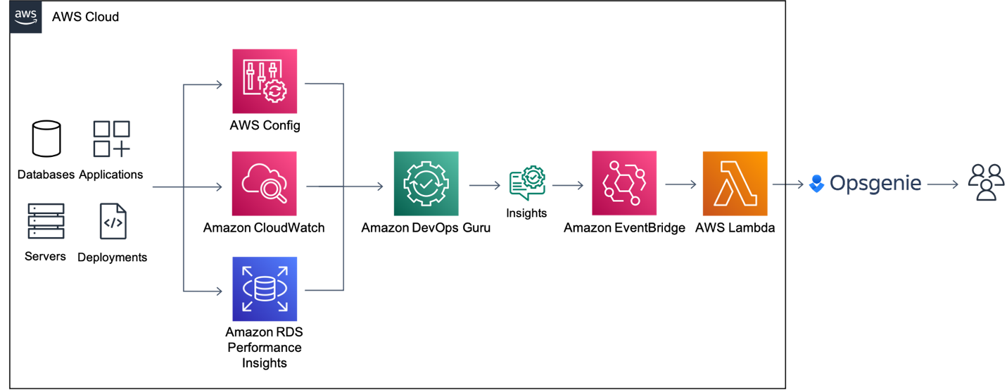
Figure 1: Amazon EventBridge Integration with Opsgenie using AWS Lambda
Amazon DevOps Guru directly integrates with Amazon EventBridge to notify you of events relating to generated insights and updates to insights. To begin routing these notifications to Opsgenie, you can configure routing rules to determine where to send notifications. As outlined below, you can also use pre-defined DevOps Guru patterns to only send notifications or trigger actions that match that pattern. You can select any of the following pre-defined patterns to filter events to trigger actions in a supported AWS resource. Here are the following predefined patterns supported by DevOps Guru:
By default, the patterns referenced above are enabled so we will leave all patterns operational in this implementation. However, you do have flexibility to change which of these patterns to choose to send to Opsgenie. When EventBridge receives an event, the EventBridge rule matches incoming events and sends it to a target, such as AWS Lambda, to process and send the insight to Opsgenie.
The following prerequisites are required for this walkthrough:
In this tutorial, you will perform the following steps:
In this step, you will navigate to Opsgenie to create the integration with DevOps Guru and to obtain the API key and team name within your account. These parameters will be used as inputs in a later section of this blog.
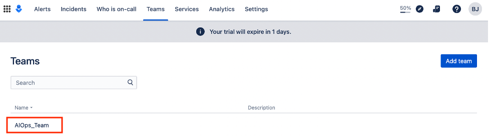
Figure 2: Opsgenie team names
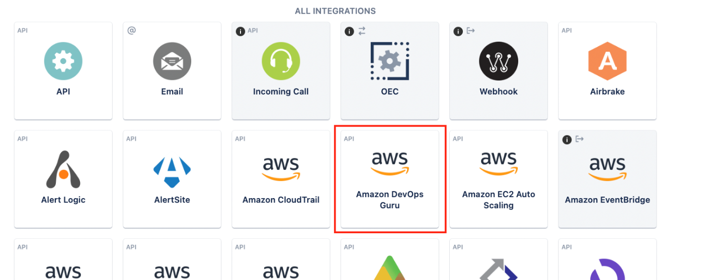
Figure 3: Integration option for DevOps Guru
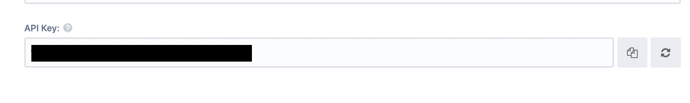
Figure 4: API Key for DevOps Guru Integration
In this step, you will review & launch the SAM template. The template will deploy an AWS Lambda function that is triggered by an Amazon EventBridge rule when Amazon DevOps Guru generates a new event. The Lambda function will retrieve the parameters obtained from the deployment and pushes the events to Opsgenie via an API.
Below is the SAM template that will be deployed in the next step. This template launches a few key components specified earlier in the blog. The Transform section of the template allows us takes an entire template written in the AWS Serverless Application Model (AWS SAM) syntax and transforms and expands it into a compliant CloudFormation template. Under the Resources section this solution will deploy an AWS Lamba function using the Java runtime as well as an Amazon EventBridge Rule/Pattern. Another key aspect of the template are the Parameters. As shown below, the ApiKey, Email, and TeamName are parameters we will use for this CloudFormation template which will then be used as environment variables for our Lambda function to pass to OpsGenie.
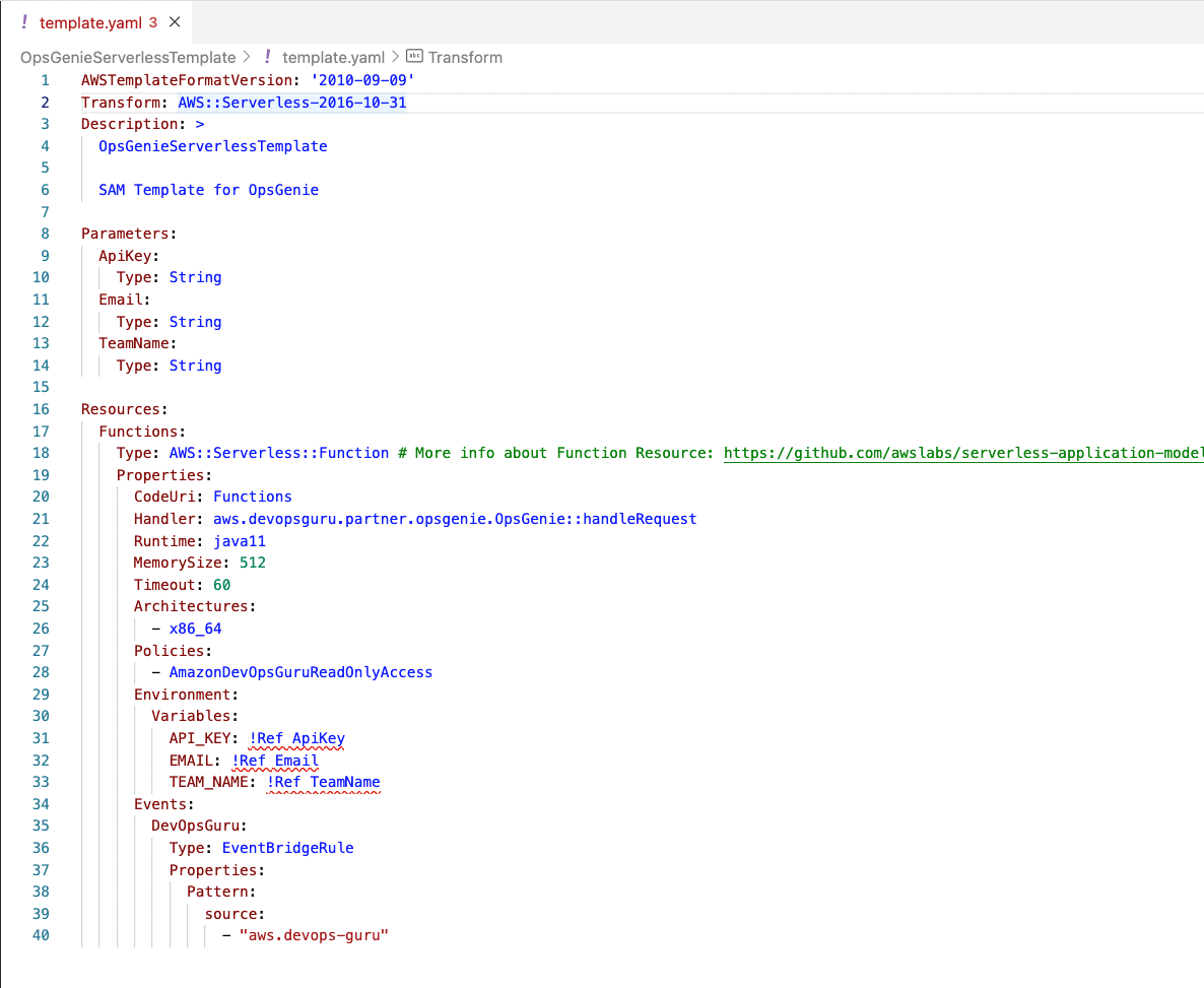
Figure 5: Review of SAM Template
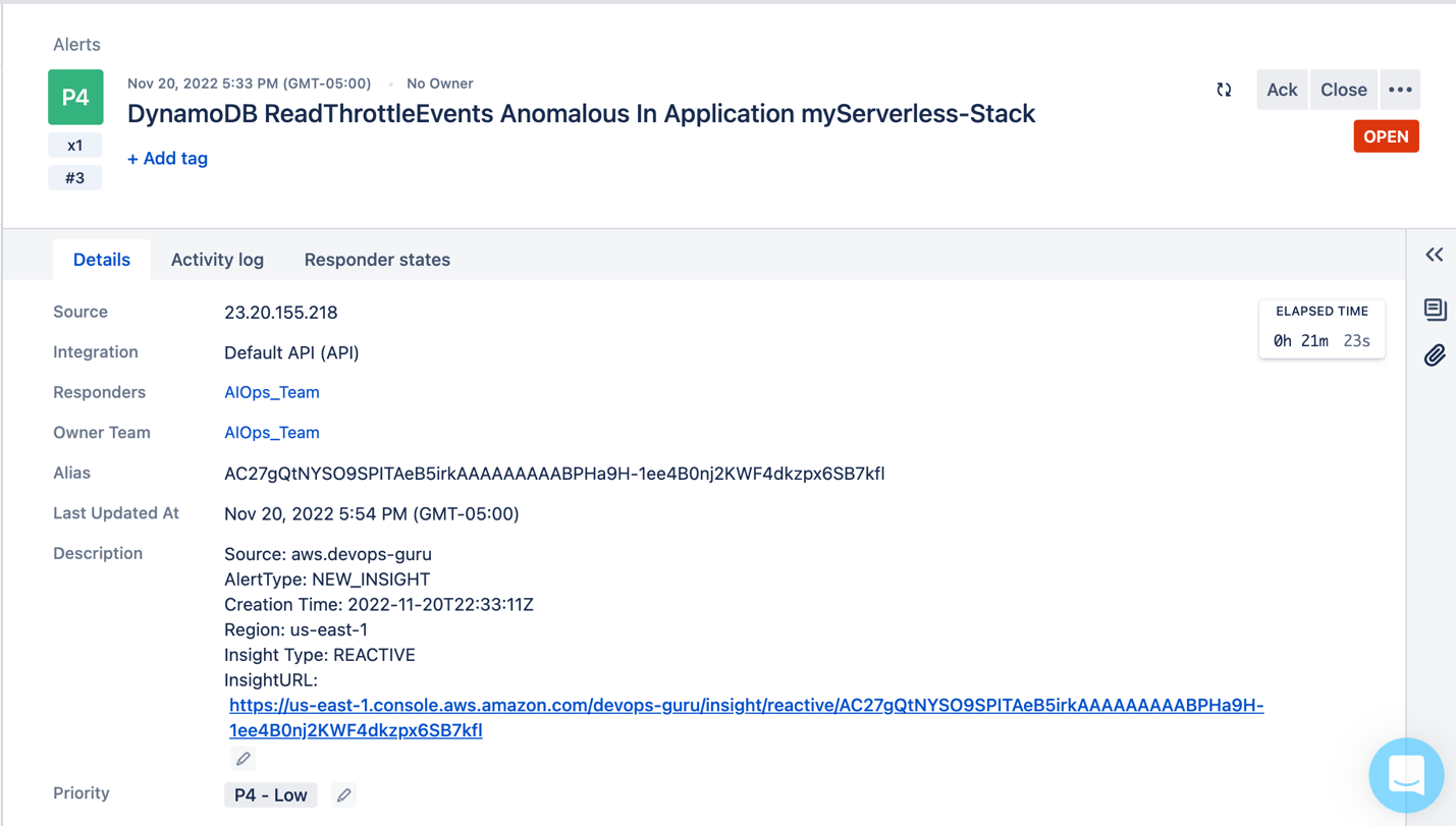
Figure 6: Event Published to Opsgenie with details such as the source, alert type, insight type, and a URL to the insight in the AWS console.enecccdgruicnuelinbbbigebgtfcgdjknrjnjfglclt
To avoid incurring future charges, delete the resources.
The foundation of the DevOps Guru and Opsgenie integration is based on Amazon EventBridge and AWS Lambda which allows you the flexibility to implement several customizations. An example of this would be the ability to generate an Opsgenie alert when a DevOps Guru insight severity is high. Another example would be the ability to forward appropriate notifications to the AIOps team when there is a serverless-related resource issue or forwarding a database-related resource issue to your DBA team. This section will walk you through how these customizations can be done.
EventBridge rules can be used to select specific events by using event patterns. As detailed below, you can trigger the lambda function only if a new insight is opened and the severity is high. The advantage of this kind of customization is that the Lambda function will only be invoked when needed.
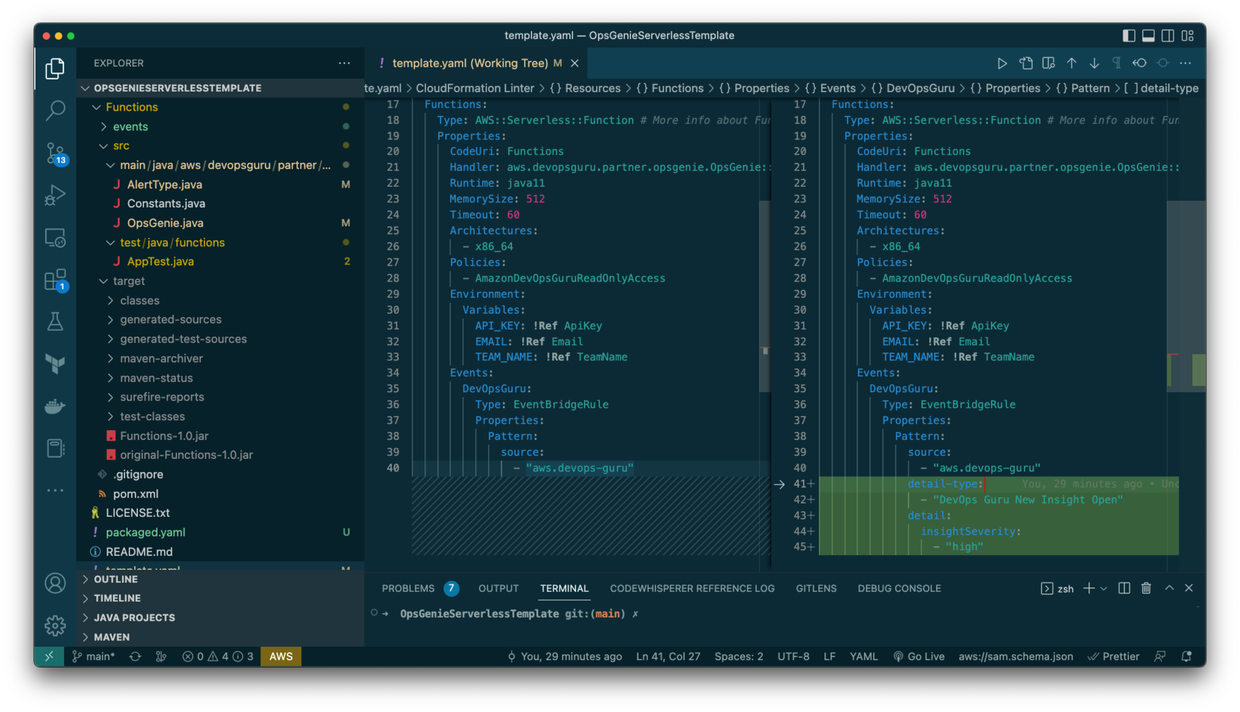
Figure 7: CloudFormation template file changed so that the EventBridge rule is only triggered when the alert type is “DevOps Guru New Insight Open” and insightSeverity is “high”.
Another customization would be to change the Lambda code to route and control how alerts will be managed. Let’s say you want to get your DBA team involved whenever DevOps Guru raises an insight related to an Amazon RDS resource. You can change the AlertType Java class as follows:
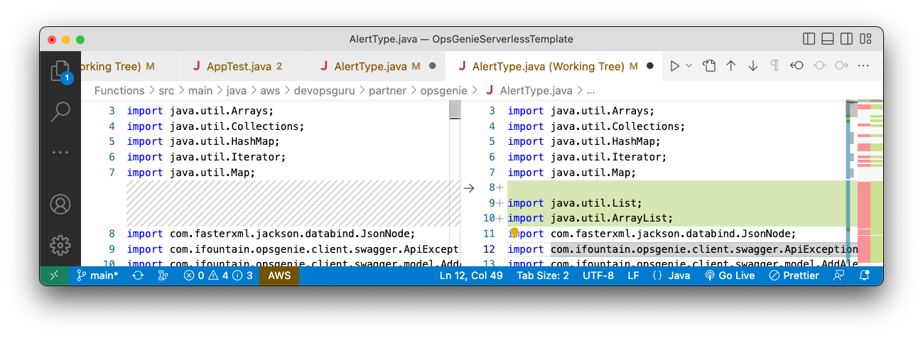
Figure 8: java.util.List and java.util.ArrayList packages were imported
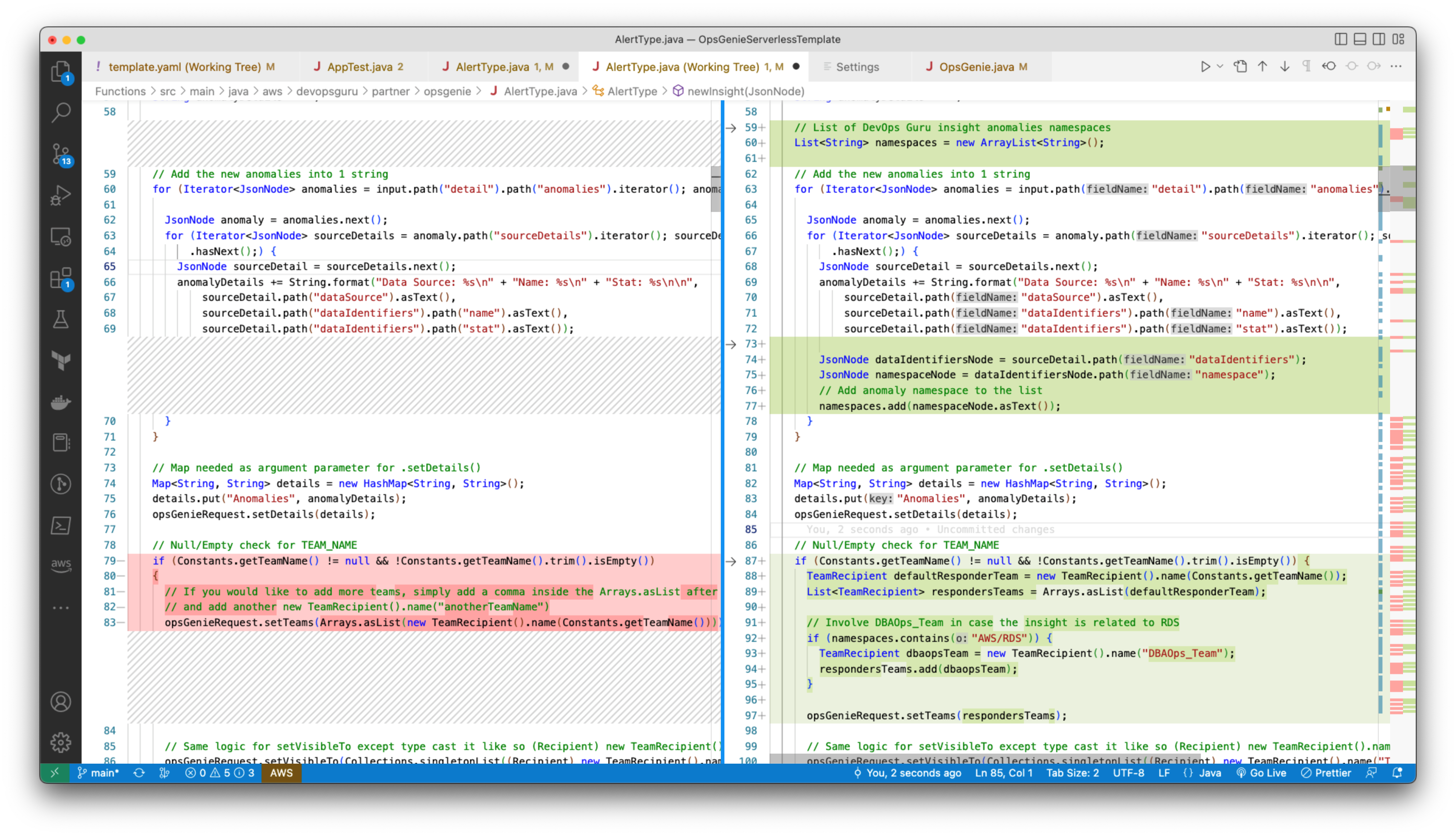
Figure 9: AlertType Java class customized to include DBAOps_Team for RDS-related DevOps Guru insights.
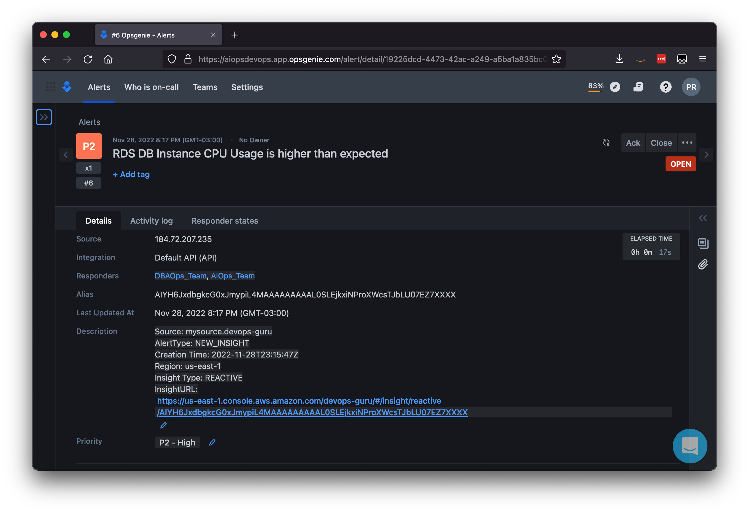
Figure 10: Opsgenie alert assigned to both DBAOps_Team and AIOps_Team.
In this post, you learned how Amazon DevOps Guru integrates with Amazon EventBridge and publishes insights to Opsgenie using AWS Lambda. By creating an Opsgenie integration with DevOps Guru, you can now leverage Opsgenie strengths, incident management, team communication, and collaboration when responding to an insight. All of the insight data can be viewed and addressed in Opsgenie’s Incident Command Center (ICC). By customizing the data sent to Opsgenie via Lambda, you can empower your organization even more by fine tuning and displaying the most relevant data thus decreasing the MTTR (mean time to resolve) of the responding operations team.
About the authors:
Post Syndicated from Vidya Kotamraju original https://aws.amazon.com/blogs/big-data/diligent-enhances-customer-governance-with-automated-data-driven-insights-using-amazon-quicksight/
This post is co-written with Vidya Kotamraju and Tallis Hobbs, from Diligent.
Diligent is the global leader in modern governance, providing software as a service (SaaS) services across governance, risk, compliance, and audit, helping companies meet their environmental, social, and governance (ESG) commitments. Serving more than 1 million users from over 25,000 customers around the world, we empower transformational leaders with software, insights, and confidence to drive greater impact and lead with purpose.
We provide the right governance technology that empowers our customers to act strategically while maintaining compliance, mitigating risk, and driving efficiency. With the Diligent Platform, organizations can bring their most critical data into one centralized place. By using powerful analytics, automation, and unparalleled industry data, our customers’ board and c-suite get relevant insights from across risk, compliance, audit, and ESG teams that help them make better decisions, faster and more securely.
One of the biggest obstacles that customers face is obtaining a holistic view of their data. To effectively manage risks and ensure compliance, organizations need to have a comprehensive understanding of their operations and processes. However, this can be difficult to achieve. Scenarios such as data being dispersed across multiple systems and departments, or if data is not consistently collected and updated, or if data is not in a format that can be easily analyzed can all present various challenges. To address them, we turned to Amazon QuickSight to enhance our customer-facing products with embedded insights and reports.
In this post, we cover what we were looking for in a business intelligence (BI) tool, and how QuickSight met our requirements.
To effectively serve our customers, we needed a platform-wide reporting solution that would enable our users to centralize their governance, risk, and compliance (GRC) programs, and collect information from disparate data sources, while allowing for integrated automation and analytics for data-driven insights, thereby providing a curated picture of GRC with confidence.
When we started our research into various BI tool offerings to embed into our platform, we narrowed the list down to a handful that had most of the capabilities we were looking for. After reviewing the options, QuickSight was our top option when it came to the ease of integration with our existing AWS-built ecosystem. QuickSight offered everything we needed, with the flexibility we wanted, at an affordable price.
There are many data points that can be useful for making business decisions; the specific data points that are most critical will depend on the nature of the business and the decisions being made. However, there are some common types of data that are often important for making informed business decisions: financial data, marketing data, operational data, and customer data.
Translating those requirements into BI tool functionality, we were looking for:
QuickSight checked all the boxes on our list. The most compelling reasons why we ultimately chose QuickSight were:
Today, we’re using Quicksight to create a customer-facing reporting platform that allows our customers to report on their data within our ecosystem. QuickSight helps empower our customers by putting the reporting tools and capability in their hands, allowing them to get a comprehensive, personalized (via row-level security) view of data, unique to their workflow.
The following screenshot shows an example of our Issues & Actions dashboard, designed for risk managers and audit managers, showing various issues in need of attention.

QuickSight has provided a way to enable our customers to bring data and intelligence to the board or leadership teams in a simple, more streamlined way that saves time and effort—by automating standard reporting and surfacing it in a rich and interactive dashboard for directors. Boards and leaders will have access to curated insights, culled from both internal operations and external sources, integrated into the Diligent Boards platform—visualized in such a way that their data tells the story that accompanies the board materials.
For us, the most compelling benefit of using QuickSight is the ease of integration with Diligent’s existing tech stack and data stack. Quicksight integrates seamlessly with other AWS products in our technology stack, making it easy to incorporate data from various sources and systems into our dashboards and reports.
Our customers love the flexibility with reporting. Quicksight provides a range of visualization options that allows users to customize their dashboards and reports to fit their specific needs and preferences. We love that the QuickSight team is open to taking prompt action on customer feedback. Their continuous and frequent feature release process is confidence-inspiring.
QuickSight helps us provide flexibility to our customers, enabling them to quickly put the right data in front of the right audience to make the right business decisions.
To learn more, visit Amazon QuickSight.
 Vidya Kotamraju is a Product Management Leader at Diligent, with close to 2 decades of experience leading award-winning B2B, B2C product and team success across multiple industries and geographies. Currently, she is focused on Diligent Highbond’s Data Automation Solutions.
 Tallis Hobbs is a Senior Software Engineer at Diligent. As a previous educator, he brings a unique skill set to the engineering space. He is passionate about the AWS serverless space and currently works on Diligent’s client facing Quicksight integration.
 Samit Kumbhani is a Sr. Solutions Architect at AWS based out of New York City area. Has has 18+ years of experience in building applications and focuses on Analytics, Business Intelligence and Databases. He enjoys working with customers to understand their challenges and solve them by creating innovative solutions using AWS services. Outside of work, Samit loves playing cricket, traveling and spending time with his family and friends.
Post Syndicated from Backblaze original https://www.backblaze.com/blog/extended-maintenance-window-for-us-west-data-center/
On Wednesday, February 1, at 8:00 a.m. PT (4:00 p.m. UTC), we’ll be performing planned maintenance on a data center in our U.S. West data region. We expect the work to take place over four to eight hours. During the window, we do not anticipate any service impacts outside of what customers typically experience during our standard scheduled maintenance. The maintenance is only being performed on one data center in the U.S. West data region. Customers with data stored in this region should see minimal to no impact beyond what is listed below.
Most services, including Computer Backup uploads and most B2 Cloud Storage operations (i.e., uploads, downloads, listing, key creation) will function normally. Within the maintenance window, some customers may experience interruptions of four hours to eight hours in the following areas:
Web Interface:
Computer Backup:
B2 Cloud Storage:
If timing or impacts change materially—which we do not expect to occur—we will endeavor to offer updates on our social media channels. If you have any questions, you can contact our Support Team through the Help page.
The post Extended Maintenance Window for US West Data Center appeared first on Backblaze Blog | Cloud Storage & Cloud Backup.
Post Syndicated from original https://lwn.net/Articles/921487/
Version
1.67.0 of the Rust language has been released. The list of new
features is relatively short; it includes support for #[must_use]
on async functions and a new multi-producer, single-consumer channel
implementation.
Post Syndicated from original https://lwn.net/Articles/920891/
Memory allocation within the kernel is a complex business. The amount of
physical memory available on any given system will be strictly limited,
meaning that an allocation request can often only be satisfied by taking
memory from somebody else, but some of the options for reclaiming memory
may not be available when a request is made. Additionally,
some allocation requests have
requirements dictating where that memory can be placed or how quickly the
allocation must be made. The kernel’s
memory-allocation functions have long supported a set of “GFP flags” used
to describe the requirements of each specific request. Those flags will
probably undergo some changes soon as the result of this
patch set posted by Mel Gorman; that provides an opportunity to look at
those flags in some detail.
Post Syndicated from original https://lwn.net/Articles/921477/
Security updates have been issued by Debian (bind9, chromium, and modsecurity-apache), Fedora (libgit2, mediawiki, and redis), Oracle (go-toolset:ol8, java-1.8.0-openjdk, systemd, and thunderbird), Red Hat (java-1.8.0-openjdk and redhat-ds:12), SUSE (apache2, bluez, chromium, ffmpeg-4, glib2, haproxy, kernel, libXpm, podman, python-py, python-setuptools, samba, xen, xrdp, and xterm), and Ubuntu (samba).
Post Syndicated from Sebastian Hufnagel original https://blog.cloudflare.com/towards-a-global-framework-for-cross-border-data-flows-and-privacy-protection/


As our societies and economies rely more and more on digital technologies, there is an increased need to share and transfer data, including personal data, over the Internet. Cross-border data flows have become essential to international trade and global economic development. In fact, the digital transformation of the global economy could never have happened as it did without the open and global architecture of the Internet and the ability for data to transcend national borders. As we described in our blog post yesterday, data localization doesn’t necessarily improve data privacy. Actually, there can be real benefits to data security and – by extension – privacy if we are able to transfer data across borders. So with Data Privacy Day coming up tomorrow, we wanted to take this opportunity to drill down into the current environment for the transfer of personal data from the EU to the US, which is governed by the EU’s privacy regulation (GDPR). Looking to the future, we will make the case for a more stable, global cross-border data transfer framework, which will be critical for an open, more secure and more private Internet.
In the last decade, we have observed a growing tendency around the world to ring-fence the Internet and erect new barriers to international data flows, especially personal data. In some cases this has resulted in less choice and poorer performance for users of digital products and services. In other cases it has limited free access to information, and – paradoxically- in some cases this has resulted in even less data security and privacy, which is contrary to the very rationale of data protection regulations. The motives for these concerning developments are manifold, ranging from a lack of trust with regard to privacy protection in third countries, to asserting national security, to seeking economic self-determination.
In the European Union, for the last few years, even the most privacy-focused companies (like Cloudflare) have faced a drumbeat of speculation and concerns from some hardliner data protection authorities, privacy activists and others about whether data processed by US cloud service providers could really be processed in a manner that complies with the GDPR. Often, these concerns are purely legalistic and fail to take into account the actual risks associated with a specific data transfer, and, in Cloudflare’s case, the essential contribution of our services to the security and privacy of millions of European Internet users. In fact, official guidance from the European Data Protection Board (EDPB) has confirmed that EU personal data can still be processed in the US, but this has become quite complicated since the suspension of the Privacy Shield framework by the European Court of Justice with its 2020 Schrems II judgment: data controllers must use legal transfer mechanisms such as EU standard contractual clauses as well as a host of additional legal, technical and organizational safeguards.
However, it is ultimately up to the competent data protection authorities to decide whether such measures are sufficient in a case-by-case interpretation. Since these cases are often quite complex, since every case is different, and since there are 45 data protection authorities across Europe alone, this approach simply doesn’t scale. Further, DPAs – sometimes even within the same EU country (Germany) – have disagreed in their interpretation of the law when it comes to third country transfers. And when it comes to an actual court ruling, it is our experience that the courts tend to be more pragmatic and balanced about data protection than the DPAs are. But it takes a long time and many resources before a data protection case ends up before a court. This is particularly problematic for small businesses that can’t afford lengthy legal battles. As a result, the theoretical threat of a hefty fine from a DPA may create enough of a deterrent for them to stop using services involving third-country data transfers altogether, even if those services provide greater security and privacy for the personal data they process, and make them more productive. This is clearly not in the interest of the European economy and most likely was not the intention of policy-makers when adopting the GDPR back in 2016.
While recent developments will not resolve all the challenges mentioned above, last December, after years of complex negotiations, international policy-makers took two important steps towards restoring legal certainty and trust relating to cross-border flows of personal data.
On December 13, 2022, the European Commission published its long-awaited preliminary assessment that the EU would consider that personal data transferred from the EU to the US under the future EU-US Data Privacy Framework (DPF) enjoys an adequate level of protection in the United States. The assessment follows the recent signing of Executive Order 14086 by US President Biden, which comprehensively addressed the concerns expressed by the European Court of Justice (ECJ) in its 2022 Schrems II decision. Notably, the US government will impose additional limits on US authorities’ use of bulk surveillance methods against non-US citizens and create an independent redress mechanism in the US that allows EU data subjects to exercise their data protection rights. While the Commission’s initial assessment is only the start of an EU ratification process that is expected to take about 4-6 months, experts are very optimistic that it will be adopted at the end.
Just one day later, the US, along with the 37 other OECD countries and the European Union, adopted a first-of-its kind agreement to enhance trust in cross-border data flows between rule-of law democratic systems, by articulating joint principles for safeguards to protect privacy and other human rights and freedoms when governments access personal data held by private entities on grounds of national security and law enforcement. Where legal frameworks require that transborder data flows are subject to safeguards, like in the case of GDPR in the EU, participants agreed to “take into account a destination country’s effective implementation of the principles as a positive contribution towards facilitating transborder data flows in the application of those rules.” (It’s also good to note that, in line with Cloudflare’s mission to help build a better Internet, the OECD declaration recalls members’ shared commitment to a “global, open, accessible, interconnected, interoperable, reliable and secure Internet”).
The EU-US DPF and the OECD Declaration are complementary to each other and both mark important steps to restore trust in cross-border data flows between countries that share common values like democracy and the rule of law, protecting privacy and other human rights and freedoms. However, both approaches come with their own limitations: the DPF is limited to personal data transfers from the EU to the US In addition, it cannot be excluded that it will be invalidated by the ECJ again in a few years time, as privacy activists have already announced that they will legally challenge it again. The OECD Declaration, on the other hand, is global in scope, but limited to general principles for governments, which can be interpreted quite differently in practice.
This is why, in addition to these efforts, we need a stable, multilateral framework with specific privacy protection requirements, which cannot be invalidated unilaterally. One single global certification should suffice for participating companies to safely transfer personal data between participating countries worldwide. The emerging Global Cross Border Privacy Rules (CBPR) certification, which is already supported by several governments from North America and Asia, looks very promising in this regard.
European policy-makers will ultimately need to decide whether they want to continue on the present path, which risks leaving Europe behind as an isolated data island. Alternatively, the EU could revise its privacy regulation with a view to prevent Europe’s many national and regional data protection authorities from interpreting it in a way that is out of touch with reality. It could also make it interoperable with a global framework for cross-border data flows based on shared values and mutual trust.
Cloudflare will continue to actively engage with policy-makers globally to create awareness for the practical challenges our industry is facing and to work on sustainable policy solutions for an open and interconnected Internet that is more private and secure.
Data Privacy Day tomorrow provides a unique occasion for us all to celebrate the significant progress achieved so far to protect users’ privacy online. At the same time, we should use this day to reflect on how regulations can be adapted or enforced in a way that more meaningfully protects privacy, notably by prioritizing the use of security and privacy-enhancing technologies over prohibitive approaches that harm the economy without tangible privacy benefits.