Users of the openSUSE Leap 15.3 distribution will want to be looking at
moving on; support for that release has come to an end. “The currently
maintained stable release is openSUSE Leap 15.4, which will be maintained
until around end of 2023 (same lifetime as SLES 15 SP4 regular
support)“.
Uncovering the root cause of an Amazon GuardDuty finding can be a complex task, requiring security operations center (SOC) analysts to collect a variety of logs, correlate information across logs, and determine the full scope of affected resources.
Sometimes you need to do this type of in-depth analysis because investigating individual security findings in insolation doesn’t always capture the full impact of affected resources.
With Amazon Detective, you can analyze and visualize various logs and relationships between AWS entities to streamline your investigation. In this post, you will learn how to use a feature of Detective—finding groups—to simplify and expedite the investigation of a GuardDuty finding.
Detective uses machine learning, statistical analysis, and graph theory to generate visualizations that help you to conduct faster and more efficient security investigations. The finding groups feature reduces triage time and provides a clear view of related GuardDuty findings. With finding groups, you can investigate entities and security findings that might have been overlooked in isolation. Finding groups also map GuardDuty findings and their relevant tactics, techniques, and procedures to the MITRE ATT&CK framework. By using MITRE ATT&CK, you can better understand the event lifecycle of a finding group.
Finding groups are automatically enabled for both existing and new customers in AWS Regions that support Detective. There is no additional charge for finding groups. If you don’t currently use Detective, you can start a free 30-day trial.
Use finding groups to simplify an investigation
Because finding groups are enabled by default, you start your investigation by simply navigating to the Detective console. You will see these finding groups in two different places: the Summary and the Finding groups pages. On the Finding groups overview page, you can also use the search capability to look for collected metadata for finding groups, such as severity, title, finding group ID, observed tactics, AWS accounts, entities, finding ID, and status. The entities information can help you narrow down finding groups that are more relevant for specific workloads.
Figure 1 shows the finding groups area on the Summary page in the Amazon Detective console, which provides high-level information on some of the individual finding groups.
Figure 1: Detective console summary page
Figure 2 shows the Finding groups overview page, with a list of finding groups filtered by status. The finding group shown has a status of Active.
Figure 2: Detective console finding groups overview page
You can choose the finding group title to see details like the severity of the finding group, the status, scope time, parent or child finding groups, and the observed tactics from the MITRE ATT&CK framework. Figure 3 shows a specific finding group details page.
Figure 3: Detective console showing a specific finding group details page
Below the finding group details, you can review the entities and associated findings for this finding group, as shown in Figure 4. From the Involved entities tab, you can pivot to the entity profile pages for more details about that entity’s behavior. From the Involved findings tab, you can select a finding to review the details pane.
Figure 4: Detective console showing involved entities of a finding group
In Figure 4, the search functionality on the Involved entities tab is being used to look at involved entities that are of type AWS role or EC2 instance. With such a search filter in Detective, you have more data in a single place to understand which Amazon Elastic Compute Cloud (Amazon EC2) instances and AWS Identity and Access Management (IAM) roles were involved in the GuardDuty finding and what findings were associated with each entity. You can also select these different entities to see more details. With finding groups, you no longer have to craft specific log searches or search for the AWS resources and entities that you should investigate. Detective has done this correlation for you, which reduces the triage time and provides a more comprehensive investigation.
With the release of finding groups, Detective infers relationships between findings and groups them together, providing a more convenient starting point for investigations. Detective has evolved from helping you determine which resources are related to a single entity (for example, what EC2 instances are communicating with a malicious IP), to correlating multiple related findings together and showing what MITRE tactics are aligned across those findings, helping you better understand a more advanced single security event.
Conclusion
In this blog post, we showed how you can use Detective finding groups to simplify security investigations through grouping related GuardDuty findings and AWS entities, which provides a more comprehensive view of the lifecycle of the potential security incident. Finding groups are automatically enabled for both existing and new customers in AWS Regions that support Detective. There is no additional charge for finding groups. If you don’t currently use Detective, you can start a free 30-day trial. For more information on finding groups, see Analyzing finding groups in the Amazon Detective User Guide.
If you have feedback about this post, submit comments in the Comments section below. You can also start a new thread on the Amazon Detective re:Post or contact AWS Support.
Want more AWS Security news? Follow us on Twitter.
The most effective backups are the ones you never have to think about—It’s that simple. For anyone in charge of data protection—IT Admins, IT Directors, CTOs and CIOs, managed service providers, and others—driving to that level of simplicity is always the goal. A new partnership between Backblaze and Commvault brings you one step closer to achieving that goal.
Now, Commvault customers can select Backblaze B2 as a cloud storage destination for their Commvault backups and data management needs. Read on to learn more about the partnership.
What Is Commvault?
Commvault is a global leader in data management. Their Intelligent Data Services help organizations transform how they protect, store, and use data. They offer a simple, unified Data Management Platform that spans all of a company’s data, no matter where it lives—on-premises, or in a hybrid or multi-cloud environment—or how it’s structured—in legacy applications, databases, virtual machines, or in containers.
How Does This Partnership Benefit Joint Customers?
Joint customers gain access to easy, affordable cloud storage that integrates with Commvault’s software. The partnership benefits joint customers in a few key ways:
Quick setup: Get started with a seamless integration.
Easy administration: Manage data in one platform.
Better backups: Protect your data from ransomware risks, equipment failure, damage, theft, and human error.
Faster recoveries: Restore your environment quickly in the event of a disaster.
Affordable storage: Backblaze is ⅕ the cost of major cloud providers.
Take Advantage of Capacity-Based Pricing with Backblaze B2 Reserve
Joint customers who prefer predictable cloud spend rather than consumption-based pricing can take advantage of Backblaze B2 Reserve. The Backblaze B2 Reserve offering is capacity-based, starting at 20TB, with key features, including:
Free egress up to the amount of storage purchased per month.
Customers can purchase B2 Reserve through our channel partners. If you’re interested in participating or just want to learn more, contact our Sales team.
If you’re a channel partner and Commvault is in your suite of offerings, we’d love to engage with you. Register on our Partner Portal to get started with offering Backblaze B2 as a backup target.
Customer Spotlight: How Pittsburg State Protects Data in Tornado Alley
Pittsburg State University, located in the heart of Tornado Alley in Kansas, took steps to protect their data by deploying private cloud infrastructure via Commvault Distributed Storage. They established two nodes on-premises and a third across the state for geographic separation, but they wanted another layer of protection. They added Backblaze B2 Cloud Storage giving them peace of mind that their data would be better protected from threats like ransomware. Since Backblaze is integrated with Commvault, Commvault de-duplicates the data, then sends a copy to Backblaze nightly.
“Backblaze B2 had the capability we lacked. I bolted it onto our system, so now I have off-site backup that is safe and well-protected from a regional disaster in Kansas.”
—Tim Pearson, Director for IT Infrastructure and Security, Pittsburg State University
Getting Started with Backblaze B2 and Commvault
Ready to simplify your Commvault backup storage? Check out our Commvault Quickstart Guide for a walk through on how to set up Backblaze B2 as your Commvault cloud storage target.
This post is co-written with Byungjun Choi and Sangha Yang from SikSin.
SikSin is a technology platform connecting customers with restaurant partners serving their multiple needs. Customers use the SikSin platform to search and discover restaurants, read and write reviews, and view photos. From the restaurateurs’ perspective, SikSin enables restaurant partners to engage and acquire customers in order to grow their business. SikSin has a partnership with 850 corporate companies and more than 50,000 restaurants. They issue restaurant e-vouchers to more than 220,000 members, including individuals as well as corporate members. The SikSin platform receives more than 3 million users in a month. SikSin was listed in the top 100 of the Financial Times’s Asia-Pacific region’s high-growth companies in 2022.
SikSin was looking to deliver improved customer experiences and increase customer engagement. SikSin confronted two business challenges:
Customer engagement – SikSin maintains data on more than 750,000 restaurants and has more than 4,000 restaurant articles (and growing). SikSin was looking for a personalized and customized approach to provide restaurant recommendations for their customers and get them engaged with the content, thereby providing a personalized customer experience.
Data analysis activities – The SikSin Food Service team experienced difficulties in regards to report generation due to scattered data across multiple systems. The team previously had to submit a request to the IT team and then wait for answers that might be outdated. For the IT team, they needed to manually pull data out of files, databases, and applications, and then combine them upon every request, which is a time-consuming activity. The SikSin Food Service team wanted to view web analytics log data by multiple dimensions, such as customer profiles and places. Examples include page view, conversion rate, and channels.
To overcome these two challenges, SikSin participated in the AWS Data Lab program to assist them in building a prototype solution. The AWS Data Lab offers accelerated, joint-engineering engagements between customers and AWS technical resources to create tangible deliverables that accelerate data and analytics modernization initiatives. The Build Lab is a 2–5-day intensive build with a technical customer team.
In this post, we share how SikSin built the basis for accelerating their data project with the help of the Data Lab and Amazon Personalize.
Use cases
The Data Lab team and SikSin team had three consecutive meetings to discuss business and technical requirements, and decided to work on two uses cases to resolve their two business challenges:
Build personalized recommendations – SikSin wanted to deploy a machine learning (ML) model to produce personalized content on the landing page of the platform, particularly restaurants and restaurant articles. The success criteria was to increase the number of page views per session and membership subscription, reduce their bounce rate, and ultimately engage more visitors and members in SikSin’s contents.
Establish self-service analytics – SikSin’s business users wanted to reduce time to insight by making data more accessible while removing the reliance on the IT team by giving business users the ability to query data. The key was to consolidate web logs from BigQuery and operational business data from Amazon Relational Data Service (Amazon RDS) into a single place and analyze data whenever they need.
Solution overview
The following architecture depicts what the SikSin team built in the 4-day Build Lab. There are two parts in the solution to address SikSin’s business and technical requirements. The first part (1–8) is for building personalized recommendations, and the second part (A–D) is for establishing self-service analytics.
SikSin deployed an ML model to produce personalized content recommendations by using the following AWS services:
AWS Database Migration Service (AWS DMS) helps migrate databases to AWS quickly and securely with minimal downtime. The SikSin team used AWS DMS to perform full load to bring data from the database tables into Amazon Simple Storage Service (Amazon S3) as a target. Amazon S3 is an object storage service offering industry-leading scalability, data availability, security, and performance. An AWS Glue crawler populates the AWS Glue Data Catalog with the data schema definitions (in a landing folder).
An AWS Lambda function checks if any previous files still exist in the landing folder and archives the files into a backup folder, if any.
AWS Glue is a serverless data integration service that makes it easier to discover, prepare, move, and integrate data from multiple sources for analytics, ML, and application development. The SikSin team created AWS Glue Spark extract, transform, and load (ETL) jobs to prepare input datasets for ML models. These datasets are used to train ML models in bulk mode. There are a total of five datasets for training and two datasets for batch inference jobs.
Amazon Personalize allows developers to quickly build and deploy curated recommendations and intelligent user segmentation at scale using ML. Because Amazon Personalize can be tailored to your individual needs, you can deliver the right customer experience at the right time and in the right place. Also, users will select existing ML models (also known as recipes), train models, and run batch inference to make recommendations.
An Amazon Personalize job predicts for each line of input data (restaurants and restaurant articles) and produces ML-generated recommendations in the designated S3 output folder. The recommendation records are surfaced using interaction data, product data, and predictive models. An AWS Glue crawler populates the AWS Glue Data Catalog with the data schema definitions (in an output folder).
The SikSin team applied business logics and filters in an AWS Glue job to prepare the final datasets for recommendations.
AWS Step Functions enables you to build scalable, distributed applications using state machines. The SikSin team used AWS Step Functions Workflow Studio to visually create, run, and debug workflow runs. This workflow is triggered based on a schedule. The process includes data ingestion, cleansing, processing, and all steps defined in Amazon Personalize. This also involves managing run dependencies, scheduling, error-catching, and concurrency in accordance with the logical flow of the pipeline.
Amazon Simple Notification Service (Amazon SNS) sends notifications. The SikSin team used Amazon SNS to send a notification via email and Google Hangouts with a Lambda function as a target.
To establish a self-service analytics environment to enable business users to perform data analysis, SikSin used the following services:
The Google BigQuery Connector for AWS Glue simplifies the process of connecting AWS Glue jobs to extract data from BigQuery. The SikSin team used the connector to extract web analytics logs from BigQuery and load them to an S3 bucket.
AWS Glue DataBrew is a visual data preparation tool that makes it easy for data analysts and data scientists to clean and normalize data to prepare it for analytics and ML. You can choose from over 250 pre-built transformations to automate data preparation tasks, all without the need to write any code. The SikSin Food Service team used it to visually inspect large datasets and shape the data for their data analysis activities. An S3 bucket (in the intermediate folder) contains business operational data such as customers, places, articles, and products, and reference data loaded from AWS DMS and web analytics logs and data by AWS Glue jobs.
An AWS Glue Python shell runs a job to cleanse and join data, and apply business rules to prepare the data for queries. The SikSin team used AWS SDK Pandas, an AWS Professional Service open-source Python initiative, which extends the power of the Pandas library to AWS, connecting DataFrames and AWS data related services. The output files are stored in an Apache Parquet format in a single folder. An AWS Glue crawler populates the data schema definitions (in an output folder) into the AWS Glue Data Catalog.
The SikSin Food Service team used Amazon Athena and Amazon Quicksight to query and visualize the data analysis. Athena is an interactive query service that makes it easy to analyze data in Amazon S3 using standard SQL. QuickSight is an ML-powered business intelligence service built for the cloud.
Business outcomes
The SikSin Food Service team is now able to access the available data for performing data analysis and manipulation operations efficiently, as well as for getting insights on their own. This immediately allows the team as well as other lines of business to understand how customers are interacting with SikSin’s contents and services on the platform and make decisions sooner. For example, with the data output, the Food Service team was able to provide insights and data points for their external stakeholder and customer to initiate a new business idea. Moreover, the team shared, “We anticipate the recommendations and personalized content will increase conversion rates and customer engagement.”
The AWS Data Lab enabled SikSin to review and assess thoroughly what data is actually usable and available. With SikSin’s objective to successfully build a data pipeline for data analytics purposes, the SikSin team came to realize the importance of data cleansing, categorization, and standardization. “Only fruitful analysis and recommendation are possible when data is intact and properly cleansed,” said Byungjun Choi (the Head of SikSin’s Food Service Team). After completing the Data Lab, SikSin completed and set up an internal process that can streamline the data cleansing pipeline.
SikSin was stuck in the research phase of looking for a solution to solve their personalization challenges. The AWS Data Lab enabled the SikSin IT Team to get hands-on with the technology and build a minimum viable product (MVP) to explore how Amazon Personalize would work in their environment with their data. They achieved this via the Data Lab by adopting AWS DMS, AWS Glue, Amazon Personalize, and Step Functions. “Though it is still the early stage of building a prototype, I am very confident with the right enablement provided from AWS that an effective recommendation system can be adopted on production level very soon,” commented Sangha Yang (the Head of SikSin IT Team).
Conclusion
As a result of the 4-day Build Lab, the SikSin team left with a working prototype that is custom fit to their needs, gaining a clear path forward for enabling end-users to gain valuable insights into its data. The Data Lab allowed the SikSin team to accelerate the architectural design and prototype build of this solution by months. Based on the lessons and learnings obtained from Data Lab, SikSin is planning to launch a Global News Content Platform equipped with a recommendation feature in FY23.
As demonstrated by SikSin’s achievements, Amazon Personalize allows developers to quickly build and deploy curated recommendations and intelligent user segmentation at scale using ML. Because Amazon Personalize can be tailored to your individual needs, you can deliver the right customer experience at the right time and in the right place. Whether you want to optimize recommendations, target customers more accurately, maximize your data’s value, or promote items using business rules.
To accelerate your digital transformation with ML, the Data Lab program is available to support you by providing prescriptive architectural guidance on a particular use case, sharing best practices, and removing technical roadblocks. You’ll leave the engagement with an architecture or working prototype that is custom fit to your needs, a path to production, and deeper knowledge of AWS services.
Please contact your AWS Account Manager or Solutions Architect to get started. If you don’t have an AWS Account Manager, please contact Sales.
About the Authors
Byungjun Choi is the Head of SikSin Food Service at SikSin.
Sangha Yang is the Head of IT team at SinSin.
Younggu Yun is a Senior Data Lab Architect at AWS. He works with customers around the APAC region to help them achieve business goals and solve technical problems by providing prescriptive architectural guidance, sharing best practices, and building innovative solutions together.
Junwoo Lee is an Account Manager at AWS. He provides technical and business support to help customer resolve their problems and enrich customer journey by introducing local and global programs for his customers.
Jinwoo Park is a Senior Solutions Architect at AWS. He provides technical support for AWS customers to succeed with their cloud journey. He helps customers build more secure, efficient, and cost-optimized architectures and solutions, and delivers best practices and workshops.
In an ongoing effort to help security organizations gain greater visibility into risk, we’re pleased to offer this complimentary Gartner® report, 3 Ways to Apply a Risk-Based Approach to Threat Detection, Investigation, and Response. This insightful research can help a security organization realize what its exposure to risk could be at a given time.
Have you measured risk recently?
This is a critical question, but there may be an even more important one: How would you go about implementing a security program to mitigate risk? A tech stack opens itself to all kinds of ongoing vulnerabilities as it expands in more directions, so hopefully its also innovating and driving profits on behalf of the business.
Therefore, a security operations center (SOC) must constantly contort itself to keep that growing attack surface secure via a threat detection, investigation, and response program. According to Gartner, a SOC should:
Break through silos and open dialogue by establishing a quorum of business leaders to openly discuss cybersecurity and its requirements.
Reduce unnecessary delays in investigation by ensuring threat detection use cases are fully enriched with internal business context at the point which alerts are generated.
Enable incident responders to make effective prioritization and response decisions by centrally recording asset-based and business-level risk information.
A binding factor for risk
Technology: It’s the solution to and cause of business risk and the many issues that follow. Relying on the internet means operations and deployments move faster while the attack surface is simultaneously expanding. As the speed of business increases, so does the “noise” security analysts must sift through to get to the real issue. Gartner says:
“Business-dependent technologies are a focal point for criminals moving into cyberspace, as anonymity is now a commodity, making the dash for profits an exceedingly easy gain. Therefore, SecOps must consider and understand business risk and the impact cyber elements have on these risks. However, the question remains: How do these inundated security technologists reduce the noise and achieve their objectives in an environment where time is a limiting factor?”
Faster risk-based prioritization
If time is indeed a limiting factor, then faster risk-based prioritization is a key step on the road to faster incident response, especially as organizations across all industries are migrating to the cloud at an unprecedented pace to support innovation, scale, and digital transformation. Uniting cloud risk and threat detection has been at the forefront of Rapid7’s effort to prioritize and respond to an incident faster.
Integrating multiple threat feeds and sources of telemetry while correlating that intelligence back to assets in your environment provides the visibility needed to target higher-risk areas. It also lends business context, depending on where those higher risk levels are, empowering security practitioners to quickly prioritize and mitigate risk. Gartner posits that, “risk is the sum of your assets, active threats, resident vulnerabilities, and potential organizational impact.”
In the report, Gartner highlights and dives deep into three key areas for enabling risk-based threat detection, investigation, and response:
Use risk-based prioritization for faster incident response: Once the incident responders receive the escalation from the SOC (L3s), they’re typically charged with establishing or validating infection boundaries, identifying the root cause of the infection and offering containment and remediation actions.
Enrich risk information into threat detection processes: Cyber risk varies in its measurement; to be effective, organizations must define at least four core areas to measure and collect data: sums of assets, resident vulnerabilities, active threats and organizational impact.
Break through silos and open the dialogue: To help executives make the most informed decisions, security risk management (SRM) leaders should cultivate relationships with key stakeholders and report effective risk-based metrics, promoting a business-integrated security capability.
For much more context on each of these areas, read the report linked below. Incident response teams need all the help they can get when attempting to work nearly round-the-clock, always-on, multiple incidents at a time.
A perpetual effort
This is also the fun of the job; attackers constantly evolve, which forces security practitioners to innovate, evolve, and outpace bad actors. When it comes to threat detection, investigation, and response, it is essential to pump up visibility and stay several steps ahead of attackers by unifying and transforming multiple telemetry sources.
We’re pleased to continually offer leading research to help you gain clarity into that risk and supercharge security efforts. Read the complimentary Gartner report to better understand how risk applies to your critical assets and how to mitigate the impact of a potential threat.
Gartner, “3 Ways to Apply a Risk-Based Approach to Threat Detection, Investigation, and Response” Jonathan Nunez, Andrew Davies, Pete Shoard, Al Price. 16 November 2022.
GARTNER is a registered trademark and service mark of Gartner, Inc. and/or its affiliates in the U.S. and internationally and is used herein with permission. All rights reserved.
If you’ve made it to 2023 without ever receiving a notice that your personal information was compromised in a security breach, consider yourself lucky. In a best case scenario, bad actors only got your email address and name – information that won’t cause you a huge amount of harm. Or in a worst-case scenario, maybe your profile on a dating app was breached and intimate details of your personal life were exposed publicly, with life-changing impacts. But there are also more hidden, insidious ways that your personal data can be exploited. For example, most of us use an Internet Service Provider (ISP) to connect to the Internet. Some of those ISPs are collecting information about your Internet viewing habits, your search histories, your location, etc. – all of which can impact the privacy of your personal information as you are targeted with ads based on your online habits.
You also probably haven’t made it to 2023 without hearing at least something about Internet privacy laws around the globe. In some jurisdictions, lawmakers are driven by a recognition that the right to privacy is a fundamental human right. In other locations, lawmakers are passing laws to address the harms their citizens are concerned about – data breaches and mining of data about private details of people’s lives to sell targeted advertising. At the core of most of this legislation is an effort to give users more control over their personal data. And many of these regulations require data controllers to ensure adequate protections are in place for cross-border data transfers. In recent years, we’ve seen an increasing number of regulators interpreting these regulations in a way that would leave no room for cross-border data transfers, however. These interpretations are problematic – not only are they harmful to global commerce, but they also disregard the idea that data might be more secure if cross-border data transfers are allowed. Some regulators instead assert that personal data will be safer if it stays within their borders because their law protects privacy better than that of another jurisdiction.
So with Data Privacy Day 2023 just a few days away on January 28, we think it’s important to focus on all the ways security measures and privacy-enhancing technologies help keep personal data private and why security measures are so much more critical to protecting privacy than merely implementing the requirements of data protection laws or keeping data in a jurisdiction because regulators think that jurisdiction has stronger laws than another.
The role of data security in protecting personal information
Most data protection regulations recognize the role security plays in protecting the privacy of personal information. That’s not surprising. An entity’s efforts to follow a data protection law’s requirements for how personal data should be collected and used won’t mean much if a third party can access the data for their own malicious purposes.
The laws themselves provide few specifics about what security is required. For example, the EU General Data Protection Regulation (“GDPR”) and similar comprehensive privacy laws in other jurisdictions require data controllers (the entities that collect your data) to implement “reasonable and appropriate” security measures. But it’s almost impossible for regulators to require specific security measures because the security landscape changes so quickly. In the United States, state security breach laws don’t require notification if the data obtained is encrypted, suggesting that encryption is at least one way regulators think data should be protected.
Enforcement actions brought by regulators against companies that have experienced data breaches provide other clues for what regulators think are “best practices” for ensuring data protection. For example, on January 10 of this year, the U.S. Federal Trade Commission entered into a consent order with Drizly, an online alcohol sales and delivery platform, outlining a number of security failures that led to a data breach that exposed the personal information of about 2.5 million Drizly users and requiring Drizly to implement a comprehensive security program that includes a long list of intrusion detection and logging procedures. In particular, the FTC specifically requires Drizly to implement “…(c) data loss prevention tools; [and] (d) properly configured firewalls” among other measures.
What many regulatory post-breach enforcement actions have in common is the requirement of a comprehensive security program that includes a number of technical measures to protect data from third parties who might seek access to it. The enforcement actions tend to be data location-agnostic, however. It’s not important where the data might be stored – what is important is the right security measures are in place. We couldn’t agree more wholeheartedly.
Cloudflare’s portfolio of products and services helps our customers put protections in place to thwart would-be attackers from accessing their websites or corporate networks. By making it less likely that users’ data will be accessed by malicious actors, Cloudflare’s services can help organizations save millions of dollars, protect their brand reputations, and build trust with their users. We also spend a great deal of time working to develop privacy-enhancing technologies that directly support the ability of individual users to have a more privacy-preserving experience on the Internet.
Cloudflare is most well-known for its application layer security services – Web Application Firewall (WAF), bot management, DDoS protection, SSL/TLS, Page Shield, and more. As the FTC noted in its Drizly consent order, firewalls can be a critical line of defense for any online application. Think about what happens when you go through security at an airport – your body and your bags are scanned for something bad that might be there (e.g. weapons or explosives), but the airport security personnel are not inventorying or recording the contents of your bags. They’re simply looking for dangerous content to make sure it doesn’t make its way onto an airplane. In the same way, the WAF looks at packets as they are being routed through Cloudflare’s network to make sure the Internet equivalent of weapons and explosives are not delivered to a web application. Governments around the globe have agreed that these quick security scans at the airport are necessary to protect us all from bad actors. Internet traffic is the same.
We embrace the critical importance of encryption in transit. In fact, we see encryption as so important that in 2014, Cloudflare introduced Universal SSL to support SSL (and now TLS) connections to every Cloudflare customer. And at the same time, we recognize that blindly passing along encrypted packets would undercut some of the very security that we’re trying to provide. Data privacy and security are a balance. If we let encrypted malicious code get to an end destination, then the malicious code may be used to access information that should otherwise have been protected. If data isn’t encrypted in transit, it’s at risk for interception. But by supporting encryption in transit and ensuring malicious code doesn’t get to its intended destination, we can protect private personal information even more effectively.
Let’s take another example – In June 2022, Atlassian released a Security Advisory relating to a remote code execution (RCE) vulnerability affecting Confluence Server and Confluence Data Center products. Cloudflare responded immediately to roll out a new WAF rule for all of our customers. For customers without this WAF protection, all the trade secret and personal information on their instances of Confluence were potentially vulnerable to data breach. These types of security measures are critical to protecting personal data. And it wouldn’t have mattered if the personal data were stored on a server in Australia, Germany, the U.S., or India – the RCE vulnerability would have exposed data wherever it was stored. Instead, the data was protected because a global network was able to roll out a WAF rule immediately to protect all of its customers globally.
Global network to thwart global attacks
The power of a large, global network is often overlooked when we think about using security measures to protect the privacy of personal data. Regulators who would seek to wall off their countries from the rest of the world as a method of protecting data privacy often miss how such a move can impact the security measures that are even more critical to keeping private data protected from bad actors.
Global knowledge is necessary to stop attacks that could come from anywhere in the world. Just as an international network of counterterrorism units helps to prevent physical threats, the same approach is needed to prevent cyberthreats. The most powerful security tools are built upon identified patterns of anomalous traffic, coming from all over the world. Cloudflare’s global network puts us in a unique position to understand the evolution of global threats and anomalous behaviors. To empower our customers with preventative and responsive cybersecurity, we transform global learnings into protections, while still maintaining the privacy of good-faith Internet users.
For example, Cloudflare’s tools to block threats at the DNS or HTTP level, including DDoS protection for websites and Gateway for enterprises, allow users to further secure their entities beyond customized traffic rules by screening for patterns of traffic known to contain phishing or malware content. We use our global network to improve our identification of vulnerabilities and malicious content and to roll out rules in real time that protect everyone. This ability to identify and instantly protect our customers from security vulnerabilities that they may not have yet had time to address reduces the possibility that their data will be compromised or that they will otherwise be subjected to nefarious activity.
Similarly, Cloudflare’s Bot Management product only increases in accuracy with continued use on the global network: it detects and blocks traffic coming from likely bots before feeding back learnings to the models backing the product. And most importantly, we minimize the amount of information used to detect these threats by fingerprinting traffic patterns and forgoing reliance on PII. Our Bot Management products are successful because of the sheer number of customers and amount of traffic on our network. With approximately 20 percent of all websites protected by Cloudflare, we are uniquely positioned to gather the signals that traffic is from a bad bot and interpret them into actionable intelligence. This diversity of signal and scale of data on a global platform is critical to help us continue to evolve our bot detection tools. If the Internet were fragmented – preventing data from one jurisdiction being used in another – more and more signals would be missed. We wouldn’t be able to apply learnings from bot trends in Asia to bot mitigation efforts in Europe, for example.
A global network is equally important for resilience and effective security protection, a reality that the war in Ukraine has brought into sharp relief. In order to keep their data safe, the Ukrainian government was required to change their laws to remove data localization requirements. As Ukraine’s infrastructure came under attack during Russia’s invasion, the Ukrainian government migrated their data to the cloud, allowing it to be preserved and easily moved to safety in other parts of Europe. Likewise, Cloudflare’s global network played an important role in helping maintain Internet access inside Ukraine. Sites in Ukraine at times came under heavy DDoS attack, even as infrastructure was being destroyed by physical attacks. With bandwidth limited, it was important that the traffic that was getting through inside Ukraine was useful traffic, not attack traffic. Instead of allowing attack traffic inside Ukraine, Cloudflare’s global network identified it and rejected it in the countries where the attacks originated. Without the ability to inspect and reject traffic outside of Ukraine, the attack traffic would have further congested networks inside Ukraine, limiting network capacity for critical wartime communications.
Although the situation in Ukraine reflects the country’s wartime posture, Cloudflare’s global network provides the same security benefits for all of our customers. We use our entire network to deliver DDoS mitigation, with a network capacity of over 172 Tbps, making it possible for our customers to stay online even in the face of the largest attacks. That enormous capacity to protect customers from attack is the result of the global nature of Cloudflare’s network, aided by the ability to restrict attack traffic to the countries where it originated. And a network that stays online is less likely to have to address the network intrusions and data loss that are frequently connected to successful DDoS attacks.
Zero Trust security for corporate networks
Some of the biggest data breaches in recent years have happened as a result of something pretty simple – an attacker uses a phishing email or social engineering to get an employee of a company to visit a site that infects the employee’s computer with malware or enter their credentials on a fake site that lets the bad actor capture the credentials and then use those to impersonate the employee and log into a company’s systems. Depending on the type of information compromised, these kinds of data breaches can have a huge impact on individuals’ privacy. For this reason, Cloudflare has invested in a number of technologies designed to protect corporate networks, and the personal data on those networks.
As we noted during our recent CIO week, the FBI’s latest Internet Crime Report shows that business email compromise and email account compromise, a subset of malicious phishing campaigns, are the most costly – with U.S. businesses losing nearly $2.4 billion. Cloudflare has invested in a number of Zero Trust solutions to help fight this very problem:
Link Isolation means that when an employee clicks a link in an email, it will automatically be opened using Cloudflare’s Remote Browser Isolation technology that isolates potentially risky links, downloads, or other zero-day attacks from impacting that user’s computer and the wider corporate network.
With our Data Loss Prevention tools, businesses can identify and stop exfiltration of data.
Our Area 1 solution identifies phishing attempts, emails containing malicious code, and emails containing ransomware payloads and prevents them from landing in the inbox of unsuspecting employees.
These Zero Trust tools, combined with the use of hardware keys for multi-factor authentication, were key in Cloudflare’s ability to prevent a breach by an SMS phishing attack that targeted more than 130 companies in July and August 2022. Many of these companies reported the disclosure of customer personal information as a result of employees falling victim to this SMS phishing effort.
And remember the Atlassian Confluence RCE vulnerability we mentioned earlier? Cloudflare remained protected not only due to our rapid update of our WAF rules, but also because we use our own Cloudflare Access solution (part of our Zero Trust suite) to ensure that only individuals with Cloudflare credentials are able to access our internal systems. Cloudflare Access verified every request made to a Confluence application to ensure it was coming from an authenticated user.
All of these Zero Trust solutions require sophisticated machine learning to detect patterns of malicious activity, and none of them require data to be stored in a specific location to keep the data safe. Thwarting these kinds of security threats aren’t only important for protecting organizations’ internal networks from intrusion – they are critical for keeping large scale data sets private for the benefit of millions of individuals.
Cutting-edge technologies
Cloudflare’s security services enable our customers to screen for cybersecurity risks on Cloudflare’s network before those risks can reach the customer’s internal network. This helps protect our customers and our customers’ data from a range of cyber threats. By doing so, Cloudflare’s services are essentially fulfilling a privacy-enhancing function in themselves. From the beginning, we have built our systems to ensure that data is kept private, even from us, and we have made public policy and contractual commitments about keeping that data private and secure. But beyond securing our network for the benefit of our customers, we’ve invested heavily in new technologies that aim to secure communications from bad actors; the prying eyes of ISPs or other man-in-the-middle machines that might find your Internet communications of interest for advertising purpose; or government entities that might want to crack down on individuals exercising their freedom of speech.
For example, Cloudflare operates part of Apple’s iCloud Private Relay system, which ensures that no single party handling user data has complete information on both who the user is and what they are trying to access. Instead, a user’s original IP address is visible to the access network (e.g. the coffee shop you’re sitting in, or your home ISP) and the first relay (operated by Apple), but the server or website name is encrypted and not visible to either. The first relay hands encrypted data to a second relay (e.g. Cloudflare), but is unable to see “inside” the traffic to Cloudflare. And the Cloudflare-operated relays know only that it is receiving traffic from a Private Relay user, but not specifically who or their client IP address. Cloudflare relays then forward traffic on to the destination server.
And of course any post on how security measures enable greater data privacy would be remiss if it failed to mention Cloudflare’s privacy-first 1.1.1.1 public resolver. By using 1.1.1.1, individuals can search the Internet without their ISPs seeing where they are going. Unlike most DNS resolvers, 1.1.1.1 does not sell user data to advertisers.
Together, these many technologies and security measures ensure the privacy of personal data from many types of threats to privacy – behavioral advertising, man-in-the-middle attacks, malicious code, and more. On this data privacy day 2023, we urge regulators to recognize that the emphasis currently being placed on data localization has perhaps gone too far – and has foreclosed the many benefits cross-border data transfers can have for data security and, therefore, data privacy.
During the design of distributed systems, we have to identify a communication strategy to exchange information between different services while keeping the evolutionary nature of the architecture in mind. Event-driven architectures are based on events (facts that happened in a system), which are asynchronously exchanged to implement communication across different services while having a high degree of decoupling. This paradigm also allows us to run code in response to events, with benefits like cost optimization and sustainability for the entire infrastructure.
In this edition of Let’s Architect!, we share architectural resources to introduce event-driven architectures, how to build them on AWS, and how to approach the design phase.
re:Invent 2022 may be finished, but the keynote given by Amazon’s Chief Technology Officer, Dr. Werner Vogels, will not be forgotten. Vogels not only covered the announcements of new services but also event-driven architecture foundations in conjunction with customers’ stories on how this architecture helped to improve their systems.
In this blog post, we enumerate clearly and concisely the benefits of event-driven architectures, such as scalability, fault tolerance, and developer velocity. This is a great post to start your journey into the event-driven architecture style, as it explains the difference from request-response architecture.
When we build distributed systems or migrate from a monolithic to a microservices architecture, we need to identify a communication strategy to integrate the different services. Teams who are building microservices often find that integration with other applications and external services can make their workloads tightly coupled.
In this re:Invent 2022 video, you learn how to use event-driven architectures to decouple and decentralize application components through asynchronous communication. The video introduces the differences between synchronous and asynchronous communications before drilling down into some key concepts for designing and building event-driven architectures on AWS.
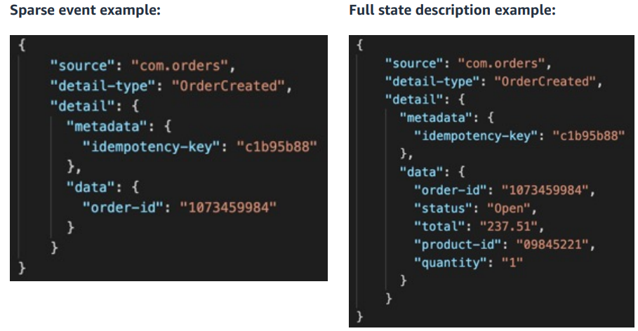
When starting on the journey to event-driven architectures, a common challenge is how to design events: “how much data should an event contain?” is a typical first question we encounter.
In this pragmatic post, you can explore the different types of events, watch a video that explains even further how to use event-driven architectures, and also go through the new event-driven architecture section of serverlessland.com.
Over the last few years, there has been a rise in the number of attacks that affect how a computer boots. Most modern computers use a specification called Unified Extensible Firmware Interface (UEFI) that defines a software interface between an operating system (e.g. Windows) and platform firmware (e.g. disk drives, video cards). There are security mechanisms built into UEFI that ensure that platform firmware can be cryptographically validated and boot securely through an application called a bootloader. This firmware is stored in non-volatile SPI flash memory on the motherboard, so it persists on the system even if the operating system is reinstalled and drives are replaced.
This creates a ‘trust anchor’ used to validate each stage of the boot process, but, unfortunately, this trust anchor is also a target for attack. In these UEFI attacks, malicious actions are loaded onto a compromised device early in the boot process. This means that malware can change configuration data, establish persistence by ‘implanting’ itself, and can bypass security measures that are only loaded at the operating system stage. So, while UEFI-anchored secure boot protects the bootloader from bootloader attacks, it does not protect the UEFI firmware itself.
Because of this growing trend of attacks, we began the process of cryptographically signing our UEFI firmware as a mitigation step. While our existing solution is platform specific to our x86 AMD server fleet, we did not have a similar solution to UEFI firmware signing for Arm. To determine what was missing, we had to take a deep dive into the Arm secure boot process.
Read on to learn about the world of Arm Trusted Firmware Secure Boot.
Arm Trusted Firmware Secure Boot
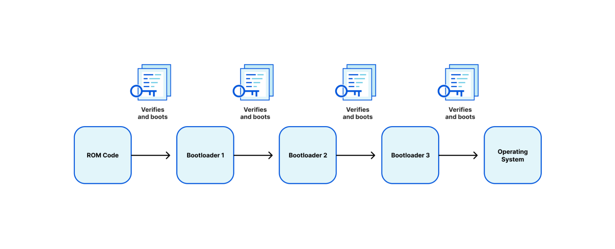
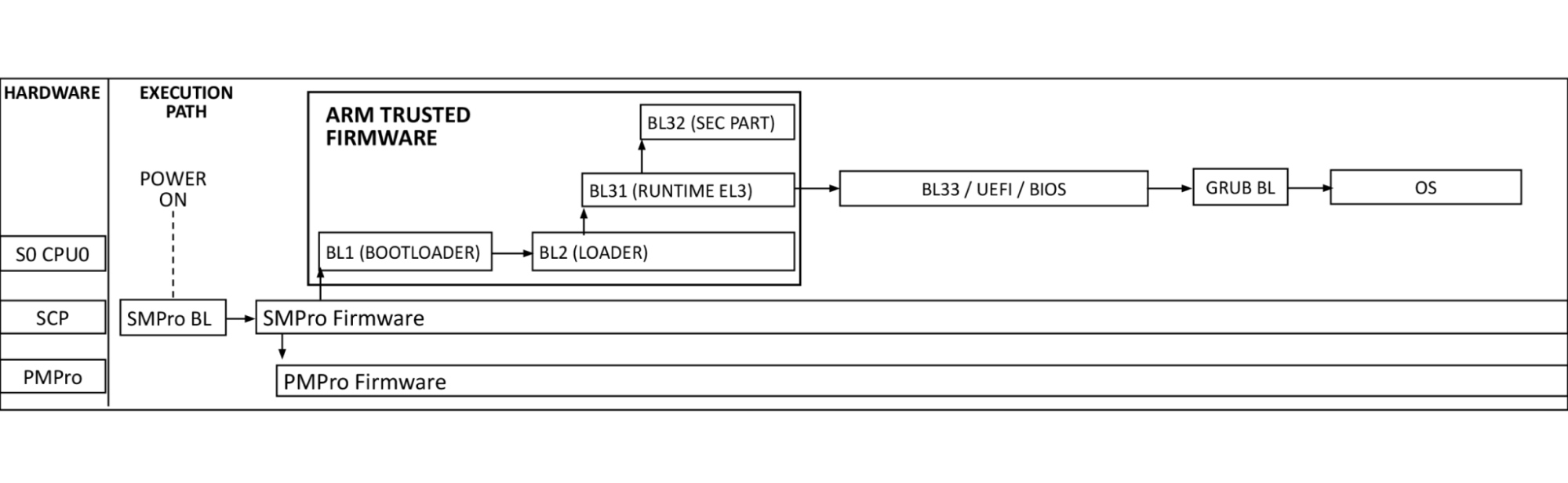
Arm defines a trusted boot process through an architecture called Trusted Board Boot Requirements (TBBR), or Arm Trusted Firmware (ATF) Secure Boot. TBBR works by authenticating a series of cryptographically signed binary images each containing a different stage or element in the system boot process to be loaded and executed. Every bootloader (BL) stage accomplishes a different stage in the initialization process:
BL1
BL1 defines the boot path (is this a cold boot or warm boot), initializes the architectures (exception vectors, CPU initialization, and control register setup), and initializes the platform (enables watchdog processes, MMU, and DDR initialization).
BL2
BL2 prepares initialization of the Arm Trusted Firmware (ATF), the stack responsible for setting up the secure boot process. After ATF setup, the console is initialized, memory is mapped for the MMU, and message buffers are set for the next bootloader.
BL3
The BL3 stage has multiple parts, the first being initialization of runtime services that are used in detecting system topology. After initialization, there is a handoff between the ATF ‘secure world’ boot stage to the ‘normal world’ boot stage that includes setup of UEFI firmware. Context is set up to ensure that no secure state information finds its way into the normal world execution state.
Each image is authenticated by a public key, which is stored in a signed certificate and can be traced back to a root key stored on the SoC in one time programmable (OTP) memory or ROM.
TBBR was originally designed for cell phones. This established a reference architecture on how to build a “Chain of Trust” from the first ROM executed (BL1) to the handoff to “normal world” firmware (BL3). While this creates a validated firmware signing chain, it has caveats:
SoC manufacturers are heavily involved in the secure boot chain, while the customer has little involvement.
A unique SoC SKU is required per customer. With one customer this could be easy, but most manufacturers have thousands of SKUs
The SoC manufacturer is primarily responsible for end-to-end signing and maintenance of the PKI chain. This adds complexity to the process requiring USB key fobs for signing.
Doesn’t scale outside the manufacturer.
What this tells us is what was built for cell phones doesn’t scale for servers.
If we were involved 100% in the manufacturing process, then this wouldn’t be as much of an issue, but we are a customer and consumer. As a customer, we have a lot of control of our server and block design, so we looked at design partners that would take some of the concepts we were able to implement with AMD Platform Secure Boot and refine them to fit Arm CPUs.
Amping it up
We partnered with Ampere and tested their Altra Max single socket rack server CPU (code named Mystique) that provides high performance with incredible power efficiency per core, much of what we were looking for in reducing power consumption. These are only a small subset of specs, but Ampere backported various features into the Altra Max notably, speculative attack mitigations that include Meltdown and Spectre (variants 1 and 2) from the Armv8.5 instruction set architecture, giving Altra the “+” designation in their ISA.
Ampere does implement a signed boot process similar to the ATF signing process mentioned above, but with some slight variations. We’ll explain it a bit to help set context for the modifications that we made.
Ampere Secure Boot
The diagram above shows the Arm processor boot sequence as implemented by Ampere. System Control Processors (SCP) are comprised of the System Management Processor (SMpro) and the Power Management Processor (PMpro). The SMpro is responsible for features such as secure boot and bmc communication while the PMpro is responsible for power features such as Dynamic Frequency Scaling and on-die thermal monitoring.
At power-on-reset, the SCP runs the system management bootloader from ROM and loads the SMpro firmware. After initialization, the SMpro spawns the power management stack on the PMpro and ATF threads. The ATF BL2 and BL31 bring up processor resources such as DRAM, and PCIe. After this, control is passed to BL33 BIOS.
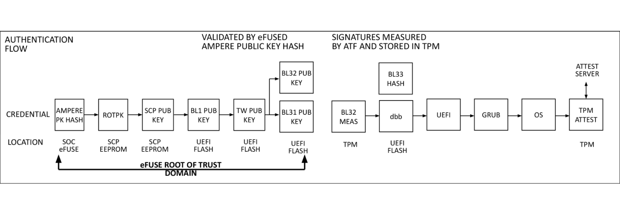
Authentication flow
At power on, the SMpro firmware reads Ampere’s public key (ROTPK) from the SMpro key certificate in SCP EEPROM, computes a hash and compares this to Ampere’s public key hash stored in eFuse. Once authenticated, Ampere’s public key is used to decrypt key and content certificates for SMpro, PMpro, and ATF firmware, which are launched in the order described above.
The SMpro public key will be used to authenticate the SMpro and PMpro images and ATF keys which in turn will authenticate ATF images. This cascading set of authentication that originates with the Ampere root key and stored in chip called an electronic fuse, or eFuse. An eFuse can be programmed only once, setting the content to be read-only and can not be tampered with nor modified.
This is the original hardware root of trust used for signing system, secure world firmware. When we looked at this, after referencing the signing process we had with AMD PSB and knowing there was a large enough one-time-programmable (OTP) region within the SoC, we thought: why can’t we insert our key hash in here?
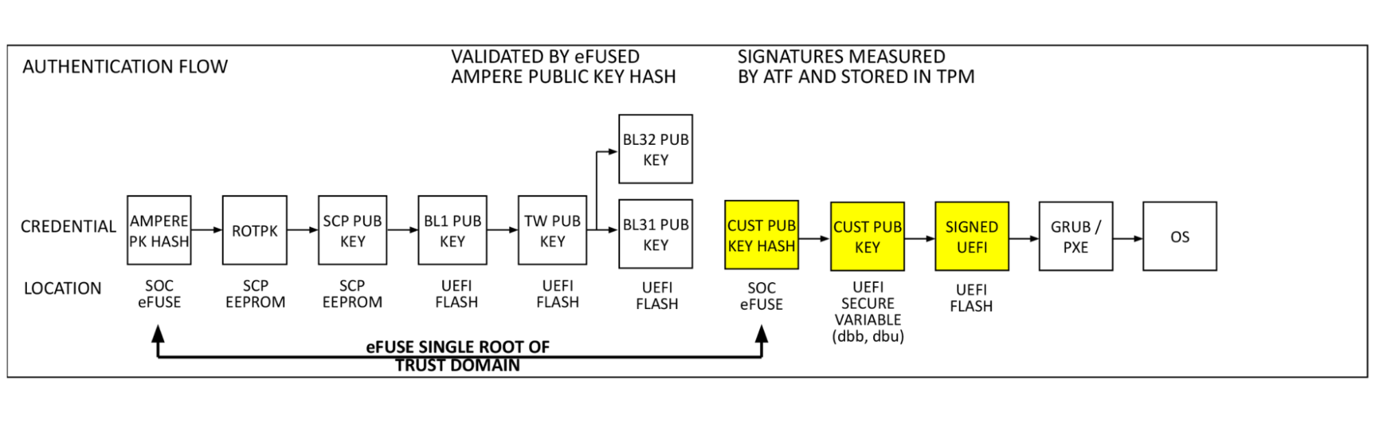
Single Domain Secure Boot
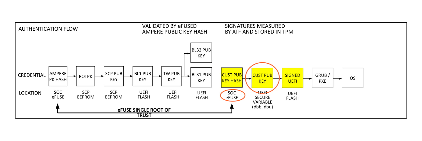
Single Domain Secure Boot takes the same authentication flow and adds a hash of the customer public key (Cloudflare firmware signing key in this case) to the eFuse domain. This enables the verification of UEFI firmware by a hardware root of trust. This process is performed in the already validated ATF firmware by BL2. Our public key (dbb) is read from UEFI secure variable storage, a hash is computed and compared to the public key hash stored in eFuse. If they match, the validated public key is used to decrypt the BL33 content certificate, validating and launching the BIOS, and remaining boot items. This is the key feature added by SDSB. It validates the entire software boot chain with a single eFuse root of trust on the processor.
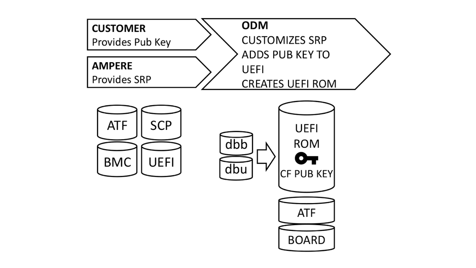
Building blocks
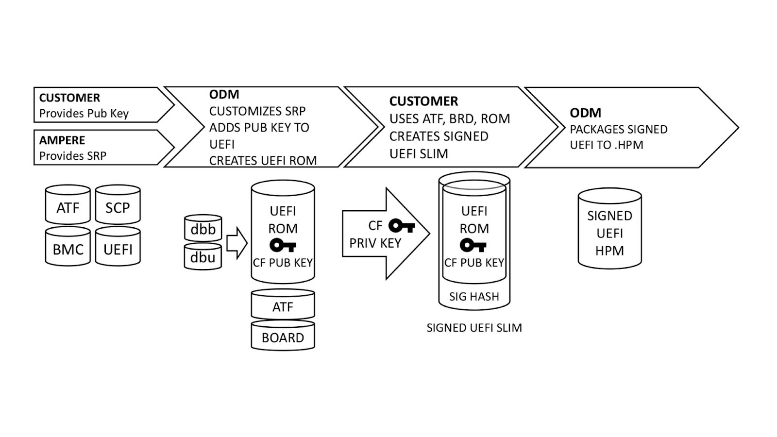
With a basic understanding of how Single Domain Secure Boot works, the next logical question is “How does it get implemented?”. We ensure that all UEFI firmware is signed at build time, but this process can be better understood if broken down into steps.
Ampere, our original device manufacturer (ODM), and we play a role in execution of SDSB. First, we generate certificates for a public-private key pair using our internal, secure PKI. The public key side is provided to the ODM as dbb.auth and dbu.auth in UEFI secure variable format. Ampere provides a reference Software Release Package (SRP) including the baseboard management controller, system control processor, UEFI, and complex programmable logic device (CPLD) firmware to the ODM, who customizes it for their platform. The ODM generates a board file describing the hardware configuration, and also customizes the UEFI to enroll dbb and dbu to secure variable storage on first boot.
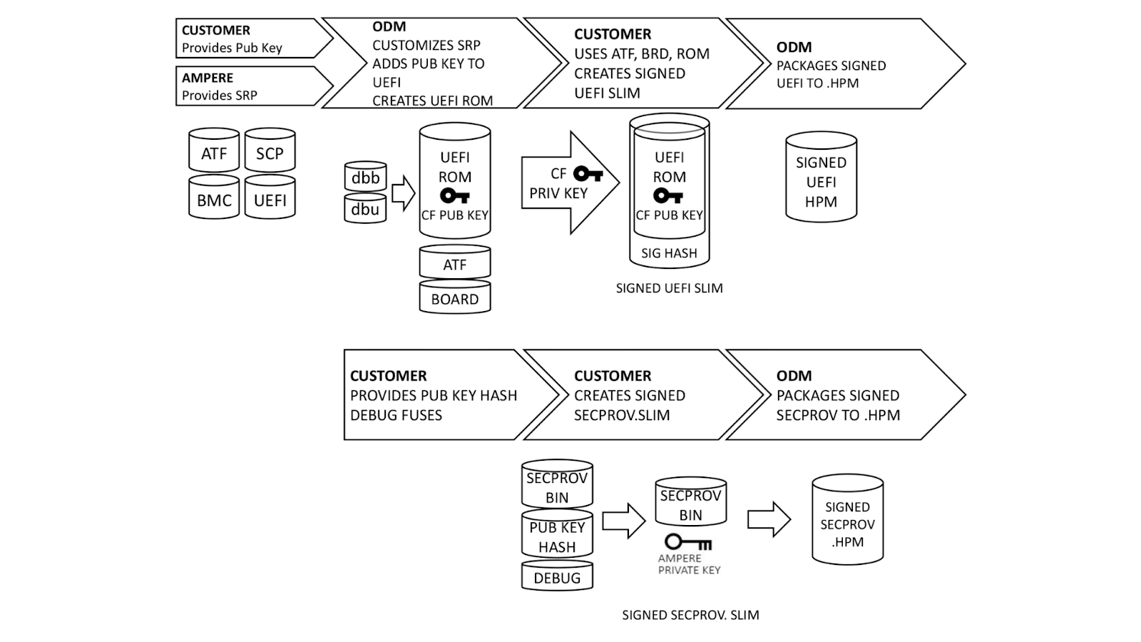
Once this is done, we generate a UEFI.slim file using the ODM’s UEFI ROM image, Arm Trusted Firmware (ATF) and Board File. (Note: This differs from AMD PSB insofar as the entire image and ATF files are signed; with AMD PSB, only the first block of boot code is signed.) The entire .SLIM file is signed with our private key, producing a signature hash in the file. This can only be authenticated by the correct public key. Finally, the ODM packages the UEFI into .HPM format compatible with their platform BMC.
In parallel, we provide the debug fuse selection and hash of our DER-formatted public key. Ampere uses this information to create a special version of the SCP firmware known as Security Provisioning (SECPROV) .slim format. This firmware is run one time only, to program the debug fuse settings and public key hash into the SoC eFuses. Ampere delivers the SECPROV .slim file to the ODM, who packages it into a .hpm file compatible with the BMC firmware update tooling.
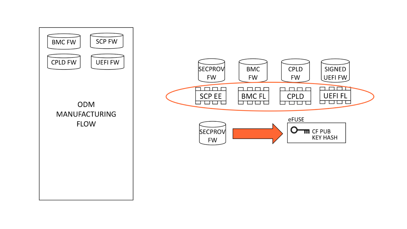
Fusing the keys
During system manufacturing, firmware is pre-programmed into storage ICs before placement on the motherboard. Note that the SCP EEPROM contains the SECPROV image, not standard SCP firmware. After a system is first powered on, an IPMI command is sent to the BMC which releases the Ampere processor from reset. This allows SECPROV firmware to run, burning the SoC eFuse with our public key hash and debug fuse settings.
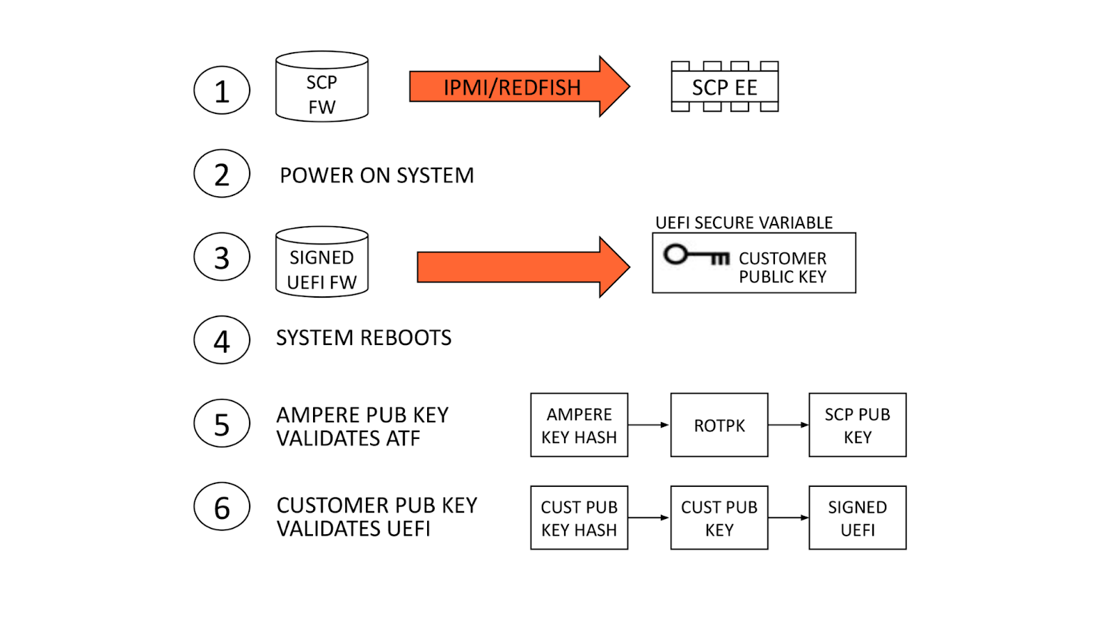
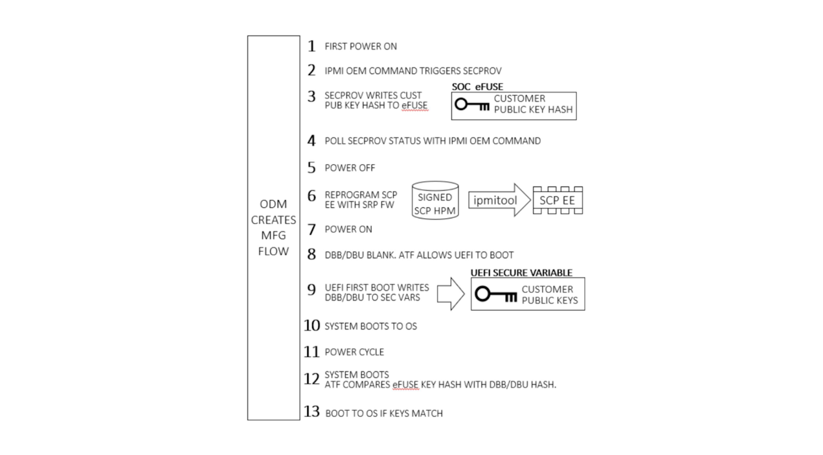
Final manufacturing flow
Once our public key has been provisioned, manufacturing proceeds by re-programming the SCP EEPROM with its regular firmware. Once the system powers on, ATF detects there are no keys present in secure variable storage and allows UEFI firmware to boot, regardless of signature. Since this is the first UEFI boot, it programs our public key into secure variable storage and reboots. ATF is validated by Ampere’s public key hash as usual. Since our public key is present in dbb, it is validated against our public key hash in eFuse and allows UEFI to boot.
Validation
The first part of validation requires observing successful destruction of the eFuses. This imprints our public key hash into a dedicated, immutable memory region, not allowing the hash to be overwritten. Upon automatic or manual issue of an IPMI OEM command to the BMC, the BMC observes a signal from the SECPROV firmware, denoting eFuse programming completion. This can be probed with BMC commands.
When the eFuses have been blown, validation continues by observing the boot chain of the other firmware. Corruption of the SCP, ATF, or UEFI firmware obstructs boot flow and boot authentication and will cause the machine to fail booting to the OS. Once firmware is in place, happy path validation begins with booting the machine.
Upon first boot, firmware boots in the following order: BMC, SCP, ATF, and UEFI. The BMC, SCP, and ATF firmware can be observed via their respective serial consoles. The UEFI will automatically enroll the dbb and dbu files to the secure variable storage and trigger a reset of the system.
After observing the reset, the machine should successfully boot to the OS if the feature is executed correctly. For further validation, we can use the UEFI shell environment to extract the dbb file and compare the hash against the hash submitted to Ampere. After successfully validating the keys, we flash an unsigned UEFI image. An unsigned UEFI image causes authentication failure at bootloader stage BL3-2. The ATF firmware undergoes a boot loop as a result. Similar results will occur for a UEFI image signed with incorrect keys.
Updated authentication flow
On all subsequent boot cycles, the ATF will read secure variable dbb (our public key), compute a hash of the key, and compare it to the read-only Cloudflare public key hash in eFuse. If the computed and eFuse hashes match, our public key variable can be trusted and is used to authenticate the signed UEFI. After this, the system boots to the OS.
Let’s boot!
We were unable to get a machine without the feature enabled to demonstrate the set-up of the feature since we have the eFuse set at build time, but we can demonstrate what it looks like to go between an unsigned BIOS and a signed BIOS. What we would have observed with the set-up of the feature is a custom BMC command to instruct the SCP to burn the ROTPK into the SOC’s OTP fuses. From there, we would observe feedback to the BMC detailing whether burning the fuses was successful. Upon booting the UEFI image for the first time, the UEFI will write the dbb and dbu into secure storage.
As you can see, after flashing the unsigned BIOS, the machine fails to boot.
Despite the lack of visibility in failure to boot, there are a few things going on underneath the hood. The SCP (System Control Processor) still boots.
The SCP image holds a key certificate with Ampere’s generated ROTPK and the SCP key hash. SCP will calculate the ROTPK hash and compare it against the burned OTP fuses. In the failure case, where the hash does not match, you will observe a failure as you saw earlier. If successful, the SCP firmware will proceed to boot the PMpro and SMpro. Both the PMpro and SMpro firmware will be verified and proceed with the ATF authentication flow.
The conclusion of the SCP authentication is the passing of the BL1 key to the first stage bootloader via the SCP HOB(hand-off-block) to proceed with the standard three stage bootloader ATF authentication mentioned previously.
At BL2, the dbb is read out of the secure variable storage and used to authenticate the BL33 certificate and complete the boot process by booting the BL33 UEFI image.
Still more to do
In recent years, management interfaces on servers, like the BMC, have been the target of cyber attacks including ransomware, implants, and disruptive operations. Access to the BMC can be local or remote. With remote vectors open, there is potential for malware to be installed on the BMC via network interfaces. With compromised software on the BMC, malware or spyware could maintain persistence on the server. An attacker might be able to update the BMC directly using flashing tools such as flashrom or socflash without the same level of firmware resilience established at the UEFI level.
The future state involves using host CPU-agnostic infrastructure to enable a cryptographically secure host prior to boot time. We will look to incorporate a modular approach that has been proposed by the Open Compute Project’s Data Center Secure Control
Module Specification (DC-SCM) 2.0 specification. This will allow us to standardize our Root of Trust, sign our BMC, and assign physically unclonable function (PUF) based identity keys to components and peripherals to limit the use of OTP fusing. OTP fusing creates a problem with trying to “e-cycle” or reuse machines as you cannot truly remove a machine identity.
In our first seminar of 2023, we were delighted to welcome Dr Katie Rich and Carla Strickland. They spoke to us about teaching the programming construct of variables in Grade 3 and 4 (age 8 to 10).
Dr Katie RichCarla Strickland
We are hearing from a diverse range of speakers in our current series of monthly online research seminars focused on primary (K-5) computing education. Many of them work closely with educators to translate research findings into classroom practice to make sure that all our younger learners have positive first experiences of learning computing. An important goal of their research is to impact the development of pedagogy, resources, and professional development to support educators to deliver computing concepts with confidence.
Variables in computing and mathematics
Dr Katie Rich (American Institutes of Research) and Carla Strickland (UChicago STEM Education) are both part of a team that worked on a research project called Everyday Computing, which aims to integrate computational thinking into primary mathematics lessons. A key part of the Everyday Computing project was to develop coherent learning resources across a number of school years. During the seminar, Katie and Carla presented on a study in the project that revolved around teaching variables in Grade 3 and 4 (age 8 to 10) by linking this computing concept to mathematical concepts such as area, perimeter, and fractions.
Variables are used in both mathematics and computing, but in significantly different ways. In mathematics, a variable, often represented by a single letter such as x or y, corresponds to a quantity that stays the same for a given problem. However, in computing, a variable is an identifier used to label data that may change as a computer program is executed. A variable is one of the programming constructs that can be used to generalise programs to make them work for a range of inputs. Katie highlighted that the research team was keen to explore the synergies and tensions that arise when curriculum subjects share terms, as is the case for ‘variable’.
Defining a learning trajectory
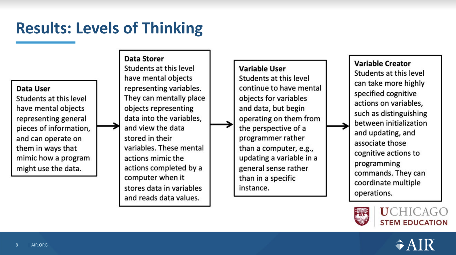
At the start of the project, in order to be able to develop coherent learning resources across school years, the team reviewed research papers related to teaching the programming construct of variables. In the papers, they found a variety of learning goals that related to facts (what learners need to know) and skills (what learners need to be able to do). They grouped these learning goals and arranged the groups into ‘levels of thinking’, which were then mapped onto a learning trajectory to show progression pathways for learning.
Four of the five levels of thinking identified in the study: Data Storer, Data User, Variable User, Variable Creator. Click to enlarge.
Learning materials about variables
Carla then shared three practical examples of learning resources their research team created that integrated the programming construct of variables into a maths curriculum. The three activities, described below, form part of a series of lessons called Action Fractions. You can read more about the series of lessons in this research paper.
Robot Boxesis an unpluggedactivity that is positioned at the Data User level of thinking. It relates to creating instructions for a fictional robot. Learners have to pay attention to different data the robot needs in order to draw a box, such as the length and width, and also to the value that the robot calculates as area of the box. The lesson uses boxes on paper as concrete representations of variables to which learners can physically add values.
Ambling Animals is set at the ‘Data Storer’ and ‘Variable Interpreter’ levels of thinking. It includes a Scratch project to help students to locate and compare fractions on number lines. During this lesson, find a variable that holds the value of the animal that represents the larger of two fractions.
Adding Fractions draws on facts and skills from the ‘Variable Interpreter’ and ‘Variable Implementer’ levels of thinking and also includes a Scratch project. The Scratch project visualises adding fractions with the same denominator on a number line. The lesson starts to explain why variables are so important in computer programs by demonstrating how using a variable can make code more efficient.
Takeaways: Cross-curricular teaching, collaborative research
Teaching about the programming construct of variables can be challenging, as it requires young learners to understand abstract ideas. The research Katie and Carla presented shows how integrating these concepts into a mathematics curriculum is one way to highlight tangible uses of variables in everyday problems. The levels of thinking in the learning trajectory provide a structure helping teachers to support learners to develop their understanding and skills; the same levels of thinking could be used to introduce variables in other contexts and curricula.
Many primary teachers use cross-curricular learning to increase children’s engagement and highlight real-world examples. The seminar showed how important it is for teachers to pay attention to terms used across subjects, such as the word ‘variable’, and to explicitly explain a term’s different meanings. Katie and Carla shared a practical example of this when they suggested that computing teachers need to do more to stress the difference between equations such as xy = 45 in maths and assignment statements such as length = 45 in computing.
The Everyday Computing project resources were created by a team of researchers and educators who worked together to translate research findings into curriculum materials. This type of collaboration can be really valuable in driving a research agenda to directly improve learning outcomes for young people in classrooms.
How can this research influence your classroom practice or other activities as an educator? Let us know your thoughts in the comments. We’ll be continuing to reflect on this question throughout the seminar series.
You can watch Katie’s and Carla’s full presentation here:
Join our seminar series on primary computing education
We continue on Tuesday 7 February at 17.00 UK time, when we will hear from Dr Jean Salac, University of Washington. Jean will present her work in identifying inequities in elementary computing instruction and in developing a learning strategy, TIPP&SEE, to address these inequities. Sign up now, and we will send you a joining link for the session.
The head of both US Cyber Command and the NSA, Gen. Paul Nakasone, broadly discussed that first organization’s offensive cyber operations during the runup to the 2022 midterm elections. He didn’t name names, of course:
We did conduct operations persistently to make sure that our foreign adversaries couldn’t utilize infrastructure to impact us,” said Nakasone. “We understood how foreign adversaries utilize infrastructure throughout the world. We had that mapped pretty well. And we wanted to make sure that we took it down at key times.”
Nakasone noted that Cybercom’s national mission force, aided by NSA, followed a “campaign plan” to deprive the hackers of their tools and networks. “Rest assured,” he said. “We were doing operations well before the midterms began, and we were doing operations likely on the day of the midterms.” And they continued until the elections were certified, he said.
We know Cybercom did similar things in 2018 and 2020, and presumably will again in two years.
Several Cloudflare services became unavailable for 121 minutes on January 24th, 2023 due to an error releasing code that manages service tokens. The incident degraded a wide range of Cloudflare products including aspects of our Workers platform, our Zero Trust solution, and control plane functions in our content delivery network (CDN).
Cloudflare provides a service token functionality to allow automated services to authenticate to other services. Customers can use service tokens to secure the interaction between an application running in a data center and a resource in a public cloud provider, for example. As part of the release, we intended to introduce a feature that showed administrators the time that a token was last used, giving users the ability to safely clean up unused tokens. The change inadvertently overwrote other metadata about the service tokens and rendered the tokens of impacted accounts invalid for the duration of the incident.
The reason a single release caused so much damage is because Cloudflare runs on Cloudflare. Service tokens impact the ability for accounts to authenticate, and two of the impacted accounts power multiple Cloudflare services. When these accounts’ service tokens were overwritten, the services that run on these accounts began to experience failed requests and other unexpected errors.
We know this impacted several customers and we know the impact was painful. We’re documenting what went wrong so that you can understand why this happened and the steps we are taking to prevent this from occurring again.
What is a service token?
When users log into an application or identity provider, they typically input a username and a password. The password allows that user to demonstrate that they are in control of the username and that the service should allow them to proceed. Layers of additional authentication can be added, like hard keys or device posture, but the workflow consists of a human proving they are who they say they are to a service.
However, humans are not the only users that need to authenticate to a service. Applications frequently need to talk to other applications. For example, imagine you build an application that shows a user information about their upcoming travel plans.
The airline holds details about the flight and its duration in their own system. They do not want to make the details of every individual trip public on the Internet and they do not want to invite your application into their private network. Likewise, the hotel wants to make sure that they only send details of a room booking to a valid, approved third party service.
Your application needs a trusted way to authenticate with those external systems. Service tokens solve this problem by functioning as a kind of username and password for your service. Like usernames and passwords, service tokens come in two parts: a Client ID and a Client Secret. Both the ID and Secret must be sent with a request for authentication. Tokens are also assigned a duration, after which they become invalid and must be rotated. You can grant your application a service token and, if the upstream systems you need validate it, your service can grab airline and hotel information and present it to the end user in a joint report.
When administrators create Cloudflare service tokens, we generate the Client ID and the Client Secret pair. Customers can then configure their requesting services to send both values as HTTP headers when they need to reach a protected resource. The requesting service can run in any environment, including inside of Cloudflare’s network in the form of a Worker or in a separate location like a public cloud provider. Customers need to deploy the corresponding protected resource behind Cloudflare’s reverse proxy. Our network checks every request bound for a configured service for the HTTP headers. If present, Cloudflare validates their authenticity and either blocks the request or allows it to proceed. We also log the authentication event.
Incident Timeline
All Timestamps are UTC
At 2023-01-24 16:55 UTC the Access engineering team initiated the release that inadvertently began to overwrite service token metadata, causing the incident.
At 2023-01-24 17:05 UTC a member of the Access engineering team noticed an unrelated issue and rolled back the release which stopped any further overwrites of service token metadata.
Service token values are not updated across Cloudflare’s network until the service token itself is updated (more details below). This caused a staggered impact of the service token’s that had their metadata overwritten.
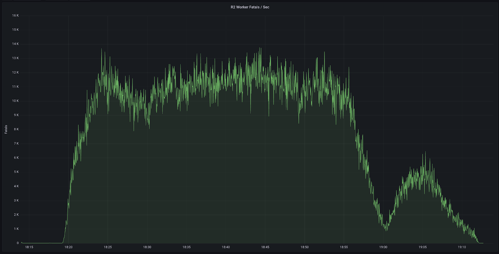
2023-01-24 17:50 UTC: The first invalid service token for Cloudflare WARP was synced to the edge. Impact began for WARP and Zero Trust users.
WARP device posture uploads dropped to zero which raised an internal alert
At 2023-01-24 18:12 an incident was declared due to the large drop in successful WARP device posture uploads.
2023-01-24 18:19 UTC: The first invalid service token for the Cloudflare API was synced to the edge. Impact began for Cache Purge, Cache Reserve, Images and R2. Alerts were triggered for these products which identified a larger scope of the incident.
At 2023-01-24 18:21 the overwritten services tokens were discovered during the initial investigation.
At 2023-01-24 18:28 the incident was elevated to include all impacted products.
At 2023-01-24 18:51 An initial solution was identified and implemented to revert the service token to its original value for the Cloudflare WARP account, impacting WARP and Zero Trust. Impact ended for WARP and Zero Trust.
At 2023-01-24 18:56 The same solution was implemented on the Cloudflare API account, impacting Cache Purge, Cache Reserve, Images and R2. Impact ended for Cache Purge, Cache Reserve, Images and R2.
At 2023-01-24 19:00 An update was made to the Cloudflare API account which incorrectly overwrote the Cloudflare API account. Impact restarted for Cache Purge, Cache Reserve, Images and R2. All internal Cloudflare account changes were then locked until incident resolution.
At 2023-01-24 19:07 the Cloudflare API was updated to include the correct service token value. Impact ended for Cache Purge, Cache Reserve, Images and R2.
At 2023-01-24 19:51 all affected accounts had their service tokens restored from a database backup. Incident Ends.
What was released and how did it break?
The Access team was rolling out a new change to service tokens that added a “Last seen at” field. This was a popular feature request to help identify which service tokens were actively in use.
What went wrong?
The “last seen at” value was derived by scanning all new login events in an account’s login event Kafka queue. If a login event using a service token was detected, an update to the corresponding service token’s last seen value was initiated.
In order to update the service token’s “last seen at” value a read write transaction is made to collect the information about the corresponding service token. Service token read requests redact the “client secret” value by default for security reasons. The “last seen at” update to the service token then used that information from the read did not include the “client secret” and updated the service token with an empty “client secret” on the write.
An example of the correct and incorrect service token values shown below:
Example Access Service Token values
{
  "1a4ddc9e-a1234-4acc-a623-7e775e579c87": {
    "client_id": "6b12308372690a99277e970a3039343c.access",
    "client_secret": "<hashed-value>", <-- what you would expect
    "expires_at": 1698331351
  },
  "23ade6c6-a123-4747-818a-cd7c20c83d15": {
    "client_id": "1ab44976dbbbdadc6d3e16453c096b00.access",
    "client_secret": "", <--- this is the problem
    "expires_at": 1670621577
  }
}
The service token “client secret” database did have a “not null” check however in this situation an empty text string did not trigger as a null value.
As a result of the bug, any Cloudflare account that used a service token to authenticate during the 10 minutes “last seen at” release was out would have its “client secret” value set to an empty string. The service token then needed to be modified in order for the empty “client secret” to be used for authentication. There were a total of 4 accounts in this state, all of which are internal to Cloudflare.
How did we fix the issue?
As a temporary solution, we were able to manually restore the correct service token values for the accounts with overwritten service tokens. This stopped the immediate impact across the affected Cloudflare services.
The database team was then able to implement a solution to restore the service tokens of all impacted accounts from an older database copy. This concluded any impact from this incident.
Why did this impact other Cloudflare services?
Service tokens impact the ability for accounts to authenticate. Two of the impacted accounts power multiple Cloudflare services. When these accounts’ services tokens were overwritten, the services that run on these accounts began to experience failed requests and other unexpected errors.
Cloudflare WARP Enrollment
Cloudflare provides a mobile and desktop forward proxy, Cloudflare WARP (our “1.1.1.1” app), that any user can install on a device to improve the privacy of their Internet traffic. Any individual can install this service without the need for a Cloudflare account and we do not retain logs that map activity to a user.
When a user connects using WARP, Cloudflare validates the enrollment of a device by relying on a service that receives and validates the keys on the device. In turn, that service communicates with another system that tells our network to provide the newly enrolled device with access to our network
During the incident, the enrollment service could no longer communicate with systems in our network that would validate the device. As a result, users could no longer register new devices and/or install the app on a new device, and may have experienced issues upgrading to a new version of the app (which also triggers re-registration).
Cloudflare Zero Trust Device Posture and Re-Auth Policies
Cloudflare provides a comprehensive Zero Trust solution that customers can deploy with or without an agent living on the device. Some use cases are only available when using the Cloudflare agent on the device. The agent is an enterprise version of the same Cloudflare WARP solution and experienced similar degradation anytime the agent needed to send or receive device state. This impacted three use cases in Cloudflare Zero Trust.
First, similar to the consumer product, new devices could not be enrolled and existing devices could not be revoked. Administrators were also unable to modify settings of enrolled devices.. In all cases errors would have been presented to the user.
Second, many customers who replace their existing private network with Cloudflare’s Zero Trust solution may add rules that continually validate a user’s identity through the use of session duration policies. The goal of these rules is to enforce users to reauthenticate in order to prevent stale sessions from having ongoing access to internal systems. The agent on the device prompts the user to reauthenticate based on signals from Cloudflare’s control plane. During the incident, the signals were not sent and users could not successfully reauthenticate.
Finally, customers who rely on device posture rules also experienced impact. Device posture rules allow customers who use Access or Gateway policies to rely on the WARP agent to continually enforce that a device meets corporate compliance rules.
The agent communicates these signals to a Cloudflare service responsible for maintaining the state of the device. Cloudflare’s Zero Trust access control product uses a service token to receive this signal and evaluate it along with other rules to determine if a user can access a given resource. During this incident those rules defaulted to a block action, meaning that traffic modified by these policies would appear broken to the user. In some cases this meant that all internet bound traffic from a device was completely blocked leaving users unable to access anything.
Cloudflare Gateway caches the device posture state for users every 5 minutes to apply Gateway policies. The device posture state is cached so Gateway can apply policies without having to verify device state on every request. Depending on which Gateway policy type was matched, the user would experience two different outcomes. If they matched a network policy the user would experience a dropped connection and for an HTTP policy they would see a 5XX error page. We peaked at over 50,000 5XX errors/minute over baseline and had over 10.5 million posture read errors until the incident was resolved.
Gateway 5XX errors per minute
Total count of Gateway Device posture errors
Cloudflare R2 Storage and Cache Reserve
Cloudflare R2 Storage allows developers to store large amounts of unstructured data without the costly egress bandwidth fees associated with typical cloud storage services.
During the incident, the R2 service was unable to make outbound API requests to other parts of the Cloudflare infrastructure. As a result, R2 users saw elevated request failure rates when making requests to R2.
Many Cloudflare products also depend on R2 for data storage and were also affected. For example, Cache Reserve users were impacted during this window and saw increased origin load for any items not in the primary cache. The majority of read and write operations to the Cache Reserve service were impacted during this incident causing entries into and out of Cache Reserve to fail. However, when Cache Reserve sees an R2 error, it falls back to the customer origin, so user traffic was still serviced during this period.
Cloudflare Cache Purge
Cloudflare’s content delivery network (CDN) caches the content of Internet properties on our network in our data centers around the world to reduce the distance that a user’s request needs to travel for a response. In some cases, customers want to purge what we cache and replace it with different data.
The Cloudflare control plane, the place where an administrator interacts with our network, uses a service token to authenticate and reach the cache purge service. During the incident, many purge requests failed while the service token was invalid. We saw an average impact of 20 purge requests/second failing and a maximum of 70 requests/second.
What are we doing to prevent this from happening again?
We take incidents like this seriously and recognize the impact it had. We have identified several steps we can take to address the risk of a similar problem occurring in the future. We are implementing the following remediation plan as a result of this incident:
Test: The Access engineering team will add unit tests that would automatically catch any similar issues with service token overwrites before any new features are launched.
Alert: The Access team will implement an automatic alert for any dramatic increase in failed service token authentication requests to catch issues before they are fully launched.
Process: The Access team has identified process improvements to allow for faster rollbacks for specific database tables.
Implementation: All relevant database fields will be updated to include checks for empty strings on top of existing “not null checks”
We are sorry for the disruption this caused for our customers across a number of Cloudflare services. We are actively making these improvements to ensure improved stability moving forward and that this problem will not happen again.
The Python community is currently struggling with a longtime difficulty in
its ecosystem: how to develop, package, distribute, and maintain libraries
and applications. The current situation is sub-optimal in several
dimensions due, at least in part, to the existence of multiple,
non-interoperable mechanisms and tools to handle some of those needs. Last
week, we had an overview of Python
packaging as a prelude to starting to dig into the discussions. In
this installment, we start to look at the kinds of problems that exist—and
the barriers to solving them.
The collective thoughts of the interwebz
Manage Consent
To provide the best experiences, we use technologies like cookies to store and/or access device information. Consenting to these technologies will allow us to process data such as browsing behavior or unique IDs on this site. Not consenting or withdrawing consent, may adversely affect certain features and functions.
Functional
Always active
The technical storage or access is strictly necessary for the legitimate purpose of enabling the use of a specific service explicitly requested by the subscriber or user, or for the sole purpose of carrying out the transmission of a communication over an electronic communications network.
Preferences
The technical storage or access is necessary for the legitimate purpose of storing preferences that are not requested by the subscriber or user.
Statistics
The technical storage or access that is used exclusively for statistical purposes.The technical storage or access that is used exclusively for anonymous statistical purposes. Without a subpoena, voluntary compliance on the part of your Internet Service Provider, or additional records from a third party, information stored or retrieved for this purpose alone cannot usually be used to identify you.
Marketing
The technical storage or access is required to create user profiles to send advertising, or to track the user on a website or across several websites for similar marketing purposes.