Tag Archives: Amazon EMR

How Ancestry optimizes a 100-billion-row Iceberg table

Post Syndicated from Thomas Cardenas original https://aws.amazon.com/blogs/big-data/how-ancestry-optimizes-a-100-billion-row-iceberg-table/

This is a guest post by Thomas Cardenas, Staff Software Engineer at Ancestry, in partnership with AWS.

Ancestry, the global leader in family history and consumer genomics, uses family trees, historical records, and DNA to help people on their journeys of personal discovery. Ancestry has the largest collection of family history records, consisting of 40 billion records. They serve more than 3 million subscribers and have over 23 million people in their growing DNA network. Their customers can use this data to discover their family story.

Ancestry is proud to connect users with their families past and present. They help people learn more about their own identity by learning about their ancestors. Users build a family tree through which we surface relevant records, historical documents, photos, and stories that might contain details about their ancestors. These artifacts are surfaced through Hints. The Hints dataset is one of the most interesting datasets at Ancestry. It’s used to alert users that potential new information is available. The dataset has multiple shards, and there are currently 100 billion rows being used by machine learning models and analysts. Not only is the dataset large, it also changes rapidly.

In this post, we share the best practices that Ancestry used to implement an Apache Iceberg-based hints table capable of handling 100 billion rows with 7 million hourly changes. The optimizations covered here resulted in cost reductions of 75%.

Overview of solution

Ancestry’s Enterprise Data Management (EDM) team faced a critical challenge—how to provide a unified, performant data ecosystem that could serve diverse analytical workloads across financial, marketing, and product analytics teams. The ecosystem needed to support everything from data scientists training recommendation models to geneticists developing population studies—all requiring access to the same Hints data.

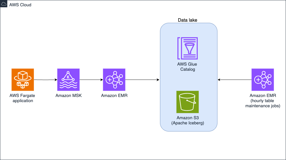
The ecosystem around Hints data had been developed organically, without a well-defined architecture. Teams independently accessed Hints data through direct service calls, Kafka topic subscriptions, or warehouse queries, creating significant data duplication and unnecessary system load. To reduce cost and improve performance, EDM implemented a centralized Apache Iceberg data lake on Amazon Simple Storage Service (Amazon S3), with Amazon EMR providing the processing power. This architecture, shown in the following image, creates a single source of truth for the Hints dataset while using Iceberg’s ACID transactions, schema evolution, and partition evolution capabilities to handle scale and update frequency.

End-to-end AWS analytics architecture showcasing data movement from Fargate through MSK, EMR, to S3 data lake with Glue Catalog

Hints table management architecture

Managing datasets exceeding one billion rows presents unique challenges, and Ancestry faced this challenge with the trees collection of 20–100 billion rows across multiple tables. At this scale, dataset updates require careful execution to control costs and prevent memory issues. To solve these challenges, EDM chose Amazon EMR on Amazon EC2 running Spark to write Iceberg tables on Amazon S3 for storage. With large and steady Amazon EMR workloads, running the clusters on Amazon EC2, as opposed to Serverless, proved cost effective. EDM has scheduled an Apache Spark job to run every hour on their Amazon EMR on EC2. This job uses the merge operation to update the Iceberg table with recently changed rows. Performing updates like this on such a large dataset can easily lead to runaway costs and out-of-memory errors.

Key optimization techniques

The engineers needed to enable fast, row-level updates without impacting query performance or incurring substantial cost. To achieve this, Ancestry used a combination of partitioning strategies, table configurations, Iceberg procedures, and incremental updates. The following is covered in detail:

  • Partitioning
  • Sorting
  • Merge-on-read
  • Compaction
  • Snapshot management
  • Storage-partitioned joins

Partitioning strategy

Developing an effective partitioning strategy was crucial for the 100-billion-row Hints table. Iceberg supports various partition transforms including column value, temporal functions (year, month, day, hour), and numerical transforms (bucket, truncate). Following AWS best practices, Ancestry carefully analyzed query patterns to identify a partitioning approach that would support these queries while balancing these two competing considerations:

  • Too few partitions would force queries to scan excessive data, degrading performance and increasing costs.
  • Too many partitions would create small files and excessive metadata, causing management overhead and slower query planning. It’s generally best to avoid parquet files smaller than 100 MB.

Through query pattern analysis, Ancestry discovered that most analytical queries filtered on hint status (particularly pending status) and hint type. This insight led us to implement a two-level partitioning strategy-first on status and then on type, which dramatically reduced the amount of data scanned during typical queries.

Sorting

To further optimize query performance, Ancestry implemented strategic data organization within partitions using Iceberg’s sort orders. While Iceberg doesn’t maintain perfect ordering, even approximate sorting significantly improves data locality and compression ratios.

For the Hints table with 100 billion rows, Ancestry faced a unique challenge: the primary identifiers (PersonId and HintId) are high-cardinality numeric columns that would be prohibitively expensive to sort completely. The solution uses Iceberg’s truncate transform function to support sorting on just a portion of the number, effectively creating another partition by grouping a collection of IDs together. For example, we can specify truncate(100_000_000, hintId) to create groups of 100 million hint IDs, greatly improving the performance of queries that specify that column.

Merge on read

With 7 million changes to the Hints table occurring hourly, optimizing write performance became critical to the architecture. In addition to making sure queries performed well, Ancestry also needed to make sure our frequent updates would perform well in both time and cost. It was quickly discovered that the default copy-on-write (CoW) strategy, which copies an entire file when any part of it changes, was too slow and expensive for their use case. Ancestry was able to get the performance we needed by instead specifying the merge-on-read (MoR) update strategy, which maintains new information in diff files that are reconciled on read. The large updates that happen every hour led us to choose faster updates at the cost of slower reads.

File compaction

The frequent updates mean files are constantly needing to be re-written to maintain performance. Iceberg provides the rewrite_data_files procedure for compaction, but default configurations proved insufficient for our scale. Leaving the default configuration in place, the rewrite operation wrote to five partitions at a time and didn’t meet our performance objective. We found that increasing the concurrent writes improved performance. We used the following set of parameters, setting a relatively high max-concurrent-file-group-rewrites value of 100 to more efficiently deal with our thousands of partitions. The default of rewriting only one file at a time couldn’t keep up with the frequency of our updates.

CALL datalake.system.rewrite_data_files(
  table => ‘database.table’, 
  strategy => ‘binpack’, 
  options => map (
    'max-concurrent-file-group-rewrites','100',
    'partial-progress.enabled','true',
    'rewrite-all','true'
  )
)

Key optimizations in Ancestry’s approach include:

  • High concurrency: We increased max-concurrent-file-group-rewrites from the default 5 to 100, enabling parallel processing of our thousands of partitions. This increased compute costs but was necessary to help ensure that the jobs finished.
  • Resilience at scale: We enabled partial-progress to create compaction checkpoints, essential when operating at our scale where failures are particularly costly.
  • Comprehensive delta elimination: Setting rewrite-all to true helps ensure that both data files and delete files are compacted, preventing the accumulation of delete files. By default, the delete files created as part of this strategy aren’t re-written and would continue to accumulate, slowing queries.

We arrived at these optimizations through successive trials and evaluations. For example, with our very large dataset, we discovered that we could use a WHERE clause to limit re-writes to a single partition. Based on the partitions, we see varied execution times and resource utilization. For some partitions, we needed to reduce concurrency to avoid running into out of memory errors.

Snapshot management

Iceberg tables maintain snapshots to preserve the history of the table, allowing you to time travel through the changes. As these snapshots accrue, they add to storage costs and degrade performance. This is why maintaining an Iceberg table requires you to periodically call the expire_snapshots procedure. We found we needed to enable concurrency for snapshot management so that it would complete in a timely manner:

CALL datalake.system.expire_snapshots(
        table => '`database`.table', 
        retain_last => 1, 
        max_concurrent_deletes => 20)

Consider how to balance performance, cost, and the need to keep historical records depending on your use case. When you do so, note that there is a table-level setting for maximum snapshot age which can override the retain_last parameter and retain only the active snapshot.

Reducing shuffle with Storage-Partitioned Joins

We use Storage-Partitioned Joins (SPJ) in Iceberg tables to minimize expensive shuffles during data processing. SPJ is an advanced Iceberg feature (available in Spark 3.3 or later with Iceberg 1.2 or later) that uses the physical storage layout of tables to eliminate shuffle operations entirely. For our Hints update pipeline, this optimization was transformational.

SPJ is especially useful during MERGE INTO operations, where datasets have identical partitioning. Proper configuration helps ensure effective use of SPJ to optimize joins.

SPJ has a few requirements such as both tables must be Iceberg partitioned the same way and joined on the partition key. Then Iceberg will know that it doesn’t have to shuffle the data when the tables are loaded. This even works when there are a different number of partitions on either side.

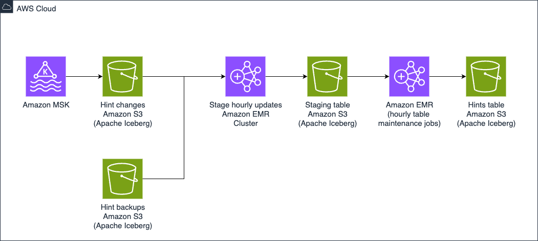
Updates to the Hints database are first staged in the Hint Changes database where data is transformed from the original Kafka data format into how it will look in the target (Hints) table. This is a temporary Iceberg table where we are able to perform audits using Write-Audit-Publish (WAP) pattern. In addition to using the WAP pattern we are able to use the SPJ functionality.

Technical workflow showing AWS data processing pipeline with following sequence: Amazon MSK starting point Parallel paths to: Hint changes in S3 (Apache Iceberg) Hint backups in S3 (Apache Iceberg) Stage hourly updates via EMR Cluster Staging table in S3 (Apache Iceberg) EMR hourly table maintenance jobs Final hints table in S3 (Apache Iceberg)

The Hints data pipeline

Reducing full-table scans

Another strategy to reduce shuffle is minimizing the data involved in joins by dynamically pushing down filters. In production, these filters vary between batches, so a multi-step operation is often necessary for setting up merges. The following example code first limits its scope by setting minimum and maximum values for the ID, then performs an update or delete to the target table depending on whether a target value exists.

val stats: Dataset[Row] = session.read.table("catalog.database.source")
  .agg(
    min(col("id")).as("min_value"),
    max(col("id")).as("max_value")
)

val statRow: Row = stats.head
val minId: String = statRow.getInt(0)
val maxId: String = statRow.getInt(1)

session.sql(s"""
  MERGE INTO catalog.database.target t
    USING (SELECT * FROM catalog.database.source) s
  ON (t.id BETWEEN $minId AND $maxId)
    AND (t.id = s.id)
  WHEN MATCHED
    THEN UPDATE SET *
  WHEN NOT MATCHED
    THEN INSERT *
""")

This technique reduces cost in several ways: the bounded merge reduces the number of affected rows, it allows for predicate pushdown optimization, which filters at the storage layer, and it reduces shuffle operations when compared with a join.

Additional insights

Apart from the Hints table, we have implemented over 1,000 Iceberg tables in our data ecosystem. The following are some key insights that we observed:

  • Updating a table using MERGE is typically the most expensive action, so this is where we spent the most time optimizing. It was still our best option.
  • Using complex data types can help co-locate similar data in the table.
  • Monitor costs of each pipeline because while following good practice you can stumble across things you miss that are causing costs to increase.

Conclusion

Organizations can use Apache Iceberg tables on Amazon S3 with Amazon EMR to manage massive datasets with frequent updates. Many customers will be able to achieve excellent performance with a low maintenance burden by using the AWS Glue table optimizer for automatic, asynchronous compaction. Some customers, like Ancestry, will require custom optimizations of their maintenance procedures to meet their cost and performance goals. These customers should start with a careful assessment of query patterns to develop a partitioning strategy to minimize the amount of data that needs to be read and processed. Update frequency and latency requirements will dictate other choices, like whether merge-on-read or copy-on-write is the better strategy.

If your organization faces similar challenges with high volumes of data requiring frequent updates, you can use a combination of Apache Iceberg’s advanced features with AWS services like Amazon EMR Serverless, Amazon S3, and AWS Glue to build a truly modern data lake that delivers the scale, performance, and cost-efficiency you need.

Further reading


About the authors

Thomas Cardenas

Thomas Cardenas

Thomas is a Staff Software Engineer at Ancestry. He focuses on building data lake infrastructure and improving data quality for financial reporting and analytics. He loves building the technical foundations that help millions of people discover their family history.

Robert Fisher

Robert Fisher

Robert is an AWS Sr. Solutions Architect. He has over twenty years experience designing software solutions and leading software engineering teams. He is passionate about helping customers use technology to achieve their business objectives.

Harsh Vardan

Harsh Vardan

Harsh is an AWS Solutions Architect, specializing in big data and analytics. He has a decade of experience working in the field of data science. He is passionate about helping customers adopt best practices and discover insights from their data.

Improve Amazon EMR HBase availability and tail latency using generational ZGC

Post Syndicated from Vishal Chaudhary original https://aws.amazon.com/blogs/big-data/improve-amazon-emr-hbase-availability-and-tail-latency-using-generational-zgc/

At Amazon EMR, we constantly listen to our customers’ challenges with running large-scale Amazon EMR HBase deployments. One consistent pain point that kept emerging is unpredictable application behavior due to garbage collection (GC) pauses on HBase. Customers running critical workloads on HBase were experiencing occasional latency spikes due to varying GC pauses, particularly impacting when they occurred during peak business hours.

To reduce this unpredictable impact to business-critical applications running on HBase, we turn to Oracle’s Z Garbage Collector (ZGC), specifically it’s generational support introduced in JDK 21. Generational ZGC delivers consistent sub-millisecond pause times that dramatically reduce tail latency.

In this post, we examine how unpredictable GC pauses affect business-critical workloads, benefits of enabling generational ZGC in HBase. We also cover additional GC tuning techniques to improve the application throughput and reduce tail latency. Amazon EMR 7.10.0 introduces new configuration parameters that allow you to seamlessly configure and tune the garbage collector for HBase RegionServers.

By incorporating generational collection into ZGC’s ultra-low pause architecture, it efficiently handles both short-lived and long-lived objects, making it exceptionally well-suited to HBase’s workload characteristics:

  • Handling mixed object lifetimes – HBase operations create a mix of short-lived objects (such as temporary buffers for read/write operations) and long-lived objects (such as cached data blocks and metadata). Generational ZGC can efficiently manage both, reducing overall GC frequency and impact.
  • Adapting to workload patterns – As workload patterns change throughout the day — for instance, from write-heavy ingestion to read-heavy analytics — generational ZGC adapts its collection strategy, maintaining optimal performance.
  • Scaling with heap size – As data volumes grow and HBase clusters require larger heaps, generational ZGC maintains it’s sub-millisecond pause times, providing consistent performance even as you scale up.

Understanding the impact of GC pauses on HBase

When running HBase RegionServers, the JVM heap can accumulate a large number of objects, both short-lived (temporary objects created during operations) and long-lived (cached data, metadata). Traditional garbage collectors like Garbage-First Garbage Collector (G1 GC) need to pause application threads during certain phases of garbage collection, particularly during “stop-the-world” (STW) events. GC pauses can have several impacts on HBase :

  • Latency spikes – GC pauses introduce latency spikes, often impacting tail latencies (p99.9 and p99.99) of the application which can lead to timeout for client requests and inconsistent response times..
  • Application availability – All application threads are halted during STW events and it negatively impacts overall application availability.
  • RegionServer failures – If GC pauses exceed the configured ZooKeeper session timeout, they might lead to RegionServer failures.

HBase RegionServer reports whenever there is an unusually long GC pause time using the JvmPauseMonitor. The following log entry shows an example of GC pauses reported by HBase RegionServer. During YCSB benchmarking, G1 GC exhibited 75 such pauses over a 7-hour period, whereas generational ZGC showed no long pauses under identical workload and testing conditions.

INFO  [JvmPauseMonitor] util.JvmPauseMonitor: Detected pause in JVM or host machine (eg GC): pause of approximately 2839ms
INFO  [JvmPauseMonitor] util.JvmPauseMonitor: Detected pause in JVM or host machine (eg GC): pause of approximately 3021ms

G1 GC pauses are proportional to the pressure on the heap and the object allocation patterns. As a result, the pauses might get worse if the heap is under too much load, whereas generational ZGC maintains it’s pause times goals even under high pressure.

Pause time and availability (uptime) comparison: Generational ZGC vs. G1GC in Amazon EMR HBase

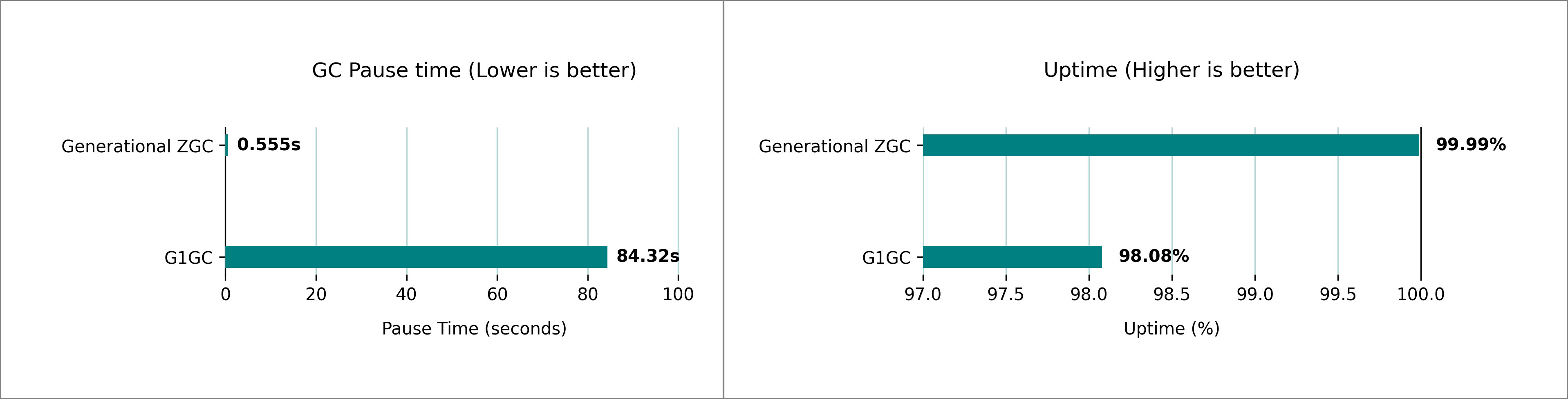
Our testing revealed significant differences in GC pause time between the generational ZGC and G1 GC for HBase on Amazon EMR 7.10. We used 1 m5.4xlarge (primary), 5 m5.4xlarge (core) nodes cluster settings and ran multiple iterations of 1-billion rows YCSB workloads to compare the GC pauses and uptime percentage. Based on our test cluster, we observed a GC pause time improvement from over 1 minute, 24 seconds, to under 1 seconds for over an hour-long execution, improving the application uptime from 98.08% to 99.99%.

We conducted extensive performance testing comparing G1 GC and generational ZGC on HBase clusters running on Amazon EMR, using the default heap settings automatically configured based on Amazon Elastic Compute Cloud (Amazon EC2) instance type. The following image shows the comparison in both GC pause time and uptime percentage at a peak load of 3,00,000 requests per second (data sampled over 1 hour).

Side-by-side comparison of Java garbage collectors showing Generational ZGC's superior pause time and uptime metrics versus G1GC

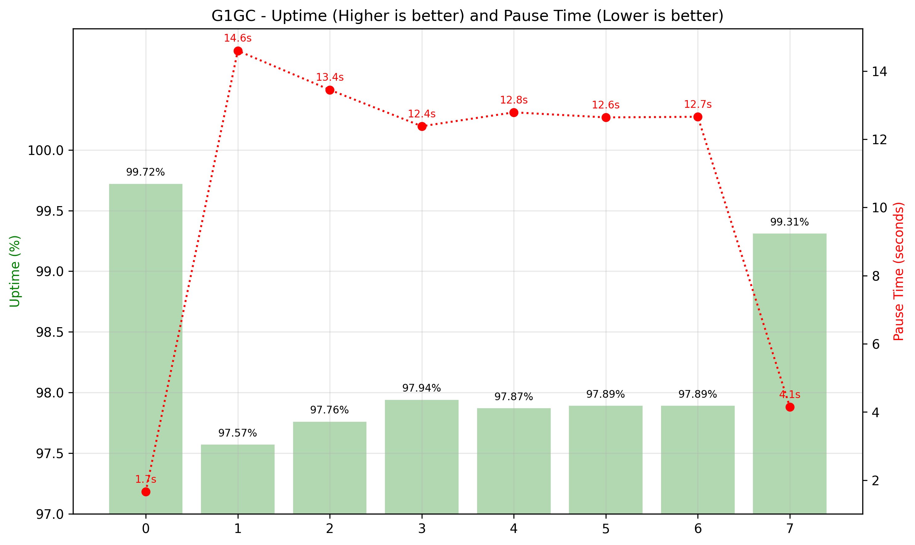
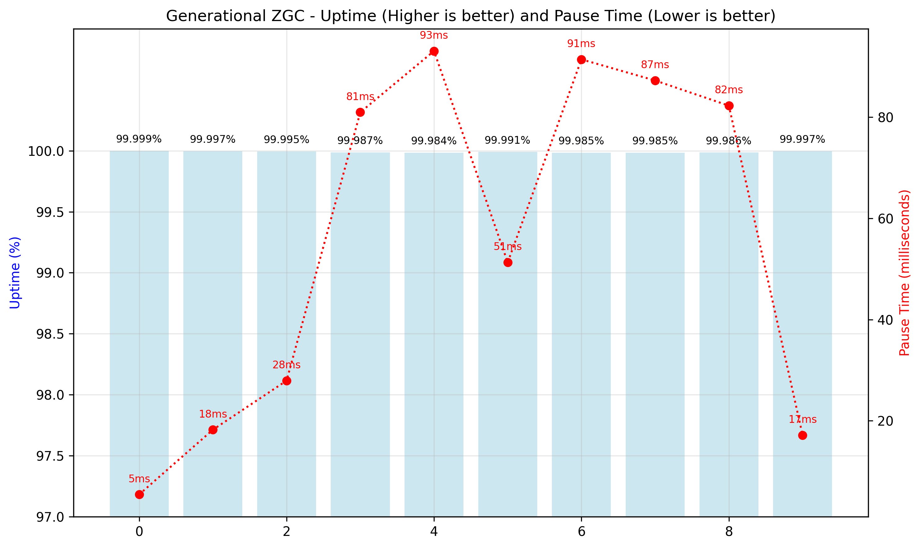
The following figures show the breakdown of the 1-hour runtime in 10-minute intervals. The left vertical axis measures the uptime, the right vertical axis measures the GC pause time, and the horizontal axis shows the interval. The generational ZGC maintained consistent uptime and pause time in milliseconds, and G1 GC demonstrated inconsistent and decreased uptime, pause times in seconds.

G1GC performance chart with dual y-axes: uptime percentage bars declining from 99.72% to 99.31%, and pause time trend peaking at 14.6s

Generational ZGC performance visualization with consistent uptime above 99.98% and fluctuating pause times peaking at 93ms

Tail latency comparison: Generational ZGC vs. G1GC in Amazon EMR HBase

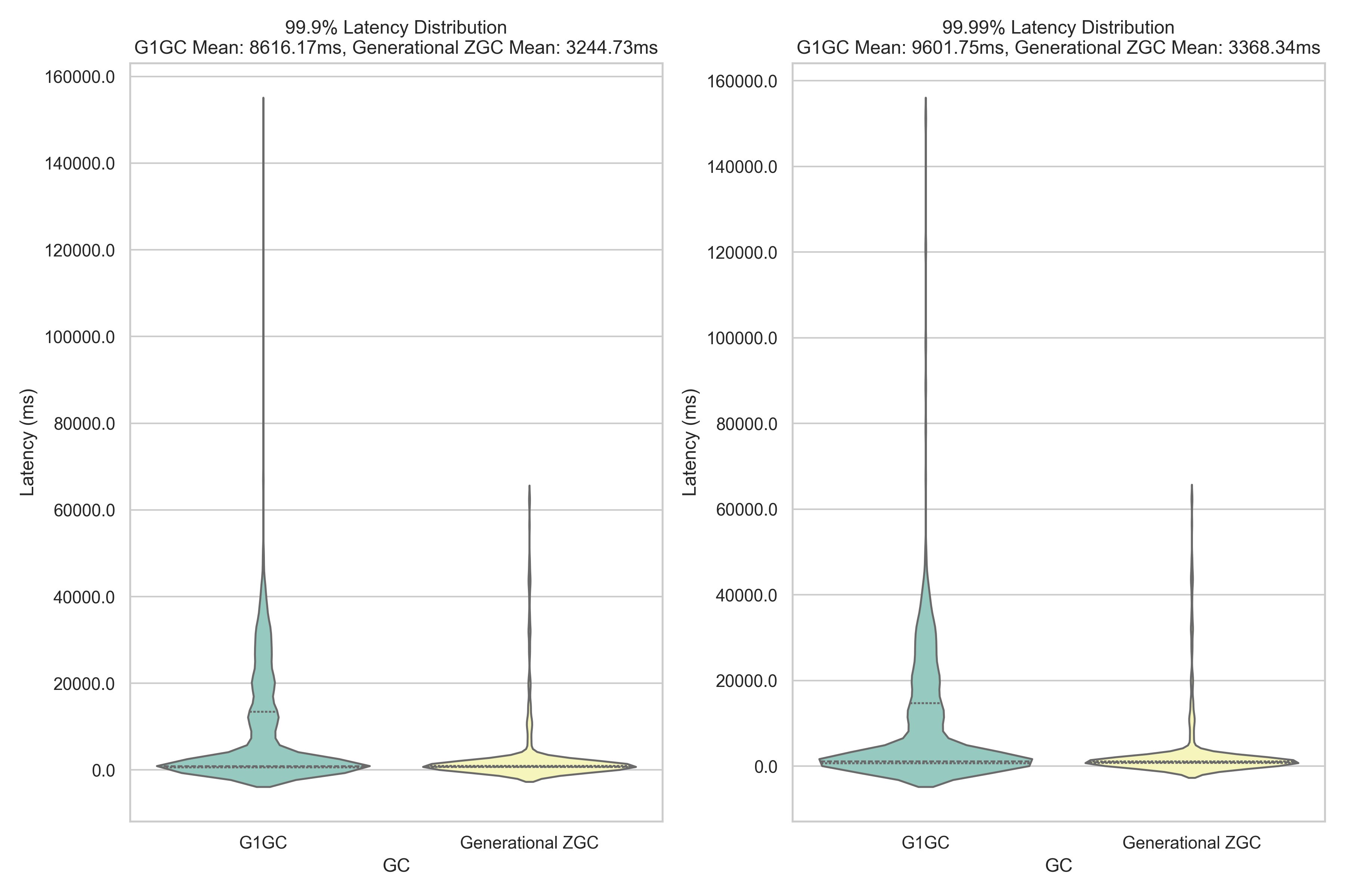
One of the most compelling advantages of generational ZGC over G1 GC is its predictable garbage collection behavior and the impact on application tail latency. G1 GC’s collection triggers are non-deterministic, meaning pause times can vary significantly and occur at unpredictable intervals. These unexpected pauses, though generally manageable, can create latency spikes that particularly affect the slowest percentile of operations. In contrast, generational ZGC maintains consistent, sub-millisecond pause times throughout its operation. This predictability proves crucial for applications requiring stable performance, especially at the highest percentiles of latency (99.9th and 99.99th percentiles). Our YCSB benchmark testing reveals the real-world impact of these different approaches. The following graph illustrates tail latency distribution between G1 GC and generational ZGC over a 2-hour sampling period :

Dual violin plot visualization comparing garbage collector latency distributions, demonstrating Generational ZGC's superior performance with lower mean latencies and tighter distribution

Improvements to BucketCache

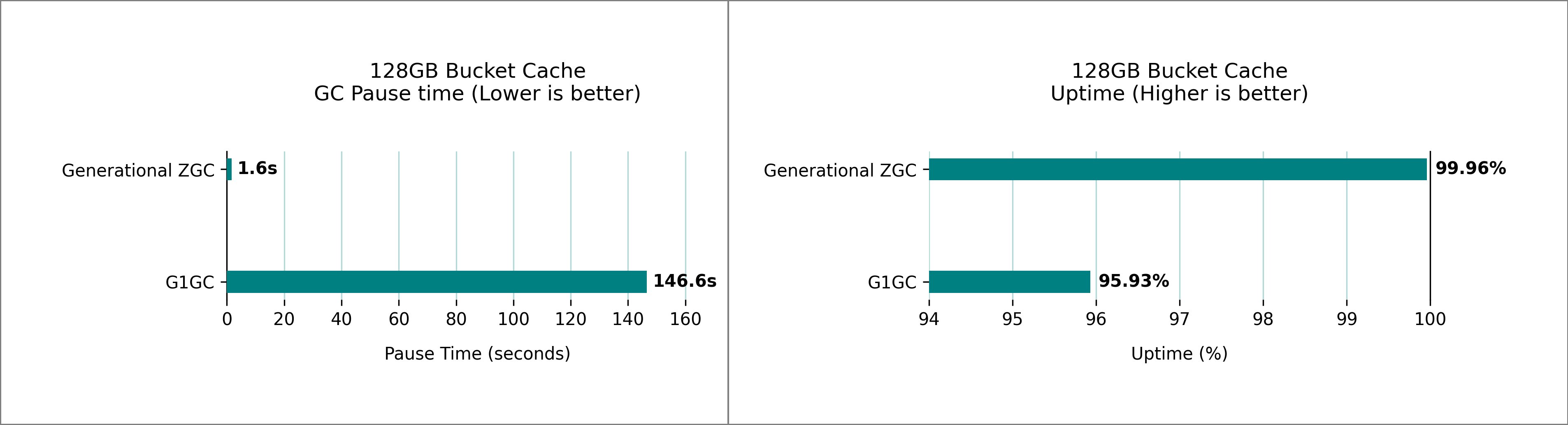
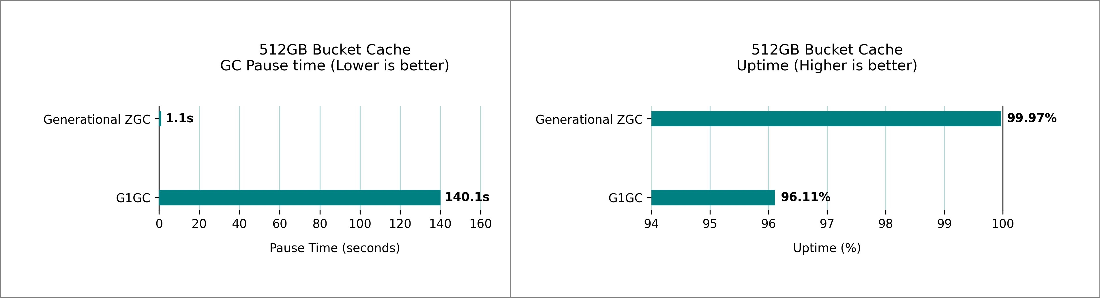
BucketCache is an off-heap cache in HBase that is used to cache the frequently accessed data blocks and minimize disk I/O. Bucket cache and heap memory works in conjunction and might increase the contention on the heap depending on the workload. Generational ZGC maintains it’s pause time goals even with a terabyte-sized bucket cache. We benchmarked multiple HBase clusters with varying bucket cache sizes and 32 GB RegionServer heap. The following figures show the peak pause times observed over a 1-hour sampling period, comparing G1 GC and generational ZGC performance.

128GB Bucket Cache performance metrics displaying Generational ZGC's superior pause times and uptime compared to G1GC implementation

Side-by-side performance metrics showing Generational ZGC's 1.1s pause time and 99.97% uptime versus G1GC's longer pauses and lower uptime

Enabling this feature and additional fine-tuning parameters

To enable this feature, follow the configurations mentioned in the Performance Considerations. In the following sections, we discuss additional fine-tuning parameters to tailor the configuration for your specific use case.

Fixed JVM heap 

Batch processing jobs and short-lived applications benefit from dynamic allocation’s ability to adapt to varying input sizes and processing demands when multiple applications co-exist on the same cluster and run with resource constraints. The memory footprint can expand during peak processing and contract when the workload diminishes. However, for production HBase deployments without any co-existing applications in the same fixed heap allocation offers stable, reliable performance.

Dynamic heap allocation is when the JVM flexibly grows and shrinks its memory usage between minimum (-Xms) and maximum (-Xmx) limits based on application needs, returning unused memory to the operating system. However, this flexibility comes at the cost of performance overhead and memory fragmentation. Dynamic allocation seemed flexible, but it created constant disruptions. The JVM was always negotiating with the operating system for memory, leading to performance overhead and fragmentation. On the other hand, fixed heap allocation pre-allocates a constant amount of memory for the JVM at startup and maintains it throughout runtime, providing better performance by reducing memory negotiation overhead with the operating system. To enable this feature, use the following configuration: :

[
    {
        "Classification": "hbase",
        "Properties": {
            "hbase.regionserver.fixed.heap.enabled": "true"
        }
    }
]

Enable pre-touch

Applications with large heaps can experience more significant pauses when the JVM needs to allocate and fault in new memory pages. Pre-touch (-XX:+AlwaysPreTouch) instructs the JVM to physically touch and commit all memory pages during heap initialization, rather than waiting until they’re first accessed during runtime. This early commitment reduces the latency of on-demand page faults and memory mappings that occur when pages are first accessed, resulting in more predictable performance especially during heavy load situations. By pre-touching memory pages at startup, you trade a slightly longer JVM startup time for more consistent runtime performance. To enable pre-touch for your HBase cluster, use the following configuration :

[
    {
        "Classification": "hbase-env",
        "Properties": {},
        "Configurations": [
            {
                "Classification": "export",
                "Properties": {
                    "JAVA_HOME": "/usr/lib/jvm/jre-21",
                    "HBASE_REGIONSERVER_GC_OPTS": "\"-XX:+UseZGC -XX:+ZGenerational -XX:+AlwaysPreTouch\""
                }
            }
        ]
    }
]

Increasing memory mappings for large heaps

Depending on the workload and scale, you might need to increase the Java heap size to accommodate large data in memory. When using the generational ZGC with a large heap setup, it’s critical to also increase the operating system’s memory mapping limit (vm.max_map_count).

When a ZGC-enabled application starts, the JVM proactively checks the system’s vm.max_map_count value. If the limit is too low to support the configured heap, it will issue the following warning :

[warning] The system limit on number of memory mappings per process might be too low for the given
[warning] max Java heap size (131072M). Please adjust /proc/sys/vm/max_map_count to allow for at
[warning] least 235929 mappings (current limit is 65530). Continuing execution with the current
[warning] limit could lead to a premature OutOfMemoryError being thrown, due to failure to map memory.

To increase the memory mappings, use the following configuration and adjust the count value in the command based on the heap size of the application.

echo "vm.max_map_count = 262144" | sudo tee -a /etc/sysctl.conf
sudo sysctl -p

sudo systemctl restart hbase-regionserver

Conclusion

The introduction of generational ZGC and fixed heap allocation for HBase on Amazon EMR marks a significant leap forward in the predictable performance and tail latency reduction. By addressing the long-standing challenges of GC pauses and memory management, these features unlock new levels of efficiency and stability for Amazon EMR HBase deployments. Although the performance improvements vary depending on workload characteristics, you can expect to see significant enhancements in your Amazon EMR HBase clusters’ responsiveness and stability. As data volumes continue to grow and low-latency requirements become increasingly stringent, features like generational ZGC and fixed heap allocation become indispensable. We encourage HBase users on Amazon EMR to enable these features and experience the benefits firsthand. As always, we recommend testing in a staging environment that mirrors your production workload to fully understand the impact and optimize configurations for your specific use case.

Stay tuned for more innovations as we continue to push the boundaries of what’s possible with HBase on Amazon EMR.


About the authors

Vishal Chaudhary is a Software Development Engineer at Amazon EMR. His expertise is in Amazon EMR, HBase and Hive Query Engine. His dedication towards solving distributed system problems is helping Amazon EMR to achieve higher performance improvements.

Ramesh Kandasamy is an Engineering Manager at Amazon EMR. He is a long tenured Amazonian dedicated to solve distributed systems problems.

Achieve low-latency data processing with Amazon EMR on AWS Local Zones

Post Syndicated from Gagan Brahmi original https://aws.amazon.com/blogs/big-data/achieve-low-latency-data-processing-with-amazon-emr-on-aws-local-zones/

Enterprises today require both single-digit millisecond latency data processing and data residency compliance for their applications. By deploying Amazon EMR on AWS Local Zones, organizations can achieve single-digit millisecond latency data processing for applications while maintaining data residency compliance. This post demonstrates how to use AWS Local Zones to deploy EMR clusters closer to your users, enabling millisecond-level response times. We use a Secure Web Gateway as an example and implement Amazon EMR with Apache Flink on AWS Local Zones to process network traffic with ultra-low latency. We also go through the process of creating an EMR cluster on AWS Local Zones, highlighting performance optimizations and architecture considerations specific to edge deployments. This approach uses AWS Local Zones to bring Amazon EMR’s data processing capabilities closer to your users and data sources – ideal for security applications or any other latency-sensitive workloads.

Solution overview

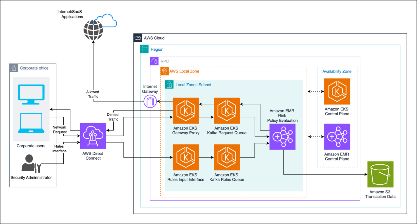
The following diagram illustrates the solution architecture.

Sample Architecture for Secure Web Gateway on AWS LocalZones

The solution consists of several key components:

  • AWS Local Zones deployment – Positioned close to corporate offices to minimize latency
  • Network traffic interception – Using AWS Transit Gateway and virtual private cloud (VPC) endpoints
  • Request queuing and rules streaming – Using Apache Kafka on Amazon Elastic Kubernetes Service (Amazon EKS) to queue the incoming and outgoing network requests as well as stream rules as they are updated by the security administrator
  • EMR cluster – Running Flink for real-time stream processing and functions to combine rules
  • Policy management system – For defining and updating security rules
  • Logging – Using Amazon Simple Storage Service (Amazon S3) for visibility, compliance, and data analytics

In this scenario, the Secure Web Gateway is designed to inspect and make decisions on network traffic within single-digit milliseconds. The workflow consists of the following steps:

  1. The corporate office uses AWS Direct Connect to connect to AWS Local Zones.
  2. The security administrator defines the rules from a rules interface running on Kubernetes pods on Amazon EKS. As the rules are added or modified, they are sent to the swg_rules Kafka topic running on Amazon EKS. These rules are stored and processed by Flink running on the EMR cluster.
  3. A corporate user requests for a software as a service (SaaS) application from the corporate office. The request is routed through Direct Connect to the Local Zone.
  4. The Secure Web Gateway proxy service running on Kubernetes pods on Amazon EKS receives the access request, which is sent to the swg_requests Kafka topic.
  5. Flink running on EMR evaluates and consumes the messages from the swg_requests Kafka topic and determines the routing decision, which is sent back to the swg_decisions Kafka topic.
  6. The Secure Web Gateway proxy service consumes the swg_decisions topic and routes the traffic to the SaaS application, if the access request is allowed. If the request is denied, the proxy responds back to the users with the reason or violations details, if any.

Due to the real-time nature of the solution, the security administrator can add, modify, or remove the rules through the swg_rules topic as Flink constantly consumes and evaluates this topic.In the following sections, we discuss the key components of the solution in more detail.

AWS Local Zones: The foundation

AWS Local Zones provide low-latency extensions of AWS Regions positioned near large population and industry centers. For our Secure Web Gateway use case, deploying in a Local Zones offers several advantages:

  • Proximity to corporate offices – Reducing round-trip latency for traffic inspection. AWS Local Zones is designed to provide applications with low latency aiming for single-digit millisecond performance.
  • AWS-native security controls – Using AWS security features.
  • Consistent connectivity – Reliable connection between corporate networks and AWS resources.

The Local Zone hosts our EMR cluster and networking components, making sure traffic inspection through the Secure Web Gateway happens with single-digit millisecond latency. For scenarios where traffic inspection doesn’t require single-digit millisecond latency, deploying hosting the solution on EMR cluster in a Region should work fine.

Amazon EMR with Apache Flink: The decision engine

The core intelligence of our Secure Web Gateway solution is powered by Amazon EMR running Flink for real-time stream processing. With Amazon EMR running on Flink, we take advantage of the optimized real-time stream processing capability offered by Flink. EMR running in AWS Local Zones helps users perform complex data processing closer to their data centers or corporate locations without worrying any potential latency introduced for moving the data to other Regions. In this particular solution, we use Flink’s stateful processing, which allows for maintaining the session context across multiple network requests/packets. The solution also provides a dynamic rules engine that is combined with the real-time stream of requests for network access.

Architectural component choice considerations

Amazon EMR offers several deployment options for different kinds of workloads and use cases, including Amazon EMR on EKS. AWS also provides Amazon Managed Service for Apache Flink, a fully managed service that simplifies the process of building and managing Flink applications. As of this writing, both the EMR on EKS deployment option and Amazon Managed Service for Apache Flink are not available in AWS Local Zones.

Prerequisites

Before proceeding with this deployment, ensure you have:

  • AWS account with AWS IAM permissions for Amazon VPC, EMR, and Local Zones management
  • Basic familiarity with the AWS Management Console

Deploy Amazon EMR on a Local Zone

To deploy Amazon EMR on a Local Zone, you first need to enable the Local Zone for the AWS account. For instructions, refer to Step 1 and Step 2 in Getting started with AWS Local Zones.

After you have enabled a Local Zone and created a Local Zone subnet, create your EMR cluster. For instructions, refer to Step 1: Configure data resources and launch an Amazon EMR cluster. You can follow the instructions provided for the AWS Management Console. Make sure you select the appropriate Amazon EMR release version (5.28.0 or later for Local Zone support). Select the applications you need, which in this case is Hadoop and Flink.

A crucial step to launching an EMR cluster in a Local Zone is selecting the Local Zone network configuration. Choose the VPC that contains your Local Zone subnet, and choose the subnet that you created in the Local Zone.

Review all other configurations and settings for your cluster and make any final adjustments as needed, then choose Create cluster to launch your EMR cluster in the Local Zone.

Performance and scaling considerations

The Local Zone EMR deployment can be scaled based on traffic patterns. You can manually scale the EMR cluster horizontally by adding more worker nodes during peak traffics to provide low-latency performance, after you have increased the number of users that access the Secure Web Gateway. Alternatively, you can set up a scheduled action to scale the EMR cluster at predetermined times based on known workload patterns. You can also perform vertical scaling by using Amazon Elastic Compute Cloud (Amazon EC2) instance types with more compute capacity. Consider using the manual resize option for EMR clusters to modify the cluster size based on workload requirements.

Another important performance consideration is to optimize Flink checkpointing for fault tolerance. To learn more, see Optimizing job restart times for task recovery and scaling operations.

Security considerations

Although this architecture prioritizes low-latency performance, implementing proper security controls is essential for production deployments. The solution handles sensitive corporate network traffic that requires protection through encryption, access controls, and monitoring. For comprehensive security guidance specific to EMR deployments, refer to Security in Amazon EMR. Consider the following key areas:

  • Data protection – Enable encryption at rest and in transit using Amazon EMR security configurations, including Amazon S3 encryption and TLS certificates for inter-node communication
  • Access control – Implement AWS Identity and Access Management (IAM) roles with least privilege for Amazon EMR service roles, EC2 instance profiles, and runtime roles to isolate job access
  • Network security – Deploy EMR clusters in private subnets with security groups following least privilege, and enable the Amazon EMR block public access feature

Benefits of Amazon EMR

Using Amazon EMR on AWS Local Zones in this architecture offers several key benefits:

  • Low latency – Providing the compute in AWS Local Zones close to corporate offices helps you achieve low-latency processing.
  • Real-time inspection – Flink’s streaming capabilities unlocks the ability to process real-time inspection for network requests.
  • Complex policy application – With Flink on Amazon EMR, you can build a complex policy application that, for instance, can detect sophisticated access patterns across multiple events and time windows that would be impossible with traditional rule-based systems.
  • Scalability – Amazon EMR provides the flexibility to automatically scale the cluster with a custom policy. Moreover, Amazon EMR release 6.15.0 and higher supports Flink autoscaler, which automatically scales the individual Flink job vertexes based on the job metrics.
  • Compliance – Logging all the events to a durable storage like Amazon S3 helps users improve their security and audit posture.

Clean up

To avoid incurring unnecessary charges, clean up the resources you created during this walkthrough. Follow these steps in order:

Step 1: Terminate the EMR cluster

  • Open the Amazon EMR console
  • Select your EMR cluster from the list
  • Choose Terminate
  • Confirm the termination when prompted
  • Wait for the cluster status to change to “TERMINATED”

Step 2: Clean up VPC resources

  • In the Amazon VPC console, delete the Local Zone subnet you created
  • If you created a custom VPC specifically for this demo, delete any associated:
    • Route tables
    • Internet gateways
    • Security groups (other than default)
    • The VPC itself

Step 3: Disable the Local Zone (optional)

  • In the EC2 console, go to Zones under “Settings”
  • Find your enabled Local Zone
  • Choose Manage and disable the zone if you no longer need it for other workloads

Step 4: Review additional resources Check for and clean up any other resources you may have created:

  • S3 buckets used for logging or EMR storage
  • CloudWatch log groups
  • Any custom IAM roles or policies created specifically for this architecture

Conclusion

This implementation of Amazon EMR on AWS Local Zones demonstrates how enterprises can bring powerful data processing capabilities to the edge while maintaining single-digit millisecond latency. By showcasing a Secure Web Gateway application, we have illustrated just one of many possible use cases where performance-sensitive workloads can benefit from this architecture.As the edge computing landscape evolves, we anticipate organizations will increasingly use this pattern for additional use cases, including:

  • Real-time fraud detection for financial transactions requiring immediate decision-making
  • Connected vehicle applications where processing telemetry data with minimal latency is critical
  • Internet of Things (IoT) sensor analytics that require immediate insights from operational technology environments
  • Augmented reality experiences where processing must happen close to end-users

We encourage you to evaluate your latency-sensitive workloads and consider how AWS Local Zones with Amazon EMR might help you implement architectures previously perceived highly challenging. Start small with a proof of concept like the one outlined here, measure the performance gains, and expand to production use cases with confidence. Implementing a Secure Web Gateway in AWS Local Zones with Amazon EMR and Flink offers enterprises a powerful solution for securing corporate traffic. By using the proximity of Local Zones and the real-time processing capabilities of Flink, organizations can implement sophisticated security policies without the latency penalties traditionally associated with traffic inspection.


About the authors

Gagan Brahmi is a Specialist Senior Solutions Architect at Amazon Web Services (AWS), specializing in Data Analytics and AI/ML solutions. With over 20 years in information technology, he helps customers architect scalable, high-performance analytics platforms using distributed data processing, real-time streaming technologies, and machine learning services on AWS. When not designing cloud solutions, Gagan enjoys exploring new places with his family.

Arun Shanmugam is a Senior Analytics Solutions Architect at AWS, with a focus on building modern data architecture. He has been successfully delivering scalable data analytics solutions for customers across diverse industries. Outside of work, Arun is an avid outdoor enthusiast who actively engages in CrossFit, road biking, and cricket.

George Oakes is a Senior Hybrid Solutions Architect at AWS, with a focus on edge, on-premise, and low latency architectures. He has been successfully delivering scalable hybrid AWS solutions for customers across diverse industries. Outside of work, George is an avid outdoor enthusiast who enjoys hiking and visiting parks and UNESCO sites around.

Enhance Amazon EMR observability with automated incident mitigation using Amazon Bedrock and Amazon Managed Grafana

Post Syndicated from Yu-Ting Su original https://aws.amazon.com/blogs/big-data/enhance-amazon-emr-observability-with-automated-incident-mitigation-using-amazon-bedrock-and-amazon-managed-grafana/

Maintaining high availability and quick incident response for Amazon EMR clusters is important in data analytics environments. In this post, we show you how to build an automated observability system that combines Amazon Managed Grafana with Amazon Bedrock to detect and remediate EMR cluster issues. We demonstrate how to integrate real-time monitoring with AI-powered remediation suggestions, combining Amazon Managed Grafana for visualization, Amazon Bedrock for intelligent response recommendations, and AWS Systems Manager for automated remediation actions on Amazon Web Services (AWS).

Solution overview

This solution helps you improve EMR cluster observability through a comprehensive four-layer architecture—comprising monitoring, notification, remediation, and knowledge management—to provide the following features:

  • Real-time monitoring of EMR clusters using Amazon Managed Service for Prometheus and Amazon Managed Grafana
  • Automated first-aid remediation through Systems Manager
  • AI-powered incident response suggestions using Amazon Bedrock
  • Integration with the AWS Premium Support knowledge base
  • Historical incident data archival and analysis

The implementation of this architecture delivers the following key benefit:

  • Reduced Mean time to resolution (MTTR)
  • Proactive incident prevention
  • Automated first-response actions
  • Knowledge base enrichment through machine learning

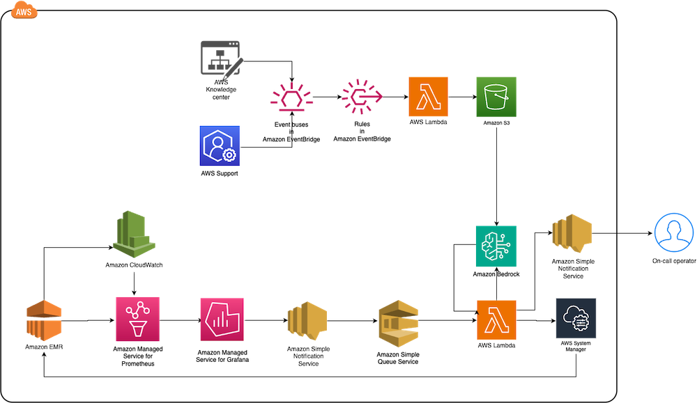
The following diagram illustrates the solution architecture.

End-to-end AWS monitoring solution diagram integrating Knowledge Center, Support, CloudWatch metrics with EventBridge rules and Lambda processing

The architecture comprises the following core components:

  • Monitoring layer – The monitoring layer uses Amazon Managed Service for Prometheus and Amazon CloudWatch to capture real-time metrics from EMR clusters. Amazon Managed Grafana serves as the visualization layer, offering comprehensive dashboards for Apache YARN, HDFS, Apache HBase, and Apache Hudi performance monitoring. Advanced alerting mechanisms trigger notifications based on predefined query results.
  • Notification layer – To provide timely and reliable alert delivery, the notification layer uses Amazon Simple Notification Service (Amazon SNS) for distribution and Amazon Simple Queue Service (Amazon SQS) for message queuing. This architecture prevents message delays and provides a robust trigger mechanism for AWS Lambda functions.
  • Remediation layer – The remediation layer enables automatic issue resolution through:
    • Lambda functions for orchestration
    • Systems Manager for script execution
    • Amazon Bedrock (amazon.nova-lite-v1:0) for generating intelligent response recommendations
  • Knowledge management layer – To maintain an up-to-date knowledge base, the solution:

We provide an AWS CloudFormation template to deploy the solution resources.

Prerequisites

Before starting this walkthrough, make sure you have access to the following AWS resources and configurations:

  • An AWS account
  • Access to the US East (N. Virginia) AWS Region
    • Add access to Amazon Bedrock foundation models (amazon.nova-lite-v1:0)

  • Amazon EMR version 6.15.0 (used in this demo)
  • Archived technical or troubleshooting articles
  • AWS IAM Identity Center enabled with at least one role that can become a Grafana administrator
  • (Optional) AWS Premium Support with a business support plan or higher for enhanced troubleshooting capabilities

Throughout this walkthrough, we provide detailed instructions to set up and configure these prerequisites if you haven’t already done so.

Configure resources using AWS CloudFormation

Complete the following steps to configure your resources:

  1. Launch the CloudFormation stack:

launch stack

  1. Provide emrobservability as the stack name.
  2. Select a virtual private cloud (VPC) and assign a public subnet.
  3. For EMRClusterName, enter a name for your cluster (default: emrObservability).
  4. Enter an existing Amazon S3 location as the Apache HBase root directory location (for example, s3://mybucket/my/hbase/rootdir/).
  5. For MasterInstanceType and CoreInstanceType, enter your instance types (default: m5.xlarge for both).
  6. For CoreInstanceCount, enter your instance count (default: 2).
  7. For SSHIPRange, use CheckIp and enter your IP (for example, 10.1.10/32).
  8. Choose the release label (default: 6.15.0).
  9. For KeyName, enter a key name to SSH to Amazon Elastic Compute Cloud (Amazon EC2) instances.
  10. For LatestAmiId, enter your AMI (default: /aws/service/ami-amazon-linux-latest/amzn2-ami-hvm-x86_64-gp2).
  11. For KBS3Bucket, enter a name for your S3 bucket (for example, mykbbucket).
  12. For SubscriptionEndpoint, enter an email address to receive notifications and responses (for example, [email protected]).

Accept subscription confirmation

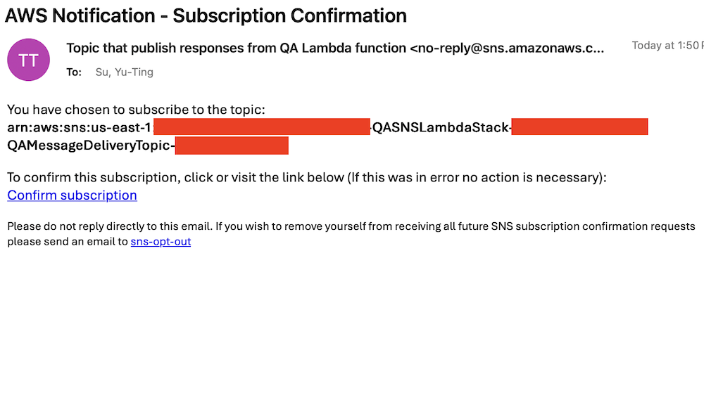
Accept the subscription confirmation sent to the email address you specified in the CloudFormation stack parameters. The following screenshot shows an example of the email you receive.

AWS email confirmation for SNS topic subscription to QA Lambda function responses with opt-out instructions

Prepare the knowledge base

Complete the following steps to populate the S3 bucket with archived technical articles and cases:

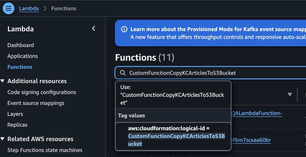
  1. On the Lambda console, choose Functions in the navigation pane.
  2. Choose the function CustomFunctionCopyKCArticlesToS3Bucket.

AWS Lambda console displaying Functions page with CustomFunctionCopyKCArticlesToS3Bucket function details

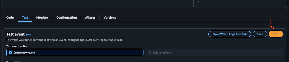
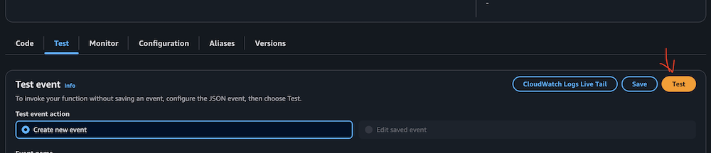
  1. Manually invoke the function by choosing Test on the Test tab.

AWS Lambda Test tab interface with event configuration options

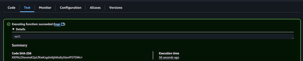
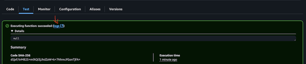
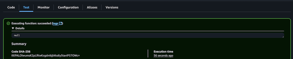
  1. Verify successful execution by checking the CloudWatch logs.

AWS Lambda successful function execution result with null output

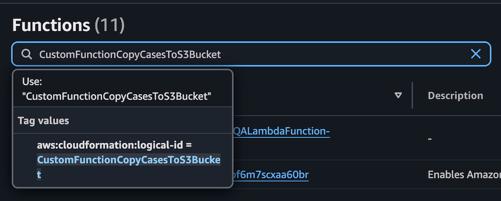
  1. Repeat the process for the Lambda function CustomFunctionCopyCasesToS3Bucket.

Lambda function interface displaying CustomFunctionCopyCasesToS3Bucket configuration with CloudFormation ID and description panel

AWS Lambda test interface showing Test event configuration options and action buttons

AWS Lambda function execution success message with null response and SHA-256 code

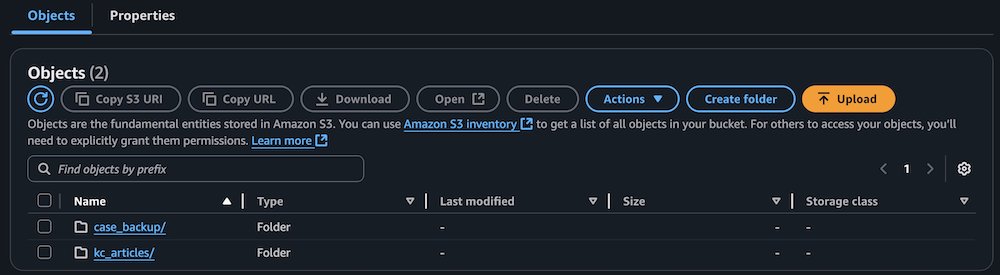
  1. Confirm the S3 bucket has been populated with archived technical articles and cases.

Amazon S3 bucket interface showing two folders with action buttons and search functionality

Sync data to the Amazon Bedrock knowledge base

Complete the following steps to sync the data to your knowledge base:

  1. On the Lambda console, choose Functions in the navigation pane.
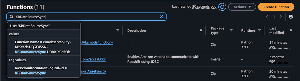
  2. Choose the function KBDataSourceSync.

AWS Lambda console displaying filtered functions with CloudFormation tags, Python runtime versions, and modification timestamps

  1. Manually invoke the function by choosing Test on the Test tab.

This task might take 10–15 minutes to complete.

AWS Lambda console test configuration panel with CloudWatch integration and event creation controls

  1. Verify successful execution by checking the CloudWatch logs.

Lambda function execution results showing successful completion status and details

Configure your Amazon Managed Grafana workspace

Complete the following steps to configure your Amazon Managed Grafana workspace:

  1. On the Amazon Managed Grafana console, choose Workspaces in the navigation pane.
  2. Open your workspace.
  3. Choose Assign new user or group.

Amazon Grafana workspace showing IAM configuration notice and user assignment button

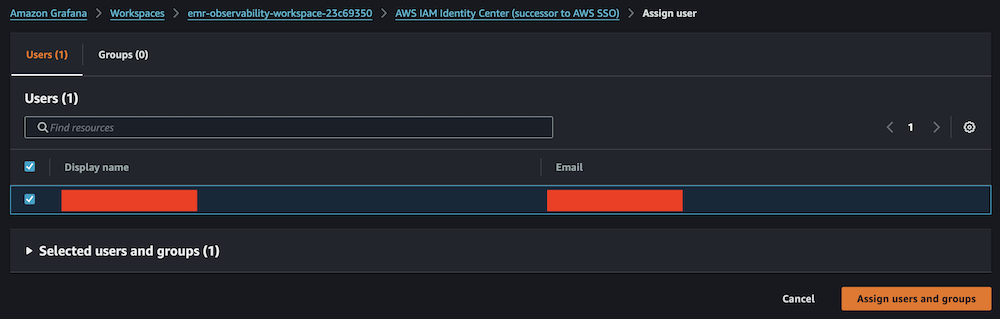
  1. Select your IAM Identity Center role and choose Assign users and groups.

Amazon Grafana IAM Identity Center user assignment panel with search and selection controls

  1. On the Admin dropdown menu, choose Make admin.

Amazon Grafana user list showing assigned viewer with admin action options

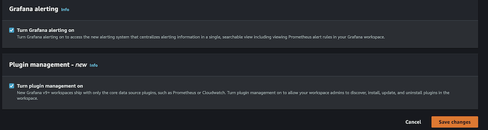
  1. Enable Grafana alerting, then choose Save changes.

Amazon Grafana alerting configuration panel showing disabled status with navigation tabs and edit button

Amazon Grafana configuration panel showing enabled alerting and plugin management settings

  1. Wait 10 minutes for the workspace to become active.
  2. When it’s active, sign in to the Grafana workspace. (For more information, refer to Connect to your workspace.)

Configure data sources

Add and configure the following data sources:

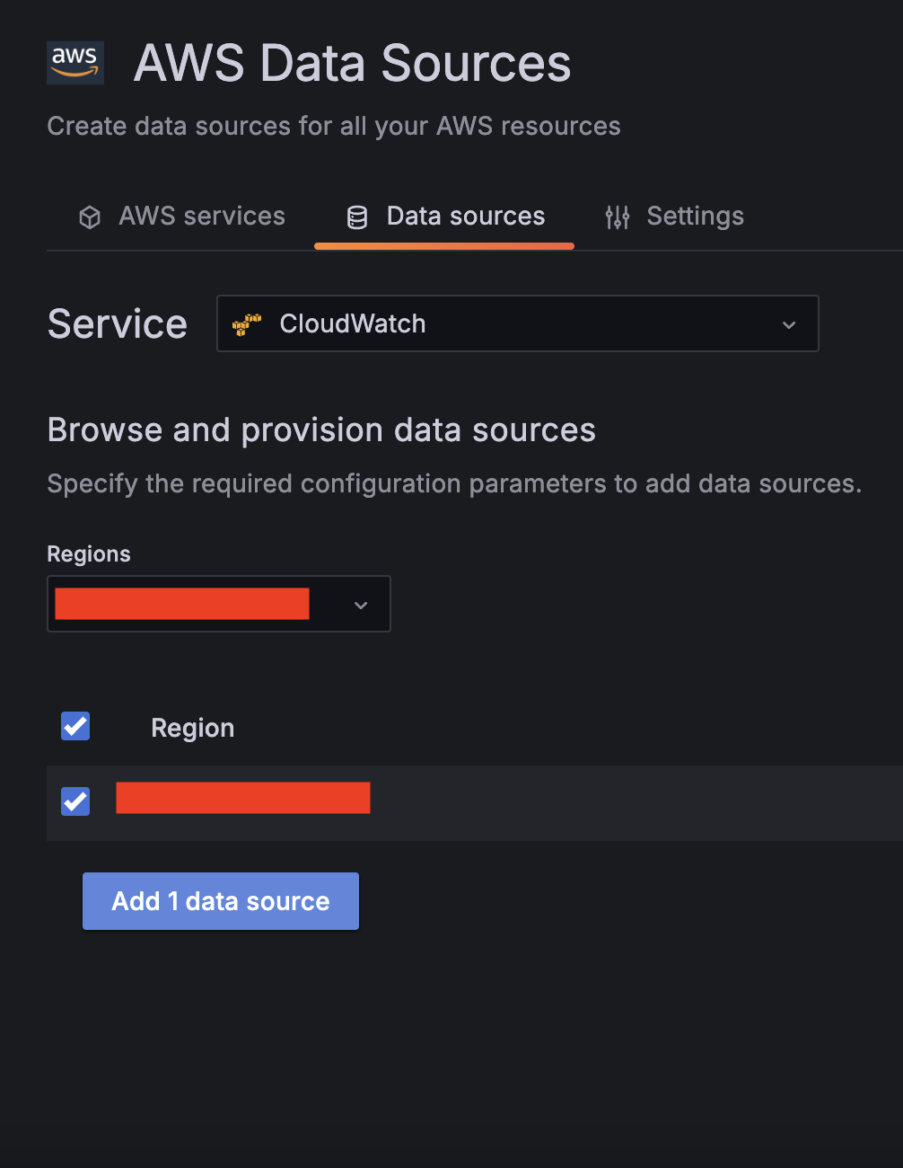
  1. For Service, choose CloudWatch, then select your Region and add CloudWatch as a data source.

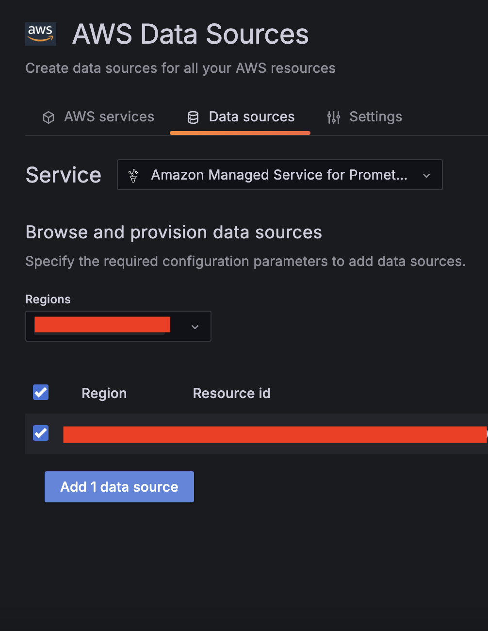
  1. Choose Amazon Managed Service for Prometheus as a second data source and select your Region.

  1. Validate CloudWatch connectivity:
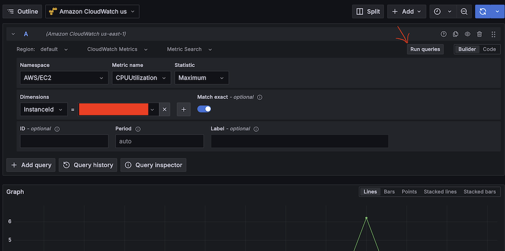
    1. Run test queries (for example, Namespace: AWS/EC2, Metric name: CPUUtilization, Statistic: Maximum).
      Amazon Managed Gragana interface showing CPU utilization query setup for EC2 instance.
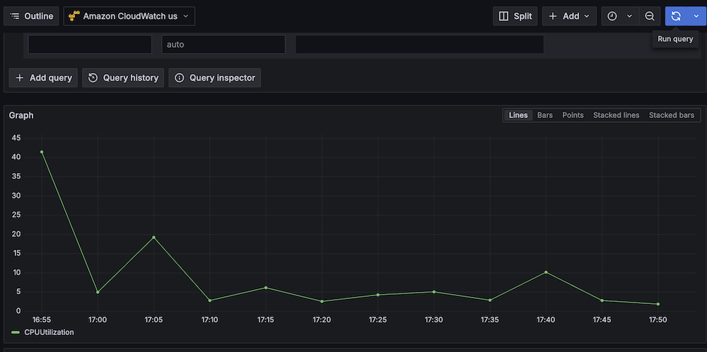
    2. Verify CloudWatch metric retrieval.
      Line graph showing CPU utilization over time with peak at 40%.
  1. Validate Amazon Managed Service for Prometheus connectivity:
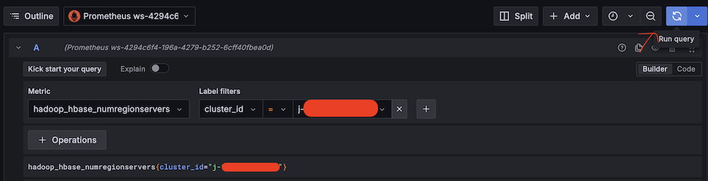
    1. Run test queries (for example, Metric: hadoop_hbase_numregionservers, Label filters: cluster_id = <Amazon EMR cluster ID>).
      Amazon Managed Grafana query interface showing Hadoop HBase metric configuration.
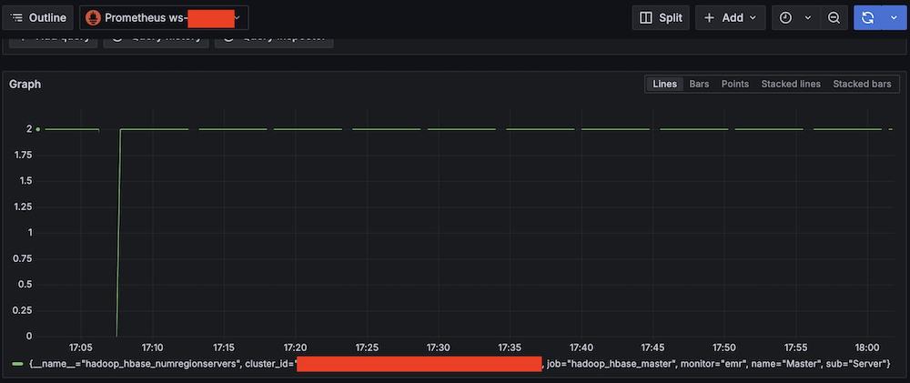
    2. Verify Prometheus metric retrieval.
      Amazon Managed Grafana monitoring dashboard showing a graph with HBase Region Server amount from 0 to 2

Confirm SNS notification channels

Complete the following steps to confirm your SNS notification is set up:

  1. On the Amazon SNS console, choose Topics in the navigation pane.
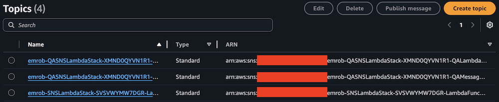
  2. Locate and note the ARNs for -LambdaFunctionTopic and -QALambdaFunctionTopic.

AWS SNS Topics list showing 4 topics with names, types, and ARNs

AWS SNS Topics console showing filtered search results for "LambdaFunctionTopic"

AWS SNS Topics console showing filtered search results for "QALambdaFunctionTopic"

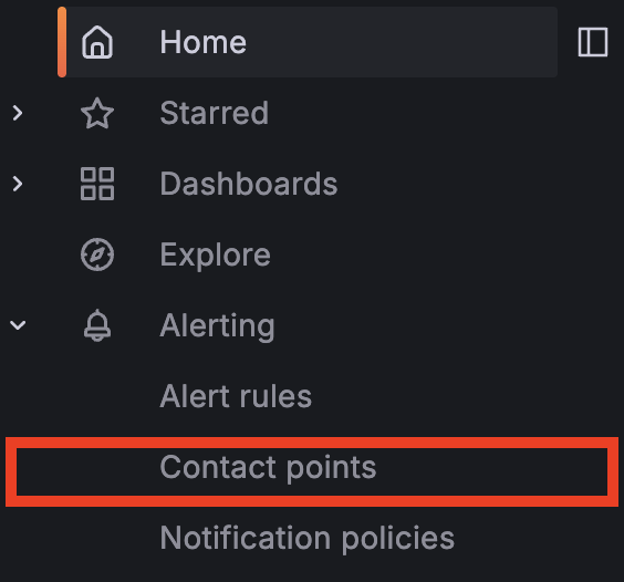
  1. Choose Contact points under Alerting.

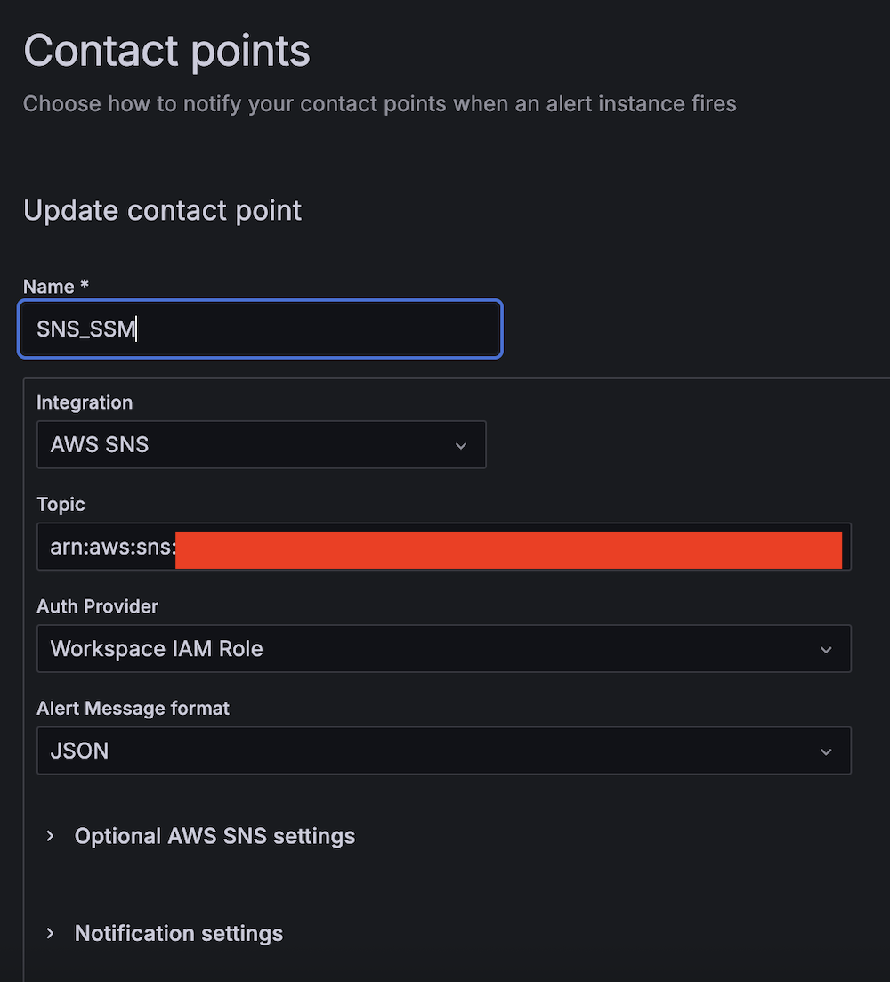
  1. Create the first contact point:
    1. For Name, enter SNS_SSM.
    2. For Integration, choose AWS SNS.
    3. For Topic, enter the ARN for LambdaFunctionTopic.
    4. For Auth Provider, choose Workspace IAM role.
    5. For Alert Message format, choose JSON.

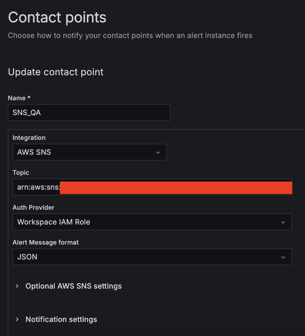
  1. Create the second contact point:
    1. For Name, enter SNS_QA.
    2. For Integration, choose AWS SNS.
    3. For Topic, enter the ARN for QALambdaFunctionTopic.
    4. For Auth Provider, choose Workspace IAM role.
    5. For Alert Message format, choose JSON.

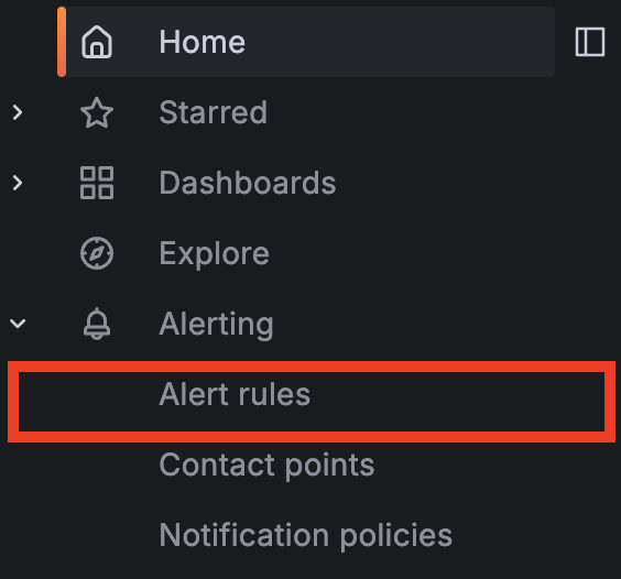
Create alert rules

Complete the following steps to set up two critical alert rules:

  1. Choose Alert rules under Alerting.

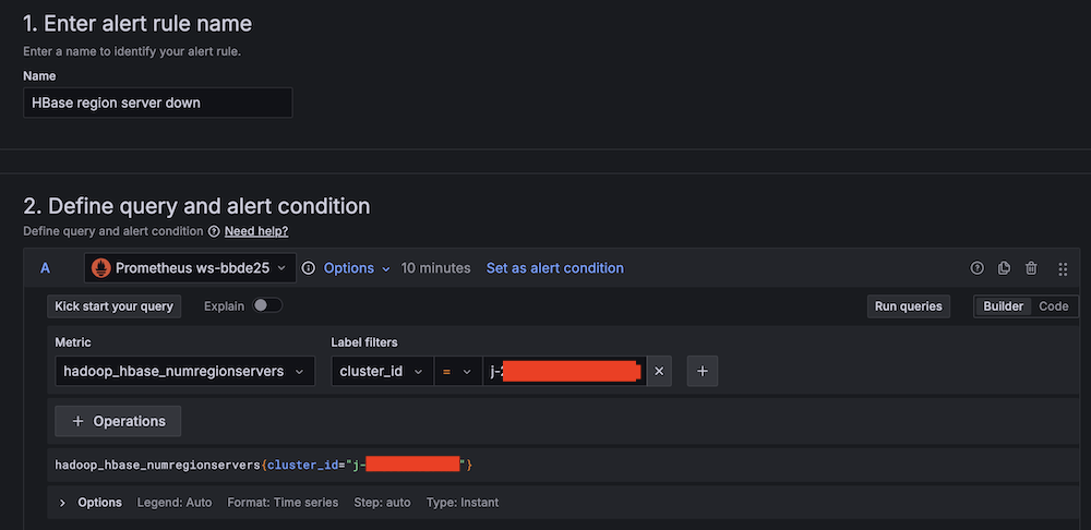
  1. Set up alerting if the Apache HBase region server status is abnormal:
    1. For Alert name, enter HBase region server down.
    2. For Data source, choose Amazon Managed Service for Prometheus.
    3. For Metric, choose hadoop_hbase_numregionservers.
      Alert rule configuration interface for HBase region server monitoring
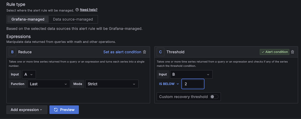
    4. For Threshold, configure to alert if the region server count is less than 2 for 3 minutes.
      Amazon Managed Grafana alert rule configuration interface with expressions setup
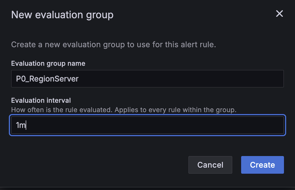
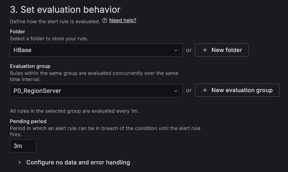
    5. For Evaluation interval, set to 1 minute.
      New evaluation group creation modal showing P0_RegionServer name input and 1m interval settingHBase alert configuration panel showing P0_RegionServer group and 3m pending period
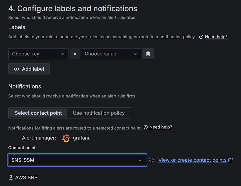
    6. For Contact point, choose SNS_SSM.
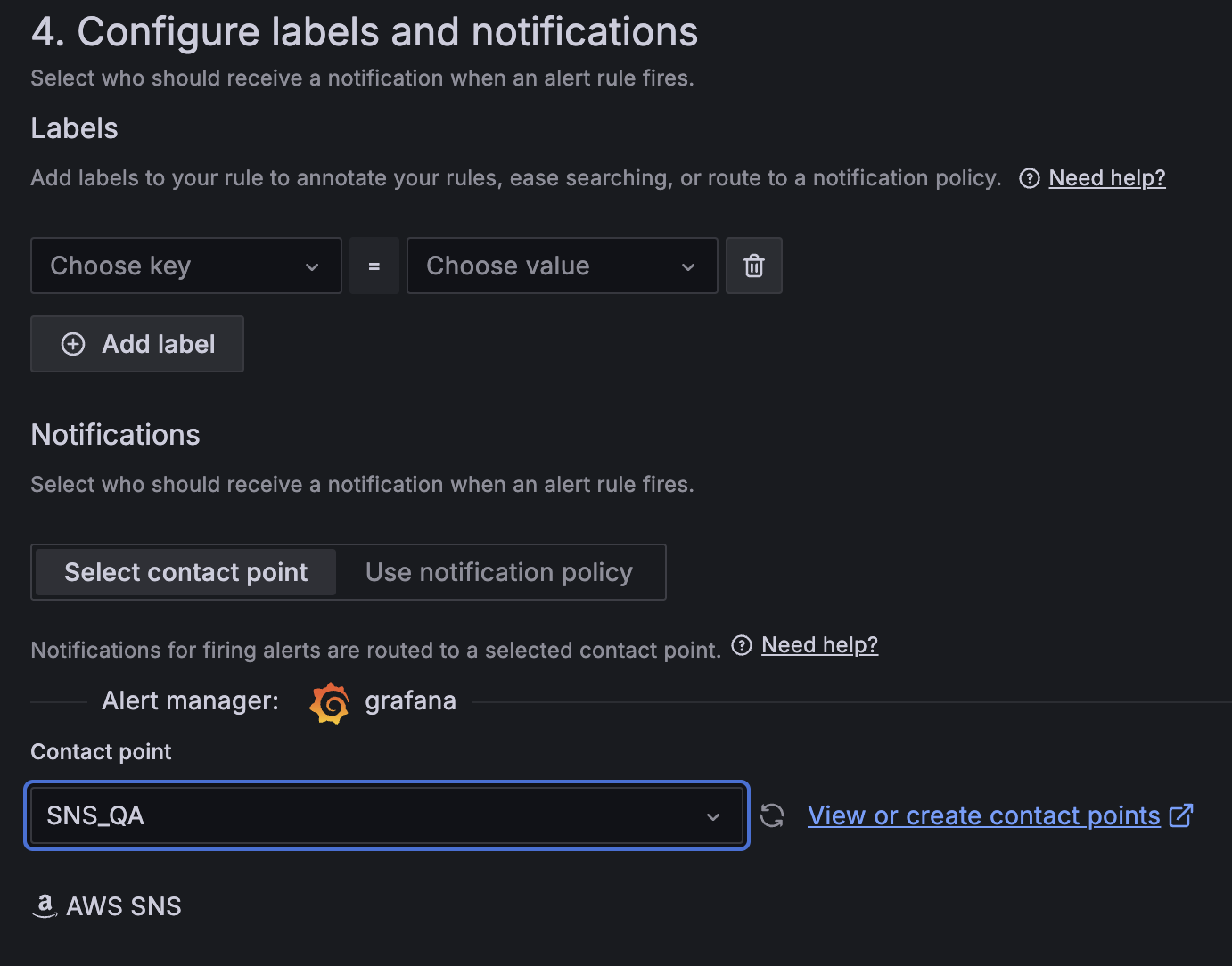
      Amazon Managed Grafana alert configuration interface showing labels and notifications setup with AWS SNS integration
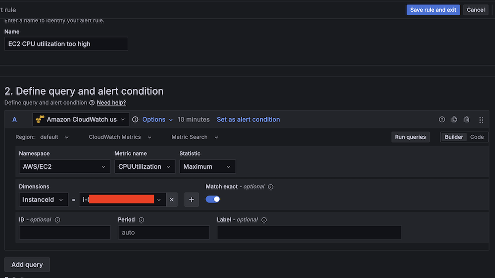
  1. Create a second alert for if Amazon EC2 CPU utilization is abnormal:
    1. For Alert name, enter EC2 CPU utilization too high.
    2. For Data source, choose Amazon CloudWatch.
    3. For Namespace, choose AWS/EC2.
    4. For Metric name, choose CPUUtilization
    5. For Statistic, choose Maximum.
      Amazon CloudWatch query interface for setting up EC2 CPU utilization alert conditions
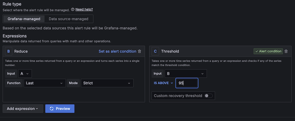
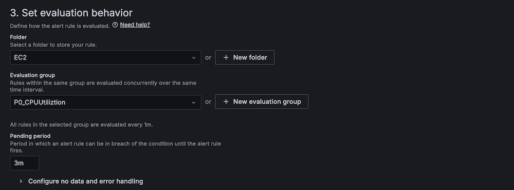
    6. For Threshold, configure to alert if CPU utilization is more than 95% for 3 minutes.
      Amazon Managed Grafana alert interface with Reduce and Threshold expressions for alert condition management
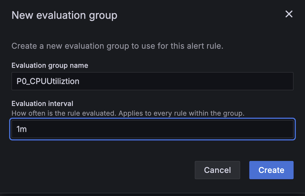
    7. For Evaluation interval, configure to 1 minute.
      New evaluation group configuration modal showing CPU utilization monitoring setup with 1-minute interval
      AWS Managed Grafana alert rule configuration screen showing evaluation behavior settings
    8. For Contact point, choose SNS_QA.Amazon Managed Grafana alert configuration showing customizable labels, contact point selection for SNS_QA integration
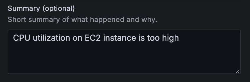
  1. On the alert rule creation page, scroll to 5. Add annotations and for Summary, add a clear description of the alert, for example, CPU utilization on EC2 instance is too high.

Alert configuration summary field with "CPU utilization on EC2 instance is too high" warning message

Apache HBase region server incident test

To confirm the system is working as expected, complete the following Apache HBase region server incident test:

  1. SSH into an EMR core instance.
  2. Stop the Apache HBase region server using systemctl:
 # Stop HBase region server service 
 sudo systemctl stop hbase-regionserver.service 

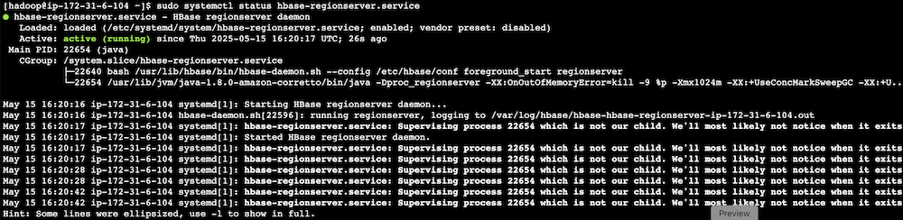
  1. Verify the service status:
 # Check the current state of HBase region server service 
 sudo systemctl status hbase-regionserver.service
  1. Observe Amazon Managed Grafana alert progression:
    1. Monitor alert status changes.
      Alert dashboard showing HBase region server alert status in pending state
      Alert dashboard showing HBase region server alert in firing state
    2. Verify SNS message generation.
    3. Confirm SQS message queuing.
    4. Track the Lambda function triggered for remediation.

Terminal output showing HBase RegionServer service status and daemon processes

HBase monitoring interface displaying region server status with health indicators and action buttons

CPU utilization stress test

Complete the following CPU utilization stress test:

  1. SSH into the EMR primary instance.
  2. Install stress testing tools:
 sudo amazon-linux-extras install epel -y
 sudo yum install stress -y 

  1. Verify the installation:
 stress --version 

  1. Generate high CPU load using the stress command and the following command structure:
 sudo stress [options] 

For our Amazon EMR test, use the following command:

 # For m5.xlarge instances (4 vCPUs) sudo stress --cpu 4 

-c 4 in the command creates 4 CPU-bound processes (one for each vCPU).The following are instance type vCPUs for your reference:

  • m5.xlarge: 4 vCPUs
  • m5.2xlarge: 8 vCPUs
  • m5.4xlarge: 16 vCPUs
  1. Monitor system response:
    1. Observe Amazon Managed Grafana alert status changes.
      Amazon Managed Grafana dashboard header showing rules status
    2. Verify Amazon Bedrock recommendation generation.
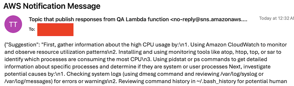
    3. Check SNS email notification delivery.
      AWS SNS notification email showing troubleshooting steps for high CPU usageCode snippet showing CPU usage troubleshooting steps in red text

Best practices and considerations

Monitoring infrastructure requires precise alert prioritization and threshold configuration. Alert aggregation techniques prevent notification overload by consolidating event streams and reducing redundant alerts. Operational teams must maintain dashboards through consistent updates and metric integration, providing real-time visibility into system performance and health.

Security implementations focus on least-privilege AWS Identity and Access Management (IAM) roles, restricting access to critical resources and minimizing potential breach vectors. Data protection strategies involve encryption protocols for information at rest and in transit, using AES-256 standards. Automated security audit processes scan automation scripts, identifying potential vulnerabilities through code analysis and runtime inspection.

Performance optimization in serverless architectures uses Lambda extensions to cache knowledge base content, reducing latency and improving response times. Retry mechanisms for API calls implement exponential backoff strategies, mitigating transient network exceptions and enhancing system resilience. Execution time monitoring of Lambda functions enables detection of anomalies through statistical analysis, providing insights into potential system-wide incidents or performance degradations.

Clean up

To avoid incurring future charges, delete the resources by deleting the parent stack on the AWS CloudFormation console.

Conclusion

This solution provides a robust framework for automated EMR cluster monitoring and incident response. By combining real-time monitoring with AI-powered remediation suggestions and automated execution, organizations can significantly reduce MTTR for common Amazon EMR issues while building a knowledge base for future incident response.

Try out this solution for your own use case, and leave your feedback in the comments section.


About the authors

Author Yu-ting Su, Sr. Hadoop System Engineer, AWS Support Engineering. Yu-Ting is a Sr. Hadoop Systems Engineer at Amazon Web Services (AWS). Her expertise is in Amazon EMR and Amazon OpenSearch Service. She’s passionate about distributing computation and helping people to bring their ideas to life.

Use Databricks Unity Catalog Open APIs for Spark workloads on Amazon EMR

Post Syndicated from Venkat Viswanathan original https://aws.amazon.com/blogs/big-data/use-databricks-unity-catalog-open-apis-for-spark-workloads-on-amazon-emr/

This post was written with John Spencer, Sreeram Thoom, and Dipankar Kushari from Databricks.

Organizations need seamless access to data across multiple platforms and business units. A common scenario involves one team using Amazon EMR for data processing while needing to access data that another team manages in Databricks Unity Catalog. Traditionally, this would require data duplication or complex manual setups.

Although both Amazon EMR and Databricks Unity Catalog are powerful tools on their own, integrating them effectively is crucial for maintaining strong data governance, security, and operational efficiency. In this post, we demonstrate how to achieve this integration using Amazon EMR Serverless, though the approach works well with other Amazon EMR deployment options and Unity Catalog OSS.

EMR Serverless makes running big data analytics frameworks straightforward by offering a serverless option that automatically provisions and manages the infrastructure required to run big data applications. Teams can run Apache Spark and other workloads without the complexity of cluster management, while providing cost-effective scaling based on actual workload demands and seamless integration with AWS services and security controls.

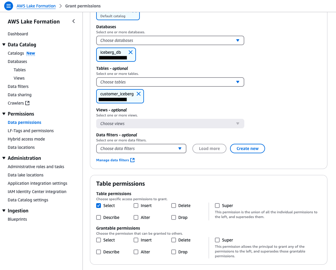
Databricks Unity Catalog serves as a unified governance solution for data and AI assets, providing centralized access control and auditing capabilities. It enables fine-grained permissions across workspaces and cloud platforms, while supporting comprehensive metadata management and data discovery across the organization, and can complement governance tools like AWS Lake Formation.

To enable Amazon EMR to process data maintained in Unity Catalog, the data team traditionally copies data products across the platforms to a location accessible by Amazon EMR. The practice of data duplication not only leads to increased storage costs, but also severely impacts data quality and makes it challenging to effectively enforce same governance policies across different systems, track data lineage, enforce data retention policies, and maintain consistent access controls across the organization.

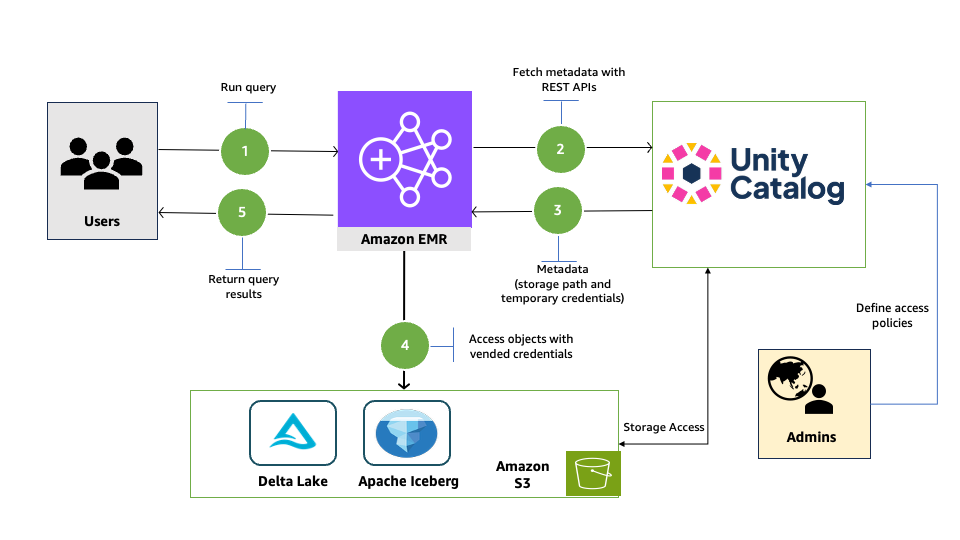
Now using Unity Catalog’s Open REST APIs, Amazon EMR customers can read from and write to Databricks Unity Catalog and Unity Catalog OSS tables using Spark, enabling cross-platform interoperability while maintaining governance and access controls across Amazon EMR and Unity Catalog.

Solution overview

In this post, we will provide an overview of EMR Spark workload integration with Databricks Unity Catalog and walk through the end-to-end process of reading from and writing to Databricks Unity Catalog tables using Amazon EMR and Spark. We show you how to configure EMR Serverless to interact with Databricks Unity Catalog, run an interactive Spark workload to access the data, and run an analysis to derive insights.

The following diagram illustrates the solution architecture.

Prerequisites

You must have the following prerequisites:

In the following sections, we walk through the process of reading and writing to Unity Catalog with EMR Serverless.

Enable Unity Catalog for external access

Log in to your workspace as a Databricks admin and complete the following steps to configure external access to read Databricks objects:

  1. Enable external data access for your metastore. For instructions, see Enable external data access on the metastore.
  2. Set up a principal that will be configured with Amazon EMR for data access.
  3. Grant the principal the privilege to configure the integration of the EXTERNAL USE SCHEMA privilege on the schema containing the objects. For instructions, see Grant a principal EXTERNAL USE SCHEMA.
  4. For this post, we generate a Databricks personal access token (PAT) for the principal and note it down. For instructions, refer to Authorizing access to Databricks resources and Databricks personal access token authentication.

For a production deployment, store the PAT in AWS Secrets Manager. You can use it in a later step to read and write to Unity Catalog with Amazon EMR.

Configure EMR Spark to access Unity Catalog

In this walkthrough, we run PySpark interactive queries through notebooks using EMR Studio. Complete the following steps:

  1. Open the AWS Management Console with administrator permission.
  2. Create an EMR Studio to run interactive workloads. To create a workspace, you need to specify the S3 bucket created in the prerequisites and the minimum service role for EMR Serverless. For instructions, see Set up an EMR Studio.
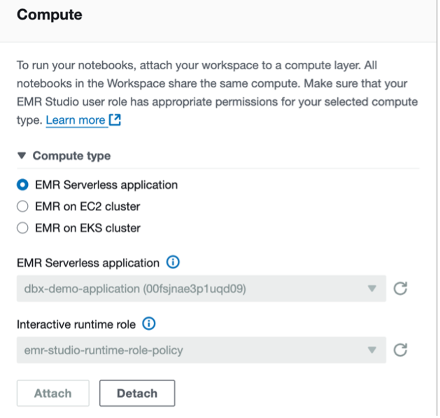
  3. For this post, we create two EMR Serverless applications. For instructions, see Creating an EMR Serverless application from the EMR Studio console.
    1. For Iceberg tables, create an EMR Serverless application called dbx-demo-application-iceberg with version 7.8.0 or higher. Make sure to deselect Use AWS Glue Data Catalog as Metastore under Additional Configurations, Metastore configuration. Add the following Spark configuration (see Configure applications). Provide the name of the catalog in Unity Catalog that contains your tables and the URL of the Databricks workspace.
      {
          "runtimeConfiguration": [
              {
                  "classification": "spark-defaults",
                  "properties": {
                      "spark.jars": "/usr/share/aws/iceberg/lib/iceberg-spark3-runtime.jar",
                      "spark.jars.packages": "io.unitycatalog:unitycatalog-spark_2.12:0.2.0",
                      "spark.sql.extensions": "org.apache.iceberg.spark.extensions.IcebergSparkSessionExtensions",
                      "spark.sql.defaultCatalog": "<uc-catalog-name>",
                      "spark.sql.catalog.<uc-catalog-name>": "org.apache.iceberg.spark.SparkCatalog",
                      "spark.sql.catalog.<uc-catalog-name>.uri": "https://<workspace-url>/api/2.1/unity-catalog/iceberg-rest",
                      "spark.sql.catalog.<uc-catalog-name>.type": "rest",
                      "spark.sql.catalog.<uc-catalog-name>.warehouse": "<uc-catalog-name>"
                  }
              }
          ]
      }

    2. For Delta tables, create an EMR Serverless application called dbx-demo-application and version 7.8.0 or higher. Make sure to deselect Use AWS Glue Data Catalog as Metastore under Additional Configurations, Metastore configuration. Add the following Spark configuration (see Configure applications). Provide the name of the catalog in Unity Catalog that contains your tables and the URL of the Databricks workspace.
      {
          "runtimeConfiguration": [
              {
                  "classification": "spark-defaults",
                  "properties": {
                      "spark.jars": "/usr/share/aws/delta/lib/delta-spark.jar,/usr/share/aws/delta/lib/delta- storage.jar",
                      "spark.jars.packages": "io.unitycatalog:unitycatalog-spark_2.12:0.2.0",
                      "spark.sql.extensions": "io.delta.sql.DeltaSparkSessionExtension",
                      "spark.sql.defaultCatalog": "<uc-catalog-name>",
                      "spark.sql.catalog.spark_catalog": "io.unitycatalog.spark.UCSingleCatalog",
                      "spark.sql.catalog.<uc-catalog-name>": "io.unitycatalog.spark.UCSingleCatalog",
                      "spark.sql.catalog.<uc-catalog-name>.uri": "https://<workspace-url>/api/2.1/unity-catalog"
                  }
              }
          ]
      }

  4. To set up your interactive workload with a runtime role, see Run interactive workloads with EMR Serverless through EMR Studio.

Read and write to Unity Catalog with Amazon EMR

Launch the workspace created in the previous step. Download the notebooks create-delta-table and create-iceberg-table and upload them to the EMR Studio workspace.

The create-delta-table.ipynb notebook configures the metastore properties to work with Delta tables. The create-iceberg-table.ipynb notebook configures the metastore properties to work with Iceberg tables.

Add the generated token to the session.

For a production deployment, store the PAT in Secrets Manager.

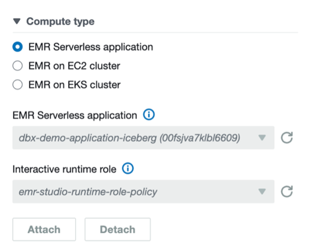
For Iceberg tables, connect to the EMR Serverless application dbx-demo-application-iceberg with the runtime role created in earlier steps under compute and run the notebook (create-iceberg-table). Select PySpark as the kernel and execute each cell in the notebook by choosing the run icon. Refer to Submit a job run or interactive workload for further details about how to run an interactive notebook.

We use the following code to create an external Iceberg table in the catalog:

CREATE SCHEMA IF NOT EXISTS customerschema;
USE SCHEMA customerschema;
CREATE TABLE IF NOT EXISTS iceberg_customer (id string, name string, country string) USING iceberg; 
insert into iceberg customer values('1','Alice','US');

For Delta tables, connect to the EMR Serverless application dbx-demo-application with the runtime role created in earlier steps and run the notebook (create-delta-table). Select PySpark as the kernel and execute each cell in the notebook by choosing the run icon. Refer to Submit a job run or interactive workload for further details about how to run an interactive notebook.

We use the following code to create an external Delta table in the catalog:

CREATE SCHEMA IF NOT EXISTS customerschema;
USE SCHEMA customerschema;
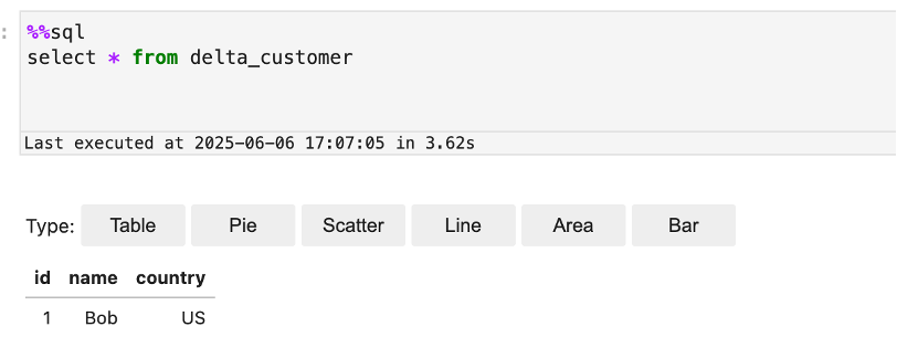
CREATE TABLE IF NOT EXISTS delta_customer (id int, name string, country string) USING delta LOCATION ‘s3://<bucket_name>/emr-dbx/external/customerschema/delta_customer’;
insert into delta_customer values(1,'Bob','US'); 

Verify in Databricks for both Iceberg and Delta tables

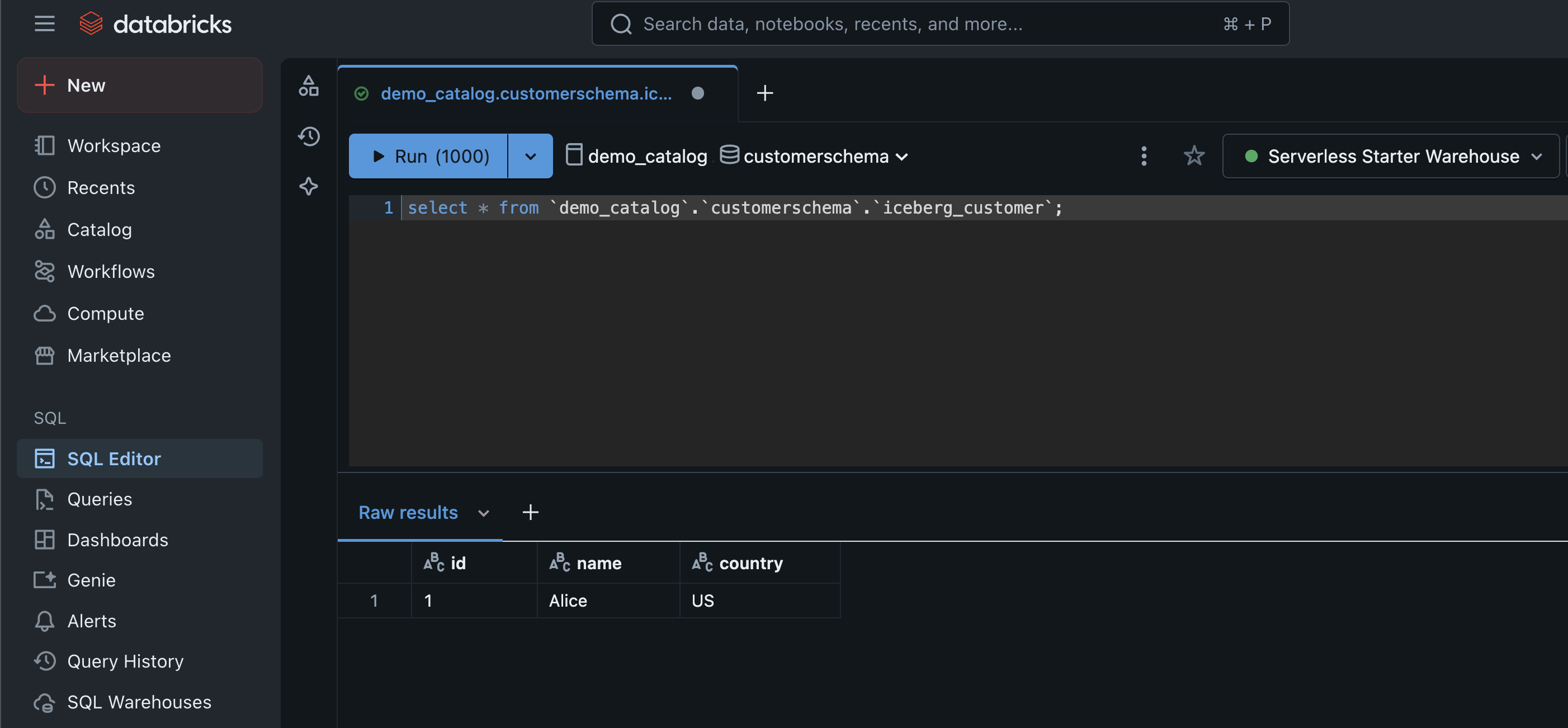
Now you can run queries in Databricks Unity Catalog to show the records inserted into the Iceberg and Delta tables from EMR Serverless:

  1. Log in to your Databricks workspace.
  2. Choose SQL Editor in the navigation pane.
  3. Run queries for both Iceberg and Delta tables.
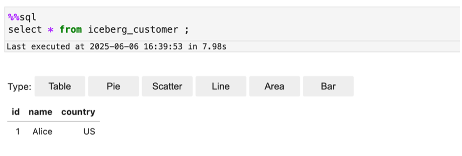
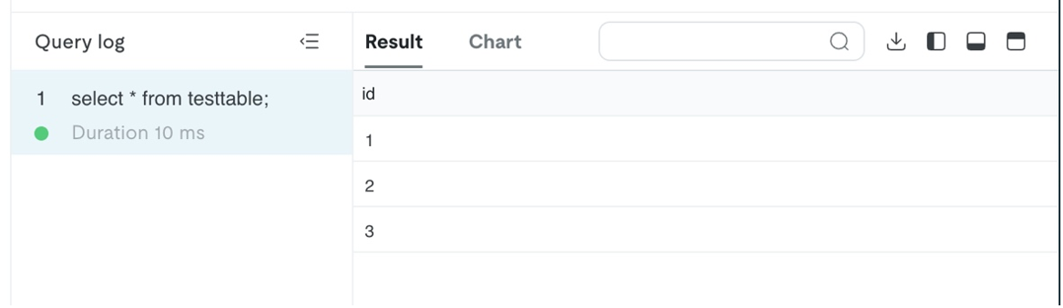
  4. Verify the results show the same as what you saw in the Jupyter notebook in EMR Studio.

The following screenshot shows an example of querying the Iceberg table.

The following screenshot shows an example of querying the Delta table.

Clean up

Clean up the resources used in this post to avoid additional charges:

  1. Delete the IAM roles for this post.
  2. Delete the EMR applications and EMR Studio setup created for this post.
  3. Delete the resources created in Unity Catalog.
  4. Empty and then delete the S3 bucket.

Summary

In this post, we demonstrated the powerful interoperability between Amazon EMR and Databricks Unity Catalog by walking through how to enable external access to Unity Catalog, configure EMR Spark to connect seamlessly with Unity Catalog, and perform DML and DDL operations on Unity Catalog tables using EMR Serverless.

To learn more about using EMR Serverless, see Getting started with Amazon EMR Serverless. To learn more about using tools like EMR Spark with Unity Catalog, see Unity Catalog integrations.


About the authors

Venkatavaradhan (Venkat) Viswanathan is a Global Partner Solutions Architect at Amazon Web Services. Venkat is a Technology Strategy Leader in Data, AI, ML, generative AI, and Advanced Analytics. Venkat is a Global SME for Databricks and helps AWS customers design, build, secure, and optimize Databricks workloads on AWS.

Srividya Parthasarathy is a Senior Big Data Architect on the AWS Lake Formation team. She works with the product team and customers to build robust features and solutions for their analytical data platform. She enjoys building data mesh solutions and sharing them with the community.

Ramkumar Nottath is a Principal Solutions Architect at AWS focusing on Analytics services. He enjoys working with various customers to help them build scalable, reliable big data and analytics solutions. His interests extend to various technologies such as analytics, data warehousing, streaming, data governance, and machine learning. He loves spending time with his family and friends.

John Spencer is a Product Manager at Databricks, dedicated to making Unity Catalog work seamlessly with customers’ ecosystems of tools and platforms so they can easily access, govern, and use their data.

Sreeram Thoom is a Specialist Solutions Architect at Databricks helping customers design secure, scalable applications on the Data Lakehouse.

Dipankar Kushari is a specialist solutions architect at Databricks helping customer architect and build secured applications on Data Lakehouse.

RocksDB 101: Optimizing stateful streaming in Apache Spark with Amazon EMR and AWS Glue

Post Syndicated from Melody Yang original https://aws.amazon.com/blogs/big-data/rocksdb-101-optimizing-stateful-streaming-in-apache-spark-with-amazon-emr-and-aws-glue/

Real-time streaming data processing is a strategic imperative that directly impacts business competitiveness. Organizations face mounting pressure to process massive data streams instantaneously—from detecting fraudulent transactions and delivering personalized customer experiences to optimizing complex supply chains and responding to market dynamics milliseconds ahead of competitors.

Apache Spark Structured Streaming addresses these critical business challenges through its stateful processing capabilities, enabling applications to maintain and update intermediate results across multiple data streams or time windows. RocksDB was introduced in Apache Spark 3.2, offering a more efficient alternative to the default HDFS-based in-memory store. RocksDB excels in stateful streaming in scenarios that require handling large quantities of state data. It delivers optimal performance benefits, particularly in reducing Java virtual machine (JVM) memory pressure and garbage collection (GC) overhead.

This post explores RocksDB’s key features and demonstrates its implementation using Spark on Amazon EMR and AWS Glue, providing you with the knowledge you need to scale your real-time data processing capabilities.

RocksDB state store overview

Spark Structured Streaming processes fall into two categories:

  • Stateful: Requires tracking intermediate results across micro-batches (for example, when running aggregations and de-duplication).
  • Stateless: Processes each batch independently.

A state store is required by stateful applications that track intermediate query results. This is essential for computations that depend on continuous events and change results based on each batch of input, or on aggregate data over time, including late arriving data. By default, Spark offers a state store that keeps states in JVM memory, which is performant and sufficient for most general streaming cases. However, if you have a large number of stateful operations in a streaming application—such as, streaming aggregation, streaming dropDuplicates, stream-stream joins, and so on—the default in-memory state store might face out-of-memory (OOM) issues because of a large JVM memory footprint or frequent GC pauses, resulting in degraded performance.

Advantages of RocksDB over in-memory state store

RocksDB addresses the challenges of an in-memory state store through off-heap memory management and efficient checkpointing.

  • Off-heap memory management: RocksDB stores state data in OS-managed off-heap memory, reducing GC pressure. While off-heap memory still consumes machine memory, it doesn’t occupy space in the JVM. Instead, its core memory structures, such as block cache or memTables, allocate directly from the operating system, bypassing the JVM heap. This approach makes RocksDB an optimal choice for memory-intensive applications.
  • Efficient checkpointing: RocksDB automatically saves state changes to checkpoint locations, such as Amazon Simple Storage Service (Amazon S3) paths or local directories, helping to ensure full fault tolerance. When interacting with S3, RocksDB is designed to improve checkpointing efficiency; it does this through incremental updates and compaction to reduce the amount of data transferred to S3 during checkpoints, and by persisting fewer large state files compared to the many small files of the default state store, reducing S3 API calls and latency.

Implementation considerations

RocksDB operates as a native C++ library embedded within the Spark executor, using off-heap memory. While it doesn’t fall under JVM GC control, it still affects overall executor memory usage from the YARN or OS perspective. RocksDB’s off-heap memory usage might exceed YARN container limits without triggering container termination, potentially leading to OOM issues. You should consider the following approaches to manage Spark’s memory:

Adjust the Spark executor memory size

Increase spark.executor.memoryOverheadorspark.executor.memoryOverheadFactor to leave more room for off-heap usage. The following example sets half (4 GB) of spark.executor.memory (8 GB) as the memory overhead size.

# Total executor memory = 8GB (heap) + 4GB (overhead) = 12GB
spark-submit \
. . . . . . . .
--conf spark.executor.memory=8g \         # JVM Heap
--conf spark.executor.memoryOverhead=4g \ # Off-heap allocation (RocksDB + other native)
. . . . . . . .

For Amazon EMR on Amazon Elastic Compute Cloud (Amazon EC2), enabling YARN memory control with the following strict container memory enforcement through polling method preempts containers to avoid node-wide OOM failures:

yarn.nodemanager.resource.memory.enforced = false
yarn.nodemanager.elastic-memory-control.enabled = false
yarn.nodemanager.pmem-check-enabled = true 
or 
yarn.nodemanager.vmem-check-enabled = true

Off-heap memory control

Use RocksDB-specific settings to configure memory usage. More details can be found in the Best practices and considerations section.

Get started with RocksDB on Amazon EMR and AWS Glue

To turn on the state store RocksDB in Spark, configure your application with the following setting:

spark.sql.streaming.stateStore.providerClass=org.apache.spark.sql.execution.streaming.state.RocksDBStateStoreProvider

In the following sections, we explore creating a sample Spark Structured Streaming job with RocksDB enabled running on Amazon EMR and AWS Glue respectively.

RocksDB on Amazon EMR

Amazon EMR versions 6.6.0 and later support RocksDB, including Amazon EMR on EC2, Amazon EMR serverless and Amazon EMR on Amazon Elastic Kubernetes Service (Amazon EKS). In this case, we use Amazon EMR on EC2 as an example.

Use the following steps to run a sample streaming job with RocksDB enabled.

  1. Upload the following sample script to s3://<YOUR_S3_BUCKET>/script/sample_script.py
from pyspark.sql import SparkSession
from pyspark.sql.functions import explode, split, col, expr
import random

# List of words
words = ["apple", "banana", "orange", "grape", "melon", 
         "peach", "berry", "mango", "kiwi", "lemon"]

# Create random strings from words
def generate_random_string():
    return " ".join(random.choices(words, k=5)) 
    
    
# Create Spark Session
spark = SparkSession \
    .builder \
    .appName("StreamingWordCount") \
    .config("spark.sql.streaming.stateStore.providerClass","org.apache.spark.sql.execution.streaming.state.RocksDBStateStoreProvider") \
    .getOrCreate()


# Register UDF
spark.udf.register("random_string", generate_random_string)

# Create streaming data
raw_stream = spark.readStream \
    .format("rate") \
    .option("rowsPerSecond", 1) \
    .load() \
    .withColumn("words", expr("random_string()"))

# Execute word counts
wordCounts = raw_stream.select(explode(split(raw_stream.words, " ")).alias("word")).groupby("word").count()

# Output the results
query = wordCounts \
    .writeStream \
    .outputMode("complete") \
    .format("console") \
    .start()

query.awaitTermination()
  1. On the AWS Management Console for Amazon EMR, choose Create Cluster
  2. For Name and applications – required, select the latest Amazon EMR release.
  3. For Steps, choose Add. For Type, select Spark application.
  4. For Name, enter GettingStartedWithRocksDB and s3://<YOUR_S3_BUCKET>/script/sample_script.py as the Application location.
  5. Choose Save step.
  6. For other settings, choose the appropriate settings based on your use case.
  7. Choose Create cluster to start the streaming application via Amazon EMR step.

RocksDB on AWS Glue

AWS Glue 4.0 and later versions support RocksDB. Use the following steps to run the sample job with RocksDB enabled on AWS Glue.

  1. On the AWS Glue console, in the navigation pane, choose ETL jobs.
  2. Choose Script editor and Create script.
  3. For the job name, enter GettingStartedWithRocksDB.
  4. Copy the script from the previous example and paste it on the Script tab.
  5. On Job details tab, for Type, select Spark Streaming.
  6. Choose Save, and then choose Run to start the streaming job on AWS Glue.

Walkthrough details

Let’s dive deep into the script to understand how to run a simple stateful Spark application with RocksDB using the following example pySpark code.

  1. First, set up RocksDB as your state store by configuring the provider class:
spark = SparkSession \
    .builder \
    .appName("StreamingWordCount") \
    .config("spark.sql.streaming.stateStore.providerClass","org.apache.spark.sql.execution.streaming.state.RocksDBStateStoreProvider") \
    .getOrCreate()
  1. To simulate streaming data, create a data stream using the rate source type. It generates one record per second, containing five random fruit names from a pre-defined list.
# List of words
words = ["apple", "banana", "orange", "grape", "melon", 
         "peach", "berry", "mango", "kiwi", "lemon"]

# Create random strings from words
def generate_random_string():
    return " ".join(random.choices(words, k=5))
# Register UDF
spark.udf.register("random_string", generate_random_string)

# Create streaming data
raw_stream = spark.readStream \
    .format("rate") \
    .option("rowsPerSecond", 1) \
    .load() \
    .withColumn("words", expr("random_string()"))
  1. Create a word counting operation on the incoming stream. This is a stateful operation because it maintains running counts between processing intervals, that is, previous counts must be stored to calculate the next new totals.
# Split raw_stream into words and counts them
wordCounts = raw_stream.select(explode(split(raw_stream.words, " ")).alias("word")).groupby("word").count()
  1. Finally, output the word count totals to the console:
# Output the results
query = wordCounts \
    .writeStream \
    .outputMode("complete") \
    .format("console") \
    .start()

Input data

In the same sample code, test data (raw_stream) is generated at a rate of one-row-per-second, as shown in the following example:

+-----------------------+-----+--------------------------------+
|timestamp              |value|words                           |
+-----------------------+-----+--------------------------------+
|2025-04-18 07:05:57.204|125  |berry peach orange banana banana|
+-----------------------+-----+--------------------------------+

Output result

The streaming job produces the following results in the output logs. It demonstrates how Spark Structured Streaming maintains and updates the state across multiple micro-batches:

  • Batch 0: Starts with an empty state
  • Batch 1: Processes multiple input records, resulting in initial counts for every one of the 10 fruits (for example, banana appears 8 times)
  • Batch 2: Running totals based on new occurrences from the next set of records are added to the counts (for example,  banana increases from 8 to 15, indicating 7 new occurrences).

-------------------------------------------
Batch: 0
-------------------------------------------
+----+-----+
|word|count|
+----+-----+
+----+-----+

-------------------------------------------
Batch: 1
-------------------------------------------
+------+-----+
|  word|count|
+------+-----+
|banana|    8|
|orange|    4|
| apple|    3|
| berry|    5|
| lemon|    7|
|  kiwi|    6|
| melon|    8|
| peach|    8|
| mango|    7|
| grape|    9|
+------+-----+

-------------------------------------------
Batch: 2
-------------------------------------------
+------+-----+
|  word|count|
+------+-----+
|banana|   15|
|orange|    8|
| apple|    7|
| berry|   11|
| lemon|   12|
|  kiwi|   11|
| melon|   16|
| peach|   15|
| mango|   12|
| grape|   13|
+------+-----+

State store logs

RocksDB generates detailed logs during the job run, like the following:

INFO    2025-04-18T07:52:28,378 83933   org.apache.spark.sql.execution.streaming.MicroBatchExecution    [stream execution thread for [id = xxxxxxxx-xxxx-xxxx-xxxx-xxxxxxxxxxxx, runId = xxxxxxxx-xxxx-xxxx-xxxx-xxxxxxxxxxxx]] 60  Streaming query made progress: {
  "id": "xxxxxxxx-xxxx-xxxx-xxxx-xxxxxxxxxxxx",
  "runId": "xxxxxxxx-xxxx-xxxx-xxxx-xxxxxxxxxxxx",
  "name": null,
  "timestamp": "2025-04-18T07:52:27.642Z",
  "batchId": 39,
  "numInputRows": 1,
  "inputRowsPerSecond": 100.0,
  "processedRowsPerSecond": 1.3623978201634879,
  "durationMs": {
    "addBatch": 648,
    "commitOffsets": 39,
    "getBatch": 0,
    "latestOffset": 0,
    "queryPlanning": 10,
    "triggerExecution": 734,
    "walCommit": 35
  },
  "stateOperators": [
    {
      "operatorName": "stateStoreSave",
      "numRowsTotal": 10,
      "numRowsUpdated": 4,
      "allUpdatesTimeMs": 18,
      "numRowsRemoved": 0,
      "allRemovalsTimeMs": 0,
      "commitTimeMs": 3629,
      "memoryUsedBytes": 174179,
      "numRowsDroppedByWatermark": 0,
      "numShufflePartitions": 36,
      "numStateStoreInstances": 36,
      "customMetrics": {
        "rocksdbBytesCopied": 5009,
        "rocksdbCommitCheckpointLatency": 533,
        "rocksdbCommitCompactLatency": 0,
        "rocksdbCommitFileSyncLatencyMs": 2991,
        "rocksdbCommitFlushLatency": 44,
        "rocksdbCommitPauseLatency": 0,
        "rocksdbCommitWriteBatchLatency": 0,
        "rocksdbFilesCopied": 4,
        "rocksdbFilesReused": 24,
        "rocksdbGetCount": 8,
        "rocksdbGetLatency": 0,
        "rocksdbPinnedBlocksMemoryUsage": 3168,
        "rocksdbPutCount": 4,
        "rocksdbPutLatency": 0,
        "rocksdbReadBlockCacheHitCount": 8,
        "rocksdbReadBlockCacheMissCount": 0,
        "rocksdbSstFileSize": 35035,
        "rocksdbTotalBytesRead": 136,
        "rocksdbTotalBytesReadByCompaction": 0,
        "rocksdbTotalBytesReadThroughIterator": 0,
        "rocksdbTotalBytesWritten": 228,
        "rocksdbTotalBytesWrittenByCompaction": 0,
        "rocksdbTotalBytesWrittenByFlush": 5653,
        "rocksdbTotalCompactionLatencyMs": 0,
        "rocksdbWriterStallLatencyMs": 0,
        "rocksdbZipFileBytesUncompressed": 266452
      }
    }
  ],
  "sources": [
    {
      "description": "RateStreamV2[rowsPerSecond=1, rampUpTimeSeconds=0, numPartitions=default",
      "startOffset": 63,
      "endOffset": 64,
      "latestOffset": 64,
      "numInputRows": 1,
      "inputRowsPerSecond": 100.0,
      "processedRowsPerSecond": 1.3623978201634879
    }
  ],
  "sink": {
    "description": "org.apache.spark.sql.execution.streaming.ConsoleTable$@2cf39784",
    "numOutputRows": 10
  }
}

In Amazon EMR on EC2, these logs are available on the node where the YARN ApplicationMaster container is running. They can be found at/var/log/hadoop-yarn/containers/<Application ID>/<container_id>/stderr.

As for AWS Glue, you can find the RocksDB metrics in Amazon CloudWatch, under the log group /aws-glue/jobs/error.

RocksDB metrics

The metrics from the preceding logs provide insights on RocksDB status. The followings are some example metrics you might find useful when investigating streaming job issues:

  • rocksdbCommitCheckpointLatency: Time spent writing checkpoints to local storage
  • rocksdbCommitCompactLatency: Duration of checkpoint compaction operations during checkpoint commits
  • rocksdbSstFileSize: Current size of SST files in RocksDB.

Deep dive into RocksDB key concepts

To better understand the state metrics shown in the logs, we deep dive into RocksDB’s key concepts: MemTable, sorted string table (SST) file, and checkpoints. Additionally, we provide some tips for best practices and fine-tuning.

High level architecture

RocksDB is a local, non-distributed persistent key-value store embedded in Spark executors. It enables scalable state management for streaming workloads, backed by Spark’s checkpointing for fault tolerance. As shown in the preceding figure, RocksDB stores data in memory and also on disk. RocksDB’s ability to spill data over to disk is what allows Spark Structured Streaming to handle state data that exceeds the available memory.

Memory:

  • Write buffers (MemTables): Designated memory to buffer writes before flushing onto disk
  • Block cache (read buffer): Reduces query time by caching results from disk

Disk:

  • SST files: Sorted String Table saved as SST file format for fast access

MemTable: Stored off-heap

MemTable, shown in the preceding figure, is an in-memory store where data is first written off-heap, before being flushed to disk as an SST file. RocksDB caches the latest two batches of data (hot data) in MemTable to reduce streaming process latency. By default, RocksDB only has two MemTables—one is active and the other is read-only. If you have sufficient memory, the configuration spark.sql.streaming.stateStore.rocksdb.maxWriteBufferNumber can be increased to have more than two MemTables. Among these MemTables, there is always one active table, and the rest are read-only MemTables used as write buffers.

SST files: Stored on Spark executor’s local disk

SST files are block-based tables stored on the Spark executor’s local disk. When the in-memory state data can no longer fit into a MemTable (defined by a Spark configuration writeBufferSizeMB), the active table is marked as immutable, saving it as the SST file format, which switches it to a read-only MemTable while asynchronously flushing it to local disks. While flushing, the immutable MemTable can still be read, so that the most recent state data is available with minimal read latency.

Reading from RocksDB follows the sequence demonstrated by the preceding diagram:

  1. Read from the active MemTable.
  2. If not found, iterate through read-only MemTables in the order of newest to oldest.
  3. If not found, read from BlockCache (read buffer).
  4. If misses, load index (one index per SST) from disk into BlockCache. Look up key from index and if hits, load data block onto BlockCache and return result.

SST files are stored on executors’ local directories under the path of spark.local.dir (default: /tmp) or yarn.nodemanager.local-dirs:

  • Amazon EMR on EC2 – ${yarn.nodemanager.local-dirs}/usercache/hadoop/appcache/<yarn_app_id>/<spark_app_id>/
  • Amazon EMR Serverless, Amazon EMR on EKS, AWS Glue${spark.local.dir}/<spark_app_id>/

Additionally, by using application logs, you can track the MemTable flush and SST file upload status under the file path:

  • Amazon EMR on EC2/var/log/hadoop-yarn/containers/<application_id>/<container_id>/stderr
  • Amazon EMR on EKS –/var/log/spark/user/<spark_app_name>-<spark_executor_ID>/stderr

The following is an example command to check the SST file status in an executor log from Amazon EMR on EKS:

cat /var/log/spark/user/<spark_app_name>-<spark_executor_ID>/stderr/current | grep old

or

kubectl logs <spark_executor_pod_name> --namespace emr -c spark-kubernetes-executor | grep old

The following screenshot is an example of the output of either command.

You can use the following examples to check if the MemTable records were deleted and flushed out to SST:

cat /var/log/spark/user/<spark_app_name>-<spark_executor_ID>/stderr/current | grep deletes

or

kubectl logs <spark_executor_pod_name> --namespace emr -c spark-kubernetes-executor | grep deletes

The following screenshot is an example of the output of either command.

Checkpoints: Stored on the executor’s local disk or in an S3 bucket

To handle fault tolerance and fail over from the last committed point, RocksDB supports checkpoints. The checkpoint files are usually stored on the executor’s disk or in an S3 bucket, including snapshot and delta or changelog data files.

Starting with Amazon EMR 7.0 and AWS Glue5.0, RocksDB state store provides a new feature called changelog checkpointing to enhance checkpoint performance. when the changelog is enabled (disabled by default) using the setting spark.sql.streaming.stateStore.rocksdb.changelogCheckpointing.enabled, RocksDB writes smaller change logs to the storage location (the local disk by default) instead of frequently persisting large snapshot data. Note that snapshots are still created but less frequently, as shown in the following screenshot.

Here’s an example of a checkpoint location path when overridden to an S3 bucket: s3://<S3BUCKET>/<checkpointDir>/state/0/spark_parition_ID/state_version_ID.zip

Best practices and considerations

This section outlines key strategies for fine-tuning RocksDB performance and avoiding common pitfalls.

1. Memory management for RocksDB

To prevent OOM errors on Spark executors, you can configure RocksDB’s memory usage at either the node level or instance level:

  • Node level (recommended): Enforce a global off-heap memory limit per executor. In this context, each executor is treated as a RocksDB node. If an executor processes N partitions of a stateful operator, it will have N number of RocksDB instances on a single executor.
  • Instance-level: Fine-tune individual RocksDB instances.

Node-level memory control per executor

Starting with Amazon EMR 7.0 and AWS Glue 5.0 (Spark 3.5), a critical Spark configuration, boundedMemoryUsage, was introduced (through SPARK-43311) to enforce a global memory cap at a single executor level that is shared by multiple RocksDB instances. This prevents RocksDB from consuming unbounded off-heap memory, which could lead to OOM errors or executor termination by resource managers such as YARN or Kubernetes.

The following example shows the node-level configuration:

 # Bound total memory usage per executor 
 "spark.sql.streaming.stateStore.rocksdb.boundedMemoryUsage": "true"
 # Set a static total memory size per executor
 "spark.sql.streaming.stateStore.rocksdb.maxMemoryUsageMB": "500"
 # For read-heavy workloads, split memory allocation between write buffers (30%) and block cache (70%) 
 "spark.sql.streaming.stateStore.rocksdb.writeBufferCacheRatio": "0.3"

A single RocksDB instance level control

For granular memory management, you can configure individual RocksDB instances using the following settings:

# Control MemTable (write buffer) size and count
"spark.sql.streaming.stateStore.rocksdb.writeBufferSizeMB": "64"
"spark.sql.streaming.stateStore.rocksdb.maxWriteBufferNumber": "4"
  • writeBufferSizeMB (default: 64, suggested: 64 – 128): Controls the maximum size of a single MemTable in RocksDB, affecting memory usage and write throughput. This setting is available in Spark3.5 – [SPARK-42819] and later. It determines the size of the memory buffer before state data is flushed to disk. Larger buffer sizes can improve write performance by reducing SST flush frequency but will increase the executor’s memory usage. Adjusting this parameter is crucial for optimizing memory usage and write throughput.
  • maxWriteBufferNumber (default: 2, suggested: 3 – 4): Sets the total number of active and immutable MemTables.

For read-heavy workloads, prioritize the following block cache tuning over write buffers to reduce disk I/O. You can configure SST block size and caching as follows:

"spark.sql.streaming.stateStore.rocksdb.blockSizeKB": "64"
"spark.sql.streaming.stateStore.rocksdb.blockCacheSizeMB": "128"
  •  blockSizeKB (default: 4, suggested: 64–128): When an active MemTable is full, it becomes a read-only memTable. From there, new writes continue to accumulate in a new table. The read-only MemTable is flushed into SST files on the disk. The data in SST files is approximately chunked into fixed-sized blocks (default is 4 KB). Each block, in turn, keeps multiple data entries. When writing data to SST files, you can compress or encode data efficiently within a block, which often results in a smaller data size compared with its raw format.

For workloads with a small state size (such as less than 10 GB), the default block size is usually sufficient. For a large state (such as more than 50 GB), increasing the block size can improve compression efficiency and sequential read performance but increase CPU overhead.

  • blockCacheSizeMB (default: 8, suggested: 64–512, large state: more than 1024): When retrieving data from SST files, RocksDB provides a cache layer (block cache) to improve the read performance. It first locates the data block where the target record might reside, then caches the block to memory, and finally searches that record within the cached block. To avoid frequent reads of the same block, the block cache can be used to keep the loaded blocks in memory.

2. Clean up state data at checkpoint

To help ensure that your state file sizes and storage costs remain under control when checkpoint performance becomes a concern, use the following Spark configurations to adjust cleanup frequency, retention limits, and checkpoint file types:

# clean up RocksDB state every 30 seconds
"spark.sql.streaming.stateStore.maintenanceInterval":"30s"
# retain only the last 50 state versions  
"spark.sql.streaming.minBatchesToRetain":"50"
# use changelog instead of snapshots
"spark.sql.streaming.stateStore.rocksdb.changelogCheckpointing.enabled":"true"
  • maintenanceInterval (default: 60 seconds): Retaining a state for a long period of time can help reduce maintenance cost and background IO. However, longer intervals increase file listing time, because state stores often scan every retained file.
  • minBatchesToRetain (default: 100, suggested: 10–50): Limits the number of state versions retained at checkpoint locations. Reducing this number results in fewer files being persisted and reduces storage usage.
  • changelogCheckpointing (default: false, suggested: true): Traditionally, RocksDB snapshots and uploads incremental SST files to checkpoint. To avoid this cost, changelog checkpointing was introduced in Amazon EMR7.0+ and AWS Glue 5.0, which write only state changes since the last checkpoint.

To track an SST file’s retention status, you can search RocksDBFileManager entries in the executor logs. Consider the following logs in Amazon EMR on EKS as an example. The output (shown in the screenshot) shows that four SST files under version 102 were uploaded to an S3 checkpoint location, and that an old changelog state file with version 97 was cleaned up.

cat /var/log/spark/user/<spark_app_name>-<spark_executor_ID>/stderr/ current | grep RocksDBFileManager

or

kubectl logs <spark_executor_pod_name> -n emr -c spark-kubernetes-executor | grep RocksDBFileManager

3. Optimize local disk usage

RocksDB consumes local disk space when generating SST files at each Spark executor. While disk usage doesn’t scale linearly, RocksDB can accumulate storage over time based on state data size. When running streaming jobs, if local available disk space gets insufficient, No space left on device errors can occur.

To optimize disk usage by RocksDB, adjust the following Spark configurations:

# compact state files during commit (default:false)
"spark.sql.streaming.stateStore.rocksdb.compactOnCommit": "true"
# number of delta SST files before becomes a consolidated snapshot file(default:10)
"spark.sql.streaming.stateStore.minDeltasForSnapshot": "5" 

Infrastructure adjustments can further mitigate the disk issue:

For Amazon EMR:

For AWS Glue:

  • Use AWS Glue G.2X or larger worker types to avoid the limited disk capacity of G.1X workers.
  • Schedule regular maintenance windows at optimal timing to free up disk space based on workload needs.

Conclusion

In this post, we explored RocksDB as the new state store implementation in Apache Spark Structured Streaming, available on Amazon EMR and AWS Glue. RocksDB offers advantages over the default HDFS-backed in-memory state store, particularly for applications dealing with large-scale stateful operations. RocksDB helps prevent JVM memory pressure and garbage collection issues common with the default state store.

The implementation is straightforward, requiring minimal configuration changes, though you should pay careful attention to memory and disk space management for optimal performance. While RocksDB is not guaranteed to reduce job latency, it provides a robust solution for handling large-scale stateful operations in Spark Structured Streaming applications.

We encourage you to evaluate RocksDB for your use cases, particularly if you’re experiencing memory pressure issues with the default state store or need to handle large amounts of state data in your streaming applications.


About the authors

Melody Yang is a Senior Big Data Solution Architect for Amazon EMR at AWS. She is an experienced analytics leader working with AWS customers to provide best practice guidance and technical advice in order to assist their success in data transformation. Her areas of interests are open-source frameworks and automation, data engineering and DataOps.

Dai Ozaki is a Cloud Support Engineer on the AWS Big Data Support team. He is passionate about helping customers build data lakes using ETL workloads. In his spare time, he enjoys playing table tennis.

Noritaka Sekiyama is a Principal Big Data Architect with Amazon Web Services (AWS) Analytics services. He’s responsible for building software artifacts to help customers. In his spare time, he enjoys cycling on his road bike.

Amir Shenavandeh is a Sr Analytics Specialist Solutions Architect and Amazon EMR subject matter expert at Amazon Web Services. He helps customers with architectural guidance and optimisation. He leverages his experience to help people bring their ideas to life, focusing on distributed processing and big data architectures.

Xi Yang is a Senior Hadoop System Engineer and Amazon EMR subject matter expert at Amazon Web Services. He is passionate about helping customers resolve challenging issues in the Big Data area.

Using AWS Glue Data Catalog views with Apache Spark in EMR Serverless and Glue 5.0

Post Syndicated from Aarthi Srinivasan original https://aws.amazon.com/blogs/big-data/using-aws-glue-data-catalog-views-with-apache-spark-in-emr-serverless-and-glue-5-0/

The AWS Glue Data Catalog has expanded its Data Catalog views feature, and now supports Apache Spark environments in addition to Amazon Athena and Amazon Redshift. This enhancement, launched in March 2025, now makes it possible to create, share, and query multi-engine SQL views across Amazon EMR Serverless, Amazon EMR on Amazon EKS, and AWS Glue 5.0 Spark, as well as Athena and Amazon Redshift Spectrum. The multi-dialect views empower data teams to create SQL views one time and query them through supported engines—whether it’s Athena for ad-hoc analytics, Amazon Redshift for data warehousing, or Spark for large-scale data processing. This cross-engine compatibility means data engineers can focus on building data products rather than managing multiple view definitions or complex permission schemes. Using AWS Lake Formation permissions, organizations can share these views within the same AWS account, across different AWS accounts, and with AWS IAM Identity Center users and groups, without granting direct access to the underlying tables. Features of Lake Formation such as fine-grained access control (FGAC) using Lake Formation-tag based access control (LF-TBAC) can be applied to Data Catalog views, enabling scalable sharing and access control across organizations.

In an earlier blog post, we demonstrated the creation of Data Catalog views using Athena, adding a SQL dialect for Amazon Redshift, and querying the view using Athena and Amazon Redshift. In this post, we guide you through the process of creating a Data Catalog view using EMR Serverless, adding the SQL dialect to the view for Athena, sharing it with another account using LF-Tags, and then querying the view in the recipient account using a separate EMR Serverless workspace and AWS Glue 5.0 Spark job and Athena. This demonstration showcases the versatility and cross-account capabilities of Data Catalog views and access through various AWS analytics services.

Benefits of Data Catalog views

The following are key benefits of Data Catalog views for business solutions:

  • Targeted data sharing and access control – Data Catalog views, combined with the sharing capabilities of Lake Formation, enable organizations to provide specific data subsets to different teams or departments without duplicating data. For example, a retail company can create views that show sales data to regional managers while restricting access to sensitive customer information. By applying LF-TBAC to these views, companies can efficiently manage data access across large, complex organizational structures, maintaining compliance with data governance policies while promoting data-driven decision-making.
  • Multi-service analytics integration – The ability to create a view in one analytics service and query it across Athena, Amazon Redshift, EMR Serverless, and AWS Glue 5.0 Spark breaks down data silos and promotes a unified analytics approach. This feature allows businesses to use the strengths of different services for various analytics needs. For instance, a financial institution could create a view of transaction data and use Athena for ad-hoc queries, Amazon Redshift for complex aggregations, and EMR Serverless for large-scale data processing—all without moving or duplicating the data. This flexibility accelerates insights and improves resource utilization across the analytics stack.
  • Centralized auditing and compliance – With views stored in the central Data Catalog, businesses can maintain a comprehensive audit trail of data access across connected accounts using AWS CloudTrail logs. This centralization is crucial for industries with strict regulatory requirements, such as healthcare or finance. Compliance officers can seamlessly monitor and report on data access patterns, detect unusual activities, and demonstrate adherence to data protection regulations like GDPR or HIPAA. This centralized approach simplifies compliance processes and reduces the risk of regulatory violations.

These capabilities of Data Catalog views provide powerful solutions for businesses to enhance data governance, improve analytics efficiency, and maintain robust compliance measures across their data ecosystem.

Solution overview

An example company has multiple datasets containing details of their customers’ purchase details mixed with personally identifiable information (PII) data. They categorize their datasets based on sensitivity of the information. The data steward wants to share a subset of their preferred customers data for further analysis downstream by their data engineering team.

To demonstrate this use case, we use sample Apache Iceberg tables customer and customer_address. We create a Data Catalog view from these two tables to filter by preferred customers. We then use LF-Tags to share restricted columns of this view to the downstream engineering team. The solution is represented in the following diagram.

arch diagram

Prerequisites

To implement this solution, you need two AWS accounts with an AWS Identity and Access Management (IAM) admin role. We use the role to run the provided AWS CloudFormation templates and also use the same IAM roles added as Lake Formation administrator.

Set up infrastructure in the producer account

We provide a CloudFormation template that deploys the following resources and completes the data lake setup:

  • Two Amazon Simple Storage Service (Amazon S3) buckets: one for scripts, logs, and query results, and one for the data lake storage.
  • Lake Formation administrator and catalog settings. The IAM admin role that you provide is registered as Lake Formation administrator. Cross-account sharing version is set to 4. Default permissions for newly created databases and tables is set to use Lake Formation permissions only.
    data catalog settings
  • An IAM role with read, write, and delete permissions on the data lake bucket objects. The data lake bucket is registered with Lake Formation using this IAM role.
    data lake locations
  • An AWS Glue database for the data lake.
  • Lake Formation tags. These tags are attached to the database.
    lf-tags
  • CSV and Iceberg format tables in the AWS Glue database. The CSV tables are pointing to s3://redshift-downloads/TPC-DS/2.13/10GB/ and the Iceberg tables are stored in the user account’s data lake bucket.
  • An Athena workgroup.
  • An IAM role and an AWS Lambda function to run Athena queries. Athena queries are run in the Athena workgroup to insert data from CSV tables to Iceberg tables. Relevant Lake Formation permissions are granted to the Lambda role.
    lf-tables
  • An EMR Studio and related virtual private cloud (VPC), subnet, routing table, security groups, and EMR Studio service IAM role.
  • An IAM role with policies for the EMR Studio runtime. Relevant Lake Formation permissions are granted to this role on the Iceberg tables. This role will be used as the definer role to create the Data Catalog view. A definer role is the IAM role with necessary permissions to access the referenced tables, and runs the SQL statement that defines the view.

Complete the following steps in your producer AWS account:

  1. Sign in to the AWS Management Console as an IAM administrator role.
  2. Launch the CloudFormation stack.

Allow approximately 5 minutes for the CloudFormation stack to complete creation. After the CloudFormation has completed launching, proceed with the following instructions.

  1. If you’re using the producer account in Lake Formation for the first time, on the Lake Formation console, create a database named default and grant describe permission on the default database to runtime role GlueViewBlog-EMRStudio-RuntimeRole.
    data permissions

Create an EMR Serverless application

Complete the following steps to create an EMR Serverless application in your EMR Studio:

  1. On the Amazon EMR console, under EMR Studio in the navigation pane, choose Studios.
  2. Choose GlueViewBlog-emrstudio and choose the URL link of the Studio to open it.
    glueviewblog-emrstudio
  3. On the EMR Studio dashboard, choose Create application.
    emr-studio-dashboard

You will be directed to the Create application page on EMR Studio. Let’s create a Lake Formation enabled EMR Serverless application.

  1. Under Application settings, provide the following information:
    1. For Name, enter a name (for example, emr-glueview-application).
    2. For Type, choose Spark.
    3. For Release version, choose emr-7.8.0.
    4. For Architecture, choose x86_64.
  2. Under Application setup options, select Use custom settings.
  3. Under Interactive endpoint, select Enable endpoint for EMR studio.
  4. Under Additional configurations, for Metastore configuration, select Use AWS Glue Data Catalog as metastore, then select Use Lake Formation for fine-grained access control.
  5. Under Network connections, choose emrs-vpc for VPC, enter any two private subnets, and enter emr-serverless-sg for Security groups.
  6. Choose Create and start the application.

Create an EMR Workspace

Complete the following steps to create an EMR Workspace:

  1. On the EMR Studio console, choose Workspaces in the navigation pane and choose Create Workspace.
  2. Enter a Workspace name (for example, emrs-glueviewblog-workspace).
  3. Leave all other settings as default and choose Create Workspace.
  4. Choose Launch Workspace. Your browser might request to allow pop-up permissions for the first time launching the Workspace.
  5. After the Workspace is launched, in the navigation pane, choose Compute.
  6. For Compute type, select EMR Serverless application and enter emr-glueview-application for the application and GlueViewBlog-EMRStudio-RuntimeRole for Interactive runtime role.
  7. Make sure the kernel attached to the Workspace is PySpark.

Create a Data Catalog view and verify

Complete the following steps:

  1. Download the notebook glueviewblog_producer.ipynb. The code creates a Data Catalog view customer_nonpii_view from the two Iceberg tables, customer_iceberg and customer_address_iceberg, in the database glueviewblog_<account-id>_db.
  2. On your EMR Workspace emrs-glueviewblog-workspace, go to the File browser section and choose Upload files.
  3. Upload glueviewblog_producer.ipynb.
  4. Update the data lake bucket name, AWS account ID, and AWS Region to match your resources.
  5. Update the database_name, table1_name, and table2_name to match your resources.
  6. Save the notebook.
  7. Choose the double arrow icon to restart the kernel and rerun the notebook.

The Data Catalog view customer_nonpii_view is created and verified.

  1. In the navigation pane on the Lake Formation console, under Data Catalog, choose Views.
  2. Choose the new view customer_nonpii_view.
  3. On the SQL definitions tab, verify EMR with Apache Spark shows up for Engine name.
  4. Choose the tab LF-Tags. The view should show the LF-Tag sensitivity=pii-confidential inherited from the database.
  5. Choose Edit LF-Tags.
  6. On the Values dropdown menu, choose confidential to overwrite the Data Catalog view’s key value of sensitivity from pii-confidential.
  7. Choose Save.

With this, we have created a non-PII view to share with the data engineering team from the datasets that has PII information of customers.

Add Athena SQL dialect to the view

With the view customer_nonpii_view having been created by the EMR runtime role GlueViewBlog-EMRStudio-RuntimeRole, the Admin will have only describe permissions on it as a database creator and Lake Formation administrator. In this step, the Admin will grant itself alter permissions on the view, in order to add the Athena SQL dialect to the view.

  1. On the Lake Formation console, in the navigation pane, choose Data permissions.
  2. Choose Grant and provide the following information:
    1. For Principals, enter Admin.
    2. For LF-Tags or catalog resources, select Resources matched by LF-Tags.
    3. For Key, choose sensitivity.
    4. For Values, choose confidential and pii-confidential.
    5. Under Database permissions, select Super for Database permissions and Grantable permissions.
    6. Under Table permissions, select Super for Table permissions and Grantable permissions.
    7. Choose Grant.
  3. Verify the LF-Tags based permissions the Admin.
  4. Open the Athena query editor, choose the Workgroup GlueViewBlogWorkgroup and choose the AWS Glue database glueviewblog_<accountID>_db.
  5. Run the following query. Replace <accountID> with your account ID.
    ALTER VIEW glueviewblog_<accountID>_db.customer_nonpii_view ADD DIALECT
    AS
    select c_customer_id, c_customer_sk, c_last_review_date, ca_country, ca_location_type
    from glueviewblog__<accountID>_db.customer_iceberg, glueviewblog__<accountID>_db.customer_address_iceberg
    where c_current_addr_sk = ca_address_sk and c_preferred_cust_flag='Y';

  6. Verify the Athena dialect by running a preview on the view.
  7. On the Lake Formation console, verify the SQL dialects on the view customer_nonpii_view.

Share the view to the consumer account

Complete the following steps to share the Data Catalog view to the consumer account:

  1. On the Lake Formation console, in the navigation pane, choose Data permissions.
  2. Choose Grant and provide the following information:
    1. For Principals, select External accounts and enter the consumer account ID.
    2. For LF-Tags or catalog resources, select Resources matched by LF-Tags.
    3. For Key, choose sensitivity.
    4. For Values, choose confidential.
    5. Under Database permissions, select Describe for Database permissions and Grantable permissions.
    6. Under Table permissions, select Describe and Select for Table permissions and Grantable permissions.
    7. Choose Grant.
  3. Verify granted permissions on the Data permissions page.

With this, the producer account data steward has created a Data Catalog view of a subset of data from two tables in their Data Catalog, using the EMR runtime role as the definer role. They have shared it to their analytics account using LF-Tags to run further processing of the data downstream.

Set up infrastructure in the consumer account

We provide a CloudFormation template to deploy the following resources and set up the data lake as follows:

  • An S3 bucket for Amazon EMR and AWS Glue logs
  • Lake Formation administrator and catalog settings similar to the producer account setup
  • An AWS Glue database for the data lake
  • An EMR Studio and related VPC, subnet, routing table, security groups, and EMR Studio service IAM role
  • An IAM role with policies for the EMR Studio runtime

Complete the following steps in your consumer AWS account:

  1. Sign in to the console as an IAM administrator role.
  2. Launch the CloudFormation stack.

Allow approximately 5 minutes for the CloudFormation stack to complete creation. After the CloudFormation has completed launching, proceed with the following instructions.

  1. If you’re using the consumer account Lake Formation for the first time, on the Lake Formation console, create a database named default and grant describe permission on the default database to runtime role GlueViewBlog-EMRStudio-Consumer-RuntimeRole.

Accept AWS RAM shares in the consumer account

You can now log in to the AWS consumer account and accept the AWS RAM invitation:

  1. Open the AWS RAM console with the IAM role that has AWS RAM access.
  2. In the navigation pane, choose Resource shares under Shared with me.

You should see two pending resource shares from the producer account.

  1. Accept both invitations.

Create a resource link for the shared view

To access the view that was shared by the producer AWS account, you need to create a resource link in the consumer AWS account. A resource link is a Data Catalog object that is a link to a local or shared database, table, or view. After you create a resource link to a view, you can use the resource link name wherever you would use the view name. Furthermore, you can grant permission on the resource link to the job runtime role GlueViewBlog-EMRStudio-Consumer-RuntimeRole to access the view through EMR Serverless Spark.

To create a resource link, complete the following steps:

  1. Open the Lake Formation console as the Lake Formation data lake administrator in the consumer account.
  2. In the navigation pane, choose Tables.
  3. Choose Create and Resource link.
  4. For Resource link name, enter the name of the resource link (for example, customer_nonpii_view_rl).
  5. For Database, choose the glueviewblog_customer_<accountID>_db database.
  6. For Shared table region, choose the Region of the shared table.
  7. For Shared table, choose customer_nonpii_view.
  8. Choose Create.

Grant permissions on the database to the EMR job runtime role

Complete the following steps to grant permissions on the database glueviewblog_customer_<accountID>_db to the EMR job runtime role:

  1. On the Lake Formation console, in the navigation pane, choose Databases.
  2. Select the database glueviewblog_customer_<accountID>_db and on the Actions menu, choose Grant.
  3. In the Principles section, select IAM users and roles, and choose GlueViewBlog-EMRStudio-Consumer-RuntimeRole.
  4. In the Database permissions section, select Describe.
  5. Choose Grant.

Grant permissions on the resource link to the EMR job runtime role

Complete the following steps to grant permissions on the resource link customer_nonpii_view_rl to the EMR job runtime role:

  1. On the Lake Formation console, in the navigation pane, choose Tables.
  2. Select the resource link customer_nonpii_view_rl and on the Actions menu, choose Grant.
  3. In the Principles section, select IAM users and roles, and choose GlueViewBlog-EMRStudio-Consumer-RuntimeRole.
  4. In the Resource link permissions section, select Describe for Resource link permissions.
  5. Choose Grant.

This allows the EMR Serverless job runtime roles to describe the resource link. We don’t make any selections for grantable permissions because runtime roles shouldn’t be able to grant permissions to other principles.

Grant permissions on the target for the resource link to the EMR job runtime role

Complete the following steps to grant permissions on the target for the resource link customer_nonpii_view_rl to the EMR job runtime role:

  1. On the Lake Formation console, in the navigation pane, choose Tables.
  2. Select the resource link customer_nonpii_view_rl and on the Actions menu, choose Grant on target.
  3. In the Principles section, select IAM users and roles, and choose GlueViewBlog-EMRStudio-Consumer-RuntimeRole.
  4. In the View permissions section, select Select and Describe.
  5. Choose Grant.

Set up an EMR Serverless application and Workspace in the consumer account

Repeat the steps to create an EMR Serverless application in the consumer account.

Repeat the steps to create a Workspace in the consumer account. For Compute type, select EMR Serverless application and enter emr-glueview-application for the application and GlueViewBlog-EMRStudio-Consumer-RuntimeRole as the runtime role.

Verify access using interactive notebooks from EMR Studio

Complete the following steps to verify access in EMR Studio:

  1. Download the notebook glueviewblog_emr_consumer.ipynb. The code runs a select statement on the view shared from the producer.
  2. In your EMR Workspace emrs-glueviewblog-workspace, navigate to the File browser section and choose Upload files.
  3. Upload glueviewblog_emr_consumer.ipynb.
  4. Update the data lake bucket name, AWS account ID, and Region to match your resources.
  5. Update the database to match your resources.
  6. Save the notebook.
  7. Choose the double arrow icon to restart the kernel with PySpark kernel and rerun the notebook.

Verify access using interactive notebooks from AWS Glue Studio

Complete the following steps to verify access using AWS Glue Studio:

  1. Download the notebook glueviewblog_glue_consumer.ipynb
  2. Open the AWS Glue Studio console.
  3. Choose Notebook and then choose Upload notebook.
  4. Upload the notebook glueviewblog_glue_consumer.ipynb.
  5. For IAM role, choose GlueViewBlog-EMRStudio-Consumer-RuntimeRole.
  6. Choose Create notebook.
  7. Update the data lake bucket name, AWS account ID, and Region to match your resources.
  8. Update the database to match your resources.
  9. Save the notebook.
  10. Run all the cells to verify fine-grained access.

Verify access using the Athena query editor

Because the view from the producer account was shared to the consumer account, the Lake Formation administrator will have access to the view in the producer account. Also, because the lake admin role created the resource link pointing to the view, it will also have access to the resource link. Go to the Athena query editor and run a simple select query on the resource link.

The analytics team in the consumer account was able to access a subset of the data from a business data producer team, using their analytics tools of choice.

Clean up

To avoid incurring ongoing costs, clean up your resources:

  1. In your consumer account, delete AWS Glue notebook, stop and delete the EMR application, and then delete EMR Workspace.
  2. In your consumer account, delete the CloudFormation stack. This should remove the resources launched by the stack.
  3. In your producer account, log in to the Lake Formation console and revoke the LF-Tags based permissions you had granted to the consumer account.
  4. In your producer account, stop and delete the EMR application and then delete the EMR Workspace.
  5. In your producer account, delete the CloudFormation stack. This should delete the resources launched by the stack.
  6. Review and clean up any additional AWS Glue and Lake Formation resources and permissions.

Conclusion

In this post, we demonstrated a powerful, enterprise-grade solution for cross-account data sharing and analysis using AWS services. We walked you through how to do the following key steps:

  • Create a Data Catalog view using Spark in EMR Serverless within one AWS account
  • Securely share this view with another account using LF-TBAC
  • Access the shared view in the recipient account using Spark in both EMR Serverless and AWS Glue ETL
  • Implement this solution with Iceberg tables (it’s also compatible other open table formats like Apache Hudi and Delta Lake)

The solution approach with multi-dialect data catalog views provided in this post is particularly valuable for enterprises looking to modernize their data infrastructure while optimizing costs, improve cross-functional collaboration while enhancing data governance, and accelerate business insights while maintaining control over sensitive information.

Refer to the following information about Data Catalog views with individual analytics services, and try out the solution. Let us know your feedback and questions in the comments section.


About the Authors

Aarthi Srinivasan is a Senior Big Data Architect with Amazon SageMaker Lakehouse. As part of the SageMaker Lakehouse team, she works with AWS customers and partners to architect lake house solutions, enhance product features, and establish best practices for data governance.

Praveen Kumar is an Analytics Solutions Architect at AWS with expertise in designing, building, and implementing modern data and analytics platforms using cloud-based services. His areas of interest are serverless technology, data governance, and data-driven AI applications.

Dhananjay Badaya is a Software Developer at AWS, specializing in distributed data processing engines including Apache Spark and Apache Hadoop. As a member of the Amazon EMR team, he focuses on designing and implementing enterprise governance features for EMR Spark.

Build a centralized observability platform for Apache Spark on Amazon EMR on EKS using external Spark History Server

Post Syndicated from Sri Potluri original https://aws.amazon.com/blogs/big-data/build-a-centralized-observability-platform-for-apache-spark-on-amazon-emr-on-eks-using-external-spark-history-server/

Monitoring and troubleshooting Apache Spark applications become increasingly complex as companies scale their data analytics workloads. As data processing requirements grow, enterprises deploy these applications across multiple Amazon EMR on EKS clusters to handle diverse workloads efficiently. However, this approach creates a challenge in maintaining comprehensive visibility into Spark applications running across these separate clusters. Data engineers and platform teams need a unified view to effectively monitor and optimize their Spark applications.

Although Spark provides powerful built-in monitoring capabilities through Spark History Server (SHS), implementing a scalable and secure observability solution across multiple clusters requires careful architectural considerations. Organizations need a solution that not only consolidates Spark application metrics but extends its features by adding other performance monitoring and troubleshooting packages while providing secure access to these insights and maintaining operational efficiency.

This post demonstrates how to build a centralized observability platform using SHS for Spark applications running on EMR on EKS. We showcase how to enhance SHS with performance monitoring tools, with a pattern applicable to many monitoring solutions such as SparkMeasure and DataFlint. In this post, we use DataFlint as an example to demonstrate how you can integrate additional monitoring features. We explain how to collect Spark events from multiple EMR on EKS clusters into a central Amazon Simple Storage Service (Amazon S3) bucket; deploy SHS on a dedicated Amazon Elastic Kubernetes Service (Amazon EKS) cluster; and configure secure access using AWS Load Balancer Controller, AWS Private Certificate Authority, Amazon Route 53, and AWS Client VPN. This solution provides teams with a single, secure interface to monitor, analyze, and troubleshoot Spark applications across multiple clusters.

Overview of solution

Consider DataCorp Analytics, a data-driven enterprise running multiple business units with diverse Spark workloads. Their Financial Analytics team processes time-sensitive trading data requiring strict processing times and dedicated resources, and their Marketing Analytics team handles customer behavior data with flexible requirements, requiring multiple EMR on EKS clusters to accommodate these distinct workload patterns. As their Spark applications grow in number and complexity across these clusters, data and platform engineers struggle to maintain comprehensive visibility while maintaining secure access to monitoring tools.

This scenario presents an ideal use case for implementing a centralized observability platform using SHS and DataFlint. The solution deploys SHS on a dedicated EKS cluster, configured to read events from multiple EMR on EKS clusters through a centralized S3 bucket. Access is secured through Load Balancer Controller, AWS Private CA, Route 53, and Client VPN, and DataFlint enhances the monitoring capabilities with additional insights and visualizations. The following architecture diagram illustrates the components and their interactions.

Architecture diagram

The solution workflow is as follows:

  1. Spark applications on EMR on EKS use a custom EMR Docker image that includes DataFlint JARs for enhanced metrics collection. These applications generate detailed event logs containing execution metrics, performance data, and DataFlint-specific insights. The logs are written to a centralized Amazon S3 location through the following configuration (note especially the configurationOverrides section). For additional information, explore the StartJobRun guide to learn how to run Spark jobs and review the StartJobRun API reference.
{
  "name": "${SPARK_JOB_NAME}", 
  "virtualClusterId": "${VIRTUAL_CLUSTER_ID}",  
  "executionRoleArn": "${IAM_ROLE_ARN_FOR_JOB_EXECUTION}",
  "releaseLabel": "emr-7.2.0-latest", 
  "jobDriver": {
    "sparkSubmitJobDriver": {
      "entryPoint": "s3://${S3_BUCKET_NAME}/app/${SPARK_APP_FILE}",
      "entryPointArguments": [
        "--input-path",
        "s3://${S3_BUCKET_NAME}/data/input",
        "--output-path",
        "s3://${S3_BUCKET_NAME}/data/output"
      ],
       "sparkSubmitParameters": "--conf spark.driver.cores=1 --conf spark.driver.memory=4G --conf spark.kubernetes.driver.limit.cores=1200m --conf spark.executor.cores=2  --conf spark.executor.instances=3  --conf spark.executor.memory=4G"
    }
  }, 
  "configurationOverrides": {
    "applicationConfiguration": [
      {
        "classification": "spark-defaults", 
        "properties": {
          "spark.driver.memory":"2G",
          "spark.kubernetes.container.image": "${AWS_ACCOUNT_ID}.dkr.ecr.${AWS_REGION}.amazonaws.com/${EMR_REPO_NAME}:${EMR_IMAGE_TAG}",
          "spark.app.name": "${SPARK_JOB_NAME}"
          "spark.eventLog.enabled": "true",
          "spark.eventLog.dir": "s3://${S3_BUCKET_NAME}/spark-events/"
         }
      }
    ], 
    "monitoringConfiguration": {
      "persistentAppUI": "ENABLED",
      "s3MonitoringConfiguration": {
        "logUri": "s3://${S3_BUCKET_NAME}/spark-events/"
      }
    }
  }
}
  1. A dedicated SHS deployed on Amazon EKS reads these centralized logs. The Amazon S3 location is configured in the SHS to read from the central Amazon S3 location through the following code:
env:
  - name: SPARK_HISTORY_OPTS
    value: "-Dspark.history.fs.logDirectory=s3a://${S3_BUCKET}/spark-events/"
  1. We configure Load Balancer Controller, AWS Private CA, a Route 53 hosted zone, and Client VPN to securely access the SHS UI using a web browser.
  2. Finally, users can access the SHS web interface at https://spark-history-server.example.internal/.

You can find the code base in the AWS Samples GitHub repository.

Prerequisites

Before you deploy this solution, make sure the following prerequisites are in place:

Set up a common infrastructure

Complete the following steps to set up the infrastructure:

  1. Clone the repository to your local machine and set the two environment variables. Replace <AWS_REGION> with the AWS Region where you want to deploy these resources.
git clone [email protected]:aws-samples/sample-centralized-spark-history-server-emr-on-eks.git
cd sample-centralized-spark-history-server-emr-on-eks
export REPO_DIR=$(pwd)
export AWS_REGION=<AWS_REGION>
  1. Execute the following script to create the common infrastructure. The script creates a secure virtual private cloud (VPC) networking environment with public and private subnets and an encrypted S3 bucket to store Spark application logs.
cd ${REPO_DIR}/infra
./deploy_infra.sh
  1. To verify successful infrastructure deployment, open the AWS CloudFormation console, choose your stack, and check the Events, Resources, and Outputs tabs for completion status, details, and list of resources created.

Set up EMR on EKS clusters

This section covers building a custom EMR on EKS Docker image with DataFlint integration, launching two EMR on EKS clusters (datascience-cluster-v and analytics-cluster-v), and configuring the clusters for job submission. Additionally, we set up the necessary IAM roles for service accounts (IRSA) to enable Spark jobs to write events to the centralized S3 bucket. Complete the following steps:

  1. Deploy two EMR on EKS clusters:
cd ${REPO_DIR}/emr-on-eks
./deploy_emr_on_eks.sh
  1. To verify successful creation of the EMR on EKS clusters using the AWS CLI, execute the following command:
aws emr-containers list-virtual-clusters \
    --query "virtualClusters[?state=='RUNNING']"
  1. Execute the following command for the datascience-cluster-v and analytics-cluster-v clusters to verify their respective states, container provider information, and associated EKS cluster details. Replace <VIRTUAL-CLUSTER-ID> with the ID of each cluster obtained from the list-virtual-clusters output.
aws emr-containers describe-virtual-cluster \
    --id <VIRTUAL-CLUSTER-ID>

Configure and execute Spark jobs on EMR on EKS clusters

Complete the following steps to configure and execute Spark jobs on the EMR on EKS clusters:

  1. Generate custom EMR on EKS image and StartJobRun request JSON files to run Spark jobs:
cd ${REPO_DIR}/jobs
./configure_jobs.sh

The script performs the following tasks:

  • Prepares the environment by uploading the sample Spark application spark_history_demo.py to a designated S3 bucket for job execution.
  • Creates a custom Amazon EMR container image by extending the base EMR 7.2.0 image with the DataFlint JAR for additional insights and publishing it to an Amazon Elastic Container Registry (Amazon ECR) repository.
  • Generates cluster-specific StartJobRun request JSON files for datascience-cluster-v and analytics-cluster-v.

Review start-job-run-request-datascience-cluster-v.json and start-job-run-request-analytics-cluster-v.json for additional details.

  1. Execute the following commands to submit Spark jobs on the EMR on EKS virtual clusters:
aws emr-containers start-job-run \
--cli-input-json file://${REPO_DIR}/jobs/start-job-run/start-job-run-request-datascience-cluster-v.json
aws emr-containers start-job-run \
--cli-input-json file://${REPO_DIR}/jobs/start-job-run/start-job-run-request-analytics-cluster-v.json
  1. Verify the successful generation of the logs in the S3 bucket:

aws s3 ls s3://emr-spark-logs-<AWS_ACCOUNT_ID>-<AWS_REGION>/spark-events/

You have successfully set up an EMR on EKS environment, executed Spark jobs, and collected the logs in the centralized S3 bucket. Next, we will deploy SHS, configure its secure access, and visualize the logs using it.

Set up AWS Private CA and create a Route 53 private hosted zone

Use the following code to deploy AWS Private CA and create a Route 53 private hosted zone. This will provide a user-friendly URL to connect to SHS over HTTPS.

cd ${REPO_DIR}/ssl
./deploy_ssl.sh

Set up SHS on Amazon EKS

Complete the following steps to build a Docker image containing SHS with DataFlint, deploy it on an EKS cluster using a Helm chart, and expose it through a Kubernetes service of type LoadBalancer. We use a Spark 3.5.0 base image, which includes SHS by default. However, although this simplifies deployment, it results in a larger image size. For environments where image size is critical, consider building a custom image with just the standalone SHS component instead of using the complete Spark distribution.

  1. Deploy SHS on the spark-history-server EKS cluster:
cd ${REPO_DIR}/shs
./deploy_shs.sh
  1. Verify the deployment by listing the pods and viewing the pod logs:
kubectl get pods --namespace spark-history
kubectl logs <SHS-PODNAME> --namespace spark-history
  1. Review the logs and confirm there are no errors or exceptions.

You have successfully deployed SHS on the spark-history-server EKS cluster, and configured it to read logs from the emr-spark-logs-<AWS_ACCOUNT_ID>-<AWS_REGION> S3 bucket.

Deploy Client VPN and add entry to Route 53 for secure access

Complete the following steps to deploy Client VPN to securely connect your client machine (such as your laptop) to SHS and configure Route 53 to generate a user-friendly URL:

  1. Deploy the Client VPN:
cd ${REPO_DIR}/vpn
./deploy_vpn.sh
  1. Add entry to Route 53:
cd ${REPO_DIR}/dns
./deploy_dns.sh

Add certificates to local trusted stores

Complete the following steps to add the SSL certificate to your operating system’s trusted certificate stores for secure connections:

  1. For macOS users, using Keychain Access (GUI):
    1. Open Keychain Access from Applications, Utilities, choose the System keychain in the navigation pane, and choose File, Import Items.
    2. Browse to and choose ${REPO_DIR}/ssl/certificates/ca-certificate.pem, then choose the imported certificate.
    3. Expand the Trust section and set When using this certificate to Always Trust.
    4. Close and enter your password when prompted and save.
    5. Alternatively, you can execute the following command to include the certificate in Keychain and trust it:
sudo security add-trusted-cert -d -r trustRoot -k /Library/Keychains/System.keychain "${REPO_DIR}/ssl/certificates/ca-certificate.pem"
  1. For Windows users:
    1. Rename ca-certificate.pem to ca-certificate.crt.
    2. Choose (right-click) ca-certificate.crt and choose Install Certificate.
    3. Choose Local Machine (admin rights required).
    4. Select Place all certificates in the following store.
    5. Choose Browse and choose Trusted Root Certification Authorities.
    6. Complete the installation by choosing Next and Finish.

Set up Client VPN on your client machine for secure access

Complete the following steps to install and configure Client VPN on your client machine (such as your laptop) and create a VPN connection to the AWS Cloud:

  1. Download, install, and launch the Client VPN application from the official download page for your operating system.
  2. Create your VPN profile:
    1. Choose File in the menu bar, choose Manage Profiles, and choose Add Profile.
    2. Enter a name for your profile. Example: SparkHistoryServerUI
    3. Browse to ${REPO_DIR}/vpn/client_vpn_certs/client-config.ovpn, choose the certificate file, and choose Add Profile to save your configuration.
  3. Select your newly created profile, choose Connect, and wait for the connection confirmation to establish the VPN connection.

When you’re connected, you will have secure access to the AWS resources in your environment.

VPN connection details

Securely access the SHS URL

Complete the following steps to securely access SHS using a web browser:

  1. Execute the following command to get the SHS URL:

https://spark-history-server.example.internal/

  1. Copy this URL and enter it into your web browser to access the SHS UI.

The following screenshot shows an example of the UI.

Spark History Server job summary page

  1. Choose an App ID to view its detailed execution information and metrics.

Spark History Server job detail page

  1. Choose the DataFlint tab to view detailed application insights and analytics.

DataFlint insights page

DataFlint displays various helpful metrics, including alerts, as shown in the following screenshot.

DataFlint alerts page

Clean up

To avoid incurring future charges from the resources created in this tutorial, clean up your environment after completing the steps. To remove all provisioned resources:

  1. Disconnect from the Client VPN.
  2. Run the cleanup.sh script:
cd ${REPO_DIR}/
./cleanup.sh

Conclusion

In this post, we demonstrated how to build a centralized observability platform for Spark applications using SHS and enhance SHS with performance monitoring tools like DataFlint. The solution aggregates Spark events from multiple EMR on EKS clusters into a unified monitoring interface, providing comprehensive visibility into your Spark applications’ performance and resource utilization. By using a custom EMR image with performance monitoring tool integration, we enhanced the standard Spark metrics to gain deeper insights into application behavior. If your environment uses a mix of EMR on EKS, Amazon EMR on EC2, or Amazon EMR Serverless, you can seamlessly extend this architecture to aggregate the logs from EMR on EC2 and EMR Serverless in a similar way and visualize them using SHS.

Although this solution provides a robust foundation for Spark monitoring, production deployments should consider implementing authentication and authorization. SHS supports custom authentication through javax servlet filters and fine-grained authorization through access control lists (ACLs). We encourage you to explore implementing authentication filters for secure access control, configuring user- and group-based ACLs for view and modify permissions, and setting up group mapping providers for role-based access. For detailed guidance, refer to Spark’s web UI security documentation and SHS security features.

While AWS endeavors to apply best practices for security within this example, each organization has its own policies. Please make sure to use the specific policies of your organization when deploying this solution as a starting point for implementing centralized Spark monitoring in your data processing environment.


About the authors

Sri Potluri is a Cloud Infrastructure Architect at AWS. He is passionate about solving complex problems and delivering well-structured solutions for diverse customers. His expertise spans across a range of cloud technologies, providing scalable and reliable infrastructures tailored to each project’s unique challenges.

Suvojit Dasgupta is a Principal Data Architect at AWS. He leads a team of skilled engineers in designing and building scalable data solutions for AWS customers. He specializes in developing and implementing innovative data architectures to address complex business challenges.

Build a secure serverless streaming pipeline with Amazon MSK Serverless, Amazon EMR Serverless and IAM

Post Syndicated from Shubham Purwar original https://aws.amazon.com/blogs/big-data/build-a-secure-serverless-streaming-pipeline-with-amazon-msk-serverless-amazon-emr-serverless-and-iam/

The exponential growth and vast volume of streaming data have made it a vital resource for organizations worldwide. To unlock its full potential, real-time analytics are essential for extracting actionable insights. Derived from a wide range of sources, including social media, Internet of Things (IoT) sensors, and user interactions, streaming data empowers businesses to respond promptly to emerging trends and events, make informed decisions, and stay ahead of the competition.

Commonly streaming applications use Apache Kafka for data ingestion and Apache Spark Structured Streaming for processing. However, integrating and securing these components poses considerable challenges for users. The complexity of managing certificates, keystores, and TLS configurations to connect Spark Streaming to Kafka brokers demands specialized expertise. A managed, serverless framework would greatly simplify this process, alleviating the need for manual configuration and streamlining the integration of these critical components.

To simplify the management and security of traditional streaming architectures, you can use Amazon Managed Streaming for Apache Kafka (Amazon MSK). This fully managed service simplifies data ingestion and processing. Amazon MSK Serverless alleviates the need for cluster management and scaling, and further enhances security by integrating AWS Identity and Access Management (IAM) for authentication and authorization. This consolidated approach replaces complex certificate and key management require by TLS client authentication through AWS Certificate Manager, streamlining operations and bolstering data protection. For instance, when a client attempts to write data to the cluster, MSK Serverless verifies both the client’s identity and its permissions using IAM.

For efficient data processing, you can use Amazon EMR Serverless with a Spark application built on the Spark Structured Streaming framework, enabling near real-time data processing. This setup seamlessly handles large volumes of data from MSK Serverless, using IAM authentication for secure and swift data processing.

The post demonstrates a comprehensive, end-to-end solution for processing data from MSK Serverless using an EMR Serverless Spark Streaming job, secured with IAM authentication. Additionally, it demonstrates how to query the processed data using Amazon Athena, providing a seamless and integrated workflow for data processing and analysis. This solution enables near real-time querying of the latest data processed from MSK Serverless and EMR Serverless using Athena, providing instant insights and analytics.

Solution overview

The following diagram illustrates the architecture that you implement through this post.

The workflow consists of the following steps:

  1. The architecture begins with an MSK Serverless cluster set up with IAM authentication. An Amazon Elastic Compute Cloud (Amazon EC2) instance runs a Python script producer.py that acts as a data producer, sending sample data to a Kafka topic within the cluster.
  2. The Spark Streaming job retrieves data from the Kafka topic, stores it in Amazon Simple Storage Service (Amazon S3), and creates a corresponding table in the AWS Glue Data Catalog. As it continuously consumes data from the Kafka topic, the job stays up-to-date with the latest streaming data. With checkpointing enabled, the job tracks processed records, allowing it to resume from where it left off in case of a failure, providing seamless data processing.
  3. To analyze this data, users can use Athena, a serverless query service. Athena enables interactive SQL-based exploration of data directly in Amazon S3 without the need for complex infrastructure management.

Prerequisites

Before getting started, make sure you have the following:

  • An active AWS account with billing enabled
  • An IAM user with administrator access (AdministratorAccess policy) or specific permissions to create and manage resources such as a virtual private cloud (VPC), subnet, security group, IAM roles, NAT gateway, internet gateway, EC2 client, MSK Serverless, EMR Serverless, Amazon EMR Studio, and S3 buckets
  • Sufficient VPC capacity in your chosen AWS Region

Although using an IAM user with administrator access will work, it’s recommended to follow the principle of least privilege in production environments by creating custom IAM policies with only the necessary permissions. The IAM user we create has the AdministrativeAccess policy attached to it. However, you might not need such elevated access.

For this post, we create the solution resources in the us-east-2 Region using AWS CloudFormation templates. In the following sections, we show you how to configure your resources and implement the solution.

Create MSK Serverless and EMR Serverless resources

The vpc-msk-emr-serverless-studio.yaml stack creates a VPC, subnet, security group, IAM roles, NAT gateway, internet gateway, EC2 client, MSK Serverless, EMR Serverless, EMR Studio, and S3 buckets. To create the solution resources, complete the following steps:

  1. Launch the stack vpc-msk-emr-serverless-studio using the CloudFormation template:

  1. Provide the parameter values as listed in the following table.
Parameters Description Sample value
EnvironmentName An environment name that is prefixed to resource names. msk-emr-serverless-pipeline
InstanceType Amazon MSK client EC2 instance type. t2.micro
LatestAmiId Latest AMI ID of Amazon Linux 2023 for ec2 instance. You can use the default value. /aws/service/ami-amazon-linux-latest/al2023-ami-kernel-6.1-x86_64
VpcCIDR IP range (CIDR notation) for this VPC. 10.192.0.0/16
PublicSubnet1CIDR IP range (CIDR notation) for the public subnet in the first Availability Zone. 10.192.10.0/24
PublicSubnet2CIDR IP range (CIDR notation) for the public subnet in the second Availability Zone. 10.192.11.0/24
PrivateSubnet1CIDR IP range (CIDR notation) for the private subnet in the first Availability Zone. 10.192.20.0/24
PrivateSubnet2CIDR IP range (CIDR notation) for the private subnet in the second Availability Zone. 10.192.21.0/24

The stack creation process can take approximately 10 minutes to complete. You can check the Outputs tab for the stack after the stack is created.

Next, you set up the data ingestion to the Kafka topic from the Kafka EC2 instance.

Produce records to Kafka topic

Complete the following steps to set up data ingestion:

  1. On the Amazon EC2 console, go to the EC2 instance that you created using the CloudFormation template.

  1. Log in to the EC2 instance using Session Manager, a capability of AWS Systems Manager.
  2. Choose the instance msk-emr-serverless-blog and then choose Connect.

  1. Create a Kafka topic in MSK Serverless from the EC2 instance.
    1. In the following export command, replace my-endpoint with the MSKBootstrapServers value from the CloudFormation stack output:
      $ sudo su - ec2-user
      $ BS=<your-msk-serverless-endpoint (e.g.) boot-xxxxxx.yy.kafka-serverless.us-east-2.amazonaws.com:9098>

    2. Run the following command on the EC2 instance to create a topic called sales_data_topic:

Kafka client already installed at ec2-user home directory (/home/ec2-user) with MSK IAM Authentication jar and client configuration also created (/home/ec2-user/kafka_2.12-2.8.1/bin/client.properties) with IAM authentication properties.

The following code shows the contents of client.properties:

security.protocol=SASL_SSL
sasl.mechanism=AWS_MSK_IAM
sasl.jaas.config=software.amazon.msk.auth.iam.IAMLoginModule required;
sasl.client.callback.handler.class=software.amazon.msk.auth.iam.IAMClientCallbackHandler

/home/ec2-user/kafka_2.12-2.8.1/bin/kafka-topics.sh \
--bootstrap-server $BS \
--command-config /home/ec2-user/kafka_2.12-2.8.1/bin/client.properties \
--create --topic sales_data_topic \
--partitions 10

Created topic sales_data_topic.
  1. Run the following command to produce records to the Kafka topic using the syntheticSalesDataProducer.py Python script present in EC2 instance. Update the Region accordingly.
nohup python3 -u syntheticSalesDataProducer.py --num_records 1000 \
--sales_data_topic sales_data_topic --bootstrap_server $BS \
--region=us-east-2 > syntheticSalesDataProducer.log &

Understanding Amazon MSK IAM authentication with EMR Serverless

Amazon MSK IAM authentication enables secure authentication and authorization for Kafka clusters (MSK Serverless) using IAM roles. When integrating with EMR Serverless Spark Streaming, Amazon MSK IAM authentication allows Spark jobs to access Kafka topics securely, using IAM roles for fine-grained access control. This provides secure data processing and streaming.

IAM policy configuration

To enable EMR Serverless jobs to authenticate with an MSK Serverless cluster using IAM, you need to attach specific Kafka-related IAM permissions to the EMR Serverless job execution role. These permissions allow the job to perform essential operations on the Kafka cluster, topics, and consumer groups.The following IAM policy must be attached to the EMR Serverless job execution role to enable necessary permissions:

{
    "Version": "2012-10-17",
    "Statement": [
        {
            "Action": [
                "kafka-cluster:Connect",
                "kafka-cluster:DescribeCluster"
            ],
            "Resource": [
                "arn:aws:kafka:<AWS-REGION>:<ACCOUNTID>:cluster/<SERVERLESS_CLUSTER_NAME>/<ID>"
            ],
            "Effect": "Allow"
        },
        {
            "Action": [
                "kafka-cluster:CreateTopic",
                "kafka-cluster:DescribeTopic",
                "kafka-cluster:WriteData",
                "kafka-cluster:ReadData"
            ],
            "Resource": [
                "arn:aws:kafka:<AWS-REGION>:<ACCOUNTID>:topic/<SERVERLESS_CLUSTER_NAME>/*/*"
            ],
            "Effect": "Allow"
        },
        {
            "Action": [
                "kafka-cluster:AlterGroup",
                "kafka-cluster:DescribeGroup"
            ],
            "Resource": [
                "arn:aws:kafka:<AWS-REGION>:<ACCOUNTID>:group/<SERVERLESS_CLUSTER_NAME>/*/*"
            ],
            "Effect": "Allow"
        }
    ]
}

This code refers to the following actions:

  • Connect, DescribeCluster – Required to initiate a secure connection and obtain metadata
  • DescribeTopic, ReadData, WriteData – Enables data consumption and production
  • CreateTopic (optional) – Allows dynamic topic creation
  • AlterGroup, DescribeGroup – Needed for consumer group management in streaming jobs

These permissions make sure that the Spark Streaming job can securely authenticate and interact with MSK Serverless resources using its IAM role.

Required dependencies

To enable Amazon MSK IAM authentication in Spark (especially on EMR Serverless), specific JAR dependencies must be included in your Spark Streaming job using sparkSubmitParameters:

  • spark-sql-kafka-0-10_2.12 – This is the Kafka connector for Spark Structured Streaming. It provides the DataFrame API to read from and write to Kafka.
  • aws-msk-iam-auth – This JAR provides the IAM authentication mechanism required to connect to MSK Serverless using the AWS_MSK_IAM SASL mechanism.

You can include these dependencies directly by specifying them in the --packages argument when submitting the EMR Serverless job. For example:

--packages org.apache.spark:spark-sql-kafka-0-10_2.12:3.5.1,software.amazon.msk:aws-msk-iam-auth:2.2.0

When the job is submitted, EMR Serverless will automatically download these JARs from Maven Central (or another configured repository) at runtime. You don’t need to bundle them manually unless offline usage or specific versions are required.

Spark Streaming job configuration for Amazon MSK IAM authentication

In your Spark Streaming application, configure the Kafka source with SASL properties to enable IAM based authentication. The following code shows the relevant configuration:

topic_df = (spark.readStream
    .format("kafka")
    .option("kafka.bootstrap.servers", kafka_bootstrap_servers)
    .option("subscribe", topic_input)
    .option("startingOffsets", "earliest")
    .option("kafka.security.protocol","SASL_SSL")
    option("kafka.sasl.mechanism","AWS_MSK_IAM")
    .option("kafka.sasl.jaas.config","software.amazon.msk.auth.iam.IAMLoginModule required;")
    .option("kafka.sasl.client.callback.handler.class","software.amazon.msk.auth.iam.IAMClientCallbackHandler")
    .load()
    .selectExpr("CAST(value AS STRING)")
    )

Key properties include:

  • kafka.security.protocol = SASL_SSL – Enables encrypted communication over SSL with SASL authentication
  • kafka.sasl.mechanism = AWS_MSK_IAM – Tells Kafka to use the IAM based SASL mechanism
  • kafka.sasl.jaas.config = software.amazon.msk.auth.iam.IAMLoginModule required; – Specifies the login module provided by AWS for IAM integration
  • kafka.sasl.client.callback.handler.class = software.amazon.msk.auth.iam.IAMClientCallbackHandler – Handles the actual signing and authentication using the IAM role

With these settings, Spark uses the IAM credentials attached to the EMR Serverless job execution role to authenticate to MSK Serverless without needing additional credentials, certificates, or secrets.

Data processing using an EMR Serverless streaming job with Amazon MSK IAM authentication

Complete the following steps to run a Spark Streaming job to process the data from MSK Serverless:

  1. Submit the Spark Streaming job to EMR Serverless using the AWS Command Line Interface (AWS CLI), which is already installed on the EC2 instance.
  2. Log in to the EC2 instance using Session Manager. Choose the instance msk-emr-serverless-blog and then choose Connect.
  3. Run the following command to submit the streaming job. Provide the parameters from the CloudFormation stack output.
sudo su - ec2-user

aws emr-serverless start-job-run \
--application-id <APPLICATION ID> \
--execution-role-arn <EXECUTION ROLE ARN> \
--mode 'STREAMING' \
--job-driver '{
"sparkSubmit": {
"entryPoint": "s3://<EMR BLOG SCRIPT BUCKET>/emr_pyspark_streaming_script/pysparkStreamingBlog.py",
"entryPointArguments":["--topic_input","sales_data_topic","--kafka_bootstrap_servers","<BOOTSTRAP URL WITH PORT>","--output_s3_path","s3://<EMR STREAMING OUTPUT BUCKET>/output/sales-order-data/","--checkpointLocation","s3://<EMR STREAMING OUTPUT BUCKET>/checkpointing/checkpoint-sales-order-data/","--database_name","emrblog","--table_name","sales_order_data"],
"sparkSubmitParameters": "--conf spark.hadoop.hive.metastore.client.factory.class=com.amazonaws.glue.catalog.metastore.AWSGlueDataCatalogHiveClientFactory --conf spark.executor.cores=2 --conf spark.executor.memory=5g --conf spark.driver.cores=2 --conf spark.driver.memory=5g --conf spark.executor.instances=5 --packages org.apache.spark:spark-sql-kafka-0-10_2.12:3.5.1,software.amazon.msk:aws-msk-iam-auth:2.2.0"
}}'
  1. After you submit the job, log in to EMR Studio using the URL in the EmrServerlessStudioURL value from the CloudFormation stack output.
  2. In the navigation pane, choose Applications under Serverless.
  3. Choose the application ID in the EmrServerlessSparkApplicationID value from the CloudFormation stack output.
  4. On the Streaming job runs tab, verify that the job has been submitted and wait for it to begin running.

Validate the data in Athena

After the EMR Serverless Spark Streaming job ran and created the table for the processed data in the Data Catalog, follow these steps to validate the data using Athena:

  1. On the Athena console, open the query editor.
  2. Choose the Data Catalog as the data source.
  3. Choose the database emrblog that the streaming job created.
  4. To validate the data, run the following query:
SELECT 
    DATE_TRUNC('minute', date) AS minute_window, 
    ROUND(SUM(total_amount), 2) AS total_amount
FROM 
    emrblog.sales_order_data
WHERE 
    DATE_TRUNC('day', date) = CURRENT_DATE
GROUP BY 
    DATE_TRUNC('minute', date)
ORDER BY 
    minute_window DESC;

Clean up

To clean up your resources, complete the following steps:

  1. Log in to EMR Studio using the URL from the EmrServerlessStudioURL value in the CloudFormation stack output.
  2. In the navigation pane, choose Applications under Serverless.
  3. Choose the application ID from the EmrServerlessSparkApplicationID value in the CloudFormation stack output.
  4. On the Streaming job runs tab, select the job that has been running and cancel the job run.
  5. On the AWS CloudFormation console, delete the CloudFormation stack vpc-msk-emr-serverless-studio.

Conclusion

In this post, we showcased a serverless pipeline for streaming data with IAM authentication, empowering you to focus on deriving insights from your analytics. You can customize the EMR Serverless Spark Streaming code to apply transformations and filters, so only valid data is loaded into Amazon S3. This solution combines the power of Amazon EMR Spark Serverless streaming with MSK Serverless, securely integrated through IAM authentication. Now you can streamline your streaming processes without the complexity of managing Amazon MSK and Amazon EMR Spark Streaming integrations.


About the Authors

Shubham Purwar is an AWS Analytics Specialist Solution Architect. He helps organizations unlock the full potential of their data by designing and implementing scalable, secure, and high-performance analytics solutions on the AWS platform. With deep expertise in AWS analytics services, he collaborates with customers to uncover their distinct business requirements and create customized solutions that deliver actionable insights and drive business growth. In his free time, Shubham loves to spend time with his family and travel around the world.

Nitin Kumar is a Cloud Engineer (ETL) at AWS, specialized in AWS Glue. With a decade of experience, he excels in aiding customers with their big data workloads, focusing on data processing and analytics. He is committed to helping customers overcome ETL challenges and develop scalable data processing and analytics pipelines on AWS. In his free time, he likes to watch movies and spend time with his family.

Prashanthi Chinthala is a Cloud Engineer (DIST) at AWS. She helps customers overcome EMR challenges and develop scalable data processing and analytics pipelines on AWS.

Enhancing data durability in Amazon EMR HBase on Amazon S3 with the Amazon EMR WAL feature

Post Syndicated from Suthan Phillips original https://aws.amazon.com/blogs/big-data/enhancing-data-durability-in-amazon-emr-hbase-on-amazon-s3-with-the-amazon-emr-wal-feature/

Apache HBase, an open source NoSQL database, enables quick access to massive datasets. Amazon EMR, from version 5.2.0, lets you use HBase on Amazon Simple Storage Service (Amazon S3). This combines HBase’s speed with the durability advantages of Amazon S3. Also, it helps achieve the data lake architecture benefits such as the ability to scale storage and compute requirements separately. We see our customers choosing Amazon S3 over Hadoop Distributed File Systems (HDFS) when they want to achieve greater durability, availability, and simplified storage management. Amazon EMR continually improves HBase on Amazon S3, focusing on performance, availability, and reliability.

Despite these durability benefits of HBase on Amazon S3 architecture, a critical concern remains regarding data recovery when the Write-Ahead Log (WAL) is lost. Within the EMR framework, HBase data attains durability when it’s flushed, or written, to Amazon S3. This flushing process is triggered by reaching specific size and time thresholds or through manual initiation. Until data is successfully flushed to S3, it persists within the WAL, which is stored in HDFS. In this post, we dive deep into the new Amazon EMR WAL feature to help you understand how it works, how it enhances durability, and why it’s needed. We explore several scenarios that are well-suited for this feature.

HBase WAL overview

Each RegionServer in HBase is responsible for managing data from multiple tables. These tables are horizontally partitioned into regions, where each region represents a contiguous range of row keys. A RegionServer can host multiple such regions, potentially from different tables. At the RegionServer level, there is a single, shared WAL that records all write operations across all regions and tables in a sequential, append-only manner. This shared WAL makes sure durability is maintained by persisting each mutation before applying it to in-memory structures, enabling recovery in case of unexpected failures. Within each region, the memory structure of the MemStore is further divided by column families, which are the fundamental units of physical storage and I/O in HBase. Each column family maintains:

  • Its own MemStore, which holds recently written data in memory for fast access and buffering before it flushes to disk.
  • A set of HFiles, which are immutable data files stored on HDFS (or Amazon S3 in HBase on S3 mode) that hold the persistent, flushed data.

Although all column families within a region are served by the same RegionServer process, they operate independently in terms of memory buffering, flushing, and compaction. However, they still share the same WAL and RegionServer-level resources, which introduces a degree of coordination, hence they operate semi-independently within the broader region context. This architecture is shown in the following diagram.

Architecture diagram of HBase Region Server showing WAL, two regions with in-memory Memstores and persistent HFiles

Understanding the HBase write process: WAL, MemStore, and HFiles

The HBase write path initiates when a client issues a write request, typically through an RPC call directed to the appropriate RegionServer that hosts the target region. Upon receiving the request, the RegionServer identifies the correct HBase region based on the row key and forwards the KeyValue pair accordingly. The write operation follows a two-step process. First, the data is appended to the WAL, which promotes durability by recording every change before it’s committed to memory. The WAL resides on HDFS by default and exists independently on each RegionServer. Its primary purpose is to provide a recovery mechanism in the event of a failure, particularly for edits that have not yet been flushed to disk. When the WAL append is successful, the data is written to the MemStore, an in-memory store for each column family within the region. The MemStore accumulates updates until it reaches a predefined size threshold, controlled by the hbase.hregion.memstore.flush.size parameter (default is 128 MB). When this threshold is exceeded, a flush is triggered.Flushing is handled asynchronously by a background thread in the RegionServer. The thread writes the contents of the MemStore to a new HFile, which is then persisted to long-term storage. In Amazon EMR, the location of this HFile depends on the deployment mode: for HBase on Amazon S3, HFiles are stored in Amazon S3, but for HBase on HDFS, they’re stored in HDFS.This workflow is shown in the following diagram.

HBase write process workflow showing data path through WAL, Memstore, and HFile with AWS services

A region server serves multiple regions, and they all share a common WAL. The WAL records all data changes, storing them in local HDFS. Puts and deletes are initially logged to the WAL by the region server before being recorded in the MemStore for the affected store. Scan and get operations in HBase don’t require the use of the WAL. In the event of a region server crash or unavailability before MemStore flushing, the WAL is crucial for replaying data changes, which promotes data integrity. Because this log by default resides on a replicated filesystem, it enables an alternate server to access and replay the log, requiring nothing from the physically failed server for a complete recovery. When a RegionServer fails abruptly, HBase initiates an automated recovery process orchestrated by the HMaster. First, the ZooKeeper session timeout detects the RegionServer failure, notifying the HMaster. The HMaster then identifies all regions previously hosted on the failed RegionServer and marks them as unassigned. The WAL files from the failed RegionServer are split by region, and these split WAL files are distributed to the new RegionServers that will host the reassigned regions. Each new RegionServer replays its assigned WAL segments to recover the MemStore state that existed before the failure, preventing data loss. When WAL replay is complete, the regions become operational on their new RegionServers, and the recovery process concludes.

HBase recovery workflow from RegionServer failure through WAL splitting to regions online

The effectiveness of the HDFS WAL model relies on the successful completion of the write request in the WAL and the subsequent data replication in HDFS. In cases where some nodes are terminated, HDFS can still recover from the WAL files, allowing HBase to autonomously heal by replaying data from the WALs and rebalancing the regions. However, if all CORE nodes are simultaneously terminated, achieving complete cluster recovery is a challenge because the data to replay from the WAL is lost. The issue arises when WALs are lost due to CORE node shutdown (for example, all three replicas of a file block). In this scenario, HBase enters a loop attempting to replay data from the WALs. Unfortunately, the absence of available blocks in this case causes the HBase server crash procedure to fail and retry indefinitely.

Amazon EMR WAL

To address the mentioned challenge of HDFS WAL and to provide data durability in HBase, Amazon EMR introduces a new EMR WAL feature starting from versions emr-7.0 and emr-6.15. This feature facilitates the recovery of data that hasn’t been flushed to Amazon S3 (HFile). Using this feature provides thorough backup for your HBase clusters. Behind the scenes, the RegionServer writes WAL data to EMR WAL, which is a service outside the EMR cluster. With this feature enabled, concerns about loss of WAL data in HDFS are alleviated. Also, in the event of cluster or Availability Zone failure issues, you can create a new cluster, directing it to the same Amazon S3 root directory and EMR WAL workspace. This enables the automatic recovery of data in the WAL in the order of minutes. Recovery of unflushed data is supported for a duration of 30 days, after which remaining unflushed data is deleted. This workflow is shown in the following diagram.

Detailed sequence diagram of HBase write operations with EMR WAL service integration and S3 storage

Key benefits

Upon enabling EMR WAL, the WALs are located external to the EMR cluster. The key benefits are:

  • High availability – You can remain confident about data integrity even in the face of Availability Zone failures. Their HFiles are stored in Amazon S3, and the WALs are externally stored in EMR WAL. This setup enables cluster recovery and WAL replay in the same or a different Availability Zone within the region. However, for true high availability with zero downtime, relying solely on EMR WAL is not sufficient because recovery still involves brief interruptions. To provide seamless failover and uninterrupted service, HBase replication across multiple Availability Zones is essential along with EMR WAL, providing robust zero-downtime high availability.
  • Data durability improvement – Customers no longer need to concern themselves with potential data loss in scenarios involving WAL data corruption in HDFS or the removal of all replicas in HDFS due to instance terminations.

The following flow diagram compares the sequence of events with and without EMR WAL enabled.

HBase write process and failure recovery workflow with EMR WAL and S3 integration

Key EMR WAL features

In this section, we explore the key enhancements introduced in the EMR WAL service across recent Amazon EMR versions. From grouping multiple HBase regions into a single EMR WAL to advanced configuration options, these new capabilities address specific usage scenarios.

Grouping multiple HBase regions into a single Amazon EMR WAL

In Amazon EMR versions up to 7.2, a separate EMR WAL is created for each region, which can become expensive due to the EMR-WAL-WALHours pricing model, especially when the HBase cluster contains many regions. To address this, starting from Amazon EMR 7.3, we introduced the EMR WAL grouping feature, which enables consolidating multiple HBase regions per EMR WAL, offering significant cost savings (over 99% cost savings in our sample evaluation) and improved operational efficiency. By default, each HBase RegionServer has two Amazon EMR WALs. If you have many regions per RegionServer and want to increase throughput, you can customize the number of WALs per RegionServer by configuring the hbase.wal.regiongrouping.numgroups property. For instance, to set 10 EMR WALs per HBase RegionServer, you can use the following configuration:

[
  {
    "Classification": "hbase-site",
    "Properties": {
      "hbase.wal.regiongrouping.numgroups": "10"
    }
  }
]

The two HBase system tables hbase:meta and hbase:master (masterstore) don’t participate in the WAL grouping mechanisms.

In a performance test using m5.8xlarge instances with 1,000 regions per RegionServer, we observed a significant increase in throughput as the number of WALs grew from 1 to 20 per RegionServer (from 1,570 to 3,384 operations per sec). This led to a 54% improvement in average latency (from 40.5 ms to 18.8 ms) and a 72% reduction in 95th percentile latency (from 231 ms to 64 ms). However, beyond 20 WALs, we noted diminishing returns, with only slight performance improvements between 20 and 50 WALs, and average latency stabilized around 18.7ms. Based on these results, we recommend maintaining a lower region density (around 10 regions per WAL) for optimal performance. Nonetheless, it’s crucial to fine-tune this configuration according to your specific workload characteristics and performance requirements and conduct tests in your lower environment to validate the best setup.

Configurable maximum record size in EMR WAL

Until Amazon EMR version 7.4, the EMR WAL had a record size limit of 4 MB, which was insufficient for some customers. Starting from EMR 7.5, the maximum record size in EMR WAL is configurable through the emr.wal.max.payload.size property. The default value is set to 1 GB. The following is an example of how to set the maximum record size to 2 GB:

[
  {
    "Classification": "hbase-site",
    "Properties": {
      "emr.wal.max.payload.size": "2147483648"
    }
  }
]

AWS PrivateLink support

EMR WAL supports AWS PrivateLink, if you want to keep your connection within the AWS network. To set it up, create a virtual private cloud (VPC) endpoint using the AWS Management Console or AWS Command Line Interface (AWS CLI) and select the service labeled com.amazonaws.region.emrwal.prod. Make sure your VPC endpoint uses the same security groups as the EMR cluster. You have two DNS configuration options: enabling private DNS, which uses the standard endpoint format and automatically routes traffic privately, or using the provided VPC endpoint-specific DNS name for more explicit control. Regardless of the DNS option chosen, both methods mean that traffic remains within the AWS network, enhancing security. To implement this in the EMR cluster, update your cluster configuration to use the PrivateLink endpoint, as shown in the following code sample (for private DNS):

[
    {
        "Classification": "hbase-site",
        "Properties": {
            "emr.wal.client.endpoint": "https://prod.emrwal.region.amazonaws.com"
        }
    }
]

For more details, refer to Access Amazon EMR WAL through AWS PrivateLink in the Amazon EMR documentation.

Encryption options for WAL in Amazon EMR

Amazon EMR automatically encrypts data in transit in the EMR WAL service. You can enable server-side encryption (SSE) for WAL (data at rest) with two key management options:

  • SSE-EMR-WAL: Amazon EMR manages the encryption keys
  • SSE-KMS-WAL: You use an AWS Key Management Service (AWS KMS) key for encryption policies

EMR WAL cross-cluster replication

From EMR 7.5, EMR WAL supports cross-cluster replay, allowing clusters in an active-passive HBase replication setup to use EMR WAL.

For more details on the setup, refer to EMR WAL cross-cluster replication in the Amazon EMR documentation.

EMR WAL enhancement: Minimizing CPU load from HBase sync threads

Starting from EMR 7.9, we’ve implemented code optimizations in EMR WAL to address the high CPU utilization caused by sync threads used by HBase processes to write WAL edits, leading to improved CPU efficiency.

Sample use cases benefitting from this feature

Based on our customer interactions and feedback, this feature can help in the following scenarios.

Continuity during service disruptions

If your business demands disaster recovery with no data loss for an HBase on an S3 cluster due to unexpected service disruptions, such as an Availability Zone failure, the newly introduced feature means you don’t have to rely on a persistent event store solution using Amazon Managed Streaming for Apache Kafka (Amazon MSK) or Amazon Kinesis. Without EMR WAL, you had to set up a complex event-streaming pipeline to retain the most recently ingested data and enable replay from the point of failure. This new feature eliminates that dependency by storing Hbase WALs in the EMR WAL service.

Note: During an Availability Zone (AZ) failure or service-level issue, make sure to fully terminate the original Hbase cluster before launching a new one that points to the same S3 root directory. Running two active Hbase clusters that access the same S3 root can lead to data corruption.

Upgrading to the latest EMR releases or cluster rotations

Without EMR WAL, moving to the latest EMR version or managing cluster rotations with HBase on Amazon S3 necessitated manual interruptions for data flushing to S3. With the new feature, the requirement for data flushing is eliminated. However, during cluster termination and the subsequent launch of a new HBase cluster, there is an inevitable service downtime, during which data producers or ingestion pipelines must handle write disruptions or buffer incoming data until the system is fully restored. Also, the downstream services should account for temporary unavailability, which can be mitigated using a read replica cluster.

Overcoming HDFS challenges during HBase auto scaling

Without EMR WAL feature, having HDFS for your WAL files was a requirement. When implementing custom auto scaling for your HBase clusters, it sometimes resulted in WAL data corruption due to issues linked to HDFS. This is because, to prevent data loss, data blocks had to be moved to different HDFS nodes when one HDFS node was being decommissioned. When nodes continued to be terminated swiftly during scale-down process without allowing sufficient time for graceful decommissioning, it could result in WAL data corruption issues, primarily attributed to missing blocks.

Addressing HDFS disk space issues due to old WALs

When a WAL file is no longer required for recovery, indicating that HBase has made sure all data within the WAL file has been flushed, it’s transferred to the oldWALs folder for archival purposes. The log remains in this location until all other references to the WAL file are completed. In HBase use cases with high write activity, some customers have expressed concerns about the oldWALs directory (/usr/hbase/oldWALs) expanding and occupying excessive disk space and eventually causing disk space issues. With the complete relocation of these WALs to an external EMR WAL service, you will no longer encounter this issue.

Assessing HBase in Amazon EMR clusters with and without EMR WAL for fault tolerance

We conducted a data durability test employing two scripts. The first was for installing YCSB, creating a pre-split table, and loading 8 million records on the master node. The second was for terminating a core node every 90 seconds after a 3-minute wait, totaling five terminations. Two EMR clusters with eight core nodes each were created, one configured with EMR WAL enabled and the other as a standard EMR HBase cluster with the WAL stored in HDFS. After completion of EMR steps, a count was run on the HBase table. In the EMR cluster with EMR WAL enabled, all records were successfully inserted without corruption. In the cluster not using EMR WALs, regions in HBase remained “OPENING” if the node hosting the meta was terminated. For other core node terminations, inserts failed, resulting in a lower record count during validation.

Understanding when EMR WAL read charges apply in HBase

In HBase, standard table read operations such as Get and Scan don’t access WALs. Therefore, EMR WAL read (GiB) charges are only incurred during operations that involve reading from WALs, such as:

  • Restoring data from EMR WALs in a newly launched cluster
  • Replaying WALs to recover data on a crashed RegionServer
  • Performing HBase replication, which involves reading WALs to replicate data across clusters

In a normal scenario, you’re billed only for the following two components related to EMR WAL usage:

  • EMR-WAL-WALHours – Represents the hourly cost of WAL storage, calculated based on the number of WALs maintained. You can use the EMRWALCount metric in Amazon CloudWatch to monitor the number of WALs and track associated usage over time.
  • EMR-WAL-WriteRequestGiB – This reflects the volume of data written to the WAL service, charged by the amount of data written in GiB.

For further details on pricing, refer to Amazon EMR pricing and Amazon EMR Release Guide.

To monitor and analyze EMR WAL related costs in the AWS Cost and Usage Reports (CUR), look under product_servicecode = ‘ElasticMapReduce’, where you’ll find the following product_usagetype entries associated with WAL usage:

  • USE1-EMR-WAL-ReadRequestGiB
  • USE1-EMR-WAL-WALHours
  • USE1-EMR-WAL-WriteRequestGiB

The prefix USE1 indicates the Region (in this case, us-east-1) and will vary depending on where your EMR cluster is deployed.

Summary

This new EMR WAL feature allows you to improve durability of your Amazon EMR HBase on S3 clusters, addressing critical workload scenarios by eliminating the need for streaming solutions for Availability Zone level service disruptions, streamlining processes for upgrading or rotating clusters, preventing data corruption during HBase auto scaling or node termination events, and resolving disk space issues associated with old WALs. Because many of the EMR WAL features are added on the latest releases of Amazon EMR, we recommend that customers use Amazon EMR version 7.9 or later to fully benefit from these improvements.


About the authors

Suthan Phillips is a Senior Analytics Architect at AWS, where he helps customers design and optimize scalable, high-performance data solutions that drive business insights. He combines architectural guidance on system design and scalability with best practices to ensure efficient, secure implementation across data processing and experience layers. Outside of work, Suthan enjoys swimming, hiking and exploring the Pacific Northwest.

Enhance AI-assisted development with Amazon ECS, Amazon EKS and AWS Serverless MCP server

Post Syndicated from Elizabeth Fuentes original https://aws.amazon.com/blogs/aws/enhance-ai-assisted-development-with-amazon-ecs-amazon-eks-and-aws-serverless-mcp-server/

Today, we’re introducing specialized Model Context Protocol (MCP) servers for Amazon Elastic Container Service (Amazon ECS), Amazon Elastic Kubernetes Service (Amazon EKS), and AWS Serverless, now available in the AWS Labs GitHub repository. These open source solutions extend AI development assistants capabilities with real-time, contextual responses that go beyond their pre-trained knowledge. While Large Language Models (LLM) within AI assistants rely on public documentation, MCP servers deliver current context and service-specific guidance to help you prevent common deployment errors and provide more accurate service interactions.

You can use these open source solutions to develop applications faster, using up-to-date knowledge of Amazon Web Services (AWS) capabilities and configurations during the build and deployment process. Whether you’re writing code in your integrated development environment (IDE), or debugging production issues, these MCP servers support AI code assistants with deep understanding of Amazon ECS, Amazon EKS, and AWS Serverless capabilities, accelerating the journey from code to production. They work with popular AI-enabled IDEs, including Amazon Q Developer on the command line (CLI), to help you build and deploy applications using natural language commands.

  • The Amazon ECS MCP Server containerizes and deploys applications to Amazon ECS within minutes by configuring all relevant AWS resources, including load balancers, networking, auto-scaling, monitoring, Amazon ECS task definitions, and services. Using natural language instructions, you can manage cluster operations, implement auto-scaling strategies, and use real-time troubleshooting capabilities to identify and resolve deployment issues quickly.
  • For Kubernetes environments, the Amazon EKS MCP Server provides AI assistants with up-to-date, contextual information about your specific EKS environment. It offers access to the latest EKS features, knowledge base, and cluster state information. This gives AI code assistants more accurate, tailored guidance throughout the application lifecycle, from initial setup to production deployment.
  • The AWS Serverless MCP Server enhances the serverless development experience by providing AI coding assistants with comprehensive knowledge of serverless patterns, best practices, and AWS services. Using AWS Serverless Application Model Command Line Interface (AWS SAM CLI) integration, you can handle events and deploy infrastructure while implementing proven architectural patterns. This integration streamlines function lifecycles, service integrations, and operational requirements throughout your application development process. The server also provides contextual guidance for infrastructure as code decisions, AWS Lambda specific best practices, and event schemas for AWS Lambda event source mappings.

Let’s see it in action
If this is your first time using AWS MCP servers, visit the Installation and Setup guide in the AWS Labs GitHub repository to installation instructions. Once installed, add the following MCP server configuration to your local setup:

Install Amazon Q for command line and add the configuration to ~/.aws/amazonq/mcp.json. If you’re already an Amazon Q CLI user, add only the configuration.

{
  "mcpServers": {
    "awslabs.aws-serverless-mcp":  {
      "command": "uvx",
      "timeout": 60,
      "args": ["awslabs.aws_serverless_mcp_server@latest"],
    },
    "awslabs.ecs-mcp-server": {
      "disabled": false,
      "command": "uv",
      "timeout": 60,
      "args": ["awslabs.ecs-mcp-server@latest"],
    },
    "awslabs.eks-mcp-server": {
      "disabled": false,
      "timeout": 60,
      "command": "uv",
      "args": ["awslabs.eks-mcp-server@latest"],
    }
  }
}

For this demo I’m going to use the Amazon Q CLI to create an application that understands video using 02_using_converse_api.ipynb from Amazon Nova model cookbook repository as sample code. To do this, I send the following prompt:

I want to create a backend application that automatically extracts metadata and understands the content of images and videos uploaded to an S3 bucket and stores that information in a database. I'd like to use a serverless system for processing. Could you generate everything I need, including the code and commands or steps to set up the necessary infrastructure, for it to work from start to finish? - Use 02_using_converse_api.ipynb as example code for the image and video understanding.

Amazon Q CLI identifies the necessary tools, including the MCP serverawslabs.aws-serverless-mcp-server. Through a single interaction, the AWS Serverless MCP server determines all requirements and best practices for building a robust architecture.

I ask to Amazon Q CLI that build and test the application, but encountered an error. Amazon Q CLI quickly resolved the issue using available tools. I verified success by checking the record created in the Amazon DynamoDB table and testing the application with the dog2.jpeg file.

To enhance video processing capabilities, I decided to migrate my media analysis application to a containerized architecture. I used this prompt:

I'd like you to create a simple application like the media analysis one, but instead of being serverless, it should be containerized. Please help me build it in a new CDK stack.

Amazon Q Developer begins building the application. I took advantage of this time to grab a coffee. When I returned to my desk, coffee in hand, I was pleasantly surprised to find the application ready. To ensure everything was up to current standards, I simply asked:

please review the code and all app using the awslabsecs_mcp_server tools 

Amazon Q Developer CLI gives me a summary with all the improvements and a conclusion.

I ask it to make all the necessary changes, once ready I ask Amazon Q developer CLI to deploy it in my account, all using natural language.

After a few minutes, I review that I have a complete containerized application from the S3 bucket to all the necessary networking.

I ask Amazon Q developer CLI to test the app send it the-sea.mp4 video file and received a timed out error, so Amazon Q CLI decides to use the fetch_task_logs from awslabsecs_mcp_server tool to review the logs, identify the error and then fix it.

After a new deployment, I try it again, and the application successfully processed the video file

I can see the records in my Amazon DynamoDB table.

To test the Amazon EKS MCP server, I have code for a web app in the auction-website-main folder and I want to build a web robust app, for that I asked Amazon Q CLI to help me with this prompt:

Create a web application using the existing code in the auction-website-main folder. This application will grow, so I would like to create it in a new EKS cluster

Once the Docker file is created, Amazon Q CLI identifies generate_app_manifests from awslabseks_mcp_server as a reliable tool to create a Kubernetes manifests for the application.

Then create a new EKS cluster using the manage_eks_staks tool.

Once the app is ready, the Amazon Q CLI deploys it and gives me a summary of what it created.

I can see the cluster status in the console.

After a few minutes and resolving a couple of issues using the search_eks_troubleshoot_guide tool the application is ready to use.

Now I have a Kitties marketplace web app, deployed on Amazon EKS using only natural language commands through Amazon Q CLI.

Get started today
Visit the AWS Labs GitHub repository to start using these AWS MCP servers and enhance your AI-powered developmen there. The repository includes implementation guides, example configurations, and additional specialized servers to run AWS Lambda function, which transforms your existing AWS Lambda functions into AI-accessible tools without code modifications, and Amazon Bedrock Knowledge Bases Retrieval MCP server, which provides seamless access to your Amazon Bedrock knowledge bases. Other AWS specialized servers in the repository include documentation, example configurations, and implementation guides to begin building applications with greater speed and reliability.

To learn more about MCP Servers for AWS Serverless and Containers and how they can transform your AI-assisted application development, visit the Introducing AWS Serverless MCP Server: AI-powered development for modern applications, Automating AI-assisted container deployments with the Amazon ECS MCP Server, and Accelerating application development with the Amazon EKS MCP server deep-dive blogs.

— Eli

Scalable analytics and centralized governance for Apache Iceberg tables using Amazon S3 Tables and Amazon Redshift

Post Syndicated from Satesh Sonti original https://aws.amazon.com/blogs/big-data/scalable-analytics-and-centralized-governance-for-apache-iceberg-tables-using-amazon-s3-tables-and-amazon-redshift/

Amazon Redshift supports querying data stored in Apache Iceberg tables managed by Amazon S3 Tables, which we previously covered as part of getting started blog post. While this blog post helps you to get started using Amazon Redshift with Amazon S3 Tables, there are additional steps you need to consider when working with your data in production environments, including who has access to your data and with what level of permissions.

In this post, we’ll build on the first post in this series to show you how to set up an Apache Iceberg data lake catalog using Amazon S3 Tables and provide different levels of access control to your data. Through this example, you’ll set up fine-grained access controls for multiple users and see how this works using Amazon Redshift. We’ll also review an example with simultaneously using data that resides both in Amazon Redshift and Amazon S3 Tables, enabling a unified analytics experience.

Solution overview

In this solution, we show how to query a dataset stored in Amazon S3 Tables for further analysis using data managed in Amazon Redshift. Specifically, we go through the steps shown in the following figure to load a dataset into Amazon S3 Tables, grant appropriate permissions, and finally execute queries to analyze our dataset for trends and insights.

Solution Architecture

In this post, you walk through the following steps:

  1. Creating an Amazon S3 Table bucket: In AWS Management Console for Amazon S3, create an Amazon S3 Table bucket and integrate with other AWS analytics services
  2. Creating an S3 Table and loading data: Run spark SQL in Amazon EMR to create a namespace and an S3 Table and load diabetic patients’ visit data
  3. Granting permissions: Granting fine-grained access controls in AWS Lake Formation
  4. Running SQL analytics: Querying S3 Tables using the auto mounted S3 Table catalog.

This post uses data from a healthcare use case to analyze information about diabetic patients and identify the frequency of age groups admitted to the hospital. You’ll use the preceding steps to perform this analysis.

Prerequisites

To begin, you need to add an Amazon Redshift service-linked role—AWSServiceRoleForRedshift—as a read-only administrator in Lake Formation. You can run following AWS Command Line Interface (AWS CLI) command to add the role.

Replace <account_number> with your account number and replace <region> with the AWS Region that you are using. You can run this command from AWS CloudShell or through AWS CLI configured in your environment.

aws lakeformation put-data-lake-settings \
        --region <region> \
        --data-lake-settings \
 '{
   "DataLakeAdmins": [{"DataLakePrincipalIdentifier":"arn:aws:iam::<account_number>:role/Admin"}],
   "ReadOnlyAdmins":[{"DataLakePrincipalIdentifier":"arn:aws:iam:: <account_number>:role/aws-service-role/redshift.amazonaws.com/AWSServiceRoleForRedshift"}],
   "CreateDatabaseDefaultPermissions":[],
   "CreateTableDefaultPermissions":[],
   "Parameters":{"CROSS_ACCOUNT_VERSION":"4","SET_CONTEXT":"TRUE"}
  }'

You also need to create or use an existing Amazon Elastic Compute Cloud (Amazon EC2) key pair that will be used for SSH connections to cluster instances. For more information, see Amazon EC2 key pairs.

The examples in this post require the following AWS services and features:

The CloudFormation template that follows creates the following resources:

  • An Amazon EMR 7.6.0 cluster with Apache Iceberg packages
  • An Amazon Redshift Serverless instance
  • An AWS Identity and Access Management (IAM) instance profile, service role, and security groups
  • IAM roles with required policies
  • Two IAM users: nurse and analyst

Download the CloudFormation template, or you can use the Launch Stack button to automatically download it to your AWS environment. Note that network routes are directed to 255.255.255.255/32 for security reasons. Replace the routes with your organization’s IP addresses. Also enter your IP or VPN range for Jupyter Notebook access in the SourceCidrForNotebook parameter in CloudFormation.

Launch CloudFormation Stack

Download the diabetic encounters and patient datasets and upload it into your S3 bucket. These files are from a publicly available open dataset.

This sample dataset is used to highlight this use case, the techniques covered can be adapted to your workflows. The following are more details about this dataset:

diabetic_encounters_s3.csv: Contains information about patient visits for diabetic treatment.

  • encounter_id: Unique number to refer to an encounter with a patient who has diabetes.
  • patient_nbr: Unique number to identify a patient.
  • num_procedures: Number of medical procedures administered.
  • num_medications: Number of medications provided during the visit
  • insulin: Insulin level observed. Valid values are steady, up, and no.
  • time_in_hospital: Duration of time in hospital in days.
  • readmitted: Readmitted to hospital within 30 days or after 30 days.

diabetic_patients_rs.csv: Contains patient information such as age group, gender, race, and number of visits.

  • patient_nbr: Unique number to identify a patient
  • race: Patient’s race
  • gender: Patient’s gender
  • age_grp: Patient’s age group. Valid values are 0-10, 10-20, 20-30, and so on
  • number_outpatient: Number of outpatient visits
  • number_emergency: Number of emergency room visits
  • number_inpatient: Number of inpatient visits

Now that you’ve set up the prerequisites, you’re ready to connect Amazon Redshift to query Apache Iceberg data stored in Amazon S3 Tables.

Create an S3 Table bucket

Before you can use Amazon Redshift to query the data in an Amazon S3 Table, you must create an Amazon S3 Table.

  1. Sign in to the AWS Management Console and go to Amazon S3.
  2. Go to Amazon S3 Table buckets. This is an option in the Amazon S3 console.
  3. In the Table buckets view, there’s a section that describes Integration with AWS analytics services. Choose Enable Integration if you haven’t previously set this up. This sets up the integration with AWS analytics services, including Amazon Redshift, Amazon EMR, and Amazon Athena.
    Enable Integration
  4. Wait a few seconds for the status to change to Enabled.
    Integration Enabled
  5. Choose Create table bucket and enter a bucket name. You can use any name that follows the naming conventions. In this example, we used the bucket name patient-encounter. When you’re finished, choose Create table bucket.Create Table Bucket
  6. After the S3 Table bucket is created, you’ll be redirected to the Table buckets list. Copy the Amazon Resource Name (ARN) of the table bucket you just created to use in the next section.Table Bucket List

Now that your S3 Table bucket is set up, you can load data.

Create S3 Table and load data

The CloudFormation template in the prerequisites created an Apache Spark cluster using Amazon EMR. You’ll use the Amazon EMR cluster to load data into Amazon S3 Tables.

  1. Connect to the Apache Spark primary node using SSH or through Jupyter Notebooks. Note that an Amazon EMR cluster was launched when you deployed the CloudFormation template.
  2. Enter the following command to launch the Spark shell and initialize a Spark session for Iceberg that connects to your S3 Table bucket. Replace <Region>, <accountID> and <bucketname><bucket arn> with the information your region, account and bucket name.
    spark-shell \
      --packages "org.apache.iceberg:iceberg-spark-runtime-3.5_2.12:1.4.1,software.amazon.awssdk:bundle:2.20.160,software.amazon.awssdk:url-connection-client:2.20.160" \
      --master "local[*]" \
      --conf "spark.sql.extensions=org.apache.iceberg.spark.extensions.IcebergSparkSessionExtensions" \
      --conf "spark.sql.defaultCatalog=spark_catalog" \
       --conf "spark.sql.catalog.spark_catalog=org.apache.iceberg.spark.SparkCatalog" \
      --conf "spark.sql.catalog.spark_catalog.type=rest" \
      --conf "spark.sql.catalog.spark_catalog.uri=https://s3tables.<Region>.amazonaws.com/iceberg" \
      --conf "spark.sql.catalog.spark_catalog.warehouse=arn:aws:s3tables:<Region>:<accountID>:bucket/<bucketname>" \
      --conf "spark.sql.catalog.spark_catalog.rest.sigv4-enabled=true" \
      --conf "spark.sql.catalog.spark_catalog.rest.signing-name=s3tables" \
      --conf "spark.sql.catalog.spark_catalog.rest.signing-region=<Region>" \
      --conf "spark.sql.catalog.spark_catalog.io-impl=org.apache.iceberg.aws.s3.S3FileIO" \
      --conf "spark.hadoop.fs.s3a.aws.credentials.provider=org.apache.hadoop.fs.s3a.SimpleAWSCredentialProvider" \
      --conf "spark.sql.catalog.spark_catalog.rest-metrics-reporting-enabled=false"               

See Accessing Amazon S3 Tables with Amazon EMR for upgrades to software.amazon.s3tables package versions.

  1. Next, create a namespace that will link your S3 Table bucket with your Amazon Redshift Serverless workgroup. We chose encounters as the namespace for this example, but you can use a different name. Use the following SparkSQL command:
    spark.sql("CREATE NAMESPACE IF NOT EXISTS s3tablesbucket.encounters")

  2. Create an Apache Iceberg table with name diabetic_encounters.
    spark.sql( 
    """ CREATE TABLE IF NOT EXISTS s3tablesbucket.encounters.`diabetic_encounters` ( 
    encounter_id INT, 
    patient_nbr INT,
    num_procedures INT,
    num_medications INT,
    insulin STRING,
    time_in_hospital INT,
    readmitted STRING 
    ) 
    USING iceberg """
    )

  3. Load csv into the S3 Table encounters.diabetic_encounters. Replace <diabetic_encounters_s3.csv file location> with the Amazon S3 file path of the diabetic_encounters_s3.csv file you uploaded earlier.
    val df = spark.read.format("csv").option("header", "true").option("inferSchema", "true").load("<diabetic_encounters_s3.csv file location> ")
    
    df.writeTo("s3tablesbucket.encounters.diabetic_encounters").using("Iceberg").tableProperty ("format-version", "2").createOrReplace()

  4. Query the data to validate it using Spark shell.
    spark.sql(""" SELECT * FROM s3tablesbucket.encounters.diabetic_encounters """).show()

Grant permissions

In this section, you grant fine-grained access control to the two IAM users created as part of the prerequisites.

  • nurse: Grant access to all columns in the diabetic_encounters table
  • analyst: Grant access to only {encounter_id, patient_nbr, readmitted} columns

First, grant access to the diabetic_encounters table for nurse user.

  1. In AWS Lake Formation, Choose Data Permissions.
  2. On the Grant Permissions page, under Principals, select IAM users and roles.
  3. Select the IAM user nurse.
  4. For Catalogs, select <accoundID>:s3tablescatalog/patient-encounter.
  5. For Databases, select encounterGrant Database Permissions
  6. Scroll down. For Tables, select diabetic_encounters.
  7. For Table permissions, select Select.
  8. For Data permissions, select All data access.Grant Table Permissions
  9. Choose Grant. This will grant select access on all the columns in diabetic_encounters to the nurse

Now grant access to the diabetic_encounters table for the analyst user.

  1. Repeat the same steps that you followed for nurse user up to step 7 in the previous section.
  2. For Data permissions, select Column-based access. Select Include columns and select the encounter_id, patient_nbr, and readmitted columns
    Grant Column Permissions
  3. Choose Grant. This will grant select access on the encounter_id, patient_nbr, and readmitted columns in diabetic_encounters to the analyst

Run SQL analytics

In this section, you will access the data in the diabetic_encounters S3 Table using nurse and analyst to learn how fine-grain access control works. You will also combine data from the S3 Table data with a local table in Amazon Redshift using a single query.

  1. In the Amazon Redshift Query Editor V2, connect to serverless:rs-demo-wg, an Amazon Redshift Serverless instance created by the CloudFormation template.
  2. Select Database user name and password as the connection method and connect using super user awsuser. Provide the password you gave as an input parameter to the CloudFormation stack.Database Connection
  3. Run the following commands to create the IAM users nurse and analyst in Amazon Redshift.
    CREATE USER IAM:nurse password disable;
    CREATE USER IAM:analyst password disable;

  4. Amazon Redshift automatically mounts the Data Catalog as an external database named awsdatacatalog to simplify accessing your tables in Data Catalog. You can grant usage access to this database for the IAM users:
    GRANT USAGE ON DATABASE awsdatacatalog to "IAM:nurse";
    GRANT USAGE ON DATABASE awsdatacatalog to "IAM:analyst";

For the next steps, you must first sign in to the AWS Console as the nurse IAM user. You can find the IAM user’s password in the AWS Secrets Manager console and retrieving the value from the secret ending with iam-users-credentials. See Get a secret value using the AWS console for more information.

  1. After you’ve signed in to the console, navigate to the Amazon Redshift Query Editor V2.
  2. Sign in to your Amazon Redshift cluster using the IAM:nurse. You can do this by connecting to serverless:rs-demo-wg as Federated user. This applies the permission provided in Lake Formation for accessing your data in Amazon S3 Tables:
    Federated Connection
  3. Run following SQL to query S3 Table diabetic_encounters.
    SELECT * FROM patient-encounter@s3tablescatalog"."encounters"."diabetic_encounters";

This returns all the data in the S3 Table for diabetic_encounters across every column in the table, as shown in the following figure:

Diabetic Encounters Output

Recall that you also created an IAM user called analyst that only has access to the encounter_id, patient_nbr, and readmitted columns. Let’s verify that analyst user can only access those columns.

  1. Sign in to the AWS console as the analyst IAM user and open the Amazon Redshift Query Editor v2 using the same steps as above. Run the same query as before:
    SELECT * FROM patient-encounter@s3tablescatalog"."encounters"."diabetic_encounters";
    

This time, you should only the encounter_id, patient_nbr, and readmitted columns:

Diabetic Encounters Output restricted

Now that you’ve seen how you can access data in Amazon S3 Tables from Amazon Redshift while setting the levels of access required for your users, let’s see how we can join data in S3 Tables to tables that already exist in Amazon Redshift.

Combine data from an S3 Table and a local table in Amazon Redshift

For this section, you’ll load data into your local Amazon Redshift cluster. After this is complete, you can analyze the datasets in both Amazon Redshift and S3 Tables.

  1. First, as the analytics federated user, sign in to your Amazon Redshift cluster using Amazon Redshift Query Editor v2.
  2. Use the following SQL command to create a table that contains patient information.:
    CREATE TABLE public.patient_info (
        patient_nbr integer ENCODE az64,
        race character varying(256) ENCODE lzo,
        gender character varying(256) ENCODE lzo,
        age_grp character varying(256) ENCODE lzo,
        number_outpatient integer ENCODE az64,
        number_emergency integer ENCODE az64,
        number_inpatient integer ENCODE az64);

  3. Copy patient information from the file csv that’s stored in your Amazon S3 object bucket. Replace <diabetic_patients_rs.csv file S3 location> with the location of the file in your S3 bucket.
    COPY dev.public.patient_info FROM 's3://<diabetic_patients_rs.csv file S3 location>' 
    IAM_ROLE default 
    FORMAT AS CSV DELIMITER ',' 
    IGNOREHEADER 1;

  4. Use the following query to review the sample data to verify that the command was successful. This will show information from 10 patients, as shown in the following figure.
    SELECT * FROM public.patient_info limit 10;

    Patient Information

  5. Now combine data from the Amazon S3 Table diabetic_encounters and the Amazon Redshift patient_info. In this example, the query fetches information about what age group was most frequently readmitted to the hospital within 30 days of an initial hospital visit:
    SELECT
        age_grp,
        count(*) readmission_count
    FROM
        "patient-encounter@s3tablescatalog"."encounters"."diabetic_encounters" a
    JOIN public.patient_info b ON b.patient_nbr = a.patient_nbr
    WHERE
        a.readmitted='<30'
    GROUP BY age_grp
    ORDER BY readmission_count DESC
    LIMIT 1;

This query returns results showing an age group and the number of re-admissions, as shown in the following figure.

Redamissions Output

Cleanup

To clean up your resources, delete the stack you deployed using AWS CloudFormation. For instructions, see Deleting a stack on the AWS CloudFormation console.

Conclusion

In this post, you walked through an end-to-end process for setting up security and governance controls for Apache Iceberg data stored in Amazon S3 Tables and accessing it from Amazon Redshift. This includes creating S3 Tables, loading data into them, registering the tables in a data lake catalog, setting up access controls, and querying the data using Amazon Redshift. You also learned how to combine data from Amazon S3 Tables and local Amazon Redshift tables stored in Redshift Managed Storage in a single query, enabling a seamless, unified analytics experience. Try out these features and see Working with Amazon S3 Tables and table buckets for more details. We welcome your feedback in the comments section.


About the Authors

Satesh SontiSatesh Sonti is a Sr. Analytics Specialist Solutions Architect based out of Atlanta, specializing in building enterprise data platforms, data warehousing, and analytics solutions. He has over 19 years of experience in building data assets and leading complex data platform programs for banking and insurance clients across the globe.

JonathanJonathan Katz is a Principal Product Manager – Technical on the Amazon Redshift team and is based in New York. He is a Core Team member of the open source PostgreSQL project and an active open source contributor, including PostgreSQL and the pgvector project.

Access Amazon Redshift Managed Storage tables through Apache Spark on AWS Glue and Amazon EMR using Amazon SageMaker Lakehouse

Post Syndicated from Noritaka Sekiyama original https://aws.amazon.com/blogs/big-data/access-amazon-redshift-managed-storage-tables-through-apache-spark-on-aws-glue-and-amazon-emr-using-amazon-sagemaker-lakehouse/

Data environments in data-driven organizations are changing to meet the growing demands for analytics, including business intelligence (BI) dashboarding, one-time querying, data science, machine learning (ML), and generative AI. These organizations have a huge demand for lakehouse solutions that combine the best of data warehouses and data lakes to simplify data management with easy access to all data from their preferred engines.

Amazon SageMaker Lakehouse unifies all your data across Amazon Simple Storage Service (Amazon S3) data lakes and Amazon Redshift data warehouses, helping you build powerful analytics and artificial intelligence and machine learning (AI/ML) applications on a single copy of data. SageMaker Lakehouse gives you the flexibility to access and query your data  in place with all Apache Iceberg compatible tools and engines. It secures your data in the lakehouse by defining fine-grained permissions, which are consistently applied across all analytics and ML tools and engines. You can bring data from operational databases and applications into your lakehouse in near real time through zero-ETL integrations. It accesses and queries data in-place with federated query capabilities across third-party data sources through Amazon Athena.

With SageMaker Lakehouse, you can access tables stored in Amazon Redshift managed storage (RMS) through Iceberg APIs, using the Iceberg REST catalog backed by AWS Glue Data Catalog. This expands your data integration workload across data lakes and data warehouses, enabling seamless access to diverse data sources.

Amazon SageMaker Unified Studio, Amazon EMR 7.5.0 and higher, and AWS Glue 5.0 natively support SageMaker Lakehouse. This post describes how to integrate data on RMS tables through Apache Spark using SageMaker Unified Studio, Amazon EMR 7.5.0 and higher, and AWS Glue 5.0.

How to access RMS tables through Apache Spark on AWS Glue and Amazon EMR

With SageMaker Lakehouse, RMS tables are accessible through the Apache Iceberg REST catalog. Open source engines such as Apache Spark are compatible with Apache Iceberg, and they can interact with RMS tables by configuring this Iceberg REST catalog. You can learn more in Connecting to the Data Catalog using AWS Glue Iceberg REST extension endpoint.

Note that the Iceberg REST extensions endpoint is used when you access RMS tables. This endpoint is accessible through the Apache Iceberg AWS Glue Data Catalog extensions, which comes preinstalled on AWS Glue 5.0 and Amazon EMR 7.5.0 or higher. The extension library enables access to RMS tables using the Amazon Redshift connector for Apache Spark.

To access RMS backed catalog databases from Spark, each RMS database requires its own Spark session catalog configuration. Here are the required Spark configurations:

Spark config key Value
spark.sql.catalog.{catalog_name} org.apache.iceberg.spark.SparkCatalog
spark.sql.catalog.{catalog_name}.type glue
spark.sql.catalog.{catalog_name}.glue.id {account_id}:{rms_catalog_name}/{database_name}
spark.sql.catalog.{catalog_name}.client.region {aws_region}
spark.sql.extensions org.apache.iceberg.spark.extensions.IcebergSparkSessionExtensions

Configuration parameters:

  • {catalog_name}: Your chosen name for referencing the RMS catalog database in your application code
  • {rms_catalog_name}: The RMS catalog name as shown in the AWS Lake Formation catalogs section
  • {database_name}: The RMS database name
  • {aws_region}: The AWS Region where the RMS catalog is located

For a deeper understanding of how the Amazon Redshift hierarchy (databases, schemas, and tables) is mapped to the AWS Glue multilevel catalogs, you can refer to the Bringing Amazon Redshift data into the AWS Glue Data Catalog documentation.

In the following section, we demonstrate how to access RMS tables through Apache Spark using SageMaker Unified Studio JupyterLab notebooks with the AWS Glue 5.0 runtime and Amazon EMR Serverless.

Although we can bring existing Amazon Redshift tables into the AWS Glue Data catalog by creating a Lakehouse Redshift catalog from an existing Redshift namespace and provide access to a SageMaker Unified Studio project, in the following example, you’ll create a managed Amazon Redshift Lakehouse catalog directly from SageMaker Unified Studio and work with that.

Prerequisites

To follow these instructions, you must have the following prerequisites:

Create a SageMaker Unified Studio project

Complete the following steps to create a SageMaker Unified Studio project:

  1. Sign in to SageMaker Unified Studio.
  2. Choose Select a project on the top menu and choose Create project.
  3. For Project name, enter demo.
  4. For Project profile, choose All capabilities.
  5. Choose Continue.

  1. Leave the default values and choose Continue.
  2. Review the configurations and choose Create project.

You need to wait for the project to be created. Project creation can take about 5 minutes. When the project status changes to Active, select the project name to access the project’s home page.

  1. Make note of the Project role ARN because you’ll need it for next steps.

You’ve successfully created the project and noted the project role ARN. The next step is to configure a Lakehouse catalog for your RMS.

Configure a Lakehouse catalog for your RMS

Complete the following steps to configure a Lakehouse catalog for your RMS:

  1. In the navigation pane, choose Data.
  2. Choose the + (plus) sign.
  3. Select Create Lakehouse catalog to create a new catalog and choose Next.

  1. For Lakehouse catalog name, enter rms-catalog-demo.
  2. Choose Add catalog.

  1. Wait for the catalog to be created.

  1. In SageMaker Unified Studio, choose Data in the left navigation pane, then select the three vertical dots next to Redshift (Lakehouse) and choose Refresh to make sure the Amazon Redshift compute is active.

Create a new table in the RMS Lakehouse catalog:

  1. In SageMaker Unified Studio, on the top menu, under Build, choose Query Editor.
  2. On the top right, choose Select data source.
  3. For CONNECTIONS, choose Redshift (Lakehouse).
  4. For DATABASES, choose dev@rms-catalog-demo.
  5. For SCHEMAS, choose public.
  6. Choose Choose.

  1. In the query cell, enter and execute the following query to create a new schema:
create schema "dev@rms-catalog-demo".salesdb

  1. In a new cell, enter and execute the following query to create a new table:
create table salesdb.store_sales (ss_sold_timestamp timestamp, ss_item text, ss_sales_price float);

  1. In a new cell, enter and execute the following query to populate the table with sample data:
insert into salesdb.store_sales values ('2024-12-01T09:00:00Z', 'Product 1', 100.0),
('2024-12-01T11:00:00Z', 'Product 2', 500.0),
('2024-12-01T15:00:00Z', 'Product 3', 20.0),
('2024-12-01T17:00:00Z', 'Product 4', 1000.0),
('2024-12-01T18:00:00Z', 'Product 5', 30.0),
('2024-12-02T10:00:00Z', 'Product 6', 5000.0),
('2024-12-02T16:00:00Z', 'Product 7', 5.0);

  1. In a new cell, enter and run the following query to verify the table contents:
select * from salesdb.store_sales;

(Optional) Create an Amazon EMR Serverless application

IMPORTANT: This section is only required if you plan to test also using Amazon EMR Serverless. If you intend to use AWS Glue exclusively, you can skip this section entirely.

  1. Navigate to the project page. In the left navigation pane, select Compute, then select the Data processing Choose Add compute.

  1. Choose Create new compute resources, then choose Next.

  1. Select EMR Serverless.

  1. Specify emr_serverless_application as Compute name, select Compatibility as Permission mode, and choose Add compute.

  1. Monitor the deployment progress. Wait for the Amazon EMR Serverless application to complete its deployment. This process can take a minute.

Access Amazon Redshift Managed Storage tables through Apache Spark

In this section, we demonstrate how to query tables stored in RMS using a SageMaker Unified Studio notebook.

  1. In the navigation pane, choose Data
  2. Under Lakehouse, select the down arrow next to rms-catalog-demo
  3. Under dev, select the down arrow next salesdb, choose store_sales, and choose the three dots

SageMaker Lakehouse offers multiple analysis options: Query with Athena, Query with Redshift, and Open in Jupyter Lab notebook.

  1. Choose Open in Jupyter Lab notebook
  2. On the Launcher tab, choose Python 3 (ipykernel)

In SageMaker Unified Studio JupyterLab, you can specify different compute types for each notebook cell. Although this example demonstrates using AWS Glue compute (project.spark.compatibility), the same code can be executed using Amazon EMR Serverless by selecting the appropriate compute in the cell settings. The following table shows the connection type and compute values to specify when running PySpark code or Spark SQL code with different engines:

Compute option Pyspark code Spark SQL
Connection type Compute Connection type Compute
AWS Glue Pyspark project.spark.compatibility SQL project.spark.compatibility
Amazon EMR Serverless Pyspark emr-s.emr_serverless_application SQL emr-s.emr_serverless_application
  1. In the notebook cell’s top left corner, set Connection Type to PySpark and select spark.compatibility (AWS Glue 5.0) as Compute
  2. Execute the following code to initialize the SparkSession and configure rmscatalog as the session catalog for accessing the dev database under the rms-catalog-demo RMS catalog:
from pyspark.sql import SparkSession

catalog_name = "rmscatalog"
#Change <your_account_id> with your AWS account ID
rms_catalog_id = "<your_account_id>:rms-catalog-demo/dev"

#Change with your AWS region
aws_region="us-east-2"

spark = SparkSession.builder.appName('rms_demo') \
    .config(f'spark.sql.catalog.{catalog_name}', 'org.apache.iceberg.spark.SparkCatalog') \
    .config(f'spark.sql.catalog.{catalog_name}.type', 'glue') \
    .config(f'spark.sql.catalog.{catalog_name}.glue.id', rms_catalog_id) \
    .config(f'spark.sql.catalog.{catalog_name}.client.region', aws_region) \
    .config('spark.sql.extensions','org.apache.iceberg.spark.extensions.IcebergSparkSessionExtensions') \
    .getOrCreate()

  1. Create a new cell and switch the connection type from PySpark to SQL to execute Spark SQL commands directly
  2. Enter the following SQL statement to view all tables under salesdb (RMS schema) within rmscatalog:
SHOW TABLES IN rmscatalog.salesdb

  1. In a new SQL cell, enter the following DESCRIBE EXTENDED statement to view detailed information about the store_sales table in the salesdb schema:
DESCRIBE EXTENDED rmscatalog.salesdb.store_sales

In the output, you’ll observe that the Provider is set to iceberg. This indicates that the table is recognized as an Iceberg table, despite being stored in Amazon Redshift managed storage.

  1. In a new SQL cell, enter the following SELECT statement to view the content of the table
SELECT * FROM rmscatalog.salesdb.store_sales

Throughout this example, we demonstrated how to create a table in Amazon Redshift Serverless and seamlessly query it as an Iceberg table using Apache Spark within a SageMaker Unified Studio notebook.

Clean up

To avoid incurring future charges, clean up all created resources:

  1. Delete the created SageMaker Unified Studio project. This step will automatically delete Amazon EMR compute (for example, the Amazon EMR Serverless application) that was provisioned from the project:
    1. Inside SageMaker Studio, navigate to the demo project’s Project overview section.
    2. Choose Actions, then select Delete project.
    3. Type confirm and choose Delete project.
  1. Delete the created Lakehouse catalog:
    1. Navigate to the AWS Lake Formation page in the Catalogs section.
    2. Select the rms-catalog-demo catalog, choose Actions, then select Delete.
    3. In the confirmation window type rms-catalog-demo and then choose Drop.

Conclusion

In this post, we demonstrated how to use Apache Spark to interact with Amazon Redshift Managed Storage tables through Amazon SageMaker Lakehouse using the Iceberg REST catalog. This integration provides a unified view of your data across Amazon S3 data lakes and Amazon Redshift data warehouses, so you can build powerful analytics and AI/ML applications while maintaining a single copy of your data.

For additional workloads and implementations, visit Simplify data access for your enterprise using Amazon SageMaker Lakehouse.


About the Authors

Noritaka Sekiyama is a Principal Big Data Architect with Amazon Web Services (AWS) Analytics services. He’s responsible for building software artifacts to help customers. In his spare time, he enjoys cycling on his road bike.

Stefano Sandonà is a Senior Big Data Specialist Solution Architect at Amazon Web Services (AWS). Passionate about data, distributed systems, and security, he helps customers worldwide architect high-performance, efficient, and secure data solutions.

Derek Liu is a Senior Solutions Architect based out of Vancouver, BC. He enjoys helping customers solve big data challenges through Amazon Web Services (AWS) analytic services.

Raj Ramasubbu is a Senior Analytics Specialist Solutions Architect focused on big data and analytics and AI/ML with Amazon Web Services (AWS). He helps customers architect and build highly scalable, performant, and secure cloud-based solutions on AWS. Raj provided technical expertise and leadership in building data engineering, big data analytics, business intelligence, and data science solutions for over 18 years prior to joining AWS. He helped customers in various industry verticals like healthcare, medical devices, life science, retail, asset management, car insurance, residential REIT, agriculture, title insurance, supply chain, document management, and real estate.

Angel Conde Manjon is a Sr. EMEA Data & AI PSA, based in Madrid. He has previously worked on research related to data analytics and AI in diverse European research projects. In his current role, Angel helps partners develop businesses centered on data and AI.


Appendix: Sample script for Lake Formation FGAC enabled Spark cluster

If you want to access RMS tables from Lake Formation FGAC enabled Spark cluster on AWS Glue or Amazon EMR, refer to the following code example:

from pyspark.sql import SparkSession

catalog_name = "rmscatalog"
rms_catalog_name = "123456789012:rms-catalog-demo/dev"
account_id = "123456789012"
region = "us-east-2"

spark = SparkSession.builder.appName('rms_demo') \
.config('spark.sql.defaultCatalog', catalog_name) \
.config(f'spark.sql.catalog.{catalog_name}', 'org.apache.iceberg.spark.SparkCatalog') \
.config(f'spark.sql.catalog.{catalog_name}.type', 'glue') \
.config(f'spark.sql.catalog.{catalog_name}.glue.id', rms_catalog_name) \
.config(f'spark.sql.catalog.{catalog_name}.client.region', region) \
.config(f'spark.sql.catalog.{catalog_name}.glue.account-id', account_id) \
.config(f'spark.sql.catalog.{catalog_name}.glue.catalog-arn',f'arn:aws:glue:{region}:{rms_catalog_name}') \
.config('spark.sql.extensions','org.apache.iceberg.spark.extensions.IcebergSparkSessionExtensions') \
.getOrCreate()

Petabyte-scale data migration made simple: AppsFlyer’s best practice journey with Amazon EMR Serverless

Post Syndicated from Roy Ninio original https://aws.amazon.com/blogs/big-data/petabyte-scale-data-migration-made-simple-appsflyers-best-practice-journey-with-amazon-emr-serverless/

This post is co-written with Roy Ninio from Appsflyer.

Organizations worldwide aim to harness the power of data to drive smarter, more informed decision-making by embedding data at the core of their processes. Using data-driven insights enables you to respond more effectively to unexpected challenges, foster innovation, and deliver enhanced experiences to your customers. In fact, data has transformed how organizations drive decision-making, but historically, managing the infrastructure to support it posed significant challenges and required specific skill sets and dedicated personnel. The complexity of setting up, scaling, and maintaining large-scale data systems impacted agility and pace of innovation. This reliance on experts and intricate setups often diverted resources from innovation, slowed time-to-market, and hindered the ability to respond to changes in industry demands.

AppsFlyer is a leading analytics and attribution company designed to help businesses measure and optimize their marketing efforts across mobile, web, and connected devices. With a focus on privacy-first innovation, AppsFlyer empowers organizations to make data-driven decisions while respecting user privacy and compliance regulations. AppsFlyer provides tools for tracking user acquisition, engagement, and retention, delivering actionable insights to enhance ROI and streamline marketing strategies.

In this post, we share how AppsFlyer successfully migrated their massive data infrastructure from self-managed Hadoop clusters to Amazon EMR Serverless, detailing their best practices, challenges to overcome, and lessons learned that can help guide other organizations in similar transformations.

Why AppsFlyer embraced a serverless approach for big data

AppsFlyer manages one of the largest-scale data infrastructures in the industry, processing 100 PB of data daily, handling millions of events per second, and running thousands of jobs across nearly 100 self-managed Hadoop clusters. The AppsFlyer architecture is comprised of many data engineering open source technologies, including but not limited to Apache Spark, Apache Kafka, Apache Iceberg, and Apache Airflow. Although this setup has powered operations for years, the growing complexity of scaling resources to meet fluctuating demands, coupled with the operational overhead of maintaining clusters, prompted AppsFlyer to rethink their big data processing strategy.

EMR Serverless is a modern, scalable solution that alleviates the need for manual cluster management while dynamically adjusting resources to match real-time workload requirements. With EMR Serverless, scaling up or down happens within seconds, minimizing idle time and interruptions like spot terminations.

This shift has freed engineering teams to focus on innovation, improved resilience and high availability, and future-proofed the architecture to support their ever-increasing demands. By only paying for compute and memory resources used during runtime, AppsFlyer also optimized costs and minimized charges for idle resources, marking a significant step forward in efficiency and scalability.

Solution overview

AppsFlyer’s previous architecture was built around self-managed Hadoop clusters running on Amazon Elastic Compute Cloud (Amazon EC2) and handled the scale and complexity of the data workflows. Although this setup supported operational needs, it required substantial manual effort to maintain, scale, and optimize.

AppsFlyer orchestrated over 100,000 daily workflows with Airflow, managing both streaming and batch operations. Streaming pipelines used Spark Streaming to ingest real-time data from Kafka, writing raw datasets to an Amazon Simple Storage Service (Amazon S3) data lake while simultaneously loading them into BigQuery and Google Cloud Storage to build logical data layers. Batch jobs then processed this raw data, transforming it into actionable datasets for internal teams, dashboards, and analytics workflows. Additionally, some processed outputs were ingested into external data sources, enabling seamless delivery of AppsFlyer insights to customers across the web.

For analytics and fast queries, real-time data streams were ingested into ClickHouse and Druid to power dashboards. Additionally, Iceberg tables were created from Delta Lake raw data and made accessible through Amazon Athena for further data exploration and analytics.

With the migration to EMR Serverless, AppsFlyer replaced its self-managed Hadoop clusters, bringing significant improvements to scalability, cost-efficiency, and operational simplicity.

Spark-based workflows, including streaming and batch jobs, were migrated to run on EMR Serverless and take advantage of the elasticity of EMR Serverless, dynamically scaling to meet workload demands.

This transition has significantly reduced operational overhead, alleviating the need for manual cluster management, so teams can focus more on data processing and less on infrastructure.

The following diagram illustrates the solution architecture.

This post reviews the main challenges and lessons learned by the team at AppsFlyer from this migration.

Challenges and lessons learned

Migrating a large-scale organization like AppsFlyer, with dozens of teams, from Hadoop to EMR Serverless was a significant challenge—especially because many R&D teams had limited or no prior experience managing infrastructure. To provide a smooth transition, AppsFlyer’s Data Infrastructure (DataInfra) team developed a comprehensive migration strategy that empowered the R&D teams to seamlessly migrate their pipelines.

In this section, we discuss how AppsFlyer approached the challenge and achieved success for the entire organization.

Centralized preparation by the DataInfra team

To provide a seamless transition to EMR Serverless, the DataInfra team took the lead in centralizing preparation efforts:

  • Clear ownership – Taking full responsibility for the migration, the team planned, guided, and supported R&D teams throughout the process.
  • Structured migration guide – A detailed, step-by-step guide was created to streamline the transition from Hadoop, breaking down the complexities and making it accessible to teams with limited infrastructure experience.

Building a strong support network

To make sure the R&D teams had the resources they needed, AppsFlyer established a robust support environment:

  • Data community – The primary resource for answering technical questions. It encouraged knowledge sharing across teams and was spearheaded by the DataInfra team.
  • Slack support channel – A dedicated channel where the DataInfra team actively responded to questions and guided teams through the migration process. This real-time support significantly reduced bottlenecks and helped teams resolve issues quickly.

Infrastructure templates with best practices

Recognizing the complexity of the team’s migration, the DataInfra team had standardized templates to help teams start quickly and efficiently:

  • Infrastructure as code (IaC) templates – They developed Terraform templates with best practices for building applications on EMR Serverless. These templates included code examples and real production workflows already migrated to EMR Serverless. Teams could quickly bootstrap their projects by using these ready-made templates.
  • Cross-account access solutions – Operating across multiple AWS accounts required managing secure access between EMR Serverless accounts (where jobs run) and data storage accounts (where datasets reside). To streamline this, a step-by-step module was developed for setting up cross-account access using Assume Role permissions. Additionally, a dedicated repository was created, so teams can define and automate role and policy creation, providing seamless and scalable access management.

Airflow integration

As AppsFlyer’s primary workflow scheduler, Airflow plays a critical role, making it essential to provide a seamless transition for its users.

AppsFlyer developed a dedicated Airflow operator for executing Spark jobs on EMR Serverless, carefully designed to replicate the functionality of the existing Hadoop-based Spark operator. In addition, a Python package was made available across all Airflow clusters with the relevant operators. This approach minimized code changes, allowing teams to transition seamlessly with minimal modifications.

Solving common permission challenges

To streamline permissions management, AppsFlyer developed targeted solutions for frequent use cases:

  • Comprehensive documentation – Provided detailed instructions for handling permissions for services like Athena, BigQuery, Vault, GIT, Kafka, and many more.
  • Standardized Spark defaults configuration for teams to apply to their applications – Included built-in solutions for collecting lineage from Spark jobs running on EMR Serverless, providing accountability and traceability.

Continuous engagement with R&D teams

To promote progress and maintain alignment across teams, AppsFlyer introduced the following measures:

  • Weekly meetings – Weekly status meetings to review the status of each team’s migration efforts. Teams shared updates, challenges, and commitments, fostering transparency and collaboration.
  • Assistance – Proactive assistance was provided for issues raised during meetings to minimize delays. This made sure that the teams were on track and had the support they needed to meet their commitments.

By implementing these strategies, AppsFlyer transformed the migration process from a daunting challenge into a structured and well-supported journey. Key outcomes included:

  • Empowered teams – R&D teams with minimal infrastructure experience were able to confidently migrate their pipelines.
  • Standardized practices – Infrastructure templates and predefined solutions provided consistency and best practices across the organization.
  • Reduced downtime – The custom Airflow operator and detailed documentation minimized disruptions to existing workflows.
  • Cross-account compatibility – With seamless cross-account access, teams could run jobs and access data efficiently.
  • Improved collaboration – The data community and Slack support channel fostered a sense of collaboration and shared responsibility across teams.

Migrating an entire organization’s data workflows to EMR Serverless is a complex task, but by investing in preparation, templates, and support, AppsFlyer successfully streamlined the process for all R&D teams in the company.

This approach can serve as a model for organizations undertaking similar migrations.

Spark application code management and deployment

For AppsFlyer data engineers, developing and deploying Spark applications is a core daily responsibility. The Data Platform team focuses on identifying and implementing the right set of tools and safeguards that would not only simplify the migration to EMR Serverless, but also streamline ongoing operations.

There are two different approaches available for running Spark code on EMR Serverless: custom container images and JARs or Python files. At the beginning of the exploration, custom images looked promising because it allows greater customization than JARs, which should allow the DataInfra team smoother migration for existing workloads. After deeper research, it was realized that custom images have great power, but come with a cost that in large scale would need to be evaluated. Custom images presented the following challenges:

  • Custom images are supported as of version 6.9.0, but some of AppsFlyer’s workloads used earlier versions.
  • EMR Serverless resources run from the moment EMR Serverless begins downloading the image until workers are stopped. This means a payment is done for aggregate vCPU, memory, and storage resources during the image download phase.
  • They required a different continuous integration and delivery (CI/CD) approach than compiling a JAR or Python file, leading to operational work that should be minimized as much as possible.

AppsFlyer decided to go all in with JARs and allow only in unique cases, where the customization required the use of custom images. Eventually, it was realized that using non-custom images was suitable for AppsFlyer use cases.

CI/CD perspective

From a CI/CD perspective, AppsFlyer’s DataInfra team decided to align with AppsFlyer’s GitOps vision, making sure that both infrastructure and application code are version-controlled, built, and deployed using Git operations.

The following diagram illustrates the GitOps approach AppsFlyer adopted.

JARs continuous integration

For CI, the process in charge of building the application artifacts, several options have been explored. The following key considerations drove the exploration process:

  • Use Amazon S3 as the native JAR source for EMR Serverless
  • Support different versions for the same job
  • Support staging and production environments
  • Allow hotfixes, patches, and rollbacks

Using AppsFlyer’s current external package repository led to challenges, because it required them to build a custom delivery into Amazon S3 or a complex runtime ability to fetch the code externally.

Using Amazon S3 directly also had several alternative approaches:

  • Buckets – Use single vs. separated buckets for staging and production
  • Versions – Use Amazon S3 native object versioning vs. uploading a new file
  • Hotfix – Override the same job’s JAR file vs. uploading a new one

Finally, the decision was to go with immutable builds for consistent deployment across the environments.

Each Spark job git repository pushes to the main branch, triggers a CI process to validate the semantic versioning (semver) assignment, compiles the JAR artifact, and uploads it to Amazon S3. Each artifact is uploaded to three different paths according to the version of the JAR, and also include a version tag for the S3 object:

  • <BucketName>/<SparkJobName>/<major>"."<minor>"."<patch>/app.jar
  • <BucketName>/<SparkJobName>/<major>"."<minor>"/app.jar
  • <BucketName>/<SparkJobName>/<major>/app.jar

AppsFlyer can now have deep granularity and assign each EMR Serverless job to a pinpointed version. Some jobs can run with the latest major version, and other stability and SLA sensitive jobs require a lock to a specific patch version.

EMR Serverless continuous deployment

Uploading the files to Amazon S3 was the final step in the CI process, which then leads to a different CD process.

CD is done by changing the infrastructure code, which is Terraform based, to point to the new JAR that was uploaded to Amazon S3. Then the staging or production application can start using the newly uploaded code and the process can be considered deployed.

Spark application rollbacks

If they need an application rollback, AppsFlyer points the EMR Serverless job IaC configuration from the current impaired JAR version to the previous stable JAR version in the relevant Amazon S3 path.

AppsFlyer believes that every automation impacting production, like CD, requires a breaking glass mechanism for an emergency situation. In such cases, AppsFlyer can manually override the needed S3 object (JAR file) while still using Amazon S3 versions in order to have better visibility and manual version control.

Single-job vs. multi-job applications

When using EMR Serverless, one important architectural decision is whether to create a separate application for each Spark job or use an automatic scaling application shared across multiple Spark jobs. The following table summarizes these considerations.

Aspect Single-Job Application Multi-Job Application
Logical Nature Dedicated application for each job. Shared application for multiple jobs.
Shared Configurations Limited shared configurations; each application is independently configured. Allows shared configurations through spark-defaults, including executors, memory settings, and JARs.
Isolation Maximum isolation; each job runs independently. Maintains job-level isolation through distinct IAM roles despite sharing the application.
Flexibility Flexible for unique configurations or resource requirements. Reduces overhead by reusing configurations and using automatic scaling.
Overhead Higher setup and management overhead due to multiple applications. Lower administrative overhead but requires careful resource contention management.
Use Cases Suitable for jobs with unique requirements or strict isolation needs. Ideal for related workloads that benefit from shared settings and dynamic scaling.

By balancing these considerations, AppsFlyer tailored its EMR Serverless usage to efficiently meet the demands of diverse Spark workloads across their teams.

Airflow operator: Simplifying the transition to EMR Serverless

Before the migration to EMR Serverless, AppsFlyer’s teams relied on a custom Airflow Spark operator created by the DataInfra team.

This operator, packaged as a Python library, was integrated into the Airflow environment and became a key component of the data workflows.

It provided essential capabilities, including:

  • Retries and alerts – Built-in retry logic and PagerDuty alert integration
  • AWS role-based access – Automatic fetching of AWS permissions based on role names
  • Custom defaults – Setting Spark configurations and package defaults tailored for each job
  • State management – Job state tracking

This operator streamlined running Spark jobs on Hadoop and was highly tailored to AppsFlyer’s requirements.

When moving to EMR Serverless, the team chose to build a custom Airflow operator to align with their existing Spark-based workflows. They already had dozens of Directed Acyclic Graphs (DAGs) in production, so with this approach, they could maintain their familiar interface, including custom handling for retries, alerting, and configurations—all without requiring broad changes across the board.

This abstraction provided a smoother migration by preserving the same development patterns and minimizing the migration efforts of adapting to the native operator semantics.

The DataInfra team developed a dedicated, custom, EMR Serverless operator to support the following goals:

  • Seamless migration – The operator was designed to closely mimic the interface of the existing Spark operator on Hadoop. This made sure that teams could migrate with minimal code changes.
  • Feature parity – They added the features missing from the native operator:
    • Built-in retry logic.
    • PagerDuty integration for alerts.
    • Automatic role-based permission fetching.
    • Default Spark configurations and package support for each job.
  • Simplified integration – It’s packaged as a Python library available in Airflow clusters. Teams could use the operator just like they did with the previous Spark operator.

The custom operator abstracts some of the underlying configurations required to submit jobs to EMR Serverless, aligning with AppsFlyer’s internal best practices and adding essential features.

The following is from an example DAG using the operator:

return SparkBatchJobEmrServerlessOperator(
    task_id=task_id,  # Unique task identifier in the DAG

    jar_file=jar_file,  # Path to the Spark job JAR file on S3
    main_class="<main class path>",

    spark_conf=spark_conf,

    app_id=default_args["<emr_serverless_application_id>"],  # EMR Serverless app ID
    execution_role=default_args["<job_execution_role_arn>"],  # IAM role for job execution

    polling_interval_sec=120,  # How often to poll for job status
    execution_timeout=timedelta(hours=1),  # Max allowed runtime

    retries=5,  # Retry attempts for failed jobs
    app_args=[],  # Arguments to pass to the Spark job

    depends_on_past=True,  # Ensure sequential task execution

    tags={'owner': '<team_tag>'},  # Metadata for ownership
    aws_assume_role="<my_aws_role>",  # Role for cross-account access

    alerting_policy=ALERT_POLICY_CRITICAL.with_slack_channel(sc),  # Alerting integration
    owner="<team_owner>",

    dag=dag  # DAG this task belongs to
)

Cross-account permissions on AWS: Simplifying EMRs workflows

AppsFlyer operates across multiple AWS accounts, creating a need for secure and efficient cross-account access. EMR Serverless jobs are executed in the production account, and the data they process resides in a separate data account. To enable seamless operation, Assume Role permissions are used to verify that EMR Serverless jobs running in the production account can access the data and services in the data account. The following diagram illustrates this architecture.

Below is a diagram demonstrating the cross-account permissions AppsFlyer adopted:

Role management strategy

To manage cross-account access efficiently, three distinct roles were created and maintained:

  • EMR role – Used for executing and managing EMR Serverless applications in the production account. Integrated directly into Airflow workers to make it available for the DAGs on the dedicated team Airflow cluster.
  • Execution role – Assigned to the Spark job running on EMR Serverless. Passed by the EMR role in the DAG code to provide seamless integration.
  • Data role – Resides in the data account and is assumed by the execution role to access data stored in Amazon S3 and other AWS services.

To enforce access boundaries, each role and policy is tagged with team-specific identifiers.
This makes sure that teams can only access their own data and roles, minimizing unauthorized access to other teams’ resources.

Simplifying Airflow migration

A streamlined process to make cross-account permissions transparent for teams migrating their workloads to EMR Serverless was developed:

  1. The EMR role is embedded into Airflow workers, making it available for DAGs in the dedicated Airflow cluster for each team:
{
   "Version":"2012-10-17",
   "Statement":[
      "..."{
         "Effect":"Allow",
         "Action":"iam:PassRole",
         "Resource":"arn:aws:iam::account-id:role/execution-role",
         "Condition":{
            "StringEquals":{
               "iam:ResourceTag/Team":"team-tag"
            }
         }
      }
   ]
}
  1. The EMR role automatically passes the execution role to the job within the DAG code:
{
  "Version": "2012-10-17",
  "Statement": [
    {
      "Effect": "Allow",
      "Action": "sts:AssumeRole",
      "Resource": "arn:aws:iam::data-account-id:role/data-role",
      "Condition": {
        "StringEquals": {
          "iam:ResourceTag/Team": "team-tag"
        }
      }
    }
  ]
}
  1. The execution role assumes the data role dynamically during job execution to access the required data and services in the data account:

Allows the Execution Role in the Production account to assume the Data Role.

{
  "Version": "2012-10-17",
  "Statement": [
    {
      "Effect": "Allow",
      "Principal": {
        "AWS": "arn:aws:iam::production-account-id:role/execution-role"
      },
      "Action": "sts:AssumeRole"
    }
  ]
}
  1. Policies, trust relationships, and role definitions are managed in a dedicated GitLab repository. GitLab CI/CD pipelines automate the creation and integration of roles and policies, providing consistency and reducing manual overhead.

Benefits of AppsFlyer’s approach

This approach offered the following benefits:

  • Seamless access – Teams no longer need to handle cross-account permissions manually because these are automated through preconfigured roles and policies, providing seamless and secure access to resources across accounts.
  • Scalable and secure – Role-based and tag-based permissions provide security and scalability across multiple teams and accounts. By using roles and tags, it alleviates the need to create separate hardcoded policies for each team or account. Instead, they can define generalized policies that scale automatically as new resources, accounts, or teams are added.
  • Automated management – GitLab CI/CD streamlines the deployment and integration of policies and roles, reducing manual effort while enhancing consistency. It also minimizes human errors, improves change transparency, and simplifies version management.
  • Flexibility for teams – Teams have the flexibility to use their own or native EMR Serverless operators while maintaining secure access to data.

By implementing a robust, automated cross-account permissions system, AppsFlyer has enabled secure and efficient access to data and services across multiple AWS accounts. This makes sure that teams can focus on their workloads without worrying about infrastructure complexities, accelerating their migration to EMR Serverless.

Integrating lineage into EMR Serverless

AppsFlyer developed a robust solution for column-level lineage collection to provide comprehensive visibility into data transformations across pipelines. Lineage data is stored in Amazon S3 and subsequently ingested into DataHub, AppsFlyer’s lineage and metadata management environment.

Currently, AppsFlyer collects column-level lineage from a variety of sources, including Amazon Athena, BigQuery, Spark, and more.

This section focuses on how AppsFlyer collects Spark column-level lineage specifically within the EMR Serverless infrastructure.

Collecting Spark lineage with Spline

To capture lineage from Spark jobs, AppsFlyer uses Spline, an open source tool designed for automated tracking of data lineage and pipeline structures.

AppsFlyer modified Spline’s default behavior to output a customized Spline object that aligns with AppsFlyer’s specific requirements. AppsFlyer adapted the Spline integration into both legacy and modern environments. In the pre-migration phase, they injected the Spline agent into Spark jobs through their customized Airflow Spark operator. In the post-migration phase, they integrated Spline directly into EMR Serverless applications.

The lineage workflow consists of the following steps:

  1. As Spark jobs execute, Spline captures detailed metadata about the queries and transformations performed.
  2. The captured metadata is exported as Spline object files to a dedicated S3 bucket.
  3. These Spline objects are processed into column-level lineage objects customized to fit AppsFlyer’s data architecture and requirements.
  4. The processed lineage data is ingested into DataHub, providing a centralized and interactive view of data dependencies.

The following figure is an example of a lineage diagram from DataHub.

Challenges and how AppsFlyer addressed them

AppsFlyer encountered the following challenges:

  • Supporting different EMR Serverless applications – Each EMR Serverless application has its own Spark and Scala version requirements.
  • Diverse operator usage – Teams often use custom or native EMR Serverless operators, making uniform Spline integration challenging.
  • Confirming universal adoption – They need to make sure Spark jobs across multiple accounts use the Spline agent for lineage tracking.

AppsFlyer addressed these challenges with the following solutions:

  • Version-specific Spline agents – AppsFlyer created a dedicated Spline agent for each EMR Serverless application version to match its Spark and Scala versions. For example, EMR Serverless application version 7.0.1 and Spline.7.0.1.
  • Spark defaults integration – They integrated the Spline agent into EMR Serverless application Spark defaults to verify lineage collection for jobs executed on the application—no job-specific modifications needed.
  • Automation for compliance – This process consists of the following steps:
    • Detect a newly created EMR Serverless application across accounts.
    • Verify that Spline is properly defined in the application’s Spark defaults.
    • Send a PagerDuty alert to the dedicated team if misconfigurations are detected.

Example integration with Terraform

To automate Spline integration, AppsFlyer used Terraform and local-exec to define Spark defaults for EMR Serverless applications. With Amazon EMR, you can set unified Spark configuration properties through spark-defaults, which are then applied to Spark jobs.

This configuration makes sure the Spline agent is automatically applied to every Spark job without requiring modifications to the Airflow operator or the job itself.

This robust lineage integration provides the following benefits:

  • Full visibility – Automatic lineage tracking provides detailed insights into data transformations
  • Seamless scalability – Version-specific Spline agents provide compatibility with EMR Serverless applications
  • Proactive monitoring – Automated compliance checks verify that lineage tracking is consistently enabled across accounts
  • Enhanced governance – Ingesting lineage data into DataHub provides traceability, supports audits, and fosters a deeper understanding of data dependencies

By integrating Spline with EMR Serverless applications, AppsFlyer has provided comprehensive and automated lineage tracking, so teams can understand their data pipelines better while meeting compliance requirements. This scalable approach aligns with AppsFlyer’s commitment to maintaining transparency and reliability throughout their data landscape.

Monitoring and observability

When embarking on a large migration, and as a day-to-day best-practice process, monitoring and observability are key parts of being able to run workloads successfully for stability, debugging, and cost.

AppsFlyer’s DataInfra team set several KPIs for monitoring and observability in EMR Serverless:

  • Monitor infrastructure-level metrics and logs:
    • EMR Serverless resource usage, including cost
    • EMR Serverless API usage
  • Monitor Spark application-level metrics and logs:
    • stdout and stderr logs
    • Spark engine metrics
  • Centralized observability over the existing environments, Datadog

Metrics

Using EMR Serverless native metrics, AppsFlyer’s DataInfra team set up several dashboards to support tracking both the migration and the day-to-day usage of EMR Serverless across the company. The following are the main metrics that were monitored:

  • Service quota usage metrics:
    • vCPU usage tracking (ResourceCount with vCPU dimension)
    • API usage tracking (API actual usage vs. API limits)
  • Application status metrics:
    • RunningJobs, SuccessJobs, FailedJobs, PendingJobs, CancelledJobs
  • Resource limits tracking:
    • MaxCPUAllowed vs. CPUAllocated
    • MaxMemoryAllowed vs. MemoryAllocated
    • MaxStorageAllowed vs. StorageAllocated
  • Worker-level metrics:
    • WorkerCpuAllocated vs. WorkerCpuUsed
    • WorkerMemoryAllocated vs. WorkerMemoryUsed
    • WorkerEphemeralStorageAllocated vs. WorkerEphemeralStorageUsed
  • Capacity allocation tracking:
    • Metrics filtered by CapacityAllocationType (PreInitCapacity vs. OnDemandCapacity)
    • ResourceCount
  • Worker type distribution:
    • Metrics filtered by WorkerType (SPARK_DRIVER vs. SPARK_EXECUTORS)
  • Job success rates over time:
    • SuccessJobs vs. FailedJobs ratio
    • SubmitedJobs vs. PendingJobs

The following screenshot shows an example of the tracked metrics.

Logs

For logs management, AppsFlyer’s DataInfra team explored several options:

Streamlining EMR Serverless log shipping to Datadog

Because AppsFlyer decided to keep their logs in an external logging environment, the DataInfra team aimed to reduce the number of components involved in the shipping process and minimize maintenance overhead. Instead of managing a Lambda based log shipper, they developed a custom Spark plugin that seamlessly exports logs from EMR Serverless to Datadog.

Companies already storing logs in Amazon S3 or CloudWatch Logs can take advantage of EMR Serverless native support for those environments. However, for teams needing a direct, real-time integration with Datadog, this approach alleviates the need for extra infrastructure, providing a more efficient and maintainable logging solution.

The custom Spark plugin offers the following capabilities:

  • Automated log export – Streams logs from EMR Serverless to Datadog
  • Fewer extra components – Alleviates the need for Lambda based log shippers
  • Secure API key management – Uses Vault instead of hardcoding credentials
  • Customizable logging – Supports custom Log4j settings and log levels
  • Full integration with Spark – Works on both driver and executor nodes

How the plugin works

In this section, we walk through the components of how the plugin works and provide a pseudocode overview:

  • Driver pluginLoggerDriverPlugin runs on the Spark driver to configure logging. The plugin fetches EMR job metadata, calls Vault to retrieve the Datadog API key, and configures logging settings.
initialize() {
  if (user provided log4j.xml) {
     Use custom log configuration
  } else {
     Fetch EMR job metadata (application name, job ID, tags)
     Retrieve Datadog API key from Vault
     Apply default logging settings
  }
}
  • Executor plugin – LoggerExecutorPlugin provides consistent logging across executor nodes. It inherits the driver’s log configuration and makes sure the executors use consistent logging
initialize() {
   fetch logging config from Driver
   apply log settings (log4j, log levels)
}
  • Main plugin – LoggerSparkPlugin registers the driver and executor plugins in Spark. It serves as the entry point for Spark and applies custom logging settings dynamically.
function registerPlugin() {
  return (driverPlugin, executorPlugin);
}
loginToVault(role, vaultAddress) {
    create AWS signed request
    authenticate with Vault
    return vault token
}

getDatadogApiKey(vaultToken, secretPath) {
    fetch API key from Vault
    return key
}

Set up the plugin

To set up the plugin, complete the following steps:

  1. Add the following dependencies to your project:
<dependency>
  <groupId>com.AppsFlyer.datacom</groupId>
  <artifactId>emr-serverless-logger-plugin</artifactId>
  <version><!-- insert version here --></version>
</dependency>
  1. Configure the Spark plugin. The following code enables the custom Spark plugin and assigns the Vault role to access the Datadog API key:

--conf "spark.plugins=com.AppsFlyer.datacom.emr.plugin.LoggerSparkPlugin"

--conf "spark.datacom.emr.plugin.vaultAuthRole=your_vault_role"

  1. Use a custom or default Log4j configuration:

--conf "spark.datacom.emr.plugin.location=classpath:my_custom_log4j.xml"

  1. Set the environment variables for different log levels. This adjusts the logging for specific packages.

--conf "spark.emr-serverless.driverEnv.ROOT_LOG_LEVEL=WARN"

--conf "spark.executorEnv.ROOT_LOG_LEVEL=WARN"

--conf "spark.emr-serverless.driverEnv.LOG_LEVEL=DEBUG"

--conf "spark.executorEnv.LOG_LEVEL=DEBUG"

  1. Configure the Vault and Datadog API key and verify secure Datadog API key retrieval.

By adopting this plugin, AppsFlyer was able to significantly simplify log shipping, reducing the number of moving parts while maintaining real-time log visibility in Datadog. This approach provides reliability, security, and ease of maintenance, making it an ideal solution for teams using EMR Serverless with Datadog.

Summary

Through their migration to EMR Serverless, AppsFlyer achieved a significant transformation in team autonomy and operational efficiency. Individual teams now have greater freedom to choose and build their own resources without depending on a central infrastructure team, and can work more independently and innovatively. The minimization of spot interruptions, which were common in their previous self-managed Hadoop clusters, has substantially improved stability and agility in their operations. Thanks to this autonomy and reliability, combined with the automatic scaling capabilities of EMR Serverless, the AppsFlyer teams can focus more on data processing and innovation rather than infrastructure management. The result is a more efficient, flexible, and self-sufficient development environment where teams can better respond to their specific needs while maintaining high performance standards.

Ruli Weisbach, AppsFlyer EVP of R&D, says,

“EMR-Serverless is a game changer for AppsFlyer; we are able to save significantly our cost with remarkably lower management overhead and maximal elasticity.”

If the AppsFlyer approach sparked your interest and you are thinking about implementing a similar solution in your organization, refer to the following resources:

Migrating to EMR Serverless can transform your organization’s data processing capabilities, offering a fully managed, cloud-based experience that automatically scales resources and eases the operational complexity of traditional cluster management, while enabling advanced analytics and machine learning workloads with greater cost-efficiency.


About the authors

Roy Ninio is an AI Platform Lead with deep expertise in scalable data platform and cloud-native architectures. At AppsFlyer, Roy led the design of a high-performance Data Lake handling PB of daily events, driven the adoption of EMR Serverless for dynamic big data processing, and architected lineage and governance systems across platforms.

Avichay Marciano is a Sr. Analytics Solutions Architect at Amazon Web Services. He has over a decade of experience in building large-scale data platforms using Apache Spark, modern data lake architectures, and OpenSearch. He is passionate about data-intensive systems, analytics at scale, and it’s intersection with machine learning.

Eitav Arditti is AWS Senior Solutions Architect with 15 years in AdTech industry, specializing in Serverless, Containers, Platform engineering, and Edge technologies. Designs cost-efficient, large-scale AWS architectures that leverage the cloud-native and edge computing to deliver scalable, reliable solutions for business growth.

Yonatan Dolan is a Principal Analytics Specialist at Amazon Web Services. Yonatan is an Apache Iceberg evangelist, helping customers design scalable, open data lakehouse architectures and adopt modern analytics solutions across industries.
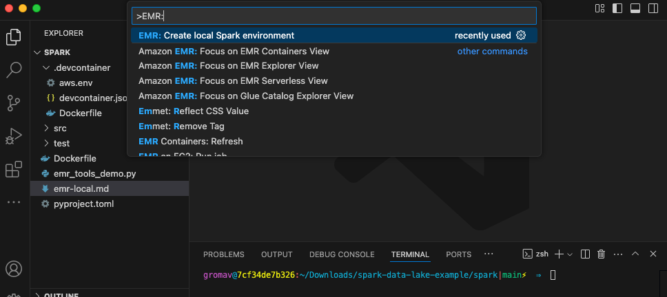
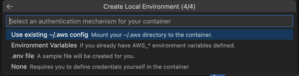
Amazon SageMaker Lakehouse now supports attribute-based access control

Post Syndicated from Sandeep Adwankar original https://aws.amazon.com/blogs/big-data/amazon-sagemaker-lakehouse-now-supports-attribute-based-access-control/

Amazon SageMaker Lakehouse now supports attribute-based access control (ABAC) with AWS Lake Formation, using AWS Identity and Access Management (IAM) principals and session tags to simplify data access, grant creation, and maintenance. With ABAC, you can manage business attributes associated with user identities and enable organizations to create dynamic access control policies that adapt to the specific context.

SageMaker Lakehouse is a unified, open, and secure data lakehouse that now supports ABAC to provide unified access to general purpose Amazon S3 buckets, Amazon S3 Tables, Amazon Redshift data warehouses, and data sources such as Amazon DynamoDB or PostgreSQL. You can then query, analyze, and join the data using Redshift, Amazon AthenaAmazon EMR, and AWS Glue. You can secure and centrally manage your data in the lakehouse by defining fine-grained permissions with Lake Formation that are consistently applied across all analytics and machine learning(ML) tools and engines. In addition to its support for role-based and tag-based access control, Lake Formation extends support to attribute-based access to simplify data access management for SageMaker Lakehouse, with the following benefits:

  • Flexibility – ABAC policies are flexible and can be updated to meet changing business needs. Instead of creating new rigid roles, ABAC systems allow access rules to be modified by simply changing user or resource attributes.
  • Efficiency – Managing a smaller number of roles and policies is more straightforward than managing a large number of roles, reducing administrative overhead.
  • Scalability – ABAC systems are more scalable for larger enterprises because they can handle a large number of users and resources without requiring a large number of roles.

Attribute-based access control overview

Previously, within SageMaker Lakehouse, Lake Formation granted access to resources based on the identity of a requesting user. Our customers were requesting the capability to express the full complexity required for access control rules in organizations. ABAC allows for more flexible and nuanced access policies that can better reflect real-world needs. Organizations can now grant permissions on a resource based on user attribute and is context-driven. This allows administrators to grant permissions on a resource with conditions that specify user attribute keys and values. IAM principals with matching IAM or session tag key-value pairs will gain access to the resource.

Instead of creating a separate role for each team member’s access to a specific project, you can set up ABAC policies to grant access based on attributes like membership and user role, reducing the number of roles required. For instance, without ABAC, a company with an account manager role that covers five different geographical territories needs to create five different IAM roles and grant data access for only the specific territory for which the IAM role is meant. With ABAC, they can simply add those territory attributes as keys/values to the principal tag and provide data access grants based on those attributes. If the value of the attribute for a user changes, access to the dataset will automatically be invalidated.

With ABAC, you can use attributes such as department or country and use IAM or sessions tags to determine access to data, making it more straightforward to create and maintain data access grants. Administrators can define fine-grained access permissions with ABAC to limit access to databases, tables, rows, columns, or table cells.

In this post, we demonstrate how to get started with ABAC in SageMaker Lakehouse and use with various analytics services.

Solution overview

To illustrate the solution, we are going to consider a fictional company called Example Retail Corp. Example Retail’s leadership is interested in analyzing sales data in Amazon S3 to determine in-demand products, understand customer behavior, and identify trends, for better decision-making and increased profitability. The sales department sets up a team for sales analysis with the following data access requirements:

  • All data analysts in the Sales department in the US get access to only sales-specific data in only US regions
  • All BI analysts in the Sales department have full access to data in only US regions
  • All scientists in the Sales department get access to only sales-specific data across all regions
  • Anyone outside of Sales department have no access to sales data

For this post, we consider the database salesdb, which contains the store_sales table that has store sales details. The table store_sales has the following schema.

To demonstrate the product sales analysis use case, we will consider the following personas from the Example Retail Corp:

  • Ava is a data administrator in Example Retail Corp who is responsible for supporting team members with specific data permission policies
  • Alice is a data analyst who should be able to access sales specific US store data to perform product sales analysis
  • Bob is a BI analyst who should be able to access all data from US store sales to generate reports
  • Charlie is a data scientist who should be able to access sales specific across all regions to explore and find patterns for trend analysis

Ava decides to use SageMaker Lakehouse to unify data across various data sources while setting up fine-grained access control using ABAC. Alice is excited about this decision as she can now build daily reports using her expertise with Athena. Bob now knows that he can quickly build Amazon QuickSight dashboards with queries that are optimized using Redshift’s cost-based optimizer. Charlie, being an open source Apache Spark contributor, is excited that he can build Spark based processing with Amazon EMR to build ML forecasting models.

Ava defines the user attributes as static IAM tags that could also include attributes stored in the identity provider (IdP) or as session tags dynamically to represent the user metadata. These tags are assigned to IAM users or roles and can be used to define or restrict access to specific resources or data. For more details, refer to Tags for AWS Identity and Access Management resources and Pass session tags in AWS STS.

For this post, Ava assigns users with static IAM tags to represent the user attributes, including their department membership, Region assignment, and current role relationship. The following table summarizes the tags that represent user attributes and user assignment.

User Persona Attributes Access
Alice Data Analyst Department=sales
Region=US
Role=Analyst
Sales specific data in US and no access to customer data
Bob BI Analyst Department=sales
Region=US
Role=BIAnalyst
All data in US
Charlie Data Scientist Department=sales
Region=ALL
Role=Scientist
Sales specific data in All regions and no access to customer data

Ava then defines access control policies in Lake Formation that grant or restrict access to certain resources based on predefined criteria (user attributes defined using IAM tags) being satisfied. This allows for flexible and context-aware security policies where access privileges can be adjusted dynamically by modifying the user attribute assignment without changing the policy rules. The following table summarizes the policies in the Sales department.

Access User Attributes Policy
All analysts (including Alice) in US get access to sales specific data in US regions Department=sales
Region=US
Role=Analyst
Table: store_sales (store_id, transaction_date, product_name, country, sales_price, quantity columns)
Row filter: country='US'
All BI analysts (including Bob) in US get access to all data in US regions Department=sales
Region=US
Role=BIAnalyst
Table: store_sales (all columns)
Row filter: country='US'
All scientists (including Charlie) get access to sales-specific data from all regions Department=sales
Region=ALL
Role=Scientist
Table: store_sales (all rows)
Column filter: store_id, transaction_date, product_name, country, sales_price,quantity

The following diagram illustrates the solution architecture.

Implementing this solution consists of the following high-level steps. For Example Retail, Ava as a data Administrator performs these steps:

  1. Define the user attributes and assign them to the principal.
  2. Grant permission on the resources (database and table) to the principal based on user attributes.
  3. Verify the permissions by querying the data using various analytics services.

Prerequisites

To follow the steps in this post, you must complete the following prerequisites:

  1. AWS account with access to the following AWS services:
    • Amazon S3
    • AWS Lake Formation and AWS Glue Data Catalog
    • Amazon Redshift
    • Amazon Athena
    • Amazon EMR
    • AWS Identity and Access Management (IAM)
  1. Set up an admin user for Ava. For instructions, see Create a user with administrative access.
  2. Setup S3 bucket for uploading script.
  3. Set up a data lake admin. For instructions, see Create a data lake administrator.
  4. Create IAM user named Alice and attach permissions for Athena access. For instructions, refer to Data analyst permissions.
  5. Create IAM user Bob and attach permissions for Redshift access.
  6. Create IAM user Charlie and attach permissions for EMR Serverless access.
  7. Create job runtime role: scientist_role and that will be used by Charlie. For instruction refer to: Job runtime roles for Amazon EMR Serverless
  8. Setup EMR Serverless application with Lake Formation enabled. For instruction refer to: Using EMR Serverless with AWS Lake Formation for fine-grained access control
  9. Have an existing AWS Glue database or table and Amazon Simple Storage Service (Amazon) S3 bucket that holds the table data. For this post, we use salesdb as our database, store_sales as our table, and data is stored in an S3 bucket.

Define attributes for the IAM principals Alice, Bob, Charlie

Ava completes the following steps to define the attributes for the IAM principal:

  1. Log in as an admin user and navigate to the IAM console.
  2. Choose Users under Access management in the navigation pane and search for the user Alice.
  3. Choose the user and choose the Tags tab.
  4. Choose Add new tag and provide the following key pairs:
    • Key: Department and value: sales
    • Key: Region and value: US
    • Key: Role and value: Analyst
  5. Choose Save changes.
  6. Repeat the process for the user Bob and provide the following key pairs:
    • Key: Department and value: sales
    • Key: Region and value: US
    • Key: Role and value: BIAnalyst
  7. Repeat the process for the user Charlie and IAM role scientist_role and provide the following key pairs:
    • Key: Department and value: sales
    • Key: Region and value: ALL
    • Key: Role and value: Scientist

Grant permissions to Alice, Bob, Charlie using ABAC

Ava now grants database and table permissions to users with ABAC.

Grant database permissions

Complete the following steps:

  1. Ava logs in as data lake admin and navigate to the Lake Formation console.
  2. In the navigation pane, under Permissions, choose Data lake permissions.
  3. Choose Grant.
  4. On the Grant permissions page, choose Principals by attribute.
  5. Specify the following attributes:
    • Key: Department  and value: sales
    • Key: Role and value: Analyst,Scientist
  6. Review the resulting policy expression.
  7. For Permission scope, select This account.
  8. Next, choose the catalog resources to grant access:
    • For Catalogs, enter the account ID.
    • For Databases, enter salesdb.
  9. For Database permissions, select Describe.
  10. Choose Grant.

Ava now verifies the database permission by navigating to the Databases tab under the Data Catalog and searching for salesdb. Select salesdb and choose View under Actions.

Grant table permissions to Alice

Complete the following steps to create a data filter to view sales specific columns in store_sales records whose country=US:

  1. On the Lake Formation console, choose Data filters under Data Catalog in the navigation pane.
  2. Choose Create new filter.
  3. Provide the data filter name as us_sales_salesonlydata.
  4. For Target catalog, enter the account ID.
  5. For Target database, choose salesdb.
  6. For Target table, choose store_sales.
  7. For column-level access, choose Include columns: store_id, item_code, transaction_date, product_name, country, sales_price, and quantity.
  8. For Row-level access, choose Filter rows and enter the row filter country='US'.
  9. Choose Create data filter.
  1. On the Grant permissions page, choose Principals by attribute.
  2. Specify the attributes:
    • Key: Department and value: sales
    • Key: Role as value: Analyst
    • Key: Region and value: US
  3. Review the resulting policy expression.
  4. For Permission scope, select This account.
  5. Choose the catalog resources to grant access:
    • Catalogs: Account ID
    • Databases: salesdb
    • Table: store_sales
    • Data filters: us_sales
  6. For Data filter permissions, select Select.
  7. Choose Grant.

Grant table permissions to Bob

Complete the following steps to create a data filter to view only store_sales records whose country=US:

  1. On the Lake Formation console, choose Data filters under Data Catalog in the navigation pane.
  2. Choose Create new filter.
  3. Provide the data filter name as us_sales.
  4. For Target catalog, enter the account ID.
  5. For Target database, choose salesdb.
  6. For Target table, choose store_sales.
  7. Leave Column-level access as Access to all columns.
  8. For Row-level access, enter the row filter country='US'.
  9. Choose Create data filter.

Complete the following steps to grant table permissions to Bob:

  1. On the Grant permissions page, choose Principals by attribute.
  2. Specify the attributes:
    • Key: Department and value: sales
    • Key: Role as value: BIAnalyst
    • Key: Region and value: US
  3. Review the resulting policy expression.
  4. For Permission scope, select This account.
  5. Choose the catalog resources to grant access:
    • Catalogs: Account ID
    • Databases: salesdb
    • Table: store_sales
  6. For Data filter permissions, select Select.
  7. Choose Grant.

Grant table permissions to Charlie

Complete the following steps to grant table permissions to Charlie:

  1. On the Grant permissions page, choose Principals by attribute.
  2. Specify the attributes:
    1. Key: Department and value: sales
    2. Key: Role as value: Scientist
    3. Key: Region and value: ALL
  3. Review the resulting policy expression.
  4. For Permission scope, select This account
  5. Choose the catalog resources to grant access:
    1. Catalogs: Account ID
    2. Databases: salesdb
    3. Table: store_sales
  6. For Table permissions, select Select.
  7. For Data permissions, specify the following columns: store_id, transaction_date, product_name, country, sales_price, and quantity.
  8. Choose Grant.

Alice now verifies the table permission by navigating to the Tables tab under the Data Catalog and searching for store_sales. Select store_sales and choose View under Actions. The following screenshots show the details for both sets of permissions.

Data Analyst uses Athena for building daily sales reports

Alice, the data analyst logs in to the Athena console and run the following query:

select * from "salesdb"."store_sales" limit 5

Alice has the user attributes as Department=sales, Role=Analyst, Region=US, and this attribute combination allows her access to US sales data to specific sales only column, without access to customer data as shown in the following screenshot.

BI Analyst uses Redshift for building sales dashboards

Bob, the BI Analyst, logs in to the Redshift console and run the following query:

select * from "salesdb"."store_sales" limit 10

Bob has the user attributes Department=sales, Role=BIAnalyst, Region=US, and this attribute combination allows him access to all columns including customer data for US sales data.

Data Scientist uses Amazon EMR to process sales data

Finally, Charlie logs in to the EMR console and submit the EMR job with runtime role as scientist_role. Charlie uses  the script sales_analysis.py that is uploaded to s3 bucket created for the script. He chooses the EMR Serverless application created with Lake Formation enabled.

Charlie submits batch job runs by choosing the following values:

  • Name: sales_analysis_Charlie
  • Runtime_role: scientist_role
  • Script location: <s3_script_path>/sales_analysis.py
  • For spark properties, provide key as spark.emr-serverless.lakeformation.enabled and value as true.
  • Additional configurations: Under Metastore configuration select Use AWS Glue Data Catalog as metastore. Charlie keeps rest of the configuration as default.

Once the job run is completed, Charlie can view the output by selecting stdout under Driver log files.

Charlie uses scientist_role as job runtime role with the attributes Department=sales, Role=Scientist, Region=ALL, and this attribute combination allows him access to select columns of all sales data.

Clean up

Complete the following steps to delete the resources you created to avoid unexpected costs:

  1. Delete the IAM users created.
  2. Delete the AWS Glue database and table resources created for the post, if any.
  3. Delete the Athena, Redshift and EMR resources created for the post.

Conclusion

In this post, we showcased how you can use SageMaker Lakehouse attribute-based access control, using IAM principals and session tags to simplify data access, grant creation, and maintenance. With attribute-based access control, you can manage permissions using dynamic business attributes associated with user identities and secure your data in the lakehouse by defining fine-grained permissions in the Lake Formation that are enforced across analytics and ML tools and engines.

For more information, refer to documentation. We encourage you to try out the SageMaker Lakehouse with ABAC and share your feedback with us.


About the authors

Sandeep Adwankar is a Senior Product Manager at AWS. Based in the California Bay Area, he works with customers around the globe to translate business and technical requirements into products that enable customers to improve how they manage, secure, and access data.

Srividya Parthasarathy is a Senior Big Data Architect on the AWS Lake Formation team. She enjoys building data mesh solutions and sharing them with the community.

Read and write Apache Iceberg tables using AWS Lake Formation hybrid access mode

Post Syndicated from Aarthi Srinivasan original https://aws.amazon.com/blogs/big-data/read-and-write-apache-iceberg-tables-using-aws-lake-formation-hybrid-access-mode/

Enterprises are adopting Apache Iceberg table format for its multitude of benefits. The change data capture (CDC), ACID compliance, and schema evolution features cater to representing big datasets that receive new records at a fast pace. In an earlier blog post, we discussed how to implement fine-grained access control in Amazon EMR Serverless using AWS Lake Formation for reads. Lake Formation helps you centrally manage and scale fine-grained data access permissions and share data with confidence within and outside your organization.

In this post, we demonstrate how to use Lake Formation for read access while continuing to use AWS Identity and Access Management (IAM) policy-based permissions for write workloads that update the schema and upsert (insert and update combined) data records into the Iceberg tables. The bimodal permissions are needed to support existing data pipelines that use only IAM and Amazon Simple Storage Service (Amazon) S3 bucket policy-based permissions and to support table operations that are not yet available in the analytics engines. The two-way permission is achieved by registering the Amazon S3 data location of the Iceberg table with Lake Formation in hybrid access mode. Lake Formation hybrid access mode allows you to onboard new users with Lake Formation permissions to access AWS Glue Data Catalog tables with minimal interruptions to existing IAM policy-based users. With this solution, organizations can use the Lake Formation permissions to scale the access of their existing Iceberg tables in Amazon S3 to new readers. You can extend the methodology to other open table formats, such as Linux Foundation Delta Lake tables and Apache Hudi tables.

Key use cases for Lake Formation hybrid access mode

Lake Formation hybrid access mode is useful in the following use cases:

  • Avoiding data replication – Hybrid access mode helps onboard new users with Lake Formation permissions on existing Data Catalog tables. For example, you can enable a subset of data access (coarse vs. fine-grained access) for various user personas, such as data scientists and data analysts, without making multiple copies of the data. This also helps maintain a single source of truth for production and business insights.
  • Minimal interruption to existing IAM policy-based user access – With hybrid access mode, you can add new Lake Formation managed users with minimal disruptions to your existing IAM and Data Catalog policy-based user access. Both access methods can coexist for the same catalog table, but each user can have only one mode of permissions.
  • Transactional table writes – Certain write operations like insert, update, and delete are not supported by Amazon EMR for Lake Formation managed Iceberg tables. Refer to Considerations and limitations for additional details. Although you could use Lake Formation permissions for Iceberg table read operations, you could manage the write operations as the table owners with IAM policy-based access.

Solution overview

An example Enterprise Corp has a large number of Iceberg tables based on Amazon S3. They are currently managing the Iceberg tables manually with IAM policy, Data Catalog resource policy, and S3 bucket policy-based access in their organization. They want to share their transactional data of Iceberg tables across different teams, such as data analysts and data scientists, asking for read access across a few lines of business. While maintaining the ownership of the table’s updates to their single team, they want to provide restricted read access to certain columns of their tables. This is achieved by using the hybrid access mode feature of Lake Formation.

In this post, we illustrate the scenario with a data engineer team and a new data analyst team. The data engineering team owns the extract, transform, and load (ETL) application that will process the raw data to create and maintain the Iceberg tables. The data analyst team will query the tables to gather business insights from those tables. The ETL application will use IAM role-based access to the Iceberg table, and the data analyst gets Lake Formation permissions to query the same tables.

The solution can be visually represented in the following diagram.

Solution Overview

For ease of illustration, we use only one AWS account in this post. Enterprise use cases typically have multiple accounts or cross-account access requirements. The setup of the Iceberg tables, Lake Formation permissions, and IAM based permissions are similar for multiple and cross-account scenarios.

The high-level steps involved in the permissions setup are as follows:

  1. Make sure that IAMAllowedPrincipals has Super access to the database and tables in Lake Formation. IAMAllowedPrincipals is a virtual group that represents any IAM principal permissions. Super access to this virtual group is required to make sure that IAM policy-based permissions to any IAM principal continues to work.
  2. Register the data location with Lake Formation in hybrid access mode.
  3. Grant DATA LOCATION permission to the IAM role that manages the table with IAM policy-based permissions. Without the DATA LOCATION permission, write workloads will fail. Test the access to the table by writing new records to the table as the IAM role.
  4. Add SELECT table permissions to the Data-Analyst role in Lake Formation.
  5. Opt-in the Data-Analyst to the Iceberg table, making the Lake Formation permissions effective for the analyst.
  6. Test access to the table as the Data-Analyst by running SELECT queries in Athena.
  7. Test the table write operations by adding new records to the table as ETL-application-role using EMR Serverless.
  8. Read the latest update, again, as Data-Analyst.

Prerequisites

You should have the following prerequisites:

  • An AWS account with a Lake Formation administrator configured. Refer to Data lake administrator permissions and Set up AWS Lake Formation. You can also refer to Simplify data access for your enterprise using Amazon SageMaker Lakehouse for the Lake Formation admin setup in your AWS account. For ease of demonstration, we have used an IAM admin role added as a Lake Formation administrator.
  • An S3 bucket to host the sample Iceberg table data and metadata.
  • An IAM role to register your Iceberg table Amazon S3 location with Lake Formation. Follow the policy and trust policy details for a user-defined role creation from Requirements for roles used to register locations.
  • An IAM role named ETL-application-role, which will be the runtime role to execute jobs in EMR Serverless. The minimum policy required is shown in the following code snippet. Replace the Amazon S3 data location of the Iceberg table, database name, and AWS Key Management Service (AWS KMS) key ID with your own. For additional details on the role setup, refer to Job runtime roles for Amazon EMR Serverless. This role can insert, update, and delete data in the table.
    {
        "Version": "2012-10-17",
        "Statement": [
            {
                "Sid": "IcebergDataAccessInS3",
                "Effect": "Allow",
                "Action": [
                    "s3:ListBucket",
                    "s3:GetBucketLocation",
                    "s3:ListAllMyBuckets",
                    "s3:Get*",
                    "s3:Put*",
                    "s3:Delete*"
                ],
                "Resource": [
                    "arn:aws:s3:::your-iceberg-data-bucket-name",
                    "arn:aws:s3:::your-iceberg-data-bucket-name/*"
                ]
            },
            {
                "Sid": "GlueCatalogApiPermissions",
                "Effect": "Allow",
                "Action": [
                    "glue:*"
                ],
                "Resource": [
                    "arn:aws:glue:your-Region:account-id:catalog",
                    "arn:aws:glue:your-Region:account-id:database/iceberg-database-name",
                    "arn:aws:glue:your-Region:account-id:database/default",
                    "arn:aws:glue:your-Region:account-id:table/*/*"
                ]
            },
            {
                "Sid": "KmsKeyPermissions",
                "Effect": "Allow",
                "Action": [
                    "kms:Encrypt",
                    "kms:Decrypt",
                    "kms:ReEncrypt*",
                    "kms:GenerateDataKey",
                    "kms:DescribeKey",
                    "kms:ListKeys",
                    "kms:ListAliases"
                ],
                "Resource": [
                    "arn:aws:kms:your-Region:account-id:key/your-key-id"
                ]
            }
        ]
    }

    Add the following trust policy to the role:

    {
        "Version": "2012-10-17",
        "Statement": [
            {
                "Effect": "Allow",
                "Principal": {
                    "Service": "emr-serverless.amazonaws.com"
                },
                "Action": "sts:AssumeRole"
            }
        ]
    }

  • An IAM role called Data-Analyst, to represent the data analyst access. Use the following policy to create the role. Also attach the AWS managed policy arn:aws:iam::aws:policy/AmazonAthenaFullAccess to the role, to allow querying the Iceberg table using Amazon Athena. Refer to Data engineer permissions for additional details about this role.
    {
        "Version": "2012-10-17",
        "Statement": [
            {
                "Sid": "LFBasicUser",
                "Effect": "Allow",
                "Action": [
                    "glue:GetCatalog",
                    "glue:GetCatalogs",
                    "glue:GetTable",
                    "glue:GetTables",
                    "glue:GetTableVersion",
                    "glue:GetTableVersions",
                    "glue:GetDatabase",
                    "glue:GetDatabases",
                    "glue:GetPartition",
                    "glue:GetPartitions",
                    "lakeformation:GetDataAccess"
                ],
                "Resource": "*"
            },
            {
                "Sid": "AthenaResultsBucket",
                "Effect": "Allow",
                "Action": [
                    "s3:ListBucket",
                    "s3:GetBucketLocation",
                    "s3:Put*",
                    "s3:Get*",
                    "s3:Delete*"
                ],
                "Resource": [
                    "arn:aws:s3:::your-bucket-name-prefix",
                    "arn:aws:s3:::your-bucket-name-prefix/*"
                ]
            }
        ]
    }

    Add the following trust policy to the role:

    {
        "Version": "2012-10-17",
        "Statement": [
            {
                "Effect": "Allow",
                "Principal": {
                    "AWS": "arn:aws:iam::<your_account_id>:root"
                },
                "Action": "sts:AssumeRole"
            }
        ]
    }

Create the Iceberg table

Complete the following steps to create the Iceberg table:

  1. Sign in to the Lake Formation console as the admin role.
  2. In the navigation pane under Data Catalog, choose Databases.
  3. From the Create dropdown menu, create a database named iceberg_db. You can leave the Amazon S3 location property empty for the database.
  4. On the Athena console, run the following provided queries. The queries perform the following operations:
    1. Create a table called customer_csv, pointing to the customer dataset in the public S3 bucket.
    2. Create an Iceberg table called customer_iceberg, pointing to your S3 bucket location that will host the Iceberg table data and metadata.
    3. Insert data from the CSV table to the Iceberg table.
      CREATE EXTERNAL TABLE `iceberg_db`.`customer_csv`(
        `c_customer_sk` int,
        `c_customer_id` string,
        `c_current_cdemo_sk` int,
        `c_current_hdemo_sk` int,
        `c_current_addr_sk` int,
        `c_first_shipto_date_sk` int,
        `c_first_sales_date_sk` int,
        `c_salutation` string,
        `c_first_name` string,
        `c_last_name` string,
        `c_preferred_cust_flag` string,
        `c_birth_day` int,
        `c_birth_month` int,
        `c_birth_year` int,
        `c_birth_country` string,
        `c_login` string,
        `c_email_address` string,
        `c_last_review_date` string)
      ROW FORMAT DELIMITED
        FIELDS TERMINATED BY '|'
      STORED AS INPUTFORMAT
        'org.apache.hadoop.mapred.TextInputFormat'
      OUTPUTFORMAT
        'org.apache.hadoop.hive.ql.io.HiveIgnoreKeyTextOutputFormat'
      LOCATION
        ' s3://redshift-downloads/TPC-DS/2.13/10GB/customer/'
      TBLPROPERTIES (
        'classification'='csv');   
      
       SELECT * FROM customer_csv LIMIT 5; //verifies table data  
      
      CREATE TABLE IF NOT EXISTS iceberg_db.customer_iceberg (
              c_customer_sk             int,
              c_customer_id             string,
              c_current_cdemo_sk        int,
              c_current_hdemo_sk        int,
              c_current_addr_sk         int,
              c_first_shipto_date_sk    int,
              c_first_sales_date_sk     int,
              c_salutation              string,
              c_first_name              string,
              c_last_name               string,
              c_preferred_cust_flag     string,
              c_birth_day               int,
              c_birth_month             int,
              c_birth_year              int,
              c_birth_country           string,
              c_login                   string,
              c_email_address           string,
              c_last_review_date        string
          )
      LOCATION 's3://your-iceberg-data-bucket-name/path/'
      TBLPROPERTIES ( 'table_type' = 'ICEBERG' );
      
      INSERT INTO customer_iceberg
      SELECT *
      FROM customer_csv;  
      
      SELECT * FROM customer_iceberg LIMIT 5; //verifies table data

Set up the Iceberg table as a hybrid access mode resource

Complete the following steps to set up the Iceberg table’s Amazon S3 data location as hybrid access mode in Lake Formation:

  1. Register your table location with Lake Formation:
    1. Sign in to the Lake Formation console as data lake administrator.
    2. In the navigation pane, choose Data lake Locations.
    3. For Amazon S3 path, provide the S3 prefix of your Iceberg table location that holds both the data and metadata of the table.
    4. For IAM role, provide the user-defined role that has permissions to your Iceberg table’s Amazon S3 location and that you created according to the prerequisites. For more details, refer to Registering an Amazon S3 location.
    5. For Permission mode, select Hybrid access mode.
    6. Choose Register location to register your Iceberg table Amazon S3 location with Lake Formation.

  1. Add data location permission to ETL-application-role:
    1. In the navigation pane, choose Data locations.
    2. For IAM users and roles, choose ETL-application-role.
    3. For Storage location, provide the S3 prefix of your Iceberg table.
    4. Choose Grant.

Data location permission is required for write operations to the Iceberg table location only if the Iceberg table’s S3 prefix is a child location of the database’s Amazon S3 location property.

  1. Grant Super access on the Iceberg database and table to IAMAllowedPrincipals:
    1. In the navigation pane, choose Data permissions.
    2. Choose IAM users and roles and choose IAMAllowedPrincipals.
    3. For LF-Tags or catalog resources, choose Named Data Catalog resources.
    4. Under Databases, select the name of your Iceberg table’s database.
    5. Under Database permissions, select Super.
    6. Choose Grant.

    7. Repeat the preceding steps and for Tables – optional, choose the Iceberg table.
    8. Under Table permissions, select Super.
    9. Choose Grant.

  1. Add database and table permissions to the Data-Analyst role:
    1. Repeat the steps in Step 3 to grant permissions for the Data-Analyst role, once for database-level permission and once for table-level permission.
    2. Select Describe permissions for the Iceberg database.
    3. Select Select permissions for the Iceberg table.
    4. Under Hybrid access mode, select Make Lake Formation permissions effective immediately.
    5. Choose Grant.

The following screenshots show the database permissions for Data-Analyst.

The following screenshots show the table permissions for Data-Analyst.

  1. Verify Lake Formation permissions on the Iceberg table and database to both Data-Analyst and IAMAllowedPrincipals:
    1. In the navigation pane, choose Data permissions.
    2. Filter by Table= customer_iceberg.
      You should see IAMAllowedPrincipals with All permission and Data-Analyst with Select permission.
    3. Similarly, verify permissions for the database by filtering database=iceberg_db.

You should see IAMAllowedPrincipals with All permission and Data-Analyst with Describe permission.

  1. Verify Lake Formation opt-in for Data-Analyst:
    1. In the navigation pane, choose Hybrid access mode.

You should see Data-Analyst opted-in for both database and table level permissions.

Query the table as the Data-Analyst role in Athena

While you are logged in to the AWS Management Console as admin, set up the Athena query results bucket:

  1. On the console navigation bar, choose your user name.
  2. Choose Switch role to switch to the Data-Analyst role.
  3. Enter your account ID, IAM role name (Data-Analyst), and choose Switch Role.
  4. Now that you’re logged in as the Data-Analyst role, open the Athena console and set up the Athena query results bucket.
  5. Run the following query to read the Iceberg table. This verifies the Select permission granted to the Data-Analyst role in Lake Formation.
SELECT * FROM "iceberg_db"."customer_iceberg"
WHERE c_customer_sk = 247

Upsert data as ETL-application-role using Amazon EMR

To upsert data to Lake Formation enabled Iceberg tables, we will use Amazon EMR Studio, which is an integrated development environment (IDE) that makes it straightforward for data scientists and data engineers to develop, visualize, and debug data engineering and data science applications written in R, Python, Scala, and PySpark. EMR Studio will be our web-based IDE to run our notebooks, and we will use EMR Serverless as the compute engine. EMR Serverless is a deployment option for Amazon EMR that provides a serverless runtime environment. For the steps to run an interactive notebook, see Submit a job run or interactive workload.

  1. Sign out of the AWS console as Data-Analyst and log back or switch the user to admin.
  2. On the Amazon EMR console, choose EMR Serverless in the navigation pane.
  3. Choose Get started.
  4. For first-time users, Amazon EMR allows creation of an EMR Studio without a virtual private cloud (VPC). Create an EMR Serverless application as follows:
    1. Provide a name for the EMR Serverless application, such as DemoHybridAccess.
    2. Under Application setup, choose Use default settings for interactive workloads.
    3. Choose Create and start application.

The next step is to create an EMR Studio.

  1. On the Amazon EMR console, choose Studio under EMR Studio in the navigation pane.
  2. Choose Create Studio.
  3. Select Interactive workloads.
  4. You should see a default pre-populated section. Keep these default settings and choose Create Studio and launch Workspace.

  1. After the workspace is launched, attach the EMR Serverless application created earlier and select ETL-application-role as the runtime role under Compute.

  1. Download the notebook Iceberg-hybridaccess_final.ipynb and upload it to EMR Studio workspace.

This notebook configures the metastore properties to work with Iceberg tables. (For more details, see Using Apache Iceberg with EMR Serverless.) Then it performs insert, update, and delete operations in the Iceberg table. It also verifies if the operations are successful by reading the newly added data.

  1. Select PySpark as the kernel and execute each cell in the notebook by choosing the run icon.

Refer to Submit a job run or interactive workload for further details about how to run an interactive notebook.

The following screenshot shows that the Iceberg table insert operation completed successfully.

The following screenshot illustrates running the update statement on the Iceberg table in the notebook.

The following screenshot shows that the Iceberg table delete operation completed successfully.

Query the table again as Data-Analyst using Athena

Complete the following steps:

  1. Switch your role to Data-Analyst on the AWS console.
  2. Run the following query on the Iceberg table and read the row that was updated by the EMR cluster:
    SELECT * FROM "iceberg_db"."customer_iceberg"
    WHERE c_customer_sk = 247

The following screenshot shows the results. As we can see, ‘c_first_name’ column is updated with new value.

Clean up

To avoid incurring costs, clean up the resources you used for this post:

  1. Revoke the Lake Formation permissions and hybrid access mode opt-in granted to the Data-Analyst role and IAMAllowedPrincipals.
  2. Revoke the registration of the S3 bucket to Lake Formation.
  3. Delete the Athena query results from your S3 bucket.
  4. Delete the EMR Serverless resources.
  5. Delete Data-Analyst role and ETL-application-role from IAM.

Conclusion

In this post, we demonstrated how to scale the adoption and use of Iceberg tables using Lake Formation permissions for read workloads, while maintaining full control over table schema and data updates through IAM policy-based permissions for the table owners. The methodology also applies to other open table formats and standard Data Catalog tables, but the Apache Spark configuration for each open table format will vary.

Hybrid access mode in Lake Formation is an option you could use to adopt Lake Formation permissions gradually and scale those use cases that support Lake Formation permissions while using IAM based permissions for the use cases that don’t. We encourage you to try out this setup in your environment. Please share your feedback and any additional topics you would like to see in the comments section.


About the Authors

Aarthi Srinivasan is a Senior Big Data Architect with AWS Lake Formation. She collaborates with the service team to enhance product features, works with AWS customers and partners to architect lake house solutions, and establishes best practices.

Parul Saxena is a Senior Big Data Specialist Solutions Architect in AWS. She helps customers and partners build highly optimized, scalable, and secure solutions. She specializes in Amazon EMR, Amazon Athena, and AWS Lake Formation, providing architectural guidance for complex big data workloads and assisting organizations in modernizing their architectures and migrating analytics workloads to AWS.

Build a data lakehouse in a hybrid Environment using Amazon EMR Serverless, Apache DolphinScheduler, and TiDB

Post Syndicated from Shiyang Wei original https://aws.amazon.com/blogs/big-data/build-a-data-lakehouse-in-a-hybrid-environment-using-amazon-emr-serverless-apache-dolphinscheduler-and-tidb/

While helping our customers build systems on AWS, we found out that a large number of enterprise customers who pay great attention to data security and compliance, such as B2C FinTech enterprises, build data-sensitive applications on premises and use other applications on AWS to take advantage AWS managed services. Using AWS managed services can greatly simplify daily operation and maintenance, as well as help you achieve optimized resource utilization and performance.

This post discusses a decoupled approach of building a serverless data lakehouse using AWS Cloud-centered services, including Amazon EMR Serverless, Amazon Athena, Amazon Simple Storage Service (Amazon S3), Apache DolphinScheduler (an open source data job scheduler) as well as PingCAP TiDB, a third-party data warehouse product that can be deployed either on premises or on the cloud or through a software as a service (SaaS).

Solution overview

For our use case, an enterprise data warehouse with business data is hosted on an on-premises TiDB platform, an AWS Global Partner that is also available on AWS through AWS Marketplace.

The data is then processed by an Amazon EMR Serverless Job to achieve data lakehouse tiering logic. Different tiering data are stored in separate S3 buckets or separate S3 prefixes under the same S3 bucket. Typically, there are four layers in terms of data warehouse design.

  1. Operational data store layer (ODS) – This layer stores raw data of the data warehouse
  2. Data warehouse stage layer (DWS) – This layer is a temporary staging area within the data warehousing architecture where data from various sources is loaded, cleaned, transformed, and prepared before being loaded into the data warehouse database layer;
  3. Data warehouse database layer (DWD) – This layer is the central repository in a data warehousing environment where data from various sources is integrated, transformed, and stored in a structured format for analytical purposes;
  4. Analytical data store (ADS) – This layer is a subset of the data warehousing that is specifically designed and optimized for a particular business function, department, or analytical purpose.

For this post, we only use ODS and ADS layers to demonstrate the technical feasibility.

The schema of this data is managed through the AWS Glue Data Catalog, and can be queried using Athena. The EMR Serverless Jobs are orchestrated using Apache DolphinScheduler deployed in cluster mode on Amazon Elasctic Compute Cloud (Amazon EC2) instances, with meta data stored in an Amazon Relational Database Service (Amazon RDS) for MySQL instance.

Using DolphinScheduler as the data lakehouse job orchestrator offers the following advantages:

  • Its distributed architecture allows for better scalability, and the visual DAG designer makes workflow creation more intuitive for team members with varying technical expertise
  • It provides more granular task-level controls and supports a wider range of task types out-of-the-box, including Spark, Flink, and machine learning (ML) workflows, without requiring additional plugin installations;
  • Its multi-tenancy feature enables better resource isolation and access control across different teams within an organization.

However, DolphinScheduler requires more initial setup and maintenance effort, making it more suitable for organizations with strong DevOps capabilities and a desire for complete control over their workflow infrastructure.

The following diagram illustrates the solution architecture.

Prerequisites

You need to create an AWS account and set up an AWS Identity and Access Management (IAM) user as a prerequisite for the following implementation. Complete the following steps:

For AWS account signing up, please follow up the actions guided per page link.

  1. Create an AWS account.
  2. Sign in to the account using the root user for the first time.
  3. One the IAM console, create an IAM user with AdministratorAccess Policy.
  4. Use this IAM user to log in AWS Management Console rather the root user.
  5. On the IAM console, choose Users in the navigation pane.
  6. Navigate to your user, and on the Security credentials tab, create an access key.
  7. Store the access key and secret key in a secure place and use them for further API access of the resources of this AWS account.

Set up DolphinScheduler, IAM configuration, and the TiDB Cloud table

In this section, we walk through the steps to install DolphinScheduler, complete additional IAM configurations to enable the EMR Serverless job, and provision the TiDB Cloud table.

Install DolphinScheduler on an EC2 instance with an RDS for MySQL instance storing DolphinScheduler metadata. The production deployment mode of DolphinScheduler is cluster mode. In this blog, we use pseudo cluster mode which has the same installation steps as cluster mode, and could achieve resource economy. We name the EC2 instance ds-pseudo.

Make sure the inbound rule of the security group attached to the EC2 instance allows port 12345’s TCP traffic. Then complete the following steps:

  1. Log in to Amazon EC2 as the root user, and install jvm:
    sudo dnf install java-1.8.0-amazon-corretto
    java -version

  2. Switch to dir /usr/local/src:
    cd /usr/local/src
  3. Install Apache Zookeeper:
    wget https://archive.apache.org/dist/zookeeper/zookeeper-3.8.0/apache-zookeeper-3.8.0-bin.tar.gz
    tar -zxvf apache-zookeeper-3.8.0-bin.tar.gz
    cd apache-zookeeper-3.8.0-bin/conf
    cp zoo_sample.cfg zoo.cfg
    cd ..
    nohup bin/zkServer.sh start-foreground &> nohup_zk.out &
    bin/zkServer.sh status

  4. Check the Python version:
    python3 --version

    The version should be 3.9 or above. It is recommended that you use Amazon Linux 2023 or later as the Amazon EC2 operating system (OS); Python version 3.9 meets the requirement. For detail information, refer to Python in AL2023.

  5. Install Dolphinscheduler
    1. Download the dolphinscheduler package:
      cd /usr/local/src
      wget https://dlcdn.apache.org/dolphinscheduler/3.1.9/apache-dolphinscheduler-3.1.9-bin.tar.gz
      tar -zxvf apache-dolphinscheduler-3.1.9-bin.tar.gz
      mv apache-dolphinscheduler-3.1.9-bin apache-dolphinscheduler
    2. Download the mysql connector package:
      wget https://downloads.mysql.com/archives/get/p/3/file/mysql-connector-j-8.0.31.tar.gz
      tar -zxvf mysql-connector-j-8.0.31.tar.gz
    3. Copy specific mysql connector JAR file to the following destinations:
      cp mysql-connector-j-8.0.31/mysql-connector-j-8.0.31.jar ./apache-dolphinscheduler/api-server/libs/
      cp mysql-connector-j-8.0.31/mysql-connector-j-8.0.31.jar ./apache-dolphinscheduler/alert-server/libs/
      cp mysql-connector-j-8.0.31/mysql-connector-j-8.0.31.jar ./apache-dolphinscheduler/master-server/libs/
      cp mysql-connector-j-8.0.31/mysql-connector-j-8.0.31.jar ./apache-dolphinscheduler/worker-server/libs/
      cp mysql-connector-j-8.0.31/mysql-connector-j-8.0.31.jar ./apache-dolphinscheduler/tools/libs/
    4. Add the user dolphinscheduler, and make sure the directory apache-dolphinscheduler and the files under it are owned by the user dolphinscheduler:
      useradd dolphinscheduler
      echo "dolphinscheduler" | passwd --stdin dolphinscheduler
      sed -i '$adolphinscheduler ALL=(ALL) NOPASSWD: NOPASSWD: ALL' /etc/sudoers
      sed -i 's/Defaults   requirett/#Defaults requirett/g' /etc/sudoers
      chown -R dolphinscheduler:dolphinscheduler apache-dolphinscheduler
  6. Install the mysql client:
    sudo dnf update -y 
    sudo dnf install mariadb105
  7. On the Amazon RDS console, provision an RDS for MySQL instance with the following configurations:
    1. For Database Creation Method, select Standard create.
    2. For Engine options, choose MySQL.
    3. For Edition: choose MySQL 8.0.35.
    4. For Templates: select Dev/Test.
    5. For Availability and durability, select Single DB instance.
    6. For Credentials management, select Self-managed.
    7. For Connectivity, select Connect to an EC2 compute resource, and choose the EC2 instance created earlier.
    8. For Database Authentication: choose Password Authentication.
  8. Navigate to the ds- mysql database details page, and under Connectivity & security, copy the RDS for MySQL endpoint.
  9. Configure the intance:
    mysql -h <RDS for mysql Endpoint> -u admin -p
    mysql> CREATE DATABASE dolphinscheduler DEFAULT CHARACTER SET utf8 DEFAULT COLLATE utf8_general_ci;
    mysql> exit;
  10. Configure the dolphinscheduler configuration file:
    cd /usr/local/src/apache-dolphinscheduler/
  11. Revise dolphinscheduler_env.sh:
    vim bin/env/dolphinscheduler_env.sh
    export DATABASE=${DATABASE:-mysql}
    export SPRING_PROFILES_ACTIVE=${DATABASE}
    export SPRING_DATASOURCE_URL="jdbc:mysql://ds-mysql.cq**********.us-east-1.rds.amazonaws.com/dolphinscheduler?useUnicode=true&amp;characterEncoding=UTF-8&amp;useSSL=false"
    export SPRING_DATASOURCE_USERNAME="admin"
    export SPRING_DATASOURCE_PASSWORD="<your password>"
  12. On the Amazon EC2 console, navigate to the instance details page and copy the private IP address.
  13. Revise install_env.sh:
    vim bin/env/install_env.sh
    ips=${ips:-"<private ip address of ds-pseudo EC2 instance>"}
    masters=${masters:-"<private ip address of ds-pseudo EC2 instance>"}
    workers=${workers:-" private ip address of ds-pseudo EC2 instance:default"}
    alertServer=${alertServer:-" private ip address of ds-pseudo EC2 instance "}
    apiServers=${apiServers:-" private ip address of ds-pseudo EC2 instance "}
    installPath=${installPath:-"~/dolphinscheduler"}
    export JAVA_HOME=${JAVA_HOME:-/usr/lib/jvm/jre-1.8.0-openjdk}
    export PYTHON_HOME=${PYTHON_HOME:-/bin/python3}
  14. Configure the dolphinscheduler configuration file:
    cd /usr/local/src/apache-dolphinscheduler/
    bash tools/bin/upgrade-schema.sh
  15. Install DolphinScheduler:
    cd /usr/local/src/apache-dolphinscheduler/
    su dolphinscheduler
    bash ./bin/install.sh
  16. Start DolphinScheduler after installation:
    cd /usr/local/src/apache-dolphinscheduler/
    su dolphinscheduler
    bash ./bin/start-all.sh
  17. Open the DolphinScheduler console:
    http://<ec2 ip address>:12345/dolphinscheduler/ui/login

After input the initial username and password, press Login button to enter into the dashboard shown as below.

initial user/password admin/dolphinscheduler123

Configure IAM role to enable the EMR serverless job

The EMR serverless job role needs to have permission to access a specific S3 bucket to read job scripts and potentially write results, and also have permission to access AWS Glue to read the Data Catalog which stores the tables’ meta data. For detailed guidance, please refer to Grant permission to use EMR Serverless or EMR Serverless Samples.

The following screenshot shows the IAM role configured with the trust policy attached.


The IAM role should have the following permissions policies attached, as shown in the following screenshot.

Provision the TiDB Cloud table

  1. To provision the TiDB Cloud table, complete the following steps:
    1. Register for TiDB Cloud.
    2. Create a serverless cluster, as shown in the following screenshot. For this post, we name the cluster Cluster0.
  2. Choose Cluster0, then choose SQL Editor to create a database named test:
    create table testtable (id varchar(255));
    insert into testtable values (1);
    insert into testtable values (2);
    insert into testtable values (3);

Synchronize data between on-premises TiDB and AWS

In this section, we discuss how to synchronize historical data as well as incremental data between TiDB and AWS.

Use TiDB Dumpling to sync historical data from TiDB to Amazon S3

Use the commands in this section to dump data stored in TiDB as CSV files into a S3 bucket. For full details on how to achieve a data sync from on-premises TiDB to Amazon S3, see Export data to Amazon S3 cloud storage. For this post, we use TiDB tool Dumpling. Complete the following steps:

  1. Log in to the EC2 instance created earlier as root.
  2. Run the following command to install TiUP:
    curl --proto '=https' --tlsv1.2 -sSf https://tiup-mirrors.pingcap.com/install.sh | sh
    
    cd /root
    source .bash_profile
    
    tiup --version

  3. Run the following command to install Dumpling:
    tiup install dumpling
  4. Run the following command to achieve target database table dumpling to the specific S3 bucket.
    tiup dumpling -u <prefix.root> -P 4000 -h <tidb serverless endpoint/host> -r 200000 -o "s3://<specific s3 bucket>" --sql "select * from <target database>.<target table>" --ca "/etc/pki/tls/certs/ca-bundle.crt" --password <tidb serverless password>
  5. To acquire the TiDB serverless connection information, navigate to the TiDB Cloud console and choose Connect.

You can collect the specific connection information of test database from the following screenshot.

Yan can view the data stored in the S3 bucket on the Amazon S3 console.

You can use Amazon S3 Select to query the data and get results similar to the following screenshot, confirming that the data has been ingested into testtable.

Use TiDB Dumpling with a self-managed checkpoint to sync incremental data from TiDB to Amazon S3

To achieve incremental data synchronization using TiDB Dumpling, it’s essential to self-manage the check point of the target synchronized data. One recommended way is to store the ID of the final ingested record into a certain media (such as Amazon ElastiCache for Redis, Amazon DynamoDB) to achieve a self-managing checkpoint when running the shell/Python job that trigges TiDB Dumpling. The prerequisite for implementing this is that the target table has a monotonically increasing id field as its primary key.

You can use the following TiDB Dumpling command to filter the exported data:

tiup dumpling -u <prefix.root> -P 4000 -h <tidb serverless endpoint/host> -r 200000 -o "s3://<specific s3 bucket>" --sql "select * from <target database>.<target table> where id > 2" --ca "/etc/pki/tls/certs/ca-bundle.crt" --password <tidb serverless password>

Use the TiDB CDC connector to sync incremental data from TiDB to Amazon S3

The advantage of using TiDB CDC connector to achieve incremental data synchronization from TiDB to Amazon S3 is that there is built-in change data capture (CDC) mechanism, and because the backend engine is Flink, the performance is fast. However, there is one trade-off: you need to create several Flink tables to map the ODS tables on AWS.

For instructions to implement the TiDB CDC connector, refer to TiDB CDC.

Use an EMR serverless job to sync historical and incremental data from a Data Catalog table to the TiDB table

Data usually flows from on premises to the AWS Cloud. However, in some cases, the data might flow from the AWS Cloud to your on-premises database.

After landing on AWS, the data will be wrapped up and managed by the Data Catalog by created Athena tables with the specific tables’ schema. The table DDL script is as follows:

CREATE EXTERNAL TABLE IF NOT EXISTS `testtable`(
  `id` string
) 
ROW FORMAT SERDE 'org.apache.hadoop.hive.serde2.OpenCSVSerde'
LOCATION 's3://<bucket_name>/<prefix_name>/';  

The screenshot below showcases the DDL running result using Athena console.

The data stored in testtable table is queried using select * from testable SQL. The query result is shown as follows:

In this case, an EMR serverless spark job can accomplish the work of synchronizing data from an AWS Glue table to your on premises table.

If the Spark job is written in Scala, the sample code is as below:

package com.example
import org.apache.spark.sql.{DataFrame, SparkSession}

object Main  {

  def main(args: Array[String]): Unit = {

    val spark = SparkSession.builder()
      .appName("<specific app name>")
      .enableHiveSupport()
      .getOrCreate()

    spark.sql("show databases").show()
    spark.sql("use default")
    var df=spark.sql("select * from testtable")

    df.write
      .format("jdbc")
      .option("driver","com.mysql.cj.jdbc.Driver")
      .option("url", "jdbc:mysql://<tidbcloud_endpoint>:4000/namespace")
      .option("dbtable", "<table_name>")
      .option("user", "<user_name>")
      .option("password", "<password_string>")
      .save()

    spark.close()
  }
}

You can acquire the TiDB serverless endpoint connection information on the TiDB console by choosing Connect, as shown earlier in this post.

After you have wrapped the Scala code as JAR file using SBT, you can submit the job to EMR Serverless with the following AWS Command Line Interface (AWS CLI) command:

export applicationId=00fev6mdk***

export job_role_arn=arn:aws:iam::<aws account id>:role/emr-serverless-job-role

aws emr-serverless start-job-run \
    --application-id $applicationId \
    --execution-role-arn $job_role_arn \
    --job-driver '{
        "sparkSubmit": {
            "entryPoint": "<s3 object url for the wrapped jar file>",
            "sparkSubmitParameters": "--conf spark.hadoop.hive.metastore.client.factory.class=com.amazonaws.glue.catalog.metastore.AWSGlueDataCatalogHiveClientFactory --conf spark.driver.cores=1 --conf spark.driver.memory=3g --conf spark.executor.cores=4 --conf spark.executor.memory=3g --jars s3://spark-sql-test-nov23rd/mysql-connector-j-8.2.0.jar"
        }
    }'

If the Spark job is written in PySpark, the sample code is as follows:

import os
import sys
import pyspark.sql.functions as F
from pyspark.sql import SparkSession

if __name__ == "__main__":

    spark = SparkSession\
        .builder\
        .appName("app1")\
        .enableHiveSupport()\
        .getOrCreate()

    df=spark.sql(f"select * from {str(sys.argv[1])}")

    df.write.format("jdbc").options(
        driver="com.mysql.cj.jdbc.Driver",
        url="jdbc:mysql://tidbcloud_endpoint:4000/namespace ",
        dbtable="table_name",
        user="use_name",
        password="password_string").save()

    spark.stop()

You can submit the job to EMR Serverless using the following AWS CLI command:

export applicationId=00fev6mdk***

export job_role_arn=arn:aws:iam::<aws account id>:role/emr-serverless-job-role

aws emr-serverless start-job-run \
    --application-id $applicationId \
    --execution-role-arn $job_role_arn \
    --job-driver '{
        "sparkSubmit": {
            "entryPoint": "<s3 object url for the python script file>",
            "entryPointArguments": ["testspark"],
            "sparkSubmitParameters": "--conf spark.hadoop.hive.metastore.client.factory.class=com.amazonaws.glue.catalog.metastore.AWSGlueDataCatalogHiveClientFactory --conf spark.driver.cores=1 --conf spark.driver.memory=3g --conf spark.executor.cores=4 --conf spark.executor.memory=3g --jars s3://spark-sql-test-nov23rd/mysql-connector-j-8.2.0.jar"
        }
    }'

The preceding PySpark code and AWS CLI command achieves outbound parameter input as well: the table name (specifically testspark) is ingested into the SQL sentence when submitting the job.

EMR Serverless job pperation essentials

An EMR Serverless application is a resource pool concept. An application holds a certain capacity of compute, memory, and storage resources for jobs running on it to use. You can configure the resource capacity using AWS CLI or the console. Because it’s a resource pool, EMR Serverless application creation is usually a one-time action with the initial capacity and maximum capacity being configured.

An EMR Serverless job is a working unit that actually processes the compute task. In order for a job to work, you need to set the EMR Serverless application ID, the execution IAM role (discussed previously), and the specific application configuration (the resources the job is planning to use). Although you can create the EMR Serverless job on the console, it’s recommended to create the EMR Serverless job using the AWS CLI for further integration with the scheduler and scripts.

For more details on EMR Serverless application creation and EMR Serverless job provisioning, refer to EMR Serverless Hive query or EMR Serverless PySpark job

DolphinScheduler integration and job orchestration

DolphinScheduler is a modern data orchestration platform. It’s agile to create high- performance workflows with low code. It also provides a powerful UI, dedicated to solving complex task dependencies in the data pipeline and providing various types of jobs out of the box.

DolphinScheduler is developed and maintained by WhaleOps, and available in AWS Marketplace as WhaleStudio.

DolphinScheduler has been natively integrated with Hadoop: DolphinScheduler cluster mode is by default recommended to be deployed on a Hadoop cluster (usually on HDFS data nodes), and the HQL scripts uploaded to DolphinScheduler Resource Manager are stored by default on HDFS, and can be orchestrated using the following native Hive shell command:

Hive -f example.sql

Moreover, for specific case in which the orchestration DAGs are quite complicated, each DAG consists of several jobs (for example, more than 300), and almost all the jobs are HQL scripts stored in DolphinScheduler Resource Manager.

Complete the steps listed in this section to achieve a seamless integration between DolphinScheduler and EMR Serverless.

Switch the storage layer of DolphinScheduler Resource Center from HDFS to Amazon S3

Edit the common.properties files under directories /usr/local/src/apache-dolphinscheduler/api-server/ and directory /usr/local/src/apache-dolphinscheduler/worker-server/conf. The following code snippet shows the part of the file that needs to be revised:

# resource storage type: HDFS, S3, OSS, NONE
#resource.storage.type=NONE
resource.storage.type=S3
# resource store on HDFS/S3 path, resource file will store to this base path, self configuration, please make sure the directory exists on hdfs and have read write permissions. "/dolphinscheduler" is recommended
resource.storage.upload.base.path=/dolphinscheduler

# The AWS access key. if resource.storage.type=S3 or use EMR-Task, This configuration is required
resource.aws.access.key.id=AKIA************
# The AWS secret access key. if resource.storage.type=S3 or use EMR-Task, This configuration is required
resource.aws.secret.access.key=lAm8R2TQzt*************
# The AWS Region to use. if resource.storage.type=S3 or use EMR-Task, This configuration is required
resource.aws.region=us-east-1
# The name of the bucket. You need to create them by yourself. Otherwise, the system cannot start. All buckets in Amazon S3 share a single namespace; ensure the bucket is given a unique name.
resource.aws.s3.bucket.name=dolphinscheduler-shiyang
# You need to set this parameter when private cloud s3. If S3 uses public cloud, you only need to set resource.aws.region or set to the endpoint of a public cloud such as S3.cn-north-1.amazonaws.com.cn
resource.aws.s3.endpoint=s3.us-east-1.amazonaws.com

After editing and saving the two files, restart the api-server and worker-server by running the following commands, under folder path /usr/local/src/apache-dolphinscheduler/

bash ./bin/stop-all.sh
bash ./bin/start-all.sh
bash ./bin/status-all.sh

You can validate whether switching the storage layer to Amazon S3 was successful by uploading a script using DolphinScheduler Resource Center Console, check if the file appears in relevant S3 bucket folder.

Before verifying that Amazon S3 is now the storage location of DolphinScheduler, you need to create a tenant on the DolphinScheduler console and bundle the admin user with the tenant, as illustrated in the following screenshots:

After that, you can create a folder on the DolphinScheduler console, and check whether the folder is visible on the Amazon S3 console.

Make sure the job scripts uploaded from Amazon S3 are available in the DolphinScheduler Resource Center

After accomplishing the first task, you can upload the scripts from the DolphinScheduler Resource Center console, and confirm that the scripts are stored in Amazon S3. However, in practice, you need to migrate all scripts directly to Amazon S3. You can find and modify the scripts stored in Amazon S3 using DolphinScheduler Resource Center console. To do so, you can revise the metadata table t_ds_resources by inserting all the scripts’ metadata. The table schema of table t_ds_resources is shown in the following screenshot.

The insert command is as follows:

insert into t_ds_resources values(6, 'count.java', ' count.java','',1,1,0,'2024-11-09 04:46:44', '2024-11-09 04:46:44', -1, 'count.java',0);

Now there are two records in the table t_ds_resoruces.

You can access relevant records on the DolphinScheduler console.

The following screenshot shows the files on the Amazon S3 console.

Make the DolphinScheduler DAG orchestrator aware of the jobs’ status so the DAG can move forward or take relevant actions

As mentioned earlier, DolphinScheduler is natively integrated with the Hadoop ecosystem, and the HQL scripts can be orchestrated by the DolphinScheduler DAG orchestrator via Hive -f xxx.sql command. As a result, when the scripts changed to shell scripts or Python scripts (EMR Severless jobs needs to be orchestrated via shell scripts or Python scripts rather than the simple Hive command), the DAG orchestrator can start the job, but can’t get the real time status of the job, and therefore can’t continue the workflow to further steps. Because the DAGs in this case are very complicated, it’s not feasible to amend the DAGs; instead we follow a lift-and-shift strategy.

We use the following scripts to capture jobs’ status and take appropriate actions.

Persist the application ID list with the following code:

var=$(cat applicationlist.txt|grep appid1)
applicationId=${var#* }
echo $applicationId

Enable the DolphinScheduler step status auto-check using a Linux shell:

app_state
{
  response2=$(aws emr-serverless get-application --application-id $applicationId)
  application=$(echo $response1 | jq -r '.application')
  state=$(echo $application | jq -r '.state')
  echo $state
}

job_state
{
  response4=$(aws emr-serverless get-job-run --application-id $applicationId --job-run-id $JOB_RUN_ID)
  jobRun=$(echo $response4 | jq -r '.jobRun')
  JOB_RUN_ID=$(echo $jobRun | jq -r '.jobRunId')
  JOB_STATE=$(echo $jobRun | jq -r '.state')
  echo $JOB_STATE
}

state=$(job_state)

while [ $state != "SUCCESS" ]; do
  case $state in
    RUNNING)
         state=$(job_state)
         ;;
    SCHEDULED)
         state=$(job_state)
         ;;
    PENDING)
         state=$(job_state)
         ;;
    FAILED)
         break
         ;;
   esac
done

if [ $state == "FAILED" ]
then
  false
else
  true
fi

Clean up

To clean up your resources, we recommend using APIs through the following steps:

  1. Delete the EC2 instance:
    1. Find the instance using the following command:
      aws ec2 describe-instances 
    2. Delete the instance using the following command:
      aws ec2 terminate-instances –instance-ids <specific instance id>
  2. Delete the RDS instance:
    1. Find the instance using the following command:
      aws rds describe-db-instances
    2. Delete the instance using the following command:
      aws rds delete-db-instances –db-instance-identifier <speficic rds instance id>
  3. Delete the EMR Serverless application
    1. Find the EMR Serverless application using the following command:
      aws emr-serverless list-applications 
    2. Delete the EMR Serverless application using the following command:
       aws emr-serverless delete-application –application-id <specific application id>

Conclusion

In this post, we discussed how EMR Serverless, as AWS managed serverless big data compute engine, integrates with popular OSS products like TiDB and DolphinScheduler. We discussed how to achieve data synchronization between TiDB and the AWS Cloud, and how to use DolphineScheduler to orchestrate EMR Serverless jobs.

Try out the solution with your own use case, and share your feedback in the comments.


About the Author

Shiyang Wei is Senior Solutions Architect at Amazon Web Services. He is specializing in cloud system architecture and solution design for the financial industry. Particularly, he focused on big data and machine learning applications in finance, as well as the impact of regulatory compliance on cloud architecture design in the financial sector. He has over 10 years of experience in data domain development and architectural design.

Implement Amazon EMR HBase Graceful Scaling

Post Syndicated from Yu-Ting Su original https://aws.amazon.com/blogs/big-data/implement-amazon-emr-hbase-graceful-scaling/

Apache HBase is a massively scalable, distributed big data store in the Apache Hadoop ecosystem. We can use Amazon EMR with HBase on top of Amazon Simple Storage Service (Amazon S3) for random, strictly consistent real-time access for tables with Apache Kylin. It ingests data through spark jobs and queries the HTables through Apache Kylin cubes. The HBase cluster uses HBase write-ahead logs (WAL) instead of Amazon EMR WAL.

A time goes by, companies may want to scale in long-running Amazon EMR HBase clusters because of issues such as Amazon Elastic Compute Cloud (Amazon EC2) scheduling events and budget concerns. Another issue is that companies may use Spot Instances and auto scaling for task nodes for short-term parallel computation power, like MapReduce tasks and spark executors. Amazon EMR also runs HBase region servers on task nodes for Amazon EMR on S3 clusters. Spot interruptions will lead to an unexpected shutdown on HBase region servers. For an Amazon EMR HBase cluster without enabling write-ahead logs (WAL) for Amazon EMR feature, an unexpected shutdown on HBase region servers will cause WAL splits with server recovery process, and it will bring extra load to the cluster and sometimes makes HTables inconsistent.

For these reasons, administrators look for a way to scale-in Amazon EMR HBase cluster gracefully and stop all HBase region servers on the task nodes.

This post demonstrates how to gracefully decommission target region servers programmatically. The scripts do the following tasks. The script also tests successfully in Amazon EMR 7.3.0, Amazon EMR 6.15.0, and 5.36.2.

  • Automatically move the HRegions through a script
  • Raise the decommission priority
  • Decommission HBase region servers gracefully
  • Prevent Amazon EMR provisioning region servers on task nodes by Amazon EMR software configurations
  • Prevent Amazon EMR provisioning region servers on task nodes by Amazon EMR steps

Overview of solution

For graceful scaling in, the script uses HBase built-in graceful_stop.sh to move regions to other region servers to avoid WAL splits when decommissioning nodes. The script uses HDFS CLI and web interface to make sure there are no missing and corrupted HDFS block during the scaling events. To prevent Amazon EMR provisions HBase region servers on task nodes, administrators need to specify software configurations per instance groups when launching a cluster. For existing clusters, administrators can either use a step to terminate HBase region servers on task nodes, or reconfigure the task instance group’s HBase storagerootdir.

Solution

For a running Amazon EMR cluster, administrators can use AWS Command Line Interface (AWS CLI) to issue a modify-instance-groups with EC2InstanceIdsToTerminate to terminate specified instances immediately. But terminating an instance in this way can cause a data loss and unpredictable cluster behavior when HDFS blocks have not enough copies or there are ongoing tasks on those decommissioned nodes. To avoid these risks, administrators can send a modify-instance-groups with a new instance request count without a specific instance ID that administrators want to terminate. This command triggers a graceful decommission process on the Amazon EMR side. However, Amazon EMR only supports graceful decommission for YARN and HDFS. Amazon EMR doesn’t support graceful decommission for HBase.

Hence, administrators can try method 1, as described later in this post, to raise the decommission priority of the decommission targets as the first step. In case tweaking the decommissions priority didn’t work, move forward to the second approach, method 2. Method 2 is to stop the resizing request, and move the HRegions manually before terminating the target core nodes. Note that Amazon EMR is a managed service. Amazon EMR service will terminate the EC2 instance after anyone stops it or detach its Amazon Elastic Block Store (Amazon EBS) volumes. Therefore, don’t try to detach EBS volumes on the decommission targets and attach them to new nodes.

Method 1: Decommission HBase region servers through resizing

To decommission Hadoop nodes, administrators can add decommission targets to HDFS’s and YARN’s exclude list, which were dfs.hosts.exclude and yarn.nodes.exclude.xml. However, Amazon EMR disallows manual update to these files. The reason is that the Amazon EMR service daemon, master instance controller, is the only valid process to update these two files on master nodes. Manual updates to these two files will be reset.

Thus, one of the most accessible ways to raise a core node’s decommission priority according to Amazon EMR is having less instance controller heartbeat.

As the first step, pass move_regions to the following script on Amazon S3, blog_HBase_graceful_decommission.sh, as an Amazon EMR step to move HRegions to other region servers and shutdown processes of region server and instance controller. Please also provide targetRS and S3Path to blog_HBase_graceful_decommission.sh. targetRS represents to the private DNS of the decommission target region server. S3Path represents the location of the region migration script.

This step needs to be run in off-peak hours. After all HRegions on the target region server are moved to other nodes, splitting WAL activities after stopping the HBase region server will generate a very low workload to the cluster because it serves 0 regions.

For more information , refer to blog_HBase_graceful_decommission.sh.

Taking a closer look at the move_regions option in blog_HBase_graceful_decommission.sh, this script disables the region balancer and moves the regions to other region servers. The script retrieves Secure Shell (SSH) credentials from AWS Secrets Manager to access worker nodes.

In addition, the script included some AWS CLI operations. Please make sure the instance profile, EMR_EC2_DefaultRole, can operate the following APIs and have SecretsManagaerReadWrite permission.

Amazon EMR APIs:

  • describe-cluster
  • list-instances
  • modify-instance-groups

Amazon S3 APIs:

  • cp

Secrets Manager APIs:

  • get-secret-value

In Amazon EMR 5.x, HBase on Amazon S3 will make the master node also work as a region server hosting hbase:meta regions. This script will get stuck when trying to move non-hbase:meta HRegions to the master. To automate the script, the parameter, maxthreads, is increased to move regions through multiple threads. By moving regions in a while loop, one of the threads got a runtime error because it tries to move non-hbase:meta HRegions to the master node. Other threads can keep on moving HRegions to other region servers. After the only stuck thread timed out after 300 seconds, it moves forward to the next run. After six retries, manual actions will be required, such as using a move action through the HBase shell for the remaining regions’ movement or resubmitting the step.

The following is the syntax to use the script to invoke the move_regions function through blog_HBase_graceful_decommission.sh as an Amazon EMR step:

Step type: Custom JAR
Name: Move HRegions
JAR location :s3://<region>.elasticmapreduce/libs/script-runner/script-runner.jar
Main class :None
Arguments :s3://yourbucket/your/step/location/blog_HBase_graceful_decommission.sh move_regions <your-secret-id> <targetRS: target_region_server_private_DNS> <S3Path: S3 location>
Action on failure:Continue

Here’s an Amazon EMR step example to move regions:

Step type: Custom JAR
Name: Move HRegions
JAR location :s3://us-west-2.elasticmapreduce/libs/script-runner/script-runner.jar
Main class :None
Arguments :s3://yourbucket/your/step/location/blog_HBase_graceful_decommission.sh move_regions your-secret-id ip-172-0-0-1.us-west-2.compute.internal s3://yourbucket/yourpath/
Action on failure:Continue

In the HBase web UI, the target region server will serve 0 regions after the evacuation, as shown in the following screenshot.

After that, the stop_RS_IC function in the script stopped the HBase region server and instance controller process on the decommission target after making sure that there is no running YARN container on that node.

Note that the script is for Amazon EMR 5.30.0 and later release versions. For Amazon EMR 4.x-5.29.0 release versions, stop_RS_IC in the script needs to be updated by referring to How do I restart a service in Amazon EMR? In the AWS Knowledge Center. Also, in Amazon EMR versions earlier than 5.30.0, Amazon EMR uses a service nanny to watch the status of other processes. If a service nanny automatically restarts the instance controller, please stop the service nanny using the stop_RS_IC function before stopping the instance controller on that node. Here’s an example:

if [ "\$runningContainers" -eq 0 ]; then
        echo "0 container is running on \${targetRS}" | tee -a /tmp/graceful_stop.log;
        echo "Shutdown IC" | tee -a /tmp/graceful_stop.log;
        sudo /etc/init.d/service-nanny stop | tee -a /tmp/graceful_stop.log;
        sudo /etc/init.d/instance-controller stop | tee -a /tmp/graceful_stop.log;
        sudo /etc/init.d/instance-controller status | tee -a /tmp/graceful_stop.log;
else
        echo "Still have \${runningContainers} containers running on \${targetRS}" | tee -a /tmp/graceful_stop.log;
     	echo "Not to shutdown IC" | tee -a /tmp/graceful_stop.log;
fi

After the step is successfully completed, scale in and define (current core node amount is −1) as the desired target node amount using the Amazon EMR console. Amazon EMR might pick up the target core node to decommission it because the instance controller isn’t running on that node. There can be a few minutes of delay for Amazon EMR to detect the heartbeat loss of that target node through polling the instance controller. Thus, make sure the workload is very low and there will be no container to the target node for a while.

Stopping the instance controller merely increases the decommissioning priority. But method 1 doesn’t guarantee that the target core node will be picked up as the decommissioning target by Amazon EMR. If Amazon EMR doesn’t pick up the decommission target as the decommissioning victim after using method 1, administrators can stop the resize activity using the AWS Management Console. Then, proceed to method 2.

Method 2: Manually decommission the target core nodes

Administrators can terminate the node using the EC2InstanceIdsToTerminate option in the modify-instance-groups API. But this action will directly terminate the EC2 instance and will risk losing HDFS blocks. To mitigate the risk of having a data loss, administrators can use the following steps in off-peak hours with zero or very few running jobs.

First, run the move_hregions function through blog_HBase_graceful_decommission.sh as an Amazon EMR step in method 1. The function moves HRegions to other region servers and stopped the HBase region server as well as the instance controller process.

Then, run the terminate_ec2 function in blog_HBase_graceful_decommission.sh as an Amazon EMR step. To run this function successfully, please provide the target instance group ID and target instance ID to the script. This function merely terminates one node at a time by specifying the EC2InstanceIdsToTerminate option in the modify-instance-groups API. This makes sure that the core nodes are not terminated back-to-back and lowered the risks of missing HDFS blocks. It inspects HDFS and makes sure all HDFS blocks had at least two copies. If an HDFS block have only one copy, the script will exit with an error message similar to, “Some HDFS blocks have only 1 copy. Please increase HDFS replication factor through the following command for existing HDFS blocks.”

$ hdfs dfs -setrep -R -w 2 <the-file-or-directory-you-want-to-modify>

To make sure all upcoming HDFS blocks have at least two copies, reconfigure the core instance group with the following software configuration:

[{
    "classification": "hdfs-site",
    "properties": {
        "dfs.replication": "2"
    },
    "configurations": []
}]

In addition, the terminateEC2 function compares the metadata of the replicating blocks before and after terminating the core node using hdfs dfsadmin -report. This makes sure no under-replicating, corrupted, or missing HDFS block increased.

The terminateEC2 function tracked decommission status. The script will complete after the decommission completes. It can take some time to recover HDFS blocks. The elapsed time depends on several factors such as the total number of blocks, I/O, bandwidth, HDFS handler amount, and name node resources. If there are many HDFS blocks to be recovered, it may take a few hours to complete. Before running the script, please make sure that the instance profile, EMR_EC2_DefaultRole, have permission of elasticmapreduce:ModifyInstanceGroups.

The following is the syntax to use the script to invoke the terminate_ec2 function through blog_HBase_graceful_decommission.sh as an Amazon EMR step:

Step type: Custom JAR
Name: Terminate EC2
JAR location :s3://<region>.elasticmapreduce/libs/script-runner/script-runner.jar
Main class :None
Arguments :s3://yourbucket/your/step/location/blog_HBase_graceful_decommission.sh terminate_ec2 <your-secret-id> <instance_groupID> <target_EC2_Instance_ID>
Action on failure:Continue

Here’s an Amazon EMR step example to move regions:

Step type: Custom JAR
Name: Terminate EC2
JAR location :s3://us-west-2.elasticmapreduce/libs/script-runner/script-runner.jar
Main class :None
Arguments :s3://yourbucket/your/step/location/blog_HBase_graceful_decommission.sh terminate_ec2 your-secret-id ig-ABCDEFGH12345 i-1234567890abcdef
Action on failure:Continue

While invoking terminate_ec2, the script checks HDFS Name Node Web UI for the decommission target to understand how many blocks need to be recovered on other nodes after submitting the decommission request. Here are the steps:

  1. On the Amazon EMR console, version 6.x, find HDFS NameNode web UI. For example, enter http://<master-node-public-DNS>:9870
  2. On the top menu bar, choose Datanodes
  3. In the In operation section, check the on-service data nodes and the total number of data blocks on the nodes, as shown in the following screenshot.
  4. To view the HDFS decommissioning progress, go to Overview, as shown in the following screenshot.

On the Datanodes page, the decommission target node will not have a green checkmark, and the node will be in the Decommissioning section, as shown in the following screenshot.

The step’s STDOUT also reveals the decommission status:

Hostname: ip-172-31-4-197.us-west-2.compute.internal
Decommission Status : Decommission in progress

The decommission target will transit from Decommissioning to Decommissioned in the HDFS NameNode web UI, as shown in the following screenshot.

The decommissioned target will appear in the Dead datanodes section in the step’s STDOUT after the process is completed:

Dead datanodes (1):
Name: 172.31.4.197:50010 (ip-172-31-4-197.us-west-2.compute.internal)
Hostname: ip-172-31-4-197.us-west-2.compute.internal
Decommission Status : Decommissioned
Configured Capacity: 62245027840 (57.97 GB)
DFS Used: 394412032 (376.14 MB)
Non DFS Used: 0 (0 B)
DFS Remaining: 61179640063 (56.98 GB)
DFS Used%: 0.63%
DFS Remaining%: 98.29%
Configured Cache Capacity: 0 (0 B)
Cache Used: 0 (0 B)
Cache Remaining: 0 (0 B)
Cache Used%: 100.00%
Cache Remaining%: 0.00%
Xceivers: 0
Last contact: Tue Jan 14 06:09:17 UTC 2025

After the target node is decommissioned, the hdfs dfsadmin report will be displayed in the last section in the step’s STDOUT . There should be no difference between rep_blocks_${beforeDate} and rep_blocks_${afterDate} as described in the script. It means no additional amount of under-replicated, missing, or corrupt blocks after the decommission. In HBase web UI, the decommissioned region server will be moved to dead region servers. The dead region server records will be reset after restarting HMaster during routine maintenance.

After the Amazon EMR step is completed without errors, please repeat the preceding steps to decommission the next target core node because administrators may have more than one core nodes to decommission.

After administrators complete all decommission tasks, administrators can manually enable the HBase balancer through the HBase shell again:

$ echo "balance_switch true" | sudo -u hbase hbase shell
## To make sure balance_switch is enabled, submit the same command again. The output should say it’s already in “true” status.
$ echo "balance_switch true" | sudo -u hbase hbase shell

Prevent Amazon EMR from provisioning HBase region servers on task nodes

For new clusters, configure HBase settings for master and core groups only and keep the HBase settings empty when launching an Amazon EMR HBase on an S3 cluster. This prevents provisioning HBase region servers on task nodes.

For example, define configurations for applications other than HBase settings in the software configuration textbox in the Software settings section on the Amazon EMR console, as shown in the following screenshot.

Image 007

Then, configure HBase settings in Node configuration – optional for each instance group in the Cluster configuration – required section, as shown in the following screenshot.

Image 008

For master and core instance groups, HBase configurations will be like the following screenshot.

Image 009

Here’s a json formatted example:

[
    {
        "Classification": "hbase",
        "Properties": {
            "hbase.emr.storageMode": "s3"
         }
    },
    {
        "Classification": "hbase-site",
        "Properties": {
            "hbase.rootdir": "s3://my/HBase/on/S3/RootDir/"
        }
    }
]

For task instance groups, there will be no HBase configuration, as shown in the following screenshot.

Image 010

Here’s a json formatted example:

[]

Here’s an example in AWS CLI:

$ aws emr create-cluster \
--applications Name=Hadoop Name=HBase Name=ZooKeeper \
... (skip) \
--instance-groups '[ {"InstanceCount":1,"EbsConfiguration":{"EbsBlockDeviceConfigs":[{"VolumeSpecification":{"SizeInGB":32,"VolumeType":"gp2"},"VolumesPerInstance":2}]},"InstanceGroupType":"MASTER","InstanceType":"m5.xlarge","Configurations":[{"Classification":"hbase","Properties":{"hbase.emr.storageMode":"s3"}},{"Classification":"hbase-site","Properties":{"hbase.rootdir":"s3://my/HBase/on/S3/RootDir/"}}],"Name":"Master - 1"},\
{"InstanceCount":1,"EbsConfiguration":{"EbsBlockDeviceConfigs":[{"VolumeSpecification":{"SizeInGB":32,"VolumeType":"gp2"},"VolumesPerInstance":2}]},"InstanceGroupType":"TASK","InstanceType":"m5.xlarge","Name":"Task - 3"},\
{"InstanceCount":2,"EbsConfiguration":{"EbsBlockDeviceConfigs":[{"VolumeSpecification":{"SizeInGB":64,"VolumeType":"gp2"},"VolumesPerInstance":1}],"EbsOptimized":true},"InstanceGroupType":"CORE","InstanceType":"m5.2xlarge","Configurations":[{"Classification":"hbase","Properties":{"hbase.emr.storageMode":"s3"}},{"Classification":"hbase-site","Properties":{"hbase.rootdir":"s3://my/HBase/on/S3/RootDir/"}}],"Name":"Core - 2"}]' --configurations '[{"Classification":"hdfs-site","Properties":{"dfs.replication":"2"}}]' \
--auto-scaling-role Amazon EMR_AutoScaling_DefaultRole \
... (skip) \
--scale-down-behavior TERMINATE_AT_TASK_COMPLETION --region us-west-2

Stop decommission the HBase region servers on task nodes

For an existing Amazon EMR HBase on an S3 cluster, pass stop_and_check_task_rs to blog_HBase_graceful_decommission.sh as an Amazon EMR step to stop HBase region servers on nodes in a task instance group. The script requirs a task instance group ID and an S3 location to place sharing scripts for task nodes.

The following is the syntax to pass stop_and_check_task_rs to blog_HBase_graceful_decommission.sh as an Amazon EMR step:

Step type: Custom JAR
Name: Stop Hbase Region servers on Task Nodes
JAR location: s3://<region>.elasticmapreduce/libs/script-runner/script-runner.jar
Arguments: s3://yourbucket/your/step/location/blog_HBase_graceful_decommission.sh stop_and_check_task_rs <your-secret-id> <instance_groupID> <S3Path: S3 location>
Action on failure:Continue

Here’s an Amazon EMR step example to stop HBase regions on nodes in a task group:

Step type: Custom JAR
Name: Stop Hbase Region servers on Task Nodes
JAR location :s3://us-west-2.elasticmapreduce/libs/script-runner/script-runner.jar
Main class :None
Arguments :s3://yourbucket/your/step/location/ blog_HBase_graceful_decommission.sh your-secret-id stop_and_check_task_rs ig-ABCDEFGH12345 s3://yourbucket/yourpath/
Action on failure:Continue

This step above not only stops HBase region servers on existing task nodes. To avoid provisioning HBase region servers on new task nodes, the script also reconfigures and scales in the task group. Here are the steps:

  1. Using the move_regions function, in blog_HBase_graceful_decommission.sh, move HRegions on the task group to other nodes and stop region servers on those task nodes.

After making sure that the HBase region servers are stopped at these task nodes, the script reconfigures the task instance group. The reconfiguration details are to let HBase rootdir point to a non-existing location. These settings only apply to the task group. Here’s an example:

[
    {
        "Classification": "hbase-site",
        "Properties": {
            "hbase.rootdir": "hdfs://non/existing/location"
        }
    },
    {
        "Classification": "hbase",
        "Properties": {
            "hbase.emr.storageMode": "hdfs"
        }
    }
]

When the task group’s state returns to RUNNING, the script scales in these task nodes to 0. New task nodes in the upcoming scaling out events will not run HBase region servers.

Conclusion

These scaling steps demonstrate how to handle Amazon EMR HBase scaling gracefully. The functions in the script can help administrators to resolve problems when companies want to gracefully scale the Amazon EMR HBase on S3 clusters without Amazon EMR WAL.

If you have a similar request to scale in an Amazon EMR HBase on an S3 cluster gracefully because the cluster doesn’t enable Amazon EMR WAL, you can refer to this post. Please test the steps in the testing environment for verifications first. After you confirm the steps can meet your production requirements, you can proceed and apply the steps to production environment.


About the Authors

Image 011Yu-Ting Su is a Sr. Hadoop Systems Engineer at Amazon Web Services (AWS). Her expertise is in Amazon EMR and Amazon OpenSearch Service. She’s passionate about distributing computation and helping people to bring their ideas to life.

Image 012Hsing-Han Wang is a Cloud Support Engineer at Amazon Web Services (AWS). He focuses on Amazon EMR and AWS Lambda. Outside of work, he enjoys hiking and jogging, and he is also an Eorzean.

Image 013Cheng Wang is a Technical Account Manager at AWS who has over 10 years of industry experience, focusing on enterprise service support, data analysis, and business intelligence solutions.

Chris Li is an Enterprise Support manager at AWS. He leads a team of Technical Account Managers to solve complex customer problems and implement well-structured solutions.

Architect fault-tolerant applications with instance fleets on Amazon EMR on EC2

Post Syndicated from Deepmala Agarwal original https://aws.amazon.com/blogs/big-data/architect-fault-tolerant-applications-with-instance-fleets-on-amazon-emr-on-ec2/

Organizations rely on Amazon EMR on EC2 clusters to process large-scale data workloads using frameworks like Apache Spark, Apache Hive, and Trino. Events such as TV advertisements or unplanned promotions might lead to an increase in demand of compute capacity, making effective capacity planning necessary to make sure your workloads don’t hit capacity limits or job failures.

A common scenario is to run daily Spark jobs on Amazon EMR using consistent Amazon Elastic Compute Cloud (Amazon EC2) instance types (for example, a single instance size and family for the cluster). Although this might work well to sustain the baseline, spikes can trigger auto scaling, which narrows the chances of capacity availability when trying to stop and relaunch a larger EMR cluster, because the specific on-demand instance pool might lack capacity to meet the demand.

In this post, we show how to optimize capacity by analyzing EMR workloads and implementing strategies tailored to your workload patterns. We walk through assessing the historical compute usage of a workload and use a combination of strategies to reduce the likelihood of InsufficientCapacityExceptions (ICE) when Amazon EMR launches specific EC2 instance types. We implement flexible instance fleet strategies to reduce dependency on specific instance types and use Amazon EC2 On-Demand Capacity Reservation (ODCRs) for predictable, steady-state workloads. Following this approach can help prevent job failures due to capacity limits while optimizing your cluster for cost and performance.

Solution overview

Instance fleets in Amazon EMR offer a flexible and robust way to manage EC2 instances within your cluster. This feature allows you to specify target capacities for On-Demand and Spot Instances, select up to five EC2 instance types per fleet (or 30 when using the AWS Command Line Interface [AWS CLI] and API with an allocation strategy), and use multiple subnets across different Availability Zones. Importantly, instance fleets support the use of ODCRs, enabling you to align your EMR clusters with pre-purchased EC2 capacity. You can configure your instance fleet to prefer or require capacity reservations, making sure that your EMR clusters use your reserved capacity efficiently.

EMR workload patterns typically fall into two categories: stable and variable (spiky). In the following sections, we explore how to optimize for each pattern using various options available with instance fleets, starting with stable workloads and then addressing variable workloads.

Stable workloads are workloads with a predictable pattern of resource utilization over time; for example, a pharmaceutical provider needs to process 21 TB of research data, patient records, and other information daily. The workload is consistent and needs to run reliably every day on long-running persistent clusters. For critical business operations requiring high reliability and guaranteed capacity, we recommend reserving the baseline capacity as part of your capacity planning. We demonstrate the following steps:

  1. Use AWS Cost and Usage Reports (AWS CUR) to estimate the baseline of existing workloads.
  2. Reserve the baseline capacity using ODCR.
  3. Configure Amazon EMR to use the targeted ODCR.

Spiky workloads are defined by unpredictable and often significant fluctuations in processing demands. These surges can be triggered by various factors (such as batch processing, real-time data streaming, or seasonal business fluctuations) that trigger Amazon EMR to request more capacity to match the demand. We address the resource allocation by using instance and Availability Zone flexibility, with the following steps:

  1. Introduce EC2 instance flexibility with EMR instance fleets.
  2. Achieve resiliency through intelligent subnet selection with EMR instance fleets.
  3. Use managed scaling to automatically manage scaling in and out.

Stable workloads

In this section, we demonstrate how to define your baseline, configure AWS Identity and Access Management (IAM) permissions, create an ODCR, and associate your reservations to a capacity group and configure Amazon EMR to use targeted ODCRs. You can opt for a mixed ODCR strategy—for example, one ODCR with a short period of duration that supports the launch of your EMR cluster, and another ODCR with a longer period of duration that supports your task nodes based on the baseline capacity reservation.

Estimate the baseline

Make sure to activate the AWS generated cost allocation tag aws:elasticmapreduce:job-flow-id. This enables the field resource_tags_aws_elasticmapreduce_job_flow_id in the AWS CUR to be populated with the EMR cluster ID and is used by the SQL queries in the solution. To activate the cost allocation tag from the AWS Billing Console, complete the following steps:

  1. On the AWS Billing and Cost Management console, choose Cost allocation tags in the navigation pane.
  2. Under AWS generated cost allocation tags, choose the aws:elasticmapreduce:job-flow-id tag.
  3. Choose Activate.

It can take up to 24 hours for tags to activate. For more information, see here.

After the tags are activated, you can use AWS CUR and perform the following query on Amazon Athena to find the compute resources used by the EMR cluster ID vs. the timeline of usage. For more details, see Querying Cost and Usage Reports using Amazon Athena. Update the following query with your CUR table name, EMR cluster ID, desired timestamps, and AWS account ID, and run the query on Athena:

SELECT bill_payer_account_id as Payer,
    product_product_family as PFamily,
    product_product_name as PName,
    resource_tags_aws_elasticmapreduce_job_flow_id,
    line_item_usage_account_id as LinkedAccount,
    line_item_usage_start_date as UsageDate,
    bill_billing_period_start_date as BillingDate,
    SPLIT_PART(line_item_usage_type, ':', 2) AS InstanceType,
    line_item_availability_zone AS AvailabilityZone,
    COUNT(line_item_resource_id) as ResourceIDCount
FROM <YOUR_CUR_TABLE_NAME>
WHERE (
        line_item_usage_start_date BETWEEN TIMESTAMP 'YYYY-MM-DD 00:00:00'
        AND TIMESTAMP 'YYYY-MM-DD 23:59:59' 
    )
    AND line_item_operation LIKE '%%RunInstance%%'
    AND line_item_line_item_type LIKE '%%Usage%%'
    AND product_product_family NOT IN ('Data Transfer')
    AND resource_tags_aws_elasticmapreduce_job_flow_id LIKE '%%<emr-cluster-id>%%'
    AND line_item_usage_account_id IN (
        '<aws_account_id>'
)
GROUP BY 1,2,3,4,5,6,7,8,9

As an example, the preceding query filters instances usage per hour for a given account and EMR cluster for the period of 6 months, to generate the following figure. You can export the results in CSV format and analyze the data. Now that you have a visual representation of your workloads’ baseline and bursts, you can define the strategy and configuration of your EMR cluster.

Create an ODCR to reserve the baseline capacity

ODCRs can be either open or targeted:

  • With an open ODCR, new instances and existing instances that have matching attributes (such as operating system or instance type) will run using the capacity reservation attributes first.
  • With a targeted ODCR, instances must match the attributes of the ODCR specification and the ODCR is specifically targeted at launch. This approach is recommended if you have multiple concurrent EMR clusters consuming capacity from the shared On-Demand pool of EC2 instances. EMR clusters larger than the targeted ODCR quantity will fall back to On-Demand Instances that are in the same Availability Zone.

In this example, we use a targeted ODCR with an EMR instance fleet in the us-east-1a Availability Zone. The following diagram illustrates the workflow.

Complete the following steps:

  1. Use the create-capacity-reservation AWS CLI command to create the ODCR and make a note of the CapacityReservationArn value in the output:
aws ec2 create-capacity-reservation \
     --availability-zone <Input Your Availability Zone> \
     --instance-type r8g.2xlarge \
     --instance-match-criteria targeted \
     --instance-platform Linux/UNIX \
     --instance-count <enter the number of instances out of your baseline estimation>

We get the following output:

{
     "CapacityReservation": {
         "CapacityReservationId": "cr-0123456f9907xxxxx",
         "OwnerId": "XXXX",
         "CapacityReservationArn": "arn:aws:ec2:us-east-1:XXXX:capacity-reservation/cr-0123456f9907xxxxx",
         "InstanceType": "r8g.2xlarge",
         "InstancePlatform": "Linux/UNIX",
         "AvailabilityZone": "us-east-1a"

 ....
     }
 }

You can use Amazon CloudWatch to monitor ODCR usage and trigger an alert for unused capacity. For more details, see Monitor Capacity Reservations usage with CloudWatch metrics.

  1. Create a resource group named EMRSparkSteadyStateGroup and make a note of GroupArn values in the output:
aws resource-groups create-group --name EMRSparkSteadyStateGroup \
--configuration '{"Type":"AWS::EC2::CapacityReservationPool"}' '{"Type":"AWS::ResourceGroups::Generic", "Parameters":[{"Name":"allowed-resource-types","Values":["AWS::EC2::CapacityReservation"]}]}'

We get the following output:

"Group": {
         "GroupArn": "arn:aws:resource-groups:us-east-1:XXXX:group/EMRSparkSteadyStateGroup",
         "Name": "EMRSparkSteadyStateGroup"
     }, ...
  1. Use the following code to associate the capacity reservation to the resource group. You can have multiple capacity reservations associated to a resource group.
aws resource-groups group-resources --group EMRSparkSteadyStateGroup \
 --resource-arns arn:aws:ec2:us-east-1:XXXX:capacity-reservation/cr-0123456f9907xxxxx
  1. As a best practice for effective management and cleanup, Create a tag Purpose=EMR-Spark-Steady-State for the newly created ODCR and the resource group.
# Tag your Capacity Reservation
 aws ec2 create-tags \
 --resources cr-0123456f9907xxxxx \
 --tags Key=Purpose,Value=EMR-Spark-Steady-State
# Tag your Resource Group
 aws resource-groups tag \
 --arn "arn:aws:resource-groups:us-east-1:XXXX:group/EMRSparkSteadyStateGroup" --tags Purpose=EMR-Spark-Steady-State

Implement Amazon EMR with ODCR

Complete the following steps to create an EMR cluster tagged with the specific targeted ODCR:

  1. Add required permissions to the EMR service role before using capacity reservations. With these permissions, you can lock down the resource with the specific Amazon Resource Name (ARN) of the group name to be created with the following code:
{
     "Version": "2012-10-17",
     "Statement": [
         {
             "Effect": "Allow",
             "Resource": "*",
             "Action": [
                 "ec2:CreateFleet",
                 "ec2:RunInstances",
                 "ec2:CreateLaunchTemplate",
                 "ec2:CreateLaunchTemplateVersion",
                 "ec2:DeleteLaunchTemplateVersions",
                 "ec2:DescribeCapacityReservations",
                 "ec2:DescribeLaunchTemplateVersions",
                 "resource-groups:ListGroupResources"
             ]
         }
     ]
 }
  1. Configure the EMR cluster to use ODCR with instance fleets. We use the CapacityReservationOptions parameter to configure the EMR cluster, as shown in the following example:
  {
 ...
     "LaunchSpecifications": {
       "OnDemandSpecification": {
         "AllocationStrategy": "LOWEST_PRICE",
         "CapacityReservationOptions": {
           "UsageStrategy": "USE_CAPACITY_RESERVATIONS_FIRST",
           "CapacityReservationResourceGroupArn": "arn:aws:resource-groups:us-east-1:xxxxxx:group/EMRSparkSteadyStateGroup"
         }
       }
     }
   }

The following step-by-step breakdown illustrates the Amazon EMR decision-making process when prioritizing targeted capacity reservations, from core node provisioning through task node allocation:

  • Cluster provisioning initiation:
    • The user chooses to override the lowest-price allocation strategy.
    • The user specifies targeted capacity reservations in the launch request.
  • Core node provisioning:
    • Amazon EMR evaluates all EC2 instance capacity pools with targeted capacity reservations, and selects the pool with the lowest price that has sufficient capacity for all requested core nodes.
    • If no pool with targeted reservations has sufficient capacity, Amazon EMR reevaluates all specified EC2 instance capacity pools and selects the lowest-priced pool with sufficient capacity for core nodes. Available open capacity reservations are applied automatically.
  • Availability Zone selection:
    • After the core capacity is acquired, Amazon EMR locks in the Availability Zone for your cluster.
  • Primary and task node provisioning:
    • Amazon EMR evaluates EC2 instance capacity pools within that Availability Zone for primary and task fleets. First, Amazon EMR evaluates all the pools with targeted ODCRs specified in the request, ordered by lowest price by default.
    • From the ordered list, Amazon EMR launches as much capacity as possible from the unused targeted ODCRs of each instance pool until the request is fulfilled.
    • If the unused targeted ODCRs don’t fulfill the request yet, Amazon EMR continues to launch the remaining capacity into On-Demand pools, in the lowest-price order by default.

For more details about the allocation strategy, refer to Allocation strategy for instance fleets or Amazon EMR Support for Targeted ODCR.

Spiky workloads

Spiky workloads are defined by unpredictable and often significant fluctuations in processing demands, triggered by factors such as infrequent but resource-intensive periodic batch processing jobs. For example, a geographic information system processes location data from millions of users in real time to provide up-to-date traffic information, calculate routes, and suggest points of interest. User location data is constantly being generated, but the volume can spike dramatically during rush hour or special events, as illustrated in the following figure. This graph shows the number of used resources (Amazon EC2) by hour; it varies from 1 when the cluster scales in, waiting for jobs, to spikes of 1,000 nodes.

If you’re running spiky workloads with limited flexibility in instance type, family, and Availability Zone, you might face ICE errors when the available capacity can’t meet the cluster’s scaling requirements. To address this, we explore a set of best practices for EMR cluster creation to maximize availability and balance price-performance. Although spiky workloads present a unique challenge in resource management, configuring EMR instance fleets offers a powerful solution. By using diverse instance types, prioritized allocation strategies, Availability Zone flexibility, and managed scaling, organizations can create a robust, cost-effective infrastructure capable of handling unpredictable workload patterns. This configuration offers the following benefits:

  • Improved availability – By diversifying instance types and using multiple Availability Zones, the cluster mitigates insufficient capacity issues
  • Cost savings – Allocation strategies reduce costs while minimizing interruptions
  • Resilience for spiky workloads – Prioritizing instance generations provides seamless scaling under varying demands
  • Optimized performance – Managed scaling dynamically adjusts resources to meet workload demands efficiently

Introduce EC2 instance flexibility and instance fleets with a prioritized allocation strategy

Amazon EMR supports instance flexibility with instance fleet deployment. Instance fleets give you a wider variety of options and intelligence around instance provisioning. You can now provide a list of up to 30 instance types with corresponding weighted capacities and spot bid prices (including spot blocks) using the AWS CLI or AWS CloudFormation. Amazon EMR will automatically provision On-Demand and Spot capacity across these instance types when creating your cluster. This can make it more straightforward and more cost-effective to quickly obtain and maintain your desired capacity for your clusters. In August 2024, Amazon EMR introduced the prioritized allocation strategy to enhance instance flexibility with instance fleets. This feature allows you to specify priority levels for your instance types, enabling Amazon EMR to allocate capacity to the highest-priority instances first. This strategy helps improve cost savings and reduces the time required to launch clusters, even in scenarios with limited capacity. For more details, see Amazon EMR support prioritized and capacity-optimized-prioritized allocation strategies for EC2 instances. To maximize cost-efficiency and availability for spiky workloads, combine the price-performance advantages of new-generation instances with the broader availability of previous-generation instances. For workloads with strict latency requirements, fix the instance size to maintain consistent performance. This approach takes advantage of the strengths of both instance generations, providing flexibility and reliability decreasing the likelihood of capacity constraints. For On-Demand nodes, choose the prioritized allocation strategy, so the cluster tries to use newer-generation instances first. While configuring the instance fleet, arrange instances in a prioritized order reflecting price-performance and availability trade-offs, for example:

  • Primary node – m8g.12xlarge > m8g.16xlarge > m7g.12xlarge > m7g.16xlarge
  • Core node – r8g.8xlarge > r8g.12xlarge > r7g.8xlarge > r6g.16xlarge > r5.16xlarge
  • Task Node – r8g.8xlarge > r8g.12xlarge > r7g.8xlarge > r6g.16xlarge > r5.16xlarge

For Spot Instances, make sure the capacity-optimized prioritized allocation strategy is selected to reduce interruptions. See the following CloudFormation template snippet as an example:

...
       "Properties": {
         "Instances": {
          "MasterInstanceFleet": {
            "Name": "cfnMaster",
            "InstanceTypeConfigs": [
               {
                 "BidPrice": "10.50",
                 "InstanceType": "m5.xlarge",
                 "Priority": "1",
 ...
             "LaunchSpecifications": {
               "SpotSpecification": {
                 "TimeoutAction": "SWITCH_TO_ON_DEMAND",
                 "TimeoutDurationMinutes": 20,
                 "AllocationStrategy": "CAPACITY_OPTIMIZED_PRIORITIZED"
               },
               "OnDemandSpecification": {
                "AllocationStrategy": "PRIORITIZED"
               }
 ...

Select subnets with EMR instance fleets

When creating a cluster, specify multiple EC2 subnets within a virtual private cloud (VPC), each corresponding to a different Availability Zone. Amazon EMR provides multiple subnet (Availability Zone) options by employing subnet filtering at cluster launch, and selects one of the subnets that has adequate available IP addresses to successfully launch all instance fleets. If Amazon EMR can’t find a subnet with sufficient IP addresses to launch the whole cluster, it will prioritize the subnet that can at least launch the core and primary instance fleets.

Use managed scaling

Managed scaling is another powerful feature of Amazon EMR that automatically adjusts the number of instances in your cluster based on workload demands. This makes sure that your cluster scales up during periods of high demand to meet processing requirements and scales down during idle times to save costs. With managed scaling, you can set minimum and maximum scaling limits, giving you control over costs while benefiting from an optimized and efficient cluster performance.

The following workflow illustrates Amazon EMR configured with instance fleets and managed scaling.

The workflow consists of the following steps:

  1. The user defines the EMR instance configurations and instance types, along with their launch priority.
  2. The user selects subnets for the Amazon EMR configuration to provide Availability Zone flexibility.
  3. Amazon EMR calls the Amazon EC2 Fleet API to provision instances based on the allocation strategy.
  4. The EMR instance fleet is launched.
  5. The cycle is repeated for scaling operations within the launched Availability Zone, providing optimized performance and scalability.

Conclusion

In this post, we demonstrated how to optimize capacity by analyzing EMR workloads and implementing strategies tailored to your workload patterns. As you implement any of the preceding strategies, remember to continuously monitor your cluster’s performance and adjust configurations based on your specific workload patterns and business needs. With the right approach, the challenges of spiky workloads can be transformed into opportunities for optimized performance and cost savings.

To effectively manage workloads with both baseline demands and unexpected spikes, consider implementing a hybrid approach in Amazon EMR. Use ODCRs for consistent baseline capacity and configure instance fleets with a strategic mix of ODCR, On-Demand, and Spot Instances prioritizing ODCR usage.

Try these strategies with your own use case, and leave your questions in the comments.


About the Authors

Deepmala Agarwal works as an AWS Data Specialist Solutions Architect. She is passionate about helping customers build out scalable, distributed, and data-driven solutions on AWS. When not at work, Deepmala likes spending time with family, walking, listening to music, watching movies, and cooking!

Suba Palanisamy is a Senior Technical Account Manager, helping customers achieve operational excellence on AWS. Suba is passionate about all things data and analytics. She enjoys traveling with her family and playing board games.

Flavio Torres is a Principal Technical Account Manager at AWS. Flavio helps Enterprise Support customers design, deploy, and scale resilient cloud applications. Outside of work, he enjoys hiking and barbecuing.

Design patterns for implementing Hive Metastore for Amazon EMR on EKS

Post Syndicated from Avinash Desireddy original https://aws.amazon.com/blogs/big-data/design-patterns-for-implementing-hive-metastore-for-amazon-emr-on-eks/

In modern data architectures, the need to manage and query vast datasets efficiently, consistently, and accurately is paramount. For organizations that deal with big data processing, managing metadata becomes a critical concern. This is where Hive Metastore (HMS) can serve as a central metadata store, playing a crucial role in these modern data architectures.

HMS is a central repository of metadata for Apache Hive tables and other data lake table formats (for example, Apache Iceberg), providing clients (such as Apache Hive, Apache Spark, and Trino) access to this information using the Metastore Service API. Over time, HMS has become a foundational component for data lakes, integrating with a diverse ecosystem of open source and proprietary tools.

In non-containerized environments, there was typically only one approach to implementing HMS—running it as a service in an Apache Hadoop cluster. With the advent of containerization in data lakes through technologies such as Docker and Kubernetes, multiple options for implementing HMS have emerged. These options offer greater flexibility, allowing organizations to tailor HMS deployment to their specific needs and infrastructure.

In this post, we will explore the architecture patterns and demonstrate their implementation using Amazon EMR on EKS with Spark Operator job submission type, guiding you through the complexities to help you choose the best approach for your use case.

Solution overview

Prior to Hive 3.0, HMS was tightly integrated with Hive and other Hadoop ecosystem components. Hive 3.0 introduced a Standalone Hive Metastore. This new version of HMS functions as an independent service, decoupled from other Hive and Hadoop components such as HiveServer2. This separation enables various applications, such as Apache Spark, to interact directly with HMS without requiring a full Hive and Hadoop environment installation. You can learn more about other components of Apache Hive on the Design page.

In this post, we will use a Standalone Hive Metastore to illustrate the architecture and implementation details of various design patterns. Any reference to HMS refers to a Standalone Hive Metastore.

The HMS broadly consists of two main components:

  • Backend database: The database is a persistent data store that holds all the metadata, such as table schemas, partitions, and data locations.
  • Metastore service API: The Metastore service API is a stateless service that manages the core functionality of the HMS. It handles read and write operations to the backend database.

Containerization and Kubernetes offers various architecture and implementation options for HMS, including, running:

In this post, we’ll use Apache Spark as the data processing framework to demonstrate these three architectural patterns. However, these patterns aren’t limited to Spark and can be applied to any data processing framework, such as Hive or Trino, that relies on HMS for managing metadata and accessing catalog information.

Note that in a Spark application, the driver is responsible for querying the metastore to fetch table schemas and locations, then distributes this information to the executors. Executors process the data using the locations provided by the driver, never needing to query the metastore directly. Hence, in the three patterns described in the following sections, only the driver communicates with the HMS, not the executors.

HMS as sidecar container

In this pattern, HMS runs as a sidecar container within the same pod as the data processing framework, such as Apache Spark. This approach uses Kubernetes multi-container pod functionality, allowing both HMS and the data processing framework to operate together in the same pod. The following figure illustrates this architecture, where the HMS container is part of Spark driver pod.

HMS as sidecar container

This pattern is suited for small-scale deployments where simplicity is the priority. Because HMS is co-located with the Spark driver, it reduces network overhead and provides a straightforward setup. However, it’s important to note that in this approach HMS operates exclusively within the scope of the parent application and isn’t accessible by other applications. Additionally, row conflicts might arise when multiple jobs attempt to insert data into the same table simultaneously. To address this, you should make sure that no two jobs are writing to the same table simultaneously.

Consider this approach if you prefer a basic architecture. It’s ideal for organizations where a single team manages both the data processing framework (for example, Apache Spark) and HMS, and there’s no need for other applications to use HMS.

Cluster dedicated HMS

In this pattern, HMS runs in multiple pods managed through a Kubernetes deployment, typically within a dedicated namespace in the same data processing EKS cluster. The following figure illustrates this setup, with HMS decoupled from Spark driver pods and other workloads.

Cluster dedicated HMS

This pattern works well for medium-scale deployments where moderate isolation is enough, and compute and data needs can be handled within a few clusters. It provides a balance between resource efficiency and isolation, making it ideal for use cases where scaling metadata services independently is important, but complete decoupling isn’t necessary. Additionally, this pattern works well when a single team manages both the data processing frameworks and HMS, ensuring streamlined operations and alignment with organizational responsibilities.

By decoupling HMS from Spark driver pods, it can serve multiple clients, such as Apache Spark and Trino, while sharing cluster resources. However, this approach might lead to resource contention during periods of high demand, which can be mitigated by enforcing tenant isolation on HMS pods.

External HMS

In this architecture pattern, HMS is deployed in its own EKS cluster deployed using Kubernetes deployment and exposed as a Kubernetes Service using AWS Load Balancer Controller, separate from the data processing clusters. The following figure illustrates this setup, where HMS is configured as an external service, separate from the data processing clusters.

External HMS

This pattern suits scenarios where you want a centralized metastore service shared across multiple data processing clusters. HMS allows different data teams to manage their own data processing clusters while relying on the shared metastore for metadata management. By deploying HMS in a dedicated EKS cluster, this pattern provides maximum isolation, independent scaling, and the flexibility to operate and managed as its own independent service.

While this approach offers clear separation of concerns and the ability to scale independently, it also introduces higher operational complexity and potentially increased costs because of the need to manage an additional cluster. Consider this pattern if you have strict compliance requirements, need to ensure complete isolation for metadata services, or want to provide a unified metadata catalog service for multiple data teams. It works well in organizations where different teams manage their own data processing frameworks and rely on a shared metadata store for data processing needs. Additionally, the separation enables specialized teams to focus on their respective areas.

Deploy the solution

In the remainder of this post, you will explore the implementation details for each of the three architecture patterns, using EMR on EKS with Spark Operator job submission type as an example to demonstrate their implementation. Note that this implementation hasn’t been tested with other EMR on EKS Spark job submission types. You will begin by deploying the common components that serve as the foundation for all the architecture patterns. Next, you’ll deploy the components specific to each pattern. Finally, you’ll execute Spark jobs to connect to the HMS implementation unique to each pattern and verify the successful execution and retrieval of data and metadata.

To streamline the setup process, we’ve automated the deployment of common infrastructure components so you can focus on the essential aspects of each HMS architecture. We’ll provide detailed information to help you understand each step, simplifying the setup while preserving the learning experience.

Scenario

To showcase the patterns, you will create three clusters:

  • Two EMR on EKS clusters: analytics-cluster and datascience-cluster
  • An EKS cluster: hivemetastore-cluster

Both analytics-cluster and datascience-cluster serve as data processing clusters that run Spark workloads, while the hivemetastore-cluster hosts the HMS.

You will use analytics-cluster to illustrate the HMS as sidecar and cluster dedicated pattern. You will use all three clusters to demonstrate the external HMS pattern.

Source code

You can find the codebase in the AWS Samples GitHub repository.

Prerequisites

Before you deploy this solution, make sure that the following prerequisites are in place:

Set up common infrastructure

Begin by setting up the infrastructure components that are common to all three architectures.

  1. Clone the repository to your local machine and set the two environment variables. Replace <AWS_REGION> with the AWS Region where you want to deploy these resources.
git clone https://github.com/aws-samples/sample-emr-eks-hive-metastore-patterns.git
cd sample-emr-eks-hive-metastore-patterns
export REPO_DIR=$(pwd)
export AWS_REGION=<AWS_REGION>
  1. Execute the following script to create the shared infrastructure.
cd ${REPO_DIR}/setup
./setup.sh
  1. To verify successful infrastructure deployment, navigate to the AWS Management Console for AWS CloudFormation, select your stack, and check the Events, Resources, and Outputs tabs for completion status, details, and list of resources created.

You have completed the setup of the common components that serve as the foundation for all architectures. You will now deploy the components specific to each architecture and execute Apache Spark jobs to validate the successful implementation.

HMS in a sidecar container

To implement HMS using the sidecar container pattern, the Spark application requires setting both sidecar and catalog properties in the job configuration file.

  1. Execute the following script to configure the analytics-cluster for sidecar pattern. For this post, we stored the HMS database credentials into a Kubernetes Secret object. We recommend using Kubernetes External Secrets Operator to fetch HMS database credentials from AWS Secrets Manager.
cd ${REPO_DIR}/hms-sidecar
./configure-hms-sidecar.sh analytics-cluster
  1. Review the Spark job manifest file spark-hms-sidecar-job.yaml. This file was created by substituting variables in the spark-hms-sidecar-job.tpl template in the previous step. The following samples highlight key sections of the manifest file.
spec:
  driver:
  ...
    sidecars:
      # Hive Metastore Sidecar container
      - name: hive-metastore
        image: ${AWS_ACCOUNT_ID}.dkr.ecr.${AWS_REGION}.amazonaws.com/hive-metastore:latest
        env:
          # These settings configure metastore to use Amazon Postgres RDS as backend database, connecting to it via jdbc URL.
          - name: HIVE_METASTORE_DB_TYPE
            value: postgres
          - name: HIVE_METASTORE_DB_DRIVER
            value: org.postgresql.Driver
          - name: HIVE_METASTORE_DB_URL
            value: jdbc:postgresql://${HMS_RDS_PROXY_ENDPOINT}:5432/hivemetastore
          # The warehouse location is specified as an S3 bucket
          - name: HIVE_METASTORE_WAREHOUSE_LOC
            value: s3a://${S3_BUCKET_NAME}/warehouse
          - name: AWS_REGION
            value: ${AWS_REGION}
          # The database username and password are passed via environment variables. The password is retrieved from a Kubernetes secret
          - name: HIVE_METASTORE_DB_USER
            value: hive_metastore_user
          - name: HIVE_METASTORE_DB_PASSWORD
            valueFrom:
              secretKeyRef:
                name: hms-rds-password
                key: HIVE_METASTORE_DB_PASSWORD

Spark job configuration

spec:  
  sparkConf:
    # Hive Catalog properties
    # Sets spark to use Hive as the catalog for SQL operations
    spark.sql.catalogImplementation: "hive"
    # HMS is exposed on localhost:8080 since the sidecar runs in the same pod. Spark connects to the sidecar via this URI
    spark.hadoop.hive.metastore.uris: "thrift://localhost:9083"
    # The data location is set to S3 bucket
    spark.sql.warehouse.dir: "s3a://${S3_BUCKET_NAME}/warehouse"
    # Retrieve temporary AWS credentials by assuming a role using a web identity token
    spark.hadoop.fs.s3a.aws.credentials.provider: "com.amazonaws.auth.WebIdentityTokenCredentialsProvider"
    # Configure Spark to use S3A filesystem
    spark.hadoop.fs.s3a.impl: "org.apache.hadoop.fs.s3a.S3AFileSystem"

Submit the Spark job and verify the HMS as sidecar container setup

In this pattern, you will submit Spark jobs in analytics-cluster. The Spark jobs will connect to the HMS service running as a sidecar container in the driver pod.

  1. Run the Spark job to verify that the setup was successful.
kubectl apply -f spark-hms-sidecar-job.yaml
  1. Describe the sparkapplication object.
kubectl get sparkapplication -n emr
kubectl describe sparkapplication spark-hms-sidecar-job --namespace emr
  1. List the pods and observe the number of containers attached to the driver pod. Wait until the Status changes from ContainerCreating to Running (should take just a few seconds).
kubectl get pods -n emr
  1. View the driver logs to validate the output.
kubectl logs spark-hms-sidecar-job-driver --namespace emr
  1. If you encounter the following error, wait for a few minutes and rerun the previous command.
Error from server (BadRequest): container "spark-kubernetes-driver" in pod "spark-hms-sidecar-driver" is waiting to start: ContainerCreating
  1. After successful completion of the job, you see the following message in the logs. The tabular output successfully validates the setup of HMS as a sidecar container.
...
24/09/17 21:44:00 INFO metastore: Trying to connect to metastore with URI thrift://localhost:9083
24/09/17 21:44:00 INFO metastore: Opened a connection to metastore, current connections: 1
24/09/17 21:44:00 INFO metastore: Connected to metastore.
...
...
+-------+---+-------+---+
|pattern|id |name   |age|
+-------+---+-------+---+
|Sidecar|1 |Alice   |30 |
|Sidecar|2 |Bob     |25 |
|Sidecar|3 |Charlie |35 |
+-------+---+-------+---+

Cluster dedicated HMS

To implement HMS using a cluster dedicated HMS pattern, the Spark application requires setting up HMS URI and catalog properties in the job configuration file.

  1. Execute the following script to configure the analytics-cluster for cluster dedicated pattern.
cd ${REPO_DIR}/hms-cluster-dedicated
./configure-hms-cluster-dedicated.sh analytics-cluster
  1. Verify the HMS deployment by listing the pods and viewing the logs. No Java exceptions in the logs confirms that the Hive Metastore service is running successfully.
kubectl get pods --namespace hive-metastore
kubectl logs <HMS-PODNAME> --namespace hive-metastore
  1. Review the Spark job manifest file, spark-hms-cluster-dedicated-job.yaml. This file is created by substituting variables in the spark-hms-cluster-dedicated-job.tpl template in the previous step. The following sample highlights key sections of the manifest file.
spec: 
  sparkConf:
    # Hive Catalog properties
    # Sets spark to use Hive as the catalog for SQL operations
    spark.sql.catalogImplementation: "hive"
    # HMS is running in a pod and we can connect to it in the same EKS cluster via this URI
    spark.hadoop.hive.metastore.uris: "thrift://hive-metastore-svc.hive-metastore.svc.cluster.local:9083"
    # The data location is set to S3 bucket
    spark.sql.warehouse.dir: "s3a://${S3_BUCKET_NAME}/warehouse"
    # Retrieve temporary AWS credentials by assuming a role using a web identity token
    spark.hadoop.fs.s3a.aws.credentials.provider: "com.amazonaws.auth.WebIdentityTokenCredentialsProvider"
    # Configure Spark to use S3A filesystem
    spark.hadoop.fs.s3a.impl: "org.apache.hadoop.fs.s3a.S3AFileSystem"

Submit the Spark job and verify the cluster dedicated HMS setup

In this pattern, you will submit Spark jobs in analytics-cluster. The Spark jobs will connect to the HMS service in the same data processing EKS cluster.

  1. Submit the job.
kubectl apply -f spark-hms-cluster-dedicated-job.yaml -n emr
  1. Verify the status.
kubectl get sparkapplication -n emr
kubectl describe sparkapplication spark-hms-cluster-dedicated-job --namespace emr
  1. Describe driver pod and observe the number of containers attached to the driver pod. Wait until the status changes from ContainerCreating to Running (should take just a few seconds).
kubectl get pods -n emr
  1. View the driver logs to validate the output.
kubectl logs spark-hms-cluster-dedicated-job-driver --namespace emr
  1. After successful completion of the job, you should see the following message in the logs. The tabular output successfully validates the setup of cluster dedicated HMS.
...
24/09/17 21:44:00 INFO metastore: Trying to connect to metastore with URI thrift://hive-metastore-svc.hive-metastore.svc.cluster.local:9083
24/09/17 21:44:00 INFO metastore: Opened a connection to metastore, current connections: 1
24/09/17 21:44:00 INFO metastore: Connected to metastore.
...
...
+-----------------+---+-------+---+
|pattern          |id |name   |age|
+-----------------+---+-------+---+
|Cluster Dedicated|1  |Alice  |30 |
|Cluster Dedicated|2  |Bob    |25 |
|Cluster Dedicated|3  |Charlie|35 |
+-----------------+---+-------+---+

External HMS

To implement an external HMS pattern, the Spark application requires setting up an HMS URI for the service endpoint exposed by hivemetastore-cluster.

  1. Execute the following script to configure hivemetastore-cluster for External HMS pattern.
cd ${REPO_DIR}/hms-external
./configure-hms-external.sh
  1. Review the Spark job manifest file spark-hms-external-job.yaml. This file is created by substituting variables in the spark-hms-external-job.tpl template during the setup process. The following sample highlights key sections of the manifest file.
spec:
  sparkConf:
    # Hive Catalog properties
    # Sets spark to use Hive as the catalog for SQL operations
    spark.sql.catalogImplementation: "hive"
    # HMS is running in a cluster and we can connect to it in the EKS cluster via this URI
    spark.hadoop.hive.metastore.uris: "thrift://${HMS_URI_ENDPOINT}:9083"
    # The data location is set to S3 bucket
    spark.sql.warehouse.dir: "s3a://${S3_BUCKET_NAME}/warehouse"
    # Retrieve temporary AWS credentials by assuming a role using a web identity token
    spark.hadoop.fs.s3a.aws.credentials.provider: "com.amazonaws.auth.WebIdentityTokenCredentialsProvider"
    # Configure Spark to use S3A filesystem
    spark.hadoop.fs.s3a.impl: "org.apache.hadoop.fs.s3a.S3AFileSystem"

Submit the Spark job and verify the HMS in a separate EKS cluster setup

To verify the setup, submit Spark jobs in analytics-cluster and datascience-cluster. The Spark jobs will connect to the HMS service in the hivemetastore-cluster.

Use the following steps for analytics-cluster and then for datascience-cluster to verify that both clusters can connect to the HMS on hivemetastore-cluster.

  1. Run the spark job to test the successful setup. Replace <CONTEXT_NAME> with Kubernetes context for analytics-cluster and then for datascience-cluster.
kubectl config use-context <CONTEXT_NAME>
kubectl apply -f spark-hms-external-job.yaml -n emr
  1. Describe the sparkapplication object.
kubectl get sparkapplication spark-hms-external-job -n emr
kubectl describe sparkapplication spark-hms-external-job --namespace emr
  1. List the pods and observe the number of containers attached to the driver pod. Wait until the status changes from ContainerCreating to Running (should take just a few seconds).
kubectl get pods -n emr
  1. View the driver logs to validate the output on the data processing cluster.
kubectl logs spark-hms-external-job-driver --namespace emr
  1. The output should look like the following. The tabular output successfully validates the setup of HMS in a separate EKS cluster.
After successful completion of the job, you should be able to see the below message in the logs.
...
24/09/17 21:44:00 INFO metastore: Trying to connect to metastore with URI  thrift://k8s-hivemeta-hmsexter-xxxxxx.elb.us-east-1.amazonaws.com:9083
24/09/17 21:44:00 INFO metastore: Opened a connection to metastore, current connections: 1
24/09/17 21:44:00 INFO metastore: Connected to metastore.
...
...
+--------+---+-------+---+
|pattern |id |name   |age|
+--------+---+-------+---+
|External|1  |Alice  |30 |
|External|2  |Bob    |25 |
|External|3  |Charlie|35 |
+--------+---+-------+---+

Clean up

To avoid incurring future charges from the resources created in this tutorial, clean up your environment after you’ve completed the steps. You can do this by running the cleanup.sh script, which will safely remove all the resources provisioned during the setup.

cd ${REPO_DIR}/setup
./cleanup.sh

Conclusion

In this post, we’ve explored the design patterns for implementing the Hive Metastore (HMS) with EMR on EKS with Spark Operator, each offering distinct advantages depending on your requirements. Whether you choose to deploy HMS as a sidecar container within the Apache Spark Driver pod, or as a Kubernetes deployment in the data processing EKS cluster, or as an external HMS service in a separate EKS cluster, the key considerations revolve around communication efficiency, scalability, resource isolation, high availability, and security.

We encourage you to experiment with these patterns in your own setups, adapting them to fit your unique workloads and operational needs. By understanding and applying these design patterns, you can optimize your Hive Metastore deployments for performance, scalability, and security in your EMR on EKS environments. Explore further by deploying the solution in your AWS account and share your experiences and insights with the community.


About the Authors

Avinash Desireddy is a Cloud Infrastructure Architect at AWS, passionate about building secure applications and data platforms. He has extensive experience in Kubernetes, DevOps, and enterprise architecture, helping customers containerize applications, streamline deployments, and optimize cloud-native environments.

Suvojit Dasgupta is a Principal Data Architect at AWS. He leads a team of skilled engineers in designing and building scalable data solutions for AWS customers. He specializes in developing and implementing innovative data architectures to address complex business challenges.