Tag Archives: Amazon EMR

How Slack achieved operational excellence for Spark on Amazon EMR using generative AI

Post Syndicated from Avijit Goswami original https://aws.amazon.com/blogs/big-data/how-slack-achieved-operational-excellence-for-spark-on-amazon-emr-using-generative-ai/

At Slack, our data platform processes terabytes of data each day using Apache Spark on Amazon EMR on Amazon Elastic Compute Cloud (Amazon EC2), powering the insights that drive strategic decision-making across the organization.

As our data volume expanded, so did our performance challenges. With traditional monitoring tools, we couldn’t effectively manage our systems when Spark jobs slowed down or costs spiraled out of control. We were stuck searching through cryptic logs, making educated guesses about resource allocation, and watching our engineering teams spend hours on manual tuning that should have been automated. That’s why we built something better: a detailed metrics framework designed specifically for Spark’s unique challenges. This is a visibility system that gives us granular insights into application behavior, resource usage, and job-level performance patterns we never had before. We’ve achieved 30–50% cost reductions and 40–60% faster job completion times. This is real operational efficiency that directly translates to better service for our users and significant savings for our infrastructure budget. In this post, we walk you through exactly how we built this framework, the key metrics that made the difference, and how your team can implement similar monitoring to transform your own Spark operations.

Why comprehensive Spark monitoring matters

In enterprise environments, poorly optimized Spark jobs can waste thousands of dollars in cloud compute costs, block critical data pipelines affecting downstream business processes, create cascading failures across interconnected data workflows, and impact service level agreement (SLA) compliance for time-sensitive analytics.

The monitoring framework we’re examining captures over 40 distinct metrics across five key categories, providing the granular insights needed to prevent these issues.

How we ingest, process, and act on Spark metrics

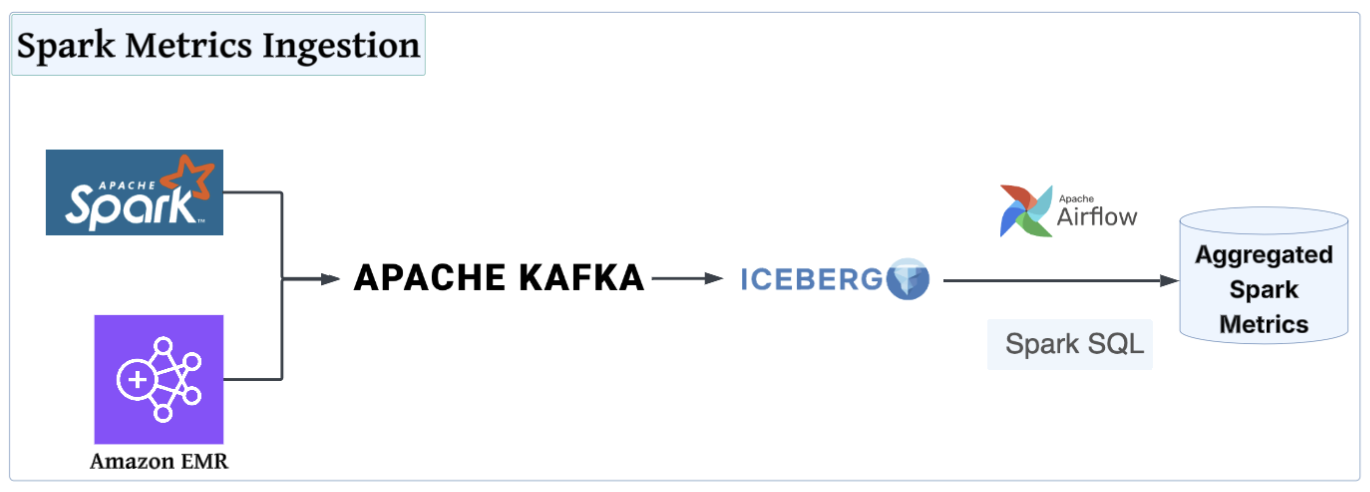
To address the challenges of managing Spark at scale, we developed a custom monitoring and optimization pipeline—from metric collection to AI-assisted tuning. It begins with our in-house Spark listener framework, which captures over 40 metrics in real time across Spark applications, jobs, stages, and tasks while pulling critical operational context from tools such as Apache Airflow and Apache Hadoop YARN.

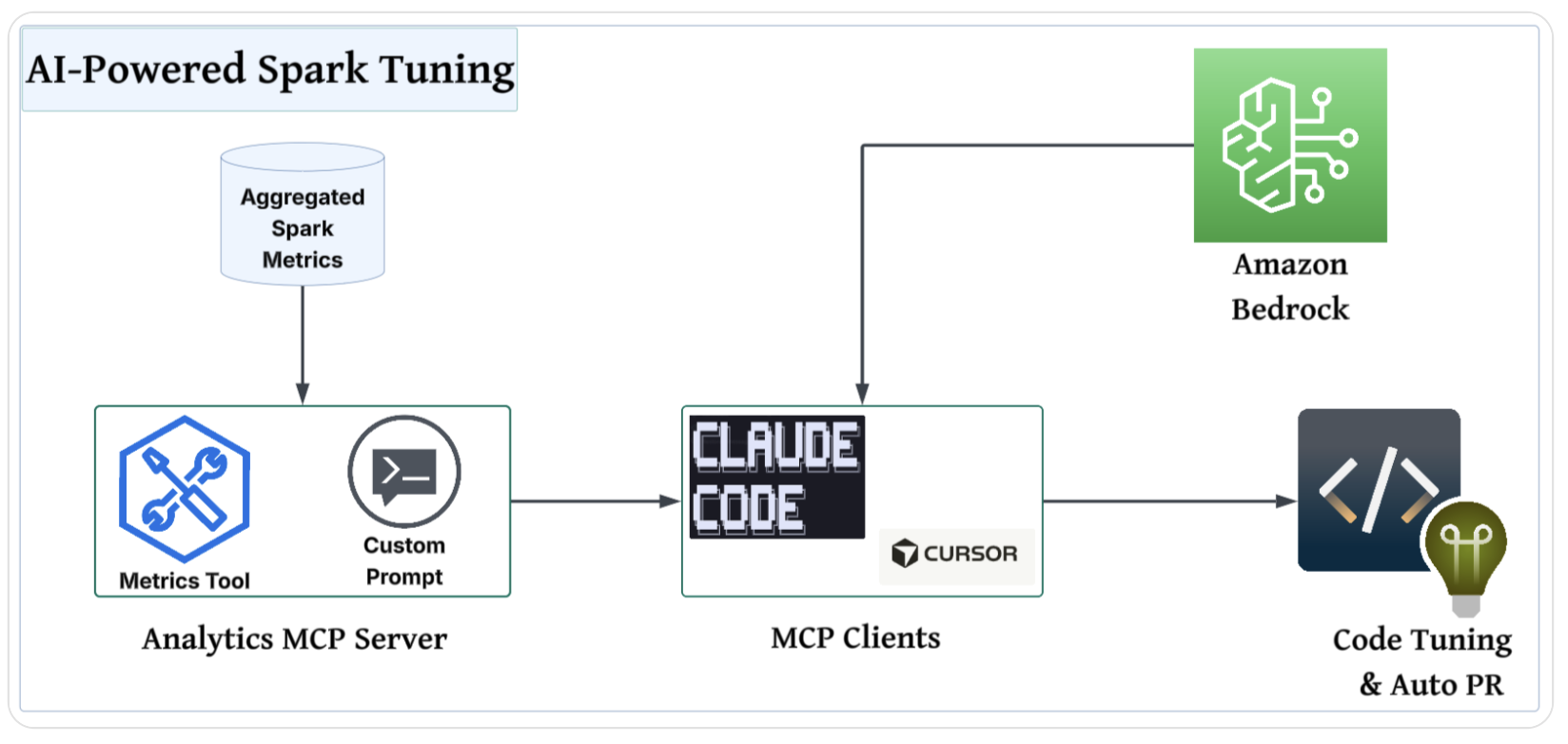
An Apache Airflow-orchestrated Spark SQL pipeline transforms this data into actionable insights, surfacing performance bottlenecks and failure points. To integrate these metrics into the developer tuning workflow, we expose a metrics tool and a custom prompt through our internal analytics model context protocol (MCP) server. This enables seamless integration with AI-assisted coding tools such as Cursor or Claude Code.

The following is the list of tools used for our Spark monitoring solution, which includes metric collection to AI-assisted tuning:

The result is fast, reliable, deterministic Spark tuning without the guesswork. Developers get environment-aware recommendations, automated configuration updates, and ready-to-review pull requests.

Deep dive into Spark metrics collection

At the center of our real-time monitoring solution lies a custom Spark listener framework that captures thorough telemetry across the Spark lifecycle. Spark’s built-in metrics are often coarse, short‑lived, and scattered across the user interface (UI) and logs, which leaves four critical gaps:

  1. Consistent historical record
  2. Weak linkage from applications to jobs to stages to tasks
  3. Limited context (user, cluster, team)
  4. Poor visibility into patterns such as skew, spill, and retries

Our expanded listener framework closes these gaps by unifying and enriching telemetry with environment and configuration tags, building a durable, queryable history, and correlating events across the execution graph. It explains why tasks fail, pinpoints where memory or CPU pressure occurs, compares intended configurations to actual usage, and produces clear, repeatable tuning recommendations so teams can baseline behavior, minimize waste, and resolve issues faster. The following architecture diagram illustrates the flow of the Spark metrics collection pipeline.

Spark metrics ingestion architecture diagram

Spark listener

Our listener framework captures Spark metrics at four distinct levels:

  1. Application metrics: Overall application success/failure rates, total runtime, and resource allocation
  2. Job-level metrics: Individual job duration and status tracking within an application
  3. Stage-level metrics: Stage execution details, shuffle operations, and memory usage per stage
  4. Task-level metrics: Individual task performance for deep debugging scenarios

The following Scala example code shows the SparkTaskListener extends the class SparkListener to capture detailed task-level metrics:

class SparkTaskListener(conf: SparkConf) extends SparkListener {
 val taskToStageId = new mutable.HashMap[Long, Int]()
 val stageToJobID = new mutable.HashMap[Int, Int]()
 private val emitter: Emitter = getEmitter(conf)
  override def onTaskStart(taskStart: SparkListenerTaskStart): Unit = {
   taskToStageId += taskStart.taskInfo.taskId -> taskStart.stageId 
 }
 override def onTaskEnd(taskEnd: SparkListenerTaskEnd): Unit = {
   val taskInfo = taskEnd.taskInfo
   val taskMetrics = taskEnd.taskMetrics
   val jobId = stageToJobID.apply(taskToStageId.apply(taskInfo.taskId))
   val metrics = Map[String, Any](
     "event_type" -> "task_metric",
     "job_id" -> jobId,
     "task_id" -> taskInfo.taskId,
     "duration" -> taskInfo.duration,
     "executor_run_time" -> taskMetrics.executorRunTime,
     "memory_bytes_spilled" -> taskMetrics.memoryBytesSpilled,
     "bytes_read" -> taskMetrics.inputMetrics.bytesRead,
     "records_read" -> taskMetrics.inputMetrics.recordsRead
     // additional metrics.....
   )
   emitter.report(convertToJson(metrics))
 }
}

Real-time streaming to Kafka

These metrics are streamed in real time to Kafka as JSON-formatted telemetry using a flexible emitter system:

class KafkaEmitter(conf: SparkConf) extends Emitter {
     private val broker = conf.get("spark.custom.listener.kafkaBroker", "<broker_address>")
     private val topic = conf.get("spark.custom.listener.kafkaTopic", "<topic_name>")
     private var producer: Producer[String, Array[Byte]] = _
     override def report(str: String): Unit = {
         val message = str.getBytes(StandardCharsets.UTF_8)
         producer.send(new ProducerRecord[String, Array[Byte]](topic, message))
     }
}

From Kafka, a downstream pipeline ingests these records into an Apache Iceberg table.

Context-rich observability

Beyond standard Spark metrics, our framework captures essential operational context:

  • Airflow integration: DAG metadata, task IDs, and execution timestamps
  • Resource tracking: Configurable executor metrics (heap usage, execution memory)
  • Environment context: Cluster identification, user tracking, and Spark configurations
  • Failure analysis: Detailed error messages and task failure root causes

The combination of thorough metrics collection and real-time streaming has redefined Spark monitoring at scale, laying the groundwork for powerful insights.

Deep dive into Spark metrics processing

When raw metrics—often containing millions of records—are ingested from various sources, a Spark SQL pipeline transforms this high-volume data into actionable insights. It aggregates the data into a single row per application ID, significantly reducing complexity while preserving key performance signals.

For consistency in how teams interpret and act on this data, we apply the Five Pillars of Spark Monitoring, a structured framework that turns raw telemetry into clear diagnostics and repeatable optimization strategies, as shown in the following table.

Pillar Metrics Key purpose/insight Driving event
Application metadata and orchestration details
  • YARN metadata (app, attempt, allocated memory, compute cluster, final job status, run duration)
  • Airflow metadata (DAG, task, owner)
Correlate performance patterns with teams and infrastructure to identify inefficiencies and ownership.
  • Airflow metadata
  • YARN metadata on Amazon EMR on EC2
User-specified configuration
  • Given memory (driver, executor)
  • Dynamic allocation (min/max/initial executor count)
  • Cores per executor
  • Shuffle partitions
Compare configuration as opposed to actual performance to detect over- and under-provisioning and optimizing costs. This is where significant cost savings often hide. Spark event:

  • app_metric
Performance insights
  • Maximum skew ratio (75th percentile as opposed to max shuffle_total_bytes_read by Spark tasks per stage)
  • Total spill
  • Spark stage/task retry/failure
This is where the real diagnostic power lies. These metrics identify the three primary stoppers of Spark performance: skew, spill, and failures. Spark event:

  • task_metric
  • stage_metric
Execution insights
  • Spark job/stage/task count
  • Spark job/stage/task duration
Understand runtime distribution, identify bottlenecks, and highlight execution outliers. Spark event:

  • task_metric
  • stage_metric
  • job_metric
Resource usage and system health
  • Peak JVM heap memory
  • Max GC overhead %
Reveal memory inefficiencies and JVM-related pressure for cost and stability improvements. Comparing these against given configs helps identify waste and optimize resources. Spark event:

  • task_metric
  • stage_metric
  • executor_metric

AI-powered Spark tuning

The following architecture diagram illustrates the use of agentic AI tools to analyze the aggregated Spark metrics.

AI-powered Spark tuning diagram

To integrate these metrics into a developer’s tuning workflow, we build a custom Spark metrics tool and a custom prompt that any agent can use. We use our existing analytics service, a homegrown web application that users can query our data warehouse with, build dashboards, and share insights. The backend is written in Python using FastAPI, and we expose an MCP server from the same service by using FastMCP. By exposing the Spark metrics tool and custom prompt through the MCP server, we make it possible for developers to connect their preferred assisted coding tools (Cursor, Claude Code, and more) and use data to guide their tuning.

Because the data exposed by the analytics MCP server might be sensitive, we use Amazon Bedrock in our Amazon Web Services (AWS) account to provide the foundation models to our MCP clients. This keeps our data more secure and facilitates compliance because it never leaves our AWS environment.

Custom prompt

To create our custom prompt for AI-driven Spark tuning, we design a structured, rule-based format that encourages more deterministic and standardized output. The prompt defines the required sections (application overview, current Spark configuration, job health summary, resource recommendations, and summary) for consistency across analyses. We include detailed formatting rules, such as wrapping values in backticks, avoiding line breaks, and enforcing strict table structures to maintain clarity and machine readability. The prompt also embeds explicit guidance for interpreting Spark metrics and mapping them to recommended tuning actions based on best practices, with clear criteria for status flags and impact explanations. The prompt means that the AI’s recommendations can be traced, reproduced, and actioned based on the provided data by tightly controlling the input-output flow and attempting to prevent hallucinations.

Final results

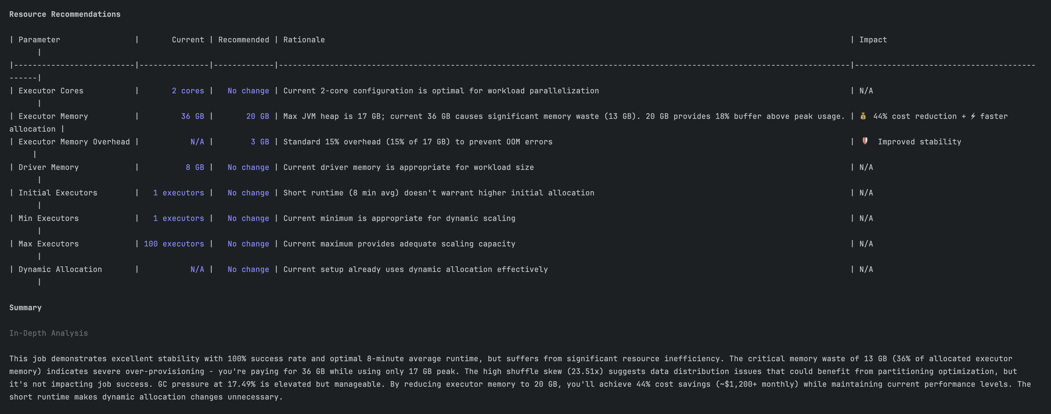
The screenshots in this section show how our tool performed the analysis and provided recommendations. The following is a performance analysis for an existing application.

performance analysis for an existing application

The following is a recommendation to reduce resource waste.

recommendation to reduce resource waste

The impact

Our AI-powered framework has fundamentally changed how Spark is monitored and managed at Slack. We’ve transformed Spark tuning from a high-expertise, trial-and-error process into an automated, data-backed standard by moving beyond traditional log-diving and embracing a structured, AI-driven approach. The results speak for themselves, as shown in the following table.

Metric Before After Improvement
Compute cost Non-deterministic Optimized resource use Up to 50% lower
Job completion time Non-deterministic Optimized Over 40% faster
Developer time on tuning Hours per week Minutes per week >90% reduction
Configuration waste Frequent over-provisioning Precise resource allocation Near-zero waste

Conclusion

At Slack, our experience with Spark monitoring shows that you don’t need to be a performance expert to achieve exceptional results. We’ve shifted from reacting to performance issues to preventing them by systematically applying five key metric categories.

The numbers speak for themselves: 30–50% cost reductions and 40–60% faster job completion times represent operational efficiency that directly impacts our ability to serve millions of users worldwide. These improvements compound over time as teams build confidence in their data infrastructure and can focus on innovation rather than troubleshooting.

Your organization can achieve similar outcomes. Start with the basics: implement comprehensive monitoring, establish baseline metrics, and commit to continuous optimization. Spark performance doesn’t require expertise in every parameter, but it does require a strong monitoring foundation and a disciplined approach to analysis.

Acknowledgments

We want to give our thanks to all the people who have contributed to this incredible journey: Johnny Cao, Nav Shergill, Yi Chen, Lakshmi Mohan, Apun Hiran, and Ricardo Bion.


About the authors

Nilanjana Mukherjee

Nilanjana Mukherjee

Nilanjana is a staff software engineer at Slack, bringing deep technical expertise and engineering leadership to complex software challenges. She specializes in building high-performance data systems, focusing on data pipeline architecture, query optimization, and scalable data processing solutions.

Tayven Taylor

Tayven Taylor

Tayven is a software engineer I on Slack’s Data Foundations team, where he helps maintain and optimize large-scale data systems. His work focuses on Spark and Amazon EMR performance, cost optimization, and reliability improvements that keep Slack’s data platform efficient and scalable. He’s passionate about creating tools and systems that make working with data faster, smarter, and more cost-effective.

Mimi Wang

Mimi Wang

Mimi is a staff software engineer on Slack’s Data Platform team, where she builds tools to facilitate data-driven decision-making at Slack. Recently she has been focusing on using AI to lower the barrier to entry for non-technical users to derive value out of data. Previously, she was on the Slack Security team focusing on a customer-facing real-time anomaly detection pipeline.

Rahul Gidwani

Rahul Gidwani

Rahul is a senior staff software engineer at Salesforce specializing in search infrastructure. He works on Slack’s data lake development and processing pipelines and contributing to open-source projects such as Apache HBase and Druid. Outside of work, Rahul enjoys rock climbing.

Prateek Kakirwar

Prateek Kakirwar

Prateek is a senior engineering manager at Slack leading the AI-first transformation of data engineering and analytics. With over 20 years of experience building large-scale data platforms, AI systems, and metrics frameworks, he focuses on scalable architectures that enable trusted, self-service analytics across the organization. He holds a master’s degree from the University of California, Berkeley.

Avijit Goswami

Avijit Goswami

Avijit is a principal specialist solutions architect at AWS specializing in data and analytics. He helps customers design and implement robust data lake solutions. Outside the office, you can find Avijit exploring new trails, discovering new destinations, cheering on his favorite teams, enjoying music, or testing out new recipes in the kitchen.

AWS analytics at re:Invent 2025: Unifying Data, AI, and governance at scale

Post Syndicated from Larry Weber original https://aws.amazon.com/blogs/big-data/aws-analytics-at-reinvent-2025-unifying-data-ai-and-governance-at-scale/

re:Invent 2025 showcased the bold Amazon Web Services (AWS) vision for the future of analytics, one where data warehouses, data lakes, and AI development converge into a seamless, open, intelligent platform, with Apache Iceberg compatibility at its core. Across over 18 major announcements spanning three weeks, AWS demonstrated how organizations can break down data silos, accelerate insights with AI, and maintain robust governance without sacrificing agility.

Amazon SageMaker: Your data platform, simplified

AWS introduced a faster, simpler approach to data platform onboarding for Amazon SageMaker Unified Studio. The new one-click onboarding experience eliminates weeks of setup, so teams can start working with existing datasets in minutes using their current AWS Identity and Access Management (IAM) roles and permissions. Accessible directly from Amazon SageMaker, Amazon Athena, Amazon Redshift, and Amazon S3 Tables consoles, this streamlined experience automatically creates SageMaker Unified Studio projects with existing data permissions intact. At its core is a powerful new serverless notebook that reimagines how data professionals work. This single interface combines SQL queries, Python code, Apache Spark processing, and natural language prompts, backed by Amazon Athena for Apache Spark to scale from interactive exploration to petabyte-scale jobs. Data engineers, analysts, and data scientists no longer need to context-switch between different tools based on workload—they can explore data with SQL, build models with Python, and use AI assistance, all in one place.

The introduction of Amazon SageMaker Data Agent in the new SageMaker notebooks marks a pivotal moment in AI-assisted development for data builders. This built-in agent doesn’t only generate code, it understands your data context, catalog information, and business metadata to create intelligent execution plans from natural language descriptions. When you describe an objective, the agent breaks down complex analytics and machine learning (ML) tasks into manageable steps, generates the required SQL and Python code, and maintains awareness of your notebook environment throughout the entire process. This capability transforms hours of manual coding into minutes of guided development, which means teams can focus on gleaning insights rather than repetitive boilerplate.

Embracing open data with Apache Iceberg

One significant theme across this year’s launches was the widespread adoption of Apache Iceberg across AWS analytics, transforming how organizations manage petabyte-scale data lakes. Catalog federation to remote Iceberg catalogs through the AWS Glue Data Catalog addresses a critical challenge in modern data architectures. You can now query remote Iceberg tables, stored in Amazon Simple Storage Service (Amazon S3) and catalogued in remote Iceberg catalogs, using preferred AWS analytics services such as Amazon Redshift, Amazon EMR, Amazon Athena, AWS Glue, and Amazon SageMaker, without moving or copying tables. Metadata synchronizes in real time, providing query results that reflect the current state. Catalog federation supports both coarse-grained access control and fine-grained access permissions through AWS Lake Formation enabling cross-account sharing and trusted identity propagation while maintaining consistent security across federated catalogs.

Amazon Redshift now writes directly to Apache Iceberg tables, enabling true open lakehouse architectures where analytics seamlessly span data warehouses and lakes. Apache Spark on Amazon EMR 7.12, AWS Glue, Amazon SageMaker notebooks, Amazon S3 Tables, and the AWS Glue Data Catalog now support Iceberg V3’s capabilities, including deletion vectors that mark deleted rows without expensive file rewrites, dramatically reducing pipeline costs and accelerating data modifications and row lineage. V3 automatically tracks every record’s history, creating audit trails essential for compliance and has table-level encryption that helps organizations meet stringent privacy regulations. These innovations mean faster writes, lower storage costs, comprehensive audit trails, and efficient incremental processing across your data architecture.

Governance that scales with your organization

Data governance received substantial attention at re:Invent with major enhancements to Amazon SageMaker Catalog. Organizations can now curate data at the column level with custom metadata forms and rich text descriptions, indexed in real time for immediate discoverability. New metadata enforcement rules require data producers to classify assets with approved business vocabulary before publication, providing consistency across the enterprise. The catalog uses Amazon Bedrock large language models (LLMs) to automatically suggest relevant business glossary terms by analyzing table metadata and schema information, bridging the gap between technical schemas and business language. Perhaps most importantly, SageMaker Catalog now exports its entire asset metadata as queryable Apache Iceberg tables through Amazon S3 Tables. This way, teams can analyze catalog inventory with standard SQL to answer questions like “which assets lack business descriptions?” or “how many confidential datasets were registered last month?” without building custom ETL infrastructure.

As organizations adopt multi-warehouse architectures to scale and isolate workloads, the new Amazon Redshift federated permissions capability eliminates governance complexity. Define data permissions one time from a Amazon Redshift warehouse, and they automatically enforce them across the warehouses in your account. Row-level, column-level, and masking controls apply consistently regardless of which warehouse queries originate from, and new warehouses automatically inherit permission policies. This horizontal scalability means organizations can add warehouses without increasing governance overhead, and analysts immediately see the databases from registered warehouses.

Accelerating AI innovation with Amazon OpenSearch Service

Amazon OpenSearch Service introduced powerful new capabilities to simplify and accelerate AI application development. With support for OpenSearch 3.3, agentic search enables precise results using natural language inputs without the need for complex queries, making it easier to build intelligent AI agents. The new Apache Calcite-powered PPL engine delivers query optimization and an extensive library of commands for more efficient data processing.

As seen in Matt Garman’s keynote, building large-scale vector databases is now dramatically faster with GPU acceleration and auto-optimization. Previously, creating large-scale vector indexes required days of building time and weeks of manual tuning by experts, which slowed innovation and prevented cost-performance optimizations. The new serverless auto-optimize jobs automatically evaluate index configurations—including k-nearest neighbors (k-NN) algorithms, quantization, and engine settings—based on your specified search latency and recall requirements. Combined with GPU acceleration, you can build optimized indexes up to ten times faster at 25% of the indexing cost, with serverless GPUs that activate dynamically and bill only when providing speed boosts. These advancements simplify scaling AI applications such as semantic search, recommendation engines, and agentic systems, so teams can innovate faster by dramatically reducing the time and effort needed to build large-scale, optimized vector databases.

Performance and cost optimization

Also announced in the keynote, Amazon EMR Serverless now eliminates local storage provisioning for Apache Spark workloads, introducing serverless storage that reduces data processing costs by up to 20% while preventing job failures from disk capacity constraints. The fully managed, auto scaling storage encrypts data in transit and at rest with job-level isolation, allowing Spark to release workers immediately when idle rather than keeping them active to preserve temporary data. Additionally, AWS Glue introduced materialized views based on Apache Iceberg, storing precomputed query results that automatically refresh as source data changes. Spark engines across Amazon Athena, Amazon EMR, and AWS Glue intelligently rewrite queries to use these views, accelerating performance by up to eight times while reducing compute costs. The service handles refresh schedules, change detection, incremental updates, and infrastructure management automatically.

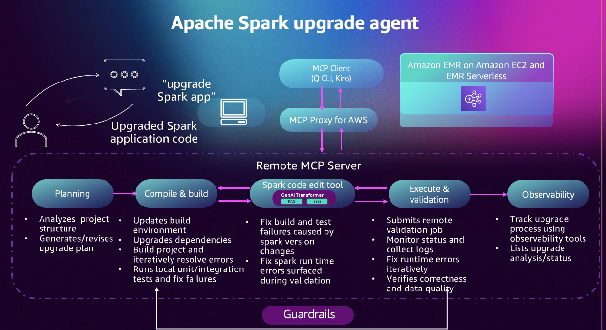
The new Apache Spark upgrade agent for Amazon EMR transforms version upgrades from months-long projects into week-long initiatives. Using conversational interfaces, engineers express upgrade requirements in natural language while the agent automatically identifies API changes and behavioral modifications across PySpark and Scala applications. Engineers review and approve suggested changes before implementation, maintaining full control while the agent validates functional correctness through data quality checks. Currently supporting upgrades from Spark 2.4 to 3.5, this capability is available through SageMaker Unified Studio, Kiro CLI, or an integrated development environment (IDE) with Model Context Protocol compatibility.

For workflow optimization, AWS introduced a new Serverless deployment option for Amazon Managed Workflows for Apache Airflow (Amazon MWAA), which eliminates the operational overhead of managing Apache Airflow environments while optimizing costs through serverless scaling. This new offering addresses key challenges of operational scalability, cost optimization, and access management that data engineers and DevOps teams face when orchestrating workflows. With Amazon MWAA Serverless, data engineers can focus on defining their workflow logic rather than monitoring for provisioned capacity. They can now submit their Airflow workflows for execution on a schedule or on demand, paying only for the actual compute time used during each task’s execution.

Looking forward

These launches collectively represent more than incremental improvements. They signal a fundamental shift in how organizations are approaching analytics. By unifying data warehousing, data lakes, and ML under a common framework built on Apache Iceberg, simplifying access through intelligent interfaces powered by AI, and maintaining robust governance that scales effortlessly, AWS is giving organizations the tools to focus on insights rather than infrastructure. The emphasis on automation, from AI-assisted development to self-managing materialized views and serverless storage, reduces operational overhead while improving performance and cost efficiency. As data volumes continue to grow and AI becomes increasingly central to business operations, these capabilities position AWS customers to accelerate their data-driven initiatives with unprecedented simplicity and power. To view the Re:Invent 2025 Innovation Talk on analytics, visit Harnessing analytics for humans and AI on YouTube.


About the authors

Larry Weber

Larry Weber

Larry leads product marketing for the analytics portfolio at AWS.

Amazon EMR Serverless eliminates local storage provisioning, reducing data processing costs by up to 20%

Post Syndicated from Karthik Prabhakar original https://aws.amazon.com/blogs/big-data/amazon-emr-serverless-eliminates-local-storage-provisioning-reducing-data-processing-costs-by-up-to-20/

At AWS re:Invent 2025, Amazon Web Services (AWS) announced serverless storage for Amazon EMR Serverless, a new capability that eliminates the need configure local disks for Apache Spark workloads. This reduces data processing costs by up to 20% while eliminating job failures from disk capacity constraints.

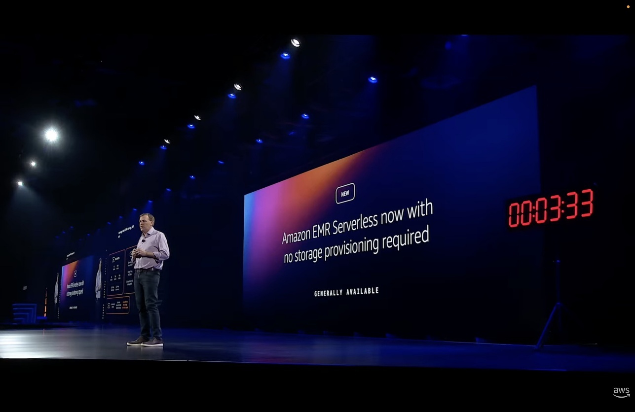
With serverless storage, Amazon EMR Serverless automatically handles intermediate data operations, such as shuffle, on your behalf. You pay only for compute and memory—no storage charges. By decoupling storage from compute, Spark can release idle workers immediately, reducing costs throughout the job lifecycle. The following image shows the serverless storage for EMR Serverless announcement from the AWS re:Invent 2025 keynote:

The challenge: Sizing local disk storage

Running Apache Spark workloads requires sizing local disk storage for shuffle operations—where Spark redistributes data across executors during joins, aggregations, and sorts. This requires analyzing job histories to estimate disk requirements, leading to two common problems: overprovisioning wastes money on unused capacity, and under provisioning causes job failures when disk space runs out. Most customers overprovision local storage to ensure jobs complete successfully in production.

Data skew compounds this further. When one executor handles a disproportionately large partition, that executor takes significantly longer to complete while other workers sit idle. If you didn’t provision enough disk for that skewed executor, the job fails entirely—making data skew one of the top causes of Spark job failures. However, the problem extends beyond capacity planning. Because shuffle data couples tightly to local disks, Spark executors pin to worker nodes even when compute requirements drop between job stages. This prevents Spark from releasing workers and scaling down, inflating compute costs throughout the job lifecycle. When a worker node fails, Spark must recompute the shuffle data stored on that node, causing delays and inefficient resource usage.

How it works

Serverless storage for Amazon EMR Serverless addresses these challenges by offloading shuffle operations from individual compute workers onto a separate, elastic storage layer. Instead of storing critical data on local disks attached to Spark executors, serverless storage automatically provisions and scales high-performance remote storage as your job runs.

The architecture provides several key benefits. First, compute and storage scale independently—Spark can acquire and release workers as needed across job stages without worrying about preserving locally stored data. Second, shuffle data is evenly distributed across the serverless storage layer, eliminating data skew bottlenecks that occur when some executors handle disproportionately large shuffle partitions. Third, if a worker node fails, your job continues processing without delays or reruns because data is reliably stored outside individual compute workers.

Serverless storage is provided at no additional charge, and it eliminates the cost associated with local storage. Instead of paying for fixed disk capacity sized for maximum potential I/O load—capacity that often sits idle during lighter workloads—you can use serverless storage without incurring storage costs. You can focus your budget on compute resources that directly process your data, not on managing and overprovisioning disk storage.

Technical innovation brings three breakthroughs

Serverless storage introduces three fundamental innovations that solve Spark’s shuffle bottlenecks: multi-tier aggregation architecture, purpose-built networking, and true storage-compute decoupling. Apache Spark’s shuffle mechanism has a core constraint: each mapper independently writes output as small files, and each reducer must fetch data from potentially thousands of workers. In a large-scale job with 10,000 mappers and 1,000 reducers, this creates 10 million individual data exchanges. Serverless storage aggregates early and intelligently—mappers stream data to an aggregation layer that consolidates shuffle data in memory before committing to storage. Whereas individual shuffle write and fetch operations might show slightly higher latency due to network round-trips compared to local disk I/O, the overall job performance improves by transforming millions of tiny I/O operations into a smaller number of large, sequential operations.

Traditional Spark shuffle creates a mesh network where each worker maintains connections to potentially hundreds of other workers, spending significant CPU on connection management rather than data processing. We built a custom networking stack where each mapper opens a single persistent remote procedure call (RPC) connection to our aggregator layer, eliminating the mesh complexity. Although individual shuffle operations might show slightly higher latency due to network round trips compared to local disk I/O, overall job performance improves through better resource utilization and elastic scaling. Workers no longer run a shuffle service—they focus entirely on processing your data.

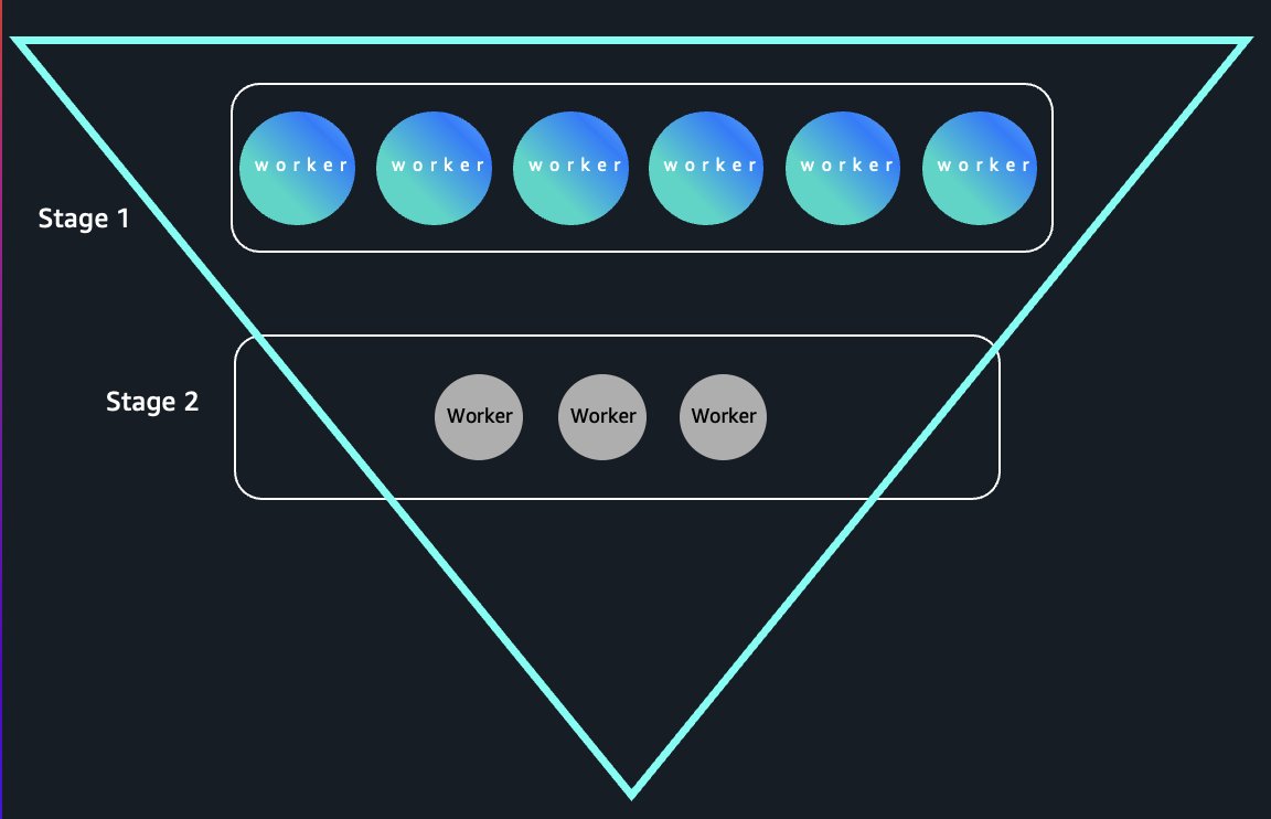
Traditional Amazon EMR Serverless jobs store shuffle data on local disks, coupling data lifecycle to worker lifecycle—idle workers can’t terminate without losing shuffle data. Serverless storage decouples these entirely by storing shuffle data in AWS managed storage with opaque handles tracked by the driver. Workers can terminate immediately after completing tasks without data loss, enabling elastic scaling. In funnel-shaped queries where early stages require massive parallelism that narrows as data aggregates, we’re seeing up to 80% compute cost reduction in benchmarks by releasing idle workers instantly. The following diagram illustrates instant worker release in funnel-shaped queries.

Our aggregator layer integrates directly with AWS Identity and Access Management (IAM), AWS Lake Formation, and fine-grained access control systems, providing job-level data isolation with access controls that match source data permissions.

Getting started

Serverless storage is available in multiple AWS Regions. For the current list of supported Regions, refer to the Amazon EMR User Guide.

New applications

Serverless storage can be enabled for new applications starting with Amazon EMR release 7.12. Follow these steps:

  1. Create an Amazon EMR Serverless application with Amazon EMR 7.12 or later:
aws emr-serverless create-application \
  --type "SPARK" \
  --name my-application \
  --release-label emr-7.12.0 \
  --runtime-configuration '[{
      "classification": "spark-defaults",
        "properties": {
          "spark.aws.serverlessStorage.enabled": "true"
        }
    }]' \
  --region us-east-1
  1. Submit your Spark job:
aws emr-serverless start-job-run \
  --application-id <application-id> \
  --execution-role-arn <execution-role-arn> \
  --job-driver '{
    "sparkSubmit": {
      "entryPoint": "s3://<bucket>/<your_script.py>",
      "sparkSubmitParameters": "--conf spark.executor.cores=4 --conf spark.executor.memory=20g --conf spark.driver.cores=4 --conf spark.driver.memory=8g --conf spark.executor.instances=10"
    }
  }'

Existing applications

You can enable serverless storage for existing applications on Amazon EMR 7.12 or later by updating your application settings.

To enable serverless storage using AWS Command Line Interface (AWS CLI), enter the following command:

aws emr-serverless update-application \
  --application-id <application-id> \
  --runtime-configuration '[{
      "classification": "spark-defaults",
        "properties": {
          "spark.aws.serverlessStorage.enabled": "true"
        }
    }]'

To enable serverless storage using Amazon EMR Studio UI, navigate to your application in Amazon EMR Studio, go to Configuration, and add the Spark property spark.aws.serverlessStorage.enabled=true in the spark-defaults classification.

Job-level configuration

You can also enable serverless storage for specific jobs, even when it’s not enabled at the application level:

aws emr-serverless start-job-run \
  --application-id <application-id> \
  --execution-role-arn <execution-role-arn> \
  --job-driver '{
    "sparkSubmit": {
      "entryPoint": "s3://<bucket>/<your_script.py>",
      "sparkSubmitParameters": "--conf spark.executor.cores=4 --conf spark.executor.memory=20g --conf spark.aws.serverlessStorage.enabled=true"
    }
  }'

(Optional) Disabling serverless storage

If you prefer to continue using local disks, you can disable serverless storage by omitting the spark.aws.serverlessStorage.enabled configuration or setting it to false at either the application or job level:

spark.aws.serverlessStorage.enabled=falseTo use traditional local disk provisioning, configure the appropriate disk type and size for your application workers.

Monitoring and cost tracking

You can monitor elastic shuffle usage through standard Spark UI metrics and track costs at the application level in AWS Cost Explorer and AWS Cost and Usage Reports. The service automatically handles performance optimization and scaling, so you don’t need to tune configuration parameters.

When to use serverless storage

Serverless storage delivers the most value for workloads with substantial shuffle operations—typically jobs that shuffle more than 10 GB of data (and less than 200 G per job, the limitation as of this writing). These include:

  • Large-scale data processing with heavy aggregations and joins
  • Sort-heavy analytics workloads
  • Iterative algorithms that repeatedly access the same datasets

Jobs with unpredictable shuffle sizes benefit particularly well because serverless storage automatically scales capacity up and down based on real-time demand. For workloads with minimal shuffle activity or very short duration (under 2–3 minutes), the benefits might be limited. In these cases, the overhead of remote storage access might outweigh the advantages of elastic scaling.

Security and data lifecycle

Your data is stored in serverless storage only while your job is running and is automatically deleted when your job is completed. Because Amazon EMR Serverless batch jobs can run for up to 24 hours, your data will be stored for no longer than this maximum duration. Serverless storage encrypts your data both in transit between your Amazon EMR Serverless application and the serverless storage layer and at rest while temporarily stored, using AWS managed encryption keys. The service uses an IAM based security model with job-level data isolation, which means that one job can’t access the shuffle data of another job. Serverless storage maintains the same security standards as Amazon EMR Serverless, with enterprise-grade security controls throughout the processing lifecycle.

Conclusion

Serverless storage represents a fundamental shift in how we approach data processing infrastructure, eliminating manual configuration, aligning costs to actual usage, and improving reliability for I/O intensive workloads. By offloading shuffle operations to a managed service, data engineers can focus on building analytics rather than managing storage infrastructure.

To learn more about serverless storage and get started, visit the Amazon EMR Serverless documentation.


About the authors

Karthik Prabhakar

Karthik Prabhakar

Karthik is a Data Processing Engines Architect for Amazon EMR at AWS. He specializes in distributed systems architecture and query optimization, working with customers to solve complex performance challenges in large-scale data processing workloads. His focus spans engine internals, cost optimization strategies, and architectural patterns that enable customers to run petabyte-scale analytics efficiently.

Ravi Kumar

Ravi Kumar

Ravi is a Senior Product Manager Technical at Amazon Web Services, specializing in exabyte-scale data infrastructure and analytics platforms. He helps customers unlock insights from structured and unstructured data using open-source technologies and cloud computing. Outside of work, Ravi enjoys exploring emerging trends in data science and machine learning.

Matt Tolton

Matt Tolton

Matt is a Senior Principal Engineer at Amazon Web Services.

author name

Neil Mukerje

Neil is a Principal Product Manager at Amazon Web Services.

Modernize Apache Spark workflows using Spark Connect on Amazon EMR on Amazon EC2

Post Syndicated from Philippe Wanner original https://aws.amazon.com/blogs/big-data/modernize-apache-spark-workflows-using-spark-connect-on-amazon-emr-on-amazon-ec2/

Apache Spark Connect, introduced in Spark 3.4, enhances the Spark ecosystem by offering a client-server architecture that separates the Spark runtime from the client application. Spark Connect enables more flexible and efficient interactions with Spark clusters, particularly in scenarios where direct access to cluster resources is limited or impractical.

A key use case for Spark Connect on Amazon EMR is to be able to connect directly from your local development environments to Amazon EMR clusters. By using this decoupled approach, you can write and test Spark code on your laptop while using Amazon EMR clusters for execution. This capability reduces development time and simplifies data processing with Spark on Amazon EMR.

In this post, we demonstrate how to implement Apache Spark Connect on Amazon EMR on Amazon Elastic Compute Cloud (Amazon EC2) to build decoupled data processing applications. We show how to set up and configure Spark Connect securely, so you can develop and test Spark applications locally while executing them on remote Amazon EMR clusters.

Solution architecture

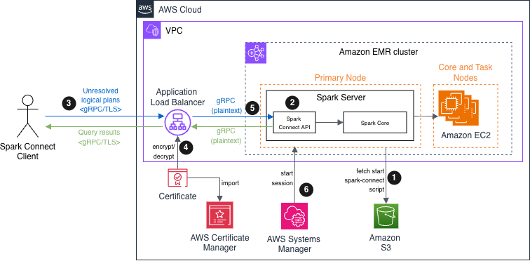
The architecture centers on an Amazon EMR cluster with two node types. The primary node hosts both the Spark Connect API endpoint and Spark Core components, serving as the gateway for client connections. The core node provides additional compute capacity for distributed processing. Although this solution demonstrates the architecture with two nodes for simplicity, it scales to support multiple core and task nodes based on workload requirements.

In Apache Spark Connect version 4.x, TLS/SSL network encryption is not inherently supported. We show you how to implement secure communications by deploying an Amazon EMR cluster with Spark Connect on Amazon EC2 using an Application Load Balancer (ALB) with TLS termination as the secure interface. This approach enables encrypted data transmission between Spark Connect clients and Amazon Virtual Private Cloud (Amazon VPC) resources.

The operational flow is as follows:

  1. Bootstrap script – During Amazon EMR initialization, the primary node fetches and executes the start-spark-connect.sh file from Amazon Simple Storage Service (Amazon S3). This script starts the Spark Connect server.
  2. Server availability – When the bootstrap process is complete, the Spark Server enters a waiting state, ready to accept incoming connections. The Spark Connect API endpoint becomes available on the configured port (typically 15002), listening for gRPC connection from remote clients.
  3. Client interaction – Spark Connect clients can establish secure connections to an Application Load Balancer. These clients translate DataFrame operations into unresolved logical query plans, encode these plans using protocol buffers, and send them to the Spark Connect API using gRPC.
  4. Encryption in transit – The Application Load Balancer receives incoming gRPC or HTTPS traffic, performs TLS termination (decrypting the traffic), and forwards the requests to the primary node. The certificate is stored in AWS Certificate Manager (ACM).
  5. Request processing – The Spark Connect API receives the unresolved logical plans, translates them into Spark’s built-in logical plan operators, passes them to Spark Core for optimization and execution, and streams results back to the client as Apache Arrow-encoded row batches.
  6. (Optional) Operational access – Administrators can securely connect to both primary and core nodes through Session Manager, a capability of AWS Systems Manager, enabling troubleshooting and maintenance without exposing SSH ports or managing key pairs.

The following diagram depicts the architecture of this post’s demonstration for submitting Spark unresolved logical plans to EMR clusters using Spark Connect.

Apache Spark Connect on Amazon EMR solution architecture diagram

Apache Spark Connect on Amazon EMR solution architecture diagram

Prerequisites

To proceed with this post, ensure you have the following:

Implementation steps

In this recipe, through AWS CLI commands, you will:

  1. Prepare the bootstrap script, a bash script starting Spark Connect on Amazon EMR.
  2. Set up the permissions for Amazon EMR to provision resources and perform service-level actions with other AWS services.
  3. Create the Amazon EMR cluster with these associated roles and permissions and eventually attach the prepared script as a bootstrap action.
  4. Deploy the Application Load Balancer and certificate with ACM secure data in transit over the internet.
  5. Modify the primary node’s security group to allow Spark Connect clients to connect.
  6. Connect with a test application connecting the client to Spark Connect server.

Prepare the bootstrap script

To prepare the bootstrap script, follow these steps:

  1. Create an Amazon S3 bucket to host the bootstrap bash script:
    REGION=
    BUCKET_NAME=
    aws s3api create-bucket \
       --bucket $BUCKET_NAME \ 
       --region $REGION \
       --create-bucket-configuration LocationConstraint=$REGION

  2. Open your preferred text editor, add the following commands in a new file with a name such start-spark-connect.sh. If the script runs on the primary node, it starts Spark Connect server. If it runs on a task or core node, it does nothing:
    #!/bin/bash
    if grep isMaster /mnt/var/lib/info/instance.json | grep false;
    then
        echo "This is not master node, do nothing."
        exit 0
    fi
    echo "This is master, continuing to execute script"
    SPARK_HOME=/usr/lib/spark
    SPARK_VERSION=$(spark-submit --version 2>&1 | grep "version" | head -1 | awk '{print $NF}' | grep -oE '[0-9]+\.[0-9]+\.[0-9]+')
    SCALA_VERSION=$(spark-submit --version 2>&1 | grep -o "Scala version [0-9.]*" | awk '{print $3}' | grep -oE '[0-9]+\.[0-9]+')
    echo "Spark version ${SPARK_VERSION} is installed under ${SPARK_HOME} running with scala version ${SCALA_VERSION}"
    sudo "${SPARK_HOME}"/sbin/start-connect-server.sh --packages org.apache.spark:spark-connect_"${SCALA_VERSION}:${SPARK_VERSION}"

  3. Upload the script into the bucket created in step 1:
    aws s3 cp start-spark-connect.sh s3://$BUCKET_NAME
    

Set up the permissions

Before creating the cluster, you must create the service role, and instance profile. A service role is an IAM role that Amazon EMR assumes to provision resources and perform service-level actions with other AWS services. An EC2 instance profile for Amazon EMR assigns a role to every EC2 instance in a cluster. The instance profile must specify a role that can access the resources for your bootstrap action.

  1. Create the IAM role:
    aws iam create-role \
    --role-name AmazonEMR-ServiceRole-SparkConnectDemo \
    --assume-role-policy-document '{
    	"Version": "2012-10-17",
    	"Statement": [{
    		"Effect": "Allow",
    		"Principal": {"Service": "elasticmapreduce.amazonaws.com"},
    		"Action": "sts:AssumeRole"
    		}]
    }'
    

  2. Attach the necessary managed policies to the service role to allow Amazon EMR to manage the underlying services Amazon EC2 and Amazon S3 on your behalf and optionally grant an instance to interact with Systems Manager:
    aws iam attach-role-policy \
    --role-name AmazonEMR-ServiceRole-SparkConnectDemo \
    --policy-arn arn:aws:iam::aws:policy/service-role/AmazonEMRServicePolicy_v2
    
    aws iam attach-role-policy \
    --role-name AmazonEMR-ServiceRole-SparkConnectDemo \
    --policy-arn arn:aws:iam::aws:policy/AmazonSSMManagedInstanceCore
    
    aws iam attach-role-policy \
    --role-name AmazonEMR-ServiceRole-SparkConnectDemo \
    --policy-arn arn:aws:iam::aws:policy/service-role/AmazonElasticMapReduceRole
    

  3. Create an Amazon EMR instance role to grant permissions to EC2 instances to interact with Amazon S3 or other AWS services:
    aws iam create-role \
    --role-name EMR_EC2_SparkClusterNodesRole \
    --assume-role-policy-document '{
    "Version": "2012-10-17",
    "Statement": [{
       "Effect": "Allow",
       "Principal": {"Service": "ec2.amazonaws.com"},
       "Action": "sts:AssumeRole"
       }]
    }'
    

  4. To allow the primary instance to read from Amazon S3, attach the AmazonS3ReadOnlyAccess policy to the Amazon EMR instance role. For production environments, this access policy should be reviewed and replaced with a custom policy following the principle of least privilege, granting only the specific permissions needed for your use case:
    aws iam attach-role-policy \
    --role-name EMR_EC2_SparkClusterNodesRole \
    --policy-arn arn:aws:iam::aws:policy/AmazonS3ReadOnlyAccess
    

  5. Attaching AmazonSSMManagedInstanceCore policy enables the instances to use core Systems Manager features, such as Session Manager, and Amazon CloudWatch:
    aws iam attach-role-policy \
    --role-name EMR_EC2_SparkClusterNodesRole \
    --policy-arn arn:aws:iam::aws:policy/AmazonSSMManagedInstanceCore
    

  6. To pass the EMR_EC2_SparkClusterInstanceProfile IAM role information to the EC2 instances when they start, create the Amazon EMR EC2 instance profile:
    aws iam create-instance-profile \
    --instance-profile-name EMR_EC2_SparkClusterInstanceProfile
    

  7. Attach the role EMR_EC2_SparkClusterNodesRole created in step 3 to the newly instance profile:
    aws iam add-role-to-instance-profile \
    --instance-profile-name EMR_EC2_SparkClusterInstanceProfile \
    --role-name EMR_EC2_SparkClusterNodesRole
    

Create the Amazon EMR cluster

To create the Amazon EMR cluster, follow these steps:

  1. Set the environment variables, where your EMR cluster and load-balancer must be deployed:
    VPC_ID=<vpc-emr-and-alb>
    EMR_PRI_SB_ID_1=<emr-private-subnet-id-az1>
    ALB_PUB_SB_ID_1=<alb-public-subnet-id-az1>
    ALB_PUB_SB_ID_2=<alb-public-subnet-id-az2>
    

  2. Create the EMR cluster with the latest Amazon EMR release. Replace the placeholder value with your actual S3 bucket name where the bootstrap action script is stored:
    CLUSTER_ID=$(aws emr create-cluster \
    --name "Spark Connect cluster demo" \
    --applications Name=Spark \
    --release-label emr-7.9.0 \
    --service-role AmazonEMR-ServiceRole-SparkConnectDemo \
    --ec2-attributes InstanceProfile=EMR_EC2_SparkClusterInstanceProfile,SubnetId=$EMR_PRI_SB_ID_1 \
    --instance-groups InstanceGroupType=MASTER,InstanceCount=1,InstanceType=m5.xlarge InstanceGroupType=CORE,InstanceCount=1,InstanceType=m5.xlarge \
    --bootstrap-actions Path="s3://$BUCKET_NAME/start-spark-connect.sh" \
    --query 'ClusterId' --output text)
    echo CLUSTER_ID="$CLUSTER_ID"
    

    To modify primary node’s security group to allow Systems Manager to start a session.

  3. Get the primary node’s security group identifier. Record the identifier because you’ll need it for subsequent configuration steps in which primary-node-security-group-id is mentioned:
    PRIMARY_NODE_SG=$(aws emr describe-cluster \
    --cluster-id $CLUSTER_ID \
    --query 'Cluster.Ec2InstanceAttributes.EmrManagedMasterSecurityGroup' \
    --output text)
    echo PRIMARY_NODE_SG=$PRIMARY_NODE_SG
    

  4. Find the EC2 instance connect prefix list ID for your Region. You can use the EC2_INSTANCE_CONNECT filter with the describe-managed-prefix-lists command. Using a managed prefix list provides a dynamic security configuration to authorize Systems Manager EC2 instances to connect the primary and core nodes by SSH:
    IC_PREFIX_LIST=$(aws ec2 describe-managed-prefix-lists \
    --filters Name=prefix-list-name,Values=com.amazonaws.$REGION.ec2-instance-connect \
    --query 'PrefixLists[0].PrefixListId' \
    --output text)
    echo IC_PREFIX_LIST=$IC_PREFIX_LIST
    

  5. Modify the primary node security group inbound rules to allow SSH access (port 22) to the EMR cluster’s primary node from resources that are part of the specified Instance Connect service contained in the prefix list:
    aws ec2 authorize-security-group-ingress \
    --region $REGION \
    --group-id $PRIMARY_NODE_SG \
    --ip-permissions "[{\"IpProtocol\":\"tcp\",\"FromPort\":22,\"ToPort\":22,\"PrefixListIds\":[{\"PrefixListId\":\"$IC_PREFIX_LIST\"}]}]"
    

Optionally, you can repeat the preceding steps 1–3 for the core (and tasks) cluster’s nodes to allow Amazon EC2 Instance Connect to access the EC2 instance through SSH.

Deploy the Application Load Balancer and certificate

To deploy the Application Load Balancer and certificate, follow these steps:

  1. Create a load balancer’s security group:
    ALB_SG_ID=$(aws ec2 create-security-group \
    --group-name spark-connect-alb-sg \
    --description "Security group for Spark Connect ALB" \
    --region $REGION \
    --vpc-id $VPC_ID \
    --query 'GroupId' \
    --output text)
    

  2. Add rule to accept TCP traffic from a trusted IP on port 443. We recommend that you use the local development machine’s IP address. You can check your current public IP address here: https://checkip.amazonaws.com:
    aws ec2 authorize-security-group-ingress \
    --group-id $ALB_SG_ID \
    --protocol tcp \
    --port 443 \
    --cidr <replace-with-trusted-IP>/32
    

  3. Create a new target group with gRPC protocol, which targets the Spark Connect server instance and the port the server is listening to:
    ALB_TG_ARN=$(aws elbv2 create-target-group \
    --name spark-connect-tg \
    --protocol HTTP \
    --protocol-version GRPC \
    --port 15002 \
    --target-type instance \
    --health-check-enabled \
    --health-check-protocol HTTP \
    --health-check-path / \
    --vpc-id $VPC_ID \
    --query 'TargetGroups[0].TargetGroupArn' \
    --output text)
    echo "ALB TG created (ARN)=$ALB_TG_ARN"
    

  4. Create the Application Load Balancer:
    ALB_ARN=$(aws elbv2 create-load-balancer \
    --name spark-connect-alb \
    --type application \
    --scheme internet-facing \
    --subnets $ALB_PUB_SB_ID_1 $ALB_PUB_SB_ID_2 \
    --security-groups $ALB_SG_ID \
    --query 'LoadBalancers[0].LoadBalancerArn' \
    --output text)
    echo "ALB created (ARN)=$ALB_ARN"
    

  5. Get the load balancer DNS name:
    ALB_DNS=$(aws elbv2 describe-load-balancers \
    --load-balancer-arns $ALB_ARN \
    --query 'LoadBalancers[0].DNSName' \
    --output text)
    echo "ALB DNS=$ALB_DNS"
    

  6. Retrieve the Amazon EMR primary node ID:
    PRIMARY_NODE_ID=$(aws emr list-instances --cluster-id $CLUSTER_ID --instance-group-types MASTER --query 'Instances[0].Ec2InstanceId' --output text)
    echo PRIMARY_NODE_ID=$PRIMARY_NODE_ID
    

  7. (Optional) To encrypt and decrypt the traffic, the load balancer needs a certificate. You can skip this step if you already have a trusted certificate in ACM. Otherwise, create a self-signed certificate:
    PRIVATE_KEY_PATH=./sc-private-key.key
    CERTIFICATE_PATH=./sc-certificate.cert
    sudo openssl req -x509 -nodes -days 365 -newkey rsa:2048 -keyout $PRIVATE_KEY_PATH -out $CERTIFICATE_PATH -subj "/CN=$ALB_DNS"
    

  8. Upload to ACM:
    ACM_CERT_ARN=$(aws acm import-certificate \
    --certificate fileb://$CERTIFICATE_PATH \
    --private-key fileb://$PRIVATE_KEY_PATH \
    --region $REGION \
    --query CertificateArn \
    --output text)
    echo "Certificate created (ARN)=$ACM_CERT_ARN"
    

  9. Create the load balancer listener:
    ALB_LISTENER_ARN=$(aws elbv2 create-listener \
    --load-balancer-arn $ALB_ARN \
    --protocol HTTPS \
    --port 443 \
    --certificates CertificateArn=$ACM_CERT_ARN \
    --ssl-policy ELBSecurityPolicy-TLS13-1-2-2021-06 \
    --default-actions Type=forward,TargetGroupArn=$ALB_TG_ARN \
    --region $REGION \
    --query 'Listeners[0].ListenerArn' \
    --output text)
    echo "ALB listener created (ARN)=$ALB_LISTENER_ARN"
    

  10. After the listener has been provisioned, register the primary node to the target group:
    aws elbv2 register-targets \
    --target-group-arn $ALB_TG_ARN \
    --targets Id=$PRIMARY_NODE_ID
    

Modify the primary node’s security group to allow Spark Connect clients to connect

To connect to Spark Connect, amend only the primary security group. Add an inbound rule to the primary’s node security group to accept Spark Connect TCP connection on port 15002 from your chosen trusted IP address:

aws ec2 authorize-security-group-ingress \
--group-id $PRIMARY_NODE_SG \
--protocol tcp \
--port 15002 \
--source-group $ALB_SG_ID

Connect with a test application

This example demonstrates that a client running a newer Spark version (4.0.1) can successfully connect to an older Spark version on the Amazon EMR cluster (3.5.5), showcasing Spark Connect’s version compatibility feature. This version combination is for demonstration only. Running older versions might pose security risks in production environments.

To test the client-to-server connection, we provide the following test Python application. We recommend that you create and activate a Python virtual environment (venv) before installing the packages. This helps isolate the dependencies for this specific project and prevents conflicts with other Python projects. To install packages, run the following command:

pip install pyspark-client==4.0.1

In your integrated development environment (IDE), copy and paste the following code, replace the placeholder, and invoke it. The code creates a Spark DataFrame containing two rows and it shows its data:

from pyspark.sql import SparkSession
import os
os.environ['GRPC_DEFAULT_SSL_ROOTS_FILE_PATH'] = os.path.expanduser('sc-certificate.cert')
spark = SparkSession.builder \
    .remote("sc://:443/;use_ssl=true") \
    .config('spark.sql.execution.pandas.inferPandasDictAsMap', True) \
    .config('spark.sql.pyspark.legacy.inferMapTypeFromFirstPair.enabled', True) \
    .getOrCreate()
spark.createDataFrame([("sue", 32),("li", 3)],["first_name", "age"]).show()

The following shows the application output:

+----------+---+
|first_name|age|
+----------+---+
|       sue| 32|
|        li|  3|
+----------+---+

Clean up

When you no longer need the cluster, release the following resources to stop incurring charges:

  1. Delete the Application Load Balancer listener, target group, and the load balancer.
  2. Delete the ACM certificate.
  3. Delete the load balancer and Amazon EMR node security groups.
  4. Terminate the EMR cluster.
  5. Empty the Amazon S3 bucket and delete it.
  6. Remove AmazonEMR-ServiceRole-SparkConnectDemo and EMR_EC2_SparkClusterNodesRole roles and EMR_EC2_SparkClusterInstanceProfile instance profile.

Considerations

Security considerations with Spark Connect:

  • Private subnet deployment – Keep EMR clusters in private subnets with no direct internet access, using NAT gateways for outbound connectivity only.
  • Access logging and monitoring – Enable VPC Flow Logs, AWS CloudTrail, and bastion host access logs for audit trails and security monitoring.
  • Security group restrictions – Configure security groups to allow Spark Connect port (15002) access only from bastion host or specific IP ranges.

Conclusion

In this post, we showed how you can adopt modern development workflows and debug Spark applications from local IDEs or notebooks, so you can step through code execution. With Spark Connect’s client-server architecture, the Spark cluster can run on a different version than the client applications, so operations teams can perform infrastructure upgrades and patches independently.

As the cluster operators gain experience, they can customize the bootstrap actions and add steps to process data. Consider exploring Amazon Managed Workflows for Apache Airflow (MWAA) for orchestrating your data pipeline.


About the authors

Philippe Wanner

Philippe Wanner

Philippe is EMEA Tech Lead at AWS. His role is to accelerate the digital transformation for large organizations. His current focus is in a multidisciplinary area involving business transformation, technical strategy, and distributed systems.

Ege Oguzman

Ege Oguzman

Ege is a Software Development Engineer at AWS, and previously he was a Solutions Architect in the public sector. As a builder and cloud enthusiast, he specializes in distributed systems and dedicates his time to infrastructure development and helping organizations build solutions on AWS.

Introducing the Apache Spark troubleshooting agent for Amazon EMR and AWS Glue

Post Syndicated from Jake Zych original https://aws.amazon.com/blogs/big-data/introducing-the-apache-spark-troubleshooting-agent-for-amazon-emr-and-aws-glue/

The newly launched Apache Spark troubleshooting agent can eliminate hours of manual investigation for data engineers and scientists working with Amazon EMR or AWS Glue. Instead of navigating multiple consoles, sifting through extensive log files, and manually analyzing performance metrics, you can now diagnose Spark failures using simple natural language prompts. The agent automatically analyzes your workloads and delivers actionable recommendations. transforming a time-consuming troubleshooting process into a streamlined, efficient experience.

In this post, we show you how the Apache Spark troubleshooting agent helps analyze Apache Spark issues by providing detailed root causes and actionable recommendations. You’ll learn how to streamline your troubleshooting workflow by integrating this agent with your existing monitoring solutions across Amazon EMR and AWS Glue.

Apache Spark powers critical ETL pipelines, real-time analytics, and machine learning workloads across thousands of organizations. However, building and maintaining Spark applications remains an iterative process where developers spend significant time troubleshooting. Spark application developers encounter operational challenges due to a few different reasons:

  • Complex connectivity and configuration options to a variety of resources with Spark – Although this makes Spark a popular data processing platform, it often makes it challenging to find the root cause of inefficiencies or failures when Spark configurations aren’t optimally or correctly configured.
  • Spark’s in-memory processing model and distributed partitioning of datasets across its workers – Although good for parallelism, this often makes it difficult for users to identify inefficiencies. This results in slow application execution or root cause of failures caused by resource exhaustion issues such as out of memory and disk exceptions.
  • Lazy evaluation of Spark transformations – Although lazy evaluation optimizes performance, it makes it challenging to accurately and quickly identify the application code and logic that caused the failure from the distributed logs and metrics emitted from different executors.

Apache Spark troubleshooting agent architecture

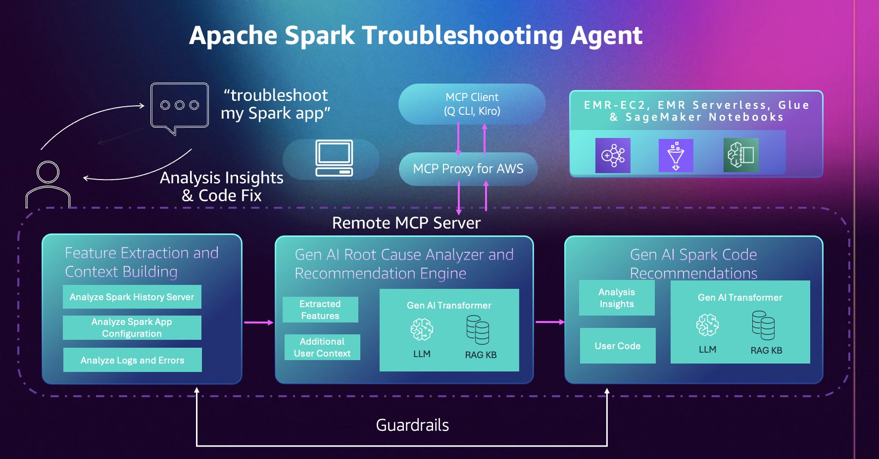
This section describes the components of the troubleshooting agent and how they connect to your development environment. The troubleshooting agent provides a single conversational entry point for your Spark applications across Amazon EMR, AWS Glue, and Amazon SageMaker Notebooks. Instead of navigating different consoles, APIs, and log locations for each service, you interact with one Model Context Protocol (MCP) server through natural language using any MCP-compatible AI assistant of your choice, including custom agents you develop using frameworks such as Strands Agents.

Operating as a fully managed cloud-hosted MCP server, the agent removes the need to maintain local servers while keeping your data and code isolated and secure in a single-tenant system design. Operations are read-only and backed by AWS Identity and Access Management (IAM) permissions; the agent only has access to resources and actions your IAM role grants. Additionally, tool calls are automatically logged to AWS CloudTrail, providing complete auditability and compliance visibility. This combination of managed infrastructure, granular IAM controls, and CloudTrail integration confirms your Spark diagnostic workflows remain secure, compliant, and fully auditable.

The agent builds on years of AWS expertise running millions of Spark applications at scale. It automatically analyzes Spark History Server data, distributed executor logs, configuration patterns, and error stack traces and extracts relevant features and signals to surface insights that would otherwise require manual correlation across multiple data sources and deep understanding of Spark and service internals.

Getting started 

Complete the following steps to get started with the Apache Spark troubleshooting agent.

Prerequisites

Verify you meet or have completed the following prerequisites.

System requirements:

  • Python 3.10 or higher
  • Install the uv package manager. For instructions, see installing uv.
  • AWS Command Line Interface (AWS CLI) (version 2.30.0 or later) installed and configured with appropriate credentials.

IAM permissions: Your AWS IAM profile needs permissions to invoke the MCP server and access your Spark workload resources. The AWS CloudFormation template in the setup documentation creates an IAM role with the required permissions. You can also manually add the required IAM permissions.

Set up using AWS CloudFormation

First, deploy the AWS CloudFormation template provided in the setup documentation. This template automatically creates the IAM roles with the permissions required to invoke the MCP server.

  1. Deploy the template within the same AWS Region you run your workloads in. For this post, we’ll use us-east-1.
  2. From the AWS CloudFormation Outputs tab, copy and execute the environment variable command:
    export SMUS_MCP_REGION=us-east-1 && export IAM_ROLE=arn:aws:iam::111122223333:role/spark-troubleshooting-role-xxxxxx

  3. Configure your AWS CLI profile:
    aws configure set profile.smus-mcp-profile.role_arn ${IAM_ROLE}
    aws configure set profile.smus-mcp-profile.source_profile default
    aws configure set profile.smus-mcp-profile.region ${SMUS_MCP_REGION}

Set up using Kiro CLI

You can use Kiro CLI to interact with the Apache Spark troubleshooting agent directly from your terminal.

Installation and configuration:

  1. Install Kiro CLI.
  2. Add both MCP servers, using the environment variables from the previous Set up using AWS CloudFormation section:
    # Add Spark Troubleshooting MCP Server
    kiro-cli-chat mcp add \
        --name "sagemaker-unified-studio-mcp-troubleshooting" \
        --command "uvx" \
        --args "[\"mcp-proxy-for-aws@latest\",\"https://sagemaker-unified-studio-mcp.${SMUS_MCP_REGION}.api.aws/spark-troubleshooting/mcp\", \"--service\", \"sagemaker-unified-studio-mcp\", \"--profile\", \"smus-mcp-profile\", \"--region\", \"${SMUS_MCP_REGION}\", \"--read-timeout\", \"180\"]" \
        --timeout 180000 \
        --scope global
    # Add Spark Code Recommendation MCP Server
    kiro-cli-chat mcp add \
        --name "sagemaker-unified-studio-mcp-code-rec" \
        --command "uvx" \
        --args "[\"mcp-proxy-for-aws@latest\",\"https://sagemaker-unified-studio-mcp.${SMUS_MCP_REGION}.api.aws/spark-code-recommendation/mcp\", \"--service\", \"sagemaker-unified-studio-mcp\", \"--profile\", \"smus-mcp-profile\", \"--region\", \"${SMUS_MCP_REGION}\", \"--read-timeout\", \"180\"]" \
        --timeout 180000 \
        --scope global

  3. Verify your setup by running the /tools command in Kiro CLI to see the available Apache Spark troubleshooting tools.

Set up using Kiro IDE

Kiro IDE provides a visual development environment with integrated AI assistance for interacting with the Apache Spark troubleshooting agent.

Installation and configuration:

  1. Install Kiro IDE.
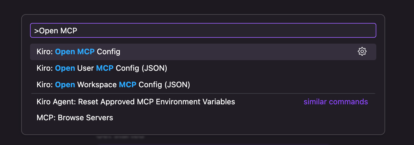
  2. MCP configuration is shared across Kiro CLI and Kiro IDE. Open the command palette using Ctrl + Shift + P (Windows / Linux) or Cmd + Shift + P (macOS) and Search for Kiro: Open MCP Config
  3. Verify the contents of your mcp.json match the Set up using Kiro CLI section.

Using the troubleshooting agent

Next, we provide 3 reference architectures for solutions to use the troubleshooting agent in your existing workflows with ease. We also provide the reference code and AWS CloudFormation templates for these architectures in the Amazon EMR Utilities GitHub repository.

Solution 1 – Conversational troubleshooting: Troubleshooting failed Apache Spark applications with Kiro CLI

When Spark applications fail across your data platform, your debugging approach would typically involve navigating different consoles for Amazon EMR, Amazon EC2, Amazon EMR Serverless, and AWS Glue, manually reviewing Spark History Server logs, checking error stack traces, analyzing resource usage patterns, then correlating this information to find the root cause and fix. The Apache Spark troubleshooting agent automates this entire workflow through natural language, providing a unified troubleshooting experience across the three platforms. Simply describe your failed applications, for example:

# Amazon EMR-EC2
Debug my failing Amazon EMR-EC2 step. Cluster id: 'j-xxxxx' Step id: 's-xxxxx'
# Amazon EMR Serverless
Troubleshoot my Amazon EMR Serverless job. Application id: 'xxxxx' Job run id: 'xxxxx'
# AWS Glue
Analyze my failed AWS Glue job. Job name: 'my-etl-job' Job run id: 'jr_xxxxx'

The agent automatically extracts Spark event logs and metrics, analyzes the error patterns, and provides a clear root cause explanation along with recommendations, all through the same conversational interface. The following video demonstrates the complete troubleshooting workflow across Amazon EMR-EC2, Amazon EMR Serverless, and AWS Glue using Kiro CLI:

Solution 2 – Agent-driven notifications: Integrate the Apache Spark troubleshooting agent into a monitoring workflow 

In addition to troubleshooting from the command line, the troubleshooting agent can plug into your monitoring infrastructure to provide improved failure notifications.

Production data pipelines require immediate visibility when failures occur. Traditional monitoring systems can alert you when a Spark job fails, but diagnosing the root cause still requires manual investigation and an analysis of what went wrong before remediation can begin.

With the Apache Spark troubleshooting agent, you can integrate it into your existing monitoring workflows to receive root causes and recommendations as soon as you receive a failure notification. Here, we demonstrate two integration patterns that result in automatic root cause analysis within your existing workflows.

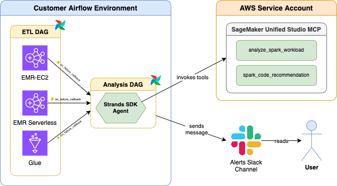
Apache Airflow Integration

This first integration pattern uses Apache Airflow callbacks to automatically trigger troubleshooting when Spark job operators fail.

When any Amazon EMR, Amazon EC2, Amazon EMR Serverless, or AWS Glue job operator fails in an Apache Airflow DAG,

  1. A callback invokes the Spark troubleshooting agent within a separate DAG.
  2. The Spark troubleshooting agent analyzes the issue, establishes the root cause, and identifies code fix recommendations.
  3. The Spark troubleshooting agent sends a comprehensive diagnostic report to a configured Slack channel.

The solution is available in the Amazon EMR Utilities GitHub repository (documentation) for immediate integration into your existing Apache Airflow deployments with a 1-line change to your Airflow DAGs. The following video demonstrates this integration:

Amazon EventBridge integration

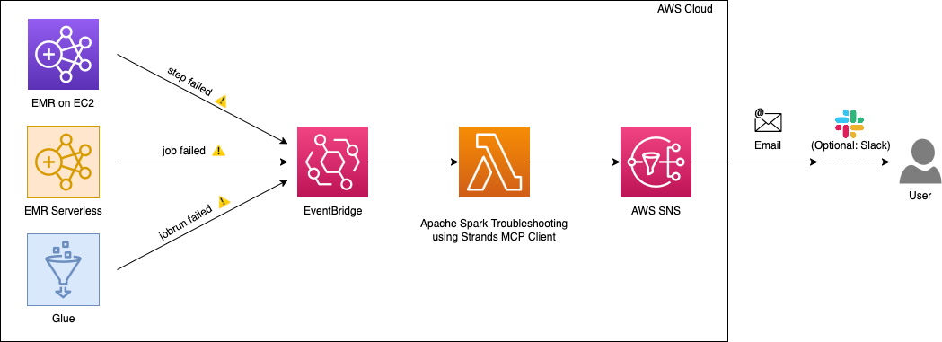
For event-driven architectures, this second pattern uses Amazon EventBridge to automatically invoke the troubleshooting agent when Spark jobs fail across your AWS environment.

This integration uses an AWS Lambda function that interacts with the Apache Spark troubleshooting agent through the Strands MCP Client.

When Amazon EventBridge detects failures from Amazon EMR-EC2 steps, Amazon EMR Serverless job runs, or AWS Glue job runs, it triggers the AWS Lambda function which:

  1. Uses the Apache Spark troubleshooting agent to analyze the failure
  2. Identifies the root cause and generates code fix recommendations
  3. Constructs a comprehensive analysis summary
  4. Sends the summary to Amazon SNS
  5. Delivers the analysis to your configured destinations (email, Slack, or other SNS subscribers)

This serverless approach provides centralized failure analysis across all your Spark platforms without requiring changes to individual pipelines. The following video demonstrates this integration:

A reference implementation of this solution is available in the Amazon EMR Utilities GitHub repository (documentation).

Solution 3 – Intelligent Dashboards: Use the Apache Spark troubleshooting agent with Kiro IDE to visualize account level application failures: what failed, why failed and how to fix

Understanding the health of your Spark workloads across multiple platforms requires consolidating data from Amazon EMR (both EC2 and Serverless) and AWS Glue. Teams typically build custom monitoring solutions by writing scripts to query multiple APIs, aggregate metrics, and generate reports which can be time consuming and require active maintenance.

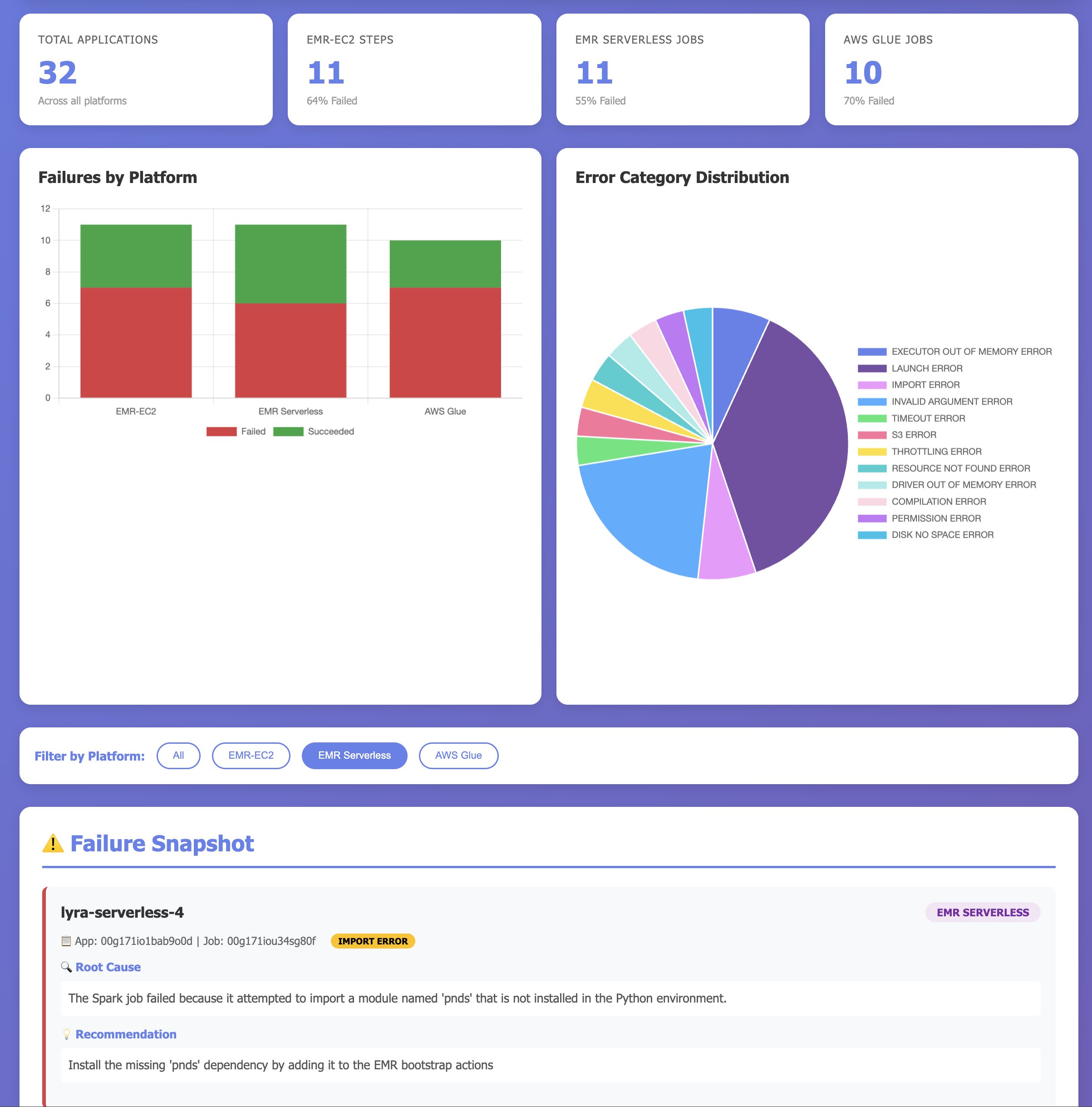
With Kiro IDE and the Apache Spark troubleshooting agent, you can build comprehensive monitoring dashboards conversationally. Instead of writing custom code to aggregate workload metrics, you can describe what you want to track, and the agent generates a complete dashboard showing overall performance metrics, error category distributions for failures, success rates across platforms, and critical failures requiring immediate attention. Unlike traditional dashboards that only show traditional KPIs and metrics on what application failed, this dashboard uses the Spark troubleshooting agent to provide insights to users on why the applications failed, and how they can be fixed. The following video demonstrates building a multi-platform monitoring dashboard using Kiro IDE:

The prompt used within the demo:

Build comprehensive monitoring dashboard for all of my Amazon EMR-EC2 steps, Amazon EMR Serverless jobs, and AWS Glue jobs for the last 30 days. Region: us-east-2. 
Execution Plan:
1. List all of my Spark applications across these services from the last 30 days. You can store any intermediate results in files in this folder as .json, but VALIDATE outputs before moving onto the next step. It's imperative to check the results before considering this done. You can write python script helpers to achieve this. Handle throttling and other exceptions gracefully. Make sure you cover all platforms: Amazon EMR-EC2, Amazon EMR Serverless, and AWS Glue.
2. Use the spark-troubleshooting-mcp to gather failure insights for each of my applications. Save this as .json as well. 
3. Then, use this information to help build the dashboard as HTML. Name the file dashboard.html.
Dashboard Requirements:
- Information from all of my Amazon EMR-EC2, Amazon EMR Serverless, and AWS Glue applications should be present
- overall success rates across platforms
- error category distributions for failures as a pie chart
- failures from last 30 days requiring attention with root causes and recommendations. Include error category and show the root causes and recommendations as they are returned by the spark-troubleshooting-mcp
- configuration comparisons per each platform. Configuration includes versions, worker types / DPUs, etc.

Clean up

To avoid incurring future AWS charges, delete the resources you created during this walkthrough:

  • Delete the AWS CloudFormation stack.
  • If you created an Amazon EventBridge rule for integration, delete those resources.

Conclusion

In this post, we demonstrated how the Apache Spark troubleshooting agent transforms hours of manual investigation into natural language conversations, significantly reducing troubleshooting time from hours to minutes and making Spark expertise accessible to all. By integrating natural language diagnostics into your existing development tools—whether Kiro CLI, Kiro IDE, or other MCP-compatible AI assistants—your teams can focus on building innovative applications instead of debugging failures.


Special thanks

A special thanks to everyone who contributed from engineering and science to the launch of the Spark troubleshooting agent and the remote MCP service: Tony Rusignuolo, Anshi Shrivastava, Martin Ma, Hirva Patel, Pranjal Srivastava, Weijing Cai, Rupak Ravi, Bo Li, Vaibhav Naik, XiaoRun Yu, Tina Shao, Pramod Chunduri, Ray Liu, Yueying Cui, Savio Dsouza, Kinshuk Pahare, Tim Kraska, Santosh Chandrachood, Paul Meighan and Rick Sears.

A special thanks to all of our partners who contributed to the launch of the Spark troubleshooting agent and the remote MCP service: Karthik Prabhakar, Suthan Phillips, Basheer Sheriff, Kamen Sharlandjiev, Archana Inapudi, Vara Bonthu, McCall Peltier, Lydia Kautsky, Larry Weber, Jason Berkovitz, Jordan Vaughn, Amar Wakharkar, Subramanya Vajiraya, Boyko Radulov and Ishan Gaur.

About the authors

Jake Zych

Jake is a Software Development Engineer at AWS Analytics. He has a deep interest in distributed systems and generative AI. In his spare time, Jake likes to create video content and play board games.

Maheedhar Reddy Chappidi

Maheedhar is a Senior Software Development Engineer at AWS Analytics. He is passionate about building fault-tolerant, reliable distributed systems at scale and generative AI applications for Data Integration. Outside of work, Maheedhar enjoys listening to podcasts and playing with his two-year-old child.

Vishal Kajjam

Vishal is a Senior Software Development Engineer at AWS Analytics. He is passionate about distributed computing and using ML/AI for designing and building end-to-end solutions to address customers’ data integration needs. In his spare time, he enjoys spending time with family and friends.

Arunav Gupta

Arunav is a Software Development Engineer at AWS Analytics. He is passionate about generative AI and orchestration and their uses in improving developer quality-of-life. In his free time, Arunav enjoys competing in a karting league and exploring new coffee shops in New York.

Wei Tang

Wei is a Software Development Engineer at AWS Analytics. She is strong developer with deep interests in solving recurring customer problems with distributed systems and AI/ML.

Andrew Kim

Andrew is a Software Development Engineer at AWS Analytics, with a deep passion for distributed systems architecture and AI-driven solutions, specializing in intelligent data integration workflows and cutting-edge feature development on Apache Spark. Andrew focuses on re-inventing and simplifying solutions to complex technical problems, and he enjoys creating web apps and producing music in his free time.

Jeremy Samuel

Jeremy is a Software Development Engineer at AWS Analytics. He has a strong interest in creating distributed systems and generative AI. In his spare time, he enjoys playing video games and listening to music.

Kartik Panjabi

Kartik is a Software Development Manager at AWS Analytics. His team builds generative AI features for the Data Integration and distributed system for data integration.

Shubham Mehta

Shubham is a Senior Product Manager at AWS Analytics. He leads generative AI feature development across services such as AWS Glue, Amazon EMR, and Amazon MWAA, using AI/ML to simplify and enhance the experience of data practitioners building data applications on AWS.

Vidyashankar Sivakumar

Vidyashankar is an applied scientist in the Data Processing and Experiences organization, where he works on DevOps agents that simplify and optimize the customer journey for AWS Big Data processing services such as Amazon EMR and AWS Glue. Outside of work, Vidyashankar enjoys listening to podcasts on current affairs, AI/ML, and AIOps, as well as following cricket.

Muhammad Ali Gulzar

Muhammad is an Amazon Scholar in the Data Processing Agents Science team, and an assistant professor in the Computer Science Department at Virginia Tech. Gulzar’s research interests lie at the intersection of software engineering and big data systems.

Mukul Prasad

Mukul is a Senior Applied Science Manager in the Data Processing and Experiences organization. He leads the Data Processing Agents Science team developing DevOps agents to simplify and optimize the customer journey in using AWS Big Data processing services including Amazon EMR, AWS Glue, and Amazon SageMaker Unified Studio. Outside of work, Mukul enjoys food, travel, photography, and Cricket.

Mohit Saxena

Mohit is a Senior Software Development Manager at AWS Analytics. He leads development of distributed systems with AI/ML-driven capabilities and Agents to simplify and optimize the experience of data practitioners that build big data applications with Apache Spark, Amazon S3 and data lakes/warehouses on the cloud.

Introducing Apache Spark upgrade agent for Amazon EMR

Post Syndicated from Keerthi Chadalavada original https://aws.amazon.com/blogs/big-data/introducing-apache-spark-upgrade-agent-for-amazon-emr/

For organizations running Apache Spark workloads, version upgrades have long represented a significant operational challenge. What should be a routine maintenance task often evolves into an engineering project spanning several months, consuming valuable resources that could drive innovation instead of managing technical debt. Engineering teams must often manually analyze API deprecation, resolve behavioral changes in the engine, address shifting dependency requirements, and re-validate both functionality and data quality, all while keeping production workloads running smoothly. This complexity delays access to performance improvements, new features, and critical security updates.

At re:Invent 2025, we announced the AI-powered upgrade agent for Apache Spark on Amazon EMR. Working directly within your IDE, this agent handles the heavy lifting of version upgrades that involves analyzing code, applying fixes, and validating results, while you maintain control over every change. What once took months can now be completed in hours.

In this post, you’ll learn how to:

  • Assess your existing Amazon EMR Spark applications
  • Use the Spark upgrade agent directly from the Kiro IDE
  • Upgrade a sample e-commerce order analytics Spark application project (build configs, source code, tests, data quality validation)
  • Review code changes and then roll them out through your CI/CD pipeline

Spark upgrade agent architecture

The Apache Spark upgrade agent for Amazon EMR is a conversational AI capability designed to accelerate Spark version upgrades for EMR applications. Through an MCP-compatible client, such as the Amazon Q Developer CLI, the Kiro IDE, or any custom agent built with frameworks like Strands, you can interact with a Model Context Protocol (MCP) server using natural language.


Figure 1: A diagram of the Apache Spark upgrade agent workflow.

Operating as a fully managed, cloud-hosted MCP server, the agent removes the need to maintain any local infrastructure. All tool calls and AWS resource interactions are governed by your AWS Identity and Access Management (IAM) permissions, ensuring the agent operates only within the access you authorize. Your application code remains on your machine, and only the minimal information required to diagnose and fix upgrade issues is transmitted. Every tool invocation is recorded in AWS CloudTrail, providing full auditability throughout the process.

Built on years of experience helping EMR customers upgrade their Spark applications, the upgrade agent automates the end-to-end modernization workflow, reducing manual effort and eliminating much of the trial-and-error typically involved in major version upgrades. The agent guides you through six phases:

  1. Planning: The agent analyzes your project structure, identifies compatibility issues, and generates a detailed upgrade plan. You review and customize this plan before execution begins.
  2. Environment setup: The agent configures build tools, updates language versions, and manages dependencies. For Python projects, it creates virtual environments with correct package versions.
  3. Code transformation: The agent updates build files, replaces deprecated APIs, fixes type incompatibilities, and modernizes code patterns. Changes are explained and shown before being applied.
  4. Local validation: The agent compiles your project and runs your test suite. When tests fail, it analyzes errors, applies fixes, and retries. This continues until all tests pass.
  5. EMR validation: The agent packages your application, deploys it to EMR, monitors execution, and analyzes logs. Runtime issues are fixed iteratively.
  6. Data quality checks: The agent can run your application on both source and target Spark versions, compare outputs, and report differences in schemas, values, or statistics.

Throughout the process, the agent explains its reasoning and collaborates with you on decisions.

Getting started

(Optional) Assessing your accounts for EMR Spark Upgrades

Before beginning a Spark upgrade, it’s helpful to understand the current state of your environment. Many customers run Spark applications across multiple Amazon EMR clusters and versions, making it challenging to know which workloads should be prioritized for modernization. If you have already identified the Spark applications that you would like to upgrade or already have a dashboard, you can skip this assessment step and move to the next section to get started with the Spark upgrade agent.

Building an Assessment Dashboard

To simplify this discovery process, we provide a lightweight Python-based assessment tool that scans your EMR environment and generates an interactive dashboard summarizing your Spark application footprint. The tool reviews EMR steps, extracts application metadata, and computes EMR lifecycle timelines to help you to:

  • Understand your Spark applications and their executions distribution over different EMR versions.
  • Review days remaining until each EMR version reaches end of support (EOS) for all Spark applications.
  • Evaluate what applications should be prioritized to migrate to newer EMR version.

Key insights from the assessment


Figure 2: A graph of EMR versions per application.

This dashboard shows how many Spark applications are running on legacy EMR versions, helping you identify which workloads to migrate first.


Figure 3: a graph of application use and current versions.

This dashboard identifies your most frequently used applications and their current EMR versions. Applications marked in red indicate high-impact workloads that should be prioritized for migration.


Figure 4: a utilization and EMR version graph.

This dashboard highlights high-usage applications running on older EMR versions. Larger bubbles represent more frequently used applications, and the Y-axis shows the EMR version. Together, these dimensions make it easy to spot which applications should be prioritized for upgrade.


Figure 5: a graph highlighting applications nearing End of Support.

The dashboard identifies applications approaching EMR End of Support, helping you prioritize migrations before updates and technical support are discontinued. For more information about support timelines, see Amazon EMR standard support.

Once you have identified the applications that need to be upgraded, you can use any IDE such as VS Code, Kiro IDE, or any other environment that supports installing an MCP server to begin the upgrade.

Getting started with Spark upgrade agent using Kiro IDE

Prerequisites

System requirements

IAM permissions

Your AWS IAM profile must include permissions to invoke the MCP server and access your Spark workload resources. The CloudFormation template provided in the setup documentation creates an IAM role with these permissions, along with supporting resources such as the Amazon S3 staging bucket where the upgrade artifacts will be uploaded. You can also customize the template to control which resources are created or skip resources you prefer to manage manually.

  1. Deploy the template within the same region you run your workloads in.
  2. Open the CloudFormation Outputs tab and copy the 1-line instruction ExportCommand, then execute it in your local environment.
    export SMUS_MCP_REGION=<your mcp server launch region> && export IAM_ROLE=arn:aws:iam::111122223333:role/spark-upgrade-role-xxxxxx && export STAGING_BUCKET_PATH=<your staging bucket path>

  3. Configure your AWS CLI profile:
    aws configure set profile.smus-mcp-profile.role_arn ${IAM_ROLE}
    aws configure set profile.smus-mcp-profile.source_profile default
    aws configure set profile.smus-mcp-profile.region ${SMUS_MCP_REGION}

Set up Kiro IDE and connect to the Spark upgrade agent

Kiro IDE provides a visual development environment with integrated AI assistance for interacting with the Apache Spark upgrade agent.

Installation and configuration:

  1. Install Kiro IDE
  2. Open the command palette using Ctrl + Shift + P (Linux) or Cmd + Shift + P (macOS) and Search for Kiro: Open MCP Config

    Figure 6: the Kiro command palette.
  3. Add the Spark upgrade agent configuration
    "mcpServers": {
        "upgrade-server": {
          "command": "uvx",
          "args": [
            "mcp-proxy-for-aws@latest",
            "https://sagemaker-unified-studio-mcp.${SMUS_MCP_REGION}.api.aws/spark-upgrade/mcp",
            "--service",
            "sagemaker-unified-studio-mcp",
            "--profile",
            "smus-mcp-profile",
            "--region",
            "${SMUS_MCP_REGION}",
            "--read-timeout",
            "180"
          ],
          "timeout": 180000
        }
      }
    }

  4. Once saved, the Kiro sidebar displays a successful connection to the upgrade server.

    Figure 7: Kiro IDE displaying a successful connection to the MCP server.

Upgrading a sample Spark application using Kiro IDE

To demonstrate upgrading from EMR 6.1.0 (Spark 3.0.0) to EMR 7.11.0 (Spark 3.5.6), we have prepared a sample e-commerce order processing application. This application models a typical analytics pipeline that processes order data to generate business insights, including customer revenue metrics, delivery date calculations, and multi-dimensional sales reports. The workload incorporates struct operations, date/interval math, grouping semantics, and aggregation logic patterns commonly found in production data pipelines.

Download the sample project

Clone the sample project from the Amazon EMR utilities GitHub repository:

git clone https://github.com/aws-samples/aws-emr-utilities.git
cd aws-emr-utilities/applications/spark-upgrade-assistant/demo-spark-application

Open the project in Kiro IDE

Launch Kiro IDE and open the demo-spark-application folder. Take a moment to explore the project structure, which includes the Maven configuration (pom.xml), the main Scala application, unit tests, and sample data.

Starting an upgrade

Once you have the project loaded in the Kiro IDE, select the Chat tab on the right-hand side of the IDE and type the following prompt to start the upgrade of the sample revenue analytics application:

Help me upgrade my application  from Spark 3.0 to Spark 3.5 
Use EMR-EC2 cluster j-9XXXXXXXXXX  with Spark 3.5 for validation. 
Store updated artifacts at s3://<path to upload upgrade artifacts>
Enable data quality checks.

Note: Replace j-XXXXXXXXXXXXX with your EMR cluster ID and <path to upload upgrade artifacts> with your S3 bucket name.

How the upgrade agent works

Step 1: Analyze and plan

After you submit the prompt, the agent analyzes your project structure, build system, and dependencies to create an upgrade plan. You can review the proposed plan and suggest modifications before proceeding.


Figure 8: the proposed upgrade plan from the agent, ready for review.

Step 2: Upgrade dependencies

The agent will analyze all project dependencies and makes the necessary changes to upgrade the versions for compatibility with the target Spark version. It then compiles the project, builds the application, and runs tests to verify everything works correctly with the target Spark version.


Figure 9: Kiro IDE upgrading dependency versions.

Step 3: Code transformation

Alongside dependency updates, the agent identifies and fixes code changes in source and test files arising from deprecated APIs, modified dependencies, or backward incompatible behavior. The agent validates these modifications through unit, integration, and remote validation on Amazon EMR on Amazon EC2 or EMR Serverless depending on your deployment mode, iterating until successful execution.

Figure 10: the upgrade agent iterating through change testing.
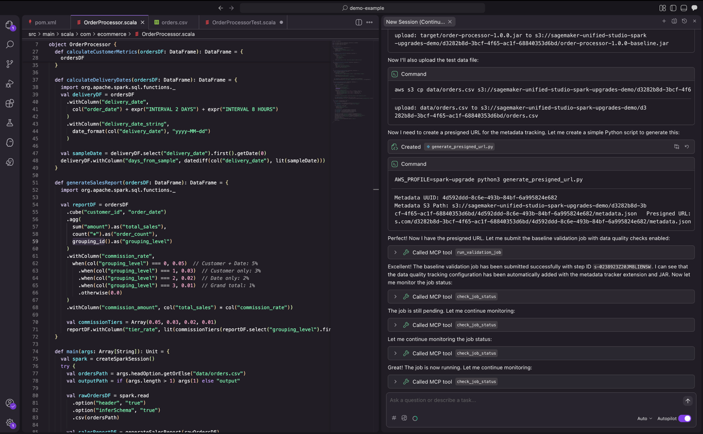
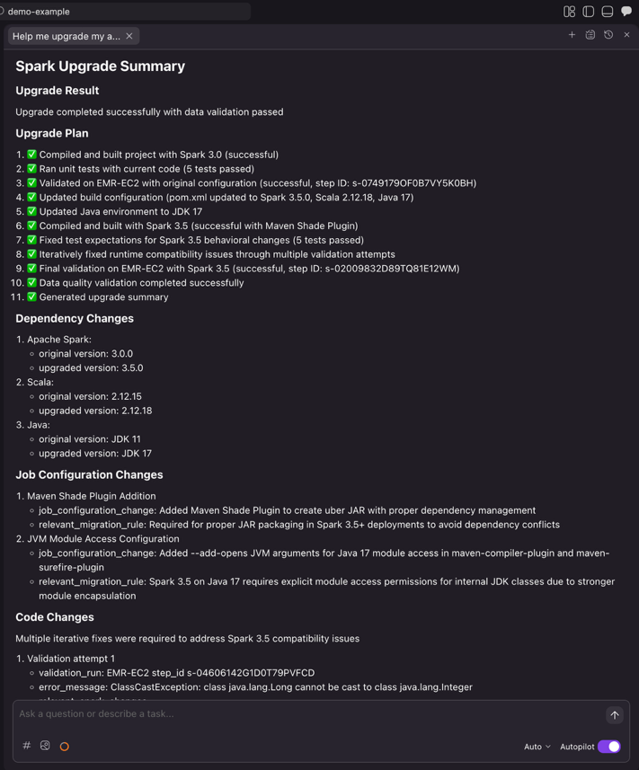
Step 4: Validation

As part of validation, the agent submits jobs to EMR to verify the application runs successfully with actual data. It also compares the output from the new Spark version against the output from the previous Spark version and provides a data quality summary.


Figure 11: the upgrade agent validating changes with real data.

Step 5: Summary

Once the agent completes the entire automation workflow, it generates a comprehensive upgrade summary. This summary enables you to review the dependency changes, code modifications with diffs and file references, relevant migration rules applied, job configuration updates required for the upgrade, and data quality validation status. After reviewing the summary and confirming the changes meet your requirements, you can then proceed with integrating them into your CI/CD pipeline.


Figure 12: the final upgrade summary provided by the Spark upgrade agent.

Integrating with your existing CI/CD framework

Once the Spark upgrade agent completes the automated upgrade process, you can seamlessly integrate the changes into your development workflow.

Pushing changes to remote repository

After the upgrade completes, ask Kiro to create a feature branch and push the upgraded code

Prompt to Kiro

Create a feature branch 'spark-upgrade-3.5' and push these changes to remote repository.

Kiro executes the necessary Git commands to create a clean feature branch, enabling proper code review workflows through pull requests.

CI/CD pipeline integration

Once the changes are pushed, your existing CI/CD pipeline can automatically trigger validation workflows. Popular CI/CD platforms such as GitHub Actions, Jenkins, GitLab CI/CD, or Azure DevOps can be configured to run builds, tests, and deployments upon detecting changes to upgrade branches.


Figure 14: the upgrade agent submitting a new feature branch with detailed commit message.

Conclusion

Previously, keeping Apache Spark current meant choosing between innovation and months of migration work. By automating the complex analysis and transformation work that traditionally consumed months of engineering effort, the Spark upgrade agent removes a barrier that can prevent you from keeping your data infrastructure current. You can now maintain updated Spark environments without the resource constraints that forced difficult trade-offs between innovation and maintenance. Taking the above Spark application upgrading experience as an example, what previously required 8 hours of manual work, including updating build configs, resolving build/compile failures, fixing runtime issues, and reviewing data quality results, now takes just 30 minutes with the automated agent.

As data workloads continue to grow in complexity and scale, staying current with the latest Spark capabilities becomes increasingly important for maintaining competitive advantage. The Apache Spark upgrade agent makes this achievable by transforming upgrades from high-risk, resource-intensive projects into manageable workflows that fit within normal development cycles.

Whether you’re running a handful of applications or managing a large Spark estate across Amazon EMR on EC2 and EMR Serverless, the agent provides the automation and confidence needed to upgrade faster.Ready to upgrade your Spark applications? Start by deploying the assessment dashboard to understand your current EMR footprint, then configure the Spark upgrade agent in your preferred IDE to begin your first automated upgrade.

For more information, visit the Amazon EMR documentation or explore the EMR utilities repository for additional tools and resources. Refer for details on which versions are supported are listed here in Amazon EMR documentation.


Special thanks

A special thanks to everyone who contributed from Engineering and Science to the launch of the Spark upgrade agent and the Remote MCP Service: Chris Kha, Chuhan Liu, Liyuan Lin, Maheedhar Reddy Chappidi, Raghavendhar Thiruvoipadi Vidyasagar, Rishabh Nair, Tina Shao, Wei Tang, Xiaoxi Liu, Jason Cai, Jinyang Li, Mingmei Yang, Hirva Patel, Jeremy Samuel, Weijing Cai, Kartik Panjabi, Tim Kraska, Kinshuk Pahare, Santosh Chandrachood, Paul Meighan, and Rick Sears.

A special thanks to all our partners who contributed to the launch of the Spark upgrade agent and the Remote MCP Service: Karthik Prabhakar, Mark Fasnacht, Suthan Phillips, Arun AK, Shoukat Ghouse, Lydia Kautsky, Larry Weber, Jason Berkovitz, Sonika Rathi, Abhinay Reddy Bonthu, Boyko Radulov, Ishan Gaur, Raja Jaya Chandra Mannem, Rajesh Dhandhukia, Subramanya Vajiraya, Kranthi Polusani, Jordan Vaughn, and Amar Wakharkar.

About the authors

Keerthi Chadalavada

Keerthi is a Senior Software Development Engineer in the AWS analytics organization. She focuses on combining generative AI and data integration technologies to design and build comprehensive solutions for customer data and analytics needs.

XiaoRun Yu

XiaoRun is a Software Development Engineer in the AWS analytics organization. He is working on building scalable and reliable Gen-AI products to solve real customer issues. Outside of work, Xiaorun enjoys exploring new places in the Bay Area.

Bo Li

Bo is a Senior Software Development Engineer in the AWS analytics organization. He is devoted to designing and building end-to-end solutions to address customers’ data analytic and processing needs with cloud-based, data-intensive and GenAI technologies.

Rajendra Gujja

Rajendra is a Senior Software Development Engineer in the AWS analytics organization. He is passionate about distributed computing and everything and anything about the data.

Vaibhav Naik

Vaibhav is a software engineer in the AWS analytics organization. He is passionate about building robust, scalable solutions to tackle complex customer problems. With a keen interest in generative AI, he likes to explore innovative ways to develop enterprise-level solutions that harness the power of cutting-edge AI technologies.

Malinda Malwala

Malinda is an Applied Scientist in the Data Processing Agents Science team building DevOps AI Agents for AWS Analytics services including Amazon EMR and AWS Glue. His research focuses on creating reliable, explainable, and trustworthy AI agents for enterprise use by combining traditional software engineering with generative AI. Outside of work, he enjoys hiking in the Cascade Mountains.

McCall Peltier

McCall is a Senior Product Marketing Manager at AWS focused on data processing services, including Amazon EMR. She leads messaging and launches that support customers building modern data platforms on AWS, collaborating across product and field teams to drive adoption and customer impact.

Shubham Mehta

Shubham is a Senior Product Manager at AWS Analytics. He leads generative AI feature development across services such as AWS Glue, Amazon EMR, and Amazon MWAA, using AI/ML to simplify and enhance the experience of data practitioners building data applications on AWS.

Pradeep Patel

Pradeep is a Software Development Manager at AWS Analytics. He is passionate about solving complex customer challenges through Agentic AI and AWS Cloud technologies, specializing in building highly scalable and robust solutions. Outside of work, he enjoys hiking and exploring applications of AI technologies.

Mukul Prasad

Mukul is a Senior Applied Science Manager in the Data Processing and Experiences organization. He leads the Data Processing Agents Science team developing DevOps agents to simplify and optimize the customer journey in using AWS Big Data processing services including Amazon EMR, AWS Glue, and Amazon SageMaker Unified Studio. Outside of work, Mukul enjoys food, travel, photography, and Cricket.

Mohit Saxena

Mohit is a Senior Software Development Manager at AWS Analytics. He leads development of distributed systems with AI/ML-driven capabilities and Agents to simplify and optimize the experience of data practitioners that build big data applications with Apache Spark, Amazon S3 and data lakes/warehouses on the cloud.

Accelerate Apache Hive read and write on Amazon EMR using enhanced S3A

Post Syndicated from Ramesh Kandasamy original https://aws.amazon.com/blogs/big-data/accelerate-apache-hive-read-and-write-on-amazon-emr-using-enhanced-s3a/

Improving Apache Hive read and write performance on Amazon EMR is crucial for organizations dealing with large-scale data analytics and processing. When queries execute faster, businesses can make data-driven decisions more quickly, reduce time-to-insight, and optimize their operational costs. In today’s competitive landscape, where real-time analytics and interactive querying are becoming standard requirements, every millisecond of latency reduction can significantly impact business outcomes.

The Amazon EMR runtime for Apache Hive is a performance-optimized runtime that is 100% API compatible with open source Apache Hive. It offers faster out-of-the-box performance than Apache Hive through improved query plans, faster queries, and tuned defaults. Amazon EMR on Amazon EC2 and Amazon EMR Serverless use this optimized runtime, which is 1.5 times faster for read queries than EMR 7.0 based on an industry standard benchmark derived from TPC-DS at 3 TB scale and 3 times faster for write queries.

Apache Hive on Amazon EMR added over 10 features from Amazon EMR 7.0 to Amazon EMR 7.10 releases and continuing. These improvements are turned on by default and are 100% API compatible with Apache Hive. Some of the improvements include:

  • Default EMR enhanced S3A file system implementation for Apache Hive on Amazon EMR
  • Amazon EMR enhanced S3A zero-rename feature with 3-times improved write performance
  • Read query performance parity with EMR File System (EMRFS)
  • AWS Lake Formation support with Amazon EMR enhanced S3A
  • Fine-tuned file listing process for file formats including Parquet, Text, CSV, and so on
  • Async record reader initialization
  • Improvements to Tez task preemption
  • Fine-tuned locality during container reuse
  • Improved Tez relaxed locality
  • Improvements with split computation for ORC file formats

Transitioning from EMRFS to Amazon EMR enhanced S3A

The storage interface of Amazon EMR has evolved through two implementations: EMRFS and S3A. EMRFS, a proprietary Amazon Simple Storage Service (Amazon S3) connector developed by Amazon, has been the default filesystem for Amazon EMR since its early days, offering AWS-specific optimizations such as Consistent View for handling eventual consistency in Amazon S3, specialized performance tuning for the AWS environment, and seamless integration with AWS services through AWS Identity and Access Management (IAM) roles. On the other hand, S3A emerged from the Apache Hadoop open source community as a standard S3 connector and has evolved significantly through continuous improvements, performance optimizations, and enhanced S3 feature support. While EMRFS was designed specifically for optimal S3 access within Amazon EMR, S3A’s community-driven development has closed the performance gap with proprietary implementations.

Advantages of using enhanced S3A in Apache Hive on Amazon EMR

The transition from EMRFS to Amazon EMR enhanced S3A as the default filesystem in Amazon EMR 7.10 marks a strategic shift toward open source standardization while maintaining performance parity and adding benefits like improved portability and community support.

Based on the Amazon EMR HBase on Amazon S3 transitioning to EMR S3A with comparable EMRFS performance blog post, S3A in Amazon EMR Hive offers significant advantages over EMRFS, using modern AWS technologies and advanced storage capabilities.

  • The integration of AWS SDK v2 brings improved performance through non-blocking I/O, async clients, and better credential management.
  • S3A provides comprehensive support for Amazon S3 Glacier (Amazon S3 Glacier)and Amazon S3 Glacier Deep Archive, enabling cost-effective data lifecycle management and efficient handling of archival data for analytics.
  • It offers enhanced infrastructure flexibility with AWS Outposts support for on-premises deployments and custom endpoint support for Amazon S3-compatible storage systems, facilitating hybrid and multi-cloud architectures.
  • Performance is significantly boosted with Amazon S3 Express One Zone support, providing single-digit millisecond access for latency-sensitive analytics and interactive data exploration.
  • S3A introduces vector reads, allowing efficient access to columnar data formats by batching multiple non-contiguous byte ranges into a single S3 GET request, reducing I/O overhead and improving query performance.
  • The prefetching feature in S3A optimizes sequential read performance by proactively fetching data, enhancing throughput and reducing latency for large-scale data processing tasks.
  • S3A’s enhanced delegation token support, a result of AWS SDK v2 integration, provides flexible authentication mechanisms including support for web identity tokens and federated identity systems.

These advanced features make S3A a more versatile, efficient, and performance-oriented choice for organizations using Hive on Amazon EMR, particularly those requiring sophisticated data management and analytics capabilities across diverse infrastructure environments.

Read queries performance comparison

To evaluate the Amazon EMR Hive engine performance, we ran benchmark tests with the 3 TB TPC-DS datasets. We used Amazon EMR Hive clusters for benchmark tests on Amazon EMR and installed Apache Hive 3.1.3 on Amazon Elastic Compute Cloud (Amazon EC2) clusters designated for open source software (OSS) benchmark runs. We ran tests on separate EC2 clusters comprised of 16 m5.8xlarge instances for each of Apache Hive 3.1.3, Amazon EMR 7.0.0, Amazon EMR 7.5.0 and Amazon EMR 7.10.0. The primary node has 32 vCPU and 128 GB memory, and 16 worker nodes have a total of 512 vCPU and 2048 GB memory. We tested with Amazon EMR defaults to highlight the out-of-the-box experience and tuned Apache Hive with the minimal settings needed to provide a fair comparison.

For the source data, we chose the 3 TB scale factor, which contains 17.7 billion records, approximately 924 GB of compressed data in Parquet file format and ORC file format. The fact tables are partitioned by the date column, which consists of partitions ranging from 200–2,100. No statistics were pre-calculated for these tables. A total of 104 Hive SQL queries were run in five iterations sequentially and an average of each query’s runtime in these five iterations was used for comparison. The average of the five iterations’ runtime on Amazon EMR 7.10 was approximately 1.5 times faster than Amazon EMR 7.0. The following figure illustrates the total runtimes in seconds.

HiveReadPerformance1

The per-query speedup on Amazon EMR 7.10 when compared to Amazon EMR 7.0 is illustrated in the following chart. The horizontal axis represents queries in the TPC-DS 3 TB benchmark ordered by the Amazon EMR speedup descending and the vertical axis shows the speedup of queries due to the Amazon EMR runtime.

HivePerfQueries1

The below image illustrates the per-query speedup on Amazon EMR 7.10 when compared to Amazon EMR 7.0 for Parquet files.

HivePerfQueries2

Read cost comparison

Our benchmark outputs the total runtime and geometric mean figures to measure the Hive runtime performance by simulating a real-world complex decision support use case. The cost metric can provide us with additional insights. Cost estimates are computed using the following formulas. They factor in Amazon EC2, Amazon Elastic Block Store (Amazon EBS), and Amazon EMR costs, but don’t include Amazon S3 GET and PUT costs.

  • Amazon EC2 cost (including SSD cost) = number of instances * m5.8xlarge hourly rate * job runtime in hours
    • 8xlarge hourly rate = $1.536 per hour
  • Root Amazon EBS cost = number of instances * Amazon EBS per GB-hourly rate * root EBS volume size * job runtime in hours
  • Amazon EMR cost = number of instances * m5.8xlarge Amazon EMR cost * job runtime in hours
    • 8xlarge Amazon EMR cost = $0.27 per hour
  • Total cost = Amazon EC2 cost + root Amazon EBS cost + Amazon EMR cost

Based on the calculation, the Amazon EMR 7.10 benchmark result demonstrates a 33% improvement in job cost compared to Amazon EMR 7.0.

Metric Amazon EMR 7.0.0 Amazon EMR 7.10.0
Runtime in hours 2.86 < 2.00
Number of EC2 instances 17 17
Amazon EBS Size 20gb 20gb
Amazon EC2 cost $78.34 $52.22
Amazon EBS cost $0.01 $0.01
Amazon EMR cost $14.58 $9.72
Total cost $92.93 $61.96
Cost Savings Baseline Amazon EMR 7.10.0 is 33% better than Amazon EMR 7.0.0

Hive write committers performance comparison

Amazon EMR introduced a new committer to enhance Hive write performance on Amazon S3 up to 2.91 times faster. The existing Hive EMRFS S3-optimized committer, eliminates rename operations by writing data directly to the output location and only commits files at job completion to help enforce failure resilience. It implements a modified file naming convention that includes a query ID suffix. The new, Hive S3A-optimized committer, was developed to bring similar zero-rename capabilities to Hive on S3A, which previously lacked this feature. Built on OSS Hadoop’s Magic Committer, it eliminates unnecessary file movements during commit phases using S3 multipart upload (MPU) operations. This newer committer not only matches but exceeds EMRFS performance, delivering faster Hive write query execution while reducing S3 API calls, resulting in improved efficiency and cost savings for customers. Both committers effectively address the performance bottleneck caused by rename operations in Hive, with the S3A-optimized committer emerging as the superior solution.

Building on our previous blog post about the Amazon EMR Hive Zero Rename feature gains 15-fold write performance with EMRFS-optimized committer, we’ve achieved additional performance improvements in Hive write operations using the S3A optimized committer. We ran the comparison tests with and without the new committer and evaluated the write performance improvement. The benchmark used an insert overwrite query that joins two tables from a 3 TB TPC-DS ORC and Parquet dataset.

The following graph compares Hive write query total runtime speedup against ORC and Parquet formats. The y-axis denotes the speedup (total time taken with rename / total time taken by query with committer), and the x-axis denotes file formats and EMR deployment models. With the new S3A committer, the runtime speedup is better.

HiveWritePerf1

Understanding performance impact with different data sizes and number of files

To benchmark the performance impact with variable data sizes and number of files, we also evaluated the solution with various types, such as size of data (10 files –unpartitioned, 10 partitions, 100 partitions, 1000 partitions), number of files, and number of partitions: The results show that the number of files written is the critical factor for performance improvement when using this new committer in comparison to the default Hive commit logic and EMRFS committer.

In the following graph, the y-axis denotes the runtime speedup (total time taken with rename / total time taken by query with committer), and the x-axis denotes the number of partitions. We observed that as the number of partitions increases, the committer performs better because of avoiding multiple expensive rename operations in Amazon S3.

HiveWritePerf2

Write cost comparison

The following graph compares the number of overall Amazon S3 API calls for Hive write workflow against ORC and Parquet formats. The benchmark used an insert overwrite query that joins two tables from a 3 TB TPC-DS ORC, Parquet datasets on both Amazon EMR EC2 and Amazon EMR Serverless. With the new committer, the S3 usage cost is better(lower).

HiveWriteCost

Limitations with Hive S3A zero-rename feature

This committer will not be used, and default Hive commit logic will be applied in the following scenarios:

  • When merge small files (hive.merge.tezfiles) is enabled.
  • When using Hive ACID tables.
  • When partitions are distributed across file systems such as HDFS and Amazon S3.

Summary

Amazon EMR continues to improve the Amazon EMR runtime for Apache Hive, leading to a performance improvement year-over-year and additional features for big data customers to run their analytics workload in cost effective manner. More importantly, the transition to S3A brings additional benefits such as improved standardization, better portability, and stronger community support, while maintaining the robust performance levels established by EMRFS. We recommend that you stay up to date with the latest Amazon EMR release to take advantage of the latest performance and feature benefits.

To keep up to date, subscribe to the Big Data Blog RSS feed to learn more about Amazon EMR runtime for Apache Hive, configuration best practices, and tuning advice.


About the authors

Himanshu Mishra

Himanshu Mishra

Himanshu is a Senior software development engineer for Amazon EMR at Amazon Web Services. His expertise is in Amazon EMR and Hive Query engine. He is passionate about distributed systems and helping people to bring their ideas to life.

Anmol Sundaram

Anmol Sundaram

Anmol is a Software development engineer for Amazon EMR at Amazon Web Services. His expertise is in Amazon EMR and Hive Query engine. His dedication to solving distributed problems is helping Amazon EMR to achieve higher performance improvements.

Paramvir Singh

Paramvir Singh

Paramvir is a Software development engineer for Amazon EMR at Amazon Web Services. His expertise in Amazon EMR and Hive Query engine helped the team achieve performance improvements.

Ramesh Kandasamy

Ramesh Kandasamy

Ramesh is an Engineering Manager for Amazon EMR at Amazon Web Services. He is a long tenured Amazonian dedicated to solving distributed systems problems.

author name

Giovanni Matteo Fumarola

Giovanni is the Senior Manager for the Amazon EMR Spark and Iceberg group. He is an Apache Hadoop Committer and PMC member. He has been focusing on the big data analytics space since 2013.

Amazon EMR HBase on Amazon S3 transitioning to EMR S3A with comparable EMRFS performance

Post Syndicated from Dong Li original https://aws.amazon.com/blogs/big-data/amazon-emr-hbase-on-amazon-s3-transitioning-to-emr-s3a-with-comparable-emrfs-performance/

Starting with version 7.10, Amazon EMR is transitioning from EMR File System (EMRFS) to EMR S3A as the default file system connector for Amazon Simple Storage Service (Amazon S3) access. This transition brings HBase on Amazon S3 to a new level, offering performance parity with EMRFS while delivering substantial improvements, including better standardization, improved portability, stronger community support, improved performance through non-blocking I/O, asynchronous clients, and better credential management with AWS SDK V2 integration.

In this post, we discuss this transition and its benefits.

Understanding file system usage in HBase with Amazon EMR

HBase on Amazon S3 uses Amazon S3 as the primary storage layer instead of HDFS. When the memstore gets flushed, HBase writes HFiles directly to Amazon S3 using the file system connector. The Write Ahead Logs (WALs) and other operational files are still maintained in HDFS on the local cluster for performance and durability reasons. Amazon EMR also provides durable off-cluster EMR WAL implementation to improve the durability of the data.

With the HBase on Amazon S3 architecture, you can take advantage of the virtually unlimited storage capacity and cost-effectiveness of Amazon S3 while maintaining acceptable read/write performance. When data is read, HBase retrieves the HFiles directly from Amazon S3, and the block cache in memory helps optimize frequent read operations. This design alleviates the need for a large HDFS cluster for data storage, reducing operational costs and management overhead. The Amazon S3 file system connector handles the communication between HBase and Amazon S3, managing aspects like authentication, retry logic, and consistency. However, this setup might have slightly higher latency compared to traditional HBase on HDFS due to the network calls to Amazon S3, but the trade-off is justified by the benefits of scalability, caching layer, and cost-effectiveness that Amazon S3 provides.

Performance comparison of EMR S3A with EMRFS and OSS S3A from 7.3 release

Amazon EMR is transitioning how it connects to Amazon S3 storage. Through Amazon EMR 7.9, Amazon EMR has used EMRFS as its primary connector to interact with Amazon S3 for HBase storage. HBase on Amazon S3 significantly improved its performance with EMR S3A starting from the 7.3 release comparing to OSS S3A and matching the performance levels of EMRFS. This enhancement was thoroughly tested using Yahoo! Cloud Serving Benchmark (YCSB) workloads with 100 million rows in Amazon EMR 7.3 (using Hadoop 3.3 with AWS SDK V1) and Amazon EMR 7.10 (using Hadoop 3.4 with AWS SDK V2).

YCSB includes various workloads with different read and write proportions and data distribution patterns, such as:

  • Workload A (50% reads, 50% writes) – Simulates a scenario with equal read and write operations (50% each). This is ideal for applications requiring frequent updates and reads, such as session stores.
  • Workload B (95% reads, 5% writes) – Models a read-heavy application with 95% reads and 5% writes. This is well-suited for scenarios where retrieval operations dominate, like content delivery networks.
  • Workload C (100% reads) – Simulates user profile cache patterns and serves as a content delivery system.
  • Workload D (read latest data) – Simulates user status updates where users want to read the latest status.
  • Workload E (scan heavy) – Simulates threaded conversations where users scan through message threads.
  • Workload F (read/modify/write operations) – Simulates user record update patterns such as online gaming platforms where player scores are frequently read and updated based on game outcomes.

The performance comparison between EMRFS, EMR S3A, and OSS S3A for Amazon EMR 7.3 (AWS SDK V1) and 7.10 (AWS SDK V2) are illustrated in the following graphs, showing substantial improvements across different workload types. The graphs demonstrate how Amazon EMR 7.3 and 7.10 with EMR S3A achieve performance metrics comparable with EMRFS and up to 65% faster than OSS S3A, especially in read-heavy and mixed read/write workloads.


EMR S3A as the default file system from Amazon EMR 7.10

These performance improvements demonstrate a significant evolution in the capabilities of Amazon EMR. Well before EMR S3A became the default file system in version 7.10, EMR HBase users were already experiencing enhanced Amazon S3 access performance through EMR S3A. The critical enhancements implemented in Amazon EMR 7.3 successfully minimized the performance differential between EMRFS and EMR S3A for HBase operations. This achievement delivered optimal performance to users while preserving EMR S3A’s distinct benefits within the analytics ecosystem, including improved standardization, better community integration, and enhanced portability.

Amazon EMR 7.10 marks a significant change for HBase on Amazon S3 users. EMR S3A becomes the default file system connector automatically, independent of how your root directory’s file system is configured. This seamless transition enables EMR HBase customers to use EMR S3A’s expanding feature set and improvements without manual intervention.

Conclusion

The evolution of file system connectors in EMR HBase demonstrates AWS’s commitment to delivering high-performance, scalable solutions for big data workloads. Starting with EMR S3A, which achieved performance parity with EMRFS in Amazon EMR 7.3 (as validated through extensive YCSB benchmark tests with 100 million rows) and improvement over OSS S3A, to the upcoming transition to S3A as the default connector in Amazon EMR 7.10, AWS continues to enhance its storage interface capabilities.

The transition represents more than just a technical upgrade; it delivers a trifecta of benefits: enhanced standardization across Hadoop ecosystems, improved workload portability, and robust community support. Most importantly, this advancement maintains the high-performance standards established by EMRFS while positioning EMR HBase for future innovations in storage interface capabilities. AWS’s strategic evolution of file system connectors demonstrates its commitment to providing enterprise-grade solutions that combine performance, scalability, and architectural excellence.

As big data workloads continue to grow and evolve, this foundation of reliable, high-performance storage access will become increasingly crucial for organizations using EMR HBase for their data processing needs. We recommend that you stay up to date with the latest Amazon EMR release to take advantage of the latest performance and feature benefits.


About the Authors

Dong Li

Dong Li

Dong is a Senior Software development engineer for Amazon EMR at Amazon Web Services. His expertise is in big data systems, including Hadoop, HBase, and Hive. His customer obsession and dedication towards solving big data system problems helps Amazon EMR achieve more performance improvements.

Ramesh Kandasamy

Ramesh Kandasamy

Ramesh is an Engineering Manager for Amazon EMR at Amazon Web Services. He is a long tenured Amazonian dedicated to solving distributed system problems.

Giovanni Matteo Fumarola

Giovanni Matteo Fumarola

Giovanni is the Senior Manager for the Amazon EMR Spark and Iceberg group. He is an Apache Hadoop Committer and PMC member. He has been focusing on the big data analytics space since 2013.

How Socure achieved 50% cost reduction by migrating from self-managed Spark to Amazon EMR Serverless

Post Syndicated from Junaid Effendi, Pengyu Wang original https://aws.amazon.com/blogs/big-data/how-socure-achieved-50-cost-reduction-by-migrating-from-self-managed-spark-to-amazon-emr-serverless/

Socure is one of the leading providers of digital identity verification and fraud solutions. Its predictive analytics platform applies artificial intelligence (AI) and machine learning (ML) techniques to process both online and offline intelligence, including government-issued documents, contact information (email, phone, address), personal identifiers (DOB, SSN), and device or network data (IP, velocity) to verify identities accurately and in real time.

Socure ID+ is an identity verification platform that uses multiple Socure offerings such as KYC, SIGMA, eCBSV. Phone Risk and more. It has two environments focused on proof of concept (POC) and live customers. The Data Science (DS) environment is designed for the POC or proof of value (POV) stage. In this environment, customers provide datasets via SFTP, which are processed by Socure’s data scientists through an internal endpoint. The data undergoes ML-based scoring and other intelligence calculations depending on the selected modules and processed results are stored in Amazon Simple Storage Service (Amazon S3) in delta open table format . In the Production (Prod) environment, customers can verify identities either in real time through live endpoints or via a batch processing interface.

Socure’s data science environment includes a streaming pipeline called Transaction ETL (TETL), built on OSS Apache Spark running on Amazon EKS. TETL ingests and processes data volumes ranging from small to large datasets while maintaining high-throughput performance.

The primary purpose of this pipeline is to give data scientists a flexible environment to run POC workloads for customers.

Data scientists…

  • trigger ingestion of POC datasets, ranging from small batches to large-scale volumes.
  • consume the processed outputs written by the pipeline for analysis and model development.
  • share the results with Socure’s customers.

The following diagram shows the Transaction ETL (TETL) architecture.

Transaction ETL architecture

This pipeline directly supports customer POCs, ensuring that the right data is available for experimentation, validation, and demonstration. As such, it is a critical link between raw data and customer-facing outcomes, making its reliability and performance essential for delivering value. In this post, we show how Socure was able to achieve 50% cost reduction by migrating the TETL streaming pipeline from self-managed spark to Amazon EMR serverless.

Motivation

As data volumes have scaled by 10x, several challenges like latency and data reliability have emerged that directly impact the customer experience:

  • Performance issues due to inefficient autoscaling leading to increase in latency up to 5x
  • High operational cost of maintaining an OSS Spark environment on EKS

Additionally, we have identified other important issues:

  • Resource constraints due to instance provisioning limits, forcing the use of smaller nodes. This leads to frequent spark executor out of memory (OOM) failures under heavy loads, increasing job latency and delaying data availability.
  • Performance bottlenecks with Delta Lake, where large batch operations such as OPTIMIZE compete for resources and slow down streaming workloads.

During this migration, we also took the opportunity to transition to AWS Graviton, enabling additional cost efficiencies as explained in this post.

With these two primary drivers we began exploring alternative architecture using Amazon EMR. We already dd extensive benchmarking on several identity verification related batch workloads on different EMR platforms and came to the conclusion that Amazon EMR Serverless (EMR-S) offers a path to reduce operational cost, improve reliability, and better handle large-scale batch and streaming workloads; tackling both customer-facing issues and platform-level inefficiencies.

The new pipeline architecture

The data processing pipeline follows a two-stage architecture where streaming data from Amazon Kinesis Data Stream first flows into the raw layer, which parses incoming data into large JSON blobs, applies encryption, and stores the results in append-only Delta Tables. The processed layer consumes data from these raw Delta tables, performs decryption, transforms the data into a flattened and wide structure with proper field parsing, applies individual encryption to personally identifiable information (PII) fields, and writes the refined data to separate append-only Delta Tables for downstream consumption.

The following diagram shows the TETL before/after architecture we implemented, transitioning from OSS Spark on EKS to Spark on EMR Serverless.

Transaction ETL architecture

Benchmarking

We benchmarked end-to-end pipeline performance across OSS Spark on EKS and EMR Serverless. The evaluation focused on latency and cost under comparable resource configurations.

Resource Configuration

EKS (OSS Spark):

  • Min 30 executors
  • Max 90 executors
  • 14 GB memory / 2 cores per executor

EMR Serverless:

  • Min 10 executors
  • Max 30 executors
  • 27 GB memory / 4 cores per executor
  • Effectively ~60 executors when normalized for 2x memory and cores, designed to mitigate the OOM issues described earlier.

Observations

  • Autoscaling Efficiency: EMR Serverless scaled down effectively to 20 workers on average over the weekend (low traffic day), resulting in lower costs up to 12% compared to weekday.
  • Executor Sizing: Larger executors on EMR Serverless prevented OOM failures and improved stability under load.

Definitions

  • Cost: It is the service cost for both raw & processed jobs from the AWS Cost Explorer.
  • Latency: End-to-end latency measures the time from Socure ID+ event generation until data arrives in the processed delta table, calculated as Inserted Date minus Event Date.

Results

The values in the following table represent percentage improvements observed when running on EMR compared to EKS.

Low Traffic (Weekend) Regular Traffic (Weekday)
Records Count ~1M ~5M
Min Latency (best case) 73.3% 69.2%
Avg Latency (representative workload) 51.0% 47.9%

Max Latency

(worst case)

12.3% 34.7%
Total Cost 57.1% 45.2%

Note: Even with a conservative 40% cost reduction applied to the EKS environment to account for Graviton, EMR-S remains approximately 15% cheaper.

Performance improvement graph

The benchmarking results clearly demonstrate that EMR Serverless outperforms OSS Spark on EKS for our end-to-end pipeline workloads. By moving to EMR Serverless, we achieved:

  • Improved performance: Average latency reduced by more than 50%, with consistently lower min and max latencies.
  • Cost efficiency: Overall pipeline execution costs dropped by more than half.
  • Scalability: Autoscaling optimized resource usage, further lowering cost during off-peak periods.
  • Operational overhead: EMR-S fully managed and serverless nature eliminates the need to maintain EKS and OSS Spark.

Conclusion

In this post, we showed how Socure transitioning to EMR Serverless not only resolved critical issues around cost, reliability, and latency, but also provided a more scalable and sustainable architecture for serving customer POCs effectively, enabling us to deliver results to customers faster and strengthen our position for potential custom contracts.


About the authors

Junaid Effendi

Junaid Effendi

Junaid is a Senior Data Engineer at Socure. He designs and builds data infrastructure, pipelines, and services for both batch and streaming workloads, enabling data-driven insights that power identity verification. In his free time, he enjoys writing tech blogs and playing soccer.

Pengyu Wang

Pengyu Wang

Pengyu is a Senior Manager of Data Engineering at Socure. He leads teams that design and build scalable data platforms and pipelines, driving high-quality data solutions that power identity verification and analytics. In his free time, he enjoys skiing in the winter and exploring new technologies.

Raj Ramasubbu

Raj Ramasubbu

Raj is a Senior Analytics Specialist Solutions Architect focused on big data and analytics and AI/ML with Amazon Web Services. He helps customers architect and build highly scalable, performant, and secure cloud-based solutions on AWS. Raj provided technical expertise and leadership in building data engineering, big data analytics, business intelligence, and data science solutions prior to joining AWS. He helped customers in various industries like healthcare, medical devices, life science, retail, asset management, car insurance, residential REIT, agriculture, title insurance, supply chain, document management, and real estate.

Amazon S3 Storage Lens adds performance metrics, support for billions of prefixes, and export to S3 Tables

Post Syndicated from Veliswa Boya original https://aws.amazon.com/blogs/aws/amazon-s3-storage-lens-adds-performance-metrics-support-for-billions-of-prefixes-and-export-to-s3-tables/

Today, we’re announcing three new capabilities for Amazon S3 Storage Lens that give you deeper insights into your storage performance and usage patterns. With the addition of performance metrics, support for analyzing billions of prefixes, and direct export to Amazon S3 Tables, you have the tools you need to optimize application performance, reduce costs, and make data-driven decisions about your Amazon S3 storage strategy.

New performance metric categories
S3 Storage Lens now includes eight new performance metric categories that help identify and resolve performance constraints across your organization. These are available at organization, account, bucket, and prefix levels. For example, the service helps you identify small objects in a bucket or prefix that can  slow down application performance. This can be mitigated by batching small objects or using the Amazon S3 Express One Zone storage class for higher performance small object workloads.

To access the new performance metrics, you need to enable performance metrics in the S3 Storage Lens advanced tier when creating a new Storage Lens dashboard or editing an existing configuration.

Metric category Details Use case Mitigation
Read request size Distribution of read request sizes (GET) by day Identify dataset with small read request patterns that slow down performance Small request: Batch small objects or use Amazon S3 Express One Zone for high-performance small object workloads
Write request size Distribution of write request sizes (PUT, POST, COPY, and UploadPart) by day Identify dataset with small write request patterns that slow down performance Large request: Parallelize requests, use MPU or use AWS CRT
Storage size Distribution of object sizes Identify dataset with small small objects that slow down performance Small object sizes: Consider bundling small objects
Concurrent PUT 503 errors Number of 503s due to concurrent PUT operation on same object Identify prefixes with concurrent PUT throttling that slow down performance For single writer, modify retry behavior or use Amazon S3 Express One Zone. For multiple writers, use consensus mechanism or use Amazon S3 Express One Zone
Cross-Region data transfer Bytes transferred and requests sent across Region, in Region Identify potential performance and cost degradation due to cross-Region data access Co-locate compute with data in the same AWS Region
Unique objects accessed Number or percentage of unique objects accessed per day Identify datasets where small subset of objects are being frequently accessed. These can be moved to higher performance storage tier for better performance Consider moving active data to Amazon S3 Express One Zone or other caching solutions
FirstByteLatency (existing Amazon CloudWatch metric) Daily average of first byte latency metric The daily average per-request time from the complete request being received to when the response starts to be returned
TotalRequestLatency (existing Amazon CloudWatch metric) Daily average of Total Request Latency The daily average elapsed per request time from the first byte received to the last byte sent

How it works
On the Amazon S3 console I choose Create Storage Lens dashboard to create a new dashboard. You can also edit an existing dashboard configuration. I then configure general settings such as providing a Dashboard name, Status, and the optional Tags. Then, I choose Next.


Next, I define the scope of the dashboard by selecting Include all Regions and Include all buckets and specifying the Regions and buckets to be included.


I opt in to the Advanced tier in the Storage Lens dashboard configuration, select Performance metrics, then choose Next.


Next, I select Prefix aggregation as an additional metrics aggregation, then leave the rest of the information as default before I choose Next.


I select the Default metrics report, then General purpose bucket as the bucket type, and then select the Amazon S3 bucket in my AWS account as the Destination bucket. I leave the rest of the information as default, then select Next.


I review all the information before I choose Submit to finalize the process.


After it’s enabled, I’ll receive daily performance metrics directly in the Storage Lens console dashboard. You can also choose to export report in CSV or Parquet format to any bucket in your account or publish to Amazon CloudWatch. The performance metrics are aggregated and published daily and will be available at multiple levels: organization, account, bucket, and prefix. In this dropdown menu, I choose the % concurrent PUT 503 error for the Metric, Last 30 days for the Date range, and 10 for the Top N buckets.


The Concurrent PUT 503 error count metric tracks the number of 503 errors generated by simultaneous PUT operations to the same object. Throttling errors can degrade application performance. For a single writer, modify retry behavior or use higher performance storage tier such as Amazon S3 Express One Zone to mitigate concurrent PUT 503 errors. For multiple writers scenario, use a consensus mechanism to avoid concurrent PUT 503 errors or use higher performance storage tier such as Amazon S3 Express One Zone.

Complete analytics for all prefixes in your S3 buckets
S3 Storage Lens now supports analytics for all prefixes in your S3 buckets through a new Expanded prefixes metrics report. This capability removes previous limitations that restricted analysis to prefixes meeting a 1% size threshold and a maximum depth of 10 levels. You can now track up to billions of prefixes per bucket for analysis at the most granular prefix level, regardless of size or depth.

The Expanded prefixes metrics report includes all existing S3 Storage Lens metric categories: storage usage, activity metrics (requests and bytes transferred), data protection metrics, and detailed status code metrics.

How to get started
I follow the same steps outlined in the How it works section to create or update the Storage Lens dashboard. In Step 4 on the console, where you select export options, you can select the new Expanded prefixes metrics report. Thereafter, I can export the expanded prefixes metrics report in CSV or Parquet format to any general purpose bucket in my account for efficient querying of my Storage Lens data.


Good to know
This enhancement addresses scenarios where organizations need granular visibility across their entire prefix structure. For example, you can identify prefixes with incomplete multipart uploads to reduce costs, track compliance across your entire prefix structure for encryption and replication requirements, and detect performance issues at the most granular level.

Export S3 Storage Lens metrics to S3 Tables
S3 Storage Lens metrics can now be automatically exported to S3 Tables, a fully managed feature on AWS with built-in Apache Iceberg support. This integration provides daily automatic delivery of metrics to AWS managed S3 Tables for immediate querying without requiring additional processing infrastructure.

How to get started
I start by following the process outlined in Step 5 on the console, where I choose the export destination. This time, I choose Expanded prefixes metrics report. In addition to General purpose bucket, I choose Table bucket.

The new Storage Lens metrics are exported to new tables in an AWS managed bucket aws-s3.


I select the expanded_prefixes_activity_metrics table to view API usage metrics for expanded prefix reports.


I can preview the table on the Amazon S3 console or use Amazon Athena to query the table.


Good to know
S3 Tables integration with S3 Storage Lens simplifies metric analysis using familiar SQL tools and AWS analytics services such as Amazon Athena, Amazon QuickSight, Amazon EMR, and Amazon Redshift, without requiring a data pipeline. The metrics are automatically organized for optimal querying, with custom retention and encryption options to suit your needs.

This integration enables cross-account and cross-Region analysis, custom dashboard creation, and data correlation with other AWS services. For example, you can combine Storage Lens metrics with S3 Metadata to analyze prefix-level activity patterns and identify objects in prefixes with cold data that are eligible for transition to lower-cost storage tiers.

For your agentic AI workflows, you can use natural language to query S3 Storage Lens metrics in S3 Tables with the S3 Tables MCP Server. Agents can ask questions such as ‘which buckets grew the most last month?’ or ‘show me storage costs by storage class’ and get instant insights from your observability data.

Now available
All three enhancements are available in all AWS Regions where S3 Storage Lens is currently offered (except the China Regions and AWS GovCloud (US)).

These features are included in the Amazon S3 Storage Lens Advanced tier at no additional charge beyond standard advanced tier pricing. For the S3 Tables export, you pay only for S3 Tables storage, maintenance, and queries. There is no additional charge for the export functionality itself.

To learn more about Amazon S3 Storage Lens performance metrics, support for billions of prefixes, and export to S3 Tables, refer to the Amazon S3 user guide. For pricing details, visit the Amazon S3 pricing page.

Veliswa Boya.

Run Apache Spark and Iceberg 4.5x faster than open source Spark with Amazon EMR

Post Syndicated from Atul Payapilly original https://aws.amazon.com/blogs/big-data/run-apache-spark-and-iceberg-4-5x-faster-than-open-source-spark-with-amazon-emr/

This post shows how Amazon EMR 7.12 can make your Apache Spark and Iceberg workloads up to 4.5x faster performance.

The Amazon EMR runtime for Apache Spark provides a high-performance runtime environment with full API compatibility with open source Apache Spark and Apache Iceberg. Amazon EMR on EC2, Amazon EMR Serverless, Amazon EMR on Amazon EKS, Amazon EMR on AWS Outposts and AWS Glue use the optimized runtimes.

Our benchmarks show Amazon EMR 7.12 runs TPC-DS 3 TB workloads 4.5x faster than open source Spark 3.5.6 with Iceberg 1.10.0.

Performance improvements include optimizations for metadata caching, parallel I/O, adaptive query planning, data type handling, and fault tolerance. There were also some Iceberg specific regressions around data scans that we identified and fixed.

These optimizations let you match Parquet performance on Amazon EMR while keeping the key features of Iceberg key features: ACID transactions, time travel, and schema evolution.

Benchmark results compared to open source

To assess the performance of the Spark engine with the Iceberg table format, we performed benchmark tests using the 3 TB TPC-DS dataset, version 2.13, a popular industry standard benchmark. Benchmark tests for the Amazon EMR runtime for Apache Spark and Apache Iceberg were conducted on Amazon EMR 7.12 EC2 clusters compared to open source Apache Spark 3.5.6 and Apache Iceberg 1.10.0 on EC2 clusters.

Note: Our results derived from the TPC-DS dataset are not directly comparable to the official TPC-DS results due to setup differences.

The setup instructions and technical details are available in our GitHub repository. To minimize the influence of external catalogs like AWS Glue and Hive, we used the Hadoop catalog for the Iceberg tables. This uses the underlying file system, specifically Amazon S3, as the catalog. We can define this setup by configuring the property spark.sql.catalog.<catalog_name>.type. The fact tables used the default partitioning by the date column, which vary from 200–2,100 partitions. No precalculated statistics were used for these tables.

We ran a total of 104 SparkSQL queries in 3 sequential rounds, and the average runtime of each query across these rounds was taken for comparison. The average runtime for the 3 rounds on Amazon EMR 7.12 with Iceberg enabled was 0.37 hours, demonstrating a 4.5x speed increase compared to open source Spark 3.5.6 and Iceberg 1.10.0. The following figure presents the total runtimes in seconds.

The following table summarizes the metrics.

Metric Amazon EMR 7.12 on EC2 Amazon EMR 7.5 on EC2 Open source Apache Spark 3.5.6 and Apache Iceberg 1.10.0
Average runtime in seconds 1349.62 1535.62 6113.92
Geometric mean over queries in seconds 7.45910 8.30046 22.31854
Cost* $4.81 $5.47 $17.65

*Detailed cost estimates are discussed later in this post.

The following chart demonstrates the per-query performance improvement of Amazon EMR 7.12 relative to open source Spark 3.5.6 and Iceberg 1.10.0. The extent of the speedup varies from one query to another, with the fastest up to 13.6x faster for q23b, with Amazon EMR outperforming open source Spark with Iceberg tables. The horizontal axis arranges the TPC-DS 3TB benchmark queries in descending order based on the performance improvement seen with Amazon EMR, and the vertical axis depicts the magnitude of this speedup as a ratio.

Cost comparison breakdown

Our benchmark provides the total runtime and geometric mean data to assess the performance of Spark and Iceberg in a complex, real-world decision support scenario. For additional insights, we also examine the cost aspect. We calculate cost estimates using formulas that account for EC2 On-Demand instances, Amazon Elastic Block Store (Amazon EBS), and Amazon EMR expenses.

  • Amazon EC2 cost (includes SSD cost) = number of instances * r5d.4xlarge hourly rate * job runtime in hours
    • 4xlarge hourly rate = $1.152 per hour
  • Root Amazon EBS cost = number of instances * Amazon EBS per GB-hourly rate * root EBS volume size * job runtime in hours
  • Amazon EMR cost = number of instances * r5d.4xlarge Amazon EMR cost * job runtime in hours
    • 4xlarge Amazon EMR cost = $0.27 per hour
  • Total cost = Amazon EC2 cost + root Amazon EBS cost + Amazon EMR cost

The calculations reveal that the Amazon EMR 7.12 benchmark yields a 3.6x cost efficiency improvement over open source Spark 3.5.6 and Iceberg 1.10.0 in running the benchmark job.

Metric Amazon EMR 7.12 Amazon EMR 7.5 Open source Apache Spark 3.5.6 and Apache Iceberg 1.10.0
Runtime in seconds 1349.62 1535.62 6113.92

Number of EC2 instances

(Includes primary node)

9 9 9
Amazon EBS Size 20gb 20gb 20gb

Amazon EC2

(Total runtime cost)

$3.89 $4.42 $17.61
Amazon EBS cost $0.01 $0.01 $0.04
Amazon EMR cost $0.91 $1.04 $0
Total cost $4.81 $5.47 $17.65
Cost savings Amazon EMR 7.12 is 3.6x better Amazon EMR 7.5 is 3.2x better Baseline

In addition to the time-based metrics discussed so far, data from Spark event logs show that Amazon EMR scanned approximately 4.3x less data from Amazon S3 and 5.3x fewer records than the open source version in the TPC-DS 3 TB benchmark. This reduction in Amazon S3 data scanning contributes directly to cost savings for Amazon EMR workloads.

Run open source Apache Spark benchmarks on Apache Iceberg tables

We used separate EC2 clusters, each equipped with 9 r5d.4xlarge instances, for testing both open source Spark 3.5.6 and Amazon EMR 7.12 for Iceberg workload. The primary node was equipped with 16 vCPU and 128 GB of memory, and the 8 worker nodes together had 128 vCPU and 1024 GB of memory. We conducted tests using the Amazon EMR default settings to showcase the typical user experience and minimally adjusted the settings of Spark and Iceberg to maintain a balanced comparison.

The following table summarizes the Amazon EC2 configurations for the primary node and 8 worker nodes of type r5d.4xlarge.

EC2 Instance vCPU Memory (GiB) Instance storage (GB) EBS root volume (GB)
r5d.4xlarge 16 128 2 x 300 NVMe SSD 20 GB

Prerequisites

The following prerequisites are required to run the benchmarking:

  1. Using the instructions in the emr-spark-benchmark GitHub repository, set up the TPC-DS source data in your S3 bucket and on your local computer.
  2. Build the benchmark application following the steps provided in Steps to build spark-benchmark-assembly application and copy the benchmark application to your S3 bucket. Alternatively, copy spark-benchmark-assembly-3.5.6.jar to your S3 bucket.
  3. Create Iceberg tables from the TPC-DS source data. Follow the instructions on GitHub to create Iceberg tables using the Hadoop catalog. For example, the following code uses an Amazon EMR 7.12 cluster with Iceberg enabled to create the tables:
aws emr add-steps --cluster-id <cluster-id> --steps Type=Spark,Name="Create Iceberg Tables",
Args=[--class,com.amazonaws.eks.tpcds.CreateIcebergTables,--conf,spark.sql.extensions=org.apache.iceberg.spark.extensions.IcebergSparkSessionExtensions,
--conf,spark.sql.catalog.hadoop_catalog=org.apache.iceberg.spark.SparkCatalog,
--conf,spark.sql.catalog.hadoop_catalog.type=hadoop,
--conf,spark.sql.catalog.hadoop_catalog.warehouse=s3://<bucket>/<warehouse_path>/,
--conf,spark.sql.catalog.hadoop_catalog.io-impl=org.apache.iceberg.aws.s3.S3FileIO,
s3://<bucket>/<jar_location>/spark-benchmark-assembly-3.5.6.jar,s3://blogpost-sparkoneks-us-east-1/blog/BLOG_TPCDS-TEST-3T-partitioned/,
/home/hadoop/tpcds-kit/tools,parquet,3000,true,<database_name>,true,true],ActionOnFailure=CONTINUE --region <AWS region>

Note: The Hadoop catalog warehouse location and database name from the preceding step. We use the same Iceberg tables to run benchmarks with Amazon EMR 7.12 and open source Spark.

This benchmark application is built from the branch tpcds-v2.13_iceberg. If you’re building a new benchmark application, switch to the correct branch after downloading the source code from the GitHub repository.

Create and configure a YARN cluster on Amazon EC2

To compare Iceberg performance between Amazon EMR on Amazon EC2 and open source Spark on Amazon EC2, follow the instructions in the emr-spark-benchmark GitHub repository to create an open source Spark cluster on Amazon EC2 using Flintrock with 8 worker nodes.

Based on the cluster selection for this test, the following configurations are used:

Make sure to replace the placeholder <private ip of primary node>, in the yarn-site.xml file, with the primary node’s IP address of your Flintrock cluster.

Run the TPC-DS benchmark with Apache Spark 3.5.6 and Apache Iceberg 1.10.0

Complete the following steps to run the TPC-DS benchmark:

  1. Log in to the open source cluster primary node using flintrock login $CLUSTER_NAME.
  2. Submit your Spark job:
    1. Choose the correct Iceberg catalog warehouse location and database that has the created Iceberg tables.
    2. The results are created in s3://<YOUR_S3_BUCKET>/benchmark_run.
    3. You can track progress in /media/ephemeral0/spark_run.log.
spark-submit \
--master yarn \
--deploy-mode client \
--class com.amazonaws.eks.tpcds.BenchmarkSQL \
--conf spark.driver.cores=4 \
--conf spark.driver.memory=10g \
--conf spark.executor.cores=16 \
--conf spark.executor.memory=100g \
--conf spark.executor.instances=8 \
--conf spark.network.timeout=2000 \
--conf spark.executor.heartbeatInterval=300s \
--conf spark.dynamicAllocation.enabled=false \
--conf spark.shuffle.service.enabled=false \
--conf spark.hadoop.fs.s3a.aws.credentials.provider=com.amazonaws.auth.InstanceProfileCredentialsProvider \
--conf spark.hadoop.fs.s3.impl=org.apache.hadoop.fs.s3a.S3AFileSystem \
--conf spark.jars.packages=org.apache.hadoop:hadoop-aws:3.3.4,org.apache.iceberg:iceberg-spark-runtime-3.5_2.12:1.10.0,org.apache.iceberg:iceberg-aws-bundle:1.10.0 \
--conf spark.sql.extensions=org.apache.iceberg.spark.extensions.IcebergSparkSessionExtensions   \
--conf spark.sql.catalog.local=org.apache.iceberg.spark.SparkCatalog    \
--conf spark.sql.catalog.local.type=hadoop  \
--conf spark.sql.catalog.local.warehouse=s3a://<YOUR_S3_BUCKET>/<warehouse_path>/ \
--conf spark.sql.defaultCatalog=local   \
--conf spark.sql.catalog.local.io-impl=org.apache.iceberg.aws.s3.S3FileIO   \
spark-benchmark-assembly-3.5.6.jar   \
s3://<YOUR_S3_BUCKET>/benchmark_run 3000 1 false  \
q1-v2.13,q10-v2.13,q11-v2.13,q12-v2.13,q13-v2.13,q14a-v2.13,q14b-v2.13,q15-v2.13,q16-v2.13,\
q17-v2.13,q18-v2.13,q19-v2.13,q2-v2.13,q20-v2.13,q21-v2.13,q22-v2.13,q23a-v2.13,q23b-v2.13,\
q24a-v2.13,q24b-v2.13,q25-v2.13,q26-v2.13,q27-v2.13,q28-v2.13,q29-v2.13,q3-v2.13,q30-v2.13,\
q31-v2.13,q32-v2.13,q33-v2.13,q34-v2.13,q35-v2.13,q36-v2.13,q37-v2.13,q38-v2.13,q39a-v2.13,\
q39b-v2.13,q4-v2.13,q40-v2.13,q41-v2.13,q42-v2.13,q43-v2.13,q44-v2.13,q45-v2.13,q46-v2.13,\
q47-v2.13,q48-v2.13,q49-v2.13,q5-v2.13,q50-v2.13,q51-v2.13,q52-v2.13,q53-v2.13,q54-v2.13,\
q55-v2.13,q56-v2.13,q57-v2.13,q58-v2.13,q59-v2.13,q6-v2.13,q60-v2.13,q61-v2.13,q62-v2.13,\
q63-v2.13,q64-v2.13,q65-v2.13,q66-v2.13,q67-v2.13,q68-v2.13,q69-v2.13,q7-v2.13,q70-v2.13,\
q71-v2.13,q72-v2.13,q73-v2.13,q74-v2.13,q75-v2.13,q76-v2.13,q77-v2.13,q78-v2.13,q79-v2.13,\
q8-v2.13,q80-v2.13,q81-v2.13,q82-v2.13,q83-v2.13,q84-v2.13,q85-v2.13,q86-v2.13,q87-v2.13,\
q88-v2.13,q89-v2.13,q9-v2.13,q90-v2.13,q91-v2.13,q92-v2.13,q93-v2.13,q94-v2.13,q95-v2.13,\
q96-v2.13,q97-v2.13,q98-v2.13,q99-v2.13,ss_max-v2.13    \
true <database> > /media/ephemeral0/spark_run.log 2>&1 &!

Summarize the results

After the Spark job finishes, retrieve the test result file from the output S3 bucket at s3://<YOUR_S3_BUCKET>/benchmark_run/timestamp=xxxx/summary.csv/xxx.csv. This can be done either through the Amazon S3 console by navigating to the specified bucket location or by using the Amazon Command Line Interface (AWS CLI). The Spark benchmark application organizes the data by creating a timestamp folder and placing a summary file within a folder labeled summary.csv. The output CSV files contain 4 columns without headers:

  • Query name
  • Median time
  • Minimum time
  • Maximum time

With the data from 3 separate test runs with 1 iteration each time, we can calculate the average and geometric mean of the benchmark runtimes.

Run the TPC-DS benchmark with Amazon EMR runtime for Apache Spark

Most of the instructions are similar to Steps to run Spark Benchmarking with a few Iceberg-specific details.

Prerequisites

Complete the following prerequisite steps:

  1. Run aws configure to configure the AWS CLI shell to point to the benchmarking AWS account. Refer to Configure the AWS CLI for instructions.
  2. Upload the benchmark application JAR file to Amazon S3.

Deploy Amazon EMR cluster and run the benchmark job

Complete the following steps to run the benchmark job:

  1. Use the AWS CLI command as shown in Deploy EMR on EC2 Cluster and run benchmark job to deploy an Amazon EMR on EC2 cluster. Make sure to enable Iceberg. See Create an Iceberg cluster for more details. Choose the correct Amazon EMR version, root volume size, and same resource configuration as the open source Flintrock setup. Refer to create-cluster for a detailed description of the AWS CLI options.
  2. Store the cluster ID from the response. We need this for the next step.
  3. Submit the benchmark job in Amazon EMR using add-steps from the AWS CLI:
    1. Replace <cluster ID> with the cluster ID from Step 2.
    2. The benchmark application is at s3://<your-bucket>/spark-benchmark-assembly-3.5.6.jar.
    3. Choose the correct Iceberg catalog warehouse location and database that has the created Iceberg tables. This should be the same as the one used for the open source TPC-DS benchmark run.
    4. The results will be in s3://<your-bucket>/benchmark_run.
aws emr add-steps   --cluster-id <cluster-id>
--steps Type=Spark,Name="SPARK Iceberg EMR TPCDS Benchmark Job",
Args=[--class,com.amazonaws.eks.tpcds.BenchmarkSQL,
--conf,spark.driver.cores=4,
--conf,spark.driver.memory=10g,
--conf,spark.executor.cores=16,
--conf,spark.executor.memory=100g,
--conf,spark.executor.instances=8,
--conf,spark.network.timeout=2000,
--conf,spark.executor.heartbeatInterval=300s,
--conf,spark.dynamicAllocation.enabled=false,
--conf,spark.shuffle.service.enabled=false,
--conf,spark.sql.iceberg.data-prefetch.enabled=true,
--conf,spark.sql.extensions=org.apache.iceberg.spark.extensions.IcebergSparkSessionExtensions,
--conf,spark.sql.catalog.local=org.apache.iceberg.spark.SparkCatalog,
--conf,spark.sql.catalog.local.type=hadoop,
--conf,spark.sql.catalog.local.warehouse=s3://<your-bucket>/<warehouse-path>,
--conf,spark.sql.defaultCatalog=local,
--conf,spark.sql.catalog.local.io-impl=org.apache.iceberg.aws.s3.S3FileIO,
s3://<your-bucket>/spark-benchmark-assembly-3.5.6.jar,
s3://<your-bucket>/benchmark_run,3000,1,false,
'q1-v2.13\,q10-v2.13\,q11-v2.13\,q12-v2.13\,q13-v2.13\,q14a-v2.13\,q14b-v2.13\,q15-v2.13\,q16-v2.13\,q17-v2.13\,q18-v2.13\,q19-v2.13\,q2-v2.13\,q20-v2.13\,q21-v2.13\,q22-v2.13\,q23a-v2.13\,q23b-v2.13\,q24a-v2.13\,q24b-v2.13\,q25-v2.13\,q26-v2.13\,q27-v2.13\,q28-v2.13\,q29-v2.13\,q3-v2.13\,q30-v2.13\,q31-v2.13\,q32-v2.13\,q33-v2.13\,q34-v2.13\,q35-v2.13\,q36-v2.13\,q37-v2.13\,q38-v2.13\,q39a-v2.13\,q39b-v2.13\,q4-v2.13\,q40-v2.13\,q41-v2.13\,q42-v2.13\,q43-v2.13\,q44-v2.13\,q45-v2.13\,q46-v2.13\,q47-v2.13\,q48-v2.13\,q49-v2.13\,q5-v2.13\,q50-v2.13\,q51-v2.13\,q52-v2.13\,q53-v2.13\,q54-v2.13\,q55-v2.13\,q56-v2.13\,q57-v2.13\,q58-v2.13\,q59-v2.13\,q6-v2.13\,q60-v2.13\,q61-v2.13\,q62-v2.13\,q63-v2.13\,q64-v2.13\,q65-v2.13\,q66-v2.13\,q67-v2.13\,q68-v2.13\,q69-v2.13\,q7-v2.13\,q70-v2.13\,q71-v2.13\,q72-v2.13\,q73-v2.13\,q74-v2.13\,q75-v2.13\,q76-v2.13\,q77-v2.13\,q78-v2.13\,q79-v2.13\,q8-v2.13\,q80-v2.13\,q81-v2.13\,q82-v2.13\,q83-v2.13\,q84-v2.13\,q85-v2.13\,q86-v2.13\,q87-v2.13\,q88-v2.13\,q89-v2.13\,q9-v2.13\,q90-v2.13\,q91-v2.13\,q92-v2.13\,q93-v2.13\,q94-v2.13\,q95-v2.13\,q96-v2.13\,q97-v2.13\,q98-v2.13\,q99-v2.13\,ss_max-v2.13',
true,<database>],ActionOnFailure=CONTINUE --region <aws-region>

Summarize the results

After the step is complete, you can see the summarized benchmark result at s3://<YOUR_S3_BUCKET>/benchmark_run/timestamp=xxxx/summary.csv/xxx.csv in the same way as the previous run and compute the average and geometric mean of the query runtimes.

Clean up

To help prevent future charges, delete the resources you created by following the instructions provided in the Cleanup section of the GitHub repository.

Summary

Amazon EMR optimizes the runtime for Spark when used with Iceberg tables, achieving 4.5x faster performance than open source Apache Spark 3.5.6 and Apache Iceberg 1.10.0 with Amazon EMR 7.12 on TPC-DS 3 TB, v2.13. This represents a significant advancement from Amazon EMR 7.5, which delivered 3.6x faster performance and closes the gap to parquet performance on Amazon EMR so customers can use the benefits of Iceberg without a performance penalty.

We encourage you to keep up to date with the latest Amazon EMR releases to fully benefit from ongoing performance improvements.

To stay informed, subscribe to the RSS feed for the AWS Big Data Blog, where you can find updates on the Amazon EMR runtime for Spark and Iceberg, as well as tips on configuration best practices and tuning recommendations.


About the authors

Atul Felix Payapilly is a software development engineer for Amazon EMR at Amazon Web Services.

Akshaya KP is a software development engineer for Amazon EMR at Amazon Web Services.

Hari Kishore Chaparala is a software development engineer for Amazon EMR at Amazon Web Services.

Giovanni Matteo is the Senior Manager for the Amazon EMR Spark and Iceberg group.
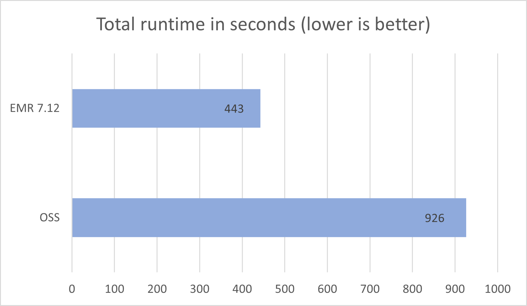
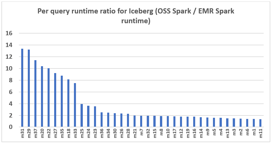
Apache Spark encryption performance improvement with Amazon EMR 7.9

Post Syndicated from Sonu Kumar Singh original https://aws.amazon.com/blogs/big-data/apache-spark-encryption-performance-improvement-with-amazon-emr-7-9/

The Amazon EMR runtime for Apache Spark is a performance-optimized runtime for Apache Spark that is 100% API compatible with open source Apache Spark. With Amazon EMR release 7.9.0, the EMR runtime for Apache Spark introduces significant performance improvements for encrypted workloads, supporting Spark version 3.5.5.

For compliance and security requirements, many customers need to enable Apache Spark’s local storage encryption (spark.io.encryption.enabled = true) in addition to Amazon Simple Storage Service (Amazon S3) encryption (such as server-side encryption (SSE) or AWS Key Management Service (AWS KMS)). This feature encrypts shuffle files, cached data, and other intermediate data written to local disk during Spark operations, protecting sensitive data at rest on Amazon EMR cluster instances.

Industries subject to regulations such as the Health Insurance Portability and Accountability Act (HIPAA) for healthcare, Payment Card Industry Data Security Standard (PCI-DSS) for financial services, General Data Protection Regulation (GDPR) for personal data, and Federal Risk and Authorization Management Program (FedRAMP) for government often require encryption of all data at rest, including temporary files on local storage. While Amazon S3 encryption protects data in object storage, Spark’s I/O encryption secures the intermediate shuffle and spill data that Spark writes to local disk during distributed processing—data that never reaches Amazon S3 but might contain sensitive information extracted from source datasets. Generally, encrypted operations require additional computational overhead that can impact overall job performance.

With the built-in encryption optimizations of Amazon EMR 7.9.0, customers might see significant performance improvements in their Apache Spark applications without requiring any application changes. In our performance benchmark tests, derived from TPC-DS performance tests at 3 TB scale, we observed up to 20% faster performance with the EMR 7.9 optimized Spark runtime compared to Spark without these optimizations. Individual results may vary depending on specific workloads and configurations.

In this post, we analyze the results from our benchmark tests comparing the Amazon EMR 7.9 optimized Spark runtime against Spark 3.5.5 without encryption optimizations. We walk through a detailed cost analysis and provide step-by-step instructions to reproduce the benchmark.

Results observed

To evaluate the performance improvements, we used an open source Spark performance test utility derived from the TPC-DS performance test toolkit. We ran the tests on two nine-node (eight core nodes and one primary node) r5d.4xlarge Amazon EMR 7.9.0 clusters, comparing two configurations:

  • Baseline: EMR 7.9.0 cluster with a bootstrap action installing Spark 3.5.5 without encryption optimizations
  • Optimized: EMR 7.9.0 cluster using the EMR Spark 3.5.5 runtime with encryption optimizations

Both tests used data stored in Amazon Simple Storage Service (Amazon S3). All data processing was configured identically except for the Spark runtime version.

To maintain benchmarking consistency and ensure a consistent, equivalent comparison, we disabled Dynamic Resource Allocation (DRA) in both test configurations. This approach eliminates variability from dynamic scaling and so we can measure pure computational performance improvements.

The following table shows the total job runtime for all queries (in seconds) in the 3 TB query dataset between the baseline and Amazon EMR 7.9 optimized configurations:

Configuration Total runtime (seconds) Geometric mean (seconds) Performance improvement
Baseline (Spark 3.5.5 without optimization) 1,485 10.24
EMR 7.9 (with encryption optimization) 1,176 8.15 20% faster

We observed that our TPC-DS tests with the Amazon EMR 7.9 optimized Spark runtime completed about 20% faster based on total runtime and 20% faster based on geometric mean compared to the baseline configuration.

The encryption optimizations in Amazon EMR 7.9 deliver performance benefits through:

  • Improved shuffle and decryption operations reducing overhead during data exchange without compromising security
  • Better memory management for intermediate results

Cost analysis

The performance improvements of the Amazon EMR 7.9 optimized Spark runtime directly translate to lower costs. We realized an approximately 20% cost savings running the benchmark application with encryption optimizations compared to the baseline configuration, because of reduced hours of EMR, Amazon Elastic Compute Cloud (Amazon EC2) and Amazon Elastic Block Store (Amazon EBS) using General Purpose SSD (gp2).

The following table summarizes the cost comparison in the us-east-1 AWS Region:

Configuration Runtime (hours) Estimated cost Total EC2 instances Total vCPU Total memory (GiB) Root device (EBS)
Baseline: Spark 3.5.5 without optimization, 1 primary and 8 core nodes 0.41 $5.28 9 144 1152 64 GiB gp2
Amazon EMR 7.9 with optimization, 1 primary and 8 core nodes 0.33 $4.25 9 144 1152 64 GiB gp2

Cost breakdown

Formulas used:

  • Amazon EMR cost – Number of instances × EMR hourly rate × Runtime hours
  • Amazon EC2 cost – Number of instances × EC2 hourly rate × Runtime hour)
  • Amazon EBS cost(EBS cost per GB per month ÷ hours in a month) × EBS volume size × number of instances × runtime hours

Note: EBS is priced monthly ($0.1 per GB per month), so we divide by 730 hours to convert to an hourly rate. EMR and EC2 are already priced hourly, so no conversion is needed.

Baseline configuration (0.41 hours):

  • Amazon EMR cost – 9 × $0.27 × 0.41 = $1.00
  • Amazon EC2 cost – 9 × $1.152 × 0.41 = $4.25
  • Amazon EBS cost – ($0.1/730 × 64 × 9 × 0.41) = $0.032
  • Total cost – $5.28

EMR 7.9 optimized configuration (0.33 hours):

  • Amazon EMR cost – (9 × $0.27 × 0.33) = $0.80
  • Amazon EC2 cost – (9 × $1.152 × 0.33) = $3.42
  • Amazon EBS cost – ($0.1/730 × 64 × 9 × 0.33) = $0.025
  • Total cost: $4.25

Total cost savings: 20% per benchmark run, which scales linearly with your production workload frequency.

Set up EMR benchmarking

For detailed instructions and scripts, see the companion GitHub repository.

Prerequisites

To set up Amazon EMR benchmarking, start by completing the following prerequisite steps:

  1. Configure your AWS Command Line Interface (AWS CLI) by running aws configure to point to your benchmarking account,
  2. Create an S3 bucket for test data and results.
  3. Copy the TPC-DS 3TB source data from a publicly available dataset to your S3 bucket using the following command:
    aws s3 cp s3://blogpost-sparkoneks-us-east-1/blog/BLOG_TPCDS-TEST-3T-partitioned s3://<YOUR-BUCKET-NAME>/BLOG_TPCDS-TEST-3T-partitioned --recursive

    Replace <YOUR-BUCKET-NAME> with the name of the S3 bucket you created in step 2.

  4. Build or download the benchmark application JAR file (spark-benchmark-assembly-3.3.0.jar)
  5. Ensure you have appropriate AWS Identity Access Management (IAM) roles for EMR cluster creation and Amazon S3 access

Deploy the baseline EMR cluster (without optimization)

Step 1: Launch EMR 7.9.0 cluster with bootstrap action

The baseline configuration uses a bootstrap action to install Spark 3.5.5 without encryption optimizations. We have made the bootstrap script publicly available in an S3 bucket for your convenience.

Create the default Amazon EMR roles:

aws emr create-default-roles

Now create the cluster:

aws emr create-cluster \
  --name "EMR-7.9-Baseline-Spark-3.5.5" \
  --release-label emr-7.9.0 \
  --applications Name=Spark \
  --ec2-attributes SubnetId=<YOUR-SUBNET-ID>,InstanceProfile=EMR_EC2_DefaultRole  \
  --service-role EMR_DefaultRole
  --instance-groups \
    InstanceGroupType=MASTER,InstanceCount=1,InstanceType=r5d.4xlarge \
    InstanceGroupType=CORE,InstanceCount=8,InstanceType=r5d.4xlarge \
  --bootstrap-actions \
    Path=s3://spark-ba/install-spark-3-5-5-no-encryption.sh,Name="install spark 3.5.5 without encryption optimization" \
  --use-default-roles \
  --log-uri s3://<YOUR-BUCKET-NAME>/logs/baseline/

Note: The bootstrap script is available in a public S3 bucket at s3://spark-ba/install-spark-3-5-5-no-encryption.sh. This script installs Apache Spark 3.5.5 without the encryption optimizations present in the Amazon EMR runtime.

Step 2: Submit the benchmark job to the baseline cluster

Next submit the Spark job using the following commands:

aws emr add-steps \
  --cluster-id <YOUR-BASELINE-CLUSTER-ID> \  
  --steps 'Type=Spark,Name="EMR-7.9-Baseline-Spark-3.5.5 Step",ActionOnFailure=CONTINUE,Args=["--deploy-mode","client","--conf","spark.io.encryption.enabled=false","--class","com.amazonaws.eks.tpcds.BenchmarkSQL","s3://<YOUR-BUCKET-NAME>/jar/spark-benchmark-assembly-3.3.0.jar","s3:// <YOUR-BUCKET-NAME>/blog/BLOG_TPCDS-TEST-3T-partitioned","s3:// <YOUR-BUCKET-NAME>/blog/BASELINE_TPCDS-TEST-3T-RESULT","/opt/tpcds-kit/tools","parquet","3000","3","false","q1-v2.4,q10-v2.4,q11-v2.4,q12-v2.4,q13-v2.4,q14a-v2.4,q14b-v2.4,q15-v2.4,q16-v2.4,q17-v2.4,q18-v2.4,q19-v2.4,q2-v2.4,q20-v2.4,q21-v2.4,q22-v2.4,q23a-v2.4,q23b-v2.4,q24a-v2.4,q24b-v2.4,q25-v2.4,q26-v2.4,q27-v2.4,q28-v2.4,q29-v2.4,q3-v2.4,q30-v2.4,q31-v2.4,q32-v2.4,q33-v2.4,q34-v2.4,q35-v2.4,q36-v2.4,q37-v2.4,q38-v2.4,q39a-v2.4,q39b-v2.4,q4-v2.4,q40-v2.4,q41-v2.4,q42-v2.4,q43-v2.4,q44-v2.4,q45-v2.4,q46-v2.4,q47-v2.4,q48-v2.4,q49-v2.4,q5-v2.4,q50-v2.4,q51-v2.4,q52-v2.4,q53-v2.4,q54-v2.4,q55-v2.4,q56-v2.4,q57-v2.4,q58-v2.4,q59-v2.4,q6-v2.4,q60-v2.4,q61-v2.4,q62-v2.4,q63-v2.4,q64-v2.4,q65-v2.4,q66-v2.4,q67-v2.4,q68-v2.4,q69-v2.4,q7-v2.4,q70-v2.4,q71-v2.4,q72-v2.4,q73-v2.4,q74-v2.4,q75-v2.4,q76-v2.4,q77-v2.4,q78-v2.4,q79-v2.4,q8-v2.4,q80-v2.4,q81-v2.4,q82-v2.4,q83-v2.4,q84-v2.4,q85-v2.4,q86-v2.4,q87-v2.4,q88-v2.4,q89-v2.4,q9-v2.4,q90-v2.4,q91-v2.4,q92-v2.4,q93-v2.4,q94-v2.4,q95-v2.4,q96-v2.4,q97-v2.4,q98-v2.4,q99-v2.4,ss_max-v2.4","true"]'

Deploy the optimized EMR cluster (with encryption optimization)

Step 1: Launch EMR 7.9.0 cluster with Spark runtime

The optimized configuration uses the EMR 7.9.0 Spark runtime without any bootstrap actions:

aws emr create-cluster \
  --name "EMR-7.9-Optimized-Native-Spark" \
  --release-label emr-7.9.0 \
  --applications Name=Spark \
  --ec2-attributes SubnetId=<YOUR-SUBNET-ID>,InstanceProfile=EMR_EC2_DefaultRole \
  --service-role EMR_DefaultRole
  --instance-groups \
    InstanceGroupType=MASTER,InstanceCount=1,InstanceType=r5d.4xlarge \
    InstanceGroupType=CORE,InstanceCount=8,InstanceType=r5d.4xlarge \
  --use-default-roles \
  --log-uri s3://<YOUR-BUCKET-NAME>/logs/optimized/

Example:

aws emr create-cluster \
--name "EMR-7.9-Optimized-Native-Spark" \
--release-label emr-7.9.0 \
--applications Name=Spark \
--ec2-attributes SubnetId=subnet-08a5f71f92bc8a801 \
--instance-groups \
InstanceGroupType=MASTER,InstanceCount=1,InstanceType=r5d.4xlarge \
InstanceGroupType=CORE,InstanceCount=8,InstanceType=r5d.4xlarge \
--bootstrap-actions \
Path=s3://spark-ba/install-spark-3-5-5-no-encryption.sh,Name="install spark 3.5.5 without encryption optimization" \
--use-default-roles \
--log-uri s3://aws-logs-123456789012-us-west-2/elasticmapreduce/

Step 2: Submit the benchmark job to optimized cluster

ext submit the Spark job using the following commands:

aws emr add-steps \
  --cluster-id <YOUR-OPTIMIZED-CLUSTER-ID> \ 
  --steps 'Type=Spark,Name="EMR-7.9-Optimized-Native-Spark Step",ActionOnFailure=CONTINUE,Args=["--deploy-mode","client","--conf","spark.io.encryption.enabled=true","--class","com.amazonaws.eks.tpcds.BenchmarkSQL","s3://<YOUR-BUCKET-NAME>/jar/spark-benchmark-assembly-3.3.0.jar","s3://<YOUR-BUCKET-NAME>/blog/BLOG_TPCDS-TEST-3T-partitioned","s3://<YOUR-BUCKET-NAME>/blog/BASELINE_TPCDS-TEST-3T-RESULT","/opt/tpcds-kit/tools","parquet","3000","3","false","q1-v2.4,q10-v2.4,q11-v2.4,q12-v2.4,q13-v2.4,q14a-v2.4,q14b-v2.4,q15-v2.4,q16-v2.4,q17-v2.4,q18-v2.4,q19-v2.4,q2-v2.4,q20-v2.4,q21-v2.4,q22-v2.4,q23a-v2.4,q23b-v2.4,q24a-v2.4,q24b-v2.4,q25-v2.4,q26-v2.4,q27-v2.4,q28-v2.4,q29-v2.4,q3-v2.4,q30-v2.4,q31-v2.4,q32-v2.4,q33-v2.4,q34-v2.4,q35-v2.4,q36-v2.4,q37-v2.4,q38-v2.4,q39a-v2.4,q39b-v2.4,q4-v2.4,q40-v2.4,q41-v2.4,q42-v2.4,q43-v2.4,q44-v2.4,q45-v2.4,q46-v2.4,q47-v2.4,q48-v2.4,q49-v2.4,q5-v2.4,q50-v2.4,q51-v2.4,q52-v2.4,q53-v2.4,q54-v2.4,q55-v2.4,q56-v2.4,q57-v2.4,q58-v2.4,q59-v2.4,q6-v2.4,q60-v2.4,q61-v2.4,q62-v2.4,q63-v2.4,q64-v2.4,q65-v2.4,q66-v2.4,q67-v2.4,q68-v2.4,q69-v2.4,q7-v2.4,q70-v2.4,q71-v2.4,q72-v2.4,q73-v2.4,q74-v2.4,q75-v2.4,q76-v2.4,q77-v2.4,q78-v2.4,q79-v2.4,q8-v2.4,q80-v2.4,q81-v2.4,q82-v2.4,q83-v2.4,q84-v2.4,q85-v2.4,q86-v2.4,q87-v2.4,q88-v2.4,q89-v2.4,q9-v2.4,q90-v2.4,q91-v2.4,q92-v2.4,q93-v2.4,q94-v2.4,q95-v2.4,q96-v2.4,q97-v2.4,q98-v2.4,q99-v2.4,ss_max-v2.4","true"]'

Benchmark command parameters explained

The Amazon EMR Spark step uses the following parameters:

  • EMR step configuration:
    • Type=Spark: Specifies this is a Spark application step
    • Name=”EMR-7.9-Baseline-Spark-3.5.5″: Human-readable name for the step
    • ActionOnFailure=CONTINUE: Continue with other steps if this one fails
  • Spark submit arguments:
    • –deploy-mode client: Run the driver on the master node (not cluster mode)
    • –class com.amazonaws.eks.tpcds.BenchmarkSQL: Main class for the TPC-DS benchmark
  • Application parameters:
    • JAR file: s3://<YOUR-BUCKET-NAME>/jar/spark-benchmark-assembly-3.3.0.jar
    • Input data: s3://<YOUR-BUCKET-NAME>/blog/BLOG_TPCDS-TEST-3T-partitioned (3 TB TPC-DS dataset)
    • Output location: s3://<YOUR-BUCKET-NAME>/blog/BASELINE_TPCDS-TEST-3T-RESULT (S3 path for results)
    • TPC-DS tools path: /opt/tpcds-kit/tools(local path on EMR nodes)
    • Format: parquet (output format)
    • Scale factor: 3000 (3 TB dataset size)
    • Iterations: 3 (run each query 3 times for averaging)
    • Collect results: false (don’t collect results to driver)
    • Query list: "q1-v2.4,q10-v2.4,...,ss_max-v2.4" (all 104 TPC-DS queries)
    • Final parameter: true (enable detailed logging and metrics)
  • Query coverage:
    • All 104 standard TPC-DS benchmark queries (q1-v2.4 through q99-v2.4)
    • Plus the ss_max-v2.4 query for additional testing
    • Each query runs 3 times to calculate average performance

Summarize the results

  1. Download the test result files from both output S3 locations:
    # Baseline results
    aws s3 cp s3://<YOUR-BUCKET-NAME>/blog/BASELINE_TPCDS-TEST-3T-RESULT/timestamp=xxxx/summary.csv/xxx.csv ./baseline-results.csv
       
    # Optimized results
    aws s3 cp s3://<YOUR-BUCKET-NAME>/blog/OPTIMIZED_TPCDS-TEST-3T-RESULT/timestamp=xxxx/summary.csv/xxx.csv ./optimized-results.csv

  2. The CSV files contain four columns (without headers):
    • Query name
    • Median time (seconds)
    • Minimum time (seconds)
    • Maximum time (seconds)
  3. Calculate performance metrics for comparison:
    • Average time per query: AVERAGE(median, min, max) for each query
    • Total runtime: Sum of all median times
    • Geometric mean: GEOMEAN(average times) across all queries
    • Speedup: Calculate the ratio between baseline and optimized for each query
  4. Create comparison analysis:Speedup = (Baseline Time - Optimized Time) / Baseline Time * 100%

Testing configuration details

The following table summarizes the test environment used for this post:

Parameter Value
EMR release emr-7.9.0 (both configurations)
Baseline Spark version 3.5.5 (installed through bootstrap action)
Baseline bootstrap script s3://spark-ba/install-spark-3-5-5-no-encryption.sh (public)
Optimized spark version Amazon EMR Spark runtime
Cluster size 9 nodes (1 primary and 8 core)
Instance type r5d.4xlarge
vCPUs per node 16
Memory per node 128 GB
Instance storage 600 GB SSD
EBS volume 64 GB gp2 (2 volumes per instance)
Total vCPUs 144 (9 × 16)
Total memory 1152 GB (9 × 128)
Dataset TPC-DS 3TB (Parquet format)
Queries 104 queries (TPC-DS v2.4)
Iterations 3 runs per query
DRA Disabled for consistent benchmarking

Clean up

To avoid incurring future charges, delete the resources you created:

  1. Terminate both EMR clusters:
    aws emr terminate-clusters --cluster-ids <YOUR-BASELINE-CLUSTER-ID> <YOUR-OPTIMIZED-CLUSTER-ID>

  2. Delete S3 test results if no longer needed:
    aws s3 rm s3://<YOUR-BUCKET-NAME>/blog/BASELINE_TPCDS-TEST-3T-RESULT/ --recursive
    aws s3 rm s3://<YOUR-BUCKET-NAME>/blog/OPTIMIZED_TPCDS-TEST-3T-RESULT/ --recursive
    aws s3 rm s3://<YOUR-BUCKET-NAME>/logs/ --recursive

  3. Remove IAM roles if created specifically for testing

Key findings

  • Up to 20% performance improvement using the Amazon EMR 7.9’s Spark runtime with no code changes required
  • 20% cost savings because of reduced runtime
  • Significant gains for shuffle-heavy, join-intensive workloads
  • 100% API compatibility with open source Apache Spark
  • Simple migration from custom Spark builds to EMR runtime
  • Easy benchmarking using publicly available bootstrap scripts

Conclusion

You can run your Apache Spark workloads up to 20% faster and at lower cost without making any changes to your applications by using the Amazon EMR 7.9.0 optimized Spark runtime. This improvement is achieved through numerous optimizations in the EMR Spark runtime, including enhanced encryption handling, improved data serialization, and optimized shuffle operations.

To learn more about Amazon EMR 7.9 and best practices, see the EMR documentation. For configuration guidance and tuning advice, subscribe to the AWS Big Data Blog.

Related resources:

If you’re running Spark workloads on Amazon EMR today, we encourage you to test the EMR 7.9 Spark runtime with your production workloads and measure the improvements specific to your use case.


About the authors

Sonu Kumar Singh

Sonu Kumar Singh

Sonu is a Senior Solutions Architect with more than 13 years of experience, with a specialization in Analytics and Healthcare domain. He has been instrumental in catalyzing transformative shifts in organizations by enabling data-driven decision-making thereby fueling innovation and growth. He enjoys it when something he designed or created brings a positive impact.

Roshin Babu

Roshin Babu

Roshin is a Sr. Specialist Solutions architect at AWS, where he collaborates with the sales team to support public sector clients. His role focuses on developing innovative solutions that solve complex business challenges while driving increased adoption of AWS analytics services. When he’s not working, Roshin is passionate about exploring new destinations, discovering great food, and enjoying soccer both as a player and fan.Polaris Jhandi

Polaris Jhandi

Polaris Jhandi

Polaris is a Cloud Application Architect with AWS Professional Services. He has a background in AI/ML and big data. He is currently working with customers to migrate their legacy mainframe applications to the AWS Cloud.Zheng Yuan

Zheng Yuan

Zheng Yuan

Zheng is a Software Engineer on the Amazon EMR Spark team, where he focuses on improving the performance of the Spark execution engine across various use cases.

Run Apache Spark and Apache Iceberg write jobs 2x faster with Amazon EMR

Post Syndicated from Atul Payapilly original https://aws.amazon.com/blogs/big-data/run-apache-spark-and-apache-iceberg-write-jobs-2x-faster-with-amazon-emr/

Amazon EMR runtime for Apache Spark offers a high-performance runtime environment while maintaining API compatibility with open source Apache Spark and Apache Iceberg table format. Amazon EMR on EC2, Amazon EMR Serverless, Amazon EMR on Amazon EKS, Amazon EMR on AWS Outposts and AWS Glue use the optimized runtimes.

In this post, we demonstrate the write performance benefits of using the Amazon EMR 7.12 runtime for Spark and Iceberg compares to open source Spark 3.5.6 with Iceberg 1.10.0 tables on a 3TB merge workload.

Write Benchmark Methodology

Our benchmarks demonstrate that Amazon EMR 7.12 can run 3TB merge workloads over 2 times faster than open source Spark 3.5.6 with Iceberg 1.10.0, delivering significant improvements for data ingestion and ETL pipelines while providing the advanced features of Iceberg including ACID transactions, time travel, and schema evolution.

Benchmark workload

To evaluate the write performance improvements in Amazon EMR 7.12, we chose a merge workload that reflects common data ingestion and ETL patterns. The benchmark consists of 37 basic merge operations on TPC-DS 3TB tables, testing the performance of INSERT, UPDATE, and DELETE operations. The workload is inspired by established benchmarking approaches from the open source community, including Delta Lake’s merge benchmark methodology and the LST-Bench framework. We combined and adapted these approaches to create a comprehensive test of Iceberg write performance on AWS. We also started with an initial focus on copy-on-write performance only.

Workload characteristics

The benchmark executes 37 basic sequential merge queries that modify TPC-DS fact tables. The 37 queries are organized into three categories:

  • Inserts (queries m1-m6): Adding new records to tables with varying data volumes. These queries use source tables with 5-100% new records and zero matches, testing pure insert performance at different scales.
  • Upserts (queries m8-m16): Modifying existing records while inserting new ones. These upsert operations combine different ratios of matched and non-matched records—for example, 1% matches with 10% inserts, or 99% matches with 1% inserts—representing typical scenarios where data is both updated and augmented.
  • Deletes (queries m7, m17-m37): Removing records with varying selectivity. These range from small, targeted deletes affecting 5% of files and rows to large-scale deletions, including partition-level deletes that can be optimized to metadata-only operations.

The queries operate on the table state created by previous operations, simulating real ETL pipelines where subsequent steps depend on earlier transformations. For example, the first six queries insert between 607,000 and 11.9 million records into the web_returns table. Later queries then update and delete from this modified table, testing read-after-write performance. Source tables were generated by sampling the TPC-DS web_returns table with controlled match/non-match ratios for consistent test conditions across the benchmark runs.

The merge operations vary in scale and complexity:

  • Small operations affecting 607,000 records
  • Large operations modifying over 12 million records
  • Selective deletes requiring file rewrites
  • Partition-level deletes optimized to metadata operations

Benchmark configuration

We ran the benchmark on identical hardware for both Amazon EMR 7.12 and open source Spark 3.5.6 with Iceberg 1.10.0:

  • Cluster: 9 r5d.4xlarge instances (1 primary, 8 workers)
  • Compute: 144 total vCPUs, 1,152 GB memory
  • Storage: 2 x 300 GB NVMe SSD per instance
  • Catalog: Hadoop Catalog
  • Data format: Parquet files on Amazon S3
  • Table format: Apache Iceberg (default: copy-on-write mode)

Benchmark results

We compared benchmark results for Amazon EMR 7.12 to open source Spark 3.5.6 and Iceberg 1.10.0. We ran the 37 merge queries in three sequential iterations, and the average runtime across these iterations was taken for comparison. The following table shows the results averaged across three iterations:

Amazon EMR 7.12 (seconds) Open Source Spark 3.5.6 + Iceberg 1.10.0 (seconds) Speedup
443.58 926.63 2.08x

The average runtime for the three iterations on Amazon EMR 7.12 with Iceberg enabled was 443.58 seconds, demonstrating a 2.08x speed increase compared to open source Spark 3.5.6 and Iceberg 1.10.0. The following figure presents the total runtimes in seconds.

The following table summarizes the metrics.

Metric Amazon EMR 7.12 on EC2 Open source Spark 3.5.6 and Iceberg 1.10.0
Average runtime in seconds 443.58 926.63
Geometric mean over queries in seconds 6.40746 18.50945
Cost* $1.58 $2.68

*Detailed cost estimates are discussed later in this post.

The following chart demonstrates the per-query performance improvement of Amazon EMR 7.12 relative to open source Spark 3.5.6 and Iceberg 1.10.0. The extent of the speedup varies from one query to another, with the fastest up to 13.3 times faster for query m31, with Amazon EMR outperforming open source Spark with Iceberg tables. The horizontal axis arranges the TPC-DS 3TB benchmark queries in descending order based on the performance improvement seen with Amazon EMR, and the vertical axis depicts the magnitude of this speedup as a ratio.

Performance optimizations in Amazon EMR

Amazon EMR 7.12 achieves over 2x faster write performance through systematic optimizations across the write execution pipeline. These improvements span multiple areas:

  • Metadata-only delete operations: When deleting entire partitions, EMR can now optimize these operations to metadata-only changes, eliminating the need to rewrite data files. This significantly reduces the time and cost for partition-level delete operations.
  • Bloom filter joins for merge operations: Enhanced join strategies using bloom filters reduce the amount of data that needs to be read and processed during merge operations, particularly benefiting queries with selective predicates.
  • Parallel file write out: Optimized parallelism during the write phase of merge operations improves throughput when writing filtered results back to Amazon S3, reducing overall merge operation time. We balanced the parallelism with read performance for overall optimized performance on the entire workload.

These optimizations work together to deliver consistent performance improvements across diverse write patterns. The result is significantly faster data ingestion and ETL pipeline execution while maintaining Iceberg’s ACID assurances and data consistency of Iceberg.

Cost comparison

Our benchmark provides the total runtime and geometric mean data to assess the performance of Spark and Iceberg in a complex, real-world decision support scenario. For additional insights, we also examine the cost aspect. We calculate cost estimates using formulas that account for EC2 On-Demand instances, Amazon Elastic Block Store (Amazon EBS), and Amazon EMR expenses.

  • Amazon EC2 cost (includes SSD cost) = number of instances * r5d.4xlarge hourly rate * job runtime in hours
    • 4xlarge hourly rate = $1.152 per hour
  • Root Amazon EBS cost = number of instances * Amazon EBS per GB-hourly rate * root EBS volume size * job runtime in hours
  • Amazon EMR cost = number of instances * r5d.4xlarge Amazon EMR cost * job runtime in hours
    • 4xlarge Amazon EMR cost = $0.27 per hour
  • Total cost = Amazon EC2 cost + root Amazon EBS cost + Amazon EMR cost

The calculations reveal that the Amazon EMR 7.12 benchmark yields a 1.7x cost efficiency improvement over open source Spark 3.5.6 and Iceberg 1.10.0 in running the benchmark job.

Metric Amazon EMR 7.12 Open source Spark 3.5.6 and Iceberg 1.10.0
Runtime in seconds 443.58 926.63
Number of EC2 instances(Includes primary node) 9 9
Amazon EBS Size 20gb 20gb
Amazon EC2(Total runtime cost) $1.28 $2.67
Amazon EBS cost $0.00 $0.01
Amazon EMR cost $0.30 $0
Total cost $1.58 $2.68
Cost savings Amazon EMR 7.12 is 1.7 times better Baseline

Run open source Spark benchmarks on Iceberg tables

We used separate EC2 clusters, each equipped with nine r5d.4xlarge instances, for testing both open source Spark 3.5.6 and Amazon EMR 7.12 for Iceberg workload. The primary node was equipped with 16 vCPU and 128 GB of memory, and the eight worker nodes together had 128 vCPU and 1024 GB of memory. We conducted tests using the Amazon EMR default settings to showcase the typical user experience and minimally adjusted the settings of Spark and Iceberg to maintain a balanced comparison.

The following table summarizes the Amazon EC2 configurations for the primary node and eight worker nodes of type r5d.4xlarge.

EC2 Instance vCPU Memory (GiB) Instance storage (GB) EBS root volume (GB)
r5d.4xlarge 16 128 2 x 300 NVMe SSD 20 GB

Benchmarking instructions

Follow the steps below to run the benchmark:

  1. For the open source run, create a Spark cluster on Amazon EC2 using Flintrock with the configuration described previously.
  2. Setup the TPC-DS source data with Iceberg in your S3 bucket.
  3. Build the benchmark application jar from the source to run the benchmarking and get the results.

Detailed instructions are provided in the emr-spark-benchmark GitHub repository.

Summarize the results

After the Spark job finishes, retrieve the test result file from the output S3 bucket at s3://<YOUR_S3_BUCKET>/benchmark_run/timestamp=xxxx/summary.csv/xxx.csv. This can be done either through the Amazon S3 console by navigating to the specified bucket location or by using the Amazon Command Line Interface (AWS CLI). The Spark benchmark application organizes the data by creating a timestamp folder and placing a summary file within a folder labeled summary.csv. The output CSV files contain four columns without headers:

  • Query name
  • Median time
  • Minimum time
  • Maximum time

With the data from three separate test runs with one iteration each time, we can calculate the average and geometric mean of the benchmark runtimes.

Clean up

To help prevent future charges, delete the resources you created by following the instructions provided in the Cleanup section of the GitHub repository.

Summary

Amazon EMR is consistently enhancing the EMR runtime for Spark when used with Iceberg tables, achieving write performance that is over 2 times faster than open source Spark 3.5.6 and Iceberg 1.10.0 with EMR 7.12 on 3TB merge workloads. This represents a significant improvement for data ingestion and ETL pipelines, helping to deliver 1.7x cost reduction while maintaining the ACID assurances of Iceberg. We encourage you to keep up to date with the latest Amazon EMR releases to fully benefit from ongoing performance improvements.

To stay informed, subscribe to the RSS feed for the AWS Big Data Blog, where you can find updates on the EMR runtime for Spark and Iceberg, as well as tips on configuration best practices and tuning recommendations.


About the authors

Atul Felix Payapilly is a software development engineer for Amazon EMR at Amazon Web Services.

Akshaya KP is a software development engineer for Amazon EMR at Amazon Web Services.

Hari Kishore Chaparala is a software development engineer for Amazon EMR at Amazon Web Services.

Giovanni Matteo is the Senior Manager for the Amazon EMR Spark and Iceberg group.

Accelerate data lake operations with Apache Iceberg V3 deletion vectors and row lineage

Post Syndicated from Ron Ortloff original https://aws.amazon.com/blogs/big-data/accelerate-data-lake-operations-with-apache-iceberg-v3-deletion-vectors-and-row-lineage/

Organizations building petabyte-scale data lakes face increasing challenges as their data grows. Batch updates and compliance deletes create a proliferation of positional delete files, slowing downstream data pipelines and driving up storage costs. Tracking data changes for audit trails and incremental processing requires custom, engine-specific implementations that add complexity and maintenance burden. As data volumes scale, these challenges compound, leaving data teams juggling custom solutions and increasing operational costs just to maintain data freshness and compliance.

Apache Iceberg V3 addresses these challenges with two new capabilities: deletion vectors and row lineage. AWS now delivers these capabilities across Apache Spark on Amazon EMR 7.12, AWS Glue, Amazon SageMaker notebooks, Amazon S3 Tables, and the AWS Glue Data Catalog, giving you a complete, integrated V3 experience without custom implementation. This means faster writes, lower storage costs, comprehensive audit trails, and efficient incremental processing, all working seamlessly across your entire data lake architecture.

In this post, we walk you through the new capabilities in Iceberg V3, explain how deletion vectors and row lineage address these challenges, explore real-world use cases across industries, and provide practical guidance on implementing Iceberg V3 features across AWS analytics, catalog, and storage services.

What’s new in Iceberg V3

Iceberg V3 introduces new capabilities and data types. Two key capabilities that address the challenges discussed earlier are deletion vectors and row lineage.

Deletion vectors replace positional delete files with an efficient binary format stored as Puffin files. Instead of creating separate delete files for each delete operation, the deletion vector consolidates these delete references to a single delete vector per data file, rather than a delete reference file per deleted row. During query execution, engines efficiently filter out deleted rows using these compact vectors, maintaining query performance while removing the need to merge multiple delete files.

This avoids write amplification from random batch updates and GDPR compliance deletes, significantly reducing the overhead of maintaining fresh data. High-frequency update workloads can see immediate improvements in write performance and reduced storage costs from fewer small delete files. Additionally, having fewer small delete files reduces table maintenance costs for compaction operations.

Row lineage enables precise change tracking at the row level with full auditability. Row lineage adds metadata fields to each data file that track when rows were created and last modified. The _row_id field uniquely identifies each row, and the _last_updated_sequence_number field tracks the snapshot when the row was last modified. These fields enable efficient change tracking queries without scanning entire tables, and they’re automatically maintained by the Iceberg specification without requiring custom code.

Before row lineage, change tracking in Iceberg provided only the net changes between snapshots, making it difficult to track individual record modifications. Row lineage metadata fields can now be queried to return all incremental changes, giving you full fidelity for auditing data modifications and regulatory compliance. For data transformations, your downstream systems can process changes incrementally, speeding up data pipelines and reducing compute costs for change data capture (CDC) workflows. Row lineage is engine agnostic, interoperable, and built into the Iceberg V3 specification, alleviating the need for custom, engine-specific change tracking implementations.

Real-world use cases

The new Iceberg V3 capabilities address critical challenges across multiple industries:

  • Marketing and advertising services organizations – You can now efficiently handle GDPR right-to-be-forgotten requests and regulatory compliance deletes without the write amplification that previously degraded pipeline performance. Row lineage provides complete audit trails for data modifications, meeting strict regulatory requirements for data governance.
  • Ecommerce platforms processing millions of product updates and inventory changes daily – You can maintain data freshness while reducing storage costs. Deletion vectors enable faster upsert operations, helping teams meet aggressive SLA requirements during peak shopping periods.
  • Healthcare and life sciences companies – You can track patient data modifications with precision for compliance purposes while efficiently processing large-scale genomic datasets. Row lineage provides the detailed change history required for clinical trial audits and regulatory submissions.
  • Media and entertainment providers managing large catalogs of user viewing data – You can efficiently process incremental changes for recommendation engines. Row lineage enables downstream analytics systems to process only changed records, reducing compute costs in incremental processing scenarios.

Get started with Iceberg V3

To take advantage of deletion vectors for optimized writes and row lineage for built-in change tracking in Iceberg V3, set the table property format-version = 3 during table creation. Alternatively, setting this property on an existing Iceberg V2 table atomically upgrades the table without data rewrites. Before creating or upgrading V3 tables, make sure the Iceberg engines in your solution are V3-compatible. Refer to Apache Iceberg V3 on AWS for more details.

Create a new V3 table with Apache Spark on Amazon EMR 7.12

The following code creates a new table named customer_data. Setting the table property format-version = 3 creates a V3 table. If the format-version table property is not explicitly set, a V2 table is created. V2 is currently the Iceberg default table version. Setting write.delete.mode, write.update.mode, and write.merge.mode to merge-on-read configures Spark to write deletion vectors for delete, update, or merge statements performed on the table.

CREATE TABLE customer_data (
customer_id bigint,
name string,
email string,
last_purchase timestamp,
total_spent decimal(10,2)
)
USING iceberg
TBLPROPERTIES (
'format-version' = '3',
'write.delete.mode' = 'merge-on-read',
'write.update.mode' = 'merge-on-read',
'write.merge.mode' = 'merge-on-read'
)

Run the following code to insert records into the customer_data table:

INSERT INTO customer_data VALUES
 (1, 'Alejandro Rosalez', '[email protected]', TIMESTAMP '2025-11-24 18:55:27', 42.97)
,(2, 'Akua Mansa', '[email protected]', TIMESTAMP '2025-11-24 17:55:27', 25.02)
,(3, 'Ana Carolina Silva','[email protected]', TIMESTAMP '2025-11-24 16:55:27', 43.67)
,(4, 'Arnav Desai','[email protected]', TIMESTAMP '2025-11-24 15:55:27', 98.32)
,(5, 'Carlos Salazar','[email protected]', TIMESTAMP '2025-11-24 12:55:27', 76.45)

Delete a record where customer_id = 5 to generate a delete file:

DELETE 
  FROM customer_data 
  WHERE customer_id = 5

Updating a record with the following update statement also generates a delete file:

UPDATE customer_data
  SET name = 'Mansa Akua' 
  WHERE customer_id = 2

The last part of this example queries the manifest’s metadata table to verify delete files were produced:

SELECT added_snapshot_id
      ,sum(added_delete_files_count) as added_delete_files_count 
FROM customer_data.manifests 
GROUP BY added_snapshot_id 
ORDER BY added_snapshot_id

This query will result in three records returned, as shown in the following screenshot. The added_delete_files_count for the first snapshot that inserts records should be 0. The next two snapshots for the corresponding delete and update statements should have 1 each for added_delete_files_count value.

Query row lineage for change tracking

Row lineage is automatically enabled on V3 tables. The following example includes row lineage metadata fields and an example of how to query table changes after a row lineage sequence number:

SELECT
customer_id,
name,
email,
_row_id,
_last_updated_sequence_number
FROM customer_data
WHERE _last_updated_sequence_number > 0
ORDER BY _last_updated_sequence_number, _row_id

Running this query after the previous insert, update, and delete statements returns four records, as shown in the following screenshot. The deleted record is removed. The _last_updated_sequence_number is 3 for the update to customer_id = 2.

Upgrade an existing V2 table

You can upgrade your existing V2 tables to V3 with the following command:

ALTER TABLE existing_customer_data
SET TBLPROPERTIES ('format-version' = '3')

When you upgrade a table from V2 to V3, several important operations occur atomically:

  • A new metadata snapshot is created atomically, resulting in no data loss.
  • Existing Parquet data files are reused without modification.
  • Row-lineage fields (_row_id and _last_updated_sequence_number) are added to the table metadata.
  • The next compaction operation will remove old V2 positional delete files. If new deletion vector files are generated before compaction runs, they will merge existing V2 positional delete files.
  • New modifications will automatically use V3’s deletion vector files.
  • The upgrade does not perform a historical backfill of row-lineage change tracking records.

The upgrade process is synchronous and completes in seconds for most tables. If the upgrade fails, an error message is returned immediately, and the table remains in its V2 state.

Getting the most from Iceberg V3

In this section, we share the key things we’ve learned from customers already using these features.

Know your workload pattern

Deletion vectors work best when you’re doing lots of writes, such as high-frequency updates, batch deletes, or CDC workloads making random non-append-only updates. If you’re writing more than you’re reading, deletion vectors will deliver immediate performance gains. To unlock these benefits, set your table to merge-on-read mode for delete, update, and merge operations.

Let AWS handle compaction

Enable automatic compaction through the Data Catalog or use S3 Tables (on by default). You will get hands-free optimization without building custom maintenance jobs. Deletion vectors produce fewer delete files than positional deletes in Iceberg V2. Given a similar pattern and amount of modified records, V3 compaction should be quicker and cost less than V2.

Understand the importance of row lineage when using the V2 changelog

With the Spark changelog procedure in Iceberg V2, if a row gets inserted and then deleted between snapshots, it disappears from your change feed—you never see it. Iceberg V3 row lineage captures both operations because _last_updated_sequence_number updates on each modification. This full fidelity is important for audit trails and regulatory compliance where you need to prove what happened to every record. Performance-wise, the V2 changelog requires scanning and merging delete files to compute changes—that’s compute you’re paying for on every read. V3 row lineage stores metadata fields directly on each row, so filtering by _last_updated_sequence_number is a simple metadata scan.

Test before you upgrade

Iceberg V3 upgrades are atomic and fast, but test in dev first. Make sure all your query engines support Iceberg V3 before upgrading shared tables—mixing V2 and V3 engines causes headaches. After upgrading, keep a few V2 snapshots around temporarily for time-travel queries while you validate performance.

Conclusion

Iceberg V3 support across AWS analytics, catalog, and storage services marks a significant advancement in data lake capabilities. By combining deletion vectors’ write optimization with row lineage’s comprehensive change tracking, you can build more efficient, auditable, and cost-effective data lakes at scale. The seamless interoperability across AWS services makes sure your data lake architecture remains flexible and future-proof.

To learn more about AWS support for Iceberg V3, refer to Using Apache Iceberg on AWS.

To learn more about building modern data lakes with Iceberg on AWS, refer to Analytics on AWS.


About the authors

Ron Ortloff

Ron Ortloff

Ron is a Principal Product Manager at AWS.

Visualize data lineage using Amazon SageMaker Catalog for Amazon EMR, AWS Glue, and Amazon Redshift

Post Syndicated from Shubham Purwar original https://aws.amazon.com/blogs/big-data/visualize-data-lineage-using-amazon-sagemaker-catalog-for-amazon-emr-aws-glue-and-amazon-redshift/

Amazon SageMaker offers a comprehensive hub that integrates data, analytics, and AI capabilities, providing a unified experience for users to access and work with their data. Through Amazon SageMaker Unified Studio, a single and unified environment, you can use a wide range of tools and features to support your data and AI development needs, including data processing, SQL analytics, model development, training, inference, and generative AI development. This offering is further enhanced by the integration of Amazon Q and Amazon SageMaker Catalog, which provide an embedded generative AI and governance experience, helping users work efficiently and effectively across the entire data and AI lifecycle, from data preparation to model deployment and monitoring.

With the SageMaker Catalog data lineage feature, you can visually track and understand the flow of your data across different systems and teams, gaining a complete picture of your data assets and how they’re connected. As an OpenLineage-compatible feature, it helps you trace data origins, track transformations, and view cross-organizational data consumption, giving you insights into cataloged assets, subscribers, and external activities. By capturing lineage events from OpenLineage-enabled systems or through APIs, you can gain a deeper understanding of your data’s journey, including activities within SageMaker Catalog and beyond, ultimately driving better data governance, quality, and collaboration across your organization.

Additionally, the SageMaker Catalog data lineage feature versions each event, so you can track changes, visualize historical lineage, and compare transformations over time. This provides valuable insights into data evolution, facilitating troubleshooting, auditing, and data integrity by showing exactly how data assets have evolved, and generates trust in data.

In this post, we discuss the visualization of data lineage in SageMaker Catalog and how capture lineage from different AWS analytics services such as AWS Glue, Amazon Redshift, and Amazon EMR Serverless automatically, and visualize it with SageMaker Unified Studio.

Solution overview

The generation of data lineage in SageMaker Catalog operates through an automated system that captures metadata and relationships between different data artifacts for AWS Glue, Amazon EMR, and Amazon Redshift. When data moves through various AWS services, SageMaker automatically tracks these movements, transformations, and dependencies, creating a detailed map of the data’s journey. This tracking includes information about data sources, transformations, processing steps, and final outputs, providing a complete audit trail of data movement and transformation.

The implementation of data lineage in SageMaker Catalog offers several key benefits:

  • Compliance and audit support – Organizations can demonstrate compliance with regulatory requirements by showing complete data provenance and transformation history
  • Impact analysis – Teams can assess the potential impact of changes to data sources or transformations by understanding dependencies and relationships in the data pipeline
  • Troubleshooting and debugging – When issues arise, the lineage system helps identify the root cause by showing the complete path of data transformation and processing
  • Data quality management – By tracking transformations and dependencies, organizations can better maintain data quality and understand how data quality issues might propagate through their systems

Lineage capture is automated using several tools in SageMaker Unified Studio. To learn more, refer to Data lineage support matrix.

In the following sections, we show you how to configure your resources and implement the solution. For this post, we create the solution resources in the us-west-2 AWS Region using an AWS CloudFormation template.

Prerequisites

Before getting started, make sure you have the following:

Configure SageMaker Unified Studio with AWS CloudFormation

The vpc-analytics-lineage-sus.yaml stack creates a VPC, subnet, security group, IAM roles, NAT gateway, internet gateway, Amazon Elastic Compute Cloud (Amazon EC2) client, S3 buckets, SageMaker Unified Studio domain, and SageMaker Unified Studio project. To create the solution resources, complete the following steps:

  1. Launch the stack vpc-analytics-lineage-sus using the CloudFormation template:
  2. Provide the parameter values as listed in the following table.

    Parameters Sample value
    DatazoneS3Bucket s3://datazone-{account_id}/
    DomainName dz-studio
    EnvironmentName sm-unifiedstudio
    PrivateSubnet1CIDR 10.192.20.0/24
    PrivateSubnet2CIDR 10.192.21.0/24
    PrivateSubnet3CIDR 10.192.22.0/24
    ProjectName sidproject
    PublicSubnet1CIDR 10.192.10.0/24
    PublicSubnet2CIDR 10.192.11.0/24
    PublicSubnet3CIDR 10.192.12.0/24
    UsersList analyst
    VpcCIDR 10.192.0.0/16

The stack creation process can take approximately 20 minutes to complete. You can check the Outputs tab for the stack after the stack is created.

Next, we prepare source data, setup the AWS Glue ETL Job, Amazon EMR Serverless Spark Job and Amazon Redshift Job to generate the lineage and capture lineage from Amazon SageMaker Unified Studio

Prepare data

The following is example data from our CSV files:

attendance.csv

EmployeeID,Date,ShiftStart,ShiftEnd,Absent,OvertimeHours
E1000,2024-01-01,2024-01-01 08:00:00,2024-01-01 16:22:00,False,3
E1001,2024-01-08,2024-01-08 08:00:00,2024-01-08 16:38:00,False,2
E1002,2024-01-23,2024-01-23 08:00:00,2024-01-23 16:24:00,False,3
E1003,2024-01-09,2024-01-09 10:00:00,2024-01-09 18:31:00,False,0
E1004,2024-01-15,2024-01-15 09:00:00,2024-01-15 17:48:00,False,1

employees.csv

EmployeeID,Name,Department,Role,HireDate,Salary,PerformanceRating,Shift,Location
E1000,Employee_0,Quality Control,Operator,2021-08-08,33002.0,1,Night,Plant C
E1001,Employee_1,Maintenance,Supervisor,2015-12-31,69813.76,5,Evening,Plant B
E1002,Employee_2,Production,Technician,2015-06-18,46753.32,1,Evening,Plant A
E1003,Employee_3,Admin,Supervisor,2020-10-13,52853.4,5,Night,Plant A
E1004,Employee_4,Quality Control,Manager,2023-09-21,55645.27,5,Evening,Plant A

Upload the sample data from attendance.csv and employees.csv to the S3 bucket specified in the previous CloudFormation stack (s3://datazone-{account_id}/csv/).

Ingest employee data in Amazon Relational Database Dervice (Amazon RDS) for MySQL table

On the CloudFormation console, open the stack vpc-analytics-lineage-sus and collect the Amazon RDS for MySQL database endpoint to use in the following commands to create a default employeedb database.

  1. Connect to Amazon EC2 instance with mysql package installation
  2. Run the following command to connect to the database
    >MySQL -u admin -h database-1.cuqd06l5efvw.us-west-2.rds.amazonaws.com -p

  3. Run the following command to create an employee table
    Use employeedb;
    
    CREATE TABLE employee (
      EmployeeID longtext,
      Name longtext,
      Department longtext,
      Role longtext,
      HireDate longtext,
      Salary longtext,
      PerformanceRating longtext,
      Shift longtext,
      Location longtext
    );

  4. Running the following command to insert rows.
    INSERT INTO employee (EmployeeID, Name, Department, Role, HireDate, Salary, PerformanceRating, Shift, Location) VALUES ('E1000', 'Employee_0', 'Quality Control', 'Operator', '2021-08-08', 33002.00, 1, 'Night', 'Plant C'), ('E1001', 'Employee_1', 'Maintenance', 'Supervisor', '2015-12-31', 69813.76, 5, 'Evening', 'Plant B'), ('E1002', 'Employee_2', 'Production', 'Technician', '2015-06-18', 46753.32, 1, 'Evening', 'Plant A'), ('E1003', 'Employee_3', 'Admin', 'Supervisor', '2020-10-13', 52853.40, 5, 'Night', 'Plant A'), ('E1004', 'Employee_4', 'Quality Control', 'Manager', '2023-09-21', 55645.27, 5, 'Evening', 'Plant A');

Capture lineage from AWS Glue ETL job and notebook

To demonstrate the lineage, we set up an AWS Glue extract, transform, and load (ETL) job to read the employee data from an Amazon RDS for MySQL table and the employee attendance data from Amazon S3, and join both datasets. Finally, we write the data to Amazon S3 and create the attendance_with_emp1 table in the AWS Glue Data Catalog.

Create and configure AWS Glue job for lineage generation

Complete the following steps to create your AWS Glue ETL job:

  1. On the AWS Glue console, create a new ETL job with AWS Glue version 5.0.
  2. Enable Generate lineage events and provide the domain ID (retrieve from the CloudFormation template output for DataZoneDomainid; it will have the format dzd_xxxxxxxx)
  3. Use the following code snippet in the AWS Glue ETL job script. Provide the S3 bucket (bucketname-{account_id}) used in the preceding CloudFormation stack.
    from pyspark.sql import SparkSession
    from pyspark.sql import SparkSession, DataFrame
    from pyspark.sql.functions import *
    from pyspark.sql.types import *
    from pyspark import SparkContext
    from pyspark.sql import SparkSession
    import sys
    import logging
    
    
    spark = SparkSession.builder.appName("lineageglue").enableHiveSupport().getOrCreate()
     
    connection_details = glueContext.extract_jdbc_conf(connection_name="connectionname")
    
    employee_df = spark.read.format("jdbc").option("url", "jdbc:MySQL://dbhost:3306/database_name").option("dbtable", "employee").option("user", connection_details['user']).option("password", connection_details['password']).load()
    
    s3_paths = {
    'absent_data': 's3://bucketname-{account_id}/csv/attendance.csv'
    }
    absent_df = spark.read.csv(s3_paths['absent_data'], header=True, inferSchema=True)
    
    joined_df = employee_df.join(absent_df, on="EmployeeID", how="inner")
    
    joined_df.write.mode("overwrite").format("parquet").option("path", "s3://datazone-{account_id}/attendanceparquet/").saveAsTable("gluedbname.tablename")

  4. Choose Run to start the job.
  5. On the Runs tab, confirm the job ran without failure.
  6. After the job has executed successfully, navigate to the SageMaker Unified Studio domain.
  7. Choose Project and under Overview, choose Data Sources.
  8. Select the Data Catalog source (accountid-AwsDataCatalog-glue_db_suffix-default-datasource).
  9. On the Actions dropdown menu, choose Edit.
  10. Under Connection, enable Import data lineage.
  11. In the Data Selection section, under Table Selection Criteria, provide a table name or use * to generate lineage.
  12. Update the data source and choose Run to create an asset called attendance_with_emp1 in SageMaker Catalog.
  13. Navigate to Assets, choose the attendance_with_emp1 asset, and navigate to the LINEAGE section.

The following lineage diagram shows an AWS Glue job that integrates data from two sources: employee information stored in Amazon RDS for MySQL and employee absence records stored in Amazon S3. The AWS Glue job combines these datasets through a join operation, then creates a table in the Data Catalog and registers it as an asset in SageMaker Catalog, making the unified data available for further analysis or machine learning purposes.

Create and configure AWS Glue notebook for lineage generation

Complete the following steps to create the AWS Glue notebook:

  1. On the AWS Glue console, choose Author using an interactive code notebook.
  2. Under Options, choose Start fresh and choose Create notebook.
  3. In the notebook, use the following code to generate lineage.

    In the following code, we add the required Spark configuration to generate lineage and then read CSV data from Amazon S3 and write in Parquet format to the Data Catalog table. The Spark configuration includes the following parameters:

    • spark.extraListeners=io.openlineage.spark.agent.OpenLineageSparkListener – Registers the OpenLineage listener to capture Spark job execution events and metadata for lineage tracking
    • spark.openlineage.transport.type=amazon_datazone_api – Specifies Amazon DataZone as the destination service where the lineage data will be sent and stored
    • spark.openlineage.transport.domainId=dzd_xxxxxxx – Defines the unique identifier of your Amazon DataZone domain where the lineage data will be associated
    • spark.glue.accountId={account_id} – Specifies the AWS account ID where the AWS Glue job is running for proper resource identification and access
    • spark.openlineage.facets.custom_environment_variables – Lists the specific environment variables to capture in the lineage data for context about the AWS and AWS Glue environment
    • spark.glue.JOB_NAME=lineagenotebook – Sets a unique identifier name for the AWS Glue job that will appear in lineage tracking and logs

    See the following code:

    %%configure —name project.spark -f
    {
    "—conf":"spark.extraListeners=io.openlineage.spark.agent.OpenLineageSparkListener \
    --conf spark.openlineage.transport.type=amazon_datazone_api \
    --conf spark.openlineage.transport.domainId=dzd_xxxxxxxx \
    --conf spark.glue.accountId={account_id} \
    --conf spark.openlineage.facets.custom_environment_variables=[AWS_DEFAULT_REGION;GLUE_VERSION;GLUE_COMMAND_CRITERIA;GLUE_PYTHON_VERSION;] \
    --conf spark.glue.JOB_NAME=lineagenotebook"
    }
    
    from pyspark.sql import SparkSession
    from pyspark.sql import SparkSession, DataFrame
    from pyspark.sql.functions import *
    from pyspark.sql.types import *
    from pyspark import SparkContext
    from pyspark.sql import SparkSession
    import sys
    import logging
    
    
    spark = SparkSession.builder.appName("lineagegluenotebook").enableHiveSupport().getOrCreate()
    
    s3_paths = {
    'absent_data': 's3://datazone-{account_id}/csv/attendance.csv'
    }
    absent_df = spark.read.csv(s3_paths['absent_data'], header=True, inferSchema=True)
    
    absent_df.write.mode("overwrite").format("parquet").option("path", "s3://datazone-{account_id}/attendanceparquet2/").saveAsTable("gluedbname.tablename")

  4. After the notebook has executed successfully, navigate to the SageMaker Unified Studio domain.
  5. Choose Project and under Overview, choose Data Sources.
  6. Choose the Data Catalog source ({account_id}-AwsDataCatalog-glue_db_suffix-default-datasource).
  7. Choose Run to create the asset attendance_with_empnote in SageMaker Catalog.
  8. Navigate to Assets, choose the attendance_with_empnote asset, and navigate to the LINEAGE section.

The following lineage diagram shows an AWS Glue job that reads data from the employee absence records stored in Amazon S3. The AWS Glue job transform CSV data into Parquet format, then creates a table in the Data Catalog and registers it as an asset in SageMaker Catalog.

Capture lineage from Amazon Redshift

To demonstrate the lineage, we are creating an employee table and an attendance table and join both datasets. Finally, we create a new table called employeewithabsent in Amazon Redshift. Complete the following steps to create and configure lineage for Amazon Redshift tables:

  1. In SageMaker Unified Studio, open your domain.
  2. Under Compute, choose Data warehouse.
  3. Open project.redshift and copy the endpoint name (redshift-serverless-workgroup-xxxxxxx).
  4. On the Amazon Redshift console, open the Query Editor v2, and connect to the Redshift Serverless workgroup with a secret. Use the AWS Secrets Manager option and choose the secret redshift-serverless-namespace-xxxxxxxx.
  5. Use the following code to create tables in Amazon Redshift and load data from Amazon S3 using the COPY command. Make sure the IAM role has GetObject permission on the S3 files attendance.csv and employees.csv.

    Create Redshift table absent

    CREATE TABLE public.absent (
        employeeid character varying(65535),
        date date,
        shiftstart timestamp without time zone ,
        shiftend timestamp without time zone,
        absent boolean,
        overtimehours integer
    );

    Load data into absent table.

    COPY absent
    FROM 's3://datazone-{account_id}/csv/attendance.csv' 
    IAM_ROLE 'arn:aws:iam::accountid:role/RedshiftAdmin'
    csv
    IGNOREHEADER 1;

    Create Redshift table employee

    CREATE TABLE public.employee (
        employeeid character varying(65535),
        name character varying(65535),
        department character varying(65535),
        role character varying(65535),
        hiredate date,
        salary double precision,
        performancerating integer,
        shift character varying(65535),
        location character varying(65535)
    );

    Load data into employee table.

    COPY employee
    FROM 's3://datazone-{account_id}/csv/employees.csv' 
    IAM_ROLE 'arn:aws:iam::account-id:role/RedshiftAdmin'
    csv
    IGNOREHEADER 1;

  6. After the tables are created and the data is loaded, perform the join between the tables and create a new table with a CTAS query:
    CREATE TABLE public.employeewithabsent AS
    SELECT 
      e.*,
      a.absent,
      a.overtimehours
    FROM public.employee e
    INNER JOIN public.absent a
    ON e.EmployeeID = a.EmployeeID;

  7. Navigate to the SageMaker Unified Studio domain.
  8. Choose Project and under Overview, choose Data Sources.
  9. Select the Amazon Redshift source (RedshiftServerless-default-redshift-datasource).
  10. On the Actions dropdown menu, choose Edit.
  11. Under Connection, Enable Import data lineage.
  12. In the Data Selection section, under Table Selection Criteria, provide a table name or use * to generate lineage.
  13. Update the data source and choose Run to create an asset called employeewithabsent in SageMaker Catalog.
  14. Navigate to Assets, choose the employeewithabsent asset, and navigate to the LINEAGE section.

The following lineage diagram shows joining two redshift tables and creating a new redshift table and registers it as an asset in SageMaker Catalog.

Capture lineage from EMR Serverless job

To demonstrate the lineage, we read employee data from an RDS for MySQL table and an attendance dataset from Amazon Redshift, and join both datasets. Finally, we write the data to Amazon S3 and create the attendance_with_employee table in the Data Catalog. Complete the following steps:

  1. On the Amazon EMR console, choose EMR Serverless in the navigation pane.
  2. To create or manage EMR Serverless applications, you need the EMR Studio UI.
    1. If you already have an EMR Studio in the Region where you want to create an application, choose Manage applications to navigate to your EMR Studio, or select the EMR Studio that you want to use.
    2. If you don’t have an EMR Studio in the Region where you want to create an application, choose Get started and then choose Create and launch Studio. EMR Serverless creates an EMR Studio for you so you can create and manage applications.
  3. In the Create studio UI that opens in a new tab, enter the name, type, and release version for your application.
  4. Choose Create application.
  5. Create an EMR Spark serverless application with the following configuration:
    1. For Type, choose Spark.
    2. For Release version, choose emr-7.8.0.
    3. For Architecture, choose x86_64.
    4. For Application setup options, select Use custom settings.
    5. For Interactive endpoint, enable the endpoint for EMR Studio.
    6. For Application configuration, use the following configuration:
      [{
          "Classification": "iceberg-defaults",
          "Properties": {
              "iceberg.enabled": "true"
          }
      }]

  6. Choose Create and Start application.
  7. After application has started, submit the Spark application to generate lineage events. Copy the following script and upload it to the S3 bucket (s3://datazone-{account_id}/script/). Upload the MySQL-connector-java JAR file to the S3 bucket (s3://datazone-{account_id}/jars/) to read the data from MySQL.
    from pyspark.sql import SparkSession
    from pyspark.sql import SparkSession, DataFrame
    from pyspark.sql.functions import *
    from pyspark.sql.types import *
    from pyspark import SparkContext
    from pyspark.sql import SparkSession
    import sys
    import logging
    
    
    spark = SparkSession.builder.appName("lineageglue").enableHiveSupport().getOrCreate()
    
    employee_df = spark.read.format("jdbc").option("driver","com.MySQL.cj.jdbc.Driver").option("url", "jdbc:MySQL://dbhostname:3306/databasename").option("dbtable", "employee").option("user", "admin").option("password", "xxxxxxx").load()
    
    absent_df = spark.read.format("jdbc").option("url", "jdbc:redshift://redshiftserverlessendpoint:5439/dev").option("dbtable", "public.absent").option("user", "admin").option("password", "xxxxxxxxxx").load()
    
    joined_df = employee_df.join(absent_df, on="EmployeeID", how="inner")
    
    joined_df.write.mode("overwrite").format("parquet").option("path", "s3://datazone-{account_id}/emrparquetnew/").saveAsTable("gluedname.tablename")

  8. After you upload the script, use the following command to submit the Spark application. Change the following parameters according to your environment details:
    1. application-id: Provide the Spark application ID you generated.
    2. execution-role-arn: Provide the EMR execution role.
    3. entryPoint: Provide the Spark script S3 path.
    4. domainID: Provide the domain ID (from the CloudFormation template output for DataZoneDomainid: dzd_xxxxxxxx).
    5. accountID: Provide your AWS account ID.
      aws emr-serverless start-job-run --application-id 00frv81tsqe0ok0l --execution-role-arn arn:aws:iam::{account_id}:role/service-role/AmazonEMR-ExecutionRole-1717662744320 --name "Spark-Lineage" --job-driver '{
              "sparkSubmit": {
                  "entryPoint": "s3://datazone-{account_id}/script/emrspark2.py",
                  "sparkSubmitParameters": "--conf spark.executor.cores=1 --conf spark.executor.memory=4g --conf spark.driver.cores=1 --conf spark.driver.memory=4g --conf spark.executor.instances=2 --conf spark.hadoop.hive.metastore.client.factory.class=com.amazonaws.glue.catalog.metastore.AWSGlueDataCatalogHiveClientFactory --conf spark.jars=/usr/share/aws/datazone-openlineage-spark/lib/DataZoneOpenLineageSpark-1.0.jar,s3://datazone-{account_id}/jars/MySQL-connector-java-8.0.20.jar --conf spark.extraListeners=io.openlineage.spark.agent.OpenLineageSparkListener --conf spark.openlineage.transport.type=amazon_datazone_api --conf spark.openlineage.transport.domainId=dzd_xxxxxxxx --conf spark.glue.accountId={account_id}"
              }
          }'

  9. After the job has executed successfully, navigate to the SageMaker Unified Studio domain.
  10. Choose Project and under Overview, choose Data Sources.
  11. Select the Data Catalog source ({account_id}-AwsDataCatalog-glue_db_xxxxxxxxxx-default-datasource).
  12. On the Actions dropdown menu, choose Edit.
  13. Under Connection, enable Import data lineage.
  14. In the Data Selection section, under Table Selection Criteria, provide a table name or use * to generate lineage.
  15. Update the data source and choose Run to create an asset called attendancewithempnew in SageMaker Catalog.
  16. Navigate to Assets, choose the attendancewithempnew asset, and navigate to the LINEAGE section.

The following lineage diagram shows an AWS Glue job that integrates employee information stored in Amazon RDS for MySQL and employee absence records stored in Amazon Redshift. The AWS Glue job combines these datasets through a join operation, then creates a table in the Data Catalog and registers it as an asset in SageMaker Catalog.

Clean up

To clean up your resources, complete the following steps:

  1. On the AWS Glue console, delete the AWS Glue job.
  2. On the Amazon EMR console, delete the EMR Serverless Spark application and EMR Studio.
  3. On the AWS CloudFormation console, delete the CloudFormation stack vpc-analytics-lineage-sus.

Conclusion

In this post, we showed how data lineage in SageMaker Catalog helps you track and understand the complete lifecycle of your data across various AWS analytics services. This comprehensive tracking system provides visibility into how data flows through different processing stages, transformations, and analytical workflows, making it an essential tool for data governance, compliance, and operational efficiency.

Try out these lineage visualization methods for your own use cases, and share your questions and feedback in the comments section.


About the Authors

Shubham Purwar

Shubham Purwar

Shubham is an AWS Analytics Specialist Solution Architect. He helps organizations unlock the full potential of their data by designing and implementing scalable, secure, and high-performance analytics solutions on the AWS platform. With deep expertise in AWS analytics services, he collaborates with customers to uncover their distinct business requirements and create customized solutions that deliver actionable insights and drive business growth. In his free time, Shubham loves to spend time with his family and travel around the world.

Nitin Kumar

Nitin Kumar

Nitin is a Cloud Engineer (ETL) at Amazon Web Services, specialized in AWS Glue. With a decade of experience, he excels in aiding customers with their big data workloads, focusing on data processing and analytics. He is committed to helping customers overcome ETL challenges and develop scalable data processing and analytics pipelines on AWS. In his free time, he likes to watch movies and spend time with his family.

Prashanthi Chinthala

Prashanthi Chinthala

Prashanthi is a Cloud Engineer (DIST) at AWS. She helps customers overcome EMR challenges and develop scalable data processing and analytics pipelines on AWS.

Optimize Amazon EMR runtime for Apache Spark with EMR S3A

Post Syndicated from Giovanni Matteo Fumarola original https://aws.amazon.com/blogs/big-data/optimize-amazon-emr-runtime-for-apache-spark-with-emr-s3a/

With the Amazon EMR 7.10 runtime, Amazon EMR has introduced EMR S3A, an improved implementation of the open source S3A file system connector. This enhanced connector is now automatically set as the default S3 file system connector for Amazon EMR deployment options, including Amazon EMR on EC2, Amazon EMR Serverless, Amazon EMR on Amazon EKS, and Amazon EMR on AWS Outposts, maintaining complete API compatibility with open source Apache Spark.

In the Amazon EMR 7.10 runtime for Apache Spark, the EMR S3A connector exhibits performance comparable to EMRFS for read workloads, as demonstrated by TPC-DS query benchmark. The connector’s most significant performance gains are evident in write operations, with a 7% improvement in static partition overwrites and a 215% improvement for dynamic partition overwrites when compared to EMRFS. In this post, we showcase the enhanced read and write performance advantages of using Amazon EMR 7.10.0 runtime for Apache Spark with EMR S3A as compared to EMRFS and the open source S3A file system connector.

Read workload performance comparison

To evaluate the read performance, we used a test environment based on Amazon EMR runtime version 7.10.0 running Spark 3.5.5 and Hadoop 3.4.1. Our testing infrastructure featured an Amazon Elastic Compute Cloud (Amazon EC2) cluster comprised of nine r5d.4xlarge instances. The primary node has 16 vCPU and 128 GB memory, and the eight core nodes have a total of 128 vCPU and 1024 GB memory.

The performance evaluation was conducted using a comprehensive testing methodology designed to provide accurate and meaningful results. For the source data, we chose the 3 TB scale factor, which contains 17.7 billion records, approximately 924 GB of compressed data partitioned in Parquet file format. The setup instructions and technical details can be found in the GitHub repository. We used Spark’s in-memory data catalog to store metadata for TPC-DS databases and tables.

To produce a fair and accurate comparison between EMR S3A vs. EMRFS and open source S3A implementations, we implemented a three-phase testing approach:

  • Phase 1: Baseline performance:
    • Established a baseline using default Amazon EMR configuration with EMR’s S3A connector
    • Created a reference point for subsequent comparisons
  • Phase 2: EMRFS analysis:
    • Maintained the default file system as EMRFS
    • Preserved other configuration settings
  • Phase 3: Open source S3A testing:
    • Modified only the hadoop-aws.jar file by replacing it with the open source Hadoop S3A 3.4.1 version
    • Maintained identical configurations across other components

This controlled testing environment was crucial for our evaluation for the following reasons:

  • We could isolate the performance impact specifically to the S3A connector implementation
  • It removed potential variables that could skew the results
  • It provided accurate measurements of performance improvements between Amazon’s S3A implementation and the open source alternative

Test execution and results

Throughout the testing process, we maintained consistency in test conditions and configurations, making sure any observed performance differences could be directly attributed to the S3A connector implementation variations. A total of 104 SparkSQL queries were run in 10 iterations sequentially, and an average of each query’s runtime in these 10 iterations was used for comparison. The average of the 10 iterations’ runtime on the Amazon EMR 7.10 runtime for Apache Spark with EMR S3A was 1116.87 seconds, which is 1.08 times faster than open source S3A and comparable with EMRFS. The following figure illustrates the total runtime in seconds.

The following table summarizes the metrics.

Metric OSS S3A EMRFS EMR S3A
Average runtime in seconds 1208.26 1129.64 1116.87
Geometric mean over queries in seconds 7.63 7.09 6.99
Total cost * $6.53 $6.40 $6.15

*Detailed cost estimates are discussed later in this post.

The following chart demonstrates the per-query performance improvement of EMR S3A relative to open source S3A on the Amazon EMR 7.10 runtime for Apache Spark. The extent of the speedup varies from one query to another, with the fastest up to 1.51 times faster for q3, with Amazon EMR S3A outperforming open source S3A. The horizontal axis arranges the TPC-DS 3TB benchmark queries in descending order based on the performance improvement seen with Amazon EMR, and the vertical axis depicts the magnitude of this speedup as a ratio.

Read cost comparison

Our benchmark outputs the total runtime and geometric mean figures to measure the Spark runtime performance. The cost metric can provide us with additional insights. Cost estimates are computed using the following formulas. They factor in Amazon EC2, Amazon Elastic Block Store (Amazon EBS), and Amazon EMR costs, but don’t include Amazon Simple Storage Service (Amazon S3) GET and PUT costs.

  • Amazon EC2 cost (include SSD cost) = number of instances * r5d.4xlarge hourly rate * job runtime in hours
    • r5d.4xlarge hourly rate = $1.152 per hour
  • Root Amazon EBS cost = number of instances * Amazon EBS per GB-hourly rate * root EBS volume size * job runtime in hours
  • Amazon EMR cost = number of instances * r5d.4xlarge Amazon EMR cost * job runtime in hours
    • r5d.4xlarge Amazon EMR cost = $0.27 per hour
  • Total cost = Amazon EC2 cost + root Amazon EBS cost + Amazon EMR cost

The following table summarizes these costs.

Metric EMRFS EMR S3A OSS S3A
Runtime in hours 0.5 0.48 0.51
Number of EC2 instances 9 9 9
Amazon EBS size 0 gb 0 gb 0 gb
Amazon EC2 cost $5.18 $4.98 $5.29
Amazon EBS cost $0.00 $0.00 $0.00
Amazon EMR cost $1.22 $1.17 $1.24
Total cost $6.40 $6.15 $6.53
Cost savings Baseline EMR S3A is 1.04 times better than EMRFS EMR S3A is 1.06 times better than OSS S3A

Write workload performance comparison

We conducted benchmark tests to assess the write performance of the Amazon EMR 7.10 runtime for Apache Spark.

Static table/partition overwrite

We evaluated the static table/partition overwrite write performance of the different file system by executing the following INSERT OVERWRITE Spark SQL query. The SELECT * FROM range(...) clause generated data at execution time. This produced approximately 15 GB of data across exactly 100 Parquet files in Amazon S3.

SET rows=4e9; -- 4 Billion
SET partitions=100;
INSERT OVERWRITE DIRECTORY 's3://${bucket}/perf-test/${trial_id}'
USING PARQUET SELECT * FROM range(0, ${rows}, 1, ${partitions});

The test environment was configured as follows:

  • EMR cluster with emr-7.10.0 release label
  • Single m5d.2xlarge instance (primary group)
  • Eight m5d.2xlarge instances (core group)
  • S3 bucket in the same AWS Region as the EMR cluster
  • The trial_id property used a UUID generator to avoid conflict between test runs

Results

After running 10 trials for each file system, we captured and summarized query runtimes in the following chart. Whereas EMR S3A averaged only 26.4 seconds, the EMRFS and open source S3A averaged 28.4 seconds and 31.4 seconds—a 1.07 times and 1.19 times improvement, respectively.

Dynamic partition overwrite

We also evaluated the write performance by executing the following INSERT OVERWRITE dynamic partition Spark SQL query, which joins TPC-DS 3TB partitioned Parquet data of the table web_sales and date_dim tables, which inserts approximately 2,100 partitions, where each partition contains one Parquet file with a combined size of approximately 31.2 GB in Amazon S3.

SET spark.sql.sources.partitionOverwriteMode=DYNAMIC;
INSERT OVERWRITE TABLE <TABLE_NAME> PARTITION(wsdt_year,wsdt_month, wsdt_day) 
SELECT ws_order_number,ws_quantity,ws_list_price,ws_sales_price,
ws_net_paid_inc_ship_tax,ws_net_profit,dt.d_year as wsdt_year,dt.d_moy 
as wsdt_month,dt.d_dom as wsdt_day FROM web_sales, date_dim dt 
WHERE ws_sold_date_sk = d_date_sk;

The test environment was configured as follows:

  • EMR cluster with emr-7.10.0 release label
  • Single r5d.4xlarge instance (master group)
  • Five r5d.4xlarge instances (core group)
  • Approximately 2,100 partitions with one Parquet file each
  • Combined size of approximately 31.2 GB in Amazon S3

Results

After running 10 trials for each file system, we captured and summarized query runtimes in the following chart. Whereas EMR S3A averaged only 90.9 seconds, the EMRFS and open source S3A averaged 286.4 seconds and 1,438.5 seconds—a 3.15 times and 15.82 times improvement, respectively.

Summary

Amazon EMR consistently enhances its Apache Spark runtime and S3A connector, delivering continuous performance improvements that help big data customers execute analytics workloads more cost-effectively. Beyond performance gains, the strategic shift to S3A introduces critical advantages, including enhanced standardization, improved cross-platform portability, and robust community-driven support—all while maintaining or surpassing the performance benchmarks established by the previous EMRFS implementation.

We recommend that you stay up-to-date with the latest Amazon EMR release to take advantage of the latest performance and feature benefits. Subscribe to the AWS Big Data Blog’s RSS feed to learn more about the Amazon EMR runtime for Apache Spark, configuration best practices, and tuning advice.


About the authors

Giovanni Matteo Fumarola

Giovanni Matteo Fumarola

Giovanni is the Senior Manager for the Amazon EMR Spark and Iceberg group. He is an Apache Hadoop Committer and PMC member. He has been focusing in the big data analytics space since 2013.

Sushil Kumar Shivashankar

Sushil Kumar Shivashankar

Sushil is the Engineering Manager for the Amazon EMR Hadoop and Flink team at Amazon Web Services. With a focus on big data analytics since 2014, he leads development, optimizations, and growth strategies for Hadoop and Flink business in Amazon EMR.

Narayanan Venkateswaran

Narayanan Venkateswaran

Narayanan is a Senior Software Development Engineer in the Amazon EMR group. He works on developing Hadoop components in Amazon EMR. He has over 20 years of work experience in the industry across several companies, including Sun Microsystems, Microsoft, Amazon, and Oracle. Narayanan also holds a PhD in databases with a focus on horizontal scalability in relational stores.
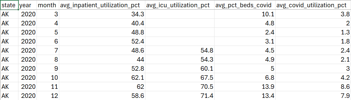
Syed Shameerur Rahman

Syed Shameerur Rahman

Syed is a Software Development Engineer at Amazon EMR. He is interested in highly scalable, distributed computing. He is an active contributor of open source projects like Apache Hive, Apache Tez, Apache ORC, and Apache Hadoop, and has contributed important features and optimizations. During his free time, he enjoys exploring new places and trying new foods.

Rajarshi Sarkar

Rajarshi Sarkar

Rajarshi is a Software Development Engineer at Amazon EMR. He works on cutting-edge features of Amazon EMR and is also involved in open source projects such as Apache Hive, Iceberg, Trino, and Hadoop. In his spare time, he likes to travel, watch movies, and hang out with friends.

Unlock the power of Apache Iceberg v3 deletion vectors on Amazon EMR

Post Syndicated from Arun Shanmugam original https://aws.amazon.com/blogs/big-data/unlock-the-power-of-apache-iceberg-v3-deletion-vectors-on-amazon-emr/

As modern data architectures expand, Apache Iceberg has become a widely popular open table format, providing ACID transactions, time travel, and schema evolution. In table format v2, Iceberg introduced merge-on-read, improving delete and update handling through positional delete files. These files improve write performance but can slow down reads when not compacted, since Iceberg must merge them during query execution to return the latest snapshot. Iceberg v3 enhances merge performance during reads by replacing positional delete files with deletion vectors for handling row-level deletes in Merge-on-Read (MoR) tables. This change deprecates the use of positional delete files in v3, which marked specific row positions as deleted, in favor of the more efficient deletion vectors.

In this post, we compare and evaluate the performance of the new binary deletion vectors in Iceberg v3 with respect to traditional position delete files of Iceberg v2 using Amazon EMR version 7.10.0 with Apache Spark 3.5.5. We provide insights into the practical impacts of these advanced row-level delete mechanisms on data management efficiency and performance.

Understanding binary deletion vectors and Puffin files

Binary deletion vectors stored in Puffin files use compressed bitmaps to efficiently represent which rows have been deleted within a data file. In contrast, previous Iceberg versions (v2) relied on positional delete files—Parquet files that enumerated rows to delete by file and position. This older approach resulted in many small delete files, which placed a heavy burden on query engines due to numerous file reads and costly in-memory conversions. Puffin files reduce this overhead by compactly encoding deletions, improving query performance and resource utilization.

Iceberg v3 improves this in the following aspects:

  • Reduced I/O – Fewer small delete files lower metadata overhead by introducing deletion vectors—compressed bitmaps that efficiently represent deleted rows. These vectors are stored persistently in Puffin files, a compact binary format optimized for low-latency access.
  • Query performance – Bitmap-based deletion vectors enable faster scan filtering by allowing multiple vectors to be stored in a single Puffin file. This reduces metadata and file count overhead while preserving file-level granularity for efficient reads. The design supports continuous merging of deletion vectors, promoting ongoing compaction that maintains stable query performance and reduces fragmentation over time. It removes the trade-off between partition-level and file-level delete granularity seen in v2, enabling consistently fast reads even in heavy-update scenarios.
  • Storage efficiency – Iceberg v3 uses a compressed binary format instead of verbose Parquet positioning. Engines maintain a single deletion vector per data file at write time, enabling better compaction and consistent query performance.

Solution overview

To explore the performance characteristics of delete operations in Iceberg v2 and v3, we use PySpark to run our comparison tests focusing on delete operation runtime and delete file size. This implementation helps us effectively benchmark and compare the deletion mechanisms between Iceberg v2’s position-delete files using Parquet and v3’s newer Puffin-based deletion vectors.

Our solution demonstrates how to configure Spark with the AWS Glue Data Catalog and Iceberg, create tables, and run delete operations programmatically. We first create Iceberg tables with format versions 2 and 3, insert 10,000 rows, then perform delete operations on a range of record IDs. We also perform table compaction and then measure delete operation runtime and size and count of associated delete files.

In Iceberg v3, deleting rows introduces binary deletion vectors stored in Puffin files (compact binary sidecar files). These allow more efficient query planning and faster read performance by consolidating deletes and avoiding large numbers of small files.

For this test, the Spark job was submitted by SSH’ing into the EMR cluster and using spark-submit directly from the shell, with the required Iceberg JAR file being referenced directly from the Amazon Simple Storage Service (Amazon S3) bucket in the submission command. When running the job, make sure you provide your S3 bucket name. See the following code:

spark-submit --jars s3://< S3-BUCKET-NAME >/iceberg/jars/iceberg-spark-runtime-3.5_2.12-1.9.2.jar v3_deletion_vector_test.py

Prerequisites

To follow along with this post, you must have the following prerequisites:

  • Amazon EMR on Amazon EC2 with version 7.10.0 integrated with the Glue Data Catalog, which includes Spark 3.5.5.
  • The Iceberg 1.9.2 JAR file from the official Iceberg documentation, which includes important deletion vector improvements such as v2 to v3 rewrites and dangling deletion vector detection. Optionally, you can use the default Iceberg 1.8.1-amzn-0 bundled with Amazon EMR 7.10 if these Iceberg 1.9.x improvements are not required.
  • An S3 bucket to store Iceberg data.
  • An AWS Identity and Access management (IAM) role for Amazon EMR configured with the necessary permissions.

The upcoming Amazon EMR 7.11 will ship with Iceberg 1.9.1-amzn-1, which includes deletion vector improvements such as v2 to v3 rewrites and dangling deletion vector detection. This means you no longer need to manually download or upload the Iceberg JAR file, because it will be included and managed natively by Amazon EMR.

Code walkthrough

The following PySpark script demonstrates how to create, write, compact, and delete records in Iceberg tables with two different format versions (v2 and v3) using the Glue Data Catalog as the metastore. The main goal is to compare both write and read performance, along with storage characteristics (delete file format and size) between Iceberg format versions 2 and 3.

The code performs the following functions:

  • Creates a SparkSession configured to use Iceberg with Glue Data Catalog integration.
  • Creates a synthetic dataset simulating user records:
    • Uses a fixed random seed (42) to provide consistent data generation
    • Creates identical datasets for both v2 and v3 tables for fair comparison
  • Defines the function test_read_performance(table_name) to perform the following actions:
    • Measure full table scan performance
    • Measure filtered read performance (with WHERE clause)
    • Track record counts for both operations
  • Defines the function test_iceberg_table(version, test_df) to perform the following actions:
    • Create or use an Iceberg table for the specified format version
    • Append data to the Iceberg table
    • Trigger Iceberg’s data compaction using a system procedure
    • Delete rows with IDs between 1000–1099
    • Collect statistics about inserted data files and delete-related files
    • Measure and record read performance metrics
    • Track operation timing for inserts, deletes, and reads
  • Defines a function to print a comprehensive comparative report including the following information:
    • Delete operation performance
    • Read performance (both full table and filtered)
    • Delete file characteristics (formats, counts, sizes)
    • Performance improvements as percentages
    • Storage efficiency metrics
  • Orchestrate the main execution flow:
    • Create a single dataset to ensure identical data for both versions
    • Clean up existing tables for fresh testing
    • Run tests for Iceberg format version 2 and version 3
    • Output a detailed comparison report
    • Handle exceptions and shut down the Spark session

See the following code:

from pyspark.sql import SparkSession
from pyspark.sql.types import StructType, StructField, IntegerType, StringType
from pyspark.sql import functions as F
import time
import random
import logging
from pyspark.sql.utils import AnalysisException
# Logging
logging.basicConfig(level=logging.INFO, format='%(message)s')
logger = logging.getLogger(__name__)
# Constants
ROWS_COUNT = 10000
DELETE_RANGE_START = 1000
DELETE_RANGE_END = 1099
SAMPLE_NAMES = ["Alice", "Bob", "Charlie", "Diana",
                "Eve", "Frank", "Grace", "Henry", "Ivy", "Jack"]
# Spark Session
spark = (
    SparkSession.builder
    .appName("IcebergWithGlueCatalog")
    .config("spark.sql.extensions", "org.apache.iceberg.spark.extensions.IcebergSparkSessionExtensions")
    .config("spark.sql.catalog.glue_catalog", "org.apache.iceberg.spark.SparkCatalog")
    .config("spark.sql.catalog.glue_catalog.catalog-impl", "org.apache.iceberg.aws.glue.GlueCatalog")
    .config("spark.sql.catalog.glue_catalog.warehouse", "s3://<S3-BUCKET-NAME>/blog/glue/")
    .config("spark.sql.catalog.glue_catalog.io-impl", "org.apache.iceberg.aws.s3.S3FileIO")
    .getOrCreate()
)
spark.sql("CREATE DATABASE IF NOT EXISTS glue_catalog.blog")
def create_dataset(num_rows=ROWS_COUNT):
    # Set a fixed seed for reproducibility
    random.seed(42)
    
    data = [(i,
             random.choice(SAMPLE_NAMES) + str(i),
             random.randint(18, 80))
            for i in range(1, num_rows + 1)]
    schema = StructType([
        StructField("id", IntegerType(), False),
        StructField("name", StringType(), True),
        StructField("age", IntegerType(), True)
    ])
    df = spark.createDataFrame(data, schema)
    df = df.withColumn("created_at", F.current_timestamp())
    return df
def test_read_performance(table_name):
    """Test read performance of the table"""
    start_time = time.time()
    count = spark.sql(f"SELECT COUNT(*) FROM glue_catalog.blog.{table_name}").collect()[0][0]
    read_time = time.time() - start_time
    
    # Test filtered read performance
    start_time = time.time()
    filtered_count = spark.sql(f"""
        SELECT COUNT(*) 
        FROM glue_catalog.blog.{table_name} 
        WHERE age > 30
    """).collect()[0][0]
    filtered_read_time = time.time() - start_time
    
    return read_time, filtered_read_time, count, filtered_count
def test_iceberg_table(version, test_df):
    try:
        table_name = f"iceberg_table_v{version}"
        logger.info(f"\n=== TESTING ICEBERG V{version} ===")
        spark.sql(f"""
            CREATE TABLE IF NOT EXISTS glue_catalog.blog.{table_name} (
                id int,
                name string,
                age int,
                created_at timestamp
            ) USING iceberg
            TBLPROPERTIES (
                'format-version'='{version}',
                'write.delete.mode'='merge-on-read'
            )
        """)
        start_time = time.time()
        test_df.writeTo(f"glue_catalog.blog.{table_name}").append()
        insert_time = time.time() - start_time
        logger.info("Compaction...")
        spark.sql(
            f"CALL glue_catalog.system.rewrite_data_files('glue_catalog.blog.{table_name}')")
        start_time = time.time()
        spark.sql(f"""
            DELETE FROM glue_catalog.blog.{table_name}
            WHERE id BETWEEN {DELETE_RANGE_START} AND {DELETE_RANGE_END}
        """)
        delete_time = time.time() - start_time
        files_df = spark.sql(
            f"SELECT COUNT(*) as data_files FROM glue_catalog.blog.{table_name}.files")
        delete_files_df = spark.sql(f"""
            SELECT COUNT(*) as delete_files,
                   file_format,
                   SUM(file_size_in_bytes) as total_size
            FROM glue_catalog.blog.{table_name}.delete_files
            GROUP BY file_format
        """)
        data_files = files_df.collect()[0]['data_files']
        delete_stats = delete_files_df.collect()
        # Add read performance testing
        logger.info("\nTesting read performance...")
        read_time, filtered_read_time, total_count, filtered_count = test_read_performance(table_name)
        
        logger.info(f"Insert time: {insert_time:.3f}s")
        logger.info(f"Delete time: {delete_time:.3f}s")
        logger.info(f"Full table read time: {read_time:.3f}s")
        logger.info(f"Filtered read time: {filtered_read_time:.3f}s")
        logger.info(f"Data files: {data_files}")
        logger.info(f"Total records: {total_count}")
        logger.info(f"Filtered records: {filtered_count}")
        if len(delete_stats) > 0:
            stats = delete_stats[0]
            logger.info(f"Delete files: {stats.delete_files}")
            logger.info(f"Delete format: {stats.file_format}")
            logger.info(f"Delete files size: {stats.total_size} bytes")
            return delete_time, stats.total_size, stats.file_format, read_time, filtered_read_time
        else:
            logger.info("No delete files found")
            return delete_time, 0, "N/A", read_time, filtered_read_time
    except AnalysisException as e:
        logger.error(f"SQL Error: {str(e)}")
        raise
    except Exception as e:
        logger.error(f"Error: {str(e)}")
        raise
def print_comparison_results(v2_results, v3_results):
    v2_delete_time, v2_size, v2_format, v2_read_time, v2_filtered_read_time = v2_results
    v3_delete_time, v3_size, v3_format, v3_read_time, v3_filtered_read_time = v3_results
    logger.info("\n=== PERFORMANCE COMPARISON ===")
    logger.info(f"v2 delete time: {v2_delete_time:.3f}s")
    logger.info(f"v3 delete time: {v3_delete_time:.3f}s")
    if v2_delete_time > 0:
        improvement = ((v2_delete_time - v3_delete_time) / v2_delete_time) * 100
        logger.info(f"v3 Delete performance improvement: {improvement:.1f}%")
    logger.info("\n=== READ PERFORMANCE COMPARISON ===")
    logger.info(f"v2 full table read time: {v2_read_time:.3f}s")
    logger.info(f"v3 full table read time: {v3_read_time:.3f}s")
    logger.info(f"v2 filtered read time: {v2_filtered_read_time:.3f}s")
    logger.info(f"v3 filtered read time: {v3_filtered_read_time:.3f}s")
    
    if v2_read_time > 0:
        read_improvement = ((v2_read_time - v3_read_time) / v2_read_time) * 100
        logger.info(f"v3 Read performance improvement: {read_improvement:.1f}%")
    
    if v2_filtered_read_time > 0:
        filtered_improvement = ((v2_filtered_read_time - v3_filtered_read_time) / v2_filtered_read_time) * 100
        logger.info(f"v3 Filtered read performance improvement: {filtered_improvement:.1f}%")
    logger.info("\n=== DELETE FILE COMPARISON ===")
    logger.info(f"v2 delete format: {v2_format}")
    logger.info(f"v2 delete size: {v2_size} bytes")
    logger.info(f"v3 delete format: {v3_format}")
    logger.info(f"v3 delete size: {v3_size} bytes")
    if v2_size > 0:
        size_reduction = ((v2_size - v3_size) / v2_size) * 100
        logger.info(f"v3 size reduction: {size_reduction:.1f}%")
# Main
try:
    # Create dataset once and reuse for both versions
    test_dataset = create_dataset()
    
    # Drop existing tables if they exist
    spark.sql("DROP TABLE IF EXISTS glue_catalog.blog.iceberg_table_v2")
    spark.sql("DROP TABLE IF EXISTS glue_catalog.blog.iceberg_table_v3")
    
    # Test both versions with the same dataset
    v2_results = test_iceberg_table(2, test_dataset)
    v3_results = test_iceberg_table(3, test_dataset)
    print_comparison_results(v2_results, v3_results)
finally:
    spark.stop()

Results summary

The output generated by the code includes the results summary section that shows several key comparisons, as shown in the following screenshot. For delete operations, Iceberg v3 uses the Puffin file format compared to Parquet in v2, resulting in significant improvements. The delete operation time decreased from 3.126 seconds in v2 to 1.407 seconds in v3, achieving a 55.0% performance improvement. Additionally, the delete file size was reduced from 1801 bytes using Parquet in v2 to 475 bytes using Puffin in v3, representing a 73.6% reduction in storage overhead. Read operations also saw notable improvements, with full table reads 28.5% faster and filtered reads 23% faster in v3. These improvements demonstrate the efficiency gains from v3’s implementation of binary deletion vectors through the Puffin format.

style=

The actual measured performance and storage improvements depend on workload and environment and might differ from the preceding example.

This following screenshot from the S3 bucket demonstrates a Puffin delete file stored alongside data files.

style=

Clean up

After you finish your tests, it’s important to clean up your environment to avoid unnecessary costs:

  1. Drop the test tables you created to remove associated data from your S3 bucket and prevent ongoing storage charges.
  2. Delete any temporary data left in the S3 bucket used for Iceberg data.
  3. Delete the EMR cluster to stop billing for running compute resources.

Cleaning up resources promptly helps maintain cost-efficiency and resource hygiene in your AWS environment.

Considerations

Iceberg features are introduced through a phased process: first in the specification, then in the core library, and finally in engine implementations. Deletion vector support is currently available in the specification and core library, with Spark being the only supported engine. We validated this capability on Amazon EMR 7.10 with Spark 3.5.5.

Conclusion

Iceberg v3 introduces a significant advancement in managing row-level deletes for merge-on-read operations through binary deletion vectors stored in compact Puffin files. Our performance tests, conducted with Iceberg 1.9.2 on Amazon EMR 7.10.0 and EMR Spark 3.5.5, show clear improvements in both delete operation speed and read performance, along with a considerable reduction in delete file storage compared to Iceberg v2’s positional delete Parquet files. For more information about deletion vectors, refer to Iceberg v3 deletion vectors.


About the authors

Arun Shanmugam

Arun Shanmugam

Arun is a Senior Analytics Solutions Architect at AWS, with a focus on building modern data architecture. He has been successfully delivering scalable data analytics solutions for customers across diverse industries. Outside of work, Arun is an avid outdoor enthusiast who actively engages in CrossFit, road biking, and cricket.

Suthan Phillips

Suthan Phillips

Suthan is a Senior Analytics Architect at AWS, where he helps customers design and optimize scalable, high-performance data solutions that drive business insights. He combines architectural guidance on system design and scalability with best practices to provide efficient, secure implementation across data processing and experience layers. Outside of work, Suthan enjoys swimming, hiking, and exploring the Pacific Northwest.

Kinshuk Paharae

Kinshuk Paharae

Kinshuk is head of product for data processing, leading product teams for AWS Glue, Amazon EMR, and Amazon Athena. He has been with AWS for over 5 years.

Linda OConnor

Linda OConnor

Linda is a Seasoned Go-To-Market Leader with close to three decades of experience driving growth strategies in the data and analytics space. At AWS, she currently leads pan analytics initiatives including lakehouse architectures, helping customers transform their existing landscapes through non-disruptive innovation. She previously served as Global Vice President at a German software company for 25 years, where she spearheaded Data Warehousing and Big Data portfolios, orchestrating successful product launches and driving global market expansion.

Automate and orchestrate Amazon EMR jobs using AWS Step Functions and Amazon EventBridge

Post Syndicated from Senthil Kamala Rathinam original https://aws.amazon.com/blogs/big-data/automate-and-orchestrate-amazon-emr-jobs-using-aws-step-functions-and-amazon-eventbridge/

Many enterprises are adopting Apache Spark for scalable data processing tasks such as extract, transform, and load (ETL), batch analytics, and data enrichment. As data pipelines evolve, the need for flexible and cost-efficient execution environments that support automation, governance, and performance at scale also evolve in parallel. Amazon EMR provides a powerful environment to run Spark workloads, and depending on workload characteristics and compliance requirements, teams can choose between fully managed options like Amazon EMR Serverless or more customizable configurations using Amazon EMR on Amazon Elastic Compute Cloud (Amazon EC2).

In use cases where infrastructure control, data locality, or strict security postures are essential, such as in financial services, healthcare, or government, running transient EMR on EC2 clusters becomes a preferred choice. However, orchestrating the full lifecycle of these clusters, from provisioning to job submission and eventual teardown, can introduce operational overhead and risk if done manually.

To streamline this process, the AWS Cloud offers built-in orchestration capabilities using AWS Step Functions and Amazon EventBridge. Together, these services help you automate and schedule the entire EMR job lifecycle, reducing manual intervention while optimizing cost and compliance. Step Functions provides the workflow logic to manage cluster creation, Spark job execution, and cluster termination, and EventBridge schedules these workflows based on business or operational needs.

In this post, we discuss how to build a fully automated, scheduled Spark processing pipeline using Amazon EMR on EC2, orchestrated with Step Functions and triggered by EventBridge. We walk through how to deploy this solution using AWS CloudFormation, processes COVID-19 public dataset data in Amazon Simple Storage Service (Amazon S3), and store the aggregated results in Amazon S3. This architecture is ideal for periodic or scheduled batch processing scenarios where infrastructure control, auditability, and cost-efficiency are critical.

Solution overview

This solution uses the publicly available COVID-19 dataset to illustrate how to build a modular, scheduled architecture for scalable and cost-efficient batch processing for time-bound data workloads.The solution follows these steps:

  1. Raw COVID-19 data in CSV format is stored in an S3 input bucket.
  2. A scheduled rule in EventBridge triggers a Step Functions workflow.
  3. The Step Functions workflow provisions a transient Amazon EMR cluster using EC2 instances.
  4. A PySpark job is submitted to the cluster to calculate COVID-19 hospital utilization data to compute monthly state-level averages of inpatient and ICU bed utilization, and COVID-19 patient percentages.
  5. The processed results are written back to an S3 output bucket.
  6. After successful job completion, the EMR cluster is automatically deleted.
  7. Logs are persisted to Amazon S3 for observability and troubleshooting.

By automating this workflow, you alleviate the need to manually manage EMR clusters while gaining cost-efficiency by running compute only when needed. This architecture is ideal for periodic Spark jobs such as ETL pipelines, regulatory reporting, and batch analytics, especially when control, compliance, and customization are required.The following diagram illustrates the architecture for this use case.

The infrastructure is deployed using AWS CloudFormation to provide consistency and repeatability. AWS Identity and Access Management (IAM) roles grant least‑privilege access to Step Functions, Amazon EMR, EC2 instances, and S3 buckets, and optional AWS Key Management Service (AWS KMS) encryption can secure data at rest in Amazon S3 and Amazon CloudWatch Logs. By combining a scheduled trigger, stateful orchestration, and centralized logging, this solution delivers a fully automated, cost‑optimized, and secure way to run transient Spark workloads in production.

Prerequisites

Before you get started, make sure you have the following prerequisites:

Set up resources with AWS CloudFormation

To provision the required resources using a single CloudFormation template, complete the following steps:

  1. Sign in to the AWS Management Console as an admin user.
  2. Clone the sample repository to your local machine or AWS CloudShell and navigate into the project directory.
    git clone https://github.com/aws-samples/sample-emr-transient-cluster-step-functions-eventbridge.git
    cd sample-emr-transient-cluster-step-functions-eventbridge

  3. Set an environment variable for the AWS Region where you plan to deploy the resources. Replace the placeholder with your Region code, for example, us-east-1.
    export AWS_REGION=<YOUR AWS REGION>

  4. Deploy the stack using the following command. Update the stack name if needed. In this example, the stack is created with the name covid19-analysis.
    aws cloudformation deploy \
    --template-file emr_transient_cluster_step_functions_eventbridge.yaml \
    --stack-name covid19-analysis \
    --capabilities CAPABILITY_IAM \
    --region $AWS_REGION 

You can monitor the stack creation progress on the AWS CloudFormation console on the Events tab. The deployment typically completes in under 5 minutes.

After the stack is successfully created, go to the Outputs tab on the AWS CloudFormation console and note the following values for use in later steps:

  • InputBucketName
  • OutputBucketName
  • LogBucketName

Set up the COVID-19 dataset

With your infrastructure in place, complete the following steps to set up the input data:

  1. Download the COVID-19 data CSV file from HealthData.gov to your local machine.
  2. Rename the downloaded file to covid19-dataset.csv.
  3. Upload the renamed file to your S3 input bucket under the raw/ folder path.

Set up the PySpark Script

Complete the following steps to set up the PySpark script:

  1. Open AWS CloudShell from the console.
  2. Confirm that you are working inside the sample-emr-transient-cluster-step-functions-eventbridge directory before running the next command.
  3. Copy the PySpark script needed for this walkthrough into your input bucket:
    aws s3 cp covid19_processor.py s3://<InputBucketName>/scripts/

This script processes COVID-19 hospital utilization data stored as CSV files in your S3 input bucket. When running the job, provide the following command-line arguments:

  • --input – The S3 path to the input CSV files
  • --output – The S3 path to store the processed results

The script reads the raw dataset, standardizes various date formats, and filters out records with invalid or missing dates. It then extracts key utilization metrics such as inpatient bed usage, ICU bed usage, and the percentage of beds occupied by COVID-19 patients and calculates monthly averages grouped by state. The aggregated output is saved as timestamped CSV files in the specified S3 location.

This example demonstrates how you can use PySpark to efficiently clean, transform, and analyze large-scale healthcare data to gain actionable insights on hospital capacity trends during the pandemic.

Configure a schedule in EventBridge

The Step Functions state machine is by default scheduled to run on December 31, 2025, as a one-time execution. You can update the schedule for recurring or one-time execution as needed. Complete the following steps:

  1. On the EventBridge console, choose Schedules under Scheduler in the navigation pane.
  2. Select the schedule named <StackName>-covid19-analysis and choose Edit.
  3. Set your preferred schedule pattern.
    1. If you want to run the schedule one time, select One-time schedule for Occurrence and enter a date and time.
    2. If you want to run this on a recurring basis, select Recurring schedule. Specify the schedule type as either Cron-based schedule or Rate-based schedule as needed.
  4. Choose Next twice and choose Save schedule.

Start the workflow in Step Functions

Based on your EventBridge schedule, the Step Functions workflow will run automatically. For this walkthrough, complete the following steps to trigger it manually:

  1. On the Step Functions console, choose State machines in the navigation pane.
  2. Choose the state machine that begins with Covid19AnalysisStateMachine-*.
  3. Choose Start execution.
  4. In the Input section, provide the following JSON (provide the log bucket and output bucket names with the appropriate values captured earlier):
    {
      "LogUri": "s3://<LogBucketName>/logs/",
      "OutputS3Location": "s3://<OutputBucketName>/processed/"
    }

  5. Choose Start execution to initiate the workflow.

Monitor the EMR job and workflow execution

After you start the workflow, you can track both the Step Functions state transitions and the EMR job progress in real time on the console.

Monitor the Step Functions state machine

Complete the following steps to monitor the Step Functions state machine:

  1. On the Step Functions console, choose State machines in the navigation pane.
  2. Choose the state machine that begins with Covid19AnalysisStateMachine-*.
  3. Choose the running execution to view the visual workflow.

    Each state node will update as it progresses—green for success, red for failure.

  4. To explore a step, choose its node and inspect the input, output, and error details in the side pane.

The following screenshot shows an example of a successfully executed workflow.

Monitor the EMR cluster and EMR step

Complete the following steps to monitor the EMR cluster and EMR step status:

  1. While the cluster is active, open the Amazon EMR console and choose Clusters in the navigation pane.
  2. Locate the Covid19Cluster transient EMR cluster.
    Initially, it will be in Starting status.

    On the Steps tab, you can see your Spark submit step listed. As the job progresses, the step status changes from Pending to Running to finally Completed or Failed.

  3. Choose the Applications tab to view the application UIs, in which you can access the Spark History Server and YARN Timeline Server for monitoring and troubleshooting.

Monitor CloudWatch logs

To enable CloudWatch logging and enhanced monitoring for your EMR on EC2 cluster, refer to Amazon EMR on EC2 – Enhanced Monitoring with CloudWatch using custom metrics and logs. This guide explains how to install and configure the CloudWatch agent using a bootstrap action, so you can stream system-level metrics (such as CPU, memory, and disk usage) and application logs from EMR nodes directly to CloudWatch. With this setup, you can gain real-time visibility into cluster health and performance, simplify troubleshooting, and retain critical logs even after the cluster is terminated.

For this walkthrough, check the logs in the S3 log output location.

Confirm cluster deletion

When the Spark step is complete, Step Functions will automatically delete the Amazon EMR cluster. Refresh the Clusters page on the Amazon EMR console. You should see your cluster status change from Terminating to Terminated within a minute.

By following these steps, you gain full end-to-end visibility into your workflow from the moment the Step Functions state machine is triggered to the automatic shutdown of the EMR cluster. You can monitor execution progress, troubleshoot issues, confirm job success, and continuously optimize your transient Spark workloads.

Verify job output in Amazon S3

When the job is complete, complete the following steps to check the processed results in the S3 output bucket:

  1. On the Amazon S3 console, choose Buckets in the navigation pane.
  2. Open the output S3 bucket you noted earlier.
  3. Open the processed folder.
  4. Navigate into the timestamped subfolder to view the CSV output file.
  5. Download the CSV file to view the processed results, as shown in the following screenshot.

Monitoring and troubleshooting

To monitor the progress of your Spark job running on a transient EMR on EC2 cluster, use the Step Functions console. It provides real-time visibility into each state transition in your workflow, from cluster creation and job submission to cluster deletion. This makes it straightforward to track execution flow and identify where issues might occur.During job execution, you can use the Amazon EMR console to access cluster-level monitoring. This includes YARN application statuses, step-level logs, and overall cluster health. If CloudWatch logging is enabled in your job configuration, driver and executor logs stream in near real time, so you can quickly detect and diagnose errors, resource constraints, or data skew within your Spark application.

After the workflow is complete, regardless of whether it succeeds or fails, you can perform a detailed post-execution analysis by reviewing the logs stored in the S3 bucket specified in the LogUri parameter. This log directory includes standard output and error logs, along with Spark history files, offering insights into execution behavior and performance metrics.

For continued access to the Spark UI during job execution, you can use persistent application UIs on the EMR console. These links remain accessible even after the cluster is stopped, enabling deeper root-cause analysis and performance tuning for future runs.

This visibility into both workflow orchestration and job execution can help teams optimize their Spark workloads, reduce troubleshooting time, and build confidence in their EMR automation pipelines.

Clean up

To avoid incurring ongoing charges, clean up the resources provisioned during this walkthrough:

  1. Empty the S3 buckets:
    1. On the Amazon S3 console, choose Buckets in the navigation pane.
    2. Select the input, output, and log buckets used in this tutorial.
    3. Choose Empty to remove all objects before deleting the buckets (optional).
  2. Delete the CloudFormation stack:
    1. On the AWS CloudFormation console, choose Stacks in the navigation pane.
    2. Select the stack you created for this solution and choose Delete.
    3. Confirm the deletion to remove associated resources.

Conclusion

In this post, we showed how to build a fully automated and cost-effective Spark processing pipeline using Step Functions, EventBridge, and Amazon EMR on EC2. The workflow provisions a transient EMR cluster, runs a Spark job to process data, and stops the cluster after the job completes. This approach helps reduce costs while giving you full control over the process. This solution is ideal for scheduled data processing tasks such as ETL jobs, log analytics, or batch reporting, especially when you need detailed control over infrastructure, security, and compliance settings.

To get started, deploy the solution in your environment using the CloudFormation stack provided and adjust it to fit your data processing needs. Check out the Step Functions Developer Guide and Amazon EMR Management Guide to explore further.

Share your feedback and ideas in the comments or connect with your AWS Solutions Architect to fine-tune this pattern for your use case.


About the authors

Senthil Kamala Rathinam

Senthil Kamala Rathinam

Senthil is a Solutions Architect at Amazon Web Services, specializing in Data and Analytics for banking customers across North America. With deep expertise in Data and Analytics, AI/ML, and Generative AI, he helps organizations unlock business value through data-driven transformation. Beyond work, Senthil enjoys spending time with his family and playing badminton.

Shashi Makkapati

Shashi Makkapati

Shashi is a Senior Solutions Architect serving banking customers across North America. He specializes in data analytics, AI/ML, and generative AI, focusing on innovative solutions that transform financial organizations. Shashi is passionate about leveraging technology to solve complex business challenges in the banking sector. Outside of work, he enjoys traveling and spending quality time with his family.

Streamline Spark application development on Amazon EMR with the Data Solutions Framework on AWS

Post Syndicated from Vincent Gromakowski original https://aws.amazon.com/blogs/big-data/streamline-spark-application-development-on-amazon-emr-with-the-data-solutions-framework-on-aws/

Today, organizations are heavily using Apache Spark for their big data processing needs. However, managing the entire development lifecycle of Spark applications—from local development to production deployment—can be complex and time-consuming. Managing the entire code base—including application code, infrastructure provisioning, and continuous integration and delivery (CI/CD) pipelines—is sometimes not fully automated and a shared responsibility across multiple teams, which slows down release cycles. This undifferentiated heavy lifting diverts valuable resources away from core business objectives: deriving value from data.

In this post, we explore how to use Amazon EMR, the AWS Cloud Development Kit (AWS CDK), and the Data Solutions Framework (DSF) on AWS to streamline the development process, from setting up a local development environment to deploying serverless Spark infrastructure, and implementing a CI/CD pipeline for automated testing and deployment.

By adopting this approach, developers gain full control over their code and the infrastructure responsible for running it, alleviating the need for cross-team dependency. Developers can customize the infrastructure to meet specific business needs and optimize performance. Additionally, they can customize CI/CD stages to facilitate comprehensive testing, using the self-mutation capability of AWS CDK Pipelines to automatically update and refine the deployment process. This level of control not only accelerates development cycles but also enhances the reliability and efficiency of the entire application lifecycle, so developers can focus more on innovation and less on manual infrastructure management.

Solution overview

The solution consists of the following key components:

  • The local development environment to develop and test your Spark code locally
  • The infrastructure as code (IaC) that will run your Spark application in AWS environments
  • The CI/CD pipeline running end-to-end tests and deploying into the different AWS environments

In the following sections, we discuss how to set up these components.

Prerequisites

To set up this solution, you must have an AWS account with appropriate permissions, Docker and the AWS CDK CLI.

Set up the local development environment

Developing Spark applications locally can be a challenging task due to the need for a consistent and efficient environment that mirrors your production setup. With Amazon EMR, Docker, and the Amazon EMR toolkit extension for Visual Studio Code, you can quickly set up a local development environment for Spark applications, developing and testing Spark code locally, and seamlessly port it to the cloud.

The Amazon EMR toolkit for VS Code includes an “EMR: Create Local Spark Environment” command that generates a development container. This container is based on an Amazon EMR on Amazon EKS image corresponding to the Amazon EMR version you select. You can develop Spark and PySpark code locally, with full compatibility with your remote Amazon EMR environment. Additionally, the toolkit provides helpers to make it straightforward to connect to the AWS Cloud, including an Amazon EMR explorer, an AWS Glue Data Catalog explorer, and commands to run Amazon EMR Serverless jobs from VS Code.

To set up your local environment, complete the following steps:

  1. Install VS Code and the Amazon EMR Toolkit for VS Code.
  2. Install and launch Docker.
  3. Create a local Amazon EMR environment in your working directory using the command EMR: Create Local Spark Environment.

Amazon EMR Toolkit bootstrap

  1. Choose PySpark, Amazon EMR 7.5, and the AWS Region you want to use, and choose an authentication mechanism.

Amazon EMR toolkit local environment

  1. Log in to Amazon ECR with your AWS credentials using the following command so you can download the Amazon EMR image:
aws ecr get-login-password --region us-east-1 \
    | docker login \
    --username AWS \
    --password-stdin \
    12345678910.dkr.ecr.us-east-1.amazonaws.com
  1. Now you can launch your dev container using the VS Code command Dev Containers: Rebuild and Reopen in container.

The container will install the latest operating system packages and run a local Spark history server on port 18080.

local Spark history server

The container provides spark-shell, spark-sql, and pyspark from the terminal and a Jupyter Python kernel for connecting a Jupyter notebook to execute interactive Spark code.

local Jupyter notebooks

Using the Amazon EMR Toolkit, you can develop your Spark application and test it locally using Pytest—for example, to validate the business logic. You can also connect to other AWS accounts where you have your development environment.

Build the AWS CDK application with DSF on AWS

After you validate the business logic into your local Spark application, you can implement the infrastructure responsible for running your application. DSF provides AWS CDK L3 Constructs that simplify the creation of Spark-based data pipelines on EMR Serverless or Amazon EMR on EKS.

DSF provides the capability to package your local PySpark application, including the Python dependencies, into artifacts that can consumed by EMR Serverless jobs. The PySparkApplicationPackage is a construct that uses a Dockerfile to perform the packaging of dependencies into a Python virtual environment archive and then upload the archive and the PySpark entrypoint file into a secured Amazon Simple Storage Service (Amazon S3) bucket. The following diagram illustrates this architecture.

PySparkApplicationPackage L3 construct

See the following example code:

spark_app = dsf.processing.PySparkApplicationPackage(
    self,
    "SparkApp",
    entrypoint_path="./../spark/src/agg_trip_distance.py",
    application_name="TaxiAggregation",
    # Path of the Dockerfile used to package the dependencies as a Python venv
    dependencies_folder='./../spark',
    # Path of the venv archive in the docker image
    venv_archive_path="/venv-package/pyspark-env.tar.gz",
    removal_policy=RemovalPolicy.DESTROY)

You just need to provide the paths for the following:

  • The PySpark entrypoint. This is the main Python script of your Spark application.
  • The Dockerfile containing the logic for packaging a virtual environment into an archive.
  • The path of the resulting archive in the container file system.

DSF provides helpers to connect the application package to the EMR Serverless job. The PySparkApplicationPackage construct exposes properties that can directly be used into the SparkEmrServerlessJob construct parameters. This construct simplifies the configuration of a batch job using an AWS Step Functions state machine. The following diagram illustrates this architecture.

EmrServerlessJob L3 construct

The following code is an example of an EMR Serverless job:

spark_job = dsf.processing.SparkEmrServerlessJob(
    self,
    "SparkProcessingJob",
    dsf.processing.SparkEmrServerlessJobProps(
        name=f"taxi-agg-job-{Names.unique_resource_name(self)}",
        # ID of the previously created EMR Serverless runtime
        application_id=spark_runtime.application.attr_application_id,
        # The IAM role used by the EMR Job with permissions required by the application
        execution_role=processing_exec_role,
        spark_submit_entry_point=spark_app.entrypoint_uri,
        # Add the Spark parameters from the PySpark package to configure the dependencies (using venv)
        spark_submit_parameters=spark_app.spark_venv_conf + spark_params,
        removal_policy=RemovalPolicy.DESTROY,
        schedule=schedule))

Note the two parameters of SparkEmrServerlessJob that are provided by PySparkApplicationPackage:

  • entrypoint_uri, which is the S3 URI of the entrypoint file
  • spark_venv_conf, which contains the Spark submit parameters for using the Python virtual environment

DSF also provides a SparkEmrServerlessRuntime to simplify the creation of the EMR Serverless application responsible for running the job.

Deploy the Spark application using CI/CD

The final step is to implement a CI/CD pipeline that can test your Spark code and promote from dev/test/stage and then to production. DSF provides a L3 Construct that simplifies the creation of the CI/CD pipeline for your Spark applications. DSF’s implementation of the Spark CI/CD pipeline construct uses the AWS CDK built-in pipeline functionality. One of the key capabilities when using an AWS CDK pipeline is its self-mutating capability. It can update itself whenever you change its definition, avoiding the traditional chicken-and-egg problem of pipeline updates and helping developers fully control their CI/CD pipeline.

When the pipeline runs, it follows a carefully orchestrated sequence. First, it retrieves your code from your repository and synthesizes it into AWS CloudFormation templates. Before doing anything else, it examines these templates to see if you’ve made any changes to the pipeline’s own structure. If the pipeline detects that its definition has changed, it will pause its normal operation and update itself first. After the pipeline has updated itself, it will continue with its regular stages, such as deploying your application.

DSF provides an opinionated implementation of CDK Pipelines for Spark applications, where the PySpark code is automatically unit tested using Pytest and where the configuration is simplified. You only need to configure four components:

  • The CI/CD stages (testing, staging, production, and so on). This includes the AWS account ID and Region where these environments reside in.
  • The AWS CDK stack that is deployed in each environment.
  • (Optional) The integration test script that you want to run against the deployed stack.
  • The SparkEmrCICDPipeline AWS CDK construct.

The following diagram illustrates how everything works together.

SparkCICDPipeline L3 construct

Let’s dive into each of these components.

Define cross-account deployment and CI/CD stages

With the SparkEmrCICDPipeline construct, you can deploy your Spark application stack across different AWS accounts. For example, you can have a separate account for your CI/CD processes and different accounts for your staging and production environments.To set this up, first bootstrap the various AWS accounts (staging, production, and so on):

cdk bootstrap --profile <ENVIRONMENT_ACCOUNT_PROFILE> \ 
    aws://<ENVIRONMENT_ACCOUNT_ID&gt;/&lt;REGION> \ 
    --trust <CICD_ACCOUNT_ID> \ 
    --cloudformation-execution-policies "POLICY_ARN"

This step sets up the necessary resources in the environment accounts and creates a trust relationship between those accounts and the CI/CD account where the pipeline will run.Next, choose between two options to define the environments (both options require the relevant configuration in the cdk.context.json file.The first option is to use pre-defined environments, which is defined as follows:

{ 
    "staging": { 
        "account": "<STAGING_ACCOUNT_ID>", 
        "region": "<REGION>" 
    }, 
    "prod": { 
        "account": "<PROD_ACCOUNT_ID>", 
        "region": "<REGION>" 
    } 
}

Alternatively, you can use user-defined environments, which is defined as follows:

{
   "environments":[
      {
         "stageName":"<STAGE_NAME_1>",
         "account":"<STAGE_ACCOUNT_ID>",
         "region":"<REGION>",
         "triggerIntegTest":"<OPTIONAL_BOOLEAN_CAN_BE_OMMITTED>"
      },
      {
         "stageName":"<STAGE_NAME_2>",
         "account":"<STAGE_ACCOUNT_ID>",
         "region":"<REGION>",
         "triggerIntegTest":"<OPTIONAL_BOOLEAN_CAN_BE_OMMITTED>"
      },
      {
         "stageName":"<STAGE_NAME_3>",
         "account":"<STAGE_ACCOUNT_ID>",
         "region":"<REGION>",
         "triggerIntegTest":"<OPTIONAL_BOOLEAN_CAN_BE_OMMITTED>"
      }
   ]
}

Customize the stack to be deployed

Now that the environments have been bootstrapped and configured, let’s look at the actual stack that contains the resources that will be deployed in the various environments. Two classes must be implemented:

  • A class that extends the stack – This is where the resources that are going to be deployed in each of the environments are defined. This can be a normal AWS CDK stack, but it can be deployed in another AWS account depending on the environment configuration defined in the previous section.
  • A class that extends ApplicationStackFactory – This is DSF specific, and makes it possible to configure and then return the stack that is created.

The following code shows a full example:

class MyApplicationStack(cdk.Stack): 
    def __init__(self, scope, *, stage): 
        super().__init__(scope, "MyApplicationStack") 
        bucket = Bucket(self, "TestBucket",
                        auto_delete_objects=True, 
                        removal_policy=cdk.RemovalPolicy.DESTROY) 
        cdk.CfnOutput(self, "BucketName", value=bucket.bucket_name) 
        
class MyStackFactory(dsf.utils.ApplicationStackFactory): 
    def create_stack(self, scope, stage): 
        return MyApplicationStack(scope, stage=stage)

ApplicationStackFactory supports customization of the stack before returning the initialized object to be deployed by the CI/CD pipeline. You can customize your stack behavior by passing the current stage to your stack. For example, you can skip scheduling the Spark application in the integration tests stage because the integration tests trigger it manually as part of the CI/CD pipeline. For the production stage, the scheduling facilitates automatic execution of the Spark application.

Write the integration test script

The integration test script is a bash script that is triggered after the main application stack has been deployed. Inputs to the bash script can come from the AWS CloudFormation outputs of the main application stack. These outputs are mapped into environment variables that the bash script can access directly.

In the Spark CI/CD example, the application stack uses the SparkEMRServerlessJob CDK construct. This construct uses a Step Functions state machine to manage the execution and monitoring of the Spark job. The following is an example integration test bash script that we use to test that the deployed stack can run the associated Spark job successfully:

#!/bin/bash 
EXECUTION_ARN=$(aws stepfunctions start-execution --state-machine-arn $STEP_FUNCTION_ARN | jq -r '.executionArn')

while true 
do 
    STATUS=$(aws stepfunctions describe-execution --execution-arn $EXECUTION_ARN | jq -r '.status') 
    if [ $STATUS = "SUCCEEDED" ]; then 
        exit 0 
    elif [ $STATUS = "FAILED" ] || [ $STATUS = "TIMED_OUT" ] || [ $STATUS = "ABORTED" ]; then 
        exit 1 
    else 
        sleep 10
        continue 
    fi
done

The integration test scripts are executed within an AWS CodeBuild project. As part of the IntegrationTestStack, we’ve included a custom resource that periodically checks the status of the integration test script as it runs. Failure of the CodeBuild execution causes the parent pipeline (residing in the pipeline account) to fail. This helps teams only promote changes that pass all the required testing.

Bring all the components together

When you have your components ready, you can use the SparkEmrCICDPipeline to bring them together. See the following example code:

dsf.processing.SparkEmrCICDPipeline(
    self,
    "SparkCICDPipeline",
    spark_application_name="SparkTest",
    # The Spark image to use in the CICD unit tests
    spark_image=dsf.processing.SparkImage.EMR_7_5,
    # The factory class to dynamically pass the Application Stack
    application_stack_factory=SparkApplicationStackFactory(),
    # Path of the CDK python application to be used by the CICD build and deploy phases
    cdk_application_path="infra",
    # Path of the Spark application to be built and unit tested in the CICD
    spark_application_path="spark",
    # Path of the bash script responsible to run integration tests 
    integ_test_script='./infra/resources/integ-test.sh',
    # Environment variables used by the integration test script, value is the CFN output name
    integ_test_env={
        "STEP_FUNCTION_ARN": "ProcessingStateMachineArn"
    },
    # Additional permissions to give to the CICD to run the integration tests
    integ_test_permissions=[
        PolicyStatement(
            actions=["states:StartExecution", "states:DescribeExecution"
            ],
            resources=["*"]
        )
    ],
    source= CodePipelineSource.connection("your/repo", "branch",
        connection_arn="arn:aws:codeconnections:us-east-1:222222222222:connection/7d2469ff-514a-4e4f-9003-5ca4a43cdc41"
    ),
    removal_policy=RemovalPolicy.DESTROY,
)

The following elements of the code are worth highlighting:

  • With the integ_test_env parameter, you can define the environment variable mapping with the output of your application stack that’s defined in the application_stack_factory parameter
  • The integ_test_permissions parameter specifies the AWS Identity and Access Management (IAM) permissions that are attached to the CodeBuild project where the integration test script runs in
  • CDK Pipelines needs an AWS code connection Amazon Resource Name (ARN) to connect to your Git repository when you host your code

Now you can deploy the stack containing the CI/CD pipeline. This is a one-time operation because the CI/CD pipeline will dynamically be updated based on code changes that impact the CI/CD pipeline itself:

cd infra 
cdk deploy CICDPipeline

Then you can commit and push the code into the source code repository defined in the source parameter. This step triggers the pipeline and deploys the application in the configured environments. You can check the pipeline definition and status on the AWS CodePipeline console.

AWS CodePipeline

You can find the full example on the Data Solutions Framework GitHub repository.

Clean up

Follow the readme guide to delete the resources created by the solution.

Conclusion

By using Amazon EMR, the AWS CDK, DSF on AWS, and the Amazon EMR toolkit, developers can now streamline their Spark application development process. The solution described in this post helps developers gain full control over their code and infrastructure, making it possible to set up local development environments, implement automated CI/CD pipelines, and deploy serverless Spark infrastructure across multiple environments.

DSF supports other patterns, such as streaming governance and data sharing and Amazon Redshift data warehousing. The DSF roadmap is publicly available, and we look forward to your feature requests, contributions, and feedback. You can get started using DSF by following our Quick start guide.


About the authors

Jan Michael Go Tan

Jan Michael Go Tan

Jan is a Principal Solutions Architect for Amazon Web Services. He helps customers design scalable and innovative solutions with the AWS Cloud.

Vincent Gromakowski

Vincent Gromakowski

Vincent is an Analytics Specialist Solutions Architect at AWS where he enjoys solving customers’ analytics, NoSQL, and streaming challenges. He has a strong expertise on distributed data processing engines and resource orchestration platform.

Lotfi Mouhib

Lotfi Mouhib

Lotfi is a Principal Solutions Architect working for the Public Sector team with Amazon Web Services. He helps public sector customers across EMEA realize their ideas, build new services, and innovate for citizens. In his spare time, Lotfi enjoys cycling and running.

Deploy Apache YuniKorn batch scheduler for Amazon EMR on EKS

Post Syndicated from Suvojit Dasgupta original https://aws.amazon.com/blogs/big-data/deploy-apache-yunikorn-batch-scheduler-for-amazon-emr-on-eks/

As organizations successfully grow their Apache Spark workloads on Amazon EMR on EKS, they may seek to optimize resource scheduling to further enhance cluster utilization, minimize job queuing, and maximize performance. Although Kubernetes’ default scheduler, kube-scheduler, works well for most containerized applications, it lacks feature sets capable of managing complex big data workloads with specific requirements such as gang scheduling, resource quotas, job priorities, multi-tenancy, and hierarchical queue management. This limitation can result in inefficient resource utilization, longer job completion times, and increased operational costs for organizations running large-scale data processing workloads.

Apache YuniKorn addresses these limitations by providing a custom resource scheduler specifically designed for big data and machine learning (ML) workloads running on Kubernetes. Unlike kube-scheduler, YuniKorn offers features such as gang scheduling, making sure all containers of a Spark application start together, resource fairness amongst multiple tenants, priority and preemption capabilities, and queue management with hierarchical resource allocation. For data engineering and platform teams managing large-scale Spark workloads on Amazon EMR on EKS, YuniKorn can improve resource utilization rates, reduce job completion times, and provide improved resource allocation for multi-tenant clusters. This is particularly valuable for organizations running mixed workloads with varying resource requirements, strict SLA requirements, or complex resource sharing policies across different teams and applications.

This post explores Kubernetes scheduling fundamentals, examines the limitations of the default kube-scheduler for batch workloads, and demonstrates how YuniKorn addresses these challenges. We discuss how to deploy YuniKorn as a custom scheduler for Amazon EMR on EKS, its integration with job submissions, how to configure queues and placement rules, and how to establish resource quotas. We also show these features in action through practical Spark job examples.

Understanding Kubernetes scheduling and the need for YuniKorn

In this section, we dive into the details of Kubernetes scheduling and the need for YuniKorn.

How Kubernetes scheduling works

Kubernetes scheduling is the process of assigning pods to nodes within a cluster while considering resource requirements, scheduling constraints, and isolation constraints. The scheduler evaluates each pod individually against all schedulable worker nodes, considering multiple factors, including resource requirements such as CPU, memory and I/O requests, node affinity preferences for specific node characteristics, inter-pod affinity and anti-affinity rules that determine whether the pods should be distributed across multiple worker nodes or require colocation, taints and tolerations that dictate scheduling constraints, and Quality of Service classifications that influence scheduling priority.

The scheduling process operates through a two-phase approach. During the filtering phase, the scheduler identifies all worker nodes that could potentially host the pod by eliminating those that don’t meet the basic requirements. The scoring phase then ranks all feasible worker nodes using scoring algorithms to determine the optimal placement, ultimately selecting the highest-scoring node for pod assignment.

Default implementation of kube-scheduler

kube-scheduler serves as the Kubernetes default scheduler. This scheduler operates on a pod-by-pod basis, treating each scheduling decision as an independent operation without consideration for the broader application context.When kube-scheduler processes scheduling requests, it follows a continuous workflow. The API server is monitored for newly created pods awaiting node assignment, applies filtering logic to eliminate unsuitable worker nodes, executes its scoring algorithm to rank the remaining candidates, binds the selected pod to the optimal node, and repeats the process with the next unscheduled pod in the queue.This individual pod scheduling approach works well for microservices and web applications where each pod has fewer interdependencies. However, this design creates significant challenges when applied to distributed big data frameworks like Spark that require coordinated scheduling of multiple interdependent pods.

Challenges using kube-scheduler for batch jobs

Batch processing workloads, particularly those built on Spark, present different scheduling requirements that expose limitations in kube-scheduler algorithm. Such applications consist of multiple pods that must operate as a cohesive unit, yet kube-scheduler lacks the application-level awareness necessary to handle coordinated scheduling requirements.

Gang scheduling challenges

The most significant challenge emerges from the need for gang scheduling, where all components of a distributed application must be scheduled simultaneously. A typical Spark application requires a driver pod and multiple executor pods running in parallel to function correctly. Without YuniKorn, kube-scheduler first schedules the driver pod without knowing the total amount of resources that the driver and executors will need together. When the driver pod starts running, it attempts to spin up the required executor pods but might fail to find sufficient resources in the cluster. This sequential approach can result in the driver being scheduled successfully while some or all executor pods remain in a pending state due to insufficient cluster capacity.This partial scheduling creates a problematic scenario where the application consumes cluster resources but can’t execute meaningful work. The partially scheduled application will hold onto allocated resources indefinitely while waiting for the missing components, preventing other applications from utilizing those resources and resulting in a deadlock situation.

Resource fragmentation issues

Resource fragmentation represents another critical issue that emerges from individual pod scheduling. When multiple batch applications compete for cluster resources, the lack of coordinated scheduling leads to scenarios where sufficient total resources exist for a given application, but they become fragmented across multiple incomplete applications. This fragmentation prevents efficient resource utilization and can leave applications in perpetual pending states.

The absence of hierarchical queue management further compounds these challenges. kube-scheduler provides limited support for hierarchical resource allocation, making it difficult to implement fair sharing policies across different tenants. Organizations can’t easily establish resource quotas that guarantee minimum allocations while setting maximum limits, nor can they implement preemption policies that allow higher-priority jobs to reclaim resources from lower-priority workloads.

The Need for YuniKorn

YuniKorn addresses these batch scheduling limitations through a set of features designed for distributed computing workloads. Unlike the pod-centric approach of kube-scheduler, YuniKorn operates with application-level awareness, understanding the relationships between different components of distributed applications and making scheduling decisions accordingly. The features are as follows:

  • Gang scheduling for atomic application deployment – Gang scheduling represents YuniKorn’s advantage for batch workloads. This capability makes sure pods belonging to an application are scheduled atomically—either all components receive node assignments, or none are scheduled until sufficient resources become available. YuniKorn’s all-or-nothing approach to scheduling minimizes resource deadlocks and partial application failures that impact kube-scheduler based deployments, resulting in more predictable job execution and higher completion rates.
  • Hierarchical queue management and resource organization – YuniKorn’s queue management system provides the hierarchical resource organization that enterprise batch processing environments require. Organizations can establish multi-level queue structures that mirror their organizational hierarchy, implementing resource quotas at each level to facilitate fair resource distribution. The scheduler supports guaranteed resource allocations that provide minimum resource commitments and maximum limits that prevent a single queue from monopolizing cluster resources.
  • Dynamic resource preemption based on priority – The preemption capabilities built into YuniKorn enable dynamic resource reallocation based on job priorities and queue policies. When higher-priority applications require resources currently allocated to lower-priority workloads, YuniKorn can gracefully stop lower-priority pods and reallocate their resources, making sure critical jobs receive the resources they need without manual intervention.
  • Intelligent resource pooling and fair share distribution – Resource pooling and fair share scheduling further enhance YuniKorn’s effectiveness for batch workloads. Rather than treating each scheduling decision in isolation, YuniKorn considers the broader resource allocation landscape, implementing fair-share algorithms that facilitate equitable resource distribution across different applications and users while maximizing overall cluster utilization.

These features add to the existing capabilities of Amazon EMR on EKS by establishing an enhanced environment in which the unique requirements of distributed computing workloads are satisfied.

Solution overview

Consider HomeMax, a fictitious company operating a shared Amazon EMR on EKS cluster where three teams regularly submit Spark jobs with distinct characteristics and priorities:

  • Analytics team – Runs time-sensitive customer analysis jobs requiring immediate processing for business decisions
  • Marketing team – Executes large overnight batch jobs for campaign optimization with predictable resource patterns
  • Data science team – Runs experimental workloads with varying resource needs throughout the day for model development and research

Without proper resource scheduling, these teams face common challenges: resource contention, job failures due to partial scheduling, and inability to guarantee SLAs for critical workloads.For our YuniKorn demonstration, we configured an Amazon EMR on EKS cluster with the following specifications:

  • Amazon EKS cluster: Four worker nodes using m5.2xlarge Amazon Elastic Compute Cloud (Amazon EC2) instances
  • Per-node resources: 8 vCPUs, 32 GiB memory
  • Total cluster capacity: 32 vCPU cores and 128 GiB memory
  • Available for Spark: Approximately 30 vCPUs and approximately 120 GiB memory (after system overhead)
  • Kubernetes version: 1.30+ (required for YuniKorn 1.6.x compatibility)

The following code shows the node group configuration:

# EKS Node Group specification
NodeGroup:
  InstanceTypes:
    - m5.2xlarge
  ScalingConfig:
    MinSize: 4
    DesiredSize: 4
    MaxSize: 4
  DiskSize: 20
  AmiType: AL2023_x86_64_STANDARD

We intentionally use a fixed-capacity cluster to provide a controlled environment that showcases YuniKorn’s scheduling capabilities with consistent, predictable resources. This approach makes resource contention scenarios more apparent and demonstrates how YuniKorn resolves them.

Amazon EMR on EKS offers robust scaling capabilities through Karpenter. The principles demonstrated in this fixed environment apply equally to dynamic environments, where YuniKorn’s capabilities complement the scaling features of Amazon EMR on EKS to optimize resource utilization during peak demand periods or when scaling limits are reached.

The following diagram shows the high-level architecture of the YuniKorn scheduler running on Amazon EMR on EKS. This solution also includes a secure bastion host not shown in the architecture diagram that provides access to the EKS cluster via AWS Systems Manager (SSM) Session Manager. The bastion host is deployed in a private subnet with all necessary tools pre-installed with proper permissions for seamless cluster interaction.

In the following sections, we explore YuniKorn’s queue architecture optimized for this use case. We examine various demonstration scenarios, including gang scheduling, queue-based resource management, priority-based preemption, and fair share distribution. We walk through the process of deploying an Amazon EMR on EKS cluster, implementing the YuniKorn scheduler, configuring the specified queues, and submitting Spark jobs to showcase these scenarios.

YuniKorn integration on Amazon EMR on EKS

The integration involves three key components working together: the Amazon EMR on EKS virtual cluster configuration, YuniKorn’s admission webhook system, and job-level queue annotations.

Namespace and virtual cluster foundation

The integration begins with a dedicated Kubernetes namespace where your Amazon EMR on EKS jobs will run. In our demonstration, we use the emr namespace, created as a standard Kubernetes namespace:

apiVersion: v1
kind: Namespace
metadata:
  name: emr

The Amazon EMR on EKS virtual cluster is configured to deploy all jobs within this specific namespace. When creating the virtual cluster, you specify the namespace in the container provider configuration:

aws emr-containers create-virtual-cluster \
    --name "emr-on-eks-cluster-v" \
    --container-provider "{
        \"id\": \"my-eks-cluster\",
        \"type\": \"EKS\",
        \"info\": {
            \"eksInfo\": {
                \"namespace\": \"emr\"
            }
        }
    }"

This configuration makes sure all jobs submitted to this virtual cluster will be deployed in the emr namespace, establishing the foundation for YuniKorn integration.

The YuniKorn interception mechanism

When YuniKorn is installed using Helm, it automatically registers a MutatingAdmissionWebhook with the Kubernetes API server. This webhook acts as an interceptor that monitors pod creation events in your designated namespace. The webhook registration tells Kubernetes to call YuniKorn whenever pods are created in the emr namespace:

# YuniKorn registers this webhook configuration
apiVersion: admissionregistration.k8s.io/v1
kind: MutatingAdmissionWebhook
rules:
- operations: ["CREATE"]
  resources: ["pods"]
  namespaces: ["emr"]  # Intercepts pods in EMR namespace

This webhook is triggered by any pod creation in the emr namespace, not specifically by YuniKorn annotations. However, the webhook’s logic only modifies pods that contain YuniKorn queue annotations, leaving other pods unchanged.

End-to-end job flow

When you submit a Spark job through the Spark Operator, the following sequence occurs:

  1. Your Spark job includes YuniKorn queue annotations on both driver and executor pods:
driver:
  annotations:
    yunikorn.apache.org/queue: "root.analytics-queue"
executor:
  annotations:
    yunikorn.apache.org/queue: "root.analytics-queue"
  1. The Spark Operator processes your SparkApplication and creates individual Kubernetes pods for the driver and executors. These pods inherit the YuniKorn annotations from your job template.
  2. When the Spark Operator attempts to create pods in the emr namespace, Kubernetes calls YuniKorn’s admission webhook. The webhook examines each pod and performs the following actions:
    1. Detects pods with yunikorn.apache.org/queue annotations.
    2. Adds schedulerName: yunikorn to those pods.
    3. Leaves pods without YuniKorn annotations unchanged.

This interception means you don’t need to manually specify schedulerName: yunikorn in your Spark jobs—YuniKorn claims the pods transparently based on the presence of queue annotations.

  1. The YuniKorn scheduler receives the scheduling requests and applies the queue placement rules configured in the YuniKorn ConfigMap:
placementrules:
  - name: provided    # Uses the annotation value
    create: false.    # Doesn’t create the queue if not present
  - name: fixed       # Fallback to root.default queue
    value: root.default

The provided rule reads the yunikorn.apache.org/queue annotation and places the job in the specified queue (for example, root.analytics-queue). YuniKorn then applies gang scheduling logic, holding all pods until sufficient resources are available for the entire application, preventing the partial scheduling issues that come with kube-scheduler.

  1. After YuniKorn determines that all pods can be scheduled according to the queue’s resource guarantees and limits, it schedules all driver and executor pods. The Spark job begins execution with the guaranteed resource allocation defined in the queue configuration.

The combination of namespace-based virtual cluster configuration, admission webhook interception, and annotation-driven queue placement creates an integration that transforms Amazon EMR on EKS job scheduling without disrupting existing workflows.

YuniKorn queue architecture

To demonstrate the various YuniKorn features described in the next section, we configured three job-specific queues and a default queue representing our enterprise teams with carefully balanced resource allocations:

# Analytics Queue - Time-sensitive workloads
analytics-queue:
  guaranteed: 10 vCPUs, 38GB memory (30% of cluster)
  max: 24 vCPUs, 96GB memory (80% burst capacity)
  priority: 100 (highest)
  policy: FIFO (predictable scheduling)
# Marketing Queue - Large batch jobs
marketing-queue:
  guaranteed: 8 vCPUs, 32GB memory (25% of cluster)
  max: 24 vCPUs, 96GB memory (80% burst capacity)
  priority: 75 (medium)
  policy: Fair Share (balanced resource distribution)
# Data Science Queue - Experimental workloads
datascience-queue:
  guaranteed: 6 vCPUs, 26GB memory (20% of cluster)
  max: 24 vCPUs, 96GB memory (80% burst capacity)
  priority: 50 (lower)
  policy: Fair Share (experimental workload balancing)
# Default Queue - Fallback for unmatched jobs
default:
  guaranteed: 6 vCPUs, 26GB memory (20% of cluster)
  max: 24 vCPUs, 96GB memory (80% burst capacity)
  priority: 25 (lowest)
  policy: FIFO (predictable job submission)

Demonstration scenarios

This section outlines key YuniKorn scheduling capabilities and their corresponding Spark job submissions. These scenarios demonstrate guaranteed resource allocation and burst capacity usage. Guaranteed resources represent minimum allocations that queues can always access, but jobs might exceed these allocations when additional cluster capacity is available. The marketing-job specifically demonstrates burst capacity usage beyond its guaranteed allocation.

  • Gang scheduling – In this scenario, we submit analytics-job.py (analytics-queue, 9 total cores) and marketing-job.py (marketing-queue, 17 total cores) simultaneously. YuniKorn makes sure all pods for each job are scheduled atomically, preventing partial resource allocation that could cause job failures in our resource-constrained cluster.
  • Queue-based resource management – We run all three jobs concurrently to observe guaranteed resource allocation. YuniKorn distributes remaining capacity proportionally based on queue weights and maximum limits.
    • analytics-job.py (analytics-queue) receives guaranteed 10 vCPUs and 38 GB memory.
    • marketing-job.py (marketing-queue) receives guaranteed 8 vCPUs and 32 GB memory.
    • datascience-job.py (datascience-queue) receives guaranteed 6 vCPUs and 26 GB memory.
  • Priority-based preemption – We start datascience-job.py (datascience-queue, priority 25) and marketing-job.py (marketing-queue, priority 50) consuming cluster resources, then submit high-priority analytics-job.py (analytics-queue, priority 100). YuniKorn preempts lower-priority jobs to make sure the time-sensitive analytics workload gets its guaranteed resources, maintaining SLA compliance.
  • Fair share distribution – We submit multiple jobs to each queue when all queues have available capacity. YuniKorn applies configured fair share policies within queues—the analytics queue uses First In, First Out (FIFO) method for predictable scheduling, and the marketing and data science queues use fair sharing method for balanced resource distribution.

Source code

You can find the codebase in the AWS Samples GitHub repository.

Prerequisites

Before you deploy this solution, make sure the following prerequisites are in place:

Set up the solution infrastructure

Complete the following steps to set up the infrastructure:

  1. Clone the repository to your local machine and set the two environment variables. Replace <AWS_REGION> with the AWS Region where you want to deploy these resources.
git clone https://github.com/aws-samples/sample-emr-eks-yunikorn-scheduler.git
cd sample-emr-eks-yunikorn-scheduler
export REPO_DIR=$(pwd)
export AWS_REGION=<AWS_REGION>
  1. Execute the following script to create the infrastructure:
cd $REPO_DIR/infrastructure
./setup-infra.sh
  1. To verify successful infrastructure deployment, open the AWS CloudFormation console, choose your stack, and check the Events, Resources, and Outputs tabs for completion status, details, and list of resources created.

Deploy YuniKorn on Amazon EMR on EKS

Run the following script to deploy the Yunikorn helm chart and update the configmap with the queues and placement rules:

cd $REPO_DIR/yunikorn/
./setup-yunikorn.sh

Establish EKS cluster connectivity

Complete the following steps to establish secure connectivity to your private EKS cluster:

  1. Execute the following script in a new terminal window. This script establishes port forwarding through the bastion host to make your private EKS cluster accessible from your local machine. Keep this terminal window open and running throughout your work session. The script maintains the connection to your EKS cluster.
export REPO_DIR=$(pwd)
export AWS_REGION=<AWS_REGION>
cd $REPO_DIR/port-forward
./eks-connect.sh --start
  1. Test kubectl connectivity in the main terminal window to verify that you can successfully communicate with the EKS cluster. You should see the EKS worker nodes listed, confirming that the port forwarding is working correctly.

kubectl get nodes

Verify successful YuniKorn deployment

Complete the following steps to verify a successful deployment:

  1. List all Kubernetes objects in the yunikorn namespace:

kubectl get all -n yunikorn

You will see details like the following screenshot.

  1. Check the YuniKorn scheduler logs for configuration loading and look for queue configuration messages:
kubectl logs -n yunikorn deployment/yunikorn-scheduler --tail=50
kubectl logs -n yunikorn deployment/yunikorn-scheduler | grep -i queue
  1. Access the YuniKorn web UI by navigating to http://127.0.0.1:9889 in your browser. Port 9889 is the default port for the YuniKorn web UI.
# macOS
open http://127.0.0.1:9889
# Linux
xdg-open http://127.0.0.1:9889
# Windows
start http://127.0.0.1:9889

The following screenshots show the YuniKorn web UI with queues but no running applications.

Run Spark jobs with YuniKorn on Amazon EMR on EKS

Complete the following steps to run Spark jobs with YuniKorn on Amazon EMR on EKS:

  1. Execute the following script to set up the Spark jobs environment. The script uploads PySpark scripts to Amazon Simple Storage Service (Amazon S3) bucket locations and creates ready-to-use YAML files from templates.
cd $REPO_DIR/spark-jobs
./setup-spark-jobs.sh
  1. Submit analytics, marketing, and data science Spark jobs using the following commands. YuniKorn will place the jobs in their respective queues and allocate resources to execution. Refer to Using YuniKorn as a custom scheduler for Apache Spark on Amazon EMR on EKS for supported job submission methods with YuniKorn as a custom scheduler.
kubectl apply -f spark-operator/analytics-job.yaml
kubectl apply -f spark-operator/marketing-job.yaml
kubectl apply -f spark-operator/datascience-job.yaml
  1. Review the previous section describing different demonstration scenarios and submit the Spark jobs using various combinations to see YuniKorn scheduler’s capabilities in action. We encourage you to adjust the cores, instances, and memory parameters and explore the scheduler’s behavior by executing the jobs. We also encourage you to modify the queues’ guaranteed and max capacities in the file yunikorn/queue-config-provided.yaml, apply the changes, and submit jobs to further understand Yunikorn scheduler behavior under various circumstances.

Clean up

To avoid incurring future charges, complete the following steps to delete the resources you created:

  1. Stop the port forwarding sessions:
cd $REPO_DIR/port-forwarding
./eks-connect.sh --stop
  1. Remove all created AWS resources:
cd $REPO_DIR
./cleanup.sh

Conclusion

YuniKorn addresses the scheduling limitations of default kube-scheduler while running Spark workloads on Amazon EMR on EKS through gang scheduling, intelligent queue management, and priority-based resource allocation. This post showed how YuniKorn’s queue system enables better resource utilization, prevents job failure due to poor allocation of resources, and supports multi-tenant environments.

To get started with YuniKorn on Amazon EMR on EKS, explore the Apache YuniKorn documentation for implementation guides, review Amazon EMR on EKS best practices for optimization strategies, and engage with the YuniKorn community for ongoing support.


About the authors

Suvojit Dasgupta is a Principal Data Architect at Amazon Web Services. He leads a team of skilled engineers in designing and building scalable data solutions for diverse customers. He specializes in developing and implementing innovative data architectures to address complex business challenges.

Peter Manastyrny is a Senior Product Manager at AWS Analytics. He leads Amazon EMR on EKS, a product that makes it straightforward and efficient to run open-source data analytics frameworks such as Spark on Amazon EKS.

Matt Poland is a Senior Cloud Infrastructure Architect at Amazon Web Services. He is passionate about solving complex problems and delivering well-structured solutions for diverse customers. His expertise spans across a range of cloud technologies, providing scalable and reliable infrastructure tailored to each project’s unique challenges.

Gregory Fina is a Principal Startup Solutions Architect for Generative AI at Amazon Web Services, where he empowers startups to accelerate innovation through cloud adoption. He specializes in application modernization, with a strong focus on serverless architectures, containers, and scalable data storage solutions. He is passionate about using generative AI tools to orchestrate and optimize large-scale Kubernetes deployments, as well as advancing GitOps and DevOps practices for high-velocity teams. Outside of his customer-facing role, Greg actively contributes to open source projects, especially those related to Backstage.