Tag Archives: Amazon Managed Streaming for Apache Kafka (Amazon MSK)

Build an end-to-end change data capture with Amazon MSK Connect and AWS Glue Schema Registry

Post Syndicated from Kalyan Janaki original https://aws.amazon.com/blogs/big-data/build-an-end-to-end-change-data-capture-with-amazon-msk-connect-and-aws-glue-schema-registry/

The value of data is time sensitive. Real-time processing makes data-driven decisions accurate and actionable in seconds or minutes instead of hours or days. Change data capture (CDC) refers to the process of identifying and capturing changes made to data in a database and then delivering those changes in real time to a downstream system. Capturing every change from transactions in a source database and moving them to the target in real time keeps the systems synchronized, and helps with real-time analytics use cases and zero-downtime database migrations. The following are a few benefits of CDC:

  • It eliminates the need for bulk load updating and inconvenient batch windows by enabling incremental loading or real-time streaming of data changes into your target repository.
  • It ensures that data in multiple systems stays in sync. This is especially important if you’re making time-sensitive decisions in a high-velocity data environment.

Kafka Connect is an open-source component of Apache Kafka that works as a centralized data hub for simple data integration between databases, key-value stores, search indexes, and file systems. The AWS Glue Schema Registry allows you to centrally discover, control, and evolve data stream schemas. Kafka Connect and Schema Registry integrate to capture schema information from connectors. Kafka Connect provides a mechanism for converting data from the internal data types used by Kafka Connect to data types represented as Avro, Protobuf, or JSON Schema. AvroConverter, ProtobufConverter, and JsonSchemaConverter automatically register schemas generated by Kafka connectors (source) that produce data to Kafka. Connectors (sink) that consume data from Kafka receive schema information in addition to the data for each message. This allows sink connectors to know the structure of the data to provide capabilities like maintaining a database table schema in a data catalog.

The post demonstrates how to build an end-to-end CDC using Amazon MSK Connect, an AWS managed service to deploy and run Kafka Connect applications and AWS Glue Schema Registry, which allows you to centrally discover, control, and evolve data stream schemas.

Solution overview

On the producer side, for this example we choose a MySQL-compatible Amazon Aurora database as the data source, and we have a Debezium MySQL connector to perform CDC. The Debezium connector continuously monitors the databases and pushes row-level changes to a Kafka topic. The connector fetches the schema from the database to serialize the records into a binary form. If the schema doesn’t already exist in the registry, the schema will be registered. If the schema exists but the serializer is using a new version, the schema registry checks the compatibility mode of the schema before updating the schema. In this solution, we use backward compatibility mode. The schema registry returns an error if a new version of the schema is not backward compatible, and we can configure Kafka Connect to send incompatible messages to the dead-letter queue.

On the consumer side, we use an Amazon Simple Storage Service (Amazon S3) sink connector to deserialize the record and store changes to Amazon S3. We build and deploy the Debezium connector and the Amazon S3 sink using MSK Connect.

Example schema

For this post, we use the following schema as the first version of the table:

{ 
    “Database Name”: “sampledatabase”, 
    “Table Name”: “movies”, 
    “Fields”: [
         { 
            “name”: “movie_id”, 
            “type”: “INTEGER” 
         },
         { 
            “name”: “title”, 
            “type”: “STRING” 
         },
         { 
            “name”: “release_year”,
            “type”: “INTEGER” 
         }
     ] 
}

Prerequisites

Before configuring the MSK producer and consumer connectors, we need to first set up a data source, MSK cluster, and new schema registry. We provide an AWS CloudFormation template to generate the supporting resources needed for the solution:

  • A MySQL-compatible Aurora database as the data source. To perform CDC, we turn on binary logging in the DB cluster parameter group.
  • An MSK cluster. To simplify the network connection, we use the same VPC for the Aurora database and the MSK cluster.
  • Two schema registries to handle schemas for message key and message value.
  • One S3 bucket as the data sink.
  • MSK Connect plugins and worker configuration needed for this demo.
  • One Amazon Elastic Compute Cloud (Amazon EC2) instance to run database commands.

To set up resources in your AWS account, complete the following steps in an AWS Region that supports Amazon MSK, MSK Connect, and the AWS Glue Schema Registry:

  1. Choose Launch Stack:
  2. Choose Next.
  3. For Stack name, enter suitable name.
  4. For Database Password, enter the password you want for the database user.
  5. Keep other values as default.
  6. Choose Next.
  7. On the next page, choose Next.
  8. Review the details on the final page and select I acknowledge that AWS CloudFormation might create IAM resources.
  9. Choose Create stack.

Custom plugin for the source and destination connector

A custom plugin is a set of JAR files that contain the implementation of one or more connectors, transforms, or converters. Amazon MSK will install the plugin on the workers of the MSK Connect cluster where the connector is running. As part of this demo, for the source connector we use open-source Debezium MySQL connector JARs, and for the destination connector we use the Confluent community licensed Amazon S3 sink connector JARs. Both the plugins are also added with libraries for Avro Serializers and Deserializers of the AWS Glue Schema Registry. These custom plugins are already created as part of the CloudFormation template deployed in the previous step.

Use the AWS Glue Schema Registry with the Debezium connector on MSK Connect as the MSK producer

We first deploy the source connector using the Debezium MySQL plugin to stream data from an Amazon Aurora MySQL-Compatible Edition database to Amazon MSK. Complete the following steps:

  1. On the Amazon MSK console, in the navigation pane, under MSK Connect, choose Connectors.
  2. Choose Create connector.
  3. Choose Use existing custom plugin and then pick the custom plugin with name starting msk-blog-debezium-source-plugin.
  4. Choose Next.
  5. Enter a suitable name like debezium-mysql-connector and an optional description.
  6. For Apache Kafka cluster, choose MSK cluster and choose the cluster created by the CloudFormation template.
  7. In Connector configuration, delete the default values and use the following configuration key-value pairs and with the appropriate values:
    • name – The name used for the connector.
    • database.hostsname – The CloudFormation output for Database Endpoint.
    • database.user and database.password – The parameters passed in the CloudFormation template.
    • database.history.kafka.bootstrap.servers – The CloudFormation output for Kafka Bootstrap.
    • key.converter.region and value.converter.region – Your Region.
name=<Connector-name>
connector.class=io.debezium.connector.mysql.MySqlConnector
database.hostname=<DBHOST>
database.port=3306
database.user=<DBUSER>
database.password=<DBPASSWORD>
database.server.id=42
database.server.name=db1
table.whitelist=sampledatabase.movies
database.history.kafka.bootstrap.servers=<MSK-BOOTSTRAP>
database.history.kafka.topic=dbhistory.demo1
key.converter=com.amazonaws.services.schemaregistry.kafkaconnect.AWSKafkaAvroConverter
value.converter=com.amazonaws.services.schemaregistry.kafkaconnect.AWSKafkaAvroConverter
key.converter.region=<REGION>
value.converter.region=<REGION>
key.converter.registry.name=msk-connect-blog-keys
value.converter.registry.name=msk-connect-blog-values
key.converter.compatibility=FORWARD
value.converter.compatibility=FORWARD
key.converter.schemaAutoRegistrationEnabled=true
value.converter.schemaAutoRegistrationEnabled=true
transforms=unwrap
transforms.unwrap.type=io.debezium.transforms.ExtractNewRecordState
transforms.unwrap.drop.tombstones=false
transforms.unwrap.delete.handling.mode=rewrite
transforms.unwrap.add.fields=op,source.ts_ms
tasks.max=1

Some of these settings are generic and should be specified for any connector. For example:

  • connector.class is the Java class of the connector
  • tasks.max is the maximum number of tasks that should be created for this connector

Some settings (database.*, transforms.*) are specific to the Debezium MySQL connector. Refer to Debezium MySQL Source Connector Configuration Properties for more information.

Some settings (key.converter.* and value.converter.*) are specific to the Schema Registry. We use the AWSKafkaAvroConverter from the AWS Glue Schema Registry Library as the format converter. To configure AWSKafkaAvroConverter, we use the value of the string constant properties in the AWSSchemaRegistryConstants class:

  • key.converter and value.converter control the format of the data that will be written to Kafka for source connectors or read from Kafka for sink connectors. We use AWSKafkaAvroConverter for Avro format.
  • key.converter.registry.name and value.converter.registry.name define which schema registry to use.
  • key.converter.compatibility and value.converter.compatibility define the compatibility model.

Refer to Using Kafka Connect with AWS Glue Schema Registry for more information.

  1. Next, we configure Connector capacity. We can choose Provisioned and leave other properties as default
  2. For Worker configuration, choose the custom worker configuration with name starting msk-gsr-blog created as part of the CloudFormation template.
  3. For Access permissions, use the AWS Identity and Access Management (IAM) role generated by the CloudFormation template MSKConnectRole.
  4. Choose Next.
  5. For Security, choose the defaults.
  6. Choose Next.
  7. For Log delivery, select Deliver to Amazon CloudWatch Logs and browse for the log group created by the CloudFormation template (msk-connector-logs).
  8. Choose Next.
  9. Review the settings and choose Create connector.

After a few minutes, the connector changes to running status.

Use the AWS Glue Schema Registry with the Confluent S3 sink connector running on MSK Connect as the MSK consumer

We deploy the sink connector using the Confluent S3 sink plugin to stream data from Amazon MSK to Amazon S3. Complete the following steps:

    1. On the Amazon MSK console, in the navigation pane, under MSK Connect, choose Connectors.
    2. Choose Create connector.
    3. Choose Use existing custom plugin and choose the custom plugin with name starting msk-blog-S3sink-plugin.
    4. Choose Next.
    5. Enter a suitable name like s3-sink-connector and an optional description.
    6. For Apache Kafka cluster, choose MSK cluster and select the cluster created by the CloudFormation template.
    7. In Connector configuration, delete the default values provided and use the following configuration key-value pairs with appropriate values:
        • name – The same name used for the connector.
        • s3.bucket.name – The CloudFormation output for Bucket Name.
        • s3.region, key.converter.region, and value.converter.region – Your Region.
name=<CONNERCOR-NAME>
connector.class=io.confluent.connect.s3.S3SinkConnector
s3.bucket.name=<BUCKET-NAME>
key.converter=com.amazonaws.services.schemaregistry.kafkaconnect.AWSKafkaAvroConverter
value.converter=com.amazonaws.services.schemaregistry.kafkaconnect.AWSKafkaAvroConverter
s3.region=<REGION>
storage.class=io.confluent.connect.s3.storage.S3Storage
partitioner.class=io.confluent.connect.storage.partitioner.DefaultPartitioner
format.class=io.confluent.connect.s3.format.parquet.ParquetFormat
flush.size=10
tasks.max=1
key.converter.schemaAutoRegistrationEnabled=true
value.converter.schemaAutoRegistrationEnabled=true
key.converter.region=<REGION>
value.converter.region=<REGION>
value.converter.avroRecordType=GENERIC_RECORD
key.converter.avroRecordType=GENERIC_RECORD
value.converter.compatibility=NONE
key.converter.compatibility=NONE
store.kafka.keys=false
schema.compatibility=NONE
topics=db1.sampledatabase.movies
value.converter.registry.name=msk-connect-blog-values
key.converter.registry.name=msk-connect-blog-keys
store.kafka.headers=false
  1. Next, we configure Connector capacity. We can choose Provisioned and leave other properties as default
  2. For Worker configuration, choose the custom worker configuration with name starting msk-gsr-blog created as part of the CloudFormation template.
  3. For Access permissions, use the IAM role generated by the CloudFormation template MSKConnectRole.
  4. Choose Next.
  5. For Security, choose the defaults.
  6. Choose Next.
  7. For Log delivery, select Deliver to Amazon CloudWatch Logs and browse for the log group created by the CloudFormation template msk-connector-logs.
  8. Choose Next.
  9. Review the settings and choose Create connector.

After a few minutes, the connector is running.

Test the end-to-end CDC log stream

Now that both the Debezium and S3 sink connectors are up and running, complete the following steps to test the end-to-end CDC:

  1. On the Amazon EC2 console, navigate to the Security groups page.
  2. Select the security group ClientInstanceSecurityGroup and choose Edit inbound rules.
  3. Add an inbound rule allowing SSH connection from your local network.
  4. On the Instances page, select the instance ClientInstance and choose Connect.
  5. On the EC2 Instance Connect tab, choose Connect.
  6. Ensure your current working directory is /home/ec2-user and it has the files create_table.sql, alter_table.sql , initial_insert.sql, and insert_data_with_new_column.sql.
  7. Create a table in your MySQL database by running the following command (provide the database host name from the CloudFormation template outputs):
mysql -h <DATABASE-HOST> -u master -p < create_table.sql
  1. When prompted for a password, enter the password from the CloudFormation template parameters.
  2. Insert some sample data into the table with the following command:
mysql -h <DATABASE-HOST> -u master -p < initial_insert.sql
  1. When prompted for a password, enter the password from the CloudFormation template parameters.
  2. On the AWS Glue console, choose Schema registries in the navigation pane, then choose Schemas.
  3. Navigate to db1.sampledatabase.movies version 1 to check the new schema created for the movies table:
{
  "type": "record",
  "name": "Value",
  "namespace": "db1.sampledatabase.movies",
  "fields": [
    {
      "name": "movie_id",
      "type": "int"
    },
    {
      "name": "title",
      "type": "string"
    },
    {
      "name": "release_year",
      "type": "int"
    },
    {
      "name": "__op",
      "type": [
        "null",
        "string"
      ],
      "default": null
    },
    {
      "name": "__source_ts_ms",
      "type": [
        "null",
        "long"
      ],
      "default": null
    },
    {
      "name": "__deleted",
      "type": [
        "null",
        "string"
      ],
      "default": null
    }
  ],
  "connect.name": "db1.sampledatabase.movies.Value"
}

A separate S3 folder is created for each partition of the Kafka topic, and data for the topic is written in that folder.

  1. On the Amazon S3 console, check for data written in Parquet format in the folder for your Kafka topic.

Schema evolution

After the initial schema is defined, applications may need to evolve it over time. When this happens, it’s critical for the downstream consumers to be able to handle data encoded with both the old and the new schema seamlessly. Compatibility modes allow you to control how schemas can or can’t evolve over time. These modes form the contract between applications producing and consuming data. For detailed information about different compatibility modes available in the AWS Glue Schema Registry, refer to AWS Glue Schema Registry. In our example, we use backward combability to ensure consumers can read both the current and previous schema versions. Complete the following steps:

  1. Add a new column to the table by running the following command:
mysql -h <DATABASE-HOST> -u master -p < alter_table.sql
  1. Insert new data into the table by running the following command:
mysql -h <DATABASE-HOST> -u master -p < insert_data_with_new_column.sql
  1. On the AWS Glue console, choose Schema registries in the navigation pane, then choose Schemas.
  2. Navigate to the schema db1.sampledatabase.movies version 2 to check the new version of the schema created for the movies table movies including the country column that you added:
{
  "type": "record",
  "name": "Value",
  "namespace": "db1.sampledatabase.movies",
  "fields": [
    {
      "name": "movie_id",
      "type": "int"
    },
    {
      "name": "title",
      "type": "string"
    },
    {
      "name": "release_year",
      "type": "int"
    },
    {
      "name": "COUNTRY",
      "type": "string"
    },
    {
      "name": "__op",
      "type": [
        "null",
        "string"
      ],
      "default": null
    },
    {
      "name": "__source_ts_ms",
      "type": [
        "null",
        "long"
      ],
      "default": null
    },
    {
      "name": "__deleted",
      "type": [
        "null",
        "string"
      ],
      "default": null
    }
  ],
  "connect.name": "db1.sampledatabase.movies.Value"
}
  1. On the Amazon S3 console, check for data written in Parquet format in the folder for the Kafka topic.

Clean up

To help prevent unwanted charges to your AWS account, delete the AWS resources that you used in this post:

  1. On the Amazon S3 console, navigate to the S3 bucket created by the CloudFormation template.
  2. Select all files and folders and choose Delete.
  3. Enter permanently delete as directed and choose Delete objects.
  4. On the AWS CloudFormation console, delete the stack you created.
  5. Wait for the stack status to change to DELETE_COMPLETE.

Conclusion

This post demonstrated how to use Amazon MSK, MSK Connect, and the AWS Glue Schema Registry to build a CDC log stream and evolve schemas for data streams as business needs change. You can apply this architecture pattern to other data sources with different Kafka connecters. For more information, refer to the MSK Connect examples.


About the Author

Kalyan Janaki is Senior Big Data & Analytics Specialist with Amazon Web Services. He helps customers architect and build highly scalable, performant, and secure cloud-based solutions on AWS.

Enhance operational insights for Amazon MSK using Amazon Managed Service for Prometheus and Amazon Managed Grafana

Post Syndicated from Anand Mandilwar original https://aws.amazon.com/blogs/big-data/enhance-operational-insights-for-amazon-msk-using-amazon-managed-service-for-prometheus-and-amazon-managed-grafana/

Amazon Managed Streaming for Apache Kafka (Amazon MSK) is an event streaming platform that you can use to build asynchronous applications by decoupling producers and consumers. Monitoring of different Amazon MSK metrics is critical for efficient operations of production workloads. Amazon MSK gathers Apache Kafka metrics and sends them to Amazon CloudWatch, where you can view them. You can also monitor Amazon MSK with Prometheus, an open-source monitoring application. Many of our customers use such open-source monitoring tools like Prometheus and Grafana, but doing it in self-managed environment comes with its own challenges regarding manageability, availability, and security.

In this post, we show how you can build an AWS Cloud native monitoring platform for Amazon MSK using the fully managed, highly available, scalable, and secure services Amazon Managed service for Prometheus and Amazon Managed Grafana for better operational insights.

Why is Kafka monitoring critical?

As a critical component of the IT infrastructure, it is necessary to track Amazon MSK clusters’ operations and their efficiencies. Amazon MSK metrics helps monitor critical tasks while operating applications. You can not only troubleshoot problems that have already occurred, but also discover anomalous behavior patterns and prevent problems from occurring in the first place.

Some customers currently use various third-party monitoring solutions like lenses.io, AppDynamics, Splunk, and others to monitor Amazon MSK operational metrics. In the context of cloud computing, customers are looking for an AWS Cloud native service that offers equivalent or better capabilities but with the added advantage of being highly scalable, available, secure, and fully managed.

Amazon MSK clusters emit a very large number of metrics via JMX, many of which can be useful for tuning the performance of your cluster, producers, and consumers. However, that large volume brings complexity with monitoring. By default, Amazon MSK clusters come with CloudWatch monitoring of your essential metrics. You can extend your monitoring capabilities by using open-source monitoring with Prometheus. This feature enables you to scrape a Prometheus friendly API to gather all the JMX metrics and work with the data in Prometheus.

This solution provides a simple and easy observability platform for Amazon MSK along with much needed insights into various critical operational metrics that yields the following organizational benefits for your IT operations or application teams:

  • You can quickly drill down to various Amazon MSK components (broker level, topic level, or cluster level) and identify issues that need investigation
  • You can investigate Amazon MSK issues after the event using the historical data in Amazon Managed Service for Prometheus
  • You can shorten or eliminate long calls that waste time questioning business users on Amazon MSK issues

In this post, we set up Amazon Managed Service for Prometheus, Amazon Managed Grafana, and a Prometheus server running as container on Amazon Elastic Compute Cloud (Amazon EC2) to provide a fully managed monitoring solution for Amazon MSK.

The solution provides an easy-to-configure dashboard in Amazon Managed Grafana for various critical operation metrics, as demonstrated in the following video.

Solution overview

Amazon Managed Service for Prometheus reduces the heavy lifting required to get started with monitoring applications across Amazon MSK, Amazon Elastic Kubernetes Service (Amazon EKS), Amazon Elastic Container Service (Amazon ECS), and AWS Fargate, as well as self-managed Kubernetes clusters. The service also seamlessly integrates with Amazon Managed Grafana to simplify data visualization, team management authentication, and authorization.

Grafana empowers you to create dashboards and alerts from multiple sources such as an Amazon Managed Prometheus workspace, CloudWatch, AWS X-Ray, Amazon OpenSearch Service, Amazon Redshift, and Amazon Timestream.

The following diagram demonstrates the solution architecture. This solution deploys a Prometheus server running as a container within Amazon EC2, which constantly scrapes metrics from the MSK brokers and remote write metrics to an Amazon Managed Service for Prometheus workspace. As of this writing, Amazon Managed Service for Prometheus is not able to scrape the metrics directly, therefore a Prometheus server is necessary to do so. We use Amazon Managed Grafana to query and visualize the operational metrics for the Amazon MSK platform.

Solution Architecture

The following are the high-level steps to deploy the solution:

  1. Create an EC2 key pair.
  2. Configure your Amazon MSK cluster and associated resources. We demonstrate how to configure an existing Amazon MSK cluster or create a new one.
    1. Option A:- Modify an existing Amazon MSK cluster
    2. Option B:- Create a new Amazon MSK cluster
  3. Enable AWS IAM Identity Center (successor to AWS Single Sign-On), if not enabled.
  4. Configure Amazon Managed Grafana and Amazon Managed Service for Prometheus.
  5. Configure Prometheus and start the service.
  6. Configure the data sources in Amazon Managed Grafana.
  7. Import the Grafana dashboard.

Prerequisites

git clone https://github.com/aws-samples/amazonmsk-managed-observability
  • You download three CloudFormation template files along with the Prometheus configuration file (prometheus.yml), targets.json file (you need this to update the MSK broker DNS later on), and three JSON files for creating a dashboard within Amazon Managed Grafana.
  • Make sure internet connection is allowed to download docker image of Prometheus from within Prometheus server

1. Create an EC2 key pair

To create your EC2 key pair, complete the following steps:

  1. On the Amazon EC2 console, under Network & Security in the navigation pane, choose Key Pairs.
  2. Choose Create key pair.
  3. For Name, enter DemoMSKKeyPair.
  4. For Key pair type¸ select RSA.
  5. For Private key file format, choose the format in which to save the private key:
    1. To save the private key in a format that can be used with OpenSSH, select .pem.
    2. To save the private key in a format that can be used with PuTTY, select .ppk.

Create EC2 Key Pair - DemoMSKKeyPair

The private key file is automatically downloaded by your browser. The base file name is the name that you specified as the name of your key pair, and the file name extension is determined by the file format that you chose.

  1. Save the private key file in a safe place.

2. Configure your Amazon MSK cluster and associated resources.

Using the following options to configure an existing Amazon MSK cluster or create a new one.

2.a Modify an existing Amazon MSK cluster

If you want to create a new Amazon MSK cluster for this solution, skip to the section – 2.b.Create a new Amazon MSK cluster, otherwise complete the steps in this section to modify an existing cluster.

Validate cluster monitoring settings

We must enable enhanced partition-level monitoring (available at an additional cost) and open monitoring with Prometheus. Note that open monitoring with Prometheus is only available for provisioned mode clusters.

  1. Sign in to the account where the Amazon MSK cluster is that you want to monitor.
  2. Open your Amazon MSK cluster.
  3. On the Properties tab, navigate to Monitoring metrics.
  4. Check the monitoring level for Amazon CloudWatch metrics for this cluster, and choose Edit to edit the cluster.
  5. Select Enhance partition-level monitoring.

Editing monitoring attributes of Amazon MSK Cluster

  1. Check the monitoring label for Open monitoring with Prometheus, and choose Edit to edit the cluster.
  2. Select Enable open monitoring for Prometheus.
  3. Under Prometheus exporters, select JMX Exporter and Note Exporter.

enable Open monitoring with Prometheus

  1. Under Broker log delivery, select Deliver to Amazon CloudWatch Logs.
  2. For Log group, enter your log group for Amazon MSK.
  3. Choose Save changes.

Deploy CloudFormation stack

Now we deploy the CloudFormation stack Prometheus_Cloudformation.yml that we downloaded earlier.

  1. On the AWS CloudFormation console, choose Stacks in the navigation pane.
  2. Choose Create stack.
  3. For Prepare template, select Template is ready.
  4. For Template source, select Upload a template.
  5. Upload the Prometheus_Cloudformation.yml file, then choose Next.

CloudFormation - Create Stack for Prometheus_Cloudformation.yml

  1. For Stack name, enter Prometheus.
  2. VPCID – Provide the VPC ID where your Amazon MSK cluster is deployed (mandatory)
  3. VPCCIdr – Provide the VPC CIDR where your Amazon MSK Cluster is deployed (mandatory)
  4. SubnetID – Provide any one of the subnets ID where your existing Amazon MSK cluster is deployed (mandatory)
  5. MSKClusterName – Provide the name your existing Amazon MSK Cluster
  6. Leave Cloud9InstanceType, KeyName, and LatestAmild as default.
  7. Choose Next.

CloudFormation - Specify stack details for Prometheus Stack

  1. On the Review page, select I acknowledge that AWS CloudFormation might create IAM resources.
  2. Choose Create stack.

You’re redirected to the AWS CloudFormation console, and can see the status as CREATE_IN_PROGRESSS. Wait until the status changes to COMPLETE.

CloudFormation stack creation status for Prometheus Stack

  1. On the stack’s Outputs tab, note the values for the following keys (if you don’t see anything under Outputs tab, click on refresh icon):
    1. PrometheusInstancePrivateIP
    2. PrometheusSecurityGroupId

getting private IP and Security Group ID for Prometheus Stack

Update the Amazon MSK cluster security group

Complete the following steps to update the security group of the existing Amazon MSK cluster to allow communication from the Kafka client and Prometheus server:

  1. On the Amazon MSK console, navigate to your Amazon MSK cluster.
  2. On the Properties tab, under Network settings, open the security group.
  3. Choose Edit inbound rules.
  4. Choose Add rule and create your rule with the following parameters:
    1. Type – Custom TCP
    2. Port range – 11001–11002
    3. Source – The Prometheus server security group ID

Set up your AWS Cloud9 environment

To configure your AWS Cloud9 environment, complete the following steps:

  1. On the AWS Cloud9 console, choose Environments in the navigation pane.
  2. Select Cloud9EC2Bastion and choose Open in Cloud9.

AWS Cloud9 home page

  1. Close the Welcome tab and open a new terminal tab
  2. Create an SSH key file with the contents from the private key file DemoMSKKeyPair using the following command:
    touch /home/ec2-user/environment/EC2KeyMSKDemo

  3. Run the following command to list the newly created key file
    ls -ltr

  4. Open the file, enter the contents of the private key file DemoMSKKeyPair, then save the file.

Updating the key file with the private file content

  1. Change the permissions of the file using the following command:
    chmod 600 /home/ec2-user/environment/EC2KeyMSKDemo

  2. Log in to the Prometheus server using this key file and the private IP noted earlier:
    ssh -i /home/ec2-user/environment/EC2KeyMSKDemo ec2-user@<Private-IP-of-Prometheus-instance>

  3. Once you’re logged in, check if the Docker service is up and running using the following command:
    systemctl status docker

checking docker service status

  1. To exit the server, enter exit and press Enter.

2.b Create a new Amazon MSK cluster

If you don’t have an Amazon MSK cluster running in your environment, or you don’t want to use an existing cluster for this solution, complete the steps in this section.

As part of these steps, your cluster will have the following properties:

Deploy CloudFormation stack

Complete the following steps to deploy the CloudFormation stack MSKResource_Cloudformation.yml:

  1. On the AWS CloudFormation console, choose Stacks in the navigation pane.
  2. Choose Create stack.
  3. For Prepare template, select Template is ready.
  4. For Template source, select Upload a template.
  5. Upload the MSKResource_Cloudformation.yml file, then choose Next.
  6. For Stack name, enter MSKDemo.
  7. Network Configuration – Generic (mandatory)
    1. Stack to be deployed in NEW VPC? (true/false) – if false, you MUST provide VPCCidr and other details under Existing VPC section (Default is true)
    2. VPCCidr – Default is 10.0.0.0/16 for a new VPC. You can have any valid values as per your environment. If deploying in an existing VPC, provide the CIDR for the same
  8. Network Configuration – For New VPC
    1. PrivateSubnetMSKOneCidr (Default is 10.0.1.0/24)
    2. PrivateSubnetMSKTwoCidr (Default is 10.0.2.0/24)
    3. PrivateSubnetMSKThreeCidr (Default is 10.0.3.0/24)
    4. PublicOneCidr (Default is 10.0.0.0/24)
  9. Network Configuration – For Existing VPC (You need at least 4 subnets)
    1. VpcId – Provide the value if you are using any existing VPC to deploy the resources else leave it blank(default)
    2. SubnetID1 – Any one of the existing subnets from the given VPCID
    3. SubnetID2 – Any one of the existing subnets from the given VPCID
    4. SubnetID3 – Any one of the existing subnets from the given VPCID
    5. PublicSubnetID – Any one of the existing subnets from the given VPCID
  10. Leave the remaining parameters as default and choose Next.

Specifying the parameter details for MSKDemo stack

  1. On the Review page, select I acknowledge that AWS CloudFormation might create IAM resources.
  2. Choose Create stack.

You’re redirected to the AWS CloudFormation console, and can see the status as CREATE_IN_PROGRESSS. Wait until the status changes to COMPLETE.

CloudFormation stack creation status

  1. On the stack’s Outputs tab, note the values for the following (if you don’t see anything under Outputs tab, click on refresh icon):
    1. KafkaClientPrivateIP
    2. PrometheusInstancePrivateIP

Set up your AWS Cloud9 environment

Follow the steps as outlined in the previous section to configure your AWS Cloud9 environment.

Retrieve the cluster broker list

To get your MSK cluster broker list, complete the following steps:

  1. On the Amazon MSK console, navigate to your cluster.
  2. In the Cluster summary section, choose View client information.
  3. In the Bootstrap servers section, copy the private endpoint.

You need this value to perform some operations later, such as creating an MSK topic, producing sample messages, and consuming those sample messages.

  1. Choose Done.
  2. On the Properties tab, in the Brokers details section, note the endpoints listed.

These need to be updated in the targets.json file (used for Prometheus configuration in a later step).

3. Enable IAM Identity Center

Before you deploy the CloudFormation stack for Amazon Managed Service for Prometheus and Amazon Managed Grafana, make sure to enable IAM Identity Center.

If you don’t use IAM Identity Center, alternatively, you can set up user authentication via SAML. For more information, refer to Using SAML with your Amazon Managed Grafana workspace.

If IAM Identity Center is currently enabled/configured in another region, you don’t need to enable in your current region.

Complete the following steps to enable IAM Identity Center:

  1. On the IAM Identity Center console, under Enable IAM Identity Center, choose Enable.

Enabling IAM Identity Center

  1. Choose Create AWS organization.

4. Configure Amazon Managed Grafana and Amazon Managed Service for Prometheus

Complete the steps in this section to set up Amazon Managed Service for Prometheus and Amazon Managed Grafana.

Deploy CloudFormation template

Complete the following steps to deploy the CloudFormation stack AMG_AMP_Cloudformation:

  1. On the AWS CloudFormation console, choose Stacks in the navigation pane.
  2. Choose Create stack.
  3. For Prepare template, select Template is ready.
  4. For Template source, select Upload a template.
  5. Upload the AMG_AMP_Cloudformation.yml file, then choose Next.
  6. For Stack name, enter ManagedPrometheusAndGrafanaStack, then choose Next.
  7. On the Review page, select I acknowledge that AWS CloudFormation might create IAM resources.
  8. Choose Create stack.

You’re redirected to the AWS CloudFormation console, and can see the status as CREATE_IN_PROGRESSS. Wait until the status changes to COMPLETE.

  1. On the stack’s Outputs tab, note the values for the following (if you don’t see anything under Outputs tab, click on refresh icon):
    1. GrafanaWorkspaceURL – This is Amazon Managed Grafana URL
    2. PrometheusEndpointWriteURL – This is the Amazon Managed Service for Prometheus write endpoint URL

Outputs information for ManagedPromethusAndGrafana Stack

Create a user for Amazon Managed Grafana

Complete the following steps to create a user for Amazon Managed Grafana:

  1. On the IAM Identity Center console, choose Users in the navigation pane.
  2. Choose Add user.
  3. For Username, enter grafana-admin.
  4. Enter and confirm your email address to receive a confirmation email.

IAM Identity Center - Specifying user information

  1. Skip the optional steps, then choose Add user.

A success message appears at the top of the console.

  1. In the confirmation email, choose Accept invitation and set your user password.

Screenshot showing Invitation link for the new user

  1. On the Amazon Managed Grafana console, choose Workspaces in the navigation pane.
  2. Open the workspace Amazon-Managed-Grafana.
  3. Make a note of the Grafana workspace URL.

You use this URL to log in to view your Grafana dashboards.

  1. On the Authentication tab, choose Assign new user or group.

Amazon Managed Grafana - Workspace information - Assigning user

  1. Select the user you created earlier and choose Assign users and groups.

Amazon Managed Grafana - Assigning user to workspace

  1. On the Action menu, choose what kind of user to make it: admin, editor, or viewer.

Note that your Grafana workspace needs as least one admin user.

  1. Navigate to the Grafana URL you copied earlier in your browser.
  2. Choose Sign in with AWS IAM Identity Center.

Amazon Managed Grafana URL landing page

  1. Log in with your IAM Identity Center credentials.

5. Configure Prometheus and start the service

When you cloned the GitHub repo, you downloaded two configuration files: prometheus.yml and targets.json. In this section, we configure these two files.

  1. Use any IDE (Visual Studio Code or Notepad++) to open prometheus.yml.
  2. In the remote_write section, update the remote write URL and Region.

prometheus.yml file

  1. Use any IDE to open targets.json.
  2. Update the targets with the broker endpoints you obtained earlier.

targets.json file

  1. In your AWS Cloud9 environment, choose File, then Upload Local Files.
  2. Choose Select Files and upload targets.json and prometheus.yml from your local machine.

Upload file dialog page within AWS Cloud9 Environment

  1. In the AWS Cloud9 environment, run the following command using the key file you created earlier:
    ssh -i /home/ec2-user/environment/EC2KeyMSKDemo ec2-user@<Private-IP-of-Prometheus instance> mkdir -p /home/ec2-user/Prometheus

  2. copy targets.json to the Prometheus server:
    scp -i /home/ec2-user/environment/EC2KeyMSKDemo targets.json ec2-user@<Private-IP-of-Prometheus-instance>:/home/ec2-user/prometheus/

  3. copy prometheus.yml to the Prometheus server:
    scp -i /home/ec2-user/environment/EC2KeyMSKDemo prometheus.yml ec2-user@<Private-IP-of-Prometheus-instance>:/home/ec2-user/prometheus/

  4. SSH into the Prometheus server and start the container service for Prometheus
    ssh -i /home/ec2-user/environment/EC2KeyMSKDemo ec2-user@<Private-IP-of-Prometheus instance>

  5. start the prometheus container
    sudo docker run -d -p 9090:9090 --name=prometheus -v /home/ec2-user/prometheus/prometheus.yml:/etc/prometheus/prometheus.yml -v /home/ec2-user/prometheus/targets.json:/etc/prometheus/targets.json prom/prometheus --config.file=/etc/prometheus/prometheus.yml

  6. Check if the Docker service is running:

Start the prometheus container inside Prometheus Server

6. Configure data sources in Amazon Managed Grafana

To configure your data sources, complete the following steps:

  1. Log in to the Amazon Managed Grafana URL.
  2. Choose AWS Data Services in the navigation pane, then choose Data Sources.

Amazon Managed Grafana - Configuring data source

  1. For Service, choose Amazon Managed Service for Prometheus.
  2. For Region, choose your Region.

The correct resource ID is populated automatically.

  1. Select your resource ID and choose Add 1 data source.

Configuring data source for Amazon managed Prometheus

  1. Choose Go to settings.

Configuring data source for Amazon managed Prometheus

  1. For Name, enter Amazon Managed Prometheus and enable Default.

The URL is automatically populated.

  1. Leave everything else as default.

Configuring data source for Amazon managed Prometheus

  1. Choose Save & Test.

If everything is correct, the message Data source is working appears.

Now we configure CloudWatch as a data source.

  1. Choose AWS Data Services, then choose Data source.
  2. For Services, choose CloudWatch.
  3. For Region, choose your correct Region.
  4. Choose Add data source.
  5. Select the CloudWatch data source and choose Go to settings.

Configuring data source with Service as CloudWatch

  1. For Name, enter AmazonMSK-CloudWatch.
  2. Choose Save & Test.

7. Import the Grafana dashboard

You can use the following preconfigured dashboards, which are available to download from the GitHub repo:

  • Kafka Metrics
  • MSK Cluster Overview
  • AWS MSK – Kafka Cluster-CloudWatch

To import your dashboard, complete the following steps:

  1. In Amazon Managed Grafana, choose the plus sign in the navigation pane.
  2. Choose Import.

Importing preconfigured dashboard

  1. Choose Upload JSON file.
  2. Choose the dashboard you downloaded.
  3. Choose Load.

Configuring dashboard by importing the json file

The following screenshot shows your loaded dashboard.

Dashboard showing cluster level metrics

Generate sample data in Amazon MSK (Optional – when you create a new Amazon MSK Cluster)

To generate sample data in Amazon MSK, complete the following steps:

  1. In your AWS Cloud9 environment, log in to the Kafka client.
    ssh -i /home/ec2-user/environment/EC2KeyMSKDemo ec2-user@<Private-IP-of-Kafka Client>

  2. Set the broker endpoint variable
    export MYBROKERS="<Bootstrap Servers Endpoint – captured earlier>"

  3. Run the following command to create a topic called TLSTestTopic60:
    /home/ec2-user/kafka/bin/kafka-topics.sh --command-config /home/ec2-user/kafka/config/client.properties --bootstrap-server $MYBROKERS --create --topic TLSTestTopic60 --partitions 5 --replication-factor 2

  4. Still logged in to the Kafka client, run the following command to start the producer service:
    /home/ec2-user/kafka/bin/kafka-console-producer.sh --producer.config /home/ec2-user/kafka/config/client.properties --broker-list $MYBROKERS --topic TLSTestTopic60

Creating topic and producing messages in Kafka Producer service

  1. Open a new terminal from within your AWS Cloud9 environment and log in to the Kafka client instance
    ssh -i /home/ec2-user/environment/EC2KeyMSKDemo ec2-user@<Private-IP-of-Kafka Client>

  2. Set the broker endpoint variable
    export MYBROKERS="<Bootstrap Servers Endpoint – captured earlier>"

  3. Now you can start the consumer service and see the incoming messages
    /home/ec2-user/kafka/bin/kafka-console-consumer.sh --consumer.config /home/ec2-user/kafka/config/client.properties --bootstrap-server $MYBROKERS --topic TLSTestTopic60 --from-beginning

Starting Kafka consumer service

  1. Press CTRL+C to stop the producer/consumer service.

Kafka metrics dashboards on Amazon Managed Grafana

You can now view your Kafka metrics dashboards on Amazon Managed Grafana:

  • Cluster overall health – Configured using Amazon Managed Service for Prometheus as the data source:
    • Critical metrics

Amazon MSK cluster overview – Configured using Amazon Managed Service for Prometheus as the data source:

  • Critical metrics
  • Cluster throughput (broker-level metrics)

  • Cluster metrics (JVM)

Kafka cluster operation metrics – Configured using CloudWatch as the data source:

  • General overall stats

  • CPU and Memory metrics

Clean up

You will continue to incur costs until you delete the infrastructure that you created for this post. Delete the CloudFormation stack you used to create the respective resources.

If you used an existing cluster, make sure to remove the inbound rules you updated in the security group (otherwise the stack deletion will fail).

  1. On the Amazon MSK console, navigate to your existing cluster.
  2. On the Properties tab, in the Networking settings section, open the security group you applied.
  3. Choose Edit inbound rules.

  1. Choose Delete to remove the rules you added.
  2. Choose Save rules.

Now you can delete your CloudFormation stacks.

  1. On the AWS CloudFormation console, choose Stacks in the navigation pane.
  2. Select ManagedPrometheusAndGrafana and choose Delete.
  3. If you used an existing Amazon MSK cluster, delete the stack Prometheus.
  4. If you created a new Amazon MSK cluster, delete the stack MSKDemo.

Conclusion

This post showed how you can deploy a fully managed, highly available, scalable, and secure monitoring system for Amazon MSK using Amazon Managed Service for Prometheus and Amazon Managed Grafana, and use Grafana dashboards to gain deep insights into various operational metrics. Although this post only discussed using Amazon Managed Service for Prometheus and CloudWatch as the data sources in Amazon Managed Grafana, you can enable various other data sources, such as AWS IoT SiteWise, AWS X-Ray, Redshift, and Amazon Athena, and build a dashboard on top of those metrics. You can use these managed services for monitoring any number of Amazon MSK platforms. Metrics are available to query in Amazon Managed Grafana or Amazon Managed Service for Prometheus in near-real time.

You can use this post as prescriptive guidance and deploy an observability solution for a new or an existing Amazon MSK cluster, identify the metrics that are important for your applications and then create a dashboard using Amazon Managed Grafana and Prometheus.


About the Authors

Anand Mandilwar is an Enterprise Solutions Architect at AWS. He works with enterprise customers helping customers innovate and transform their business in AWS. He is passionate about automation around Cloud operation , Infrastructure provisioning and Cloud Optimization. He also likes python programming. In his spare time, he enjoys honing his photography skill especially in Portrait and landscape area.

Ajit Puthiyavettle is a Solution Architect working with enterprise clients, architecting solutions to achieve business outcomes. He is passionate about solving customer challenges with innovative solutions. His experience is with leading DevOps and security teams for enterprise and SaaS (Software as a Service) companies. Recently he is focussed on helping customers with Security, ML and HCLS workload.

Create more partitions and retain data for longer in your MSK Serverless clusters

Post Syndicated from Usama Naseem original https://aws.amazon.com/blogs/big-data/create-more-partitions-and-retain-data-for-longer-in-your-msk-serverless-clusters/

In April 2022, Amazon Managed Streaming for Apache Kafka (Amazon MSK) launched an exciting new capability, Amazon MSK Serverless. Amazon MSK is a fully managed service for Apache Kafka that makes it easier for developers to build and run highly available, secure, and scalable applications based on Apache Kafka. With MSK Serverless, developers can run their applications without having to provision, configure, or optimize their Apache Kafka clusters. MSK Serverless automatically provisions and scales compute and storage resources, so developers have access to on-demand streaming capacity and storage.

Over the remainder of 2022, the team collected customer feedback and worked backward from customer requirements to add new capabilities that made MSK Serverless even better. In this post, we discuss a few of these enhancements in detail and provide an example use case.

Higher default quota for partitions in a cluster

Data in Apache Kafka is written to topics, which can be partitioned into multiple log files called partitions. When a producer application writes data to a topic, it is appended to one of these partitions. MSK Serverless launched with a maximum quota of 120 partitions per cluster. However, our customers told us that they needed more partitions per cluster for a variety of use cases, ranging from change data capture (CDC) to faster real-time data processing.

In December 2022, we increased the default quota for partitions for MSK Serverless clusters. With the increased quota, you can create up to 2,400 partitions per cluster. The 20-fold increase in the number of partitions you can have per cluster lets you create more topics per cluster and have more applications consume data in parallel. You can also implement better isolation of data with fine-grained access control. More partitions are particularly useful for CDC use cases where each table in the database has hundreds of unqiue keys, which are each mapped to a unique partition. With more partitions, you can use MSK Serverless for capturing changes in larger databases with lots of tables and hundreds of keys. Note that the 2,400 limit only applies to leader partitions. MSK Serverless creates two replicas of each partition by default at no additional cost that don’t count towards this limit.

Unlimited data retention duration

The data you produce to your topics can be retained in Apache Kafka for a configurable duration, depending on how long you need to access data using Apache Kafka consumer APIs. Typically, customers retain data for short periods of time, ranging from a few hours to a few days. Previously, MSK Serverless limited data retention to a maximum of 24 hours (1 day), which is sufficient for most popular Apache Kafka use cases. However, some use cases require customers to retain data for longer, such as retaining data for audit purposes or maintaining application recovery SLAs.

Now, with the increase in the data retention duration quota, you can retain data for as long as you need in your MSK Serverless clusters. Longer data retention is particularly useful for use cases where your consumer applications need quick access to older data. For instance, in the case of a failure, the application may need to access data from the start of the topic to reconstruct its state. Because you can now retain data in your topics for longer durations, you can restore your application’s state by accessing older data using Kafka’s consumer API, making it easier to recover from such failures. After the application recovers, you can configure your application to start consuming the data from the earliest timestamp you need to reestablish your application’s state. Note that you can only retain up to 250 GB of data per partition. As long as your partition doesn’t reach 250 GB in size, you may retain it for as long as you wish. You may create more partitions if you need more storage for a given topic.

These new quotas are available in all Regions where MSK Serverless is available. For more information, navigate to the MSK Serverless tab on the Amazon MSK pricing page and choose the Region drop-down menu.

You can also request an increase to the maximum number of partitions quota by contacting AWS Support if you need more than 2,400 partitions in a cluster. The quotas for more partitions and longer retention are applied to both existing and new clusters.

Getting started: Create a topic with 1,000 partitions and 7-day retention

In this section, we demonstrate how to create a topic in MSK Serverless, specify the number of partitions, and set its retention duration.

As a prerequisite, you must have an MSK Serverless cluster and an Apache Kafka client. Refer to Getting started using MSK Serverless clusters for step-by-step instructions.

  1. On your client machine, access kafka_2.12-2.8.1/bin and run the following export command (replace the ‘my-endpoint’ with the bootstrap server string of your MSK Serverless cluster):
    export BS=my-endpoint

  2. Run the following command to create a topic called msk-sample-topic with 1,000 partitions and 7-day data retention (604,800,000 milliseconds):
    <path-to-your-kafka-installation>/bin/kafka-topics.sh 
    --bootstrap-server $BS 
    --command-config client.properties 
    --create 
    --topic msk-sample-topic 
    --partitions 1000 
    --config retention.ms=604800000

  3. (Optional) Run the following command to view the details of the topic you created in step 2 above:
    <path-to-your-kafka-installation>/bin/kafka-topics.sh 
    --bootstrap-server $BS
    --command-config client.properties 
    --topic msk-sample-topic 
    --describe | head -n1

    You will see the following result:

    Topic: msk-sample-topic TopicId: Ze76LY9EQuiH0xOIenx_HA PartitionCount: 1000ReplicationFactor: 3    Configs: min.insync.replicas=2,segment.bytes=134217728,retention.ms=604800000,message.format.version=2.8-IV2,unclean.leader.election.enable=false,retention.bytes=268435456000

Clean up

To avoid incurring charges on the AWS resources created in this post, delete the MSK Serverless cluster and the Amazon Elastic Compute Cloud (Amazon EC2) instance for your client machine.

  1. On the Amazon MSK console, select the MSK Serverless cluster you used for this solution.
  2. Choose Actions, then choose Delete.
  3. On the Amazon EC2 console, select the instance that you created for your Apache Kafka client machine.
  4. Choose Instance state, then choose Terminate instance.

Conclusion

This post demonstrated how to create an MSK Serverless cluster topic with 1,000 partitions and 7-day retention. With the new quota increases, you can create up to 2,400 partitions per cluster and retain data for as long as you need. If you have comments or feedback, please feel free to leave them in the comments.


About the author

Usama Naseem is a Senior Product Manager for Amazon MSK and focuses on MSK Serverless. Previously, he held product management roles for AWS Lambda and Amazon Fresh. He is passionate about giving customers the tools to build real-time applications in the cloud. Outside of work, he continues to be under the delusion that he will be the best squash player in the world one day.

Build a serverless streaming pipeline with Amazon MSK Serverless, Amazon MSK Connect, and MongoDB Atlas

Post Syndicated from Igor Alekseev original https://aws.amazon.com/blogs/big-data/build-a-serverless-streaming-pipeline-with-amazon-msk-serverless-amazon-msk-connect-and-mongodb-atlas/

This post was cowritten with Babu Srinivasan and Robert Walters from MongoDB.

Amazon Managed Streaming for Apache Kafka (Amazon MSK) is a fully managed, highly available Apache Kafka service. Amazon MSK makes it easy to ingest and process streaming data in real time and use that data easily within the AWS ecosystem. With Amazon MSK Serverless, you can automatically provision and manage required resources to provide on-demand streaming capacity and storage for your applications.

Amazon MSK also supports integration of data sources such as MongoDB Atlas via Amazon MSK Connect. MSK Connect allows serverless integration of MongoDB data with Amazon MSK using the MongoDB Connector for Apache Kafka.

MongoDB Atlas Serverless provides database services that dynamically scale up and down with data size and throughput—and the cost scales accordingly. It’s best suited for applications with variable demands to be managed with minimal configuration. It provides high performance and reliability with automated upgrade, encryption, security, metrics, and backup features built in with the MongoDB Atlas infrastructure.

MSK Serverless is a type of cluster for Amazon MSK. Just like MongoDB Atlas Serverless, MSK Serverless automatically provisions and scales compute and storage resources. You can now create end-to-end serverless workflows. You can build a serverless streaming pipeline with serverless ingestion using MSK Serverless and serverless storage using MongoDB Atlas. In addition, MSK Connect now supports private DNS hostnames. This allows Serverless MSK instances to connect to Serverless MongoDB clusters via AWS PrivateLink, providing you with secure connectivity between platforms.

If you’re interested in using a non-serverless cluster, refer to Integrating MongoDB with Amazon Managed Streaming for Apache Kafka (MSK).

This post demonstrates how to implement a serverless streaming pipeline with MSK Serverless, MSK Connect, and MongoDB Atlas.

Solution overview

The following diagram illustrates our solution architecture.

Data flow between AWS MSK and MongoDB Atlas

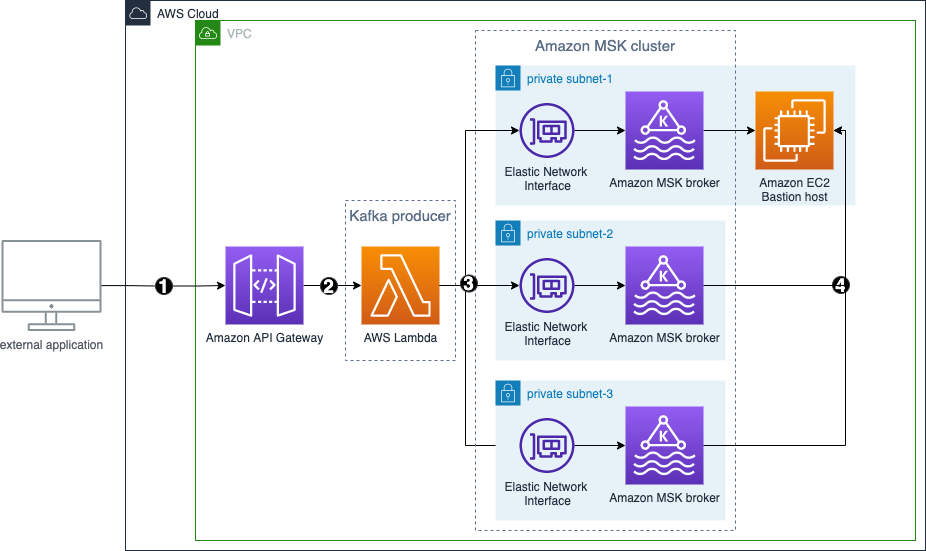
The data flow starts with an Amazon Elastic Compute Cloud (Amazon EC2) client instance that writes records to an MSK topic. As data arrives, an instance of the MongoDB Connector for Apache Kafka writes the data to a collection in the MongoDB Atlas Serverless cluster. For secure connectivity between the two platforms, an AWS PrivateLink connection is created between the MongoDB Atlas cluster and the VPC containing the MSK instance.

This post walks you through the following steps:

  1. Create the serverless MSK cluster.
  2. Create the MongoDB Atlas Serverless cluster.
  3. Configure the MSK plugin.
  4. Create the EC2 client.
  5. Configure an MSK topic.
  6. Configure the MongoDB Connector for Apache Kafka as a sink.

Configure the serverless MSK cluster

To create a serverless MSK cluster, complete the following steps:

  1. On the Amazon MSK console, choose Clusters in the navigation pane.
  2. Choose Create cluster.
  3. For Creation method, select Custom create.
  4. For Cluster name, enter MongoDBMSKCluster.
  5. For Cluster type¸ select Serverless.
  6. Choose Next.Serverless MSK Cluster creation UI
  7. On the Networking page, specify your VPC, Availability Zones, and corresponding subnets.
  8. Note the Availability Zones and subnets to use later.Cluster settings showing VPC and Subnets
  9. Choose Next.
  10. Choose Create cluster.

When the cluster is available, its status becomes Active.

Cluster Available for Use

Create the MongoDB Atlas Serverless cluster

To create a MongoDB Atlas cluster, follow the Getting Started with Atlas tutorial. Note that for the purposes of this post, you need to create a serverless instance.

Create new cluster dialog

After the cluster is created, configure an AWS private endpoint with the following steps:

  1. On the Security menu, choose Network Access.Network Access location in the Security menu
  2. On the Private Endpoint tab, choose Serverless Instance.
    Serverless Instance network access
  3. Choose Create new endpoint.
  4. For Serverless Instance, choose the instance you just created.
  5. Choose Confirm.Create Private Endpoint UI
  6. Provide your VPC endpoint configuration and choose Next.VPC Endpoint Configuration UI
  7. When creating the AWS PrivateLink resource, make sure you specify the exact same VPC and subnets that you used earlier when creating the networking configuration for the serverless MSK instance.
  8. Choose Next.VPC Endpoint Subnet Configuration UI
  9. Follow the instructions on the Finalize page, then choose Confirm after your VPC endpoint is created.

Upon success, the new private endpoint will show up in the list, as shown in the following screenshot.

Network Access Confirmation Page

Configure the MSK Plugin

Next, we create a custom plugin in Amazon MSK using the MongoDB Connector for Apache Kafka. The connector needs to be uploaded to an Amazon Simple Storage Service (Amazon S3) bucket before you can create the plugin. To download the MongoDB Connector for Apache Kafka, refer to Download a Connector JAR File.

  1. On the Amazon MSK console, choose Customized plugins in the navigation pane.
  2. Choose Create custom plugin.
  3. For S3 URI, enter the S3 location of the downloaded connector.
  4. Choose Create custom plugin.

MSK plugin details

Configure an EC2 client

Next, let’s configure an EC2 instance. We use this instance to create the topic and insert data into the topic. For instructions, refer to the section Configure an EC2 client in the post Integrating MongoDB with Amazon Managed Streaming for Apache Kafka (MSK).

Create a topic on the MSK cluster

To create a Kafka topic, we need to install the Kafka CLI first.

  1. On the client EC2 instance, first install Java:

sudo yum install java-1.8.0

  1. Next, run the following command to download Apache Kafka:

wget https://archive.apache.org/dist/kafka/2.6.2/kafka_2.12-2.6.2.tgz

  1. Unpack the tar file using the following command:

tar -xzf kafka_2.12-2.6.2.tgz

The distribution of Kafka includes a bin folder with tools that can be used to manage topics.

  1. Go to the kafka_2.12-2.6.2 directory and issue the following command to create a Kafka topic on the serverless MSK cluster:

bin/kafka-topics.sh --create --topic sandbox_sync2 --bootstrap-server <BOOTSTRAP SERVER> --command-config=bin/client.properties --partitions 2

You can copy the bootstrap server endpoint on the View Client Information page for your serverless MSK cluster.

Bootstrap Server Connection Page

You can configure IAM authentication by following these instructions.

Configure the sink connector

Now, let’s configure a sink connector to send the data to the MongoDB Atlas Serverless instance.

  1. On the Amazon MSK console, choose Connectors in the navigation pane.
  2. Choose Create connector.
  3. Select the plugin you created earlier.
  4. Choose Next.Sink Connector UI
  5. Select the serverless MSK instance that you created earlier.
  6. Enter your connection configuration as the following code:
connector.class=com.mongodb.kafka.connect.MongoSinkConnector
key.converter.schema.enable=false
value.converter.schema.enable=false
database=MongoDBMSKDemo
collection=Sink
tasks.max=1
topics=MongoDBMSKDemo.Source
connection.uri=(MongoDB Atlas Connection String Gos Here) 
value.converter=org.apache.kafka.connect.storage.StringConverter 
key.converter=org.apache.kafka.connect.storage.StringConverter

Make sure that the connection to the MongoDB Atlas Serverless instance is through AWS PrivateLink. For more information, refer to Connecting Applications Securely to a MongoDB Atlas Data Plane with AWS PrivateLink.

  1. In the Access Permissions section, create an AWS Identity and Access Management (IAM) role with the required trust policy.
  2. Choose Next.IAM Role configuration
  3. Specify Amazon CloudWatch Logs as your log delivery option.
  4. Complete your connector.

When the connector status changes to Active, the pipeline is ready.

Connector Confirmation Page

Insert data into the MSK topic

On your EC2 client, insert data into the MSK topic using the kafka-console-producer as follows:

bin/kafka-console-producer.sh --topic sandbox_sync2 --bootstrap-server <BOOTSTRAP SERVER> --producer.config=bin/client.properties

To verify that data successfully flows from the Kafka topic to the serverless MongoDB cluster, we use the MongoDB Atlas UI.

MongoDB Atlas Browse Collections UI

If you run into any issues, be sure to check the log files. In this example, we used CloudWatch to read the events that were generated from Amazon MSK and the MongoDB Connector for Apache Kafka.

CloudWatch Logs UI

Clean up

To avoid incurring future charges, clean up the resources you created. First, delete the MSK cluster, connector, and EC2 instance:

  1. On the Amazon MSK console, choose Clusters in the navigation pane.
  2. Select your cluster and on the Actions menu, choose Delete.
  3. Choose Connectors in the navigation pane.
  4. Select your connector and choose Delete.
  5. Choose Customized plugins in the navigation pane.
  6. Select your plugin and choose Delete.
  7. On the Amazon EC2 console, choose Instances in the navigation pane.
  8. Choose the instance you created.
  9. Choose Instance state, then choose Terminate instance.
  10. On the Amazon VPC console, choose Endpoints in the navigation pane.
  11. Select the endpoint you created and on the Actions menu, choose Delete VPC endpoints.

Now you can delete the Atlas cluster and AWS PrivateLink:

  1. Log in to the Atlas cluster console.
  2. Navigate to the serverless cluster to be deleted.
  3. On the options drop-down menu, choose Terminate.
  4. Navigate to the Network Access section.
  5. Choose the private endpoint.
  6. Select the serverless instance.
  7. On the options drop-down menu, choose Terminate.Endpoint Termination UI

Summary

In this post, we showed you how to build a serverless streaming ingestion pipeline using MSK Serverless and MongoDB Atlas Serverless. With MSK Serverless, you can automatically provision and manage required resources on an as-needed basis. We used a MongoDB connector deployed on MSK Connect to seamlessly integrate the two services, and used an EC2 client to send sample data to the MSK topic. MSK Connect now supports Private DNS hostnames, enabling you to use private domain names between the services. In this post, the connector used the default DNS servers of the VPC to resolve the Availability Zone-specific private DNS name. This AWS PrivateLink configuration allowed secure and private connectivity between the MSK Serverless instance and the MongoDB Atlas Serverless instance.

To continue your learning, check out the following resources:


About the Authors

Igor Alekseev is a Senior Partner Solution Architect at AWS in Data and Analytics domain. In his role Igor is working with strategic partners helping them build complex, AWS-optimized architectures. Prior joining AWS, as a Data/Solution Architect he implemented many projects in Big Data domain, including several data lakes in Hadoop ecosystem. As a Data Engineer he was involved in applying AI/ML to fraud detection and office automation.

Kiran Matty is a Principal Product Manager with Amazon Web Services (AWS) and works with the Amazon Managed Streaming for Apache Kafka (Amazon MSK) team based out of Palo Alto, California. He is passionate about building performant streaming and analytical services that help enterprises realize their critical use cases.

 Babu Srinivasan is a Senior Partner Solutions Architect at MongoDB. In his current role, he is working with AWS to build the technical integrations and reference architectures for the AWS and MongoDB solutions. He has more than two decades of experience in Database and Cloud technologies . He is passionate about providing technical solutions to customers working with multiple Global System Integrators(GSIs) across multiple geographies.

Robert Walters is currently a Senior Product Manager at MongoDB. Previous to MongoDB, Rob spent 17 years at Microsoft working in various roles, including program management on the SQL Server team, consulting, and technical pre-sales. Rob has co-authored three patents for technologies used within SQL Server and was the lead author of several technical books on SQL Server. Rob is currently an active blogger on MongoDB Blogs.

Near-real-time fraud detection using Amazon Redshift Streaming Ingestion with Amazon Kinesis Data Streams and Amazon Redshift ML

Post Syndicated from Praveen Kadipikonda original https://aws.amazon.com/blogs/big-data/near-real-time-fraud-detection-using-amazon-redshift-streaming-ingestion-with-amazon-kinesis-data-streams-and-amazon-redshift-ml/

The importance of data warehouses and analytics performed on data warehouse platforms has been increasing steadily over the years, with many businesses coming to rely on these systems as mission-critical for both short-term operational decision-making and long-term strategic planning. Traditionally, data warehouses are refreshed in batch cycles, for example, monthly, weekly, or daily, so that businesses can derive various insights from them.

Many organizations are realizing that near-real-time data ingestion along with advanced analytics opens up new opportunities. For example, a financial institute can predict if a credit card transaction is fraudulent by running an anomaly detection program in near-real-time mode rather than in batch mode.

In this post, we show how Amazon Redshift can deliver streaming ingestion and machine learning (ML) predictions all in one platform.

Amazon Redshift is a fast, scalable, secure, and fully managed cloud data warehouse that makes it simple and cost-effective to analyze all your data using standard SQL.

Amazon Redshift ML makes it easy for data analysts and database developers to create, train, and apply ML models using familiar SQL commands in Amazon Redshift data warehouses.

We’re excited to launch Amazon Redshift Streaming Ingestion for Amazon Kinesis Data Streams and Amazon Managed Streaming for Apache Kafka (Amazon MSK), which enables you to ingest data directly from a Kinesis data stream or Kafka topic without having to stage the data in Amazon Simple Storage Service (Amazon S3). Amazon Redshift streaming ingestion allows you to achieve low latency in the order of seconds while ingesting hundreds of megabytes of data into your data warehouse.

This post demonstrates how Amazon Redshift, the cloud data warehouse allows you to build near-real-time ML predictions by using Amazon Redshift streaming ingestion and Redshift ML features with familiar SQL language.

Solution overview

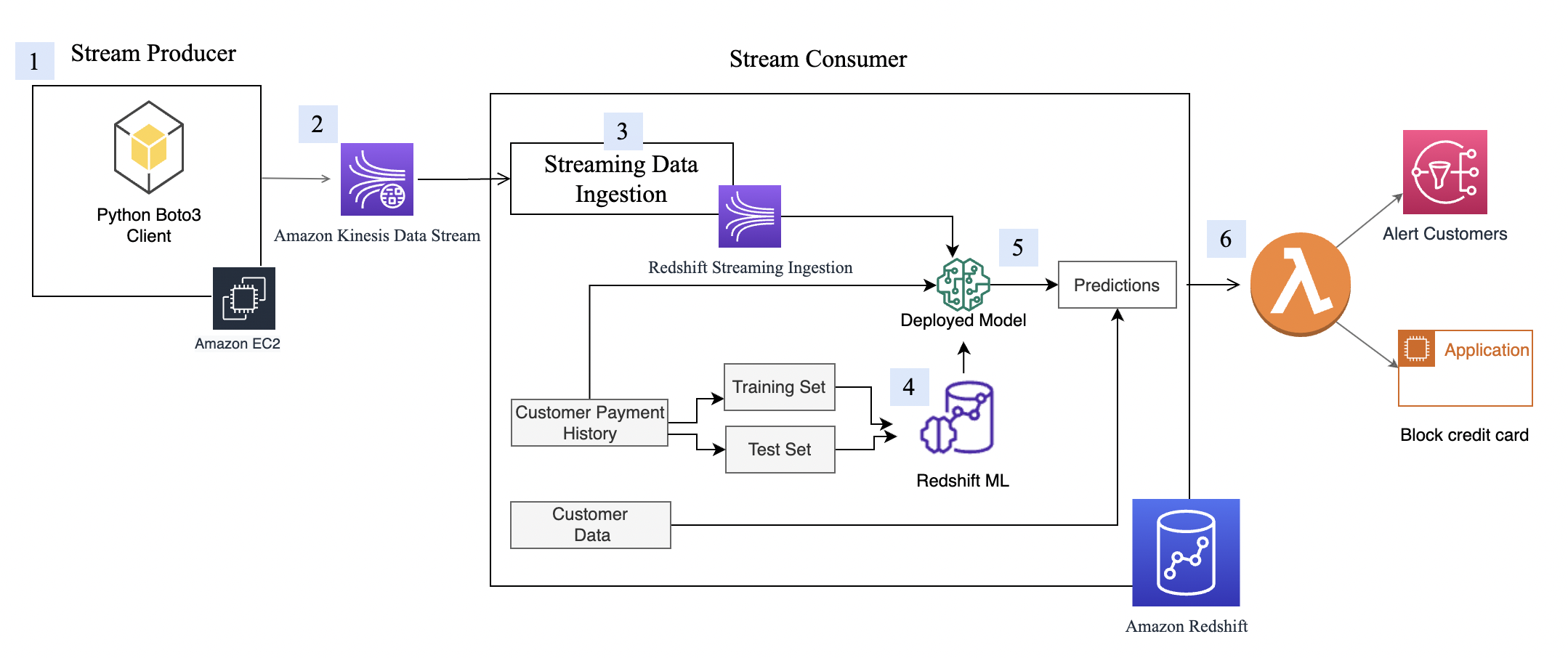
By following the steps outlined in this post, you’ll be able to set up a producer streamer application on an Amazon Elastic Compute Cloud (Amazon EC2) instance that simulates credit card transactions and pushes data to Kinesis Data Streams in real time. You set up an Amazon Redshift Streaming Ingestion materialized view on Amazon Redshift, where streaming data is received. You train and build a Redshift ML model to generate real-time inferences against the streaming data.

The following diagram illustrates the architecture and process flow.

The step-by-step process is as follows:

  1. The EC2 instance simulates a credit card transaction application, which inserts credit card transactions into the Kinesis data stream.
  2. The data stream stores the incoming credit card transaction data.
  3. An Amazon Redshift Streaming Ingestion materialized view is created on top of the data stream, which automatically ingests streaming data into Amazon Redshift.
  4. You build, train, and deploy an ML model using Redshift ML. The Redshift ML model is trained using historical transactional data.
  5. You transform the streaming data and generate ML predictions.
  6. You can alert customers or update the application to mitigate risk.

This walkthrough uses credit card transaction streaming data. The credit card transaction data is fictitious and is based on a simulator. The customer dataset is also fictitious and is generated with some random data functions.

Prerequisites

  1. Create an Amazon Redshift cluster.
  2. Configure the cluster to use Redshift ML.
  3. Create an AWS Identity and Access Management (IAM) user.
  4. Update the IAM role attached to the Redshift cluster to include permissions to access the Kinesis data stream. For more information about the required policy, refer to Getting started with streaming ingestion.
  5. Create an m5.4xlarge EC2 instance. We tested Producer application with m5.4xlarge instance but you are free to use other instance type. When creating the instance, use the amzn2-ami-kernel-5.10-hvm-2.0.20220426.0-x86_64-gp2 AMI.
  6. To make sure that Python3 is installed in the EC2 instance, run the following command to verity your Python version (note that the data extraction script only works on Python 3):
python3 --version
  1. Install the following dependent packages to run the simulator program:
sudo yum install python3-pip
pip3 install numpy
pip3 install pandas
pip3 install matplotlib
pip3 install seaborn
pip3 install boto3
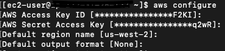
  1. Configure Amazon EC2 using the variables like AWS credentials generated for IAM user created in step 3 above. The following screenshot shows an example using aws configure.

Set up Kinesis Data Streams

Amazon Kinesis Data Streams is a massively scalable and durable real-time data streaming service. It can continuously capture gigabytes of data per second from hundreds of thousands of sources, such as website clickstreams, database event streams, financial transactions, social media feeds, IT logs, and location-tracking events. The data collected is available in milliseconds to enable real-time analytics use cases such as real-time dashboards, real-time anomaly detection, dynamic pricing, and more. We use Kinesis Data Streams because it’s a serverless solution that can scale based on usage.

Create a Kinesis data stream

First, you need to create a Kinesis data stream to receive the streaming data:

  1. On the Amazon Kinesis console, choose Data streams in the navigation pane.
  2. Choose Create data stream.
  3. For Data stream name, enter cust-payment-txn-stream.
  4. For Capacity mode, select On-demand.
  5. For the rest of the options, choose the default options and follow through the prompts to complete the setup.
  6. Capture the ARN for the created data stream to use in the next section when defining your IAM policy.

Streaming ARN Highlight

Set up permissions

For a streaming application to write to Kinesis Data Streams, the application needs to have access to Kinesis. You can use the following policy statement to grant the simulator process that you set up in next section access to the data stream. Use the ARN of the data stream that you saved in the previous step.

{
"Version": "2012-10-17",
"Statement": [
{
"Sid": "Stmt123",
"Effect": "Allow",
"Action": [
"kinesis:DescribeStream",
"kinesis:PutRecord",
"kinesis:PutRecords",
"kinesis:GetShardIterator",
"kinesis:GetRecords",
"kinesis:ListShards",
"kinesis:DescribeStreamSummary"
],
"Resource": [
"arn:aws:kinesis:us-west-2:xxxxxxxxxxxx:stream/cust-payment-txn-stream"
]
}
]
}

Configure the stream producer

Before we can consume streaming data in Amazon Redshift, we need a streaming data source that writes data to the Kinesis data stream. This post uses a custom-built data generator and the AWS SDK for Python (Boto3) to publish the data to the data stream. For setup instructions, refer to Producer Simulator. This simulator process publishes streaming data to the data stream created in the previous step (cust-payment-txn-stream).

Configure the stream consumer

This section talks about configuring the stream consumer (the Amazon Redshift streaming ingestion view).

Amazon Redshift Streaming Ingestion provides low-latency, high-speed ingestion of streaming data from Kinesis Data Streams into an Amazon Redshift materialized view. You can configure your Amazon Redshift cluster to enable streaming ingestion and create a materialized view with auto refresh, using SQL statements, as described in Creating materialized views in Amazon Redshift. The automatic materialized view refresh process will ingest streaming data at hundreds of megabytes of data per second from Kinesis Data Streams into Amazon Redshift. This results in fast access to external data that is quickly refreshed.

After creating the materialized view, you can access your data from the data stream using SQL and simplify your data pipelines by creating materialized views directly on top of the stream.

Complete the following steps to configure an Amazon Redshift streaming materialized view:

  1. On the IAM console, choose policies in the navigation pane.
  2. Choose Create policy.
  3. Create a new IAM policy called KinesisStreamPolicy.  For the streaming policy definition, see Getting started with streaming ingestion.
  4. In the navigation pane, choose Roles.
  5. Choose Create role.
  6. Select AWS service and choose Redshift and Redshift customizable.
  7. Create a new role called redshift-streaming-role and attach the policy KinesisStreamPolicy.
  8. Create an external schema to map to Kinesis Data Streams :
CREATE EXTERNAL SCHEMA custpaytxn
FROM KINESIS IAM_ROLE 'arn:aws:iam::386xxxxxxxxx:role/redshift-streaming-role';

Now you can create a materialized view to consume the stream data. You can use the SUPER data type to store the payload as is, in JSON format, or use Amazon Redshift JSON functions to parse the JSON data into individual columns. For this post, we use the second method because the schema is well defined.

  1. Create the streaming ingestion materialized view cust_payment_tx_stream. By specifying AUTO REFRESH YES in the following code, you can enable automatic refresh of the streaming ingestion view, which saves time by avoiding building data pipelines:
CREATE MATERIALIZED VIEW cust_payment_tx_stream
AUTO REFRESH YES
AS
SELECT approximate_arrival_timestamp ,
partition_key,
shard_id,
sequence_number,
json_extract_path_text(from_varbyte(kinesis_data, 'utf-8'),'TRANSACTION_ID')::bigint as TRANSACTION_ID,
json_extract_path_text(from_varbyte(kinesis_data, 'utf-8'),'TX_DATETIME')::character(50) as TX_DATETIME,
json_extract_path_text(from_varbyte(kinesis_data, 'utf-8'),'CUSTOMER_ID')::int as CUSTOMER_ID,
json_extract_path_text(from_varbyte(kinesis_data, 'utf-8'),'TERMINAL_ID')::int as TERMINAL_ID,
json_extract_path_text(from_varbyte(kinesis_data, 'utf-8'),'TX_AMOUNT')::decimal(18,2) as TX_AMOUNT,
json_extract_path_text(from_varbyte(kinesis_data, 'utf-8'),'TX_TIME_SECONDS')::int as TX_TIME_SECONDS,
json_extract_path_text(from_varbyte(kinesis_data, 'utf-8'),'TX_TIME_DAYS')::int as TX_TIME_DAYS
FROM custpaytxn."cust-payment-txn-stream"
Where is_utf8(kinesis_data) AND can_json_parse(kinesis_data);

Note that json_extract_path_text has a length limitation of 64 KB. Also from_varbye filters records larger than 65KB.

  1. Refresh the data.

The Amazon Redshift streaming materialized view is auto refreshed by Amazon Redshift for you. This way, you don’t need worry about data staleness. With materialized view auto refresh, data is automatically loaded into Amazon Redshift as it becomes available in the stream. If you choose to manually perform this operation, use the following command:

REFRESH MATERIALIZED VIEW cust_payment_tx_stream ;
  1. Now let’s query the streaming materialized view to see sample data:
Select * from cust_payment_tx_stream limit 10;

  1. Let’s check how many records are in the streaming view now:
Select count(*) as stream_rec_count from cust_payment_tx_stream;

Now you have finished setting up the Amazon Redshift streaming ingestion view, which is continuously updated with incoming credit card transaction data. In my setup, I see that around 67,000 records have been pulled into the streaming view at the time when I ran my select count query. This number could be different for you.

Redshift ML

With Redshift ML, you can bring a pre-trained ML model or build one natively. For more information, refer to Using machine learning in Amazon Redshift.

In this post, we train and build an ML model using a historical dataset. The data contains a tx_fraud field that flags a historical transaction as fraudulent or not. We build a supervised ML model using Redshift Auto ML, which learns from this dataset and predicts incoming transactions when those are run through the prediction functions.

In the following sections, we show how to set up the historical dataset and customer data.

Load the historical dataset

The historical table has more fields than what the streaming data source has. These fields contain the customer’s most recent spend and terminal risk score, like number of fraudulent transactions computed by transforming streaming data. There are also categorical variables like weekend transactions or nighttime transactions.

To load the historical data, run the commands using the Amazon Redshift query editor.

Create the transaction history table with the following code. The DDL can also be found on GitHub.

CREATE TABLE cust_payment_tx_history
(
TRANSACTION_ID integer,
TX_DATETIME timestamp,
CUSTOMER_ID integer,
TERMINAL_ID integer,
TX_AMOUNT decimal(9,2),
TX_TIME_SECONDS integer,
TX_TIME_DAYS integer,
TX_FRAUD integer,
TX_FRAUD_SCENARIO integer,
TX_DURING_WEEKEND integer,
TX_DURING_NIGHT integer,
CUSTOMER_ID_NB_TX_1DAY_WINDOW decimal(9,2),
CUSTOMER_ID_AVG_AMOUNT_1DAY_WINDOW decimal(9,2),
CUSTOMER_ID_NB_TX_7DAY_WINDOW decimal(9,2),
CUSTOMER_ID_AVG_AMOUNT_7DAY_WINDOW decimal(9,2),
CUSTOMER_ID_NB_TX_30DAY_WINDOW decimal(9,2),
CUSTOMER_ID_AVG_AMOUNT_30DAY_WINDOW decimal(9,2),
TERMINAL_ID_NB_TX_1DAY_WINDOW decimal(9,2),
TERMINAL_ID_RISK_1DAY_WINDOW decimal(9,2),
TERMINAL_ID_NB_TX_7DAY_WINDOW decimal(9,2),
TERMINAL_ID_RISK_7DAY_WINDOW decimal(9,2),
TERMINAL_ID_NB_TX_30DAY_WINDOW decimal(9,2),
TERMINAL_ID_RISK_30DAY_WINDOW decimal(9,2)
);
Copy cust_payment_tx_history
FROM 's3://redshift-demos/redshiftml-reinvent/2022/ant312/credit-card-transactions/credit_card_transactions_transformed_balanced.csv'
iam_role default
ignoreheader 1
csv ;

Let’s check how many transactions are loaded:

select count(1) from cust_payment_tx_history;

Check the monthly fraud and non-fraud transactions trend:

SELECT to_char(tx_datetime, 'YYYYMM') as YearMonth,
sum(case when tx_fraud=1 then 1 else 0 end) as fraud_tx,
sum(case when tx_fraud=0 then 1 else 0 end) as non_fraud_tx,
count(*) as total_tx
FROM cust_payment_tx_history
GROUP BY YearMonth;

Create and load customer data

Now we create the customer table and load data, which contains the email and phone number of the customer. The following code creates the table, loads the data, and samples the table. The table DDL is available on GitHub.

CREATE TABLE public."customer_info"(customer_id bigint NOT NULL encode az64,
job_title character varying(500) encode lzo,
email_address character varying(100) encode lzo,
full_name character varying(200) encode lzo,
phone_number character varying(20) encode lzo,
city varchar(50),
state varchar(50)
);
COPY customer_info
FROM 's3://redshift-demos/redshiftml-reinvent/2022/ant312/customer-data/Customer_Data.csv'
IGNOREHEADER 1
IAM_ROLE default CSV;
Select count(1) from customer_info;

Our test data has about 5,000 customers. The following screenshot shows sample customer data.

Build an ML model

Our historical card transaction table has 6 months of data, which we now use to train and test the ML model.

The model takes the following fields as input:

TX_DURING_WEEKEND ,
TX_AMOUNT,
TX_DURING_NIGHT ,
CUSTOMER_ID_NB_TX_1DAY_WINDOW ,
CUSTOMER_ID_AVG_AMOUNT_1DAY_WINDOW ,
CUSTOMER_ID_NB_TX_7DAY_WINDOW ,
CUSTOMER_ID_AVG_AMOUNT_7DAY_WINDOW ,
CUSTOMER_ID_NB_TX_30DAY_WINDOW ,
CUSTOMER_ID_AVG_AMOUNT_30DAY_WINDOW ,
TERMINAL_ID_NB_TX_1DAY_WINDOW ,
TERMINAL_ID_RISK_1DAY_WINDOW ,
TERMINAL_ID_NB_TX_7DAY_WINDOW ,
TERMINAL_ID_RISK_7DAY_WINDOW ,
TERMINAL_ID_NB_TX_30DAY_WINDOW ,
TERMINAL_ID_RISK_30DAY_WINDOW

We get tx_fraud as output.

We split this data into training and test datasets. Transactions from 2022-04-01 to 2022-07-31 are for the training set. Transactions from 2022-08-01 to 2022-09-30 are used for the test set.

Let’s create the ML model using the familiar SQL CREATE MODEL statement. We use a basic form of the Redshift ML command. The following method uses Amazon SageMaker Autopilot, which performs data preparation, feature engineering, model selection, and training automatically for you. Provide the name of your S3 bucket containing the code.

CREATE MODEL cust_cc_txn_fd
FROM (
SELECT TX_AMOUNT ,
TX_FRAUD ,
TX_DURING_WEEKEND ,
TX_DURING_NIGHT ,
CUSTOMER_ID_NB_TX_1DAY_WINDOW ,
CUSTOMER_ID_AVG_AMOUNT_1DAY_WINDOW ,
CUSTOMER_ID_NB_TX_7DAY_WINDOW ,
CUSTOMER_ID_AVG_AMOUNT_7DAY_WINDOW ,
CUSTOMER_ID_NB_TX_30DAY_WINDOW ,
CUSTOMER_ID_AVG_AMOUNT_30DAY_WINDOW ,
TERMINAL_ID_NB_TX_1DAY_WINDOW ,
TERMINAL_ID_RISK_1DAY_WINDOW ,
TERMINAL_ID_NB_TX_7DAY_WINDOW ,
TERMINAL_ID_RISK_7DAY_WINDOW ,
TERMINAL_ID_NB_TX_30DAY_WINDOW ,
TERMINAL_ID_RISK_30DAY_WINDOW
FROM cust_payment_tx_history
WHERE cast(tx_datetime as date) between '2022-06-01' and '2022-09-30'
) TARGET tx_fraud
FUNCTION fn_customer_cc_fd
IAM_ROLE default
SETTINGS (
S3_BUCKET '<replace this with your s3 bucket name>',
s3_garbage_collect off,
max_runtime 3600
);

I call the ML model as Cust_cc_txn_fd, and the prediction function as fn_customer_cc_fd. The FROM clause shows the input columns from the historical table public.cust_payment_tx_history. The target parameter is set to tx_fraud, which is the target variable that we’re trying to predict. IAM_Role is set to default because the cluster is configured with this role; if not, you have to provide your Amazon Redshift cluster IAM role ARN. I set the max_runtime to 3,600 seconds, which is the time we give to SageMaker to complete the process. Redshift ML deploys the best model that is identified in this time frame.

Depending on the complexity of the model and the amount of data, it can take some time for the model to be available. If you find your model selection is not completing, increase the value for max_runtime. You can set a max value of 9999.

The CREATE MODEL command is run asynchronously, which means it runs in the background. You can use the SHOW MODEL command to see the status of the model. When the status shows as Ready, it means the model is trained and deployed.

show model cust_cc_txn_fd;

The following screenshots show our output.

From the output, I see that the model has been correctly recognized as BinaryClassification, and F1 has been selected as the objective. The F1 score is a metric that considers both precision and recall. It returns a value between 1 (perfect precision and recall) and 0 (lowest possible score). In my case, it’s 0.91. The higher the value, the better the model performance.

Let’s test this model with the test dataset. Run the following command, which retrieves sample predictions:

SELECT
tx_fraud ,
fn_customer_cc_fd(
TX_AMOUNT ,
TX_DURING_WEEKEND ,
TX_DURING_NIGHT ,
CUSTOMER_ID_NB_TX_1DAY_WINDOW ,
CUSTOMER_ID_AVG_AMOUNT_1DAY_WINDOW ,
CUSTOMER_ID_NB_TX_7DAY_WINDOW ,
CUSTOMER_ID_AVG_AMOUNT_7DAY_WINDOW ,
CUSTOMER_ID_NB_TX_30DAY_WINDOW ,
CUSTOMER_ID_AVG_AMOUNT_30DAY_WINDOW ,
TERMINAL_ID_NB_TX_1DAY_WINDOW ,
TERMINAL_ID_RISK_1DAY_WINDOW ,
TERMINAL_ID_NB_TX_7DAY_WINDOW ,
TERMINAL_ID_RISK_7DAY_WINDOW ,
TERMINAL_ID_NB_TX_30DAY_WINDOW ,
TERMINAL_ID_RISK_30DAY_WINDOW )
FROM cust_payment_tx_history
WHERE cast(tx_datetime as date) >= '2022-10-01'
limit 10 ;

We see that some values are matching and some are not. Let’s compare predictions to the ground truth:

SELECT
tx_fraud ,
fn_customer_cc_fd(
TX_AMOUNT ,
TX_DURING_WEEKEND ,
TX_DURING_NIGHT ,
CUSTOMER_ID_NB_TX_1DAY_WINDOW ,
CUSTOMER_ID_AVG_AMOUNT_1DAY_WINDOW ,
CUSTOMER_ID_NB_TX_7DAY_WINDOW ,
CUSTOMER_ID_AVG_AMOUNT_7DAY_WINDOW ,
CUSTOMER_ID_NB_TX_30DAY_WINDOW ,
CUSTOMER_ID_AVG_AMOUNT_30DAY_WINDOW ,
TERMINAL_ID_NB_TX_1DAY_WINDOW ,
TERMINAL_ID_RISK_1DAY_WINDOW ,
TERMINAL_ID_NB_TX_7DAY_WINDOW ,
TERMINAL_ID_RISK_7DAY_WINDOW ,
TERMINAL_ID_NB_TX_30DAY_WINDOW ,
TERMINAL_ID_RISK_30DAY_WINDOW
) as prediction, count(*) as values
FROM public.cust_payment_tx_history
WHERE cast(tx_datetime as date) >= '2022-08-01'
Group by 1,2 ;

We validated that the model is working and the F1 score is good. Let’s move on to generating predictions on streaming data.

Predict fraudulent transactions

Because the Redshift ML model is ready to use, we can use it to run the predictions against streaming data ingestion. The historical dataset has more fields than what we have in the streaming data source, but they’re just recency and frequency metrics around the customer and terminal risk for a fraudulent transaction.

We can apply the transformations on top of the streaming data very easily by embedding the SQL inside the views. Create the first view, which aggregates streaming data at the customer level. Then create the second view, which aggregates streaming data at terminal level, and the third view, which combines incoming transactional data with customer and terminal aggregated data and calls the prediction function all in one place. The code for the third view is as follows:

CREATE VIEW public.cust_payment_tx_fraud_predictions
as
select a.approximate_arrival_timestamp,
d.full_name , d.email_address, d.phone_number,
a.TRANSACTION_ID, a.TX_DATETIME, a.CUSTOMER_ID, a.TERMINAL_ID,
a.TX_AMOUNT ,
a.TX_TIME_SECONDS ,
a.TX_TIME_DAYS ,
public.fn_customer_cc_fd(a.TX_AMOUNT ,
a.TX_DURING_WEEKEND,
a.TX_DURING_NIGHT,
c.CUSTOMER_ID_NB_TX_1DAY_WINDOW ,
c.CUSTOMER_ID_AVG_AMOUNT_1DAY_WINDOW ,
c.CUSTOMER_ID_NB_TX_7DAY_WINDOW ,
c.CUSTOMER_ID_AVG_AMOUNT_7DAY_WINDOW ,
c.CUSTOMER_ID_NB_TX_30DAY_WINDOW ,
c.CUSTOMER_ID_AVG_AMOUNT_30DAY_WINDOW ,
t.TERMINAL_ID_NB_TX_1DAY_WINDOW ,
t.TERMINAL_ID_RISK_1DAY_WINDOW ,
t.TERMINAL_ID_NB_TX_7DAY_WINDOW ,
t.TERMINAL_ID_RISK_7DAY_WINDOW ,
t.TERMINAL_ID_NB_TX_30DAY_WINDOW ,
t.TERMINAL_ID_RISK_30DAY_WINDOW ) Fraud_prediction
From
(select
Approximate_arrival_timestamp,
TRANSACTION_ID, TX_DATETIME, CUSTOMER_ID, TERMINAL_ID,
TX_AMOUNT ,
TX_TIME_SECONDS ,
TX_TIME_DAYS ,
case when extract(dow from cast(TX_DATETIME as timestamp)) in (1,7) then 1 else 0 end as TX_DURING_WEEKEND,
case when extract(hour from cast(TX_DATETIME as timestamp)) between 00 and 06 then 1 else 0 end as TX_DURING_NIGHT
FROM cust_payment_tx_stream) a
join terminal_transformations t
on a.terminal_id = t.terminal_id
join customer_transformations c
on a.customer_id = c.customer_id
join customer_info d
on a.customer_id = d.customer_id
;

Run a SELECT statement on the view:

select * from
cust_payment_tx_fraud_predictions
where Fraud_prediction = 1;

As you run the SELECT statement repeatedly, the latest credit card transactions go through transformations and ML predictions in near-real time.

This demonstrates the power of Amazon Redshift—with easy-to-use SQL commands, you can transform streaming data by applying complex window functions and apply an ML model to predict fraudulent transactions all in one step, without building complex data pipelines or building and managing additional infrastructure.

Expand the solution

Because the data streams in and ML predictions are made in near-real time, you can build business processes for alerting your customer using Amazon Simple Notification Service (Amazon SNS), or you can lock the customer’s credit card account in an operational system.

This post doesn’t go into the details of these operations, but if you’re interested in learning more about building event-driven solutions using Amazon Redshift, refer to the following GitHub repository.

Clean up

To avoid incurring future charges, delete the resources that were created as part of this post.

Conclusion

In this post, we demonstrated how to set up a Kinesis data stream, configure a producer and publish data to streams, and then create an Amazon Redshift Streaming Ingestion view and query the data in Amazon Redshift. After the data was in the Amazon Redshift cluster, we demonstrated how to train an ML model and build a prediction function and apply it against the streaming data to generate predictions near-real time.

If you have any feedback or questions, please leave them in the comments.


About the Authors

Bhanu Pittampally is an Analytics Specialist Solutions Architect based out of Dallas. He specializes in building analytic solutions. His background is in data warehouses—architecture, development, and administration. He has been in the data and analytics field for over 15 years.

Praveen Kadipikonda is a Senior Analytics Specialist Solutions Architect at AWS based out of Dallas. He helps customers build efficient, performant, and scalable analytic solutions. He has worked with building databases and data warehouse solutions for over 15 years.

Ritesh Kumar Sinha is an Analytics Specialist Solutions Architect based out of San Francisco. He has helped customers build scalable data warehousing and big data solutions for over 16 years. He loves to design and build efficient end-to-end solutions on AWS. In his spare time, he loves reading, walking, and doing yoga.

Analyze real-time streaming data in Amazon MSK with Amazon Athena

Post Syndicated from Scott Rigney original https://aws.amazon.com/blogs/big-data/analyze-real-time-streaming-data-in-amazon-msk-with-amazon-athena/

Recent advances in ease of use and scalability have made streaming data easier to generate and use for real-time decision-making. Coupled with market forces that have forced businesses to react more quickly to industry changes, more and more organizations today are turning to streaming data to fuel innovation and agility.

Amazon Managed Streaming for Apache Kafka (MSK) is a fully managed service that makes it easy to build and run applications that use Apache Kafka, an open-source distributed event streaming platform designed for high-performance data pipelines, streaming analytics, data integration, and mission-critical applications. With Amazon MSK, you can capture real-time data from a wide range of sources such as database change events or web application user clickstreams. Since Kafka is highly optimized for writing and reading fresh data, it’s a great fit for operational reporting. However, gaining insight from this data often requires a specialized stream processing layer to write streaming records to a storage medium like Amazon S3, where it can be accessed by analysts, data scientists, and data engineers for historical analysis and visualization using tools like Amazon QuickSight.

When you want to analyze data where it lives and without developing separate pipelines and jobs, a popular choice is Amazon Athena. With Athena, you can use your existing SQL knowledge to extract insights from a wide range of data sources without learning a new language, developing scripts to extract (and duplicate) data, or managing infrastructure. Athena supports over 25 connectors to popular data sources including Amazon DynamoDB and Amazon Redshift which give data analysts, data engineers, and data scientists the flexibility to run SQL queries on data stored in databases running on-premises or in the cloud alongside data stored in Amazon S3. With Athena, there’s no data movement and you pay only for the queries you run.

What’s new

Starting today, you can now use Athena to query streaming data in MSK and self-managed Apache Kafka. This enables you to run analytical queries on real-time data held in Kafka topics and join that data with other Kafka topics as well as other data in your Amazon S3 data lake – all without the need for separate processes to first store the data on Amazon S3.

Solution overview

In this post, we show you how to get started with real-time SQL analytics using Athena and its connector for MSK. The process involves:

  1. Registering the schema of your streaming data with AWS Glue Schema Registry. Schema Registry is a feature of AWS Glue that allows you to validate and reliably evolve streaming data against JSON schemas. It can also serialize data into a compressed format, which helps you save on data transfer and storage costs.
  2. Creating a new instance of the Amazon Athena MSK Connector. Athena connectors are pre-built applications that run as serverless AWS Lambda applications, so there’s no need for standalone data export processes.
  3. Using the Athena console to run interactive SQL queries on your Kafka topics.

Get started with Athena’s connector for Amazon MSK

In this section, we’ll cover the steps necessary to set up your MSK cluster to work with Athena to run SQL queries on your Kafka topics.

Prerequisites

This post assumes you have a serverless or provisioned MSK cluster set up to receive streaming messages from a producing application. For information, see Setting up Amazon MSK and Getting started using Amazon MSK in the Amazon Managed Streaming for Apache Kafka Developer Guide.

You’ll also need to set up a VPC and a security group before you use the Athena connector for MSK. For more information, see Creating a VPC for a data source connector. Note that with MSK Serverless, VPCs and security groups are created automatically, so you can get started quickly.

Define the schema of your Kafka topics with AWS Glue Schema Registry

To run SQL queries on your Kafka topics, you’ll first need to define the schema of your topics as Athena uses this metadata for query planning. AWS Glue makes it easy to do this with its Schema Registry feature for streaming data sources.

Schema Registry allows you to centrally discover, control, and evolve streaming data schemas for use in analytics applications such as Athena. With AWS Glue Schema Registry, you can manage and enforce schemas on your data streaming applications using convenient integrations with Apache Kafka. To learn more, see AWS Glue Schema Registry and Getting started with Schema Registry.

If configured to do so, the producer of data can auto-register its schema and changes to it with AWS Glue. This is especially useful in use cases where the contents of the data is likely to change over time. However, you can also specify the schema manually and will resemble the following JSON structure.

{
  "tableName": "orders",
  "schemaName": "customer_schema",
  "topicName": "orders",
  "message": {
    "dataFormat": "json",
    "fields": [
      {
        "name": "customer_id",
        "mapping": "customer_id",
        "type": "VARCHAR"
      },
      {
        "name": "item_id",
        "mapping": "item_id",
        "type": "INTEGER"
      }
    ]
  }
}

When setting up your Schema Registry, be sure to give it an easy-to-remember name, such as customer_schema, because you’ll reference it within SQL queries as you’ll see later on. For additional information on schema set up, see Schema examples for the AWS Glue Schema Registry.

Configure the Athena connector for MSK

With your schema registered with Glue, the next step is to set up the Athena connector for MSK. We recommend using the Athena console for this step. For more background on the steps involved, see Deploying a connector and connecting to a data source.

In Athena, federated data source connectors are applications that run on AWS Lambda and handle communication between your target data source and Athena. When a query runs on a federated source, Athena calls the Lambda function and tasks it with running the parts of your query that are specific to that source. To learn more about the query execution workflow, see Using Amazon Athena Federated Query in the Amazon Athena User Guide.

Start by accessing the Athena console and selecting Data sources on the left navigation, then choose Create data source:

Next, search for and select Amazon MSK from the available connectors and select Next.

In Data source details, give your connector a name, like msk, that’s easy to remember and reference in your future SQL queries. Under Connection details section, select Create Lambda function. This will bring you to the AWS Lambda console where you’ll provide additional configuration properties.

In the Lambda application configuration screen (not shown), you’ll provide the Application settings for your connector. To do this, you’ll need a few properties from your MSK cluster and schema registered in Glue.

On another browser tab, use the MSK console to navigate to your MSK cluster and then select the Properties tab. Here you’ll see the VPC subnets and security group IDs from your MSK cluster which you’ll provide in the SubnetIds and SecurityGroupIds fields in the Athena connector’s Application settings form. You can find the value for KafkaEndpoint by clicking View client information.

In the AWS Glue console, navigate to your Schema Registry to find the GlueRegistryArn for the schema you wish to use with this connector.

After providing these and the other required values, click Deploy.

Return to the Athena console and enter the name of the Lambda function you just created in the Connection details box, then click Create data source.

Run queries on streaming data using Athena

With your MSK data connector set up, you can now run SQL queries on the data. Let’s explore a few use cases in more detail.

Use case: interactive analysis

If you want to run queries that aggregate, group, or filter your MSK data, you can run interactive queries using Athena. These queries will run against the current state of your Kafka topics at the time the query was submitted.

Before running any queries, it may be helpful to validate the schema and data types available within your Kafka topics. To do this, run the DESCRIBE command on your Kafka topic, which appears in Athena as a table, as shown below. In this query, the orders table corresponds to the topic you specified in the Schema Registry.

DESCRIBE msk.customer_schema.orders

Now that you know the contents of your topic, you can begin to develop analytical queries. A sample query for a hypothetical Kafka topic containing e-commerce order data is shown below:

SELECT customer_id, SUM(order_total)
FROM msk.customer_schema.orders
GROUP BY customer_id

Because the orders table (and underlying Kafka topic) can contain an unbounded stream of data, the query above is likely to return a different value for SUM(order_total) with each execution of the query.

If you have data in one topic that you need to join with another topic, you can do that too:

SELECT t1.order_id, t2.item_id
FROM msk.customer_schema.orders as t1
JOIN msk.customer_schema.items as t2
ON t1.id = t2.id

Use case: ingesting streaming data to a table on Amazon S3

Federated queries run against the underlying data source which ensures interactive queries, like the ones above, are evaluated against the current state of your data. One consideration is that repeatedly running federated queries can put additional load on the underlying source. If you plan to perform multiple queries on the same source data, you can use Athena’s CREATE TABLE AS SELECT, also known as CTAS, to store the results of a SELECT query in a table on Amazon S3. You can then run queries on your newly created table without going back to the underlying source each time.

CREATE TABLE my_kafka_data
WITH (format = 'Parquet', 
      write_compression = 'SNAPPY')
AS
SELECT order_id, item_id, timestamp
FROM msk.customer_schema.orders

If you plan to do additional downstream analysis on this data, for example within dashboards on Amazon QuickSight, you can enhance the solution above by periodically adding new data to your table. To learn more, see Using CTAS and INSERT INTO for ETL and data analysis. Another benefit of this approach is that you can secure these tables with row-, column-, and table-level data governance policies powered by AWS Lake Formation to ensure only authorized users can access your table.

What else can you do?

With Athena, you can use your existing SQL knowledge to run federated queries that generate insights from a wide range of data sources without learning a new language, developing scripts to extract (and duplicate) data, or managing infrastructure. Athena provides additional integrations with other AWS services and popular analytics tools and SQL IDEs that allow you to do much more with your data. For example, you can:

  • Visualize the data in business intelligence applications like Amazon QuickSight
  • Design event-driven data processing workflows with Athena’s integration with AWS Step Functions
  • Unify multiple data sources to produce rich input features for machine learning in Amazon SageMaker

Conclusion

In this post, we learned about the newly released Athena connector for Amazon MSK. With it, you can run interactive queries on data held in Kafka topics running in MSK or self-managed Apache Kafka. This helps you bring real-time insights to dashboards or enable point-in-time analysis of streaming data to answer time-sensitive business questions. We also covered how to periodically ingest new streaming data into Amazon S3 without the need for a separate sink process. This simplifies recurring analysis of your data without incurring round-trip queries to your underlying Kafka clusters and makes it possible to secure the data with access rules powered by Lake Formation.

We encourage you to evaluate Athena and federated queries on your next analytics project. For help getting started, we recommend the following resources:


About the authors

Scott Rigney is a Senior Technical Product Manager with Amazon Web Services (AWS) and works with the Amazon Athena team based out of Arlington, Virginia. He is passionate about building analytics products that enable enterprises to make data-driven decisions.

Kiran Matty is a Principal Product Manager with Amazon Web Services (AWS) and works with the Amazon Managed Streaming for Apache Kafka (Amazon MSK) team based out of Palo Alto, California. He is passionate about building performant streaming and analytical services that help enterprises realize their critical use cases.

Gain visibility into your Amazon MSK cluster by deploying the Conduktor Platform

Post Syndicated from Stéphane Maarek original https://aws.amazon.com/blogs/big-data/gain-visibility-into-your-amazon-msk-cluster-by-deploying-the-conduktor-platform/

This is a guest post by AWS Data Hero and co-founder of Conduktor, Stephane Maarek.

Deploying Apache Kafka on AWS is now easier, thanks to Amazon Managed Streaming for Apache Kafka (Amazon MSK). In a few clicks, it provides you with a production-ready Kafka cluster on which you can run your applications and create data streams.

Apache Kafka is an open-source project, and no official user interfaces are available. The lack of visibility into Apache Kafka is a factor in the slow development of applications.

The recent announcement of the Conduktor Platform makes Amazon MSK operations simple, and you can solve Kafka issues end to end with solutions for testing, monitoring, data quality, governance, and security.

You can use the Conduktor Platform to monitor both types of MSK clusters, provisioned and serverless. In this post, we demonstrate how to use AWS Identity and Access Management (IAM) based security to administer our MSK cluster.

Solution overview

We look at how we can deploy the Conduktor Platform on Amazon MSK in a production-ready deployment so you can try it out today.

The solution is fully serverless and customizable. Everything is deployed using AWS CloudFormation templates.

The source code and CloudFormation templates used in this post are available in the GitHub repo.

To implement this solution, we complete the following high-level steps:

  1. Deploy a CloudFormation template to create our customized Docker image for the Conduktor Platform using AWS CodeBuild.
  2. Optionally, deploy an MSK cluster in provisioned or serverless mode using a CloudFormation template.
  3. Deploy the Conduktor Platform as an AWS Fargate container against our MSK cluster using a CloudFormation template.

Create a customized configuration for the Conduktor Platform

The Conduktor Platform uses a YAML configuration file to define the cluster connection endpoints. Therefore, we must create a customized Docker image of the Conduktor Platform that is able to connect to a cluster on Amazon MSK with a customized YAML file. For this, we use CodeBuild, and we store our configuration files in Amazon Simple Storage Service (Amazon S3). The final image is stored in Amazon Elastic Container Registry (Amazon ECR). The following diagram illustrates this workflow.

  1. Deploy the first CloudFormation template to create the following resources:
    • An S3 bucket to store our configuration files.
    • An ECR repository to store our final Docker image.
    • A CodeBuild project to build that Docker image.
    • An IAM role and policy to allow CodeBuild to perform the build.

Now we need to upload our files into Amazon S3.

  1. Upload the following files:
    • The file buildspec.yml, which is used by CodeBuild to build our primary Docker image.
    • The Dockerfile, which contains instructions on how to build our final Docker image.
    • The folder conduktor-platform-config (as is), which contains the configuration files to connect to Amazon MSK.

  1. At this stage, you can customize the conduktor-platform.yaml file, allowing you to connect to one MSK cluster:

Alternatively, you can connect to multiple MSK clusters or external ones by specifying multiple Kafka bootstrap servers, as shown in the following code. You can also use the same configuration file to specify the schema registry URL, Kafka Connect connection details, and SSO.

A single-Region Conduktor Platform deployment can work for multi-Region MSK clusters, although natural latency is expected. For latency-sensitive usage, you can deploy this solution in every Region in which you’re using Amazon MSK.

After uploading the files and configurations in your S3 bucket, let’s run CodeBuild to generate a new image.

  1. On the CodeBuild console, navigate to the project and choose Start build.

The build should complete in about 3 minutes.

The final image is pushed to Amazon ECR thanks to the script hosted in our build-spec.yml script run by CodeBuild. We’re now done with our first step. Your Conduktor Platform setup can now fully connect to your MSK cluster.

Start the MSK cluster

If you already have an MSK cluster set up with IAM access control, you can skip this step. If not, you can create one using the provided CloudFormation template.

From the MSK cluster (the new one or existing one), retrieve two essential pieces of information:

We use IAM access control so that we only need to use IAM policies to connect to our cluster.

If you’re using another security mechanism (such as SASL/SCRAM), you need to modify the Conduktor configuration files with the right properties, upload them back into Amazon S3, and rebuild the Conduktor image using CodeBuild.

Conduktor supports every single Kafka authentication method, including the ones supported by Amazon MSK: IAM access control, mutual TLS authentication, and user name/password using SASL/SCRAM.

Deploy the Conduktor Platform on Amazon ECS with Fargate

The last step is to deploy the Conduktor Platform. For this, we prefer running serverless solutions using Amazon Elastic Container Service (Amazon ECS) with Fargate. This allows you to right-size your containers in the future in case your usage of Conduktor grows over time.

Conduktor stores persistent data in the /var/conduktor file system folder, to store configuration, cache computation results, store logs, and run an internal database (for example, if you start creating data masking rules). For the persistence layer, we use Amazon Elastic File System (Amazon EFS), an elastic network file system that can be mounted on Fargate to provide a persistence layer.

Finally, we expose our Fargate container through an Application Load Balancer, giving us a public static DNS endpoint to expose the Conduktor Platform and giving us complete control over the network security to access the Conduktor Platform. The following diagram illustrates our architecture.

Deploy the Conduktor Platform on Amazon ECS with Fargate

We deploy our last CloudFormation file and specify some important parameters:

  • MSKBookstrapServersURL – This parameter is necessary to tell Conduktor which MSK cluster to connect to
  • MSKSecurityGroupID – The MSK security group is necessary to allow the template to add a security group ingress rule to it, thereby allowing our ECS task
  • PublicSubnetIDs – The public subnet IDs are for your Application Load Balancer
  • SubnetIDs – The subnet IDs are for your ECS task and can be the same subnets or private subnets (as long as they have access to the MSK cluster and the other public subnets)
  • VpcID – This is the VPC you’re deploying to

After deploying the template, on the Output tab of the stack, you can find the Application Load Balancer URL.

We use this URL and log in to the Conduktor Platform with the user name [email protected] and password password. These login credentials can be changed using the YAML configuration file, and you can even enable SSO and LDAP.

On the Conduktor console, you can start creating topics, producing data, consuming data, and much more! AWS Glue Schema Registry support is coming soon, and Confluent Schema Registry compatibility is already available.

Clean up

To clean up your AWS account, perform the following steps in order:

  1. Delete the third CloudFormation template (3 – create ECS Service.yaml).
  2. Delete the second CloudFormation template (2 – create MSK cluster.yaml).
  3. Empty the contents of your S3 bucket.
  4. Delete all your images in your ECR repository.
  5. Delete the first CloudFormation template (1 – base conduktor.yaml).

Conclusion

You can use the Conduktor Platform against as many MSK clusters as desired by editing the file conduktor-platform.yaml. You can even connect to your clusters running elsewhere, for example on Amazon Elastic Compute Cloud (Amazon EC2).

On our roadmap, we’re working on a complete integration with Amazon MSK, including AWS Glue Schema Registry support, Amazon MSK Connect support, and complete monitoring capabilities.

The Conduktor Platform offers a limited free tier with no time limit. Head to Conduktor’s Get Started page and create an account to start using the Platform alongside MSK clusters today.


About the Author

Stéphane Maarek is the co-founder of Conduktor. He is also the lead instructor on Udemy for learning Apache Kafka and AWS Certifications, having taught these technologies to over 1.5 million learners. Through Conduktor, he wants to democratize access to Apache Kafka and make its usage seamless and enterprise-ready.

New for Amazon Redshift – General Availability of Streaming Ingestion for Kinesis Data Streams and Managed Streaming for Apache Kafka

Post Syndicated from Danilo Poccia original https://aws.amazon.com/blogs/aws/new-for-amazon-redshift-general-availability-of-streaming-ingestion-for-kinesis-data-streams-and-managed-streaming-for-apache-kafka/

Ten years ago, just a few months after I joined AWS, Amazon Redshift was launched. Over the years, many features have been added to improve performance and make it easier to use. Amazon Redshift now allows you to analyze structured and semi-structured data across data warehouses, operational databases, and data lakes. More recently, Amazon Redshift Serverless became generally available to make it easier to run and scale analytics without having to manage your data warehouse infrastructure.

To process data as quickly as possible from real-time applications, customers are adopting streaming engines like Amazon Kinesis and Amazon Managed Streaming for Apache Kafka. Previously, to load streaming data into your Amazon Redshift database, you’d have to configure a process to stage data in Amazon Simple Storage Service (Amazon S3) before loading. Doing so would introduce a latency of one minute or more, depending on the volume of data.

Today, I am happy to share the general availability of Amazon Redshift Streaming Ingestion. With this new capability, Amazon Redshift can natively ingest hundreds of megabytes of data per second from Amazon Kinesis Data Streams and Amazon MSK into an Amazon Redshift materialized view and query it in seconds.

Architecture diagram.

Streaming ingestion benefits from the ability to optimize query performance with materialized views and allows the use of Amazon Redshift more efficiently for operational analytics and as the data source for real-time dashboards. Another interesting use case for streaming ingestion is analyzing real-time data from gamers to optimize their gaming experience. This new integration also makes it easier to implement analytics for IoT devices, clickstream analysis, application monitoring, fraud detection, and live leaderboards.

Let’s see how this works in practice.

Configuring Amazon Redshift Streaming Ingestion
Apart from managing permissions, Amazon Redshift streaming ingestion can be configured entirely with SQL within Amazon Redshift. This is especially useful for business users who lack access to the AWS Management Console or the expertise to configure integrations between AWS services.

You can set up streaming ingestion in three steps:

  1. Create or update an AWS Identity and Access Management (IAM) role to allow access to the streaming platform you use (Kinesis Data Streams or Amazon MSK). Note that the IAM role should have a trust policy that allows Amazon Redshift to assume the role.
  2. Create an external schema to connect to the streaming service.
  3. Create a materialized view that references the streaming object (Kinesis data stream or Kafka topic) in the external schemas.

After that, you can query the materialized view to use the data from the stream in your analytics workloads. Streaming ingestion works with Amazon Redshift provisioned clusters and with the new serverless option. To maximize simplicity, I am going to use Amazon Redshift Serverless in this walkthrough.

To prepare my environment, I need a Kinesis data stream. In the Kinesis console, I choose Data streams in the navigation pane and then Create data stream. For the Data stream name, I use my-input-stream and then leave all other options set to their default value. After a few seconds, the Kinesis data stream is ready. Note that by default I am using on-demand capacity mode. In a development or test environment, you can choose provisioned capacity mode with one shard to optimize costs.

Now, I create an IAM role to give Amazon Redshift access to the my-input-stream Kinesis data streams. In the IAM console, I create a role with this policy:

{
    "Version": "2012-10-17",
    "Statement": [
        {
            "Effect": "Allow",
            "Action": [
                "kinesis:DescribeStreamSummary",
                "kinesis:GetShardIterator",
                "kinesis:GetRecords",
                "kinesis:DescribeStream"
            ],
            "Resource": "arn:aws:kinesis:*:123412341234:stream/my-input-stream"
        },
        {
            "Effect": "Allow",
            "Action": [
                "kinesis:ListStreams",
                "kinesis:ListShards"
            ],
            "Resource": "*"
        }
    ]
}

To allow Amazon Redshift to assume the role, I use the following trust policy:

{
    "Version": "2012-10-17",
    "Statement": [
        {
            "Effect": "Allow",
            "Principal": {
                "Service": "redshift.amazonaws.com"
            },
            "Action": "sts:AssumeRole"
        }
    ]
}

In the Amazon Redshift console, I choose Redshift serverless from the navigation pane and create a new workgroup and namespace, similar to what I did in this blog post. When I create the namespace, in the Permissions section, I choose Associate IAM roles from the dropdown menu. Then, I select the role I just created. Note that the role is visible in this selection only if the trust policy allows Amazon Redshift to assume it. After that, I complete the creation of the namespace using the default options. After a few minutes, the serverless database is ready for use.

In the Amazon Redshift console, I choose Query editor v2 in the navigation pane. I connect to the new serverless database by choosing it from the list of resources. Now, I can use SQL to configure streaming ingestion. First, I create an external schema that maps to the streaming service. Because I am going to use simulated IoT data as an example, I call the external schema sensors.

CREATE EXTERNAL SCHEMA sensors
FROM KINESIS
IAM_ROLE 'arn:aws:iam::123412341234:role/redshift-streaming-ingestion';

To access the data in the stream, I create a materialized view that selects data from the stream. In general, materialized views contain a precomputed result set based on the result of a query. In this case, the query is reading from the stream, and Amazon Redshift is the consumer of the stream.

Because streaming data is going to be ingested as JSON data, I have two options:

  1. Leave all the JSON data in a single column and use Amazon Redshift capabilities to query semi-structured data.
  2. Extract JSON properties into their own separate columns.

Let’s see the pros and cons of both options.

The approximate_arrival_timestamp, partition_key, shard_id, and sequence_number columns in the SELECT statement are provided by Kinesis Data Streams. The record from the stream is in the kinesis_data column. The refresh_time column is provided by Amazon Redshift.

To leave the JSON data in a single column of the sensor_data materialized view, I use the JSON_PARSE function:

CREATE MATERIALIZED VIEW sensor_data AUTO REFRESH YES AS
    SELECT approximate_arrival_timestamp,
           partition_key,
           shard_id,
           sequence_number,
           refresh_time,
           JSON_PARSE(kinesis_data, 'utf-8') as payload    
      FROM sensors."my-input-stream";
CREATE MATERIALIZED VIEW sensor_data AUTO REFRESH YES AS
SELECT approximate_arrival_timestamp,
partition_key,
shard_id,
sequence_number,
refresh_time,
JSON_PARSE(kinesis_data) as payload 
FROM sensors."my-input-stream";

Because I used the AUTO REFRESH YES parameter, the content of the materialized view is automatically refreshed when there is new data in the stream.

To extract the JSON properties into separate columns of the sensor_data_extract materialized view, I use the JSON_EXTRACT_PATH_TEXT function:

CREATE MATERIALIZED VIEW sensor_data_extract AUTO REFRESH YES AS
    SELECT approximate_arrival_timestamp,
           partition_key,
           shard_id,
           sequence_number,
           refresh_time,
           JSON_EXTRACT_PATH_TEXT(FROM_VARBYTE(kinesis_data, 'utf-8'),'sensor_id')::VARCHAR(8) as sensor_id,
           JSON_EXTRACT_PATH_TEXT(FROM_VARBYTE(kinesis_data, 'utf-8'),'current_temperature')::DECIMAL(10,2) as current_temperature,
           JSON_EXTRACT_PATH_TEXT(FROM_VARBYTE(kinesis_data, 'utf-8'),'status')::VARCHAR(8) as status,
           JSON_EXTRACT_PATH_TEXT(FROM_VARBYTE(kinesis_data, 'utf-8'),'event_time')::CHARACTER(26) as event_time
      FROM sensors."my-input-stream";

Loading Data into the Kinesis Data Stream
To put data in the my-input-stream Kinesis Data Stream, I use the following random_data_generator.py Python script simulating data from IoT sensors:

import datetime
import json
import random
import boto3

STREAM_NAME = "my-input-stream"


def get_random_data():
    current_temperature = round(10 + random.random() * 170, 2)
    if current_temperature > 160:
        status = "ERROR"
    elif current_temperature > 140 or random.randrange(1, 100) > 80:
        status = random.choice(["WARNING","ERROR"])
    else:
        status = "OK"
    return {
        'sensor_id': random.randrange(1, 100),
        'current_temperature': current_temperature,
        'status': status,
        'event_time': datetime.datetime.now().isoformat()
    }


def send_data(stream_name, kinesis_client):
    while True:
        data = get_random_data()
        partition_key = str(data["sensor_id"])
        print(data)
        kinesis_client.put_record(
            StreamName=stream_name,
            Data=json.dumps(data),
            PartitionKey=partition_key)


if __name__ == '__main__':
    kinesis_client = boto3.client('kinesis')
    send_data(STREAM_NAME, kinesis_client)

I start the script and see the records that are being put in the stream. They use a JSON syntax and contain random data.

$ python3 random_data_generator.py
{'sensor_id': 66, 'current_temperature': 69.67, 'status': 'OK', 'event_time': '2022-11-20T18:31:30.693395'}
{'sensor_id': 45, 'current_temperature': 122.57, 'status': 'OK', 'event_time': '2022-11-20T18:31:31.486649'}
{'sensor_id': 15, 'current_temperature': 101.64, 'status': 'OK', 'event_time': '2022-11-20T18:31:31.671593'}
...

Querying Streaming Data from Amazon Redshift
To compare the two materialized views, I select the first ten rows from each of them:

  • In the sensor_data materialized view, the JSON data in the stream is in the payload column. I can use Amazon Redshift JSON functions to access data stored in JSON format.Console screenshot.
  • In the sensor_data_extract materialized view, the JSON data in the stream has been extracted into different columns: sensor_id, current_temperature, status, and event_time.Console screenshot.

Now I can use the data in these views in my analytics workloads together with the data in my data warehouse, my operational databases, and my data lake. I can use the data in these views together with Redshift ML to train a machine learning model or use predictive analytics. Because materialized views support incremental updates, the data in these views can be efficiently used as a data source for dashboards, for example, using Amazon Redshift as a data source for Amazon Managed Grafana.

Availability and Pricing
Amazon Redshift streaming ingestion for Kinesis Data Streams and Managed Streaming for Apache Kafka is generally available today in all commercial AWS Regions.

There are no additional costs for using Amazon Redshift streaming ingestion. For more information, see Amazon Redshift pricing.

It’s never been easier to use low-latency streaming data in your data warehouse and in your data lake. Let us know what you build with this new capability!

Danilo

How SOCAR built a streaming data pipeline to process IoT data for real-time analytics and control

Post Syndicated from DoYeun Kim original https://aws.amazon.com/blogs/big-data/how-socar-built-a-streaming-data-pipeline-to-process-iot-data-for-real-time-analytics-and-control/

SOCAR is the leading Korean mobility company with strong competitiveness in car-sharing. SOCAR has become a comprehensive mobility platform in collaboration with Nine2One, an e-bike sharing service, and Modu Company, an online parking platform. Backed by advanced technology and data, SOCAR solves mobility-related social problems, such as parking difficulties and traffic congestion, and changes the car ownership-oriented mobility habits in Korea.

SOCAR is building a new fleet management system to manage the many actions and processes that must occur in order for fleet vehicles to run on time, within budget, and at maximum efficiency. To achieve this, SOCAR is looking to build a highly scalable data platform using AWS services to collect, process, store, and analyze internet of things (IoT) streaming data from various vehicle devices and historical operational data.

This in-car device data, combined with operational data such as car details and reservation details, will provide a foundation for analytics use cases. For example, SOCAR will be able to notify customers if they have forgotten to turn their headlights off or to schedule a service if a battery is running low. Unfortunately, the previous architecture didn’t enable the enrichment of IoT data with operational data and couldn’t support streaming analytics use cases.

AWS Data Lab offers accelerated, joint-engineering engagements between customers and AWS technical resources to create tangible deliverables that accelerate data and analytics modernization initiatives. The Build Lab is a 2–5-day intensive build with a technical customer team.

In this post, we share how SOCAR engaged the Data Lab program to assist them in building a prototype solution to overcome these challenges, and to build the basis for accelerating their data project.

Use case 1: Streaming data analytics and real-time control

SOCAR wanted to utilize IoT data for a new business initiative. A fleet management system, where data comes from IoT devices in the vehicles, is a key input to drive business decisions and derive insights. This data is captured by AWS IoT and sent to Amazon Managed Streaming for Apache Kafka (Amazon MSK). By joining the IoT data to other operational datasets, including reservations, car information, device information, and others, the solution can support a number of functions across SOCAR’s business.

An example of real-time monitoring is when a customer turns off the car engine and closes the car door, but the headlights are still on. By using IoT data related to the car light, door, and engine, a notification is sent to the customer to inform them that the car headlights should be turned off.

Although this real-time control is important, they also want to collect historical data—both raw and curated data—in Amazon Simple Storage Service (Amazon S3) to support historical analytics and visualizations by using Amazon QuickSight.

Use case 2: Detect table schema change

The first challenge SOCAR faced was existing batch ingestion pipelines that were prone to breaking when schema changes occurred in the source systems. Additionally, these pipelines didn’t deliver data in a way that was easy for business analysts to consume. In order to meet the future data volumes and business requirements, they needed a pattern for the automated monitoring of batch pipelines with notification of schema changes and the ability to continue processing.

The second challenge was related to the complexity of the JSON files being ingested. The existing batch pipelines weren’t flattening the five-level nested structure, which made it difficult for business users and analysts to gain business insights without any effort on their end.

Overview of solution

In this solution, we followed the serverless data architecture to establish a data platform for SOCAR. This serverless architecture allowed SOCAR to run data pipelines continuously and scale automatically with no setup cost and without managing servers.

AWS Glue is used for both the streaming and batch data pipelines. Amazon Kinesis Data Analytics is used to deliver streaming data with subsecond latencies. In terms of storage, data is stored in Amazon S3 for historical data analysis, auditing, and backup. However, when frequent reading of the latest snapshot data is required by multiple users and applications concurrently, the data is stored and read from Amazon DynamoDB tables. DynamoDB is a key-value and document database that can support tables of virtually any size with horizontal scaling.

Let’s discuss the components of the solution in detail before walking through the steps of the entire data flow.

Component 1: Processing IoT streaming data with business data

The first data pipeline (see the following diagram) processes IoT streaming data with business data from an Amazon Aurora MySQL-Compatible Edition database.

Whenever a transaction occurs in two tables in the Aurora MySQL database, this transaction is captured as data and then loaded into two MSK topics via AWS Database Management (AWS DMS) tasks. One topic conveys the car information table, and the other topic is for the device information table. This data is loaded into a single DynamoDB table that contains all the attributes (or columns) that exist in the two tables in the Aurora MySQL database, along with a primary key. This single DynamoDB table contains the latest snapshot data from the two DB tables, and is important because it contains the latest information of all the cars and devices for the lookup against the streaming IoT data. If the lookup were done on the database directly with the streaming data, it would impact the production database performance.

When the snapshot is available in DynamoDB, an AWS Glue streaming job runs continuously to collect the IoT data and join it with the latest snapshot data in the DynamoDB table to produce the up-to-date output, which is written into another DynamoDB table.

The up-to-date data in DynamoDB is used for real-time monitoring and control that SOCAR’s Data Analytics team performs for safety maintenance and fleet management. This data is ultimately consumed by a number of apps to perform various business activities, including route optimization, real-time monitoring for oil consumption and temperature, and to identify a driver’s driving pattern, tire wear and defect detection, and real-time car crash notifications.

Component 2: Processing IoT data and visualizing the data in dashboards

The second data pipeline (see the following diagram) batch processes the IoT data and visualizes it in QuickSight dashboards.

There are two data sources. The first is the Aurora MySQL database. The two database tables are exported into Amazon S3 from the Aurora MySQL cluster and registered in the AWS Glue Data Catalog as tables. The second data source is Amazon MSK, which receives streaming data from AWS IoT Core. This requires you to create a secure AWS Glue connection for an Apache Kafka data stream. SOCAR’s MSK cluster requires SASL_SSL as a security protocol (for more information, refer to Authentication and authorization for Apache Kafka APIs). To create an MSK connection in AWS Glue and set up connectivity, we use the following CLI command:

aws glue create-connection —connection-input
'{"Name":"kafka-connection","Description":"kafka connection example",
"ConnectionType":"KAFKA",
"ConnectionProperties":{
"KAFKA_BOOTSTRAP_SERVERS":"<server-ip-addresses>",
"KAFKA_SSL_ENABLED":"true",
// "KAFKA_CUSTOM_CERT": "s3://bucket/prefix/cert.pem",
"KAFKA_SECURITY_PROTOCOL" : "SASL_SSL",
"KAFKA_SKIP_CUSTOM_CERT_VALIDATION":"false",
"KAFKA_SASL_MECHANISM": "SCRAM-SHA-512",
"KAFKA_SASL_SCRAM_USERNAME": "<username>",
"KAFKA_SASL_SCRAM_PASSWORD: "<password>"
},
"PhysicalConnectionRequirements":
{"SubnetId":"subnet-xxx","SecurityGroupIdList":["sg-xxx"],"AvailabilityZone":"us-east-1a"}}'

Component 3: Real-time control

The third data pipeline processes the streaming IoT data in millisecond latency from Amazon MSK to produce the output in DynamoDB, and sends a notification in real time if any records are identified as an outlier based on business rules.

AWS IoT Core provides integrations with Amazon MSK to set up real-time streaming data pipelines. To do so, complete the following steps:

  1. On the AWS IoT Core console, choose Act in the navigation pane.
  2. Choose Rules, and create a new rule.
  3. For Actions, choose Add action and choose Kafka.
  4. Choose the VPC destination if required.
  5. Specify the Kafka topic.
  6. Specify the TLS bootstrap servers of your Amazon MSK cluster.

You can view the bootstrap server URLs in the client information of your MSK cluster details. The AWS IoT rule was created with the Kafka topic as an action to provide data from AWS IoT Core to Kafka topics.

SOCAR used Amazon Kinesis Data Analytics Studio to analyze streaming data in real time and build stream-processing applications using standard SQL and Python. We created one table from the Kafka topic using the following code:

CREATE TABLE table_name (
column_name1 VARCHAR,
column_name2 VARCHAR(100),
column_name3 VARCHAR,
column_name4 as TO_TIMESTAMP (`time_column`, 'EEE MMM dd HH:mm:ss z yyyy'),
 WATERMARK FOR column AS column -INTERVAL '5' SECOND
)
PARTITIONED BY (column_name5)
WITH (
'connector'= 'kafka',
'topic' = 'topic_name',
'properties.bootstrap.servers' = '<bootstrap servers shown in the MSK client info dialog>',
'format' = 'json',
'properties.group.id' = 'testGroup1',
'scan.startup.mode'= 'earliest-offset'
);

Then we applied a query with business logic to identify a particular set of records that need to be alerted. When this data is loaded back into another Kafka topic, AWS Lambda functions trigger the downstream action: either load the data into a DynamoDB table or send an email notification.

Component 4: Flattening the nested structure JSON and monitoring schema changes

The final data pipeline (see the following diagram) processes complex, semi-structured, and nested JSON files.

This step uses an AWS Glue DynamicFrame to flatten the nested structure and then land the output in Amazon S3. After the data is loaded, it’s scanned by an AWS Glue crawler to update the Data Catalog table and detect any changes in the schema.

Data flow: Putting it all together

The following diagram illustrates our complete data flow with each component.

Let’s walk through the steps of each pipeline.

The first data pipeline (in red) processes the IoT streaming data with the Aurora MySQL business data:

  1. AWS DMS is used for ongoing replication to continuously apply source changes to the target with minimal latency. The source includes two tables in the Aurora MySQL database tables (carinfo and deviceinfo), and each is linked to two MSK topics via AWS DMS tasks.
  2. Amazon MSK triggers a Lambda function, so whenever a topic receives data, a Lambda function runs to load data into DynamoDB table.
  3. There is a single DynamoDB table with columns that exist from the carinfo table and the deviceinfo table of the Aurora MySQL database. This table consists of all the data from two tables and stores the latest data by performing an upsert operation.
  4. An AWS Glue job continuously receives the IoT data and joins it with data in the DynamoDB table to produce the output into another DynamoDB target table.
  5. This target table contains the final data, which includes all the device and car status information from the IoT devices as well as metadata from the Aurora MySQL table.

The second data pipeline (in green) batch processes IoT data to use in dashboards and for visualization:

  1. The car and reservation data (in two DB tables) is exported via a SQL command from the Aurora MySQL database with the output data available in an S3 bucket. The folders that contain data are registered as an S3 location for the AWS Glue crawler and become available via the AWS Glue Data Catalog.
  2. The MSK input topic continuously receives data from AWS IoT. Each car has a number of IoT devices, and each device captures data and sends it to an MSK input topic. The Amazon MSK S3 sink connector is configured to export data from Kafka topics to Amazon S3 in JSON formats. In addition, the S3 connector exports data by guaranteeing exactly-once delivery semantics to consumers of the S3 objects it produces.
  3. The AWS Glue job runs in a daily batch to load the historical IoT data into Amazon S3 and into two tables (refer to step 1) to produce the output data in an Enriched folder in Amazon S3.
  4. Amazon Athena is used to query data from Amazon S3 and make it available as a dataset in QuickSight for visualizing historical data.

The third data pipeline (in blue) processes streaming IoT data from Amazon MSK with millisecond latency to produce the output in DynamoDB and send a notification:

  1. An Amazon Kinesis Data Analytics Studio notebook powered by Apache Zeppelin and Apache Flink is used to build and deploy its output as a Kinesis Data Analytics application. This application loads data from Amazon MSK in real time, and users can apply business logic to select particular events coming from the IoT real-time data, for example, the car engine is off and the doors are closed, but the headlights are still on. The particular event that users want to capture can be sent to another MSK topic (Outlier) via the Kinesis Data Analytics application.
  2. Amazon MSK triggers a Lambda function, so whenever a topic receives data, a Lambda function runs to send an email notification to users that are subscribed to an Amazon Simple Notification Service (Amazon SNS) topic. An email is published using an SNS notification.
  3. The Kinesis Data Analytics application loads data from AWS IoT, applies business logic, and then loads it into another MSK topic (output). Amazon MSK triggers a Lambda function when data is received, which loads data into a DynamoDB Append table.
  4. Amazon Kinesis Data Analytics Studio is used to run SQL commands for ad hoc interactive analysis on streaming data.

The final data pipeline (in yellow) processes complex, semi-structured, and nested JSON files, and sends a notification when a schema evolves.

  1. An AWS Glue job runs and reads the JSON data from Amazon S3 (as a source), applies logic to flatten the nested schema using a DynamicFrame, and pivots out array columns from the flattened frame.
  2. The output is stored in Amazon S3 and is automatically registered to the AWS Glue Data Catalog table.
  3. Whenever there is a new attribute or change in the JSON input data at any level in the nested structure, the new attribute and change are captured in Amazon EventBridge as an event from the AWS Glue Data Catalog. An email notification is published using Amazon SNS.

Conclusion

As a result of the four-day Build Lab, the SOCAR team left with a working prototype that is custom fit to their needs, gaining a clear path to production. The Data Lab allowed the SOCAR team to build a new streaming data pipeline, enrich IoT data with operational data, and enhance the existing data pipeline to process complex nested JSON data. This establishes a baseline architecture to support the new fleet management system beyond the car-sharing business.


About the Authors

DoYeun Kim is the Head of Data Engineering at SOCAR. He is a passionate software engineering professional with 19+ years experience. He leads a team of 10+ engineers who are responsible for the data platform, data warehouse and MLOps engineering, as well as building in-house data products.

SangSu Park is a Lead Data Architect in SOCAR’s cloud DB team. His passion is to keep learning, embrace challenges, and strive for mutual growth through communication. He loves to travel in search of new cities and places.

YoungMin Park is a Lead Architect in SOCAR’s cloud infrastructure team. His philosophy in life is-whatever it may be-to challenge, fail, learn, and share such experiences to build a better tomorrow for the world. He enjoys building expertise in various fields and basketball.

Younggu Yun is a Senior Data Lab Architect at AWS. He works with customers around the APAC region to help them achieve business goals and solve technical problems by providing prescriptive architectural guidance, sharing best practices, and building innovative solutions together. In his free time, his son and he are obsessed with Lego blocks to build creative models.

Vicky Falconer leads the AWS Data Lab program across APAC, offering accelerated joint engineering engagements between teams of customer builders and AWS technical resources to create tangible deliverables that accelerate data analytics modernization and machine learning initiatives.

Retain more for less with tiered storage for Amazon MSK

Post Syndicated from Masudur Rahaman Sayem original https://aws.amazon.com/blogs/big-data/retain-more-for-less-with-tiered-storage-for-amazon-msk/

Organizations are adopting Apache Kafka and Amazon Managed Streaming for Apache Kafka (Amazon MSK) to capture and analyze data in real-time. Amazon MSK allows you to build and run production applications on Apache Kafka without needing Kafka infrastructure management expertise or having to deal with the complex overheads associated with running Apache Kafka on your own. With increasing maturity, customers seek to build sophisticated use cases that combine aspects of real time and batch processing. For instance, you may want to train machine learning (ML) models based on historic data and then use these models to do real time inferencing. Or you may want to be able to recompute previous results when the application logic changed, e.g., when a new KPI is added to a streaming analytics application or when a bug was fixed that caused incorrect output. These use cases often require storing data for several weeks, months, or even years.

Apache Kafka is well positioned to support these kind of use cases. Data is retained in the Kafka cluster as long as required by configuring the retention policy. In this way, the most recent data can be processed in real time for low-latency use cases while historic data remains accessible in the cluster and can be processed in a batch fashion.

However, retaining data in a Kafka cluster can become expensive because storage and compute are tightly coupled in a cluster. To scale storage, you need to add more brokers. But adding more brokers with the sole purpose of increasing the storage squanders the rest of the compute resources like CPU and memory. Also, a large cluster with more nodes adds operational complexity with a longer time to recover and rebalance when a broker fails. To avoid that operational complexity and higher cost, you can move your data to Amazon Simple Storage Service (Amazon S3) for long-term access and with cost-effective storage classes in Amazon S3 you can optimize your overall storage cost. This solves cost challenges, but now you have to build and maintain that part of the architecture for data movement to a different data store. You also need to build different data processing logic using different APIs for consuming data (Kafka API for streaming, Amazon S3 API for historic reads).

Today, we’re announcing Amazon MSK tiered storage, which brings a virtually unlimited and low-cost storage tier for Amazon MSK, making it simpler and cost-effective for developers to build streaming data applications. Since the launch of Amazon MSK in 2019, we have enabled capabilities such as vertical scaling and automatic scaling of broker storage so you can operate your Kafka workloads in a cost-effective way. Earlier this year, we launched provisioned throughput which enables seamlessly scaling I/O without having to provision additional brokers. Tiered storage makes it even more cost-effective for you to run Kafka workloads. You can now store data in Apache Kafka without worrying about limits. You can effectively balance your performance and costs by using the performance-optimized primary storage for real-time data and the new low-cost tier for the historical data. With a few clicks, you can move streaming data into a lower-cost tier to store data and only pay for what you use.

Tiered storage frees you from making hard trade-offs between supporting the data retention needs of your application teams and the operational complexity that comes with it. This enables you to use the same code to process both real-time and historical data to minimize redundant workflows and simplify architectures. With Amazon MSK tiered storage, you can implement a Kappa architecture – a streaming-first software architecture deployment pattern – to use the same data processing pipeline for correctness and completeness of data over a much longer time horizon for business analysis.

How Amazon MSK tiered storage works

Let’s look at how tiered storage works for Amazon MSK. Apache Kafka stores data in files called log segments. As each segment completes, based on the segment size configured at cluster or topic level, it’s copied to the low-cost storage tier. Data is held in performance-optimized storage for a specified retention time, or up to a specified size, and then deleted. There is a separate time and size limit setting for the low-cost storage, which must be longer than the performance-optimized storage tier. If clients request data from segments stored in the low-cost tier, the broker reads the data from it and serves the data in the same way as if it were being served from the performance-optimized storage. The APIs and existing clients work with minimal changes. When your application starts reading data from the low-cost tier, you can expect an increase in read latency for the first few bytes. As you start reading the remaining data sequentially from the low-cost tier, you can expect latencies that are similar to the primary storage tier. With tiered storage, you pay for the amount of data you store and the amount of data you retrieve.

For a pricing example, let’s consider a workload where your ingestion rate is 15 MB/s, with a replication factor of 3, and you want to retain data in your Kafka cluster for 7 days. For such a workload, it requires 6x m5.large brokers, with 32.4 TB EBS storage, which costs $4,755. But if you use tiered storage for the same workload with local retention of 4 hours and overall data retention of 7 days, it requires 3x m5.large brokers, with 0.8 TB EBS storage and 9 TB of tiered storage, which costs $1,584. If you want to read all the historic data at once, it costs $13 ($0.0015 per GB retrieval cost). In this example with tiered storage, you save around 66% of your overall cost.

Get started using Amazon MSK tiered storage

To enable tiered storage on your existing cluster, upgrade your MSK cluster to Kafka version 2.8.2.tiered and then choose Tiered storage and EBS storage as your cluster storage mode on the Amazon MSK console.

After tiered storage is enabled on the cluster level, run the following command to enable tiered storage on an existing topic. In this example, you’re enabling tiered storage on a topic called msk-ts-topic with 7 days’ retention (local.retention.ms=604800000) for a local high-performance storage tier, setting 180 days’ retention (retention.ms=15550000000) to retain the data in the low-cost storage tier, and updating the log segment size to 48 MB:

bin/kafka-configs.sh --bootstrap-server $bsrv --alter --entity-type topics --entity-name msk-ts-topic --add-config 'remote.storage.enable=true, local.retention.ms=604800000, retention.ms=15550000000, segment.bytes=50331648'

Availability and pricing

Amazon MSK tiered storage is available in all AWS regions where Amazon MSK is available excluding the AWS China, AWS GovCloud regions. This low-cost storage tier scales to virtually unlimited storage and requires no upfront provisioning. You pay only for the volume of data retained and retrieved in the low-cost tier.

For more information about this feature and its pricing, see the Amazon MSK developer guide and Amazon MSK pricing page. For finding the right sizing for your cluster, see the best practices page.

Summary

With Amazon MSK tiered storage you don’t need to provision storage for the low-cost tier or manage the infrastructure. Tiered storage enables you to scale to virtually unlimited storage. You can access data in the low-cost tier using the same clients you currently use to read data from the high-performance primary storage tier. Apache Kafka’s consumer API, streams API, and connectors consume data from both tiers without changes. You can modify the retention limits on the low-cost storage tier similarly as to how you can modify the retention limits on the high-performance storage.

Enable tiered storage on your MSK clusters today to retain data longer at a lower cost.


About the Author

Masudur Rahaman Sayem is a Streaming Architect at AWS. He works with AWS customers globally to design and build data streaming architecture to solve real-world business problems. He is passionate about distributed systems. He also likes to read, especially classic comic books.

Use MSK Connect for managed MirrorMaker 2 deployment with IAM authentication

Post Syndicated from Tanner Pratt original https://aws.amazon.com/blogs/big-data/use-msk-connect-for-managed-mirrormaker-2-deployment-with-iam-authentication/

In this post, we show how to use MSK Connect for MirrorMaker 2 deployment with AWS Identity and Access Management (IAM) authentication. We create an MSK Connect custom plugin and IAM role, and then replicate the data between two existing Amazon Managed Streaming for Apache Kafka (Amazon MSK) clusters. The goal is to have replication successfully running between two MSK clusters that are using IAM as an authentication mechanism. It’s important to note that although we’re using IAM authentication in this solution, this can be accomplished using no authentication for the MSK authentication mechanism.

Solution overview

This solution can help Amazon MSK users run MirrorMaker 2 on MSK Connect, which eases the administrative and operational burden because the service handles the underlying resources, enabling you to focus on the connectors and data to ensure correctness. The following diagram illustrates the solution architecture.

Apache Kafka is an open-source platform for streaming data. You can use it to build building various workloads like IoT connectivity, data analytic pipelines, or event-based architectures.

Kafka Connect is a component of Apache Kafka that provides a framework to stream data between systems like databases, object stores, and even other Kafka clusters, into and out of Kafka. Connectors are the executable applications that you can deploy on top of the Kafka Connect framework to stream data into or out of Kafka.

MirrorMaker is the cross-cluster data mirroring mechanism that Apache Kafka provides to replicate data between two clusters. You can deploy this mirroring process as a connector in the Kafka Connect framework to improve the scalability, monitoring, and availability of the mirroring application. Replication between two clusters is a common scenario when needing to improve data availability, migrate to a new cluster, aggregate data from edge clusters into a central cluster, copy data between Regions, and more. In KIP-382, MirrorMaker 2 (MM2) is documented with all the available configurations, design patterns, and deployment options available to users. It’s worthwhile to familiarize yourself with the configurations because there are many options that can impact your unique needs.

MSK Connect is a managed Kafka Connect service that allows you to deploy Kafka connectors into your environment with seamless integrations with AWS services like IAM, Amazon MSK, and Amazon CloudWatch.

In the following sections, we walk you through the steps to configure this solution:

  1. Create an IAM policy and role.
  2. Upload your data.
  3. Create a custom plugin.
  4. Create and deploy connectors.

Create an IAM policy and role for authentication

IAM helps users securely control access to AWS resources. In this step, we create an IAM policy and role that has two critical permissions:

A common mistake made when creating an IAM role and policy needed for common Kafka tasks (publishing to a topic, listing topics) is to assume that the AWS managed policy AmazonMSKFullAccess (arn:aws:iam::aws:policy/AmazonMSKFullAccess) will suffice for permissions.

The following is an example of a policy with both full Kafka and Amazon MSK access:

{
    "Version": "2012-10-17",
    "Statement": [
        {
            "Effect": "Allow",
            "Action": [
                "kafka-cluster:*",
                "kafka:*",
            ],
            "Resource": [
                "*"
            ]
        }
    ]
}

This policy supports the creation of the cluster within the AWS account infrastructure and grants access to the components that make up the cluster anatomy like Amazon Elastic Compute Cloud (Amazon EC2), Amazon Virtual Private Cloud (Amazon VPC), logs, and kafka:*. There is no managed policy for a Kafka administrator to have full access on the cluster itself.

After you create the KafkaAdminFullAccess policy, create a role and attach the policy to it. You need two entries on the role’s Trust relationships tab:

  • The first statement allows Kafka Connect to assume this role and connect to the cluster.
  • The second statement follows the pattern arn:aws:sts::(YOUR ACCOUNT NUMBER):assumed-role/(YOUR ROLE NAME)/(YOUR ACCOUNT NUMBER). Your account number should be the same account number where MSK Connect and the role are being created in. This role is the role you’re editing the trust entity on. In the following example code, I’m editing a role called MSKConnectExample in my account. This is so that when MSK Connect assumes the role, the assumed user can assume the role again to publish and consume records on the target cluster.

In the following example trust policy, provide your own account number and role name:

{
	"Version": "2012-10-17",
	"Statement": [
		{
			"Effect": "Allow",
			"Principal": {
				"Service": "kafkaconnect.amazonaws.com"
			},
			"Action": "sts:AssumeRole"
		},
		{
			"Effect": "Allow",
			"Principal": {
				"AWS": "arn:aws:sts::123456789101:assumed-role/MSKConnectExampleRole/123456789101"
			},
			"Action": "sts:AssumeRole"
		}
	]
}

Now we’re ready to deploy MirrorMaker 2.

Upload data

MSK Connect custom plugins accept a file or folder with a .jar or .zip ending. For this step, create a dummy folder or file and compress it. Then upload the .zip object to your Amazon Simple Storage Service (Amazon S3) bucket:

mkdir mm2 
zip mm2.zip mm2 
aws s3 cp mm2.zip s3://mytestbucket/

Because Kafka and subsequently Kafka Connect have MirrorMaker libraries built in, you don’t need to add additional JAR files for this functionality. MSK Connect has a prerequisite that a custom plugin needs to be present at connector creation, so we have to create an empty one just for reference. It doesn’t matter what the contents of the file are or what the folder contains, as long as there is an object in Amazon S3 that is accessible to MSK Connect, so MSK Connect has access to MM2 classes.

Create a custom plugin

On the Amazon MSK console, follow the steps to create a custom plugin from the .zip file. Enter the object’s Amazon S3 URI and for this post, and name the plugin Mirror-Maker-2.

custom plugin console

Create and deploy connectors

You need to deploy three connectors for a successful mirroring operation:

  • MirrorSourceConnector
  • MirrorHeartbeatConnector
  • MirrorCheckpointConnector

Complete the following steps for each connector:

  1. On the Amazon MSK console, choose Create connector.
  2. For Connector name, enter the name of your first connector.
    connector properties name
  3. Select the target MSK cluster that the data is mirrored to as a destination.
  4. Choose IAM as the authentication mechanism.
    select cluster
  5. Pass the config into the connector.
    connector config

Connector config files are JSON-formatted config maps for the Kafka Connect framework to use in passing configurations to the executable JAR. When using the MSK Connect console, we must convert the config file from a JSON config file to single-lined key=value (with no spaces) file.

You need to change some values within the configs for deployment, namely bootstrap.server, sasl.jaas.config and tasks.max. Note the placeholders in the following code for all three configs.

The following code is for MirrorHeartBeatConnector:

connector.class=org.apache.kafka.connect.mirror.MirrorHeartbeatConnector
source.cluster.alias=source
target.cluster.alias=target
clusters=source,target
source.cluster.bootstrap.servers=(SOURCE BOOTSTRAP SERVERS)
target.cluster.security.protocol=SASL_SSL
target.cluster.producer.security.protocol=SASL_SSL
target.cluster.consumer.security.protocol=SASL_SSL
target.cluster.sasl.mechanism=AWS_MSK_IAM
target.cluster.producer.sasl.mechanism=AWS_MSK_IAM
target.cluster.consumer.sasl.mechanism=AWS_MSK_IAM
target.cluster.sasl.jaas.config=software.amazon.msk.auth.iam.IAMLoginModule required awsRoleArn="arn:aws:iam::(Your Account Number):role/(Your IAM role):role/mck-role" awsDebugCreds=true;
target.cluster.producer.sasl.jaas.config=software.amazon.msk.auth.iam.IAMLoginModule required awsRoleArn="arn:aws:iam::(Your Account Number):role/(Your IAM role)" awsDebugCreds=true;
target.cluster.consumer.sasl.jaas.config=software.amazon.msk.auth.iam.IAMLoginModule required awsRoleArn="arn:aws:iam::(Your Account Number):role/(Your IAM role)" awsDebugCreds=true;
target.cluster.sasl.client.callback.handler.class=software.amazon.msk.auth.iam.IAMClientCallbackHandler
target.cluster.producer.sasl.client.callback.handler.class=software.amazon.msk.auth.iam.IAMClientCallbackHandler
target.cluster.consumer.sasl.client.callback.handler.class=software.amazon.msk.auth.iam.IAMClientCallbackHandler
source.cluster.security.protocol=SASL_SSL
source.cluster.producer.security.protocol=SASL_SSL
source.cluster.consumer.security.protocol=SASL_SSL
source.cluster.sasl.mechanism=AWS_MSK_IAM
source.cluster.producer.sasl.mechanism=AWS_MSK_IAM
source.cluster.consumer.sasl.mechanism=AWS_MSK_IAM
source.cluster.sasl.jaas.config=software.amazon.msk.auth.iam.IAMLoginModule required awsRoleArn="arn:aws:iam::(Your Account Number):role/(Your IAM role)" awsDebugCreds=true;
source.cluster.producer.sasl.jaas.config=software.amazon.msk.auth.iam.IAMLoginModule required awsRoleArn="arn:aws:iam::(Your Account Number):role/(Your IAM role)" awsDebugCreds=true;
source.cluster.consumer.sasl.jaas.config=software.amazon.msk.auth.iam.IAMLoginModule required awsRoleArn="arn:aws:iam::(Your Account Number):role/(Your IAM role)" awsDebugCreds=true;
source.cluster.sasl.client.callback.handler.class=software.amazon.msk.auth.iam.IAMClientCallbackHandler
source.cluster.producer.sasl.client.callback.handler.class=software.amazon.msk.auth.iam.IAMClientCallbackHandler
source.cluster.consumer.sasl.client.callback.handler.class=software.amazon.msk.auth.iam.IAMClientCallbackHandler
topics=.*
topics.exclude=.*[-.]internal, .*.replica, __.*, .*-config, .*-status, .*-offset
groups.exclude=console-consumer-.*, connect-.*, __.*
refresh.groups.enabled=true
refresh.groups.interval.seconds=60
emit.checkpoints.enabled=true
consumer.auto.offset.reset=earliest
producer.linger.ms=500
producer.retry.backoff.ms=1000
producer.max.block.ms=10000
replication.factor=3
tasks.max=1
key.converter=org.apache.kafka.connect.converters.ByteArrayConverter
value.converter=org.apache.kafka.connect.converters.ByteArrayConverter

The following code is for MirrorCheckpointConnector:

connector.class=org.apache.kafka.connect.mirror.MirrorCheckpointConnector
source.cluster.alias=source
target.cluster.alias=target
clusters=source,target
source.cluster.bootstrap.servers=(Source Bootstrap Servers)
target.cluster.bootstrap.servers=(Target Bootstrap Servers)
target.cluster.security.protocol=SASL_SSL
target.cluster.producer.security.protocol=SASL_SSL
target.cluster.consumer.security.protocol=SASL_SSL
target.cluster.sasl.mechanism=AWS_MSK_IAM
target.cluster.producer.sasl.mechanism=AWS_MSK_IAM
target.cluster.consumer.sasl.mechanism=AWS_MSK_IAM
target.cluster.sasl.jaas.config=software.amazon.msk.auth.iam.IAMLoginModule required awsRoleArn="arn:aws:iam::(Your Account Number):role/(Your IAM role)" awsDebugCreds=true;
target.cluster.producer.sasl.jaas.config=software.amazon.msk.auth.iam.IAMLoginModule required awsRoleArn="arn:aws:iam::(Your Account Number):role/(Your IAM role)" awsDebugCreds=true;
target.cluster.consumer.sasl.jaas.config=software.amazon.msk.auth.iam.IAMLoginModule required awsRoleArn="arn:aws:iam::(Your Account Number):role/(Your IAM role)" awsDebugCreds=true;
target.cluster.sasl.client.callback.handler.class=software.amazon.msk.auth.iam.IAMClientCallbackHandler
target.cluster.producer.sasl.client.callback.handler.class=software.amazon.msk.auth.iam.IAMClientCallbackHandler
target.cluster.consumer.sasl.client.callback.handler.class=software.amazon.msk.auth.iam.IAMClientCallbackHandler
source.cluster.security.protocol=SASL_SSL
source.cluster.producer.security.protocol=SASL_SSL
source.cluster.consumer.security.protocol=SASL_SSL
source.cluster.sasl.mechanism=AWS_MSK_IAM
source.cluster.producer.sasl.mechanism=AWS_MSK_IAM
source.cluster.consumer.sasl.mechanism=AWS_MSK_IAM
source.cluster.sasl.jaas.config=software.amazon.msk.auth.iam.IAMLoginModule required awsRoleArn="arn:aws:iam::(Your Account Number):role/(Your IAM role)" awsDebugCreds=true;
source.cluster.producer.sasl.jaas.config=software.amazon.msk.auth.iam.IAMLoginModule required awsRoleArn="arn:aws:iam::(Your Account Number):role/(Your IAM role)" awsDebugCreds=true;
source.cluster.consumer.sasl.jaas.config=software.amazon.msk.auth.iam.IAMLoginModule required awsRoleArn="arn:aws:iam::(Your Account Number):role/(Your IAM role)" awsDebugCreds=true;
source.cluster.sasl.client.callback.handler.class=software.amazon.msk.auth.iam.IAMClientCallbackHandler
source.cluster.producer.sasl.client.callback.handler.class=software.amazon.msk.auth.iam.IAMClientCallbackHandler
source.cluster.consumer.sasl.client.callback.handler.class=software.amazon.msk.auth.iam.IAMClientCallbackHandler
topics=.*
topics.exclude=.*[-.]internal, .*.replica, __.*, .*-config, .*-status, .*-offset
groups.exclude=console-consumer-.*, connect-.*, __.*
refresh.groups.enabled=true
refresh.groups.interval.seconds=60
emit.checkpoints.enabled=true
consumer.auto.offset.reset=earliest
producer.linger.ms=500
producer.retry.backoff.ms=1000
producer.max.block.ms=10000
replication.factor=3
tasks.max=1
key.converter=org.apache.kafka.connect.converters.ByteArrayConverter
value.converter=org.apache.kafka.connect.converters.ByteArrayConverter
sync.group.offsets.interval.seconds=5

The following code is for MirrorSourceConnector:

connector.class=org.apache.kafka.connect.mirror.MirrorSourceConnector
# See note below about the recommendations
tasks.max=(NUMBER OF TASKS)
clusters=source,target
source.cluster.alias=source
target.cluster.alias=target
source.cluster.bootstrap.servers=(SOURCE BOOTSTRAP-SERVER)
source.cluster.producer.sasl.client.callback.handler.class=software.amazon.msk.auth.iam.IAMClientCallbackHandler
source.cluster.producer.security.protocol=SASL_SSL
source.cluster.producer.sasl.mechanism=AWS_MSK_IAM
source.cluster.producer.sasl.jaas.config=software.amazon.msk.auth.iam.IAMLoginModule required awsRoleArn="arn:aws:iam:: (Your Account Number):role/(Your IAM role)" awsDebugCreds=true;
source.cluster.consumer.sasl.client.callback.handler.class=software.amazon.msk.auth.iam.IAMClientCallbackHandler
source.cluster.consumer.sasl.jaas.config=software.amazon.msk.auth.iam.IAMLoginModule required awsRoleArn="arn:aws:iam:: (Your Account Number):role/(Your IAM role)" awsDebugCreds=true;
source.cluster.consumer.security.protocol=SASL_SSL
source.cluster.consumer.sasl.mechanism=AWS_MSK_IAM
source.cluster.sasl.jaas.config=software.amazon.msk.auth.iam.IAMLoginModule required awsRoleArn="arn:aws:iam:: (Your Account Number):role/(Your IAM role)" awsDebugCreds=true;
source.cluster.sasl.mechanism=AWS_MSK_IAM
source.cluster.security.protocol=SASL_SSL
source.cluster.sasl.client.callback.handler.class=software.amazon.msk.auth.iam.IAMClientCallbackHandler
target.cluster.bootstrap.servers=(TARGET BOOTSTRAP-SERVER)
target.cluster.security.protocol=SASL_SSL
target.cluster.sasl.jaas.config=software.amazon.msk.auth.iam.IAMLoginModule required awsRoleArn="arn:aws:iam:: (Your Account Number):role/(Your IAM role)" awsDebugCreds=true;
target.cluster.producer.sasl.mechanism=AWS_MSK_IAM
target.cluster.producer.security.protocol=SASL_SSL
target.cluster.producer.sasl.jaas.config=software.amazon.msk.auth.iam.IAMLoginModule required awsRoleArn="arn:aws:iam:: (Your Account Number):role/(Your IAM role)" awsDebugCreds=true;
target.cluster.producer.sasl.client.callback.handler.class=software.amazon.msk.auth.iam.IAMClientCallbackHandler
target.cluster.consumer.security.protocol=SASL_SSL
target.cluster.consumer.sasl.mechanism=AWS_MSK_IAM
target.cluster.consumer.sasl.client.callback.handler.class=software.amazon.msk.auth.iam.IAMClientCallbackHandler
target.cluster.consumer.sasl.jaas.config=software.amazon.msk.auth.iam.IAMLoginModule required awsRoleArn="arn:aws:iam:: (Your Account Number):role/(Your IAM role)" awsDebugCreds=true;
target.cluster.sasl.mechanism=AWS_MSK_IAM
target.cluster.sasl.client.callback.handler.class=software.amazon.msk.auth.iam.IAMClientCallbackHandler
refresh.groups.enabled=true
refresh.groups.interval.seconds=60
refresh.topics.interval.seconds=60
topics.exclude=.*[-.]internal,.*.replica,__.*,.*-config,.*-status,.*-offset
emit.checkpoints.enabled=true
topics=.*
value.converter=org.apache.kafka.connect.converters.ByteArrayConverter
key.converter=org.apache.kafka.connect.converters.ByteArrayConverter
producer.max.block.ms=10000
producer.linger.ms=500
producer.retry.backoff.ms=1000
sync.topic.configs.enabled=true
sync.topic.configs.interval.seconds=60
refresh.topics.enabled=true
groups.exclude=console-consumer-.*,connect-.*,__.*
consumer.auto.offset.reset=earliest
replication.factor=3

A general guideline for the number of tasks for a MirrorSourceConnector is one task per up to 10 partitions to be mirrored. For example, if a Kafka cluster has 15 topics with 12 partitions each for a total partition count of 180 partitions, we deploy at least 18 tasks for mirroring the workload.

Exceeding the recommended number of tasks for the source connector may lead to offsets that aren’t translated (negative consumer group offsets). For more information about this issue and its workarounds, refer to MM2 may not sync partition offsets correctly.

  1. For the heartbeat and checkpoint connectors, use provisioned scale with one worker, because there is only one task running for each of them.
  2. For the source connector, we set the maximum number of workers to the value decided for the tasks.max property.
    Note that we use the defaults of the auto scaling threshold settings for now.
    worker properties
  3. Although it’s possible to pass custom worker configurations, let’s leave the default option selected.
    worker config
  4. In the Access permissions section, we use the IAM role that we created earlier that has a trust relationship with kafkaconnect.amazonaws.com and kafka-cluster:* permissions. Warning signs display above and below the drop-down menu. These are to remind you that IAM roles and attached policies is a common reason why connectors fail. If you never get any log output upon connector creation, that is a good indicator of an improperly configured IAM role or policy permission problem.
    connect iam role
    On the bottom of this page is a warning box telling us not to use the aptly named AWSServiceRoleForKafkaConnect role. This is an AWS managed service role that MSK Connect needs to perform critical, behind-the-scenes functions upon connector creation. For more information, refer to Using Service-Linked Roles for MSK Connect.
  5. Choose Next.
    Depending on the authorization mechanism chosen when aligning the connector with a specific cluster (we chose IAM), the options in the Security section are preset and unchangeable. If no authentication was chosen and your cluster allows plaintext communication, that option is available under Encryption – in transit.
  6. Choose Next to move to the next page.
    access and encryption
  7. Choose your preferred logging destination for MSK Connect logs. For this post, I select Deliver to Amazon CloudWatch Logs and choose the log group ARN for my MSK Connect logs.
  8. Choose Next.
    logs properties
  9. Review your connector settings and choose Create connector.

A message appears indicating either a successful start to the creation process or immediate failure. You can now navigate to the Log groups page on the CloudWatch console and wait for the log stream to appear.

The CloudWatch logs indicate when connectors are successful or have failed faster than on the Amazon MSK console. You can see a log stream in your chosen log group get created within a few minutes after you create your connector. If your log stream never appears, this is an indicator that there was a misconfiguration in your connector config or IAM role and it won’t work.

cloudwatch

Verify that the connector launched successfully

In this section, we walk through two confirmation steps to determine a successful launch.

Check the log stream

Open the log stream that your connector is writing to. In the log, you can check if the connector has successfully launched and is publishing data to the cluster. In the following screenshot, we can confirm data is being published.

cloudwatch logs

Mirror data

The second step is to create a producer to send data to the source cluster. We use the console producer and consumer that Kafka ships with. You can follow Step 1 from the Apache Kafka quickstart.

  1. On a client machine that can access Amazon MSK, download Kafka from https://kafka.apache.org/downloads and extract it:
    tar -xzf kafka_2.13-3.1.0.tgz
    cd kafka_2.13-3.1.0

  2. Download the latest stable JAR for IAM authentication from the repository. As of this writing, it is 1.1.3:
    cd libs/
    wget https://github.com/aws/aws-msk-iam-auth/releases/download/v1.1.3/aws-msk-iam-auth-1.1.3-all.jar

  3. Next, we need to create our client.properties file that defines our connection properties for the clients. For instructions, refer to Configure clients for IAM access control. Copy the following example of the client.properties file:
    security.protocol=SASL_SSL
    sasl.mechanism=AWS_MSK_IAM
    sasl.jaas.config=software.amazon.msk.auth.iam.IAMLoginModule required;
    sasl.client.callback.handler.class=software.amazon.msk.auth.iam.IAMClientCallbackHandler

    You can place this properties file anywhere on your machine. For ease of use and simple referencing, I place mine inside kafka_2.13-3.1.0/bin.
    After we create the client.properties file and place the JAR in the libs directory, we’re ready to create the topic for our replication test.

  4. From the bin folder, run the kafka-topics.sh script:
    ./kafka-topics.sh --bootstrap-server $bss --create --topic MirrorMakerTest --replication-factor 2 --partitions 1 --command-config client.properties

    The details of the command are as follows:
    –bootstrap-server – Your bootstrap server of the source cluster.
    –topic – The topic name you want to create.
    –create – The action for the script to perform.
    –replication-factor – The replication factor for the topic.
    –partitions – Total number of partitions to create for the topic.
    –command-config – Additional configurations needed for successful running. Here is where we pass in the client.properties file we created in the previous step.

  5. We can list all the topics to see that it was successfully created:
    ./kafka-topics.sh --bootstrap-server $bss --list --command-config client.properties

    When defining bootstrap servers, it’s recommended to use one broker from each Availability Zone. For example:

    export bss=broker1:9098,broker2:9098,broker3:9098

    Similar to the create topic command, the preceding step simply calls list to show all topics available on the cluster. We can run this same command on our target cluster to see if MirrorMaker has replicated the topic.
    With our topic created, let’s start the consumer. This consumer is consuming from the target cluster. When the topic is mirrored with the default replication policy, it will have a source. prefixed to it.

  6. For our topic, we consume from source.MirrorMakerTest as shown in the following code:
    ./kafka-console-consumer.sh --bootstrap-server $targetcluster --topic source.MirrorMakerTest --consumer.config client.properties

    The details of the code are as follows:
    –bootstrap-server – Your target MSK bootstrap servers
    –topic – The mirrored topic
    –consumer.config – Where we pass in our client.properties file again to instruct the client how to authenticate to the MSK cluster
    After this step is successful, it leaves a consumer running all the time on the console until we either close the client connection or close our terminal session. You won’t see any messages flowing yet because we haven’t started producing to the source topic on the source cluster.

  7. Open a new terminal window, leaving the consumer open, and start the producer:
    ./kafka-console-producer.sh --bootstrap-server $bss --topic MirrorMakerTest --producer.config client.properties

    The details of the code are as follows:
    –bootstrap-server – The source MSK bootstrap servers
    –topic – The topic we’re producing to
    –producer.config – The client.properties file indicating which IAM authentication properties to use

    After this is successful, the console returns >, which indicates that it’s ready to produce what we type. Let’s produce some messages, as shown in the following screenshot. After each message, press Enter to have the client produce to the topic.

    producer input

    Switching back to the consumer’s terminal window, you should see the same messages being replicated and now showing on your console’s output.

    consumer output

Clean up

We can close the client connections now by pressing Ctrl+C to close the connections or by simply closing the terminal windows.

We can delete the topics on both clusters by running the following code:

./kafka-topics.sh --bootstrap-server $bss --delete --topic MirrorMakerTest --command-config client.properties

Delete the source cluster topic first, then the target cluster topic.

Finally, we can delete the three connectors via the Amazon MSK console by selecting them from the list of connectors and choosing Delete.

Conclusion

In this post, we showed how to use MSK Connect for MM2 deployment with IAM authentication. We successfully deployed the Amazon MSK custom plugin, and created the MM2 connector along with the accompanying IAM role. Then we deployed the MM2 connector onto our MSK Connect instances and watched as data was replicated successfully between two MSK clusters.

Using MSK Connect to deploy MM2 eases the administrative and operational burden of Kafka Connect and MM2, because the service handles the underlying resources, enabling you to focus on the connectors and data. The solution removes the need to have a dedicated infrastructure of a Kafka Connect cluster hosted on Amazon services like Amazon Elastic Compute Cloud (Amazon EC2), AWS Fargate, or Amazon EKS. The solution also automatically scales the resources for you (if configured to do so), which eliminates the need for the administers to check if the resources are scaling to meet demand. Additionally, using the Amazon managed service MSK Connect allows for easier compliance and security adherence for Kafka teams.

If you have any feedback or questions, please leave a comment.


About the Authors

tannerTanner Pratt is a Practice Manager at Amazon Web Services. Tanner is leading a team of consultants focusing on Amazon streaming services like Managed Streaming for Apache Kafka, Kinesis Data Streams/Firehose and Kinesis Data Analytics.

edberezEd Berezitsky is a Senior Data Architect at Amazon Web Services.Ed helps customers design and implement solutions using streaming technologies, and specializes on Amazon MSK and Apache Kafka.

Split your monolithic Apache Kafka clusters using Amazon MSK Serverless

Post Syndicated from Ali Alemi original https://aws.amazon.com/blogs/big-data/split-your-monolithic-apache-kafka-clusters-using-amazon-msk-serverless/

Today, many companies are building real-time applications to improve their customer experience and get immediate insights from their data before it loses its value. As the result, companies have been facing increasing demand to provide data streaming services such as Apache Kafka for developers. To meet this demand, companies typically start with a small- or medium-sized, centralized Apache Kafka cluster to build a global streaming service. Over time, they scale the capacity of the cluster to match the demand for streaming. They choose to keep a monolithic cluster to simplify staffing and training by bringing all technical expertise in a single place. This approach also has cost benefits because it reduces the technical debt, overall operational costs, and complexity. In a monolithic cluster, the extra capacity is shared among all applications, therefore it usually reduces the overall streaming infrastructure cost.

In this post, I explain a few challenges with a centralized approach, and introduce two strategies for implementing a decentralized approach, using Amazon MSK Serverless. A decentralized strategy enables you to provision multiple Apache Kafka clusters instead of a monolithic one. I discuss how this strategy helps you optimize clusters per your application’s security, storage, and performance needs. I also discuss the benefits of a decentralized model and how to migrate from a monolithic cluster to a multi-cluster deployment model.

MSK Serverless can reduce the overhead and cost of managing Apache Kafka clusters. It automatically provisions and scales compute and storage resources for Apache Kafka clusters and automatically manages cluster capacity. It monitors how the partitions are distributed across the backend nodes and reassigns the partitions automatically when necessary. It integrates with other AWS services such as Amazon CloudWatch, where you can monitor the health of the cluster. The choice of MSK Serverless in this post is deliberate, even though the concepts can be applied to the Amazon MSK provisioned offering as well.

Overview of solution

Apache Kafka is an open-source, high-performance, fault-tolerant, and scalable platform for building real-time streaming data pipelines and applications. Apache Kafka simplifies producing and consuming streaming data by decoupling producers from the consumers. Producers simply interact with a single data store (Apache Kafka) to send their data. Consumers read the continuously flowing data, independent from the architecture or the programming language of the producers.

Apache Kafka is a popular choice for many use cases, such as:

  • Real-time web and log analytics
  • Transaction and event sourcing
  • Messaging
  • Decoupling microservices
  • Streaming ETL (extract, transform, and load)
  • Metrics and log aggregation

Challenges with a monolithic Apache Kafka cluster

Monolithic Apache Kafka saves companies from having to install and maintain multiple clusters in their data centers. However, this approach comes with common disadvantages:

  • The entire streaming capacity is consolidated in one place, making capacity planning difficult and complicated. You typically need more time to plan and reconfigure the cluster. For example, when preparing for sales or large campaign events, it’s hard to predict and calculate an aggregation of needed capacity across all applications. This can also inhibit the growth of your company because reconfiguring a large cluster for a new workload often takes longer than a small cluster.
  • Organizational conflicts may occur regarding the ownership and maintenance of the Apache Kafka cluster, because a monolithic cluster is a shared resource.
  • The Apache Kafka cluster becomes a single point of failure. Any downtime means the outage of all related applications.
  • If you choose to increase Apache Kafka’s resiliency with a multi-datacenter deployment, then you typically must have a cluster with the same size (as large) in the other data center, which is expensive.
  • Maintenance and operation activities, such as version upgrades or installing OS patches, take significantly longer for larger clusters due to the distributed nature of Apache Kafka architecture.
  • A faulty application can impact the reliability of the whole cluster and other applications.
  • Version upgrades have to wait until all applications are tested with the new Apache Kafka version. This limits any application from experimenting with Apache Kafka features quickly.
  • This model makes it difficult to attribute the cost of running the cluster to the applications for chargeback purposes.

The following diagram shows a monolithic Apache Kafka architecture.

diagram shows a monolithic Apache Kafka architecture.

Decentralized model

A decentralized Apache Kafka deployment model involves provisioning, configuring, and maintaining multiple clusters. This strategy generally isn’t preferred because managing multiple clusters requires heavy investments in operational excellence, advanced monitoring, infrastructure as code, security, and hardware procurement in on-premises environments.

However, provisioning decentralized Apache Kafka clusters using MSK Serverless doesn’t require those investments. It can scale the capacity and storage up and down instantly based on the application requirement, adding new workloads or scaling operations without the need for complex capacity planning. It also provides a throughput-based pricing model, and you pay for the storage and throughput that your applications use. Moreover, with MSK Serverless, you no longer need to perform standard maintenance tasks such as Apache Kafka version upgrade, partition reassignments, or OS patching.

With MSK Serverless, you benefit from a decentralized deployment without the operational burden that usually comes with a self-managed Apache Kafka deployment. In this strategy, the DevOps managers don’t have to spend time provisioning, configuring, monitoring, and operating multiple clusters. Instead, they invest more in building more operational tools to onboard more real-time applications.

In the remainder of this post, I discuss different strategies for implementing a decentralized model. Furthermore, I highlight the benefits and challenges of each strategy so you can decide what works best for your organization.

Write clusters and read clusters

In this strategy, write clusters are responsible for ingesting data from the producers. You can add new workloads by creating new topics or creating new MSK Serverless clusters. If you need to scale the size of current workloads, you simply increase the number of partitions of your topics if the ordering isn’t important. MSK Serverless manages the capacity instantly as per the new configuration.

Each MSK Serverless cluster provides up to 200 MBps of write throughput and 400 MBps of read throughput. It also allocates up to 5 MBps of write throughput and 10 MBps of read throughput per partition.

Data consumers within any organization can usually be divided to two main categories:

  • Time-sensitive workloads, which need data with very low latency (such as millisecond or subsecond) and can only tolerate a very short Recovery Time Objective (RTO)
  • Time-insensitive workloads, which can tolerate higher latency (sub-10 seconds to minute-level latency) and longer RTO

Each of these categories also can be further divided into subcategories based on certain conditions, such as data classification, regulatory compliance, or service level agreements (SLAs). Read clusters can be set up according to your business or technical requirements, or even organizational boundaries, which can be used by the specific group of consumers. Finally, the consumers are configured to run against the associated read cluster.

To connect the write clusters to read clusters, a data replication pipeline is necessary. You can build a data replication pipeline many ways. Because MSK Serverless supports the standard Apache Kafka APIs, you can use the standard Apache Kafka tools such as MirrorMaker 2 to set up replications between Apache Kafka clusters.

The following diagram shows the architecture for this strategy.

diagram shows the architecture for this strategy.

This approach has the following benefits:

  • Producers are isolated from the consumers; therefore, your write throughput can scale independently from your read throughput. For example, if you have reached your max read throughput with existing clusters and need to add a new consumer group, you can simply provision a new MSK Serverless cluster and set up replication between the write cluster and the new read cluster.
  • It helps enforce security and regulatory compliance. You can build streaming jobs that can mask or remove the sensitive fields of data events, such as personally identifiable information (PII), while replicating the data.
  • Different clusters can be configured differently in terms of retention. For example, read clusters can be configured with different maximum retention periods, to save on storage cost depending on their requirements.
  • You can prioritize your response time for outages for certain clusters over the others.
  • For implementing increased resiliency, you can have fewer clusters in the backup Region by only replicating the data from the write clusters. Other clusters such as read clusters can be provisioned when the workload failover is invoked. In this model, with the MSK Serverless pricing model, you pay additionally for what you use (lighter replica) in the backup Region.

There are a few important notes to keep in mind when choosing this strategy:

  • It requires setting up multiple replications between clusters, which comes with additional operational and maintenance complexity.
  • Replication tools such as MirrorMaker 2 only support at-least-once processing semantics. This means that during failures and restarts, data events can be duplicated. If you have consumers that can’t tolerate data duplication, I suggest building data pipelines that support the exactly-once processing semantic for replicating the data, such as Apache Flink, instead of using MirrorMaker 2.
  • Because consumers don’t consume data directly from the write clusters, the latency is increased between the writers and the readers.
  • In this strategy, even though there are multiple Apache Kafka clusters, ownership and control still reside with one team, and the resources are in a single AWS account.

Segregating clusters

For some companies, providing access to Apache Kafka through a central data platform can create scaling, ownership, and accountability challenges. Infrastructure teams may not understand the specific business needs of an application, such as data freshness or latency requirements, security, data schemas, or a specific method needed for data ingestion.

You can often reduce these challenges by giving ownership and autonomy to the team who owns the application. You allow them to build and manage their application and needed infrastructure, rather than only being able to use a common central platform. For instance, development teams are responsible for provisioning, configuring, maintaining, and operating their own Apache Kafka clusters. They’re the domain experts of their application requirements, and they can manage their cluster according to their application needs. This reduces overall friction and puts application teams accountable to their advertised SLAs.

As mentioned before, MSK Serverless minimizes the operation and maintenance work associated with Apache Kafka clusters. This enables the autonomous application teams to manage their clusters according to industry best practices, without needing to be an expert in running highly available Apache Kafka clusters on AWS. If the MSK Serverless cluster is provisioned within their AWS account, they also own all the costs associated with operating their applications and the data streaming services.

The following diagram shows the architecture for this strategy.

diagram shows the architecture for this strategy.

This approach has the following benefits:

  • MSK Serverless clusters are managed by different teams; therefore, the overall management work is minimized.
  • Applications are isolated from each other. A faulty application or downtime of a cluster doesn’t impact other applications.
  • Consumers read data directly with low latency from the same cluster where the data is written.
  • Each MSK Serverless cluster scales differently per its write and read throughput.
  • Simple cost attribution means that application teams own their infrastructure and its cost.
  • Total ownership of the streaming infrastructure allows developers to adopt streaming faster and deliver more functionalities. It may also help shorten their response time to failures and outages.

Compared to the previous strategy, this approach has the following disadvantages:

  • It’s difficult to enforce a unified security or regulatory compliance across many teams.
  • Duplicate copies of the same data may be ingested in multiple clusters. This increases the overall cost.
  • To increase resiliency, each team individually needs to set up replications between MSK Serverless clusters.

Moving from a centralized to decentralized strategy

MSK Serverless provides AWS Command Line Interface (AWS CLI) tools and support for AWS CloudFormation templates for provisioning clusters in minutes. You can implement any of the strategies that I mentioned earlier via the methods AWS provides, and migrate your producers and consumers when the new clusters are ready.

The following steps provide further guidance on implementation of these strategies:

  1. Begin by focusing on the current issues with the monolithic Apache Kafka. Next, compare the challenges with the benefits and disadvantages, as listed under each strategy. This helps you decide which strategy serves your company the best.
  2. Identify and document each application’s performance, resiliency, SLA, and ownership requirements separately.
  3. Attempt grouping applications that have similar requirements. For example, you may find a few applications that run batch analytics; therefore, they’re not sensitive to data freshness and also don’t need access to sensitive (or PII) data. If you decide segregating clusters is the right strategy for your company, you may choose to group applications by the team who owns them.
  4. Compare each group of applications’ storage and streaming throughput requirements against the MSK Serverless quotas. This helps you determine whether one MSK Serverless cluster can provide the needed aggregated streaming capacity. Otherwise, further divide larger groups to smaller ones.
  5. Create MSK Serverless clusters per each group you identified earlier via the AWS Management Console, AWS CLI, or CloudFormation templates.
  6. Identify the topics that correspond to each new MSK Serverless cluster.
  7. Choose the best migration pattern to Amazon MSK according to the replication requirements. For example, when you don’t need data transformation, and duplicate data events can be tolerated by applications, you can use Apache Kafka migration tools such as MirrorMaker 2.0.
  8. After you have verified the data is replicating correctly to the new clusters, first restart the consumers against the new cluster. This ensures no data will be lost as the result of the migration.
  9. After the consumers resume processing data, restart the producers against the new cluster, and shut down the replication pipeline you created earlier.

As of this writing, MSK Serverless only supports AWS Identity and Access Management (IAM) for authentication and access control. For more information, refer to Securing Apache Kafka is easy and familiar with IAM Access Control for Amazon MSK. If your applications use other methods supported by Apache Kafka, you need to modify your application code to use IAM Access Control instead or use the Amazon MSK provisioned offering.

Summary

MSK Serverless eliminates operational overhead, including the provisioning, configuration, and maintenance of highly available Apache Kafka. In this post, I showed how splitting Apache Kafka clusters helps improve the security, performance, scalability, and reliability of your overall data streaming services and applications. I also described two main strategies for splitting a monolithic Apache Kafka cluster using MSK Serverless. If you’re using Amazon MSK provisioned offering, these strategies are still relevant when considering moving from a centralized to a decentralized model. You can decide the right strategy depending on your company’s specific needs.

For further reading on Amazon MSK, visit the official product page.


About the Author

About the author Ali AlemiAli Alemi is a Streaming Specialist Solutions Architect at AWS. Ali advises AWS customers with architectural best practices and helps them design real-time analytics data systems that are reliable, secure, efficient, and cost-effective. He works backward from customers’ use cases and designs data solutions to solve their business problems. Prior to joining AWS, Ali supported several public sector customers and AWS consulting partners in their application modernization journey and migration to the cloud.

Reduce network traffic costs of your Amazon MSK consumers with rack awareness

Post Syndicated from Todd McGrath original https://aws.amazon.com/blogs/big-data/reduce-network-traffic-costs-of-your-amazon-msk-consumers-with-rack-awareness/

Amazon Managed Streaming for Apache Kafka (Amazon MSK) runs Apache Kafka clusters for you in the cloud. Although using cloud services means you don’t have to manage racks of servers any more, we take advantage of rack aware features in Apache Kafka to spread risk across AWS Availability Zones and increase availability of Amazon MSK services. Apache Kafka brokers have been rack aware since version 0.10. As the name implies, rack awareness provides a mechanism by which brokers can be configured to be aware of where they are physically located. We can use the broker.rack configuration variable to assign each broker a rack ID.

Why would a broker want to know where it’s physically located? Let’s explore two primary reasons. The first original reason revolves around designing for high availability (HA) and resiliency in Apache Kafka. The next reason, starting in Apache Kafka 2.4, can be utilized for cutting costs of your cross-Availability Zone traffic from consumer applications.

In this post, we review the HA and resiliency reason in Apache Kafka and Amazon MSK, then we dive deeper into how to reduce the costs of cross-Availability Zone traffic with rack aware consumers.

Rack awareness overview

The design decision for implementing rack awareness is actually quite simple, so let’s start with the key concepts. Because Apache Kafka is a distributed system, resiliency is a foundational construct that must be addressed. In other words, in a distributed system, one or more broker nodes going offline is a given and must be accounted for when running in production.

In Apache Kafka, one way to plan for this inevitability is through data replication. You can configure Apache Kafka with the topic replication factor. This setting indicates how many copies of the topic’s partition data should be maintained across brokers. A replication factor of 3 indicates the topic’s partitions should be stored on at least three brokers, as illustrated in the following diagram.

For more information on replication in Apache Kafka, including relevant terminology such as leader, replica, and followers, see Replication.

Now let’s take this a step further.

With rack awareness, Apache Kafka can choose to balance the replication of partitions on brokers across different racks according to the replication factor value. For example, in a cluster with six brokers configured with three racks (two brokers in each rack), and a topic replication factor of 3, replication is attempted across all three racks—a leader partition is on a broker in one rack, with replication to the other two brokers in each of the other two racks.

This feature becomes especially interesting when disaster planning for an Availability Zone going offline. How do we plan for HA in this case? Again, the answer is found in rack awareness. If we configure our broker’s broker.rack config setting based on the Availability Zone (or data center location) in which it resides for example, we can be resilient to Availability Zone failures. How does this work? We can build upon the previous example—in a six-node Kafka cluster deployed across three Availability Zones, two nodes are in each Availability Zone and configured with a broker.rack according to their respective Availability Zone. Therefore, a replication factor of 3 is attempted to store a copy of partition data in each Availability Zone. This means a copy of your topic’s data resides in each Availability Zone, as illustrated in the following diagram.

One of the many benefits of choosing to run your Apache Kafka workloads in Amazon MSK is the broker.rack variable on each broker is set automatically according to the Availability Zone in which it is deployed. For example, when you deploy a three-node MSK cluster across three Availability Zones, each node has a different broker.rack setting. Or, when you deploy a six-node MSK cluster across three Availability Zones, you have a total of three unique broker.rack values.

Additionally, a noteworthy benefit of choosing Amazon MSK is that replication traffic across Availability Zones is included with service. You’re not charged for broker replication traffic that crosses Availability Zone boundaries!

In this section, we covered the first reason for being Availability Zone aware: data produced is spread across all the Availability Zones for the cluster, improving durability and availability when there are issues at the Availability Zone level.

Next, let’s explore a second use of rack awareness—how to use it to cut network traffic costs of Kafka consumers.

Starting in Apache Kafka 2.4, KIP-392 was implemented to allow consumers to fetch from the closest replica.

Before closest replica fetching was allowed, all consumer traffic went to the leader of a partition, which could be in a different rack, or Availability Zone, than the client consuming data. But with capability from KIP-392 starting in Apache Kafka 2.4, we can configure our Kafka consumers to read from the closest replica brokers rather than the partition leader. This opens up the potential to avoid cross-Availability Zone traffic costs if a replica follower resides in the same Availability Zone as the consuming application. How does this happen? It’s built on the previously described rack awareness functionality in Apache Kafka brokers and extended to consumers.

Let’s cover a specific example of how to implement this in Amazon MSK and Kafka consumers.

Implement fetch from closest replica in Amazon MSK

In addition to needing to deploy Apache Kafka 2.4 or above (Amazon MSK 2.4.1.1 or above), we need to set two configurations.

In this example, I’ve deployed a three-broker MSK cluster across three Availability Zones, which means one broker resides in each Availability Zone. In addition, I’ve deployed an Amazon Elastic Compute Cloud (Amazon EC2) instance in one of these Availability Zones. On this EC2 instance, I’ve downloaded and extracted Apache Kafka, so I can use the command line tools available such as kafka-configs.sh and kafka-topics.sh in the bin/ directory. It’s important to keep this in mind as we progress through the following sections of configuring Amazon MSK, and configuring and verifying the Kafka consumer.

For your convenience, I’ve provided an AWS CloudFormation template for this setup in the Resources section at the end of this post.

Amazon MSK configuration

There is one broker configuration and one consumer configuration that we need to modify in order to allow consumers to fetch from the closest replica. These are broker.rack on the consumers and replica.selector.class on the brokers.

As previously mentioned, Amazon MSK automatically sets a broker’s broker.rack setting according to Availability Zone. Because we’re using Amazon MSK in this example, this means the broker.rack configuration on each broker is already configured for us, but let’s verify that.

We can confirm the broker.rack setting in a few different ways. As one example, we can use the kafka-configs.sh script from my previously mentioned EC2 instance:

bin/kafka-configs.sh —broker 1 —all —describe —bootstrap-server $BOOTSTRAP | grep rack

Depending on our environment, we should receive something similar to the following result:

broker.rack=use1-az4 sensitive=false synonyms={STATIC_BROKER_CONFIG:broker.rack=use1-az4}

Note that BOOTSTRAP is just an environment variable set to my cluster’s bootstrap server connection string. I set it previously with export BOOTSTRAP=<cluster specific>;

For example: export BOOTSTRAP=b-1.myTestCluster.123z8u.c2.kafka.us-east-1.amazonaws.com:9092,b-2.myTestCluster.123z8u.c2.kafka.us-east-1.amazonaws.com:9092

For more information on bootstrap servers, refer to Getting the bootstrap brokers for an Amazon MSK cluster.

From the command results, we can see broker.rack is set to use1-az4 for broker 1. The value use1-az4 is determined from Availability Zone to Availability Zone ID mapping. You can view this mapping on the Amazon Virtual Private Cloud (Amazon VPC) console on the Subnets page, as shown in the following screenshot.

In the preceding screenshot, we can see the Availability Zone ID use1-az4. We note this value for later use in our consumer configuration changes.

The broker setting we need to set is replica.selector.class. In this case, the default value for the configuration in Amazon MSK is null. See the following code:

bin/kafka-configs.sh —broker 1 —all —describe —bootstrap-server $BOOTSTRAP | grep replica.selector

This results in the following:

replica.selector.class=null sensitive=false synonyms={}

That’s ok, because Amazon MSK allows replica.selector.class to be overridden. For more information, refer to Custom MSK configurations.

To override this setting, we need to associate a cluster configuration with this key set to org.apache.kafka.common.replica.RackAwareReplicaSelector. For example, I’ve updated and applied the configuration of the MSK cluster used in this post with the following:

auto.create.topics.enable = true
delete.topic.enable = true
log.retention.hours = 8
replica.selector.class = org.apache.kafka.common.replica.RackAwareReplicaSelector

The following screenshot shows the configuration.

To learn more about applying cluster configurations, see Amazon MSK configuration.

After updating the cluster’s configuration with this configuration, we can verify it’s active in the brokers with the following code:

bin/kafka-configs.sh —broker 1 —all —describe —bootstrap-server $BOOTSTRAP | grep replica.selector

We get the following results:

replica.selector.class=org.apache.kafka.common.replica.RackAwareReplicaSelector sensitive=false synonyms={STATIC_BROKER_CONFIG:replica.selector.class=org.apache.kafka.common.replica.RackAwareReplicaSelector}

With these two broker settings in place, we’re ready to move on to the consumer configuration.

Kafka consumer configuration and verification

In this section, we cover an example of running a consumer that is rack aware vs. one that is not. We verify by examining log files in order to compare the results of different configuration settings.

To perform this comparison, let’s create a topic with six partitions and replication factor of 3:

bin/kafka-topics.sh —create —topic order —partitions 6 —replication-factor 3 —bootstrap-server $BOOTSTRAP

A replication factor of 3 means the leader partition is in one Availability Zone, while the two replicas are distributed across each remaining Availability Zone. This provides a convenient setup to test and verify our consumer because the consumer is deployed in one of these Availability Zones. This allows us to test and confirm that the consumer never crosses Availability Zone boundaries to fetch because either the leader partition or replica copy is always available from the broker in the same Availability Zone as the consumer.

Let’s load sample data into the order topic using the MSK Data Generator with the following configuration:

{
"name": "msk-data-generator",
    "config": {
    "connector.class": "com.amazonaws.mskdatagen.GeneratorSourceConnector",
    "genkp.order.with": "#{Internet.uuid}",
    "genv.order.product_id.with": "#{number.number_between '101','200'}",
    "genv.order.quantity.with": "#{number.number_between '1','5'}",
    "genv.order.customer_id.with": "#{number.number_between '1','5000'}"
    }
}

How to use the MSK Data Generator is beyond the scope of this post, but we generate sample data to the order topic with a random key (Internet.uuid) and key pair values of product_id, quantity, and customer_id. For our purposes, it’s important the generated key is random enough to ensure the data is evenly distributed across partitions.

To verify our consumer is reading from the closest replica, we need to turn up the logging. Because we’re using the bin/kafka-console-consumer.sh script included with Apache Kafka distribution, we can update the config/tools-log4j.properties file to influence the logging of scripts run in the bin/ directory, including kafka-console-consumer.sh. We just need to add one line:

log4j.logger.org.apache.kafka.clients.consumer.internals.Fetcher=DEBUG

The following code is the relevant portion from my config/tools-log4j.properties file:

log4j.rootLogger=WARN, stderr
log4j.logger.org.apache.kafka.clients.consumer.internals.Fetcher=DEBUG

log4j.appender.stderr=org.apache.log4j.ConsoleAppender
log4j.appender.stderr.layout=org.apache.log4j.PatternLayout
log4j.appender.stderr.layout.ConversionPattern=[%d] %p %m (%c)%n
log4j.appender.stderr.Target=System.err

Now we’re ready to test and verify from a consumer.

Let’s consume without rack awareness first:

bin/kafka-console-consumer.sh —topic order —bootstrap-server $BOOTSTRAP

We get results such as the following:

[2022-04-27 17:58:23,232] DEBUG [Consumer clientId=consumer-console-consumer-51138-1, groupId=console-consumer-51138] Handling ListOffsetResponse response for order-0. Fetched offset 30, timestamp -1 (org.apache.kafka.clients.consumer.internals.Fetcher)
[2022-04-27 17:58:23,215] DEBUG [Consumer clientId=consumer-console-consumer-51138-1, groupId=console-consumer-51138] Sending ListOffsetRequest (type=ListOffsetRequest, replicaId=-1, partitionTimestamps={order-3={timestamp: -1, maxNumOffsets: 1, currentLeaderEpoch: Optional[0]}, order-0={timestamp: -1, maxNumOffsets: 1, currentLeaderEpoch: Optional[0]}}, isolationLevel=READ_UNCOMMITTED) to broker b-1.mskcluster-msk.jcojml.c23.kafka.us-east-1.amazonaws.com:9092 (id: 1 rack: use1-az2) (org.apache.kafka.clients.consumer.internals.Fetcher)
[2022-04-27 17:58:23,216] DEBUG [Consumer clientId=consumer-console-consumer-51138-1, groupId=console-consumer-51138] Sending ListOffsetRequest (type=ListOffsetRequest, replicaId=-1, partitionTimestamps={order-4={timestamp: -1, maxNumOffsets: 1, currentLeaderEpoch: Optional[0]}, order-1={timestamp: -1, maxNumOffsets: 1, currentLeaderEpoch: Optional[0]}}, isolationLevel=READ_UNCOMMITTED) to broker b-2.mskcluster-msk.jcojml.c23.kafka.us-east-1.amazonaws.com:9092 (id: 2 rack: use1-az4) (org.apache.kafka.clients.consumer.internals.Fetcher)
[2022-04-27 17:58:23,216] DEBUG [Consumer clientId=consumer-console-consumer-51138-1, groupId=console-consumer-51138] Sending ListOffsetRequest (type=ListOffsetRequest, replicaId=-1, partitionTimestamps={order-5={timestamp: -1, maxNumOffsets: 1, currentLeaderEpoch: Optional[0]}, order-2={timestamp: -1, maxNumOffsets: 1, currentLeaderEpoch: Optional[0]}}, isolationLevel=READ_UNCOMMITTED) to broker b-3.mskcluster-msk.jcojml.c23.kafka.us-east-1.amazonaws.com:9092 (id: 3 rack: use1-az1) (org.apache.kafka.clients.consumer.internals.Fetcher)
[2022-04-27 17:58:23,230] DEBUG [Consumer clientId=consumer-console-consumer-51138-1, groupId=console-consumer-51138] Handling ListOffsetResponse response for order-5. Fetched offset 31, timestamp -1 (org.apache.kafka.clients.consumer.internals.Fetcher)
[2022-04-27 17:58:23,231] DEBUG [Consumer clientId=consumer-console-consumer-51138-1, groupId=console-consumer-51138] Handling ListOffsetResponse response for order-2. Fetched offset 20, timestamp -1 (org.apache.kafka.clients.consumer.internals.Fetcher)
[2022-04-27 17:58:23,232] DEBUG [Consumer clientId=consumer-console-consumer-51138-1, groupId=console-consumer-51138] Handling ListOffsetResponse response for order-3. Fetched offset 18, timestamp -1 (org.apache.kafka.clients.consumer.internals.Fetcher)

We get rack: values as use1-az2, use1-az4, and use1-az1. This will vary for each cluster.

This is expected because we’re generating data evenly across the order topic partitions and haven’t configured kafka-console-consumer.sh to fetch from followers yet.

Let’s stop this consumer and rerun it to fetch from the closest replica this time. The EC2 instance in this example is located in Availability Zone us-east-1, which means the Availability Zone ID is use1-az1, as previously discussed. To set this in our consumer, we need to set the client.rack configuration property as shown when running the following command:

bin/kafka-console-consumer.sh --topic order --bootstrap-server $BOOTSTRAP --consumer-property client.rack=use1-az1

Now, the log results show a difference:

[2022-04-27 18:04:18,200] DEBUG [Consumer clientId=consumer-console-consumer-99846-1, groupId=console-consumer-99846] Added READ_UNCOMMITTED fetch request for partition order-2 at position FetchPosition{offset=30, offsetEpoch=Optional[0], currentLeader=LeaderAndEpoch{leader=Optional[b-3.mskcluster-msk.jcojml.c23.kafka.us-east-1.amazonaws.com:9092 (id: 3 rack: use1-az1)], epoch=0}} to node b-3.mskcluster-msk.jcojml.c23.kafka.us-east-1.amazonaws.com:9092 (id: 3 rack: use1-az1) (org.apache.kafka.clients.consumer.internals.Fetcher)
[2022-04-27 18:04:18,200] DEBUG [Consumer clientId=consumer-console-consumer-99846-1, groupId=console-consumer-99846] Added READ_UNCOMMITTED fetch request for partition order-1 at position FetchPosition{offset=19, offsetEpoch=Optional.empty, currentLeader=LeaderAndEpoch{leader=Optional[b-2.mskcluster-msk.jcojml.c23.kafka.us-east-1.amazonaws.com:9092 (id: 2 rack: use1-az4)], epoch=0}} to node b-3.mskcluster-msk.jcojml.c23.kafka.us-east-1.amazonaws.com:9092 (id: 3 rack: use1-az1) (org.apache.kafka.clients.consumer.internals.Fetcher)
[2022-04-27 18:04:18,200] DEBUG [Consumer clientId=consumer-console-consumer-99846-1, groupId=console-consumer-99846] Added READ_UNCOMMITTED fetch request for partition order-0 at position FetchPosition{offset=39, offsetEpoch=Optional[0], currentLeader=LeaderAndEpoch{leader=Optional[b-1.mskcluster-msk.jcojml.c23.kafka.us-east-1.amazonaws.com:9092 (id: 1 rack: use1-az2)], epoch=0}} to node b-3.mskcluster-msk.jcojml.c23.kafka.us-east-1.amazonaws.com:9092 (id: 3 rack: use1-az1) (org.apache.kafka.clients.consumer.internals.Fetcher)

For each log line, we now have two rack: values. The first rack: value shows the current leader, the second rack: shows the rack that is being used to fetch messages.

For a specific example, consider the following line from the preceding example code:

[2022-04-27 18:04:18,200] DEBUG [Consumer clientId=consumer-console-consumer-99846-1, groupId=console-consumer-99846] Added READ_UNCOMMITTED fetch request for partition order-0 at position FetchPosition{offset=39, offsetEpoch=Optional[0], currentLeader=LeaderAndEpoch{leader=Optional[b-1.mskcluster-msk.jcojml.c23.kafka.us-east-1.amazonaws.com:9092 (id: 1 rack: use1-az2)], epoch=0}} to node b-3.mskcluster-msk.jcojml.c23.kafka.us-east-1.amazonaws.com:9092 (id: 3 rack: use1-az1) (org.apache.kafka.clients.consumer.internals.Fetcher)

The leader is identified as rack: use1-az2, but the fetch request is sent to use1-az1 as indicated by to node b-3.mskcluster-msk.jcojml.c23.kafka.us-east-1.amazonaws.com:9092 (id: 3 rack: use1-az1) (org.apache.kafka.clients.consumer.internals.Fetcher).

You’ll see something similar in all other log lines. The fetch is always to the broker in use1-az1.

And there we have it! We’re consuming from the closest replica.

Conclusion

With closest replica fetch, you can save as much as two-thirds of your cross-Availability Zone traffic charges when consuming from Kafka topics, because your consumers can read from replicas in the same Availability Zone instead of having to cross Availability Zone boundaries to read from the leader. In this post, we provided a background on Apache Kafka rack awareness and how Amazon MSK automatically sets brokers to be rack aware according to Availability Zone deployment. Then we demonstrated how to configure your MSK cluster and consumer clients to take advantage of rack awareness and avoid cross-Availability Zone network charges.

Resources

You can use the following CloudFormation template to create the example MSK cluster and EC2 instance with Apache Kafka downloaded and extracted. Note that this template requires the described WorkshopMSKConfig custom MSK configuration to be pre-created before running the template.


About the author

Todd McGrath is a data streaming specialist at Amazon Web Services where he advises customers on their streaming strategies, integration, architecture, and solutions. On the personal side, he enjoys watching and supporting his 3 teenagers in their preferred activities as well as following his own pursuits such as fishing, pickleball, ice hockey, and happy hour with friends and family on pontoon boats. Connect with him on LinkedIn.

AWS Week in Review – August 22, 2022

Post Syndicated from Marcia Villalba original https://aws.amazon.com/blogs/aws/aws-week-in-review-august-22-2022/

This post is part of our Week in Review series. Check back each week for a quick roundup of interesting news and announcements from AWS!

I’m back from my summer holidays and ready to get up to date with the latest AWS news from last week!

Last Week’s Launches
Here are some launches that got my attention during the previous week.

Amazon CloudFront now supports HTTP/3 requests over QUIC. The main benefits of HTTP/3 are faster connection times and fewer round trips in the handshake process. HTTP/3 is available in all 410+ CloudFront edge locations worldwide, and there is no additional charge for using this feature. Read Channy’s blog post about this launch to learn more about it and how to enable it in your applications.

Using QUIC in HTTP3 vs HTTP2

Amazon Chime has announced a couple of really cool features for their SDK. Now you can compose video by concatenating video with multiple attendees, including audio, content and transcriptions. Also, Amazon Chime SDK launched the live connector pipelines that send real-time video from your applications to streaming platforms such as Amazon Interactive Video Service (IVS) or AWS Elemental MediaLive. Now building real-time streaming applications becomes easier.

AWS Cost Anomaly Detection has launched a simplified interface for anomaly exploration. Now it is easier to monitor spending patterns to detect and alert anomalous spend.

Amazon DynamoDB now supports bulk imports from Amazon S3 to a new table. This new launch makes it easier to migrate and load data into a new DynamoDB table. This is a great use for migrations, to load test data into your applications, thereby simplifying disaster recovery, among other things.

Amazon MSK Serverless, a new capability from Amazon MSK launched in the spring of this year, now has support for AWS CloudFormation and Terraform. This allows you to describe and provision Amazon MSK Serverless clusters using code.

For a full list of AWS announcements, be sure to keep an eye on the What’s New at AWS page.

Other AWS News
Some other updates and news that you may have missed:

This week there were a couple of stories that caught my eye. The first one is about Grillo, a social impact enterprise focused on seismology, and how they used AWS to build a low-cost earthquake early warning system. The second one is from the AWS Localization team about how they use Amazon Translate to scale their localization in order to remove language barriers and make AWS content more accessible.

Podcast Charlas Técnicas de AWS – If you understand Spanish, this podcast is for you. Podcast Charlas Técnicas is one of the official AWS podcasts in Spanish, and every other week there is a new episode. The podcast is meant for builders, and it shares stories about how customers implemented and learned to use AWS services, how to architect applications, and how to use new services. You can listen to all the episodes directly from your favorite podcast app or at AWS Podcast en español.

Upcoming AWS Events
Check your calendars and sign up for these AWS events:

AWS Summits – Registration is open for upcoming in-person AWS Summits. Find the one closest to you: Chicago (August 28), Canberra (August 31), Ottawa (September 8), New Delhi (September 9), Mexico City (September 21–22), Bogota (October 4), and Singapore (October 6).

GOTO EDA Day 2022 – Registration is open for the in-person event about Event Driven Architectures (EDA) hosted in London on September 1. There will be a great line of speakers talking about the best practices for building EDA with serverless services.

AWS Virtual Workshop – Registration is open for the free virtual workshop about Amazon DocumentDB: Getting Started and Business Continuity Planning on August 24.

AWS .NET Enterprise Developer Days 2022Registration for this free event is now open. This is a 2-day, in-person event on September 7-8 at the Palmer Events Center in Austin, Texas, and a 2-day virtual event on September 13-14.

That’s all for this week. Check back next Monday for another Week in Review!

— Marcia

Using custom consumer group ID support for the AWS Lambda event sources for MSK and self-managed Kafka

Post Syndicated from James Beswick original https://aws.amazon.com/blogs/compute/using-custom-consumer-group-id-support-for-the-aws-lambda-event-sources-for-msk-and-self-managed-kafka/

This post is written by Adam Wagner, Principal Serverless Specialist SA.

AWS Lambda already supports Amazon Managed Streaming for Apache Kafka (MSK) and self-managed Apache Kafka clusters as event sources. Today, AWS adds support for specifying a custom consumer group ID for the Lambda event source mappings (ESMs) for MSK and self-managed Kafka event sources.

With this feature, you can create a Lambda ESM that uses a consumer group that has already been created. This enables you to use Lambda as a Kafka consumer for topics that are replicated with MirrorMaker v2 or with consumer groups you create to start consuming at a particular offset or timestamp.

Overview

This blog post shows how to use this feature to enable Lambda to consume a Kafka topic starting at a specific timestamp. This can be useful if you must reprocess some data but don’t want to reprocess all of the data in the topic.

In this example application, a client application writes to a topic on the MSK cluster. It creates a consumer group that points to a specific timestamp within that topic as the starting point for consuming messages. A Lambda ESM is created using that existing consumer group that triggers a Lambda function. This processes and writes the messages to an Amazon DynamoDB table.

Reference architecture

  1. A Kafka client writes messages to a topic in the MSK cluster.
  2. A Kafka consumer group is created with a starting point of a specific timestamp
  3. The Lambda ESM polls the MSK topic using the existing consumer group and triggers the Lambda function with batches of messages.
  4. The Lambda function writes the messages to DynamoDB

Step-by-step instructions

To get started, create an MSK cluster and a client Amazon EC2 instance from which to create topics and publish messages. If you don’t already have an MSK cluster, follow this blog on setting up an MSK cluster and using it as an event source for Lambda.

  1. On the client instance, set an environment variable to the MSK cluster bootstrap servers to make it easier to reference them in future commands:
    export MSKBOOTSTRAP='b-1.mskcluster.oy1hqd.c23.kafka.us-east-1.amazonaws.com:9094,b-2.mskcluster.oy1hqd.c23.kafka.us-east-1.amazonaws.com:9094,b-3.mskcluster.oy1hqd.c23.kafka.us-east-1.amazonaws.com:9094'
  2. Create the topic. This example has a three-node MSK cluster so the replication factor is also set to three. The partition count is set to three in this example. In your applications, set this according to throughput and parallelization needs.
    ./bin/kafka-topics.sh --create --bootstrap-server $MSKBOOT --replication-factor 3 --partitions 3 --topic demoTopic01
  3. Write messages to the topic using this Python script:
    #!/usr/bin/env python3
    import json
    import time
    from random import randint
    from uuid import uuid4
    from kafka import KafkaProducer
    
    BROKERS = ['b-1.mskcluster.oy1hqd.c23.kafka.us-east-1.amazonaws.com:9094', 
            'b-2.mskcluster.oy1hqd.c23.kafka.us-east-1.amazonaws.com:9094',
            'b-3.mskcluster.oy1hqd.c23.kafka.us-east-1.amazonaws.com:9094']
    TOPIC = 'demoTopic01'
    
    producer = KafkaProducer(bootstrap_servers=BROKERS, security_protocol='SSL',
            value_serializer=lambda x: json.dumps(x).encode('utf-8'))
    
    def create_record(sequence_num):
        number = randint(1000000,10000000)
        record = {"id": sequence_num, "record_timestamp": int(time.time()), "random_number": number, "producer_id": str(uuid4()) }
        print(record)
        return record
    
    def publish_rec(seq):
        data = create_record(seq)
        producer.send(TOPIC, value=data).add_callback(on_send_success).add_errback(on_send_error)
        producer.flush()
    
    def on_send_success(record_metadata):
        print(record_metadata.topic, record_metadata.partition, record_metadata.offset)
    
    def on_send_error(excp):
        print('error writing to kafka', exc_info=excp)
    
    for num in range(1,10000000):
        publish_rec(num)
        time.sleep(0.5) 
    
  4. Copy the script into a file on the client instance named producer.py. The script uses the kafka-python library, so first create a virtual environment and install the library.
    python3 -m venv venv
    source venv/bin/activate
    pip3 install kafka-python
    
  5. Start the script. Leave it running for a few minutes to accumulate some messages in the topic.
    Output
  6. Previously, a Lambda function would choose between consuming messages starting at the beginning of the topic or starting with the latest messages. In this example, it starts consuming messages from a few hours ago at 14:30 UTC. To do this, first create a new consumer group on the client instance:
    ./bin/kafka-consumer-groups.sh --command-config client.properties --bootstrap-server $MSKBOOTSTRAP --topic demoTopic01 --group specificTimeCG --to-datetime 2022-08-10T16:00:00.000 --reset-offsets --execute
  7. In this case, specificTimeCG is the consumer group ID used when creating the Lambda ESM. Listing the consumer groups on the cluster shows the new group:
    ./bin/kafka-consumer-groups.sh --list --command-config client.properties --bootstrap-server $MSKBOOTSTRAP

    Output

  8. With the consumer group created, create the Lambda function along with the Event Source Mapping that uses this new consumer group. In this case, the Lambda function and DynamoDB table are already created. Create the ESM with the following AWS CLI Command:
    aws lambda create-event-source-mapping --region us-east-1 --event-source-arn arn:aws:kafka:us-east-1:0123456789:cluster/demo-us-east-1/78a8d1c1-fa31-4f59-9de3-aacdd77b79bb-23 --function-name msk-consumer-demo-ProcessMSKfunction-IrUhEoDY6X9N --batch-size 3 --amazon-managed-kafka-event-source-config '{"ConsumerGroupId":"specificTimeCG"}' --topics demoTopic01

    The event source in the Lambda console or CLI shows the starting position set to TRIM_HORIZON. However, if you specify a custom consumer group ID that already has existing offsets, those offsets take precedent.

  9. With the event source created, navigate to the DynamoDB console. Locate the DynamoDB table to see the records written by the Lambda function.
    DynamoDB table

Converting the record timestamp of the earliest record in DynamoDB, 1660147212, to a human-readable date shows that the first record was created on 2022-08-10T16:00:12.

In this example, the consumer group is created before the Lambda ESM so that you can specify the timestamp to start from.

If you create an ESM and specify a custom consumer group ID that does not exist, it is created. This is a convenient way to create a new consumer group for an ESM with an ID of your choosing.

Deleting an ESM does not delete the consumer group, regardless of whether it is created before, or during, the ESM creation.

Using the AWS Serverless Application Model (AWS SAM)

To create the event source mapping with a custom consumer group using an AWS Serverless Application Model (AWS SAM) template, use the following snippet:

Events:
  MyMskEvent:
    Type: MSK
    Properties:
      Stream: !Sub arn:aws:kafka:${AWS::Region}:012345678901:cluster/ demo-us-east-1/78a8d1c1-fa31-4f59-9de3-aacdd77b79bb-23
      Topics:
        - "demoTopic01"
      ConsumerGroupId: specificTimeCG

Other types of Kafka clusters

This example uses the custom consumer group ID feature when consuming a Kafka topic from an MSK cluster. In addition to MSK clusters, this feature also supports self-managed Kafka clusters. These could be clusters running on EC2 instances or managed Kafka clusters from a partner such as Confluent.

Conclusion

This post shows how to use the new custom consumer group ID feature of the Lambda event source mapping for Amazon MSK and self-managed Kafka. This feature can be used to consume messages with Lambda starting at a specific timestamp or offset within a Kafka topic. It can also be used to consume messages from a consumer group that is replicated from another Kafka cluster using MirrorMaker v2.

For more serverless learning resources, visit Serverless Land.

Best practices to optimize cost and performance for AWS Glue streaming ETL jobs

Post Syndicated from Gonzalo Herreros original https://aws.amazon.com/blogs/big-data/best-practices-to-optimize-cost-and-performance-for-aws-glue-streaming-etl-jobs/

AWS Glue streaming extract, transform, and load (ETL) jobs allow you to process and enrich vast amounts of incoming data from systems such as Amazon Kinesis Data Streams, Amazon Managed Streaming for Apache Kafka (Amazon MSK), or any other Apache Kafka cluster. It uses the Spark Structured Streaming framework to perform data processing in near-real time.

This post covers use cases where data needs to be efficiently processed, delivered, and possibly actioned in a limited amount of time. This can cover a wide range of cases, such as log processing and alarming, continuous data ingestion and enrichment, data validation, internet of things, machine learning (ML), and more.

We discuss the following topics:

  • Development tools that help you code faster using our newly launched AWS Glue Studio notebooks
  • How to monitor and tune your streaming jobs
  • Best practices for sizing and scaling your AWS Glue cluster, using our newly launched features like auto scaling and the small worker type G 0.25X

Development tools

AWS Glue Studio notebooks can speed up the development of your streaming job by allowing data engineers to work using an interactive notebook and test code changes to get quick feedback—from business logic coding to testing configuration changes—as part of tuning.

Before you run any code in the notebook (which would start the session), you need to set some important configurations.

The magic %streaming creates the session cluster using the same runtime as AWS Glue streaming jobs. This way, you interactively develop and test your code using the same runtime that you use later in the production job.

Additionally, configure Spark UI logs, which will be very useful for monitoring and tuning the job.

See the following configuration:

%streaming
%%configure
{
"--enable-spark-ui": "true",
"--spark-event-logs-path": "s3://your_bucket/sparkui/"
}

For additional configuration options such as version or number of workers, refer to Configuring AWS Glue interactive sessions for Jupyter and AWS Glue Studio notebooks.

To visualize the Spark UI logs, you need a Spark history server. If you don’t have one already, refer to Launching the Spark History Server for deployment instructions.

Structured Streaming is based on streaming DataFrames, which represent micro-batches of messages.
The following code is an example of creating a stream DataFrame using Amazon Kinesis as the source:

kinesis_options = {
  "streamARN": "arn:aws:kinesis:us-east-2:777788889999:stream/fromOptionsStream",
  "startingPosition": "TRIM_HORIZON",
  "inferSchema": "true",
  "classification": "json"
}
kinesisDF = glueContext.create_data_frame_from_options(
   connection_type="kinesis",
   connection_options=kinesis_options
)

The AWS Glue API helps you create the DataFrame by doing schema detection and auto decompression, depending on the format. You can also build it yourself using the Spark API directly:

kinesisDF = spark.readStream.format("kinesis").options(**kinesis_options).load()

After your run any code cell, it triggers the startup of the session, and the application soon appears in the history server as an incomplete app (at the bottom of the page there is a link to display incomplete apps) named GlueReplApp, because it’s a session cluster. For a regular job, it’s listed with the job name given when it was created.

History server home page

From the notebook, you can take a sample of the streaming data. This can help development and give an indication of the type and size of the streaming messages, which might impact performance.

Monitor the cluster with Structured Streaming

The best way to monitor and tune your AWS Glue streaming job is using the Spark UI; it gives you the overall streaming job trends on the Structured Streaming tab and the details of each individual micro-batch processing job.

Overall view of the streaming job

On the Structured Streaming tab, you can see a summary of the streams running in the cluster, as in the following example.

Normally there is just one streaming query, representing a streaming ETL. If you start multiple in parallel, it’s good if you give it a recognizable name, calling queryName() if you use the writeStream API directly on the DataFrame.

After a good number of batches are complete (such as 10), enough for the averages to stabilize, you can use Avg Input/sec column to monitor how many events or messages the job is processing. This can be confusing because the column to the right, Avg Process/sec, is similar but often has a higher number. The difference is that this process time tells us how efficient our code is, whereas the average input tells us how many messages the cluster is reading and processing.

The important thing to note is that if the two values are similar, it means the job is working at maximum capacity. It’s making the best use of the hardware but it likely won’t be able to cope with an increase in volume without causing delays.

In the last column is the latest batch number. Because they’re numbered incrementally from zero, this tells us how many batches the query has processed so far.

When you choose the link in the “Run ID” column of a streaming query, you can review the details with graphs and histograms, as in the following example.

The first two rows correspond to the data that is used to calculate the averages shown on the summary page.

For Input Rate, each data point is calculated by dividing the number of events read for the batch by the time passed between the current batch start and the previous batch start. In a healthy system that is able to keep up, this is equal to the configured trigger interval (in the GlueContext.forEachBatch() API, this is set using the option windowSize).

Because it uses the current batch rows with the previous batch latency, this graph is often unstable in the first batches until the Batch Duration (the last line graph) stabilizes.

In this example, when it stabilizes, it gets completely flat. This means that either the influx of messages is constant or the job is hitting the limit per batch set (we discuss how to do this later in the post).

Be careful if you set a limit per batch that is constantly hit, you could be silently building a backlog, but everything could look good in the job metrics. To monitor this, have a metric of latency measuring the difference between the message timestamp when it gets created and the time it’s processed.

Process Rate is calculated by dividing the number of messages in a batch by the time it took to process that batch. For instance, if the batch contains 1,000 messages, and the trigger interval is 10 seconds but the batch only needed 5 seconds to process it, the process rate would be 1000/5 = 200 msg/sec. while the input rate for that batch (assuming the previous batch also ran within the interval) is 1000/10 = 100 msg/sec.

This metric is useful to measure how efficient our code processing the batch is, and therefore it can get higher than the input rate (this doesn’t mean it’s processing more messages, just using less time). As mentioned earlier, if both metrics get close, it means the batch duration is close to the interval and therefore additional traffic is likely to start causing batch trigger delays (because the previous batch is still running) and increase latency.

Later in this post, we show how auto scaling can help prevent this situation.

Input Rows shows the number of messages read for each batch, like input rate, but using volume instead of rate.

It’s important to note that if the batch processes the data multiple times (for example, writing to multiple destinations), the messages are counted multiple times. If the rates are greater than the expected, this could be the reason. In general, to avoid reading messages multiple times, you should cache the batch while processing it, which is the default when you use the GlueContext.forEachBatch() API.

The last two rows tell us how long it takes to process each batch and how is that time spent. It’s normal to see the first batches take much longer until the system warms up and stabilizes.
The important thing to look for is that the durations are roughly stable and well under the configured trigger interval. If that’s not the case, the next batch gets delayed and could start a compounding delay by building a backlog or increasing batch size (if the limit allows taking the extra messages pending).

In Operation Duration, the majority of time should be spent on addBatch (the mustard color), which is the actual work. The rest are fixed overhead, therefore the smaller the batch process, the more percentage of time that will take. This represents the trade-off between small batches with lower latency or bigger batches but more computing efficient.

Also, it’s normal for the first batch to spend significant time in the latestOffset (the brown bar), locating the point at which it needs to start processing when there is no checkpoint.

The following query statistics show another example.

In this case, the input has some variation (meaning it’s not hitting the batch limit). Also, the process rate is roughly the same as the input rate. This tells us the system is at max capacity and struggling to keep up. By comparing the input rows and input rate, we can guess that the interval configured is just 3 seconds and the batch duration is barely able to meet that latency.

Finally, in Operation Duration, you can observe that because the batches are so frequent, a significant amount of time (proportionally speaking) is spent saving the checkpoint (the dark green bar).

With this information, we can probably improve the stability of the job by increasing the trigger interval to 5 seconds or more. This way, it checkpoints less often and has more time to process data, which might be enough to get batch duration consistently under the interval. The trade-off is that the latency between when a message is published and when it’s processed is longer.

Monitor individual batch processing

On the Jobs tab, you can see how long each batch is taking and dig into the different steps the processing involves to understand how the time is spent. You can also check if there are tasks that succeed after retry. If this happens continuously, it can silently hurt performance.

For instance, the following screenshot shows the batches on the Jobs tab of the Spark UI of our streaming job.

Each batch is considered a job by Spark (don’t confuse the job ID with the batch number; they only match if there is no other action). The job group is the streaming query ID (this is important only when running multiple queries).

The streaming job in this example has a single stage with 100 partitions. Both batches processed them successfully, so the stage is marked as succeeded and all the tasks completed (100/100 in the progress bar).

However, there is a difference in the first batch: there were 20 task failures. You know all the failed tasks succeeded in the retries, otherwise the stage would have been marked as failed. For the stage to fail, the same task would have to fail four times (or as configured by spark.task.maxFailures).

If the stage fails, the batch fails as well and possibly the whole job; if the job was started by using GlueContext.forEachBatch(), it has a number of retries as per the batchMaxRetries parameter (three by default).

These failures are important because they have two effects:

  • They can silently cause delays in the batch processing, depending on how long it took to fail and retry.
  • They can cause records to be sent multiple times if the failure is in the last stage of the batch, depending on the type of output. If the output is files, in general it won’t cause duplicates. However, if the destination is Amazon DynamoDB, JDBC, Amazon OpenSearch Service, or another output that uses batching, it’s possible that some part of the output has already been sent. If you can’t tolerate any duplicates, the destination system should handle this (for example, being idempotent).

Choosing the description link takes you to the Stages tab for that job. Here you can dig into the failure: What is the exception? Is it always in the same executor? Does it succeed on the first retry or took multiple?

Ideally, you want to identify these failures and solve them. For example, maybe the destination system is throttling us because doesn’t have enough provisioned capacity, or a larger timeout is needed. Otherwise, you should at least monitor it and decide if it is systemic or sporadic.

Sizing and scaling

Defining how to split the data is a key element in any distributed system to run and scale efficiently. The design decisions on the messaging system will have a strong influence on how the streaming job will perform and scale, and thereby affect the job parallelism.

In the case of AWS Glue Streaming, this division of work is based on Apache Spark partitions, which define how to split the work so it can be processed in parallel. Each time the job reads a batch from the source, it divides the incoming data into Spark partitions.

For Apache Kafka, each topic partition becomes a Spark partition; similarly, for Kinesis, each stream shard becomes a Spark partition. To simplify, I’ll refer to this parallelism level as number of partitions, meaning Spark partitions that will be determined by the input Kafka partitions or Kinesis shards on a one-to-one basis.

The goal is to have enough parallelism and capacity to process each batch of data in less time than the configured batch interval and therefore be able to keep up. For instance, with a batch interval of 60 seconds, the job lets 60 seconds of data build up and then processes that data. If that work takes more than 60 seconds, the next batch waits until the previous batch is complete before starting a new batch with the data that has built up since the previous batch started.

It’s a good practice to limit the amount of data to process in a single batch, instead of just taking everything that has been added since the last one. This helps make the job more stable and predictable during peak times. It allows you to test that the job can handle volume of data without issues (for example, memory or throttling).

To do so, specify a limit when defining the source stream DataFrame:

  • For Kinesis, specify the limit using kinesis.executor.maxFetchRecordsPerShard, and revise this number if the number of shards changes substantially. You might need to increase kinesis.executor.maxFetchTimeInMs as well, in order to allow more time to read the batch and make sure it’s not truncated.
  • For Kafka, set maxOffsetsPerTrigger, which divides that allowance equally between the number of partitions.

The following is an example of setting this config for Kafka (for Kinesis, it’s equivalent but using Kinesis properties):

kafka_properties= {
  "kafka.bootstrap.servers": "bootstrapserver1:9092",
  "subscribe": "mytopic",
  "startingOffsets": "latest",
  "maxOffsetsPerTrigger": "5000000"
}
# Pass the properties as options when creating the DataFrame
spark.spark.readStream.format("kafka").options(**kafka_properties).load()

Initial benchmark

If the events can be processed individually (no interdependency such as grouping), you can get a rough estimation of how many messages a single Spark core can handle by running with a single partition source (one Kafka partition or one Kinesis shard stream) with data preloaded into it and run batches with a limit and the minimum interval (1 second). This simulates a stress test with no downtime between batches.

For these repeated tests, clear the checkpoint directory, use a different one (for example, make it dynamic using the timestamp in the path), or just disable the checkpointing (if using the Spark API directly), so you can reuse the same data.
Leave a few batches to run (at least 10) to give time for the system and the metrics to stabilize.

Start with a small limit (using the limit configuration properties explained in the previous section) and do multiple reruns, increasing the value. Record the batch duration for that limit and the throughput input rate (because it’s a stress test, the process rate should be similar).

In general, larger batches tend to be more efficient up to a point. This is because the fixed overhead taken for each to checkpoint, plan, and coordinate the nodes is more significant if the batches are smaller and therefore more frequent.

Then pick your reference initial settings based on the requirements:

  • If a goal SLA is required, use the largest batch size whose batch duration is less than half the latency SLA. This is because in the worst case, a message that is stored just after a batch is triggered has to wait at least the interval and then the processing time (which should be less than the interval). When the system is keeping up, the latency in this worst case would be close to twice the interval, so aim for the batch duration to be less than half the target latency.
  • In the case where the throughput is the priority over latency, just pick the batch size that provides a higher average process rate and define an interval that allows some buffer over the observed batch duration.

Now you have an idea of the number of messages per core our ETL can handle and the latency. These numbers are idealistic because the system won’t scale perfectly linearly when you add more partitions and nodes. You can use the messages per core obtained to divide the total number of messages per second to process and get the minimum number of Spark partitions needed (each core handles one partition in parallel).

With this number of estimated Spark cores, calculate the number of nodes needed depending on the type and version, as summarized in the following table.

AWS Glue Version Worker Type vCores Spark Cores per Worker
2 G 1X 4 8
2 G 2X 8 16
3 G 0.25X 2 2
3 G 1X 4 4
3 G 2X 8 8

Using the newer version 3 is preferable because it includes more optimizations and features like auto scaling (which we discuss later). Regarding size, unless the job has some operation that is heavy on memory, it’s preferable to use the smaller instances so there aren’t so many cores competing for memory, disk, and network shared resources.

Spark cores are equivalent to threads; therefore, you can have more (or less) than the actual cores available in the instance. This doesn’t mean that having more Spark cores is going to necessarily be faster if they’re not backed by physical cores, it just means you have more parallelism competing for the same CPU.

Sizing the cluster when you control the input message system

This is the ideal case because you can optimize the performance and the efficiency as needed.

With the benchmark information you just gathered, you can define your initial AWS Glue cluster size and configure Kafka or Kinesis with the number of partitions or topics estimated, plus some buffer. Test this baseline setup and adjust as needed until the job can comfortably meet the total volume and required latency.

For instance, if we have determined that we need 32 cores to be well within the latency requirement for the volume of data to process, then we can create an AWS Glue 3.0 cluster with 9 G.1X nodes (a driver and 8 workers with 4 cores = 32) which reads from a Kinesis data stream with 32 shards.

Imagine that the volume of data in that stream doubles and we want to keep the latency requirements. To do so, we double the number of workers (16 + 1 driver = 17) and the number of shards on the stream (now 64). Remember this is just a reference and needs to be validated; in practice you might need more or less nodes depending on the cluster size, if the destination system can keep up, complexity of transformations, or other parameters.

Sizing the cluster when you don’t control the message system configuration

In this case, your options for tuning are much more limited.

Check if a cluster with the same number of Spark cores as existing partitions (determined by the message system) is able to keep up with the expected volume of data and latency, plus some allowance for peak times.

If that’s not the case, adding more nodes alone won’t help. You need to repartition the incoming data inside AWS Glue. This operation adds an overhead to redistribute the data internally, but it’s the only way the job can scale out in this scenario.

Let’s illustrate with an example. Imagine we have a Kinesis data stream with one shard that we don’t control, and there isn’t enough volume to justify asking the owner to increase the shards. In the cluster, significant computing for each message is needed; for each message, it runs heuristics and other ML techniques to take action depending on the calculations. After running some benchmarks, the calculations can be done promptly for the expected volume of messages using 8 cores working in parallel. By default, because there is only one shard, only one core will process all the messages sequentially.

To solve this scenario, we can provision an AWS Glue 3.0 cluster with 3 G 1X nodes to have 8 worker cores available. In the code repartition, the batch distributes the messages randomly (as evenly as possible) between them:

def batch_function(data_frame, batch_id):
    # Repartition so the udf is called in parallel for each partition
    data_frame.repartition(8).foreach(process_event_udf)

glueContext.forEachBatch(frame=streaming_df, batch_function=batch_function)

If the messaging system resizes the number of partitions or shards, the job picks up this change on the next batch. You might need to adjust the cluster capacity accordingly with the new data volume.

The streaming job is able to process more partitions than Spark cores are available, but might cause inefficiencies because the additional partitions will be queued and won’t start being processed until others finish. This might result in many nodes being idle while the remaining partitions finish and the next batch can be triggered.

When the messages have processing interdependencies

If the messages to be processed depend on other messages (either in the same or previous batches), that’s likely to be a limiting factor on the scalability. In that case, it might help to analyze a batch (job in Spark UI) to see where the time is spent and if there are imbalances by checking the task duration percentiles on the Stages tab (you can also reach this page by choosing a stage on the Jobs tab).

Auto scaling

Up to now, you have seen sizing methods to handle a stable stream of data with the occasional peak.
However, for variable incoming volumes of data, this isn’t cost-effective because you need to size for the worst-case scenario or accept higher latency at peak times.

This is where AWS Glue Streaming 3.0 auto scaling comes in. You can enable it for the job and define the maximum number of workers you want to allow (for example, using the number you have determined needed for the peak times).

The runtime monitors the trend of time spent on batch processing and compares it with the configured interval. Based on that, it makes a decision to increase or decrease the number of workers as needed, being more aggressive as the batch times get near or go over the allowed interval time.

The following screenshot is an example of a streaming job with auto scaling enabled.

Splitting workloads

You have seen how to scale a single job by adding nodes and partitioning the data as needed, which is enough on most cases. As the cluster grows, there is still a single driver and the nodes have to wait for the others to complete the batch before they can take additional work. If it reaches a point that increasing the cluster size is no longer effective, you might want to consider splitting the workload between separate jobs.

In the case of Kinesis, you need to divide the data into multiple streams, but for Apache Kafka, you can divide a topic into multiple jobs by assigning partitions to each one. To do so, instead of the usual subscribe or subscribePattern where the topics are listed, use the property assign to assign using JSON a subset of the topic partitions that the job will handle (for example, {"topic1": [0,1,2]}). At the time of this writing, it’s not possible to specify a range, so you need to list all the partitions, for instance building that list dynamically in the code.

Sizing down

For low volumes of traffic, AWS Glue Streaming has a special type of small node: G 0.25X, which provides two cores and 4 GB RAM for a quarter of the cost of a DPU, so it’s very cost-effective. However, even with that frugal capacity, if you have many small streams, having a small cluster for each one is still not practical.

For such situations, there are currently a few options:

  • Configure the stream DataFrame to feed from multiple Kafka topics or Kinesis streams. Then in the DataFrame, use the columns topic and streamName, for Kafka and Kinesis sources respectively, to determine how to handle the data (for example, different transformations or destinations). Make sure the DataFrame is cached, so you don’t read the data multiple times.
  • If you have a mix of Kafka and Kinesis sources, you can define a DataFrame for each, join them, and process as needed using the columns mentioned in the previous point.
  • The preceding two cases require all the sources to have the same batch interval and links their processing (for example, a busier stream can delay a slower one). To have independent stream processing inside the same cluster, you can trigger the processing of separate stream’s DataFrames using separate threads. Each stream is monitored separately in the Spark UI, but you’re responsible for starting and managing those threads and handle errors.

Settings

In this post, we showed some config settings that impact performance. The following table summarizes the ones we discussed and other important config properties to use when creating the input stream DataFrame.

Property Applies to Remarks
maxOffsetsPerTrigger Kafka Limit of messages per batch. Divides the limit evenly among partitions.
kinesis.executor.maxFetchRecordsPerShard Kinesis Limit per each shard, therefore should be revised if the number of shards changes.
kinesis.executor.maxFetchTimeInMs Kinesis When increasing the batch size (either by increasing the batch interval or the previous property), the executor might need more time, allotted by this property.
startingOffsets Kafka Normally you want to read all the data available and therefore use earliest. However, if there is a big backlog, the system might take a long time to catch up and instead use latest to skip the history.
startingposition Kinesis Similar to startingOffsets, in this case the values to use are TRIM_HORIZON to backload and LATEST to start processing from now on.
includeHeaders Kafka Enable this flag if you need to merge and split multiple topics in the same job (see the previous section for details).
kinesis.executor.maxconnections Kinesis When writing to Kinesis, by default it uses a single connection. Increasing this might improve performance.
kinesis.client.avoidEmptyBatches Kinesis It’s best to set it to true to avoid wasting resources (for example, generating empty files) when there is no data (like the Kafka connector does). GlueContext.forEachBatch prevents empty batches by default.

Further optimizations

In general, it’s worth doing some compression on the messages to save on transfer time (at the expense of some CPU, depending on the compression type used).

If the producer compresses the messages individually, AWS Glue can detect it and decompress automatically in most cases, depending on the format and type. For more information, refer to Adding Streaming ETL Jobs in AWS Glue.

If using Kafka, you have the option to compress the topic. This way, the compression is more effective because it’s done in batches, end-to-end, and it’s transparent to the producer and consumer.

By default, the GlueContext.forEachBatch function caches the incoming data. This is helpful if the data needs to be sent to multiple sinks (for example, as Amazon S3 files and also to update a DynamoDB table) because otherwise the job would read the data multiple times from the source. But it can be detrimental to performance if the volume of data is big and there is only one output.

To disable this option, set persistDataFrame as false:

glueContext.forEachBatch(
    frame=myStreamDataFrame,
    batch_function=processBatch,
    options={
        "windowSize": "30 seconds",
        "checkpointLocation": myCheckpointPath,
        "persistDataFrame":  "false"
    }
)

In streaming jobs, it’s common to have to join streaming data with another DataFrame to do enrichment (for example, lookups). In that case, you want to avoid any shuffle if possible, because it splits stages and causes data to be moved between nodes.

When the DataFrame you’re joining to is relatively small to fit in memory, consider using a broadcast join. However, bear in mind it will be distributed to the nodes on every batch, so it might not be worth it if the batches are too small.

If you need to shuffle, consider enabling the Kryo serializer (if using custom serializable classes you need to register them first to use it).

As in any AWS Glue jobs, avoid using custom udf() if you can do the same with the provided API like Spark SQL. User-defined functions (UDFs) prevent the runtime engine from performing many optimizations (the UDF code is a black box for the engine) and in the case of Python, it forces the movement of data between processes.

Avoid generating too many small files (especially columnar like Parquet or ORC, which have overhead per file). To do so, it might be a good idea to coalesce the micro-batch DataFrame before writing the output. If you’re writing partitioned data to Amazon S3, repartition based on columns can significantly reduce the number of output files created.

Conclusion

In this post, you saw how to approach sizing and tuning an AWS Glue streaming job in different scenarios, including planning considerations, configuration, monitoring, tips, and pitfalls.

You can now use these techniques to monitor and improve your existing streaming jobs or use them when designing and building new ones.


About the author

Gonzalo Herreros is a Senior Big Data Architect on the AWS Glue team.

How Epos Now modernized their data platform by building an end-to-end data lake with the AWS Data Lab

Post Syndicated from Debadatta Mohapatra original https://aws.amazon.com/blogs/big-data/how-epos-now-modernized-their-data-platform-by-building-an-end-to-end-data-lake-with-the-aws-data-lab/

Epos Now provides point of sale and payment solutions to over 40,000 hospitality and retailers across 71 countries. Their mission is to help businesses of all sizes reach their full potential through the power of cloud technology, with solutions that are affordable, efficient, and accessible. Their solutions allow businesses to leverage actionable insights, manage their business from anywhere, and reach customers both in-store and online.

Epos Now currently provides real-time and near-real-time reports and dashboards to their merchants on top of their operational database (Microsoft SQL Server). With a growing customer base and new data needs, the team started to see some issues in the current platform.

First, they observed performance degradation for serving the reporting requirements from the same OLTP database with the current data model. A few metrics that needed to be delivered in real time (seconds after a transaction was complete) and a few metrics that needed to be reflected in the dashboard in near-real-time (minutes) took several attempts to load in the dashboard.

This started to cause operational issues for their merchants. The end consumers of reports couldn’t access the dashboard in a timely manner.

Cost and scalability also became a major problem because one single database instance was trying to serve many different use cases.

Epos Now needed a strategic solution to address these issues. Additionally, they didn’t have a dedicated data platform for doing machine learning and advanced analytics use cases, so they decided on two parallel strategies to resolve their data problems and better serve merchants:

  • The first was to rearchitect the near-real-time reporting feature by moving it to a dedicated Amazon Aurora PostgreSQL-Compatible Edition database, with a specific reporting data model to serve to end consumers. This will improve performance, uptime, and cost.
  • The second was to build out a new data platform for reporting, dashboards, and advanced analytics. This will enable use cases for internal data analysts and data scientists to experiment and create multiple data products, ultimately exposing these insights to end customers.

In this post, we discuss how Epos Now designed the overall solution with support from the AWS Data Lab. Having developed a strong strategic relationship with AWS over the last 3 years, Epos Now opted to take advantage of the AWS Data lab program to speed up the process of building a reliable, performant, and cost-effective data platform. The AWS Data Lab program offers accelerated, joint-engineering engagements between customers and AWS technical resources to create tangible deliverables that accelerate data and analytics modernization initiatives.

Working with an AWS Data Lab Architect, Epos Now commenced weekly cadence calls to come up with a high-level architecture. After the objective, success criteria, and stretch goals were clearly defined, the final step was to draft a detailed task list for the upcoming 3-day build phase.

Overview of solution

As part of the 3-day build exercise, Epos Now built the following solution with the ongoing support of their AWS Data Lab Architect.

Epos Now Arch Image

The platform consists of an end-to-end data pipeline with three main components:

  • Data lake – As a central source of truth
  • Data warehouse – For analytics and reporting needs
  • Fast access layer – To serve near-real-time reports to merchants

We chose three different storage solutions:

  • Amazon Simple Storage Service (Amazon S3) for raw data landing and a curated data layer to build the foundation of the data lake
  • Amazon Redshift to create a federated data warehouse with conformed dimensions and star schemas for consumption by Microsoft Power BI, running on AWS
  • Aurora PostgreSQL to store all the data for near-real-time reporting as a fast access layer

In the following sections, we go into each component and supporting services in more detail.

Data lake

The first component of the data pipeline involved ingesting the data from an Amazon Managed Streaming for Apache Kafka (Amazon MSK) topic using Amazon MSK Connect to land the data into an S3 bucket (landing zone). The Epos Now team used the Confluent Amazon S3 sink connector to sink the data to Amazon S3. To make the sink process more resilient, Epos Now added the required configuration for dead-letter queues to redirect the bad messages to another topic. The following code is a sample configuration for a dead-letter queue in Amazon MSK Connect:

Because Epos Now was ingesting from multiple data sources, they used Airbyte to transfer the data to a landing zone in batches. A subsequent AWS Glue job reads the data from the landing bucket , performs data transformation, and moves the data to a curated zone of Amazon S3 in optimal format and layout. This curated layer then became the source of truth for all other use cases. Then Epos Now used an AWS Glue crawler to update the AWS Glue Data Catalog. This was augmented by the use of Amazon Athena for doing data analysis. To optimize for cost, Epos Now defined an optimal data retention policy on different layers of the data lake to save money as well as keep the dataset relevant.

Data warehouse

After the data lake foundation was established, Epos Now used a subsequent AWS Glue job to load the data from the S3 curated layer to Amazon Redshift. We used Amazon Redshift to make the data queryable in both Amazon Redshift (internal tables) and Amazon Redshift Spectrum. The team then used dbt as an extract, load, and transform (ELT) engine to create the target data model and store it in target tables and views for internal business intelligence reporting. The Epos Now team wanted to use their SQL knowledge to do all ELT operations in Amazon Redshift, so they chose dbt to perform all the joins, aggregations, and other transformations after the data was loaded into the staging tables in Amazon Redshift. Epos Now is currently using Power BI for reporting, which was migrated to the AWS Cloud and connected to Amazon Redshift clusters running inside Epos Now’s VPC.

Fast access layer

To build the fast access layer to deliver the metrics to Epos Now’s retail and hospitality merchants in near-real time, we decided to create a separate pipeline. This required developing a microservice running a Kafka consumer job to subscribe to the same Kafka topic in an Amazon Elastic Kubernetes Service (Amazon EKS) cluster. The microservice received the messages, conducted the transformations, and wrote the data to a target data model hosted on Aurora PostgreSQL. This data was delivered to the UI layer through an API also hosted on Amazon EKS, exposed through Amazon API Gateway.

Outcome

The Epos Now team is currently building both the fast access layer and a centralized lakehouse architecture-based data platform on Amazon S3 and Amazon Redshift for advanced analytics use cases. The new data platform is best positioned to address scalability issues and support new use cases. The Epos Now team has also started offloading some of the real-time reporting requirements to the new target data model hosted in Aurora. The team has a clear strategy around the choice of different storage solutions for the right access patterns: Amazon S3 stores all the raw data, and Aurora hosts all the metrics to serve real-time and near-real-time reporting requirements. The Epos Now team will also enhance the overall solution by applying data retention policies in different layers of the data platform. This will address the platform cost without losing any historical datasets. The data model and structure (data partitioning, columnar file format) we designed greatly improved query performance and overall platform stability.

Conclusion

Epos Now revolutionized their data analytics capabilities, taking advantage of the breadth and depth of the AWS Cloud. They’re now able to serve insights to internal business users, and scale their data platform in a reliable, performant, and cost-effective manner.

The AWS Data Lab engagement enabled Epos Now to move from idea to proof of concept in 3 days using several previously unfamiliar AWS analytics services, including AWS Glue, Amazon MSK, Amazon Redshift, and Amazon API Gateway.

Epos Now is currently in the process of implementing the full data lake architecture, with a rollout to customers planned for late 2022. Once live, they will deliver on their strategic goal to provide real-time transactional data and put insights directly in the hands of their merchants.


About the Authors

Jason Downing is VP of Data and Insights at Epos Now. He is responsible for the Epos Now data platform and product direction. He specializes in product management across a range of industries, including POS systems, mobile money, payments, and eWallets.

Debadatta Mohapatra is an AWS Data Lab Architect. He has extensive experience across big data, data science, and IoT, across consulting and industrials. He is an advocate of cloud-native data platforms and the value they can drive for customers across industries.

Creating a serverless Apache Kafka publisher using AWS Lambda

Post Syndicated from James Beswick original https://aws.amazon.com/blogs/compute/creating-a-serverless-apache-kafka-publisher-using-aws-lambda/

This post is written by Philipp Klose, Global Solution Architect, and Daniel Wessendorf, Global Solution Architect.

Streaming data and event-driven architectures are becoming more popular for many modern systems. The range of use cases includes web tracking and other logs, industrial IoT, in-game player activity, and the ingestion of data for modern analytics architecture.

One of the most popular technologies in this spaece is Apache Kafka. This is an open-source distributed event streaming platform used by many customers for high-performance data pipelines, streaming analytics, data integration, and mission-critical applications.

Kafka is based on a simple but powerful pattern. The Kafka cluster itself is a highly available broker that receives messages from various producers. The received messages are stored in topics, which are the primary storage abstraction.

Various consumers can subscribe to a Kafka topic and consume messages. In contrast to classic queuing systems, the consumers do not remove the message from the topic but store the individual reading position on the topic. This allows for multiple different patterns for consumption (for example, fan-out or consumer-groups).

Producer and consumer

Producer and consumer libraries for Kafka are available in various programming languages and technologies. This blog post focuses on using serverless and cloud-native technologies for the producer side.

Overview

This example walks you through how to build a serverless real-time stream producer application using Amazon API Gateway and AWS Lambda.

For testing, this blog includes a sample AWS Cloud Development Kit (CDK) application. This creates a demo environment, including an Amazon Managed Streaming for Apache Kafka (MSK) cluster and a bastion host for observing the produced messages on the cluster.

The following diagram shows the architecture of an application that pushes API requests to a Kafka topic in real time, which you build in this blog post:

Architecture overview

  1. An external application calls an Amazon API Gateway endpoint
  2. Amazon API Gateway forwards the request to a Lambda function
  3. AWS Lambda function behaves as a Kafka producer and pushes the message to a Kafka topic
  4. A Kafka “console consumer” on the bastion host then reads the message

The demo shows how to use Lambda Powertools for Java to streamline logging and tracing, and an IAM authenticator to simplify the cluster authentication process. The following sections take you through the steps to deploy, test, and observe the example application.

Prerequisites

The example has the following prerequisites:

Example walkthrough

  1. Clone the project GitHub repository. Change directory to subfolder serverless-kafka-iac:
    git clone https://github.com/aws-samples/serverless-kafka-producer
    cd serverless-kafka-iac
    
  2. Configure environment variables:
    export CDK_DEFAULT_ACCOUNT=$(aws sts get-caller-identity --query 'Account' --output text)
    export CDK_DEFAULT_REGION=$(aws configure get region)
    
  3. Prepare the virtual Python environment:
    python3 -m venv .venv
    source .venv/bin/activate
    pip3 install -r requirements.txt
    
  4. Bootstrap your account for CDK usage:
    cdk bootstrap aws://$CDK_DEFAULT_ACCOUNT/$CDK_DEFAULT_REGION
  5. Run ‘cdk synth’ to build the code and test the requirements:
    cdk synth
  6. Run ‘cdk deploy’ to deploy the code to your AWS account:
    cdk deploy --all

Testing the example

To test the example, log into the bastion host and start a consumer console to observe the messages being added to the topic. You generate messages for the Kafka topics by sending calls via API Gateway from your development machine or AWS Cloud9 environment.

  1. Use AWS System Manager to log into the bastion host. Use the KafkaDemoBackendStack.bastionhostbastion Output-Parameter to connect or via the system manager console.
    aws ssm start-session --target <Bastion Host Instance Id> 
    sudo su ec2-user
    cd /home/ec2-user/kafka_2.13-2.6.3/bin/
    
  2. Create a topic named messages on the MSK cluster:
    ./kafka-topics.sh --bootstrap-server $ZK --command-config client.properties --create --replication-factor 3 --partitions 3 --topic messages
  3. Open a Kafka consumer console on the bastion host to observe incoming messages:
    ./kafka-console-consumer.sh --bootstrap-server $ZK --topic messages --consumer.config client.properties
    
  4. Open another terminal on your development machine to create test requests using the “ServerlessKafkaProducerStack.kafkaproxyapiEndpoint” output parameter of the CDK stack. Append “/event” for the final URL. Use curl to send the API request:
    curl -X POST -d "Hello World" <ServerlessKafkaProducerStack.messagesapiendpointEndpoint>
  5. For load testing the application, it is important to calibrate the parameters. You can use a tool like Artillery to simulate workloads. You can find a sample artillery script in the /load-testing folder from step 1.
  6. Observe the incoming request in the bastion host terminal.

All components in this example integrate with AWS X-Ray. With AWS X-Ray, you can trace the entire application, which is useful to identify bottlenecks when load testing. You can also trace method execution at the Java method level.

Lambda Powertools for java allows you to accelerate this process by adding the @Trace annotation to see traces on method level in X-Ray.

To trace a request end to end:

  1. Navigate to the CloudWatch console.
  2. Open the Service map.
  3. Select a component to investigate (for example, the Lambda function where you deployed the Kafka producer). Choose View traces.
    X-Ray console
  4. Select a single Lambda method invocation and investigate further at the Java method level.
    X-Ray detail

Cleaning up

In the subdirectory “serverless-kafka-iac”, delete the test infrastructure:

cdk destroy –all

Implementation of a Kafka producer in Lambda

Kafka natively supports Java. To stay open, cloud native, and without third-party dependencies, the producer is written in that language. Currently, the IAM authenticator is only available to Java. In this example, the Lambda handler receives a message from an Amazon API Gateway source and pushes this message to an MSK topic called “messages”.

Typically, Kafka producers are long-living and pushing a message to a Kafka topic is an asynchronous process. As Lambda is ephemeral, you must enforce a full flush of a submitted message until the Lambda function ends, by calling producer.flush().

    @Override
    @Tracing
    @Logging(logEvent = true)
    public APIGatewayProxyResponseEvent 
    handleRequest(APIGatewayProxyRequestEvent input, Context context) {
        APIGatewayProxyResponseEvent response = createEmptyResponse();
        try {

            String message = getMessageBody(input);

            KafkaProducer<String, String> producer = createProducer();

            ProducerRecord<String, String> record = new ProducerRecord<String, String>(TOPIC_NAME, context.getAwsRequestId(), message);

            Future<RecordMetadata> send = producer.send(record);
            producer.flush();

            RecordMetadata metadata = send.get();
            log.info(String.format(“Send message was send to partition %s”, metadata.partition()));

            log.info(String.format(“Message was send to partition %s”, metadata.partition()));

            return response.withStatusCode(200).withBody(“Message successfully pushed to kafka”);
        } catch (Exception e) {
            log.error(e.getMessage(), e);
            return response.withBody(e.getMessage()).withStatusCode(500);
        }
    }

    @Tracing
    private KafkaProducer<String, String> createProducer() {
        if (producer == null) {
            log.info(“Connecting to kafka cluster”);
            producer = new KafkaProducer<String, String>(kafkaProducerProperties.getProducerProperties());
        }
        return producer;
    }

Connect to Amazon MSK using IAM Auth

This example uses IAM authentication to connect to the respective Kafka cluster. See the documentation here, which shows how to configure the producer for connectivity.

Since you configure the cluster via IAM, grant “Connect” and “WriteData” permissions to the producer, so that it can push messages to Kafka.

{
    “Version”: “2012-10-17”,
    “Statement”: [
        {            
            “Effect”: “Allow”,
            “Action”: [
                “kafka-cluster:Connect”
            ],
            “Resource”: “arn:aws:kafka:region:account-id:cluster/cluster-name/cluster-uuid “
        }
    ]
}


{
    “Version”: “2012-10-17”,
    “Statement”: [
        {            
            “Effect”: “Allow”,
            “Action”: [
                “kafka-cluster:Connect”,
                “kafka-cluster: DescribeTopic”,
            ],
            “Resource”: “arn:aws:kafka:region:account-id:topic/cluster-name/cluster-uuid/topic-name“
        }
    ]
}

This shows the Kafka excerpt of the IAM policy, which must be applied to the Kafka producer.

When using IAM authentication, be aware of the current limits of IAM Kafka authentication, which affect the number of concurrent connections and IAM requests for a producer. Read https://docs.aws.amazon.com/msk/latest/developerguide/limits.html and follow the recommendation for authentication backoff in the producer client:

        Map<String, String> configuration = Map.of(
                “key.serializer”, “org.apache.kafka.common.serialization.StringSerializer”,
                “value.serializer”, “org.apache.kafka.common.serialization.StringSerializer”,
                “bootstrap.servers”, getBootstrapServer(),
                “security.protocol”, “SASL_SSL”,
                “sasl.mechanism”, “AWS_MSK_IAM”,
                “sasl.jaas.config”, “software.amazon.msk.auth.iam.IAMLoginModule required;”,
                “sasl.client.callback.handler.class”, “software.amazon.msk.auth.iam.IAMClientCallbackHandler”,
                “connections.max.idle.ms”, “60”,
                “reconnect.backoff.ms”, “1000”
        );

Elaboration on implementation

Each Kafka broker node can handle a maximum of 20 IAM authentication requests per second. The demo setup has three brokers, which result in 60 requests per second. Therefore, the broker setup limits the number of concurrent Lambda functions to 60.

To reduce IAM authentication requests from the Kafka producer, place it outside of the handler. For frequent calls, there is a chance that Lambda reuses the previously created class instance and only re-executes the handler.

For bursting workloads with a high number of concurrent API Gateway requests, this can lead to dropped messages. While for some workloads, this might be tolerable, for others this might not be the case.

In these cases, you can extend the architecture with a buffering technology like Amazon SQS or Amazon Kinesis Data Streams between API Gateway and Lambda.

To reduce latency, you can reduce cold start times for Java by changing the tiered compilation level to “1” as described in this blog post. Provisioned Concurrency ensures that polling Lambda functions are ready before requests arrive.

Conclusion

In this post, you learn how to create a serverless integration Lambda function between API Gateway and Apache Managed Streaming for Apache Kafka (MSK). We show how to deploy such an integration with the CDK.

The general pattern is suitable for many use cases that need an integration between API Gateway and Apache Kafka. It may have cost benefits over containerized implementations in use cases with sparse, low-volume input streams, and unpredictable or spiky workloads.

For more serverless learning resources, visit Serverless Land.

AWS Week in Review – May 2, 2022

Post Syndicated from Steve Roberts original https://aws.amazon.com/blogs/aws/aws-week-in-review-may-2-2022/

This post is part of our Week in Review series. Check back each week for a quick roundup of interesting news and announcements from AWS!

Wow, May already! Here in the Pacific Northwest, spring is in full bloom and nature has emerged completely from her winter slumbers. It feels that way here at AWS, too, with a burst of new releases and updates and our in-person summits and other events now in full flow. Two weeks ago, we had the San Francisco summit; last week, we held the London summit and also our .NET Enterprise Developer Day virtual event in EMEA. This week we have the Madrid summit, with more summits and events to come in the weeks ahead. Be sure to check the events section at the end of this post for a summary and registration links.

Last week’s launches
Here are some of the launches and updates last week that caught my eye:

If you’re looking to reduce or eliminate the operational overhead of managing your Apache Kafka clusters, then the general availability of Amazon Managed Streaming for Apache Kafka (MSK) Serverless will be of interest. Starting with the original release of Amazon MSK in 2019, the work needed to set up, scale, and manage Apache Kafka has been reduced, requiring just minutes to create a cluster. With Amazon MSK Serverless, the provisioning, scaling, and management of the required resources is automated, eliminating the undifferentiated heavy-lift. As my colleague Marcia notes in her blog post, Amazon MSK Serverless is a perfect solution when getting started with a new Apache Kafka workload where you don’t know how much capacity you will need or your applications produce unpredictable or highly variable throughput and you don’t want to pay for idle capacity.

Another week, another set of Amazon Elastic Compute Cloud (Amazon EC2) instances! This time around, it’s new storage-optimized I4i instances based on the latest generation Intel Xeon Scalable (Ice Lake) Processors. These new instances are ideal for workloads that need minimal latency, and fast access to data held on local storage. Examples of these workloads include transactional databases such as MySQL, Oracle DB, and Microsoft SQL Server, as well as NoSQL databases including MongoDB, Couchbase, Aerospike, and Redis. Additionally, workloads that benefit from very high compute performance per TB of storage (for example, data analytics and search engines) are also an ideal target for these instance types, which offer up to 30 TB of AWS Nitro SSD storage.

Deploying AWS compute and storage services within telecommunications providers’ data centers, at the edge of the 5G networks, opens up interesting new possibilities for applications requiring end-to-end low latency (for example, delivery of high-resolution and high-fidelity live video streaming, and improved augmented/virtual reality (AR/VR) experiences). The first AWS Wavelength deployments started in the US in 2020, and have expanded to additional countries since. This week we announced the opening of the first Canadian AWS Wavelength zone, in Toronto.

Other AWS News
Some other launches and news items you may have missed:

Amazon Relational Database Service (RDS) had a busy week. I don’t have room to list them all, so below is just a subset of updates!

  • The addition of IPv6 support enables customers to simplify their networking stack. The increase in address space offered by IPv6 removes the need to manage overlapping address spaces in your Amazon Virtual Private Cloud (VPC)s. IPv6 addressing can be enabled on both new and existing RDS instances.
  • Customers in the Asia Pacific (Sydney) and Asia Pacific (Singapore) Regions now have the option to use Multi-AZ deployments to provide enhanced availability and durability for Amazon RDS DB instances, offering one primary and two readable standby database instances spanning three Availability Zones (AZs). These deployments benefit from up to 2x faster transaction commit latency, and automated fail overs, typically under 35 seconds.
  • Amazon RDS PostgreSQL users can now choose from General-Purpose M6i and Memory-Optimized R6i instance types. Both of these sixth-generation instance types are AWS Nitro System-based, delivering practically all of the compute and memory resources of the host hardware to your instances.
  • Applications using RDS Data API can now elect to receive SQL results as a simplified JSON string, making it easier to deserialize results to an object. Previously, the API returned a JSON string as an array of data type and value pairs, which required developers to write custom code to parse the response and extract the values, so as to translate the JSON string into an object. Applications that use the API to receive the previous JSON format are still supported and will continue to work unchanged.

Applications using Amazon Interactive Video Service (IVS), offering low-latency interactive video experiences, can now add a livestream chat feature, complete with built-in moderation, to help foster community participation in livestreams using Q&A discussions. The new chat support provides chat room resource management and a messaging API for sending, receiving, and moderating chat messages.

Amazon Polly now offers a new Neural Text-to-Speech (TTS) voice, Vitória, for Brazilian Portuguese. The original Vitória voice, dating back to 2016, used standard technology. The new voice offers a more natural-sounding rhythm, intonation, and sound articulation. In addition to Vitória, Polly also offers a second Brazilian Portuguese neural voice, Camila.

Finally, if you’re a .NET developer who’s modernizing .NET Framework applications to run in the cloud, then the announcement that the open-source CoreWCF project has reached its 1.0 release milestone may be of interest. AWS is a major contributor to the project, a port of Windows Communication Foundation (WCF), to run on modern cross-platform .NET versions (.NET Core 3.1, or .NET 5 or higher). This project benefits all .NET developers working on WCF applications, not just those on AWS. You can read more about the project in my blog post from last year, where I spoke with one of the contributing AWS developers. Congratulations to all concerned on reaching the 1.0 milestone!

For a full list of AWS announcements, be sure to keep an eye on the What’s New at AWS page.

Upcoming AWS Events
As I mentioned earlier, the AWS Summits are in full flow, with some some virtual and in-person events in the very near future you may want to check out:

I’m also happy to share that I’ll be joining the AWS on Air crew at AWS Summit Washington, DC. This in-person event is coming up May 23–25. Be sure to tune in to the livestream for all the latest news from the event, and if you’re there in person feel free to come say hi!

Registration is also now open for re:MARS, our conference for topics related to machine learning, automation, robotics, and space. The conference will be in-person in Las Vegas, June 21–24.

That’s all the news I have room for this week — check back next Monday for another week in review!

— Steve

Amazon MSK Serverless Now Generally Available–No More Capacity Planning for Your Managed Kafka Clusters

Post Syndicated from Marcia Villalba original https://aws.amazon.com/blogs/aws/amazon-msk-serverless-now-generally-available-no-more-capacity-planning-for-your-managed-kafka-clusters/

Today we are making Amazon MSK Serverless generally available to help you reduce even more the operational overhead of managing an Apache Kafka cluster by offloading the capacity planning and scaling to AWS.

In May 2019, we launched Amazon Managed Streaming for Apache Kafka to help our customers stream data using Apache Kafka. Apache Kafka is an open-source platform that enables customers to capture streaming data like clickstream events, transactions, and IoT events. Apache Kafka is a common solution for decoupling applications that produce streaming data (producers) from those consuming the data (consumers). Amazon MSK makes it easy to ingest and process streaming data in real time with fully managed Apache Kafka clusters.

Amazon MSK reduces the work needed to set up, scale, and manage Apache Kafka in production. With Amazon MSK, you can create a cluster in minutes and start sending data. Apache Kafka runs as a cluster on one or more brokers. Brokers are instances with a given compute and storage capacity distributed in multiple AWS Availability Zones to create high availability. Apache Kafka stores records on topics for a user-defined period of time, partitions those topics, and then replicates these partitions across multiple brokers. Data producers write records to topics, and consumers read records from them.

When creating a new Amazon MSK cluster, you need to decide the number of brokers, the size of the instances, and the storage that each broker has available. The performance of an MSK cluster depends on these parameters. These settings can be easy to provide if you already know the workload. But how will you configure an Amazon MSK cluster for a new workload? Or for an application that has variable or unpredictable data traffic?

Amazon MSK Serverless
Amazon MSK Serverless automatically provisions and manages the required resources to provide on-demand streaming capacity and storage for your applications. It is the perfect solution to get started with a new Apache Kafka workload where you don’t know how much capacity you will need or if your applications produce unpredictable or highly variable throughput and you don’t want to pay for idle capacity. Also, it is great if you want to avoid provisioning, scaling, and managing resource utilization of your clusters.

Amazon MSK Serverless comes with a lot of secure features out of the box, such as private connectivity. This means that the traffic doesn’t leave the AWS backbone, AWS Identity and Access Management (IAM) access control, and encryption of your data at rest and in transit, which keeps it secure.

An Amazon MSK Serverless cluster scales capacity up and down instantly based on the application requirements. When Apache Kafka clusters are scaled horizontally (that is, more brokers are added), you also need to move partitions to these new brokers to make use of the added capacity. With Amazon MSK Serverless, you don’t need to scale brokers or do partition movement.

Each Amazon MSK Serverless cluster provides up to 200 MBps of write-throughput and 400 MBps of read-throughput. It also allocates up to 5 MBps of write-throughput and 10 MBps of read-throughput per partition.

Amazon MSK Serverless pricing is based on throughput. You can learn more on the MSK’s pricing page.

Let’s see it in action
Imagine that you are the architect of a mobile game studio, and you are about to launch a new game. You invested in the game’s marketing, and you expect it will have a lot of new players. Your games send clickstream data to your backend application. The data is analyzed in real time to produce predictions on your players’ behaviors. With these predictions, your games make real-time offers that suit the current player’s behavior, encouraging them to stay in the game longer.

Your games send clickstream data to an Apache Kafka cluster. As you are using an Amazon MSK Serverless cluster, you don’t need to worry about scaling the cluster when the new game launches, as it will adjust its capacity to the throughput.

In the following image, you can see a graph of the day of the launch of the new game. It shows in orange the metric MessagesInPerSec that the cluster is consuming. And you can see that the number of messages per second is increasing first from 100, which is our base number before the launch. Then it increases to 300, 600, and 1,000 messages per second, as our game is getting downloaded and played by more and more players. You can feel confident that the volume of records can keep increasing. Amazon MSK Serverless is capable of ingesting all the records as long as your application throughput stays within the service limits.

Graph of messages in per second to the cluser

How to get started with Amazon MSK Serverless
Creating an Amazon MSK Serverless cluster is very simple, as you don’t need to provide any capacity configuration to the service. You can create a new cluster on the Amazon MSK console page.

Choose the Quick create cluster creation method. This method will provide you with the best-practice settings to create a starter cluster and input a name for your cluster.

Create a cluster

Then, in the General cluster properties, choose the cluster type. Choose the Serverless option to create an Amazon MSK Serverless cluster.

General cluster properties

Finally, it shows all the cluster settings that it will configure by default. You cannot change most of these settings after the cluster is created. If you need different values for these settings, you might need to create the cluster using the Custom create method. If the default settings work for you, then create the cluster.

Cluster settings page

Creating the cluster will take you a few minutes, and after that, you see the Active status on the Cluster summary page.

Cluster information page

Now that you have the cluster, you can start sending and receiving records using an Amazon Elastic Compute Cloud (Amazon EC2) instance. For doing that, the first step is to create a new IAM policy and IAM role. The instances need to authenticate using IAM in order to access the cluster from the instances.

Amazon MSK Serverless integrates with IAM to provide fine-grained access control to your Apache Kafka workloads. You can use IAM policies to grant least privileged access to your Apache Kafka clients.

Create the IAM policy
Create a new IAM policy with the following JSON. This policy will give permissions to connect to the cluster, create a topic, send data, and consume data from the topic.

{
    "Version": "2012-10-17",
    "Statement": [
        {
            "Effect": "Allow",
            "Action": [
                "kafka-cluster:Connect"
            ],
            "Resource": "arn:aws:kafka:<REGION>:<ACCOUNTID>:cluster/msk-serverless-tutorial/cfeffa15-431c-4af4-8725-42636fab9937-s3"
        },
        {
            "Effect": "Allow",
            "Action": [
                "kafka-cluster:DescribeTopic",
                "kafka-cluster:CreateTopic",
                "kafka-cluster:WriteData",
                "kafka-cluster:ReadData"
            ],
            "Resource": "arn:aws:kafka:<REGION>:<ACCOUNTID>:topic/msk-serverless-tutorial/cfeffa15-431c-4af4-8725-42636fab9937-s3/msk-serverless-tutorial"
        },
        {
            "Effect": "Allow",
            "Action": [
                "kafka-cluster:AlterGroup",
                "kafka-cluster:DescribeGroup"
            ],
            "Resource": "arn:aws:kafka:<REGION>:<ACCOUNTID>:group/msk-serverless-tutorial/cfeffa15-431c-4af4-8725-42636fab9937-s3/*"
        }
    ]
}

Make sure that you replace the Region and account ID with your own. Also, you need to replace the cluster, topic, and group ARN. To get these ARNs, you can go to the cluster summary page and get the cluster ARN. The topic ARN and the group ARN are based on the cluster ARN. Here, the cluster and the topic are named msk-serverless-tutorial.

"arn:aws:kafka:<REGION>:<ACCOUNTID>:cluster/msk-serverless-tutorial/cfeffa15-431c-4af4-8725-42636fab9937-s3"
"arn:aws:kafka:<REGION>:<ACCOUNTID>:topic/msk-serverless-tutorial/cfeffa15-431c-4af4-8725-42636fab9937-s3/msk-serverless-tutorial"
"arn:aws:kafka:<REGION>:<ACCOUNTID>:group/msk-serverless-tutorial/cfeffa15-431c-4af4-8725-42636fab9937-s3/*"

Then create a new role with the use case EC2 and attach this policy to the role.

Create a new role

Create a new EC2 instance
Now that you have the cluster and the role, create a new Amazon EC2 instance. Add the instance to the same VPC, subnet, and security group as the cluster. You can find that information on your cluster properties page in the networking settings. Also, when configuring the instance, attach the role that you just created in the previous step.
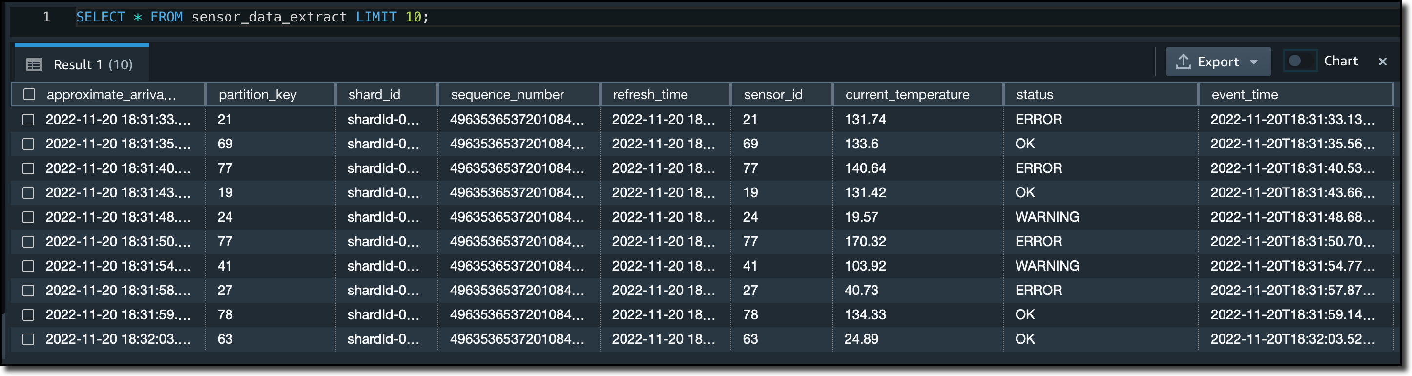
Cluster networking configuration

When you are ready, launch the instance. You are going to use the same instance to produce and consume messages. To do that, you need to set up Apache Kafka client tools in the instance. You can follow the Amazon MSK developer guide to get your instance ready.
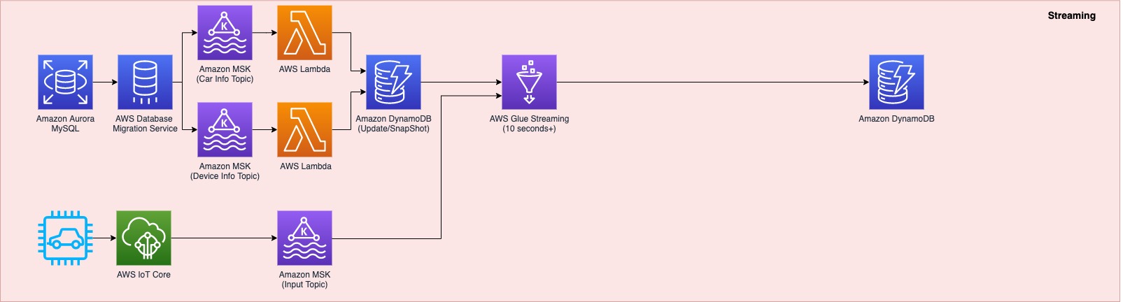
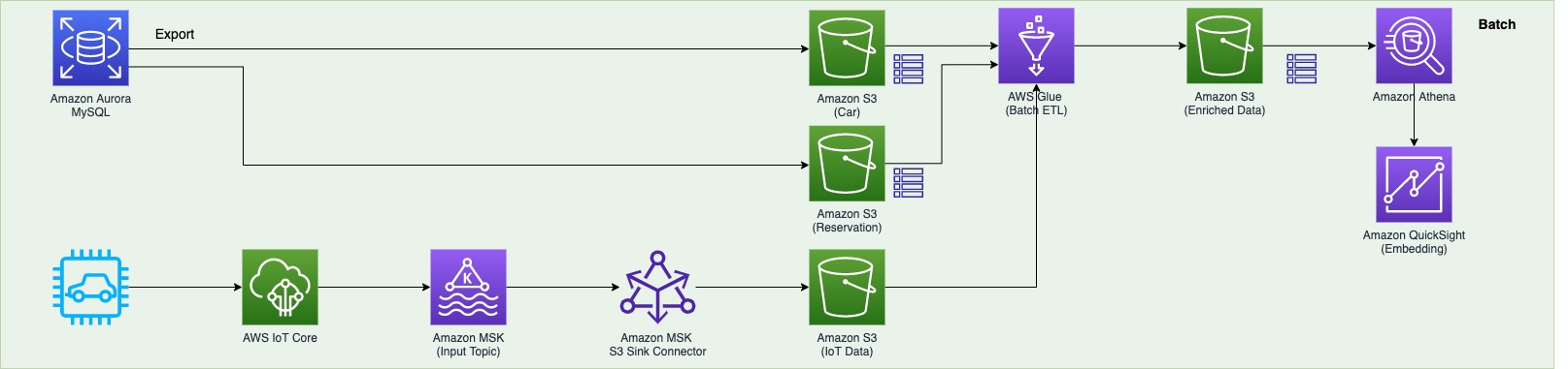
Producing and consuming records
Now that you have everything configured, you can start sending and receiving records using Amazon MSK Serverless. The first thing you need to do is to create a topic. From your EC2 instance, go to the directory where you installed the Apache Kafka tools and export the bootstrap server endpoint.

cd kafka_2.13-3.1.0/bin/
export BS=boot-abc1234.c3.kafka-serverless.us-east-2.amazonaws.com:9098

As you are using Amazon MSK Serverless, there is only one address for this server, and you can find it in the client information on your cluster page.

Viewing client information

Run the following command to create a topic with the name msk-serverless-tutorial.

./kafka-topics.sh --bootstrap-server $BS \
--command-config client.properties \
--create --topic msk-serverless-tutorial --partitions 6

Now you can start sending records. If you want to see the service work under a high throughput, you can use the Apache Kafka producer performance test tool. This tool allows you to send many messages at the same time to the MSK cluster with a defined throughput and specific size. Experiment with this performance test tool, change the number of messages per second and the record size and see how the cluster behaves and adapts its capacity.

./kafka-topics.sh --bootstrap-server $BS \
--command-config client.properties \
--create --topic msk-serverless-tutorial --partitions 6

Finally, if you want to receive the messages, open a new terminal, connect to the same EC2 instance, and use the Apache Kafka consumer tool to receive the messages.

cd kafka_2.13-3.1.0/bin/
export BS=boot-abc1234.c3.kafka-serverless.us-east-2.amazonaws.com:9098
./kafka-console-consumer.sh \
--bootstrap-server $BS \
--consumer.config client.properties \
--topic msk-serverless-tutorial --from-beginning

You can see how the cluster is doing on the monitoring page of the Amazon MSK Serverless cluster.

Cluster metrics page

Availability
Amazon MSK Serverless is available in US East (Ohio), US East (N. Virginia), US West (Oregon), Europe (Frankfurt), Europe (Ireland), Europe (Stockholm), Asia Pacific (Singapore), Asia Pacific (Sydney), and Asia Pacific (Tokyo).
Learn more about this service and its pricing on the Amazon MSK Serverless feature page.

Marcia