Post Syndicated from Bandana Das original https://aws.amazon.com/blogs/big-data/how-volkswagen-streamlined-access-to-data-across-multiple-data-lakes-using-amazon-datazone-part-1/
Over the years, organizations have invested in creating purpose-built, cloud-based data lakes that are siloed from one another. A major challenge is enabling cross-organization discovery and access to data across these multiple data lakes, each built on different technology stacks. A data mesh addresses these issues with four principles: domain-oriented decentralized data ownership and architecture, treating data as a product, providing self-serve data infrastructure as a platform, and implementing federated governance. Data mesh enables organizations to organize around data domains with a focus on delivering data as a product.
In 2019, Volkswagen AG (VW) and Amazon Web Services (AWS) formed a strategic partnership to co-develop the Digital Production Platform (DPP), aiming to enhance production and logistics efficiency by 30 percent while reducing production costs by the same margin. The DPP was developed to streamline access to data from shop-floor devices and manufacturing systems by handling integrations and providing standardized interfaces. However, as applications evolved on the platform, a significant challenge emerged: sharing data across applications stored in multiple isolated data lakes in Amazon Simple Storage Service (Amazon S3) buckets in individual AWS accounts without having to consolidate data into a central data lake. Another challenge is discovering available data stored across multiple data lakes and facilitating a workflow to request data access across business domains within each plant. The current method is largely manual, relying on emails and general communication, which not only increases overhead but also varies from one use case to another in terms of data governance. This blog post introduces Amazon DataZone and explores how VW used it to build their data mesh to enable streamlined data access across multiple data lakes. It focuses on the key aspect of the solution, which was enabling data providers to automatically publish data assets to Amazon DataZone, which served as the central data mesh for enhanced data discoverability. Additionally, the post provides code to guide you through the implementation.
Introduction to Amazon DataZone
Amazon DataZone is a data management service that makes it faster and easier for customers to catalog, discover, share, and govern data stored across AWS, on premises, and third-party sources. Key features of Amazon DataZone include a business data catalog that allows users to search for published data, request access, and start working on data in days instead of weeks. Amazon DataZone projects enable collaboration with teams through data assets and the ability to manage and monitor data assets across projects. It also includes the Amazon DataZone portal, which offers a personalized analytics experience for data assets through a web-based application or API. Lastly, Amazon DataZone governed data sharing ensures that the right data is accessed by the right user for the right purpose with a governed workflow.
Architecture for Data Management with Amazon DataZone
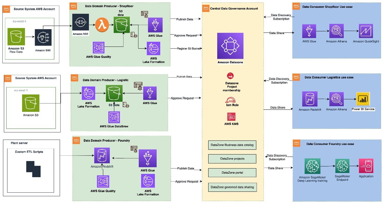
Figure 1: Data mesh pattern implementation on AWS using Amazon DataZone
The architecture diagram (Figure 1) represents a high-level design based on the data mesh pattern. It separates source systems, data domain producers (data publishers), data domain consumers (data subscribers), and central governance to highlight key aspects. This cross-account data mesh architecture aims to create a scalable foundation for data platforms, supporting producers and consumers with consistent governance.
- A data domain producer resides in an AWS account and uses Amazon S3 buckets to store raw and transformed data. Producers ingest data into their S3 buckets through pipelines they manage, own, and operate. They are responsible for the full lifecycle of the data, from raw capture to a form suitable for external consumption.
- A data domain producer maintains its own ETL stack using AWS Glue, AWS Lambda to process, AWS Glue Databrew to profile the data and prepare the data asset (data product) before cataloguing it into AWS Glue Data Catalog in their account.
- A second pattern could be that a data domain producer prepares and stores the data asset as table within Amazon Redshift using AWS S3 Copy.
- Data domain producers publish data assets using datasource run to Amazon DataZone in the Central Governance account. This populates the technical metadata in the business data catalog for each data asset. The business metadata, can be added by business users to provide business context, tags, and data classification for the datasets. Producers control what to share, for how long, and how consumers interact with it.
- Producers can register and create catalog entries with AWS Glue from all their S3 buckets. The central governance account securely shares datasets between producers and consumers via metadata linking, with no data (except logs) existing in this account. Data ownership remains with the producer.
- With Amazon DataZone, once data is cataloged and published into the DataZone domain, it can be shared with multiple consumer accounts.
- The Amazon DataZone Data portal provides a personalized view for users to discover/search and submit requests for subscription of data assets using a web-based application. The data domain producer receives the notification of subscription requests in the Data portal and can approve/reject the requests.
- Once approved, the consumer account can read and further process data assets to implement various use cases with AWS Lambda, AWS Glue, Amazon Athena, Amazon Redshift query editor v2, Amazon QuickSight (Analytics use cases) and with Amazon Sagemaker (Machine learning use cases).
Manual process to publish data assets to Amazon DataZone
To publish a data asset from the producer account, each asset must be registered in Amazon DataZone as a data source for consumer subscription. The Amazon DataZone User Guide provides detailed steps to achieve this. In the absence of an automated registration process, all required tasks must be completed manually for each data asset.
How to automate publishing data assets from AWS Glue Data Catalog from the producer account to Amazon DataZone
Using the automated registration workflow, the manual steps can be automated for any new data asset that needs to be published in an Amazon DataZone domain or when there’s a schema change in an already published data asset.
The automated solution reduces the repetitive manual steps to publish the data sources (AWS Glue tables) into an Amazon DataZone domain.
Architecture for automated data asset publish
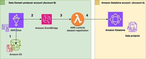
Figure 2 Architecture for automated data publish to Amazon DataZone
To automate publishing data assets:
- In the producer account (Account B), the data to be shared resides in an Amazon S3 bucket (Figure 2). An AWS Glue crawler is configured for the dataset to automatically create the schema using AWS Cloud Development Kit (AWS CDK).
- Once configured, the AWS Glue crawler crawls the Amazon S3 bucket and updates the metadata in the AWS Glue Data Catalog. The successful completion of the AWS Glue crawler generates an event in the default event bus of Amazon EventBridge.
- An EventBridge rule is configured to detect this event and invoke a dataset-registration AWS Lambda function.
- The AWS Lambda function performs all the steps to automatically register and publish the dataset in Amazon Datazone.
Steps performed in the dataset-registration AWS Lambda function
-
- The AWS Lambda function retrieves the AWS Glue database and Amazon S3 information for the dataset from the Amazon Eventbridge event triggered by the successful run of the AWS Glue crawler.
- It obtains the Amazon DataZone Datalake blueprint ID from the producer account and the Amazon DataZone domain ID and project ID by assuming an IAM role in the central governance account where the Amazon Datazone domain exists.
- It enables the Amazon DataZone Datalake blueprint in the producer account.
- It checks if the Amazon Datazone environment already exists within the Amazon DataZone project. If it does not, then it initiates the environment creation process. If the environment exists, it proceeds to the next step.
- It registers the Amazon S3 location of the dataset in Lake Formation in the producer account.
- The function creates a data source within the Amazon DataZone project and monitors the completion of the data source creation.
- Finally, it checks whether the data source sync job in Amazon DataZone needs to be started. If new AWS Glue tables or metadata is created or updated, then it starts the data source sync job.
Prerequisites
As part of this solution, you will publish data assets from an existing AWS Glue database in a producer account into an Amazon DataZone domain for which the following prerequisites need to be performed.
- You need two AWS accounts to deploy the solution.
- One AWS account will act as the data domain producer account (Account B) which will contain the AWS Glue dataset to be shared.
- The second AWS account is the central governance account (Account A), which will have the Amazon DataZone domain and project deployed. This is the Amazon DataZone account.
- Ensure that both the AWS accounts belong to the same AWS Organization
- Remove the IAMAllowedPrincipals permissions from the AWS Lake Formation tables for which Amazon DataZone handles permissions.
- Make sure in both AWS accounts that you have cleared the checkbox for Default permissions for newly created databases and tables under the Data Catalog settings in Lake Formation (Figure 3).

Figure 3: Clear default permissions in AWS Lake Formation
- Sign in to Account A (central governance account) and make sure you have created an Amazon DataZone domain and a project within the domain.
- If your Amazon DataZone domain is encrypted with an AWS Key Management Service (AWS KMS) key, add Account B (producer account) to the key policy with the following actions:
- Ensure you have created an AWS Identity and Access Management (IAM) role that Account B (producer account) can assume and this IAM role is added as a member (as contributor) of your Amazon DataZone project. The role should have the following permissions:
- This IAM role is called
dz-assumable-env-dataset-registration-rolein this example. Adding this role will enable you to successfully run thedataset-registrationLambda function. Replace theaccount-region,account id, andDataZonekmsKeyin the following policy with your information. These values correspond to where your Amazon DataZone domain is created and the AWS KMS key Amazon Resource Name (ARN) used to encrypt the Amazon DataZone domain. - Add the AWS account in the trust relationship of this role with the following trust relationship. Replace
ProducerAccountIdwith the AWS account ID of Account B (data domain producer account).
- This IAM role is called
- The following tools are needed to deploy the solution using AWS CDK:
- Either Bash or ZSH terminal
- Node and NPM using Node Version Manager
- Install Node Version Manager (NVM)
- Install Node version 18.12.0 using following command
-
-
- The node and npm binaries should now be available
- Python
- AWS Command Line Interface (AWS CLI)
- AWS SDK for Python
- AWS CDK
-
Deployment Steps
After completing the pre-requisites, use the AWS CDK stack provided on GitHub to deploy the solution for automatic registration of data assets into DataZone domain
- Clone the repository from GitHub to your preferred IDE using the following commands.
- At the base of the repository folder, run the following commands to build and deploy resources to AWS.
- Sign in to the AWS account B (the data domain producer account) using AWS Command Line Interface (AWS CLI) with your profile name.
- Ensure you have configured the AWS Region in your credential’s configuration file.
- Bootstrap the CDK environment with the following commands at the base of the repository folder. Replace
<PROFILE_NAME>with the profile name of your deployment account (Account B). Bootstrapping is a one-time activity and is not needed if your AWS account is already bootstrapped. - Replace the placeholder parameters (marked with the suffix
_PLACEHOLDER) in the fileconfig/DataZoneConfig.ts(Figure 4).
-
- Amazon DataZone domain and project name of your Amazon DataZone instance. Make sure all names are in lowercase.
- The AWS account ID and Region.
- The assumable IAM role from the prerequisites.
- The deployment role starting with
cfn-xxxxxx-cdk-exec-role-.
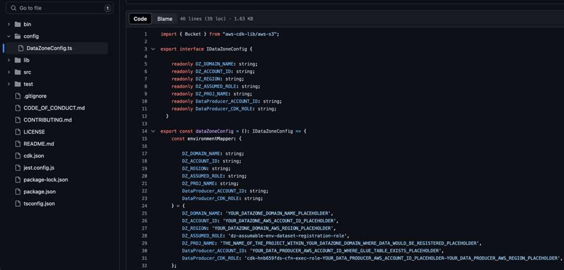
Figure 4: Edit the DataZoneConfig file
- In the AWS Management Console for Lake Formation, select Administrative roles and tasks from the navigation pane (Figure 5) and make sure the IAM role for AWS CDK deployment that starts with
cfn-xxxxxx-cdk-exec-role-is selected as an administrator in Data lake administrators. This IAM role needs permissions in Lake Formation to create resources, such as an AWS Glue database. Without these permissions, the AWS CDK stack deployment will fail.
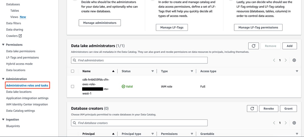
Figure 5: Add cfn-xxxxxx-cdk-exec-role- as a Data Lake administrator
- Use the following command in the base folder to deploy the AWS CDK solution
During deployment, enter y if you want to deploy the changes for some stacks when you see the prompt Do you wish to deploy these changes (y/n)?
- After the deployment is complete, sign in to your AWS account B (producer account) and navigate to the AWS CloudFormation console to verify that the infrastructure deployed. You should see a list of the deployed CloudFormation stacks as shown in Figure 6.
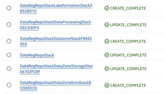
Figure 6: Deployed CloudFormation stacks
Test automatic data registration to Amazon DataZone
To test, we use the Online Retail Transactions dataset from Kaggle as a sample dataset to demonstrate the automatic data registration.
- Download the Online Retail.csv file from Kaggle dataset.
- Login to AWS Account B (producer account) and navigate to the Amazon S3 console, find the
DataZone-test-datasourceS3 bucket, and upload the csv file there (Figure 7).
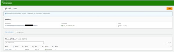
Figure 7: Upload the dataset CSV file
- The AWS Glue crawler is scheduled to run at a specific time each day. However for testing, you can manually run the crawler by going to the AWS Glue console and selecting Crawlers from the navigation pane. Run the on-demand crawler starting with
DataZone-. After the crawler has run, verify that a new table has been created. - Go to the Amazon DataZone console in AWS account A (central governance account) where you deployed the resources. Select Domains in the navigation pane (Figure 8), then Select and open your domain.

Figure 8: Amazon DataZone domains
- After you open the Datazone Domain, you can find the Amazon Datazone data portal URL in the Summary section (Figure 9). Select and open data portal.

Figure 9: Amazon DataZone data portal URL
- In the data portal find your project (Figure 10). Then select the Data tab at the top of the window.

Figure 10: Amazon DataZone Project overview
- Select the section Data Sources (Figure 11) and find the newly created data source DataZone-testdata-db.

Figure 11: Select Data sources in the Amazon Datazone Domain Data portal
- Verify that the data source has been successfully published (Figure 12).

Figure 12: The data sources are visible in the Published data section
- After the data sources are published, users can discover the published data and can submit a subscription request. The data producer can approve or reject requests. Upon approval, users can consume the data by querying data in Amazon Athena. Figure 13 illustrates data discovery in the Amazon DataZone data portal.

Figure 13: Example data discovery in the Amazon DataZone portal


Clean up
Use the following steps to clean up the resources deployed through the CDK.
- Empty the two S3 buckets that were created as part of this deployment.
- Go to the Amazon DataZone domain portal and delete the published data assets that were created in the Amazon DataZone project by the
dataset-registrationLambda function. - Delete the remaining resources created using the following command in the base folder:
Conclusion
By using AWS Glue and Amazon DataZone, organizations can make their data management easier and allow teams to share and collaborate on data smoothly. Automatically sending AWS Glue data to Amazon DataZone not only makes the process simple but also keeps the data consistent, secure, and well-governed. Simplify and standardize publishing data assets to Amazon DataZone and streamline data management with Amazon DataZone. For guidance on establishing your organization’s data mesh with Amazon DataZone, contact your AWS team today.
About the Authors
 Bandana Das is a Senior Data Architect at Amazon Web Services and specializes in data and analytics. She builds event-driven data architectures to support customers in data management and data-driven decision-making. She is also passionate about enabling customers on their data management journey to the cloud.
 Anirban Saha is a DevOps Architect at AWS, specializing in architecting and implementation of solutions for customer challenges in the automotive domain. He is passionate about well-architected infrastructures, automation, data-driven solutions and helping make the customer’s cloud journey as seamless as possible. Personally, he likes to keep himself engaged with reading, painting, language learning and traveling.
 Chandana Keswarkar is a Senior Solutions Architect at AWS, who specializes in guiding automotive customers through their digital transformation journeys by using cloud technology. She helps organizations develop and refine their platform and product architectures and make well-informed design decisions. In her free time, she enjoys traveling, reading, and practicing yoga.
 Sindi Cali is a ProServe Associate Consultant with AWS Professional Services. She supports customers in building data driven applications in AWS.

 Clarisa Tavolieri is a Software Engineering graduate with qualifications in Business, Audit, and Strategy Consulting. With an extensive career in the financial and tech industries, she specializes in data management and has been involved in initiatives ranging from reporting to data architecture. She currently serves as the Global Head of Cyber Data Management at Zurich Group. In her role, she leads the data strategy to support the protection of company assets and implements advanced analytics to enhance and monitor cybersecurity tools.
 Austin Rappeport is a Computer Engineer who graduated from the University of Illinois Urbana/Champaign in 2011 with a focus in Computer Security. After graduation, he worked for the Federal Energy Regulatory Commission in the Office of Electric Reliability, working with the North American Electric Reliability Corporation’s Critical Infrastructure Protection Standards on both the audit and enforcement side, as well as standards development. Austin currently works for Zurich Insurance as the Global Head of Detection Engineering and Automation, where he leads the team responsible for using Zurich’s security tools to detect suspicious and malicious activity and improve internal processes through automation.
 Samantha Gignac is a Global Security Architect at Zurich Insurance. She graduated from Ferris State University in 2014 with a Bachelor’s degree in Computer Systems & Network Engineering. With experience in the insurance, healthcare, and supply chain industries, she has held roles such as Storage Engineer, Risk Management Engineer, Vulnerability Management Engineer, and SOC Engineer. As a Cybersecurity Architect, she designs and implements secure network systems to protect organizational data and infrastructure from cyber threats.
 Claire Sheridan is a Principal Solutions Architect with Amazon Web Services working with global financial services customers. She holds a PhD in Informatics and has more than 15 years of industry experience in tech. She loves traveling and visiting art galleries.
 Jake Obi is a Principal Security Consultant with Amazon Web Services based in South Carolina, US, with over 20 years’ experience in information technology. He helps financial services customers improve their security posture in the cloud. Prior to joining Amazon, Jake was an Information Assurance Manager for the US Navy, where he worked on a large satellite communications program as well as hosting government websites using the public cloud.
 Srikanth Daggumalli is an Analytics Specialist Solutions Architect in AWS. Out of 18 years of experience, he has over a decade of experience in architecting cost-effective, performant, and secure enterprise applications that improve customer reachability and experience, using big data, AI/ML, cloud, and security technologies. He has built high-performing data platforms for major financial institutions, enabling improved customer reach and exceptional experiences. He is specialized in services like cross-border transactions and architecting robust analytics platforms.
 Freddy Kasprzykowski is a Senior Security Consultant with Amazon Web Services based in Florida, US, with over 20 years’ experience in information technology. He helps customers adopt AWS services securely according to industry best practices, standards, and compliance regulations. He is a member of the Customer Incident Response Team (CIRT), helping customers during security events, a seasoned speaker at AWS re:Invent and AWS re:Inforce conferences, and a contributor to open source projects related to AWS security.


 Chiho Sugimoto is a Cloud Support Engineer on the AWS Big Data Support team. She is passionate about helping customers build data lakes using ETL workloads. She loves planetary science and enjoys studying the asteroid Ryugu on weekends.
 Fabrizio Napolitano is a Principal Specialist Solutions Architect or Data Analytics at AWS. He has worked in the analytics domain for the last 20 years, now focusing on helping Canadian public sector organizations innovate with data. Quite by surprise, he become a Hockey Dad after moving to Canada.
 Noritaka Sekiyama is a Principal Big Data Architect on the AWS Glue team. He is responsible for building software artifacts to help customers. In his spare time, he enjoys cycling with his new road bike.
 Gal Heyne is a Technical Product Manager for AWS Data Processing services with a strong focus on AI/ML, data engineering, and BI. She is passionate about developing a deep understanding of customers’ business needs and collaborating with engineers to design easy-to-use data services products.


 Sotaro Hikita is a Solutions Architect. He supports customers in a wide range of industries, especially the financial industry, to build better solutions. He is particularly passionate about big data technologies and open source software.
 Noritaka Sekiyama is a Principal Big Data Architect on the AWS Glue team. He is responsible for building software artifacts to help customers. In his spare time, he enjoys cycling with his new road bike.
 Kyle Duong is a Senior Software Development Engineer on the AWS Glue and AWS Lake Formation team. He is passionate about building big data technologies and distributed systems.
 Kalaiselvi Kamaraj is a Senior Software Development Engineer with Amazon. She has worked on several projects within the Amazon Redshift query processing team and currently focusing on performance-related projects for Redshift data lakes.
 Sandeep Adwankar is a Senior Product Manager at AWS. Based in the California Bay Area, he works with customers around the globe to translate business and technical requirements into products that enable customers to improve how they manage, secure, and access data.


 Gonzalo Herreros is a Senior Big Data Architect on the AWS Glue team, with a background in machine learning and AI.
 Keerthi Chadalavada is a Senior Software Development Engineer at AWS Glue. She is passionate about designing and building end-to-end solutions to address customer data integration and analytic needs.


 Yonatan Dolan is a Principal Analytics Specialist at Amazon Web Services. He is located in Israel and helps customers harness AWS analytical services to leverage data, gain insights, and derive value. Yonatan is an Apache Iceberg evangelist.
 Amit Gilad is a Senior Data Engineer on the Data Infrastructure team at Cloudinar. He is currently leading the strategic transition from traditional data warehouses to a modern data lakehouse architecture, utilizing Apache Iceberg to enhance scalability and flexibility.
 Alex Dickman is a Staff Data Engineer on the Data Infrastructure team at Cloudinary. He focuses on engaging with various internal teams to consolidate the team’s data infrastructure and create new opportunities for data applications, ensuring robust and scalable data solutions for Cloudinary’s diverse requirements.
 Itay Takersman is a Senior Data Engineer at Cloudinary data infrastructure team. Focused on building resilient data flows and aggregation pipelines to support Cloudinary’s data requirements.


 Sudipta Mitra is a Senior Data Architect for AWS, and passionate about helping customers to build modern data analytics applications by making innovative use of latest AWS services and their constantly evolving features. A pragmatic architect who works backwards from customer needs, making them comfortable with the proposed solution, helping achieve tangible business outcomes. His main areas of work are Data Mesh, Data Lake, Knowledge Graph, Data Security and Data Governance.
 Deepak Sharma is a Senior Data Architect with the AWS Professional Services team, specializing in big data and analytics solutions. With extensive experience in designing and implementing scalable data architectures, he collaborates closely with enterprise customers to build robust data lakes and advanced analytical applications on the AWS platform.
 Nanda Chinnappa is a Cloud Infrastructure Architect with AWS Professional Services at Amazon Web Services. Nanda specializes in Infrastructure Automation, Cloud Migration, Disaster Recovery and Databases which includes Amazon RDS and Amazon Aurora. He helps AWS Customer’s adopt AWS Cloud and realize their business outcome by executing cloud computing initiatives.


 Prasad Nadig is an Analytics Specialist Solutions Architect at AWS. He guides customers architect optimal data and analytical platforms leveraging the scalability and agility of the cloud. He is passionate about understanding emerging challenges and guiding customers to build modern solutions. Outside of work, Prasad indulges his creative curiosity through photography, while also staying up-to-date on the latest technology innovations and trends.
 Tyler McDaniel is a software development engineer on the AWS Glue team with diverse technical interests including high-performance computing and optimization, distributed systems, and machine learning operations. He has eight years of experience in software and research roles.
 Rahul Sharma is a Senior Software Development Engineer at AWS Glue. He focuses on building distributed systems to support features in AWS Glue. He has a passion for helping customers build data management solutions on the AWS Cloud. In his spare time, he enjoys playing the piano and gardening.
 Edward Cho is a Software Development Engineer at AWS Glue. He has contributed to the AWS Glue Data Quality feature as well as the underlying open-source project Deequ.

 Emilio Garcia Montano is a Solutions Architect at Amazon Web Services. He works with media and entertainment customers and supports them to achieve their outcomes with machine learning and AI.
 Carlos Rodrigues is a Big Data Specialist Solutions Architect at AWS. He helps customers worldwide build transactional data lakes on AWS using open table formats like Apache Iceberg and Apache Hudi. He can be reached via
  Imtiaz (Taz) Sayed is the WW Tech Leader for Analytics at AWS. He is an expert on data engineering and enjoys engaging with the community on all things data and analytics. He can be reached via
  Shana Schipers is an Analytics Specialist Solutions Architect at AWS, focusing on big data. She supports customers worldwide in building transactional data lakes using open table formats like Apache Hudi, Apache Iceberg, and Delta Lake on AWS.


 Leonardo Gomez is a Principal Analytics Specialist Solutions Architect at AWS. He has over a decade of experience in data management, helping customers around the globe address their business and technical needs. Connect with him on
  Michael Chess – is a Product Manager on the AWS Lake Formation team based out of Palo Alto, CA. He specializes in permissions and data catalog features in the data lake.
 Derek Liu – is a Senior Solutions Architect based out of Vancouver, BC. He enjoys helping customers solve big data challenges through AWS analytic services.


 Salim Tutuncu is a Sr. PSA Specialist on Data & AI, based from Amsterdam with a focus on the EMEA North and EMEA Central regions. With a rich background in the technology sector that spans roles as a Data Engineer, Data Scientist, and Machine Learning Engineer, Salim has built a formidable expertise in navigating the complex landscape of data and artificial intelligence. His current role involves working closely with partners to develop long-term, profitable businesses leveraging the AWS Platform, particularly in Data and AI use cases.
 Angel Conde Manjon is a Sr. PSA Specialist on Data & AI, based in Madrid, and focuses on EMEA South and Israel. He has previously worked on research related to Data Analytics and Artificial Intelligence in diverse European research projects. In his current role, Angel helps partners develop businesses centered on Data and AI.


 Junpei Ozono is a Go-to-market Data & AI solutions architect at AWS in Japan. Junpei supports customers’ journeys on the AWS Cloud from Data & AI aspects and guides them to design and develop data-driven architectures powered by AWS services.


 Vishal Kajjam is a Software Development Engineer on the AWS Glue team. He is passionate about distributed computing and using ML/AI for designing and building end-to-end solutions to address customers’ data integration needs. In his spare time, he enjoys spending time with family and friends.


 Sidhanth Muralidhar is a Principal Technical Account Manager at AWS. He works with large enterprise customers who run their workloads on AWS. He is passionate about working with customers and helping them architect workloads for costs, reliability, performance, and operational excellence at scale in their cloud journey. He has a keen interest in data analytics as well.


 Takeshi Nakatani is a Principal Big Data Consultant on the Professional Services team in Tokyo. He has 26 years of experience in the IT industry, with expertise in architecting data infrastructure. On his days off, he can be a rock drummer or a motorcyclist.

 Atul Khare is a Director of Engineering at Salesforce Security, where he spearheads the Security Log Platform and Data Lakehouse initiatives. He supports diverse security customers by building robust big data ETL pipeline that is elastic, resilient, and easy to use, providing uniform & consistent security datasets for threat detection and response operations, AI, forensic analysis, analytics, and compliance needs across all Salesforce clouds. Beyond his professional endeavors, Atul enjoys performing music with his band to raise funds for local charities.
 Bhupender Panwar is a Big Data Architect at Salesforce and seasoned advocate for big data and cloud computing. His background encompasses the development of data-intensive applications and pipelines, solving intricate architectural and scalability challenges, and extracting valuable insights from extensive datasets within the technology industry. Outside of his big data work, Bhupender loves to hike, bike, enjoy travel and is a great foodie.
 Avijit Goswami is a Principal Solutions Architect at AWS specialized in data and analytics. He supports AWS strategic customers in building high-performing, secure, and scalable data lake solutions on AWS using AWS managed services and open-source solutions. Outside of his work, Avijit likes to travel, hike in the San Francisco Bay Area trails, watch sports, and listen to music.
 Vikas Panghal is the Principal Product Manager leading the product management team for Amazon SNS and Amazon SQS. He has deep expertise in event-driven and messaging applications and brings a wealth of knowledge and experience to his role, shaping the future of messaging services. He is passionate about helping customers build highly scalable, fault-tolerant, and loosely coupled systems. Outside of work, he enjoys spending time with his family outdoors, playing chess, and running.


 Utkarsh Mittal is a Senior Technical Product Manager for Amazon DataZone at AWS. He is passionate about building innovative products that simplify customers’ end-to-end analytics journeys. Outside of the tech world, Utkarsh loves to play music, with drums being his latest endeavor.
 Praveen Kumar is a Principal Analytics Solution Architect at AWS with expertise in designing, building, and implementing modern data and analytics platforms using cloud-centered services. His areas of interests are serverless technology, modern cloud data warehouses, streaming, and generative AI applications.
 Paul Villena is a Senior Analytics Solutions Architect in AWS with expertise in building modern data and analytics solutions to drive business value. He works with customers to help them harness the power of the cloud. His areas of interests are infrastructure as code, serverless technologies, and coding in Python


 Andrea Filippo is a Partner Solutions Architect at AWS supporting Public Sector partners and customers in Italy. He focuses on modern data architectures and helping customers accelerate their cloud journey with serverless technologies.
 Emanuele is a Solutions Architect at AWS, based in Italy, after living and working for more than 5 years in Spain. He enjoys helping large companies with the adoption of cloud technologies, and his area of expertise is mainly focused on Data Analytics and Data Management. Outside of work, he enjoys traveling and collecting action figures.
 Varsha Velagapudi is a Senior Technical Product Manager with Amazon DataZone at AWS. She focuses on improving data discovery and curation required for data analytics. She is passionate about simplifying customers’ AI/ML and analytics journey to help them succeed in their day-to-day tasks. Outside of work, she enjoys nature and outdoor activities, reading, and traveling.