Tag Archives: AWS Glue

Simplify data loading into Type 2 slowly changing dimensions in Amazon Redshift

Post Syndicated from Vaidy Kalpathy original https://aws.amazon.com/blogs/big-data/simplify-data-loading-into-type-2-slowly-changing-dimensions-in-amazon-redshift/

Thousands of customers rely on Amazon Redshift to build data warehouses to accelerate time to insights with fast, simple, and secure analytics at scale and analyze data from terabytes to petabytes by running complex analytical queries. Organizations create data marts, which are subsets of the data warehouse and usually oriented for gaining analytical insights specific to a business unit or team. The star schema is a popular data model for building data marts.

In this post, we show how to simplify data loading into a Type 2 slowly changing dimension in Amazon Redshift.

Star schema and slowly changing dimension overview

A star schema is the simplest type of dimensional model, in which the center of the star can have one fact table and a number of associated dimension tables. A dimension is a structure that captures reference data along with associated hierarchies, while a fact table captures different values and metrics that can be aggregated by dimensions. Dimensions provide answers to exploratory business questions by allowing end-users to slice and dice data in a variety of ways using familiar SQL commands.

Whereas operational source systems contain only the latest version of master data, the star schema enables time travel queries to reproduce dimension attribute values on past dates when the fact transaction or event actually happened. The star schema data model allows analytical users to query historical data tying metrics to corresponding dimensional attribute values over time. Time travel is possible because dimension tables contain the exact version of the associated attributes at different time ranges. Relative to the metrics data that keeps changing on a daily or even hourly basis, the dimension attributes change less frequently. Therefore, dimensions in a star schema that keeps track of changes over time are referred to as slowly changing dimensions (SCDs).

Data loading is one of the key aspects of maintaining a data warehouse. In a star schema data model, the central fact table is dependent on the surrounding dimension tables. This is captured in the form of primary key-foreign key relationships, where the dimension table primary keys are referred by foreign keys in the fact table. In the case of Amazon Redshift, uniqueness, primary key, and foreign key constraints are not enforced. However, declaring them will help the optimizer arrive at optimal query plans, provided that the data loading processes enforce their integrity. As part of data loading, the dimension tables, including SCD tables, get loaded first, followed by the fact tables.

SCD population challenge

Populating an SCD dimension table involves merging data from multiple source tables, which are usually normalized. SCD tables contain a pair of date columns (effective and expiry dates) that represent the record’s validity date range. Changes are inserted as new active records effective from the date of data loading, while simultaneously expiring the current active record on a previous day. During each data load, incoming change records are matched against existing active records, comparing each attribute value to determine whether existing records have changed or were deleted or are new records coming in.

In this post, we demonstrate how to simplify data loading into a dimension table with the following methods:

  • Using Amazon Simple Storage Service (Amazon S3) to host the initial and incremental data files from source system tables
  • Accessing S3 objects using Amazon Redshift Spectrum to carry out data processing to load native tables within Amazon Redshift
  • Creating views with window functions to replicate the source system version of each table within Amazon Redshift
  • Joining source table views to project attributes matching with dimension table schema
  • Applying incremental data to the dimension table, bringing it up to date with source-side changes

Solution overview

In a real-world scenario, records from source system tables are ingested on a periodic basis to an Amazon S3 location before being loaded into star schema tables in Amazon Redshift.

For this demonstration, data from two source tables, customer_master and customer_address, are combined to populate the target dimension table dim_customer, which is the customer dimension table.

The source tables customer_master and customer_address share the same primary key, customer_id, and will be joined on the same to fetch one record per customer_id along with attributes from both tables. row_audit_ts contains the latest timestamp at which the particular source record was inserted or last updated. This column helps identify the change records since the last data extraction.

rec_source_status is an optional column that indicates if the corresponding source record was inserted, updated, or deleted. This is applicable in cases where the source system itself provides the changes and populates rec_source_status appropriately.

The following figure provides the schema of the source and target tables.

Let’s look closer at the schema of the target table, dim_customer. It contains different categories of columns:

  • Keys – It contains two types of keys:
    • customer_sk is the primary key of this table. It is also called the surrogate key and has a unique value that is monotonically increasing.
    • customer_id is the source primary key and provides a reference back to the source system record.
  • SCD2 metadatarec_eff_dt and rec_exp_dt indicate the state of the record. These two columns together define the validity of the record. The value in rec_exp_dt will be set as ‘9999-12-31’ for presently active records.
  • Attributes – Includes first_name, last_name, employer_name, email_id, city, and country.

Data loading into a SCD table involves a first-time bulk data loading, referred to as the initial data load. This is followed by continuous or regular data loading, referred to as an incremental data load, to keep the records up to date with changes in the source tables.

To demonstrate the solution, we walk through the following steps for initial data load (1–7) and incremental data load (8–12):

  1. Land the source data files in an Amazon S3 location, using one subfolder per source table.
  2. Use an AWS Glue crawler to parse the data files and register tables in the AWS Glue Data Catalog.
  3. Create an external schema in Amazon Redshift to point to the AWS Glue database containing these tables.
  4. In Amazon Redshift, create one view per source table to fetch the latest version of the record for each primary key (customer_id) value.
  5. Create the dim_customer table in Amazon Redshift, which contains attributes from all relevant source tables.
  6. Create a view in Amazon Redshift joining the source table views from Step 4 to project the attributes modeled in the dimension table.
  7. Populate the initial data from the view created in Step 6 into the dim_customer table, generating customer_sk.
  8. Land the incremental data files for each source table in their respective Amazon S3 location.
  9. In Amazon Redshift, create a temporary table to accommodate the change-only records.
  10. Join the view from Step 6 and dim_customer and identify change records comparing the combined hash value of attributes. Populate the change records into the temporary table with an I, U, or D indicator.
  11. Update rec_exp_dt in dim_customer for all U and D records from the temporary table.
  12. Insert records into dim_customer, querying all I and U records from the temporary table.

Prerequisites

Before you get started, make sure you meet the following prerequisites:

Land data from source tables

Create separate subfolders for each source table in an S3 bucket and place the initial data files within the respective subfolder. In the following image, the initial data files for customer_master and customer_address are made available within two different subfolders. To try out the solution, you can use customer_master_with_ts.csv and customer_address_with_ts.csv as initial data files.

It’s important to include an audit timestamp (row_audit_ts) column that indicates when each record was inserted or last updated. As part of incremental data loading, rows with the same primary key value (customer_id) can arrive more than once. The row_audit_ts column helps identify the latest version of such records for a given customer_id to be used for further processing.

Register source tables in the AWS Glue Data Catalog

We use an AWS Glue crawler to infer metadata from delimited data files like the CSV files used in this post. For instructions on getting started with an AWS Glue crawler, refer to Tutorial: Adding an AWS Glue crawler.

Create an AWS Glue crawler and point it to the Amazon S3 location that contains the source table subfolders, within which the associated data files are placed. When you’re creating the AWS Glue crawler, create a new database named rs-dimension-blog. The following screenshots show the AWS Glue crawler configuration chosen for our data files.

Note that for the Set output and scheduling section, the advanced options are left unchanged.

Running this crawler should create the following tables within the rs-dimension-blog database:

  • customer_address
  • customer_master

Create schemas in Amazon Redshift

First, create an AWS Identity and Access Management (IAM) role named rs-dim-blog-spectrum-role. For instructions, refer to Create an IAM role for Amazon Redshift.

The IAM role has Amazon Redshift as the trusted entity, and the permissions policy includes AmazonS3ReadOnlyAccess and AWSGlueConsoleFullAccess, because we’re using the AWS Glue Data Catalog. Then associate the IAM role with the Amazon Redshift cluster or endpoint.

Instead, you can also set the IAM role as the default for your Amazon Redshift cluster or endpoint. If you do so, in the following create external schema command, pass the iam_role parameter as iam_role default.

Now, open Amazon Redshift Query Editor V2 and create an external schema passing the newly created IAM role and specifying the database as rs-dimension-blog. The database name rs-dimension-blog is the one created in the Data Catalog as part of configuring the crawler in the preceding section. See the following code:

create external schema spectrum_dim_blog 
from data catalog 
database 'rs-dimension-blog' 
iam_role 'arn:aws:iam::<accountid>:role/rs-dim-blog-spectrum-role';

Check if the tables registered in the Data Catalog in the preceding section are visible from within Amazon Redshift:

select * 
from spectrum_dim_blog.customer_master 
limit 10;

select * 
from spectrum_dim_blog.customer_address 
limit 10;

Each of these queries will return 10 rows from the respective Data Catalog tables.

Create another schema in Amazon Redshift to host the table, dim_customer:

create schema rs_dim_blog;

Create views to fetch the latest records from each source table

Create a view for the customer_master table, naming it vw_cust_mstr_latest:

create view rs_dim_blog.vw_cust_mstr_latest as with rows_numbered as (
  select 
    customer_id, 
    first_name, 
    last_name, 
    employer_name, 
    row_audit_ts, 
    row_number() over(
      partition by customer_id 
      order by 
        row_audit_ts desc
    ) as rnum 
  from 
    spectrum_dim_blog.customer_master
) 
select 
  customer_id, 
  first_name, 
  last_name, 
  employer_name, 
  row_audit_ts, 
  rnum 
from 
  rows_numbered 
where 
  rnum = 1 with no schema binding;

The preceding query uses row_number, which is a window function provided by Amazon Redshift. Using window functions enables you to create analytic business queries more efficiently. Window functions operate on a partition of a result set, and return a value for every row in that window. The row_number window function determines the ordinal number of the current row within a group of rows, counting from 1, based on the ORDER BY expression in the OVER clause. By including the PARTITION BY clause as customer_id, groups are created for each value of customer_id and ordinal numbers are reset for each group.

Create a view for the customer_address table, naming it vw_cust_addr_latest:

create view rs_dim_blog.vw_cust_addr_latest as with rows_numbered as (
  select 
    customer_id, 
    email_id, 
    city, 
    country, 
    row_audit_ts, 
    row_number() over(
      partition by customer_id 
      order by 
        row_audit_ts desc
    ) as rnum 
  from 
    spectrum_dim_blog.customer_address
) 
select 
  customer_id, 
  email_id, 
  city, 
  country, 
  row_audit_ts, 
  rnum 
from 
  rows_numbered 
where 
  rnum = 1 with no schema binding;

Both view definitions use the row_number window function of Amazon Redshift, ordering the records by descending order of the row_audit_ts column (the audit timestamp column). The condition rnum=1 fetches the latest record for each customer_id value.

Create the dim_customer table in Amazon Redshift

Create dim_customer as an internal table in Amazon Redshift within the rs_dim_blog schema. The dimension table includes the column customer_sk, that acts as the surrogate key column and enables us to capture a time-sensitive version of each customer record. The validity period for each record is defined by the columns rec_eff_dt and rec_exp_dt, representing record effective date and record expiry date, respectively. See the following code:

create table rs_dim_blog.dim_customer (
  customer_sk bigint, 
  customer_id bigint, 
  first_name varchar(100), 
  last_name varchar(100), 
  employer_name varchar(100), 
  email_id varchar(100), 
  city varchar(100), 
  country varchar(100), 
  rec_eff_dt date, 
  rec_exp_dt date
) diststyle auto;

Create a view to consolidate the latest version of source records

Create the view vw_dim_customer_src, which consolidates the latest records from both source tables using left outer join, keeping them ready to be populated into the Amazon Redshift dimension table. This view fetches data from the latest views defined in the section “Create views to fetch the latest records from each source table”:

create view rs_dim_blog.vw_dim_customer_src as 
select 
  m.customer_id, 
  m.first_name, 
  m.last_name, 
  m.employer_name, 
  a.email_id, 
  a.city, 
  a.country 
from 
  rs_dim_blog.vw_cust_mstr_latest as m 
  left join rs_dim_blog.vw_cust_addr_latest as a on m.customer_id = a.customer_id 
order by 
  m.customer_id with no schema binding;

At this point, this view fetches the initial data for loading into the dim_customer table that we are about to create. In your use-case, use a similar approach to create and join the required source table views to populate your target dimension table.

Populate initial data into dim_customer

Populate the initial data into the dim_customer table by querying the view vw_dim_customer_src. Because this is the initial data load, running row numbers generated by the row_number window function will suffice to populate a unique value in the customer_sk column starting from 1:

insert into rs_dim_blog.dim_customer 
select 
  row_number() over() as customer_sk, 
  customer_id, 
  first_name, 
  last_name, 
  employer_name, 
  email_id, 
  city, 
  country, 
  cast('2022-07-01' as date) rec_eff_dt, 
  cast('9999-12-31' as date) rec_exp_dt 
from 
  rs_dim_blog.vw_dim_customer_src;

In this query, we have specified ’2022-07-01’ as the value in rec_eff_dt for all initial data records. For your use-case, you can modify this date value as appropriate to your situation.

The preceding steps complete the initial data loading into the dim_customer table. In the next steps, we proceed with populating incremental data.

Land ongoing change data files in Amazon S3

After the initial load, the source systems provide data files on an ongoing basis, either containing only new and change records or a full extract containing all records for a particular table.

You can use the sample files customer_master_with_ts_incr.csv and customer_address_with_ts_incr.csv, which contain changed as well as new records. These incremental files need to be placed in the same location in Amazon S3 where the initial data files were placed. Please see section “Land data from source tables”. This will result in the corresponding Redshift Spectrum tables automatically reading the additional rows.

If you used the sample file for customer_master, after adding the incremental files, the following query shows the initial as well as incremental records:

select 
  customer_id, 
  first_name, 
  last_name, 
  employer_name, 
  row_audit_ts 
from 
  spectrum_dim_blog.customer_master 
order by 
  customer_id;

In case of full extracts, we can identify deletes occurring in the source system tables by comparing the previous and current versions and looking for missing records. In case of change-only extracts where the rec_source_status column is present, its value will help us identify deleted records. In either case, land the ongoing change data files in the respective Amazon S3 locations.

For this example, we have uploaded the incremental data for the customer_master and customer_address source tables with a few customer_id records receiving updates and a few new records being added.

Create a temporary table to capture change records

Create the temporary table temp_dim_customer to store all changes that need to be applied to the target dim_customer table:

create temp table temp_dim_customer (
  customer_sk bigint, 
  customer_id bigint, 
  first_name varchar(100), 
  last_name varchar(100), 
  employer_name varchar(100), 
  email_id varchar(100), 
  city varchar(100), 
  country varchar(100), 
  rec_eff_dt date, 
  rec_exp_dt date, 
  iud_operation character(1)
);

Populate the temporary table with new and changed records

This is a multi-step process that can be combined into a single complex SQL. Complete the following steps:

  1. Fetch the latest version of all customer attributes by querying the view vw_dim_customer_src:
select 
  customer_id, 
  sha2(
    coalesce(first_name, '') || coalesce(last_name, '') || coalesce(employer_name, '') || coalesce(email_id, '') || coalesce(city, '') || coalesce(country, ''), 512
  ) as hash_value, 
  first_name, 
  last_name, 
  employer_name, 
  email_id, 
  city, 
  country, 
  current_date rec_eff_dt, 
  cast('9999-12-31' as date) rec_exp_dt 
from 
  rs_dim_blog.vw_dim_customer_src;

Amazon Redshift offers hashing functions such as sha2, which converts a variable length string input into a fixed length character output. The output string is a text representation of the hexadecimal value of the checksum with the specified number of bits. In this case, we pass a concatenated set of customer attributes whose change we want to track, specifying the number of bits as 512. We’ll use the output of the hash function to determine if any of the attributes have undergone a change. This dataset will be called newver (new version).

Because we landed the ongoing change data in the same location as the initial data files, the records retrieved from the preceding query (in newver) include all records, even the unchanged ones. But because of the definition of the view vw_dim_customer_src, we get only one record per customerid, which is its latest version based on row_audit_ts.

  1. In a similar manner, retrieve the latest version of all customer records from dim_customer, which are identified by rec_exp_dt=‘9999-12-31’. While doing so, also retrieve the sha2 value of all customer attributes available in dim_customer:
select 
  customer_id, 
  sha2(
    coalesce(first_name, '') || coalesce(last_name, '') || coalesce(employer_name, '') || coalesce(email_id, '') || coalesce(city, '') || coalesce(country, ''), 512
  ) as hash_value, 
  first_name, 
  last_name, 
  employer_name, 
  email_id, 
  city, 
  country 
from 
  rs_dim_blog.dim_customer 
where 
  rec_exp_dt = '9999-12-31';

This dataset will be called oldver (old or existing version).

  1. Identify the current maximum surrogate key value from the dim_customer table:
select 
  max(customer_sk) as maxval 
from 
  rs_dim_blog.dim_customer;

This value (maxval) will be added to the row_number before being used as the customer_sk value for the change records that need to be inserted.

  1. Perform a full outer join of the old version of records (oldver) and the new version (newver) of records on the customer_id column. Then compare the old and new hash values generated by the sha2 function to determine if the change record is an insert, update, or delete:
case when oldver.customer_id is null then 'I'
when newver.customer_id is null then 'D'
when oldver.hash_value != newver.hash_value then 'U'
else 'N' end as iud_op

We tag the records as follows:

  • If the customer_id is non-existent in the oldver dataset (oldver.customer_id is null), it’s tagged as an insert (‘I').
  • Otherwise, if the customer_id is non-existent in the newver dataset (newver.customer_id is null), it’s tagged as a delete (‘D').
  • Otherwise, if the old hash_value and new hash_value are different, these records represent an update (‘U').
  • Otherwise, it indicates that the record has not undergone any change and therefore can be ignored or marked as not-to-be-processed (‘N').

Make sure to modify the preceding logic if the source extract contains rec_source_status to identify deleted records.

Although sha2 output maps a possibly infinite set of input strings to a finite set of output strings, the chances of collision of hash values for the original row values and changed row values are very unlikely. Instead of individually comparing each column value before and after, we compare the hash values generated by sha2 to conclude if there has been a change in any of the attributes of the customer record. For your use-case, we recommend you choose a hash function that works for your data conditions after adequate testing. Instead, you can compare individual column values if none of the hash functions satisfactorily meet your expectations.

  1. Combining the outputs from the preceding steps, let’s create the INSERT statement that captures only change records to populate the temporary table:
insert into temp_dim_customer (
  customer_sk, customer_id, first_name, 
  last_name, employer_name, email_id, 
  city, country, rec_eff_dt, rec_exp_dt, 
  iud_operation
) with newver as (
  select 
    customer_id, 
    sha2(
      coalesce(first_name, '') || coalesce(last_name, '') || coalesce(employer_name, '') || coalesce(email_id, '') || coalesce(city, '') || coalesce(country, ''), 512
    ) as hash_value, 
    first_name, 
    last_name, 
    employer_name, 
    email_id, 
    city, 
    country, 
    current_date rec_eff_dt, 
    cast('9999-12-31' as date) rec_exp_dt 
  from 
    rs_dim_blog.vw_dim_customer_src
), 
oldver as (
  select 
    customer_id, 
    sha2(
      coalesce(first_name, '') || coalesce(last_name, '') || coalesce(employer_name, '') || coalesce(email_id, '') || coalesce(city, '') || coalesce(country, ''), 512
    ) as hash_value, 
    first_name, 
    last_name, 
    employer_name, 
    email_id, 
    city, 
    country 
  from 
    rs_dim_blog.dim_customer 
  where 
    rec_exp_dt = '9999-12-31'
), 
maxsk as (
  select 
    max(customer_sk) as maxval 
  from 
    rs_dim_blog.dim_customer
), 
allrecs as (
  select 
    coalesce(oldver.customer_id, newver.customer_id) as customer_id, 
    case when oldver.customer_id is null then 'I' when newver.customer_id is null then 'D' when oldver.hash_value != newver.hash_value then 'U' else 'N' end as iud_op, 
    newver.first_name, 
    newver.last_name, 
    newver.employer_name, 
    newver.email_id, 
    newver.city, 
    newver.country, 
    newver.rec_eff_dt, 
    newver.rec_exp_dt 
  from 
    oldver full 
    outer join newver on oldver.customer_id = newver.customer_id
) 
select 
  (maxval + (row_number() over())) as customer_sk, 
  customer_id, 
  first_name, 
  last_name, 
  employer_name, 
  email_id, 
  city, 
  country, 
  rec_eff_dt, 
  rec_exp_dt, 
  iud_op 
from 
  allrecs, 
  maxsk 
where 
  iud_op != 'N';

Expire updated customer records

With the temp_dim_customer table now containing only the change records (either ‘I’, ‘U’, or ‘D’), the same can be applied on the target dim_customer table.

Let’s first fetch all records with values ‘U’ or ‘D’ in the iud_op column. These are records that have either been deleted or updated in the source system. Because dim_customer is a slowly changing dimension, it needs to reflect the validity period of each customer record. In this case, we expire the presently active recorts that have been updated or deleted. We expire these records as of yesterday (by setting rec_exp_dt=current_date-1) matching on the customer_id column:

update 
  rs_dim_blog.dim_customer 
set 
  rec_exp_dt = current_date - 1 
where 
  customer_id in (
    select 
      customer_id 
    from 
      temp_dim_customer as t 
    where 
      iud_operation in ('U', 'D')
  ) 
  and rec_exp_dt = '9999-12-31';

Insert new and changed records

As the last step, we need to insert the newer version of updated records along with all first-time inserts. These are indicated by ‘U’ and ‘I’, respectively, in the iud_op column in the temp_dim_customer table:

insert into rs_dim_blog.dim_customer (
  customer_sk, customer_id, first_name, 
  last_name, employer_name, email_id, 
  city, country, rec_eff_dt, rec_exp_dt
) 
select 
  customer_sk, 
  customer_id, 
  first_name, 
  last_name, 
  employer_name, 
  email_id, 
  city, 
  country, 
  rec_eff_dt, 
  rec_exp_dt 
from 
  temp_dim_customer 
where 
  iud_operation in ('I', 'U');

Depending on the SQL client setting, you might want to run a commit transaction; command to verify that the preceding changes are persisted successfully in Amazon Redshift.

Check the final output

You can run the following query and see that the dim_customer table now contains both the initial data records plus the incremental data records, capturing multiple versions for those customer_id values that got changed as part of incremental data loading. The output also indicates that each record has been populated with appropriate values in rec_eff_dt and rec_exp_dt corresponding to the record validity period.

select 
  * 
from 
  rs_dim_blog.dim_customer 
order by 
  customer_id, 
  customer_sk;

For the sample data files provided in this article, the preceding query returns the following records. If you’re using the sample data files provided in this post, note that the values in customer_sk may not match with what is shown in the following table.

In this post, we only show the important SQL statements; the complete SQL code is available in load_scd2_sample_dim_customer.sql.

Clean up

If you no longer need the resources you created, you can delete them to prevent incurring additional charges.

Conclusion

In this post, you learned how to simplify data loading into Type-2 SCD tables in Amazon Redshift, covering both initial data loading and incremental data loading. The approach deals with multiple source tables populating a target dimension table, capturing the latest version of source records as of each run.

Refer to Amazon Redshift data loading best practices for further materials and additional best practices, and see Updating and inserting new data for instructions to implement updates and inserts.


About the Author

Vaidy Kalpathy is a Senior Data Lab Solution Architect at AWS, where he helps customers modernize their data platform and defines end to end data strategy including data ingestion, transformation, security, visualization. He is passionate about working backwards from business use cases, creating scalable and custom fit architectures to help customers innovate using data analytics services on AWS.

Build an end-to-end change data capture with Amazon MSK Connect and AWS Glue Schema Registry

Post Syndicated from Kalyan Janaki original https://aws.amazon.com/blogs/big-data/build-an-end-to-end-change-data-capture-with-amazon-msk-connect-and-aws-glue-schema-registry/

The value of data is time sensitive. Real-time processing makes data-driven decisions accurate and actionable in seconds or minutes instead of hours or days. Change data capture (CDC) refers to the process of identifying and capturing changes made to data in a database and then delivering those changes in real time to a downstream system. Capturing every change from transactions in a source database and moving them to the target in real time keeps the systems synchronized, and helps with real-time analytics use cases and zero-downtime database migrations. The following are a few benefits of CDC:

  • It eliminates the need for bulk load updating and inconvenient batch windows by enabling incremental loading or real-time streaming of data changes into your target repository.
  • It ensures that data in multiple systems stays in sync. This is especially important if you’re making time-sensitive decisions in a high-velocity data environment.

Kafka Connect is an open-source component of Apache Kafka that works as a centralized data hub for simple data integration between databases, key-value stores, search indexes, and file systems. The AWS Glue Schema Registry allows you to centrally discover, control, and evolve data stream schemas. Kafka Connect and Schema Registry integrate to capture schema information from connectors. Kafka Connect provides a mechanism for converting data from the internal data types used by Kafka Connect to data types represented as Avro, Protobuf, or JSON Schema. AvroConverter, ProtobufConverter, and JsonSchemaConverter automatically register schemas generated by Kafka connectors (source) that produce data to Kafka. Connectors (sink) that consume data from Kafka receive schema information in addition to the data for each message. This allows sink connectors to know the structure of the data to provide capabilities like maintaining a database table schema in a data catalog.

The post demonstrates how to build an end-to-end CDC using Amazon MSK Connect, an AWS managed service to deploy and run Kafka Connect applications and AWS Glue Schema Registry, which allows you to centrally discover, control, and evolve data stream schemas.

Solution overview

On the producer side, for this example we choose a MySQL-compatible Amazon Aurora database as the data source, and we have a Debezium MySQL connector to perform CDC. The Debezium connector continuously monitors the databases and pushes row-level changes to a Kafka topic. The connector fetches the schema from the database to serialize the records into a binary form. If the schema doesn’t already exist in the registry, the schema will be registered. If the schema exists but the serializer is using a new version, the schema registry checks the compatibility mode of the schema before updating the schema. In this solution, we use backward compatibility mode. The schema registry returns an error if a new version of the schema is not backward compatible, and we can configure Kafka Connect to send incompatible messages to the dead-letter queue.

On the consumer side, we use an Amazon Simple Storage Service (Amazon S3) sink connector to deserialize the record and store changes to Amazon S3. We build and deploy the Debezium connector and the Amazon S3 sink using MSK Connect.

Example schema

For this post, we use the following schema as the first version of the table:

{ 
    “Database Name”: “sampledatabase”, 
    “Table Name”: “movies”, 
    “Fields”: [
         { 
            “name”: “movie_id”, 
            “type”: “INTEGER” 
         },
         { 
            “name”: “title”, 
            “type”: “STRING” 
         },
         { 
            “name”: “release_year”,
            “type”: “INTEGER” 
         }
     ] 
}

Prerequisites

Before configuring the MSK producer and consumer connectors, we need to first set up a data source, MSK cluster, and new schema registry. We provide an AWS CloudFormation template to generate the supporting resources needed for the solution:

  • A MySQL-compatible Aurora database as the data source. To perform CDC, we turn on binary logging in the DB cluster parameter group.
  • An MSK cluster. To simplify the network connection, we use the same VPC for the Aurora database and the MSK cluster.
  • Two schema registries to handle schemas for message key and message value.
  • One S3 bucket as the data sink.
  • MSK Connect plugins and worker configuration needed for this demo.
  • One Amazon Elastic Compute Cloud (Amazon EC2) instance to run database commands.

To set up resources in your AWS account, complete the following steps in an AWS Region that supports Amazon MSK, MSK Connect, and the AWS Glue Schema Registry:

  1. Choose Launch Stack:
  2. Choose Next.
  3. For Stack name, enter suitable name.
  4. For Database Password, enter the password you want for the database user.
  5. Keep other values as default.
  6. Choose Next.
  7. On the next page, choose Next.
  8. Review the details on the final page and select I acknowledge that AWS CloudFormation might create IAM resources.
  9. Choose Create stack.

Custom plugin for the source and destination connector

A custom plugin is a set of JAR files that contain the implementation of one or more connectors, transforms, or converters. Amazon MSK will install the plugin on the workers of the MSK Connect cluster where the connector is running. As part of this demo, for the source connector we use open-source Debezium MySQL connector JARs, and for the destination connector we use the Confluent community licensed Amazon S3 sink connector JARs. Both the plugins are also added with libraries for Avro Serializers and Deserializers of the AWS Glue Schema Registry. These custom plugins are already created as part of the CloudFormation template deployed in the previous step.

Use the AWS Glue Schema Registry with the Debezium connector on MSK Connect as the MSK producer

We first deploy the source connector using the Debezium MySQL plugin to stream data from an Amazon Aurora MySQL-Compatible Edition database to Amazon MSK. Complete the following steps:

  1. On the Amazon MSK console, in the navigation pane, under MSK Connect, choose Connectors.
  2. Choose Create connector.
  3. Choose Use existing custom plugin and then pick the custom plugin with name starting msk-blog-debezium-source-plugin.
  4. Choose Next.
  5. Enter a suitable name like debezium-mysql-connector and an optional description.
  6. For Apache Kafka cluster, choose MSK cluster and choose the cluster created by the CloudFormation template.
  7. In Connector configuration, delete the default values and use the following configuration key-value pairs and with the appropriate values:
    • name – The name used for the connector.
    • database.hostsname – The CloudFormation output for Database Endpoint.
    • database.user and database.password – The parameters passed in the CloudFormation template.
    • database.history.kafka.bootstrap.servers – The CloudFormation output for Kafka Bootstrap.
    • key.converter.region and value.converter.region – Your Region.
name=<Connector-name>
connector.class=io.debezium.connector.mysql.MySqlConnector
database.hostname=<DBHOST>
database.port=3306
database.user=<DBUSER>
database.password=<DBPASSWORD>
database.server.id=42
database.server.name=db1
table.whitelist=sampledatabase.movies
database.history.kafka.bootstrap.servers=<MSK-BOOTSTRAP>
database.history.kafka.topic=dbhistory.demo1
key.converter=com.amazonaws.services.schemaregistry.kafkaconnect.AWSKafkaAvroConverter
value.converter=com.amazonaws.services.schemaregistry.kafkaconnect.AWSKafkaAvroConverter
key.converter.region=<REGION>
value.converter.region=<REGION>
key.converter.registry.name=msk-connect-blog-keys
value.converter.registry.name=msk-connect-blog-values
key.converter.compatibility=FORWARD
value.converter.compatibility=FORWARD
key.converter.schemaAutoRegistrationEnabled=true
value.converter.schemaAutoRegistrationEnabled=true
transforms=unwrap
transforms.unwrap.type=io.debezium.transforms.ExtractNewRecordState
transforms.unwrap.drop.tombstones=false
transforms.unwrap.delete.handling.mode=rewrite
transforms.unwrap.add.fields=op,source.ts_ms
tasks.max=1

Some of these settings are generic and should be specified for any connector. For example:

  • connector.class is the Java class of the connector
  • tasks.max is the maximum number of tasks that should be created for this connector

Some settings (database.*, transforms.*) are specific to the Debezium MySQL connector. Refer to Debezium MySQL Source Connector Configuration Properties for more information.

Some settings (key.converter.* and value.converter.*) are specific to the Schema Registry. We use the AWSKafkaAvroConverter from the AWS Glue Schema Registry Library as the format converter. To configure AWSKafkaAvroConverter, we use the value of the string constant properties in the AWSSchemaRegistryConstants class:

  • key.converter and value.converter control the format of the data that will be written to Kafka for source connectors or read from Kafka for sink connectors. We use AWSKafkaAvroConverter for Avro format.
  • key.converter.registry.name and value.converter.registry.name define which schema registry to use.
  • key.converter.compatibility and value.converter.compatibility define the compatibility model.

Refer to Using Kafka Connect with AWS Glue Schema Registry for more information.

  1. Next, we configure Connector capacity. We can choose Provisioned and leave other properties as default
  2. For Worker configuration, choose the custom worker configuration with name starting msk-gsr-blog created as part of the CloudFormation template.
  3. For Access permissions, use the AWS Identity and Access Management (IAM) role generated by the CloudFormation template MSKConnectRole.
  4. Choose Next.
  5. For Security, choose the defaults.
  6. Choose Next.
  7. For Log delivery, select Deliver to Amazon CloudWatch Logs and browse for the log group created by the CloudFormation template (msk-connector-logs).
  8. Choose Next.
  9. Review the settings and choose Create connector.

After a few minutes, the connector changes to running status.

Use the AWS Glue Schema Registry with the Confluent S3 sink connector running on MSK Connect as the MSK consumer

We deploy the sink connector using the Confluent S3 sink plugin to stream data from Amazon MSK to Amazon S3. Complete the following steps:

    1. On the Amazon MSK console, in the navigation pane, under MSK Connect, choose Connectors.
    2. Choose Create connector.
    3. Choose Use existing custom plugin and choose the custom plugin with name starting msk-blog-S3sink-plugin.
    4. Choose Next.
    5. Enter a suitable name like s3-sink-connector and an optional description.
    6. For Apache Kafka cluster, choose MSK cluster and select the cluster created by the CloudFormation template.
    7. In Connector configuration, delete the default values provided and use the following configuration key-value pairs with appropriate values:
        • name – The same name used for the connector.
        • s3.bucket.name – The CloudFormation output for Bucket Name.
        • s3.region, key.converter.region, and value.converter.region – Your Region.
name=<CONNERCOR-NAME>
connector.class=io.confluent.connect.s3.S3SinkConnector
s3.bucket.name=<BUCKET-NAME>
key.converter=com.amazonaws.services.schemaregistry.kafkaconnect.AWSKafkaAvroConverter
value.converter=com.amazonaws.services.schemaregistry.kafkaconnect.AWSKafkaAvroConverter
s3.region=<REGION>
storage.class=io.confluent.connect.s3.storage.S3Storage
partitioner.class=io.confluent.connect.storage.partitioner.DefaultPartitioner
format.class=io.confluent.connect.s3.format.parquet.ParquetFormat
flush.size=10
tasks.max=1
key.converter.schemaAutoRegistrationEnabled=true
value.converter.schemaAutoRegistrationEnabled=true
key.converter.region=<REGION>
value.converter.region=<REGION>
value.converter.avroRecordType=GENERIC_RECORD
key.converter.avroRecordType=GENERIC_RECORD
value.converter.compatibility=NONE
key.converter.compatibility=NONE
store.kafka.keys=false
schema.compatibility=NONE
topics=db1.sampledatabase.movies
value.converter.registry.name=msk-connect-blog-values
key.converter.registry.name=msk-connect-blog-keys
store.kafka.headers=false
  1. Next, we configure Connector capacity. We can choose Provisioned and leave other properties as default
  2. For Worker configuration, choose the custom worker configuration with name starting msk-gsr-blog created as part of the CloudFormation template.
  3. For Access permissions, use the IAM role generated by the CloudFormation template MSKConnectRole.
  4. Choose Next.
  5. For Security, choose the defaults.
  6. Choose Next.
  7. For Log delivery, select Deliver to Amazon CloudWatch Logs and browse for the log group created by the CloudFormation template msk-connector-logs.
  8. Choose Next.
  9. Review the settings and choose Create connector.

After a few minutes, the connector is running.

Test the end-to-end CDC log stream

Now that both the Debezium and S3 sink connectors are up and running, complete the following steps to test the end-to-end CDC:

  1. On the Amazon EC2 console, navigate to the Security groups page.
  2. Select the security group ClientInstanceSecurityGroup and choose Edit inbound rules.
  3. Add an inbound rule allowing SSH connection from your local network.
  4. On the Instances page, select the instance ClientInstance and choose Connect.
  5. On the EC2 Instance Connect tab, choose Connect.
  6. Ensure your current working directory is /home/ec2-user and it has the files create_table.sql, alter_table.sql , initial_insert.sql, and insert_data_with_new_column.sql.
  7. Create a table in your MySQL database by running the following command (provide the database host name from the CloudFormation template outputs):
mysql -h <DATABASE-HOST> -u master -p < create_table.sql
  1. When prompted for a password, enter the password from the CloudFormation template parameters.
  2. Insert some sample data into the table with the following command:
mysql -h <DATABASE-HOST> -u master -p < initial_insert.sql
  1. When prompted for a password, enter the password from the CloudFormation template parameters.
  2. On the AWS Glue console, choose Schema registries in the navigation pane, then choose Schemas.
  3. Navigate to db1.sampledatabase.movies version 1 to check the new schema created for the movies table:
{
  "type": "record",
  "name": "Value",
  "namespace": "db1.sampledatabase.movies",
  "fields": [
    {
      "name": "movie_id",
      "type": "int"
    },
    {
      "name": "title",
      "type": "string"
    },
    {
      "name": "release_year",
      "type": "int"
    },
    {
      "name": "__op",
      "type": [
        "null",
        "string"
      ],
      "default": null
    },
    {
      "name": "__source_ts_ms",
      "type": [
        "null",
        "long"
      ],
      "default": null
    },
    {
      "name": "__deleted",
      "type": [
        "null",
        "string"
      ],
      "default": null
    }
  ],
  "connect.name": "db1.sampledatabase.movies.Value"
}

A separate S3 folder is created for each partition of the Kafka topic, and data for the topic is written in that folder.

  1. On the Amazon S3 console, check for data written in Parquet format in the folder for your Kafka topic.

Schema evolution

After the initial schema is defined, applications may need to evolve it over time. When this happens, it’s critical for the downstream consumers to be able to handle data encoded with both the old and the new schema seamlessly. Compatibility modes allow you to control how schemas can or can’t evolve over time. These modes form the contract between applications producing and consuming data. For detailed information about different compatibility modes available in the AWS Glue Schema Registry, refer to AWS Glue Schema Registry. In our example, we use backward combability to ensure consumers can read both the current and previous schema versions. Complete the following steps:

  1. Add a new column to the table by running the following command:
mysql -h <DATABASE-HOST> -u master -p < alter_table.sql
  1. Insert new data into the table by running the following command:
mysql -h <DATABASE-HOST> -u master -p < insert_data_with_new_column.sql
  1. On the AWS Glue console, choose Schema registries in the navigation pane, then choose Schemas.
  2. Navigate to the schema db1.sampledatabase.movies version 2 to check the new version of the schema created for the movies table movies including the country column that you added:
{
  "type": "record",
  "name": "Value",
  "namespace": "db1.sampledatabase.movies",
  "fields": [
    {
      "name": "movie_id",
      "type": "int"
    },
    {
      "name": "title",
      "type": "string"
    },
    {
      "name": "release_year",
      "type": "int"
    },
    {
      "name": "COUNTRY",
      "type": "string"
    },
    {
      "name": "__op",
      "type": [
        "null",
        "string"
      ],
      "default": null
    },
    {
      "name": "__source_ts_ms",
      "type": [
        "null",
        "long"
      ],
      "default": null
    },
    {
      "name": "__deleted",
      "type": [
        "null",
        "string"
      ],
      "default": null
    }
  ],
  "connect.name": "db1.sampledatabase.movies.Value"
}
  1. On the Amazon S3 console, check for data written in Parquet format in the folder for the Kafka topic.

Clean up

To help prevent unwanted charges to your AWS account, delete the AWS resources that you used in this post:

  1. On the Amazon S3 console, navigate to the S3 bucket created by the CloudFormation template.
  2. Select all files and folders and choose Delete.
  3. Enter permanently delete as directed and choose Delete objects.
  4. On the AWS CloudFormation console, delete the stack you created.
  5. Wait for the stack status to change to DELETE_COMPLETE.

Conclusion

This post demonstrated how to use Amazon MSK, MSK Connect, and the AWS Glue Schema Registry to build a CDC log stream and evolve schemas for data streams as business needs change. You can apply this architecture pattern to other data sources with different Kafka connecters. For more information, refer to the MSK Connect examples.


About the Author

Kalyan Janaki is Senior Big Data & Analytics Specialist with Amazon Web Services. He helps customers architect and build highly scalable, performant, and secure cloud-based solutions on AWS.
Use Apache Iceberg in a data lake to support incremental data processing

Post Syndicated from Flora Wu original https://aws.amazon.com/blogs/big-data/use-apache-iceberg-in-a-data-lake-to-support-incremental-data-processing/

Apache Iceberg is an open table format for very large analytic datasets, which captures metadata information on the state of datasets as they evolve and change over time. It adds tables to compute engines including Spark, Trino, PrestoDB, Flink, and Hive using a high-performance table format that works just like a SQL table. Iceberg has become very popular for its support for ACID transactions in data lakes and features like schema and partition evolution, time travel, and rollback.

Apache Iceberg integration is supported by AWS analytics services including Amazon EMR, Amazon Athena, and AWS Glue. Amazon EMR can provision clusters with Spark, Hive, Trino, and Flink that can run Iceberg. Starting with Amazon EMR version 6.5.0, you can use Iceberg with your EMR cluster without requiring a bootstrap action. In early 2022, AWS announced general availability of Athena ACID transactions, powered by Apache Iceberg. The recently released Athena query engine version 3 provides better integration with the Iceberg table format. AWS Glue 3.0 and later supports the Apache Iceberg framework for data lakes.

In this post, we discuss what customers want in modern data lakes and how Apache Iceberg helps address customer needs. Then we walk through a solution to build a high-performance and evolving Iceberg data lake on Amazon Simple Storage Service (Amazon S3) and process incremental data by running insert, update, and delete SQL statements. Finally, we show you how to performance tune the process to improve read and write performance.

How Apache Iceberg addresses what customers want in modern data lakes

More and more customers are building data lakes, with structured and unstructured data, to support many users, applications, and analytics tools. There is an increased need for data lakes to support database like features such as ACID transactions, record-level updates and deletes, time travel, and rollback. Apache Iceberg is designed to support these features on cost-effective petabyte-scale data lakes on Amazon S3.

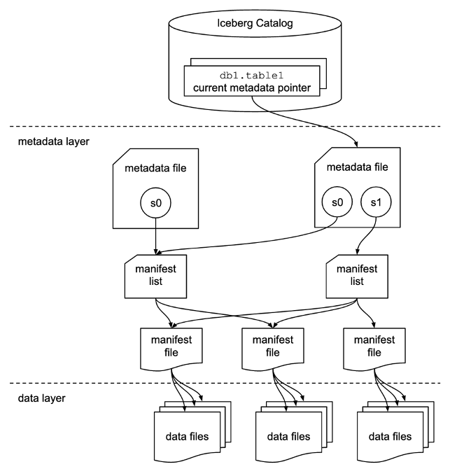
Apache Iceberg addresses customer needs by capturing rich metadata information about the dataset at the time the individual data files are created. There are three layers in the architecture of an Iceberg table: the Iceberg catalog, the metadata layer, and the data layer, as depicted in the following figure (source).

The Iceberg catalog stores the metadata pointer to the current table metadata file. When a select query is reading an Iceberg table, the query engine first goes to the Iceberg catalog, then retrieves the location of the current metadata file. Whenever there is an update to the Iceberg table, a new snapshot of the table is created, and the metadata pointer points to the current table metadata file.

The following is an example Iceberg catalog with AWS Glue implementation. You can see the database name, the location (S3 path) of the Iceberg table, and the metadata location.

The metadata layer has three types of files: the metadata file, manifest list, and manifest file in a hierarchy. At the top of the hierarchy is the metadata file, which stores information about the table’s schema, partition information, and snapshots. The snapshot points to the manifest list. The manifest list has the information about each manifest file that makes up the snapshot, such as location of the manifest file, the partitions it belongs to, and the lower and upper bounds for partition columns for the data files it tracks. The manifest file tracks data files as well as additional details about each file, such as the file format. All three files work in a hierarchy to track the snapshots, schema, partitioning, properties, and data files in an Iceberg table.

The data layer has the individual data files of the Iceberg table. Iceberg supports a wide range of file formats including Parquet, ORC, and Avro. Because the Iceberg table tracks the individual data files instead of only pointing to the partition location with data files, it isolates the writing operations from reading operations. You can write the data files at any time, but only commit the change explicitly, which creates a new version of the snapshot and metadata files.

Solution overview

In this post, we walk you through a solution to build a high-performing Apache Iceberg data lake on Amazon S3; process incremental data with insert, update, and delete SQL statements; and tune the Iceberg table to improve read and write performance. The following diagram illustrates the solution architecture.

To demonstrate this solution, we use the Amazon Customer Reviews dataset in an S3 bucket (s3://amazon-reviews-pds/parquet/). In real use case, it would be raw data stored in your S3 bucket. We can check the data size with the following code in the AWS Command Line Interface (AWS CLI):

//Run this AWS CLI command to check the data size
aws s3 ls --summarize --human-readable --recursive s3://amazon-reviews-pds/parquet

The total object count is 430, and total size is 47.4 GiB.

To set up and test this solution, we complete the following high-level steps:

  1. Set up an S3 bucket in the curated zone to store converted data in Iceberg table format.
  2. Launch an EMR cluster with appropriate configurations for Apache Iceberg.
  3. Create a notebook in EMR Studio.
  4. Configure the Spark session for Apache Iceberg.
  5. Convert data to Iceberg table format and move data to the curated zone.
  6. Run insert, update, and delete queries in Athena to process incremental data.
  7. Carry out performance tuning.

Prerequisites

To follow along with this walkthrough, you must have an AWS account with an AWS Identity and Access Management (IAM) role that has sufficient access to provision the required resources.

Set up the S3 bucket for Iceberg data in the curated zone in your data lake

Choose the Region in which you want to create the S3 bucket and provide a unique name:

s3://iceberg-curated-blog-data

Launch an EMR cluster to run Iceberg jobs using Spark

You can create an EMR cluster from the AWS Management Console, Amazon EMR CLI, or AWS Cloud Development Kit (AWS CDK). For this post, we walk you through how to create an EMR cluster from the console.

  1. On the Amazon EMR console, choose Create cluster.
  2. Choose Advanced options.
  3. For Software Configuration, choose the latest Amazon EMR release. As of January 2023, the latest release is 6.9.0. Iceberg requires release 6.5.0 and above.
  4. Select JupyterEnterpriseGateway and Spark as the software to install.
  5. For Edit software settings, select Enter configuration and enter [{"classification":"iceberg-defaults","properties":{"iceberg.enabled":true}}].
  6. Leave other settings at their default and choose Next.
  7. For Hardware, use the default setting.
  8. Choose Next.
  9. For Cluster name, enter a name. We use iceberg-blog-cluster.
  10. Leave the remaining settings unchanged and choose Next.
  11. Choose Create cluster.

Create a notebook in EMR Studio

We now walk you through how to create a notebook in EMR Studio from the console.

  1. On the IAM console, create an EMR Studio service role.
  2. On the Amazon EMR console, choose EMR Studio.
  3. Choose Get started.

The Get started page appears in a new tab.

  1. Choose Create Studio in the new tab.
  2. Enter a name. We use iceberg-studio.
  3. Choose the same VPC and subnet as those for the EMR cluster, and the default security group.
  4. Choose AWS Identity and Access Management (IAM) for authentication, and choose the EMR Studio service role you just created.
  5. Choose an S3 path for Workspaces backup.
  6. Choose Create Studio.
  7. After the Studio is created, choose the Studio access URL.
  8. On the EMR Studio dashboard, choose Create workspace.
  9. Enter a name for your Workspace. We use iceberg-workspace.
  10. Expand Advanced configuration and choose Attach Workspace to an EMR cluster.
  11. Choose the EMR cluster you created earlier.
  12. Choose Create Workspace.
  13. Choose the Workspace name to open a new tab.

In the navigation pane, there is a notebook that has the same name as the Workspace. In our case, it is iceberg-workspace.

  1. Open the notebook.
  2. When prompted to choose a kernel, choose Spark.

Configure a Spark session for Apache Iceberg

Use the following code, providing your own S3 bucket name:

%%configure -f
{
"conf": {
"spark.sql.catalog.demo": "org.apache.iceberg.spark.SparkCatalog",
"spark.sql.catalog.demo.catalog-impl": "org.apache.iceberg.aws.glue.GlueCatalog",
"spark.sql.catalog.demo.warehouse": "s3://iceberg-curated-blog-data",
"spark.sql.extensions":"org.apache.iceberg.spark.extensions.IcebergSparkSessionExtensions",
"spark.sql.catalog.demo.io-impl":"org.apache.iceberg.aws.s3.S3FileIO"
}
}

This sets the following Spark session configurations:

  • spark.sql.catalog.demo – Registers a Spark catalog named demo, which uses the Iceberg Spark catalog plugin.
  • spark.sql.catalog.demo.catalog-impl – The demo Spark catalog uses AWS Glue as the physical catalog to store Iceberg database and table information.
  • spark.sql.catalog.demo.warehouse – The demo Spark catalog stores all Iceberg metadata and data files under the root path defined by this property: s3://iceberg-curated-blog-data.
  • spark.sql.extensions – Adds support to Iceberg Spark SQL extensions, which allows you to run Iceberg Spark procedures and some Iceberg-only SQL commands (you use this in a later step).
  • spark.sql.catalog.demo.io-impl – Iceberg allows users to write data to Amazon S3 through S3FileIO. The AWS Glue Data Catalog by default uses this FileIO, and other catalogs can load this FileIO using the io-impl catalog property.

Convert data to Iceberg table format

You can use either Spark on Amazon EMR or Athena to load the Iceberg table. In the EMR Studio Workspace notebook Spark session, run the following commands to load the data:

// create a database in AWS Glue named reviews if not exist
spark.sql("CREATE DATABASE IF NOT EXISTS demo.reviews")

// load reviews - this load all the parquet files
val reviews_all_location = "s3://amazon-reviews-pds/parquet/"
val reviews_all = spark.read.parquet(reviews_all_location)

// write reviews data to an Iceberg v2 table
reviews_all.writeTo("demo.reviews.all_reviews").tableProperty("format-version", "2").createOrReplace()

After you run the code, you should find two prefixes created in your data warehouse S3 path (s3://iceberg-curated-blog-data/reviews.db/all_reviews): data and metadata.

Process incremental data using insert, update, and delete SQL statements in Athena

Athena is a serverless query engine that you can use to perform read, write, update, and optimization tasks against Iceberg tables. To demonstrate how the Apache Iceberg data lake format supports incremental data ingestion, we run insert, update, and delete SQL statements on the data lake.

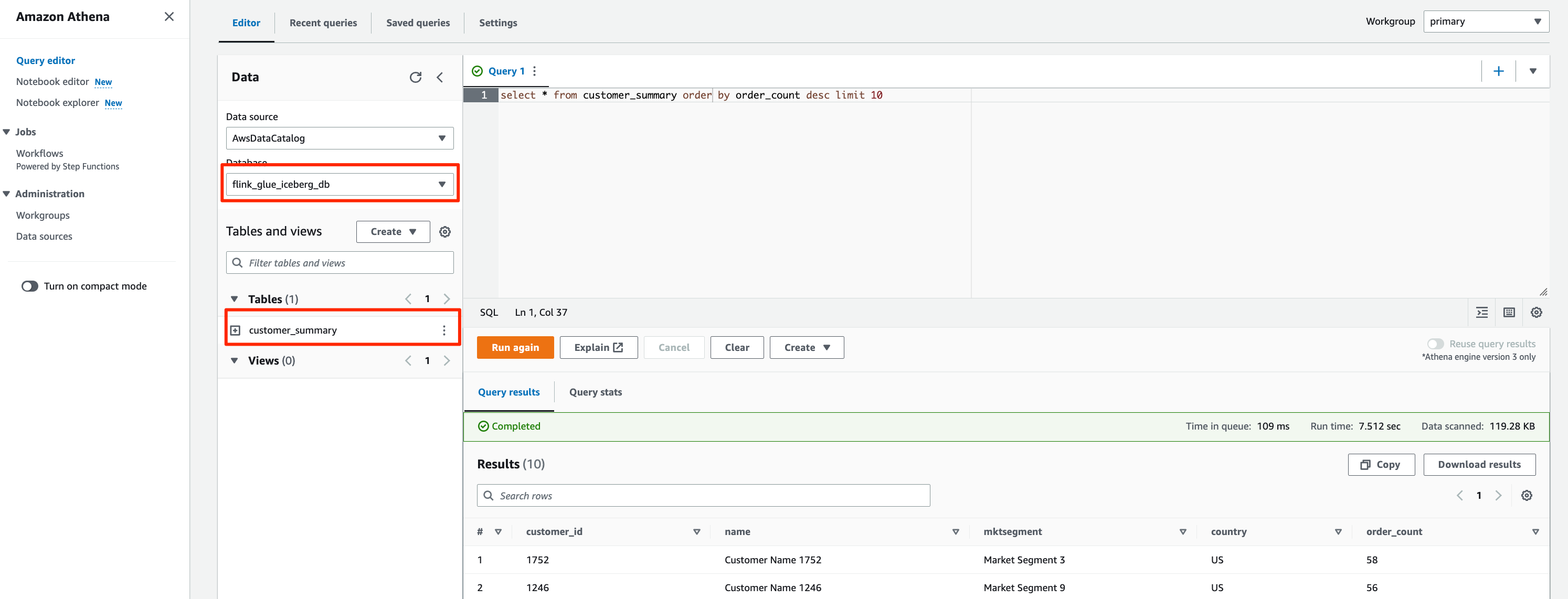
Navigate to the Athena console and choose Query editor. If this is your first time using the Athena query editor, you need to configure the query result location to be the S3 bucket you created earlier. You should be able to see that the table reviews.all_reviews is available for querying. Run the following query to verify that you have loaded the Iceberg table successfully:

select * from reviews.all_reviews limit 5;

Process incremental data by running insert, update, and delete SQL statements:

//Example update statement
update reviews.all_reviews set star_rating=5 where product_category = 'Watches' and star_rating=4

//Example delete statement
delete from reviews.all_reviews where product_category = 'Watches' and star_rating=1

Performance tuning

In this section, we walk through different ways to improve Apache Iceberg read and write performance.

Configure Apache Iceberg table properties

Apache Iceberg is a table format, and it supports table properties to configure table behavior such as read, write, and catalog. You can improve the read and write performance on Iceberg tables by adjusting the table properties.

For example, if you notice that you write too many small files for an Iceberg table, you can config the write file size to write fewer but bigger size files, to help improve query performance.

Property Default Description
write.target-file-size-bytes 536870912 (512 MB) Controls the size of files generated to target about this many bytes

Use the following code to alter the table format:

//Example code to alter table format in EMR Studio Workspace notebook
spark.sql("ALTER TABLE demo.reviews.all_reviews 
SET TBLPROPERTIES ('write_target_data_file_size_bytes'='536870912')")

Partitioning and sorting

To make a query run fast, the less data read the better. Iceberg takes advantage of the rich metadata it captures at write time and facilitates techniques such as scan planning, partitioning, pruning, and column-level stats such as min/max values to skip data files that don’t have match records. We walk you through how query scan planning and partitioning work in Iceberg and how we use them to improve query performance.

Query scan planning

For a given query, the first step in a query engine is scan planning, which is the process to find the files in a table needed for a query. Planning in an Iceberg table is very efficient, because Iceberg’s rich metadata can be used to prune metadata files that aren’t needed, in addition to filtering data files that don’t contain matching data. In our tests, we observed Athena scanned 50% or less data for a given query on an Iceberg table compared to original data before conversion to Iceberg format.

There are two types of filtering:

  • Metadata filtering – Iceberg uses two levels of metadata to track the files in a snapshot: the manifest list and manifest files. It first uses the manifest list, which acts as an index of the manifest files. During planning, Iceberg filters manifests using the partition value range in the manifest list without reading all the manifest files. Then it uses selected manifest files to get data files.
  • Data filtering – After selecting the list of manifest files, Iceberg uses the partition data and column-level stats for each data file stored in manifest files to filter data files. During planning, query predicates are converted to predicates on the partition data and applied first to filter data files. Then, the column stats like column-level value counts, null counts, lower bounds, and upper bounds are used to filter out data files that can’t match the query predicate. By using upper and lower bounds to filter data files at planning time, Iceberg greatly improves query performance.

Partitioning and sorting

Partitioning is a way to group records with the same key column values together in writing. The benefit of partitioning is faster queries that access only part of the data, as explained earlier in query scan planning: data filtering. Iceberg makes partitioning simple by supporting hidden partitioning, in the way that Iceberg produces partition values by taking a column value and optionally transforming it.

In our use case, we first run the following query on the Iceberg table not partitioned. Then we partition the Iceberg table by the category of the reviews, which will be used in the query WHERE condition to filter out records. With partitioning, the query could scan much less data. See the following code:

//Example code in EMR Studio Workspace notebook to create an Iceberg table all_reviews_partitioned partitioned by product_category
reviews_all.writeTo("demo.reviews.all_reviews_partitioned").tableProperty("format-version", "2").partitionedBy($"product_category").createOrReplace()

Run the following select statement on the non-partitioned all_reviews table vs. the partitioned table to see the performance difference:

//Run this query on all_reviews table and the partitioned table for performance testing
select marketplace,customer_id, review_id,product_id,product_title,star_rating from reviews.all_reviews where product_category = 'Watches' and review_date between date('2005-01-01') and date('2005-03-31')

//Run the same select query on partitioned dataset
select marketplace,customer_id, review_id,product_id,product_title,star_rating from reviews.all_reviews_partitioned where product_category = 'Watches' and review_date between date('2005-01-01') and date('2005-03-31')

The following table shows the performance improvement of data partitioning, with about 50% performance improvement and 70% less data scanned.

Dataset Name Non-Partitioned Dataset Partitioned Dataset
Runtime (seconds) 8.20 4.25
Data Scanned (MB) 131.55 33.79

Note that the runtime is the average runtime with multiple runs in our test.

We saw good performance improvement after partitioning. However, this can be further improved by using column-level stats from Iceberg manifest files. In order to use the column-level stats effectively, you want to further sort your records based on the query patterns. Sorting the whole dataset using the columns that are often used in queries will reorder the data in such a way that each data file ends up with a unique range of values for the specific columns. If these columns are used in the query condition, it allows query engines to further skip data files, thereby enabling even faster queries.

Copy-on-write vs. read-on-merge

When implementing update and delete on Iceberg tables in the data lake, there are two approaches defined by the Iceberg table properties:

  • Copy-on-write – With this approach, when there are changes to the Iceberg table, either updates or deletes, the data files associated with the impacted records will be duplicated and updated. The records will be either updated or deleted from the duplicated data files. A new snapshot of the Iceberg table will be created and pointing to the newer version of data files. This makes the overall writes slower. There might be situations that concurrent writes are needed with conflicts so retry has to happen, which increases the write time even more. On the other hand, when reading the data, there is no extra process needed. The query will retrieve data from the latest version of data files.
  • Merge-on-read – With this approach, when there are updates or deletes on the Iceberg table, the existing data files will not be rewritten; instead new delete files will be created to track the changes. For deletes, a new delete file will be created with the deleted records. When reading the Iceberg table, the delete file will be applied to the retrieved data to filter out the delete records. For updates, a new delete file will be created to mark the updated records as deleted. Then a new file will be created for those records but with updated values. When reading the Iceberg table, both the delete and new files will be applied to the retrieved data to reflect the latest changes and produce the correct results. So, for any subsequent queries, an extra step to merge the data files with the delete and new files will happen, which will usually increase the query time. On the other hand, the writes might be faster because there is no need to rewrite the existing data files.

To test the impact of the two approaches, you can run the following code to set the Iceberg table properties:

//Run code to alter Iceberg table property to set copy-on-write and merge-on-read in EMR Studio Workspace notebook
spark.sql(“ALTER TABLE demo.reviews.all_reviews 
SET TBLPROPERTIES (‘write.delete.mode’=’copy-on-write’,’write.update.mode’=’copy-on-write’)”)

Run the update, delete, and select SQL statements in Athena to show the runtime difference for copy-on-write vs. merge-on-read:

//Example update statement
update reviews.all_reviews set star_rating=5 where product_category = ‘Watches’ and star_rating=4

//Example delete statement
delete from reviews.all_reviews where product_category = ‘Watches’ and star_rating=1

//Example select statement
select marketplace,customer_id, review_id,product_id,product_title,star_rating from reviews.all_reviews where product_category = ‘Watches’ and review_date between date(‘2005-01-01’) and date(‘2005-03-31’)

The following table summarizes the query runtimes.

Query Copy-on-Write Merge-on-Read
UPDATE DELETE SELECT UPDATE DELETE SELECT
Runtime (seconds) 66.251 116.174 97.75 10.788 54.941 113.44
Data scanned (MB) 494.06 3.07 137.16 494.06 3.07 137.16

Note that the runtime is the average runtime with multiple runs in our test.

As our test results show, there are always trade-offs in the two approaches. Which approach to use depends on your use cases. In summary, the considerations come down to latency on the read vs. write. You can reference the following table and make the right choice.

. Copy-on-Write Merge-on-Read
Pros Faster reads Faster writes
Cons Expensive writes Higher latency on reads
When to use Good for frequent reads, infrequent updates and deletes or large batch updates Good for tables with frequent updates and deletes

Data compaction

If your data file size is small, you might end up with thousands or millions of files in an Iceberg table. This dramatically increases the I/O operation and slows down the queries. Furthermore, Iceberg tracks each data file in a dataset. More data files lead to more metadata. This in turn increases the overhead and I/O operation on reading metadata files. In order to improve the query performance, it’s recommended to compact small data files to larger data files.

When updating and deleting records in Iceberg table, if the read-on-merge approach is used, you might end up with many small deletes or new data files. Running compaction will combine all these files and create a newer version of the data file. This eliminates the need to reconcile them during reads. It’s recommended to have regular compaction jobs to impact reads as little as possible while still maintaining faster write speed.

Run the following data compaction command, then run the select query from Athena:

//Data compaction 
optimize reviews.all_reviews REWRITE DATA USING BIN_PACK

//Run this query before and after data compaction
select marketplace,customer_id, review_id,product_id,product_title,star_rating from reviews.all_reviews where product_category = 'Watches' and review_date between date('2005-01-01') and date('2005-03-31')

The following table compares the runtime before vs. after data compaction. You can see about 40% performance improvement.

Query Before Data Compaction After Data Compaction
Runtime (seconds) 97.75 32.676 seconds
Data scanned (MB) 137.16 M 189.19 M

Note that the select queries ran on the all_reviews table after update and delete operations, before and after data compaction. The runtime is the average runtime with multiple runs in our test.

Clean up

After you follow the solution walkthrough to perform the use cases, complete the following steps to clean up your resources and avoid further costs:

  1. Drop the AWS Glue tables and database from Athena or run the following code in your notebook:
// DROP the table 
spark.sql("DROP TABLE demo.reviews.all_reviews") 
spark.sql("DROP TABLE demo.reviews.all_reviews_partitioned") 

// DROP the database 
spark.sql("DROP DATABASE demo.reviews")
  1. On the EMR Studio console, choose Workspaces in the navigation pane.
  2. Select the Workspace you created and choose Delete.
  3. On the EMR console, navigate to the Studios page.
  4. Select the Studio you created and choose Delete.
  5. On the EMR console, choose Clusters in the navigation pane.
  6. Select the cluster and choose Terminate.
  7. Delete the S3 bucket and any other resources that you created as part of the prerequisites for this post.

Conclusion

In this post, we introduced the Apache Iceberg framework and how it helps resolve some of the challenges we have in a modern data lake. Then we walked you though a solution to process incremental data in a data lake using Apache Iceberg. Finally, we had a deep dive into performance tuning to improve read and write performance for our use cases.

We hope this post provides some useful information for you to decide whether you want to adopt Apache Iceberg in your data lake solution.


About the Authors

Flora Wu is a Sr. Resident Architect at AWS Data Lab. She helps enterprise customers create data analytics strategies and build solutions to accelerate their businesses outcomes. In her spare time, she enjoys playing tennis, dancing salsa, and traveling.

Daniel Li is a Sr. Solutions Architect at Amazon Web Services. He focuses on helping customers develop, adopt, and implement cloud services and strategy. When not working, he likes spending time outdoors with his family.

Build a semantic search engine for tabular columns with Transformers and Amazon OpenSearch Service

Post Syndicated from Kachi Odoemene original https://aws.amazon.com/blogs/big-data/build-a-semantic-search-engine-for-tabular-columns-with-transformers-and-amazon-opensearch-service/

Finding similar columns in a data lake has important applications in data cleaning and annotation, schema matching, data discovery, and analytics across multiple data sources. The inability to accurately find and analyze data from disparate sources represents a potential efficiency killer for everyone from data scientists, medical researchers, academics, to financial and government analysts.

Conventional solutions involve lexical keyword search or regular expression matching, which are susceptible to data quality issues such as absent column names or different column naming conventions across diverse datasets (for example, zip_code, zcode, postalcode).

In this post, we demonstrate a solution for searching for similar columns based on column name, column content, or both. The solution uses approximate nearest neighbors algorithms available in Amazon OpenSearch Service to search for semantically similar columns. To facilitate the search, we create features representations (embeddings) for individual columns in the data lake using pre-trained Transformer models from the sentence-transformers library in Amazon SageMaker. Finally, to interact with and visualize results from our solution, we build an interactive Streamlit web application running on AWS Fargate.

We include a code tutorial for you to deploy the resources to run the solution on sample data or your own data.

Solution overview

The following architecture diagram illustrates the two-stage workflow for finding semantically similar columns. The first stage runs an AWS Step Functions workflow that creates embeddings from tabular columns and builds the OpenSearch Service search index. The second stage, or the online inference stage, runs a Streamlit application through Fargate. The web application collects input search queries and retrieves from the OpenSearch Service index the approximate k-most-similar columns to the query.

Solution architecture

Figure 1. Solution architecture

The automated workflow proceeds in the following steps:

  1. The user uploads tabular datasets into an Amazon Simple Storage Service (Amazon S3) bucket, which invokes an AWS Lambda function that initiates the Step Functions workflow.
  2. The workflow begins with an AWS Glue job that converts the CSV files into Apache Parquet data format.
  3. A SageMaker Processing job creates embeddings for each column using pre-trained models or custom column embedding models. The SageMaker Processing job saves the column embeddings for each table in Amazon S3.
  4. A Lambda function creates the OpenSearch Service domain and cluster to index the column embeddings produced in the previous step.
  5. Finally, an interactive Streamlit web application is deployed with Fargate. The web application provides an interface for the user to input queries to search the OpenSearch Service domain for similar columns.

You can download the code tutorial from GitHub to try this solution on sample data or your own data. Instructions on the how to deploy the required resources for this tutorial are available on Github.

Prerequistes

To implement this solution, you need the following:

  • An AWS account.
  • Basic familiarity with AWS services such as the AWS Cloud Development Kit (AWS CDK), Lambda, OpenSearch Service, and SageMaker Processing.
  • A tabular dataset to create the search index. You can bring your own tabular data or download the sample datasets on GitHub.

Build a search index

The first stage builds the column search engine index. The following figure illustrates the Step Functions workflow that runs this stage.

Step functions workflow

Figure 2 – Step functions workflow – multiple embedding models

Datasets

In this post, we build a search index to include over 400 columns from over 25 tabular datasets. The datasets originate from the following public sources:

For the the full list of the tables included in the index, see the code tutorial on GitHub.

You can bring your own tabular dataset to augment the sample data or build your own search index. We include two Lambda functions that initiate the Step Functions workflow to build the search index for individual CSV files or a batch of CSV files, respectively.

Transform CSV to Parquet

Raw CSV files are converted to Parquet data format with AWS Glue. Parquet is a column-oriented format file format preferred in big data analytics that provides efficient compression and encoding. In our experiments, the Parquet data format offered significant reduction in storage size compared to raw CSV files. We also used Parquet as a common data format to convert other data formats (for example JSON and NDJSON) because it supports advanced nested data structures.

Create tabular column embeddings

To extract embeddings for individual table columns in the sample tabular datasets in this post, we use the following pre-trained models from the sentence-transformers library. For additional models, see Pretrained Models.

Model name Dimension Size (MB)
all-MiniLM-L6-v2 384 80
all-distilroberta-v1 768 290
average_word_embeddings_glove.6B.300d 300 420

The SageMaker Processing job runs create_embeddings.py(code) for a single model. For extracting embeddings from multiple models, the workflow runs parallel SageMaker Processing jobs as shown in the Step Functions workflow. We use the model to create two sets of embeddings:

  • column_name_embeddings – Embeddings of column names (headers)
  • column_content_embeddings – Average embedding of all the rows in the column

For more information about the column embedding process, see the code tutorial on GitHub.

An alternative to the SageMaker Processing step is to create a SageMaker batch transform to get column embeddings on large datasets. This would require deploying the model to a SageMaker endpoint. For more information, see Use Batch Transform.

Index embeddings with OpenSearch Service

In the final step of this stage, a Lambda function adds the column embeddings to a OpenSearch Service approximate k-Nearest-Neighbor (kNN) search index. Each model is assigned its own search index. For more information about the approximate kNN search index parameters, see k-NN.

Online inference and semantic search with a web app

The second stage of the workflow runs a Streamlit web application where you can provide inputs and search for semantically similar columns indexed in OpenSearch Service. The application layer uses an Application Load Balancer, Fargate, and Lambda. The application infrastructure is automatically deployed as part of the solution.

The application allows you to provide an input and search for semantically similar column names, column content, or both. Additionally, you can select the embedding model and number of nearest neighbors to return from the search. The application receives inputs, embeds the input with the specified model, and uses kNN search in OpenSearch Service to search indexed column embeddings and find the most similar columns to the given input. The search results displayed include the table names, column names, and similarity scores for the columns identified, as well as the locations of the data in Amazon S3 for further exploration.

The following figure shows an example of the web application. In this example, we searched for columns in our data lake that have similar Column Names (payload type) to district (payload). The application used all-MiniLM-L6-v2 as the embedding model and returned 10 (k) nearest neighbors from our OpenSearch Service index.

The application returned transit_district, city, borough, and location as the four most similar columns based on the data indexed in OpenSearch Service. This example demonstrates the ability of the search approach to identify semantically similar columns across datasets.

Web application user interface

Figure 3: Web application user interface

Clean up

To delete the resources created by the AWS CDK in this tutorial, run the following command:

cdk destroy --all

Conclusion

In this post, we presented an end-to-end workflow for building a semantic search engine for tabular columns.

Get started today on your own data with our code tutorial available on GitHub. If you’d like help accelerating your use of ML in your products and processes, please contact the Amazon Machine Learning Solutions Lab.


About the Authors

Kachi Odoemene is an Applied Scientist at AWS AI. He builds AI/ML solutions to solve business problems for AWS customers.

Taylor McNally is a Deep Learning Architect at Amazon Machine Learning Solutions Lab. He helps customers from various industries build solutions leveraging AI/ML on AWS. He enjoys a good cup of coffee, the outdoors, and time with his family and energetic dog.

Austin Welch is a Data Scientist in the Amazon ML Solutions Lab. He develops custom deep learning models to help AWS public sector customers accelerate their AI and cloud adoption. In his spare time, he enjoys reading, traveling, and jiu-jitsu.
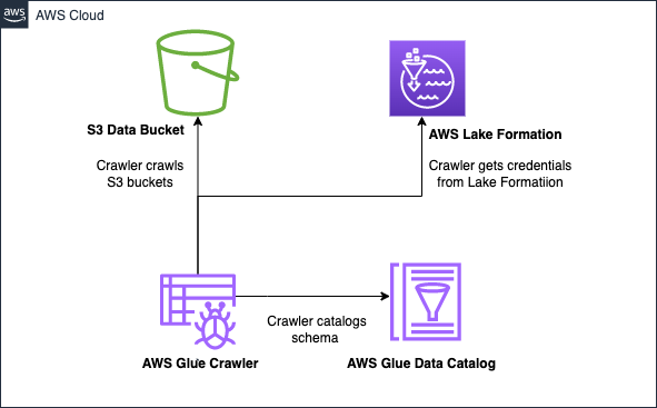
AWS Week in Review – February 27, 2023

Post Syndicated from Antje Barth original https://aws.amazon.com/blogs/aws/aws-week-in-review-february-27-2023/

A couple days ago, I had the honor of doing a live stream on generative AI, discussing recent innovations and concepts behind the current generation of large language and vision models and how we got there. In today’s roundup of news and announcements, I will share some additional information—including an expanded partnership to make generative AI more accessible, a blog post about diffusion models, and our weekly Twitch show on Generative AI. Let’s dive right into it!

Last Week’s Launches
Here are some launches that got my attention during the previous week:

Integrated Private Wireless on AWS – The Integrated Private Wireless on AWS program is designed to provide enterprises with managed and validated private wireless offerings from leading communications service providers (CSPs). The offerings integrate CSPs’ private 5G and 4G LTE wireless networks with AWS services across AWS Regions, AWS Local Zones, AWS Outposts, and AWS Snow Family. For more details, read this Industries Blog post and check out this eBook. And, if you’re attending the Mobile World Congress Barcelona this week, stop by the AWS booth at the Upper Walkway, South Entrance, at the Fira Barcelona Gran Via, to learn more.

AWS Glue Crawlers – Now integrate with Lake Formation. AWS Glue Crawlers are used to discover datasets, extract schema information, and populate the AWS Glue Data Catalog. With this Glue Crawler and Lake Formation integration, you can configure a crawler to use Lake Formation permissions to access an S3 data store or a Data Catalog table with an underlying S3 location within the same AWS account or another AWS account. You can configure an existing Data Catalog table as a crawler’s target if the crawler and the Data Catalog table reside in the same account. To learn more, check out this Big Data Blog post.

AWS Glue Crawlers now support integration with AWS Lake Formation

Amazon SageMaker Model Monitor – You can now launch and configure Amazon SageMaker Model Monitor from the SageMaker Model Dashboard using a code-free point-and-click setup experience. SageMaker Model Dashboard gives you unified monitoring across all your models by providing insights into deviations from expected behavior, automated alerts, and troubleshooting to improve model performance. Model Monitor can detect drift in data quality, model quality, bias, and feature attribution and alert you to take remedial actions when such changes occur.

Amazon EKS – Now supports Kubernetes version 1.25. Kubernetes 1.25 introduced several new features and bug fixes, and you can now use Amazon EKS and Amazon EKS Distro to run Kubernetes version 1.25. You can create new 1.25 clusters or upgrade your existing clusters to 1.25 using the Amazon EKS console, the eksctl command line interface, or through an infrastructure-as-code tool. To learn more about this release named “Combiner,” check out this Containers Blog post.

Amazon Detective – New self-paced workshop available. You can now learn to use Amazon Detective with a new self-paced workshop in AWS Workshop Studio. AWS Workshop Studio is a collection of self-paced tutorials designed to teach practical skills and techniques to solve business problems. The Amazon Detective workshop is designed to teach you how to use the primary features of Detective through a series of interactive modules that cover topics such as security alert triage, security incident investigation, and threat hunting. Get started with the Amazon Detective Workshop.

For a full list of AWS announcements, be sure to keep an eye on the What’s New at AWS page.

Other AWS News
Here are some additional news items and blog posts that you may find interesting:

🤗❤☁ AWS and Hugging Face collaborate to make generative AI more accessible and cost-efficient – This previous week, we announced an expanded collaboration between AWS and Hugging Face to accelerate the training, fine-tuning, and deployment of large language and vision models used to create generative AI applications. Generative AI applications can perform a variety of tasks, including text summarization, answering questions, code generation, image creation, and writing essays and articles. For more details, read this Machine Learning Blog post.

If you are interested in generative AI, I also recommend reading this blog post on how to Fine-tune text-to-image Stable Diffusion models with Amazon SageMaker JumpStart. Stable Diffusion is a deep learning model that allows you to generate realistic, high-quality images and stunning art in just a few seconds. This blog post discusses how to make design choices, including dataset quality, size of training dataset, choice of hyperparameter values, and applicability to multiple datasets.

AWS open-source news and updates – My colleague Ricardo writes this weekly open-source newsletter in which he highlights new open-source projects, tools, and demos from the AWS Community. Read edition #146 here.

Upcoming AWS Events
Check your calendars and sign up for these AWS events:

Build On AWS - Generative AI#BuildOn Generative AI – Join our weekly live Build On Generative AI Twitch show. Every Monday morning, 9:00 US PT, my colleagues Emily and Darko take a look at aspects of generative AI. They host developers, scientists, startup founders, and AI leaders and discuss how to build generative AI applications on AWS.

In today’s episode, my colleague Chris walked us through an end-to-end ML pipeline from data ingestion to fine-tuning and deployment of generative AI models. You can watch the video here.

AWS Pi Day 2023 SmallAWS Pi Day – Join me on March 14 for the third annual AWS Pi Day live, virtual event hosted on the AWS On Air channel on Twitch as we celebrate the 17th birthday of Amazon S3 and the cloud.
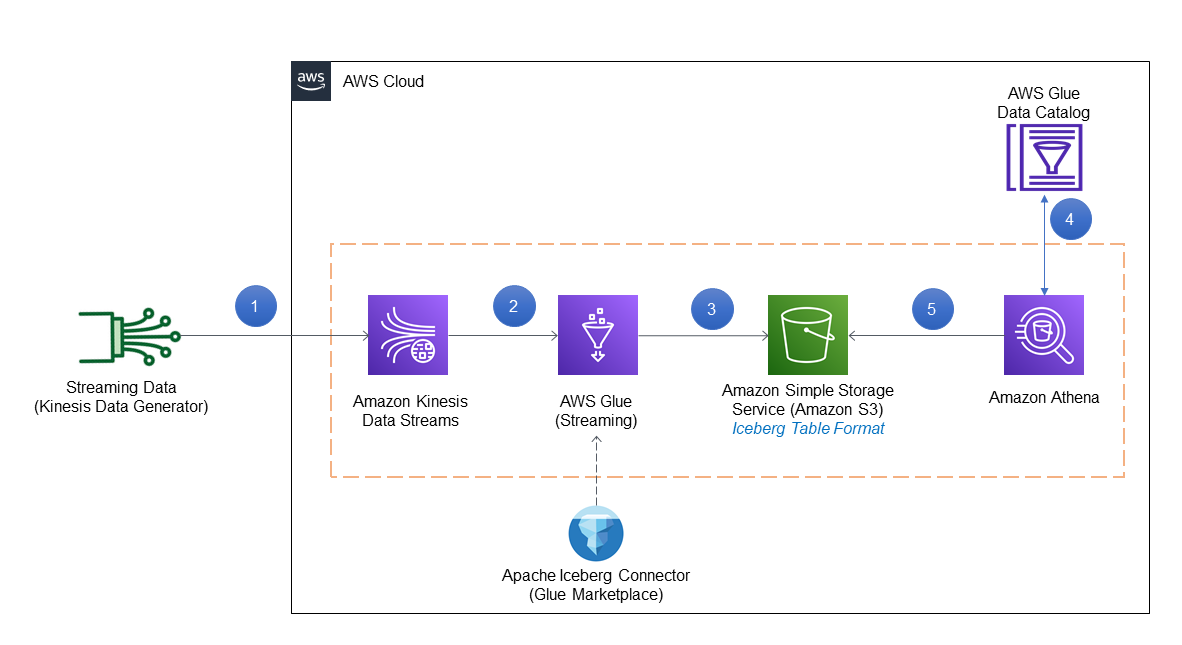
We will discuss the latest innovations across AWS Data services, from storage to analytics and AI/ML. If you are curious about how AI can transform your business, register here and join my session.

AWS Innovate Data and AI/ML edition – AWS Innovate is a free online event to learn the latest from AWS experts and get step-by-step guidance on using AI/ML to drive fast, efficient, and measurable results. Register now for EMEA (March 9) and the Americas (March 14).

You can browse all upcoming AWS-led in-person, virtual events and developer focused events such as Community Days.

That’s all for this week. Check back next Monday for another Week in Review!

— Antje

This post is part of our Week in Review series. Check back each week for a quick roundup of interesting news and announcements from AWS!

Build a real-time GDPR-aligned Apache Iceberg data lake

Post Syndicated from Dhiraj Thakur original https://aws.amazon.com/blogs/big-data/build-a-real-time-gdpr-aligned-apache-iceberg-data-lake/

Data lakes are a popular choice for today’s organizations to store their data around their business activities. As a best practice of a data lake design, data should be immutable once stored. But regulations such as the General Data Protection Regulation (GDPR) have created obligations for data operators who must be able to erase or update personal data from their data lake when requested.

A data lake built on AWS uses Amazon Simple Storage Service (Amazon S3) as its primary storage environment. When a customer asks to erase or update private data, the data lake operator needs to find the required objects in Amazon S3 that contain the required data and take steps to erase or update that data. This activity can be a complex process for the following reasons:

  • Data lakes may contain many S3 objects (each may contain multiple rows), and often it’s difficult to find the object containing the exact data that needs to be erased or personally identifiable information (PII) to be updated as per the request
  • By nature, S3 objects are immutable and therefore applying direct row-based transactions like DELETE or UPDATE isn’t possible

To handle these situations, a transactional feature on S3 objects is required, and frameworks such as Apache Hudi or Apache Iceberg provide you the transactional feature for upserts in Amazon S3.

AWS contributed the Apache Iceberg integration with the AWS Glue Data Catalog, which enables you to use open-source data computation engines like Apache Spark with Iceberg on AWS Glue. In 2022, Amazon Athena announced support of Iceberg, enabling transaction queries on S3 objects.

In this post, we show you how to stream real-time data to an Iceberg table in Amazon S3 using AWS Glue streaming and perform transactions using Amazon Athena for deletes and updates. We use a serverless mechanism for this implementation, which requires minimum operational overhead to manage and fine-tune various configuration parameters, and enables you to extend your use case to ACID operations beyond the GDPR.

Solution overview

We used the Amazon Kinesis Data Generator (KDG) to produce synthetic streaming data in Amazon Kinesis Data Streams and then processed the streaming input data using AWS Glue streaming to store the data in Amazon S3 in Iceberg table format. As part of the customer’s request, we ran delete and update statements using Athena with Iceberg support.

The following diagram illustrates the solution architecture.

The solution workflow consists of the following steps:

  1. Streaming data is generated in JSON format using the KDG template and inserted into Kinesis Data Streams.
  2. An AWS Glue streaming job is connected to Kinesis Data Streams to process the data using the Iceberg connector.
  3. The streaming job output is stored in Amazon S3 in Iceberg table format.
  4. Athena uses the AWS Glue Data Catalog to store and retrieve table metadata for the Amazon S3 data in Iceberg format.
  5. Athena interacts with the Data Catalog tables in Iceberg format for transactional queries required for GDPR.

The codebase required for this post is available in the GitHub repository.

Prerequisites

Before starting the implementation, make sure the following prerequisites are met:

Deploy resources using AWS CloudFormation

Complete the following steps to deploy your solution resources:

  1. After you sign in to your AWS account, launch the CloudFormation template by choosing Launch Stack:
  2. For Stack name, enter a name.
  3. For Username, enter the user name for the KDG.
  4. For Password, enter the password for the KDG (this must be at least six alphanumeric characters, and contain at least one number).
  5. For IAMGlueStreamingJobRoleName, enter a name for the IAM role used for the AWS Glue streaming job.
  6. Choose Next and create your stack.

This CloudFormation template configures the following resources in your account:

  • An S3 bucket named streamingicebergdemo-XX (note that the XX part is a random unique number to make the S3 bucket name unique)
  • An IAM policy and role
  • The KDG URL used for creating synthetic data
  1. After you complete the setup, go to the Outputs tab of the CloudFormation stack to get the S3 bucket name, AWS Glue job execution role (as per your input), and KDG URL.
  2. Before proceeding with the demo, create a folder named custdata under the created S3 bucket.

Create a Kinesis data stream

We use Kinesis Data Streams to create a serverless streaming data service that is built to handle millions of events with low latency. The following steps guide you on how to create the data stream in the us-east-1 Region:

  1. Log in to the AWS Management Console.
  2. Navigate to Kinesis console (make sure the Region is us-east-1).
  3. Select Kinesis Data Streams and choose Create data stream.
  4. For Data stream name, enter demo-data-stream.
  5. For this post, we select On-demand as the Kinesis data stream capacity mode.

On-demand mode works to eliminate the need for provisioning and managing the capacity for streaming data. However, you can implement this solution with Kinesis Data Streams in provisioned mode as well.

  1. Choose Create data stream.
  2. Wait for successful creation of demo-data-stream and for it to be in Active status.

Set up the Kinesis Data Generator

To create a sample streaming dataset, we use the KDG URL generated on the CloudFormation stack Outputs tab and log in with the credentials used in the parameters for the CloudFormation template. For this post, we use the following template to generate sample data in the demo-data-stream Kinesis data stream.

  1. Log in to the KDG URL with the user name and password you supplied during stack creation.
  2. Change the Region to us-east-1.
  3. Select the Kinesis data stream demo-data-stream.
  4. For Records per second, choose Constant and enter 100 (it can be another number, depending on the rate of record creation).
  5. On the Template 1 tab, enter the KDG data generation template:
{
"year": "{{random.number({"min":2000,"max":2022})}}",
"month": "{{random.number({"min":1,"max":12})}}",
"day": "{{random.number({"min":1,"max":30})}}",
"hour": "{{random.number({"min":0,"max":24})}}",
"minute": "{{random.number({"min":0,"max":60})}}",
"customerid": {{random.number({"min":5023,"max":59874})}},
"firstname" : "{{name.firstName}}",
"lastname" : "{{name.lastName}}",
"dateofbirth" : "{{date.past(70)}}",
"city" : "{{address.city}}",
"buildingnumber" : {{random.number({"min":63,"max":947})}},
"streetaddress" : "{{address.streetAddress}}",
"state" : "{{address.state}}",
"zipcode" : "{{address.zipCode}}",
"country" : "{{address.country}}",
"countrycode" : "{{address.countryCode}}",
"phonenumber" : "{{phone.phoneNumber}}",
"productname" : "{{commerce.productName}}",
"transactionamount": {{random.number(
{
"min":10,
"max":150
}
)}}
}
  1. Choose Test template to test the sample records.
  2. When the testing is correct, choose Send data.

This will start sending 100 records per second in the Kinesis data stream. (To stop sending data, choose Stop Sending Data to Kinesis.)

Integrate Iceberg with AWS Glue

To add the Apache Iceberg Connector for AWS Glue, complete the following steps. The connector is free to use and supports AWS Glue 1.0, 2.0, and 3.0.

  1. On the AWS Glue console, choose AWS Glue Studio in the navigation pane.
  2. In the navigation pane, navigate to AWS Marketplace.
  3. Search for and choose Apache Iceberg Connector for AWS Glue.
  4. Choose Accept Terms and Continue to Subscribe.
  5. Choose Continue to Configuration.
  6. For Fulfillment option, choose your AWS Glue version.
  7. For Software version, choose the latest software version.
  8. Choose Continue to Launch.
  9. Under Usage Instructions, choose the link to activate the connector.
  10. Enter a name for the connection, then choose Create connection and activate the connector.
  11. Verify the new connector on the AWS Glue Studio Connectors.

Create the AWS Glue Data Catalog database

The AWS Glue Data Catalog contains references to data that is used as sources and targets of your extract, transform, and load (ETL) jobs in AWS Glue. To create your data warehouse or data lake, you must catalog this data. The AWS Glue Data Catalog is an index to the location and schema of your data. You use the information in the Data Catalog to create and monitor your ETL jobs.

For this post, we create a Data Catalog database named icebergdemodb containing the metadata information of a table named customer, which will be queried through Athena.

  1. On the AWS Glue console, choose Databases in the navigation pane.
  2. Choose Add database.
  3. For Database name, enter icebergdemodb.

This creates an AWS Glue database for metadata storage.

Create a Data Catalog table in Iceberg format

In this step, we create a Data Catalog table in Iceberg table format.

  1. On the Athena console, create an Athena workgroup named demoworkgroup for SQL queries.
  2. Choose Athena engine version 3 for Query engine version.

For more information about Athena versions, refer to Changing Athena engine versions.

  1. Enter the S3 bucket location for Query result configuration under Additional configurations.
  2. Open the Athena query editor and choose demoworkgroup.
  3. Choose the database icebergdemodb.
  4. Enter and run the following DDL to create a table pointing to the Data Catalog database icerbergdemodb. Note that the TBLPROPERTIES section mentions ICEBERG as the table type and LOCATION points to the S3 folder (custdata) URI created in earlier steps. This DDL command is available on the GitHub repo.
CREATE TABLE icebergdemodb.customer(
year string,
month string,
day string,
hour string,
minute string,
customerid string,
firstname string,
lastname string,
dateofbirth string,
city string,
buildingnumber string,
streetaddress string,
state string,
zipcode string,
country string,
countrycode string,
phonenumber string,
productname string,
transactionamount int)
LOCATION '<S3 Location URI>'
TBLPROPERTIES (
'table_type'='ICEBERG',
'format'='parquet',
'write_target_data_file_size_bytes'='536870912',
'optimize_rewrite_delete_file_threshold'='10'
);

After you run the command successfully, you can see the table customer in the Data Catalog.

Create an AWS Glue streaming job

In this section, we create the AWS Glue streaming job, which fetches the record from the Kinesis data stream using the Spark script editor.

  1. On the AWS Glue console, choose Jobs (new) in the navigation pane.
  2. For Create job¸ select Spark script editor.
  3. For Options¸ select Create a new script with boilerplate code.
  4. Choose Create.
  5. Enter the code available in the GitHub repo in the editor.

The sample code keeps appending data in the target location by fetching records from the Kinesis data stream.

  1. Choose the Job details tab in the query editor.
  2. For Name, enter Demo_Job.
  3. For IAM role¸ choose demojobrole.
  4. For Type, choose Spark Streaming.
  5. For Glue Version, choose Glue 3.0.
  6. For Language, choose Python 3.
  7. For Worker type, choose G 0.25X.
  8. Select Automatically scale the number of workers.
  9. For Maximum number of workers, enter 5.
  10. Under Advanced properties, select Use Glue Data Catalog as the Hive metastore.
  11. For Connections, choose the connector you created.
  12. For Job parameters, enter the following key pairs (provide your S3 bucket and account ID):
Key Value
--iceberg_job_catalog_warehouse s3://streamingicebergdemo-XX/custdata/
--output_path s3://streamingicebergdemo-XX
--kinesis_arn arn:aws:kinesis:us-east-1:<AWS Account ID>:stream/demo-data-stream
--user-jars-first True

  1. Choose Run to start the AWS Glue streaming job.
  2. To monitor the job, choose Monitoring in the navigation pane.
  3. Select Demo_Job and choose View run details to check the job run details and Amazon CloudWatch logs.

Run GDPR use cases on Athena

In this section, we demonstrate a few use cases that are relevant to GDPR alignment with the user data that’s stored in Iceberg format in the Amazon S3-based data lake as implemented in the previous steps. For this, let’s consider that the following requests are being initiated in the workflow to comply with the regulations:

  • Delete the records for the input customerid (for example, 59289)
  • Update phonenumber for the customerid (for example, 51842)

The IDs used in this example are samples only because they were created through the KDG template used earlier, which creates sample data. You can search for IDs in your implementation by querying through the Athena query editor. The steps remain the same.

Delete data by customer ID

Complete the following steps to fulfill the first use case:

  1. On the Athena console, and make sure icebergdemodb is chosen as the database.
  2. Open the query editor.
  3. Enter the following query using a customer ID and choose Run:
SELECT count(*)
FROM icebergdemodb.customer
WHERE customerid = '59289';

This query gives the count of records for the input customerid before delete.

  1. Enter the following query with the same customer ID and choose Run:
MERGE INTO icebergdemodb.customer trg
USING (SELECT customerid
FROM icebergdemodb.customer
WHERE customerid = '59289') src
ON (trg.customerid = src.customerid)
WHEN MATCHED
THEN DELETE;

This query deletes the data for the input customerid as per the workflow generated.

  1. Test if there is data with the customer ID using a count query.

The count should be 0.

Update data by customer ID

Complete the following steps to test the second use case:

  1. On the Athena console, make sure icebergdemodb is chosen as the database.
  2. Open the query editor.
  3. Enter the following query with a customer ID and choose Run.
SELECT customerid, phonenumber
FROM icebergdemodb.customer
WHERE customerid = '51936';

This query gives the value for phonenumber before update.

  1. Run the following query to update the required columns:
MERGE INTO icebergdemodb.customer trg
USING (SELECT customerid
FROM icebergdemodb.customer
WHERE customerid = '51936') src
ON (trg.customerid = src.customerid)
WHEN MATCHED
THEN UPDATE SET phonenumber = '000';

This query updates the data to a dummy value.

  1. Run the SELECT query to check the update.

You can see the data is updated correctly.

Vacuum table

A good practice is to run the VACUUM command periodically on the table because operations like INSERT, UPDATE, DELETE, and MERGE will take place on the Iceberg table. See the following code:

VACUUM icebergdemodb.customer;

Considerations

The following are a few considerations to keep in mind for this implementation:

Clean up

Complete the following steps to clean up the resources you created for this post:

    1. Delete the custdata folder in the S3 bucket.
    2. Delete the CloudFormation stack.
    3. Delete the Kinesis data stream.
    4. Delete the S3 bucket storing the data.
    5. Delete the AWS Glue job and Iceberg connector.
    6. Delete the AWS Glue Data Catalog database and table.
    7. Delete the Athena workgroup.
    8. Delete the IAM roles and policies.

Conclusion

This post explained how you can use the Iceberg table format on Athena to implement GDPR use cases like data deletion and data upserts as required, when streaming data is being generated and ingested through AWS Glue streaming jobs in Amazon S3.

The operations for the Iceberg table that we demonstrated in this post aren’t all of the data operations that Iceberg supports. Refer to the Apache Iceberg documentation for details on various operations.


About the Authors

Dhiraj Thakur is a Solutions Architect with Amazon Web Services. He works with AWS customers and partners to provide guidance on enterprise cloud adoption, migration, and strategy. He is passionate about technology and enjoys building and experimenting in the analytics and AI/ML space.

Rajdip Chaudhuri is Solutions Architect with Amazon Web Services specializing in data and analytics. He enjoys working with AWS customers and partners on data and analytics requirements. In his spare time, he enjoys soccer.

Introducing AWS Glue crawlers using AWS Lake Formation permission management

Post Syndicated from Sandeep Adwankar original https://aws.amazon.com/blogs/big-data/introducing-aws-glue-crawlers-using-aws-lake-formation-permission-management/

Data lakes provide a centralized repository that consolidates your data at scale and makes it available for different kinds of analytics. AWS Glue crawlers are a popular way to scan data in a data lake, classify it, extract schema information from it, and store the metadata automatically in the AWS Glue Data Catalog. AWS Lake Formation enables you to centrally govern, secure, and share your data, and lets you scale permissions easily.

We are pleased to announce AWS Glue crawler and Lake Formation integration. You can now use Lake Formation permissions for the crawler’s access to your Lake Formation managed data lakes, whether those are in your account or in other accounts. Before this release, you had to set up AWS Glue crawler IAM role with Amazon Simple Storage Service (Amazon S3) permissions to crawl data source on Amazon S3. And also establish Amazon S3 bucket policies on the source bucket for the crawler role to access S3 data source. Now you can use AWS Lake Formation permission defined on data lake for crawling the data and you no longer need to configure dedicated Amazon S3 permissions for crawlers. AWS Lake Formation manages crawler IAM role access to various Amazon S3 buckets and/or its prefix using data locations permissions to simplify security management. Further you can apply the same security model for crawlers in addition to AWS Glue jobs, Amazon Athena for centralized governance.

When you configure an AWS Glue crawler to use Lake Formation, by default, the crawler uses Lake Formation in the same account to obtain data access credentials. However, you can also configure the crawler to use Lake Formation of a different account by providing an account ID during creation. The cross-account capability allows you to perform permissions management from a central governance account. Customers prefer the central governance experience over writing bucket policies separately in each bucket-owning account. To build a data mesh architecture, you can author permissions in a single Lake Formation governance to manage access to data locations and crawlers spanning multiple accounts in your data lake. You can refer to How to configure a crawler to use Lake Formation credentials for more information.

In this post, we walk through a single in-account architecture that shows how to enable Lake Formation permissions on the data lake, configure an AWS Glue crawler with Lake Formation permission to scan and populate schema from an S3 data lake into the AWS Glue Data Catalog, and then use an analytical engine like Amazon Athena to query the data.

Solution overview

The AWS Glue crawler and Lake Formation integration supports in-account crawling as well as cross-account crawling. You can configure a crawler to use Lake Formation permissions to access an S3 data store or a Data Catalog table with an underlying S3 location within the same AWS account or another AWS account. You can configure an existing Data Catalog table as a crawler’s target if the crawler and the Data Catalog table reside in the same account. The following figure shows the in-account crawling architecture.

Prerequisites

Complete the following prerequisite steps:

  1. Sign in to the Lake Formation console as admin.
  2. If this is the first time accessing the Lake Formation console, add yourself as the data lake administrator.
  3. In the navigation pane, under Data catalog, choose Settings.
  4. Deselect Use only IAM access control for new databases.
  5. Deselect Use only IAM access control for new tables in new databases.
  6. Keep Version 3 as the current cross-account version.
  7. Choose Save.

Set up your solution resources

We set up the solution resources using AWS CloudFormation. Complete the following steps:

  1. Log in to the AWS Management Console as IAM administrator.
  2. Choose Launch Stack to deploy a CloudFormation template:
  3. For LFBusinessAnalystUserName, keep as the default LFBusinessAnalyst.
  4. Create your stack.
  5. When the stack is complete, on the AWS CloudFormation console, navigate to the Resources tab of the stack.
  6. Note down value of Databasename, DataLakeBucket, and GlueCrawlerName.
  7. Choose the LFBusinessAnalystUserCredentials value to navigate to the AWS Secrets Manager console.
  8. In the Secret value section, choose Retrieve secret value.
  9. Note down the secret value for the password for IAM user LFBusinessAnalyst.

Validate resources

In your account, validate the following resources created by template:

  • AWS Glue database – The Databasename value noted from the CloudFormation template.
  • S3 bucket for the data lake with sample data – The DataLakeBucketvalue value noted from the CloudFormation template.
  • AWS Glue crawler and IAM role with required permission – The GlueCrawlerName value noted from the CloudFormation template.

The template registers the S3 bucket with Lake Formation as the data location. On Lake Formation console left navigation choose Data lake locations under Register and ingest.

The template also grants data location permission on the S3 bucket to the crawler role. On Lake Formation console left navigation choose Data locations under Permissions.

Lastly, the template grants database permission to the crawler role. On Lake Formation console left navigation choose Data lake permissions under Permissions.

Edit and run the AWS Glue crawler

To configure and run the AWS Glue crawler, complete the following steps:

  1. On the AWS Glue console, choose Crawlers in the navigation pane.
  2. Locate the crawler lfcrawler-<your-account-id> and edit it.
  3. Under Lake Formation configuration, select Use Lake Formation credentials for crawling S3 data source.
  4. Choose Next.
  5. Review and update the crawler settings.

Note that the crawler IAM role uses Lake Formation permission to access the data and doesn’t have any S3 policies.

  1. Run the crawler and verify that the crawler run is complete.
  2. In the AWS Glue database lfcrawlerdb<your-account-id>, verify that the table is created and the schema matches with what you have in the S3 bucket.

The crawler was able to crawl the S3 data source and successfully populate the schema using Lake Formation permissions.

Grant access to the data analyst using Lake Formation

Now the data lake admin can delegate permissions on the database and table to the LFBusinessAnalyst user via the Lake Formation console.

Grant the LFBusinessAnalyst IAM user access to the database with Describe permissions.

  1. On the Lake Formation console, under Permissions in the navigation pane, choose Data lake permission .
  2. Choose Grant
  3. Under Principals, select IAM users and roles.
  4. Choose the IAM users LFBusinessAnalyst
  5. Under LF-Tags or catalog resources, choose lfcrawlerdb<your-accountid> for Databases.
  6. Select Describe for Database permissions.
  7. Choose Grant to apply the permissions.

Grant the LFBusinessAnalyst IAM user Select and Describe access to the table.

  1. On the Lake Formation console, under Permissions in the navigation pane, choose Data lake permission.
  2. Choose Grant.
  3. Under Principals, select IAM users and roles.
  4. Choose the IAM users LFBusinessAnalyst.
  5. Under LF-Tags or catalog resources, choose lfcrawlerdb<your-accountid> for Databases and lf_datalake_<your-accountid>_<region> for Tables
  6. Choose Select, Describe for Table permissions.
  7. Choose Grant to apply the permissions.

Verify the tables using Athena

To verify the tables using Athena, complete the following steps:

  1. Log in as LFBusinessAnalyst using the password noted earlier through the CloudFormation stack.
  2. On the Athena console, choose lfconsumer-primary-workgroup as the Athena workgroup.
  3. Run the query to validate access as shown in the following screenshot.

We have successfully crawled Amazon S3 data store using the crawler with Lake Formation permission and populated the metadata in AWS Glue Data Catalog. We have granted Lake Formation permission on database and table to consumer user and validated user access to the data using Athena.

Clean up

To avoid unwanted charges to your AWS account, you can delete the AWS resources:

  1. Sign in to the CloudFormation console as the IAM admin used for creating the CloudFormation stack.
  2. Delete the stack you created.

Summary

In this post, we showed how to use the new AWS Glue crawler integration with Lake Formation. Data lake admins can now share crawled tables with data analysts using Lake Formation, allowing analysts to use analytical services such as Athena. You can centrally manage all permissions in Lake Formation, making it easier to administer and protect data lakes.

Special thanks to everyone who contributed to this crawler feature launch: Anshuman Sharma, Jessica Cheng, Aditya K, Sandya Krishnanand

If you have questions or suggestions, submit them in the comments section.


About the authors

Sandeep Adwankar is a Senior Technical Product Manager at AWS. Based in the California Bay Area, he works with customers around the globe to translate business and technical requirements into products that enable customers to improve how they manage, secure, and access data.

Srividya Parthasarathy is a Senior Big Data Architect on the AWS Lake Formation team. She enjoys building data mesh solutions and sharing them with the community.

How Ruparupa gained updated insights with an Amazon S3 data lake, AWS Glue, Apache Hudi, and Amazon QuickSight

Post Syndicated from Adrianus Kurnadi original https://aws.amazon.com/blogs/big-data/how-ruparupa-gained-updated-insights-with-an-amazon-s3-data-lake-aws-glue-apache-hudi-and-amazon-quicksight/

This post is co-written with Olivia Michele and Dariswan Janweri P. at Ruparupa.

Ruparupa was built by PT. Omni Digitama Internusa with the vision to cultivate synergy and create a seamless digital ecosystem within Kawan Lama Group that touches and enhances the lives of many.

Ruparupa is the first digital platform built by Kawan Lama Group to give the best shopping experience for household, furniture, and lifestyle needs. Ruparupa’s goal is to help you live a better life, shown by the meaning of the word ruparupa, which means “everything.” We believe that everyone deserves the best, and home is where everything starts.

In this post, we show how Ruparupa implemented an incrementally updated data lake to get insights into their business using Amazon Simple Storage Service (Amazon S3), AWS Glue, Apache Hudi, and Amazon QuickSight. We also discuss the benefits Ruparupa gained after the implementation.

The data lake implemented by Ruparupa uses Amazon S3 as the storage platform, AWS Database Migration Service (AWS DMS) as the ingestion tool, AWS Glue as the ETL (extract, transform, and load) tool, and QuickSight for analytic dashboards.

Amazon S3 is an object storage service with very high scalability, durability, and security, which makes it an ideal storage layer for a data lake. AWS DMS is a database migration tool that supports many relational database management services, and also supports Amazon S3.

An AWS Glue ETL job, using the Apache Hudi connector, updates the S3 data lake hourly with incremental data. The AWS Glue job can transform the raw data in Amazon S3 to Parquet format, which is optimized for analytic queries. The AWS Glue Data Catalog stores the metadata, and Amazon Athena (a serverless query engine) is used to query data in Amazon S3.

AWS Secrets Manager is an AWS service that can be used to store sensitive data, enabling users to keep data such as database credentials out of source code. In this implementation, Secrets Manager is used to store the configuration of the Apache Hudi job for various tables.

Data analytic challenges

As an ecommerce company, Ruparupa produces a lot of data from their ecommerce website, their inventory systems, and distribution and finance applications. The data can be structured data from existing systems, and can also be unstructured or semi-structured data from their customer interactions. This data contains insights that, if unlocked, can help management make decisions to help increase sales and optimize cost.

Before implementing a data lake on AWS, Ruparupa had no infrastructure capable of processing the volume and variety of data formats in a short time. Data had to be manually processed by data analysts, and data mining took a long time. Because of the fast growth of data, it took 1–1.5 hours just to ingest data, which was hundreds of thousands of rows.

The manual process caused inconsistent data cleansing. After the data had been cleansed, some processes were often missing, and all the data had to go through another process of data cleansing.

This long processing time reduced the analytic team’s productivity. The analytic team could only produce weekly and monthly reports. This delay in report frequency impacted delivering important insights to management, and they couldn’t move fast enough to anticipate changes in their business.

The method used to create analytic dashboards was manual and could only produce a few routine reports. The audience of these few reports was limited—a maximum of 20 people from management. Other business units in Kawan Lama Group only consumed weekly reports that were prepared manually. Even the weekly reports couldn’t cover all important metrics, because some metrics were only available in monthly reports.

Initial solution for a real-time dashboard

The following diagram illustrates the initial solution Ruparupa implemented.

Initial solution architecture

Ruparupa started a data initiative within the organization to create a single source of truth within the company. Previously, business users could only get the sales data from the day before, and they didn’t have any visibility to current sales activities in their stores and websites.

To gain trust from business users, we wanted to provide the most updated data in an interactive QuickSight dashboard. We used an AWS DMS replication task to stream real-time change data capture (CDC) updates to an Amazon Aurora MySQL-Compatible Edition database, and built a QuickSight dashboard to replace the static presentation deck.

This pilot dashboard was accepted extremely well by the users, who now had visibility to their current data. However, the data source for the dashboard still resided in an Aurora MySQL database and only covered a single data domain.

The initial design had some additional challenges:

  • Diverse data source – The data source in an ecommerce platform consists of structured, semi-structured, and unstructured data, which requires flexible data storage. The initial data warehouse design in Ruparupa only stored transactional data, and data from other systems including user interaction data wasn’t consolidated yet.
  • Cost and scalability – Ruparupa wanted to build a future-proof data platform solution that could scale up to terabytes of data in the most cost-effective way.

The initial design also had some benefits:

  • Data updates – Data inside the initial data warehouse was delayed by 1 day. This was an improvement over the weekly report, but still not fast enough to make quicker decisions.

This solution only served as a temporary solution; we needed a more complete analytics solution that could serve more complex and larger data sources, faster, and cost-effectively.

Real-time data lake solution

To fulfill their requirements, Ruparupa introduced a mutable data lake, as shown in the following diagram.

Real time data lake solutions architecture

Let’s look at each main component in more detail.

AWS DMS CDC process

To get the real-time data from the source, we streamed the database CDC log using AWS DMS (component 1 in the architecture diagram). The CDC records consist of all inserts, updates, and deletes from the source database. This raw data is stored in the raw layer of the S3 data lake.

An S3 lifecycle policy is used to manage data retention, where the older data is moved to Amazon S3 Glacier.

AWS Glue ETL job

The second S3 data lake layer is the transformed layer, where the data is transformed to an optimized format that is ready for user query. The files are transformed to Parquet columnar format with snappy compression and table partitioning to optimize SQL queries from Athena.

In order to create a mutable data lake that can merge changes from the data source, we introduced an Apache Hudi data lake framework. With Apache Hudi, we can perform upserts and deletes on the transformed layer to keep the data consistent in a reliable manner. With a Hudi data lake, Ruparupa can create a single source of truth for all our data sources quickly and easily. The Hudi framework takes care of the underlying metadata of the updates, making it simple to implement across hundreds of tables in the data lake. We only need to configure the writer output to create a copy-on-write table depending on the access requirements. For the writer, we use an AWS Glue job writer combined with an AWS Glue Hudi connector frrom AWS Marketplace. The additional library from the connector helps AWS Glue understand how to write to Hudi.

An AWS Glue ETL job is used to get the changes from the raw layer and merge the changes in the transformed layer (component 2 in the architecture diagram). With AWS Glue, we are able to create a PySpark job to get the data, and we use the AWS Glue Connector for Apache Hudi to simplify the Hudi library import to the AWS Glue job. With AWS Glue, all the changes from AWS DMS can be merged easily to the Hudi data lake. The jobs are scheduled every hour using a built-in scheduler in AWS Glue.

Secrets Manager is used to store all the related parameters that are required to run the job. Instead of making one transformation job for each table, Ruparupa creates a single generic job that can transform multiple tables by using several parameters. The parameters that give details about the table structure are stored in Secrets Manager and can be retrieved using the name of the table as key. With these custom parameters, Ruparupa doesn’t need to create a job for every table—we can utilize a single job that can ingest the data for all different tables by passing the name of the table to the job.

All the metadata of the tables is stored in the AWS Glue Data Catalog, including the Hudi tables. This catalog is used by the AWS Glue ETL job, Athena query engine, and QuickSight dashboard.

Athena queries

Users can then query the latest data for their report using Athena (component 3 in the architecture diagram). Athena is serverless, so there is no infrastructure to provision or maintain. We can immediately use SQL to query the data lake to create a report or ingest the data to the dashboard.

QuickSight dashboard

Business users can use a QuickSight dashboard to query the data lake (component 4 in the architecture diagram). The existing dashboard is modified to get data from Athena, replacing the previous database. New dashboards were also created to fulfill continuously evolving needs for insights from multiple business units.

QuickSight is also used to notify certain parties when a value is reaching a certain threshold. An email alert is sent to an external notification and messaging platform so it can reach the end-user.

Business results

The data lake implementation in Ruparupa took around 3 months, with an additional month for data validation, before it was considered ready for production. With this solution, management can get the latest information view of their current state up to the last 1 hour. Previously, they could only generate weekly reports—now insights are available 168 times faster.

The QuickSight dashboard, which can be updated automatically, shortens the time required by the analytic team. The QuickSight dashboard now has more content—not only is transactional data reported, but also other metrics like new SKU, operation escalation for free services to customers, and monitoring SLA. Since April 2021 when Ruparupa started their QuickSight pilot, the number of dashboards has increased to around 70 based on requests from business users.

Ruparupa has hired new personnel to join the data analytic team to explore new possibilities and new use cases. The analytic team has grown from just one person to seven to handle new analytic use cases:

  • Merchandising
  • Operations
  • Store manager performance measurement
  • Insights of trending SKUs

Kawan Lama Group also has offline stores besides the ecommerce platform managed by Ruparupa. With the new dashboard, it’s easier to compare transaction data from online and offline stores because they now use the same platform.

The new dashboards also can be consumed by a broader audience, including other business units in Kawan Lama Group. The total users consuming the dashboard increased from just 20 users from management to around 180 users (9 times increase).

Since the implementation, other business units in Kawan Lama Group have increased their trust in the S3 data lake platform implemented by Ruparupa, because the data is more up to date and they can drill down to the SKU level to validate that the data is correct. Other business units can now act faster after an event like a marketing campaign. This data lake implementation has helped increase sales revenue in various business units in Kawan Lama Group.

Conclusion

Implementing a real-time data lake using Amazon S3, Apache Hudi, AWS Glue, Athena, and QuickSight gave Ruparupa the following benefits:

  • Yielded faster insights (hourly compared to weekly)
  • Unlocked new insights
  • Enabled more people in more business units to consume the dashboard
  • Helped business units in Kawan Lama Group act faster and increase sales revenue

If you’re interested in gaining similar benefits, check out Build a Data Lake Foundation with AWS Glue and Amazon S3.

You can also learn how to get started with QuickSight in the Getting Started guide.

Last but not least, you can learn about running Apache Hudi on AWS Glue in Writing to Apache Hudi tables using AWS Glue Custom Connector.


About the Authors

Olivia Michele is a Data Scientist Lead at Ruparupa, where she has worked in a variety of data roles over the past 5 years, including building and integrating Ruparupa data systems with AWS to improve user experience with data and reporting tools. She is passionate about turning raw information into valuable actionable insights and delivering value to the company.

Dariswan Janweri P. is a Data Engineer at Ruparupa. He considers challenges or problems as interesting riddles and finds satisfaction in solving them, and even more satisfaction by being able to help his colleagues and friends, “two birds one stone.” He is excited to be a major player in Indonesia’s technology transformation.

Adrianus Budiardjo Kurnadi is a Senior Solutions Architect at Amazon Web Services Indonesia. He has a strong passion for databases and machine learning, and works closely with the Indonesian machine learning community to introduce them to various AWS Machine Learning services. In his spare time, he enjoys singing in a choir, reading, and playing with his two children.

Nico Anandito is an Analytics Specialist Solutions Architect at Amazon Web Services Indonesia. He has years of experience working in data integration, data warehouses, and big data implementation in multiple industries. He is certified in AWS data analytics and holds a master’s degree in the data management field of computer science.

Automate replication of relational sources into a transactional data lake with Apache Iceberg and AWS Glue

Post Syndicated from Luis Gerardo Baeza original https://aws.amazon.com/blogs/big-data/automate-replication-of-relational-sources-into-a-transactional-data-lake-with-apache-iceberg-and-aws-glue/

Organizations have chosen to build data lakes on top of Amazon Simple Storage Service (Amazon S3) for many years. A data lake is the most popular choice for organizations to store all their organizational data generated by different teams, across business domains, from all different formats, and even over history. According to a study, the average company is seeing the volume of their data growing at a rate that exceeds 50% per year, usually managing an average of 33 unique data sources for analysis.

Teams often try to replicate thousands of jobs from relational databases with the same extract, transform, and load (ETL) pattern. There is lot of effort in maintaining the job states and scheduling these individual jobs. This approach helps the teams add tables with few changes and also maintains the job status with minimum effort. This can lead to a huge improvement in the development timeline and tracking the jobs with ease.

In this post, we show you how to easily replicate all your relational data stores into a transactional data lake in an automated fashion with a single ETL job using Apache Iceberg and AWS Glue.

Solution architecture

Data lakes are usually organized using separate S3 buckets for three layers of data: the raw layer containing data in its original form, the stage layer containing intermediate processed data optimized for consumption, and the analytics layer containing aggregated data for specific use cases. In the raw layer, tables usually are organized based on their data sources, whereas tables in the stage layer are organized based on the business domains they belong to.

This post provides an AWS CloudFormation template that deploys an AWS Glue job that reads an Amazon S3 path for one data source of the data lake raw layer, and ingests the data into Apache Iceberg tables on the stage layer using AWS Glue support for data lake frameworks. The job expects tables in the raw layer to be structured in the way AWS Database Migration Service (AWS DMS) ingests them: schema, then table, then data files.

This solution uses AWS Systems Manager Parameter Store for table configuration. You should modify this parameter specifying the tables you want to process and how, including information such as primary key, partitions, and the business domain associated. The job uses this information to automatically create a database (if it doesn’t already exist) for every business domain, create the Iceberg tables, and perform the data loading.

Finally, we can use Amazon Athena to query the data in the Iceberg tables.

The following diagram illustrates this architecture.

Solution architecture

This implementation has the following considerations:

  • All tables from the data source must have a primary key to be replicated using this solution. The primary key can be a single column or a composite key with more than one column.
  • If the data lake contains tables that don’t need upserts or don’t have a primary key, you can exclude them from the parameter configuration and implement traditional ETL processes to ingest them into the data lake. That’s outside of the scope of this post.
  • If there are additional data sources that need to be ingested, you can deploy multiple CloudFormation stacks, one to handle each data source.
  • The AWS Glue job is designed to process data in two phases: the initial load that runs after AWS DMS finishes the full load task, and the incremental load that runs on a schedule that applies change data capture (CDC) files captured by AWS DMS. Incremental processing is performed using an AWS Glue job bookmark.

There are nine steps to complete this tutorial:

  1. Set up a source endpoint for AWS DMS.
  2. Deploy the solution using AWS CloudFormation.
  3. Review the AWS DMS replication task.
  4. Optionally, add permissions for encryption and decryption or AWS Lake Formation.
  5. Review the table configuration on Parameter Store.
  6. Perform initial data loading.
  7. Perform incremental data loading.
  8. Monitor table ingestion.
  9. Schedule incremental batch data loading.

Prerequisites

Before starting this tutorial, you should already be familiar with Iceberg. If you’re not, you can get started by replicating a single table following the instructions in Implement a CDC-based UPSERT in a data lake using Apache Iceberg and AWS Glue. Additionally, set up the following:

Set up a source endpoint for AWS DMS

Before we create our AWS DMS task, we need to set up a source endpoint to connect to the source database:

  1. On the AWS DMS console, choose Endpoints in the navigation pane.
  2. Choose Create endpoint.
  3. If your database is running on Amazon RDS, choose Select RDS DB instance, then choose the instance from the list. Otherwise, choose the source engine and provide the connection information either through AWS Secrets Manager or manually.
  4. For Endpoint identifier, enter a name for the endpoint; for example, source-postgresql.
  5. Choose Create endpoint.

Deploy the solution using AWS CloudFormation

Create a CloudFormation stack using the provided template. Complete the following steps:

  1. Choose Launch Stack:
  2. Choose Next.
  3. Provide a stack name, such as transactionaldl-postgresql.
  4. Enter the required parameters:
    1. DMSS3EndpointIAMRoleARN – The IAM role ARN for AWS DMS to write data into Amazon S3.
    2. ReplicationInstanceArn – The AWS DMS replication instance ARN.
    3. S3BucketStage – The name of the existing bucket used for the stage layer of the data lake.
    4. S3BucketGlue – The name of the existing S3 bucket for storing AWS Glue scripts.
    5. S3BucketRaw – The name of the existing bucket used for the raw layer of the data lake.
    6. SourceEndpointArn – The AWS DMS endpoint ARN that you created earlier.
    7. SourceName – The arbitrary identifier of the data source to replicate (for example, postgres). This is used to define the S3 path of the data lake (raw layer) where data will be stored.
  5. Do not modify the following parameters:
    1. SourceS3BucketBlog – The bucket name where the provided AWS Glue script is stored.
    2. SourceS3BucketPrefix – The bucket prefix name where the provided AWS Glue script is stored.
  6. Choose Next twice.
  7. Select I acknowledge that AWS CloudFormation might create IAM resources with custom names.
  8. Choose Create stack.

After approximately 5 minutes, the CloudFormation stack is deployed.

Review the AWS DMS replication task

The AWS CloudFormation deployment created an AWS DMS target endpoint for you. Because of two specific endpoint settings, the data will be ingested as we need it on Amazon S3.

  1. On the AWS DMS console, choose Endpoints in the navigation pane.
  2. Search for and choose the endpoint that begins with dmsIcebergs3endpoint.
  3. Review the endpoint settings:
    1. DataFormat is specified as parquet.
    2. TimestampColumnName will add the column last_update_time with the date of creation of the records on Amazon S3.

AWS DMS endpoint settings

The deployment also creates an AWS DMS replication task that begins with dmsicebergtask.

  1. Choose Replication tasks in the navigation pane and search for the task.

You will see that the Task Type is marked as Full load, ongoing replication. AWS DMS will perform an initial full load of existing data, and then create incremental files with changes performed to the source database.

On the Mapping Rules tab, there are two types of rules:

  • A selection rule with the name of the source schema and tables that will be ingested from the source database. By default, it uses the sample database provided in the prerequisites, dms_sample, and all tables with the keyword %.
  • Two transformation rules that include in the target files on Amazon S3 the schema name and table name as columns. This is used by our AWS Glue job to know to which tables the files in the data lake correspond.

To learn more about how to customize this for your own data sources, refer to Selection rules and actions.

AWS mapping rules

Let’s change some configurations to finish our task preparation.

  1. On the Actions menu, choose Modify.
  2. In the Task Settings section, under Stop task after full load completes, choose Stop after applying cached changes.

This way, we can control the initial load and incremental file generation as two different steps. We use this two-step approach to run the AWS Glue job once per each step.

  1. Under Task logs, choose Turn on CloudWatch logs.
  2. Choose Save.
  3. Wait about 1 minute for the database migration task status to show as Ready.

Add permissions for encryption and decryption or Lake Formation

Optionally, you can add permissions for encryption and decryption or Lake Formation.

Add encryption and decryption permissions

If your S3 buckets used for the raw and stage layers are encrypted using AWS Key Management Service (AWS KMS) customer managed keys, you need to add permissions to allow the AWS Glue job to access the data:

Add Lake Formation permissions

If you’re managing permissions using Lake Formation, you need to allow your AWS Glue job to create your domain’s databases and tables through the IAM role GlueJobRole.

  1. Grant permissions to create databases (for instructions, refer to Creating a Database).
  2. Grant SUPER permissions to the default database.
  3. Grant data location permissions.
  4. If you create databases manually, grant permissions on all databases to create tables. Refer to Granting table permissions using the Lake Formation console and the named resource method or Granting Data Catalog permissions using the LF-TBAC method according to your use case.

After you complete the later step of performing the initial data load, make sure to also add permissions for consumers to query the tables. The job role will become the owner of all the tables created, and the data lake admin can then perform grants to additional users.

Review table configuration in Parameter Store

The AWS Glue job that performs the data ingestion into Iceberg tables uses the table specification provided in Parameter Store. Complete the following steps to review the parameter store that was configured automatically for you. If needed, modify according to your own needs.

  1. On the Parameter Store console, choose My parameters in the navigation pane.

The CloudFormation stack created two parameters:

  • iceberg-config for job configurations
  • iceberg-tables for table configuration
  1. Choose the parameter iceberg-tables.

The JSON structure contains information that AWS Glue uses to read data and write the Iceberg tables on the target domain:

  • One object per table – The name of the object is created using the schema name, a period, and the table name; for example, schema.table.
  • primaryKey – This should be specified for every source table. You can provide a single column or a comma-separated list of columns (without spaces).
  • partitionCols – This optionally partitions columns for target tables. If you don’t want to create partitioned tables, provide an empty string. Otherwise, provide a single column or a comma-separated list of columns to be used (without spaces).
  1. If you want to use your own data source, use the following JSON code and replace the text in CAPS from the template provided. If you’re using the sample data source provided, keep the default settings:
{
    "SCHEMA_NAME.TABLE_NAME_1": {
        "primaryKey": "ONLY_PRIMARY_KEY",
        "domain": "TARGET_DOMAIN",
        "partitionCols": ""
    },
    "SCHEMA_NAME.TABLE_NAME_2": {
        "primaryKey": "FIRST_PRIMARY_KEY,SECOND_PRIMARY_KEY",
        "domain": "TARGET_DOMAIN",
        "partitionCols": "PARTITION_COLUMN_ONE,PARTITION_COLUMN_TWO"
    }
}
  1. Choose Save changes.

Perform initial data loading

Now that the required configuration is finished, we ingest the initial data. This step includes three parts: ingesting the data from the source relational database into the raw layer of the data lake, creating the Iceberg tables on the stage layer of the data lake, and verifying results using Athena.

Ingest data into the raw layer of the data lake

To ingest data from the relational data source (PostgreSQL if you are using the sample provided) to our transactional data lake using Iceberg, complete the following steps:

  1. On the AWS DMS console, choose Database migration tasks in the navigation pane.
  2. Select the replication task you created and on the Actions menu, choose Restart/Resume.
  3. Wait about 5 minutes for the replication task to complete. You can monitor the tables ingested on the Statistics tab of the replication task.

AWS DMS full load statistics

After some minutes, the task finishes with the message Full load complete.

  1. On the Amazon S3 console, choose the bucket you defined as the raw layer.

Under the S3 prefix defined on AWS DMS (for example, postgres), you should see a hierarchy of folders with the following structure:

  • Schema
    • Table name
      • LOAD00000001.parquet
      • LOAD0000000N.parquet

AWS DMS full load objects created on S3

If your S3 bucket is empty, review Troubleshooting migration tasks in AWS Database Migration Service before running the AWS Glue job.

Create and ingest data into Iceberg tables

Before running the job, let’s navigate the script of the AWS Glue job provided as part of the CloudFormation stack to understand its behavior.

  1. On the AWS Glue Studio console, choose Jobs in the navigation pane.
  2. Search for the job that starts with IcebergJob- and a suffix of your CloudFormation stack name (for example, IcebergJob-transactionaldl-postgresql).
  3. Choose the job.

AWS Glue ETL job review

The job script gets the configuration it needs from Parameter Store. The function getConfigFromSSM() returns job-related configurations such as source and target buckets from where the data needs to be read and written. The variable ssmparam_table_values contain table-related information like the data domain, table name, partition columns, and primary key of the tables that needs to be ingested. See the following Python code:

# Main application
args = getResolvedOptions(sys.argv, ['JOB_NAME', 'stackName'])
SSM_PARAMETER_NAME = f"{args['stackName']}-iceberg-config"
SSM_TABLE_PARAMETER_NAME = f"{args['stackName']}-iceberg-tables"

# Parameters for job
rawS3BucketName, rawBucketPrefix, stageS3BucketName, warehouse_path = getConfigFromSSM(SSM_PARAMETER_NAME)
ssm_param_table_values = json.loads(ssmClient.get_parameter(Name = SSM_TABLE_PARAMETER_NAME)['Parameter']['Value'])
dropColumnList = ['db','table_name', 'schema_name','Op', 'last_update_time', 'max_op_date']

The script uses an arbitrary catalog name for Iceberg that is defined as my_catalog. This is implemented on the AWS Glue Data Catalog using Spark configurations, so a SQL operation pointing to my_catalog will be applied on the Data Catalog. See the following code:

catalog_name = 'my_catalog'
errored_table_list = []

# Iceberg configuration
spark = SparkSession.builder \
    .config('spark.sql.warehouse.dir', warehouse_path) \
    .config(f'spark.sql.catalog.{catalog_name}', 'org.apache.iceberg.spark.SparkCatalog') \
    .config(f'spark.sql.catalog.{catalog_name}.warehouse', warehouse_path) \
    .config(f'spark.sql.catalog.{catalog_name}.catalog-impl', 'org.apache.iceberg.aws.glue.GlueCatalog') \
    .config(f'spark.sql.catalog.{catalog_name}.io-impl', 'org.apache.iceberg.aws.s3.S3FileIO') \
    .config('spark.sql.extensions', 'org.apache.iceberg.spark.extensions.IcebergSparkSessionExtensions') \
    .getOrCreate()

The script iterates over the tables defined in Parameter Store and performs the logic for detecting if the table exists and if the incoming data is an initial load or an upsert:

# Iteration over tables stored on Parameter Store
for key in ssm_param_table_values:
    # Get table data
    isTableExists = False
    schemaName, tableName = key.split('.')
    logger.info(f'Processing table : {tableName}')

The initialLoadRecordsSparkSQL() function loads initial data when no operation column is present in the S3 files. AWS DMS adds this column only to Parquet data files produced by the continuous replication (CDC). The data loading is performed using the INSERT INTO command with SparkSQL. See the following code:

sqltemp = Template("""
    INSERT INTO $catalog_name.$dbName.$tableName  ($insertTableColumnList)
    SELECT $insertTableColumnList FROM insertTable $partitionStrSQL
""")
SQLQUERY = sqltemp.substitute(
    catalog_name = catalog_name, 
    dbName = dbName, 
    tableName = tableName,
    insertTableColumnList = insertTableColumnList[ : -1],
    partitionStrSQL = partitionStrSQL)

logger.info(f'****SQL QUERY IS : {SQLQUERY}')
spark.sql(SQLQUERY)

Now we run the AWS Glue job to ingest the initial data into the Iceberg tables. The CloudFormation stack adds the --datalake-formats parameter, adding the required Iceberg libraries to the job.

  1. Choose Run job.
  2. Choose Job Runs to monitor the status. Wait until the status is Run Succeeded.

Verify the data loaded

To confirm that the job processed the data as expected, complete the following steps:

  1. On the Athena console, choose Query Editor in the navigation pane.
  2. Verify AwsDataCatalog is selected as the data source.
  3. Under Database, choose the data domain that you want to explore, based on the configuration you defined in the parameter store. If using the sample database provided, use sports.

Under Tables and views, we can see the list of tables that were created by the AWS Glue job.

  1. Choose the options menu (three dots) next to the first table name, then choose Preview Data.

You can see the data loaded into Iceberg tables. Amazon Athena review initial data loaded

Perform incremental data loading

Now we start capturing changes from our relational database and applying them to the transactional data lake. This step is also divided in three parts: capturing the changes, applying them to the Iceberg tables, and verifying the results.

Capture changes from the relational database

Due to the configuration we specified, the replication task stopped after running the full load phase. Now we restart the task to add incremental files with changes into the raw layer of the data lake.

  1. On the AWS DMS console, select the task we created and ran before.
  2. On the Actions menu, choose Resume.
  3. Choose Start task to start capturing changes.
  4. To trigger new file creation on the data lake, perform inserts, updates, or deletes on the tables of your source database using your preferred database administration tool. If using the sample database provided, you could run the following SQL commands:
UPDATE dms_sample.nfl_stadium_data_upd
SET seatin_capacity=93703
WHERE team = 'Los Angeles Rams' and sport_location_id = '31';

update  dms_sample.mlb_data 
set bats = 'R'
where mlb_id=506560 and bats='L';

update dms_sample.sporting_event 
set start_date  = current_date 
where id=11 and sold_out=0;
  1. On the AWS DMS task details page, choose the Table statistics tab to see the changes captured.
    AWS DMS CDC statistics
  2. Open the raw layer of the data lake to find a new file holding the incremental changes inside every table’s prefix, for example under the sporting_event prefix.

The record with changes for the sporting_event table looks like the following screenshot.

AWS DMS objects migrated into S3 with CDC

Notice the Op column in the beginning identified with an update (U). Also, the second date/time value is the control column added by AWS DMS with the time the change was captured.

CDC file schema on Amazon S3

Apply changes on the Iceberg tables using AWS Glue

Now we run the AWS Glue job again, and it will automatically process only the new incremental files since the job bookmark is enabled. Let’s review how it works.

The dedupCDCRecords() function performs deduplication of data because multiple changes to a single record ID could be captured within the same data file on Amazon S3. Deduplication is performed based on the last_update_time column added by AWS DMS that indicates the timestamp of when the change was captured. See the following Python code:

def dedupCDCRecords(inputDf, keylist):
    IDWindowDF = Window.partitionBy(*keylist).orderBy(inputDf.last_update_time).rangeBetween(-sys.maxsize, sys.maxsize)
    inputDFWithTS = inputDf.withColumn('max_op_date', max(inputDf.last_update_time).over(IDWindowDF))
    
    NewInsertsDF = inputDFWithTS.filter('last_update_time=max_op_date').filter("op='I'")
    UpdateDeleteDf = inputDFWithTS.filter('last_update_time=max_op_date').filter("op IN ('U','D')")
    finalInputDF = NewInsertsDF.unionAll(UpdateDeleteDf)

    return finalInputDF

On line 99, the upsertRecordsSparkSQL() function performs the upsert in a similar fashion to the initial load, but this time with a SQL MERGE command.

Review the applied changes

Open the Athena console and run a query that selects the changed records on the source database. If using the provided sample database, use one the following SQL queries:

SELECT * FROM "sports"."nfl_stadiu_data_upd"
WHERE team = 'Los Angeles Rams' and sport_location_id = 31
LIMIT 1;

Amazon Athena review cdc data loaded

Monitor table ingestion

The AWS Glue job script is coded with simple Python exception handling to catch errors during processing a specific table. The job bookmark is saved after each table finishes processing successfully, to avoid reprocessing tables if the job run is retried for the tables with errors.

The AWS Command Line Interface (AWS CLI) provides a get-job-bookmark command for AWS Glue that provides insight into the status of the bookmark for each table processed.

  1. On the AWS Glue Studio console, choose the ETL job.
  2. Choose the Job Runs tab and copy the job run ID.
  3. Run the following command on a terminal authenticated for the AWS CLI, replacing <GLUE_JOB_RUN_ID> on line 1 with the value you copied. If your CloudFormation stack is not named transactionaldl-postgresql, provide the name of your job on line 2 of the script:
jobrun=<GLUE_JOB_RUN_ID>
jobname=IcebergJob-transactionaldl-postgresql
aws glue get-job-bookmark --job-name jobname --run-id $jobrun

In this solution, when a table processing causes an exception, the AWS Glue job will not fail according to this logic. Instead, the table will be added into an array that is printed after the job is complete. In such scenario, the job will be marked as failed after it tries to process the rest of the tables detected on the raw data source. This way, tables without errors don’t have to wait until the user identifies and solves the problem on the conflicting tables. The user can quickly detect job runs that had issues using the AWS Glue job run status, and identify which specific tables are causing the problem using the CloudWatch logs for the job run.

  1. The job script implements this feature with the following Python code:
# Performed for every table
        try:
            # Table processing logic
        except Exception as e:
            logger.info(f'There is an issue with table: {tableName}')
            logger.info(f'The exception is : {e}')
            errored_table_list.append(tableName)
            continue
        job.commit()
if (len(errored_table_list)):
    logger.info('Total number of errored tables are ',len(errored_table_list))
    logger.info('Tables that failed during processing are ', *errored_table_list, sep=', ')
    raise Exception(f'***** Some tables failed to process.')

The following screenshot shows how the CloudWatch logs look for tables that cause errors on processing.

AWS Glue job monitoring with logs

Aligned with the AWS Well-Architected Framework Data Analytics Lens practices, you can adapt more sophisticated control mechanisms to identify and notify stakeholders when errors appear on the data pipelines. For example, you can use an Amazon DynamoDB control table to store all tables and job runs with errors, or using Amazon Simple Notification Service (Amazon SNS) to send alerts to operators when certain criteria is met.

Schedule incremental batch data loading

The CloudFormation stack deploys an Amazon EventBridge rule (disabled by default) that can trigger the AWS Glue job to run on a schedule. To provide your own schedule and enable the rule, complete the following steps:

  1. On the EventBridge console, choose Rules in the navigation pane.
  2. Search for the rule prefixed with the name of your CloudFormation stack followed by JobTrigger (for example, transactionaldl-postgresql-JobTrigger-randomvalue).
  3. Choose the rule.
  4. Under Event Schedule, choose Edit.

The default schedule is configured to trigger every hour.

  1. Provide the schedule you want to run the job.
  2. Additionally, you can use an EventBridge cron expression by selecting A fine-grained schedule.
    Amazon EventBridge schedule ETL job
  3. When you finish setting up the cron expression, choose Next three times, and finally choose Update Rule to save changes.

The rule is created disabled by default to allow you to run the initial data load first.

  1. Activate the rule by choosing Enable.

You can use the Monitoring tab to view rule invocations, or directly on the AWS Glue Job Run details.

Conclusion

After deploying this solution, you have automated the ingestion of your tables on a single relational data source. Organizations using a data lake as their central data platform usually need to handle multiple, sometimes even tens of data sources. Also, more and more use cases require organizations to implement transactional capabilities to the data lake. You can use this solution to accelerate the adoption of such capabilities across all your relational data sources to enable new business use cases, automating the implementation process to derive more value from your data.


About the Authors

Luis Gerardo BaezaLuis Gerardo Baeza is a Big Data Architect in the Amazon Web Services (AWS) Data Lab. He has 12 years of experience helping organizations in the healthcare, financial and education sectors to adopt enterprise architecture programs, cloud computing, and data analytics capabilities. Luis currently helps organizations across Latin America to accelerate strategic data initiatives.

SaiKiran Reddy AenuguSaiKiran Reddy Aenugu is a Data Architect in the Amazon Web Services (AWS) Data Lab. He has 10 years of experience implementing data loading, transformation, and visualization processes. SaiKiran currently helps organizations in North America to adopt modern data architectures such as data lakes and data mesh. He has experience in the retail, airline, and finance sectors.

Narendra MerlaNarendra Merla is a Data Architect in the Amazon Web Services (AWS) Data Lab. He has 12 years of experience in designing and productionalizing both real-time and batch-oriented data pipelines and building data lakes on both cloud and on-premises environments. Narendra currently helps organizations in North America to build and design robust data architectures, and has experience in the telecom and finance sectors.

Extract data from SAP ERP using AWS Glue and the SAP SDK

Post Syndicated from Siva Manickam original https://aws.amazon.com/blogs/big-data/extract-data-from-sap-erp-using-aws-glue-and-the-sap-sdk/

This is a guest post by Siva Manickam and Prahalathan M from Vyaire Medical Inc.

Vyaire Medical Inc. is a global company, headquartered in suburban Chicago, focused exclusively on supporting breathing through every stage of life. Established from legacy brands with a 65-year history of pioneering breathing technology, the company’s portfolio of integrated solutions is designed to enable, enhance, and extend lives.

At Vyaire, our team of 4,000 pledges to advance innovation and evolve what’s possible to ensure every breath is taken to its fullest. Vyaire’s products are available in more than 100 countries and are recognized, trusted, and preferred by specialists throughout the respiratory community worldwide. Vyaire has 65-year history of clinical experience and leadership with over 27,000 unique products and 370,000 customers worldwide.

Vyaire Medical’s applications landscape has multiple ERPs, such as SAP ECC, JD Edwards, Microsoft Dynamics AX, SAP Business One, Pointman, and Made2Manage. Vyaire uses Salesforce as our CRM platform and the ServiceMax CRM add-on for managing field service capabilities. Vyaire developed a custom data integration platform, iDataHub, powered by AWS services such as AWS Glue, AWS Lambda, and Amazon API Gateway.

In this post, we share how we extracted data from SAP ERP using AWS Glue and the SAP SDK.

Business and technical challenges

Vyaire is working on deploying the field service management solution ServiceMax (SMAX, a natively built on SFDC ecosystem), offering features and services that help Vyaire’s Field Services team improve asset uptime with optimized in-person and remote service, boost technician productivity with the latest mobile tools, and deliver metrics for confident decision-making.

A major challenge with ServiceMax implementation is building a data pipeline between ERP and the ServiceMax application, precisely integrating pricing, orders, and primary data (product, customer) from SAP ERP to ServiceMax using Vyaire’s custom-built integration platform iDataHub.

Solution overview

Vyaire’s iDataHub powered by AWS Glue has been effectively used for data movement between SAP ERP and ServiceMax.

AWS Glue a serverless data integration service that makes it easy to discover, prepare, and combine data for analytics, machine learning (ML), and application development. It’s used in Vyaire’s Enterprise iDatahub Platform for facilitating data movement across different systems, however the focus for this post is to discuss the integration between SAP ERP and Salesforce SMAX.

The following diagram illustrates the integration architecture between Vyaire’s Salesforce ServiceMax and SAP ERP system.

In the following sections, we walk through setting up a connection to SAP ERP using AWS Glue and the SAP SDK through remote function calls. The high-level steps are as follows:

  1. Clone the PyRFC module from GitHub.
  2. Set up the SAP SDK on an Amazon Elastic Compute Cloud (Amazon EC2) machine.
  3. Create the PyRFC wheel file.
  4. Merge SAP SDK files into the PyRFC wheel file.
  5. Test the connection with SAP using the wheel file.

Prerequisites

For this walkthrough, you should have the following:

Clone the PyRFC module from GitHub

For instructions for creating and connecting to an Amazon Linux 2 AMI EC2 instance, refer to Tutorial: Get started with Amazon EC2 Linux instances.

The reason we choose Amazon Linux EC2 is to compile the SDK and PyRFC in a Linux environment, which is compatible with AWS Glue.

At the time of writing this post, AWS Glue’s latest supported Python version is 3.7. Ensure that the Amazon EC2 Linux Python version and AWS Glue Python version are the same. In the following instructions, we install Python 3.7 in Amazon EC2; we can follow the same instructions to install future versions of Python.

  1. In the bash terminal of the EC2 instance, run the following command:
sudo apt install python3.7
  1. Log in to the Linux terminal, install git, and clone the PyRFC module using the following commands:
ssh -i "aws-glue-ec2.pem" [email protected] 
mkdir aws_to_sap 
sudo yum install git 
git clone https://github.com/SAP/PyRFC.git

Set up the SAP SDK on an Amazon EC2 machine

To set up the SAP SDK, complete the following steps:

  1. Download the nwrfcsdk.zip file from a licensed SAP source to your local machine.
  2. In a new terminal, run the following command on the EC2 instance to copy the nwrfcsdk.zip file from your local machine to the aws_to_sap folder.
scp -i "aws-glue-ec2.pem" -r "c:\nwrfcsdk\nwrfcsdk.zip" [email protected]:/home/ec2-user/aws_to_sap/
  1. Unzip the nwrfcsdk.zip file in the current EC2 working directory and verify the contents:

unzip nwrfcsdk.zip

  1. Configure the SAP SDK environment variable SAPNWRFC_HOME and verify the contents:
export SAPNWRFC_HOME=/home/ec2-user/aws_to_sap/nwrfcsdk
ls $SAPNWRFC_HOME

Create the PyRFC wheel file

Complete the following steps to create your wheel file:

  1. On the EC2 instance, install Python modules cython and wheel for generating wheel files using the following command:
pip3 install cython, wheel
  1. Navigate to the PyRFC directory you created and run the following command to generate the wheel file:
python3 setup.py bdist_wheel

Verify that the pyrfc-2.5.0-cp37-cp37m-linux_x86_64.whl wheel file is created as in the following screenshot in the PyRFC/dist folder. Note that you may see a different wheel file name based on the latest PyRFC version on GitHub.

Merge SAP SDK files into the PyRFC wheel file

To merge the SAP SDK files, complete the following steps:

  1. Unzip the wheel file you created:
cd dist
unzip pyrfc-2.5.0-cp37-cp37m-linux_x86_64.whl

  1. Copy the contents of lib (the SAP SDK files) to the pyrfc folder:
cd ..
cp ~/aws_to_sap/nwrfcsdk/lib/* pyrfc

Now you can update the rpath of the SAP SDK binaries using the PatchELF utility, a simple utility for modifying existing ELF executables and libraries.

  1. Install the supporting dependencies (gcc, gcc-c++, python3-devel) for the Linux utility function PatchELF:
sudo yum install -y gcc gcc-c++ python3-devel

Download and install PatchELF:

wget https://download-ib01.fedoraproject.org/pub/epel/7/x86_64/Packages/p/patchelf-0.12-1.el7.x86_64.rpm
sudo rpm -i patchelf-0.12-1.el7.x86_64.rpm

  1. Run patchelf:
find -name '*.so' -exec patchelf --set-rpath '$ORIGIN' {} \;
  1. Update the wheel file with the modified pyrfc and dist-info folders:
zip -r pyrfc-2.5.0-cp37-cp37m-linux_x86_64.whl pyrfc pyrfc-2.5.0.dist-info

  1. Copy the wheel file pyrfc-2.5.0-cp37-cp37m-linux_x86_64.whl from Amazon EC2 to Amazon Simple Storage Service (Amazon S3):
aws s3 cp /home/ec2-user/aws_to_sap/PyRFC/dist/ s3://&lt;bucket_name&gt; /ec2-dump --recursive


Test the connection with SAP using the wheel file

The following is a working sample code to test the connectivity between the SAP system and AWS Glue using the wheel file.

  1. On the AWS Glue Studio console, choose Jobs in the navigation pane.
  2. Select Spark script editor and choose Create.

  1. Overwrite the boilerplate code with the following code on the Script tab:
import os, sys, pyrfc
os.environ['LD_LIBRARY_PATH'] = os.path.dirname(pyrfc.__file__)
os.execv('/usr/bin/python3', ['/usr/bin/python3', '-c', """
    from pyrfc import Connection
    import pandas as pd
    ## Variable declarations
    sap_table = '' # SAP Table Name
    fields = '' # List of fields required to be pulled
    options = '' # the WHERE clause of the query is called "options"
    max_rows = '' # MaxRows
    from_row = '' # Row of data origination
    try:
        # Establish SAP RFC connection
        conn = Connection(ashost='', sysnr='', client='', user='', passwd='') 
        print(f“SAP Connection successful – connection object: {conn}”)
        if conn:
            # Read SAP Table information
            tables = conn.call("RFC_READ_TABLE", QUERY_TABLE=sap_table, DELIMITER='|', FIELDS=fields, OPTIONS=options, ROWCOUNT=max_rows, ROWSKIPS=from_row) 
            # Access specific row & column information from the SAP Data 
            data = tables["DATA"] # pull the data part of the result set
            columns = tables["FIELDS"] # pull the field name part of the result set
            df = pd.DataFrame(data, columns = columns)
            if df:
                print(f“Successfully extracted data from SAP using custom RFC - Printing the top 5 rows: {df.head(5)}”) 
            else:
                print(“No data returned from the request. Please check database/schema details”)
        else:
            print(“Unable to connect with SAP. Please check connection details”)
    except Exception as e:
        print(f“An exception occurred while connecting with SAP system: {e.args}”)
"""])
  1. On the Job details tab, fill in mandatory fields.
  2. In the Advanced properties section, provide the S3 URI of the wheel file in the Job parameters section as a key value pair:
    1. Key--additional-python-modules
    2. Values3://<bucket_name>/ec2-dump/pyrfc-2.5.0-cp37-cp37m-linux_x86_64.whl (provide your S3 bucket name)

  1. Save the job and choose Run.

Verify SAP connectivity

Complete the following steps to verify SAP connectivity:

  1. When the job run is complete, navigate to the Runs tab on the Jobs page and choose Output logs in the logs section.
  2. Choose the job_id and open the detailed logs.
  3. Observe the message SAP Connection successful – connection object: <connection object>, which confirms a successful connection with the SAP system.
  4. Observe the message Successfully extracted data from SAP using custom RFC – Printing the top 5 rows, which confirms successful access of data from the SAP system.

Conclusion

AWS Glue facilitated the data extraction, transformation, and loading process from different ERPs into Salesforce SMAX to improve Vyaire’s products and its related information visibility to service technicians and tech support users.

In this post, you learned how you can use AWS Glue to connect to SAP ERP utilizing SAP SDK remote functions. To learn more about AWS Glue, check out AWS Glue Documentation.


About the Authors

Siva Manickam is the Director of Enterprise Architecture, Integrations, Digital Research & Development at Vyaire Medical Inc. In this role, Mr. Manickam is responsible for the company’s corporate functions (Enterprise Architecture, Enterprise Integrations, Data Engineering) and produce function (Digital Innovation Research and Development).

Prahalathan M is the Data Integration Architect at Vyaire Medical Inc. In this role, he is responsible for end-to-end enterprise solutions design, architecture, and modernization of integrations and data platforms using AWS cloud-native services.

Deenbandhu Prasad is a Senior Analytics Specialist at AWS, specializing in big data services. He is passionate about helping customers build modern data architecture on the AWS Cloud. He has helped customers of all sizes implement data management, data warehouse, and data lake solutions.

Automate schema evolution at scale with Apache Hudi in AWS Glue

Post Syndicated from Subhro Bose original https://aws.amazon.com/blogs/big-data/automate-schema-evolution-at-scale-with-apache-hudi-in-aws-glue/

In the data analytics space, organizations often deal with many tables in different databases and file formats to hold data for different business functions. Business needs often drive table structure, such as schema evolution (the addition of new columns, removal of existing columns, update of column names, and so on) for some of these tables in one business function that requires other business functions to replicate the same. This post focuses on such schema changes in file-based tables and shows how to automatically replicate the schema evolution of structured data from table formats in databases to the tables stored as files in cost-effective way.

AWS Glue is a serverless data integration service that makes it easy to discover, prepare, and combine data for analytics, machine learning (ML), and application development. In this post, we show how to use Apache Hudi, a self-managing database layer on file-based data lakes, in AWS Glue to automatically represent data in relational form and manage their schema evolution at scale using Amazon Simple Storage Service (Amazon S3), AWS Database Migration Service (AWS DMS), AWS Lambda, AWS Glue, Amazon DynamoDB, Amazon Aurora, and Amazon Athena to automatically identify schema evolution and apply it to manage data load at petabyte scale.

Apache Hudi supports ACID transactions and CRUD operations on a data lake. This lays the foundation of a data lake architecture by enabling transaction support and schema evolution and management, decoupling storage from compute, and ensuring support for accessibility through business intelligence (BI) tools. In this post, we implement an architecture to build a transactional data lake built on the aforementioned Hudi features.

Solution overview

This post assumes a scenario where multiple tables are present in a source database, and we want to replicate any schema changes in any of those tables in Apache Hudi tables in the data lake. It uses the native support for Apache Hudi on AWS Glue for Apache Spark.

In this post, the schema evolution of source tables in the Aurora database is captured via the AWS DMS incremental load or change data capture (CDC) mechanism, and the same schema evolution is replicated in Apache Hudi tables stored in Amazon S3. Apache Hudi tables are discovered by the AWS Glue Data Catalog and queried by Athena. An AWS Glue job, supported by an orchestration pipeline using Lambda and a DynamoDB table, takes care of the automated replication of schema evolution in the Apache Hudi tables.

We use Aurora as a sample data source, but any data source that supports Create, Read, Update, and Delete (CRUD) operations can replace Aurora in your use case.

The following diagram illustrates our solution architecture.

The flow of the solution is as follows:

  1. Aurora, as a sample data source, contains a RDBMS table with multiple rows, and AWS DMS does the full load of that data to an S3 bucket (which we call the raw bucket). We expect that you may have multiple source tables, but for demonstration purposes, we only use one source table in this post.
  2. We trigger a Lambda function with the source table name as an event so that the corresponding parameters of the source table are read from DynamoDB. To schedule this operation for specific time intervals, we schedule Amazon EventBridge to trigger the Lambda with the table name as a parameter.
  3. There are many tables in the source database, and we want to run one AWS Glue job for each source table for simplicity in operations. Because we use each AWS Glue job to update each Apache Hudi table, this post uses a DynamoDB table to hold the configuration parameters used by each AWS Glue job for each Apache Hudi table. The DynamoDB table contains each Apache Hudi table name, corresponding AWS Glue job name, AWS Glue job status, load status (full or delta), partition key, record key, and schema to pass to the corresponding table’s AWS Glue Job. The values in the DynamoDB table are static values.
  4. To trigger each AWS Glue job (10 G.1X DPUs) in parallel to run an Apache Hudi specific code to insert data in the corresponding Hudi tables, Lambda passes each Apache Hudi table specific parameters read from DynamoDB to each AWS Glue job. The source data comes from tables in the Aurora source database via AWS DMS with full load and incremental load or CDC.

Create resources with AWS CloudFormation

We provide an AWS CloudFormation template to create the following resources:

  • Lambda and DynamoDB as the data load management orchestrators
  • S3 buckets for the raw, refined zone, and assets for holding code for schema evolution
  • An AWS Glue job to update the Hudi tables and perform schema evolution, both forward- and backward-compatible

The Aurora table and AWS DMS replication instance is not provisioned via this stack. For instructions to set up Aurora, refer to Creating an Amazon Aurora DB cluster.

Launch the following stack and provide your stack name.

eu-west-1

Schema evolution

To access your Aurora database, refer to How do I connect to my Amazon RDS for MySQL instance by using MySQL Workbench. Then complete the following steps:

  1. Create a table named object following the queries in the Aurora database and change its schema so that we can see the schema evolution is reflected at the data lake level:
create database db;
create table db.object ( 
object_name varchar(255),
object_description varchar(255),
new_column_add varchar(255), 
new_field_1 varchar(255), 
object_id int);
insert into object 
values("obj1","Object-1","","",1);

After you create the stacks, some manual steps are needed to prepare the solution end to end.

  1. Create an AWS DMS instance, AWS DMS endpoints, and AWS DMS task with the following configurations:
    • Add dataFormat as Parquet in the target endpoint.
    • Point the target endpoint of AWS DMS to the raw bucket, which is formatted as raw-bucket-<account_number>-<region_name>, and the folder name should be POC.
  2. Start the AWS DMS task.
  3. Create a test event in the HudiLambda Lambda function with the content of the event JSON as POC.db and save it.
  4. Run the Lambda function.

In this post, the schema evolution is reflected through Hudi Hive sync in AWS Glue. You don’t alter queries separately in the data lake.

Now we complete the following steps to change the schema at the source. Trigger the Lambda function after each step to generate a file in the POC/db/object folder within the raw bucket. AWS DMS almost instantly picks up the schema changes and reports to the raw bucket.

  1. Add a column called test_column to the source table object in your Aurora database:
alter table db.object add column test_column int after object_name;
insert into object 
values("obj2",22,"test-2","","",2);
  1. Rename the column new_field_1 to new_field_2 in the source table object:
alter table db.object change new_field_1 new_field_2 varchar(10);
insert into object 
values("obj3",33,"test-3","","new-3",3);

The column new_field_1 is expected to stay in the Hudi table but without any new values being populated to it anymore.

  1. Delete the column new_field_2 from the source table object:
alter table db.object drop column new_field_2;
insert into object 
values("obj4",44,"test-4","",4);

Similar to the previous operation, the column new_field_2 is expected to stay in the Hudi table but without any new values being populated to it anymore.

If you already have AWS Lake Formation data permissions set up in your account, you may encounter permission issues. In that case, grant full permission (Super) to the default database (before triggering the Lambda function) and all tables in the POC.db database (after the load is complete).

Review the results

When the aforementioned run happens after schema changes, the following results are generated in the refined bucket. We can view the Apache Hudi tables with its contents in Athena. To set up Athena, refer to Getting started.

The table and the database are available in the AWS Glue Data Catalog and ready for browsing the schema.

Before the schema change, the Athena results look like the following screenshot.

After you add the column test_column and insert a value in the test_column field in the object table in the Aurora database, the new column (test_column) is reflected in its corresponding Apache Hudi table in the data lake.

The following screenshot shows the results in Athena.

After you rename the column new_field_1 to new_field_2 and insert a value in the new_field_2 field in the object table, the renamed column (new_field_2) is reflected in its corresponding Apache Hudi table in the data lake, and new_field_1 remains in the schema, having no new value populated to the column.

The following screenshot shows the results in Athena.

After you delete the column new_field_2 in the object table and insert or update any values under any columns in the object table, the deleted column (new_field_2) remains in the corresponding Apache Hudi table schema, having no new value populated to the column.

The following screenshot shows the results in Athena.

Clean up

When you’re done with this solution, delete the sample data in the raw and refined S3 buckets and delete the buckets.

Also, delete the CloudFormation stack to remove all the service resources used in this solution.

Conclusion

This post showed how to implement schema evolution with an open-source solution using Apache Hudi in an AWS environment with an orchestration pipeline.

You can explore the different configurations of AWS Glue to change the AWS Glue job structures and implement it for your data analytics and other use cases.


About the Authors

Subhro Bose is a Senior Data Architect in Emergent Technologies and Intelligence Platform in Amazon. He loves solving science problems with emergent technologies such as AI/ML, big data, quantum, and more to help businesses across different industry verticals succeed within their innovation journey. In his spare time, he enjoys playing table tennis, learn theories of environmental economics and explore the best muffins across the city.

Ketan Karalkar is a Big Data Solutions Consultant at AWS. He has nearly 2 decades of experience helping customers design and build data analytics, and database solutions. He believes in using technology as an enabler to solve real life business problems.

Eva Fang is a Data Scientist within Professional Services in AWS. She is passionate about using the technology to provide value to customers and achieve business outcomes. She is based in London, in her spare time, she likes to watch movies and musicals.

Improve observability across Amazon MWAA tasks

Post Syndicated from Payal Singh original https://aws.amazon.com/blogs/big-data/improve-observability-across-amazon-mwaa-tasks/

Amazon Managed Workflows for Apache Airflow (Amazon MWAA) is a managed orchestration service for Apache Airflow that makes it simple to set up and operate end-to-end data pipelines in the cloud at scale. A data pipeline is a set of tasks and processes used to automate the movement and transformation of data between different systems.­ The Apache Airflow open-source community provides over 1,000 pre-built operators (plugins that simplify connections to services) for Apache Airflow to build data pipelines. The Amazon provider package for Apache Airflow comes with integrations for over 31 AWS services, such as Amazon Simple Storage Service (Amazon S3), Amazon Redshift, Amazon EMR, AWS Glue, Amazon SageMaker, and more.

The most common use case for Airflow is ETL (extract, transform, and load). Nearly all Airflow users implement ETL pipelines ranging from simple to complex. Operationalizing machine learning (ML) is another growing use case, where data has to be transformed and normalized before it can be loaded into an ML model. In both use cases, the data pipeline is preparing the data for consumption by ingesting data from different sources and transforming it through a series of steps.

Observability across the different processes within the data pipeline is a key component to monitor the success or failure of the pipeline. Although scheduling the runs of tasks within the data pipeline is controlled by Airflow, the run of the task itself (transforming, normalizing, and aggregating data) is done by different services based on the use case. Having an end-to-end view of the data flow is a challenge due to multiple touch points in the data pipeline.

In this post, we provide an overview of logging enhancements when working with Amazon MWAA, which is one of the pillars of observability. We then discuss a solution to further enhance end-to-end observability by modifying the task definitions that make up the data pipeline. For this post, we focus on task definitions for two services: AWS Glue and Amazon EMR­, however the same method can be applied across different services.

Challenge

Many customers’ data pipelines start simple, orchestrating a few tasks, and over time grow to be more complex, consisting of a large number of tasks and dependencies between them. As the complexity increases, it becomes increasingly hard to operate and debug in case of failure, which creates a need for a single pane of glass to provide end-to-end data pipeline orchestration and health management. For data pipeline orchestration, the Apache Airflow UI is a user-friendly tool that provides detailed views into your data pipeline. When it comes to pipeline health management, each service that your tasks are interacting with could be storing or publishing logs to different locations, such as an S3 bucket or Amazon CloudWatch logs. As the number of integration touch points increases, stitching the distributed logs generated by different services in various locations can be challenging.

One solution provided by Amazon MWAA to consolidate the Airflow and task logs within the directed acyclic graph (DAG) is to forward the logs to CloudWatch log groups. A separate log group is created for each enabled Airflow logging option (For example, DAGProcessing, Scheduler, Task, WebServer, and Worker). These logs can be queried across log groups using CloudWatch Logs Insights.

A common approach in distributed tracing is to use a correlation ID to stitch and query distributed logs. A correlation ID is a unique identifier that is passed through a request flow for tracking a sequence of activities throughout the lifetime of the workflow. When each service in the workflow needs to log information, it can include this correlation ID, thereby ensuring you can track a full request from start to finish.

The Airflow engine passes a few variables by default that are accessible to all templates. run_id is one such variable, which is a unique identifier for a DAG run. The run_id can be used as the correlation ID to query against different log groups within CloudWatch to capture all the logs for a particular DAG run.

However, be aware that services that your tasks are interacting with will use a separate log group and won’t log the run_id as part of their output. This will prevent you from getting an end-to-end view across the DAG run.

For example, if your data pipeline consists of an AWS Glue task running a Spark job as part of the pipeline, then the Airflow task logs will be available in one CloudWatch log group and the AWS Glue job logs will be in a different CloudWatch log group. However, the Spark job that is run as part of the AWS Glue job doesn’t have access to the correlation ID and can’t be tied back to a particular DAG run. So even if you use the correlation ID to query the different CloudWatch log groups, you won’t get any information about the run of the Spark job.

Solution overview

As you now know, run_id is a variable that is a unique identifier for a DAG run. The run_id is present as part of the Airflow task logs. To use the run_id effectively and increase the observability across the DAG run, we use run_id as the correlation ID and pass it to different tasks with the DAG. The correlation ID is then be consumed by the scripts used within the tasks.

The following diagram illustrates the solution architecture.

Architecture Diagram

The data pipeline that we focus on consists of the following components:

  • An S3 bucket that contains the source data
  • An AWS Glue crawler that creates the table metadata in the Data Catalog from the source data
  • An AWS Glue job that transforms the raw data into a processed data format while performing file format conversions
  • An EMR job that generates reporting datasets

For details on the architecture and complete steps on how to run the DAG refer, to Amazon MWAA for Analytics Workshop.

In the next sections, we explore the following topics:

  • The DAG file, in order to understand how to define and then pass the correlation ID in the AWS Glue and EMR tasks
  • The code needed in the Python scripts to output information based on the correlation ID

Refer to the GitHub repo for the detailed DAG definition and Spark scripts. To run the scripts, refer to the Amazon MWAA analytics workshop.

DAG definitions

In this section, we look at snippets of the additions needed to the DAG file. We also discuss how to pass the correlation ID to the AWS Glue and EMR jobs. Refer to the GitHub repo for the complete DAG code.

The DAG file begins by defining the variables:

# Variables

correlation_id = “{{ run_id }}” 
dag_name = “data_pipeline” 
S3_BUCKET_NAME = “airflow_data_pipeline_bucket”

Next, let’s look at how to pass the correlation ID to the AWS Glue job using the AWS Glue operator. Operators are the building blocks of Airflow DAGs. They contain the logic of how data is processed in the data pipeline. Each task in a DAG is defined by instantiating an operator.

Airflow provides operators for different tasks. For this post, we use the AWS Glue operator.

The AWS Glue task definition contains the following:

  • The Python Spark job script (raw_to_tranform.py) to run the job
  • The DAG name, task ID, and correlation ID, which are passed as arguments
  • The AWS Glue service role assigned, which has permissions to run the crawler and the jobs

See the following code:

# Glue Task definition

glue_task = AwsGlueJobOperator(
    task_id=’glue_task’,
    job_name=’raw_to_transform’,
    iam_role_name=’AWSGlueServiceRoleDefault’,
    script_args={‘--dag_name’: dag_name,
                 ‘--task_id’: ‘glue_task’,
                 ‘--correlation_id’: correlation_id},
)

Next, we pass the correlation ID to the EMR job using the EMR operator. This includes the following steps:

  1. Define the configuration of an EMR cluster.
  2. Create the EMR cluster.
  3. Define the steps to be run by the EMR job.
  4. Run the EMR job:
    1. We use the Python Spark job script aggregations.py.
    2. We pass the DAG name, task ID, and correlation ID as arguments to the steps for the EMR task.

Let’s start with defining the configuration for the EMR cluster. The correlation_id is passed in the name of the cluster to easily identify the cluster corresponding to a DAG run. The logs generated by EMR jobs are published to a S3 bucket; the correlation_id is part of the LogUri as well. See the following code:

# Define the EMR cluster configuration

emr_task_id=’create_emr_cluster’
JOB_FLOW_OVERRIDES = {
    "Name": dag_name + "." + emr_task_id + "-" + correlation_id,
    "ReleaseLabel": "emr-5.29.0",
    "LogUri": "s3://{}/logs/emr/{}/{}/{}".format(S3_BUCKET_NAME, dag_name, emr_task_id, correlation_id),
    "Instances": {
      "InstanceGroups": [{
         "Name": "Master nodes",
         "Market": "ON_DEMAND",
         "InstanceRole": "MASTER",
         "InstanceType": "m5.xlarge",
         "InstanceCount": 1
       },{
         "Name": "Slave nodes",
         "Market": "ON_DEMAND",
         "InstanceRole": "CORE",
         "InstanceType": "m5.xlarge",
         "InstanceCount": 2
       }],
       "TerminationProtected": False,
       "KeepJobFlowAliveWhenNoSteps": True
}}

Now let’s define the task to create the EMR cluster based on the configuration:

# Create the EMR cluster

cluster_creator = EmrCreateJobFlowOperator(
    task_id= emr_task_id,
    job_flow_overrides=JOB_FLOW_OVERRIDES,
    aws_conn_id=’aws_default’,
    emr_conn_id=’emr_default’,
    dag=dag
)

Next, let’s define the steps needed to run as part of the EMR job. The input and output data processed by the EMR job is stored in an S3 bucket passed as arguments. Dag_name, task_id, and correlation_id are also passed in as arguments. The task_id used can be the name of your choice; here we use add_steps:

# EMR steps to be executed by EMR cluster

SPARK_TEST_STEPS = [{
    'Name': 'Run Spark',
    'ActionOnFailure': 'CANCEL_AND_WAIT',
    'HadoopJarStep': {
        'Jar': 'command-runner.jar',
        'Args': ['spark-submit',
        '/home/hadoop/aggregations.py',
            's3://{}/data/transformed/green'.format(S3_BUCKET_NAME),
            's3://{}/data/aggregated/green'.format(S3_BUCKET_NAME),
             dag_name,
             'add_steps',
             correlation_id]
}]

Next, let’s add a task to run the steps on the EMR cluster. The job_flow_id is the ID of the JobFlow, which is passed down from the EMR create task described earlier using Airflow XComs. See the following code:

#Run the EMR job

step_adder = EmrAddStepsOperator(
    task_id='add_steps',
    job_flow_id="{{ task_instance.xcom_pull('create_emr_cluster', key='return_value') }}",      
    aws_conn_id='aws_default',
    steps=SPARK_TEST_STEPS,
)

This completes the steps needed to pass the correlation ID within the DAG task definition.

In the next section, we use this ID within the script run to log details.

Job script definitions

In this section, we review the changes required to log information based on the correlation_id. Let’s start with the AWS Glue job script (for the complete code, refer to the following file in GitHub):

# Script changes to file ‘raw_to_transform’

## @params: [JOB_NAME]
args = getResolvedOptions(sys.argv, ['JOB_NAME','dag_name','task_id','correlation_id'])

sc = SparkContext()
glueContext = GlueContext(sc)
spark = glueContext.spark_session
job = Job(glueContext)
job.init(args['JOB_NAME'], args)
logger = glueContext.get_logger()
correlation_id = args['dag_name'] + "." + args['task_id'] + " " + args['correlation_id']
logger.info("Correlation ID from GLUE job: " + correlation_id)

Next, we focus on the EMR job script (for the complete code, refer to the file in GitHub):

# Script changes to file ‘nyc_aggregations’

from __future__ import print_function
import sys
from pyspark.sql import SparkSession
from pyspark.sql.functions import sum

if __name__ == "__main__":
    if len(sys.argv) != 6:
        print("""
        Usage: nyc_aggregations.py <s3_input_path> <s3_output_path> <dag_name> <task_id> <correlation_id>
        """, file=sys.stderr)
        sys.exit(-1)
    input_path = sys.argv[1]
    output_path = sys.argv[2]
    dag_task_name = sys.argv[3] + "." + sys.argv[4]
    correlation_id = dag_task_name + " " + sys.argv[5]
    spark = SparkSession\
        .builder\
        .appName(correlation_id)\
        .getOrCreate()
    sc = spark.sparkContext
    log4jLogger = sc._jvm.org.apache.log4j
    logger = log4jLogger.LogManager.getLogger(dag_task_name)
    logger.info("Spark session started: " + correlation_id)

This completes the steps for passing the correlation ID to the script run.

After we complete the DAG definitions and script additions, we can run the DAG. Logs for a particular DAG run can be queried using the correlation ID. The correlation ID for a DAG run can be found via the Airflow UI. An example of a correlation ID is manual__2022-07-12T00:22:36.111190+00:00. With this unique string, we can run queries on the relevant CloudWatch log groups using CloudWatch Logs Insights. The result of the query includes the logging provided by the AWS Glue and EMR scripts, along with other logs associated with the correlation ID.

Example query for DAG level logs : manual__2022-07-12T00:22:36.111190+00:00

We can also obtain task-level logs by using the format <dag_name.task_id correlation_id>:

Example query : data_pipeline.glue_task manual__2022-07-12T00:22:36.111190+00:00

Clean up

If you created the setup to run and test the scripts using the Amazon MWAA analytics workshop, perform the cleanup steps to avoid incurring charges.

Conclusion

In this post, we showed how to send Amazon MWAA logs to CloudWatch log groups. We then discussed how to tie in logs from different tasks within a DAG using the unique correlation ID. The correlation ID can be outputted with as much or as little information needed by your job to provide more details across your entire DAG run. You can then use CloudWatch Logs Insights to query the logs.

With this solution, you can use Amazon MWAA as a single pane of glass for data pipeline orchestration and CloudWatch logs for data pipeline health management. The unique identifier improves the end-to-end observability for a DAG run and helps reduce the time needed for troubleshooting.

To learn more and get hands-on experience, start with the Amazon MWAA analytics workshop and then use the scripts in the GitHub repo to gain more observability of your DAG run.


About the Author

Payal Singh is a Partner Solutions Architect at Amazon Web Services, focused on the Serverless platform. She is responsible for helping partner and customers modernize and migrate their applications to AWS.

Introducing MongoDB Atlas metadata collection with AWS Glue crawlers

Post Syndicated from Igor Alekseev original https://aws.amazon.com/blogs/big-data/introducing-mongodb-atlas-metadata-collection-with-aws-glue-crawlers/

For data lake customers who need to discover petabytes of data, AWS Glue crawlers are a popular way to discover and catalog data in the background. This allows users to search and find relevant data from multiple data sources. Many customers also have data in managed operational databases such as MongoDB Atlas and need to combine it with data from Amazon Simple Storage Service (Amazon S3) data lakes to derive insights. AWS Glue crawlers now support MongoDB Atlas, making it simpler for you to understand MongoDB collections’ evolution and extract meaningful insights.

AWS Glue is a serverless data integration service that makes it simple to discover, prepare, move, and integrate data from multiple sources for analytics, machine learning (ML), and application development.

MongoDB Atlas is a developer data service from AWS technology partner MongoDB, Inc. The service combines transactional processing, relevance-based search, real-time analytics, and mobile-to-cloud data synchronization in an integrated architecture.

With today’s launch, you can create and schedule an AWS Glue crawler to crawl MongoDB Atlas. In the crawler setup, you can select MongoDB as a data source. You can then create an AWS Glue connection with MongoDB Atlas and provide the MongoDB Atlas cluster name and credentials. We walk you through this process in this post.

Solution overview

The following architecture illustrates how you can scan a MongoDB Atlas database and collections using AWS Glue.

With each run of the crawler, the crawler inspects specified collections and catalogs information, such as updates or deletes to MongoDB Atlas collections, views, and materialized views in the AWS Glue Data Catalog. In AWS Glue Studio, you can then use the AWS Glue Data Catalog as a source to pull data from MongoDB Atlas and populate an Amazon S3 target. Finally, this job can run and read data from MongoDB Atlas and write the results to Amazon S3, opening up possibilities to integrate with AWS services such as Amazon SageMaker, Amazon QuickSight, and more.

In the following sections, we describe how to create an AWS Glue crawler with MongoDB Atlas as a data source. We then create an AWS Glue connection and provide the MongoDB Atlas cluster information and credentials. Then we specify the MongoDB Atlas database and collections to crawl.

Prerequisites

To follow along with this post, you must have access to MongoDB Atlas and the AWS Management Console. We also assume you have access to a VPC with subnets preconfigured via Amazon Virtual Private Cloud (Amazon VPC). The crawler that we configure later in the post runs in the VPC and connects to MongoDB Atlas via an AWS PrivateLink endpoint.

Set up MongoDB Atlas

To configure MongoDB Atlas, complete the following steps:

  1. Configure a MongoDB cluster on AWS. For instructions, refer to How to Set Up a MongoDB Cluster.
  2. Configure PrivateLink by following the steps described in Connecting Applications Securely to a MongoDB Atlas Data Plane with AWS PrivateLink.

This allows us to simplify our networking architecture and make sure the traffic stays on the AWS network.

Next, we obtain the MongoDB cluster connection string from the Connect UI on the MongoDB Atlas console.

  1. On the MongoDB Atlas console, choose Connect, Private Endpoint, and Connection Method.
  2. Copy the SRV connection string.

We use this SRV connection string in the subsequent steps.

The following screenshot shows that we have loaded a sample collection in MongoDB Atlas, which we crawl over in the next steps. Note that the records in this collection include several arrays as well as nested data.

Set up the MongoDB Atlas connection with AWS Glue

Before we can configure the AWS Glue crawler, we need to create the MongoDB Atlas connection in AWS Glue.

  1. On the AWS Glue Studio console, choose Connectors in the navigation pane.
  2. Choose Create connection.

  1. When filling out the connection details, use the SRV connection string we obtained earlier in MongoDB Atlas.
  2. In the Network options section, the VPC and subnets must correspond to the PrivateLink settings you configured earlier.

Create a MongoDB crawler

After we create the connection, we can create an AWS Glue crawler.

  1. On the AWS Glue console, choose Crawlers in the navigation pane.
  2. Choose Create crawler.

  1. For Name, enter a name.
  2. For the data source, choose the MongoDB Atlas data source we configured earlier and supply the path that corresponds to the MongoDB Atlas database and collection.

  1. Configure your security settings, output, and scheduling.

  1. On the Crawlers page, choose Run crawler.

After the crawler finishes crawling the MongoDB collections, its status shows as Completed.

Review the MongoDB AWS Glue database and table

We can navigate to the AWS Glue Data Catalog to examine the tables that were created by the crawler.

Choose the table to view the schema and other metadata.

Note that the crawler captured nested data as a STRUCT and correctly listed the ARRAY fields.

Import MongoDB Atlas data to Amazon S3

Now we use the MongoDB Atlas-based AWS Glue Data Catalog table to perform a data import without writing code. We use AWS Glue Studio to build boilerplate code quickly. Alternatively, you can build the script in script editor.

  1. On the AWS Glue Studio console, choose Jobs in the navigation pane.
  2. Choose Create job.
  3. Select Visual with a source and target.
  4. Choose the Data Catalog table as the source and Amazon S3 as the target.

  1. In the AWS Glue Studio UI, supply additional parameters such as the S3 bucket name and choose the database and table from the drop-down menus.

  1. Next, review the generated script that is built by AWS Glue Studio. We now need to add a database and collection in the script as follows:
additional_options = {"database": "sample_airbnb","collection": "listingsAndReviews"},

When the ETL job is complete, the extracted data is available on Amazon S3.

  1. On the Amazon S3 console, choose Buckets in the navigation pane.
  2. Choose our bucket and folder containing the extracted files.
  3. Choose a file and on the Actions menu, choose Query with S3 Select to view the contents of the file.

Clean up

To avoid incurring charges for the services used in this walkthrough, complete the following steps to delete your resources:

  1. On the AWS Glue console, choose Crawlers in the navigation pane.
  2. Select your crawler and on the Action menu, choose Delete crawler.
  3. On the AWS Glue Studio console, choose View jobs.
  4. Select the job you created and on the Actions menu, choose Delete job(s).
  5. Return to the AWS Glue console and choose Tables in the navigation pane.
  6. Select your table and choose Delete.
  7. Choose Databases in the navigation pane.
  8. Select your database and choose Delete.
  9. On the Amazon VPC console, choose Endpoints in the navigation pane.
  10. Select the PrivateLink endpoint you created and on the Actions menu, choose Delete VPC endpoints.

Conclusion

In this post, we showed how to set up an AWS Glue crawler to crawl over a MongoDB Atlas collection, gathering metadata and creating table records in the AWS Glue Data Catalog. With the Data Catalog table, we created an ETL process using the AWS Glue Studio UI to extract data from the MongoDB Atlas collection to an S3 bucket without writing a single line of code.

You can try this yourself by configuring an AWS Glue crawler, creating an AWS Glue ETL job with AWS Glue Studio, and launching MongoDB Atlas from a QuickStart or from MongoDB Atlas on AWS Marketplace.

Special thanks to everyone who contributed to this crawler feature launch: Julio Montes de Oca, Mita Gavade, and Alex Prazma.


About the authors

Igor Alekseev is a Senior Partner Solution Architect at AWS in Data and Analytics domain. In his role Igor is working with strategic partners helping them build complex, AWS-optimized architectures. Prior joining AWS, as a Data/Solution Architect he implemented many projects in Big Data domain, including several data lakes in Hadoop ecosystem. As a Data Engineer he was involved in applying AI/ML to fraud detection and office automation.

Sandeep Adwankar is a Senior Technical Product Manager at AWS. Based in the California Bay Area, he works with customers around the globe to translate business and technical requirements into products that enable customers to improve how they manage, secure, and access data.

How Amazon Devices scaled and optimized real-time demand and supply forecasts using serverless analytics

Post Syndicated from Avinash Kolluri original https://aws.amazon.com/blogs/big-data/how-amazon-devices-scaled-and-optimized-real-time-demand-and-supply-forecasts-using-serverless-analytics/

Every day, Amazon devices process and analyze billions of transactions from global shipping, inventory, capacity, supply, sales, marketing, producers, and customer service teams. This data is used in procuring devices’ inventory to meet Amazon customers’ demands. With data volumes exhibiting a double-digit percentage growth rate year on year and the COVID pandemic disrupting global logistics in 2021, it became more critical to scale and generate near-real-time data.

This post shows you how we migrated to a serverless data lake built on AWS that consumes data automatically from multiple sources and different formats. Furthermore, it created further opportunities for our data scientists and engineers to use AI and machine learning (ML) services to continuously feed and analyze data.

Challenges and design concerns

Our legacy architecture primarily used Amazon Elastic Compute Cloud (Amazon EC2) to extract the data from various internal heterogeneous data sources and REST APIs with the combination of Amazon Simple Storage Service (Amazon S3) to load the data and Amazon Redshift for further analysis and generating the purchase orders.

We found this approach resulted in a few deficiencies and therefore drove improvements in the following areas:

  • Developer velocity – Due to the lack of unification and discovery of schema, which are primary reasons for runtime failures, developers often spent time dealing with operational and maintenance issues.
  • Scalability – Most of these datasets are shared across the globe. Therefore, we must meet the scaling limits while querying the data.
  • Minimal infrastructure maintenance – The current process spans multiple computes depending on the data source. Therefore, reducing infrastructure maintenance is critical.
  • Responsiveness to data source changes – Our current system gets data from various heterogeneous data stores and services. Any updates to those services takes months of developer cycles. The response times for these data sources are critical to our key stakeholders. Therefore, we must take a data-driven approach to select a high-performance architecture.
  • Storage and redundancy – Due to the heterogeneous data stores and models, it was challenging to store the different datasets from various business stakeholder teams. Therefore, having versioning along with incremental and differential data to compare will provide a remarkable ability to generate more optimized plans
  • Fugitive and accessibility – Due to the volatile nature of logistics, a few business stakeholder teams have a requirement to analyze the data on demand and generate the near-real-time optimal plan for the purchase orders. This introduces the need for both polling and pushing the data to access and analyze in near-real time.

Implementation strategy

Based on these requirements, we changed strategies and started analyzing each issue to identify the solution. Architecturally, we chose a serverless model, and the data lake architecture action line refers to all the architectural gaps and challenging features we determined were part of the improvements. From an operational standpoint, we designed a new shared responsibility model for data ingestion using AWS Glue instead of internal services (REST APIs) designed on Amazon EC2 to extract the data. We also used AWS Lambda for data processing. Then we chose Amazon Athena as our query service. To further optimize and improve the developer velocity for our data consumers, we added Amazon DynamoDB as a metadata store for different data sources landing in the data lake. These two decisions drove every design and implementation decision we made.

The following diagram illustrates the architecture

arch

In the following sections, we look at each component in the architecture in more detail as we move through the process flow.

AWS Glue for ETL

To meet customer demand while supporting the scale of new businesses’ data sources, it was critical for us to have a high degree of agility, scalability, and responsiveness in querying various data sources.

AWS Glue is a serverless data integration service that makes it easy for analytics users to discover, prepare, move, and integrate data from multiple sources. You can use it for analytics, ML, and application development. It also includes additional productivity and DataOps tooling for authoring, running jobs, and implementing business workflows.

With AWS Glue, you can discover and connect to more than 70 diverse data sources and manage your data in a centralized data catalog. You can visually create, run, and monitor extract, transform, and load (ETL) pipelines to load data into your data lakes. Also, you can immediately search and query cataloged data using Athena, Amazon EMR, and Amazon Redshift Spectrum.

AWS Glue made it easy for us to connect to the data in various data stores, edit and clean the data as needed, and load the data into an AWS-provisioned store for a unified view. AWS Glue jobs can be scheduled or called on demand to extract data from the client’s resource and from the data lake.

Some responsibilities of these jobs are as follows:

  • Extracting and converting a source entity to data entity
  • Enrich the data to contain year, month, and day for better cataloging and include a snapshot ID for better querying
  • Perform input validation and path generation for Amazon S3
  • Associate the accredited metadata based on the source system

Querying REST APIs from internal services is one of our core challenges, and considering the minimal infrastructure, we wanted to use them in this project. AWS Glue connectors assisted us in adhering to the requirement and goal. To query data from REST APIs and other data sources, we used PySpark and JDBC modules.

AWS Glue supports a wide variety of connection types. For more details, refer to Connection Types and Options for ETL in AWS Glue.

S3 bucket as landing zone

We used an S3 bucket as the immediate landing zone of the extracted data, which is further processed and optimized.

Lambda as AWS Glue ETL Trigger

We enabled S3 event notifications on the S3 bucket to trigger Lambda, which further partitions our data. The data is partitioned on InputDataSetName, Year, Month, and Date. Any query processor running on top of this data will scan only a subset of data for better cost and performance optimization. Our data can be stored in various formats, such as CSV, JSON, and Parquet.

The raw data isn’t ideal for most of our use cases to generate the optimal plan because it often has duplicates or incorrect data types. Most importantly, the data is in multiple formats, but we quickly modified the data and observed significant query performance gains from using the Parquet format. Here, we used one of the performance tips in Top 10 performance tuning tips for Amazon Athena.

AWS Glue jobs for ETL

We wanted better data segregation and accessibility, so we chose to have a different S3 bucket to improve performance further. We used the same AWS Glue jobs to further transform and load the data into the required S3 bucket and a portion of extracted metadata into DynamoDB.

DynamoDB as metadata store

Now that we have the data, various business stakeholders further consume it. This leaves us with two questions: which source data resides on the data lake and what version. We chose DynamoDB as our metadata store, which provides the latest details to the consumers to query the data effectively. Every dataset in our system is uniquely identified by snapshot ID, which we can search from our metadata store. Clients access this data store with an API’s.

Amazon S3 as data lake

For better data quality, we extracted the enriched data into another S3 bucket with the same AWS Glue job.

AWS Glue Crawler

Crawlers are the “secret sauce” that enables us to be responsive to schema changes. Throughout the process, we chose to make each step as schema-agnostic as possible, which allows any schema changes to flow through until they reach AWS Glue. With a crawler, we could maintain the agnostic changes happening to the schema. This helped us automatically crawl the data from Amazon S3 and generate the schema and tables.

AWS Glue Data Catalog

The Data Catalog helped us maintain the catalog as an index to the data’s location, schema, and runtime metrics in Amazon S3. Information in the Data Catalog is stored as metadata tables, where each table specifies a single data store.

Athena for SQL queries

Athena is an interactive query service that makes it easy to analyze data in Amazon S3 using standard SQL. Athena is serverless, so there is no infrastructure to manage, and you pay only for the queries you run. We considered operational stability and increasing developer velocity as our key improvement factors.

We further optimized the process to query Athena so that users can plug in the values and the queries to get data out of Athena by creating the following:

  • An AWS Cloud Development Kit (AWS CDK) template to create Athena infrastructure and AWS Identity and Access Management (IAM) roles to access data lake S3 buckets and the Data Catalog from any account
  • A library so that client can provide an IAM role, query, data format, and output location to start an Athena query and get the status and result of the query run in the bucket of their choice.

To query Athena is a two-step process:

  • StartQueryExecution – This starts the query run and gets the run ID. Users can provide the output location where the output of the query will be stored.
  • GetQueryExecution – This gets the query status because the run is asynchronous. When successful, you can query the output in an S3 file or via API.

The helper method for starting the query run and getting the result would be in the library.

Data lake metadata service

This service is custom developed and interacts with DynamoDB to get the metadata (dataset name, snapshot ID, partition string, timestamp, and S3 link of the data) in the form of a REST API. When the schema is discovered, clients use Athena as their query processor to query the data.

Because all datasets have a snapshot ID are partitioned, the join query doesn’t result in a full table scan but only a partition scan on Amazon S3. We used Athena as our query processor because of its ease in not managing our query infrastructure. Later, if we feel we need something more, we can use either Redshift Spectrum or Amazon EMR.

Conclusion

Amazon Devices teams discovered significant value by moving to a data lake architecture using AWS Glue, which enabled multiple global business stakeholders to ingest data in more productive ways. This enabled the teams to generate the optimal plan to place purchase orders for devices by analyzing the different datasets in near-real time with appropriate business logic to solve the problems of the supply chain, demand, and forecast.

From an operational perspective, the investment has already started to pay off:

  • It standardized our ingestion, storage, and retrieval mechanisms, saving onboarding time. Before the implementation of this system, one dataset took 1 month to onboard. Due to our new architecture, we were able to onboard 15 new datasets in less than 2 months, which improved our agility by 70%.
  • It removed scaling bottlenecks, creating a homogeneous system that can quickly scale to thousands of runs.
  • The solution added schema and data quality validation before accepting any inputs and rejecting them if data quality violations are discovered.
  • It made it easy to retrieve datasets while supporting future simulations and back tester use cases requiring versioned inputs. This will make launching and testing models simpler.
  • The solution created a common infrastructure that can be easily extended to other teams across DIAL having similar issues with data ingestion, storage, and retrieval use cases.
  • Our operating costs have fallen by almost 90%.
  • This data lake can be accessed efficiently by our data scientists and engineers to perform other analytics and have a predictive approach as a future opportunity to generate accurate plans for the purchase orders.

The steps in this post can help you plan to build a similar modern data strategy using AWS-managed services to ingest data from different sources, automatically create metadata catalogs, share data seamlessly between the data lake and data warehouse, and create alerts in the event of an orchestrated data workflow failure.


About the authors

avinash_kolluriAvinash Kolluri is a Senior Solutions Architect at AWS. He works across Amazon Alexa and Devices to architect and design modern distributed solutions. His passion is to build cost-effective and highly scalable solutions on AWS. In his spare time, he enjoys cooking fusion recipes and traveling.

vipulVipul Verma is a Sr.Software Engineer at Amazon.com. He has been with Amazon since 2015,solving real-world challenges through technology that directly impact and improve the life of Amazon customers. In his spare time, he enjoys hiking.
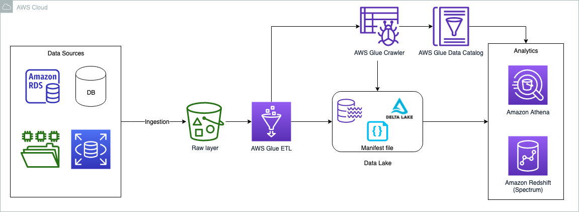
Handle UPSERT data operations using open-source Delta Lake and AWS Glue

Post Syndicated from Praveen Allam original https://aws.amazon.com/blogs/big-data/handle-upsert-data-operations-using-open-source-delta-lake-and-aws-glue/

Many customers need an ACID transaction (atomic, consistent, isolated, durable) data lake that can log change data capture (CDC) from operational data sources. There is also demand for merging real-time data into batch data. Delta Lake framework provides these two capabilities. In this post, we discuss how to handle UPSERTs (updates and inserts) of the operational data using natively integrated Delta Lake with AWS Glue, and query the Delta Lake using Amazon Athena.

We examine a hypothetical insurance organization that issues commercial policies to small- and medium-scale businesses. The insurance prices vary based on several criteria, such as where the business is located, business type, earthquake or flood coverage, and so on. This organization is planning to build a data analytical platform, and the insurance policy data is one of the inputs to this platform. Because the business is growing, hundreds and thousands of new insurance policies are being enrolled and renewed every month. Therefore, all this operational data needs to be sent to Delta Lake in near-real time so that the organization can perform various analytics, and build machine learning (ML) models to serve their customers in a more efficient and cost-effective way.

Solution overview

The data can originate from any source, but typically customers want to bring operational data to data lakes to perform data analytics. One of the solutions is to bring the relational data by using AWS Database Migration Service (AWS DMS). AWS DMS tasks can be configured to copy the full load as well as ongoing changes (CDC). The full load and CDC load can be brought into the raw and curated (Delta Lake) storage layers in the data lake. To keep it simple, in this post we opt out of the data sources and ingestion layer; the assumption is that the data is already copied to the raw bucket in the form of CSV files. An AWS Glue ETL job does the necessary transformation and copies the data to the Delta Lake layer. The Delta Lake layer ensures ACID compliance of the source data.

The following diagram illustrates the solution architecture.
Architecture diagram

The use case we use in this post is about a commercial insurance company. We use a simple dataset that contains the following columns:

  • Policy – Policy number, entered as text
  • Expiry – Date that policy expires
  • Location – Location type (Urban or Rural)
  • State – Name of state where property is located
  • Region – Geographic region where property is located
  • Insured Value – Property value
  • Business Type – Business use type for property, such as Farming or Retail
  • Earthquake – Is earthquake coverage included (Y or N)
  • Flood – Is flood coverage included (Y or N)

The dataset contains a sample of 25 insurance policies. In the case of a production dataset, it may contain millions of records.

policy_id,expiry_date,location_name,state_code,region_name,insured_value,business_type,earthquake,flood
200242,2023-01-02,Urban,NY,East,1617630,Retail,N,N
200314,2023-01-02,Urban,NY,East,8678500,Apartment,Y,Y
200359,2023-01-02,Rural,WI,Midwest,2052660,Farming,N,N
200315,2023-01-02,Urban,NY,East,17580000,Apartment,Y,Y
200385,2023-01-02,Urban,NY,East,1925000,Hospitality,N,N
200388,2023-01-04,Urban,IL,Midwest,12934500,Apartment,Y,Y
200358,2023-01-05,Urban,WI,Midwest,928300,Office Bldg,N,N
200264,2023-01-07,Rural,NY,East,2219900,Farming,N,N
200265,2023-01-07,Urban,NY,East,14100000,Apartment,Y,Y
100582,2023-03-25,Urban,NJ,East,4651680,Apartment,Y,Y
100487,2023-03-25,Urban,NY,East,5990067,Apartment,N,N
100519,2023-03-25,Rural,NY,East,4102500,Farming,N,N
100462,2023-03-25,Urban,NY,East,3400000,Construction,Y,Y
100486,2023-03-26,Urban,NY,East,9973900,Apartment,Y,Y
100463,2023-03-27,Urban,NY,East,15480000,Office Bldg,Y,Y
100595,2023-03-27,Rural,NY,East,2446600,Farming,N,N
100617,2023-03-27,Urban,VT,Northeast,8861500,Office Bldg,N,N
100580,2023-03-30,Urban,NH,Northeast,97920,Office Bldg,Y,Y
100581,2023-03-30,Urban,NY,East,5150000,Apartment,Y,Y
100475,2023-03-31,Rural,WI,Midwest,1451662,Farming,N,N
100503,2023-03-31,Urban,NJ,East,1761960,Office Bldg,N,N
100504,2023-03-31,Rural,NY,East,1649105,Farming,N,N
100616,2023-03-31,Urban,NY,East,2329500,Apartment,N,N
100611,2023-04-25,Urban,NJ,East,1595500,Office Bldg,Y,Y
100621,2023-04-25,Urban,MI,Central,394220,Retail,N,N

In the following sections, we walk through the steps to perform the Delta Lake UPSERT operations. We use the AWS Management Console to perform all the steps. However, you can also automate these steps using tools like AWS CloudFormation, the AWS Cloud Development Kit (AWS CDK), Terraforms, and so on.

Prerequisites

This post is focused towards architects, engineers, developers, and data scientists who build, design, and build analytical solutions on AWS. We expect a basic understanding of the console, AWS Glue, Amazon Simple Storage Service (Amazon S3), and Athena. Additionally, the persona is able to create AWS Identity and Access Management (IAM) policies and roles, create and run AWS Glue jobs and crawlers, and is able work with the Athena query editor.

Use Athena query engine version 3 to query delta lake tables, later in the section “Query the full load using Athena”.

Athena QE V3

Set up an S3 bucket for full and CDC load data feeds

To set up your S3 bucket, complete the following steps:

  1. Log in to your AWS account and choose a Region nearest to you.
  2. On the Amazon S3 console, create a new bucket. Make sure the name is unique (for example, delta-lake-cdc-blog-<some random number>).
  3. Create the following folders:
    1. $bucket_name/fullload – This folder is used for a one-time full load from the upstream data source
    2. $bucket_name/cdcload – This folder is used for copying the upstream data changes
    3. $bucket_name/delta – This folder holds the Delta Lake data files
  4. Copy the sample dataset and save it in a file called full-load.csv to your local machine.
  5. Upload the file using the Amazon S3 console into the folder $bucket_name/fullload.

s3 folders

Set up an IAM policy and role

In this section, we create an IAM policy for the S3 bucket access and a role for AWS Glue jobs to run, and also use the same role for querying the Delta Lake using Athena.

  1. On the IAM console, choose Polices in the navigation pane.
  2. Choose Create policy.
  3. Select JSON tab and paste the following policy code. Replace the {bucket_name} you created in the earlier step.
{
    "Version": "2012-10-17",
    "Statement": [
        {
            "Sid": "AllowListingOfFolders",
            "Action": [
                "s3:ListBucket",
                "s3:GetBucketLocation"
            ],
            "Effect": "Allow",
            "Resource": [
                "arn:aws:s3:::{bucket_name}"
            ]
        },
        {
            "Sid": "ObjectAccessInBucket",
            "Effect": "Allow",
            "Action": [
                "s3:PutObject",
                "s3:GetObject",
                "s3:DeleteObject"
            ],
            "Resource": "arn:aws:s3:::{bucket_name}/*"
        }
    ]
}
  1. Name the policy delta-lake-cdc-blog-policy and select Create policy.
  2. On the IAM console, choose Roles in the navigation pane.
  3. Choose Create role.
  4. Select AWS Glue as your trusted entity and choose Next.
  5. Select the policy you just created, and with two additional AWS managed policies:
    1. delta-lake-cdc-blog-policy
    2. AWSGlueServiceRole
    3. CloudWatchFullAccess
  1. Choose Next.
  2. Give the role a name (for example, delta-lake-cdc-blog-role).

IAM role

Set up AWS Glue jobs

In this section, we set up two AWS Glue jobs: one for full load and one for the CDC load. Let’s start with the full load job.

  1. On the AWS Glue console, under Data Integration and ETL in the navigation pane, choose Jobs. AWS Glue Studio opens in a new tab.
  2. Select Spark script editor and choose Create.

Glue Studio Editor

  1. In the script editor, replace the code with the following code snippet
import sys
from awsglue.utils import getResolvedOptions
from pyspark.sql.session import SparkSession
from pyspark.sql.types import *

## @params: [JOB_NAME]
args = getResolvedOptions(sys.argv, ['JOB_NAME','s3_bucket'])

# Initialize Spark Session with Delta Lake
spark = SparkSession \
.builder \
.config("spark.sql.extensions", "io.delta.sql.DeltaSparkSessionExtension") \
.config("spark.sql.catalog.spark_catalog", "org.apache.spark.sql.delta.catalog.DeltaCatalog") \
.getOrCreate()

#Define the table schema
schema = StructType() \
      .add("policy_id",IntegerType(),True) \
      .add("expiry_date",DateType(),True) \
      .add("location_name",StringType(),True) \
      .add("state_code",StringType(),True) \
      .add("region_name",StringType(),True) \
      .add("insured_value",IntegerType(),True) \
      .add("business_type",StringType(),True) \
      .add("earthquake_coverage",StringType(),True) \
      .add("flood_coverage",StringType(),True) 

# Read the full load
sdf = spark.read.format("csv").option("header",True).schema(schema).load("s3://"+ args['s3_bucket']+"/fullload/")
sdf.printSchema()

# Write data as DELTA TABLE
sdf.write.format("delta").mode("overwrite").save("s3://"+ args['s3_bucket']+"/delta/insurance/")
  1. Navigate to the Job details tab.
  2. Provide a name for the job (for example, Full-Load-Job).
  3. For IAM Role¸ choose the role delta-lake-cdc-blog-role that you created earlier.
  4. For Worker type¸ choose G 2X.
  5. For Job bookmark, choose Disable.
  6. Set Number of retries to 0.
  7. Under Advanced properties¸ keep the default values, but provide the delta core JAR file path for Python library path and Dependent JARs path.
  8. Under Job parameters:
    1. Add the key --s3_bucket with the bucket name you created earlier as the value.
    2. Add the key --datalake-formats  and give the value delta
  9. Keep the remaining default values and choose Save.

Job details

Now let’s create the CDC load job.

  1. Create a second job called CDC-Load-Job.
  2. Follow the steps on the Job details tab as with the previous job.
  3. Alternatively, you may choose “Clone job” option from the Full-Load-Job, this will carry all the job details from the full load job.
  4. In the script editor, enter the following code snippet for the CDC logic:
import sys
from awsglue.utils import getResolvedOptions
from awsglue.context import GlueContext
from pyspark.sql.session import SparkSession
from pyspark.sql.functions import col
from pyspark.sql.functions import expr

## For Delta lake
from delta.tables import DeltaTable


## @params: [JOB_NAME]
args = getResolvedOptions(sys.argv, ['JOB_NAME','s3_bucket'])

# Initialize Spark Session with Delta Lake
spark = SparkSession \
.builder \
.config("spark.sql.extensions", "io.delta.sql.DeltaSparkSessionExtension") \
.config("spark.sql.catalog.spark_catalog", "org.apache.spark.sql.delta.catalog.DeltaCatalog") \
.getOrCreate()

# Read the CDC load
cdc_df = spark.read.csv("s3://"+ args['s3_bucket']+"/cdcload")
cdc_df.show(5,True)

# now read the full load (latest data) as delta table
delta_df = DeltaTable.forPath(spark, "s3://"+ args['s3_bucket']+"/delta/insurance/")
delta_df.toDF().show(5,True)

# UPSERT process if matches on the condition the update else insert
# if there is no keyword then create a data set with Insert, Update and Delete flag and do it separately.
# for delete it has to run in loop with delete condition, this script do not handle deletes.
    
final_df = delta_df.alias("prev_df").merge( \
source = cdc_df.alias("append_df"), \
#matching on primarykey
condition = expr("prev_df.policy_id = append_df._c1"))\
.whenMatchedUpdate(set= {
    "prev_df.expiry_date"           : col("append_df._c2"), 
    "prev_df.location_name"         : col("append_df._c3"),
    "prev_df.state_code"            : col("append_df._c4"),
    "prev_df.region_name"           : col("append_df._c5"), 
    "prev_df.insured_value"         : col("append_df._c6"),
    "prev_df.business_type"         : col("append_df._c7"),
    "prev_df.earthquake_coverage"   : col("append_df._c8"), 
    "prev_df.flood_coverage"        : col("append_df._c9")} )\
.whenNotMatchedInsert(values =
#inserting a new row to Delta table
{   "prev_df.policy_id"             : col("append_df._c1"),
    "prev_df.expiry_date"           : col("append_df._c2"), 
    "prev_df.location_name"         : col("append_df._c3"),
    "prev_df.state_code"            : col("append_df._c4"),
    "prev_df.region_name"           : col("append_df._c5"), 
    "prev_df.insured_value"         : col("append_df._c6"),
    "prev_df.business_type"         : col("append_df._c7"),
    "prev_df.earthquake_coverage"   : col("append_df._c8"), 
    "prev_df.flood_coverage"        : col("append_df._c9")
})\
.execute()

Run the full load job

On the AWS Glue console, open full-load-job and choose Run. The job takes about 2 minutes to complete, and the job run status changes to Succeeded. Go to $bucket_name and open the delta folder, which contains the insurance folder. You can note the Delta Lake files in it. Delta location on S3

Create and run the AWS Glue crawler

In this step, we create an AWS Glue crawler with Delta Lake as the data source type. After successfully running the crawler, we inspect the data using Athena.

  1. On the AWS Glue console, choose Crawlers in the navigation pane.
  2. Choose Create crawler.
  3. Provide a name (for example, delta-lake-crawler) and choose Next.
  4. Choose Add a data source and choose Delta Lake as your data source.
  5. Copy your delta folder URI (for example, s3://delta-lake-cdc-blog-123456789/delta/insurance) and enter the Delta Lake table path location.
  6. Keep the default selection Create Native tables, and choose Add a Delta Lake data source.
  7. Choose Next.
  8. Choose the IAM role you created earlier, then choose Next.
  9. Select the default target database, and provide delta_ for the table name prefix. If no default database exist, you may create one.
  10. Choose Next.
  11. Choose Create crawler.
  12. Run the newly created crawler. After the crawler is complete, the delta_insurance table is available under Databases/Tables.
  13. Open the table to check the table overview.

You can observe nine columns and their data types. Glue table

Query the full load using Athena

In the earlier step, we created the delta_insurance table by running a crawler against the Delta Lake location. In this section, we query the delta_insurance table using Athena. Note that if you’re using Athena for the first time, set the query output folder to store the Athena query results (for example, s3://<your-s3-bucket>/query-output/).

  1. On the Athena console, open the query editor.
  2. Keep the default selections for Data source and Database.
  3. Run the query SELECT * FROM delta_insurance;. This query returns a total of 25 rows, the same as what was in the full load data feed.
  4. For the CDC comparison, run the following query and store the results in a location where you can compare these results later:
SELECT * FROM delta_insurance
WHERE policy_id IN (100462,100463,100475,110001,110002)
order by policy_id;

The following screenshot shows the Athena query result.

Query results from full load

Upload the CDC data feed and run the CDC job

In this section, we update three insurance policies and insert two new policies.

  1. Copy the following insurance policy data and save it locally as cdc-load.csv:
U,100462,2024-12-31,Urban,NY,East,3400000,Construction,Y,Y
U,100463,2023-03-27,Urban,NY,East,1000000,Office Bldg,Y,Y
U,100475,2023-03-31,Rural,WI,Midwest,1451662,Farming,N,Y
I,110001,2024-03-31,Urban,CA,WEST,210000,Office Bldg,N,N
I,110002,2024-03-31,Rural,FL,East,975000,Retail,N,Y

The first column in the CDC feed describes the UPSERT operations. U is for updating an existing record, and I is for inserting a new record.

  1. Upload the cdc-load.csv file to the $bucket_name/cdcload/ folder.
  2. On the AWS Glue console, run CDC-Load-Job. This job takes care of updating the Delta Lake accordingly.

The change details are as follows:

  • 100462 – Expiry date changes to 12/31/2024
  • 100463 – Insured value changes to 1 million
  • 100475 – This policy is now under a new flood zone
  • 110001 and 110002 – New policies added to the table
  1. Run the query again:
SELECT * FROM delta_insurance
WHERE policy_id IN (100462, 100463,100475,110001,110002)
order by policy_id;

As shown in the following screenshot, the changes in the CDC data feed are reflected in the Athena query results.
Athena query results

Clean up

In this solution, we used all managed services, and there is no cost if AWS Glue jobs aren’t running. However, if you want to clean up the tasks, you can delete the two AWS Glue jobs, AWS Glue table, and S3 bucket.

Conclusion

Organizations are continuously looking at high performance, cost-effective, and scalable analytical solutions to extract the value of their operational data sources in near-real time. The analytical platform should be ready to receive changes in the operational data as soon as they occur. Typical data lake solutions face challenges to handle the changes in source data; the Delta Lake framework can close this gap. This post demonstrated how to build data lakes for UPSERT operations using AWS Glue and native Delta Lake tables, and how to query AWS Glue tables from Athena. You can implement your large scale UPSERT data operations using AWS Glue, Delta Lake and perform analytics using Amazon Athena.

References


About the Authors

 Praveen Allam is a Solutions Architect at AWS. He helps customers design scalable, better cost-perfromant enterprise-grade applications using the AWS Cloud. He builds solutions to help organizations make data-driven decisions.

Vivek Singh is Senior Solutions Architect with the AWS Data Lab team. He helps customers unblock their data journey on the AWS ecosystem. His interest areas are data pipeline automation, data quality and data governance, data lakes, and lake house architectures.
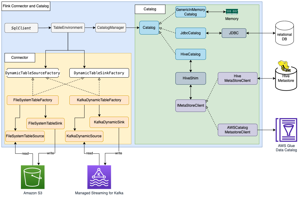
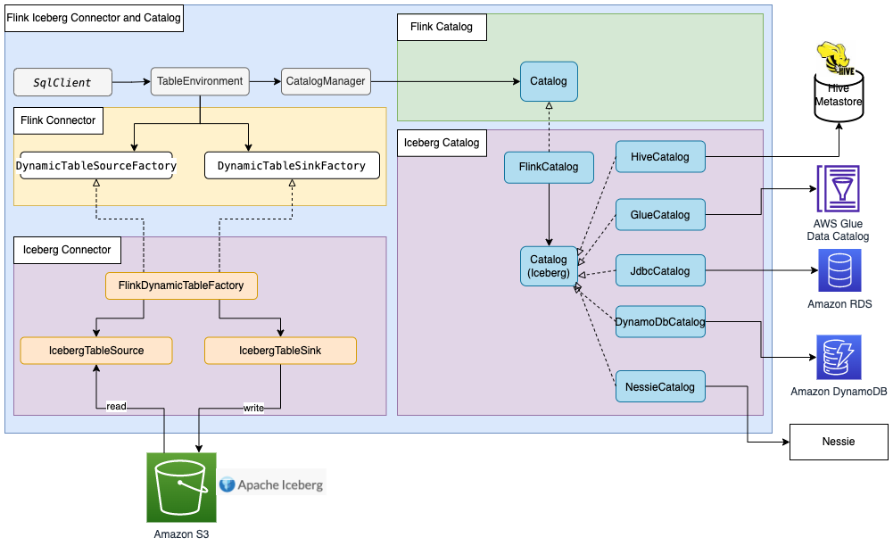
Build a data lake with Apache Flink on Amazon EMR

Post Syndicated from Jianwei Li original https://aws.amazon.com/blogs/big-data/build-a-unified-data-lake-with-apache-flink-on-amazon-emr/

To build a data-driven business, it is important to democratize enterprise data assets in a data catalog. With a unified data catalog, you can quickly search datasets and figure out data schema, data format, and location. The AWS Glue Data Catalog provides a uniform repository where disparate systems can store and find metadata to keep track of data in data silos.

Apache Flink is a widely used data processing engine for scalable streaming ETL, analytics, and event-driven applications. It provides precise time and state management with fault tolerance. Flink can process bounded stream (batch) and unbounded stream (stream) with a unified API or application. After data is processed with Apache Flink, downstream applications can access the curated data with a unified data catalog. With unified metadata, both data processing and data consuming applications can access the tables using the same metadata.

This post shows you how to integrate Apache Flink in Amazon EMR with the AWS Glue Data Catalog so that you can ingest streaming data in real time and access the data in near-real time for business analysis.

Apache Flink connector and catalog architecture

Apache Flink uses a connector and catalog to interact with data and metadata. The following diagram shows the architecture of the Apache Flink connector for data read/write, and catalog for metadata read/write.

Flink Glue Architecture

For data read/write, Flink has the interface DynamicTableSourceFactory for read and DynamicTableSinkFactory for write. A different Flink connector implements two interfaces to access data in different storage. For example, the Flink FileSystem connector has FileSystemTableFactory to read/write data in Hadoop Distributed File System (HDFS) or Amazon Simple Storage Service (Amazon S3), the Flink HBase connector has HBase2DynamicTableFactory to read/write data in HBase, and the Flink Kafka connector has KafkaDynamicTableFactory to read/write data in Kafka. You can refer to Table & SQL Connectors for more information.

For metadata read/write, Flink has the catalog interface. Flink has three built-in implementations for the catalog. GenericInMemoryCatalog stores the catalog data in memory. JdbcCatalog stores the catalog data in a JDBC-supported relational database. As of this writing, MySQL and PostgreSQL databases are supported in the JDBC catalog. HiveCatalog stores the catalog data in Hive Metastore. HiveCatalog uses HiveShim to provide different Hive version compatibility. We can configure different metastore clients to use Hive Metastore or the AWS Glue Data Catalog. In this post, we configure the Amazon EMR property hive.metastore.client.factory.class to com.amazonaws.glue.catalog.metastore.AWSGlueDataCatalogHiveClientFactory (see Using the AWS Glue Data Catalog as the metastore for Hive) so that we can use the AWS Glue Data Catalog to store Flink catalog data. Refer to Catalogs for more information.

Most Flink built-in connectors, such as for Kafka, Amazon Kinesis, Amazon DynamoDB, Elasticsearch, or FileSystem, can use Flink HiveCatalog to store metadata in the AWS Glue Data Catalog. However, some connector implementations such as Apache Iceberg have their own catalog management mechanism. FlinkCatalog in Iceberg implements the catalog interface in Flink. FlinkCatalog in Iceberg has a wrapper to its own catalog implementation. The following diagram shows the relationship between Apache Flink, the Iceberg connector, and the catalog. For more information, refer to Creating catalogs and using catalogs and Catalogs.

Flink Iceberg Glue Architecture

Apache Hudi also has its own catalog management. Both HoodieCatalog and HoodieHiveCatalog implements a catalog interface in Flink. HoodieCatalog stores metadata in a file system such as HDFS. HoodieHiveCatalog stores metadata in Hive Metastore or the AWS Glue Data Catalog, depending on whether you configure hive.metastore.client.factory.class to use com.amazonaws.glue.catalog.metastore.AWSGlueDataCatalogHiveClientFactory. The following diagram shows relationship between Apache Flink, the Hudi connector, and the catalog. For more information, refer to Create Catalog.

Flink Hudi Glue Architecture

Because Iceberg and Hudi have different catalog management mechanisms, we show three scenarios of Flink integration with the AWS Glue Data Catalog in this post:

  • Read/Write to Iceberg tables in Flink with metadata in Glue Data Catalog
  • Read/Write to Hudi tables in Flink with metadata in Glue Data Catalog
  • Read/Write to other storage format in Flink with metadata in Glue Data Catalog

Solution overview

The following diagram shows the overall architecture of the solution described in this post.

Flink Glue Integration

In this solution, we enable an Amazon RDS for MySQL binlog to extract transaction changes in real time. The Amazon EMR Flink CDC connector reads the binlog data and processes the data. Transformed data can be stored in Amazon S3. We use the AWS Glue Data Catalog to store the metadata such as table schema and table location. Downstream data consumer applications such as Amazon Athena or Amazon EMR Trino access the data for business analysis.

The following are the high-level steps to set up this solution:

  1. Enable binlog for Amazon RDS for MySQL and initialize the database.
  2. Create an EMR cluster with the AWS Glue Data Catalog.
  3. Ingest change data capture (CDC) data with Apache Flink CDC in Amazon EMR.
  4. Store the processed data in Amazon S3 with metadata in the AWS Glue Data Catalog.
  5. Verify all table metadata is stored in the AWS Glue Data Catalog.
  6. Consume data with Athena or Amazon EMR Trino for business analysis.
  7. Update and delete source records in Amazon RDS for MySQL and validate the reflection of the data lake tables.

Prerequisites

This post uses an AWS Identity and Access Management (IAM) role with permissions for the following services:

  • Amazon RDS for MySQL (5.7.40)
  • Amazon EMR (6.9.0)
  • Amazon Athena
  • AWS Glue Data Catalog
  • Amazon S3

Enable binlog for Amazon RDS for MySQL and initialize the database

To enable CDC in Amazon RDS for MySQL, we need to configure binary logging for Amazon RDS for MySQL. Refer to Configuring MySQL binary logging for more information. We also create the database salesdb in MySQL and create the tables customer, order, and others to set up the data source.

  1. On the Amazon RDS console, choose Parameter groups in the navigation pane.
  2. Create a new parameter group for MySQL.
  3. Edit the parameter group you just created to set binlog_format=ROW.

RDS-Binlog-Format

  1. Edit the parameter group you just created to set binlog_row_image=full.

RDS-Binlog-Row-Image

  1. Create an RDS for MySQL DB instance with the parameter group.
  2. Note down the values for hostname, username, and password, which we use later.
  3. Download the MySQL database initialization script from Amazon S3 by running the following command:
aws s3 cp s3://emr-workshops-us-west-2/glue_immersion_day/scripts/salesdb.sql ./salesdb.sql
  1. Connect to the RDS for MySQL database and run the salesdb.sql command to initialize the database, providing the host name and user name according to your RDS for MySQL database configuration:
mysql -h <hostname> -u <username> -p
mysql> source salesdb.sql

Create an EMR cluster with the AWS Glue Data Catalog

From Amazon EMR 6.9.0, the Flink table API/SQL can integrate with the AWS Glue Data Catalog. To use the Flink and AWS Glue integration, you must create an Amazon EMR 6.9.0 or later version.

  1. Create the file iceberg.properties for the Amazon EMR Trino integration with the Data Catalog. When the table format is Iceberg, your file should have following content:
iceberg.catalog.type=glue
connector.name=iceberg
  1. Upload iceberg.properties to an S3 bucket, for example DOC-EXAMPLE-BUCKET.

For more information on how to integrate Amazon EMR Trino with Iceberg, refer to Use an Iceberg cluster with Trino.

  1. Create the file trino-glue-catalog-setup.sh to configure the Trino integration with the Data Catalog. Use trino-glue-catalog-setup.sh as the bootstrap script. Your file should have the following content (replace DOC-EXAMPLE-BUCKET with your S3 bucket name):
set -ex 
sudo aws s3 cp s3://DOC-EXAMPLE-BUCKET/iceberg.properties /etc/trino/conf/catalog/iceberg.properties

  1. Upload trino-glue-catalog-setup.sh to your S3 bucket (DOC-EXAMPLE-BUCKET).

Refer to Create bootstrap actions to install additional software to run a bootstrap script.

  1. Create the file flink-glue-catalog-setup.sh to configure the Flink integration with the Data Catalog.
  2. Use a script runner and run the flink-glue-catalog-setup.sh script as a step function.

Your file should have the following content (the JAR file name here is using Amazon EMR 6.9.0; a later version JAR name may change, so make sure to update according to your Amazon EMR version).

Note that here we use an Amazon EMR step, not a bootstrap, to run this script. An Amazon EMR step script is run after Amazon EMR Flink is provisioned.

set -ex

sudo cp /usr/lib/hive/auxlib/aws-glue-datacatalog-hive3-client.jar /usr/lib/flink/lib
sudo cp /usr/lib/hive/lib/antlr-runtime-3.5.2.jar /usr/lib/flink/lib
sudo cp /usr/lib/hive/lib/hive-exec.jar /lib/flink/lib
sudo cp /usr/lib/hive/lib/libfb303-0.9.3.jar /lib/flink/lib
sudo cp /usr/lib/flink/opt/flink-connector-hive_2.12-1.15.2.jar /lib/flink/lib
sudo chmod 755 /usr/lib/flink/lib/aws-glue-datacatalog-hive3-client.jar
sudo chmod 755 /usr/lib/flink/lib/antlr-runtime-3.5.2.jar
sudo chmod 755 /usr/lib/flink/lib/hive-exec.jar
sudo chmod 755 /usr/lib/flink/lib/libfb303-0.9.3.jar
sudo chmod 755 /usr/lib/flink/lib/flink-connector-hive_2.12-1.15.2.jar

sudo wget https://repo1.maven.org/maven2/com/ververica/flink-sql-connector-mysql-cdc/2.2.1/flink-sql-connector-mysql-cdc-2.2.1.jar -O /lib/flink/lib/flink-sql-connector-mysql-cdc-2.2.1.jar
sudo chmod 755 /lib/flink/lib/flink-sql-connector-mysql-cdc-2.2.1.jar

sudo ln -s /usr/share/aws/iceberg/lib/iceberg-flink-runtime.jar /usr/lib/flink/lib/
sudo ln -s /usr/lib/hudi/hudi-flink-bundle.jar /usr/lib/flink/lib/

sudo mv /usr/lib/flink/opt/flink-table-planner_2.12-1.15.2.jar /usr/lib/flink/lib/
sudo mv /usr/lib/flink/lib/flink-table-planner-loader-1.15.2.jar /usr/lib/flink/opt/
  1. Upload flink-glue-catalog-setup.sh to your S3 bucket (DOC-EXAMPLE-BUCKET).

Refer to Configuring Flink to Hive Metastore in Amazon EMR for more information on how to configure Flink and Hive Metastore. Refer to Run commands and scripts on an Amazon EMR cluster for more details on running the Amazon EMR step script.

  1. Create an EMR 6.9.0 cluster with the applications Hive, Flink, and Trino.

You can create an EMR cluster with the AWS Command Line Interface (AWS CLI) or the AWS Management Console. Refer to the appropriate subsection for instructions.

Create an EMR cluster with the AWS CLI

To use the AWS CLI, complete the following steps:

  1. Create the file emr-flink-trino-glue.json to configure Amazon EMR to use the Data Catalog. Your file should have the following content:
[
{
"Classification": "hive-site",
"Properties": {
"hive.metastore.client.factory.class": "com.amazonaws.glue.catalog.metastore.AWSGlueDataCatalogHiveClientFactory"
}
},
{
"Classification": "trino-connector-hive",
"Properties": {
"hive.metastore": "glue"
}
}
]
  1. Run the following command to create the EMR cluster. Provide your local emr-flink-trino-glue.json parent folder path, S3 bucket, EMR cluster Region, EC2 key name, and S3 bucket for EMR logs.
aws emr create-cluster --release-label emr-6.9.0 \
--applications Name=Hive Name=Flink Name=Spark Name=Trino \
--region us-west-2 \
--name flink-trino-glue-emr69 \
--configurations "file:///<your configuration path>/emr-flink-trino-glue.json" \
--bootstrap-actions '[{"Path":"s3://DOC-EXAMPLE-BUCKET/trino-glue-catalog-setup.sh","Name":"Add iceberg.properties for Trino"}]' \
--steps '[{"Args":["s3://DOC-EXAMPLE-BUCKET/flink-glue-catalog-setup.sh"],"Type":"CUSTOM_JAR","ActionOnFailure":"CONTINUE","Jar":"s3://<region>.elasticmapreduce/libs/script-runner/script-runner.jar","Properties":"","Name":"Flink-glue-integration"}]' \
--instance-groups \
InstanceGroupType=MASTER,InstanceType=m6g.2xlarge,InstanceCount=1 \
InstanceGroupType=CORE,InstanceType=m6g.2xlarge,InstanceCount=2 \
--use-default-roles \
--ebs-root-volume-size 30 \
--ec2-attributes KeyName=<keyname> \
--log-uri s3://<s3-bucket-for-emr>/elasticmapreduce/

Create an EMR cluster on the console

To use the console, complete the following steps:

  1. On the Amazon EMR console, create an EMR cluster and select Use for Hive table metadata for AWS Glue Data Catalog settings.
  2. Add configuration settings with the following code:
[
{
"Classification": "trino-connector-hive",
"Properties": {
"hive.metastore": "glue"
}
}
]

EMR-6.9-Flink-Hive-Glue-1

  1. In the Steps section, add a step called Custom JAR.
  2. Set JAR location to s3://<region>.elasticmapreduce/libs/script-runner/script-runner.jar, where <region> is the region in which your EMR cluster resides.
  3. Set Arguments to the S3 path you uploaded earlier.

EMR-6.9-Flink-Hive-Glue-2

  1. In the Bootstrap Actions section, choose Custom Action.
  2. Set Script location to the S3 path you uploaded.

EMR-6.9-Flink-Hive-Glue-3

  1. Continue the subsequent steps to complete your EMR cluster creation.

Ingest CDC data with Apache Flink CDC in Amazon EMR

The Flink CDC connector supports reading database snapshots and captures updates in the configured tables. We have deployed the Flink CDC connector for MySQL by downloading flink-sql-connector-mysql-cdc-2.2.1.jar and putting it into the Flink library when we create our EMR cluster. The Flink CDC connector can use the Flink Hive catalog to store Flink CDC table schema into Hive Metastore or the AWS Glue Data Catalog. In this post, we use the Data Catalog to store our Flink CDC table.

Complete the following steps to ingest RDS for MySQL databases and tables with Flink CDC and store metadata in the Data Catalog:

  1. SSH to the EMR primary node.
  2. Start Flink on a YARN session by running the following command, providing your S3 bucket name:
flink-yarn-session -d -jm 2048 -tm 4096 -s 2 \
-D state.backend=rocksdb \
-D state.backend.incremental=true \
-D state.checkpoint-storage=filesystem \
-D state.checkpoints.dir=s3://<flink-glue-integration-bucket>/flink-checkponts/ \
-D state.checkpoints.num-retained=10 \
-D execution.checkpointing.interval=10s \
-D execution.checkpointing.mode=EXACTLY_ONCE \
-D execution.checkpointing.externalized-checkpoint-retention=RETAIN_ON_CANCELLATION \
-D execution.checkpointing.max-concurrent-checkpoints=1
  1. Start the Flink SQL client CLI by running the following command:
/usr/lib/flink/bin/sql-client.sh embedded
  1. Create the Flink Hive catalog by specifying the catalog type as hive and providing your S3 bucket name:
CREATE CATALOG glue_catalog WITH (
'type' = 'hive',
'default-database' = 'default',
'hive-conf-dir' = '/etc/hive/conf.dist'
);
USE CATALOG glue_catalog;
CREATE DATABASE IF NOT EXISTS flink_cdc_db WITH ('hive.database.location-uri'= 's3://<flink-glue-integration-bucket>/flink-glue-for-hive/warehouse/')
use flink_cdc_db;

Because we’re configuring the EMR Hive catalog use the AWS Glue Data Catalog, all the databases and tables created in the Flink Hive catalog are stored in the Data Catalog.

  1. Create the Flink CDC table, providing the host name, user name, and password for the RDS for MySQL instance you created earlier.

Note that because the RDS for MySQL user name and password will be stored in the Data Catalog as table properties, you should be enable AWS Glue database/table authorization with AWS Lake Formation to protect your sensitive data.

CREATE TABLE `glue_catalog`.`flink_cdc_db`.`customer_cdc` (
`CUST_ID` double NOT NULL,
`NAME` STRING NOT NULL,
`MKTSEGMENT` STRING NOT NULL,
PRIMARY KEY (`CUST_ID`) NOT ENFORCED
) WITH (
'connector' = 'mysql-cdc',
'hostname' = '<hostname>',
'port' = '3306',
'username' = '<username>',
'password' = '<password>',
'database-name' = 'salesdb',
'table-name' = 'CUSTOMER'
);

CREATE TABLE `glue_catalog`.`flink_cdc_db`.`customer_site_cdc` (
`SITE_ID` double NOT NULL,
`CUST_ID` double NOT NULL,
`ADDRESS` STRING NOT NULL,
`CITY` STRING NOT NULL,
`STATE` STRING NOT NULL,
`COUNTRY` STRING NOT NULL,
`PHONE` STRING NOT NULL,
PRIMARY KEY (`SITE_ID`) NOT ENFORCED
) WITH (
'connector' = 'mysql-cdc',
'hostname' = '<hostname>',
'port' = '3306',
'username' = '<username>',
'password' = '<password>',
'database-name' = 'salesdb',
'table-name' = 'CUSTOMER_SITE'
);

CREATE TABLE `glue_catalog`.`flink_cdc_db`.`sales_order_all_cdc` (
`ORDER_ID` int NOT NULL,
`SITE_ID` double NOT NULL,
`ORDER_DATE` TIMESTAMP NOT NULL,
`SHIP_MODE` STRING NOT NULL
) WITH (
'connector' = 'mysql-cdc',
'hostname' = '<hostname>',
'port' = '3306',
'username' = '<username>',
'password' = '<password>',
'database-name' = 'salesdb',
'table-name' = 'SALES_ORDER_ALL',
'scan.incremental.snapshot.enabled' = 'FALSE'
);
  1. Query the table you just created:
SELECT count(O.ORDER_ID) AS ORDER_COUNT,
C.CUST_ID,
C.NAME,
C.MKTSEGMENT
FROM   customer_cdc C
JOIN customer_site_cdc CS
ON C.CUST_ID = CS.CUST_ID
JOIN sales_order_all_cdc O
ON O.SITE_ID = CS.SITE_ID
GROUP  BY C.CUST_ID,
C.NAME,
C.MKTSEGMENT;

You will get a query result like following screenshot.

Flink-SQL-CDC-Test

Store processed data in Amazon S3 with metadata in the Data Catalog

As we’re ingesting the relational database data in Amazon RDS for MySQL, raw data may be updated or deleted. To support data update and delete, we can choose data lake technologies such as Apache Iceberg or Apache Hudi to store the processed data. As we mentioned earlier, Iceberg and Hudi have different catalog management. We show both scenarios to use Flink to read/write the Iceberg and Hudi tables with metadata in the AWS Glue Data Catalog.

For non-Iceberg and non-Hudi, we use a FileSystem Parquet file to show how the Flink built-in connector uses the Data Catalog.

Read/Write to Iceberg tables in Flink with metadata in Glue Data Catalog

The following diagram shows the architecture for this configuration.

Flink Glue Integration for Iceberg

  1. Create a Flink Iceberg catalog using the Data Catalog by specifying catalog-impl as org.apache.iceberg.aws.glue.GlueCatalog.

For more information about Flink and Data Catalog integration for Iceberg, refer to Glue Catalog.

  1. In the Flink SQL client CLI, run the following command, providing your S3 bucket name:
CREATE CATALOG glue_catalog_for_iceberg WITH (
'type'='iceberg',
'warehouse'='s3://<flink-glue-integration-bucket>/flink-glue-for-iceberg/warehouse/',
'catalog-impl'='org.apache.iceberg.aws.glue.GlueCatalog',
'io-impl'='org.apache.iceberg.aws.s3.S3FileIO',
'lock-impl'='org.apache.iceberg.aws.glue.DynamoLockManager',
'lock.table'='FlinkGlue4IcebergLockTable' );
  1. Create an Iceberg table to store processed data:
USE CATALOG glue_catalog_for_iceberg;
CREATE DATABASE IF NOT EXISTS flink_glue_iceberg_db;
USE flink_glue_iceberg_db;
CREATE TABLE `glue_catalog_for_iceberg`.`flink_glue_iceberg_db`.`customer_summary` (
`CUSTOMER_ID` bigint,
`NAME` STRING,
`MKTSEGMENT` STRING,
`COUNTRY` STRING,
`ORDER_COUNT` BIGINT,
PRIMARY KEY (`CUSTOMER_ID`) NOT Enforced
)
WITH (
'format-version'='2',
'write.upsert.enabled'='true');
  1. Insert the processed data into Iceberg:
INSERT INTO `glue_catalog_for_iceberg`.`flink_glue_iceberg_db`.`customer_summary`
SELECT CAST(C.CUST_ID AS BIGINT) CUST_ID,
C.NAME,
C.MKTSEGMENT,
CS.COUNTRY,
count(O.ORDER_ID) AS ORDER_COUNT
FROM   `glue_catalog`.`flink_cdc_db`.`customer_cdc` C
JOIN `glue_catalog`.`flink_cdc_db`.`customer_site_cdc` CS
ON C.CUST_ID = CS.CUST_ID
JOIN `glue_catalog`.`flink_cdc_db`.`sales_order_all_cdc` O
ON O.SITE_ID = CS.SITE_ID
GROUP  BY C.CUST_ID,
C.NAME,
C.MKTSEGMENT,
CS.COUNTRY;

Read/Write to Hudi tables in Flink with metadata in Glue Data Catalog

The following diagram shows the architecture for this configuration.

Flink Glue Integration for Hudi

Complete the following steps:

  1. Create a catalog for Hudi to use the Hive catalog by specifying mode as hms.

Because we already configured Amazon EMR to use the Data Catalog when we created the EMR cluster, this Hudi Hive catalog uses the Data Catalog under the hood. For more information about Flink and Data Catalog integration for Hudi, refer to Create Catalog.

  1. In the Flink SQL client CLI, run the following command, providing your S3 bucket name:
CREATE CATALOG glue_catalog_for_hudi WITH (
'type' = 'hudi',
'mode' = 'hms',
'table.external' = 'true',
'default-database' = 'default',
'hive.conf.dir' = '/etc/hive/conf.dist',
'catalog.path' = 's3://<flink-glue-integration-bucket>/flink-glue-for-hudi/warehouse/'
);
  1. Create a Hudi table using the Data Catalog, and provide your S3 bucket name:
USE CATALOG glue_catalog_for_hudi;
CREATE DATABASE IF NOT EXISTS flink_glue_hudi_db;
use flink_glue_hudi_db;
CREATE TABLE `glue_catalog_for_hudi`.`flink_glue_hudi_db`.`customer_summary` (
`CUSTOMER_ID` bigint,
`NAME` STRING,
`MKTSEGMENT` STRING,
`COUNTRY` STRING,
`ORDER_COUNT` BIGINT,
PRIMARY KEY (`CUSTOMER_ID`) NOT Enforced
)
WITH (
'connector' = 'hudi',
'write.tasks' = '4',
'path' = 's3://<flink-glue-integration-bucket>/flink-glue-for-hudi/warehouse/customer_summary',
'table.type' = 'COPY_ON_WRITE',
'read.streaming.enabled' = 'true',
'read.streaming.check-interval' = '1'
);
  1. Insert the processed data into Hudi:
INSERT INTO `glue_catalog_for_hudi`.`flink_glue_hudi_db`.`customer_summary`
SELECT CAST(C.CUST_ID AS BIGINT) CUST_ID,
C.NAME,
C.MKTSEGMENT,
CS.COUNTRY,
count(O.ORDER_ID) AS ORDER_COUNT
FROM   `glue_catalog`.`flink_cdc_db`.`customer_cdc` C
JOIN `glue_catalog`.`flink_cdc_db`.`customer_site_cdc` CS
ON C.CUST_ID = CS.CUST_ID
JOIN `glue_catalog`.`flink_cdc_db`.`sales_order_all_cdc` O
ON O.SITE_ID = CS.SITE_ID
GROUP  BY C.CUST_ID,
C.NAME,
C.MKTSEGMENT,
CS.COUNTRY;

Read/Write to other storage format in Flink with metadata in Glue Data Catalog

The following diagram shows the architecture for this configuration.

Flink Glue Integration for Parquet

We already created the Flink Hive catalog in the previous step, so we’ll reuse that catalog.

  1. In the Flink SQL client CLI, run the following command:
USE CATALOG glue_catalog;
CREATE DATABASE IF NOT EXISTS flink_hive_parquet_db;
use flink_hive_parquet_db;

We change the SQL dialect to Hive to create a table with Hive syntax.

  1. Create a table with the following SQL, and provide your S3 bucket name:
SET table.sql-dialect=hive;

CREATE TABLE `customer_summary` (
`CUSTOMER_ID` bigint,
`NAME` STRING,
`MKTSEGMENT` STRING,
`COUNTRY` STRING,
`ORDER_COUNT` BIGINT
)
STORED AS parquet
LOCATION 's3://<flink-glue-integration-bucket>/flink-glue-for-hive-parquet/warehouse/customer_summary';

Because Parquet files don’t support updated rows, we can’t consume data from CDC data. However, we can consume data from Iceberg or Hudi.

  1. Use the following code to query the Iceberg table and insert data into the Parquet table:
SET table.sql-dialect=default;
SET execution.runtime-mode = batch;
INSERT INTO `glue_catalog`.`flink_hive_parquet_db`.`customer_summary`
SELECT * from `glue_catalog_for_iceberg`.`flink_glue_iceberg_db`.`customer_summary`;

Verify all table metadata is stored in the Data Catalog

You can navigate to the AWS Glue console to verify all the tables are stored in the Data Catalog.

  1. On the AWS Glue console, choose Databases in the navigation pane to list all the databases we created.

Glue-Databases

  1. Open a database and verify that all the tables are in that database.

Glue-Tables

Consume data with Athena or Amazon EMR Trino for business analysis

You can use Athena or Amazon EMR Trino to access the result data.

Query the data with Athena

To access the data with Athena, complete the following steps:

  1. Open the Athena query editor.
  2. Choose flink_glue_iceberg_db for Database.

You should see the customer_summary table listed.

  1. Run the following SQL script to query the Iceberg result table:
select * from customer_summary order by order_count desc limit 10

The query result will look like the following screenshot.

Athena-Iceberg-Query

  1. For the Hudi table, change Database to flink_glue_hudi_db and run the same SQL query.

Athena-Hudi-Query

  1. For the Parquet table, change Database to flink_hive_parquet_db and run the same SQL query.

Athena-Parquet-Query

Query the data with Amazon EMR Trino

To access Iceberg with Amazon EMR Trino, SSH to the EMR primary node.

  1. Run the following command to start the Trino CLI:
trino-cli --catalog iceberg

Amazon EMR Trino can now query the tables in the AWS Glue Data Catalog.

  1. Run the following command to query the result table:
show schemas;
use flink_glue_iceberg_db;
show tables;
select * from customer_summary order by order_count desc limit 10;

The query result looks like the following screenshot.

EMR-Trino-Iceberg-Query

  1. Exit the Trino CLI.
  2. Start the Trino CLI with the hive catalog to query the Hudi table:
trino-cli --catalog hive
  1. Run the following command to query the Hudi table:
show schemas;
use flink_glue_hudi_db;
show tables;
select * from customer_summary order by order_count desc limit 10;

Update and delete source records in Amazon RDS for MySQL and validate the reflection of the data lake tables

We can update and delete some records in the RDS for MySQL database and then validate that the changes are reflected in the Iceberg and Hudi tables.

  1. Connect to the RDS for MySQL database and run the following SQL:
update CUSTOMER set NAME = 'updated_name' where CUST_ID=7;

delete from CUSTOMER where CUST_ID=11;
  1. Query the customer_summary table with Athena or Amazon EMR Trino.

The updated and deleted records are reflected in the Iceberg and Hudi tables.

Athena-Iceberg-Query-Updated

Clean up

When you’re done with this exercise, complete the following steps to delete your resources and stop incurring costs:

  1. Delete the RDS for MySQL database.
  2. Delete the EMR cluster.
  3. Drop the databases and tables created in the Data Catalog.
  4. Remove files in Amazon S3.

Conclusion

This post showed you how to integrate Apache Flink in Amazon EMR with the AWS Glue Data Catalog. You can use a Flink SQL connector to read/write data in a different store, such as Kafka, CDC, HBase, Amazon S3, Iceberg, or Hudi. You can also store the metadata in the Data Catalog. The Flink table API has the same connector and catalog implementation mechanism. In a single session, we can use multiple catalog instances pointing to different types, like IcebergCatalog and HiveCatalog, and use then interchangeably in your query. You can also write code with the Flink table API to develop the same solution to integrate Flink and the Data Catalog.

In our solution, we consumed the RDS for MySQL binary log directly with Flink CDC. You can also use Amazon MSK Connect to consume the binary log with MySQL Debezim and store the data in Amazon Managed Streaming for Apache Kafka (Amazon MSK). Refer to Create a low-latency source-to-data lake pipeline using Amazon MSK Connect, Apache Flink, and Apache Hudi for more information.

With the Amazon EMR Flink unified batch and streaming data processing function, you can ingest and process data with one computing engine. With Apache Iceberg and Hudi integrated in Amazon EMR, you can build an evolvable and scalable data lake. With the AWS Glue Data Catalog, you can manage all enterprise data catalogs in a unified manner and consume data easily.

Follow the steps in this post to build your unified batch and streaming solution with Amazon EMR Flink and the AWS Glue Data Catalog. Please leave a comment if you have any questions.


About the Authors

Jianwei Li is Senior Analytics Specialist TAM. He provides consultant service for AWS enterprise support customers to design and build modern data platform.


Samrat Deb is Software Development Engineer at Amazon EMR. In his spare time, he love exploring new places, different culture and food.


Prabhu Josephraj is a Senior Software Development Engineer working for Amazon EMR. He is focused on leading the team that builds solutions in Apache Hadoop and Apache Flink. In his spare time, Prabhu enjoys spending time with his family.

Introducing native support for Apache Hudi, Delta Lake, and Apache Iceberg on AWS Glue for Apache Spark, Part 1: Getting Started

Post Syndicated from Akira Ajisaka original https://aws.amazon.com/blogs/big-data/part-1-getting-started-introducing-native-support-for-apache-hudi-delta-lake-and-apache-iceberg-on-aws-glue-for-apache-spark/

AWS Glue is a serverless, scalable data integration service that makes it easier to discover, prepare, move, and integrate data from multiple sources. AWS Glue provides an extensible architecture that enables users with different data processing use cases.

A common use case is building data lakes on Amazon Simple Storage Service (Amazon S3) using AWS Glue extract, transform, and load (ETL) jobs. Data lakes free you from proprietary data formats defined by the business intelligence (BI) tools and limited capacity of proprietary storage. In addition, data lakes help you break down data silos to maximize end-to-end data insights. As data lakes have grown in size and matured in usage, a significant amount of effort can be spent keeping the data up to date by ensuring files are updated in a transactionally consistent manner.

AWS Glue customers can now use the following open-source data lake storage frameworks: Apache Hudi, Linux Foundation Delta Lake, and Apache Iceberg. These data lake frameworks help you store data and interface data with your applications and frameworks. Although popular data file formats such as Apache Parquet, CSV, and JSON can store big data, data lake frameworks bundle distributed big data files into tabular structures that are otherwise hard to manage. This makes data lake table frameworks the building constructs of databases on data lakes.

We announced general availability for native support for Apache Hudi, Linux Foundation Delta Lake, and Apache Iceberg on AWS Glue for Spark. This feature removes the need to install a separate connector or associated dependencies, manage versions, and simplifies the configuration steps required to use these frameworks in AWS Glue for Apache Spark. With these open-source data lake frameworks, you can simplify incremental data processing in data lakes built on Amazon S3 by using ACID (atomicity, consistency, isolation, durability) transactions, upserts, and deletes.

This post demonstrates how AWS Glue for Apache Spark works with Hudi, Delta, and Iceberg dataset tables, and describes typical use cases on an AWS Glue Studio notebook.

Enable Hudi, Delta, Iceberg in Glue for Apache Spark

You can use Hudi, Delta, or Iceberg by specifying a new job parameter --datalake-formats. For example, if you want to use Hudi, you need to specify the key as --datalake-formats and the value as hudi. If the option is set, AWS Glue automatically adds the required JAR files into the runtime Java classpath, and that’s all you need. You don’t need to build and configure the required libraries or install a separate connector. You can use the following library versions with this option.

AWS Glue version Hudi Delta Lake Iceberg
AWS Glue 3.0 0.10.1 1.0.0 0.13.1
AWS Glue 4.0 0.12.1 2.1.0 1.0.0

If you want to use other versions of the preceding libraries, you can choose either of the following options:

If you choose either of the preceding options, you need to make sure the --datalake-formats job parameter is unspecified. For more information, see Process Apache Hudi, Delta Lake, Apache Iceberg datasets at scale, part 1: AWS Glue Studio Notebook.

Prerequisites

To continue this tutorial, you need to create the following AWS resources in advance:

Process Hudi, Delta, and Iceberg datasets on an AWS Glue Studio notebook

AWS Glue Studio notebooks provide serverless notebooks with minimal setup. It makes data engineers and developers quickly and interactively explore and process their datasets. You can start using Hudi, Delta, or Iceberg in an AWS Glue Studio notebook by specifying the parameter via %%configure magic and setting the AWS Glue version to 3.0 as follows:

# Use Glue version 3.0
%glue_version 3.0

# Configure '--datalake-formats' Job parameter
%%configure
{
  "--datalake-formats": "your_comma_separated_formats"
}

For more information, refer to the example notebooks available in the GitHub repository:

For this post, we use an Iceberg DataFrame as an example.

The following sections explain how to use an AWS Glue Studio notebook to create an Iceberg table and append records to the table.

Launch a Jupyter notebook to process Iceberg tables

Complete the following steps to launch an AWS Glue Studio notebook:

  1. Download the Jupyter notebook file.
  2. On the AWS Glue console, choose Jobs in the navigation plane.
  3. Under Create job, select Jupyter Notebook.

  1. Select Upload and edit an existing notebook.
  2. Upload native_iceberg_dataframe.ipynb through Choose file under File upload.

  1. Choose Create.
  2. For Job name, enter native_iceberg_dataframe.
  3. For IAM Role, choose your IAM role.
  4. Choose Start notebook job.

Prepare and configure SparkSession with Iceberg configuration

Complete the following steps to configure SparkSession to process Iceberg tables:

  1. Run the following cell.

You can see --datalake-formats iceberg is set by the %%configure Jupyter magic command. For more information about Jupyter magics, refer to Configuring AWS Glue interactive sessions for Jupyter and AWS Glue Studio notebooks.

  1. Provide your S3 bucket name and bucket prefix for your Iceberg table location in the following cell, and run it.

  1. Run the following cells to initialize SparkSession.

  1. Optionally, if you previously ran the notebook, you need to run the following cell to clean up existing resources.

Now you’re ready to create Iceberg tables using the notebook.

Create an Iceberg table

Complete the following steps to create an Iceberg table using the notebook:

  1. Run the following cell to create a DataFrame (df_products) to write.

If successful, you can see the following table.

  1. Run the following cell to create an Iceberg table using the DataFrame.

  1. Now you can read data from the Iceberg table by running the following cell.

Append records to the Iceberg table

Complete the following steps to append records to the Iceberg table:

  1. Run the following cell to create a DataFrame (df_products_appends) to append.

  1. Run the following cell to append the records to the table.

  1. Run the following cell to confirm that the preceding records are successfully appended to the table.

Clean up

To avoid incurring ongoing charges, clean up your resources:

  1. Run step 4 in the Prepare and configure SparkSession with Iceberg configuration section in this post to delete the table and underlying S3 objects.
  2. On the AWS Glue console, choose Jobs in the navigation plane.
  3. Select your job and on the Actions menu, choose Delete job(s).
  4. Choose Delete to confirm.

Considerations

With this capability, you have three different options to access Hudi, Delta, and Iceberg tables:

  • Spark DataFrames, for example spark.read.format("hudi").load("s3://path_to_data")
  • SparkSQL, for example SELECT * FROM table
  • GlueContext, for example create_data_frame.from_catalog, write_data_frame.from_catalog, getDataFrame, and writeDataFrame

Learn more in Using the Hudi framework in AWS Glue, Using the Delta Lake framework in AWS Glue, and Using the Iceberg framework in AWS Glue.

Delta Lake native integration works with the catalog tables created from native Delta Lake tables by AWS Glue crawlers. This integration does not depend on manifest files. For more information, refer to Introducing native Delta Lake table support with AWS Glue crawlers.

Conclusion

This post demonstrated how to process Apache Hudi, Delta Lake, Apache Iceberg datasets using AWS Glue for Apache Spark. You can integrate your data using those data lake formats easily without struggling with library dependency management.

In subsequent posts in this series, we’ll show you how you can use AWS Glue Studio to visually author your ETL jobs with simpler configuration and setup for these data lake formats, and how to use AWS Glue workflows to orchestrate data pipelines and automate ingestion into your data lakes on Amazon S3 with AWS Glue jobs. Stay tuned!

If you have comments or feedback, please leave them in the comments.


About the authors

Akira Ajisaka is a Senior Software Development Engineer on the AWS Glue team. He likes open-source software and distributed systems. In his spare time, he enjoys playing both arcade and console games.

Noritaka Sekiyama is a Principal Big Data Architect on the AWS Glue team. He is responsible for building software artifacts to help customers. In his spare time, he enjoys cycling with his new road bike.

Savio Dsouza is a Software Development Manager on the AWS Glue team. His teams work on building and innovating in distributed compute systems and frameworks, namely on Apache Spark.

How SikSin improved customer engagement with AWS Data Lab and Amazon Personalize

Post Syndicated from Byungjun Choi original https://aws.amazon.com/blogs/big-data/how-siksin-improved-customer-engagement-with-aws-data-lab-and-amazon-personalize/

This post is co-written with Byungjun Choi and Sangha Yang from SikSin.

SikSin is a technology platform connecting customers with restaurant partners serving their multiple needs. Customers use the SikSin platform to search and discover restaurants, read and write reviews, and view photos. From the restaurateurs’ perspective, SikSin enables restaurant partners to engage and acquire customers in order to grow their business. SikSin has a partnership with 850 corporate companies and more than 50,000 restaurants. They issue restaurant e-vouchers to more than 220,000 members, including individuals as well as corporate members. The SikSin platform receives more than 3 million users in a month. SikSin was listed in the top 100 of the Financial Times’s Asia-Pacific region’s high-growth companies in 2022.

SikSin was looking to deliver improved customer experiences and increase customer engagement. SikSin confronted two business challenges:

  • Customer engagement – SikSin maintains data on more than 750,000 restaurants and has more than 4,000 restaurant articles (and growing). SikSin was looking for a personalized and customized approach to provide restaurant recommendations for their customers and get them engaged with the content, thereby providing a personalized customer experience.
  • Data analysis activities – The SikSin Food Service team experienced difficulties in regards to report generation due to scattered data across multiple systems. The team previously had to submit a request to the IT team and then wait for answers that might be outdated. For the IT team, they needed to manually pull data out of files, databases, and applications, and then combine them upon every request, which is a time-consuming activity. The SikSin Food Service team wanted to view web analytics log data by multiple dimensions, such as customer profiles and places. Examples include page view, conversion rate, and channels.

To overcome these two challenges, SikSin participated in the AWS Data Lab program to assist them in building a prototype solution. The AWS Data Lab offers accelerated, joint-engineering engagements between customers and AWS technical resources to create tangible deliverables that accelerate data and analytics modernization initiatives. The Build Lab is a 2–5-day intensive build with a technical customer team.

In this post, we share how SikSin built the basis for accelerating their data project with the help of the Data Lab and Amazon Personalize.

Use cases

The Data Lab team and SikSin team had three consecutive meetings to discuss business and technical requirements, and decided to work on two uses cases to resolve their two business challenges:

  • Build personalized recommendations – SikSin wanted to deploy a machine learning (ML) model to produce personalized content on the landing page of the platform, particularly restaurants and restaurant articles. The success criteria was to increase the number of page views per session and membership subscription, reduce their bounce rate, and ultimately engage more visitors and members in SikSin’s contents.
  • Establish self-service analytics – SikSin’s business users wanted to reduce time to insight by making data more accessible while removing the reliance on the IT team by giving business users the ability to query data. The key was to consolidate web logs from BigQuery and operational business data from Amazon Relational Data Service (Amazon RDS) into a single place and analyze data whenever they need.

Solution overview

The following architecture depicts what the SikSin team built in the 4-day Build Lab. There are two parts in the solution to address SikSin’s business and technical requirements. The first part (1–8) is for building personalized recommendations, and the second part (A–D) is for establishing self-service analytics.

SikSin Solution Architecture

SikSin deployed an ML model to produce personalized content recommendations by using the following AWS services:

  1. AWS Database Migration Service (AWS DMS) helps migrate databases to AWS quickly and securely with minimal downtime. The SikSin team used AWS DMS to perform full load to bring data from the database tables into Amazon Simple Storage Service (Amazon S3) as a target. Amazon S3 is an object storage service offering industry-leading scalability, data availability, security, and performance. An AWS Glue crawler populates the AWS Glue Data Catalog with the data schema definitions (in a landing folder).
  2. An AWS Lambda function checks if any previous files still exist in the landing folder and archives the files into a backup folder, if any.
  3. AWS Glue is a serverless data integration service that makes it easier to discover, prepare, move, and integrate data from multiple sources for analytics, ML, and application development. The SikSin team created AWS Glue Spark extract, transform, and load (ETL) jobs to prepare input datasets for ML models. These datasets are used to train ML models in bulk mode. There are a total of five datasets for training and two datasets for batch inference jobs.
  4. Amazon Personalize allows developers to quickly build and deploy curated recommendations and intelligent user segmentation at scale using ML. Because Amazon Personalize can be tailored to your individual needs, you can deliver the right customer experience at the right time and in the right place. Also, users will select existing ML models (also known as recipes), train models, and run batch inference to make recommendations.
  5. An Amazon Personalize job predicts for each line of input data (restaurants and restaurant articles) and produces ML-generated recommendations in the designated S3 output folder. The recommendation records are surfaced using interaction data, product data, and predictive models. An AWS Glue crawler populates the AWS Glue Data Catalog with the data schema definitions (in an output folder).
  6. The SikSin team applied business logics and filters in an AWS Glue job to prepare the final datasets for recommendations.
  7. AWS Step Functions enables you to build scalable, distributed applications using state machines. The SikSin team used AWS Step Functions Workflow Studio to visually create, run, and debug workflow runs. This workflow is triggered based on a schedule. The process includes data ingestion, cleansing, processing, and all steps defined in Amazon Personalize. This also involves managing run dependencies, scheduling, error-catching, and concurrency in accordance with the logical flow of the pipeline.
  8. Amazon Simple Notification Service (Amazon SNS) sends notifications. The SikSin team used Amazon SNS to send a notification via email and Google Hangouts with a Lambda function as a target.

To establish a self-service analytics environment to enable business users to perform data analysis, SikSin used the following services:

  1. The Google BigQuery Connector for AWS Glue simplifies the process of connecting AWS Glue jobs to extract data from BigQuery. The SikSin team used the connector to extract web analytics logs from BigQuery and load them to an S3 bucket.
  2. AWS Glue DataBrew is a visual data preparation tool that makes it easy for data analysts and data scientists to clean and normalize data to prepare it for analytics and ML. You can choose from over 250 pre-built transformations to automate data preparation tasks, all without the need to write any code. The SikSin Food Service team used it to visually inspect large datasets and shape the data for their data analysis activities. An S3 bucket (in the intermediate folder) contains business operational data such as customers, places, articles, and products, and reference data loaded from AWS DMS and web analytics logs and data by AWS Glue jobs.
  3. An AWS Glue Python shell runs a job to cleanse and join data, and apply business rules to prepare the data for queries. The SikSin team used AWS SDK Pandas, an AWS Professional Service open-source Python initiative, which extends the power of the Pandas library to AWS, connecting DataFrames and AWS data related services. The output files are stored in an Apache Parquet format in a single folder. An AWS Glue crawler populates the data schema definitions (in an output folder) into the AWS Glue Data Catalog.
  4. The SikSin Food Service team used Amazon Athena and Amazon Quicksight to query and visualize the data analysis. Athena is an interactive query service that makes it easy to analyze data in Amazon S3 using standard SQL. QuickSight is an ML-powered business intelligence service built for the cloud.

Business outcomes

The SikSin Food Service team is now able to access the available data for performing data analysis and manipulation operations efficiently, as well as for getting insights on their own. This immediately allows the team as well as other lines of business to understand how customers are interacting with SikSin’s contents and services on the platform and make decisions sooner. For example, with the data output, the Food Service team was able to provide insights and data points for their external stakeholder and customer to initiate a new business idea. Moreover, the team shared, “We anticipate the recommendations and personalized content will increase conversion rates and customer engagement.”

The AWS Data Lab enabled SikSin to review and assess thoroughly what data is actually usable and available. With SikSin’s objective to successfully build a data pipeline for data analytics purposes, the SikSin team came to realize the importance of data cleansing, categorization, and standardization. “Only fruitful analysis and recommendation are possible when data is intact and properly cleansed,” said Byungjun Choi (the Head of SikSin’s Food Service Team). After completing the Data Lab, SikSin completed and set up an internal process that can streamline the data cleansing pipeline.

SikSin was stuck in the research phase of looking for a solution to solve their personalization challenges. The AWS Data Lab enabled the SikSin IT Team to get hands-on with the technology and build a minimum viable product (MVP) to explore how Amazon Personalize would work in their environment with their data. They achieved this via the Data Lab by adopting AWS DMS, AWS Glue, Amazon Personalize, and Step Functions. “Though it is still the early stage of building a prototype, I am very confident with the right enablement provided from AWS that an effective recommendation system can be adopted on production level very soon,” commented Sangha Yang (the Head of SikSin IT Team).

Conclusion

As a result of the 4-day Build Lab, the SikSin team left with a working prototype that is custom fit to their needs, gaining a clear path forward for enabling end-users to gain valuable insights into its data. The Data Lab allowed the SikSin team to accelerate the architectural design and prototype build of this solution by months. Based on the lessons and learnings obtained from Data Lab, SikSin is planning to launch a Global News Content Platform equipped with a recommendation feature in FY23.

As demonstrated by SikSin’s achievements, Amazon Personalize allows developers to quickly build and deploy curated recommendations and intelligent user segmentation at scale using ML. Because Amazon Personalize can be tailored to your individual needs, you can deliver the right customer experience at the right time and in the right place. Whether you want to optimize recommendations, target customers more accurately, maximize your data’s value, or promote items using business rules.

To accelerate your digital transformation with ML, the Data Lab program is available to support you by providing prescriptive architectural guidance on a particular use case, sharing best practices, and removing technical roadblocks. You’ll leave the engagement with an architecture or working prototype that is custom fit to your needs, a path to production, and deeper knowledge of AWS services.

Please contact your AWS Account Manager or Solutions Architect to get started. If you don’t have an AWS Account Manager, please contact Sales.


About the Authors

bdb-2857-BJByungjun Choi is the Head of SikSin Food Service at SikSin.

bdb-2857-SHSangha Yang is the Head of IT team at SinSin.

bdb-2857-youngguYounggu Yun is a Senior Data Lab Architect at AWS. He works with customers around the APAC region to help them achieve business goals and solve technical problems by providing prescriptive architectural guidance, sharing best practices, and building innovative solutions together.

Junwoo Lee is an Account Manager at AWS. He provides technical and business support to help customer resolve their problems and enrich customer journey by introducing local and global programs for his customers.

bdb-2857-jinwooJinwoo Park is a Senior Solutions Architect at AWS. He provides technical support for AWS customers to succeed with their cloud journey. He helps customers build more secure, efficient, and cost-optimized architectures and solutions, and delivers best practices and workshops.

Text analytics on AWS: implementing a data lake architecture with OpenSearch

Post Syndicated from Francisco Losada original https://aws.amazon.com/blogs/architecture/text-analytics-on-aws-implementing-a-data-lake-architecture-with-opensearch/

Text data is a common type of unstructured data found in analytics. It is often stored without a predefined format and can be hard to obtain and process.

For example, web pages contain text data that data analysts collect through web scraping and pre-process using lowercasing, stemming, and lemmatization. After pre-processing, the cleaned text is analyzed by data scientists and analysts to extract relevant insights.

This blog post covers how to effectively handle text data using a data lake architecture on Amazon Web Services (AWS). We explain how data teams can independently extract insights from text documents using OpenSearch as the central search and analytics service. We also discuss how to index and update text data in OpenSearch and evolve the architecture towards automation.

Architecture overview

This architecture outlines the use of AWS services to create an end-to-end text analytics solution, starting from the data collection and ingestion up to the data consumption in OpenSearch (Figure 1).

Data lake architecture with OpenSearch

Figure 1. Data lake architecture with OpenSearch

  1. Collect data from various sources, such as SaaS applications, edge devices, logs, streaming media, and social networks.
  2. Use tools like AWS Database Migration Service (AWS DMS), AWS DataSync, Amazon Kinesis, Amazon Managed Streaming for Apache Kafka (Amazon MSK), AWS IoT Core, and Amazon AppFlow to ingest the data into the AWS data lake, depending on the data source type.
  3. Store the ingested data in the raw zone of the Amazon Simple Storage Service (Amazon S3) data lake—a temporary area where data is kept in its original form.
  4. Validate, clean, normalize, transform, and enrich the data through a series of pre-processing steps using AWS Glue or Amazon EMR.
  5. Place the data that is ready to be indexed in the indexing zone.
  6. Use AWS Lambda to index the documents into OpenSearch and store them back in the data lake with a unique identifier.
  7. Use the clean zone as the source of truth for teams to consume the data and calculate additional metrics.
  8. Develop, train, and generate new metrics using machine learning (ML) models with Amazon SageMaker or artificial intelligence (AI) services like Amazon Comprehend.
  9. Store the new metrics in the enriching zone along with the identifier of the OpenSearch document.
  10. Use the identifier column from the initial indexing phase to identify the correct documents and update them in OpenSearch with the newly calculated metrics using AWS Lambda.
  11. Use OpenSearch to search through the documents and visualize them with metrics using OpenSearch Dashboards.

Considerations

Data lake orchestration among teams

This architecture allows data teams to work independently on text documents at different stages of their lifecycles. The data engineering team manages the raw and indexing zones, who also handle data ingestion and preprocessing for indexing in OpenSearch.

The cleaned data is stored in the clean zone, where data analysts and data scientists generate insights and calculate new metrics. These metrics are stored in the enrich zone and indexed as new fields in the OpenSearch documents by the data engineering team (Figure 2).

Data lake orchestration among teams

Figure 2. Data lake orchestration among teams

Let’s explore an example. Consider a company that periodically retrieves blog site comments and performs sentiment analysis using Amazon Comprehend. In this case:

  1. The comments are ingested into the raw zone of the data lake.
  2. The data engineering team processes the comments and stores them in the indexing zone.
  3. A Lambda function indexes the comments into OpenSearch, enriches the comments with the OpenSearch document ID, and saves it in the clean zone.
  4. The data science team consumes the comments and performs sentiment analysis using Amazon Comprehend.
  5. The sentiment analysis metrics are stored in the metrics zone of the data lake. A second Lambda function updates the comments in OpenSearch with the new metrics.

If the raw data does not require any preprocessing steps, the indexing and clean zones can be combined. You can explore this specific example, along with code implementation, in the AWS samples repository.

Schema evolution

As your data progresses through data lake stages, the schema changes and gets enriched accordingly. Continuing with our previous example, Figure 3 explains how the schema evolves.

Schema evolution through the data lake stages

Figure 3. Schema evolution through the data lake stages

  1. In the raw zone, there is a raw text field received directly from the ingestion phase. It’s best practice to keep a raw version of the data as a backup, or in case the processing steps need to be repeated later.
  2. In the indexing zone, the clean text field replaces the raw text field after being processed.
  3. In the clean zone, we add a new ID field that is generated during indexing and identifies the OpenSearch document of the text field.
  4. In the enrich zone, the ID field is required. Other fields with metric names are optional and represent new metrics calculated by other teams that will be added to OpenSearch.

Consumption layer with OpenSearch

In OpenSearch, data is organized into indices, which can be thought of as tables in a relational database. Each index consists of documents—similar to table rows—and multiple fields, similar to table columns. You can add documents to an index by indexing and updating them using various client APIs for popular programming languages.

Now, let’s explore how our architecture integrates with OpenSearch in the indexing and updating stage.

Indexing and updating documents using Python

The index document API operation allows you to index a document with a custom ID, or assigns one if none is provided. To speed up indexing, we can use the bulk index API to index multiple documents in one call.

We need to store the IDs back from the index operation to later identify the documents we’ll update with new metrics. Let’s explore two ways of doing this:

  • Use the requests library to call the REST Bulk Index API (preferred): the response returns the auto-generated IDs we need.
  • Use the Python Low-Level Client for OpenSearch: The IDs are not returned and need to be pre-assigned to later store them. We can use an atomic counter in Amazon DynamoDB to do so. This allows multiple Lambda functions to index documents in parallel without ID collisions.

As in Figure 4, the Lambda function:

  1. Increases the atomic counter by the number of documents that will index into OpenSearch.
  2. Gets the value of the counter back from the API call.
  3. Indexes the documents using the range that goes between [current counter value, current counter value – number of documents].
Storing the IDs back from the bulk index operation using the Python Low-Level Client for OpenSearch

Figure 4. Storing the IDs back from the bulk index operation using the Python Low-Level Client for OpenSearch

Data flow automation

As architectures evolve towards automation, the data flow between data lake stages becomes event-driven. Following our previous example, we can automate the processing steps of the data when moving from the raw to the indexing zone (Figure 5).

Event-driven automation for data flow

Figure 5. Event-driven automation for data flow

With Amazon EventBridge and AWS Step Functions, we can automatically trigger our pre-processing AWS Glue jobs so our data gets pre-processed without manual intervention.

The same approach can be applied to the other data lake stages to achieve a fully automated architecture. Explore this implementation for an automated language use case.

Conclusion

In this blog post, we covered designing an architecture to effectively handle text data using a data lake on AWS. We explained how different data teams can work independently to extract insights from text documents at different lifecycle stages using OpenSearch as the search and analytics service.

How BookMyShow saved 80% in costs by migrating to an AWS modern data architecture

Post Syndicated from Mahesh Vandi Chalil original https://aws.amazon.com/blogs/big-data/how-bookmyshow-saved-80-in-costs-by-migrating-to-an-aws-modern-data-architecture/

This is a guest post co-authored by Mahesh Vandi Chalil, Chief Technology Officer of BookMyShow.

BookMyShow (BMS), a leading entertainment company in India, provides an online ticketing platform for movies, plays, concerts, and sporting events. Selling up to 200 million tickets on an annual run rate basis (pre-COVID) to customers in India, Sri Lanka, Singapore, Indonesia, and the Middle East, BookMyShow also offers an online media streaming service and end-to-end management for virtual and on-ground entertainment experiences across all genres.

The pandemic gave BMS the opportunity to migrate and modernize our 15-year-old analytics solution to a modern data architecture on AWS. This architecture is modern, secure, governed, and cost-optimized architecture, with the ability to scale to petabytes. BMS migrated and modernized from on-premises and other cloud platforms to AWS in just four months. This project was run in parallel with our application migration project and achieved 90% cost savings in storage and 80% cost savings in analytics spend.

The BMS analytics platform caters to business needs for sales and marketing, finance, and business partners (e.g., cinemas and event owners), and provides application functionality for audience, personalization, pricing, and data science teams. The prior analytics solution had multiple copies of data, for a total of over 40 TB, with approximately 80 TB of data in other cloud storage. Data was stored on‑premises and in the cloud in various data stores. Growing organically, the teams had the freedom to choose their technology stack for individual projects, which led to the proliferation of various tools, technology, and practices. Individual teams for personalization, audience, data engineering, data science, and analytics used a variety of products for ingestion, data processing, and visualization.

This post discusses BMS’s migration and modernization journey, and how BMS, AWS, and AWS Partner Minfy Technologies team worked together to successfully complete the migration in four months and saving costs. The migration tenets using the AWS modern data architecture made the project a huge success.

Challenges in the prior analytics platform

  • Varied Technology: Multiple teams used various products, languages, and versions of software.
  • Larger Migration Project: Because the analytics modernization was a parallel project with application migration, planning was crucial in order to consider the changes in core applications and project timelines.
  • Resources: Experienced resource churn from the application migration project, and had very little documentation of current systems.
  • Data : Had multiple copies of data and no single source of truth; each data store provided a view for the business unit.
  • Ingestion Pipelines: Complex data pipelines moved data across various data stores at varied frequencies. We had multiple approaches in place to ingest data to Cloudera, via over 100 Kafka consumers from transaction systems and MQTT(Message Queue Telemetry Transport messaging protocol) for clickstreams, stored procedures, and Spark jobs. We had approximately 100 jobs for data ingestion across Spark, Alteryx, Beam, NiFi, and more.
  • Hadoop Clusters: Large dedicated hardware on which the Hadoop clusters were configured incurring fixed costs. On-premises Cloudera setup catered to most of the data engineering, audience, and personalization batch processing workloads. Teams had their implementation of HBase and Hive for our audience and personalization applications.
  • Data warehouse: The data engineering team used TiDB as their on-premises data warehouse. However, each consumer team had their own perspective of data needed for analysis. As this siloed architecture evolved, it resulted in expensive storage and operational costs to maintain these separate environments.
  • Analytics Database: The analytics team used data sourced from other transactional systems and denormalized data. The team had their own extract, transform, and load (ETL) pipeline, using Alteryx with a visualization tool.

Migration tenets followed which led to project success:

  • Prioritize by business functionality.
  • Apply best practices when building a modern data architecture from Day 1.
  • Move only required data, canonicalize the data, and store it in the most optimal format in the target. Remove data redundancy as much possible. Mark scope for optimization for the future when changes are intrusive.
  • Build the data architecture while keeping data formats, volumes, governance, and security in mind.
  • Simplify ELT and processing jobs by categorizing the jobs as rehosted, rewritten, and retired. Finalize canonical data format, transformation, enrichment, compression, and storage format as Parquet.
  • Rehost machine learning (ML) jobs that were critical for business.
  • Work backward to achieve our goals, and clear roadblocks and alter decisions to move forward.
  • Use serverless options as a first option and pay per use. Assess the cost and effort for rearchitecting to select the right approach. Execute a proof of concept to validate this for each component and service.

Strategies applied to succeed in this migration:

  • Team – We created a unified team with people from data engineering, analytics, and data science as part of the analytics migration project. Site reliability engineering (SRE) and application teams were involved when critical decisions were needed regarding data or timeline for alignment. The analytics, data engineering, and data science teams spent considerable time planning, understanding the code, and iteratively looking at the existing data sources, data pipelines, and processing jobs. AWS team with partner team from Minfy Technologies helped BMS arrive at a migration plan after a proof of concept for each of the components in data ingestion, data processing, data warehouse, ML, and analytics dashboards.
  • Workshops – The AWS team conducted a series of workshops and immersion days, and coached the BMS team on the technology and best practices to deploy the analytics services. The AWS team helped BMS explore the configuration and benefits of the migration approach for each scenario (data migration, data pipeline, data processing, visualization, and machine learning) via proof-of-concepts (POCs). The team captured the changes required in the existing code for migration. BMS team also got acquainted with the following AWS services:
  • Proof of concept – The BMS team, with help from the partner and AWS team, implemented multiple proofs of concept to validate the migration approach:
    • Performed batch processing of Spark jobs in Amazon EMR, in which we checked the runtime, required code changes, and cost.
    • Ran clickstream analysis jobs in Amazon EMR, testing the end-to-end pipeline. Team conducted proofs of concept on AWS IoT Core for MQTT protocol and streaming to Amazon S3.
    • Migrated ML models to Amazon SageMaker and orchestrated with Amazon MWAA.
    • Created sample QuickSight reports and dashboards, in which features and time to build were assessed.
    • Configured for key scenarios for Amazon Redshift, in which time for loading data, query performance, and cost were assessed.
  • Effort vs. cost analysis – Team performed the following assessments:
    • Compared the ingestion pipelines, the difference in data structure in each store, the basis of the current business need for the data source, the activity for preprocessing the data before migration, data migration to Amazon S3, and change data capture (CDC) from the migrated applications in AWS.
    • Assessed the effort to migrate approximately 200 jobs, determined which jobs were redundant or need improvement from a functional perspective, and completed a migration list for the target state. The modernization of the MQTT workflow code to serverless was time-consuming, decided to rehost on Amazon Elastic Compute Cloud (Amazon EC2) and modernization to Amazon Kinesis in to the next phase.
    • Reviewed over 400 reports and dashboards, prioritized development in phases, and reassessed business user needs.

AWS cloud services chosen for proposed architecture:

  • Data lake – We used Amazon S3 as the data lake to store the single truth of information for all raw and processed data, thereby reducing the copies of data storage and storage costs.
  • Ingestion – Because we had multiple sources of truth in the current architecture, we arrived at a common structure before migration to Amazon S3, and existing pipelines were modified to do preprocessing. These one-time preprocessing jobs were run in Cloudera, because the source data was on-premises, and on Amazon EMR for data in the cloud. We designed new data pipelines for ingestion from transactional systems on the AWS cloud using AWS Glue ETL.
  • Processing – Processing jobs were segregated based on runtime into two categories: batch and near-real time. Batch processes were further divided into transient Amazon EMR clusters with varying runtimes and Hadoop application requirements like HBase. Near-real-time jobs were provisioned in an Amazon EMR permanent cluster for clickstream analytics, and a data pipeline from transactional systems. We adopted a serverless approach using AWS Glue ETL for new data pipelines from transactional systems on the AWS cloud.
  • Data warehouse – We chose Amazon Redshift as our data warehouse, and planned on how the data would be distributed based on query patterns.
  • Visualization – We built the reports in Amazon QuickSight in phases and prioritized them based on business demand. We discussed with business users their current needs and identified the immediate reports required. We defined the phases of report and dashboard creation and built the reports in Amazon QuickSight. We plan to use embedded reports for external users in the future.
  • Machine learning – Custom ML models were deployed on Amazon SageMaker. Existing Airflow DAGs were migrated to Amazon MWAA.
  • Governance, security, and compliance – Governance with Amazon Lake Formation was adopted from Day 1. We configured the AWS Glue Data Catalog to reference data used as sources and targets. We had to comply to Payment Card Industry (PCI) guidelines because payment information was in the data lake, so we ensured the necessary security policies.

Solution overview

BMS modern data architecture

The following diagram illustrates our modern data architecture.

The architecture includes the following components:

  1. Source systems – These include the following:
    • Data from transactional systems stored in MariaDB (booking and transactions).
    • User interaction clickstream data via Kafka consumers to DataOps MariaDB.
    • Members and seat allocation information from MongoDB.
    • SQL Server for specific offers and payment information.
  2. Data pipeline – Spark jobs on an Amazon EMR permanent cluster process the clickstream data from Kafka clusters.
  3. Data lake – Data from source systems was stored in their respective Amazon S3 buckets, with prefixes for optimized data querying. For Amazon S3, we followed a hierarchy to store raw, summarized, and team or service-related data in different parent folders as per the source and type of data. Lifecycle polices were added to logs and temp folders of different services as per teams’ requirements.
  4. Data processing – Transient Amazon EMR clusters are used for processing data into a curated format for the audience, personalization, and analytics teams. Small file merger jobs merge the clickstream data to a larger file size, which saved costs for one-time queries.
  5. Governance – AWS Lake Formation enables the usage of AWS Glue crawlers to capture the schema of data stored in the data lake and version changes in the schema. The Data Catalog and security policy in AWS Lake Formation enable access to data for roles and users in Amazon Redshift, Amazon Athena, Amazon QuickSight, and data science jobs. AWS Glue ETL jobs load the processed data to Amazon Redshift at scheduled intervals.
  6. Queries – The analytics team used Amazon Athena to perform one-time queries raised from business teams on the data lake. Because report development is in phases, Amazon Athena was used for exporting data.
  7. Data warehouse – Amazon Redshift was used as the data warehouse, where the reports for the sales teams, management, and third parties (i.e., theaters and events) are processed and stored for quick retrieval. Views to analyze the total sales, movie sale trends, member behavior, and payment modes are configured here. We use materialized views for denormalized tables, different schemas for metadata, and transactional and behavior data.
  8. Reports – We used Amazon QuickSight reports for various business, marketing, and product use cases.
  9. Machine learning – Some of the models deployed on Amazon SageMaker are as follows:
    • Content popularity – Decides the recommended content for users.
    • Live event popularity – Calculates the popularity of live entertainment events in different regions.
    • Trending searches – Identifies trending searches across regions.

Walkthrough

Migration execution steps

We standardized tools, services, and processes for data engineering, analytics, and data science:

  • Data lake
    • Identified the source data to be migrated from Archival DB, BigQuery, TiDB, and the analytics database.
    • Built a canonical data model that catered to multiple business teams and reduced the copies of data, and therefore storage and operational costs. Modified existing jobs to facilitate migration to a canonical format.
    • Identified the source systems, capacity required, anticipated growth, owners, and access requirements.
    • Ran the bulk data migration to Amazon S3 from various sources.
  • Ingestion
    • Transaction systems – Retained the existing Kafka queues and consumers.
    • Clickstream data – Successfully conducted a proof of concept to use AWS IoT Core for MQTT protocol. But because we needed to make changes in the application to publish to AWS IoT Core, we decided to implement it as part of mobile application modernization at a later time. We decided to rehost the MQTT server on Amazon EC2.
  • Processing
  • Listed the data pipelines relevant to business and migrated them with minimal modification.
  • Categorized workloads into critical jobs, redundant jobs, or jobs that can be optimized:
    • Spark jobs were migrated to Amazon EMR.
    • HBase jobs were migrated to Amazon EMR with HBase.
    • Metadata stored in Hive-based jobs were modified to use the AWS Glue Data Catalog.
    • NiFi jobs were simplified and rewritten in Spark run in Amazon EMR.
  • Amazon EMR clusters were configured one persistent cluster for streaming the clickstream and personalization workloads. We used multiple transient clusters for running all other Spark ETL or processing jobs. We used Spot Instances for task nodes to save costs. We optimized data storage with specific jobs to merge small files and compressed file format conversions.
  • AWS Glue crawlers identified new data in Amazon S3. AWS Glue ETL jobs transformed and uploaded processed data to the Amazon Redshift data warehouse.
  • Datawarehouse
    • Defined the data warehouse schema by categorizing the critical reports required by the business, keeping in mind the workload and reports required in future.
    • Defined the staging area for incremental data loaded into Amazon Redshift, materialized views, and tuning the queries based on usage. The transaction and primary metadata are stored in Amazon Redshift to cater to all data analysis and reporting requirements. We created materialized views and denormalized tables in Amazon Redshift to use as data sources for Amazon QuickSight dashboards and segmentation jobs, respectively.
    • Optimally used the Amazon Redshift cluster by loading last two years data in Amazon Redshift, and used Amazon Redshift Spectrum to query historical data through external tables. This helped balance the usage and cost of the Amazon Redshift cluster.
  • Visualization
    • Amazon QuickSight dashboards were created for the sales and marketing team in Phase 1:
      • Sales summary report – An executive summary dashboard to get an overview of sales across the country by region, city, movie, theatre, genre, and more.
      • Live entertainment – A dedicated report for live entertainment vertical events.
      • Coupons – A report for coupons purchased and redeemed.
      • BookASmile – A dashboard to analyze the data for BookASmile, a charity initiative.
  • Machine learning
    • Listed the ML workloads to be migrated based on current business needs.
    • Priority ML processing jobs were deployed on Amazon EMR. Models were modified to use Amazon S3 as source and target, and new APIs were exposed to use the functionality. ML models were deployed on Amazon SageMaker for movies, live event clickstream analysis, and personalization.
    • Existing artifacts in Airflow orchestration were migrated to Amazon MWAA.
  • Security
    • AWS Lake Formation was the foundation of the data lake, with the AWS Glue Data Catalog as the foundation for the central catalog for the data stored in Amazon S3. This provided access to the data by various functionalities, including the audience, personalization, analytics, and data science teams.
    • Personally identifiable information (PII) and payment data was stored in the data lake and data warehouse, so we had to comply to PCI guidelines. Encryption of data at rest and in transit was considered and configured in each service level (Amazon S3, AWS Glue Data Catalog, Amazon EMR, AWS Glue, Amazon Redshift, and QuickSight). Clear roles, responsibilities, and access permissions for different user groups and privileges were listed and configured in AWS Identity and Access Management (IAM) and individual services.
    • Existing single sign-on (SSO) integration with Microsoft Active Directory was used for Amazon QuickSight user access.
  • Automation
    • We used AWS CloudFormation for the creation and modification of all the core and analytics services.
    • AWS Step Functions was used to orchestrate Spark jobs on Amazon EMR.
    • Scheduled jobs were configured in AWS Glue for uploading data in Amazon Redshift based on business needs.
    • Monitoring of the analytics services was done using Amazon CloudWatch metrics, and right-sizing of instances and configuration was achieved. Spark job performance on Amazon EMR was analyzed using the native Spark logs and Spark user interface (UI).
    • Lifecycle policies were applied to the data lake to optimize the data storage costs over time.

Benefits of a modern data architecture

A modern data architecture offered us the following benefits:

  • Scalability – We moved from a fixed infrastructure to the minimal infrastructure required, with configuration to scale on demand. Services like Amazon EMR and Amazon Redshift enable us to do this with just a few clicks.
  • Agility – We use purpose-built managed services instead of reinventing the wheel. Automation and monitoring were key considerations, which enable us to make changes quickly.
  • Serverless – Adoption of serverless services like Amazon S3, AWS Glue, Amazon Athena, AWS Step Functions, and AWS Lambda support us when our business has sudden spikes with new movies or events launched.
  • Cost savings – Our storage size was reduced by 90%. Our overall spend on analytics and ML was reduced by 80%.

Conclusion

In this post, we showed you how a modern data architecture on AWS helped BMS to easily share data across organizational boundaries. This allowed BMS to make decisions with speed and agility at scale; ensure compliance via unified data access, security, and governance; and to scale systems at a low cost without compromising performance. Working with the AWS and Minfy Technologies teams helped BMS choose the correct technology services and complete the migration in four months. BMS achieved the scalability and cost-optimization goals with this updated architecture, which has set the stage for innovation using graph databases and enhanced our ML projects to improve customer experience.


About the Authors

Mahesh Vandi Chalil is Chief Technology Officer at BookMyShow, India’s leading entertainment destination. Mahesh has over two decades of global experience, passionate about building scalable products that delight customers while keeping innovation as the top goal motivating his team to constantly aspire for these. Mahesh invests his energies in creating and nurturing the next generation of technology leaders and entrepreneurs, both within the organization and outside of it. A proud husband and father of two daughters and plays cricket during his leisure time.

Priya Jathar is a Solutions Architect working in Digital Native Business segment at AWS. She has more two decades of IT experience, with expertise in Application Development, Database, and Analytics. She is a builder who enjoys innovating with new technologies to achieve business goals. Currently helping customers Migrate, Modernise, and Innovate in Cloud. In her free time she likes to paint, and hone her gardening and cooking skills.

Vatsal Shah is a Senior Solutions Architect at AWS based out of Mumbai, India. He has more than nine years of industry experience, including leadership roles in product engineering, SRE, and cloud architecture. He currently focuses on enabling large startups to streamline their cloud operations and help them scale on the cloud. He also specializes in AI and Machine Learning use cases.