As customers increasingly seek to harness the power of generative AI (GenAI) and machine learning to deliver cutting-edge applications, the need for a flexible, intuitive, and scalable development platform has never been greater. In this landscape, Streamlit has emerged as a standout tool, making it easy for developers to prototype, build, and deploy GenAI-powered apps with minimal friction. It is an open-source Python framework designed to simplify the development of custom web applications for data science, machine learning, and GenAI projects. With Streamlit, developers can quickly transform Python scripts into interactive dashboards, LLM-powered chatbots, and web apps, using just a few lines of code. Its unique combination of simplicity, interactivity, and speed is the perfect complement to the rapid advancements in AI.
When deploying Streamlit applications, customers often face the challenge of ensuring their applications are highly available and can scale to meet a variable amount of demand. To achieve these goals, customers are looking at serverless approaches to deploying their Streamlit apps. With a serverless application, you only pay for the resources required and do not want have to worry about managing servers or capacity planning.
In this post, we will walk you through deploying containerized, serverless Streamlit applications automatically via HashiCorp Terraform, an Infrastructure as Code (IaC) tool that enables users to define and provision infrastructure across cloud platforms.
Solution Overview
For this solution, we have the Streamlit app running on an Amazon Elastic Container Service (ECS) cluster across multiple availability zones (AZs), using AWS Fargate to manage the compute. Fargate is a serverless, pay-as-you-go compute engine that lets you focus on building apps without managing servers. Using Fargate helps reduce the undifferentiated heavy lifting that can come with building and maintaining web applications. It is also often desirable to use a Content Delivery Network (CDN) to ensure low latency for users globally by caching the content at edge locations closer to where the users are geographically located.
Let’s zoom in on the two architectures – the Streamlit App hosting architecture, and the Streamlit App deployment pipeline.
Streamlit app hosting
In the above architecture, the following flow applies:
Users access the Streamlit App using the public DNS endpoint for an Amazon CloudFront distribution.
Using an Internet Gateway (IGW), user requests are routed to a public-facing Application Load Balancer (ALB).
This ALB has target groups which map to ECS task nodes that are part of an ECS cluster running in two AZs (us-east-1a and us-east-1b in this example).
Fargate will automatically scale the underlying compute nodes in the ECS cluster based on the demand.
Streamlit app deployment pipeline
In the above architecture, the following flow applies:
User develops a local Streamlit App and defines the path of these assets in the module configuration, then runs terraform apply to generate a local .zip file comprised of the Streamlit App directory, and upload this to an Amazon S3 bucket (Streamlit Assets) with versioning enabled, which is configured to trigger the Streamlit CI/CD pipeline to run.
AWS CodePipeline (Streamlit CI/CD pipeline) begins running. The pipeline copies the .zip file from the Streamlit Assets S3 Bucket, stores the contents in a connected CodePipeline Artifacts S3 bucket, and passes the asset to the AWS CodeBuild project that is also part of the pipeline.
CodeBuild (Streamlit CodeBuild Project) configures a compute/build environment and fetches a Python Docker Image from a public Amazon ECR repository. CodeBuild uses Docker to build a new Streamlit App image based on what is defined in the Dockerfile within the .zip file, and pushes the new image to a private ECR repository. It tags the image with latest, an app_version (user-defined in Terraform), as well as the S3 Version ID of the .zip file and pushes the image to ECR.
ECS has a task definition that references the image in ECR based on the S3 Version ID tag which will always be a unique value, as it is generated whenever a new version of the file is created. This also serves as data lineage so versions of the Streamlit App .zip files in S3 can be linked to versions of the image stored in ECR. Once a new image is pushed to ECR (with a unique image tag), the task definition is updated and the ECS service begins a new deployment using the new version of the Streamlit App.
When a new image is pushed to ECR, the Terraform Module is configured to use the local-exec provisioner to run an AWS CLI command that creates a CloudFront invalidation. This enables users of the Streamlit app to use the new version without waiting for the time-to-live (TTL) of the cached file to expire on the edge locations (default is 24 hours). Both of these pipelines are built and packaged into a Terraform module that can be reused efficiently with only a few lines of code.
Both of these pipelines are built and packaged into a Terraform module that can be reused efficiently with only a few lines of code.
Prerequisites
This solution requires the following prerequisites:
An AWS account. If you don’t have an account, you can sign up for one.
Terraform v1.0.0 or newer installed.
python v3.8 or newer installed.
A Streamlit app. If you don’t have a Streamlit project already, you can download this app directory as a sample Streamlit app for this post and save it to a local folder.
Your folder structure will look something like this:
In the same folder where you have the your Streamlit app saved, in the above example in the terraform_streamlit_folder, you will create and initialize a new Terraform project.
In your preferred terminal, create a new file named main.tf by running the following command on Unix/Linux machines, or an equivalent command on Windows machines:
touch main.tf
Open up the main.tf file and add the following code to it:
module "serverless-streamlit-app" {
  source          = "aws-ia/serverless-streamlit-app/aws"
  app_name        = "streamlit-app"
  app_version     = "v1.1.0"
  path_to_app_dir = "./app" # Replace with path to your app
}
This code utilizes a module block with a source pointing to the Terraform module, and the appropriate input variables passed in. When Terraform encounters a module block, it loads and processes that module’s configuration files using the source. The Serverless Streamlit App Terraform module has many optional input variables. If you have existing resources, such as an existing VPC, subnets, and security groups that you’d like to reuse instead of deploying new ones, you can use the module’s input variables to reference your existing resources. However, in this post, we’re deploying all of the resources in the above architecture from scratch. Here, we simply define the source that references the module hosted in the Terraform Registry, provide an app_name that will be used as a prefix for naming your resources, the app_version that is used for tracking changes to your app, and the path_to_app_dir which is the path to the local directory where the assets for your Streamlit app are stored.
Save the file.
To initialize the Terraform working directory, run the following command in your terminal:
terraform init
The output will contain a successful message like the following:
"Terraform has been successfully initialized"
Output the CloudFront URL
To be able to easily access the Cloudfront URL of the deployed Streamlit application, you can add the URL as a Terraform output.
In your terminal, create a new file named outputs.tf by running the following command on Unix/Linux machines, or an equivalent command on Windows machines:
touch outputs.tf
Open up the outputs.tf file and add the following code to it:
output "streamlit_cloudfront_distribution_url" {
  value = module.serverless-streamlit-app.streamlit_cloudfront_distribution_url
}
Save the file. Now, your folder structure will look like:
Now you can use Terraform to deploy the resources defined in your main.tf file.
In your terminal, run the following command to apply to deploy the infrastructure. This includes the hosting for your Streamlit application using ECS and CloudFront, as well as the pipeline that is used to push updates.
terraform apply
When the apply command finishes running, you’ll see the Terraform outputs displayed in the terminal.
Navigate to the streamlit_cloudfront_distribution_url to see your Streamlit application that is hosted on AWS.
When you make changes to your Streamlit codebase, you can go ahead and re-run terraform apply to push your new changes to your cloud environment.
When updating the Streamlit codebase, the CodePipeline and CodeBuild processes kick off to automatically update your new changes, which get reflected on your Streamlit application. CodePipeline automates the entire software release process, managing stages like source retrieval, building, testing, and deployment. It integrates with AWS services and third-party tools (such as GitHub and Jenkins) to enhance automation, speed, and security. CodeBuild focuses on automating code compilation, testing, and packaging, supporting multiple languages and custom Docker environments, while integrating with CodePipeline for scalable, secure builds. With this CI/CD pipeline, when you make changes to your code, all you need to run is terraform apply to update your cloud environment. For an example buildspec, see the example in the repo.
You can find full examples of deploying the infrastructure with and without existing resources in the GitHub repository.
Clean up
When you no longer need the resources deployed in this post, you can clean up the resources by using the Terraform destroy command. Simply run terraform destroy . This will remove all of the resources you have deployed in this post with Terraform.
Conclusion
Building serverless Streamlit applications with Terraform on AWS offers a powerful combination of scalability, efficiency, and automation. As you continue to build and refine your Streamlit applications, Terraform’s flexibility ensures that your infrastructure can evolve seamlessly, supporting rapid innovation and agile development. With Streamlit and Terraform, you have the tools to create dynamic, serverless applications that scale effortlessly and operate reliably in the cloud.
В следващия парламент ще предложим отново единната входна точка за подаване на отчети с финансова информация – за да могат фирмите да подават финансовите данни на едно място, максимално автоматизирано.
Това се чака от бизнеса от повече 10 години, за да се подават отчетите само на едно място – в НСИ, и оттам част от данните да отиват автоматично в структуриран вид в Търговския регистър (и в НАП). Така се постигат три неща:
1. облекчение за бизнеса (вкл. ще може данните да се екапортират от счетоводен софтуер и да се качват директно),
2. наличност на данните във вид, удобен за анализ и визуализация, а не криво сканираните замазани отчети, които се качваха досега,
3. без повече ръчна обработка в Агенция по вписванията и съответно спестяване на такси за бизнеса.
Работихме по законопроекта с работодателските и с професионалните организации, както и с НСИ, които имат готовност и желание да го изпълнят.
Retrieval-Augmented Generation (RAG) is a powerful process that is designed to integrate direct function calling to answer queries more efficiently by retrieving relevant information from a broad database. In the rapidly evolving business landscape, Data Analysts (DAs) are struggling with the growing number of data queries from stakeholders. The conventional method of manually writing and running similar queries repeatedly is time-consuming and inefficient. This is where RAG-powered Large Language Models (LLMs) step in, offering a transformative solution to streamline the analytics process and empower DAs to focus on higher value tasks.
In this article, we will share how the Integrity Analytics team has built out a data solution using LLMs to help automate tedious analytical tasks like generating regular metric reports and performing fraud investigations.
While LLMs are known for their proficiency in data interpretation and insight generation, they represent just a fragment of the entire solution. For a comprehensive solution, LLMs must be integrated with other essential tools. The following is required in assembling a solution:
Internally facing LLM tool – Spellvault is a platform within Grab that stores, shares, and refines LLM prompts. It features low/no-code RAG capabilities that lower the barrier of entry for people to create LLM applications.
Data – with real time or close to real-time latency to ensure accuracy. It has to be in a standardised format to ensure that all LLM data inputs are accurate.
Scheduler – runs LLM applications at regular intervals. Useful for automating routine tasks.
Messaging Tool – a user interface where users can interact with LLM by entering a command to receive reports and insights.
Introducing Data-Arks, the data middleware serving up relevant data to the LLM agents
For most data use cases, DAs are usually running the same set of SQL queries with minor changes to parameters like dates, age or other filter conditions. In most instances, we already have a clear understanding of the required data and format to accomplish a task. Therefore, we need a tool that can execute the exact SQL query and channel the data output to the LLM.
Figure 1. Data-Arks hosts various APIs which can be called to serve data to applications like SpellVault.
What is Data-Arks?
Data-Arks is an in-house Python-based API platform housing several frequently used SQL queries and python functions packaged into individual APIs. Data-Arks is also integrated with Slack, Wiki, and JIRA APIs, allowing users to parse and fetch information and data from these tools as well. The benefits of Data-Arks are summarised as follows:
Integration: Data-Arks service allows users to upload any SQL query or Python script on the platform. These queries are then surfaced as APIs, which can be called to serve data to the LLM agent.
Versatility: Data-Arks can be extended to everyone. Employees from various teams and functions at Grab can self-serve to upload any SQL query that they want onto the platform, allowing this tool to be used for different teams’ use cases.
Automating regular report generation and summarisation using Data-Arks and Spellvault
LLMs are just one piece of the puzzle, to build a comprehensive solution, they must be integrated with other tools. Figure 2 shows how different tools are used in executing report summaries in Slack.
Figure 2 shows how different tools are used in executing report summaries in Slack.
Figure 2. Report Summarizer uses various tools to summarise queries and deliver a summarised report through Slack.
Figure 3 is an example of a summarised report generated by the Report Summarizer using dummy data. Report Summarizer calls a Data-Arks API to generate the data in a tabular format and LLM helps summarise and generate a short paragraph of key insights. This automated report generation has helped save an estimated 3-4 hours per report.
Figure 3. Sample of a report generated using dummy data extracted from [https://data.gov.my/](https://data.gov.my/).
LLM bots for fraud investigations
LLMs also excel in helping to streamline fraud investigations, as LLMs are able to contextualise several different data points and information and derive useful insights from them.
Introducing A* bot, the team’s very own LLM fraud investigation helper.
A set of frequently used queries for fraud investigation is made available as Data-Arks APIs. Upon a user prompt or query, SpellVault selects the most relevant queries using RAG, executes them and provides a summary of the results to users through Slack.
Figure 4. A* bot uses Data-Arks and Spellvault to get information for fraud investigations.
Figure 5 shows a sample of fraud investigation responses from A* bot. Scaling to multiple queries for a fraud investigation process, what was once a time-consuming fraud investigation can now be reduced to a matter of minutes, as the A* bot is capable of providing all the necessary information simultaneously.
Figure 5. Sample of fraud investigation responses.
RAG vs fine-tuning
On deciding between RAG or fine-tuning to improve LLM accuracy, three key factors tipped the scales in favour of the RAG approach:
Effort and cost considerations
Fine-tuning requires significant computational cost as it involves taking a base model and further training it with smaller, domain specific data and context. RAG is computationally less expensive as it relies on retrieving only relevant data and context to augment a model’s response. As the same base model can be used for different use cases, RAG is the preferred choice due to its flexibility and cost efficiency.
Ability to respond with the latest information
Fine-tuning requires model re-training with each new information update, whereas RAG simply retrieves required context and data from a knowledge base to enhance its response. Thus, by using RAG, LLM is able to answer questions using the most current information from our production database, eliminating the need for model re-training.
Speed and scalability
Without the burden of model re-training, the team can rapidly scale and build out new LLM applications with a well managed knowledge base.
What’s next?
The potential of using RAG-powered LLM can be limitless as the ability of GPT is correlated with the tools it equips. Hence, the process does not stop here and we will try to onboard more tools or integration to GPT. In the near future, we plan to utilise Data-Arks to provide images to GPT as GPT-4o is a multimodal model that has vision capabilities. We are committed to pushing the boundaries of what’s possible with RAG-powered LLM, and we look forward to unveiling the exciting advancements that lie ahead.
Figure 6. What’s next?
We would like to express our sincere gratitude to the following individuals and teams whose invaluable support and contributions have made this project a reality: – Meichen Lu, a senior data scientist at Grab, for her guidance and assistance in building the MVP and testing the concept. – The data engineering team, particularly Jia Long Loh and Pu Li, for setting up the necessary services and infrastructure.
Join us
Grab is the leading superapp platform in Southeast Asia, providing everyday services that matter to consumers. More than just a ride-hailing and food delivery app, Grab offers a wide range of on-demand services in the region, including mobility, food, package and grocery delivery services, mobile payments, and financial services across 700 cities in eight countries.
Powered by technology and driven by heart, our mission is to drive Southeast Asia forward by creating economic empowerment for everyone. If this mission speaks to you, join our team today!
Organizations that are looking to establish secure communication networks at the edge often encounter challenges. The use of disparate collaboration tools on personal and government-issued devices can make it difficult to protect sensitive data and avoid communication gaps.
This blog post highlights four common communication issues that customers encounter when operating in disconnected (or intermittently connected) environments, and how end-to-end encrypted messaging and collaboration service AWS Wickr can help you address them.
Issue 1: Seamless communication—multiple agencies and partners need to collaborate effectively.
Federal, state, and local organizations tend to use different means and mechanisms to communicate both internally and externally with third parties, which often leads to interoperability challenges. They need to seamlessly coordinate and connect with mission partners—including government agencies, military teams, medical professionals, and first responders—even in disconnected environments in order to work together effectively.
Issue 2: Out-of-band communication—teams need a way to ensure that communication is possible when primary channels are down or compromised.
Network disruptions, security events, and system failures can impact communication channels. The use of a separate, secure, out-of-band communication tool that can be used as a backup when primary channels are unavailable or compromised is critical to protecting sensitive information, maintaining business continuity, and coordinating incident response activities.
Issue 3: Data retention—messages and files need to be retained to help meet recordkeeping requirements, and facilitate after-action reports.
Virtually all federal, state, and local government agencies must adhere to various data retention and records management policies, regulations, and laws. Many are subject to Federal Records Act (FRA) and National Archives and Records Administration (NARA) regulations that require them to collect, store, and manage federal records that are created, received, and used in daily operations. For those subject to Freedom of Information Act (FOIA) requests and U.S. Department of Defense (DOD) Instruction 8170.01—which prescribes procedures for the collection, distribution, storage, and processing of DOD information through electronic messaging services—effectively retaining messages is about more than supporting security and compliance; it’s about maintaining public trust.
Issue 4: Security and control—communications must be adequately protected and administrative control must be maintained, no matter the environment.
The transmission of sensitive and mission-critical data through messaging apps and collaboration tools that lack critical encryption and security protocols increases the likelihood of a security incident. Popular consumer messaging apps don’t provide controls that allow for individual devices or accounts to be suspended or removed, increasing the threat of data exposure stemming from a lost or stolen device. Enterprise collaboration apps lack the advanced security provided by end-to-end encryption.
How AWS Wickr can help
AWS Wickr is a secure messaging and collaboration service that protects one-to-one and group messaging, voice and video calling, file sharing, screen sharing, and location sharing with 256-bit encryption.
Wickr combines the security and privacy of end-to-end encryption with the data retention and administrative controls you need to accelerate collaboration, even in disconnected environments.
Wickr provides the following capabilities to help you address common communication challenges:
Seamless communication: Federation and guest access features allow you to exchange sensitive information with mission partners, without the need to connect to a virtual private network (VPN). You can assign groups of users to specific federation rules, restrict access to select agencies and partners, and allow or disable the guest user access feature for individual security groups.
Out-of-band communication: Wickr provides a communication channel outside of existing systems that can help you keep teams connected and protect sensitive information, even when primary channels are down or compromised. The user interface is intuitive; response teams can simply open the application on their device and start collaborating, without special software or training.
Data retention: Wickr network administrators can configure and apply data retention to both internal and external communications in a Wickr network. This includes conversations with guest users, external teams, and other partner networks, so you can retain messages and files sent to and from the organization to help meet requirements. Data retention is implemented as an always-on recipient that is added to conversations, similar to the blind carbon copy (BCC) feature in email. The data retention process can run anywhere Docker workloads are supported: on-premises, on an Amazon Elastic Compute Cloud (Amazon EC2) virtual machine, or at a location of your choice.
Security and control: With Wickr, each message gets a unique Advanced Encryption Standard (AES) private encryption key, and a unique Elliptic-curve Diffie–Hellman (ECDH) public key to negotiate the key exchange with recipients. Message content—including text, files, audio, or video—is encrypted on the sending device using the message-specific AES key. This key is then exchanged via the ECDH key exchange mechanism so that no one other than intended recipients can decrypt the content (not even AWS). Fine-grained administrative controls allow you to organize users into security groups with restricted access to features and content at their level. You can apply policies to each group that are custom-tailored to meet desired outcomes. Wickr app data can be deleted remotely both by administrators, and end users.
Communicating at the edge
Wickr is available in two deployment models: cloud-native AWS Wickr and AWS WickrGov, which are available through the AWS Management Console, and self-hosted Wickr Enterprise. Wickr Enterprise offers the same secure collaboration features as AWS Wickr and AWS WickrGov, but can be self-hosted on any private on-premises infrastructure (such as an AWS Outpost or Snowball Edge device), private cloud infrastructure, or in a multi-cloud deployment. Wickr Enterprise can maintain secure communications when internet access (via broadband, mobile, 5G, or satellite) to cloud-based networks fails. You can run Wickr Enterprise without any internet connectivity and it supports architectural resiliency, such as deploying a fully managed network backhaul that is capable of federating with AWS Wickr users when internet connectivity is available.
Figure 1 illustrates a hybrid architecture that combines AWS Wickr and Wickr Enterprise. The Snowball Edge device running Wickr allows disconnected communications at the edge between Wickr Enterprise users. When internet connectivity becomes available, Wickr Enterprise users can federate with AWS Wickr users and send data retention logs to Amazon S3 or any customer-defined storage.
Figure 1: Hybrid of Wickr Enterprise self-hosted on Snowball Edge and AWS Wickr in the Cloud. A hybrid solution federates AWS Wickr in the cloud with a local deployment of Wickr Enterprise for extended resilience and redundancy.
Collaborate with confidence
Securing communications at the edge is critical to protecting sensitive data and maintaining operational resilience. AWS Wickr offers a secure, simple-to-use, reliable solution that can help you address common challenges and collaborate effectively, even in the harshest environments. By choosing the features and deployment options that meet your needs, you can facilitate secure and compliant communications everywhere, and seamlessly collaborate with mission partners.
AWS Wickr has been authorized for Department of Defense Cloud Computing Security Requirements Guide Impact Level 4 and 5 (DoD CC SRG IL4 and IL5) in the AWS GovCloud (US-West) Region. It is also Federal Risk and Authorization Management Program (FedRAMP) authorized at the Moderate impact level in the AWS US East (N. Virginia) Region, FedRamp High authorized in the AWS GovCloud (US-West) Region, and meets compliance programs and standards such as Health Insurance Portability and Accountability Act (HIPAA) eligibility, International Organization for Standardization (ISO) 27001, and System and Organization Controls (SOC) 1,2, and 3.
Erik is a Principal Worldwide Go-to-Market (GTM) Specialist for Amazon Web Services (AWS) and is based in Montana. He focuses on global customers and leads the global GTM plan for AWS Wickr. Erik has 15-plus years of experience working across industries from national security, federal/SLED sales, healthcare, and technology. He holds a master’s degree in microbiology from California State University Long Beach and a bachelor’s degree in Biological Sciences from the University of California Irvine.
Anne Grahn
Anne is a Senior Worldwide Security GTM Specialist at AWS, based in Chicago. She has more than 13 years of experience in the security industry, and focuses on effectively communicating cybersecurity risk. She maintains a Certified Information Systems Security Professional (CISSP) certification.
Microsoft is addressing 118 vulnerabilities this October 2024 Patch Tuesday. Microsoft has evidence of in-the-wild exploitation and/or public disclosure for five of the vulnerabilities published today, although it does not rate any of these as critical (yet). Of those five, Microsoft lists two as exploited in the wild, and both of these are now listed on CISA KEV. Microsoft is also patching three further critical remote code execution (RCE) vulnerabilities today. Three browser vulnerabilities have already been published separately this month, and are not included in the total.
Somewhat unusually, we’ll take a look at two of the three critical RCEs published today — CVE-2024-43468 and CVE-2024-43582 — before moving on to the arguably somewhat-less- threatening zero-day vulnerabilities patched today.
Microsoft Configuration Manager: pre-auth RCE
Microsoft Configuration Manager receives a patch for the only vulnerability published by Microsoft today with a CVSS base score of 9.8. Although Microsoft doesn’t tag it as either publicly disclosed or exploited-in-the-wild, the advisory for CVE-2024-43468 appears to describe a no-interaction, low complexity, unauthenticated network RCE against Microsoft Configuration Manager. Exploitation is achieved by sending specially-crafted malicious requests, and leads to code execution in the context of the Configuration Manager server or its underlying database. The relevant update is installed within the Configuration Manager console, and requires specific administrator actions that Microsoft describes in detail in a generic series of articles. Further information and several specific required steps are described in KB29166583.
Confusingly, this KB29166583 was first published over a month ago on 2024-09-04, and was then subsequently unpublished and republished on 2024-09-18, all without any mention of CVE-2024-43468, which was published only today and which KB29166583 apparently remediates. Defenders should read the available documentation carefully, and then probably read it again for good measure.
RPD RPC: pre-auth RCE
Any RDP Server critical RCE is worth patching quickly. CVE-2024-43582 is a pre-auth critical RCE in the Remote Desktop Protocol Server. Exploitation requires an attacker to send deliberately-malformed packets to a Windows RPC host, and leads to code execution in the context of the RPC service, although what this means in practice may depend on factors including RPC Interface Restriction configuration on the target asset. One silver lining: attack complexity is high, since the attacker must win a race condition to access memory improperly.
Winlogon: zero-day EoP
Who doesn’t love a good elevation of privilege vulnerability? Weary blue teamers who see the words “publicly disclosed” on a brand-new advisory know the answer. CVE-2024-43583 describes a flaw in Winlogon which gets an attacker all the way to SYSTEM via abuse of a third-party Input Method Editor (IME) during the sign-on process. The supplementary KB5046254 article explains that the 2024-10-08 patches disable non-Microsoft IME during the sign-in process. On that basis, outright removal of third-party IME is a mitigation available to anyone who is not able to apply today’s patches immediately.
Attack surface reduction is always worth considering, and removal of third-party IMEs certainly accomplishes that. Anyone who needs to keep a third-party IME can still do so, but once today’s patches are applied, that third-party IME will be disabled — only in the context of the sign-in process — to prevent exploitation of CVE-2024-43583. Although Microsoft doesn’t quite spell it out, the only reasonable interpretation of the available information is that an asset with no first-party/Microsoft IME installed would remain vulnerable after patching, since otherwise no IME would be available when attempting to sign in. Use of third-party IME is more likely to be a concern in mixed-language or non-English-speaking contexts. The disclosure process around this vulnerability may not have been entirely smooth; back in September, one of the researchers credited with the discovery expressed discontent with MSRC via X-formerly-known-as-Twitter.
Hyper-V: zero-day container escape
CVE-2024-20659 describes a publicly-disclosed security feature bypass in Hyper-V. Microsoft describes exploitation as both less likely and highly complex. An attacker must be both lucky and resourceful, since only UEFI-enabled hypervisors with certain unspecified hardware are vulnerable, and exploitation requires coordination of a number of factors followed by a well-timed reboot. All this after first achieving a foothold on the same network — although in this context, this likely means access to a VM on the target hypervisor, rather than some other location on the same subnet. The prize for successful exploitation is compromise of the hypervisor kernel.
MSHTML: zero-day XSS
CVE-2024-43573 is an exploited-in-the-wild spoofing vulnerability in MSHTML for which Microsoft is also aware of functional public exploit code; the advisory lists CWE-79 as the weakness, which translates to cross-site scripting (XSS). The advisory is sparse on further detail, although Windows Server 2012/2012 R2 admins who typically install Security Only updates should note that Microsoft is encouraging installation of the Monthly Rollups to ensure remediation in this case. The low CVSSv3 base score of 6.5 reflects the requirement for user interaction and the lack of impact to integrity or availability; a reasonable assumption might be that exploitation leads to improper disclosure of sensitive data, but no other direct effect on the target asset.
cURL: zero-day RCE
Microsoft is most famous for its closed source products, but has cautiously softened its stance on open source considerably in the past quarter century or so. Windows has included components of cURL for almost seven years at this point, along with various other open source components; Microsoft does patch these from time to time, although not always as quickly as defenders might like. Today’s patches for CVE-2024-6197, a publicly-disclosed RCE vulnerability in cURL, continue that trend.
The Microsoft advisory for CVE-2024-6197 clarifies that Windows does not ship libcurl, only the curl command line, but that’s still vulnerable and thus in scope for a fix. Exploitation requires that the user connect to a malicious server controlled by the attacker, and code execution is presumably in the context of the user launching the curl CLI tool on the Windows asset. The cURL project advisory for CVE-2024-6197 was originally published on 2024-07-24, and offers further detail from their perspective. Interestingly, the cURL project describes the most likely outcome of exploitation as a crash, and does not specifically mention RCE, although it is careful not to exclude the possibility of unspecified “more serious results,” which could well mean RCE. Microsoft rates this vulnerability as important, which is on track with the CVSS base score of 8.8.
Management Console: zero-day RCE
CVE-2024-43572 rounds out today’s five zero-day vulnerabilities, and describes a low-complexity, no-user-interaction RCE in Microsoft Management Console. Microsoft is aware of both public functional exploit code and in-the-wild exploitation. The vulnerability is exploited when a user downloads and opens a specially-crafted malicious Microsoft Saved Console (MSC) file, so there’s no suggestion here that the Management Console is vulnerable via network attack. Today’s patches prevent untrusted MSC files from being opened, although the advisory does not describe how Windows will know what’s trusted and what isn’t. Microsoft has chosen to map CVE-2024-43572 to CWE-70, which is a very broad category, the use of which is explicitly discouraged by MITRE.
VS Code Arduino extension: cloud critical RCE
A third critical RCE patched today is hopefully less concerning than its siblings. CVE-2024-43488 is in the Visual Studio Code extension for Arduino, and Microsoft notes that the vulnerability documented by this CVE requires no customer action to resolve. A reasonable question is: what does “no action required” really mean here? Within the advisory, Microsoft both claims to have fully mitigated the vulnerability, and also that there is no plan to fix the vulnerability. As confusing as that all sounds, perhaps the most important takeaway here is that Microsoft is now issuing cloud service CVEs in a stated effort to improve transparency. It’s not clear when the vulnerability was first introduced or when it was remediated, but nevertheless the recent expansion into a whole new class of CVEs is a welcome step by Microsoft.
SharePoint: EoP to SYSTEM
A sparse advisory for CVE-2024-43503, which is an elevation of privilege vulnerability which leads to SYSTEM. Advisories for similar vulnerabilities typically describe the specific SharePoint privileges required, but this one does not, so a reasonable assumption might be that the requirement here is simply minimal Site Member privileges.
In the early days of open source, it was a struggle to get companies
to accept the concept and trust its development model.
Now, companies have few qualms about using it, but do tend to take open source and
those who maintain it for granted. The struggle now is to find ways
to compensate producers of the software, sustain the open‑source
commons, and avoid burning out maintainers. The Open Source Pledge project is
an effort to persuade companies to pay maintainers by making it a social
norm. On October 8, the project is launching a marketing campaign to raise
awareness and try to get a larger conversation started around paying
maintainers.
As Netflix continues to expand and diversify into various sectors like Video on Demand and Gaming, the ability to ingest and store vast amounts of temporal data — often reaching petabytes — with millisecond access latency has become increasingly vital. In previous blog posts, we introduced the Key-Value Data Abstraction Layer and the Data Gateway Platform, both of which are integral to Netflix’s data architecture. The Key-Value Abstraction offers a flexible, scalable solution for storing and accessing structured key-value data, while the Data Gateway Platform provides essential infrastructure for protecting, configuring, and deploying the data tier.
Building on these foundational abstractions, we developed the TimeSeries Abstraction — a versatile and scalable solution designed to efficiently store and query large volumes of temporal event data with low millisecond latencies, all in a cost-effective manner across various use cases.
In this post, we will delve into the architecture, design principles, and real-world applications of the TimeSeries Abstraction, demonstrating how it enhances our platform’s ability to manage temporal data at scale.
Note: Contrary to what the name may suggest, this system is not built as a general-purpose time series database. We do not use it for metrics, histograms, timers, or any such near-real time analytics use case. Those use cases are well served by the Netflix Atlas telemetry system. Instead, we focus on addressing the challenge of storing and accessing extremely high-throughput, immutable temporal event data in a low-latency and cost-efficient manner.
Challenges
At Netflix, temporal data is continuously generated and utilized, whether from user interactions like video-play events, asset impressions, or complex micro-service network activities. Effectively managing this data at scale to extract valuable insights is crucial for ensuring optimal user experiences and system reliability.
However, storing and querying such data presents a unique set of challenges:
High Throughput: Managing up to 10 million writes per second while maintaining high availability.
Efficient Querying in Large Datasets: Storing petabytes of data while ensuring primary key reads return results within low double-digit milliseconds, and supporting searches and aggregations across multiple secondary attributes.
Global Reads and Writes: Facilitating read and write operations from anywhere in the world with adjustable consistency models.
Tunable Configuration: Offering the ability to partition datasets in either a single-tenant or multi-tenant datastore, with options to adjust various dataset aspects such as retention and consistency.
Handling Bursty Traffic: Managing significant traffic spikes during high-demand events, such as new content launches or regional failovers.
Cost Efficiency: Reducing the cost per byte and per operation to optimize long-term retention while minimizing infrastructure expenses, which can amount to millions of dollars for Netflix.
TimeSeries Abstraction
The TimeSeries Abstraction was developed to meet these requirements, built around the following core design principles:
Partitioned Data: Data is partitioned using a unique temporal partitioning strategy combined with an event bucketing approach to efficiently manage bursty workloads and streamline queries.
Flexible Storage: The service is designed to integrate with various storage backends, including Apache Cassandra and Elasticsearch, allowing Netflix to customize storage solutions based on specific use case requirements.
Configurability: TimeSeries offers a range of tunable options for each dataset, providing the flexibility needed to accommodate a wide array of use cases.
Scalability: The architecture supports both horizontal and vertical scaling, enabling the system to handle increasing throughput and data volumes as Netflix expands its user base and services.
Sharded Infrastructure: Leveraging the Data Gateway Platform, we can deploy single-tenant and/or multi-tenant infrastructure with the necessary access and traffic isolation.
Let’s dive into the various aspects of this abstraction.
Data Model
We follow a unique event data model that encapsulates all the data we want to capture for events, while allowing us to query them efficiently.
Let’s start with the smallest unit of data in the abstraction and work our way up.
Event Item: An event item is a key-value pair that users use to store data for a given event. For example: {“device_type”: “ios”}.
Event: An event is a structured collection of one or more such event items. An event occurs at a specific point in time and is identified by a client-generated timestamp and an event identifier (such as a UUID). This combination of event_time and event_id also forms part of the unique idempotency key for the event, enabling users to safely retry requests.
Time Series ID: A time_series_id is a collection of one or more such events over the dataset’s retention period. For instance, a device_id would store all events occurring for a given device over the retention period. All events are immutable, and the TimeSeries service only ever appends events to a given time series ID.
Namespace: A namespace is a collection of time series IDs and event data, representing the complete TimeSeries dataset. Users can create one or more namespaces for each of their use cases. The abstraction applies various tunable options at the namespace level, which we will discuss further when we explore the service’s control plane.
API
The abstraction provides the following APIs to interact with the event data.
WriteEventRecordsSync: This endpoint writes a batch of events and sends back a durability acknowledgement to the client. This is used in cases where users require a guarantee of durability.
WriteEventRecords: This is the fire-and-forget version of the above endpoint. It enqueues a batch of events without the durability acknowledgement. This is used in cases like logging or tracing, where users care more about throughput and can tolerate a small amount of data loss.
ReadEventRecords: Given a combination of a namespace, a timeSeriesId, a timeInterval, and optional eventFilters, this endpoint returns all the matching events, sorted descending by event_time, with low millisecond latency.
SearchEventRecords: Given a search criteria and a time interval, this endpoint returns all the matching events. These use cases are fine with eventually consistent reads.
AggregateEventRecords: Given a search criteria and an aggregation mode (e.g. DistinctAggregation) , this endpoint performs the given aggregation within a given time interval. Similar to the Search endpoint, users can tolerate eventual consistency and a potentially higher latency (in seconds).
In the subsequent sections, we will talk about how we interact with this data at the storage layer.
Storage Layer
The storage layer for TimeSeries comprises a primary data store and an optional index data store. The primary data store ensures data durability during writes and is used for primary read operations, while the index data store is utilized for search and aggregate operations. At Netflix, Apache Cassandra is the preferred choice for storing durable data in high-throughput scenarios, while Elasticsearch is the preferred data store for indexing. However, similar to our approach with the API, the storage layer is not tightly coupled to these specific data stores. Instead, we define storage API contracts that must be fulfilled, allowing us the flexibility to replace the underlying data stores as needed.
Primary Datastore
In this section, we will talk about how we leverage Apache Cassandra for TimeSeries use cases.
Partitioning Scheme
At Netflix’s scale, the continuous influx of event data can quickly overwhelm traditional databases. Temporal partitioning addresses this challenge by dividing the data into manageable chunks based on time intervals, such as hourly, daily, or monthly windows. This approach enables efficient querying of specific time ranges without the need to scan the entire dataset. It also allows Netflix to archive, compress, or delete older data efficiently, optimizing both storage and query performance. Additionally, this partitioning mitigates the performance issues typically associated with wide partitions in Cassandra. By employing this strategy, we can operate at much higher disk utilization, as it reduces the need to reserve large amounts of disk space for compactions, thereby saving costs.
Here is what it looks like :
Time Slice: Atime slice is the unit of data retention and maps directly to a Cassandra table. We create multiple such time slices, each covering a specific interval of time. An event lands in one of these slices based on the event_time. These slices are joined with no time gapsin between, with operations being start-inclusive and end-exclusive, ensuring that all data lands in one of the slices.
Why not use row-based Time-To-Live (TTL)?
Using TTL on individual events would generate a significant number of tombstones in Cassandra, degrading performance, especially during range scans. By employing discrete time slices and dropping them, we avoid the tombstone issue entirely. The tradeoff is that data may be retained slightly longer than necessary, as an entire table’s time range must fall outside the retention window before it can be dropped. Additionally, TTLs are difficult to adjust later, whereas TimeSeries can extend the dataset retention instantly with a single control plane operation.
Time Buckets: Within a time slice, data is further partitioned into time buckets. This facilitates effective range scans by allowing us to target specific time buckets for a given query range. The tradeoff is that if a user wants to read the entire range of data over a large time period, we must scan many partitions. We mitigate potential latency by scanning these partitions in parallel and aggregating the data at the end. In most cases, the advantage of targeting smaller data subsets outweighs the read amplification from these scatter-gather operations. Typically, users read a smaller subset of data rather than the entire retention range.
Event Buckets: To manage extremely high-throughput write operations, which may result in a burst of writes for a given time series within a short period, we further divide the time bucket into event buckets. This prevents overloading the same partition for a given time range and also reduces partition sizes further, albeit with a slight increase in read amplification.
Note: With Cassandra 4.x onwards, we notice a substantial improvement in the performance of scanning a range of data in a wide partition. See Future Enhancements at the end to see the Dynamic Event bucketing work that aims to take advantage of this.
Storage Tables
We use two kinds of tables
Data tables: These are the time slices that store the actual event data.
Metadata table: This table stores information about how each time slice is configured per namespace.
Data tables
The partition key enables splitting events for a time_series_id over a range of time_bucket(s) and event_bucket(s), thus mitigating hot partitions, while the clustering key allows us to keep data sorted on disk in the order we almost always want to read it. The value_metadata column stores metadata for the event_item_value such as compression.
Writing to the data table:
User writes will land in a given time slice, time bucket, and event bucket as a factor of the event_time attached to the event. This factor is dictated by the control plane configuration of a given namespace.
For example:
Reading from the data table:
The below illustration depicts at a high-level on how we scatter-gather the reads from multiple partitions and join the result set at the end to return the final result.
Metadata table
This table stores the configuration data about the time slices for a given namespace.
Note the following:
No Time Gaps: The end_time of a given time slice overlaps with the start_time of the next time slice, ensuring all events find a home.
Retention: The status indicates which tables fall inside and outside of the retention window.
Flexible: This metadata can be adjusted per time slice, allowing us to tune the partition settings of future time slices based on observed data patterns in the current time slice.
There is a lot more information that can be stored into the metadata column (e.g., compaction settings for the table), but we only show the partition settings here for brevity.
Index Datastore
To support secondary access patterns via non-primary key attributes, we index data into Elasticsearch. Users can configure a list of attributes per namespace that they wish to search and/or aggregate data on. The service extracts these fields from events as they stream in, indexing the resultant documents into Elasticsearch. Depending on the throughput, we may use Elasticsearch as a reverse index, retrieving the full data from Cassandra, or we may store the entire source data directly in Elasticsearch.
Note: Again, users are never directly exposed to Elasticsearch, just like they are not directly exposed to Cassandra. Instead, they interact with the Search and Aggregate API endpoints that translate a given query to that needed for the underlying datastore.
In the next section, we will talk about how we configure these data stores for different datasets.
Control Plane
The data plane is responsible for executing the read and write operations, while the control plane configures every aspect of a namespace’s behavior. The data plane communicates with the TimeSeries control stack, which manages this configuration information. In turn, the TimeSeries control stack interacts with a sharded Data Gateway Platform Control Plane that oversees control configurations for all abstractions and namespaces.
Separating the responsibilities of the data plane and control plane helps maintain the high availability of our data plane, as the control plane takes on tasks that may require some form of schema consensus from the underlying data stores.
Namespace Configuration
The below configuration snippet demonstrates the immense flexibility of the service and how we can tune several things per namespace using our control plane.
"persistence_configuration": [
  {
    "id": "PRIMARY_STORAGE",
    "physical_storage": {
      "type": "CASSANDRA",                  // type of primary storage
      "cluster": "cass_dgw_ts_tracing",     // physical cluster name
      "dataset": "tracing_default"          // maps to the keyspace
    },
    "config": {
      "timePartition": {
        "secondsPerTimeSlice": "129600",    // width of a time slice
        "secondPerTimeBucket": "3600",      // width of a time bucket
        "eventBuckets": 4                   // how many event buckets within
      },
      "queueBuffering": {
        "coalesce": "1s",                   // how long to coalesce writes
        "bufferCapacity": 4194304           // queue capacity in bytes
      },
      "consistencyScope": "LOCAL",          // single-region/multi-region
      "consistencyTarget": "EVENTUAL",      // read/write consistency
      "acceptLimit": "129600s"              // how far back writes are allowed
    },
    "lifecycleConfigs": {
      "lifecycleConfig": [                  // Primary store data retention
        {
          "type": "retention",
          "config": {
            "close_after": "1296000s",      // close for reads/writes
            "delete_after": "1382400s"      // drop time slice
          }
        }
      ]
    }
  },
  {
    "id": "INDEX_STORAGE",
    "physicalStorage": {
      "type": "ELASTICSEARCH",              // type of index storage
      "cluster": "es_dgw_ts_tracing",       // ES cluster name
      "dataset": "tracing_default_useast1"  // base index name
    },
    "config": {
      "timePartition": {
        "secondsPerSlice": "129600"         // width of the index slice
      },
      "consistencyScope": "LOCAL",
      "consistencyTarget": "EVENTUAL",      // how should we read/write data
      "acceptLimit": "129600s",             // how far back writes are allowed
      "indexConfig": {
        "fieldMapping": {                   // fields to extract to index
          "tags.nf.app": "KEYWORD",
          "tags.duration": "INTEGER",
          "tags.enabled": "BOOLEAN"
        },
        "refreshInterval": "60s"            // Index related settings
      }
    },
    "lifecycleConfigs": {
      "lifecycleConfig": [
        {
          "type": "retention",              // Index retention settings
          "config": {
            "close_after": "1296000s",
            "delete_after": "1382400s"
          }
        }
      ]
    }
  }
]
Provisioning Infrastructure
With so many different parameters, we need automated provisioning workflows to deduce the best settings for a given workload. When users want to create their namespaces, they specify a list of workloaddesires, which the automation translates into concrete infrastructure and related control plane configuration. We highly encourage you to watch this ApacheCon talk, by one of our stunning colleagues Joey Lynch, on how we achieve this. We may go into detail on this subject in one of our future blog posts.
Once the system provisions the initial infrastructure, it then scales in response to the user workload. The next section describes how this is achieved.
Scalability
Our users may operate with limited information at the time of provisioning their namespaces, resulting in best-effort provisioning estimates. Further, evolving use-cases may introduce new throughput requirements over time. Here’s how we manage this:
Horizontal scaling: TimeSeries server instances can auto-scale up and down as per attached scaling policies to meet the traffic demand. The storage server capacity can be recomputed to accommodate changing requirements using our capacity planner.
Vertical scaling: We may also choose to vertically scale our TimeSeries server instances or our storage instances to get greater CPU, RAM and/or attached storage capacity.
Scaling disk: We may attach EBS to store data if the capacity planner prefers infrastructure that offers larger storage at a lower cost rather than SSDs optimized for latency. In such cases, we deploy jobs to scale the EBS volume when the disk storage reaches a certain percentage threshold.
Re-partitioning data: Inaccurate workload estimates can lead to over or under-partitioning of our datasets. TimeSeries control-plane can adjust the partitioning configuration for upcoming time slices, once we realize the nature of data in the wild (via partition histograms). In the future we plan to support re-partitioning of older data and dynamic partitioning of current data.
Design Principles
So far, we have seen how TimeSeries stores, configures and interacts with event datasets. Let’s see how we apply different techniques to improve the performance of our operations and provide better guarantees.
Event Idempotency
We prefer to bake in idempotency in all mutation endpoints, so that users can retry or hedge their requests safely. Hedging is when the client sends an identical competing request to the server, if the original request does not come back with a response in an expected amount of time. The client then responds with whichever request completes first. This is done to keep the tail latencies for an application relatively low. This can only be done safely if the mutations are idempotent. For TimeSeries, the combination of event_time, event_id and event_item_key form the idempotency key for a given time_series_id event.
SLO-based Hedging
We assign Service Level Objectives (SLO) targets for different endpoints within TimeSeries, as an indication of what we think the performance of those endpoints should be for a given namespace. We can then hedge a request if the response does not come back in that configured amount of time.
"slos": {
  "read": {               // SLOs per endpoint
    "latency": {
      "target": "0.5s",   // hedge around this number
      "max": "1s"         // time-out around this number
    }
  },
  "write": {
    "latency": {
      "target": "0.01s",
      "max": "0.05s"
    }
  }
}
Partial Return
Sometimes, a client may be sensitive to latency and willing to accept a partial result set. A real-world example of this is real-time frequency capping. Precision is not critical in this case, but if the response is delayed, it becomes practically useless to the upstream client. Therefore, the client prefers to work with whatever data has been collected so far rather than timing out while waiting for all the data. The TimeSeries client supports partial returns around SLOs for this purpose. Importantly, we still maintain the latest order of events in this partial fetch.
Adaptive Pagination
All reads start with a default fanout factor, scanning 8 partition buckets in parallel. However, if the service layer determines that the time_series dataset is dense — i.e., most reads are satisfied by reading the first few partition buckets — then it dynamically adjusts the fanout factor of future reads in order to reduce the read amplification on the underlying datastore. Conversely, if the dataset is sparse, we may want to increase this limit with a reasonable upper bound.
Limited Write Window
In most cases, the active range for writing data is smaller than the range for reading data — i.e., we want a range of time to become immutable as soon as possible so that we can apply optimizations on top of it. We control this by having a configurable “acceptLimit” parameter that prevents users from writing events older than this time limit. For example, an accept limit of 4 hours means that users cannot write events older than now() — 4 hours. We sometimes raise this limit for backfilling historical data, but it is tuned back down for regular write operations. Once a range of data becomes immutable, we can safely do things like caching, compressing, and compacting it for reads.
Buffering Writes
We frequently leverage this service for handling bursty workloads. Rather than overwhelming the underlying datastore with this load all at once, we aim to distribute it more evenly by allowing events to coalesce over short durations (typically seconds). These events accumulate in in-memory queues running on each instance. Dedicated consumers then steadily drain these queues, grouping the events by their partition key, and batching the writes to the underlying datastore.
The queues are tailored to each datastore since their operational characteristics depend on the specific datastore being written to. For instance, the batch size for writing to Cassandra is significantly smaller than that for indexing into Elasticsearch, leading to different drain rates and batch sizes for the associated consumers.
While using in-memory queues does increase JVM garbage collection, we have experienced substantial improvements by transitioning to JDK 21 with ZGC. To illustrate the impact, ZGC has reduced our tail latencies by an impressive 86%:
Because we use in-memory queues, we are prone to losing events in case of an instance crash. As such, these queues are only used for use cases that can tolerate some amount of data loss .e.g. tracing/logging. For use cases that need guaranteed durability and/or read-after-write consistency, these queues are effectively disabled and writes are flushed to the data store almost immediately.
Dynamic Compaction
Once a time slice exits the active write window, we can leverage the immutability of the data to optimize it for read performance. This process may involve re-compacting immutable data using optimal compaction strategies, dynamically shrinking and/or splitting shards to optimize system resources, and other similar techniques to ensure fast and reliable performance.
The following section provides a glimpse into the real-world performance of some of our TimeSeries datasets.
Real-world Performance
The service can write data in the order of low single digit milliseconds
while consistently maintaining stable point-read latencies:
At the time of writing this blog, the service was processing close to 15 million events/second across all the different datasets at peak globally.
Time Series Usage @ Netflix
The TimeSeries Abstraction plays a vital role across key services at Netflix. Here are some impactful use cases:
Tracing and Insights: Logs traces across all apps and micro-services within Netflix, to understand service-to-service communication, aid in debugging of issues, and answer support requests.
User Interaction Tracking: Tracks millions of user interactions — such as video playbacks, searches, and content engagement — providing insights that enhance Netflix’s recommendation algorithms in real-time and improve the overall user experience.
Feature Rollout and Performance Analysis: Tracks the rollout and performance of new product features, enabling Netflix engineers to measure how users engage with features, which powers data-driven decisions about future improvements.
Asset Impression Tracking and Optimization: Tracks asset impressions ensuring content and assets are delivered efficiently while providing real-time feedback for optimizations.
Billing and Subscription Management: Stores historical data related to billing and subscription management, ensuring accuracy in transaction records and supporting customer service inquiries.
and more…
Future Enhancements
As the use cases evolve, and the need to make the abstraction even more cost effective grows, we aim to make many improvements to the service in the upcoming months. Some of them are:
Tiered Storage for Cost Efficiency: Support moving older, lesser-accessed data into cheaper object storage that has higher time to first byte, potentially saving Netflix millions of dollars.
Dynamic Event Bucketing: Support real-time partitioning of keys into optimally-sized partitions as events stream in, rather than having a somewhat static configuration at the time of provisioning a namespace. This strategy has a huge advantage of not partitioning time_series_ids that don’t need it, thus saving the overall cost of read amplification. Also, with Cassandra 4.x, we have noted major improvements in reading a subset of data in a wide partition that could lead us to be less aggressive with partitioning the entire dataset ahead of time.
Caching: Take advantage of immutability of data and cache it intelligently for discrete time ranges.
Count and other Aggregations: Some users are only interested in counting events in a given time interval rather than fetching all the event data for it.
Conclusion
The TimeSeries Abstraction is a vital component of Netflix’s online data infrastructure, playing a crucial role in supporting both real-time and long-term decision-making. Whether it’s monitoring system performance during high-traffic events or optimizing user engagement through behavior analytics, TimeSeries Abstraction ensures that Netflix operates seamlessly and efficiently on a global scale.
As Netflix continues to innovate and expand into new verticals, the TimeSeries Abstraction will remain a cornerstone of our platform, helping us push the boundaries of what’s possible in streaming and beyond.
Stay tuned for Part 2, where we’ll introduce our Distributed Counter Abstraction, a key element of Netflix’s Composite Abstractions, built on top of the TimeSeries Abstraction.
You probably won’t notice a little asterisked footnote tucked at the bottom of the page the first time you read through a cloud storage vendor’s pricing tables. You probably won’t notice it the second or third time either. But you’ll definitely notice it when your bill comes in with charges for data you thought you deleted weeks ago.
That footnote explains an often overlooked challenge to your budget: minimum data retention periods. These policies, used by cloud providers like AWS, Azure, Google Cloud, and Wasabi, can lead to unexpected cost increases and complicated data management strategies.
Today, I’m breaking down cloud storage retention minimums and common scenarios where they directly impact storage budgets and data management policies.
What are minimum data retention periods?
Retention minimums specify the minimum amount of time that data must be stored before it can be deleted, overwritten, or moved to a different storage tier without incurring additional charges.
Cloud storage providers with multiple tiers like AWS or Google Cloud use minimum retention policies to ensure that customers cannot frequently move data between storage tiers to exploit lower-cost storage classes for short-term storage. For cloud providers that have a single class of storage, these policies allow providers to stabilize their resource usage and maintain predictable pricing structures.
Minimum retention periods can vary significantly between providers, and even between different storage tiers offered by the same provider. For example, AWS S3 Standard has no minimum retention period, but S3 Standard-IA has a 30 day minimum, Glacier has a 90 day minimum, and Deep Archive has a 180 day minimum.
Despite their significance, information about these retention periods is often buried in the fine print of service agreements or technical documentation.
What are delete fees?
Delete fees are a direct consequence of deleting or moving files before the retention minimum is met. Cloud providers charge these fees to ensure that the infrastructure allocated for the data is compensated for the resources it would have otherwise used during the retention period. This fee is typically prorated, representing the remaining days in the retention period that the data was meant to occupy in a storage class.
The terms “delete fees,” “minimum storage duration,” and “minimum retention fees” all refer to a similar policy.
How are delete fees incurred?
Early deletion fees can be triggered by various actions, not just the obvious deletion of files. Some examples include:
Moving data from a higher-cost tier to a lower-cost tier before the minimum retention period has been met: This scenario often catches organizations off guard when they attempt to optimize costs by transferring infrequently accessed data to a cheaper storage class.
Overwriting existing files: When a file is overwritten, the cloud provider typically treats this as a delete operation followed by a new write operation. If the original file hasn’t met its minimum retention period, the organization may be charged for the remaining time, even though they’re still using the same amount of storage space.
Implementation of automated lifecycle policies: Many organizations set up rules to automatically move or delete data based on its age or access patterns. However, if these policies don’t account for minimum retention periods, they can inadvertently trigger early delete fees on a large scale.
Renaming files or folders: Even seemingly benign actions like renaming files or folders can sometimes be interpreted as delete-and-rewrite operations by certain cloud storage systems, potentially triggering these fees.
Additionally, in multi-user or multi-team environments, lack of communication about retention policies can lead to unexpected charges. One team might delete or move data without realizing the financial implications for the entire organization.
The financial impact of minimum data retention periods
Minimum data retention periods, particularly in cold storage tiers, can have significant impacts on IT budgets. What may have seemed like a cost-saving storage tier can actually increase expenses when operations require frequent deletions or movements of data before the minimum retention period is over. But even in hot storage, these policies can unexpectedly inflate overall costs.
To illustrate the real-world impact of retention minimums, let’s examine a few common scenarios:
1. Backup strategy
Let’s say you have a 30 day backup strategy for your critical infrastructure, and you opt for Wasabi object storage to save costs vs. AWS. You plan to keep a month’s worth of backups in the cloud and will then replace them with the newer backups.
Wasabi’s minimum retention policy is 90 days for its Pay as You Go storage (and 30 days for its Reserved Capacity Storage).
You store an initial 50TB of backups in Wasabi on Day 1. On Day 31, the older backup is deleted and replaced with the newer backup. So, you incur costs for 30 days of Timed Active Storage (50TB) and 60 days of Timed Deleted Storage (50TB). These charges are incurred every time the backup is replaced.
With Wasabi’s Pay as You Go storage, your monthly bill will look like this:
50TB x $6.99/TB/month x 3= $1048.50
We multiply by 3 because the 90 day minimum retention policy equals three months’ time. One of those you’ve actually stored for, and the other two are because you’ve replaced your backups with the new ones.
Compare this to Backblaze B2 Cloud Storage, which has no minimum retention policy and costs $6 per TB/month for its Pay as You Go storage:
50TB x $6/TB/month = $300
The minimum retention policy effectively triples the anticipated storage expenses. When scaled across multiple backup sets or extended periods, the impact on the IT budget can be substantial.
Delete fees in the real world: California university switches to Backblaze to eliminate surprise bills from Wasabi
Cal Poly Humboldt thought they understood cloud storage provider Wasabi’s pricing, but each month brought unexpected charges for deleted data due to Wasabi’s minimum storage retention policies. This, in turn, caused a chain reaction of calls from the procurement office, buying extra capacity, and then modifying the system to try to avoid further bills. To silence the monthly fire alarms, they switched to Backblaze.
With no retention minimums, Cal Poly Humboldt now knows exactly what their Backblaze costs will be up front. The move was so smooth that they migrated another 100TB from Google’s no-longer-free tier for educational institutions and plan to scale their storage to over a petabyte to back up and safeguard research data.
2. Application storage
In application storage use cases, retention minimums can impact cloud spend significantly when the data has a short lifecycle. Applications with high transaction volumes—such as e-commerce, user-generated content applications, or surveillance platforms—frequently upload and delete as part of their daily operations.
For example, most video surveillance platforms may only need 30 days of history for footage that’s been uploaded and processed, so something like a 90-day retention period doesn’t make financial or operational sense. E-commerce customers can also be affected; these businesses have users that frequently upload and delete content to manage storefronts, creating unpredictable data usage patterns. In these cases, you are at the mercy of your end users—if users churn through files quickly you will pay the retention penalties.
3. Video production
Retention minimums also affect video production workflows particularly when you need to make revisions once a project has been archived in cold storage—a common workflow many studios and broadcasting agencies use to get more affordable storage rates for seldom-accessed data.
Whether due to last minute changes in branding, edits to visuals, or adjustments to sound, the project needs to be pulled from storage for further modification. Because the files were moved to colder storage under a 90 day retention policy, accessing and modifying them before that period ends can trigger significant early delete fees.
If you routinely archive files immediately after a project completes anticipating that no further changes will be required, these early delete fees can add up quickly.
The hidden complexities of minimum data retention periods
Retention minimums can significantly impact your bottom line. These policies, often buried in the fine print, can lead to unexpected costs and complicate data management strategies across various industries.
Understanding the nuances of minimum data retention periods and their associated costs is crucial for developing an effective and economically sound cloud storage strategy. It enables organizations to make more informed decisions, avoid unexpected expenses, and better align their storage choices with their specific data management needs and budget constraints.
Customers who use Amazon Managed Workflows for Apache Airflow (Amazon MWAA) often need Python dependencies that are hosted in private code repositories. Many customers opt for public network access mode for its ease of use and ability to make outbound Internet requests, all while maintaining secure access. However, private code repositories may not be accessible via the Internet. It’s also a best practice to only install Python dependencies where they are needed. You can use Amazon MWAA startup scripts to selectively install Python dependencies required for running code on workers, while avoiding issues due to web server restrictions.
This post demonstrates a method to selectively install Python dependencies based on the Amazon MWAA component type (web server, scheduler, or worker) from a Git repository only accessible from your virtual private cloud (VPC).
Solution overview
This solution focuses on using a private Git repository to selectively install Python dependencies, although you can use the same pattern demonstrated in this post with private Python package indexes such as AWS CodeArtifact. For more information, refer to Amazon MWAA with AWS CodeArtifact for Python dependencies.
The Amazon MWAA architecture allows you to choose a web server access mode to control whether the web server is accessible from the internet or only from your VPC. You can also control whether your workers, scheduler, and web servers have access to the internet through your customer VPC configuration. In this post, we demonstrate an environment such as the one shown in the following diagram, where the environment is using public network access mode for the web servers, and the Apache Airflow workers and schedulers don’t have a route to the internet from your VPC.
There are up to four potential networking configurations for an Amazon MWAA environment:
Public routing and public web server access mode
Private routing and public web server access mode (pictured in the preceding diagram)
Public routing and private web server access mode
Private routing and private web server access mode
We focus on one networking configuration for this post, but the fundamental concepts are applicable for any networking configuration.
The solution we walk through relies on the fact that Amazon MWAA runs a startup script (startup.sh) during startup on every individual Apache Airflow component (worker, scheduler, and web server) before installing requirements (requirements.txt) and initializing the Apache Airflow process. This startup script is used to set an environment variable, which is then referenced in the requirements.txt file to selectively install libraries.
The following steps allow us to accomplish this:
Create and install the startup script (startup.sh) in the Amazon MWAA environment. This script sets the environment variable for selectively installing dependencies.
Create and install global Python dependencies (requirements.txt) in the Amazon MWAA environment. This file contains the global dependencies required by all Amazon MWAA components.
Create and install component-specific Python dependencies in the Amazon MWAA environment. This step involves creating separate requirements files for each component type (worker, scheduler, web server) to selectively install the necessary dependencies.
Prerequisites
For this walkthrough, you should have the following prerequisites:
Create and install the startup script in the Amazon MWAA environment
Create the startup.sh file using the following example code:
#!/bin/sh

echo "Printing Apache Airflow component"
echo $MWAA_AIRFLOW_COMPONENT

if [[ "${MWAA_AIRFLOW_COMPONENT}" != "webserver" ]]
then
sudo yum -y install libaio
fi
if [[ "${MWAA_AIRFLOW_COMPONENT}" == "webserver" ]]
then
echo "Setting extended python requirements for webservers"
export EXTENDED_REQUIREMENTS="webserver_reqs.txt"
fi

if [[ "${MWAA_AIRFLOW_COMPONENT}" == "worker" ]]
then
echo "Setting extended python requirements for workers"
export EXTENDED_REQUIREMENTS="worker_reqs.txt"
fi

if [[ "${MWAA_AIRFLOW_COMPONENT}" == "scheduler" ]]
then
echo "Setting extended python requirements for schedulers"
export EXTENDED_REQUIREMENTS="scheduler_reqs.txt"
fi
Upload startup.sh to the S3 bucket for your Amazon MWAA environment:
Browse the CloudWatch log streams for your workers and view the worker_console log. Notice the startup script is now running and setting the environment variable.
Create and install global Python dependencies in the Amazon MWAA environment
Your requirements file must include a –constraint statement to make sure the packages listed in your requirements are compatible with the version of Apache Airflow you are using. The statement beginning with -r references the environment variable you set in your startup.sh script based on the component type.
The following code is an example of the requirements.txt file:
Create and install component-specific Python dependencies in the Amazon MWAA environment
For this example, we want to install the Python package scrapy on workers and schedulers from our private Git repository. We also want to install pprintpp on the web server from the public Python packages indexes. To accomplish that, we need to create the following files (we provide example code):
Browse the CloudWatch log streams for your workers and view the requirements_install log. Notice the startup script is now running and setting the environment variable.
Conclusion
In this post, we demonstrated a method to selectively install Python dependencies based on the Amazon MWAA component type (web server, scheduler, or worker) from a Git repository only accessible from your VPC.
We hope this post provided you with a better understanding of how startup scripts and Python dependency management work in an Amazon MWAA environment. You can implement other variations and configurations using the concepts outlined in this post, depending on your specific network setup and requirements.
About the Author
Tim Wilhoit is a Sr. Solutions Architect for the Department of Defense at AWS. Tim has over 20 years of enterprise IT experience. His areas of interest are serverless computing and ML/AI. In his spare time, Tim enjoys spending time at the lake and rooting on the Oklahoma State Cowboys. Go Pokes!
To provide the best experiences, we use technologies like cookies to store and/or access device information. Consenting to these technologies will allow us to process data such as browsing behavior or unique IDs on this site. Not consenting or withdrawing consent, may adversely affect certain features and functions.
Functional
Always active
The technical storage or access is strictly necessary for the legitimate purpose of enabling the use of a specific service explicitly requested by the subscriber or user, or for the sole purpose of carrying out the transmission of a communication over an electronic communications network.
Preferences
The technical storage or access is necessary for the legitimate purpose of storing preferences that are not requested by the subscriber or user.
Statistics
The technical storage or access that is used exclusively for statistical purposes.The technical storage or access that is used exclusively for anonymous statistical purposes. Without a subpoena, voluntary compliance on the part of your Internet Service Provider, or additional records from a third party, information stored or retrieved for this purpose alone cannot usually be used to identify you.
Marketing
The technical storage or access is required to create user profiles to send advertising, or to track the user on a website or across several websites for similar marketing purposes.


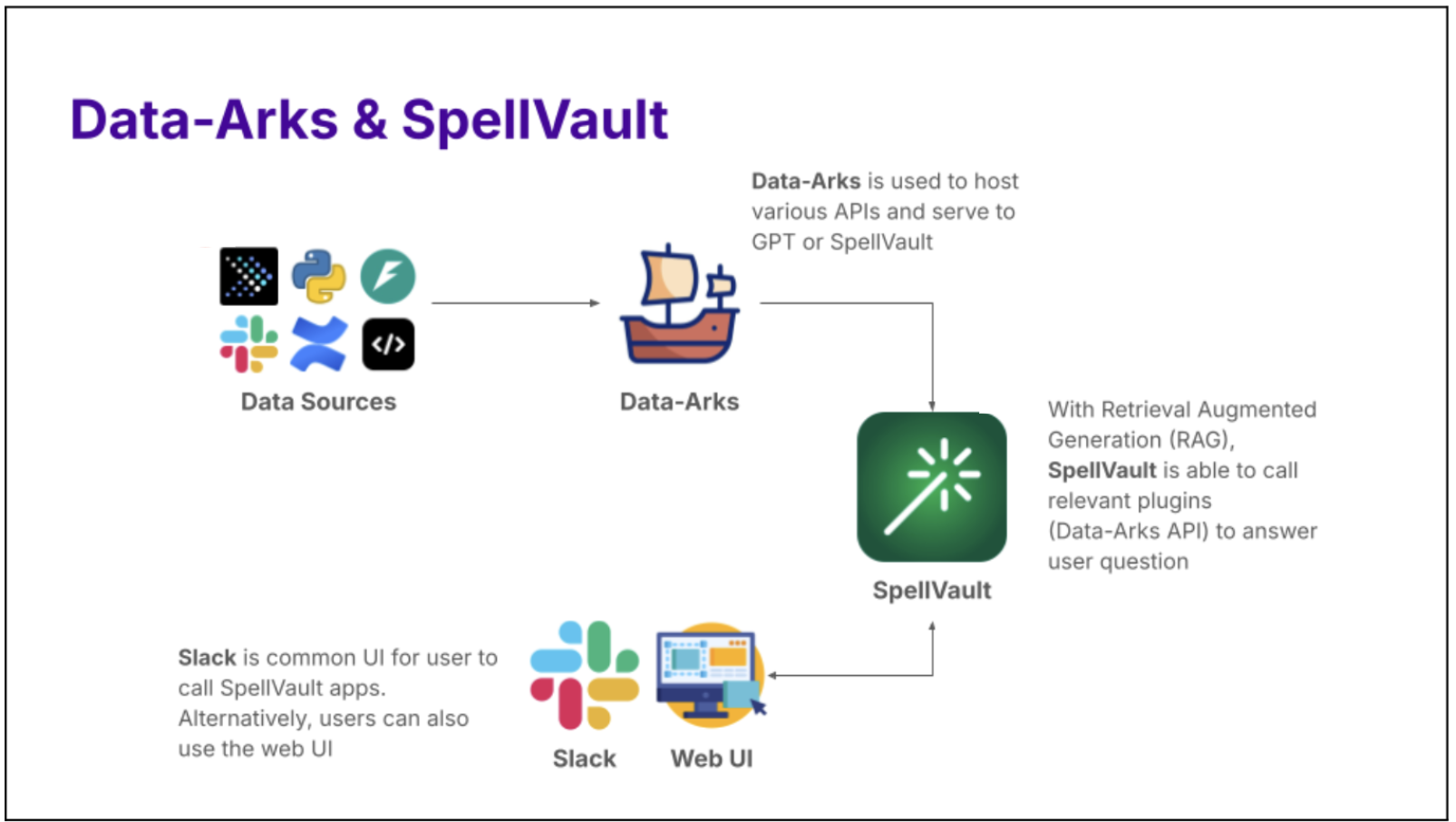
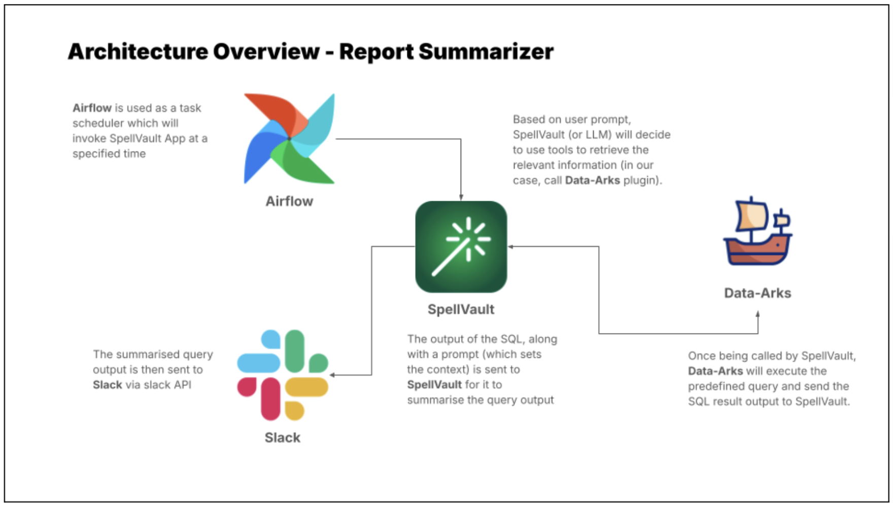
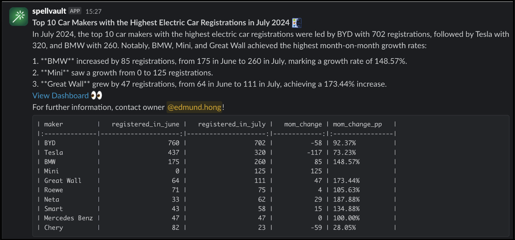
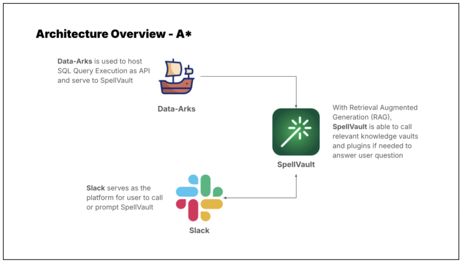
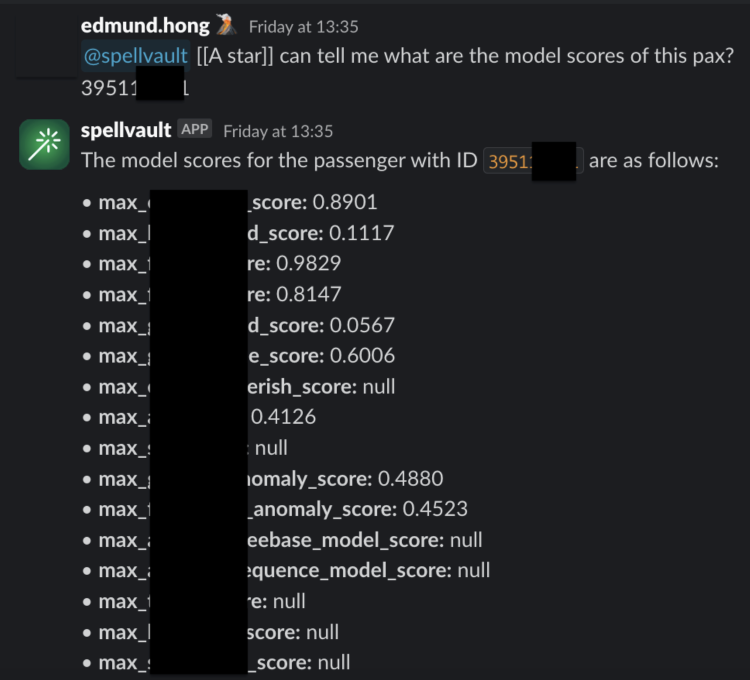
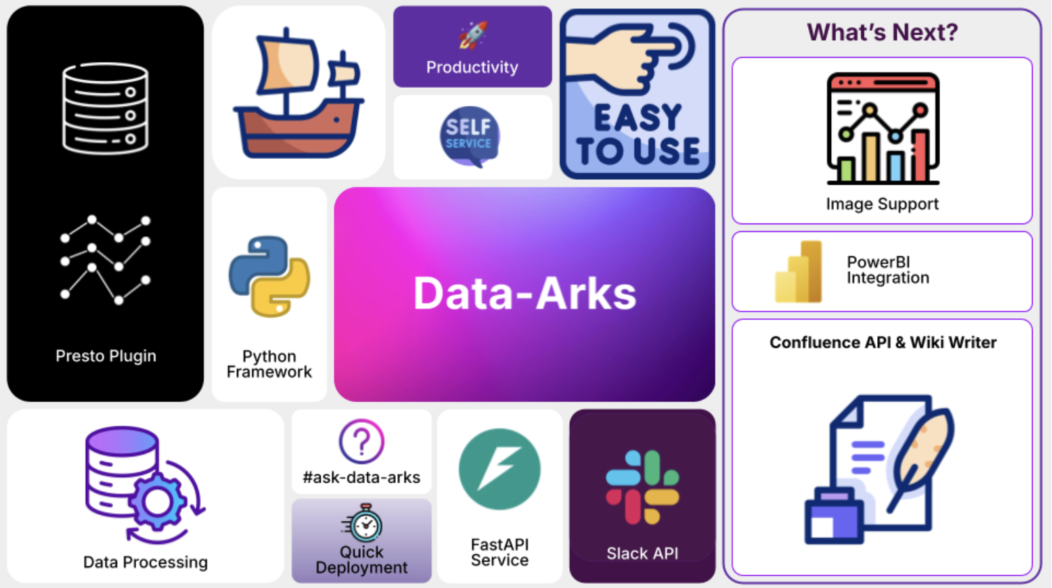


 Erik Iwanski
 Anne Grahn
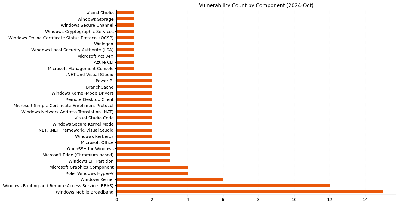
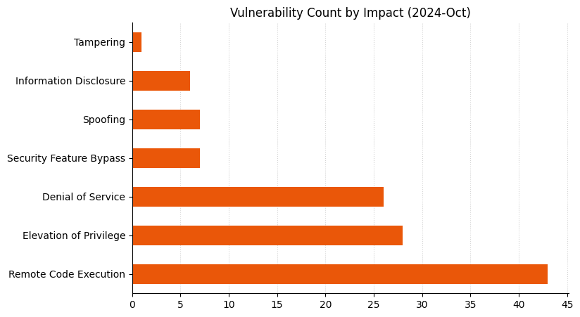
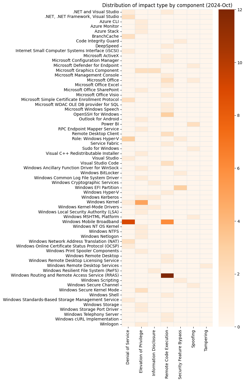

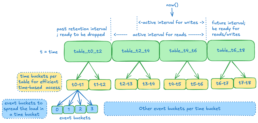
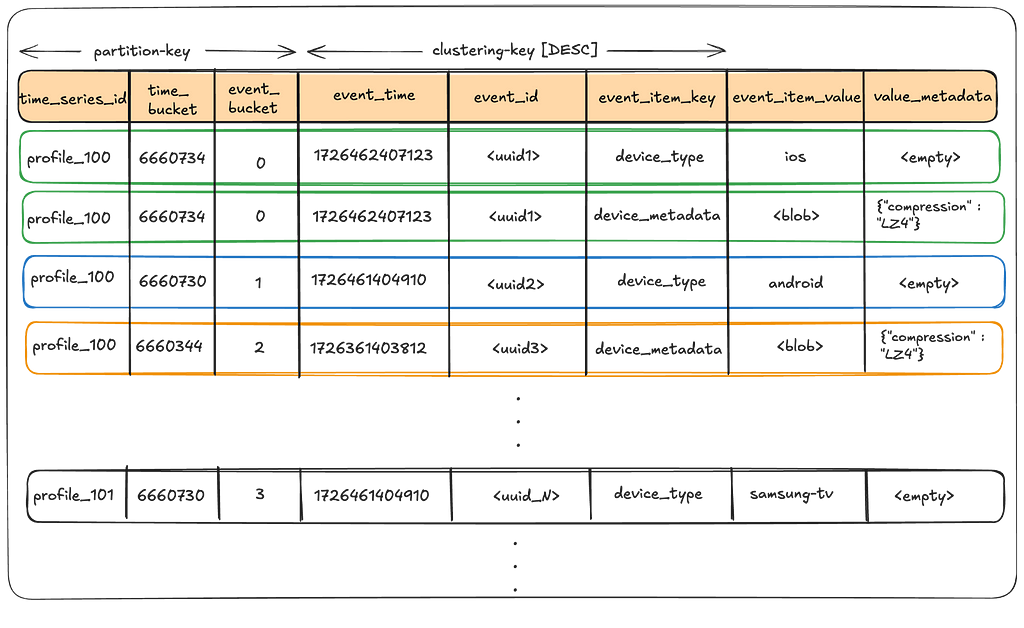

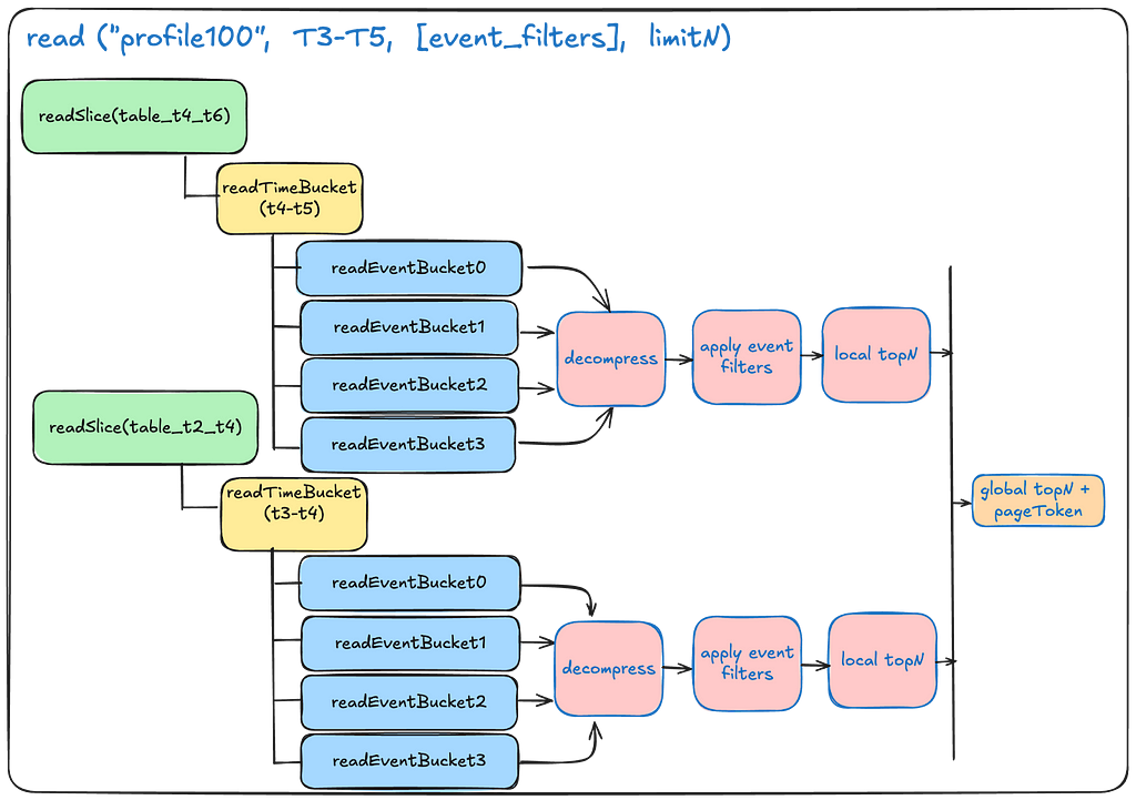
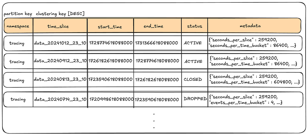
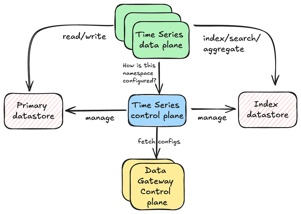
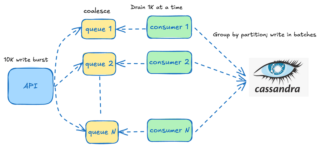
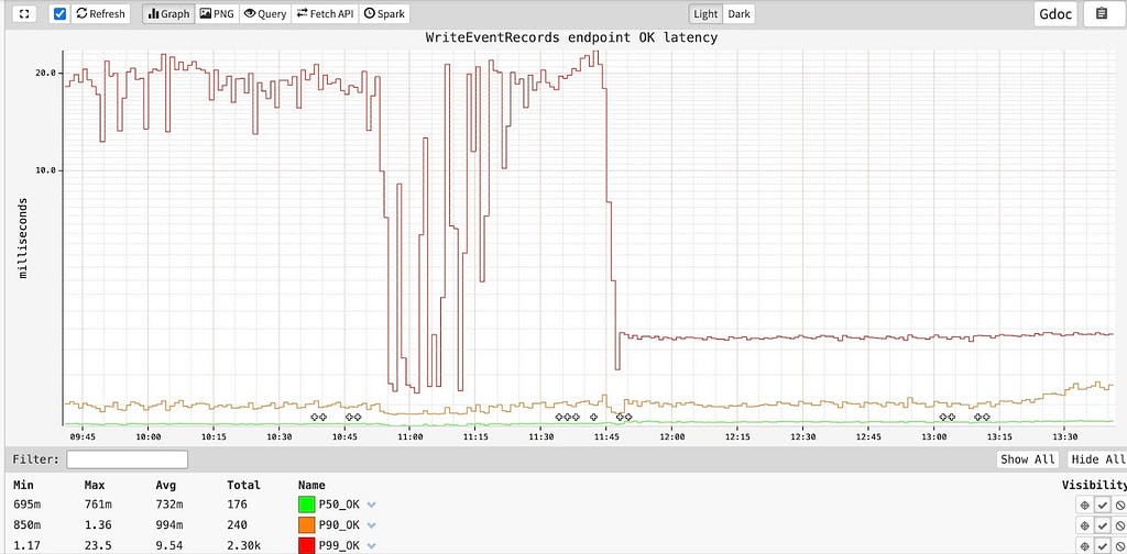
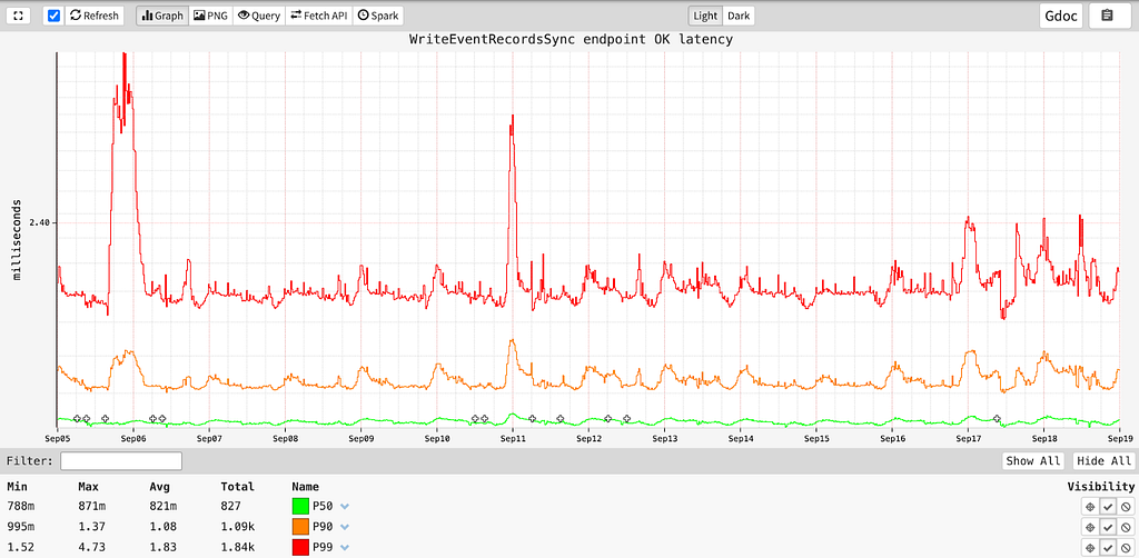
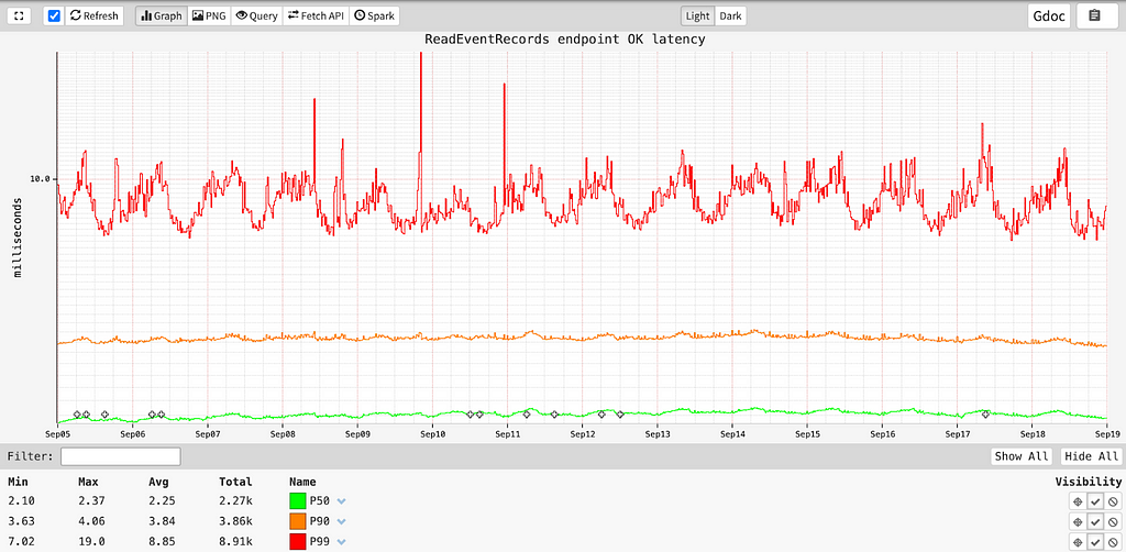
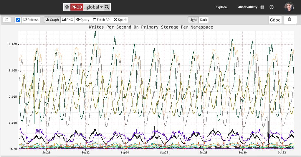
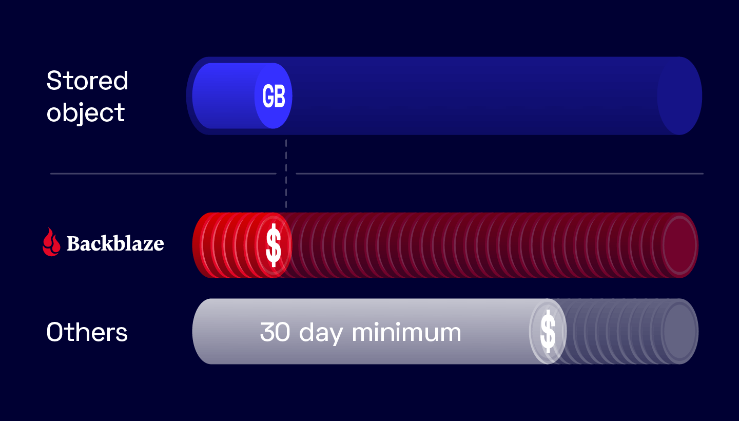


 Tim Wilhoit is a Sr. Solutions Architect for the Department of Defense at AWS. Tim has over 20 years of enterprise IT experience. His areas of interest are serverless computing and ML/AI. In his spare time, Tim enjoys spending time at the lake and rooting on the Oklahoma State Cowboys. Go Pokes!