Залезът на българските божества

Post Syndicated from Емилия Милчева original https://www.toest.bg/zalezut-na-bulgarskite-bozhestva/

Залезът на българските божества

Ако следваме Ницше, чукът ще провери божествата „като камертон“, защото при раняването духът нараства. Раните в политиката не са белезите на воина, там всеки пази не духа, а целофана си. Но ударите могат да бъдат разрушителни не с компромати от телефонни разговори, а с документите и фактите, които може да събере една прокуратура.

Без чадър, без целофан

Тъкмо едно от най-големите политически божества започна да се измества от активната политика към мемориала на знаковите политици – и все-още-главният-прокурор Иван Гешев реши да съживи „Барселонагейт“, като поиска имунитета му. Така изпращането на Бойко Борисов трудно ще бъде съпроводено с почести, още по-малко с добри резултати на местните избори.

Заради собствената си кожа Борисов жертва партията си, спечеленото от нея първо място на 2 април, възможното правителство – и това няма да се размине безнаказано. Принуди ГЕРБ да подкрепи не-коалицията с ПП–ДБ. Дори и да изглежда, че част от парламентарната група му е безрезервно вярна, обкръжението му се готви за ГЕРБ след Борисов – време, което приближава по-бързо, отколкото вероятно му се иска на самия лидер. (През 2019 г. „Тоест“ прогнозира, че третият мандат ще е последен.)

Ако доскоро на гърба на Борисов като същински Атлас тежеше партията, днес е новото мнозинство – ГЕРБ–СДС и ПП–ДБ, което в замяна пази парламента от контакт с Иван Гешев и разказа му за доказателства, свързани с къщата в Барселона и златните кюлчета в нощното шкафче. Няколко тома по делото са в деловодството на Народното събрание и любознателни депутати от разни парламентарни групи четат събрания за близо три години доказателствен материал. От една страна, никой не вярва, че прокуратурата може да събере годни за присъда (за пране на пари) доказателства, от друга – може и да са събирали, но главният прокурор да си е мълчал и трупал за „черни дни“, когато проблемът с неговата безконтролност и безнаказаност ще бъде разрешен законодателно.

Български политически стандарт

Балансът в съюза между ГЕРБ–СДС и ПП–ДБ е крехък – правителството на Денков–Габриел зависи от гласовете на депутатите от ГЕРБ–СДС, за да набере мнозинство. Но ако групата на ПП–ДБ може да взаимодейства само с народните представители на Борисов. За тях обаче полигамията в политическите връзки е практика и я доказват общите гласувания с ДПС, „Възраждане“, „Има такъв народ“ – например по промените в Закона за съдебната власт, които извадиха следствието в отделен от прокуратурата орган. Президентът Румен Радев наложи вето на закона и ще е интересно да се види как и дали и този път ще се образува плаващото мнозинство.

Странно е, че в не-коалицията ГЕРБ–СДС могат да възразят по кадрови решения на министри, като например избора за член на борда на Европейската инвестиционна банка на Виолета Лорер, чиято експертност на финансист е безспорна, но в парламента единодействие по законопроекти до момента няма. С изключение на механизма за разследване на главния прокурор, подкрепен от почти всички политически сили без „Възраждане“, и създаването на комисии – за конституционни промени и за имунитетите.

След възраженията от страна на ГЕРБ–СДС за несъгласуваност министърът на финансите Асен Василев съобщи, че Виолета Лорер, съпруга на политика от ПП Даниел Лорер, се е оттеглила от номинацията и вместо нея ще замине друг експерт с опит от Министерството на финансите – Гергана Беремска. Василев обаче беше категоричен, че реакцията срещу Виолета Лорер е била „непремерена“ и „човек, който е поел тежестта да управлява, трябва да има свободата да управлява“. Партньорът на ПП – „Демократична България“, обаче смята, че механизъм за взаимодействие при ключови назначения трябва да има. Макар да предстоят десетки назначения от парламента в ключови регулатори, такъв механизъм все още не е обсъден нито в коалицията ПП–ДБ, нито в не-коалицията им с ГЕРБ.

Напрежението между двете формации се проявява още в първите дни. В резултат Правната комисия на 49-тото НС отхвърли на първо четене законопроектите за реформа на Антикорупционната комисия (КПКОНПИ), внесени от служебното правителство и от депутати от ПП–ДБ. Подкрепен обаче беше проектозаконът на ГЕРБ–СДС и отново пролича, че политическата сила на Борисов е в състояние да си осигури по-широка от официално договорената подкрепа.

За разлика от избирателите на ПП–ДБ, гласоподавателите на ГЕРБ не са притеснени особено от фигурата на олигарха Делян Пеевски. Знаковото му изтикване на преден план от ДПС като виден конституционалист обаче предизвиква разнопосочни коментари както сред електората на ПП–ДБ, така и в самите партии. А гласуването с „въздържал се“ на лидерите на ПП–ДБ по предложението Пеевски да влезе в Конституционната комисия остави чувството за нещо скрито в тесен формат, още повече след като избегнаха публични обяснения за вота си.

Депутатът от ДПС отдавна е политик без целофан, още от протестите през 2013–2014 г., които го осветиха. Но с приобщаването на ДПС към т.нар. конституционно мнозинство той вече е в друга координатна система и ако ползваме Толкин наратива на силите на Промяната – не е от силите на Мрака.

Кой идва след Иван Гешев?

Временно изпълняващият длъжността главен прокурор, който ще бъде избран на мястото на Иван Гешев, на практика може да изкара много дълго време. Може и да има друга гледна точка за имунитетите на Борисов и други депутати. Например че няма да иска снемането им. Но най-напред президентът трябва да подпише указа за освобождаването на Гешев – ако не реши да оспори мотивите за решението на Висшия съдебен съвет.

От ПП–ДБ изразяват публично мнение, че титулярят на поста трябва да бъде избран, след като се извършат промените, свързани със съдебната реформа. Ако тези заявки бъдат изпълнени, временно изпълняващият длъжността обвинител №1 може да се радва на дълголетието на служебната власт, та дори и повече.

Установено е, че институцията главен прокурор в България генерира в себе си много юридическа и фактическа власт. Толкова много, че тя корумпира и значително изкушава лицето, което заема този пост, да прекрачи извън закона установените граници на своето поведение. Това трябва да се реформира на конституционно ниво и чак след това да бъде избран главен прокурор,

заяви по bTV тази седмица депутатката от ПП–ДБ Надежда Йорданова.

Какви са критериите за главния прокурор по закон?

  • Способност за придържане и налагане на висок етичен стандарт.
  • Висока професионална компетентност – да притежава задълбочени знания в областта на правото, богат практически опит в съответната област на правото, ръководни и административни умения, изявени аналитични способности.
  • Изявена независимост, воля за налагане на законността, решителност при изпълнение на служебните задължения и принос за утвърждаването на правовата държава.
  • Да притежава развити умения за работа в екип, за мотивиране на колегите си, за търсене и носене на отговорност.

Също така кандидатът трябва да има най-малко 12 години стаж – зачита се работа като стажант-юрист в Министерството на правосъдието, също и като разследващ полицай с висше юридическо образование в МВР, Министерството на отбраната или разследващ митнически инспектор в Агенция „Митници“. За стаж се признава и опитът на длъжност, за която се изисква висше юридическо образование в институциите, органите и мисиите на ЕС, ООН, ОССЕ, НАТО, както и в международни правораздавателни органи или международни организации, създадени по силата на международен договор, по който Република България е страна.

Докато политическите сили се разберат има или няма сегашният ВСС моралното право да избира новия главен прокурор, да се избира след или преди приключване на съдебната реформа и т.н., ще управлява именно този бъдещ, временно изпълняващ длъжността обвинител.

Да влезе новият добър „Гешев“. Все едно обаче – най-големият политически играч ще трябва да напусне сцената. Божеството се счупи.

Научни новини: Котешки популации, сънят на гълъбите, иновации в трансплантациите и малко AI

Post Syndicated from Михаил Ангелов original https://www.toest.bg/nauchni-novini-koteshki-populacii-sunyat-na-gulubite/

Контрол на котешките популации

Научни новини: Котешки популации, сънят на гълъбите, иновации в трансплантациите и малко AI

Антимюлеровият хормон (АМХ) е важен компонент в развитието на ембрионите при хората. Отделянето му в мъжките зародиши спира развитието на мюлеровите канали в женската репродуктивна система. При мъжете той се отделя от тестисите и нивата му са високи от раждането до началото на пубертета.

При жените е обратно – преди пубертета нивата на хормона са ниски, след това се повишават и започват да спадат бавно до достигане на менопаузата. Отделянето му става в яйчниците, и по-точно от фоликулите, образуващи яйцеклетките. Именно поради това измерването на количеството му е един от най-добрите начини за определяне на яйчниковия резерв – колкото повече от хормона може да се засече, толкова повече фоликули (и съответно потенциални яйцеклетки) са на разположение.

Един от страничните ефекти на химиотерапията е преждевременното изчерпване на яйчниковия резерв – най-вероятно поради повишеното активиране на фоликулите. В проучване върху мишки от 2017 г. учени са проверили ефекта на АМХ при приложението на няколко вещества, използвани в антитуморната терапия.

Резултатите показват категорично, че при умерено увеличаване на нивата на хормона броят на запазените фоликули е значително по-висок (между 1,2 и 2,9 пъти в зависимост от медикамента) при мишките, получавали АМХ, поради по-бавното им развитие. При още по-високи нива на хормона фоликулите в яйчниците се потискат напълно, което на практика води до стерилност на опитните гризачи.

Това лежи в основата на текуща разработка, която с помощта на методите за генна терапия и използването на вирусни вектори може да намери потенциално приложение за намаляване на популациите на бездомните котки. С помощта на аденовирус, използван за вектор, в мускулната тъкан на животните е вмъкнат модифициран ген за котешкия вариант на АМХ. Методът работи сходно на ваксините за COVID-19, използващи аденовируси за вмъкване на спайкпротеините в човешкото тяло с цел обучаване на имунната система и създаване на имунитет – подход, считан за безопасен и приложим в медицината.

Котките са понесли процедурата без забележими странични ефекти върху здравето им и експресията на АМХ е била увеличена. При два последващи 4-месечни периода на съвместно съжителство с мъжки (8 и 20 месеца след третиране) нито една от тях не е забременяла, за разлика от трите контролни котки, включени в изследването.

Според данните концентрацията на АМХ е намаляла с времето, но това не се е отразило на крайния ефект от третирането. В двете години, в които животните са наблюдавани преди публикуването на статията, не е забелязан негативен ефект върху тях. Дори важни хормони като естрогена не са се повлияли от потискането на развитието на фоликулите.

Най-вероятно стопаните на домашни любимци ще продължат да разчитат на хирургичната намеса, защото, освен преките ефекти, кастрацията има и други ползи. Поради хормоналните промени котките спират да се разгонват с всички свързани с това промени в поведението, като силно мяукане, изнервеност и маркиране. Важни положителни последици са също удължаването на живота и намаляването на риска от развиване на рак на млечните жлези и други заболявания.

За уличните котки стратегията може да се окаже изключително успешна, защото дори ефективността на терапията да намалее с времето, с няколко вълни на третиране популацията им може да се намали значително. Това би имало много положителни ефекти както за самите котки, чийто живот не е лек и обикновено е няколко пъти по-кратък от този на домашните, така и за екосистемите.

Котките са изключително ефективни хищници, които нанасят големи щети върху популациите на птиците и малките бозайници. Това, комбинирано с някои зоонотични заболявания, които те пренасят, прави възможността за бърза и лесна кастрация на голям брой котки изключително интересна както за групите за хуманно отношение към животните, така и за държавните институции, отделящи немалки ресурси за справяне с този проблем.

Какво сънуват гълъбите

Сънят е изключително важен процес, който се среща при повечето животни. При хората се наблюдават два типа сън – REM (с бързо движение на очите) и NREM (без бързо движение на очите). По време на първия мозъчната активност е висока и тогава сънуваме най-ярките си сънища, докато при втория активността е намалена и гръбначномозъчната течност (ликвор) циркулира около мозъка – предполага се, че това помага за прочистването му от вредни протеинови отлагания, някои от които свързани с развитието на заболявания като алцхаймер.

С помощта на инфрачервени камери, които следят зениците на птиците, и функционален ЯМР, проследяващ активността на мозъка, немски екип е установил, че при птиците протичат много сходни процеси. По време на REM съня в мозъка на гълъбите, включени в експеримента, са се активирали участъците, отговорни за обработката на визуална информация, включително тази по време на полет. Наред с тях активност е установена и в зоните, приемащи усещането за допир от тялото и крилете. Същото се е случило и в амигдалата, за която се предполага, че както при хората регулира емоциите.

Всичко това кара учените да изкажат хипотезата, че гълъбите имат визуални сънища, в които летят и изпитват емоции. В нейна подкрепа е и наблюдаваното рязко свиване на зениците им, което е характерно и по време на ухажване или при проява на агресия.

Но повишената мозъчна активност по време на REM съня може да има и някои странични ефекти. Невронната плътност при птиците е по-висока, отколкото при бозайниците, поради което почистването на натрупванията по мозъка трябва да е по-често и ефективно, отколкото при бозайниците. По време на REM съня се увеличава притокът на кръв в мозъка, което води до по-интензивно движение на ликвора около него. Изследователите смятат, че в комбинация с по-кратките и по-чести фази на REM сън това най-вероятно помага за премахването на вредни протеини от мозъчните тъкани.

Сигурно видът и съдържанието на сънищата при птиците ще останат ненапълно установени. Но дори горната хипотеза да не се потвърди, изследването дава много информация за съня при нова група животни и помага да се направят паралели между съня при птиците и хората. Това би могло да въведе гълъбите като моделни системи за изследване на процеси, които поради етични или други съображения не могат да се наблюдават при хората.

Иновации в сърдечната трансплантация

Вземането на органи за трансплантация от трупен донор обикновено се извършва по два начина – след мозъчна смърт на донора или след спиране на кръвообращението му. Първият е по-често срещан, защото въпреки загубата на мозъчна функция физиологичните процеси в тялото се поддържат и органите се запазват жизнени и в естествено състояние до момента на трансплантация. При спиране на кръвообращението настъпват редица усложнения, тъй като органите и тъканите не получават кислород, вследствие на което започват да се увреждат и сравнително бързо стават негодни за трансплантиране.

Поради това броят на такива операции все още е сравнително малък въпреки общия недостиг на донори. С напредването на медицинските технологии броят на органите, които могат да се използват след спиране на кръвообращението, нараства и прогнозата за успешна трансплантация се увеличава, като процедурата вече се прилага за пациенти с нужда от бъбреци и черен дроб. Доскоро това беше изключително трудно при сърцето, поради което се вземаха органи от донори само след мозъчна смърт.

Възможност за увеличаване на броя на потенциалните донори предлага използването на машина, която поддържа циркулацията и електрическите импулси в експлантираното сърце, т.нар. сърце в кутия. Това е сравнително нова технология и все още се прилага в малко клиники – донякъде защото доскоро нямаше данни за състоянието на пациентите, преминали през трансплантация на такива органи.

След публикуването на изследване, включващо 180 души, разделени на две групи (едните, получили орган от донор в мозъчна смърт, a другите – от донор след спиране на кръвообращението му), вече е известно, че почти няма разлика в успеваемостта на процедурата 6 месеца след провеждането ѝ. При първия подход, който се смята за рутинен, процентът живи реципиенти е бил 90, а при втория – 94. Не е имало съществена разлика и в развитието на сериозни странични ефекти 30 дни след трансплантацията и при двата типа процедури. Според авторите на изследването данните са достатъчно убедителни за внедряване на подхода в повече болнични заведения.

Тази техника ще е полезна и при по-често срещани трансплантации след мозъчна смърт. Традиционната практика е след експлантиране на органа той да бъде поставен в лед за транспорт. Това дава на екипа около 4 часа да стигне до реципиента, което ограничава разстоянието за получаване на органа. Ако сърцето е поставено в машината, то може да бъде поддържано по-дълго време и съответно да пътува по-далеч. Наред с това лекарите имат възможност да проверят дали органът функционира нормално, или има увреждания, преди той да бъде имплантиран, което повишава шанса за успешно протичане на процедурата.

Подобрен от AI алгоритъм за сортиране

Сортирането е важен процес в компютърните технологии, който намира най-различни приложения. Затова разработката и оптимизацията на алгоритмите, с които се извършва, е поле на активна изследователска дейност. Една от задачите е сортирането на малки набори, което от своя страна е част от алгоритмите, използващи разделяне на по-големите набори и сортиране „на порции“.

Въпреки че решенията, използвани в момента, са плод на дългогодишен труд, има възможност за подобрение. Нова разработка на подразделението на Google – DeepMind, успешно е оптимизирала алгоритми за сортиране, разработени от хора, като в някои случаи използваният подход е бил „неинтуитивен“ – с други думи, не е нещо, което би дошло на ум на човек.

AlphaDev е изкуствен интелект, базиран на шампиона по играта „го“ на DeepMind – AlphaZero. Използваният подход за обучение е с утвърждаване (reinforcement learning). При него програмата не получава предварителни знания, а с помощта на многократни итерации върху задачата и посочени награди и наказания тя намира най-подходящия начин за постигане на най-висок резултат, подобно на видеоигра. Именно такава дефиниция използват от компанията – игра на асемблер (най-базовия човешко четим език за програмиране). В нея резултатът се определя от времето за изпълнение на алгоритъма за сортиране – колкото по-кратко е то, толкова по-висок е резултатът.

След задаване на правилата AlphaDev започва своеобразна игра, променяйки части от алгоритъма за сортиране. При всяка промяна се отчита времето за изпълнение и дали полученият резултат отговаря на очаквания – ако се подадат числа в случаен ред, те трябва да бъдат подредени след сортирането. Всеки „рунд“ се оценява и сравнява с предишния, което определя дали ще бъде използван за основа на следващия, или ще бъде отхвърлен. В случая откритата оптимизация е възможността за премахване на една стъпка в алгоритъма за сортиране, което ускорява процедурата с до 70% при боравене с 5 елемента и с около 1,7% при над 250 000.

Според авторите подобни алгоритми се изпълняват трилиарди пъти всеки ден, поради което дори и най-малкото забързване ще допринесе за много спестено процесорно време. Разработката на AlphaDev е публикувана в журнала Nature, а оптимизираният алгоритъм вече е прехвърлен в стандартната C++ библиотека за сортиране и всички програмисти имат свободен достъп до него.

Интересен коментар за тази оптимизация дава потребителят Dimitris Papailiopoulos в Twitter. С две запитвания към GPT-4 той постига същия резултат без необходимостта от отнемащото време и ресурси обучение с утвърждаване. Донякъде задачата му е улеснена, защото вече има насока за начина на подобряване на алгоритъма, но все пак е показателно за напредналото ниво на технологията на OpenAI и потенциала, който крие. Възможност за бъдещи подобрения предоставя използването на изкуствен интелект, сходен на AlphaDev – така може да се откриват иновативни подходи, които не биха хрумнали на човек, а след това те да бъдат оптимизирани с помощта на GPT-4 или следващите му версии.

Заглавно изображение: Микроскопска снимка на стъбло на едногодишен бор, напречен разрез, 100х увеличение. Източник: BCC Bioscience Image Library, CC0 / Flickr

Deploying an automated Amazon CloudWatch dashboard for AWS Outposts using AWS CDK

Post Syndicated from Sheila Busser original https://aws.amazon.com/blogs/compute/deploying-an-automated-amazon-cloudwatch-dashboard-for-aws-outposts-using-aws-cdk/

This post is written by Enrico Liguori, Networking Solutions Architect, Hybrid Cloud and Sumeeth Siriyur, Sr. Hybrid Cloud Solutions Architect.

AWS Outposts is a fully managed service that brings the same AWS infrastructure, services, APIs, and tools to virtually any data center, colocation space, manufacturing floor, or on-premises facility where it might be needed. With Outposts, you can run some AWS services on-premises and connect to a broad range of services available in the local AWS Region. Outposts supports workloads requiring low latency, local data processing, data residency, and application migration.

Outposts capacity is driven as per your compute and storage requirements to run workloads. You can monitor Outposts resources using metrics gathered by Amazon CloudWatch. Using these metrics, you can effectively monitor and manage the Outposts resources as they would in the Region, levereging cloud native tools such as CloudWatch dashboards. Check the Monitoring best practices for AWS Outposts blog post to dive deep into the available monitoring options for Outposts.

CloudWatch dashboards are customizable home pages in the CloudWatch console that can be used to monitor resources running on Outposts in a single view. For example, you can monitor in a single pane the number Amazon EC2 instances used per EC2 instance type, the available capacity of Amazon EBS volumes and Amazon S3 buckets, and the operational status of the service link of Outposts.

As a you start deploying additional Outposts resources as a part of their capacity expansion, they must all be integrated and visualized within CloudWatch in an automated way. Traditionally CloudWatch dashboards are built manually and may be time consuming to tune. This post provides also an overview of building CloudWatch dashboards in an automated way using AWS Cloud Development Kit (AWS CDK).

Overview

CloudWatch metrics available to monitor Outposts resources and capacity

CloudWatch metrics for Outposts are available to customers in all public AWS Regions and AWS GovCloud (US) at no additional cost. We can classify the available metrics in two main categories:

To identify the metrics published under the service specific namespaces, we can leverage metadata in the form of tags. A tag is a label that you assign to an AWS resource and consists of a key and an optional value. For the purpose of the monitoring strategy described in this post, we use a tag that contains the OutpostID of the Outpost where the resource is deployed. In this way, we can easily filter the CloudWatch metrics that we would like to show in our dashboard.

To enforce the assignment of tags to our resources we can implement a tagging strategy using AWS tag Policies and Service Control Policies (SCPs).

The following sections describe two different methods to build a CloudWatch dashboard that includes the different types of metrics described so far. In both cases, we see how particularly useful the presence of tags is to identify the service-specific metrics.

Manual approach to building a CloudWatch dashboard for Outposts

This section describes a manual (i.e., non-automated) approach to building a dashboard that could summarize both the capacity utilization metrics and the service specific metrics for your resources running on Outposts.

The benefit of this approach is that we can implement a fully operational dashboard directly from the CloudWatch console. However, it will simultaneously require more effort to properly tune the dashboard to satisfy your monitoring requirements.

You can start creating the dashboard opening the CloudWatch console and following the steps listed in the public documentation.

To display a metric under AWS/Outposts namespace we can choose any of the widgets available. Based on the nature of the data, we can choose different types of Widgets such as Number, Line, Gauge, Explorer, or you can even build your own custom widget.

Together with the Widget type, we must select Outposts namespace in the metric graph dialog box and then navigate to the specific metric of interest.

In case we are creating the dashboard in a different account than the Outposts owner, we must select the right account in the View data drop-down menu to see the Outposts metric in which we are interested.

View data drop-down menu

After selecting one or more metrics we can select Create widget button.

For the service specific metrics, we recommend using the explorer widget. In this way, we can utilize the tagging strategy described earlier to automatically identify the metrics belonging to the resources running on Outposts. Check the documentation page for a step-by-step guide for creating an explorer widget based on tags.

Automated outpost dashboard

After we’ve seen how to build a dashboard manually from the console, in this secton we describe an automated approach to deploy a dashboard for Outposts through AWS CDK.

AWS CDK is an open source software development framework to model and provision your cloud application resources using familiar programming languages, including TypeScript, JavaScript, Python, C#, and Java. For the solution in this post, we use Python.

Architecture overview

The AWS CDK stack described in this post, assumes that the resources running on Outposts (EC2 instances, S3 buckets, Application Load Balancers (ALBs), and RDS instances) are tagged using the tagging strategy described earlier.

Specifying a tag name and a tag value in a configuration file automatically discovers the resources with that tag and adds the related metrics to the CloudWatch dashboard.

Together with the service specific metrics, it creates a series of widgets that we can use to monitor the capacity available and utilized in each Outpost that belongs to the account where the script is running.

The workflow is made of the following phases:

  1. The AWS CDK stack creates an AWS CodeCommit repository and uploads its own code into it. The code contains a series of modules, one for each section of the CloudWatch dashboard. A section of the dashboard contains one or more widgets showing the metrics of a specific service.
  2. To maintain the CloudWatch dashboard always up-to-date with the resources matching the tag, it creates a pipeline in AWS CodePipeline that can dynamically create and or update the dashboard. The pipeline runs the code in the CodeCommit repository and is made of two stages. In the first one, the build stage, it builds the dependencies needed by the AWS CDK stack. In the second stage, the Deploy stage, it loads and runs the modules used to build the dashboard.
  3. Each module contains the code to automatically discover the tagged resources of a specific service. This discovery phase uses standard AWS APIs called through the Python SDK Boto3.
  4. Based on the results of the discovery phase, AWS CDK produces an AWS CloudFormation template containing the definition of the CloudWatch dashboard sections. The template is submitted to CloudFormation.
  5. CloudFormation creates or, if already defined, updates the CloudWatch dashboard.
  6. Together with the dashboard, the AWS CDK script also contains the definition of a CloudWatch Event that, once deployed, triggers the pipeline each time a resource tagged with the specified tag is created or destroyed.

Prerequisites

To implement the solution presented in this post, you must configure:

  1. git as distributed version control system.
  2. In case it is the first time that you’re using AWS CDK in this account and region, you must:

a. Install the AWS CDK, and its prerequisites, following these instructions.

b. Go through the AWS CDK bootstrapping process. This is required only for the first time that we use AWS CDK in a specific AWS environment (an AWS environment is a combination of an AWS account and Region).

How to install

Step 1: Clone the AWS CDK code hosted on GitHub with:

$ git clone https://github.com/aws-samples/automated-cloudwatch-dashboard.git

Step 2: enter the directory using the following:

$ cd  automated-cloudwatch-dashboard/

Step 3: Install the needed Python dependencies with:

$ pip install -r requirements.txt

Step 4: Modify the configuration file

Before deploying the stack, we must modify the configuration file to specify the tag we use for identifying our resources running on Outposts. Open the file with the name config.yaml with your preferred text editor and specify:

      • A name for the dashboard. The default name used is Automated-CloudWatch-Dashboard.
      • Replace <tag_name> placeholder following the tag_name variable with the tag name used to tag the resources that you want to include in the dashboard.
      • Replace <tag_value> placeholder under tag_values variable with the tag value that you used.

Here is an example config.yaml configuration file:

dashboard_name: Automated-CloudWatch-Dahsboard
tag_name: OutpostID
tag_values:
  - op-1234567890abcdefg 

Stack deployment

We can deploy the stack with the following:

$ cdk deploy

At the end of the deployment process, the pipeline that creates the dashboard is provisioned. You can now go to your CloudWatch console to view it.

Automated Outposts dashboard overview

Now that we have built our dashboard, let’s review each section:

  1. Outpost capacity

Outpost Capacity diagram

The AWS CDK stacks define a capacity section for each Outpost available to the AWS account where the script runs.

In this section, we find four widgets showing metrics published under the AWS/Outpost namespace. The first widget shows for each EC2 instance type available on the Outposts the number of instances utilized and available for that instance type. In the second row, we can visualize the available capacity for the Amazon EBS volumes and for the S3 buckets. The last widget shows the operational status of the service link of Outposts.

2. EC2 instances

CPU, Network, and Disk Utilization for an EC2 instance diagram

In this section of the dashboard, we find the metrics showing the CPU, Network, and Disk Utilization for an EC2 instance. It has defined a section of this type for each EC2 instance with a tag assigned matching the name and the value specified in the configuration file of the script.

3. Application Load Balancer

The ALB section aggregates metrics showing the operational status of a load balancer hosted on Outposts

The ALB section aggregates metrics showing the operational status of a load balancer hosted on Outposts. A section of this type is defined for each ALB with an assigned tag matching the one specified in the configuration file.

4. S3 buckets

The S3 buckets section diagram

The S3 buckets section is defined only once and aggregates the utilization metrics for all S3 buckets with an assigned tag.

5. AutoScaling group

The AutoScaling group section diagram

The AutoScaling group section can be used to monitor the number of instances in service in a specific AS group with a tag assigned. This section is defined once and can aggregate the metrics for multiple AutoScaling groups.

Clean up

To terminate the resources that we created in this post, run the following:

$ cdk destroy

Then, go to the Cloudformation console and delete the stack with the name “Deploy-AutomatedCloudWatchDashboard”.

Conclusion

In conclusion, this post demonstrates a manual way of creating CloudWatch Metrics dashboard using the CloudWatch console and an automated way using AWS CDK. The automated approach is also scalable by automatically discovering any new resources added to the existing Outposts in the your environment without any changes to the code.

HPE ProLiant RL300 Gen11 Review A Leadership Ampere Altra Max Arm Server

Post Syndicated from Patrick Kennedy original https://www.servethehome.com/hpe-proliant-rl300-gen11-review-an-ampere-altra-max-arm-server/

The HPE ProLiant RL300 Gen11 is a new leadership cloud-native Ampere Altra Max Arm platform bringing 128 Arm cores to the ProLiant ecosystem

The post HPE ProLiant RL300 Gen11 Review A Leadership Ampere Altra Max Arm Server appeared first on ServeTheHome.

Improved resiliency with backpressure and admission control for Amazon OpenSearch Service

Post Syndicated from Ketan Verma original https://aws.amazon.com/blogs/big-data/improved-resiliency-with-backpressure-and-admission-control-for-amazon-opensearch-service/

Amazon OpenSearch Service is a managed service that makes it simple to secure, deploy, and operate OpenSearch clusters at scale in the AWS Cloud. Last year, we introduced Shard Indexing Backpressure and admission control, which monitors cluster resources and incoming traffic to selectively reject requests that would otherwise pose stability risks like out of memory and impact cluster performance due to memory contentions, CPU saturation and GC overhead, and more.

We are now excited to introduce Search Backpressure and CPU-based admission control for OpenSearch Service, which further enhances the resiliency of clusters. These improvements are available for all OpenSearch versions 1.3 or higher.

Search Backpressure

Backpressure prevents a system from being overwhelmed with work. It does so by controlling the traffic rate or by shedding excessive load in order to prevent crashes and data loss, improve performance, and avoid total failure of the system.

Search Backpressure is a mechanism to identify and cancel in-flight resource-intensive search requests when a node is under duress. It’s effective against search workloads with anomalously high resource usage (such as complex queries, slow queries, many hits, or heavy aggregations), which could otherwise cause node crashes and impact the cluster’s health.

Search Backpressure is built on top of the task resource tracking framework, which provides an easy-to-use API to monitor each task’s resource usage. Search Backpressure uses a background thread that periodically measures the node’s resource usage and assigns a cancellation score to each in-flight search task based on factors like CPU time, heap allocations, and elapsed time. A higher cancellation score corresponds to a more resource-intensive search request. Search requests are cancelled in descending order of their cancellation score to recover nodes quickly, but the number of cancellations is rate-limited to avoid wasteful work.

The following diagram illustrates the Search Backpressure workflow.

Search requests return an HTTP 429 “Too Many Requests” status code upon cancellation. OpenSearch returns partial results if only some shards fail and partial results are allowed. See the following code:

{
    "error": {
        "root_cause": [
            {
                "type": "task_cancelled_exception",
                "reason": "cancelled task with reason: heap usage exceeded [403mb >= 77.6mb], elapsed time exceeded [1.7m >= 45s]"
            }
        ],
        "type": "search_phase_execution_exception",
        "reason": "SearchTask was cancelled",
        "phase": "fetch",
        "grouped": true,
        "failed_shards": [
            {
                "shard": 0,
                "index": "nyc_taxis",
                "node": "9gB3PDp6Speu61KvOheDXA",
                "reason": {
                    "type": "task_cancelled_exception",
                    "reason": "cancelled task with reason: heap usage exceeded [403mb >= 77.6mb], elapsed time exceeded [1.7m >= 45s]"
                }
            }
        ],
        "caused_by": {
            "type": "task_cancelled_exception",
            "reason": "cancelled task with reason: heap usage exceeded [403mb >= 77.6mb], elapsed time exceeded [1.7m >= 45s]"
        }
    },
    "status": 429
}

Monitoring Search Backpressure

You can monitor the detailed Search Backpressure state using the node stats API:

curl -X GET "https://{endpoint}/_nodes/stats/search_backpressure"

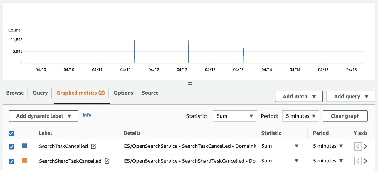
You can also view the cluster-wide summary of cancellations using Amazon CloudWatch. The following metrics are now available in the ES/OpenSearchService namespace:

  • SearchTaskCancelled – The number of coordinator node cancellations
  • SearchShardTaskCancelled – The number of data node cancellations

The following screenshot shows an example of tracking these metrics on the CloudWatch console.

CPU-based admission control

Admission control is a gatekeeping mechanism that proactively limits the number of requests to a node based on its current capacity, both for organic increases and spikes in traffic.

In addition to the JVM memory pressure and request size thresholds, it now also monitors each node’s rolling average CPU usage to reject incoming _search and _bulk requests. It prevents nodes from being overwhelmed with too many requests leading to hot spots, performance problems, request timeouts, and other cascading failures. Excessive requests return an HTTP 429 “Too Many Requests” status code upon rejection.

Handling HTTP 429 errors

You’ll receive HTTP 429 errors if you send excessive traffic to a node. It indicates either insufficient cluster resources, resource-intensive search requests, or an unintended spike in the workload.

Search Backpressure provides the reason for rejection, which can help fine-tune resource-intensive search requests. For traffic spikes, we recommend client-side retries with exponential backoff and jitter.

You can also follow these troubleshooting guides to debug excessive rejections:

Conclusion

Search Backpressure is a reactive mechanism to shed excessive load, while admission control is a proactive mechanism to limit the number of requests to a node beyond its capacity. Both work in tandem to improve the overall resiliency of an OpenSearch cluster.

Search Backpressure is available in OpenSearch, and we are always looking for external contributions. You can refer to the RFC to get started.


About the authors

Ketan Verma is a Senior SDE working on Amazon OpenSearch Service. He is passionate about building large-scale distributed systems, improving performance, and simplifying complex ideas with simple abstractions. Outside work, he likes to read and improve his home barista skills.

Suresh N S is a Senior SDE working on Amazon OpenSearch Service. He is passionate towards solving problems in large scale distributed systems.

Pritkumar Ladani is an SDE-2 working on Amazon OpenSearch Service. He likes to contribute to open source software development, and is passionate about distributed systems. He is an amateur badminton player and enjoys trekking.

Bukhtawar Khan is a Principal Engineer working on Amazon OpenSearch Service. He is interested in building distributed and autonomous systems. He is a maintainer and an active contributor to OpenSearch.

Secure Connectivity from Public to Private: Introducing EC2 Instance Connect Endpoint

Post Syndicated from Sheila Busser original https://aws.amazon.com/blogs/compute/secure-connectivity-from-public-to-private-introducing-ec2-instance-connect-endpoint-june-13-2023/

This blog post is written by Ariana Rahgozar, Solutions Architect, and Kenneth Kitts, Sr. Technical Account Manager, AWS.

Imagine trying to connect to an Amazon Elastic Compute Cloud (Amazon EC2) instance within your Amazon Virtual Private Cloud (Amazon VPC) over the Internet. Typically, you’d first have to connect to a bastion host with a public IP address that your administrator set up over an Internet Gateway (IGW) in your VPC, and then use port forwarding to reach your destination.

Today we launched Amazon EC2 Instance Connect (EIC) Endpoint, a new feature that allows you to connect securely to your instances and other VPC resources from the Internet. With EIC Endpoint, you no longer need an IGW in your VPC, a public IP address on your resource, a bastion host, or any agent to connect to your resources. EIC Endpoint combines identity-based and network-based access controls, providing the isolation, control, and logging needed to meet your organization’s security requirements. As a bonus, your organization administrator is also relieved of the operational overhead of maintaining and patching bastion hosts for connectivity. EIC Endpoint works with the AWS Management Console and AWS Command Line Interface (AWS CLI). Furthermore, it gives you the flexibility to continue using your favorite tools, such as PuTTY and OpenSSH.

In this post, we provide an overview of how the EIC Endpoint works and its security controls, guide you through your first EIC Endpoint creation, and demonstrate how to SSH to an instance from the Internet over the EIC Endpoint.

EIC Endpoint product overview

EIC Endpoint is an identity-aware TCP proxy. It has two modes: first, AWS CLI client is used to create a secure, WebSocket tunnel from your workstation to the endpoint with your AWS Identity and Access Management (IAM) credentials. Once you’ve established a tunnel, you point your preferred client at your loopback address (127.0.0.1 or localhost) and connect as usual. Second, when not using the AWS CLI, the Console gives you secure and seamless access to resources inside your VPC. Authentication and authorization is evaluated before traffic reaches the VPC. The following figure shows an illustration of a user connecting via an EIC Endpoint:

Figure 1 shows a user connecting to private EC2 instances within a VPC through an EIC Endpoint

Figure 1. User connecting to private EC2 instances through an EIC Endpoint

EIC Endpoints provide a high degree of flexibility. First, they don’t require your VPC to have direct Internet connectivity using an IGW or NAT Gateway. Second, no agent is needed on the resource you wish to connect to, allowing for easy remote administration of resources which may not support agents, like third-party appliances. Third, they preserve existing workflows, enabling you to continue using your preferred client software on your local workstation to connect and manage your resources. And finally, IAM and Security Groups can be used to control access, which we discuss in more detail in the next section.

Prior to the launch of EIC Endpoints, AWS offered two key services to help manage access from public address space into a VPC more carefully. First is EC2 Instance Connect, which provides a mechanism that uses IAM credentials to push ephemeral SSH keys to an instance, making long-lived keys unnecessary. However, until now EC2 Instance Connect required a public IP address on your instance when connecting over the Internet. With this launch, you can use EC2 Instance Connect with EIC Endpoints, combining the two capabilities to give you ephemeral-key-based SSH to your instances without exposure to the public Internet. As an alternative to EC2 Instance Connect and EIC Endpoint based connectivity, AWS also offers Systems Manager Session Manager (SSM), which provides agent-based connectivity to instances. SSM uses IAM for authentication and authorization, and is ideal for environments where an agent can be configured to run.

Given that EIC Endpoint enables access to private resources from public IP space, let’s review the security controls and capabilities in more detail before discussing creating your first EIC Endpoint.

Security capabilities and controls

Many AWS customers remotely managing resources inside their VPCs from the Internet still use either public IP addresses on the relevant resources, or at best a bastion host approach combined with long-lived SSH keys. Using public IPs can be locked down somewhat using IGW routes and/or security groups. However, in a dynamic environment those controls can be hard to manage. As a result, careful management of long-lived SSH keys remains the only layer of defense, which isn’t great since we all know that these controls sometimes fail, and so defense-in-depth is important. Although bastion hosts can help, they increase the operational overhead of managing, patching, and maintaining infrastructure significantly.

IAM authorization is required to create the EIC Endpoint and also to establish a connection via the endpoint’s secure tunneling technology. Along with identity-based access controls governing who, how, when, and how long users can connect, more traditional network access controls like security groups can also be used. Security groups associated with your VPC resources can be used to grant/deny access. Whether it’s IAM policies or security groups, the default behavior is to deny traffic unless it is explicitly allowed.

EIC Endpoint meets important security requirements in terms of separation of privileges for the control plane and data plane. An administrator with full EC2 IAM privileges can create and control EIC Endpoints (the control plane). However, they cannot use those endpoints without also having EC2 Instance Connect IAM privileges (the data plane). Conversely, DevOps engineers who may need to use EIC Endpoint to tunnel into VPC resources do not require control-plane privileges to do so. In all cases, IAM principals using an EIC Endpoint must be part of the same AWS account (either directly or by cross-account role assumption). Security administrators and auditors have a centralized view of endpoint activity as all API calls for configuring and connecting via the EIC Endpoint API are recorded in AWS CloudTrail. Records of data-plane connections include the IAM principal making the request, their source IP address, the requested destination IP address, and the destination port. See the following figure for an example CloudTrail entry.

Figure 2 shows a sample cloud trail entry for SSH data-plane connection for an IAMUser. Specific entry:  Figure 2. Partial CloudTrail entry for an SSH data-plane connection

EIC Endpoint supports the optional use of Client IP Preservation (a.k.a Source IP Preservation), which is an important security consideration for certain organizations. For example, suppose the resource you are connecting to has network access controls that are scoped to your specific public IP address, or your instance access logs must contain the client’s “true” IP address. Although you may choose to enable this feature when you create an endpoint, the default setting is off. When off, connections proxied through the endpoint use the endpoint’s private IP address in the network packets’ source IP field. This default behavior allows connections proxied through the endpoint to reach as far as your route tables permit. Remember, no matter how you configure this setting, CloudTrail records the client’s true IP address.

EIC Endpoints strengthen security by combining identity-based authentication and authorization with traditional network-perimeter controls and provides for fine-grained access control, logging, monitoring, and more defense in depth. Moreover, it does all this without requiring Internet-enabling infrastructure in your VPC, minimizing the possibility of unintended access to private VPC resources.

Getting started

Creating your EIC Endpoint

Only one endpoint is required per VPC. To create or modify an endpoint and connect to a resource, a user must have the required IAM permissions, and any security groups associated with your VPC resources must have a rule to allow connectivity. Refer to the following resources for more details on configuring security groups and sample IAM permissions.

The AWS CLI or Console can be used to create an EIC Endpoint, and we demonstrate the AWS CLI in the following. To create an EIC Endpoint using the Console, refer to the documentation.

Creating an EIC Endpoint with the AWS CLI

To create an EIC Endpoint with the AWS CLI, run the following command, replacing [SUBNET] with your subnet ID and [SG-ID] with your security group ID:

aws ec2 create-instance-connect-endpoint \
    --subnet-id [SUBNET] \
    --security-group-id [SG-ID]

After creating an EIC Endpoint using the AWS CLI or Console, and granting the user IAM permission to create a tunnel, a connection can be established. Now we discuss how to connect to Linux instances using SSH. However, note that you can also use the OpenTunnel API to connect to instances via RDP.

Connecting to your Linux Instance using SSH

With your EIC Endpoint set up in your VPC subnet, you can connect using SSH. Traditionally, access to an EC2 instance using SSH was controlled by key pairs and network access controls. With EIC Endpoint, an additional layer of control is enabled through IAM policy, leading to an enhanced security posture for remote access. We describe two methods to connect via SSH in the following.

One-click command

To further reduce the operational burden of creating and rotating SSH keys, you can use the new ec2-instance-connect ssh command from the AWS CLI. With this new command, we generate ephemeral keys for you to connect to your instance. Note that this command requires use of the OpenSSH client. To use this command and connect, you need IAM permissions as detailed here.

Once configured, you can connect using the new AWS CLI command, shown in the following figure:
Figure 3 shows the AWS CLI view if successfully connecting to your instance using the one-click command. When running the command, you are prompted to connect and can access your instance.

Figure 3. AWS CLI view upon successful SSH connection to your instance

To test connecting to your instance from the AWS CLI, you can run the following command where [INSTANCE] is the instance ID of your EC2 instance:

aws ec2-instance-connect ssh --instance-id [INSTANCE]

Note that you can still use long-lived SSH credentials to connect if you must maintain existing workflows, which we will show in the following. However, note that dynamic, frequently rotated credentials are generally safer.

Open-tunnel command

You can also connect using SSH with standard tooling or using the proxy command. To establish a private tunnel (TCP proxy) to the instance, you must run one AWS CLI command, which you can see in the following figure:

Figure 4 shows the AWS CLI view after running the aws ec2-instance-connect open-tunnel command and connecting to your instance.Figure 4. AWS CLI view after running new SSH open-tunnel command, creating a private tunnel to connect to our EC2 instance

You can run the following command to test connectivity, where [INSTANCE] is the instance ID of your EC2 instance and [SSH-KEY] is the location and name of your SSH key. For guidance on the use of SSH keys, refer to our documentation on Amazon EC2 key pairs and Linux instances.

ssh ec2-user@[INSTANCE] \
    -i [SSH-KEY] \
    -o ProxyCommand='aws ec2-instance-connect open-tunnel \
    --instance-id %h'

Once we have our EIC Endpoint configured, we can SSH into our EC2 instances without a public IP or IGW using the AWS CLI.

Conclusion

EIC Endpoint provides a secure solution to connect to your instances via SSH or RDP in private subnets without IGWs, public IPs, agents, and bastion hosts. By configuring an EIC Endpoint for your VPC, you can securely connect using your existing client tools or the Console/AWS CLI. To learn more, visit the EIC Endpoint documentation.

CVE-2023-34362: MOVEit Vulnerability Timeline of Events

Post Syndicated from Rapid7 original https://blog.rapid7.com/2023/06/14/etr-cve-2023-34362-moveit-vulnerability-timeline-of-events/

CVE-2023-34362: MOVEit Vulnerability Timeline of Events

The following article was written by Drew Burton and Cynthia Wyre.

Rapid7 continues to track the impact of CVE-2023-34362, a critical zero-day vulnerability in Progress Software’s MOVEit Transfer solution. CVE-2023-34362 allows for SQL injection, which can result in unauthorized access to sensitive data, such as passwords, credit card details, or personal user information.

Rapid7 is not currently seeing evidence that commodity or low-skill attackers are exploiting the vulnerability. However, the exploitation of available high-value targets globally across a wide range of org sizes, verticals, and geo-locations indicates that this is a widespread threat. We expect to see a longer list of victims come out as time goes on.

We’ve put together a timeline of events to date for your reference.

MOVEit Timeline

May 27-28: Rapid7 services teams have so far confirmed indicators of compromise and data exfiltration dating back to at least May 27 and May 28, 2023 (respectively).

May 31: Progress Software publishes an advisory on a critical SQL injection vulnerability in their MOVEit Transfer solution.

May 31: Rapid7 begins investigating exploitation of MOVEit Transfer.

June 1: Rapid7 publishes initial analysis of MOVEit Transfer attacks after responding to incidents across multiple customer environments.

June 1: The security community publishes technical details and indicators of compromise.

June 1: Compromises continue; Rapid7 responds to alerts.

June 1: CISA publishes Security Advisory.

June 2: CVE-2023-34362 is assigned to the zero-day vulnerability.

June 2: Mandiant attributes the attack to a threat cluster with unknown motives.

June 2: Velociraptor releases an artifact to detect exploitation of MOVEit File Transfer critical vulnerability.

June 4: Rapid7 publishes a method to identify which data was stolen.

June 4: Nova Scotian government discloses it is investigating privacy breach.

June 5: Microsoft attributes the attack to Lace Tempest, a Cl0p ransomware affiliate that has previously exploited vulnerabilities in other file transfer solutions (e.g., Accellion FTA, Fortra GoAnywhere MFT).

June 5: UK companies BA, BBC, and Boots disclose breaches as victims in MOVEit File Transfer.

June 5: Cl0p ransomware group claims responsibility for the zero-day attack.

June 6: Security firm Huntress releases a video allegedly reproducing the exploit chain.

June 6: The Cl0p ransomware group posts a communication on their leak site demanding that victim organizations contact them by June 14 to negotiate extortion fees in exchange for the deletion of stolen data.

June 7: CISA publishes #StopRansomware Cybersecurity Advisory regarding MOVEit File Transfer Vulnerability CVE-2023-34362.

June 9: Progress Software updates advisory to include a patch for a second MOVEit Transfer Vulnerability, which was uncovered by Huntress during a third-party code review. The vulnerability is later assigned CVE-2023-35036.

June 12: Rapid7 releases a full exploit chain for MOVEit Transfer Vulnerability CVE-2023-34362.

Mitigation

All MOVEit Transfer versions before May 31, 2023 are vulnerable to CVE-2023-34362, and all MOVEit Transfer versions before June 9, 2023 are vulnerable to CVE-2023-35036. As noted above, fixed versions of the software are available, and patches should be applied on an emergency basis.

Patches are available via Progress Software’s CVE-2023-34362 advisory. Additionally, because CVE-2023-34362 is a zero-day vulnerability, Progress Software is advising MOVEit Transfer and MOVEit Cloud customers to check for indicators of unauthorized access over “at least the past 30 days.”

According to the company’s status page, Progress also took the following steps aimed at increasing security monitoring and defending against further exploitation or attack:

  • Developed specific monitoring signatures on Progress’ endpoint protection system.
  • Validated that the newly developed patch corrected the vulnerability.
  • Tested detection rules before finalizing to ensure that notifications are working properly.
  • Engaged outside cybersecurity experts and other incident response professionals to conduct a forensic investigation and assess the extent and scope of the incident.

As noted in the timeline above, Rapid7 has added capabilities across our portfolio that can help users identify and resolve risk from CVE-2023-34362. We have also identified a method to identify exfiltrated data from compromised MOVEit customer environments.

To learn more, check out: Rapid7 Observed Exploitation of Critical MOVEit Transfer Vulnerability

GitHub Availability Report: May 2023

Post Syndicated from Jakub Oleksy original https://github.blog/2023-06-14-github-availability-report-may-2023/

In May, we experienced four incidents that resulted in degraded performance across GitHub services. This report also sheds light into three April incidents that resulted in degraded performance across GitHub services.

April 26 23:11 UTC (lasting 51 minutes)

On April 25 at 23:11 UTC, a subset of users began to see a degraded experience with GitHub Copilot code completions. We publicly statused GitHub Copilot to yellow at 23:26 UTC, and to red at 23:41 UTC. As engineers identified the impact to be a subset of requests, we statused back to yellow at 23:48 UTC. The incident was fully resolved on April 26 at 00:02 UTC, and we publicly statused green at 00:30 UTC.

The degradation consisted of a rolling partial outage across all three GitHub Copilot regions: US Central, US East, and Switzerland North. Each of these regions experienced approximately 15-20 minutes of degraded service during the global incident. At the peak, 6% of GitHub Copilot code completion requests failed.

We identified the root cause to be a faulty configuration change by an automated maintenance process. The process was initiated across all regions sequentially, and placed a subset of faulty nodes in service before the rollout was halted by operators. Automated traffic rollover from the failed nodes and regions helped to mitigate the issue.

Our efforts to prevent a similar incident in the future include both reducing the batch size and iteration speed of the automated maintenance process, and lowering our time to detection by adjusting our alerting thresholds.

April 27 08:59 UTC (lasting 57 minutes)

On April 26 at 08:59 UTC, our internal monitors notified us of degraded availability with GitHub Packages. Users would have noticed slow or failed GitHub Packages upload and download requests. Our investigation revealed a spike in connection errors to our primary database node. We quickly took action to resolve the issue by manually restarting the database. At 09:56 UTC, all errors were cleared and users experienced a complete recovery of the GitHub Packages service. A planned migration of GitHub Packages database to a more robust platform was completed on May 2, 2023 to prevent this issue from recurring.

April 28 12:26 UTC (lasting 19 minutes)

On April 28 at 12:26 UTC, we were notified of degraded availability for GitHub Codespaces. Users in the East US region experienced failures when creating and resuming codespaces. At 12:45 UTC, we used regional failover to redirect East US codespace creates and resumes to the nearest healthy region, East US 2, and users experienced a complete and nearly immediate recovery of GitHub Codespaces.

Our investigation indicated our cloud provider had experienced an outage in the East US region, with virtual machines in that region experiencing internal operation errors. Virtual machines in the East US 2 region (and all other regions) were healthy, which enabled us to use regional failover to successfully recover GitHub Codespaces for our East US users. When our cloud provider’s outage was resolved, we were able to seamlessly direct all of our East US GitHub Codespaces uses back with no downtime.

Long-term mitigation is focused on reducing our time to detection for outages such as this by improving our monitors and alerts, as well as reducing our time to mitigate by making our regional failover tooling and documentation more accessible.

May 4th 15:53 UTC (lasting 30 minutes)

On May 4th at 15:23 UTC, our monitors detected degraded performance for Git Operations, GitHub APIs, GitHub Issues, GitHub Pull Requests, GitHub Webhooks, GitHub Actions, GitHub Pages, GitHub Codespaces, and GitHub Copilot. After troubleshooting we were able to mitigate the issue by performing a primary failover on our repositories database cluster. Further investigation indicated the root cause was connection pool exhaustion on our proxy layer. Prior updates to this configuration were inconsistently applied. We audited and fixed our proxy layer connection pool configurations during this incident, and updated our configuration automation to dynamically apply config changes without disruption to ensure consistent configuration of database proxies moving forward.

May 09 11:27 UTC (lasting 10 hours and 44 minutes)

On May 9 at 11:27 UTC, users began to see failures to read or write Git data. These failures continued until 12:33 UTC, affecting Git Operations, GitHub Issues, GitHub Actions, GitHub Codespaces, GitHub Pull Requests, GitHub Web Hooks, and GitHub APIs. Repositories and GitHub Pull Requests required additional time to fully recover job results and search capabilities, with recovery completing at 21:20 UTC. On May 11 at 13:33 UTC, similar failures occurred affecting the same services until 14:40 UTC. Again, GitHub Pull Requests required additional time to fully recover search capabilities, with recovery completing at 18:54 UTC. We discussed both of these events in a previous blog post and can confirm they share the same root cause.

Based on our investigation we determined that the cause of this crash is due to a bug in the database version we are running, and the conditions causing this bug were more likely to happen in a custom configuration on this data cluster. We updated our configuration to match the rest of our database clusters, and this cluster is no longer vulnerable to this kind of failover.

The bug has since been reported to the database maintainers, accepted as a private bug, and fixed. The fix is slated for a release expected in July.

There have been several directions of work in response to these incidents to avoid reoccurrence. We have focused on removing special case configurations of our database clusters to avoid unpredictable behavior from custom configurations. Across feature areas, we have also expanded tooling around graceful degradation of web pages when dependencies are unavailable.

May 10 12:38 UTC (lasting 11 hours and 56 minutes)

On May 10 at 12:38 UTC, issuance of auth tokens for GitHub Apps started failing, impacting GitHub Actions, GitHub API Requests, GitHub Codespaces, Git Operations, GitHub Pages, and GitHub Pull Requests. We identified the cause of these failures to be a significant increase in write latency on a shared permissions database cluster. First responders mitigated the incident by identifying the data shape in new API calls that was causing very expensive database write transactions and timeouts in a loop and blocking the source. We shared additional details on this incident in a previous blog post, but we wanted to share an update on our follow-up actions. Beyond the immediate work to address the expensive query pattern that caused this incident, we completed an audit of other endpoints to identify and correct any similar patterns. We completed improvements to the observability of API errors and have further work in progress to improve diagnosis of unhealthy MySQL write patterns. We also completed improvements to tools, documentation and playbooks, and training for both the technical diagnosis and our general incident response to address issues encountered while mitigating this issue and to reduce the time to mitigate similar incidents in the future.

May 16 21:07 UTC (lasting 25 minutes)

On May 16 at 21:08 UTC, we were alerted to degradation of multiple services. GitHub Issues, GitHub Pull Requests, and Git Ops were unavailable while GitHub API, GitHub Actions, GitHub Pages, and GitHub Codespaces were all partially unavailable. Alerts indicated that the primary database of a cluster supporting key-value data had experienced a hardware crash. The cluster was left in such a state that our failover automation was unable to select a new primary to promote due to the risk of data loss. Our first responder evaluated the cluster, determined it was safe to proceed, and then manually triggered a failover to a new primary host 11 minutes after the server crash. We aspire to reduce our response time moving forward and are looking into improving our alerting for cases like this. Long-term mitigation is focused on reducing dependency on this cluster as a single point of failure for much of the site.


Please follow our status page for real-time updates on status changes. To learn more about what we’re working on, check out the GitHub Engineering Blog.

Discover How AWS Designed Silicon Fuels Customer Outcomes at AWS Silicon Innovation Day

Post Syndicated from Irshad Buchh original https://aws.amazon.com/blogs/aws/discover-how-aws-designed-silicon-fuels-customer-outcomes-at-aws-silicon-innovation-day/

We hope you will join us on Wednesday, June 21, for a free-to-attend online event, AWS Silicon Innovation Day. AWS will stream the event simultaneously across multiple platforms, including LinkedIn Live, Twitter, YouTube, and Twitch.

AWS Silicon Innovation Day is a one-day virtual event on June 21, 2023, that will allow you to better understand AWS Silicon and how you can use AWS’s unique Amazon EC2 chip offerings to your benefit. AWS has designed and developed purpose-built silicon specifically for the cloud.

During this event, you will have the opportunity to hear directly from senior leaders at AWS. Our panel of lead architects, engineers, customers, and analysts will provide insights into our silicon journey. Through deep dives into our cutting-edge silicon design and customer success stories, the panel will provide insights on security enhancements and cost-saving opportunities. Here are some of the highlights you can expect from this event.

Leadership session – To kick off the day, we have a Leadership session featuring Dave Brown, VP of Amazon EC2 and Dr. Ruba Borno, VP of WW Channels and Alliances joining us on stage. Dave will engage in a discussion with Ruba about how you can benefit from the innovation AWS delivers with its silicon technology.

AI/ML session – Gary Szilagyi, VP of Annapurna Labs will discuss with Nafea Bshara, co-founder of Annapurna Labs the utilization of chipset development by his team to create specialized chips for Generative AI, CPU, and the AWS Nitro system. He will highlight how you can harness the Annapurna mindset to develop not only CPUs but also tailor-made chips with specific purposes in mind.

Customer session – Jeff Barr, VP of AWS Evangelism, and Tiffany Wissner, Director of Product Marketing, will delve into insights from our customers. They will share anecdotes and experiences gathered from various sources, such as re:Invent, summits, and developer events, where you have expressed how you harnessed AWS silicon to drive your own remarkable innovations.

Networking session – JR Rivers, Senior Principal Engineer, and Madhura Kale, Senior Product Manager will shed light on the impact of silicon innovation, not only on the benefits you experience using our CPUs, GPUs, or Nitro System, but also on the transformation of AWS’s network infrastructure. They will delve into the realm of networking advancements, showcasing some of the latest innovations and highlighting the instrumental role played by AWS silicon in powering these developments.

Arm and Nitro Innovation session – Anthony Liguori, VP and Fellow, Nitro System architecture will be joined by Ali Saidi, Director of Annapurna Labs to discuss harnessing the power of hardware and software in tandem to drive the development of cutting-edge silicon technologies.

Analyst and Executive session – Raj Pai, VP of Amazon EC2 Product Management will engage in a conversation with an analyst, delving into the realm of silicon innovation in the cloud.

Join us for Silicon Innovation Day Wednesday June 21 9:00am - 4:00pm PDT

No advance registration is needed to participate in AWS Silicon Innovation Day, but you can add an event reminder to your calendar by registering on the event page. We sincerely hope that you will join us in embracing the excitement and seizing the valuable learning opportunities at this new event!

Meet you there.

— Irshad

Removing header remapping from Amazon API Gateway, and notes about our work with security researchers

Post Syndicated from Mark Ryland original https://aws.amazon.com/blogs/security/removing-header-remapping-from-amazon-api-gateway-and-notes-about-our-work-with-security-researchers/

At Amazon Web Services (AWS), our APIs and service functionality are a promise to our customers, so we very rarely make breaking changes or remove functionality from production services. Customers use the AWS Cloud to build solutions for their customers, and when disruptive changes are made or functionality is removed, the downstream impacts can be significant. As builders, we’ve felt the impact of these types of changes ourselves, and we work hard to avoid these situations whenever possible.

When we do need to make breaking changes, we try to provide a smooth path forward for customers who were using the old functionality. Often that means changing the behavior for new users or new deployments, and then allowing a transition window for existing customers to migrate from the old to the new behavior. There are many examples of this pattern, such as an update to IAM role trust policy behavior that we made last year.

This post explains one such recent change that we’ve made in Amazon API Gateway. We also discuss how we work with the security research community to improve things for customers.

Summary and customer impact

Recently, researchers at Omegapoint disclosed an edge case issue with how API Gateway handled HTTP header remapping with custom authorizers based on AWS Lambda. As is often the case with security research, this work generated a second, tangentially related authorization-caching issue that the Omegapoint team also reported.

After analyzing these reports, the API Gateway team decided to remove a documented feature from the service and to adjust another behavior to improve service behavior. We’ve made the appropriate changes to the API Gateway documentation.

As of June 14, 2023, the header remapping feature is no longer available in API Gateway. Customers can still use Velocity Template Language-based (VTL) transformations for header remapping, because this approach wasn’t impacted by the reported issue. If you’re using this design pattern in API Gateway and have questions about this change, reach out to your AWS support team.

The authorization-caching behavior was working as originally designed; but based on the report, we’ve adjusted it to better meet customer expectations.

The team at Omegapoint has published their findings in the blog post Writeup: AWS API Gateway header smuggling and cache confusion.

Before we removed the feature, we contacted customers who were using the direct HTTP header remapping feature through email and the AWS Health Dashboard. If you haven’t been contacted, no action is required on your part.

More details

The main issue that Omegapoint reported was related to a documented, client-controlled HTTP header remapping feature in API Gateway. This feature allowed customers to use one set of header values in the interaction between their clients and API Gateway, and a different set of header values from API Gateway to the backend. The client could send two sets of header values: one for API Gateway and one for the backend. API Gateway would process both sets, but then remap (overwrite) one set of values with another set. This feature was especially useful when allowing newly created API Gateway clients to continue to work with legacy servers whose header-handling logic couldn’t be modified.

The report from Omegapoint highlighted that customers who relied on Lambda authorizers for request-based authorization could be surprised when the remapping feature was used to overwrite header values that were used for further authorization on the backend, which could potentially lead to unintended access. The Lambda authorizer itself worked as expected on unmapped headers, but if there was additional authorization logic in the backend, it could be impacted by a misbehaving client.

The second issue that Omegapoint reported was related to the caching behavior in API Gateway for authorization policies. Previously, the caching method might reuse a cached authorization with a different value when the <method.request.multivalueheader.*> value was used in the request header within the time-to-live (TTL) of the cached value. This was the expected behavior of the wildcard value.

However, after reviewing the report, we agreed that it could surprise customers, and potentially allow misbehaving clients to bypass expected authorization. We were able to change this behavior without customer impact, because there is no evidence of customers relying on this behavior. So now, cached authorizations are no longer used in the <multivalueheader> case.

How we work with researchers

Security researchers regularly submit vulnerability reports to AWS Security. Some researchers are independent, some work in academic institutions, and others work in AWS partner or customer organizations. Our Outreach team triages submissions rapidly. Upon receipt, we start a conversation and work closely with researchers to understand their concerns, give our perspective, and agree on the best path forward.

If technical changes are required, our services and security teams work together to determine and implement the appropriate remediations based on the potential impact. They work with affected customers to reduce or eliminate impacts, and they work with the researchers to coordinate the publication of their findings.

Often these reports highlight situations where the designed and documented behavior might result in a surprising outcome for some customers. In those cases, we work with the researcher to make the appropriate updates to the documentation, if needed, and help ensure that the researcher’s finding is published with customer education as the primary goal.

In other cases, where warranted, we communicate about security issues to the broader customer and security community by using a security bulletin. Finally, we publish security blog posts in cases where providing more context makes sense, such as the current issue.

Security is our top priority, and working with the community to make our customers and the AWS Cloud safer is a key part of that. Clear communication helps build understanding and trust.

Working together

We removed the direct remapping feature because not many customers were using it, and we felt that documentation warning against the impacted design choices provided insufficient visibility and protection for customers. We designed and released the feature in an era when it was reasonable to assume that an API Gateway client would be well-behaved, but as times change, it now makes sense that an API client could be potentially negligent or even hostile. There are multiple alternative approaches that can provide the same outcome for customers, but in a more expected and controlled manner, which made this a simpler process to work through.

When researchers report potential security findings, we work through our process to determine the best outcome for our customers. In most cases, we can adjust designs to address the issue, while maintaining the affected features.

In rare cases, such as this one, the more effective path forward is to sunset a feature in favor of a more expected and secure approach. This is a core principle of evolving architectures and building resilient systems. It’s something that we practice regularly at AWS and a key principle that we share with our customers and the community through the AWS Well-Architected Framework.

Our thanks to the team at Omegapoint for reporting these issues, and to all of the researchers who continue to work with us to help make the AWS Cloud safer for our customers.

Want more AWS Security news? Follow us on Twitter.

Mark Ryland

Mark Ryland

Mark is the director of the Office of the CISO for AWS. He has over 30 years of experience in the technology industry, and has served in leadership roles in cybersecurity, software engineering, distributed systems, technology standardization, and public policy. Previously, he served as the Director of Solution Architecture and Professional Services for the AWS World Public Sector team.

Migrating Netflix to GraphQL Safely

Post Syndicated from Netflix Technology Blog original https://netflixtechblog.com/migrating-netflix-to-graphql-safely-8e1e4d4f1e72

By Jennifer Shin, Tejas Shikhare, Will Emmanuel

In 2022, a major change was made to Netflix’s iOS and Android applications. We migrated Netflix’s mobile apps to GraphQL with zero downtime, which involved a total overhaul from the client to the API layer.

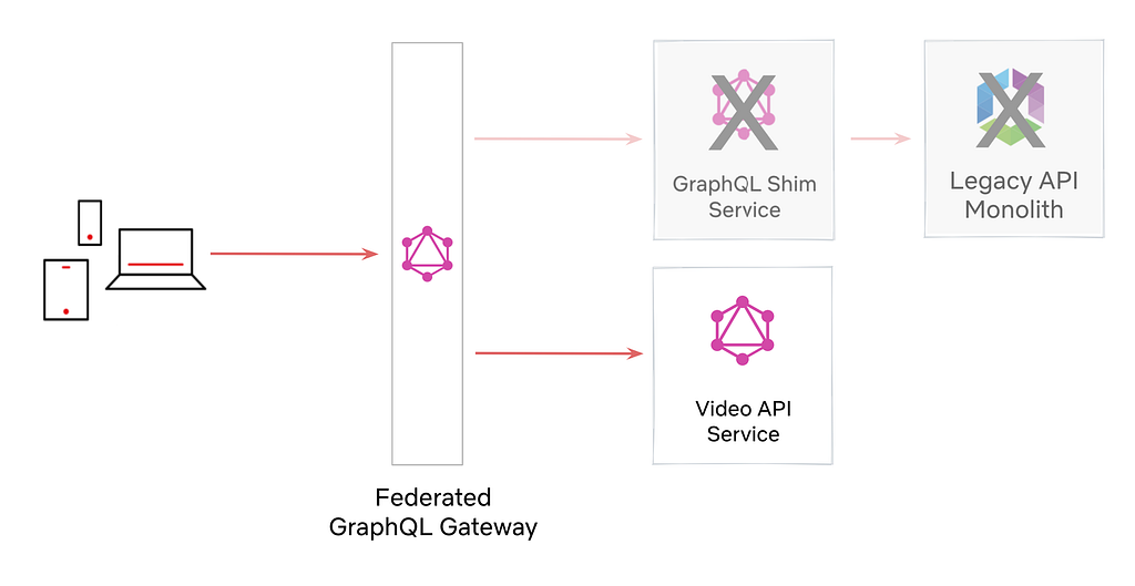
Until recently, an internal API framework, Falcor, powered our mobile apps. They are now backed by Federated GraphQL, a distributed approach to APIs where domain teams can independently manage and own specific sections of the API.

Doing this safely for 100s of millions of customers without disruption is exceptionally challenging, especially considering the many dimensions of change involved. This blog post will share broadly-applicable techniques (beyond GraphQL) we used to perform this migration. The three strategies we will discuss today are AB Testing, Replay Testing, and Sticky Canaries.

Migration Details

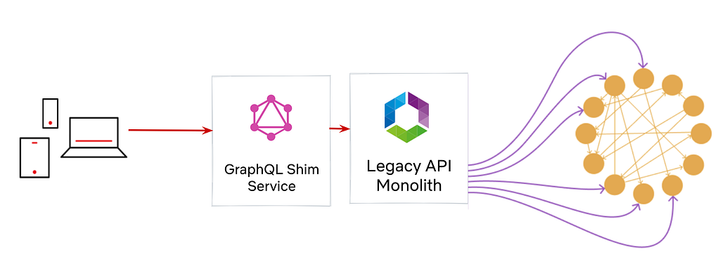
Before diving into these techniques, let’s briefly examine the migration plan.

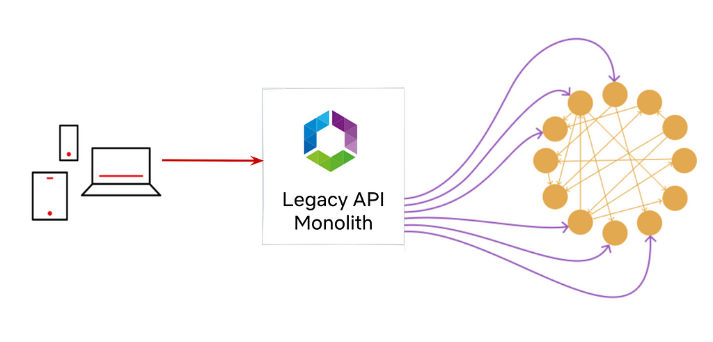
Before GraphQL: Monolithic Falcor API implemented and maintained by the API Team

Before moving to GraphQL, our API layer consisted of a monolithic server built with Falcor. A single API team maintained both the Java implementation of the Falcor framework and the API Server.

Phase 1

Created a GraphQL Shim Service on top of our existing Monolith Falcor API.

By the summer of 2020, many UI engineers were ready to move to GraphQL. Instead of embarking on a full-fledged migration top to bottom, we created a GraphQL shim on top of our existing Falcor API. The GraphQL shim enabled client engineers to move quickly onto GraphQL, figure out client-side concerns like cache normalization, experiment with different GraphQL clients, and investigate client performance without being blocked by server-side migrations. To launch Phase 1 safely, we used AB Testing.

Phase 2

Deprecate the GraphQL Shim Service and Legacy API Monolith in favor of GraphQL services owned by the domain teams.

We didn’t want the legacy Falcor API to linger forever, so we leaned into Federated GraphQL to power a single GraphQL API with multiple GraphQL servers.

We could also swap out the implementation of a field from GraphQL Shim to Video API with federation directives. To launch Phase 2 safely, we used Replay Testing and Sticky Canaries.

Testing Strategies: A Summary

Two key factors determined our testing strategies:

  • Functional vs. non-functional requirements
  • Idempotency

If we were testing functional requirements like data accuracy, and if the request was idempotent, we relied on Replay Testing. We knew we could test the same query with the same inputs and consistently expect the same results.

We couldn’t replay test GraphQL queries or mutations that requested non-idempotent fields.

And we definitely couldn’t replay test non-functional requirements like caching and logging user interaction. In such cases, we were not testing for response data but overall behavior. So, we relied on higher-level metrics-based testing: AB Testing and Sticky Canaries.

Let’s discuss the three testing strategies in further detail.

Tool: AB Testing

Netflix traditionally uses AB Testing to evaluate whether new product features resonate with customers. In Phase 1, we leveraged the AB testing framework to isolate a user segment into two groups totaling 1 million users. The control group’s traffic utilized the legacy Falcor stack, while the experiment population leveraged the new GraphQL client and was directed to the GraphQL Shim. To determine customer impact, we could compare various metrics such as error rates, latencies, and time to render.

We set up a client-side AB experiment that tested Falcor versus GraphQL and reported coarse-grained quality of experience metrics (QoE). The AB experiment results hinted that GraphQL’s correctness was not up to par with the legacy system. We spent the next few months diving into these high-level metrics and fixing issues such as cache TTLs, flawed client assumptions, etc.

Wins

High-Level Health Metrics: AB Testing provided the assurance we needed in our overall client-side GraphQL implementation. This helped us successfully migrate 100% of the traffic on the mobile homepage canvas to GraphQL in 6 months.

Gotchas

Error Diagnosis: With an AB test, we could see coarse-grained metrics which pointed to potential issues, but it was challenging to diagnose the exact issues.

Tool: Replay Testing — Validation at Scale!

The next phase in the migration was to reimplement our existing Falcor API in a GraphQL-first server (Video API Service). The Falcor API had become a logic-heavy monolith with over a decade of tech debt. So we had to ensure that the reimplemented Video API server was bug-free and identical to the already productized Shim service.

We developed a Replay Testing tool to verify that idempotent APIs were migrated correctly from the GraphQL Shim to the Video API service.

How does it work?

The Replay Testing framework leverages the @override directive available in GraphQL Federation. This directive tells the GraphQL Gateway to route to one GraphQL server over another. Take, for instance, the following two GraphQL schemas defined by the Shim Service and the Video Service:

The GraphQL Shim first defined the certificationRating field (things like Rated R or PG-13) in Phase 1. In Phase 2, we stood up the VideoService and defined the same certificationRating field marked with the @override directive. The presence of the identical field with the @override directive informed the GraphQL Gateway to route the resolution of this field to the new Video Service rather than the old Shim Service.

The Replay Tester tool samples raw traffic streams from Mantis. With these sampled events, the tool can capture a live request from production and run an identical GraphQL query against both the GraphQL Shim and the new Video API service. The tool then compares the results and outputs any differences in response payloads.

Note: We do not replay test Personally Identifiable Information. It’s used only for non-sensitive product features on the Netflix UI.

Once the test is completed, the engineer can view the diffs displayed as a flattened JSON node. You can see the control value on the left side of the comma in parentheses and the experiment value on the right.

/data/videos/0/tags/3/id: (81496962, null)
/data/videos/0/tags/5/displayName: (Série, value: “S\303\251rie”)

We captured two diffs above, the first had missing data for an ID field in the experiment, and the second had an encoding difference. We also saw differences in localization, date precisions, and floating point accuracy. It gave us confidence in replicated business logic, where subscriber plans and user geographic location determined the customer’s catalog availability.

Wins

  • Confidence in parity between the two GraphQL Implementations
  • Enabled tuning configs in cases where data was missing due to over-eager timeouts
  • Tested business logic that required many (unknown) inputs and where correctness can be hard to eyeball

Gotchas

  • PII and non-idempotent APIs should not be tested using Replay Tests, and it would be valuable to have a mechanism to prevent that.
  • Manually constructed queries are only as good as the features the developer remembers to test. We ended up with untested fields simply because we forgot about them.
  • Correctness: The idea of correctness can be confusing too. For example, is it more correct for an array to be empty or null, or is it just noise? Ultimately, we matched the existing behavior as much as possible because verifying the robustness of the client’s error handling was difficult.

Despite these shortcomings, Replay Testing was a key indicator that we had achieved functional correctness of most idempotent queries.

Tool: Sticky Canary

While Replay Testing validates the functional correctness of the new GraphQL APIs, it does not provide any performance or business metric insight, such as the overall perceived health of user interaction. Are users clicking play at the same rates? Are things loading in time before the user loses interest? Replay Testing also cannot be used for non-idempotent API validation. We reached for a Netflix tool called the Sticky Canary to build confidence.

A Sticky Canary is an infrastructure experiment where customers are assigned either to a canary or baseline host for the entire duration of an experiment. All incoming traffic is allocated to an experimental or baseline host based on their device and profile, similar to a bucket hash. The experimental host deployment serves all the customers assigned to the experiment. Watch our Chaos Engineering talk from AWS Reinvent to learn more about Sticky Canaries.

In the case of our GraphQL APIs, we used a Sticky Canary experiment to run two instances of our GraphQL gateway. The baseline gateway used the existing schema, which routes all traffic to the GraphQL Shim. The experimental gateway used the new proposed schema, which routes traffic to the latest Video API service. Zuul, our primary edge gateway, assigns traffic to either cluster based on the experiment parameters.

We then collect and analyze the performance of the two clusters. Some KPIs we monitor closely include:

  • Median and tail latencies
  • Error rates
  • Logs
  • Resource utilization–CPU, network traffic, memory, disk
  • Device QoE (Quality of Experience) metrics
  • Streaming health metrics

We started small, with tiny customer allocations for hour-long experiments. After validating performance, we slowly built up scope. We increased the percentage of customer allocations, introduced multi-region tests, and eventually 12-hour or day-long experiments. Validating along the way is essential since Sticky Canaries impact live production traffic and are assigned persistently to a customer.

After several sticky canary experiments, we had assurance that phase 2 of the migration improved all core metrics, and we could dial up GraphQL globally with confidence.

Wins

Sticky Canaries was essential to build confidence in our new GraphQL services.

  • Non-Idempotent APIs: these tests are compatible with mutating or non-idempotent APIs
  • Business metrics: Sticky Canaries validated our core Netflix business metrics had improved after the migration
  • System performance: Insights into latency and resource usage help us understand how scaling profiles change after migration

Gotchas

  • Negative Customer Impact: Sticky Canaries can impact real users. We needed confidence in our new services before persistently routing some customers to them. This is partially mitigated by real-time impact detection, which will automatically cancel experiments.
  • Short-lived: Sticky Canaries are meant for short-lived experiments. For longer-lived tests, a full-blown AB test should be used.

In Summary

Technology is constantly changing, and we, as engineers, spend a large part of our careers performing migrations. The question is not whether we are migrating but whether we are migrating safely, with zero downtime, in a timely manner.

At Netflix, we have developed tools that ensure confidence in these migrations, targeted toward each specific use case being tested. We covered three tools, AB testing, Replay Testing, and Sticky Canaries that we used for the GraphQL Migration.

This blog post is part of our Migrating Critical Traffic series. Also, check out: Migrating Critical Traffic at Scale (part 1, part 2) and Ensuring the Successful Launch of Ads.


Migrating Netflix to GraphQL Safely was originally published in Netflix TechBlog on Medium, where people are continuing the conversation by highlighting and responding to this story.

AWS Professional Services scales by improving performance and democratizing data with Amazon QuickSight

Post Syndicated from Ameya Agavekar original https://aws.amazon.com/blogs/big-data/aws-professional-services-scales-by-improving-performance-and-democratizing-data-with-amazon-quicksight/

The AWS Professional Services (ProServe) Insights team builds global operational data products that serve over 8,000 users within Amazon. Our team was formed in 2019 as an informal group of four analysts who supported ad hoc analysis for a division of ProServe consultants. ProServe is responsible for assisting enterprises as they shift to the cloud by incorporating Amazon Web Services (AWS) into their overall architecture. In recent years, the demand for domain expertise (ProServe) grew as various industries and organizations accelerated the move to the cloud.

We work hand in hand with customer teams and AWS partners to provide deep expertise in the architecture, design, development, and implementation of cloud computing initiatives that result in real business outcomes.

As our organization grew rapidly, we built new tools to scale analytical insights into our customers’ sales and delivery mechanisms. We were frustrated by the limitations of our previous business intelligence (BI) solution, which was holding us back from our vision to accelerate data sharing, team collaboration, and security within Amazon. To scale and continue innovating, we developed a secure Amazon QuickSight environment for our internal customers.

In this post, we discuss how QuickSight has helped us improve our performance, democratize our data, and provide insights to our internal customers at scale.

Enabling teams to build their own analyses at scale

The Insights team builds dashboards and supports thousands of internal consultants and hundreds of analysts and engineers across the globe who drive local products and insights. As a team of engineers focused on building a single source of truth within Amazon, we wanted a BI tool that was cost-effective, secure, and integrated seamlessly with the other AWS services we use. ProServe team members need to make strategic decisions on behalf of customers, and we play a key role by providing the tools they need to make the right decisions. We’ve made a big impact with QuickSight because it doesn’t require in-depth knowledge about data visualizations to build dashboards and provide insights, empowering our users to build what they need.

Our QuickSight instance is secure and tailored to use the Amazon active directory framework. We also helped 13 Amazon teams to set up their own instances. The teams we serve have benefited from our switch to QuickSight. For example, AWS Professional Services launched Financial Insights Tool (FIT) 2 years ago, a QuickSight dashboard that reports project financials, project revenue leakage, and margin erosion by evaluating actuals and forecasts at any granularity. FIT saves 30 minutes per project per Engagement Manager (EM) per week, and securely centralizes project financials into a scalable tool. This empowers EMs to avoid building disparate local reporting that creates logic inconsistencies and data security issues.

One of our ProServe teams has 19 dashboards on QuickSight, including Catalog, Trend and Analysis, KPI Monitoring, Business Management, and Quality Control. In 2022, one of the KPI Monitoring dashboards helped save at least 5,600 hours in total across 230 managers and 2,000 consultants. Last year, this team also reported over 29,600 distinct views on their 19 dashboards.

Additionally, we launched the first iteration of a hygiene dashboard in February 2022. This dashboard helps our operations team and end customers improve the data quality of key attribution and reduce manual intervention. The hygiene dashboard makes sure all the checks are enabled to safely promote customer outcomes with better planning and forecasting capabilities. The adoption of the dashboard led to a 73% reduction in hygiene issues from February 2022 to February 2023. We attribute this reduction to better inspection from weekly business reviews, and with this dashboard as an inspection tool delivered via email subscription to our stakeholders.

Improved performance and flexibility

To onboard a new reader or author on our previous BI tool, we had to provide a new license each time. This manual process was time-consuming and costly. The QuickSight usage-based pricing model makes sure that we can provide analytics and insights to all users without the need to pay ahead for user-specific licenses. QuickSight guarantees that we can provide everyone access by default, enabling data democratization in ways we couldn’t before. Since moving to QuickSight, we have scaled from 1,400 licenses to over 8,000 unique viewers, thanks to its auto scaling capability. QuickSight is fully managed, serverless, and can automatically scale to tens of thousands of users without any infrastructure to manage or capacity to plan for.

We used to have to track our dashboard loading times on our previous tool, but QuickSight has made that a thing of the past. With QuickSight SPICE (Super-fast, Parallel, In-memory Calculation Engine), our dashboards load in seconds, not minutes. Our high impact dashboards for ProServe weekly business reviews, utilization and time card deep dive, and impact points use the powerful SPICE functionality, which has support for up to 1 billion rows.

The Weekly Business Review (WBR) Backlog Summary dashboard that replaced the complex scorecards with interactive QuickSight visuals:

Implementing the FAIRS data sharing framework

QuickSight improves the ability to securely Find, Access, Interoperate, and Reuse (FAIRS) the data across ProServe, AWS, and Amazon. This framework can be described as follows:

  • Findable – Metadata and data should be easy to find for both humans and computers. All datasets and dashboards in the same account provide us an opportunity to see the big picture. This streamlines the reports’ and dashboards’ dictionary-building process for ProServe. Automatic discovery of datasets, reports, and dashboards improves the analytical community’s efficiency and productivity.
  • Accessible – Users need to be able to access the data they need easily and securely. In our case, we can control the access using appropriate roles, groups, and highly secure authentication methods not only for users but also for our data sources, datasets, and dashboards using Amazon Active Directory Connected Groups.
  • Interoperable – As the worldwide central team across 10 geographies and over 2,000 practices, our data needs to interoperate with applications or workflows for analysis, storage, and processing. This allows many different parts of the organization to collaborate as a cohesive unit.
  • Reusable – The ultimate goal of FAIRS is to optimize the reuse of data. To achieve this, metadata and data should be well-described so that they can be replicated or combined in different settings. This way, we can save time and focus our analysis on diving deeper into the insights.
  • Security – Security is job Zero. We believe that everyone should have secure data access to make data-driven decisions. At ProServe, we use Amazon Active Directory, column-level security (CLS), and row-level security (RLS) to maintain the high bar in data security.

QuickSight has brought us closer to achieving FAIRS than we could get with our previous BI solution. Dashboards are easily searchable, highly collaborative, and secure.

The User Activities Tracking dashboard created by ProServe’s QuickSight administrators:

Seamless AWS Integration

QuickSight integrates seamlessly with other AWS services such as Amazon SageMaker to use machine learning insights within a low code or no code environment. Our users can simply connect to any of the QuickSight supported data sources—including Amazon Simple Storage Service (Amazon S3), Amazon Athena, Amazon Relational Database Service (Amazon RDS), and Amazon Redshift—and select the SageMaker model they want to use for prediction. QuickSight has also made it possible for dashboard development from non-analyst roles.

QuickSight is constantly evolving. Eighty-four features were added in 2022. One of those features is asset management, which has made it easier for us to transfer assets from one group to another to onboard new employees. With QuickSight, we have reached over 9,200 distinct viewers and over 500,000 total views at Amazon with 485 dashboards.

The Skills dashboard representing the percentage match of top 100 skills entered by each specialization:

QuickSight has enabled us to scale with the growth of our team without sacrificing our performance. Instead, we improved our performance and democratized our data, thanks to great capabilities such as SPICE, the flexibility of the product, and its seamless integration with the other AWS services. We look forward to continuing to provide solutions to our internal customers by exploring other QuickSight capabilities such as Amazon QuickSight Q, embedded analytics, and more.

To learn more about how QuickSight can help your business with dashboards, reports, and more, visit Amazon QuickSight.


About the Authors

Ameya Agavekar is a results-driven, highly skilled data strategist. Ameya leads the data engineering and data science function for AWS Professional Services World-Wide Business Insights & Analytics team. Outside of work, Ameya is a professional pilot. He enjoys serving community by applying his unique flying skills with the US Airforce auxiliary Civil Air Patrol.

Tucker Shouse leads the AWS Professional Services World-Wide Business Insights & Analytics team. Prior to AWS, Tucker worked with financial services, retail, healthcare, and non-profit clients to develop digital and data products and strategies as a Manager at Alvarez & Marsal Corporate Performance Improvement. Outside of work, Tucker enjoys spending time with his wife and daughter enjoying the outdoors and music.

Best practices for running production workloads using Amazon MSK tiered storage

Post Syndicated from Nagarjuna Koduru original https://aws.amazon.com/blogs/big-data/best-practices-for-running-production-workloads-using-amazon-msk-tiered-storage/

In the second post of the series, we discussed some core concepts of the Amazon Managed Streaming for Apache Kafka (Amazon MSK) tiered storage feature and explained how read and write operations work in a tiered storage enabled cluster.

This post focuses on how to properly size your MSK tiered storage cluster, which metrics to monitor, and the best practices to consider when running a production workload.

Sizing a tiered storage cluster

Sizing and capacity planning are critical aspects of designing and operating a distributed system. It involves estimating the resources required to handle the expected workload and ensure the system can scale and perform efficiently. In the context of a distributed system like Kafka, sizing involves determining the number of brokers, the number of partitions, and the amount of storage and memory required for each broker. Capacity planning involves estimating the expected workload, including the number of producers, consumers, and the throughput requirements.

Let’s assume a scenario where the producers are evenly balancing the load between brokers, brokers host the same number of partitions, there are enough partitions to ingest the throughput, and consumers consume directly from the tip of the stream. The brokers are receiving the same load and doing the same work. We therefore just focus on Broker1 in the following diagram of a data flow within a cluster.

Theoretical sustained throughput with tiered storage

We derive the following formula for the theoretical sustained throughput limit tcluster given the infrastructure characteristics of a specific cluster with tiered storage enabled on all topics:

max(tcluster) <= min {

max(tstorage) * #brokers/(r + 1 + #non_tip_local_consumer_groups),
max(tNetworkAttachedStorage) * #brokers/(r + 1 + #non_tip_local_consumer_groups),
max(tEC2network) * #brokers/(#tip_consumer_groups + r + #remote_consumer_groups)

}

This formula contains the following values:

  • tCluster – Total ingress produce throughput sent to the cluster
  • tStorage – Storage volume throughput supported
  • tNetworkAttachedStorage – Network attached storage to the Amazon Elastic Compute Cloud (Amazon EC2) instance network throughput
  • tEC2network – EC2 instance network bandwidth
  • non_tip_local_consumer_groups – Number of consumer groups reading from network attached storage at ingress rate
  • tip_consumer_groups – Number of consumer groups reading from page cache at ingress rate
  • remote_consumer_groups – Number of consumer groups reading from remote tier at ingress rate
  • r – Replication factor of the Kafka topic

Note that in the first post , we didn’t differentiate between different types of consumer groups. With tiered storage, some consumer groups might be consuming from remote. These remote consumers might ultimately catch up and start reading from local storage and finally catch up to the tip. Therefore, we model these three different consumer groups in the equation to account for their impact on infrastructure usage. In the following sections, we provide derivations of this equation.

Derivation of throughput limit from network attached storage bottleneck

Because Amazon MSK uses network attached storage for local storage, both network attached storage throughput and bandwidth should be accounted for. Total throughput bandwidth requirement is a combination of ingress and egress from the network attached storage backend. The ingress throughput of the storage backend depends on the data that producers are sending directly to the broker plus the replication traffic the broker is receiving from its peers. With tiered storage, Amazon MSK also uses network attached storage to read and upload rolled segments to the remote tier. This doesn’t come from the page cache and needs to be accounted for at the rate of ingress. Any non-tip consumers at ingress rate also consume network attached storage throughput and are accounted for in the equation. Therefore, max throughput is bounded by network attached storage based on the following equation:

max(tcluster) <= min {

max(tstorage) * #brokers/(r + 1 + #non_tip_local_consumer_groups),
max(tNetworkAttachedStorage) * #brokers/(r + 1 + #non_tip_local_consumer_groups)

}

Derivation of throughput limit from EC2 network bottleneck

Unlike network attached storage, the network is full duplex, meaning that if the EC2 instance supports X MB/s network, it supports X MB/s in and X MB/s out. The network throughput requirement depends on the data that producers are sending directly to the broker plus the replication traffic the broker is receiving from its peers. It also includes the replication traffic out and consumers traffic out from this broker. With tiered storage, we need to reserve additional ingress rate for uploads to the remote tier and support reads from the remote tier for consumer groups reading from remote offset. Both of these add to the network out requirements, which is bounded by the following equation:

max(tcluster) <= min {

max(tEC2network) * #brokers/(#tip_consumer_groups + r + #remote_consumer_groups)

}

Combining the second and third equations provides the first formula, which determines the max throughput bound based on broker infrastructure limits.

How to apply this formula to size your cluster

With this formula, you can calculate the upper bound for throughput you can achieve for your workloads. In practice, the workloads may be bottlenecked by other broker resources like CPU, memory, and disk, so it’s important to do load tests. To simplify your sizing estimate, you can use the MSK Sizing and Pricing spreadsheet (for more information, refer to Best Practices).

Let’s consider a workload where your ingress and egress rates are 20MB/s, with a replication factor of 3, and you want to retain data in your Kafka cluster for 7 days. This workload requires 6x m5.large brokers, with 34.6 TB local storage, which will cost $6,034.00 monthly (estimated). But if you use tiered storage for the same workload with local retention of 4 hours and overall data retention of 7 days, it requires 3x m5.large brokers, with 0.8 TB local storage and 12 TB of tiered storage, which will cost $1,958.00 monthly(estimated). If you want to read all the historic data one time, it will cost $17.00 ($0.0015 per GB retrieval cost). In this example with tiered storage, you save around 67.6% of your overall cost.

We recommend planning for Availability Zone redundancy in production workloads considering the broker safety factor in the calculation, which is 1 in this example. We also recommend running performance tests to ensure CPU is less than 70% on your brokers at the target throughput derived based on this formula or Excel calculation. In addition, you should also use the per-broker partition limit in your calculation to account for other bottlenecks based on the partition count.

The following figure shows an example of Amazon MSK sizing.

Monitoring and continuous optimization for a tiered storage enabled cluster

In previous sections, we emphasized the importance of determining the correct initial cluster size. However, it’s essential to recognize that sizing efforts shouldn’t cease after the initial setup. Continual monitoring and evaluation of your workload are necessary to ensure that the broker size remains appropriate. Amazon MSK offers metric monitoring and alarm capabilities to provide visibility into cluster performance. In the post Best practices for right-sizing your Apache Kafka clusters to optimize performance and cost, we discussed key metrics to focus on. In this post, we delve deeper into additional metrics related to tiered storage and other optimization considerations for a tiered storage enabled cluster:

  • TotalTierBytesLag indicates the total number of bytes of the data that is eligible for tiering on the broker and hasn’t been transferred to the tiered storage yet. This metric shows the efficiency of upstream data transfer. As the lag increases, the amount of data that hasn’t yet persisted in the tiered storage increases. The impact is the network attached storage disk may fill up, which you should monitor. You should also monitor this metric and generate an alarm if the lag is continuously growing and you see increased network attached storage usage. If the tiering lag is too high, you can reduce ingress traffic to allow the tiered storage to catch up.
  • Although tiered storage provides on-demand, virtually unlimited storage capacity without provisioning any additional resources, you should still do proper capacity planning for your local storage, configure alerts for KafkaDataLogsDiskUsed metrics, and have a buffer on network attached storage capacity planning. Monitor this metric and generate an alarm if the metric reaches or exceeds 60%. For a tiered storage enabled topic, configure local retention accordingly to reduce network attached storage usage.
  • The theoretical max ingress we can achieve on an MSK cluster with tiered storage is 20–25% lower than a non-tiered storage enabled cluster due to additional network attached storage bandwidth required to transparently move data from the local to the remote tier. Plan for the capacity (brokers, storage, gp2 vs. gp3) using the formula we discussed to derive max ingress for your cluster based on the number of consumer groups and load test your workloads to identify the sustained throughput limit. Exercising excess ingress to the cluster or egress from the remote tier above the planned capacity can impact your tip produce or consume traffic.
  • The gp3 volume type offers SSD-performance at a 20% lower cost per GB than gp2 volumes. Furthermore, by decoupling storage performance from capacity, you can easily provision higher IOPS and throughput without the need to provision additional block storage capacity. Therefore, we recommend using gp3 for a tiered storage enabled cluster by specifying provisioned throughput for larger instance types.
  • If you specified a custom cluster configuration, check the num.replica.fetchers, num.io.threads, and num.network.threads configuration parameters on your cluster. We recommend leaving it as the default Amazon MSK configuration unless you have specific use case.

This is only the most relevant guidance related to tiered storage. For further guidance on monitoring and best practices of your cluster, refer to Best practices.

Conclusion

You should now have a solid understanding of how Amazon MSK tiered storage works and the best practices to consider for your production workload when utilizing this cost-effective storage tier. With tiered storage, we remove the compute and storage coupling, which can benefit workloads that need larger disk capacity and are underutilizing compute just to provision storage.

We are eager to learn about your current approach in building real-time data streaming applications. If you’re starting your journey with Amazon MSK tiered storage, we suggest following the comprehensive Getting Started guide available in Tiered storage. This guide provides detailed instructions and practical steps to help you gain hands-on experience and effectively take advantage of the benefits of tiered storage for your streaming applications.

If you have any questions or feedback, please leave them in the comments section.


About the authors

Nagarjuna Koduru is a Principal Engineer in AWS, currently working for AWS Managed Streaming For Kafka (MSK). He led the teams that built MSK Serverless and MSK Tiered storage products. He previously led the team in Amazon JustWalkOut (JWO) that is responsible for realtime tracking of shopper locations in the store. He played pivotal role in scaling the stateful stream processing infrastructure to support larger store formats and reducing the overall cost of the system. He has keen interest in stream processing, messaging and distributed storage infrastructure.

Masudur Rahaman Sayem is a Streaming Data Architect at AWS. He works with AWS customers globally to design and build data streaming architectures to solve real-world business problems. He specializes in optimizing solutions that use streaming data services and NoSQL. Sayem is very passionate about distributed computing.

Haas: The PostgreSQL Documentation and the Limitations of Community

Post Syndicated from original https://lwn.net/Articles/934674/

Robert Haas looks
at the advantages and disadvantages
of how documentation for PostgreSQL
is written.

The strengths of this process are also its weaknesses. A developer
is, by definition, someone who spends the majority of their time
doing development, which is to say writing code. Updating the
documentation becomes a task that must be completed so that the
code one has written can get committed so that one can move on to
the next project and write some more code. If a change to the
documentation would be beneficial but is unrelated to any
particular patch, it’s not likely to get done.

The results are, in a certain sense, pretty comical.

[$] Retrieving mount and filesystem information in user space

Post Syndicated from original https://lwn.net/Articles/934469/

In something of a follow-on from the mount-operation monitoring session the
previous day, Christian Brauner led another discussion about providing user
space with a mechanism to get current mount information on day two of the
2023 Linux Storage, Filesystem,
Memory-Management and BPF Summit
. The session also continued on from
one at last year’s
summit
—and likely others before that.
There are two separate proposals for ways to retrieve this kind of
information, one from Miklos Szeredi and another from David Howells, both
of whom were present this year; Brauner’s intent was to try to reach some
kind of agreement on the way forward in the session.

Disaster Recovery for Oracle Database on Amazon EC2 with Fast-Start Failover

Post Syndicated from Harshad Gohil original https://aws.amazon.com/blogs/architecture/disaster-recovery-for-oracle-database-on-amazon-ec2-with-fast-start-failover/

High availability is non-negotiable for organizations today to prevent business-critical application disruptions. Enterprises must prioritize database scalability and availability to avoid downtime in their databases, network, servers, or storage environments.

For organizations that want to avoid required application changes, Oracle Real Application Clusters (RAC) is an option for providing high availability and scalability to the Oracle database. While the RAC feature is not supported by Oracle databases on Amazon Elastic Compute Cloud (Amazon EC2), Oracle Active Data Guard helps achieve high availability on AWS cloud.

The Oracle Data Guard feature helps customers survive disasters and data corruption while creating, maintaining, and managing one or more synchronized standby databases. But further, configuring Oracle Data Guard Fast-Start Failover (FSFO) helps achieve high availability.

In this blog post, we provide an architectural solution to achieve database high availability when running Oracle Database on Amazon EC2 with Oracle Data Guard along with Fast-Start Failover to address Availability Zones (AZs) or Amazon EC2 instance failures. We also introduce the steps you can take to make database failover happen without manual intervention, and offer recommendations for cross-Region disaster recovery.

Solution overview

Let’s explore this solution by discussing the architecture and two alternate options for securing high availability using Oracle Data Guard, along with the advantages and limitations of each. We will then offer a walkthrough of steps to make database failover happen without manual intervention.

Oracle high availability using Oracle Data Guard with multi-AZ and multi-Region with multi-AZ setup

This architecture is recommended to maintain high availability for Oracle databases on Amazon EC2 with protection against Amazon EC2 service outages in a Region. A disaster recovery environment and higher resiliency are provided after an Amazon EC2 service outage. This protects against Amazon EC2 service outages in an AWS Region and maintains resiliency due to the multi-AZ setup in a secondary Region.

In this architecture, Oracle Data Guard Fast Sync replication exists between the Primary database in AZ 1 in Region A, with standbys in AZ 2 Region A (Fast Sync), AZ1 in Region B (ASYNC), and AZ2 in Region B (ASYNC). There is an asynchronous cascading replication setup between standby databases to avoid network latency issues across regions.

Should Region A experience an Amazon EC2 service outage, the Oracle observer, a client software that monitors Oracle Data Guard and initiate failover to the Standby database in Region B. Applications can continue to connect to the database resulting in high availability with limited/minimal data loss based on the data change rate amount, as in Figure 1.

Oracle with cascading standby databases across regions

Figure 1. Oracle with cascading standby databases across regions

Using Oracle RedoRoutes, the default behavior of Data guard can be controlled and it can be set using the following example during setup.

Oracle RedoRoutes setup example:

dgmgrl > edit database DB_1A set property RedoRoutes= ‘ (LOCAL: DB_1B FASTSYNC PRIORITY=1, DB_2A ASYNC PRIORITY=2,DB_2B ASYNC PRIORITY=3)) (DB_1B: (DB_2A ASYNC PRIORITY=1, DB_2B ASYNC PRIORITY=2)) (DB_2A: DB_1B ASYNC) (DB_2B: DB_1B ASYNC)’

dgmgrl > edit database DB_1B set property RedoRoutes= ‘(LOCAL: (DB_1A FASTSYNC PRIORITY=1, DB_2A ASYNC PRIORITY=2,DB_2B ASYNC PRIORITY=3))(DB_1A: (DB_2A ASYNC PRIORITY=1, DB_2B ASYNC PRIORITY=2)) ‘

dgmgrl > edit database DB_1B set property RedoRoutes= ‘(LOCAL: (DB_2B FASTSYNC PRIORITY=1, DB_1A ASYNC PRIORITY=2, DB_1B ASYNC PRIORITY=3))(DB_2B: (DB_1A ASYNC PRIORITY=1, DB_1B ASYNC PRIORITY=2)) (DB_1A: DB_2B ASYNC)(DB_1B: DB_2B ASYNC )’

dgmgrl > edit database DB_1B set property RedoRoutes= ‘(LOCAL: (DB_2A FASTSYNC PRIORITY=1, DB_1A ASYNC PRIORITY=2, DB_1B ASYNC PRIORITY=3))(DB_2A: (DB_1A ASYNC PRIORITY=1, DB_1B ASYNC PRIORITY=2))’

For more information on Oracle RedoRoutes setup for Oracle Cascading Standby, refer to this step-by-step configuration documentation.

Database failover with Amazon Route 53 and Oracle Data Guard

The following walkthrough defines the steps you can take to make database failover happen without manual intervention using Amazon Route 53 and Oracle Data Guard.

Prerequisites

Before getting started, review the following prerequisites for this solution:

Walkthrough

Step 1. Create Oracle Database Service

For applications to connect without manual intervention on event of failure, we recommend creating an Oracle database service using the Oracle DBMS_Package called DBMS_SERVICE.

exec dbms_service.CREATE_SERVICE(SERVICE_NAME=>'DB_SERVICE_FOR_APP', NETWORK_NAME=>'DB_SERVICE_FOR_APP');

exec dbms_service.START_SERVICE('DB_SERVICE_FOR_APP');

Step 2. Network configuration

Applications can connect to the database seamlessly without manual intervention in an event of a failover from the Primary database to Standby using the Oracle Transparent Application Failover (TAF) approach, though TAF requires updating application connection strings in case of a host IP change.

The following approach using Amazon Route 53 is recommended for added flexibility and scalability. Route 53 has DNS A records that map to the database instance IPs and CNAME records that can redirect DNS queries to A records. The following depicts the DNS mapping. The CNAME, along with the database service name, can be used by the application in its network configuration.

Database_Name =
 (DESCRIPTION =
    (ADDRESS_LIST =
       (ADDRESS = (PROTOCOL = TCP)(HOST = <db_cname>)(PORT = 1521))
   (connect_data = 
       (service_name = <db_service_name>)
   )) )

To update the CNAME in Route 53 to map to the Primary host automatically in the event of failure, follow these steps.

Step 3. Route 53 setup

Create a script named route53update.sh and place it on the database hosts using the following code.

#!/bin/bash

export ORACLE_HOME="<<change>> "

export LD_LIBRARY_PATH=$ORACLE_HOME/lib

export PATH=$ORACLE_HOME/bin:$PATH:/usr/local/bin:/usr/bin

LOG_FILE="/tmp/switch_dns_$$.log"

DNS_DOMAIN="<<change>> "

ACTIVE_DB_CNAME="<<change>> "

HOSTED_ZONE_ID="<<change>> "

TTL="<<change>> "

update_dns () {

TMPFILE="/tmp/route53_dns_$$.log"

 cat > ${TMPFILE} << EOF

    {

      "Comment":"Updating DNS of record ${1}.${DNS_DOMAIN}",

      "Changes":[

        {

          "Action":"UPSERT",

          "ResourceRecordSet":{

            "ResourceRecords":[

              {

                "Value":"$2"

              }

            ],

            "Name":"${1}.${DNS_DOMAIN}.",

            "Type":"CNAME",

            "TTL":$TTL

          }

        }

      ]

    }

EOF

  /usr/local/bin/aws route53 change-resource-record-sets \

        --hosted-zone-id $HOSTED_ZONE_ID \

        --change-batch file://"$TMPFILE" >> "$LOG_FILE"

}

prim_uniq_sid=`$ORACLE_HOME/bin/sqlplus -s  / as sysdba <<EOF

set feedback off echo off lines 2000 head off

select upper(db_unique_name) from  v\\$dataguard_config where DEST_ROLE='PRIMARY DATABASE';

EOF`

prim_uniq_sid=`echo $prim_uniq_sid| sed 's/^[ \t]*//;s/[ \t]*$//'`

host_current=`$ORACLE_HOME/bin/tnsping ${prim_uniq_sid}|sed -n 's/\(.*Host\)\([^)]*\)\(.*\)/\2/pi' |sed 's/=//g'|sed 's/^[ \t]*//;s/[ \t]*$//'`

dns_current_host=`/usr/local/bin/aws route53 list-resource-record-sets --hosted-zone-id $HOSTED_ZONE_ID --query  "ResourceRecordSets[?Name == '${ACTIVE_DB_CNAME}.${DNS_DOMAIN}.'].ResourceRecords" --output text`

if [ "$host_current" != "$dns_current_host" ]; then

        update_dns ${ACTIVE_DB_CNAME} $host_current

fi

Step 4. Database job setup

Create a job in the Oracle Primary database to execute the shell script just introduced to initiate in the event of failover using the following code.

begin
  dbms_scheduler.create_job
  (
    job_name             => 'route53update',
    job_type             => 'executable',
    number_of_arguments  => 0,
    job_action           => '/<<location of script>>/ route53update.sh',
    auto_drop            => false
  );

  dbms_scheduler.enable('route53update');
end;
/

Step 5. Database trigger setup

In an event of a failure, the Primary will failover and the Standby starts up as the new Primary. A trigger needs to be created on the Primary database to execute the job on any failover to update the Route53 CNAME using the following code.

create or replace trigger SYS.Update_Route53_Record
AFTER STARTUP ON DATABASE
DECLARE
db_role varchar2(16);
db_mode varchar2(20);BEGIN
select database_role, open_mode into db_role, db_mode from v$database;
if db_role = 'PRIMARY' then
dbms_scheduler.run_job('route53update') ;
END IF;
END;
/

Alternate Option 1: Single Region with multi-AZ

This option is a minimum recommended configuration to maintain high availability for Oracle databases on Amazon EC2 for customers who do not have a multi-region setup.

  • Advantage: Protects against Amazon EC2 service outage in a single AZ.
  • Limitation: Does not protect against Amazon EC2 service outages in a single Region.

In this architecture, Oracle Data Guard Fast Sync replication exists between the Oracle database instance in a multi-AZ setup with the Primary database (Read Write) in AZ 1 and the Standby database (Read Only) in AZ 2.

If the primary database is unreachable due to any failure, the observer will failover to the standby database in a different AZ. Applications can continue to connect to the database with zero data loss due to synchronous replication between AZ using the Maximum Availability/Maximum Protection mode setup in Oracle Data Guard. If the primary database is in us-east-1a and standby in us-east-1b, the RedoRoutes property can be defined as follows.

Oracle RedoRoutes setup example:

dgmgrl> edit database DB_1A set property RedoRoutes= '(LOCAL: (DB_1B FASTSYNC)'

dgmgrl>  edit database DB_1B set property RedoRoutes= '(LOCAL: (DB_1A FASTSYNC)'

For more information on how disaster recovery works in the AWS Cloud, visit the Disaster recovery is different in the cloud section of the AWS Well-Architected Framework. For more on Oracle RedoRoutes setup, refer to the Oracle Redo Routing Rules documentation.

Alternate Option 2: Multi-AZ with multi-Region with single AZ

This option is recommended to maintain high availability for an Oracle database on Amazon EC2 for customers who need multi-region availability. It provides protection against the rare unavailability of Amazon EC2 instances in the primary Region, in which case a disaster recovery environment is provided.

  • Advantage: Protects against Amazon EC2 service outages in a 2 AZ or AWS Region.
  • Limitation: Decreased resiliency without high availability on Amazon EC2 service outage in an entire Region

In this architecture, Oracle Data Guard Fast Sync replication exists between the Oracle database instance in multi-AZ within the single Region, with the Primary database in AZ 1 in Region A and Standby database in AZ 2 in Region A. There is an asynchronous replication setup between the Standby database cross-Region.

Asynchronous replication is recommended between Region replication to avoid network latency issue. A cascading standby setup ensures there is no additional performance impact on the primary database to send data to multiple standbys.

If the primary database is unreachable, failover happens between AZs in Region A. In the event of an Amazon EC2 service outage in a Region, failover occurs to Region B, resulting in high availability with minimal data loss based on the data change rate amount. If the primary database is in us-east-1a and standby in us-east-1b (Fast Sync) and us-east-2a (Async), the RedoRoutes property can be defined as follows.

Oracle RedoRoutes setup example:

dgmgrl > edit database DB_1A set property RedoRoutes= '(LOCAL: (DB_1B FASTSYNC PRIORITY=1, DB_2A ASYNC PRIORITY=2))(DB_1B: DB_2A ASYNC)(DB_2A: DB_1B ASYNC)'

dgmgrl > edit database DB_1B set property RedoRoutes= '(LOCAL: (DB_1A FASTSYNC PRIORITY=1, DB_2A ASYNC  PRIORITY=2)) (DB_1A: DB_2A ASYNC)'

dgmgrl > edit database DB_1B set property RedoRoutes= '(LOCAL: (DB_1A FASTSYNC PRIORITY=1, DB_1B ASYNC  PRIORITY=2))'

Cleaning up

The services involved in this solution incur costs. When you’re done using this solution, clean up the following resources:

  • Amazon EC2 instances – Stop or delete (terminate) the Amazon EC2 instances that you provisioned.
  • Route53 – Delete the hosted Zone ID and A records/CNAMEs created.

Conclusion

This blog post demonstrates how high availability and disaster recovery can be achieved for an Oracle database on an Amazon EC2 instance using Oracle Data Guard. Using the architectures in this post, you can achieve zero data loss with the Oracle Fast-Start Failover option within the same Region or cross-Region on Amazon EC2.

You can also use this architecture to replicate data from an Oracle database on Amazon EC2 to an Oracle database hosted outside of the AWS cloud. With Oracle Cascading Standby and Oracle RedoRoutes, you can remove high dependency on the Primary database to improve overall performance.

[$] Hardening magic links

Post Syndicated from original https://lwn.net/Articles/934460/

There are some “magic links” in kernel pseudo-filesystems, like procfs,
that can be—have been—(ab)used to cause security problems, such as a
container-confinement breach in 2019.
Aleksa Sarai has long been working on ways to blunt the impact of these
magic links. He led a filesystem session at the
2023 Linux Storage, Filesystem,
Memory-Management and BPF Summit
to discuss the status of those efforts.

Simplify fine-grained authorization with Amazon Verified Permissions and Amazon Cognito

Post Syndicated from Phil Windley original https://aws.amazon.com/blogs/security/simplify-fine-grained-authorization-with-amazon-verified-permissions-and-amazon-cognito/

AWS customers already use Amazon Cognito for simple, fast authentication. With the launch of Amazon Verified Permissions, many will also want to add simple, fast authorization to their applications by using the user attributes that they have in Amazon Cognito. In this post, I will show you how to use Amazon Cognito and Verified Permissions together to add fine-grained authorization to your applications.

Fine-grained authorization

With Verified Permissions, you can write policies to use fine-grained authorization in your applications. Policy-based access control helps you secure your applications without embedding complicated access control code in the application logic. Instead, you write policies that say who can take what actions on which resources, and you evaluate the policies by using the Verified Permissions API. The API evaluates access control policies in the context of an access request: Who’s making the request? What do they want to do? What do they want to access? Under what conditions are they making the request?

AWS has removed the work needed to create context about who is making the request by using data from Amazon Cognito. By using Amazon Cognito as your identity store and integrating Verified Permissions with Amazon Cognito, you can use the ID and access tokens that Amazon Cognito returns in the authorization decisions in your applications. You provide Amazon Cognito tokens to Verified Permissions, which uses the attributes that the tokens contain to represent the principal and identify the principal’s entitlements.

Make access requests

To write policies for Verified Permissions, you use a policy language called Cedar. The examples in this post are modified from those in the Cedar language tutorial; I recommend that you review this tutorial for a comprehensive introduction on how to build and use Cedar policies. The following is an example of what a Cedar policy in a photo-sharing application might look like:

permit(
  principal == User::"alice", 
  action    == Action::"update", 
  resource  == Photo::"VacationPhoto94.jpg"
);

This policy states that Alice—the principal—is permitted to update the resource named VacationPhoto94.jpg. You place the policies for your application in a dedicated policy store. To ask Verified Permissions for an authorization decision, use the isAuthorized operation from the API. For example, the following request asks if user alice is permitted to update VacationPhoto94.jpg. Note that I’ve left out details like the policy store identifier for clarity.

// JS pseudocode
const authResult = await avp.isAuthorized({
    principal: 'User::"alice"',
    action: 'Action::"update"',
    resource: 'Photo::"VacationPhoto94.jpg"'
});

This request returns a decision of allow because the principal, action, and resource all match those in the policy. If a user named bob tries to update the photo, the request returns a decision of deny because the policy only allows user alice. For requests that only need values for the principal, action, and resource, you can generally use values from the data in the application.

Things get more interesting when you build policies that use attributes of the principal to make the decision. In these cases, it can be challenging to assemble a complete and accurate authorization context. Policies might refer to attributes of the principal, such as their geographic location or whether they are paid subscribers. Fine-grained access control requires that you write good policies, properly format the access request, and provide the needed attributes for the policies to be evaluated. To get needed attributes, you must often make inline requests to other systems and then transform the results to meet the policy requirements.

The following policy uses an attribute requirement to allow any principal to view any resource as long as they are located in the United States.

permit(
  principal,
  action == Action::"view",
  resource
)
when {principal.location == "USA"};

To make an authorization request, you must supply the needed attributes for the principal. The following code shows how to do that by using the isAuthorized operation:

const authResult = await avp.isAuthorized({
    principal: 'User::"alice"',
    action: 'Action::"view"',
    resource: 'Photo::"VacationPhoto94.jpg"',
    // whenever our policy references attributes of the entity,
    // isAuthorized needs an entity argument that provides    
    // those attributes
    entities: [
        {
            "identifier": {
                "entityType": "User",
                "entityId": "alice"
            },
            "attributes": {
                "location": {
                    "String": "USA"
                }
            }
        ]
});

The authorization request now includes the context that Alice is located in the USA. According to the preceding policy, she should be allowed to view VacationPhoto94.jpg. To make this request, you must gather this information so that you can include it in the request.

Use Amazon Cognito

If the photo-sharing application uses Amazon Cognito for user authentication, then Amazon Cognito will pass an ID token to it when the authentication is successful. For more information about the format and encoding of ID tokens, see the OpenID Connect Core specification. For our purposes, it’s enough to know that after the ID token is verified and decoded, it contains a JSON structure with named attributes.

When you configure Amazon Cognito, you can specify the fields that are contained in the ID token. These might be user editable, but they can also be programmatically generated from other sources. Suppose that you have configured your Amazon Cognito user pool to also include a custom location attribute, custom:location. When Alice logs in to the photo-sharing application, the ID token that Amazon Cognito provides for her contains the following fields. Note that I’ve made the sub (subject) field human readable, but it would actually be a Amazon Cognito entity identifier.

{
 ...
 “iss”: “User”,
 “sub”: “alice”,
 “custom:location”: “USA”,
 ...
}

If the needed attributes are in Amazon Cognito, you can use them to create the attributes that isAuthorized needs to render an access decision.

Figure 1: Steps to use Amazon Cognito with isAuthorized

Figure 1: Steps to use Amazon Cognito with isAuthorized

As shown in Figure 1, you need to complete the following six steps to use isAuthorized with Amazon Cognito:

  1. Get the token from Amazon Cognito when the user authenticates
  2. Verify the token to authenticate the user
  3. Decode the token to retrieve attribute information
  4. Create the policy principal from information in the token or from other sources
  5. Create the entities structure by using information in the token or from other sources
  6. Call Amazon Verified Permissions by using isAuthorized

Now that you understand how to make a request by manually creating the context using data provided by an identity provider, I’ll share how the AWS integration of Amazon Cognito and Verified Permissions can help reduce your workload.

Use isAuthorizedWithToken

In addition to isAuthorized, the Verified Permissions API provides the isAuthorizedWithToken operation that accepts Amazon Cognito tokens. If your application uses Amazon Cognito for authentication, then Amazon Cognito provides the ID token after the user logs in. Let’s assume that you have stored this token in a variable named cognito_id_token. Because you are using an attribute from Amazon Cognito, you modify the previous policy to accommodate the namespace that the Amazon Cognito attributes are in, as shown in the following:

permit(
  principal,
  action == Action::"view",
  resource
)
when {principal.custom.location == "USA"};

With this policy, the photo-sharing application can use the ID token to make an authorization request using isAuthorizedWithToken:

Using this call, you don’t have to supply the principal or construct the entities argument for the principal. Instead, you just pass in the ID token that Amazon Cognito provides. When you call isAuthorizedWithToken, it constructs the principal by using information in the token and creates an entity context that includes Alice’s location from the attributes in the ID token.

Figure 2: Use isAuthorizedWithToken

Figure 2: Use isAuthorizedWithToken

As shown in Figure 2, when you use isAuthorizedWithToken, you only need to complete two steps:

  1. Get the token from Amazon Cognito when the user authenticates
  2. Call Verified Permissions using isAuthorizedWithToken, passing in the token

Optionally, your application might need to verify the token to authenticate the user and avoid unnecessary work, or it can rely on isAuthorizedWithToken to do that. Similarly, you might also decode the token if you need its values for the application logic.

Configure isAuthorizedWithToken

You can use the Verified Permissions console to tell the API which Amazon Cognito user pool you’re using for your application. This is called an identity source.

To create an identity source for use with Verified Permissions (console):

  1. Sign in to the AWS Management Console and open the Amazon Cognito console.
  2. Choose Identity source. You will see a list showing the sources that you have already configured.
  3. To create a new identity source, choose Create identity source.
  4. Enter the User pool ID.
  5. Enter the Principal type.
  6. Select whether or not to validate Client application IDs for this source.
  7. (Optional) Enter Tags.
  8. Choose Create identity source to add a new identity source to Verified Permissions with the given client ID.

The isAuthorizedWithToken operation uses the configuration information to get the public keys from Amazon Cognito to validate and decode the token. It also uses the configuration information to validate that the user pool for the token is associated with the policy store that the API is using.

Add resource entity attributes

ID tokens provide attributes about the principal, but they don’t provide information about the resource. Policies will often reference resource attributes, as shown in the following policy:

permit(
  principal,
  action == Action::"view",
  resource
)
when {resource.accessLevel == "public" && 
      principal.custom.location == "USA"};

Like the previous example, this policy requires that photo viewers are located in the US, but it also requires that the resource has a public attribute. The isAuthorizedWithToken operation can augment the entity information in the token by using the same entities argument that isAuthorized uses. You can add the resource entity information to the call, as shown in the following call to isAuthorizedWithToken:

const authResult = await avp.isAuthorized({
    principal: 'User::"alice"',
    action: 'Action::"view"',
    resource: 'Photo::"VacationPhoto94.jpg"',
    // whenever our policy references attributes of the entity,
    // isAuthorized needs an entity argument that provides    
    // those attributes
    entities: [
        {
            "identifier": {
                "entityType": "User",
                "entityId": "alice"
            },
            "attributes": {
                "location": {
                    "String": "USA"
                }
            }
        }
    ]
});

The isAuthorizedWithToken operation combines the entity information that it gleans from the ID token with the explicit entities information provided in the call to construct the context needed for the authorization request.

Conclusion

Discussions about access control tend to focus on the policies: how you can use them to make the code cleaner, and the value of moving the authorization logic out of the code. But that often ignores the work needed to create meaningful authorization requests. Assembling the information about the entities is a big part of making the request. If you use both Amazon Cognito and Verified Permissions, the integration discussed in this blog post can help relieve you of the work needed to build entity information about principals and help provide you with assurance that the assembly is happening consistently and securely.

 
If you have feedback about this post, submit comments in the Comments section below. If you have questions about this post, contact AWS Support.

Want more AWS Security news? Follow us on Twitter.

Phil Windley

Phil Windley

Phil is a Senior Software Development Manager in AWS Identity. He and his team work to make access management both easier to use and easier to understand. Phil has been working in digital identity for many years, and recently wrote Learning Digital Identity from O’Reilly Media. Outside of work, Phil loves to bike, read, and spend time with grandkids.

The collective thoughts of the interwebz