Урок по грузински

Post Syndicated from Игор Ебаноидзе original https://www.toest.bg/urok-po-gruzinski/

Урок по грузински

За да коментира събитията от последните дни в Грузия, се обърнахме към руско-грузинския философ, литературовед и преводач Игор Ебаноидзе. Той откликна на поканата ни буквално в последните часове с този задълбочен анализ, направен специално за „Тоест“.


За последен път бурен протест с такъв мащаб се разрази в Тбилиси преди четири години, когато на заседанието на Междупарламентарната православна асамблея руският депутат Гаврилов седна в креслото на председателя на грузинския парламент. И тогава, както и сега, недоволството бе отключено от проникването в парламента на съвременната руска политика (или на онова, което се отъждествява с нейните реалии).

Идеята за прокарване на закон за чуждестранните агенти в Грузия беше крайно неподходяща, при положение че закон със същото название върлува с все сила в Русия. Парламентарното мнозинство се постара да обясни (или поне се престори), че в Русия се разгръща друг сюжет: нашият закон нямал нищо общо с руския, той бил суверенен, даже нещо повече – щели сме да демонстрираме суверенитета си именно чрез приемането му напук на руските дадености. Това обаче беше напразен опит да се изключи една малка страна от контекста на днешните глобални противоречия.

То се знае: всяка страна трябва да живее преди всичко собствения си живот и да се ръководи основно от интересите на своите граждани. Но днес нито една европейска държава не може дори във вътрешната си политика да се абстрахира от всеобщия дневен ред. А него го диктува руската агресия в Украйна и конфронтацията между Русия и Запада (тоест, по-общо, демократичните държави). Възможно е да скриеш в дадена страна десетки хиляди бежанци, но не е възможно да скриеш тази страна от световните проблеми във времена на подобно противостоене.

Руската пропаганда се опитва да прескочи европейските правителства и директно да надъха европейците: „Не ви е изгодно да ни се противите, помислете за личния си интерес…“ Същата е стратегията и по отношение на Грузия, с тази разлика, че тук тя се отразява по-другояче, отколкото в Западна Европа. На грузинците са им далеч по-добре познати и руснаците, и Русия, и съвременната руска политика и им е ясно, че невинаги става въпрос за едно и също.

В настоящото глобално противопоставяне грузинското общество е с Украйна.

Но грузинското общество се намира под прицела на Русия, която тихомълком избута бодливата тел, бележеща границата на т.нар. Южна Осетия практически до самата магистрала, която съединява изтока и запада на Грузия. От 2008 г. насам разстоянието от демаркационната линия до въпросната магистрала в определени участъци се сви с цели 700 метра. И днес тази връзка между Изтока и Запада, озовала се под дамоклев меч, изглежда твърде символично. Грузинската власт вижда заплахата, схваща отговорността си пред страната – а и пред десетките хиляди руски имигранти и украински бежанци, които Грузия приюти – и се мъчи да не прави резки движения. Което е съвършено разбираемо. И сякаш е единственият правилен вариант.

Трудно е да се разбере обаче защо парламентарното мнозинство не сметна за рязко движение приемането на закона за чуждестранните агенти. Да, то постоянно подчертава плавността и продължителността на процеса: законът, видите ли, бил приет само на първо четене и изпратен на разглеждане от Венецианската комисия, а то щяло да отнеме около три месеца – всичко се правело съгласно юридическата процедура и нямало никакъв повод за безпокойство. Или за „истерия“, както се изразява управляващата партия („Грузинска мечта“, във властта от 2012 г. – бел. прев.). Но това безпокойство, склонно да премине в „истерия“, е обективният градус на днешния политически климат в света. Цялата отговорност за който, разбира се, носи Русия. А и проектозаконът дава повод за вътрешнополитическо притеснение. Каква е неговата целесъобразност в рамките на днешна Грузия?

На обвиненията, че управляващата партия прокарва „руски закон“, тя отвръщаше, че законът бил „американски“. Ще напомня, че американският закон за чуждестранните агенти е приет през 1938 г., към края на Голямата депресия и в навечерието на Мюнхенското споразумение. Дори ако икономическият ръст в Грузия от последните две години може да се сравни с изхода от „депресия“, то по отношение на международния контекст възниква питането: чие чуждо влияние – руско или западно – бяха тръгнали да разобличават депутатите? Приетият и вече оттеглен закон засягаше главно неправителствените организации и медиите, та е очевидно, че

в днешната ситуация идеята е била да се постави под контрол преди всичко западното финансово влияние.

Сиреч целесъобразността е могла да бъде само една – да се притисне до стената опозицията, която и бездруго не е много силна. Простодушната хитрост, приложена от управляващата партия, беше, че тя инициира проекта не пряко, а с ръцете на неотдавна отцепилата се от нея фракция „Народна сила“. Сега „Народна сила“ изглежда още по-одиозно, „Грузинска мечта“ си запази пространство за маневри, а участъкът, от който се изтегли, ще послужи за маневри на опозицията.

Благодарение на активността на гражданите, които излязоха на още по-многочислен втори митинг, след като първият бе разпръснат, и не се побояха от водните оръдия и сълзотворния газ, резултатът в крайна сметка е ако не обратният на интересите на „Грузинска мечта“, то при всички положения оптимален за Грузия в сегашните условия. Опозицията може и да не укрепна сама по себе си, но получи известна поддръжка, необходима за политическото равновесие.

Властта, която понечи да отстъпи на крачка назад от Запада, всъщност направи две крачки напред към него, и то без необходимост от антируска реторика от своя страна. Да, водещата сила попадна в неловко положение, но продължава да изглежда вменяема, което е много по-важно. Къде-къде по-добре е вменяема неловкост, отколкото невменяема твърдост. Докато траеха протестите, управляващата партия „Грузинска мечта“ често беше наричана „Руска мечта“. Иронията е разбираема, но ми се струва, че за всички трябва да е очевидно, че истинската руска мечта в Грузия би изглеждала съвсем иначе.

Докато траеха уличните сблъсъци, някои руски либерални блогъри изразиха съжаление, че в Грузия нямало достатъчно радикални сили за насилствен конфликт с властта. Тези блогъри аз бих помолил да се съсредоточат върху руските грижи.

Грузинците нямат нужда от радикално противопоставяне помежду си.

Времето, когато можеха да стрелят един по друг от политическа ненавист, мина. И то, надявам се, завинаги. За това говори умението да стигат до компромис и в най-разгорещената политическа схватка. Очевидно е, че последната схватка няма да е окончателна. Открит стои например наболелият въпрос за бившия президент Саакашвили, който е далеч по-трудно да се разреши – все пак става дума за човек, а не за набор от формулировки, съчинени от някого и успешно хвърлени в кошчето. Този въпрос грузинската власт също разглежда като принципен за суверенитета си, но международният контекст е такъв, че и той трудно би намерил развръзка като чисто вътрешно дело.

По повод протестите тази седмица ми попадна следната мисъл:

Грузия не само се учи на демокрация, но и учи на демокрация.

Да допуснем, че тя действително може да учи още ненаучените в този смисъл страни като Русия. Демокрацията обаче няма научаване. Всеки ден изправя самата ѝ същност пред нови и нови предизвикателства. Историята не е подготовка за щастливото бъдеще – такова отделно от историята щастливо бъдеще просто не съществува. Щастливо може да е само настоящето в определен момент. И днес, на 11 март, в Грузия въпреки всичко настоящето е щастливо. В същото време хоризонтът на планиране за всички нас си остава постарому мъглив.


Превод от руски: Нева Мичева

Elasticsearch Indexing Strategy in Asset Management Platform (AMP)

Post Syndicated from Netflix Technology Blog original https://netflixtechblog.com/elasticsearch-indexing-strategy-in-asset-management-platform-amp-99332231e541

By Burak Bacioglu, Meenakshi Jindal

Asset Management at Netflix

At Netflix, all of our digital media assets (images, videos, text, etc.) are stored in secure storage layers. We built an asset management platform (AMP), codenamed Amsterdam, in order to easily organize and manage the metadata, schema, relations and permissions of these assets. It is also responsible for asset discovery, validation, sharing, and for triggering workflows.

Amsterdam service utilizes various solutions such as Cassandra, Kafka, Zookeeper, EvCache etc. In this blog, we will be focusing on how we utilize Elasticsearch for indexing and search the assets.

Amsterdam is built on top of three storage layers.

The first layer, Cassandra, is the source of truth for us. It consists of close to a hundred tables (column families) , the majority of which are reverse indices to help query the assets in a more optimized way.

The second layer is Elasticsearch, which is used to discover assets based on user queries. This is the layer we’d like to focus on in this blog. And more specifically, how we index and query over 7TB of data in a read-heavy and continuously growing environment and keep our Elasticsearch cluster healthy.

And finally, we have an Apache Iceberg layer which stores assets in a denormalized fashion to help answer heavy queries for analytics use cases.

Elasticsearch Integration

Elasticsearch is one of the best and widely adopted distributed, open source search and analytics engines for all types of data, including textual, numerical, geospatial, structured or unstructured data. It provides simple APIs for creating indices, indexing or searching documents, which makes it easy to integrate. No matter whether you use in-house deployments or hosted solutions, you can quickly stand up an Elasticsearch cluster, and start integrating it from your application using one of the clients provided based on your programming language (Elasticsearch has a rich set of languages it supports; Java, Python, .Net, Ruby, Perl etc.).

One of the first decisions when integrating with Elasticsearch is designing the indices, their settings and mappings. Settings include index specific properties like number of shards, analyzers, etc. Mapping is used to define how documents and their fields are supposed to be stored and indexed. You define the data types for each field, or use dynamic mapping for unknown fields. You can find more information on settings and mappings on Elasticsearch website.

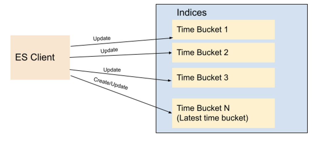
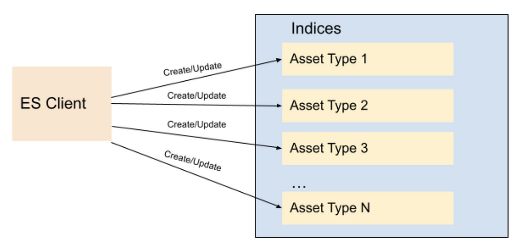
Most applications in content and studio engineering at Netflix deal with assets; such as videos, images, text, etc. These applications are built on a microservices architecture, and the Asset Management Platform provides asset management to those dozens of services for various asset types. Each asset type is defined in a centralized schema registry service responsible for storing asset type taxonomies and relationships. Therefore, it initially seemed natural to create a different index for each asset type. When creating index mappings in Elasticsearch, one has to define the data type for each field. Since different asset types could potentially have fields with the same name but with different data types; having a separate index for each type would prevent such type collisions. Therefore we created around a dozen indices per asset type with fields mapping based on the asset type schema. As we onboarded new applications to our platform, we kept creating new indices for the new asset types. We have a schema management microservice which is used to store the taxonomy of each asset type; and this programmatically created new indices whenever new asset types were created in this service. All the assets of a specific type use the specific index defined for that asset type to create or update the asset document.

Fig 1. Indices based on Asset Types

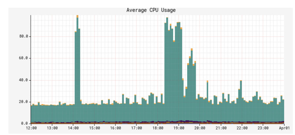
As Netflix is now producing significantly more originals than it used to when we started this project a few years ago, not only did the number of assets grow dramatically but also the number of asset types grew from dozens to several thousands. Hence the number of Elasticsearch indices (per asset type) as well as asset document indexing or searching RPS (requests per second) grew over time. Although this indexing strategy worked smoothly for a while, interesting challenges started coming up and we started to notice performance issues over time. We started to observe CPU spikes, long running queries, instances going yellow/red in status.

Usually the first thing to try is to scale up the Elasticsearch cluster horizontally by increasing the number of nodes or vertically by upgrading instance types. We tried both, and in many cases it helps, but sometimes it is a short term fix and the performance problems come back after a while; and it did for us. You know it is time to dig deeper to understand the root cause of it.

It was time to take a step back and reevaluate our ES data indexing and sharding strategy. Each index was assigned a fixed number of 6 shards and 2 replicas (defined in the template of the index). With the increase in the number of asset types, we ended up having approximately 900 indices (thus 16200 shards). Some of these indices had millions of documents, whereas many of them were very small with only thousands of documents. We found the root cause of the CPU spike was unbalanced shards size. Elasticsearch nodes storing those large shards became hot spots and queries hitting those instances were timing out or very slow due to busy threads.

We changed our indexing strategy and decided to create indices based on time buckets, rather than asset types. What this means is, assets created between t1 and t2 would go to the T1 bucket, assets created between t2 and t3 would go to the T2 bucket, and so on. So instead of persisting assets based on their asset types, we would use their ids (thus its creation time; because the asset id is a time based uuid generated at the asset creation) to determine which time bucket the document should be persisted to. Elasticsearch recommends each shard to be under 65GB (AWS recommends them to be under 50GB), so we could create time based indices where each index holds somewhere between 16–20GB of data, giving some buffer for data growth. Existing assets can be redistributed appropriately to these precreated shards, and new assets would always go to the current index. Once the size of the current index exceeds a certain threshold (16GB), we would create a new index for the next bucket (minute/hour/day) and start indexing assets to the new index created. We created an index template in Elasticsearch so that the new indices always use the same settings and mappings stored in the template.

We chose to index all versions of an asset in the the same bucket – the one that keeps the first version. Therefore, even though new assets can never be persisted to an old index (due to our time based id generation logic, they always go to the latest/current index); existing assets can be updated, causing additional documents for those new asset versions to be created in those older indices. Therefore we chose a lower threshold for the roll over so that older shards would still be well under 50GB even after those updates.

Fig 2. Indices based on Time Buckets

For searching purposes, we have a single read alias that points to all indices created. When performing a query, we always execute it on the alias. This ensures that no matter where documents are, all documents matching the query will be returned. For indexing/updating documents, though, we cannot use an alias, we use the exact index name to perform index operations.

To avoid the ES query for the list of indices for every indexing request, we keep the list of indices in a distributed cache. We refresh this cache whenever a new index is created for the next time bucket, so that new assets will be indexed appropriately. For every asset indexing request, we look at the cache to determine the corresponding time bucket index for the asset. The cache stores all time-based indices in a sorted order (for simplicity we named our indices based on their starting time in the format yyyyMMddHHmmss) so that we can easily determine exactly which index should be used for asset indexing based on the asset creation time. Without using the time bucket strategy, the same asset could have been indexed into multiple indices because Elasticsearch doc id is unique per index and not the cluster. Or we would have to perform two API calls, first to identify the specific index and then to perform the asset update/delete operation on that specific index.

It is still possible to exceed 50GB in those older indices if millions of updates occur within that time bucket index. To address this issue, we added an API that would split an old index into two programmatically. In order to split a given bucket T1 (which stores all assets between t1 and t2) into two, we choose a time t1.5 between t1 and t2, create a new bucket T1_5, and reindex all assets created between t1.5 and t2 from T1 into this new bucket. While the reindexing is happening, queries / reads are still answered by T1, so any new document created (via asset updates) would be dual-written into T1 and T1.5, provided that their timestamp falls between t1.5 and t2. Finally, once the reindexing is complete, we enable reads from T1_5, stop the dual write and delete reindexed documents from T1.

In fact, Elasticsearch provides an index rollover feature to handle the growing indicex problem https://www.elastic.co/guide/en/elasticsearch/reference/6.0/indices-rollover-index.html. With this feature, a new index is created when the current index size hits a threshold, and through a write alias, the index calls will point to the new index created. That means, all future index calls would go to the new index created. However, this would create a problem for our update flow use case, because we would have to query multiple indices to determine which index contains a particular document so that we can update it appropriately. Because the calls to Elasticsearch may not be sequential, meaning, an asset a1 created at T1 can be indexed after another asset a2 created at T2 where T2>T1, the older asset a1 can end up in the newer index while the newer asset a2 is persisted in the old index. In our current implementation, however, by simply looking at the asset id (and asset creation time), we can easily find out which index to go to and it is always deterministic.

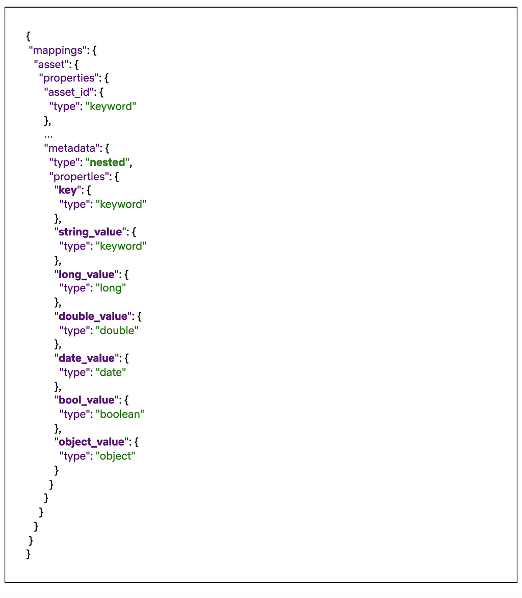
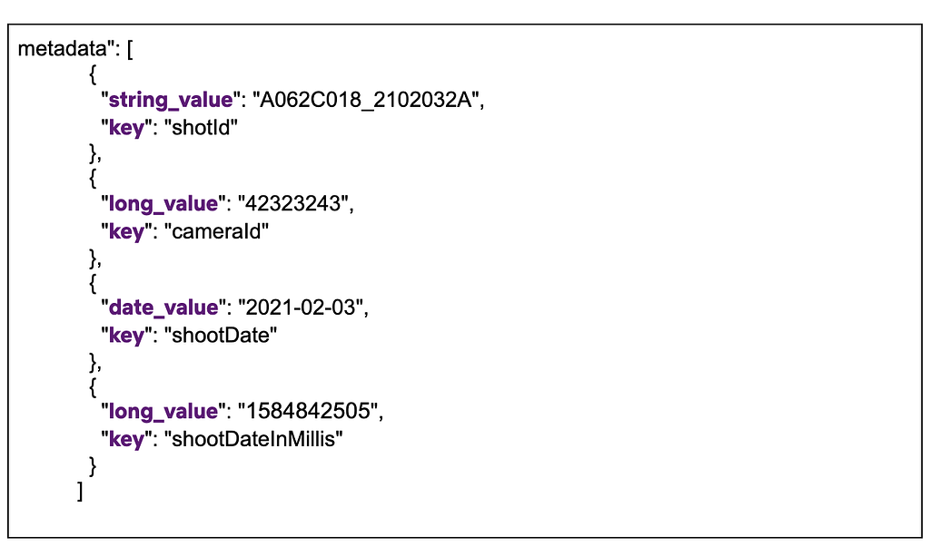
One thing to mention is, Elasticsearch has a default limit of 1000 fields per index. If we index all types to a single index, wouldn’t we easily exceed this number? And what about the data type collisions we mentioned above? Having a single index for all data types could potentially cause collisions when two asset types define different data types for the same field. We also changed our mapping strategy to overcome these issues. Instead of creating a separate Elasticsearch field for each metadata field defined in an asset type, we created a single nested type with a mandatory field called `key`, which represents the name of the field on the asset type, and a handful of data-type specific fields, such as: `string_value`, `long_value`, `date_value`, etc. We would populate the corresponding data-type specific field based on the actual data type of the value. Below you can see a part of the index mapping defined in our template, and an example from a document (asset) which has four metadata fields:

Fig 3. Snippet of the index mapping
Fig 4. Snippet of nested metadata field on a stored document

As you see above, all asset properties go under the same nested field `metadata` with a mandatory `key` field, and the corresponding data-type specific field. This ensures that no matter how many asset types or properties are indexed, we would always have a fixed number of fields defined in the mapping. When searching for these fields, instead of querying for a single value (cameraId == 42323243), we perform a nested query where we query for both key and the value (key == cameraId AND long_value == 42323243). For more information on nested queries, please refer to this link.

Fig 5. Search/Indexing RPS

After these changes, the indices we created are now balanced in terms of data size. CPU utilization is down from an average of 70% to 10%. In addition, we are able to reduce the refresh interval time on these indices from our earlier setting 30 seconds to 1 sec in order to support use cases like read after write, which enables users to search and get a document after a second it was created

Fig 6. CPU Spike with Old indexing strategy
Fig 7. CPU Usage with New indexing strategy

We had to do a one time migration of the existing documents to the new indices. Thankfully we already have a framework in place that can query all assets from Cassandra and index them in Elasticsearch. Since doing full table scans in Cassandra is not generally recommended on large tables (due to potential timeouts), our cassandra schema contains several reverse indices that help us query all data efficiently. We also utilize Kafka to process these assets asynchronously without impacting our real time traffic. This infrastructure is used not only to index assets to Elasticsearch, but also to perform administrative operations on all or some assets, such as bulk updating assets, scanning / fixing problems on them, etc. Since we only focused on Elasticsearch indexing in this blog, we are planning to create another blog to talk about this infrastructure later.


Elasticsearch Indexing Strategy in Asset Management Platform (AMP) was originally published in Netflix TechBlog on Medium, where people are continuing the conversation by highlighting and responding to this story.

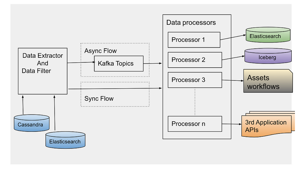
Data Reprocessing Pipeline in Asset Management Platform @Netflix

Post Syndicated from Netflix Technology Blog original https://netflixtechblog.com/data-reprocessing-pipeline-in-asset-management-platform-netflix-46fe225c35c9

By Meenakshi Jindal

Overview

At Netflix, we built the asset management platform (AMP) as a centralized service to organize, store and discover the digital media assets created during the movie production. Studio applications use this service to store their media assets, which then goes through an asset cycle of schema validation, versioning, access control, sharing, triggering configured workflows like inspection, proxy generation etc. This platform has evolved from supporting studio applications to data science applications, machine-learning applications to discover the assets metadata, and build various data facts.

During this evolution, quite often we receive requests to update the existing assets metadata or add new metadata for the new features added. This pattern grows over time when we need to access and update the existing assets metadata. Hence we built the data pipeline that can be used to extract the existing assets metadata and process it specifically to each new use case. This framework allowed us to evolve and adapt the application to any unpredictable inevitable changes requested by our platform clients without any downtime. Production assets operations are performed in parallel with older data reprocessing without any service downtime. Some of the common supported data reprocessing use cases are listed below.

Production Use Cases

  • Real-Time APIs (backed by the Cassandra database) for asset metadata access don’t fit analytics use cases by data science or machine learning teams. We build the data pipeline to persist the assets data in the iceberg in parallel with cassandra and elasticsearch DB. But to build the data facts, we need the complete data set in the iceberg and not just the new. Hence the existing assets data was read and copied to the iceberg tables without any production downtime.
  • Asset versioning scheme is evolved to support the major and minor version of assets metadata and relations update. This feature support required a significant update in the data table design (which includes new tables and updating existing table columns). Existing data got updated to be backward compatible without impacting the existing running production traffic.
  • Elasticsearch version upgrade which includes backward incompatible changes, so all the assets data is read from the primary source of truth and reindexed again in the new indices.
  • Data Sharding strategy in elasticsearch is updated to provide low search latency (as described in blog post)
  • Design of new Cassandra reverse indices to support different sets of queries.
  • Automated workflows are configured for media assets (like inspection) and these workflows are required to be triggered for old existing assets too.
  • Assets Schema got evolved that required reindexing all assets data again in ElasticSearch to support search/stats queries on new fields.
  • Bulk deletion of assets related to titles for which license is expired.
  • Updating or Adding metadata to existing assets because of some regressions in client application/within service itself.

Data Reprocessing Pipeline Flow

Figure 1. Data Reprocessing Pipeline Flow

Data Extractor

Cassandra is the primary data store of the asset management service. With SQL datastore, it was easy to access the existing data with pagination regardless of the data size. But there is no such concept of pagination with No-SQL datastores like Cassandra. Some features are provided by Cassandra (with newer versions) to support pagination like pagingstate, COPY, but each one of them has some limitations. To avoid dependency on data store limitations, we designed our data tables such that the data can be read with pagination in a performant way.

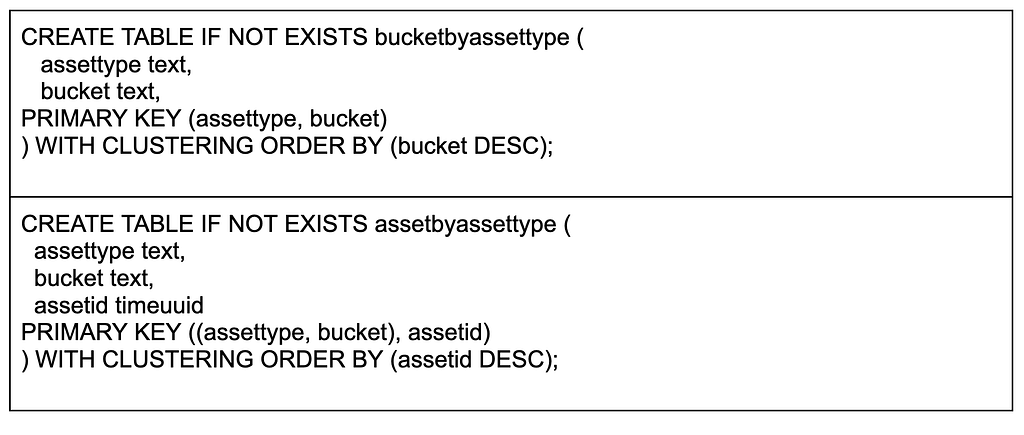
Mainly we read the assets data either by asset schema types or time bucket based on asset creation time. Data sharding completely based on the asset type may have created the wide rows considering some types like VIDEO may have many more assets compared to others like TEXT. Hence, we used the asset types and time buckets based on asset creation date for data sharding across the Cassandra nodes. Following is the example of tables primary and clustering keys defined:

Figure 2. Cassandra Table Design

Based on the asset type, first time buckets are fetched which depends on the creation time of assets. Then using the time buckets and asset types, a list of assets ids in those buckets are fetched. Asset Id is defined as a cassandra Timeuuid data type. We use Timeuuids for AssetId because it can be sorted and then used to support pagination. Any sortable Id can be used as the table primary key to support the pagination. Based on the page size e.g. N, first N rows are fetched from the table. Next page is fetched from the table with limit N and asset id < last asset id fetched.

Figure 3. Cassandra Data Fetch Query

Data layers can be designed based on different business specific entities which can be used to read the data by those buckets. But the primary id of the table should be sortable to support the pagination.

Sometimes we have to reprocess a specific set of assets only based on some field in the payload. We can use Cassandra to read assets based on time or an asset type and then further filter from those assets which satisfy the user’s criteria. Instead we use Elasticsearch to search those assets which are more performant.

After reading the asset ids using one of the ways, an event is created per asset id to be processed synchronously or asynchronously based on the use case. For asynchronous processing, events are sent to Apache Kafka topics to be processed.

Data Processor

Data processor is designed to process the data differently based on the use case. Hence, different processors are defined which can be extended based on the evolving requirements. Data can be processed synchronously or asynchronously.

Synchronous Flow: Depending on the event type, the specific processor can be directly invoked on the filtered data. Generally, this flow is used for small datasets.

Asynchronous Flow: Data processor consumes the data events sent by the data extractor. Apache Kafka topic is configured as a message broker. Depending on the use case, we have to control the number of events processed in a time unit e.g. to reindex all the data in elasticsearch because of template change, it is preferred to re-index the data at certain RPS to avoid any impact on the running production workflow. Async processing has the benefit to control the flow of event processing with Kafka consumers count or with controlling thread pool size on each consumer. Event processing can also be stopped at any time by disabling the consumers in case production flow gets any impact with this parallel data processing. For fast processing of the events, we use different settings of Kafka consumer and Java executor thread pool. We poll records in bulk from Kafka topics, and process them asynchronously with multiple threads. Depending on the processor type, events can be processed at high scale with right settings of consumer poll size and thread pool.

Each of these use cases mentioned above looks different, but they all need the same reprocessing flow to extract the old data to be processed. Many applications design data pipelines for the processing of the new data; but setting up such a data processing pipeline for the existing data supports handling the new features by just implementing a new processor. This pipeline can be thoughtfully triggered anytime with the data filters and data processor type (which defines the actual action to be performed).

Error Handling

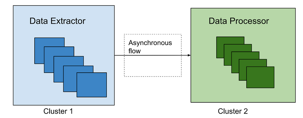
Errors are part of software development. But with this framework, it has to be designed more carefully as bulk data reprocessing will be done in parallel with the production traffic. We have set up the different clusters of data extractor and processor from the main Production cluster to process the older assets data to avoid any impact of the assets operations live in production. Such clusters may have different configurations of thread pools to read and write data from database, logging levels and connection configuration with external dependencies.

Figure 4: Processing clusters

Data processors are designed to continue processing the events even in case of some errors for eg. There are some unexpected payloads in old data. In case of any error in the processing of an event, Kafka consumers acknowledge that event is processed and send those events to a different queue after some retries. Otherwise Kafka consumers will continue trying to process the same message again and block the processing of other events in the topic. We reprocess data in the dead letter queue after fixing the root cause of the issue. We collect the failure metrics to be checked and fixed later. We have set up the alerts and continuously monitor the production traffic which can be impacted because of the bulk old data reprocessing. In case any impact is noticed, we should be able to slow down or stop the data reprocessing at any time. With different data processor clusters, this can be easily done by reducing the number of instances processing the events or reducing the cluster to 0 instances in case we need a complete halt.

Best Practices

  • Depending on existing data size and use case, processing may impact the production flow. So identify the optimal event processing limits and accordingly configure the consumer threads.
  • If the data processor is calling any external services, check the processing limits of those services because bulk data processing may create unexpected traffic to those services and cause scalability/availability issues.
  • Backend processing may take time from seconds to minutes. Update the Kafka consumer timeout settings accordingly otherwise different consumer may try to process the same event again after processing timeout.
  • Verify the data processor module with a small data set first, before trigger processing of the complete data set.
  • Collect the success and error processing metrics because sometimes old data may have some edge cases not handled correctly in the processors. We are using the Netflix Atlas framework to collect and monitor such metrics.

Acknowledgements

Burak Bacioglu and other members of the Asset Management platform team have contributed in the design and development of this data reprocessing pipeline.


Data Reprocessing Pipeline in Asset Management Platform @Netflix was originally published in Netflix TechBlog on Medium, where people are continuing the conversation by highlighting and responding to this story.

Cloudflare’s network expansion in Indonesia

Post Syndicated from Joanne Liew original https://blog.cloudflare.com/indonesia/

Cloudflare's network expansion in Indonesia

Cloudflare's network expansion in Indonesia

As home to over 200 million Internet users and the fourth-largest population in the world, Indonesians depend on fast and reliable Internet, but this has always been a challenging part of the world for Internet infrastructure. This has real world implications on performance and reliability (IP transit is on average 6x more expensive than our major South East Asian interconnection markets). That said, first we wanted to share what makes things challenging in Indonesia; geography, infrastructure, and market dynamics.

Geography: The Internet backbone for many countries is almost entirely delivered by terrestrial fiber optic cables, where connectivity is more affordable and easier to build when the land mass is contiguous and there is a concentrated population distribution. However, Indonesia is a collection of over 18,000 islands, spanning three time zones, and approximately 3,200 miles (5,100 km) east to west. By comparison, the United States is 2,800 miles (4,500 km) east to west. While parts of Indonesia are geographically close to Singapore (the regional Internet hub with over 60% of the region’s data centers) given how large Indonesia is, much of it is far away.

Infrastructure: Indonesia is a large country and to connect it to the rest of the Internet it currently relies on submarine fiber optic cables. There are a total of 22 separate submarine cables connecting Indonesia to Singapore, Malaysia, Australia and onward. Many of the cable systems cross the Strait of Malacca, a narrow stretch of water, between the Malay Peninsula (Peninsular Malaysia) and the Indonesian island of Sumatra to the southwest, connecting the Indian and Pacific Oceans. This makes reliability challenging as a result of human activities, such as ships dropping their anchors, fishing trawlers, and dredging as it is one of the world’s top five busiest shipping lanes. Additionally, Indonesia is geographically located in a very active seismic zone and is very earthquake prone.

There are a number of new submarine cable systems that have come online and four significant builds planned (Apricot, ACC-1, Echo and Nui) that will improve both available capacity and cost economics in the market. Right now the cost is still significantly higher than comparable distances. For example Jakarta to Singapore is approximately 60 times more expensive than a service the same distance would be in the continental US or Europe for a 100Gbps wavelength service. Staying in Asia, a similar distance from Hong Kong to Taiwan costs around 1/6th that of Jakarta to Singapore.

Cloudflare's network expansion in Indonesia

Cloudflare's network expansion in Indonesia
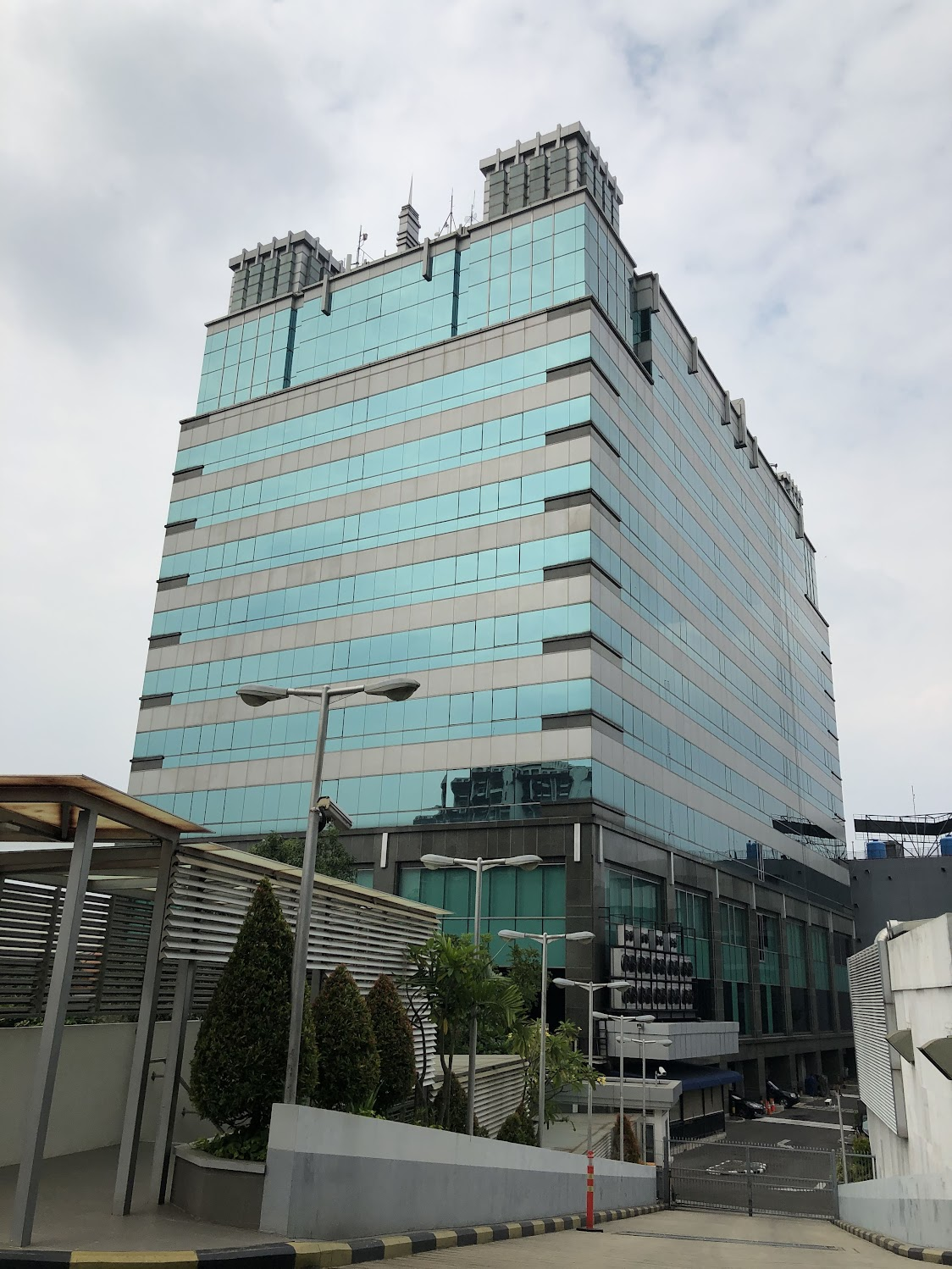
Cyber 1 and Cyber 3 (NTT NexCenter) Data Center Buildings in Jakarta, 2019 (Photo Credit: Tom Paseka).

Cloudflare's network expansion in Indonesia
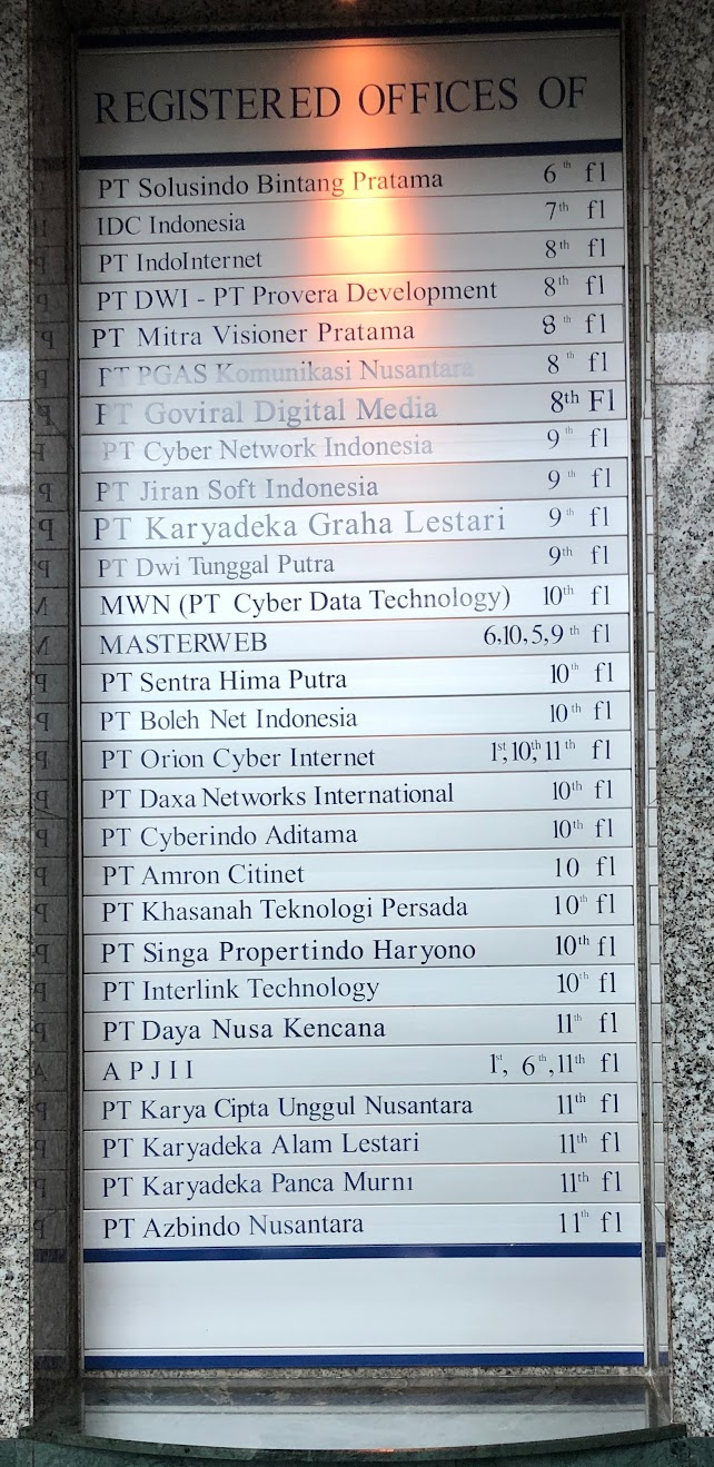
Picture of Cyber 1 Lobby Directory

While areas like Batam are becoming increasingly popular for data center builds due to its proximity to Singapore, Jakarta is still the most developed and mature market. It has the largest and best interconnected data centers in the country, including the two pictured.

Cloudflare is deployed in the facility on the right (NTT NexCenter), however most ISPs are inside the building on the left (Cyber 1). The two buildings are approximately 30-50 meters apart, yet it’s surprisingly difficult to be able to connect between them. One of the reasons why is market fragmentation and how many options are available. In the adjacent picture of the Cyber 1 building lobby directory many of the listings are unique data centers each with different policies and access conditions.

In the past, we’ve talked about the Cost of Bandwidth around the world (and updated here), but we’ve never talked about Indonesia specifically. Using the same methodology as we’ve used in the past, Indonesia’s cost is 43x times more expensive than North America or Europe, or even multiples more expensive than other countries in Asia.

Market dynamics: While Indonesia has good and functioning Internet Exchanges, there are a few ISPs who dominate the market. The three largest ISPs in the country (Telkom Indonesia, Indosat Ooredoo Hutchison and XL Axiata) collectively control 80% of the market, while Telkom Indonesia alone has a market share of around 60% by revenue.

This results in Telkom Indonesia having a heavily dominant market share position to leverage resulting in refusal to peer, or exchange Internet traffic in Indonesia without expensive payments, or instead, preferring to connect to other networks outside of Indonesia, introducing latency and diminished performance.

Despite all of these challenges, our network has come a long way since our initial deployment to Jakarta in 2019.

We’ve established:

  • A carrier neutral local point of presence at NTT Indonesia Nexcenter Data Center, one of the major interconnection hubs in Jakarta
  • An edge partnership point of presence in Yogyakarta with CitranetIX
  • Direct interconnections in country with two of the top three networks.
  • Peering across three of the larger local internet exchanges, Indonesia Internet Exchange, Jakarta Internet Exchange and Biznet Internet Exchange
  • Dedicated 100G wavelength transport back to Singapore

All of this results in a more performant and reliable network for our local customers.

We wanted to see how our network is performing since deployment. We mentioned during Speed Week in 2021 how we benchmark against different networks, and sharing some of those benchmarks here.

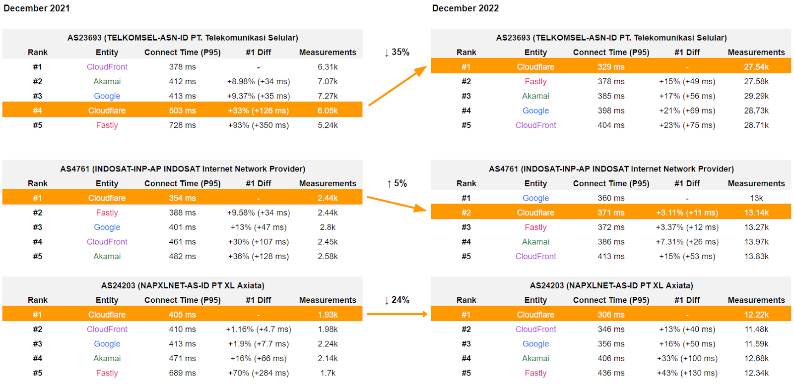
At the end of December 2021, Cloudflare was only faster in a few networks, as compared to other providers in Indonesia.

Cloudflare's network expansion in Indonesia

Fast forward twelve months to December 2022, Cloudflare is significantly faster in even more networks.

Cloudflare's network expansion in Indonesia

The TCP protocol is a connection-oriented protocol, which means that a connection is established and maintained until the application programs at each end have finished exchanging messages. The Connect Time summarizes how fast a session can be set up between a client and a server over a network. TTLB (or time to last byte) is the time taken to send the entire response to the web browser. It’s a good measure of how long a complete download takes. Check out our recent blog on Benchmarking Edge Network Performance for more information on how we measure the performance of our network and benchmark ourselves against industry players.

On closer inspection against the three major ISPs specifically, we’re the top provider for two out of the three networks. Cloudflare’s performance has improved year-on-year (16% reduction) and continues to lead (comparative to the other networks) meaning faster and more responsive services for our customers.

Cloudflare's network expansion in Indonesia

Helping build a better Internet for Indonesia doesn’t stop here and there is always more work to be done! We want to be the number one network everywhere and won’t rest until we are. We are continuing to connect to more networks locally, invest in direct submarine cable capacity, as well as further deployments into new data center buildings, Internet Exchanges and new cities too!

Are you operating a network and not yet peering with Cloudflare? Log-in to our Peering Portal or find out more information here for ways to set up peering, or request we deploy nodes into your network directly.

Metasploit Weekly Wrap-Up

Post Syndicated from Jack Heysel original https://blog.rapid7.com/2023/03/10/metasploit-weekly-wrap-up-196/

Wowza, a new credential gatherer and login scanner!

Metasploit Weekly Wrap-Up

This week Metasploit Framework gained a credential gatherer for Wowza Streaming Engine Manager. Credentials for this application are stored in a file named admin.password in a known location and the file is readable by default by BUILTIN\Users on Windows and is world readable on Linux.. The module was written by community contributor bcoles who also wrote a login scanner for Wowza this week. The login scanner can be used to validate the credentials found by the gatherer. The two modules complement each other quite nicely.

New module content (3)

Wowza Streaming Engine Manager Login Utility

Author: bcoles
Type: Auxiliary
Pull request: #17733 contributed by bcoles

Description: This adds a login scanner module to brute force credentials of Wowza Streaming Engine Manager.

SugarCRM unauthenticated Remote Code Execution (RCE)

Authors: Sw33t.0day and h00die-gr3y
Type: Exploit
Pull request: #17507 contributed by h00die-gr3y
AttackerKB reference: CVE-2023-22952

Description: A module has been added which exploits CVE-2023-22952, a RCE vulnerability in SugarCRM 11.0 Enterprise, Professional, Sell, Serve, and Ultimate versions prior to 11.0.5 and SugarCRM 12.0 Enterprise, Sell, and Serve versions prior to 12.0.2. Successful exploitation as an unauthenticated attacker will result in remote code execution as the user running the web services, which is typically www-data.

Gather Wowza Streaming Engine Credentials

Author: bcoles
Type: Post
Pull request: #17737 contributed by bcoles

Description: This adds a post module that collects Wowza Streaming Engine user credentials from the admin.password local configuration file. This file is world-readable by default on Linux and readable by BUILTIN\Users on Windows.

Enhancements and features (9)

  • #17675 from adfoster-r7 – Updates the admin/kerberos/forge_ticket to support a new extra_sids option which can be useful for including cross-domain SIDs for forging external Kerberos trust tickets as part of cross-trust domain escalation. The admin/kerberos/inspect_ticket has also been updated to support viewing these extra SID values.
  • #17686 from zeroSteiner – This adds 3 additional methods to the existing PetitPotam module to make it work even if the patch for CVE-2021-36942 has been installed. Note that it won’t work after the December 2021 patch.
  • #17715 from zeroSteiner – The Metasploit Payload gem has been bumped to 2.0.115, bringing in support for the arp command to Python Meterpreter on Linux, and adding support for displaying IPv6 routing tables using the route command on Windows.
  • #17727 from rohitkumarankam – Two new options have been added to the login scanner library: max_consecutive_error_count and max_error_count. These options allow users to set the maximum number of errors that are allowed to occur when connecting as well as the maximum number of consecutive errors that are allowed when connecting before the login scanner will give up on a target.
  • #17744 from adfoster-r7 – The code for msfconsole has been updated so that performance profiling can also take into account the time it takes to load msfenv and console related libraries, thereby allowing for more accurate performance profiling.
  • #17745 from gwillcox-r7 – This updates the metasploit-payloads gem to pull in changes to the Python Meterpreter on Windows to add the route add and route delete commands as well as the ability to get process information such as process names and paths.
  • #17746 from todb-r7 – The data/wordlists/password.lst password list has been updated to include the master password that LastPass suggests as an example when a user goes to create a new master password, r50$K28vaIFiYxaY, into the password list, as well as to fix some encoding issues.
  • #17749 from adfoster-r7 – Updates the auxiliary/admin/kerberos/keytab.rb module to additionally export any NTHASHES, which can be useful for decrypting Kerberos network traffic in Wireshark.
  • #17756 from adfoster-r7 – Updates secrets dump to generate the Kerberos RC4 key for the machine account.

Bugs fixed (8)

  • #17673 from bcoles – lib/msf/core/payload/apk.rb has been updated so that by default it only decompiles the main classes instead of all classes, fixing some issues whereby decompiling all classes would prevent creation of a backdoored APK. This also bumps up the minimum apktool version to 2.4.1 and makes it so that versions prior to 2.7.0 of apktool will throw a warning about being potentially out of date.
  • #17716 from zeroSteiner – A bug has been fixed whereby the reverse port forward information message was displayed incorrectly, and the same information was shown on both the local and remote parts of the message.
  • #17721 from zeroSteiner – This fixes an issue where payloads that were adapted failed when stage encoding was enabled because the stage encoding was based on the stager arch and platform values. These values were always the same until we introduced adapted payloads, which can vary.
  • #17723 from jvoisin – A bug has been fixed in the modules/encoders/php/base64.rb encoder whereby strings were being passed as literal strings without being properly quoted, which could result in errors on newer versions of PHP.
  • #17726 from zeroSteiner – The Metasploit Payloads gem has been updated bringing in initial support for attaching to processes on Python Meterpreter shells on Windows, a bug fix for the route command on newer versions of Windows on Windows Meterpreter, and a fix so that both C Meterpreter and Python Meterpreter sessions will attempt to enable the same set of permissions when running getprivs.
  • #17729 from bcoles – Fixes an edge case crash when running Ruby 3.2
  • #17738 from adfoster-r7 – Fix Ruby 3.2 crash when running certain tools
  • #17758 from zeroSteiner – The metasploit-payloads gem has been bumped to fix a token handle leak that was causing Python Meterpreters to leave dangling handles after using getprivs, fix a error in packet_transmit_http whereby error codes were not appropriately returned, and update the arp command to properly return the interface name instead of the index for the interface column.

Documentation added (3)

  • #17684 from adfoster-r7 – This PR adds the RBCD exploitation documentation to the docs site.
  • #17688 from adfoster-r7 – This PR fixes several broken wiki links, as well as adding validation to users users don’t use the wrong syntax when making docs changes.
  • #17743 from adfoster-r7 – A new page has been added to explain the METASPLOIT_CPU_PROFILE and METASPLOIT_MEMORY_PROFILE options and to explain how to profile msfconsole‘s and msfvenom‘s performance on systems.

You can always find more documentation on our docsite at docs.metasploit.com.

Get it

As always, you can update to the latest Metasploit Framework with msfupdate
and you can get more details on the changes since the last blog post from
GitHub:

If you are a git user, you can clone the Metasploit Framework repo (master branch) for the latest.
To install fresh without using git, you can use the open-source-only Nightly Installers or the
binary installers (which also include the commercial edition).

Build a serverless transactional data lake with Apache Iceberg, Amazon EMR Serverless, and Amazon Athena

Post Syndicated from Houssem Chihoub original https://aws.amazon.com/blogs/big-data/build-a-serverless-transactional-data-lake-with-apache-iceberg-amazon-emr-serverless-and-amazon-athena/

Since the deluge of big data over a decade ago, many organizations have learned to build applications to process and analyze petabytes of data. Data lakes have served as a central repository to store structured and unstructured data at any scale and in various formats. However, as data processing at scale solutions grow, organizations need to build more and more features on top of their data lakes. One important feature is to run different workloads such as business intelligence (BI), Machine Learning (ML), Data Science and data exploration, and Change Data Capture (CDC) of transactional data, without having to maintain multiple copies of data. Additionally, the task of maintaining and managing files in the data lake can be tedious and sometimes complex.

Table formats like Apache Iceberg provide solutions to these issues. They enable transactions on top of data lakes and can simplify data storage, management, ingestion, and processing. These transactional data lakes combine features from both the data lake and the data warehouse. You can simplify your data strategy by running multiple workloads and applications on the same data in the same location. However, using these formats requires building, maintaining, and scaling infrastructure and integration connectors that can be time-consuming, challenging, and costly.

In this post, we show how you can build a serverless transactional data lake with Apache Iceberg on Amazon Simple Storage Service (Amazon S3) using Amazon EMR Serverless and Amazon Athena. We provide an example for data ingestion and querying using an ecommerce sales data lake.

Apache Iceberg overview

Iceberg is an open-source table format that brings the power of SQL tables to big data files. It enables ACID transactions on tables, allowing for concurrent data ingestion, updates, and queries, all while using familiar SQL. Iceberg employs internal metadata management that keeps track of data and empowers a set of rich features at scale. It allows you to time travel and roll back to old versions of committed data transactions, control the table’s schema evolution, easily compact data, and employ hidden partitioning for fast queries.

Iceberg manages files on behalf of the user and unlocks use cases such as:

  • Concurrent data ingestion and querying, including streaming and CDC
  • BI and reporting with expressive simple SQL
  • Empowering ML feature stores and training sets
  • Compliance and regulations workloads, such as GDPR find and forget
  • Reinstating late-arriving data, which is dimensions data arriving later than the fact data. For example, the reason for a flight delay may arrive well after the fact that the fligh is delayed.
  • Tracking data changes and rollback

Build your transactional data lake on AWS

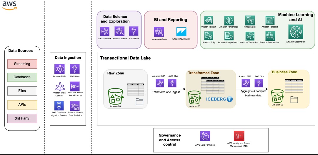
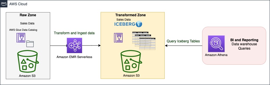
You can build your modern data architecture with a scalable data lake that integrates seamlessly with an Amazon Redshift powered cloud warehouse. Moreover, many customers are looking for an architecture where they can combine the benefits of a data lake and a data warehouse in the same storage location. In the following figure, we show a comprehensive architecture that uses the modern data architecture strategy on AWS to build a fully featured transactional data lake. AWS provides flexibility and a wide breadth of features to ingest data, build AI and ML applications, and run analytics workloads without having to focus on the undifferentiated heavy lifting.

Data can be organized into three different zones, as shown in the following figure. The first zone is the raw zone, where data can be captured from the source as is. The transformed zone is an enterprise-wide zone to host cleaned and transformed data in order to serve multiple teams and use cases. Iceberg provides a table format on top of Amazon S3 in this zone to provide ACID transactions, but also to allow seamless file management and provide time travel and rollback capabilities. The business zone stores data specific to business cases and applications aggregated and computed from data in the transformed zone.

One important aspect to a successful data strategy for any organization is data governance. On AWS, you can implement a thorough governance strategy with fine-grained access control to the data lake with AWS Lake Formation.

Serverless architecture overview

In this section, we show you how to ingest and query data in your transactional data lake in a few steps. EMR Serverless is a serverless option that makes it easy for data analysts and engineers to run Spark-based analytics without configuring, managing, and scaling clusters or servers. You can run your Spark applications without having to plan capacity or provision infrastructure, while paying only for your usage. EMR Serverless supports Iceberg natively to create tables and query, merge, and insert data with Spark. In the following architecture diagram, Spark transformation jobs can load data from the raw zone or source, apply the cleaning and transformation logic, and ingest data in the transformed zone on Iceberg tables. Spark code can run instantaneously on an EMR Serverless application, which we demonstrate later in this post.

The Iceberg table is synced with the AWS Glue Data Catalog. The Data Catalog provides a central location to govern and keep track of the schema and metadata. With Iceberg, ingestion, update, and querying processes can benefit from atomicity, snapshot isolation, and managing concurrency to keep a consistent view of data.

Athena is a serverless, interactive analytics service built on open-source frameworks, supporting open-table and file formats. Athena provides a simplified, flexible way to analyze petabytes of data where it lives. To serve BI and reporting analysis, it allows you to build and run queries on Iceberg tables natively and integrates with a variety of BI tools.

Sales data model

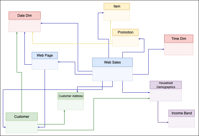
Star schema and its variants are very popular for modeling data in data warehouses. They implement one or more fact tables and dimension tables. The fact table stores the main transactional data from the business logic with foreign keys to dimensional tables. Dimension tables hold additional complementary data to enrich the fact table.

In this post, we take the example of sales data from the TPC-DS benchmark. We zoom in on a subset of the schema with the web_sales fact table, as shown in the following figure. It stores numeric values about sales cost, ship cost, tax, and net profit. Additionally, it has foreign keys to dimensional tables like date_dim, time_dim, customer, and item. These dimensional tables store records that give more details. For instance, you can show when a sale took place by which customer for which item.

Dimension-based models have been used extensively to build data warehouses. In the following sections, we show how to implement such a model on top of Iceberg, providing data warehousing features on top of your data lake, and run different workloads in the same location. We provide a complete example of building a serverless architecture with data ingestion using EMR Serverless and Athena using TPC-DS queries.

Prerequisites

For this walkthrough, you should have the following prerequisites:

  • An AWS account
  • Basic knowledge about data management and SQL

Deploy solution resources with AWS CloudFormation

We provide an AWS CloudFormation template to deploy the data lake stack with the following resources:

  • Two S3 buckets: one for scripts and query results, and one for the data lake storage
  • An Athena workgroup
  • An EMR Serverless application
  • An AWS Glue database and tables on external public S3 buckets of TPC-DS data
  • An AWS Glue database for the data lake
  • An AWS Identity and Access Management (IAM) role and polices

Complete the following steps to create your resources:

  1. Launch the CloudFormation stack:

Launch Button

This automatically launches AWS CloudFormation in your AWS account with the CloudFormation template. It prompts you to sign in as needed.

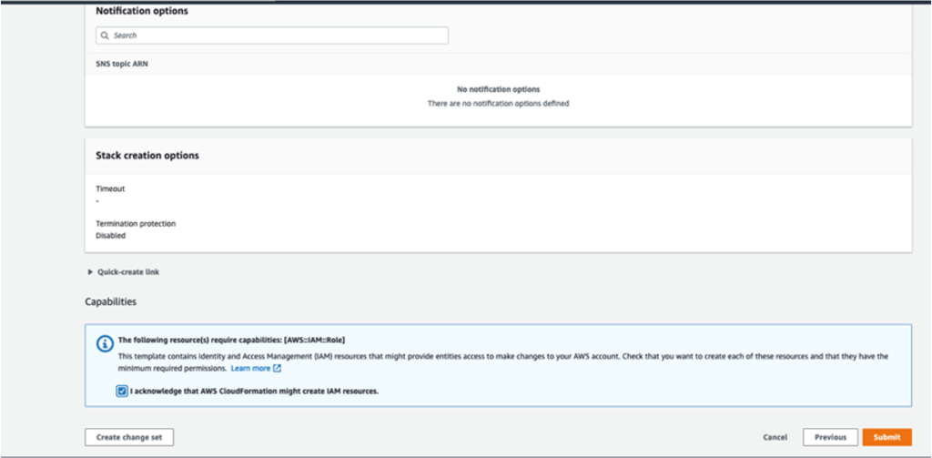
  1. Keep the template settings as is.
  2. Check the I acknowledge that AWS CloudFormation might create IAM resources box.
  3. Choose Submit

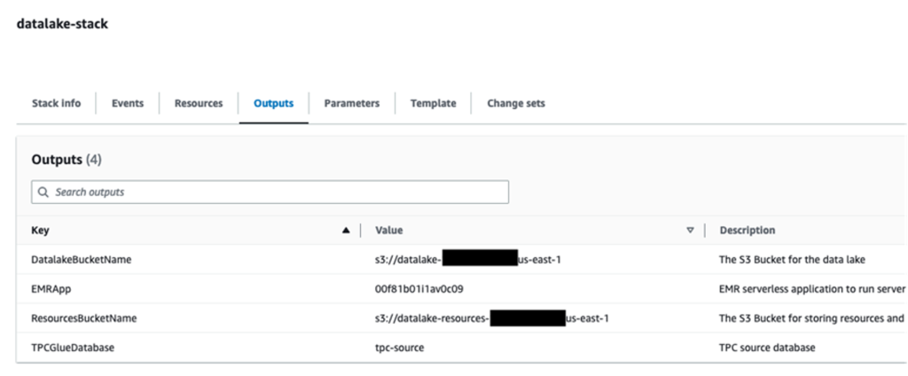
When the stack creation is complete, check the Outputs tab of the stack to verify the resources created.

Upload Spark scripts to Amazon S3

Complete the following steps to upload your Spark scripts:

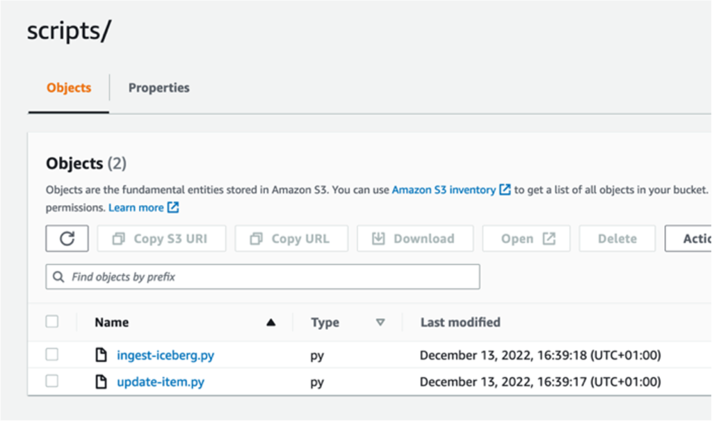
  1. Download the following scripts: ingest-iceberg.py and update-item.py.
  2. On the Amazon S3 console, go to the datalake-resources-<AccountID>-us-east-1 bucket you created earlier.
  3. Create a new folder named scripts.
  4. Upload the two PySpark scripts: ingest-iceberg.py and update-item.py.

Create Iceberg tables and ingest TPC-DS data

To create your Iceberg tables and ingest the data, complete the following steps:

  1. On the Amazon EMR console, choose EMR Serverless in the navigation pane.
  2. Choose Manage applications.
  3. Choose the application datalake-app.

  1. Choose Start application.

Once started, it will provision the pre-initialized capacity as configured at creation (one Spark driver and two Spark executors). The pre-initialized capacity are resources that will be provisioned when you start your application. They can be used instantly when you submit jobs. However, they incur charges even if they’re not used when the application is in a started state. By default, the application is set to stop when idle for 15 minutes.

Now that the EMR application has started, we can submit the Spark ingest job ingest-iceberg.py. The job creates the Iceberg tables and then loads data from the previously created AWS Glue Data Catalog tables on TPC-DS data in an external bucket.

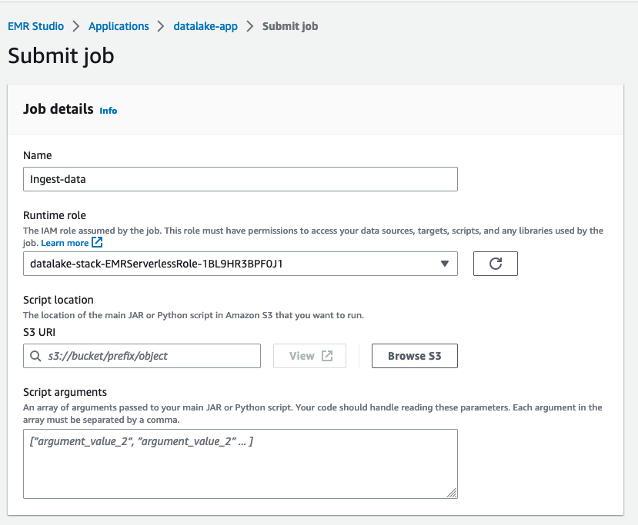
  1. Navigate to the datalake-app.
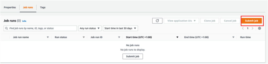
  2. On the Job runs tab, choose Submit job.

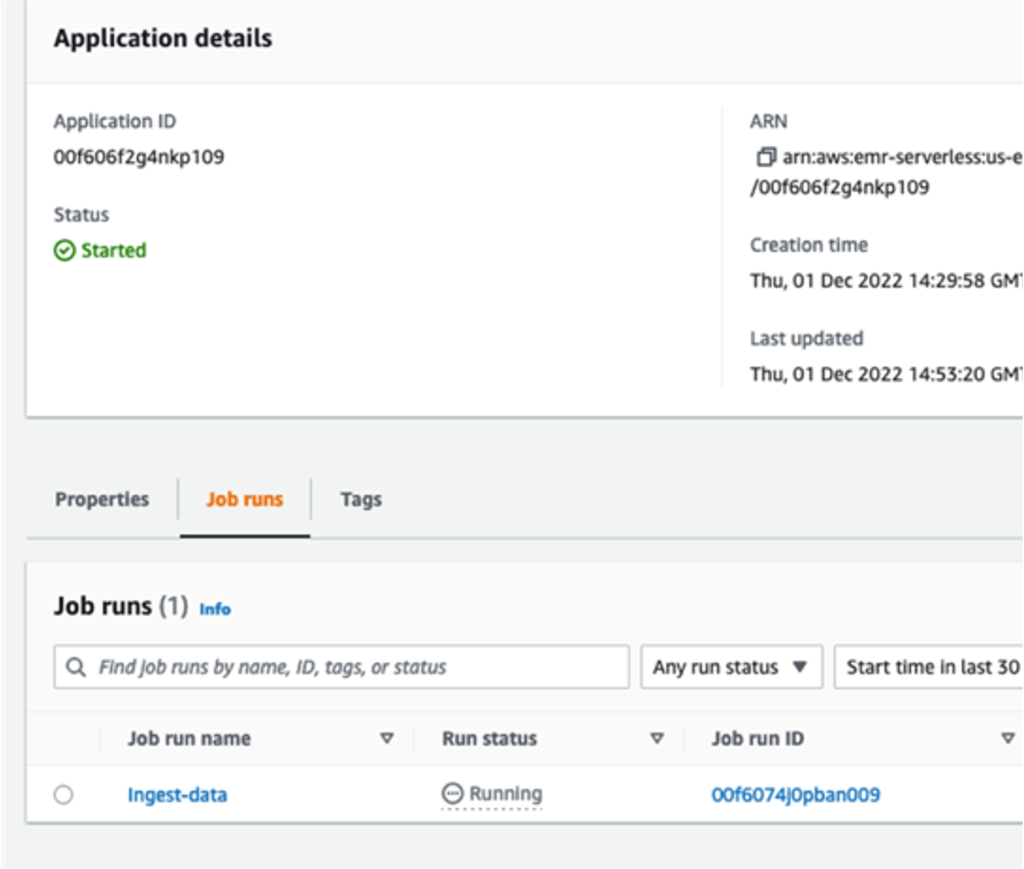
  1. For Name, enter ingest-data.
  2. For Runtime role, choose the IAM role created by the CloudFormation stack.
  3. For Script location, enter the S3 path for your resource bucket (datalake-resource-<####>-us-east-1>scripts>ingest-iceberg.py).

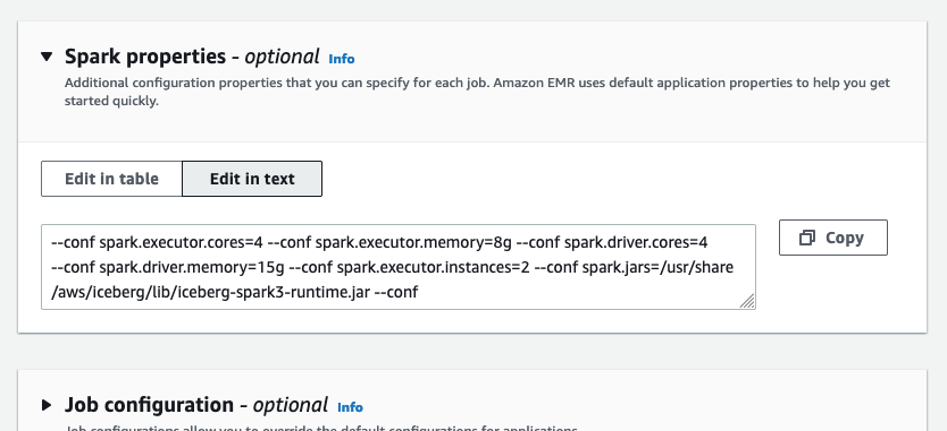
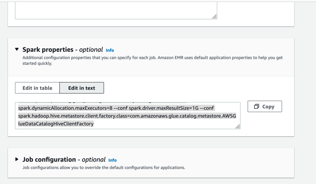
  1. Under Spark properties, choose Edit in text.
  2. Enter the following properties, replacing <BUCKET_NAME> with your data lake bucket name datalake-<####>-us-east-1 (not datalake-resources)
--conf spark.executor.cores=2 --conf spark.executor.memory=4g --conf spark.driver.cores=2 --conf spark.driver.memory=8g --conf spark.executor.instances=2 --conf spark.jars=/usr/share/aws/iceberg/lib/iceberg-spark3-runtime.jar --conf spark.sql.extensions=org.apache.iceberg.spark.extensions.IcebergSparkSessionExtensions --conf spark.sql.catalog.dev.warehouse=s3://<BUCKET_NAME>/warehouse --conf spark.sql.catalog.dev=org.apache.iceberg.spark.SparkCatalog --conf spark.sql.catalog.dev.catalog-impl=org.apache.iceberg.aws.glue.GlueCatalog --conf spark.sql.catalog.glue_catalog.lock-impl=org.apache.iceberg.aws.glue.DynamoLockManager --conf spark.sql.catalog.glue_catalog.lock.table=myIcebergLockTab --conf spark.dynamicAllocation.maxExecutors=8 --conf spark.driver.maxResultSize=1G --conf spark.hadoop.hive.metastore.client.factory.class=com.amazonaws.glue.catalog.metastore.AWSGlueDataCatalogHiveClientFactory

  1. Submit the job.

You can monitor the job progress.

Query Iceberg tables

In this section, we provide examples of data warehouse queries from TPC-DS on the Iceberg tables.

  1. On the Athena console, open the query editor.
  2. For Workgroup, switch to DatalakeWorkgroup.

  1. Choose Acknowledge.

The queries in DatalakeWorkgroup will run on Athena engine version 3.

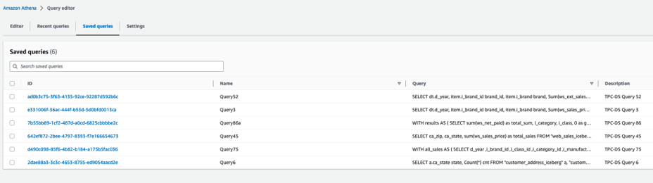
  1. On the Saved queries tab, choose a query to run on your Iceberg tables.

The following queries are listed:

  • Query3 – Report the total extended sales price per item brand of a specific manufacturer for all sales in a specific month of the year.
  • Query45 – Report the total web sales for customers in specific zip codes, cities, counties, or states, or specific items for a given year and quarter.
  • Query52 – Report the total of extended sales price for all items of a specific brand in a specific year and month.
  • Query6 – List all the states with at least 10 customers who during a given month bought items with the price tag at least 20% higher than the average price of items in the same category.
  • Query75 – For 2 consecutive years, track the sales of items by brand, class, and category.
  • Query86a – Roll up the web sales for a given year by category and class, and rank the sales among peers within the parent. For each group, compute the sum of sales and location with the hierarchy and rank within the group.

These queries are examples of queries used in decision-making and reporting in an organization. You can run them in the order you want. For this post, we start with Query3.

  1. Before you run the query, confirm that Database is set to datalake.

  1. Now you can run the query.

  1. Repeat these steps to run the other queries.

Update the item table

After running the queries, we prepare a batch of updates and inserts of records into the item table.

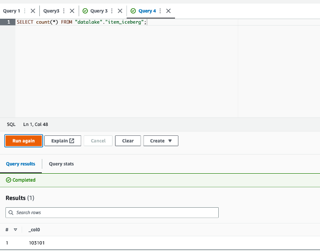
  1. First, run the following query to count the number of records in the item Iceberg table:
SELECT count(*) FROM "datalake"."item_iceberg";

This should return 102,000 records.

  1. Select item records with a price higher than $90:
SELECT count(*) FROM "datalake"."item_iceberg" WHERE i_current_price > 90.0;

This will return 1,112 records.

The update-item.py job takes these 1,112 records, modifies 11 records to change the name of the brand to Unknown, and changes the remaining 1,101 records’ i_item_id key to flag them as new records. As a result, a batch of 11 updates and 1,101 inserts are merged into the item_iceberg table.

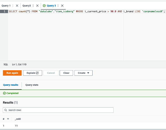
The 11 records to be updated are those with price higher than $90, and the brand name starts with corpnameless.

  1. Run the following query:
SELECT count(*) FROM "datalake"."item_iceberg" WHERE i_current_price > 90.0 AND i_brand LIKE 'corpnameless%';

The result is 11 records. The item_update.py job replaces the brand name with Unknown and merges the batch into the Iceberg table.

Now you can return to the EMR Serverless console and run the job on the EMR Serverless application.

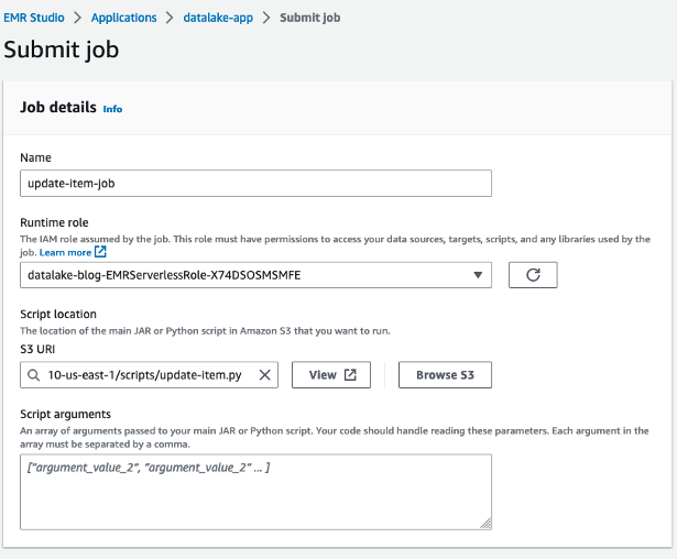
  1. On the application details page, choose Submit job.
  2. For Name, enter update-item-job.
  3. For Runtime role¸ use the same role that you used previously.
  4. For S3 URI, enter the update-item.py script location.

  1. Under Spark properties, choose Edit in text.
  2. Enter the following properties, replacing the <BUCKET-NAME> with your own datalake-<####>-us-east-1:
--conf spark.executor.cores=2 --conf spark.executor.memory=8g --conf spark.driver.cores=4 --conf spark.driver.memory=8g --conf spark.executor.instances=2 --conf spark.jars=/usr/share/aws/iceberg/lib/iceberg-spark3-runtime.jar --conf spark.sql.extensions=org.apache.iceberg.spark.extensions.IcebergSparkSessionExtensions --conf spark.sql.catalog.dev=org.apache.iceberg.spark.SparkCatalog --conf spark.sql.catalog.dev.catalog-impl=org.apache.iceberg.aws.glue.GlueCatalog --conf spark.sql.catalog.glue_catalog.lock-impl=org.apache.iceberg.aws.glue.DynamoLockManager --conf spark.sql.catalog.glue_catalog.lock.table=myIcebergLockTab --conf spark.dynamicAllocation.maxExecutors=4 --conf spark.driver.maxResultSize=1G --conf spark.sql.catalog.dev.warehouse=s3://<BUCKET-NAME>/warehouse --conf spark.hadoop.hive.metastore.client.factory.class=com.amazonaws.glue.catalog.metastore.AWSGlueDataCatalogHiveClientFactory

  1. Then submit the job.

  1. After the job finishes successfully, return to the Athena console and run the following query:
SELECT count(*) FROM "datalake"."item_iceberg";

The returned result is 103,101 = 102,000 + (1,112 – 11). The batch was merged successfully.

Time travel

To run a time travel query, complete the following steps:

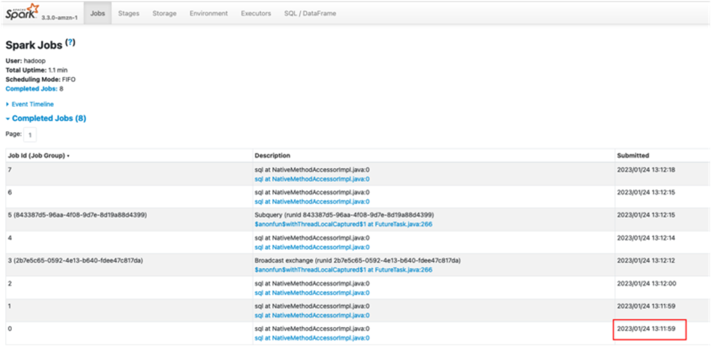
  1. Get the timestamp of the job run via the application details page on the EMR Serverless console, or the Spark UI on the History Server, as shown in the following screenshot.

This time could be just minutes before you ran the update Spark job.

  1. Convert the timestamp from the format YYYY/MM/DD hh:mm:ss to YYYY-MM-DDThh:mm:ss.sTZD with time zone. For example, from 2023/02/20 14:40:41 to 2023-02-20 14:40:41.000 UTC.
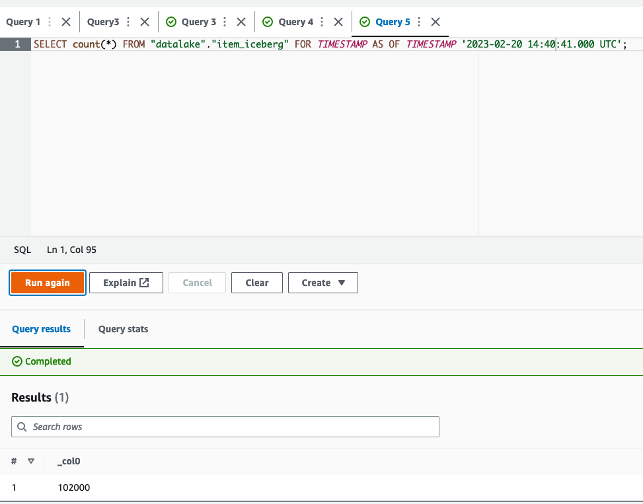
  2. On the Athena console, run the following query to count the item table records at a time before the update job, replacing <TRAVEL_TIME> with your time:
SELECT count(*) FROM "datalake"."item_iceberg" FOR TIMESTAMP AS OF TIMESTAMP <TRAVEL_TIME>;

The query will give 102,000 as a result, the expected table size before running the update job.

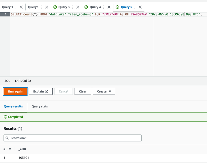
  1. Now you can run a query with a timestamp after the successful run of the update job (for example, 2023-02-20 15:06:00.000 UTC):
SELECT count(*) FROM "datalake"."item_iceberg" FOR TIMESTAMP AS OF TIMESTAMP <TRAVEL_TIME>;

The query will now give 103,101 as the size of the table at that time, after the update job successfully finished.

Additionally, you can query in Athena based on the version ID of a snapshot in Iceberg. However, for more advanced use cases, such as to roll back to a given version or to find version IDs, you can use Iceberg’s SDK or Spark on Amazon EMR.

Clean up

Complete the following steps to clean up your resources:

  1. On the Amazon S3 console, empty your buckets.
  2. On the Athena console, delete the workgroup DatalakeWorkgroup.
  3. On the EMR Studio console, stop the application datalake-app.
  4. On the AWS CloudFormation console, delete the CloudFormation stack.

Conclusion

In this post, we created a serverless transactional data lake with Iceberg tables, EMR Serverless, and Athena. We used TPC-DS sales data with 10 GB data and more than 7 million records in the fact table. We demonstrated how straightforward it is to rely on SQL and Spark to run serverless jobs for data ingestion and upserts. Moreover, we showed how to run complex BI queries directly on Iceberg tables from Athena for reporting.

You can start building your serverless transactional data lake on AWS today, and dive deep into the features and optimizations Iceberg provides to build analytics applications more easily. Iceberg can also help you in the future to improve performance and reduce costs.


About the Author

Houssem is a Specialist Solutions Architect at AWS with a focus on analytics. He is passionate about data and emerging technologies in analytics. He holds a PhD on data management in the cloud. Prior to joining AWS, he worked on several big data projects and published several research papers in international conferences and venues.

Welcome to Security Week 2023

Post Syndicated from Reid Tatoris original https://blog.cloudflare.com/welcome-to-security-week-2023/

Welcome to Security Week 2023

Welcome to Security Week 2023

Last month I had the chance to attend a dinner with 56 CISOs and CSOs across a range of banking, gaming, ecommerce, and retail companies. We rotated between tables of eight people and talked about the biggest challenges those in the group were facing, and what they were most worried about around the corner. We talk to customers every day at Cloudflare, but this was a unique opportunity to listen to customers (and non-customers) talk to each other. It was a fascinating evening and a few things stood out.

The common thread that dominated the discussions was “how do I convince my business and product teams to do the things I want them to”. Surprisingly little time was spent on specific technical challenges. No one brought up a concern about recent advanced mage cart skimmers, or about protecting their new GraphQL APIs, or how to secure two different cloud vendors at once, or about the size of DDoS attacks consistently getting larger. Over and over again the conversation came back to struggles with getting humans to do the secure thing, or to not do the insecure thing.

This instantly brought to mind a major phishing attack that Cloudflare was able to thwart last August. The attack was extremely sophisticated, using targeted text messages and an extremely professional impersonation of our Okta login page. Cloudflare did have individual employees fall for the phishing messages, because we are made up of a team of humans who are human. But we were able to thwart the attack through our own use of Cloudflare One products, and physical security keys issued to every employee that are required to access all our applications. The attacker was able to obtain compromised username and password credentials, but they could not get past the hard key requirement to log in. In 2023 phishing attacks are only getting more frequent.

Today’s security challenges are often a case of having the right tools deployed to prevent people from making mistakes. Last year when we kicked off Security Week, we talked about making a shift from protecting websites, to protecting applications. Today, the shift is from protecting applications, to protecting employees, and making sure they are protected everywhere. Just a few weeks ago, the White House released a new national cybersecurity strategy directing all agencies to “implement multi-factor authentication, gain visibility into their entire attack surface, manage authorization and access, and adopt cloud security tools”. Over the next six days you’ll read more than 30 announcements that will make it as easy as possible to do just that.

Welcome to Security Week 2023.

“The more tools you use the less secure you are”

This was a direct quote from the CISO of a large online gaming platform. Adding more vendors might seem like you are adding layers of security, but you do also open up avenues for risk. First, every third party you add by definition adds another potential vulnerability. The recent LastPass breach is a perfect example. Attackers gained access to a cloud storage service, which gave them information they used in a secondary attack to phish an employee. Second, more tools means more complexity. More systems to log into, more dashboards to check. If information is spread across multiple systems you are more likely to miss important changes. Third, the more tools you use, the less likely it is that anyone is able to master them all. If you need the person who knows the application security tool, and the person who knows the SIEM, and the person who knows the access tool to coordinate on every potential vulnerability, things will get lost in translation. Complexity is the enemy of security. Fourth, adding more tools can add a false sense of security. Simply adding a new tool can give the impression you’ve added defense in depth. But that tool only adds protection if it works, if it’s configured properly, and if people actually use it.

This week, you will hear about all of the initiatives we’ve been working on to help you solve this problem. We will announce multiple integrations that make it easier for you to deploy and manage Zero Trust anywhere, across multiple platforms, but all within the Cloudflare dashboard. We’re also extending our proven detection capabilities into new areas that will help you solve problems you couldn’t solve before, and thus allow you to get rid of additional vendors. And we’ll announce a brand new migration tool that makes it dead simple to move from those other vendors to Cloudflare.

Leverage machine learning to let humans focus on critical thinking

We all hear machine learning thrown around as a buzzword too often, but it boils down to this: computers are really good at finding patterns. When we train them on what a good pattern looks like, they can spot them really well, and spot the outliers. Humans are great at finding patterns too. But it takes us a long time, and any time we spend finding patterns distracts us from the thing that even the best AI or ML model still can’t do: critical thinking. By using machine learning to find these good and bad patterns, you can optimize the time of your most valuable people. Rather than searching for exceptions, they can focus on only those exceptions, and use their wisdom to make the hard decisions about what to do next.

Cloudflare has used machine learning to catch DDoS attacks, malicious bots, and malicious web traffic. We were able to do this differently from others because we built a unique network where we run all of our code at every single data center, on every single machine. Since we have a massive global network that is close to end users, we can run machine learning close to those users, unlike competitors who have to use centralized data centers. The result is a machine learning pipeline that runs inference in a few microseconds. That unique speed is an advantage for our customers, one we now use to run inference more than 40 million times every second.

This week, we have an entire day focused on how we are using that machine learning pipeline to build new models that will allow you to find new patterns, like fraud and API endpoints.

Our intelligence is your intelligence

In June we announced Cloudforce One, the first step in our threat operations team dedicated to turning the intelligence we gather from handling nearly 20% of Internet traffic into actionable insights. Since that launch, we’ve heard customers ask us to do more with those insights and give them easy buttons and products to take the appropriate action on their behalf. This week you’ll read multiple announcements on new ways that you can view and take action on unique Cloudflare threat intelligence. We’ll also be announcing multiple new reporting views, like being able to view more data at an account level so you can have one single lens into security trends across your entire organization.

Make it harder for humans to make mistakes

Each product, development, or business team wants to use their own tools, and wants to move as quickly as possible. For good reason! Any security that comes after the fact, and creates additional work for those teams, will be difficult to get internal buy on for. Which can lead to situations like the recent T-mobile hack where an API that was not intended to be public was exposed, discovered, and exploited. You need to meet teams where they are by making the tools they already use more secure, and preventing them from making mistakes, rather than giving them additional tasks.

In addition to making it easier to deploy our Application Security and Zero Trust products to a wider scope, you’ll also read about how we are adding new features that prevent humans from making the mistakes they always do. You’ll hear about how you can make it impossible to click on a phishing link by automatically blocking the domains that host them, prevent data from leaving regions it should never leave, give your users security alerts directly in the tools they already use, and automatically detect shadow APIs without making your developers change their development process. All of this without having to convince internal teams to make any changes to their behavior.

If you’re reading this and any part of your job involves securing an organization, I think that by the end of the week we’ll have made your job easier. With the new tools and integrations we release, you’ll be able to protect more of your infrastructure from a wider range of threats, but reduce the number of third parties you rely on. More importantly, you’ll be able to reduce the number of mistakes that the incredible humans you work with can make. I hope that helps you rest a bit easier!

Благо или бреме?

Post Syndicated from Анета Василева original https://www.toest.bg/blago-ili-breme/

За наградата „Прицкер“, културното наследство и летището в Русе – отново

Благо или бреме?

Тълпи от хора, дълги опашки, бариери и турникети, евтини сувенири и постоянен шум. Това е туристическото ежедневие на паметниците на културата в Стара Европа, независимо дали говорим за форумите в Рим, за Венеция, Барселона или Синтра.

Хора, хванати за ръце, протестират пред багери, правят плакати и подписки в социалните мрежи, говорят гневно пред камери, призовават институциите, държавата, някой, който и да е, да помогне. Това е активисткото, протестно ежедневие на архитектурното наследство в съвременния град – рушащи се сгради в Белград, горящи тютюневи складове в Пловдив, бруталистични бетонни жилищни гета в Лондон, концертни зали в Германия, едно летище в Русе.

Трябва да проверим дали сградата е паметник. Ако е – няма да купуваме, ще отидат пак години за съгласуване и двойни разходи по ремонта.

Това пък е болезнено реалистичното инвестиционно ежедневие на „наследството“, при това май не само в България.

Изобщо, културното наследство, оказва се, е проблем.

Да, то пази следите от миналото и постиженията на човешката цивилизация за следващите поколения. Да, то носи идентичност и многообразие, но пак е проблем. Скъпо е, трудно е, елитарно е, тежко институционализирано и обикновено спорно. На всичкото отгоре е навсякъде.

Но може ли културното наследство освен бреме или музеен експонат да е нещо друго – например възможност?

Опазване, реставрация и наградата „Прицкер“

В началото на март всяка година архитектурният свят очаква една новина: кой ще бъде поредният носител на най-престижната международна награда за архитектура „Прицкер“. През годините наградата е бетонирала звезди, реабилитирала е „стари майстори“ малко преди смъртта им, изненадвала е с непопулярни имена, разочаровала е или е отговаряла на очаквания и като цяло именно тя играе ролята на „съвестта“ на голямата архитектура.

На 7 март 2022 г. „Прицкер“ отиде при англичанина Дейвид Чипърфийлд – един внимателен контекстуалист,

който десетки години прави спокойни, умни сгради, съобразени с духа на мястото си и с духа на времето ни. Най-после културното наследство, консервацията и реставрацията имат своя лауреат.

Само един пример е достатъчен.

„Новият“ Neues Museum е част от Острова на музеите в Берлин, завършен точно зад „стария“ Altes Museum през 1859 г. по поръчка на Фридрих Вилхелм III и по проект на придворния архитект Фридрих Щюлер. Целта е мястото да започне да се оформя като „светилище на изкуствата и науката“. Неслучайно всички сгради приличат на антични храмове в своята версия от ХIХ век. За разлика от Altes Museum, бомбардировките през Втората световна война оставят Neues Museum в руини. В крайна сметка след няколко неуспешни опита за възстановяване сградата е изоставена.

През 1997 г. Чипърфийлд съвместно с реставратора Джулиан Харап печели международния конкурс за реконструкция на сградата. Основната цел на проекта победител е възстановяването на оригиналния обем и реставрацията на оцелелите след бомбардировките части от музея.

„Внимателна“ и „чувствителна“ реставрация е лайтмотивът на архитектурния екип.

Оригиналната останала тъкан на музея е запазена и реконструкцията е водена именно от тези следи, а също и от обемите в точната им кубатура, както е проектирана от архитект Щюлер. Основните обеми – северозападното крило, апсидата на гръцкия двор и южният купол – са изградени от рециклирани, ръчно правени тухли. Новите части – голямоформатни, предварително излети бетонни елементи – са отчетливо отделени, но въпреки това се сливат хармонично със старото. Като например впечатляващото бяло ново централно стълбище, интерпретиращо разрушеното старо, което е позиционирано в грандиозната централна зала, запазена само като тухлена обвивка, оголена от бомбардировките и дългогодишната разруха.

В зависимост от типа и нивото на разрухата архитектите търсят индивидуално решение за всяко помещение. Воден от идеята, че оригиналната структура трябва да бъде подчертавана в нейния пространствен контекст и оригинална материалност, проектът отразява загубата, без да я имитира. Но и всички травматични следи са запазени – канелираните колони със следи от пожари, дупките от куршумите по тухлените стени…

Реконструкцията на Neues Museum, както и всички намеси на Дейвид Чипърфийлд на Острова на музеите в Берлин след това (като една допълнителна, чисто нова сграда към музейния комплекс – James Simos Gallery, завършена през 2019 г.) са сред най-деликатните и в същото време най-силни послания, които архитектурата е отправяла към обществото през последните години. Да помним миналото в цялата му комплексност и многообразие като едновременно с това не се страхуваме да правим добра нова архитектура. Така наследството работи за града, за обществото и в крайна сметка – за бъдещето.

Интересното е, че няколко часа след като новината за наградата на Чипърфийлд обиколи света, тя се появи и на страницата на малкия регионален вестник „Утро“ от град Русе. Но някак си никой от журналистите във вестника не направи връзката между подхода на Чипърфийлд и една малка сграда в близкото село Щръклево.

Казусът „Русе“

Снимки на едно забележително запазено летище, доскоро напълно непознато, обикалят социалните мрежи вече две години.

Приемната сграда на Летище „Русе“ е открита през 1976 г. в близкото село Щръклево и е обявена за еталон на БГА „Балкан“. Проектирана от русенския архитект Йордан Бояджиев, тя е сред най-ярките, най-последователни откъм архитектурни решения и най-автентично запазени примери за следвоенен архитектурен модернизъм у нас. Сградата впечатлява с педантичен детайл, дръзки конструктивни решения и монументалните пластики на скулптора Галин Малакчиев.

От няколко години летището е едновременно обект на инвеститорски интерес и във фокуса на вниманието на експерти в областта на опазването на културното наследство. В началото казусът се оформя като кампания за сграда в риск, а хронологията на събитията е ясно проследима на страницата на българската секция на Docomomo International – Международната неправителствена организация за опазване на обекти на Модерното движение. Накратко:

  • През февруари 2021 г. в медиите се появява информация за инвеститорски интерес за строеж на голям логистичен парк на мястото на летището, който дори не отчита сградата на аерогарата и я показва преместена и драстично променена. „Докомомо България“ започва популяризирането на архитектурните качества на летището и работа върху регистрационен фиш за обявяването му под защита от Закона за културното наследство.
  • През декември 2021 г. Националният институт за недвижимо културно наследство съобщава, че работи по материали, подготвени от „Докомомо България“, за обявяването на Летище „Русе“ за „недвижима културна ценност“ и легитимирането му като културно наследство на модернизма на ХХ век.
  • През лятото на 2022 г. изложбата ТОТАЛПРОЕКТ на Фондация „Ново архитектурно наследство“ в РЦСИ „Топлоцентрала“, София, разказва историята на Летище „Русе“ пред най-широка публика и показва неговия „полет“ през няколко нива на архитектура и дизайн: градоустройство, пространство, конструкция, детайл, дизайн и синтез.
  • На 19 декември 2022 г. Специализираният експертен съвет към Министерството на културата (СЕСОНКЦ) гласува единодушно сградата на Летище „Русе“ да бъде обявена за „недвижима културна ценност“ от „национално значение“. По закон министърът на културата трябва в едномесечен срок да издаде заповед, с която да формализира решението, и така обектът да бъде официално защитен от събаряне или други кардинални ремонтни дейности.
  • Междувременно в края на януари 2023 г. Общинският съвет в Русе гласува почти единодушно местното летище да бъде дадено на частната фирма „Еърпорт Русе“ за следващите десет години срещу обещание за инвестиции и цялостно възраждане на аеродрума. На 27 февруари 2023 г. Община Русе обявява, че е подписано споразумение за безвъзмездно отдаване на Летище „Русе“ за първоначален срок от 24 месеца.

Очевидно е надбягването между „опазватели“ и институции. Според разследващи журналисти Община Русе е забавила умишлено обявяването на местното летище за паметник на културата. Русенското гражданско сдружение „Проект 7000“ пита Общината защо никъде в решението не се споменават архитектурната ценност на сградата и фактът, че тя е на един подпис от най-високия статут за културно наследство в държавата. Русенски депутати от „Продължаваме промяната“ обжалват решението на Община Русе. „Докомомо България“ пише призиви към министри, КАБ, САБ и медии за бързо привеждане в сила на решението на СЕСОНКЦ. Но в началото на март 2023 г. русенският сайт „Дунав мост“ ентусиазирано съобщава, че на летището вече „кипи ремонтна дейност“.

Статутът като проблем

Както казва русенският архитект Венцислав Илиев, ученик на Йордан Бояджиев и популяризатор на сградата на Летище „Русе“ пред колегите си от „Докомомо България“ през 2021 г., статутът поставя много сериозни предизвикателства пред всеки архитект, който ще се наеме да адаптира сградата към съвременните изисквания, а също и към собственика – Община Русе, и към новите концесионери. Защо? Ами защото има ограничения, проектът става по-сложен, нужни са многократно повече архитектурни усилия. Затова е по-удобно да не се дава гласност на решението за обявяване на статута.

И тук се крие основният проблем.

Статутът „недвижима културна ценност“ у нас обичайно се свързва със сложни процедури за съгласуване на строително-ремонтни дейности и други административни утежнения. И това е част от реалистичното ежедневие на културното наследство у нас. В същото време

всички са убедени, че новото ще бъде по-лошо от старото,

че без статут опазването на архитектурна ценност е невъзможно – и това обикновено е точно така. Но използването на статута като наказание и насилствена превенция е също толкова опасно, колкото липсата му – и обикновено също толкова безсмислено. Погледнете изгорелите тютюневи складове в Пловдив или Захарна фабрика в София – все признато наследство от най-висока категория.

Наследство „за спасяване“ или за развитие?

Как „спасяваме“ сградите днес? Намирам за дълбоко притеснителна дори самата идея, че културното наследство постоянно трябва да бъде „спасявано“.

Бизнесът се страхува, институциите са в ступор, а гражданското общество стои, хванато за ръце, протестира и чака безкрайните бюрократични процедури с щампа „недвижимо културно наследство“ да приключат, с надеждата за пет минути медийно внимание, което да е достатъчно за поредната кауза. Защо? Защото наследството обикновено се „спасява“.

Все си мисля, че има начин опазването да излезе от пространството на емоциите и каузите, да изплува от блатото на бюрокрацията и да стъпи на открито, при прагматизма и здравия разум.

Да приемем, че наследството е незаобиколима част от ежедневието ни.

Да осъзнаем, че то ни прави различни, по-богати и по-специални от другите. Че съвременната българска архитектура ще стане по-добра, когато старото и наследеното не се възприема като спирачка на инвестиционните интереси, а ни помага да създаваме по-богата и многопластова нова архитектура.

Има как.

Включително в Русе, на летището. Не става въпрос просто за „ремонт“ или смяна на дограма. Става дума за архитектура.

Затова се надявам сега, след обявяването на новия лауреат на наградата „Прицкер“, все по-често да говорим с думите на Дейвид Чипърфийлд:

Като архитект аз съм по някакъв начин пазител на паметта. Нашите градове са следи от историческото минало, но също така и динамични, развиващи се системи. Да, някои сгради премахваме и заменяме с други. Изборът е наш и идеята, че опазваме само най-доброто, не е достатъчна. Въпросът е да опазим характера и качествата, които отразяват богатството на еволюцията в един град.

Русе със сигурност ще стане един още по-богат град, ако не просто ремонтира, а реставрира своето летище в село Щръклево.

Disaster Recovery Solutions with AWS-Managed Services, Part 3: Multi-Site Active/Passive

Post Syndicated from Brent Kim original https://aws.amazon.com/blogs/architecture/disaster-recovery-solutions-with-aws-managed-services-part-3-multi-site-active-passive/

Welcome to the third post of a multi-part series that addresses disaster recovery (DR) strategies with the use of AWS-managed services to align with customer requirements of performance, cost, and compliance. In part two of this series, we introduced a DR concept that utilizes managed services through a backup and restore strategy with multiple Regions. The post also introduces a multi-site active/passive approach.

The multi-site active/passive approach is best for customers who have business-critical workloads with higher availability requirements over other active/passive environments. A warm-standby strategy (as in Figure 1) is more costly than other active/passive strategies, but provides good protection from downtime and data loss outside of an active/active (A/A) environment.

Warm standby

Figure 1. Warm standby

Implementing the multi-site active/passive strategy

By replicating across multiple Availability Zones in same Region, your workloads become resilient to the failure of an entire data center. Using multiple Regions provides the most resilient option to deploy workloads, which safeguards against the risk of failure of multiple data centers.

Let’s explore an application that processes payment transactions and is modernized to utilize managed services in the AWS Cloud, as in Figure 2.

Warm standby with managed services

Figure 2. Warm standby with managed services

Let’s cover each of the components of this application, as well as how managed services behave in a multisite environment.

1. Amazon Route53 – Active/Passive Failover: This configuration consists of primary resources to be available, and secondary resources on standby in the case of failure of the primary environment. You would just need to create the records and specify failover for the routing policy. When responding to queries, Amazon Route 53 includes only the healthy primary resources. If the primary record configured in the Route 53 health check shows as unhealthy, Route 53 responds to DNS queries using the secondary record.

2. Amazon EKS control plane: Amazon Elastic Kubernetes Service (Amazon EKS) control plane nodes run in an account managed by AWS. Each EKS cluster control plane is single-tenant and unique, and runs on its own set of Amazon Elastic Compute Cloud (Amazon EC2) instances. Amazon EKS is also a Regional service, so each cluster is confined to the Region where it is deployed, with each cluster being a standalone entity.

3. Amazon EKS data plane: Operating highly available and resilient applications requires a highly available and resilient data plane. It’s best practice to create worker nodes using Amazon EC2 Auto Scaling groups instead of creating individual Amazon EC2 instances and joining them to the cluster.

Figure 2 shows three nodes in the primary Region while there will only be a single node in the secondary. In case of failover, the data plane scales up to meet the workload requirements. This strategy deploys a functional stack to the secondary Region to test Region readiness before failover. You can use Velero with Portworx to manage snapshots of persistent volumes. These snapshots can be stored in an Amazon Simple Storage Service (Amazon S3) bucket in the primary Region, which is replicated to an Amazon S3 bucket in another Region using Amazon S3 cross-Region replication.

During an outage in the primary Region, Velero restores volumes from the latest snapshots in the standby cluster.

4. Amazon OpenSearch Service: With cross-cluster replication in Amazon OpenSearch Service, you can replicate indexes, mappings, and metadata from one OpenSearch Service domain to another. The domain follows an active-passive replication model where the follower index (where the data is replicated) pulls data from the leader index. Using cross-cluster replication helps to ensure recovery from disaster events and allows you to replicate data across geographically distant data centers to reduce latency.

Cross-cluster replication is available on domains running Elasticsearch 7.10 or OpenSearch 1.1 or later. Full documentation for cross-cluster replication is available in the OpenSearch documentation.

If you are using any versions prior to Elasticsearch 7.10 or OpenSearch 1.1, refer to part two of our blog series for guidance on using APIs for cross-Region replication.

5. Amazon RDS for PostgreSQL: One of the managed service offerings of Amazon Relational Database Service (Amazon RDS) for PostgreSQL is cross-Region read replicas. Cross-Region read replicas enable you to have a DR solution scaling read database workloads, and cross-Region migration.

Amazon RDS for PostgreSQL supports the ability to create read replicas of a source database (DB). Amazon RDS uses an asynchronous replication method of the DB engine to update the read replica whenever there is a change made on the source DB instance. Although read replicas operate as a DB instance that allows only read-only connections, they can be used to implement a DR solution for your production DB environment. If the source DB instance fails, you can promote your Read Replica to a standalone source server.

Using a cross-Region read replica helps ensure that you get back up and running if you experience a Regional availability issue. For more information on PostgreSQL cross-Region read replicas, visit the Best Practices for Amazon RDS for PostgreSQL Cross-Region Read Replicas blog post.

6. Amazon ElastiCache: AWS provides a native solution called Global Datastore that enables cross-Region replication. By using the Global Datastore for Redis feature, you can work with fully managed, fast, reliable, and secure replication across AWS Regions. This feature helps create cross-Region read replica clusters for ElastiCache for Redis to enable low-latency reads and DR across AWS Regions. Each global datastore is a collection of one or more clusters that replicate to one another. When you create a global datastore in Amazon ElastiCache, ElastiCache for Redis automatically replicates your data from the primary cluster to the secondary cluster. ElastiCache then sets up and manages automatic, asynchronous replication of data between the two clusters.

7. Amazon Redshift: With Amazon Redshift, there are only two ways of deploying a true DR approach: backup and restore, and an (A/A) solution. We’ll use the A/A solution as this provides a better recovery time objective (RTO) for the overall approach. The recovery point objective (RPO) is dependent upon the configured schedule of AWS Lambda functions. The application within the primary Region sends data to both Amazon Simple Notification Service (Amazon SNS) and Amazon S3, and the data is distributed to the Redshift clusters in both Regions through Lambda functions.

Amazon EKS uploads data to an Amazon S3 bucket and publishes a message to an Amazon SNS topic with a reference to the stored S3 object. S3 acts as an intermediate data store for messages beyond the maximum output limit of Amazon SNS. Amazon SNS is configured with primary and secondary Region Amazon Simple Queue Service (Amazon SQS) endpoint subscriptions. Amazon SNS supports the cross-Region delivery of notifications to Amazon SQS queues. Lambda functions deployed in the primary and secondary Region are used to poll the Amazon SQS queue in respective Regions to read the message. The Lambda functions then use the Amazon SQS Extended Client Library for Java to retrieve the Amazon S3 object referenced in the message. Once the Amazon S3 object is retrieved, the Lambda functions upload the data into Amazon Redshift.

For more on how to coordinate large messages across accounts and Regions with Amazon SNS and Amazon SQS, explore the Coordinating Large Messages Across Accounts and Regions with Amazon SNS and SQS blog post.

Conclusion

This active/passive approach covers how you can build a creative DR solution using a mix of native and non-native cross-Region replication methods. By using managed services, this strategy becomes simpler through automation of service updates, deployment using Infrastructure as a Code (IaaC), and general management of the two environments.

Related information

Want to learn more? Explore the following resources within this series and beyond!

[$] Interview: the FreeCAD Project Association

Post Syndicated from original https://lwn.net/Articles/924953/

The sustainability of free software continues to be mostly uncharted
waters. No team is the same as any other, so copying, say, the Blender Foundation’s
approach to governance will, most likely, not work for other projects. But
there is value in understanding how various non-commercial organizations
operate in order to make informed decisions for the governance of new ones.
In late 2021, the FreeCAD team
launched the FreeCAD Project
Association
(FPA) to handle the various assets that belong to this free
3D CAD project. In this interview, Yorik van Havre, a longtime FreeCAD
developer — and current president of the Association — guides us through
the process of starting and managing the FPA.

Deploying firmware at Cloudflare-scale: updating thousands of servers in more than 285 cities

Post Syndicated from Chris Howells original https://blog.cloudflare.com/deploying-firmware-at-cloudflare-scale-how-we-update-thousands-of-servers-in-more-than-285-cities/

Deploying firmware at Cloudflare-scale: updating thousands of servers in more than 285 cities

Deploying firmware at Cloudflare-scale: updating thousands of servers in more than 285 cities

As a security company, it’s critical that we have good processes for dealing with security issues. We regularly release software to our servers – on a daily basis even – which includes new features, bug fixes, and as required, security patches. But just as critical is the software which is embedded into the server hardware, known as firmware. Primarily of interest is the BIOS and Baseboard Management Controller (BMC), but many other components also have firmware such as Network Interface Cards (NICs).

As the world becomes more digital, software which needs updating is appearing in more and more devices. As well as my computer, over the last year, I have waited patiently while firmware has updated in my TV, vacuum cleaner, lawn mower and light bulbs. It can be a cumbersome process, including obtaining the firmware, deploying it to the device which needs updating, navigating menus and other commands to initiate the update, and then waiting several minutes for the update to complete.

Firmware updates can be annoying even if you only have a couple of devices. We have more than a few devices at Cloudflare. We have a huge number of servers of varying kinds, from varying vendors, spread over 285 cities worldwide. We need to be able to rapidly deploy various types of firmware updates to all of them, reliably, and automatically, without any kind of manual intervention.

In this blog post I will outline the methods that we use to automate firmware deployment to our entire fleet. We have been using this method for several years now, and have deployed firmware without interrupting our SRE team, entirely automatically.

Background

A key component of our ability to deploy firmware at scale is the iPXE, an open source boot loader. iPXE is the glue which operates between the server and operating system, and is responsible for loading the operating system after the server has completed the Power On Self Test (POST). It is very flexible and contains a scripting language. With iPXE, we can write boot scripts which query the firmware version, continue booting if the correct firmware version is deployed, or if not, boot into a flashing environment to flash the correct firmware.

We only deploy new firmware when our systems are out of production, so we need a method to coordinate deployment only on out of production systems. The simplest way to do this is when they are rebooting, because by definition they are out of production then. We reboot our entire fleet every month, and have the ability to schedule reboots more urgently if required to deal with a security issue. Regularly rebooting our fleets has many advantages. We can deploy the latest Linux kernel, base operating system, and ensure that we do not have any breaking changes in our operating system and configuration management environment that breaks on fresh boot.

Our entire fleet operates in UEFI mode. UEFI is a modern replacement for the BIOS and offers more features and more security, such as Secure Boot. A full description of all of these changes is outside the scope of this article, but essentially UEFI provides a minimal environment and shell capable of executing binaries. Secure Boot ensures that the binaries are signed with keys embedded in the system, to prevent a bad actor from tampering with our software.

How we update the BIOS

We are able to update the BIOS without booting any operating system, purely by taking advantage of features offered by iPXE and the UEFI shell. This requires a flashing binary written for the UEFI environment.

Upon boot, iPXE is started. Through iPXE’s built-in variable ${smbios/0.5.0}  it is possible to query the current BIOS version, and compare it to the latest version, and trigger a flash only if there is a mis-match.  iPXE then downloads the files required for the firmware update to a ramdisk.

The following is an example of a very basic iPXE script which performs such an action:

# Check whether the BIOS version is 2.03
iseq ${smbios/0.5.0} 2.03 || goto biosupdate
echo Nothing to do for {{ model }}
exit 0

:biosupdate
echo Trying to update BIOS/UEFI...
echo Current: ${smbios/0.5.0}
echo New: 2.03

imgfetch ${boot_prefix}/tools/x64/shell.efi || goto unexpected_error
imgfetch startup.nsh || goto unexpected_error

imgfetch AfuEfix64.efi || goto unexpected_error
imgfetch bios-2.03.bin || goto unexpected_error

imgexec shell.efi || goto unexpected_error

Meanwhile, startup.nsh contains the binary to run and command line arguments to effect the flash:

startup.nsh:

%homefilesystem%\AfuEfix64.efi %homefilesystem%\bios-2.03.bin /P /B /K /N /X /RLC:E /REBOOT

After rebooting, the machine will boot using its new BIOS firmware, version 2.03. Since ${smbios/0.5.0} now contains 2.03, the machine continues to boot and enter production.

Other firmware updates such as BMC, network cards and more

Unfortunately, the number of vendors that support firmware updates with UEFI flashing binaries is limited. There are a large number of other updates that we need to perform such as BMC and NIC.

Deploying firmware at Cloudflare-scale: updating thousands of servers in more than 285 cities

Consequently, we need another way to flash these binaries. Thankfully, these vendors invariably support flashing from Linux. Consequently we can perform flashing from a minimal Linux environment. Since vendor firmware updates are typically closed source utilities and vendors are often highly secretive about firmware flashing, we can ensure that the flashing environment does not provide an attackable surface by ensuring that the network is not configured. If it’s not on the network, it can’t be attacked and exploited.

Not being on the network means that we need to inject files into the boot process when the machine boots. We can accomplish this with an initial ramdisk (initrd), and iPXE makes it easy to add additional initrd to the boot.

Creating an initrd is as simple as creating an archive of the files using cpio using the newc archive format.

Let’s imagine we are going to flash Broadcom NIC firmware. We’ll use the bnxtnvm firmware update utility, the firmware image firmware.pkg, and a shell script called flash to automate the task.

The files are laid out in the file system like this:

cd broadcom
find .
./opt/preflight
./opt/preflight/scripts
./opt/preflight/scripts/flash
./opt/broadcom
./opt/broadcom/firmware.pkg
./opt/broadcom/bnxtnvm

Now we compress all of these files into an image called broadcom.img.

find . | cpio --quiet -H newc -o | gzip -9 -n > ../broadcom.img

This is the first step completed; we have the firmware packaged up into an initrd.

Since it’s challenging to read, say, the firmware version of the NIC, from the EFI shell, we store firmware versions as UEFI variables. These can be written from Linux via efivars, the UEFI variable file system, and then read by iPXE on boot.

An example of writing an EFI variable from Linux looks like this:

declare -r fw_path='/sys/firmware/efi/efivars/broadcom-fw-9ca25c23-368a-4c21-943f-7d91f2b76008'
declare -r efi_header='\x07\x00\x00\x00'
declare -r version='1.05'

/bin/mount -o remount,rw,nosuid,nodev,noexec,noatime none /sys/firmware/efi/efivars

# Files on efivarfs are immutable by default, so remove the immutable flag so that we can write to it: https://docs.kernel.org/filesystems/efivarfs.html
if [ -f "${fw_path}" ] ; then
    /usr/bin/chattr -i "${fw_path}"
fi

echo -n -e "${efi_header}${version}" >| "$fw_path"

Then we can write an iPXE configuration file to load the flashing kernel, userland and flashing utilities.

set cf/guid 9ca25c23-368a-4c21-943f-7d91f2b76008

iseq ${efivar/broadcom-fw-${cf/guid}} 1.05 && echo Not flashing broadcom firmware, version already at 1.05 || goto update
exit

:update
echo Starting broadcom firmware update
kernel ${boot_prefix}/vmlinuz initrd=baseimg.img initrd=linux-initramfs-modules.img initrd=broadcom.img
initrd ${boot_prefix}/baseimg.img
initrd ${boot_prefix}/linux-initramfs-modules.img
initrd ${boot_prefix}/firmware/broadcom.img

Flashing scripts are deposited into /opt/preflight/scripts and we use systemd to execute them with run-parts on boot:

/etc/systemd/system/preflight.service:

[Unit]
Description=Pre-salt checks and simple configurations on boot
Before=salt-highstate.service
After=network.target

[Service]
Type=oneshot
RemainAfterExit=yes
ExecStart=/bin/run-parts --verbose /opt/preflight/scripts

[Install]
WantedBy=multi-user.target
RequiredBy=salt-highstate.service

An example flashing script in /opt/preflight/scripts might look like:

#!/bin/bash

trap 'catch $? $LINENO' ERR
catch(){
    #error handling goes here
    echo "Error $1 occured on line $2"
}

declare -r fw_path='/sys/firmware/efi/efivars/broadcom-fw-9ca25c23-368a-4c21-943f-7d91f2b76008'
declare -r efi_header='\x07\x00\x00\x00'
declare -r version='1.05'

lspci | grep -q Broadcom
if [ $? -eq 0 ]; then
    echo "Broadcom firmware flashing starting"
    if [ ! -f "$fw_path" ] ; then
        chmod +x /opt/broadcom/bnxtnvm
        declare -r interface=$(/opt/broadcom/bnxtnvm listdev | grep "Device Interface Name" | awk -F ": " '{print $2}')
        /opt/broadcom/bnxtnvm -dev=${interface} -force -y install /opt/broadcom/BCM957414M4142C.pkg
        declare -r status=$?
        declare -r currentversion=$(/opt/broadcom/bnxtnvm -dev=${interface} device_info | grep "Package version on NVM" | awk -F ": " '{print $2}')
        declare -r expectedversion=$(echo $version | awk '{print $2}')
        if [ $status -eq 0 -a "$currentversion" = "$expectedversion" ]; then
            echo "Broadcom firmware $version flashed successfully"
            /bin/mount -o remount,rw,nosuid,nodev,noexec,noatime none /sys/firmware/efi/efivars
            echo -n -e "${efi_header}${version}" >| "$fw_path"
            echo "Created $fw_path"
        else
            echo "Failed to flash Broadcom firmware $version"
            /opt/broadcom/bnxtnvm -dev=${interface} device_info
        fi
    else
        echo "Broadcom firmware up-to-date"
    fi
else
    echo "No Broadcom NIC installed"
    /bin/mount -o remount,rw,nosuid,nodev,noexec,noatime none /sys/firmware/efi/efivars
    if [ -f "${fw_path}" ] ; then
        /usr/bin/chattr -i "${fw_path}"
    fi
    echo -n -e "${efi_header}${version}" >| "$fw_path"
    echo "Created $fw_path"
fi

if [ -f "${fw_path}" ]; then
    echo "rebooting in 60 seconds"
    sleep 60
    /sbin/reboot
fi

Conclusion

Whether you manage just your laptop or desktop computer, or a fleet of servers, it’s important to keep the firmware updated to ensure that the availability, performance and security of the devices is maintained.

If you have a few devices and would benefit from automating the deployment process, we hope that we have inspired you to have a go by making use of some basic open source tools such as the iPXE boot loader and some scripting.

Final thanks to my colleague Ignat Korchagin who did a large amount of the original work on the UEFI BIOS firmware flashing infrastructure.

The collective thoughts of the interwebz