What’s New in InsightIDR: Q4 2022 in Review

Post Syndicated from Dina Durutlic original https://blog.rapid7.com/2023/01/17/whats-new-in-insightidr-q4-2022-in-review/

What’s New in InsightIDR: Q4 2022 in Review

As we continue to empower security teams with the freedom to focus on what matters most, Q4 focused on investments and releases that contributed to that vision. With InsightIDR, Rapid7’s cloud-native SIEM and XDR solution, teams have the scale, comprehensive contextual coverage, and expertly vetted detections they need to thwart threats early in the attack chain.

This 2022 Q4 recap post offers a closer look at the recent investments and releases we’ve made over the past quarter. Here are some of the highlights:

Easy to create and manage log search, dashboards, and reports

You spoke, we listened! Per our customers, you can now create tables with multiple columns, allowing teams to see all data in one view. For example, simply add a query with a “where” clause and select a table display followed by the columns you want displayed.

Additionally, teams can reduce groupby search results with the having() clause. Customers can filter out what data is returned from groupby results with the option to layer in existing analytics function support (e.g. count, unique, max).

What’s New in InsightIDR: Q4 2022 in Review

Accelerated time to value

The InsightIDR Onboarding Progress Tracker, available for customers during their 90 day onboarding period, is a self-serve, centralized check-list of onboarding tasks with step-by-step guidance, completion statuses, and context on the “what” and “why” of each task.

No longer onboarding? No problem! We made the progress tracker available beyond the 90-day onboarding period so customers can evaluate setup progress and ensure InsightIDR is operating at full capacity to effectively detect, investigate, and respond to threats.

What’s New in InsightIDR: Q4 2022 in Review

Visibility across your modern environment

For those that leverage Palo Alto Cortex, you can now configure Palo Alto Cortex Data Lake to send activity to InsightIDR including syslog-encrypted Web Proxy, Firewall, Ingress Authentication, etc. Similarly, for customers leveraging Zscaler, you can now configure Zscaler Log Streaming Service (LSS) to receive and parse user activity and audit logs from Zscaler Private Access through the LSS.

For teams who do not have the bandwidth to set up and manage multiple event sources pertaining to Cisco Meraki, we have added support to ingest Cisco Meraki events through the Cisco Meraki API. This will enable you to deploy and add new event sources with less management.

What’s New in InsightIDR: Q4 2022 in Review

Customers can now bring data from their Government Community Cloud (GCC) and GCC High environments when setting up the Office365 event source to ensure security standards are met when processing US Government data.

Stay tuned!

We’re always working on new product enhancements and functionality to ensure your team can stay ahead of potential threats and malicious activity. Keep an eye on the Rapid7 blog and the InsightIDR release notes to keep up to date with the latest detection and response releases at Rapid7.

Build highly available streams with Amazon Kinesis Data Streams

Post Syndicated from Jeremy Ber original https://aws.amazon.com/blogs/big-data/build-highly-available-streams-with-amazon-kinesis-data-streams/

Many use cases are moving towards a real-time data strategy due to demand for real-time insights, low-latency response times, and the ability to adapt to the changing needs of end-users. For this type of workload, you can use Amazon Kinesis Data Streams to seamlessly provision, store, write, and read data in a streaming fashion. With Kinesis Data Streams, there are no servers to manage, and you can scale your stream to handle any additional throughput as it comes in.

Kinesis Data Streams offers 99.9% availability in a single AWS Region. For even higher availability, there are several strategies to explore within the streaming layer. This post compares and contrasts different strategies for creating a highly available Kinesis data stream in case of service interruptions, delays, or outages in the primary Region of operation.

Considerations for high availability

Before we dive into our example use case, there are several considerations to keep in mind when designing a highly available Kinesis Data Streams workload that relate to the business need for a particular pipeline:

  • Recovery Time Objective (RTO) is defined by the organization. RTO is the maximum acceptable delay between the interruption of service and restoration of service. This determines what is considered an acceptable time window when service is unavailable.
  • Recovery Point Objective (RPO) is defined by the organization. RPO is the maximum acceptable amount of time since the last data recovery point. This determines what is considered an acceptable loss of data between the last recovery point and the interruption of service.

In a general sense, the lower your values for RPO and RTO, the more expensive the overall solution becomes. This is because the solution needs to account for minimizing both data loss and service unavailability by having multiple instances of the service up and running in multiple Regions. This is why a big piece of high availability is the replication of data flowing through a workload. In our case, the data is replicated across Regions of Kinesis Data Streams. Conversely, the higher the RPO and RTO values are, the more complexity you introduce into your failover mechanism. This is due to the fact that the cost savings you realize by not standing up multiple instances across multiple Regions are offset by the orchestration needed to spin up these instances in the event of an outage.

In this post, we are only covering failover of a Kinesis data stream. In use cases where higher availability is required across the entire data pipeline, having failover architectures for every component (Amazon API Gateway, AWS Lambda, Amazon DynamoDB) is strongly encouraged.

The simplest approach to high availability is to start a new instance of producers, consumers, and data streams in a new Region upon service unavailability detection. The benefit here is primarily cost, but your RPO and RTO values will be higher as a result.

We cover the following strategies for highly available Kinesis Data Streams:

  • Warm standy – An architecture in which there is active replication of data from the Kinesis data stream in Region A to Region B. Consumers of the data stream are running in both Regions at all times. Recommended for use cases that can’t withstand extended downtime past their replication lag.
  • Cold standby – Active replication of data from the data stream in Region A to Region B, but consumers of the data stream in Region B are spun up when an outage in Region A is detected. Recommended for use cases that can afford some downtime as infrastructure is spun up in secondary Region. In this scenario, RPO will be similar to the warm standby strategy; however, RTO will increase.

For high availability purposes, these use cases need to replicate the data across Regions in a way that allows consumers and producers of the data stream to fail over quickly upon detection of a service unavailability and utilize the secondary Region’s stream. Let’s take an example architecture to further explain these DR strategies. We use API Gateway and Lambda to publish stock ticker information to a Kinesis data stream. The data is then retrieved by another Lambda consumer to save durably into DynamoDB for querying, alerting, and reporting. The following diagram illustrates this architecture.

the primary architecture for the post--showcasing data coming from a mobile phone to API Gateway, then AWS Lambda, then Kinesis Data Streams, Lambda again and finally publishing to a DynamoDB Table

We use this architecture with an example use case requiring the streaming workload to be highly available in the event of a Region outage. The customer can withstand an RTO of 15 minutes during an outage, because they refresh end-users’ dashboards on a 15-minute interval. The customer is sensitive to downtime and data loss, because their data will be used for historical auditing purposes, operational metrics, and dashboards for end-users. Downtime for this customer means that data isn’t able to be persisted in their database from their streaming layer, and therefore unavailable to any consuming application. For this use case, data can be retried up to 5 minutes from our Lambda function before failing over to the new Region. Consumers are considered unavailable when the stream is unavailable, and can scale up in the secondary Region to account for any backlog of events.

How might we approach making a Kinesis data stream highly available for this use case?

Warm standby pattern

The following architecture diagram illustrates the warm standby high availability pattern for Kinesis Data Streams.

warm standby pattern showcasing data being replicated between a kinesis data stream in one region to another

image showcasing the warm standby failover--where data from first lambda begins replicating to secondary region KDA

The warm standby architectural pattern involves running a Kinesis data stream both in the primary and secondary Region, along with consumers and downstream destinations of the primary Region’s streaming layer being replicated as well. Sources are configured to automatically fail over to the secondary Region in the case of service unavailability in the first Region. We dive into details of how to achieve this in the client failover section of this post. Data is replicated across Regions from the data stream in the primary Region to the secondary Region. This is done instead of having the sources publish to both Regions to avoid any consistency issues between the streams in the two Regions.

Although this architectural pattern gives very high availability, it’s also the most expensive option because we’re duplicating virtually the entire streaming layer across two Regions. For business use cases that can’t withstand extended data loss or withstand downtime, this may be the best option for them. From an RTO perspective, this architectural pattern ensures there will be no downtime. There is some nuance in the RPO metric in that it depends heavily on the replication lag. In the event of the primary stream becoming unavailable, whatever data hasn’t yet been replicated may be unavailable in the secondary Region. This data won’t be considered lost, but may be unavailable for consumption until the primary stream becomes available again. This method also can result in events being out of order.

For business needs that can’t tolerate this level of record unavailability, consider retaining data on the producer for the purposes of publishing to an available stream when available, or rewinding against the source for the producer if possible so that data stuck in the primary Region can be resent to the secondary stream upon failover. We cover this consideration in the client failover section of this post.

Cold standby pattern

The following architecture diagram illustrates the cold standby high availability pattern for Kinesis Data Streams.

active passive pattern for kinesis data streams

The cold standby architectural pattern involves running a data stream both in the primary and secondary Region, and spinning up the downstream resources like a stream consumer and destination for streams when a service interruption is detected—passive mode. Just like the warm standby pattern, sources are configured to automatically fail over to the secondary Region in the case of service unavailability in the first Region. Likewise, data is replicated across Regions from the data stream in the primary Region to the secondary Region.

The primary benefit this architectural pattern provides is cost efficiency. By not running consumers at all times, this effectively reduces your costs significantly compared to the warm standby pattern. However, this pattern may introduce some data unavailability for downstream systems while the secondary Region infrastructure is provisioned. Additionally, depending on replication lag, some records may be unavailable, as discussed in the warm standby pattern. It should be noted that depending on how long it takes to spin up resources, it may take some time for consumers to reprocess the data in the secondary Region, and latency can be introduced when failing over. Our implementation assumes a minimal replication lag and that downstream systems have the ability to reprocess a configurable amount of data to catch up to the tip of the stream. We discuss approaches to spinning these resources up in the client failover section, but one possible approach to this would be using an AWS CloudFormation template that spins these resources up on service unavailability detection.

For business needs that can tolerate some level of data unavailability and can accept interruptions while the new infrastructure in the secondary Region is spun up, this is an option to consider both from a cost perspective and an RPO/RTO perspective. The complexity of spinning up resources upon detecting service unavailability is offset by the lower cost of the overall solution.

Which pattern makes sense for our use case?

Let’s revisit the use case described earlier to identify which of the strategies best meets our needs. We can extract the pieces of information from the customer’s problem statement to identify that they need a high availability architecture that:

  • Can’t withstand extended amounts of data loss
  • Must resume operations within 15 minutes of service interruption identification

This criterion tells us that their RPO is close to zero, and their RTO is 15 minutes. From here, we can determine that the cold standby architecture with data replication provides us limited data loss, and the maximum downtime will be determined by the time it takes to provision consumers and downstream destinations in the secondary Region.

Let’s dive deeper into the implementation details of each of the core phases of high availability, including an implementation guide for our use case.

Launch AWS CloudFormation resources

If you want to follow along with our code samples, you can launch the following CloudFormation stack and follow the instructions in order to simulate the cold standby architecture referenced in this post.

Launch Stack

For purposes of the Kinesis Data Streams high availability setup demo, we use us-west-2 as the primary Region and us-east-2 as the failover Region. While deploying this solution in your own account, you can choose your own primary and failover Regions.

  1. Deploy the supplied CloudFormation template in failover Region us-east-2.

Make sure you specify us-east-2 as the value for the FailoverRegion parameter in the CloudFormation template.

  1. Deploy the supplied CloudFormation template in primary Region us-west-2.

Make sure you specify us-east-2 as the value for the FailoverRegion parameter in the CloudFormation template.

In steps 1 and 2, we deployed the following resources in the primary and failover Regions:

  1. KDS-HA-Stream – AWS::Kinesis::Stream (primary and failover Region)
  2. KDS-HA-ProducerLambda – AWS::Lambda::Function (primary Region)
  3. KDS-HA-ConsumerLambda – AWS::Lambda::Function (primary and failover Region)
  4. KDS-HA-ReplicationAgentLambda – AWS::Lambda::Function (primary Region)
  5. KDS-HA-FailoverLambda – AWS::Lambda::Function (primary Region)
  6. ticker-prices – AWS::DynamoDB::GlobalTable (primary and failover Region)

The KDS-HA-Stream Kinesis data stream is deployed in both Regions. An enhanced fan-out consumer of the KDS-HA-Stream stream KDS-HA-ReplicationAgentLambda in the primary Region is responsible for replicating messages to the data stream in the failover Region.

KDS-HA-ConsumerLambda is a Lambda function consuming messages out of the KDS-HA-Stream stream and persisting data into a DynamoDB table after preprocessing.

You can inspect the content of the ticker-prices DynamoDB table in the primary and failover Region. Note that last_updated_region attribute shows us-west-2 as its value because it’s the primary Region.

Replication

When deciding how to replicate data from a data stream in Region A to a data stream in Region B, there are several strategies that involve a consumer reading data off of the primary stream and sending that data cross-Region to the secondary data stream. This would act as a replicator service, responsible for copying the data between the two streams, maintaining a relatively low latency to replicate and ensuring data isn’t lost during this replication.

Because replication off of a shared throughput data stream could impact the flow of data in a production workload, we recommend using the enhanced fan-out feature of Kinesis Data Streams consumers to ensure replication doesn’t have an impact on consumption latency.

The replication strategy implemented in this post features asynchronous replication, meaning that the replication process doesn’t block any standard data flow in the primary stream. Synchronous replication would be a safer approach to guarantee replication and avoid data loss; however, this isn’t possible without a service-side implementation.

The following image shows a timeline of data flow for the cold standby architecture, with data being replicated as soon as it’s published.

Lambda replication

Lambda can treat a Kinesis data stream as an event source, which will funnel events from your data stream into a Lambda function. This Lambda function then receives and forwards these events across Regions to your data stream in a secondary Region. Lambda functions allow you to utilize best streaming practices such as retries of records that encounter errors, bisect on error functionality, and using the Lambda parallelization factor; using more instances of your Lambda function than you have available shards can help process records faster.

This Lambda function is at the crux of the architecture for high availability; it’s responsible solely for sending data across Regions, and it also has the best capability to monitor the replication progress. Important metrics to monitor for Lambda replication include IteratorAge, which indicates how old the last record in the batch was when it finished processing. A high IteratorAge value indicates that the Lambda function is falling behind and therefore is not keeping up with data ingestion for replication purposes. A high IteratorAge can lead to a higher RPO and the higher likelihood of data unavailability when a passive failover happens.

We use the following sample Lambda function in our CloudFormation template to replicate data across Regions:

import json
import boto3
import random
import os
import base64


def lambda_handler(event, context):
    client = boto3.client("kinesis", region_name=os.environ["FAILOVER_REGION"])
    records = []

    for record in event["Records"]:
        records.append(
            {
                "PartitionKey": record["kinesis"]["partitionKey"],
                "Data": base64.b64decode(record["kinesis"]["data"]).decode("utf-8"),
            }
        )
    response = client.put_records(Records=records, StreamName="KDS-HA-Stream")
    if response["FailedRecordCount"] > 0:
        print("Failed replicating data: " + json.dumps(response))
        raise Exception("Failed replicating data!")

The Lambda replicator in the CloudFormation template is configured to read from the data stream in the primary Region.

The following code contains the necessary AWS Identity and Access Management (IAM) permissions for Lambda, giving access for the Lambda function to assume this role. All actions are permitted on data streams and DynamoDB. In the principal of least privilege, it’s recommended to restrict this to the necessary streams in a production environment.

      AssumeRolePolicyDocument:
        Version: 2012-10-17
        Statement:
          - Effect: Allow
            Principal:
              Service:
                - lambda.amazonaws.com
            Action:
              - 'sts:AssumeRole'
      Path: /
      Policies:
        - PolicyName: root
          PolicyDocument:
            Version: 2012-10-17
            Statement:
              - Effect: Allow
                Action:
                  - 'kinesis:DescribeStream'
                  - 'kinesis:DescribeStreamSummary'
                  - 'kinesis:GetRecords'
                  - 'kinesis:GetShardIterator'
                  - 'kinesis:ListShards'
                  - 'kinesis:ListStreams'
                  - 'kinesis:SubscribeToShard'
                  - 'kinesis:PutRecords'
                Resource:
                  - 'arn:aws:kinesis:*:*:stream/KDS-HA-Stream'
                  - 'arn:aws:kinesis:*:*:stream/KDS-HA-Stream/consumer/KDS-HA-Stream-EFO-Consumer:*'
      ManagedPolicyArns:
        - 'arn:aws:iam::aws:policy/CloudWatchLogsFullAccess'
 

Health check

A generalized strategy for determining when to consider our data stream unavailable involves the use of Amazon CloudWatch metrics. We use the metrics coming off of our Lambda producer and consumer in order to assess the availability of our data stream. While producing to a data stream, an error might appear as one of the following responses back from the data stream: PutRecord or PutRecords returns an AmazonKinesisException 500 or AmazonKinesisException 503 error. When consuming from a data stream, an error might appear as one of the following responses back from the data stream: SubscribeToShard.Success or GetRecords returns an AmazonKinesisException 500 or AmazonKinesisException 503.

We can calculate our effective error rate based on PutRecord.Success and GetRecord.Success. An average error rate of 1% or higher over a time window of 5 minutes, for example, could indicate that there is an issue with the data stream, and we may want to fail over. In our CloudFormation template, this error rate threshold as well as time window are configurable, but by default we check for an error rate of 1% in the last 5 minutes to trigger a failover of our clients.

Client failover

When a data stream is deemed to be unreachable, we must now take action to keep our system available and reachable for clients on both ends of the interaction. This means for producers following the cold standby high availability architecture, we change the destination stream where the producer was writing. If high availability and failover of data producers and consumers isn’t a requirement of a given use case, a different architecture would be a better fit.

Prior to failover, the producer may have been delivering data to a stream in Region A, but we now automatically update the destination to be the stream in Region B. For different clients, the methodology of updating the producer will be different, but for ours, we store the active destination for producers in the Lambda environment variables from AWS CloudFormation and update our Lambda functions dynamically on health check failure scenarios.

For our use case, we use the maximum consumer lag time (iteratorAge) plus some buffer to influence the starting position of the failover consumer. This allows us to ensure that the consumer in the secondary Region doesn’t skip records that haven’t been processed in the originating Region, but some data overlap may occur. Note that some duplicates in the downstream system may be introduced, and having an idempotent sink or some method of handling duplicates must be implemented in order to avoid duplicate-related isssues.

In the case where data is successfully written to a data stream but is unable to be consumed from the stream, the data will not be replicated and therefore be unavailable in the second Region. The data will be durably stored in the primary data stream until it comes back online and can be read from. Note that if the stream is unavailable for a longer period of time than your total data retention period on the data stream, this data will be lost. Data retention for Kinesis Data Streams can be retrospectively increased up to 1 year.

For consumers in a cold standby architecture, upon failure detection, the consumer will be disabled or shut down, and the same consumer instance will be spun up in the secondary Region to consume from the secondary data stream. On the consumer side, we assume that the consumer application is stateless in our provided solution. If your application requires state, you can migrate or preload the application state via Amazon Simple Storage Service (Amazon S3) or a database. For a stateless application, the most important aspect of failover is the starting position.

In the following timeline, we can see that at some point, the stream in Region A was deemed unreachable.

The consumer application in Region A was reading data at time t10, and when it fails over to the secondary Region (B), it reads starting at t5 (5 minutes before the current iteratorAgeMilliseconds). This ensures that data isn’t skipped by the consumer application. Keep in mind that there may be some overlap in records in the downstream destinations.

In the provided cold standby AWS CloudFormation example, we can manually trigger a failover with the AWS Command Line Interface (AWS CLI). In the following code, we manually fail over to us-east-2:

aws lambda invoke --function-name KDS-HA-FailoverLambda --cli-binary-format raw-in-base64-out --payload '{}' response.json --region us-west-2

After a few minutes, you can inspect the content of the ticker-prices DynamoDB table in the primary and failover Region. Note that the last_updated_region attribute shows us-east-2 as its value because it’s failed over to the us-east-2 Region.

Failback

After an outage or service unavailability is deemed to be resolved, the next logical step is to reorient your clients back to their original operating Regions. Although it may be tempting to automate this procedure, a manual failback approach during off-business hours when minimal production disruption will take place makes more sense.

In the following images, we can visualize the timeline with which consumer applications are failed back to the original Region.

The producer switches back to the original Region, and we wait for the consumer in Region B to reach 0 lag. At this point, the consumer application in Region B is disabled, and replication to Region B is resumed. We have now returned to our normal state of processing messages as shown in the replication section of this post.

In our AWS CloudFormation setup, we perform a failback with the following steps:

  1. Re-enable the event source mapping and start consuming messages from the primary Region at the latest position:
aws lambda create-event-source-mapping --function-name KDS-HA-ConsumerLambda --batch-size 100 --event-source-arn arn:aws:kinesis:us-west-2:{{accountId}}:stream/KDS-HA-Stream --starting-position LATEST --region us-west-2
  1. Switch the producer back to the primary Region:
aws lambda update-function-configuration --function-name KDS-HA-ProducerLambda --environment "Variables={INPUT_STREAM=KDS-HA-Stream,PRODUCING_TO_REGION=us-west-2}" --region us-west-2
  1. In the failover Region (us-east-2), wait for your data stream’s GetRecords max iterator age (in milliseconds) CloudWatch metric to report 0 as a value. We’re waiting for the consumer Lambda function to catch up with all produced messages.
  2. Stop consuming messages from the failover Region.
  3. Run the following AWS CLI command and grab the UUID from the response, which we use to delete the existing event source mapping. Make sure you’re picking event source mapping for the Lambda function KDS-HA-ConsumerLambda.
aws lambda list-event-source-mappings --region us-east-2
aws lambda delete-event-source-mapping --uuid {{UUID}} --region us-east-2
  1. Restart the replication agent in the primary Region.
  2. Run following AWS CLI command, and capture ConsumerARN from the response:
aws kinesis list-stream-consumers --stream-arn arn:aws:kinesis:us-west-2:{{accountId}}:stream/KDS-HA-Stream --region us-west-2
aws lambda create-event-source-mapping --function-name KDS-HA-ReplicationAgentLambda --batch-size 100 --event-source-arn {{ConsumerARN}} --starting-position LATEST --region us-west-2

When this is complete, you can observe the same data stream metrics—the number of records in and out per second, consumer lag metrics, and number of errors as described in the health check section of this post—to ensure that each of the components has resumed processing data in the original Region. We can also take note of the data landing in DynamoDB, which displays which Region data is being updated from in order to determine the success of our failback procedure.

We recommend for any streaming workload that can’t withstand extended data loss or downtime to implement some form of cross-Region high availability in the unlikely event of service unavailability. These recommendations can help you determine which pattern is right for your use case.

Clean up

To avoid incurring future charges, complete the following steps:

  1. Delete the CloudFormation stack from primary Region us-west-2.
  2. Delete the CloudFormation stack from failover Region us-east-2.
  3. List all event source mappings in primary Region us-west-2 using the aws lambda list-event-source-mappings --region us-west-2 command and note the UUIDs of the event source mappings tied to the KDS-HA-ConsumerLambda and KDS-HA-ReplicationAgentLambda Lambda functions.
  4. Delete event source mappings in primary Region us-west-2 tied to the KDS-HA-ConsumerLambda and KDS-HA-ReplicationAgentLambda Lambda functions using the aws lambda delete-event-source-mapping --uuid {{UUID}} --region us-west-2 command and UUIDs noted in the previous step.

Conclusion

Building highly available Kinesis data streams across multiple Regions is multi-faceted, and all aspects of your RPO, RTO, and operational costs need to be carefully considered. The code and architecture discussed in this post is one of many different architectural patterns you can choose for your workloads, so make sure to choose the appropriate architecture based on the criteria for your specific requirements.

To learn more about Kinesis Data Streams, we have a getting started guide as well as a workshop to walk through all the integrations with Kinesis Data Streams. You can also contact your AWS Solutions Architects, who can be of assistance alongside your high availability journey.


About the Authors

Jeremy Ber has been working in the telemetry data space for the past 7 years as a Software Engineer, Machine Learning Engineer, and most recently a Data Engineer. In the past, Jeremy has supported and built systems that stream in terabytes of data per day, and process complex machine learning algorithms in real time. At AWS, he is a Senior Streaming Specialist Solutions Architect supporting both Amazon MSK and Amazon Kinesis.

Pratik Patel is a Sr Technical Account Manager and streaming analytics specialist. He works with AWS customers and provides ongoing support and technical guidance to help plan and build solutions using best practices, and proactively helps keep customer’s AWS environments operationally healthy.

Build near real-time logistics dashboards using Amazon Redshift and Amazon Managed Grafana for better operational intelligence

Post Syndicated from Paul Villena original https://aws.amazon.com/blogs/big-data/build-near-real-time-logistics-dashboards-using-amazon-redshift-and-amazon-managed-grafana-for-better-operational-intelligence/

Amazon Redshift is a fully managed data warehousing service that is currently helping tens of thousands of customers manage analytics at scale. It continues to lead price-performance benchmarks, and separates compute and storage so each can be scaled independently and you only pay for what you need. It also eliminates data silos by simplifying access to your operational databases, data warehouse, and data lake with consistent security and governance policies.

With the Amazon Redshift streaming ingestion feature, it’s easier than ever to access and analyze data coming from real-time data sources. It simplifies the streaming architecture by providing native integration between Amazon Redshift and the streaming engines in AWS, which are Amazon Kinesis Data Streams and Amazon Managed Streaming for Apache Kafka (Amazon MSK). Streaming data sources like system logs, social media feeds, and IoT streams can continue to push events to the streaming engines, and Amazon Redshift simply becomes just another consumer. Before Amazon Redshift streaming was available, we had to stage the streaming data first in Amazon Simple Storage Service (Amazon S3) and then run the copy command to load it into Amazon Redshift. Eliminating the need to stage data in Amazon S3 results in faster performance and improved latency. With this feature, we can ingest hundreds of megabytes of data per second and have a latency of just a few seconds.

Another common challenge for our customers is the additional skill required when using streaming data. In Amazon Redshift streaming ingestion, only SQL is required. We use SQL to do the following:

  • Define the integration between Amazon Redshift and our streaming engines with the creation of external schema
  • Create the different streaming database objects that are actually materialized views
  • Query and analyze the streaming data
  • Generate new features that are used to predict delays using machine learning (ML)
  • Perform inferencing natively using Amazon Redshift ML

In this post, we build a near real-time logistics dashboard using Amazon Redshift and Amazon Managed Grafana. Our example is an operational intelligence dashboard for a logistics company that provides situational awareness and augmented intelligence for their operations team. From this dashboard, the team can see the current state of their consignments and their logistics fleet based on events that happened only a few seconds ago. It also shows the consignment delay predictions of an Amazon Redshift ML model that helps them proactively respond to disruptions before they even happen.

Solution overview

This solution is composed of the following components, and the provisioning of resources is automated using the AWS Cloud Development Kit (AWS CDK):

  • Multiple streaming data sources are simulated through Python code running in our serverless compute service, AWS Lambda
  • The streaming events are captured by Amazon Kinesis Data Streams, which is a highly scalable serverless streaming data service
  • We use the Amazon Redshift streaming ingestion feature to process and store the streaming data and Amazon Redshift ML to predict the likelihood of a consignment getting delayed
  • We use AWS Step Functions for serverless workflow orchestration
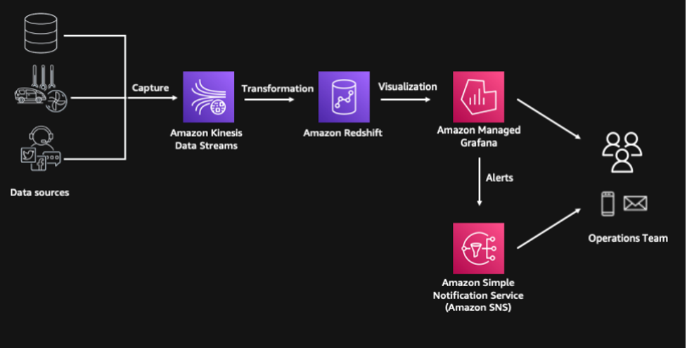
  • The solution includes a consumption layer built on Amazon Managed Grafana where we can visualize the insights and even generate alerts through Amazon Simple Notification Service (Amazon SNS) for our operations team

The following diagram illustrates our solution architecture.

Prerequisites

The project has the following prerequisites:

Sample deployment using the AWS CDK

The AWS CDK is an open-source project that allows you to define your cloud infrastructure using familiar programming languages. It uses high-level constructs to represent AWS components to simplify the build process. In this post, we use Python to define the cloud infrastructure due to its familiarity to many data and analytics professionals.

Clone the GitHub repository and install the Python dependencies:

git clone https://github.com/aws-samples/amazon-redshift-streaming-workshop
cd amazon-redshift-streaming-workshop
python3 -m venv .venv
source .venv/bin/activate
pip install -r requirements.txt

Next, bootstrap the AWS CDK. This sets up the resources required by the AWS CDK to deploy into the AWS account. This step is only required if you haven’t used the AWS CDK in the deployment account and Region.

cdk bootstrap

Deploy all stacks:

cdk deploy IngestionStack 
cdk deploy RedshiftStack 
cdk deploy StepFunctionStack

The entire deployment time takes 10–15 minutes.

Access streaming data using Amazon Redshift streaming ingestion

The AWS CDK deployment provisions an Amazon Redshift cluster with the appropriate default IAM role to access the Kinesis data stream. We can create an external schema to establish a connection between the Amazon Redshift cluster and the Kinesis data stream:

CREATE EXTERNAL SCHEMA ext_kinesis FROM KINESIS
IAM_ROLE default;

For instructions on how to connect to the cluster, refer to Connecting to the Redshift Cluster.

We use a materialized view to parse data in the Kinesis data stream. In this case, the whole payload is ingested as is and stored using the SUPER data type in Amazon Redshift. Data stored in streaming engines is usually in semi-structured format, and the SUPER data type provides a fast and efficient way to analyze semi-structured data within Amazon Redshift.


See the following code:

CREATE MATERIALIZED VIEW consignment_stream AS
SELECT approximate_arrival_timestamp,
JSON_PARSE(from_varbyte(kinesis_data, 'utf-8')) as consignment_data FROM ext_kinesis.consignment_stream
WHERE is_utf8(kinesis_data)
AND is_valid_json(from_varbyte(kinesis_data, 'utf-8'));

Refreshing the materialized view invokes Amazon Redshift to read data directly from the Kinesis data stream and load it into the materialized view. This refresh can be done automatically by adding the AUTO REFRESH clause in the materialized view definition. However, in this example, we are orchestrating the end-to-end data pipeline using AWS Step Functions.

REFRESH MATERIALIZED VIEW consignment_stream;

Now we can start running queries against our streaming data and unify it with other datasets like logistics fleet data. If we want to know the distribution of our consignments across different states, we can easily unpack the contents of the JSON payload using the PartiQL syntax.

SELECT cs.consignment_data.origin_state::VARCHAR,
COUNT(1) number_of_consignments,
AVG(on_the_move) running_fleet,
AVG(scheduled_maintenance + unscheduled_maintenance) under_maintenance
FROM consignment_stream cs
INNER JOIN fleet_summary fs
on TRIM(cs.consignment_data.origin_state::VARCHAR) = fs.vehicle_location
GROUP BY 1

Generate features using Amazon Redshift SQL functions

The next step is to transform and enrich the streaming data using Amazon Redshift SQL to generate additional features that will be used by Amazon Redshift ML for its predictions. We use date and time functions to identify the day of the week, and calculate the number of days between the order date and target delivery date.

We also use geospatial functions, specifically ST_DistanceSphere, to calculate the distance between origin and destination locations. The GEOMETRY data type within Amazon Redshift provides a cost-effective way to analyze geospatial data such as longitude and latitudes at scale. In this example, the addresses have already been converted to longitude and latitude. However, if you need to perform geocoding, you can integrate Amazon Location Services with Amazon Redshift using user-defined functions (UDFs). On top of geocoding, Amazon Location Service also allows you to more accurately calculate route distance between origin and destination, and even specify waypoints along the way.

We use another materialized view to persist these transformations. A materialized view provides a simple yet efficient way to create data pipelines using its incremental refresh capability. Amazon Redshift identifies the incremental changes from the last refresh and only updates the target materialized view based on these changes. In this materialized view, all our transformations are deterministic, so we expect our data to be consistent when going through a full refresh or an incremental refresh.


See the following code:

CREATE MATERIALIZED VIEW consignment_transformed AS
SELECT
consignment_data.consignmentid::INT consignment_id,
consignment_data.consignment_date::TIMESTAMP consignment_date,
consignment_data.delivery_date::TIMESTAMP delivery_date,
consignment_data.origin_state::VARCHAR origin_state,
consignment_data.destination_state::VARCHAR destination_state,
consignment_data.revenue::FLOAT revenue,
consignment_data.cost::FLOAT cost,
DATE_PART(dayofweek, consignment_data.consignment_date::TIMESTAMP)::INT day_of_week,
DATE_PART(hour, consignment_data.consignment_date::TIMESTAMP)::INT "hour",
DATEDIFF(days,
consignment_data.consignment_date::TIMESTAMP,
consignment_data.delivery_date::TIMESTAMP
)::INT days_to_deliver,
(ST_DistanceSphere(
ST_Point(consignment_data.origin_lat::FLOAT, consignment_data.origin_long::FLOAT),
ST_Point(consignment_data.destination_lat::FLOAT, consignment_data.destination_long::FLOAT)
) / 1000 --convert to km
) delivery_distance
FROM consignment_stream;

Predict delays using Amazon Redshift ML

We can use this enriched data to make predictions on the delay probability of a consignment. Amazon Redshift ML is a feature of Amazon Redshift that allows you to use the power of Amazon Redshift to build, train, and deploy ML models directly within your data warehouse.

The training of a new Amazon Redshift ML model has been initiated as part of the AWS CDK deployment using the CREATE MODEL statement. The training dataset is defined in the FROM clause, and TARGET defines which column the model is trying to predict. The FUNCTION clause defines the name of the function that is used to make predictions.

CREATE MODEL ml_delay_prediction -- already executed by CDK
FROM (SELECT * FROM ext_s3.consignment_train)
TARGET probability
FUNCTION fnc_delay_probabilty
IAM_ROLE default
SETTINGS (
MAX_RUNTIME 1800, --seconds
S3_BUCKET '<ingestionstack-s3bucketname>' --replace S3 bucket name
)

This simplified model is trained using historical observations, and the training process takes around 30 minutes to complete. You can check the status of the training job by running the SHOW MODEL statement:

SHOW MODEL ml_delay_prediction;

When the model is ready, we can start making predictions on new data that is streamed into Amazon Redshift. Predictions are generated using the Amazon Redshift ML function that was defined during the training process. We pass the calculated features from the transformed materialized view into this function, and the prediction results populate the delay_probability column.

This final output is persisted into the consignment_predictions table, and Step Functions is orchestrating the ongoing incremental data load into this target table. We use a table for the final output, instead of a materialized view, because ML predictions have randomness involved and it may give us non-deterministic results. Using a table gives us more control on how data is loaded.


See the following code:

CREATE TABLE consignment_predictions AS
SELECT *, fnc_delay_probability(
day_of_week, "hour", days_to_deliver, delivery_distance) delay_probability
FROM consignment_transformed;

Create an Amazon Managed Grafana dashboard

We use Amazon Managed Grafana to create a near real-time logistics dashboard. Amazon Managed Grafana is a fully managed service that makes it easy to create, configure, and share interactive dashboards and charts for monitoring your data. We can also use Grafana to set up alerts and notifications based on specific conditions or thresholds, allowing you to quickly identify and respond to issues.

The high-level steps in setting up the dashboard are as follows:

  1. Create a Grafana workspace.
  2. Set up Grafana authentication using AWS IAM Identity Center (successor to AWS Single Sign-On) or using direct SAML integration.
  3. Configure Amazon Redshift as a Grafana data source.
  4. Import the JSON file for the near real-time logistics dashboard.

A more detailed set of instructions is available in the GitHub repository for your reference.

Clean up

To avoid ongoing charges, delete the resources deployed. Access the Amazon Linux 2 environment and run the AWS CDK destroy command. Delete the Grafana objects related to this deployment.

cd amazon-redshift-streaming-workshop
source .venv/bin/activate
cdk destroy –all

Conclusion

In this post, we showed how easy it is to build a near real-time logistics dashboard using Amazon Redshift and Amazon Managed Grafana. We created an end-to-end modern data pipeline using only SQL. This shows how Amazon Redshift is a powerful platform for democratizing your data—it enables a wide range of users, including business analysts, data scientists, and others, to work with and analyze data without requiring specialized technical skills or expertise.

We encourage you to explore what else can be achieved with Amazon Redshift and Amazon Managed Grafana. We also recommend you visit the AWS Big Data Blog for other useful blog posts on Amazon Redshift.


About the Author

Paul Villena is an Analytics Solutions Architect in AWS with expertise in building modern data and analytics solutions to drive business value. He works with customers to help them harness the power of the cloud. His areas of interests are infrastructure-as-code, serverless technologies and coding in Python.

AWS achieves HDS certification in two additional Regions

Post Syndicated from Janice Leung original https://aws.amazon.com/blogs/security/aws-achieves-hds-certification-in-two-additional-regions/

We’re excited to announce that two additional AWS Regions—Asia Pacific (Jakarta) and Europe (Milan)—have been granted the Health Data Hosting (Hébergeur de Données de Santé, HDS) certification. This alignment with HDS requirements demonstrates our continued commitment to adhere to the heightened expectations for cloud service providers. AWS customers who handle personal health data can use HDS-certified Regions with confidence to manage their workloads.

The following 18 Regions are in scope for this certification:

  • US East (Ohio)
  • US East (Northern Virginia)
  • US West (Northern California)
  • US West (Oregon)
  • Asia Pacific (Jakarta)
  • Asia Pacific (Seoul)
  • Asia Pacific (Mumbai)
  • Asia Pacific (Singapore)
  • Asia Pacific (Sydney)
  • Asia Pacific (Tokyo)
  • Canada (Central)
  • Europe (Frankfurt)
  • Europe (Ireland)
  • Europe (London)
  • Europe (Milan)
  • Europe (Paris)
  • Europe (Stockholm)
  • South America (São Paulo)

Introduced by the French governmental agency for health, Agence Française de la Santé Numérique (ASIP Santé), the HDS certification aims to strengthen the security and protection of personal health data. Achieving this certification demonstrates that AWS provides a framework for technical and governance measures to secure and protect personal health data, governed by French law.

Independent third-party auditors evaluated and certified AWS on January 13, 2023. The Certificate of Compliance that demonstrates AWS compliance status is available on the Agence du Numérique en Santé (ANS) website and AWS Artifact. AWS Artifact is a self-service portal for on-demand access to AWS compliance reports. Sign in to AWS Artifact in the AWS Management Console, or learn more at Getting Started with AWS Artifact.

For up-to-date information, including when additional Regions are added, see the AWS Compliance Programs page, and choose HDS.

AWS strives to continuously bring services into the scope of its compliance programs to help you meet your architectural and regulatory needs. If you have questions or feedback about HDS compliance, reach out to your AWS account team.

To learn more about our compliance and security programs, see AWS Compliance Programs. As always, we value your feedback and questions; reach out to the AWS Compliance team through the Contact Us page.

If you have feedback about this post, submit comments in the Comments section below.

Want more AWS Security news? Follow us on Twitter.

Author

Janice Leung

Janice is a security audit program manager at AWS, based in New York. She leads security audits across Europe and previously worked in security assurance and technology risk management in the financial industry for 11 years.

Firefox 109 released

Post Syndicated from original https://lwn.net/Articles/920219/

Version
109.0
of the Firefox browser has been released. The headline feature
this time is the enabling of Manifest
Version 3 support
— a new extension mechanism that, among other
things, gives a higher degree of control over what extensions can do.

MV3 also ushers an exciting user interface change in the form of
the new extensions button (already available on Firefox
Nightly). This will give users direct control over which extensions
can access specific web sites.
Users are able to review, grant, or revoke MV3 extension access to
any website.

New Dell PowerEdge Servers with 4th Gen Intel Xeon Scalable Sapphire Rapids Launched

Post Syndicated from Cliff Robinson original https://www.servethehome.com/new-dell-poweredge-servers-with-4th-gen-intel-xeon-scalable-sapphire-rapids-launched/

Dell PowerEdge gets a 4th Gen Intel Xeon Scalable update and finally proper NVIDIA GPU platforms for AI and ML deployments

The post New Dell PowerEdge Servers with 4th Gen Intel Xeon Scalable Sapphire Rapids Launched appeared first on ServeTheHome.

Gartner® Report: Questions to Ask When Selecting an MDR Provider

Post Syndicated from Aaron Wells original https://blog.rapid7.com/2023/01/17/gartner-r-report-questions-to-ask-when-selecting-an-mdr-provider/

Measuring against the right criteria

Gartner® Report: Questions to Ask When Selecting an MDR Provider

The “right” criteria is whatever works to further your security organization’s specific needs in detection and response (D&R). There’s only so much budget to go around—and successfully obtaining a significant year-over-year increase can be rare. The last thing anyone wants to be known for is depleting that budget on a service provider that doesn’t deliver.

At Rapid7, we’ve spoken extensively about how a security operations center (SOC) can evaluate its current D&R proficiency to determine if it would be beneficial to extend those capabilities with a managed detection and response (MDR) provider. In an ongoing effort to help security organizations thoughtfully consider potential providers, we’re pleased to offer this complimentary Gartner® report, Quick Answer: What Key Questions Should I Ask When Selecting an MDR Provider?

This asset acts as a time-saving report for quick answers when vetting several potential providers. Key questions to ask yourself and your service providers include:

  • Yourself: Are we looking for providers that can improve our incident response capabilities?
  • Yourself: Do we have use cases specific to our environment that the MDR provider must accommodate?
  • Yourself: What functionality do we need from the provider’s portal?
  • Provider: How good are you at detecting threats that have bypassed existing, preventative controls?
  • Provider: How do you secure, and how long do you retain, the data you collect from customers?
  • Provider: What response types are provided as a component of the MDR service, and what is the limit of those response activities?

Before expecting any quick answers though, it’s crucial to consider…

Your criteria framework

Your organization might conduct a new audit of desired outcomes and team capabilities and discover it actually can handle the vast majority of D&R tasks. That’s why it’s crucial to go through that process of discovery of what you really need and determine if you can responsibly avoid spending money. Gartner says:

“Many buyers struggle to formulate effective RFPs that can solicit relevant information from providers to help in the initial evaluation and down-select process. Therefore, it is critical that buyers construct the must have, should have, could have and won’t have (MoSCoW) framework. Using these criteria will ensure they are able to effectively make selection choices based on genuine business needs.”

Also, what is the platform from which you are launching your evaluation process? Will this be the first engagement of an MDR service provider or are you changing providers for one reason or another? If the latter is true, then you’ll most likely have loads of existing data to inform your buying experience this time around. It’s also critical to get a strong sense of what the implementation process will look like after a service agreement has been signed. Gartner says:

“Selecting an MDR service provider to obtain modern SOC services can be a challenging process that requires the appropriate planning and evaluation processes before, during and after an agreement. Gartner clients face several unique challenges when evaluating and implementing MDR services.”

An urgent need

The need for additional or enhanced threat monitoring creeps ever upward, thus the need for regular re-evaluation of your D&R capabilities. Rather than ramping up the evaluation and MDR engagement process at a faster pace each time out, taking the time to think through and document desired outcomes with key stakeholders will ultimately save your security organization headaches…and money. Gartner says:

“The process for scoping use cases and requirements, and assessing MDR service offerings, often includes a negotiation and evaluation exercise where a “best match” and “ideal partner” is identified. Prior to starting any outsourcing initiative, requirements need to be documented and ratified (and continuously updated post onboarding), or else the old adage of “garbage in, garbage out” is likely to be realized.”

Take the time

It can be a rigorous evaluation process when determining your organization’s capacity for effective D&R. If your team is stretched too thin, a managed services provider could help. For a deeper dive into the MDR evaluation process, check out the complimentary Gartner report.

Gartner, “Quick Answer: What Key Questions Should I Ask When Selecting an MDR Provider?” John Collins, Andrew Davies, Craig Lawson, 10 November 2021.

GARTNER is a registered trademark and service mark of Gartner, Inc. and/or its affiliates in the U.S. and internationally and is used herein with permission. All rights reserved.

Deep dive into Zabbix Frontend Modules

Post Syndicated from Evgeny Yurchenko original https://blog.zabbix.com/deep-dive-into-zabbix-frontend-modules/24863/

Zabbix gives every community member the ability to extend their frontend functionality by writing their own frontend modules. In this video, we will go through the steps required to write a Zabbix frontend module and look at multiple code examples that will explain the steps behind successfully implementing a custom frontend module. The article is based on a Zabbix Summit 2022 speech by Evgeny Yurchenko.

Why?

Zabbix 5.0 introduced a pretty cool feature called “Frontend Modules” (or WEB modules) that lets anybody extend Zabbix WebUI (add new menu items, modify current menu element behavior or even delete some menu items completely). We see a constant growth of the number of Modules created, but there is not too much written on how to efficiently write your own Modules. This article tries to give you as much detail as possible on how the Modules subsystem is implemented in Zabbix which obviously should help you understand how Modules function thus easing the process of writing your own Modules.

Disclaimer

  • Information in this presentation is a result of Zabbix source code analysis and in no way a replacement but rather an addition to the official documentation:
 https://www.zabbix.com/documentation/current/en/manual/modules
  • Modules can be harmful as they work in Zabbix WebUI process space and have the same level of access to the Zabbix database as Zabbix web UI itself. People will have to trust the modules you are developing so be careful.
  • Errors in your module code may crash the frontend. Currently, there is no version compatibility check during module installation; keep that in mind and implement strict versioning of these modules, clearly stating what version of the module works with what version of Zabbix.
  • All the references to code in this article assume Zabbix 6.0.

MVC framework

Zabbix WebUI is built based on so-called “Model-Controller-View” (MVC) framework. The concept is quite old and you can find a lot of information about MVC on the Internet. The following picture depicts every Zabbix WebUI application execution flow (every user’s click on a menu item, a button like “Apply” or “Filter” etc.)HTTP request from the user’s browser is accepted by the Controller component and analyzed. Based on the action parameter received Controller makes a decision on how to serve this request. Controller (optionally) “talks” to Model component to get needed data (usually) from Zabbix Database, then massages data to ultimately create a set of data to be returned to end user. Then (again if needed) Controller “talks” to the View component asking to prepare the data for the user’s consumption (in essence make it look nice and clean in Browser thus View component, in most cases generates HTML/CSS/Javascript). And once the controller has everything to send back to the user it returns HTTP response to the end user’s browser. I prefer to think that Zabbix Frontend Modules cover Controller and View components functionality as it’s a good idea to consume data available in Zabbix by re-using what’s already implemented in Zabbix WebUI code (huge amount of classes with their methods delivering any data you want) though strictly speaking, you can implement your own data feed in your Module.

Fronted module example

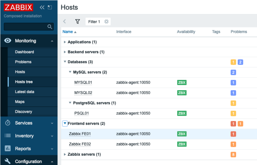
In this blog post, I’ll be using https://github.com/BGmot/zabbix-module-hosts-tree as an example which brings a brand new main menu element Monitoring -> Hosts tree showing the end-user a hierarchy of host groups instead of a flat list of hosts that comes with default Zabbix installation in Monitoring -> Hosts.

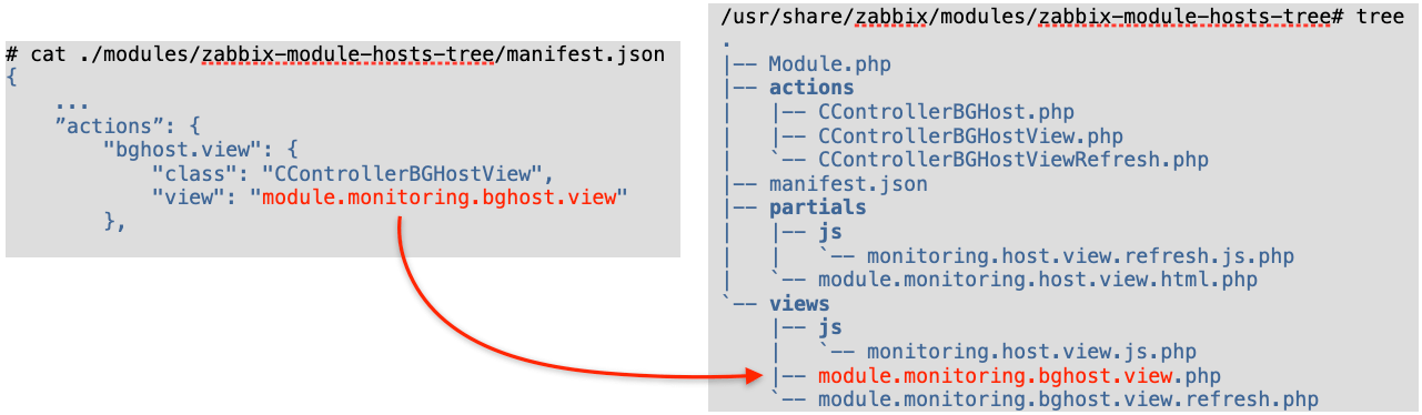
Refer to Zabbix official documentation on how to install modules and I won’t waste any time here on what is perfectly well documented. After this module is installed we’ll have the following files:

/usr/share/zabbix/modules/zabbix-module-hosts-tree# tree
.
|-- Module.php
|-- actions
| |-- CControllerBGHost.php
| |-- CControllerBGHostView.php
| `-- CControllerBGHostViewRefresh.php
|-- manifest.json
|-- partials
| |-- js
| | `-- monitoring.host.view.refresh.js.php
| `-- module.monitoring.host.view.html.php
`-- views
|-- js
| `-- monitoring.host.view.js.php
|-- module.monitoring.bghost.view.php
`-- module.monitoring.bghost.view.refresh.php

WebUI application

As mentioned earlier Zabbix WebUI is just a PHP application, yes, sophisticated, very complex but still it is a PHP application which means after every user click (and upon some timeouts), it initializes, executes and terminates producing some output (in most cases) which is passed to the user’s browser.

Top-level of this application is an object of class APP which inherits ZBase adding literally nothing, declared in file ./include/classes/core/APP.php:

class APP extends ZBase {
}

Application starts with ZBase::run() method, file ./include/config.inc.php:

APP::getInstance()->run(APP::EXEC_MODE_DEFAULT);

Method run() does many things, but in the light of this blog post it is important to mention these two:

  • router initialization
  • modules initialization

Router initialization

The so-called “Router” is a crucial part of the Controller component of MVC that drives a decision on how to handle a user’s request. The Router works based on an associative array $routes which is defined in ./include/classes/mvc/CRouter.php. Here is a code snippet illustrating how this array is organized:

private $routes = [
// action                   controller                        layout             view
‘action.operation.get'  => [‘CControllerActionOperationGet',  ‘layout.json',     null],
‘audit.settings.update' => [‘CControllerAuditSettingsUpdate',  null,             null],
‘dashboard.view'        => [‘CControllerDashboardView', ‘layout.htmlpage',   'monitoring.dashboard.view'],

As you can see in this array for every action three elements are defined:

  • controller (a class that will be used to prepare data)

  • layout (in which form to present data generated by the controller)

  • view (how to present/show the data to end-user/requestor)

We will talk about each of these components later. For now – just remember that the controller here is a class name while layout and view is a name of a .php file that is included (i.e. executed) at a certain point of webUI application execution. So Router Initialization is basically the class CRouter instantiation making $routes array available to other classes via CRouter‘s methods.

Modules initialization

This is the moment the web UI application goes through all enabled Modules in the system calling their init() method. Here in ZBase::run() methods init() are called and all the actions from enabled modules are added to the Router, file ./include/classes/core/ZBase.php:

$this->initModuleManager();
$router = $this->component_registry->get('router');
$router->addActions($this->module_manager->getActions());
$router->setAction($action_name);

Your module must be a child of Core\CModule class defined in ./include/classes/core/CModule.php. You can redefine init() method to fit your needs. Since init() method of all enabled Modules is called, this makes it a perfect place to have new menu items added to Zabbix WebUI main menu here.

We talked about Router in the previous clause and your module’s manifest.json file defines what needs to be added to this Router for your Module to function properly. If you defined an action in your Module that already exists in out-of-the-box Zabbix then the Module’s action overwrites the “default” entry in $router array thus, you can re-define the behavior of any menu item.

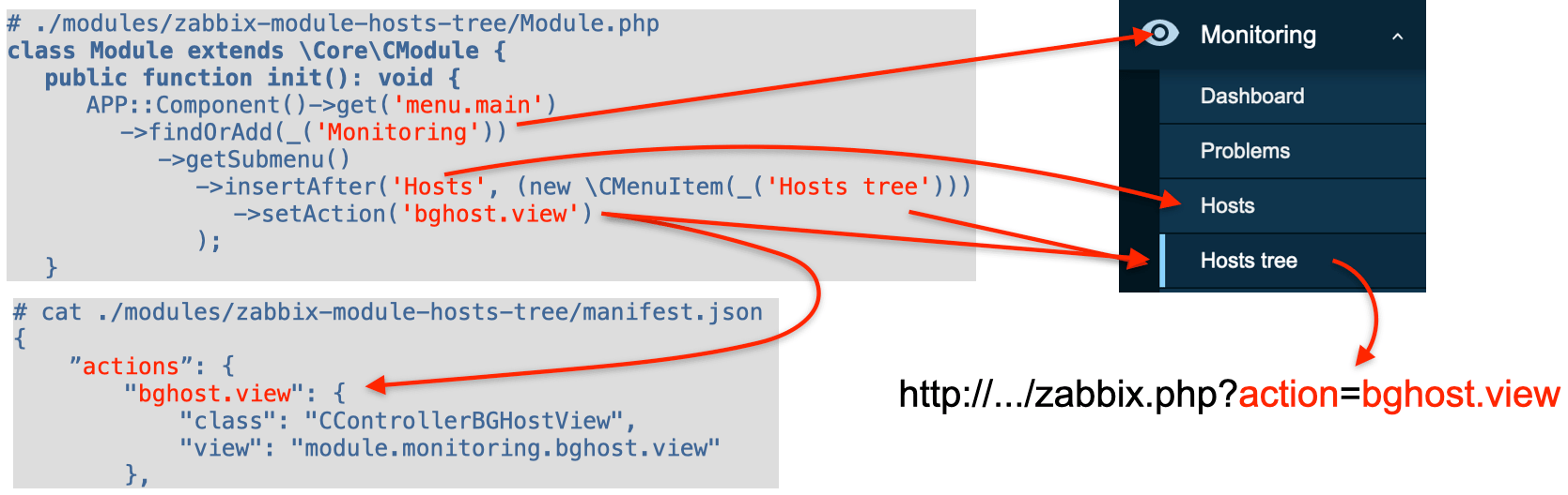
Overall what happens during the module initialization is easier to describe by following this picture:

So we added a new menu item “Hosts tree” under “Hosts” in the main menu. When a user clicks on this menu item a request will be generated with the parameter “action” set to “bghost.view” and now the Router “knows” that to serve this action it needs to use CControllerBGHostView class as a Controller and module.monitoring.bghost.view.php file (with default layout.html.php layout) to generate HTML code.

Processing request

After initialization is done the ZBase::processRequest() method is called, file ./include/classes/core/ZBase.php, passing initialized Router (let’s assume user selected Monitoring -> Hosts tree menu item implemented in my module):

$this->processRequest($router);
...
private function processRequest(CRouter $router): void {
  $action_name = $router->getAction();        // returns “bghost.view”
  $action_class = $router->getController();   // “Modules\BGmotHosts\Actions\CControllerBGHostView”
  ...
  $action = new $action_class();              // Controller defined for this action is instantiated
  ...
  register_shutdown_function(function() use ($action) {
    $this->module_manager->publishEvent($action, 'onTerminate');
  });

As we can see it gets the action name and action class name from the Router and then instantiates in variable $action a Controller class that will handle the requested action.

Then it registers all enabled modules onTerminate() methods – it means that before PHP execution exits all these functions will be executed regardless of what menu item a user selected. One important caveat: if a user selected an action covered by your module then your module’s onTerminate() method will be executed the last (later than all other modules’ onTerminate() methods) right when WebUI PHP application is about to finish its execution (i.e. exit). onTerminate() method of base class Core/CModule is empty and you can redefine it in your module, e.g., here is how I am adding my JavaScript to every page that generates HTML, ./modules/zabbix-module-menu/Module.php:

public function onTerminate(CAction $action): void {
  $action_page = $action->getAction();
  $router = clone APP::Component()->get('router');
  $layout = $router->getLayout();
  if ($action_page) {
    if ($action_page != 'jsrpc.php' &&
        $layout != 'layout.widget' &&
        $layout != 'layout.json') {
      echo '<script type="text/javascript">';
      echo file_get_contents(__DIR__.'/js/bg_menu.js');
      echo '</script>';
    }
  }
}

This approach works well only with layout.htmlpage layout as it just adds whatever you output here right before closing </body> tag in the final HTML page returned to browser.

Keep in mind we are still in ZBase::processRequest() method and now it executes all enabled modules’ onBeforeAction() methods:

$this->module_manager->publishEvent($action, 'onBeforeAction');

Again if a user selected an action covered by your module then your module’s onBeforeAction() method will be executed last. You can define onBeforeAction() method in your module this way:

public function onBeforeAction(CAction $action): void {
...
}

Processing request – Controller

Now ZBase::processRequest() passes execution to our Controller (remember $action was instantiated with our Controller class):

 $action->run();

All controllers have CController as a parent class. Method run() is defined in ./include/classes/mvc/CController.php and you cannot re-define it in your controller; it does some standards checks, validates input and if everything is ok passes control directly to your controller’s doAction() method and returns the result:

final public function run(): ?CControllerResponse {
  if ($this->checkInput()) {
    $this->doAction();
  return $this->getResponse();

Use your Controller’s checkInput() method to check whether all the parameters passed in the HTTP request are valid. You can implement it like this (see ./modules/zabbix-module-hosts-tree/actions/CControllerBGHostView.php):

 class CControllerBGHostView extends CControllerBGHost { 
        protected function checkInput(): bool {
                $fields = [             
                       'name' =>       'string',
                       'groupids' =>   'array_id',
                       'status' =>     'in -1,’.HOST_STATUS_MONITORED.','.HOST_STATUS_NOT_MONITORED,
                ...
                $ret = $this->validateInput($fields);
                return $ret;

All possible validation rules are defined in ./include/classes/validators/CNewValidator.php Just take a peek and select proper validation:

 # grep "case ‘" ./include/classes/validators/CNewValidator.php 
                                case ‘not_empty':
                                case 'json':
                                case ‘in':
                                ...
                                case 'array_id':
                                ...

If checkInput() method returns true (input is valid) then doAction() of your Controller is called. You can go as fancy as you want preparing data: executing internal Zabbix functions (The Model component of MVC), performing selects/updates in the database directly from your code, talk to other APIs, etc. At the end you need to prepare one massive associative array (usually it is named $data) and return it as shown here (./modules/zabbix-module-hosts-tree/actions/CControllerBGHostView.php):

 protected function doAction(): void {
     ...
     $data = [ ... ];
     $response = new CControllerResponseData($data);
     $response->setTitle(_('Hosts'));
     $this->setResponse($response);
 }

Whatever you place into the associative array $data will be available later in your View code.

Processing request – View

The final step in ZBase::processRequest() is calling one more method that in fact handles the layout and view you defined in the Router for this action:

$this->processResponseFinal($router, $action);

The name of your view file is what you put into the view field for your action in manifest.json + .php extension and must be in the views/ folder.

First, it fills in the layout data with defaults and if a view is defined for given action then it constructs an instance of CView class (defined in ./include/classes/mvc/CView.php) passing data you prepared in Controller to CView constructor:

private function processResponseFinal(CRouter $router, CAction $action): void {
  ...
  if ($router->getView() !== null && $response->isViewEnabled()) {
    $view = new CView($router->getView(), $response->getData());

CView constructor just tries to find a file with the name of your View + .php extension, e.g. module.monitoring.bghost.view.php and, if found, initializes two member variables $name and $data.

public function __construct($name, array $data = []) {

Everything you implement in your View .php file will feed the $layout_data variable.

$layout_data = array_replace($layout_data_defaults, [
  'main_block' => $view->getOutput(),
  'javascript' => [ 'files' => $view->getJsFiles() ],
  'stylesheet' => [ 'files' => $view->getCssFiles() ],
  'web_layout_mode' => $view->getLayoutMode()
]);

CView::getOutput() simply performs PHP include of your view .php file, so whatever you “print” in your view will be assigned to $layout_data[‘main_block’], file ./include/classes/mvc/CView.php:

public function getOutput() {
  $file_path = $this->directory.’/'.$this->name.'.php';
  ob_start();
  if ((include $file_path) === false) {
    ...
  return ob_get_clean();

If you have a lot of time and want to produce a real “piece of art” web page then you can print pure HTML/CSS in your view .php file, but it will most probably not look like the “Zabbix native style”. For example:

Fortunately, there is an easy solution to make your web pages look elegant and totally “Zabbix’ish”: it is very easy to use Zabbix classes, e.g., to add a table to your page use CTableInfo class, then prepare an array with CColHeader elements and add them with CTableInfo::setHeader(), then construct rows with CRow class and add them via CTableInfo::addRow(), etc.

Look at the Zabbix source code for an example of how to use them.
 See the list of all out-of-the-box classes here:

# ls -1 ./include/classes/html/
CActionButtonList.php
CBarGauge.php
CButton.php
...

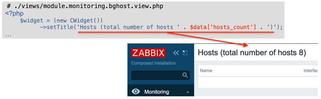
Since we passed all the data generated by your Controller to your View object, it is very easy to use the data in your View code, e.g., in Controller you do the following:

 # ./modules/zabbix-module-hosts-tree/actions/CControllerBGHostView.php
 protected function doAction(): void {
     $data = [ 'hosts_count' => API::Host()->get(['countOutput' => true]) ];
     $response = new CControllerResponseData($data);
     $this->setResponse($response);
 }

And in View you use this data:

If you want to add some CSS files to the page, do it in your View code this way:

 # ./views/module.monitoring.bghost.view.php
 $this->addCssFile('modules/zabbix-module-hosts-tree/views/css/mycool.css');

Your CSS file should not contain <style> tags, just pure CSS:

 # ./views/css/mycool.css
 .list-table thead th {color: #ff0000;}

Interestingly enough you cannot add JavaScript files from your module folder using a similar addJsFile() method. You can use this method only to use the JS files that come with Zabbix and are located in the root /js folder, e.g.:

 # ./views/module.monitoring.bghost.view.php
 $this->addJsFile('multiselect.js');

To include your JavaScript code use this function. Note this .php file that must have PHP code that by “printing” generates JavaScript code, not .js (containing pure JavaScript code).

 # ./views/module.monitoring.bghost.view.php
 $this->includeJsFile('monitoring.host.view.js.php', $data);

– Again: this .php file must “print” JavaScript code and will be searched in the ./js
 subfolder of the view file this function is invoked from.
– A copy of $data variable will be available for use within the file!

So all the HTML code you generated went into $layout_data[‘main_block’], all JavaScript files that need to be included went into $layout_data[‘javascript’] and all CSS files that need to be included went into $layout_data[‘stylesheet’] (see $layout_data variable initialization above in this article).

The last thing ZBase::processResponseFinal() does is instantiate the new CView class with a layout .php file (you define the layout for every action in Router, remember?) and “printing” everything according to the selected layout, file ./include/classes/core/ZBase.php:

echo (new CView($router->getLayout(), $layout_data))->getOutput();

That is it! At this point, everything you “printed” (don’t forget the onTerminate() function) is returned as an HTTP response to the user’s browser.

Wrapping up this article I must tell you about one more thing – module configuration. In your modules’ manifest.json file you can have a “config” section –  below you can see how it is reflected in the Zabbix database:

I would not mention this, but there is one interesting caveat: the “config” section of manifest.json file is copied into the database only when the module is discovered for the first time during modules directory scanning. Changing the manifest.json file later has no effect; module’s config is always taken from the database so if you want to change something you either need to first wipe the module or make changes directly in the database.
Access this config data in your code with $this->getConfig();

Good luck developing Web Modules!
Your BGmot.

Three new winners of Project Jengo, and more defeats for the patent troll

Post Syndicated from Ethan Park original https://blog.cloudflare.com/three-new-winners-of-project-jengo-and-more-defeats-for-the-patent-troll/

Three new winners of Project Jengo, and more defeats for the patent troll

Three new winners of Project Jengo, and more defeats for the patent troll

Project Jengo is a Cloudflare effort to fight back against patent trolls by flipping the incentive structure that has encouraged the growth of patent trolls who extract settlements out of companies using frivolous lawsuits. We do this by asking the public to identify prior art that can invalidate any of the patents that a troll holds – not just the ones that are asserted against Cloudflare.

Since we launched Project Jengo over five years ago, we’ve given out over $135,000 to individuals who helped us find prior art to invalidate patents owned by patent trolls. By invalidating those patents – many of which are so blatantly marginal or broad that they never should have been granted in the first place – we hope to decrease the amount of harassment and frivolous lawsuits that patent trolls bring against innovative technology companies.

Today, we’re excited to announce three new Project Jengo winners. These individuals have helped us push forward our effort to take down patent trolls, and continue to fight trolling in favor of innovation.

The patent troll

The current case involves a patent troll called Sable Networks who asserted four patents that generally describe a flow-based router or a mechanism for identifying and penalizing misbehaving flows against Cloudflare. We’ve implemented Project Jengo against Sable on those four patents and their six other patents, which they haven’t asserted against Cloudflare. Today’s recipients have helped us in that fight.

And we continue to fight Sable Networks before the Court and the U.S. Patent Office as well. We have a major case update in that regard as the U.S. Patent Office agreed that most of the claims from Sable’s ’593 patent should have never been issued in the first place, which means Sable is down to two patents in their lawsuit against Cloudflare. More on that later, but first, here are the three winners from Chapters 4, 5, and 6 of Project Jengo!

Chris Wheeler from Georgia, who has a patent of his own

We are excited to announce Chris Wheeler as the winner of the 4th chapter of Project Jengo! Chris is the CTO and a co-founder of a software startup in Macon, Georgia called Tier2 Technologies, and he is now $5,000 richer!

When we asked where he had heard about Project Jengo, Chris told us:

“I heard about Project Jengo from one of your blog posts. I often read your blog on my phone from my children’s bedroom at night while I’m waiting for them to fall asleep. I’m a huge fan of Cloudflare and use your services myself extensively.”

As for why he submitted, Chris holds a patent, and submitted to Project Jengo in part because he was “drawn to the idea of helping protect the integrity of the patent system.”

Chris submitted a paper titled “A Framework for Alternate Queueing: Towards Traffic Management by PC-UNIX Based Routers” as prior art to Sable’s ’932 patent. This paper was published in 1998. On the other hand, Sable’s ’932 patent was filed in 2002 and is alleged to cover routers utilizing aggregate flow blocks that include tunnel-specific information for selected network paths. The aggregate flow blocks are also alleged to store statistics pertaining to the selected network paths. This paper, published nearly four years prior to the filing of the ’932 patent, describes a PC-UNIX based router that implements a FreeBSD Alternate Queueing (ALTQ) driver with traffic management functionalities to select network paths. ALTQ traffic management uses queueing disciplines based on stored statistical analysis of selected paths for network traffic, and this is a great prior art reference to the ’932 patent.

His breakdown of his submission is interesting too:

“When I saw the claims in 6,977,932 I immediately thought ‘They are just describing QoS in a weird convoluted way’ and I knew QoS had existed long before the patent date of 2002. I have used the ALTQ packet scheduler in pfSense a lot in the past throughout my career, and that was the first thing that came to my mind. I did a quick Google search for ‘ALTQ’ and found the oldest reference I could find, which was from 1998.”

We appreciate his efforts, as he managed to find useful prior art from four years before the patent in question. Thank you, Chris!

Peter’s first foray into patent law makes him $5,000 richer!

Additionally, we are awarding $5,000 to Peter S. for finding us a valuable thesis paper! This is Peter’s first foray into patent law, and we are so thankful for his time and effort.​​

The thesis of Rena Whei-Ming Yang found by Peter describes the solution of the ʼ593 patent almost five years before Sable even filed for the patent! The ʼ593 patent is the Sable patent concerning the detection of “bad” flows. Yang—years before Sable—developed the same thing: “This thesis studies a means of using such mechanisms to identify nonadaptive network flows, and proposes a protocol to push this information, along with penalization responsibility, towards the flows’ sources.” What Sable calls “bad,” Yang labels “nonadaptive.” The important thing is that Yang’s work predates the ’593 patent’s alleged new solutions by years, making it a great find. Thank you, Peter!

David who hopes the Patent Office will adopt new technologies for better examinations

Finally, we are excited to announce the winner from the 6th Chapter of Project Jengo, and that is David H. who is receiving a $5,000 prize! David’s background is in accounting/finance, but became interested in patents and IP back in 2010. He heard about Project Jengo through a LinkedIn post and thought it was an excellent idea, so he put his search skills to task.

David identified U.S. Patent No. 6,859,438 for us, which is a patent entitled “Policy Based Quality of Service.” This ’438 patent discloses the same “quality of service” (or QoS) technology claimed in Sable’s ’431 patent, with one important difference: the disclosure of the ’438 patent dates back to an application filed on February 3, 1998, but the disclosure in the ’431 patent wasn’t filed until (at the earliest), April 19, 2000. So the technology explained in the ’438 patent—a flexible, policy-based, mechanism for managing, monitoring, and prioritizing traffic within a network and allocating bandwidth to achieve true QoS—beat Sable to the punch on the “new” switching technology claimed in the ’431 patent that purports to provide a previously “unavailable” degree of quality of service, by more than two years! Excellent find, David!

He also shared his thoughts on the current state of the U.S. patent system:

“The US Patent Office continues to issue patents that are likely invalid on a number of grounds with a large proportion to big tech. The USPTO has a nice fee generating business, being able to get paid issuing patents and subsequently canceling them in post grant proceedings. I am hopeful the USPTO adopts new technology to aid examiners in their prosecution efforts.”

Thank you, David!

* * *

Congratulations and our deep gratitude to all three winners from Chapters 4-6 of Project Jengo. Remember, we have committed \$100,000 to this prior art search, and we still have $50,000 to give out! The search is still ongoing, so please help us beat the patent troll by submitting prior art references here. The submission deadline for Chapter 7 is January 31, 2023, so don’t delay your search!

Three new winners of Project Jengo, and more defeats for the patent troll

Case updates: Another patent thrown out of the case, and the few remaining claims further whittled down

When Sable sued us almost two years ago in March 2021, they accused us of infringing four different patents, which included a total of 134 claims. We previously shared how we successfully killed off one of the four patents, known as the ’932 patent.

Today, we have more great news to share. The U.S. Patent Office agreed with us that all the claims from the ’593 patent that Sable asserted against us are invalid. This means we were able to get yet another patent – the ’593 patent – dropped out of Sable’s case against us.

A single U.S. patent usually has somewhere around 10 to 20 claims (here’s a Wiki page explaining what a “claim” is in patents), but Sable’s ’593 patent included a whopping number of claims – 44 to be exact. As we previously shared back in January 2022, the Patent Office ruled that we would likely be successful in invalidating all 44 claims of the ’593 patent and instituted a trial proceeding known as inter partes review (IPR). Since then, Sable voluntarily canceled 17 of the claims – presumably because they themselves knew those claims were invalid. Of the remaining 27 claims, the Patent Office determined that 23 claims were invalid. Because none of the four surviving claims – which escaped invalidation only by virtue of a procedural technicality – are part of Sable’s case against us, the ’593 patent is no longer asserted against us. And given the record we have established before the Patent Office, we don’t think Sable will try asserting those four surviving claims from the ’593 patent against any of our peer companies. But even if Sable does, they should be able to leverage what we’ve done and kill off the patent completely.

Our victory was covered by multiple legal news outlets such as Bloomberg Law and Law360 (unfortunately, subscription required). A special shoutout to our attorney Jim Day of Farella Braun + Martel, who fought hard to get rid of these toxic claims that should have never been issued! With two patents completely out of the case, there are now only two patents at issue in Sable’s case against us.

We have even more good news to share! In October 2022, the Court found nine claims from one of the two remaining patents – the ’431 patent – to be invalid for failure to meet certain statutory requirements. This means Sable only has 14 claims from two patents in the case. Considering that we started this journey with Sable asserting 131 claims from four patents against us, we are proud of what we have accomplished thus far. We successfully persuaded the Court and the Patent Office to cancel, or forced Sable to voluntarily cancel, almost 90% of those 131 claims. Those victories not only help us in our case against Sable, they will also protect all innovative companies from being accused frivolously of infringing those invalid claims.

Our trial is scheduled for November 2023, but we will have more updates for you before then. Stay tuned, and remember to go look for prior art references to help us in our fight against this patent troll!

Three new winners of Project Jengo, and more defeats for the patent troll

The FBI Identified a Tor User

Post Syndicated from Bruce Schneier original https://www.schneier.com/blog/archives/2023/01/the-fbi-identified-a-tor-user.html

No details, though:

According to the complaint against him, Al-Azhari allegedly visited a dark web site that hosts “unofficial propaganda and photographs related to ISIS” multiple times on May 14, 2019. In virtue of being a dark web site—­that is, one hosted on the Tor anonymity network—­it should have been difficult for the site owner’s or a third party to determine the real IP address of any of the site’s visitors.

Yet, that’s exactly what the FBI did. It found Al-Azhari allegedly visited the site from an IP address associated with Al-Azhari’s grandmother’s house in Riverside, California. The FBI also found what specific pages Al-Azhari visited, including a section on donating Bitcoin; another focused on military operations conducted by ISIS fighters in Iraq, Syria, and Nigeria; and another page that provided links to material from ISIS’s media arm. Without the FBI deploying some form of surveillance technique, or Al-Azhari using another method to visit the site which exposed their IP address, this should not have been possible.

There are lots of ways to de-anonymize Tor users. Someone at the NSA gave a presentation on this ten years ago. (I wrote about it for the Guardian in 2013, an essay that reads so dated in light of what we’ve learned since then.) It’s unlikely that the FBI uses the same sorts of broad surveillance techniques that the NSA does, but it’s certainly possible that the NSA did the surveillance and passed the information to the FBI.

How to encrypt sensitive caller voice input in Amazon Lex

Post Syndicated from Herbert Guerrero original https://aws.amazon.com/blogs/security/how-to-encrypt-sensitive-caller-authentication-voice-input-in-amazon-lex/

In the telecommunications industry, sensitive authentication and user data are typically received through mobile voice and keypads, and companies are responsible for protecting the data obtained through these channels. The increasing use of voice-driven interactive voice response (IVR) has resulted in a need to provide solutions that can protect user data that is gathered from mobile voice inputs. In this blog post, you’ll see how to protect a caller’s sensitive voice data that was captured through Amazon Lex by using data encryption implemented through AWS Lambda functions. The solution described in this post helps you to protect customer data received through voice channels from inadvertent or unknown access. The solution also includes decryption capabilities, which give an authorized administrator or operator the ability to decrypt user data from a Lambda console.

Solution overview

To demonstrate the IVR solution described in this post, a caller speaks two sensitive pieces of data—credit card number and zip code—from an Amazon Connect contact flow. The spoken values are encrypted and returned to the contact flow to be stored in contact attributes. The encrypted ciphertext is retained as a contact attribute for decryption purposes. Amazon CloudWatch Logs is enabled in the contact flow, but only the encrypted values are logged in log streams.

For this solution, conversation logs for this Amazon Lex bot are not enabled. An operator with assigned AWS Identity and Access Management (IAM) permissions can monitor the logged encrypted entries from CloudWatch Logs. For more information, see Working with log groups and log streams in the Amazon CloudWatch Logs User Guide.

Solution architecture

Figure 1 shows the overview of the solution described in this blog post.

Figure 1: Example of solution architecture

Figure 1: Example of solution architecture

Figure 1 shows the following high-level steps of the solution, and the number labels correspond to the following steps.

  1. A caller places an inbound call.
  2. An Amazon Connect contact flow leverages a Get customer input block, backed by an Amazon Lex bot, to prompt the caller for numerical data.
  3. The Amazon Lex bot invokes the Lambda function dev-encryption-core-EncryptFn.
  4. The Lambda function uses the AWS Encryption SDK to encrypt the caller’s plain text data.
  5. The AWS Encryption SDK obtains encryption keys from AWS Key Management Service (AWS KMS).
  6. The caller’s data is encrypted by using the AWS KMS keys obtained from AWS KMS.
  7. The Lambda function appends the encrypted data to the Amazon Lex bot session attributes.
  8. Amazon Lex returns the fully encrypted data back to Amazon Connect.

Overview of a contact flow

Figure 2: Contact flow captures input values using Amazon Lex and returns their encrypted values

Figure 2: Contact flow captures input values using Amazon Lex and returns their encrypted values

Figure 2 shows an overview of the contact flow, which has two main steps:

  1. The first numerical data (in this example, an encrypted credit card number value) is stored in contact attributes.
  2. The second numerical data (in this example, an encrypted zip code value) is stored in contact attributes.

Prerequisites

This solution uses the following AWS services:

The following need to be installed in your local machine:

To implement the solution in this post, you first need the Amazon Connect instance prerequisite in place.

To set up the Amazon Connect instance (if none exists)

  1. Create an Amazon Connect instance with a claimed phone number and a configured Amazon Connect user linked to a basic routing profile. For more information about setting up a contact center, see Set up your contact center in the Amazon Connect Administrator Guide.
  2. Assign the CallCenterManager or Admin security profile to an Amazon Connect user.
  3. In the newly created Amazon Connect instance, under the Overview section, find the access URL with the format
    https://<aliasname>.awsapps.com/connect/login

    • Make note of the access URL, which you will use later to log in to the Amazon Connect Dashboard.
  4. Log in to your Amazon Connect instance with a Connect user that has Admin or CallCenterManager permissions.

Solution procedures

This solution includes the following procedures:

  1. Clone the project or download the solution zip file.
  2. Create AWS resources needed for encryption and decryption.
  3. Configure the Amazon Lex bot in Amazon Connect.
  4. Create the contact flow in Amazon Connect.
  5. Validate the solution.
  6. Decrypt the collected data.

To clone or download the solution

  • Log in to the GitHub repo.
  • Clone or download the solution files to your local machine.

The downloaded file contains the artifacts needed for the deployment.

To create AWS resources needed for encryption and decryption

  1. From the command line, change directory to the project’s root directory.
  2. Run npm install.
  3. Run npm run build to transpile TypeScript to JavaScript and package code and its dependencies before deploying to AWS.
  4. Run cdk deploy CoreStack.

To configure the Amazon Lex bot in your Amazon Connect instance

  1. In the Amazon Connect console, choose Contact flows and scroll to the Amazon Lex section.
    Figure 3: Select Contact flows

    Figure 3: Select Contact flows

  2. From the Bot menu, select secure_LexInput(Classic). Then select +Add Amazon Lex Bot.
    Figure 4: Configure the Amazon Lex bot to Amazon Connect

    Figure 4: Configure the Amazon Lex bot to Amazon Connect

To import contact flow into Amazon Connect

  1. In the Amazon Connect console, choose Overview, and then choose Login as administrator.
  2. From the Routing menu on the left side, choose Contact flows to show the list of contact flows.
  3. Choose Create Contact flow.
  4. Choose the arrow to the right of the Save button and choose Import flow (beta). This imports the contact flow that you previously downloaded in the procedure To clone or download the solution.

    The contact flow already has the Amazon Lex bot configured.

    Figure 5: Select Import flow (beta)

    Figure 5: Select Import flow (beta)

  5. In the upper right corner of the contact flow, choose Save, and then choose OK to save the changes.
  6. Choose Publish to make the contact flow ready for use during the validation steps.
  7. (Optional) Claim a phone number (if none is available), using the following steps:
    1. In the Connect Dashboard, on the navigation menu, choose Channels, and then choose Phone numbers.
    2. On the right side of the page, choose Claim a number.
    3. Select the DID (Direct Inward Dialing) tab. Use the drop-down arrow to choose your country/region. When numbers are returned, choose one.
    4. Write down the phone number. You call it later in this post.
  8. (Optional) On the Edit Phone number page, in the Description box, you can type a note if desired.
  9. To assign the contact flow to your claimed phone number, for Contact flow / IVR, choose the drop-down arrow, and then choose Secure_Lex_Input.
  10. Choose Save.
    Figure 6: Under Contact flow / IVR, select the imported contact flow

    Figure 6: Under Contact flow / IVR, select the imported contact flow

For more information, see Set up phone numbers for your contact center in the Amazon Connect Administrator Guide.

To validate the solution

  1. Dial the test phone number to go through the voice prompt flow.
  2. When prompted, speak a 16-digit credit card number (you have a maximum of two retries), then speak a 5-digit zip code (also a maximum of two retries).
  3. After you complete your test call, review the log streams in Amazon CloudWatch Logs to confirm that the digits that you entered are now encrypted and stored as a contact attribute. The two entered values zipcode and creditcard are stored in contact attributes. Both are encrypted.
    Figure 7: Sample log showing encrypted values for zipcode and creditcard

    Figure 7: Sample log showing encrypted values for zipcode and creditcard

  4. Log in to your Amazon Connect Dashboard as a Supervisor. The URL is provided after the connect instance has been created. In the navigation menu, choose Contact search.
    Figure 8: Choose Contact search to look for the call information

    Figure 8: Choose Contact search to look for the call information

  5. Locate your inbound call on the Contact search list. Note that it can take up to 60 seconds for data to appear in the Contact search list.
  6. Select the Contact ID for your call.
    Figure 9: The Contact search showing the contact details for your test call

    Figure 9: The Contact search showing the contact details for your test call

  7. Copy the encrypted values for creditcard and zipcode and make note of them; you will use these values in the next procedure.
    Figure 10: Contact attributes stored in a contact flow are registered as part of the contact details

    Figure 10: Contact attributes stored in a contact flow are registered as part of the contact details

To decrypt the collected data

  1. In the AWS Lambda console, choose Functions.
  2. Use the Search bar to look for the dev-encryption-core-DecryptFn Lambda function, and then select the name link to open it.
  3. Under folder encryption-master, open the test folder. Under the tab \events, locate the file decrypt.json.
  4. Use the following steps to create a sample test event in the console by using the contents from decrypt.json. For more details, see Testing Lambda functions in the console.
    1. Choose the down arrow on the right side of Test.
    2. Choose Configure test event.
    3. Choose Create new test event.
    4. For Event name, enter decryptTest.
    5. Paste the contents from decrypt.json.
      {
          "Details": {
              "Parameters": {
                  "encrypted": "<encrypted-value-here>"
              }
          }
      }

    6. Choose Save.
  5. Use the encrypted values saved in the Validate a solution procedure and replace the ones in the recently created test event.
    Figure 11: Replace the creditcard or zipCode values with the ones from the Contact Search page

    Figure 11: Replace the creditcard or zipCode values with the ones from the Contact Search page

  6. Choose Test. The output from the test shows the values decrypted by the Lambda function. This is shown in Figure 12 under the Execution result tab.
    Figure 12: Result from the decryption operation

    Figure 12: Result from the decryption operation

Note: Make sure that only the appropriate authorized administrator or operator, application, or AWS service is able to invoke the decryption Lambda function.

You have now successfully implemented the solution by encrypting and decrypting the voice input of your test call, which you collected through Amazon Lex.

Cleanup

To avoid incurring future charges, follow these steps to clean up the deployed resources that you created when implementing this solution.

To delete the Amazon Connect instance

  1. In the Amazon Connect console, under Instance alias, select the name of the Amazon Connect instance, and choose Delete.
  2. When prompted, type the name of the instance, and then choose Delete.

To delete the Amazon Lex bot

  1. In the Amazon Lex console, choose the bot that you created in the To configure the Amazon Lex bot procedure.
  2. Choose Delete, and then choose Continue.

To delete the AWS CloudFormation stack

  1. In the AWS CloudFormation console, on the Stacks page, select the stack you created in the procedure To create AWS resources needed for encryption and decryption.
  2. In the stack details pane, choose Delete.
  3. Choose Delete stack when prompted. This deletes the Amazon S3 bucket, IAM roles and AWS Lambda functions you created for testing. This will also schedule a deletion date on the AWS KMS key.

Conclusion

In this post, you learned how an Amazon Connect contact flow can collect voice inputs from a caller by using Amazon Lex, and how you can encrypt these inputs by using your own AWS KMS key. This solution can help improve the security of voice input that is collected through Amazon Connect. For cost information, see the Amazon Connect pricing page.

For more information, see the blog post Creating a secure IVR solution with Amazon Connect and the topic Encrypt customer input (using OpenSSL) in the Amazon Connect Administrator Guide. As previously mentioned, the increasing use of voice-driven IVR has resulted in a need to provide solutions that can protect user data gathered from mobile voice inputs.

Additional resources include the AWS Lambda Developer Guide, the Amazon Lex Developer Guide, the Amazon Connect Administrator Guide, the AWS Nodejs SDK, and the AWS SDK for Python (Boto3).

If you need help with setting up this solution, you can get assistance from AWS Professional Services. You can also seek assistance from Amazon Connect partners available worldwide.

 
If you have feedback about this post, submit comments in the Comments section below. If you have questions about this post, contact AWS Support.

Want more AWS Security news? Follow us on Twitter.

Herbert Guerrero

Herbert Guerrero

Herbert is a Senior Proserve Consultant for Connect. He enjoys designing and developing high-usability and scalable solutions. Understanding success criteria helps Herbert work backwards and deliver well-architected solutions. His engineering background informs the way he engages with customers’ mental models of what their solutions should look like.

Ed Valdez

Ed Valdez

Ed is a Specialty Consultant with Amazon Web Services. As a software development professional with over 23 years of experience, he specializes on designing and delivering customer-centric solutions within the contact center domain.

AWS Week in Review – January 16, 2023

Post Syndicated from Antje Barth original https://aws.amazon.com/blogs/aws/aws-week-in-review-january-16-2023/

Today, we celebrate Martin Luther King Jr. Day in the US to honor the late civil rights leader’s life, legacy, and achievements. In this article, Amazon employees share what MLK Day means to them and how diversity makes us stronger.

Coming back to our AWS Week in Review—it’s been a busy week!

Last Week’s Launches
Here are some launches that got my attention during the previous week:

AWS Local Zones in Perth and Santiago now generally available – AWS Local Zones help you run latency-sensitive applications closer to end users. AWS now has a total of 29 Local Zones; 12 outside of the US (Bangkok, Buenos Aires, Copenhagen, Delhi, Hamburg, Helsinki, Kolkata, Muscat, Perth, Santiago, Taipei, and Warsaw) and 17 in the US. See the full list of available and announced AWS Local Zones and learn how to get started.

AWS Local Zones Locations

AWS Clean Rooms now available in preview – During AWS re:Invent this past November, we announced AWS Clean Rooms, a new analytics service that helps companies across industries easily and securely analyze and collaborate on their combined datasets—without sharing or revealing underlying data. You can now start using AWS Clean Rooms (Preview).

Amazon Kendra updates – Amazon Kendra is an intelligent search service powered by machine learning (ML) that helps you search across different content repositories with built-in connectors. With the new Amazon Kendra Intelligent Ranking for self-managed OpenSearch, you can now improve the quality of your OpenSearch search results using Amazon Kendra’s ML-powered semantic ranking technology.

Amazon Kendra also released an Amazon S3 connector with VPC support to index and search documents from Amazon S3 hosted in your VPC, a new Google Drive Connector to index and search documents from Google Drive, a Microsoft Teams Connector to enable Microsoft Teams messaging search, and a Microsoft Exchange Connector to enable email-messaging search.

Amazon Personalize updates – Amazon Personalize helps you improve customer engagement through personalized product and content recommendations. Using the new Trending-Now recipe, you can now generate recommendations for items that are rapidly becoming more popular with your users. Amazon Personalize now also supports tag-based resource authorization. Tags are labels in the form of key-value pairs that can be attached to individual Amazon Personalize resources to manage resources or allocate costs.

Amazon SageMaker Canvas now delivers up to 3x faster ML model training time – SageMaker Canvas is a visual interface that enables business analysts to generate accurate ML predictions on their own—without having to write a single line of code. The accelerated model training times help you prototype and experiment more rapidly, shortening the time to generate predictions and turn data into valuable insights.

For a full list of AWS announcements, be sure to keep an eye on the What’s New at AWS page.

Other AWS News
Here are some additional news items and blog posts that you may find interesting:

AWS open-source news and updates – My colleague Ricardo writes this weekly open-source newsletter in which he highlights new open-source projects, tools, and demos from the AWS Community. Read edition #141 here.

ML model hosting best practices in Amazon SageMaker – This seven-part blog series discusses best practices for ML model hosting in SageMaker to help you identify which hosting design pattern meets your needs best. The blog series also covers advanced concepts such as multi-model endpoints (MME), multi-container endpoints (MCE), serial inference pipelines, and model ensembles. Read part one here.

I would also like to recommend this really interesting Amazon Science article about differential privacy for end-to-end speech recognition. The data used to train AI models is protected by differential privacy (DP), which adds noise during training. In this article, Amazon researchers show how ensembles of teacher models can meet DP constraints while reducing error by more than 26 percent relative to standard DP methods.

Upcoming AWS Events
Check your calendars and sign up for these AWS events:

#BuildOnLive – Build On AWS Live events are a series of technical streams on twitch.tv/aws that focus on technology topics related to challenges hands-on practitioners face today.

  • Join the Build On Live Weekly show about the cloud, the community, the code, and everything in between, hosted by AWS Developer Advocates. The show streams every Thursday at 09:00 US PT on twitch.tv/aws.
  • Join the new The Big Dev Theory show, co-hosted with AWS partners, discussing various topics such as data and AI, AIOps, integration, and security. The show streams every Tuesday at 08:00 US PT on twitch.tv/aws.

Check the AWS Twitch schedule for all shows.

AWS Community Days – AWS Community Day events are community-led conferences that deliver a peer-to-peer learning experience, providing developers with a venue to acquire AWS knowledge in their preferred way: from one another.

AWS Innovate Data and AI/ML edition – AWS Innovate is a free online event to learn the latest from AWS experts and get step-by-step guidance on using AI/ML to drive fast, efficient, and measurable results.

  • AWS Innovate Data and AI/ML edition for Asia Pacific and Japan is taking place on February 22, 2023. Register here.
  • Registrations for AWS Innovate EMEA (March 9, 2023) and the Americas (March 14, 2023) will open soon. Check the AWS Innovate page for updates.

You can browse all upcoming in-person and virtual events.

That’s all for this week. Check back next Monday for another Week in Review!

— Antje

This post is part of our Week in Review series. Check back each week for a quick roundup of interesting news and announcements from AWS!

How to revoke federated users’ active AWS sessions

Post Syndicated from Matt Howard original https://aws.amazon.com/blogs/security/how-to-revoke-federated-users-active-aws-sessions/

When you use a centralized identity provider (IdP) for human user access, changes that an identity administrator makes to a user within the IdP won’t invalidate the user’s existing active Amazon Web Services (AWS) sessions. This is due to the nature of session durations that are configured on assumed roles. This situation presents a challenge for identity administrators.

In this post, you’ll learn how to revoke access to specific users’ sessions on AWS assumed roles through the use of AWS Identity and Access Management (IAM) policies and service control policies (SCPs) via AWS Organizations.

Session duration overview

When you configure IAM roles, you have the option of configuring a maximum session duration that specifies how long a session is valid. By default, the temporary credentials provided to the user will last for one hour, but you can change this to a value of up to 12 hours.

When a user assumes a role in AWS by using their IdP credentials, that role’s credentials will remain valid for the length of their session duration. It’s convenient for end users to have a maximum session duration set to 12 hours, because this prevents their sessions from frequently timing out and then requiring re-login. However, a longer session duration also poses a challenge if you, as an identity administrator, attempt to revoke or modify a user’s access to AWS from your IdP.

For example, user John Doe is leaving the company and you want to verify that John has his privileges within AWS revoked. If John has access to IAM roles with long-session durations, then he might have residual access to AWS despite having his session revoked or his user identity deleted within the IdP. Perhaps John assumed a role for his daily work at 8 AM and then you revoked his credentials within the IdP at 9 AM. Because John had already assumed an AWS role, he would still have access to AWS through that role for the duration of the configured session, 8 PM if the session was configured for 12 hours. Therefore, as a security best practice, AWS recommends that you do not set the session duration length longer than is needed. This example is displayed in Figure 1.

Figure 1: Session duration overview

Figure 1: Session duration overview

In order to restrict access despite the session duration being active, you could update the roles that are assumable from an IdP with a deny-all policy or delete the role entirely. However, this is a disruptive action for the users that have access to this role. If the role was deleted or the policy was updated to deny all, then users would no longer be able to assume the role or access their AWS environment. Instead, the recommended approach is to revoke access based on the specific user’s principalId or sourceIdentity values.

The principalId is the unique identifier for the entity that made the API call. When requests are made with temporary credentials, such as assumed roles through IdPs, this value also includes the session name, such as [email protected]. The sourceIdentity identifies the original user identity that is making the request, such as a user who is authenticated through SAML federation from an IdP. As a best practice, AWS recommends that you configure this value within the IdP, because this improves traceability for user sessions within AWS. You can find more information on this functionality in the blog post, How to integrate AWS STS SourceIdentity with your identity provider.

Identify the principalId and sourceIdentity by using CloudTrail

You can use AWS CloudTrail to review the actions taken by a user, role, or AWS service that are recorded as events. In the following procedure, you will use CloudTrail to identify the principalId and sourceIdentity contained in the CloudTrail record contents for your IdP assumed role.

To identify the principalId and sourceIdentity by using CloudTrail

  1. Assume a role in AWS by signing in through your IdP.
  2. Perform an action such as a creating an S3 bucket.
  3. Navigate to the CloudTrail service.
  4. In the navigation pane, choose Event History.
  5. For Lookup attributes, choose Event name. For Event name, enter CreateBucket.
  6. Figure 2: Looking up the CreateBucket event in the CloudTrail event history

    Figure 2: Looking up the CreateBucket event in the CloudTrail event history

  7. Select the corresponding event record and review the event details. An example showing the userIdentity element is as follows.

"userIdentity": {
	"type": "AssumedRole",
	"principalId": 
"AROATVGBKRLCHXEXAMPLE:[email protected]",
	"arn": "arn:aws:sts::111122223333:assumed-
role/roleexample/[email protected]",
	"accountId": "111122223333",
	"accessKeyId": "ASIATVGBKRLCJEXAMPLE",
	"sessionContext": {
		"sessionIssuer": {
			"type": "Role",
			"principalId": "AROATVGBKRLCHXEXAMPLE",
			"arn": 
"arn:aws:iam::111122223333:role/roleexample",
			"accountId": "111122223333",
			"userName": "roleexample"
		},
		"webIdFederationData": {},
		"attributes": {
			"creationDate": "2022-07-05T15:48:28Z",
			"mfaAuthenticated": "false"
		},
		"sourceIdentity": "[email protected]"
	}
}

In this event record, you can see that principalId is “AROATVGBKRLCHXEXAMPLE:[email protected]” and sourceIdentity was specified as “[email protected]”. Now that you have these values, let’s explore how you can revoke access by using SCP and IAM policies.

Use an SCP to deny users based on IdP user name or revoke session token

First, you will create an SCP, a policy that can be applied to an organization to offer central control of the maximum available permissions across the accounts in the organization. More information on SCPs, including steps to create and apply them, can be found in the AWS Organizations User Guide.

The SCP will have a deny-all statement with a condition for aws:userid, which will evaluate the principalId field; and a condition for aws:SourceIdentity, which will evaluate the sourceIdentity field. In the following example SCP, the users John Doe and Mary Major are prevented from accessing AWS, in member accounts, regardless of their session duration, because each action will check against their aws:userid and aws:SourceIdentity values and be denied accordingly.

SCP to deny access based on IdP user name


{
	"Version": "2012-10-17",
	"Statement": [
		{
			"Effect": "Deny",
			"Action": "*",
			"Resource": "*",
			"Condition": {
				"StringLike": {
					"aws:userid": [
						"*:[email protected]",
						"*:[email protected]"
				]
			}
		}
	},
	{
			"Effect": "Deny",
			"Action": "*",
			"Resource": "*",
			"Condition": {
				"StringEquals": {
					"aws:SourceIdentity": [
						"[email protected]",
						"[email protected]"
					]
				}
			}
		}
	]
}

Use an IAM policy to revoke access in the AWS Organizations management account

SCPs do not affect users or roles in the AWS Organizations management account and instead only affect the member accounts in the organization. Therefore, using an SCP alone to deny access may not be sufficient. However, identity administrators can revoke access in a similar way within their management account by using the following procedure.

To create an IAM policy in the management account

  1. Sign in to the AWS Management Console by using your AWS Organizations management account credentials.
  2. Follow these steps to use the JSON policy editor to create an IAM policy. Use the JSON of the SCP shown in the preceding section, SCP to deny access based on IdP user name, in the IAM JSON editor.
  3. Follow these steps to add the IAM policy to roles that IdP users may assume within the account.

Revoke active sessions when role chaining

At this point, the user actions on the IdP assumable roles within the AWS organization have been blocked. However, there is still an edge case if the target users use role chaining (use an IdP assumedRole credential to assume a second role) that uses a different RoleSessionName than the one assigned by the IdP. In a role chaining situation, the users will still have access by using the cached credentials for the second role.

This is where the sourceIdentity field is valuable. After a source identity is set, it is present in requests for AWS actions that are taken during the role session. The value that is set persists when a role is used to assume another role (role chaining). The value that is set cannot be changed during the role session. Therefore, it’s recommended that you configure the sourceIdentity field within the IdP as explained previously. This concept is shown in Figure 3.

Figure 3: Role chaining with sourceIdentity configured

Figure 3: Role chaining with sourceIdentity configured

A user assumes an IAM role via their IdP (#1), and the CloudTrail record displays sourceIdentity: [email protected] (#2). When the user assumes a new role within AWS (#3), that CloudTrail record continues to display sourceIdentity: [email protected] despite the principalId changing (#4).

However, if a second role is assumed in the account through role chaining and the sourceIdentity is not set, then it’s recommended that you revoke the issued session tokens for the second role. In order to do this, you can use the SCP policy at the end of this section, SCP to revoke active sessions for assumed roles. When you use this policy, the issued credentials related to the roles specified will be revoked for the users currently using them, and only users who were not denied through the previous SCP or IAM policies restricting their aws:userid will be able to reassume the target roles to obtain a new temporary credential.

If you take this approach, you will need to use an SCP to apply across the organization’s member accounts. The SCP must have the human-assumable roles for role chaining listed and a token issue time set to a specific time when you want users’ access revoked. (Normally, this time window would be set to the present time to immediately revoke access, but there might be circumstances in which you wish to revoke the access at a future date, such as when a user moves to a new project or team and therefore requires different access levels.) In addition, you will need to follow the same procedures in your management account by creating a customer-managed policy by using the same JSON with the condition statement for aws:PrincipalArn removed. Then attach the customer managed policy to the individual roles that are human-assumable through role chaining.

SCP to revoke active sessions for assumed roles


{
	"Version": "2012-10-17",
	"Statement": [
		{
			"Sid": "RevokeActiveSessions",
			"Effect": "Deny",
			"Action": [
				"*"
			],
			"Resource": [
				"*"
			],
			"Condition": {
				"StringEquals": {
					"aws:PrincipalArn": [
						"arn:aws:iam::<account-id>:role/<role-name>",
						"arn:aws:iam::<account-id>:role/<role-name>"
					]
				},
				"DateLessThan": {
					"aws:TokenIssueTime": "2022-06-01T00:00:00Z"
				}
			}
		}
	]
}

Conclusion and final recommendations

In this blog post, I demonstrated how you can revoke a federated user’s active AWS sessions by using SCPs and IAM policies that restrict the use of the aws:userid and aws:SourceIdentity condition keys. I also shared how you can handle a role chaining situation with the aws:TokenIssueTime condition key.

This exercise demonstrates the importance of configuring the session duration parameter on IdP assumed roles. As a security best practice, you should set the session duration to no longer than what is needed to perform the role. In some situations, that could mean an hour or less in a production environment and a longer session in a development environment. Regardless, it’s important to understand the impact of configuring the maximum session duration in the user’s environment and also to have proper procedures in place for revoking a federated user’s access.

This post also covered the recommendation to set the sourceIdentity for assumed roles through the IdP. This value cannot be changed during role sessions and therefore persists when a user conducts role chaining. Following this recommendation minimizes the risk that a user might have assumed another role with a different session name than the one assigned by the IdP and helps prevent the edge case scenario of revoking active sessions based on TokenIssueTime.

You should also consider other security best practices, described in the Security Pillar of the AWS Well-Architected Framework, when you revoke users’ AWS access. For example, rotating credentials such as IAM access keys in situations in which IAM access keys are regularly used and shared among users. The example solutions in this post would not have prevented a user from performing AWS actions if that user had IAM access keys configured for a separate IAM user in the environment. Organizations should limit long-lived security credentials such as IAM keys and instead rotate them regularly or avoid their use altogether. Also, the concept of least privilege is highly important to limit the access that users have and scope it solely to the requirements that are needed to perform their job functions. Lastly, you should adopt a centralized identity provider coupled with the AWS IAM Identity Center (successor to AWS Single Sign-On) service in order to centralize identity management and avoid the need for multiple credentials for users.

If you have feedback about this post, submit comments in the Comments section below. If you have questions about this post, start a new thread on the AWS Identity and Access Management re:Post or contact AWS Support.

Want more AWS Security news? Follow us on Twitter.

Author

Matt Howard

Matt is a Principal Technical Account Manager (TAM) for AWS Enterprise Support. As a TAM, Matt provides advocacy and technical guidance to help customers plan and build solutions using AWS best practices. Outside of AWS, Matt enjoys spending time with family, sports, and video games.

MikroTik CRS504-4XQ-IN Review Momentus 4x 100GbE and 25GbE Desktop Switch

Post Syndicated from Rohit Kumar original https://www.servethehome.com/mikrotik-crs504-4xq-in-review-momentus-4x-100gbe-and-25gbe-desktop-switch-marvell/

We take a look at the MikroTik CRS504-4XQ-IN and see how this sub $699/ 45W switch may be the perfect SMB and homelab 100GbE and 25GbE switch

The post MikroTik CRS504-4XQ-IN Review Momentus 4x 100GbE and 25GbE Desktop Switch appeared first on ServeTheHome.

[$] Fedora’s tempest in a stack frame

Post Syndicated from original https://lwn.net/Articles/919940/

It is rare to see an extensive and unhappy discussion over the selection of
compiler options used to build a distribution, but it does happen. A case
in point is the debate over whether Fedora should be built with frame
pointers or not. It comes down to a tradeoff between a performance loss on
current systems and hopes for gains that exceed that loss in the future —
and some
disagreements over how these decisions should be made within the Fedora
community.

The collective thoughts of the interwebz