Post Syndicated from Home Assistant original https://www.youtube.com/watch?v=Ofy4fnnXg-U
Motorized Ultra Short Throw Projector Shelf – DIY under $200
Post Syndicated from The Hook Up original https://www.youtube.com/watch?v=8cP1dvXzM9I
Using Fake Student Accounts to Shill Brands
Post Syndicated from Bruce Schneier original https://www.schneier.com/blog/archives/2021/11/using-fake-student-accounts-to-shill-brands.html
It turns out that it’s surprisingly easy to create a fake Harvard student and get a harvard.edu email account. Scammers are using that prestigious domain name to shill brands:
Basically, it appears that anyone with $300 to spare can – or could, depending on whether Harvard successfully shuts down the practice — advertise nearly anything they wanted on Harvard.edu, in posts that borrow the university’s domain and prestige while making no mention of the fact that it in reality they constitute paid advertising….
A Harvard spokesperson said that the university is working to crack down on the fake students and other scammers that have gained access to its site. They also said that the scammers were creating the fake accounts by signing up for online classes and then using the email address that process provided to infiltrate the university’s various blogging platforms.
Comic for 2021.11.03
Post Syndicated from Explosm.net original http://explosm.net/comics/6020/
New Cyanide and Happiness Comic
Painbow Award
Post Syndicated from original https://xkcd.com/2537/

TrueBlue uses Amazon QuickSight to deliver more accurate pricing and grow business
Post Syndicated from Robert Ward original https://aws.amazon.com/blogs/big-data/trueblue-uses-amazon-quicksight-to-deliver-more-accurate-pricing-and-grow-business/
This is a guest post by TrueBlue. In their own words, “Founded in 1989, TrueBlue provides specialized workforce solutions, including staffing, talent management, and recruitment process outsourcing (RPO). In 2020, the company connected approximately 490,000 people with work.”
At TrueBlue, we offer solutions that help employers connect with workers worldwide. Every day, sales teams at our 500-plus locations offer our customers job quotes. These quotes show our staff the hourly rates they should charge and what the gross margin might be on a bill rate.
As part of our work, our sales professionals use a concept called lockout, which is the process for approving sales orders below standard margins. As our company has grown, these approval requests have skyrocketed. We have more than 850 people bidding for potential customers at any time, but only a few dozen managers can approve lockout requests. The number of requests that managers had in their inboxes was increasingly overwhelming and took time away from more important daily tasks. They wanted a way to avoid the process altogether by standardizing job rate information.
In this post, I discuss the steps we took to solve our problem using data analysis and Amazon QuickSight.
Identifying regional pricing differences
To begin, I looked at hourly worker rates across all our locations and added state tax data and other information. That gave me our customer billing rate, plus the overhead to calculate the gross margin. Through my research, I discovered that regionality is important in determining different rates and margins, and that pricing isn’t consistent overall.
Our sales leaders wanted to take this to the next level and figure out the gross margin they would need to maintain a specific hourly billing rate. I could only see 7 months of information, but it amounted to nearly 1 million rows of data. We needed a fast, easy way to use spreadsheet software to find what we were looking for.
Using QuickSight to give sales teams better pricing data
In 2020, we decided to go all in on AWS to create a new data lake and invest in other business intelligence (BI) solutions. After speaking with the AWS team, we learned that QuickSight, a powerful BI service that runs on AWS, could give us the detailed filtering and analytical capabilities we needed.
We used QuickSight to create a new customer job quoting engine for our sales teams in 40 of our branch offices. This solution provides our team with the price quotes that optimize profit margins and the data to calculate the precise charge in each market, all of which can be quickly accessed on their laptops. Now, the lockout requests are disappearing because the sales teams have the information at their fingertips and don’t need to ask for approvals. And because our sales leaders don’t have to read through countless emails every day, they can focus on more value-added tasks.
The following diagram illustrates our solution workflow, which sends data from AWS Database Migration Service (AWS DMS) through a data pipeline to Amazon Athena for analysis, and ultimately to QuickSight.

Boosting customer retention and acquisition by 3%
With the data we’re getting from QuickSight, we can present our customers with more accurate pricing and billing information. As a result, we’ve increased new customer acquisition and retention. Our sales teams are closing phone deals at rates 3% higher than an internal sales control group. We’ve also seen an 11% increase in gross margin for the market in which we’ve used the job quoting engine the longest. Applying the data we have now is really making a difference in our business.
And with the live data powering QuickSight, we’re able to increase our margins. Every time we pay someone, our pricing is updated based on real-time regional data. The solution is always adapting to market conditions, so we can give customers nationwide a price with detailed market segmentation. For example, they can see why we’re charging more in the Midwest than in the South.
Being more transparent with customers
Our frontline sales teams can be more transparent about pricing with potential customers because they have better, more accurate pricing data. When a salesperson is on the phone with a customer, they can view the data in QuickSight and accurately explain what’s going on in a specific market. The pricing information is no longer an estimate; it’s completely accurate and up to date, and we can talk more confidently about what’s driving the cost, such as local conditions or risk ratings.
Another advantage of QuickSight and AWS is the agility and speed they give us. With AWS services, we can control how quickly to roll out the solution and who gets access. And we have more flexibility with AWS, so we can change things as we go and create better, faster tools for our internal teams without relying on a time-consuming, cumbersome development process. We can try things tomorrow that would have previously taken us 6 weeks to get into production, giving salespeople the new features they ask for quickly. And as a rapid prototyping vehicle, QuickSight is perfect for defining the next generation of job quoting packages that we’ll create for our customers.
Our job quoting tool isn’t just helping our frontline sales employees, it’s also benefiting staffing specialists, branch managers, market managers, and even regional and senior vice presidents. They can all see pricing averages and trends (as in the following screenshot), and select the data for specific markets or TrueBlue branches.

Conclusion
The downstream implications of our new job quoting tool powered by QuickSight are huge. Now conversations are happening at the right level, with the right kinds of customers driving more value for our business.
About the Authors
Robert Ward is the Senior Director of Technology at PeopleReady. His teams are responsible for delivering data science and machine learning solutions, strategy and data insights, democratized data, and business analytics solutions. PeopleReady is modernizing how the North American staffing industry connects people with work. Robert Ward is driven to craft innovations for desired outcomes.
Ryan Coyle is the AWS Account Manager for TrueBlue. He has partnered with TrueBlue on their digital transformation efforts since the beginning of 2020. In this function he has collaborated with them to close on-premises datacenter facilities, develop and deliver new products to market, and deliver data driven results to TrueBlue business units.
Shivani Sharma is one of the Account Managers supporting TrueBlue. She joined the team July 2020 where she partners with TrueBlue to drive and collaborate on their transformation initiatives.
[$] Adding package information to ELF objects
Post Syndicated from original https://lwn.net/Articles/874642/rss
While it is often relatively straightforward to determine what package
provided a binary that is misbehaving—crashing for instance—on Fedora and
other Linux distributions, there are situations where it may be harder to
do so. A feature recently proposed for Fedora 36—currently
scheduled for the end of April 2022—would embed information into the
binaries themselves to show where they came from. It is part of a
multi-distribution effort to standardize how this information is stored in
the binaries (and the libraries they use) to assist crash-reporting and other tools.
Query hierarchical data models within Amazon Redshift
Post Syndicated from Nadim Rana original https://aws.amazon.com/blogs/big-data/query-hierarchical-data-models-within-amazon-redshift/
In a hierarchical database model, information is stored in a tree-like structure or parent-child structure, where each record can have a single parent but many children. Hierarchical databases are useful when you need to represent data in a tree-like hierarchy. The perfect example of a hierarchical data model is the navigation file and folders or sitemap of a website. Another common example that’s widely used is a company organization chart or staffing information where employees are linked with each other via employee-manager relationship.
Some relational databases provide functionality to support hierarchical data model via common table expressions (CTEs). Recursive CTE syntax and semantics are defined as part of ANSI SQL to query a hierarchical data model in relational database management systems.
Amazon Redshift is a fast, scalable, secure, and fully managed cloud data warehouse that supports the hierarchical database model through ANSI compliant recursive CTE, which allows you to query hierarchical data stored in parent-child relationships. Recursive CTE support is a newly introduced feature in Amazon Redshift from April 2021.
In this post, we present a simple hierarchical data model and write queries to show how easy it is to retrieve information from this model using recursive CTEs in Amazon Redshift.
Common use cases of hierarchical data models
The Amazon Redshift’s hierarchical data model is supported by recursive common table expressions. The hierarchical data model is built upon a parent-child relationship within the same table or view. The model represents a tree-like structure, where each record has a single parent. Although a parent can have one or more child records, each child can have only single parent. For example, most companies have a hierarchical structure when it comes to their org chart. Under an org chart, you have a CEO at the root of the tree and staffing structure underneath the root. You can traverse the hierarchy from bottom-up or top-down to discover all employees under a manager. Another example of a hierarchical data model is components and subcomponents of an engine. To query a hierarchical dataset, databases provide special query constructs, usually with recursive CTEs.
Common Table Expressions
Amazon Redshift provides the WITH statement, which allows us to construct auxiliary statements (CTEs) for use in a SQL query. CTEs are like temporary tables that exist only while running the query.
ANSII CTEs is a great technique to simplify complex queries by breaking the query into simple individual pieces. Using CTEs with a WITH clause results in a more readable and maintainable query versus using subqueries. The following is a simple query to illustrate how to write a CTE:
In the preceding query, the outer_products block is constructed using a WITH clause. You can use this block within subqueries, join conditions, or any other SQL constructs, just like any table. Without this block, complex queries involve code replication multiple times, which increases complexity and readability.
Recursive Common Table Expressions
A recursive common table expression is a CTE that references itself. The SQL WITH construct, using a CTE, is useful for other functions than just recursive queries, but recursive CTEs are very effective in querying a hierarchical data model. Without the support for recursive CTEs, it’s very hard to query hierarchical data in a relational database. For example, without recursive CTEs, procedural code is needed along with temporary tables to query hierarchical data represented in a relational model. The approach is not very elegant and is also error-prone. A recursive CTE is usually needed when querying hierarchical data such as organization charts where one employee reports to a manager, or a multi-level bill of materials when a product consists of many components, and each component also consists of many subcomponents.
The following is an example of a recursive CTE to generate a sequence of numbers. The recursive part nums is being used in the inner query that references the outer CTE, which is defined as RECURSIVE nums(n).
Org chart use case
Let’s look at an organization chart where employees are related to each other in a staffing data model.
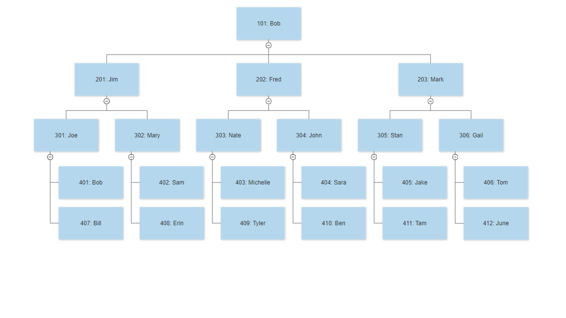
The following queries run on a table called employees, which contains the employee ID, employee name, and manager of the employee.
Let’s look at how to return the number of employees that directly or indirectly report to Bob.
Because this data is hierarchical in nature, we run a hierarchical query:
Let’s break down the preceding query and look at individual pieces that construct the components of a hierarchal query.
In general, a recursive CTE is a UNION ALL subquery with three parts within the WITH clause:
- Anchor member – The first part is a SELECT query that doesn’t have recursive reference to
cte_name. It returns the base result of the CTE, which is the initial set of the recursion. This initial query is often called the initial member, seed member, or anchor member. In the preceding query,bob_orgiscte_name, and the first SELECT query is the anchor member. - Recursive member – The second query after UNION ALL is a recursive query that references the CTE, called the recursive member. The recursive member is unioned with the anchor member (the initial seed) using the set operator UNION ALL. UNION ALL must be performed for the recursive CTEs. In the preceding example, the second query is the recursive query, and it references the CTE
bob_org. - Termination condition – This condition must be specified in the recursive member (the second query after UNION ALL). The termination condition is usually provided via a WHERE clause or JOIN operation. In the preceding example, the termination condition is provided via a WHERE clause using
e.manager = b.id.
Let’s use the same org chart to get all the subordinates of the manager with ID 302:
The first SELECT query (the anchor member) returns the base result, which is the employee with ID 302:
Next, the recursive member returns all the members underneath the tree rooted at employee ID 302 as well as the root, which is ID 302:
When we start at the seed level, recursive queries can traverse a hierarchical tree in an elegant manner. This is not easily possible without hierarchical support, which is achieved by recursive CTEs.
Display “hierarchical path” via recursive CTE
Displaying hierarchy levels and a hierarchical path along with the data is also often desired in these types of use cases. You can easily achieve this by using a recursive CTE with the following approach.
Let’s modify the preceding query to display the hierarchical path and levels:
In the preceding query, it’s very important to use CAST with the appropriate data type to define the maximum width of the result column. The main reason for using CAST is to define the column length for the resultant column. The result column data type and its length is determined by the initialization branch, namely the anchor member or first SELECT. In this example, if the employee_id column is of varchar(400) type but its actual content is much smaller, for example, 20 bytes, CAST isn’t needed when there are 10 hierarchical levels. This is because the recursive CTE’s result column path would be varchar(400), which is wide enough to hold the result data. However, if the employee_id data type is varchar(30) and the actual data length is 20 bytes, the result column path of the recursive CTE is longer than 30 bytes only after two levels of hierarchy. To accommodate 10 levels of hierarchy, CAST(employee_id as varchar(400)) is needed here. This defines the data type and size of the result column. In this case, the result column path maximum data size is 400 bytes, which is long enough to accommodate the result data. Therefore, we highly recommend using explicit CAST to define the data type and size of the result column in a recursive CTE.
The result of the preceding query is as follows:
Because both employees 402 and 408 are one level below Mary (302), their level is 1 plus Mary’s level. Also, it should be noted that the path column now indicates the hierarchical path rooted at the seed level, which was 302 in our scenario.
With these recursive CTE queries, it’s extremely easy to query hierarchical data within Amazon Redshift. No more complicated stored procedures or temporary tables are needed to query hierarchical data in Redshift.
Recursive CTE troubleshooting: Top-down vs. bottom up
You can use both top-down and bottom-up approaches via recursive CTE to traverse the hierarchical structure. In the preceding example, we presented a top-down approach. To traverse bottom-up, you should specify the starting point in the first part of the query. Then the second query needs to join the recursive component using the parent ID.
In both top-down and bottom-up strategies, you must clearly specify the termination condition. You might run into cyclic conditions, which could cause buffer overflow if termination conditions aren’t specified correctly. This could cause an infinite loop, causing Recursive CTE out of working buffers errors in Amazon Redshift. Therefore, you must add a condition to stop the recursion, which prevents infinite loops.
Summary
This post discussed the usage and benefits of the new capability in Amazon Redshift that provides support for querying hierarchical data models via recursive CTEs. This functionality can also provide tremendous benefits when combined with the SUPER data type, which provides support for querying semi-structured data like JSON. Try it out and share your experience.
About the Author
 Nadim Rana is a Data Warehouse and MPP Architect at Amazon Web Services. He is a big data enthusiast and collaborates with customers around the globe to achieve success and meet their data warehousing and data lake architecture needs.
Stable kernel updates
Announcing Fully Managed RStudio on Amazon SageMaker for Data Scientists
Post Syndicated from Channy Yun original https://aws.amazon.com/blogs/aws/announcing-fully-managed-rstudio-on-amazon-sagemaker-for-data-scientists/
Two years ago, we introduced Amazon SageMaker Studio, the industry’s first fully integrated development environment (IDE) for machine learning (ML). Amazon SageMaker Studio provides a single, web-based visual interface where you can perform all ML development steps, improving data science team productivity by up to 10 times
Many data scientists love the R project, an open-source ecosystem with more than 18,000 packages that is not just a programming language but is also an interactive environment for doing data science. RStudio is one of the most popular IDE among R developers for ML and data science projects. RStudio provides open-source tools for R and enterprise-ready professional software for data science teams to develop and share their work in the organization. But, building, securing, scaling and maintaining RStudio yourself is tedious and cumbersome.
Today, in collaboration with RStudio PBC, we are excited to announce the general availability of RStudio on Amazon SageMaker, the industry’s first fully managed RStudio Workbench IDE in the cloud. You can now bring your current RStudio license to easily migrate your self-managed RStudio environments to Amazon SageMaker in just a few simple steps. If you’d like to read more about this exciting collaboration, check out this blog from RStudio PBC.
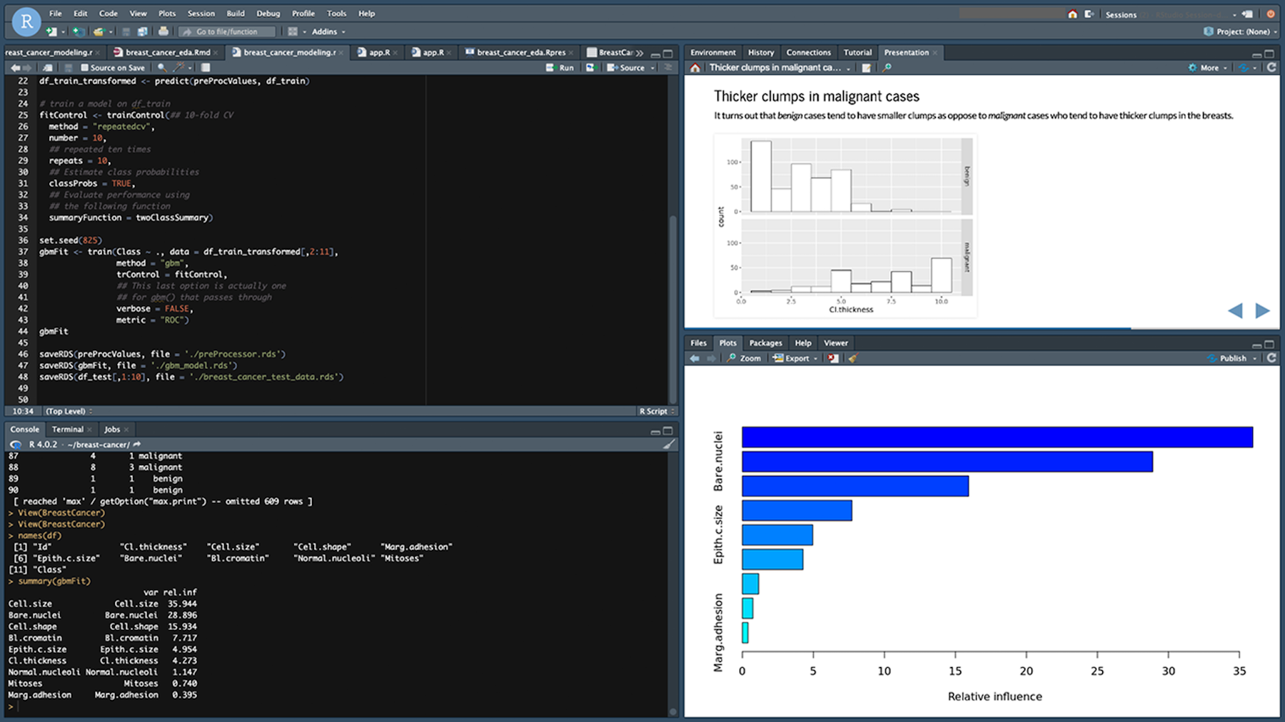
With RStudio on Amazon SageMaker, administrators can have a simple experience to migrate their RStudio environments to integrate into Amazon SageMaker and bring existing RStudio licenses to manage through AWS License Manager. They can onboard both R and Python developers to the same Amazon SageMaker domain using AWS Single Sign-On (SSO) or AWS Identity and Access Management (IAM) and take it as a centralized place to configure both RStudio and Amzon SageMaker Studio.
So, data scientists have a freedom of choice between programming languages and coding interfaces to switch between RStudio and Amazon SageMaker Studio notebooks. All of their work, including code, datasets, repositories, and other artifacts are synchronized between the two environments through the underlying Amazon EFS storage.
Getting Started with RStudio on SageMaker
You now can launch the familiar RStudio Workbench with a simple click from Amazon SageMaker. Before getting started, your administrator needs to buy an appropriate license from RStudio PBC for end-users, set up your granted licenses in AWS License Manager, and create an Amazon SageMaker domain and user profile to launch RStudio on Amazon SageMaker. To learn all the administrator jobs, including managing licenses and monitoring usages, see a blog post of the setting up process, or Manage RStudio on Amazon SageMaker in the AWS documentation.
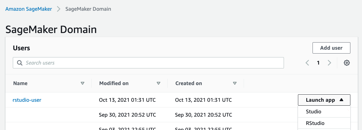
Once the required setup process is completed, you can open the RStudio Workbench from the new Launch app drop-down list in the created user list and select RStudio.
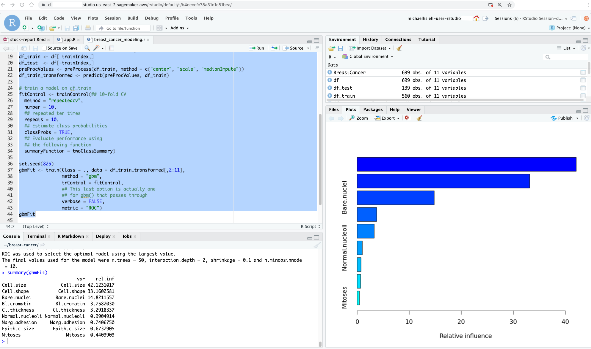
You will immediately see the RStudio Workbench home page and a list of sessions, projects, and published content on the home page. To create a new session, select the New Session button on the page, select a desired instance in the Instance Type dropdown list, and choose Start Session.

When you choose a compute instance type for a lightweight analysis that can be powered by two vCPU and four GiB memory, you can use a default ml.t3.medium instance. For a complex and large-scale ML modeling, you can choose a large instance with desired compute and memory from a wide array of ML instances available on Amazon SageMaker.
In a few minutes, your session will be ready for development in RStudio Workbench. When you launch your RStudio session, the Base R image serves as the basis of your instance. This Docker image includes R v4.0, AWS tools such as awscli, sagemaker, boto3 Python packages, and reticulate package for the interoperability between Python and R.
Managing R Packages and Publishing your Analysis
Along with the RStudio Workbench, RStudio Connect and RStudio Package Manager are the most used products of RStudio.
RStudio Connect is designed to allow data scientists to publish insights and dashboard and web applications from RStudio Workbench easily. RStudio Package Manager centrally manages the package repository for your organization so that data scientists can securely install packages faster while ensuring project reproducibility and repeatability.
Your administrator, for example, can create a repository and subscribe it to the built-in source named cran in RStudio Package Manager.
$ rspm sync --wait # Initiate a sync
$ rspm create repo --name=prod-cran --description='Access CRAN packages' # Create a repository:
$ rspm subscribe --repo=prod-cran --source=cran # Subscribe the repository to the cran source
When these steps are completed, you can use the prod-cran repository in the web interface of RStudio Package Manager.
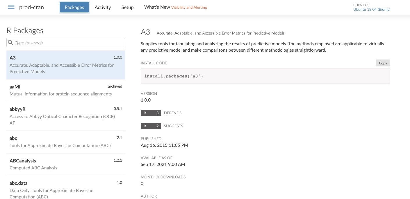
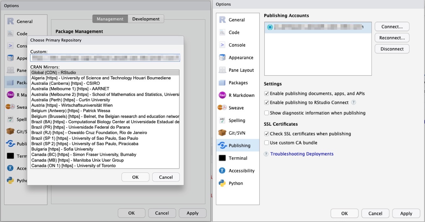
Now, you can configure this repository to install and manage your packages in RStudio Workbench. You can also configure RStudio Connect to publish insights, dashboard and web applications from RStudio Workbench via RStudio Connect so that your collaborators can easily consume your work.
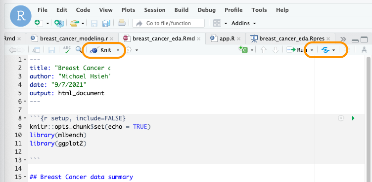
For example, you run the analysis inline to create an R Markdown that can be published to your collaborators. You can preview the slides while writing codes with the Preview button and publish it with the Publish icon in your RStudio session.
You can also publish Shiny application easy to create interactive web interfaces, or Python-based content such as Streamlit to the RStudio Connect instance.
To learn more, see Host RStudio Connect and Package Manager for ML development in RStudio on Amazon SageMaker written by my colleagues, Michael Hsieh, Chayan Panda, and Farooq Sabir on the AWS Machine Learning Blog.
Integrating training jobs with Amazon SageMaker
One of the benefits of using RStudio on Amazon SageMaker is the integration of Amazon SageMaker features. Your RStudio and Jupyter Notebook instances of Amazon SageMaker allow you to share the same Amazon EFS file system. You can import R codes written in Jupyter Notebook or use the same files in both Jupyter Notebook and RStudio without having to move your files between the two.
For example, you can run an R sample code including importing libraries, creating an Amazon SageMaker session, getting the IAM role, and importing and visualizing sample data. And then, it stores data on the S3 bucket, and triggers a training task with an XGBoost model by specifying the training container and defining an Amazon SageMaker Estimator. To learn more, see R sample codes in Amazon SageMaker.
# Import reticulate, readr and sagemaker libraries
library(reticulate)
library(readr)
sagemaker <- import('sagemaker')

# Create a sagemaker session
session <- sagemaker$Session()

# Get execution role
role_arn <- sagemaker$get_execution_role()

# Read a csv file from UCI public repository
data_file <- 'http://archive.ics.uci.edu/ml/machine-learning-databases/abalone/abalone.data'

# Copy data to a dataframe, rename columns, and show dataframe head
data_csv <- read_csv(file = data_file, col_names = FALSE, col_types = cols())
names(data_csv) <- c('sex', 'length', 'diameter', 'height', 'whole_weight', 'shucked_weight', 'viscera_weight', 'shell_weight', 'rings')
head(data_csv)

# Visualize data have height equal to 0
library(ggplot2)
options(repr.plot.width = 5, repr.plot.height = 4)
ggplot(abalone, aes(x = height, y = rings, color = sex, alpha=0.5)) + geom_point() + geom_jitter()

# Upload data to Amazon S3 bucket
s3_train <- session$upload_data(path = data_csv,
                                bucket = my_s3_bucket,
                                key_prefix = 'r_hello_world_demo/data')
s3_path = paste('s3://',bucket,'/r_hello_world_demo/data/abalone.csv',sep = '')

# Train a XGBoost model, specify the training containers, and define an Amazon SageMaker Estimator
container <- sagemaker$image_uris$retrieve(framework='xgboost',
                                           region= session$boto_region_name,
										   version='latest')
estimator <- sagemaker$estimator$Estimator(image_uri = container,
                                           role = role_arn,
                                           train_instance_count = 1L,
                                           train_instance_type = 'ml.m5.4xlarge',
                                           train_volume_size = 30L,
                                           train_max_run = 3600L,
                                           input_mode = 'File',
                                           output_path = s3_path)
Now Available
RStudio on Amazon SageMaker is available in all AWS Regions where both Amazon SageMaker Studio and AWS License Manager are available. You can bring your own license of RStudio on Amazon SageMaker and pay for the underlying compute and storage resources within Amazon SageMaker or other AWS services, based on your usage.
To get started with RStudio on Amazon SageMaker, you can use AWS Free Tier. You can use 250 hours of ml.t3.medium instance on Amazon SageMaker Studio per month for the first two months. To learn more, see Amazon SageMaker Pricing page.
Give it a try, and please send us feedback either in the AWS forum for Amazon SageMaker or through your usual AWS support contacts.
– Channy
Implement OAuth 2.0 device grant flow by using Amazon Cognito and AWS Lambda
Post Syndicated from Jeff Lombardo original https://aws.amazon.com/blogs/security/implement-oauth-2-0-device-grant-flow-by-using-amazon-cognito-and-aws-lambda/
In this blog post, you’ll learn how to implement the OAuth 2.0 device authorization grant flow for Amazon Cognito by using AWS Lambda and Amazon DynamoDB.
When you implement the OAuth 2.0 authorization framework (RFC 6749) for internet-connected devices with limited input capabilities or that lack a user-friendly browser—such as wearables, smart assistants, video-streaming devices, smart-home automation, and health or medical devices—you should consider using the OAuth 2.0 device authorization grant (RFC 8628). This authorization flow makes it possible for the device user to review the authorization request on a secondary device, such as a smartphone, that has more advanced input and browser capabilities. By using this flow, you can work around the limits of the authorization code grant flow with Proof Key for Code Exchange (PKCE)-defined OpenID Connect Core specifications. This will help you to avoid scenarios such as:
- Forcing end users to define a dedicated application password or use an on-screen keyboard with a remote control
- Degrading the security posture of the end users by exposing their credentials to the client application or external observers
One common example of this type of scenario is a TV HDMI streaming device where, to be able to consume videos, the user must slowly select each letter of their user name and password with the remote control, which exposes these values to other people in the room during the operation.
Solution overview
The OAuth 2.0 device authorization grant (RFC 8628) is an IETF standard that enables Internet of Things (IoT) devices to initiate a unique transaction that authenticated end users can securely confirm through their native browsers. After the user authorizes the transaction, the solution will issue a delegated OAuth 2.0 access token that represents the end user to the requesting device through a back-channel call, as shown in Figure 1.
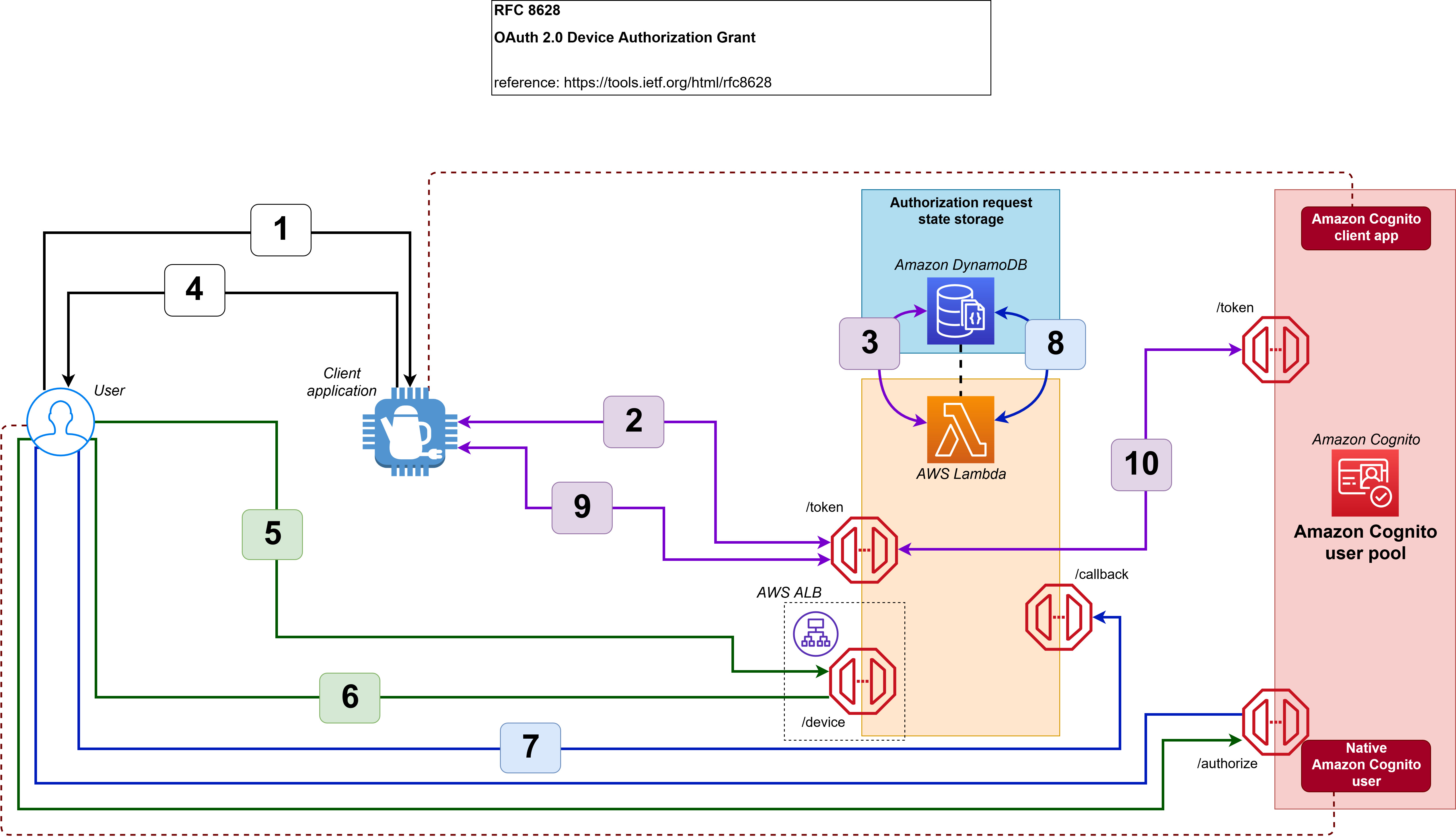
Figure 1: The device grant flow implemented in this solution
The workflow is as follows:
- An unauthenticated user requests service from the device.
- The device requests a pair of random codes (one for the device and one for the user) by authenticating with the client ID and client secret.
- The Lambda function creates an authorization request that stores the device code, user code, scope, and requestor’s client ID.
- The device provides the user code to the user.
- The user enters their user code on an authenticated web page to authorize the client application.
- The user is redirected to the Amazon Cognito user pool /authorize endpoint to request an authorization code.
- The user is returned to the Lambda function /callback endpoint with an authorization code.
- The Lambda function stores the authorization code in the authorization request.
- The device uses the device code to check the status of the authorization request regularly. And, after the authorization request is approved, the device uses the device code to retrieve a set of JSON web tokens from the Lambda function.
- In this case, the Lambda function impersonates the device to the Amazon Cognito user pool /token endpoint by using the authorization code that is stored in the authorization request, and returns the JSON web tokens to the device.
To achieve this flow, this blog post provides a solution that is composed of:
- An AWS Lambda function with three additional endpoints:
- The /token endpoint, which will handle client application requests such as generation of codes, the authorization request status check, and retrieval of the JSON web tokens.
- The /device endpoint, which will handle user requests such as delivering the UI for approval or denial of the authorization request, or retrieving an authorization code.
- The /callback endpoint, which will handle the reception of the authorization code associated with the user who is approving or denying the authorization request.
- An Amazon Cognito user pool with:
- Two Amazon Cognito app clients, each with a client ID and client secret. One app client is for the client application, and one is for the Elastic Load Balancing Application Load Balancer that protects the /device endpoint.
- One Amazon Cognito user for testing purposes.
- Finally, an Amazon DynamoDB table to store the state of all the processed authorization requests.
Implement the solution
The implementation of this solution requires three steps:
- Define the public fully qualified domain name (FQDN) for the Application Load Balancer public endpoint and associate an X.509 certificate to the FQDN
- Deploy the provided AWS CloudFormation template
- Configure the DNS to point to the Application Load Balancer public endpoint for the public FQDN
Step 1: Choose a DNS name and create an SSL certificate
Your Lambda function endpoints must be publicly resolvable when they are exposed by the Application Load Balancer through an HTTPS/443 listener.
To configure the Application Load Balancer component
- Choose an FQDN in a DNS zone that you own.
- Associate an X.509 certificate and private key to the FQDN by doing one of the following:
- Generate the certificate and private key directly within AWS Certificate Manager (ACM)
- OR import the certificate and private key into ACM
- After you have the certificate in ACM, navigate to the Certificates page in the ACM console.
- Choose the right arrow (►) icon next to your certificate to show the certificate details.

Figure 2: Locating the certificate in ACM
- Copy the Amazon Resource Name (ARN) of the certificate and save it in a text file.

Figure 3: Locating the certificate ARN in ACM


Step 2: Deploy the solution by using a CloudFormation template
To configure this solution, you’ll need to deploy the solution CloudFormation template.
Before you deploy the CloudFormation template, you can view it in its GitHub repository.
To deploy the CloudFormation template
- Choose the following Launch Stack button to launch a CloudFormation stack in your account.

Note: The stack will launch in the N. Virginia (us-east-1) Region. To deploy this solution into other AWS Regions, download the solution’s CloudFormation template, modify it, and deploy it to the selected Region.
- During the stack configuration, provide the following information:
- A name for the stack.
- The ARN of the certificate that you created or imported in AWS Certificate Manager.
- A valid email address that you own. The initial password for the Amazon Cognito test user will be sent to this address.
- The FQDN that you chose earlier, and that is associated to the certificate that you created or imported in AWS Certificate Manager.

Figure 4: Configure the CloudFormation stack
- After the stack is configured, choose Next, and then choose Next again. On the Review page, select the check box that authorizes CloudFormation to create AWS Identity and Access Management (IAM) resources for the stack.

Figure 5: Authorize CloudFormation to create IAM resources
- Choose Create stack to deploy the stack. The deployment will take several minutes. When the status says CREATE_COMPLETE, the deployment is complete.



Step 3: Finalize the configuration
After the stack is set up, you must finalize the configuration by creating a DNS CNAME entry in the DNS zone you own that points to the Application Load Balancer DNS name.
To create the DNS CNAME entry
- In the CloudFormation console, on the Stacks page, locate your stack and choose it.

Figure 6: Locating the stack in CloudFormation
- Choose the Outputs tab.
- Copy the value for the key ALBCNAMEForDNSConfiguration.

Figure 7: The ALB CNAME output in CloudFormation
- Configure a CNAME DNS entry into your DNS hosted zone based on this value. For more information on how to create a CNAME entry to the Application Load Balancer in a DNS zone, see Creating records by using the Amazon Route 53 console.
- Note the other values in the Output tab, which you will use in the next section of this post.
Output key Output value and function DeviceCognitoClientClientID The app client ID, to be used by the simulated device to interact with the authorization server DeviceCognitoClientClientSecret The app client secret, to be used by the simulated device to interact with the authorization server TestEndPointForDevice The HTTPS endpoint that the simulated device will use to make its requests TestEndPointForUser The HTTPS endpoint that the user will use to make their requests UserPassword The password for the Amazon Cognito test user UserUserName The user name for the Amazon Cognito test user


Evaluate the solution
Now that you’ve deployed and configured the solution, you can initiate the OAuth 2.0 device code grant flow.
Until you implement your own device logic, you can perform all of the device calls by using the curl library, a Postman client, or any HTTP request library or SDK that is available in the client application coding language.
All of the following device HTTPS requests are made with the assumption that the device is a private OAuth 2.0 client. Therefore, an HTTP Authorization Basic header will be present and formed with a base64-encoded Client ID:Client Secret value.
You can retrieve the URI of the endpoints, the client ID, and the client secret from the CloudFormation Output table for the deployed stack, as described in the previous section.
Initialize the flow from the client application
The solution in this blog post lets you decide how the user will ask the device to start the authorization request and how the user will be presented with the user code and URI in order to verify the request. However, you can emulate the device behavior by generating the following HTTPS POST request to the Application Load Balancer–protected Lambda function /token endpoint with the appropriate HTTP Authorization header. The Authorization header is composed of:
- The prefix Basic, describing the type of Authorization header
- A space character as separator
- The base64 encoding of the concatenation of:
- The client ID
- The colon character as a separator
- The client secret
The following JSON message will be returned to the client application.
Check the status of the authorization request from the client application
You can emulate the process where the client app regularly checks for the authorization request status by using the following HTTPS POST request to the Application Load Balancer–protected Lambda function /token endpoint. The request should have the same HTTP Authorization header that was defined in the previous section.
Until the authorization request is approved, the client application will receive an error message that includes the reason for the error: authorization_pending if the request is not yet authorized, slow_down if the polling is too frequent, or expired if the maximum lifetime of the code has been reached. The following example shows the authorization_pending error message.
Approve the authorization request with the user code
Next, you can approve the authorization request with the user code. To act as the user, you need to open a browser and navigate to the verification_uri that was provided by the client application.
If you don’t have a session with the Amazon Cognito user pool, you will be required to sign in.
Note: Remember that the initial password was sent to the email address you provided when you deployed the CloudFormation stack.
If you used the initial password, you’ll be asked to change it. Make sure to respect the password policy when you set a new password. After you’re authenticated, you’ll be presented with an authorization page, as shown in Figure 8.
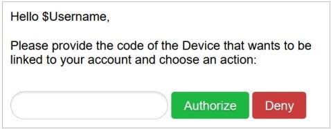
Figure 8: The user UI for approving or denying the authorization request
Fill in the user code that was provided by the client application, as in the previous step, and then choose Authorize.
When the operation is successful, you’ll see a message similar to the one in Figure 9.

Figure 9: The “Success” message when the authorization request has been approved
Finalize the flow from the client app
After the request has been approved, you can emulate the final client app check for the authorization request status by using the following HTTPS POST request to the Application Load Balancer–protected Lambda function /token endpoint. The request should have the same HTTP Authorization header that was defined in the previous section.
The JSON web token set will then be returned to the client application, as follows.
The client application can now consume resources on behalf of the user, thanks to the access token, and can refresh the access token autonomously, thanks to the refresh token.
Going further with this solution
This project is delivered with a default configuration that can be extended to support additional security capabilities or to and adapted the experience to your end-users’ context.
Extending security capabilities
Through this solution, you can:
- Use an AWS KMS key issued by AWS KMS to:
- Encrypt the data in the database;
- Protect the configuration in the Amazon Lambda function;
- Use AWS Secret Manager to:
- Securely store sensitive information like Cognito application client’s credentials;
- Enforce Cognito application client’s credentials rotation;
- Implement additional Amazon Lambda’s code to enforce data integrity on changes;
- Activate AWS WAF WebACLs to protect your endpoints against attacks;
Customizing the end-user experience
The following table shows some of the variables you can work with.
| Name | Function | Default value | Type |
| CODE_EXPIRATION | Represents the lifetime of the codes generated | 1800 | Seconds |
| DEVICE_CODE_FORMAT | Represents the format for the device code | #aA | A string where: # represents numbers a lowercase letters A uppercase letters ! special characters |
| DEVICE_CODE_LENGTH | Represents the device code length | 64 | Number |
| POLLING_INTERVAL | Represents the minimum time, in seconds, between two polling events from the client application | 5 | Seconds |
| USER_CODE_FORMAT | Represents the format for the user code | #B | A string where: # represents numbers a lowercase letters b lowercase letters that aren’t vowels A uppercase letters B uppercase letters that aren’t vowels ! special characters |
| USER_CODE_LENGTH | Represents the user code length | 8 | Number |
| RESULT_TOKEN_SET | Represents what should be returned in the token set to the client application | ACCESS+REFRESH | A string that includes only ID, ACCESS, and REFRESH values separated with a + symbol |
To change the values of the Lambda function variables
- In the Lambda console, navigate to the Functions page.
- Select the DeviceGrant-token function.

Figure 10: AWS Lambda console—Function selection
- Choose the Configuration tab.

Figure 11: AWS Lambda function—Configuration tab
- Select the Environment variables tab, and then choose Edit to change the values for the variables.

Figure 12: AWS Lambda Function—Environment variables tab
- Generate new codes as the device and see how the experience changes based on how you’ve set the environment variables.


Conclusion
Although your business and security requirements can be more complex than the example shown in this post, this blog post will give you a good way to bootstrap your own implementation of the Device Grant Flow (RFC 8628) by using Amazon Cognito, AWS Lambda, and Amazon DynamoDB.
Your end users can now benefit from the same level of security and the same experience as they have when they enroll their identity in their mobile applications, including the following features:
- Credentials will be provided through a full-featured application on the user’s mobile device or their computer
- Credentials will be checked against the source of authority only
- The authentication experience will match the typical authentication process chosen by the end user
- Upon consent by the end user, IoT devices will be provided with end-user delegated dynamic credentials that are bound to the exact scope of tasks for that device
If you have feedback about this post, submit comments in the Comments section below. If you have questions about this post, start a new thread on the Amazon Cognito forum or reach out through the post’s GitHub repository.
Want more AWS Security how-to content, news, and feature announcements? Follow us on Twitter.
Firefox 94.0 and Firefox ESR 91.3.0
Post Syndicated from original https://lwn.net/Articles/874832/rss
Firefox 94.0 has been
released. Linux users should see improved
WebGL performance and reduced power consumption for many workloads. The
about:unloads
page shows the user information about open tabs and allows them to release
system resources by unloading tabs without closing them. Site
Isolation provides better protection against side-channel attacks. See
the announcement for more new features in this release.
Firefox ESR
91.3 is also available, with various stability, functionality, and security
fixes.
Backblaze Announces Launch of Initial Public Offering
Post Syndicated from Backblaze original https://www.backblaze.com/blog/backblaze-announces-launch-of-initial-public-offering/
SAN MATEO—November 2, 2021. Backblaze, Inc. (“Backblaze”), a leading storage cloud platform, today announced that it has launched the roadshow for its initial public offering. Backblaze has filed a registration statement on Form S-1 with the Securities and Exchange Commission (the “SEC”) to offer 6,250,000 shares of its Class A common stock to the public. In addition, the underwriters will have a 30-day option to purchase up to an additional 937,500 shares of Class A common stock from Backblaze. The initial public offering price is expected to be between $15.00 and $17.00 per share. Backblaze has applied to list its Class A common stock on the Nasdaq Global Market under the ticker symbol “BLZE.”
Oppenheimer & Co., William Blair and Raymond James will act as lead book-running managers for the proposed offering, with JMP Securities and B. Riley Securities acting as joint book-running managers. Lake Street will act as co-manager for the proposed offering.
The offering will be made only by means of a prospectus. Copies of the preliminary prospectus related to the offering may be obtained, when available, from Oppenheimer & Co. Inc., Attention: Syndicate Prospectus Department, 85 Broad St., 26th Floor, New York, NY 10004, by telephone at (212) 667-8055, or by email at [email protected]; William Blair & Company, L.L.C. Attention: Prospectus Department, 150 North Riverside Plaza, Chicago, IL 60606, or by telephone at (800) 621-0687 or by email at [email protected]; or Raymond James & Associates, Inc., 880 Carillon Parkway, St. Petersburg, FL 33716, email: [email protected], telephone: 800-248-8863.
A registration statement relating to the proposed sale of these securities has been filed with the SEC but has not yet become effective. These securities may not be sold, nor may offers to buy be accepted, prior to the time the registration statement becomes effective. This press release shall not constitute an offer to sell or the solicitation of an offer to buy, nor shall there be any sale of these securities in any state or jurisdiction in which such offer, solicitation, or sale would be unlawful prior to registration or qualification under the securities laws of any such state or jurisdiction.
The post Backblaze Announces Launch of Initial Public Offering appeared first on Backblaze Blog | Cloud Storage & Cloud Backup.
Netflix Video Quality at Scale with Cosmos Microservices
Post Syndicated from Netflix Technology Blog original https://netflixtechblog.com/netflix-video-quality-at-scale-with-cosmos-microservices-552be631c113
by Christos G. Bampis, Chao Chen, Anush K. Moorthy and Zhi Li
Introduction
Measuring video quality at scale is an essential component of the Netflix streaming pipeline. Perceptual quality measurements are used to drive video encoding optimizations, perform video codec comparisons, carry out A/B testing and optimize streaming QoE decisions to mention a few. In particular, the VMAF metric lies at the core of improving the Netflix member’s streaming video quality. It has become a de facto standard for perceptual quality measurements within Netflix and, thanks to its open-source nature, throughout the video industry.
As VMAF evolves and is integrated with more encoding and streaming workflows within Netflix, we need scalable ways of fostering video quality innovations. For example, when we design a new version of VMAF, we need to effectively roll it out throughout the entire Netflix catalog of movies and TV shows. This article explains how we designed microservices and workflows on top of the Cosmos platform to bolster such video quality innovations.
The coupling problem
Until recently, video quality measurements were generated as part of our Reloaded production system. This system is responsible for processing incoming media files, such as video, audio and subtitles, and making them playable on the streaming service. The Reloaded system is a well-matured and scalable system, but its monolithic architecture can slow down rapid innovation. More importantly, within Reloaded, video quality measurements are generated together with video encoding. This tight coupling means that it is not possible to achieve the following without re-encoding:
A) rollout of new video quality algorithms
B) maintaining the data quality of our catalog (e.g. via bug fixes).
Re-encoding the entire catalog in order to generate updated quality scores is an extremely costly solution and hence infeasible. Such coupling problems abound with our Reloaded architecture, and hence the Media Cloud Engineering and Encoding Technologies teams have been working together to develop a solution that addresses many of the concerns with our previous architecture. We call this system Cosmos.
Cosmos is a computing platform for workflow-driven, media-centric microservices. Cosmos offers several benefits as highlighted in the linked blog, such as separation of concerns, independent deployments, observability, rapid prototyping and productization. Here, we describe how we architected the video quality service using Cosmos and how we managed the migration from Reloaded to Cosmos for video quality computations while running a production system.
Video quality as a service
In Cosmos, all video quality computations are performed by an independent microservice called the Video Quality Service (VQS). VQS takes as input two videos: a source and its derivative, and returns back the measured perceptual quality of the derivative. The measured quality could be a single value, in cases where only a single metric’s output is needed (e.g., VMAF), or it could also return back multiple perceptual quality scores, in cases where the request asks for such computation (e.g., VMAF and SSIM).
VQS, like most Cosmos services, consists of three domain-specific and scale-agnostic layers. Each layer is built on top of a corresponding scale-aware Cosmos subsystem. There is an external-facing API layer (Optimus), a rule-based video quality workflow layer (Plato) and a serverless compute layer (Stratum). The inter-layer communication is based on our internally developed and maintained Timestone queuing system. The figure below shows each layer and the corresponding Cosmos subsystem in parenthesis.
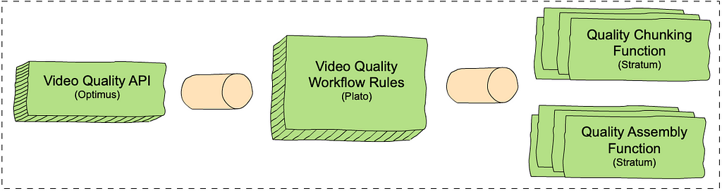
- The VQS API layer exposes endpoints: one to request quality measurements (measureQuality) and one to get quality results asynchronously (getQuality).
- The VQS workflow layer consists of rules that determine how to measure video quality. Similar to chunk-based encoding, the VQS workflow consists of chunk-based quality calculations, followed by an assembly step. This enables us to use our scale to increase throughput and reduce latencies. The chunk-based quality step computes the quality for each chunk and the assembly step combines the results of all quality computations. For example, if we have two chunks with two and three frames and VMAF scores of [50, 60] and [80, 70, 90] respectively, the assembly step combines the scores into [50, 60, 80, 70, 90]. The chunking rule calls out to the chunk-based quality computation function in Stratum (see below) for all the chunks in the video, and the assembly rule calls out to the assembly function.
- The VQS Stratum layer consists of two functions, which perform the chunk-based quality calculation and assembly.
Deep dive into the VQS workflow
The following trace graph from our observability portal, Nirvana, sheds more light on how VQS works. The request provides the source and the derivative whose quality is to be computed and requests that the VQS provides quality scores using VMAF, PSNR and SSIM as quality metrics.

Here is a step-by-step description of the processes involved:
1. VQS is called using the measureQuality endpoint. The VQS API layer will translate the external request into VQS-specific data models.
2. The workflow is initiated. Here, based on the video length, the throughput and latency requirements, available scale etc., the VQS workflow decides that it will split the quality computation across two chunks and hence, it creates two messages (one for each chunk) to be executed independently by the chunk-based quality computation Stratum function. All three requested quality metrics will be calculated for each chunk.
3. Quality calculation begins for each chunk. The figure does not show the chunk start times separately, however, each chunked quality computation starts and completes (annotated as 3a and 3b) independently based on resource availability.
3b. Plato initiates assembly once all chunked quality computations complete.
4. Assembly begins, with separate invocations to the assembler stratum functions for each metric. As before, the start time for each metric’s assembly can vary. Such separation of computation allows us to fail partially, return early, scale independently depending on metric complexity etc.
4a & 4b. Assembly for two of the metrics (e.g. PSNR and SSIM) is complete.
4c & 5. Assembly for VMAF is complete and the entire workflow is thus completed. The quality results are now available to the caller via the getQuality endpoint.
The above is a simplified illustration of the workflow, however, in practice, the actual design is extremely flexible, and supports a variety of features, including different quality metrics, adaptive chunking strategies, producing quality at different temporal granularities (frame-level, segment level and aggregate) and measuring quality for different use cases, such as measuring quality for different device types (like a phone), SDR, HDR and others.
Living a double life
While VQS is a dedicated video quality microservice that addresses the aforementioned coupling with video encoding, there is another aspect to be addressed. The entire Reloaded system is currently being migrated into Cosmos. This is a big, cross-team effort which means that some applications are still in Reloaded, while others have already made it into Cosmos. How do we leverage VQS, while some applications that consume video quality measurements are still in Reloaded? In other words, how do we manage living a life in both worlds?
A bridge between two worlds
To live such a life, we developed several “bridging” workflows, which allow us to route video quality traffic from Reloaded into Cosmos. Each of these workflows also acts as a translator of Reloaded data models into appropriate Cosmos-service data models. Meanwhile, Cosmos-only workflows can be integrated with VQS without the need for bridging. This allows us to not only operate in both worlds and provide existing video quality features, but also roll out new features ubiquitously (either for Reloaded or Cosmos customer applications).

Data conversions as a service
To complete our design, we have to solve one last puzzle. While we have a way to call VQS, the VQS output is designed to avoid the centralized data modeling of Reloaded. For example, VQS relies on the Netflix Media Database (NMDB) to store and index the quality scores, while the Reloaded system uses a mix of non-queryable data models and files. To aid our transition, we introduced another Cosmos microservice: the Document Conversion Service (DCS). DCS is responsible for converting between Cosmos data models and Reloaded data models. Further, DCS also interfaces with NMDB and hence is capable of converting from the data store to Reloaded file-based data and vice-versa. DCS has several other end points that perform similar data conversion when needed so the above described Roman-riding can occur gracefully.

Where we are now and what’s next
We have migrated almost all of our video quality computations from Reloaded into Cosmos. VQS currently represents the largest workload fueled by the Cosmos platform. Video quality has matured in Cosmos and we are invested in making VQS more flexible and efficient. Besides supporting existing video quality features, all our new video quality features have been developed in VQS. Stay tuned for more details on these algorithmic innovations.
Acknowledgments
This work was made possible with the help of many stunning Netflix colleagues. We would like to thank George Ye and Sujana Sooreddy for their contributions to the Reloaded-Cosmos bridge development, Ameya Vasani and Frank San Miguel for contributing to power up VQS at scale and Susie Xia for helping with performance analysis. Also, the Media Content Playback team, the Media Compute/Storage Infrastructure team and the entire Cosmos platform team that brought Cosmos to life and whole-heartedly supported us in our venture into Cosmos.
If you are interested in becoming a member of our team, we are hiring! Our current job postings can be found here:
https://jobs.netflix.com/jobs/101109705
https://jobs.netflix.com/jobs/127695186
https://jobs.netflix.com/jobs/126802582

Netflix Video Quality at Scale with Cosmos Microservices was originally published in Netflix TechBlog on Medium, where people are continuing the conversation by highlighting and responding to this story.
Generating DevOps Guru Proactive Insights for Amazon ECS
Post Syndicated from Trishanka Saikia original https://aws.amazon.com/blogs/devops/generate-devops-guru-proactive-insights-in-ecs-using-container-insights/
Monitoring is fundamental to operating an application in production, since we can only operate what we can measure and alert on. As an application evolves, or the environment grows more complex, it becomes increasingly challenging to maintain monitoring thresholds for each component, and to validate that they’re still set to an effective value. We not only want monitoring alarms to trigger when needed, but also want to minimize false positives.
Amazon DevOps Guru is an AWS service that helps you effectively monitor your application by ingesting vended metrics from Amazon CloudWatch. It learns your application’s behavior over time and then detects anomalies. Based on these anomalies, it generates insights by first combining the detected anomalies with suspected related events from AWS CloudTrail, and then providing the information to you in a simple, ready-to-use dashboard when you start investigating potential issues. Amazon DevOpsGuru makes use of the CloudWatch Containers Insights to detect issues around resource exhaustion for Amazon ECS or Amazon EKS applications. This helps in proactively detecting issues like memory leaks in your applications before they impact your users, and also provides guidance as to what the probable root-causes and resolutions might be.
This post will demonstrate how to simulate a memory leak in a container running in Amazon ECS, and have it generate a proactive insight in Amazon DevOps Guru.
Solution Overview
The following diagram shows the environment we’ll use for our scenario. The container “brickwall-maker” is preconfigured as to how quickly to allocate memory, and we have built this container image and published it to our public Amazon ECR repository. Optionally, you can build and host the docker image in your own private repository as described in step 2 & 3.
After creating the container image, we’ll utilize an AWS CloudFormation template to create an ECS Cluster and an ECS Service called “Test” with a desired count of two. This will create two tasks using our “brickwall-maker” container image. The stack will also enable Container Insights for the ECS Cluster. Then, we will enable resource coverage for this CloudFormation stack in Amazon DevOpsGuru in order to start our resource analysis.

Source provided on GitHub:
- DevOpsGuru.yaml
- EnableDevOpsGuruForCfnStack.yaml
- Docker container source
Steps:
1. Create your IDE environment
In the AWS Cloud9 console, click Create environment, give your environment a Name, and click Next step. On the Environment settings page, change the instance type to t3.small, and click Next step. On the Review page, make sure that the Name and Instance type are set as intended, and click Create environment. The environment creation will take a few minutes. After that, the AWS Cloud9 IDE will open, and you can continue working in the terminal tab displayed in the bottom pane of the IDE.
Install the following prerequisite packages, and ensure that you have docker installed:
sudo yum install -y docker
sudo service docker start
docker --version2. Optional : Create ECR private repository
If you want to build your own container image and host it in your own private ECR repository, create a new repository with the following command and then follow the steps to prepare your own image:
3. Optional: Prepare Docker Image
Authenticate to Amazon Elastic Container Registry (ECR) in the target region
In the above command, as well as in the following shown below, make sure that you replace 123456789012 with your own account ID.
Build brickwall-maker Docker container:
Tag the Docker container to prepare it to be pushed to ECR:
Push the built Docker container to ECR
4. Launch the CloudFormation template to deploy your ECS infrastructure
To deploy your ECS infrastructure, run the following command (replace your own private ECR URL or use our public URL) in the ParameterValue) to launch the CloudFormation template :
5. Enable DevOps Guru to monitor the ECS Application
Run the following command to enable DevOps Guru for monitoring your ECS application:
6. Wait for base-lining of resources
This step lets DevOps Guru complete the baselining of the resources and benchmark the normal behavior. For this particular scenario, we recommend waiting two days before any insights are triggered.
Unlike other monitoring tools, the DevOps Guru dashboard would not present any counters or graphs. In the meantime, you can utilize CloudWatch Container Insights to monitor the cluster-level, task-level, and service-level metrics in ECS.
7. View Container Insights metrics
- Open the CloudWatch console.
- In the navigation pane, choose Container Insights.
- Use the drop-down boxes near the top to select ECS Services as the resource type to view, then select DevOps Guru as the resource to monitor.
- The performance monitoring view will show you graphs for several metrics, including “Memory Utilization”, which you can watch increasing from here. In addition, it will show the list of tasks in the lower “Task performance” pane showing the “Avg CPU” and “Avg memory” metrics for the individual tasks.
8. Review DevOps Guru insights
When DevOps Guru detects an anomaly, it generates a proactive insight with the relevant information needed to investigate the anomaly, and it will list it in the DevOps Guru Dashboard.
You can view the insights by clicking on the number of insights displayed in the dashboard. In our case, we expect insights to be shown in the “proactive insights” category on the dashboard.
Once you have opened the insight, you will see that the insight view is divided into the following sections:
- Insight Overview with a basic description of the anomaly. In this case, stating that Memory Utilization is approaching limit with details of the stack that is being affected by the anomaly.
- Anomalous metrics consisting of related graphs and a timeline of the predicted impact time in the future.
- Relevant events with contextual information, such as changes or updates made to the CloudFormation stack’s resources in the region.
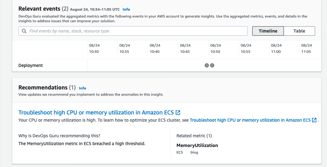
- Recommendations to mitigate the issue. As seen in the following screenshot, it recommends troubleshooting High CPU or Memory Utilization in ECS along with a link to the necessary documentation.
The following screenshot illustrates an example insight detail page from DevOps Guru

Conclusion
This post describes how DevOps Guru continuously monitors resources in a particular region in your AWS account, as well as proactively helps identify problems around resource exhaustion such as running out of memory, in advance. This helps IT operators take preventative actions even before a problem presents itself, thereby preventing downtime.
Cleaning up
After walking through this post, you should clean up and un-provision the resources in order to avoid incurring any further charges.
- To un-provision the CloudFormation stacks, on the AWS CloudFormation console, choose Stacks. Select the stack name, and choose Delete.
- Delete the AWS Cloud9 environment.
- Delete the ECR repository.
About the authors
Exploring Data Transfer Costs for AWS Managed Databases
Post Syndicated from Dennis Schmidt original https://aws.amazon.com/blogs/architecture/exploring-data-transfer-costs-for-aws-managed-databases/
When selecting managed database services in AWS, it’s important to understand how data transfer charges are calculated – whether it’s relational, key-value, document, in-memory, graph, time series, wide column, or ledger.
This blog will outline the data transfer charges for several AWS managed database offerings to help you choose the most cost-effective setup for your workload.
This blog illustrates pricing at the time of publication and assumes no volume discounts or applicable taxes and duties. For demonstration purposes, we list the primary AWS Region as US East (Northern Virginia) and the secondary Region is US West (Oregon). Always refer to the individual service pricing pages for the most up-to-date pricing.
Data transfer between AWS and internet
There is no charge for inbound data transfer across all services in all Regions. When you transfer data from AWS resources to the internet, you’re charged per service, with rates specific to the originating Region. Figure 1 illustrates data transfer charges that accrue from AWS services discussed in this blog out to the public internet in the US East (Northern Virginia) Region.

Figure 1. Data transfer to the internet
The remainder of this blog will focus on data transfer within AWS.
Data transfer with Amazon RDS
Amazon Relational Database Service (Amazon RDS) makes it straightforward to set up, operate, and scale a relational database in the cloud. Amazon RDS provides six database engines to choose from: Amazon Aurora, MySQL, MariaDB, Oracle, SQL Server, and PostgreSQL.
Let’s consider an application running on Amazon Elastic Compute Cloud (Amazon EC2) that uses Amazon RDS as a data store.
Figure 2 illustrates where data transfer charges apply. For clarity, we have left out connection points to the replica servers – this is addressed in Figure 3.

Figure 2. Amazon RDS data transfer
In this setup, you will not incur charges for:
- Data transfer to or from Amazon EC2 in the same Region, Availability Zone, and virtual private cloud (VPC)
You will accrue charges for data transfer between:
- Amazon EC2 and Amazon RDS across Availability Zones within the same VPC, charged at Amazon EC2 and Amazon RDS ($0.01/GB in and $0.01/GB out)
- Amazon EC2 and Amazon RDS across Availability Zones and across VPCs, charged at Amazon EC2 only ($0.01/GB in and $0.01/GB out). For Aurora, this is charged at Amazon EC2 and Aurora ($0.01/GB in and $0.01/GB out)
- Amazon EC2 and Amazon RDS across Regions, charged on both sides of the transfer ($0.02/GB out)
Figure 3 illustrates several features that are available within Amazon RDS to show where data transfer charges apply. These include multi-Availability Zone deployment, read replicas, and cross-Region automated backups. Not all database engines support all features, consult the product documentation to learn more.

Figure 3. Amazon RDS features
In this setup, you will not incur data transfer charges for:
- Data replication in a multi-Availability Zone deployment or to read replicas within the same Region
- Transfer of snapshots to Amazon Simple Storage Service (Amazon S3) in the same Region
In addition to the charges you will incur when you transfer data to the internet, you will accrue data transfer charges for:
- Data replication to read replicas deployed across Regions ($0.02/GB out)
- Regional transfers for Amazon RDS snapshot copies or automated cross-Region backups ($0.02/GB out)
Refer to the following pricing pages for more detail:
- Amazon Aurora
- Amazon RDS for MySQL
- Amazon RDS for MariaDB
- Amazon RDS for Oracle
- Amazon RDS for SQL Server
- Amazon RDS for PostgreSQL
Data transfer with Amazon DynamoDB
Amazon DynamoDB is a key-value and document database that delivers single-digit millisecond performance at any scale. Figures 4 and 5 illustrate an application hosted on Amazon EC2 that uses DynamoDB as a data store and includes DynamoDB global tables and DynamoDB Accelerator (DAX).

Figure 4. DynamoDB with global tables

Figure 5. DynamoDB without global tables
You will not incur data transfer charges for:
- Inbound data transfer to DynamoDB
- Data transfer between DynamoDB and Amazon EC2 in the same Region
- Data transfer between Amazon EC2 and DAX in the same Availability Zone
In addition to the charges you will incur when you transfer data to the internet, you will accrue charges for data transfer between:
- Amazon EC2 and DAX across Availability Zones, charged at the EC2 instance ($0.01/GB in and $0.01/GB out)
- Global tables for cross-Region replication or adding replicas to tables that contain data in DynamoDB, charged at the source Region, as shown in Figure 4 ($0.02/GB out)
- Amazon EC2 and DynamoDB across Regions, charged on both sides of the transfer, as shown in Figure 5 ($0.02/GB out)
Refer to the DynamoDB pricing page for more detail.
Data transfer with Amazon Redshift
Amazon Redshift is a cloud data warehouse that makes it fast and cost-effective to analyze your data using standard SQL and your existing business intelligence tools. There are many integrations and services available to query and visualize data within Amazon Redshift. To illustrate data transfer costs, Figure 6 shows an EC2 instance running a consumer application connecting to Amazon Redshift over JDBC/ODBC.

Figure 6. Amazon Redshift data transfer
You will not incur data transfer charges for:
- Data transfer within the same Availability Zone
- Data transfer to Amazon S3 for backup, restore, load, and unload operations in the same Region
In addition to the charges you will incur when you transfer data to the internet, you will accrue charges for the following:
- Across Availability Zones, charged on both sides of the transfer ($0.01/GB in and $0.01/GB out)
- Across Regions, charged on both sides of the transfer ($0.02/GB out)
Refer to the Amazon Redshift pricing page for more detail.
Data transfer with Amazon DocumentDB
Amazon DocumentDB (with MongoDB compatibility) is a database service that is purpose-built for JSON data management at scale. Figure 7 illustrates an application hosted on Amazon EC2 that uses Amazon DocumentDB as a data store, with read replicas in multiple Availability Zones and cross-Region replication for Amazon DocumentDB Global Clusters.
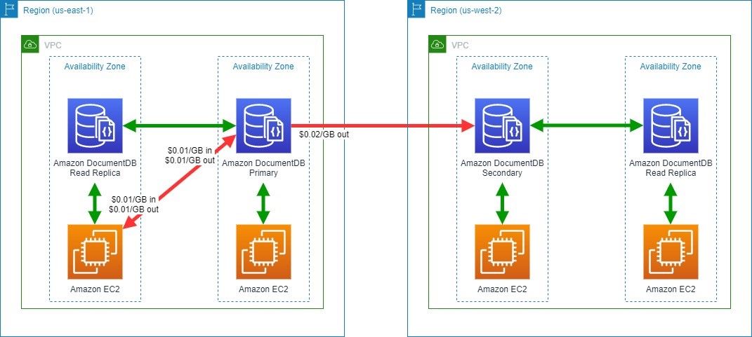
Figure 7. Amazon DocumentDB data transfer
You will not incur data transfer charges for:
- Data transfer between Amazon DocumentDB and EC2 instances in the same Availability Zone
- Data transferred for replicating multi-Availability Zone deployments of Amazon DocumentDB between Availability Zones in the same Region
In addition to the charges you will incur when you transfer data to the internet, you will accrue charges for the following:
- Between Amazon EC2 and Amazon DocumentDB in different Availability Zones within a Region, charged at Amazon EC2 and Amazon DocumentDB ($0.01/GB in and $0.01/GB out)
- Across Regions between Amazon DocumentDB instances, charged at the source Region ($0.02/GB out)
Refer to the Amazon DocumentDB pricing page for more details.
Tips to save on data transfer costs to your databases
- Review potential data transfer charges on both sides of your communication channel. Remember that “Data Transfer In” to a destination is also “Data Transfer Out” from a source.
- Use Regional and global readers or replicas where available. This can reduce the amount of cross-Availability Zone or cross-Region traffic.
- Consider data transfer tiered pricing when estimating workload pricing. Rate tiers aggregate usage for data transferred out to the Internet across Amazon EC2, Amazon RDS, Amazon Redshift, DynamoDB, Amazon S3, and several other services. See the Amazon EC2 On-Demand pricing page for more details.
- Understand backup or snapshots requirements and how data transfer charges apply.
- AWS offers various purpose-built, managed database offerings. Selecting the right one for your workload can optimize performance and cost.
- Review your application and query design. Look for ways to reduce the amount of data transferred between your application and data store. Consider designing your application or queries to use read replicas.
Conclusion/next steps
AWS offers purpose-built databases to support your applications and data models, including relational, key-value, document, in-memory, graph, time series, wide column, and ledger databases. Each database has different deployment options, and understanding different data transfer charges can help you design a cost-efficient architecture.
This blog post is intended to help you make informed decisions for designing your workload using managed databases in AWS. Note that service charges and charges related to network topology, such as AWS Transit Gateway, VPC Peering, and AWS Direct Connect, are out of scope for this blog but should be carefully considered when designing any architecture.
Looking for more cost saving tips and information? Check out the Overview of Data Transfer Costs for Common Architectures blog post.
Security updates for Tuesday
Post Syndicated from original https://lwn.net/Articles/874818/rss
Security updates have been issued by Debian (asterisk, bind9, glusterfs, and openjdk-11), Fedora (ansible and CuraEngine), openSUSE (mailman and opera), Oracle (binutils and flatpak), Red Hat (curl, flatpak, java-1.8.0-ibm, kernel, kernel-rt, libsolv, python3, samba, and webkit2gtk3), Scientific Linux (binutils and flatpak), SUSE (binutils and transfig), and Ubuntu (ceph and mailman).
Fastest Card Readers – CFe B and XQD
Post Syndicated from Matt Granger original https://www.youtube.com/watch?v=n4lTmKqjQdI
Backblaze Drive Stats for Q3 2021
Post Syndicated from original https://www.backblaze.com/blog/backblaze-drive-stats-for-q3-2021/
As of September 30, 2021, Backblaze had 194,749 drives spread across four data centers on two continents. Of that number, there were 3,537 boot drives and 191,212 data drives. The boot drives consisted of 1,557 hard drives and 1,980 SSDs. This report will review the quarterly and lifetime failure rates for our data drives, as well as compare failure rates for our SSD and HDD boot drives. Along the way, we’ll share our observations and insights of the data presented and, as always, we look forward to your comments below.
Q3 2021 Hard Drive Failure Rates
At the end of September 2021, Backblaze was monitoring 191,212 hard drives used to store data. For our evaluation, we removed from consideration 386 drives which were used for either testing purposes or were drive models for which we did not have at least 60 drives. This leaves us with 190,826 hard drives for the Q3 2021 quarterly report, as shown below.
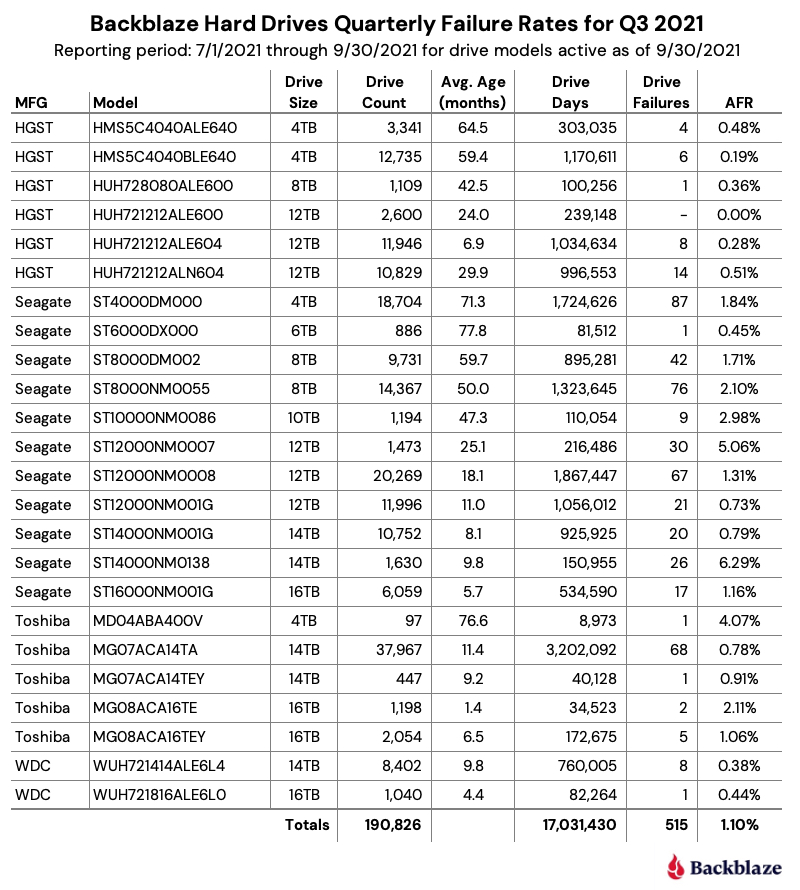
Notes and Observations on the Q3 2021 Stats
The data for all of the drives in our data centers, including the 386 drives not included in the list above, is available for download on the Hard Drive Test Data webpage.
Zero Failures
The only drive model that recorded zero failures during Q2 was the HGST 12TB drive (model: HUH721212ALE600) which is used in our Dell storage servers in our Amsterdam data center.
Honorable Mentions
Five drive models recorded one drive failure during the quarter:
- HGST 12TB drive (model: HUH728080ALE600).
- Seagate 6TB drive (model: ST6000DX000).
- Toshiba 4TB drive (model: MD04ABA400V).
- Toshiba 14TB drive (model: MG07ACA14TEY).
- WDC 16TB drive (model: WUH721816ALE6L0).
While one failure is good, the number of drive days for each of these drives is 100,256 or less for the quarter. This leads to a wide confidence interval for the annualized failure rate (AFR) for these drives. Still, kudos to the Seagate 6TB drives (average age 77.8 months) and Toshiba 4TB drives (average age 75.6 months) as they have been good for a long time.
What’s New
We added a new Toshiba 16TB drive this quarter (model: MG08ACA16TE). There were a couple of early drive failures, but they’ve only been installed a little over a month. This drive is similar to model MG08ACA16TEY, with the difference purportedly being the latter having the Sanitize Instant Erase (SIE) feature, which shouldn’t be in play in our environment. It will be interesting to see how they compare over time.
Outliers
There are two drives in the quarterly results which require additional information beyond the raw numbers presented. Let’s start with the Seagate 12TB drive (model: ST12000NM0007). Back in January of 2020, we noted that these drives were not working optimally in our environment and higher failure rates were predicted. Together with Seagate, we decided to remove these drives from service over the coming months. Covid-19 delayed the project some and the results are the predicted higher failure rates. We expect all of the remaining drives to be removed during Q4.
The second outlier is the Seagate 14TB drive (model: ST14000NM0138). As noted in the Q2 Drive Stats report, these drives, while manufactured by Seagate, were provisioned in Dell storage servers. As noted, both Seagate and Dell were looking into the possible causes for the unexpected failure rate. The limited number of failures, 26 this quarter, have made failure analysis challenging. As we learn more, we will let you know.
HDDs versus SSDs
As a reminder, we use both SSDs and HDDs as boot drives in our storage servers. The workload for a boot drive includes regular reading, writing, and deleting of files (log files typically) along with booting the server when needed. In short, the workload for each type of drive is similar.
In our recent post, “Are SSDs Really More Reliable Than Hard Drives?” we compared the failure rates of our HDD and SSD boot drives using data through Q2 2021. In that post, we found that if we controlled for the average age and drive days for each cohort, we were able to compare failure rates over time.
We’ll continue that comparison, and we have updated the chart below through Q3 2021 to reflect the latest data.
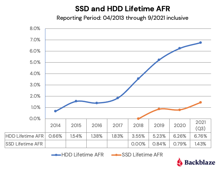
The first four points of each drive type create lines that are very similar, albeit the SSD failures rates are slightly lower. The HDD failure rates began to spike in year five (2018) as the HDD drive fleet started to age. Given what we know about drive failure over time, it is reasonable to assume that the failure rates of the SSDs will rise as they get older. The question to answer is: Will it be higher, lower, or the same? Stay tuned.
Data Storage Changes
Over the last year, we’ve added 40,129 new hard drives. Actually, we installed 67,990 new drives and removed 27,861 old drives. The removed drives included failed drives (1,674) and migrations (26,187). That works out to installing about 187 drives a day, which over the course of the last year, totaled just over 600PB of new data storage.
The following chart breaks down the efforts of our intrepid data center teams.
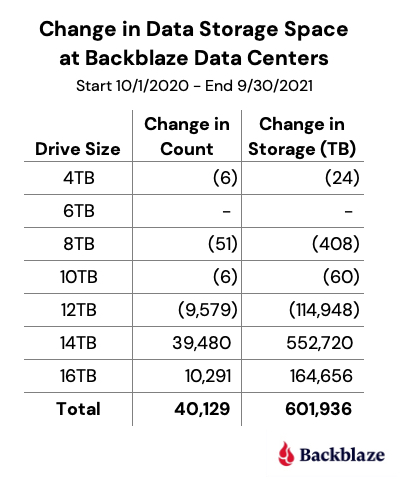
Lifetime Hard Drive Stats
The chart below shows the lifetime AFRs of all the hard drive models in production as of September 30, 2021.

Notes and Observations on the Lifetime Stats
The lifetime AFR for all of the drives in our farm continues to decrease. The 1.43% AFR is the lowest recorded value since we started back in 2013. The drive population spans drive models from 4TB to 16TB and varies in average age from one month (Toshiba 16TB) to over six years (Seagate 6TB).
Our best performing drive models in our environment by drive size are listed in the table below.
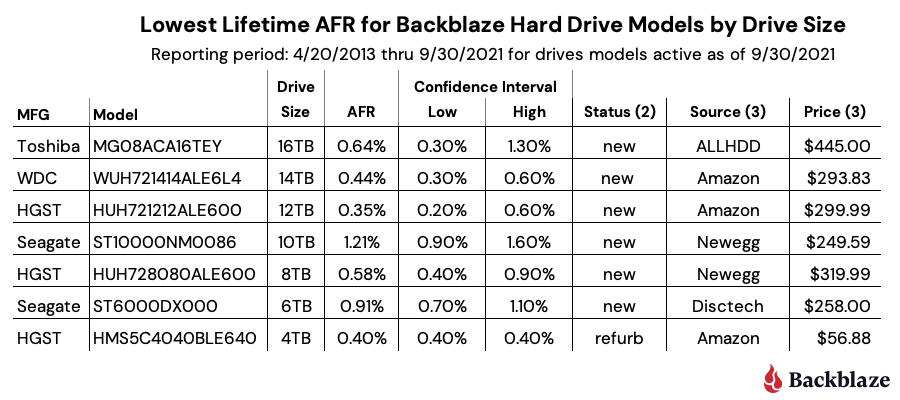
Notes:
- The WDC 16TB drive (model: WUH721816ALE6L0) does not appear to be available in the U.S. through retail channels. It is available in Europe for 549,00 EUR.
- Status is based on what is stated on the website. Further investigation may be required to ensure you are purchasing a new drive versus a refurbished drive marked as new.
- The source and price columns were as of 10/23/2021.
Interested in learning more? Join our webinar on November 4th at 10 a.m. PT with Drive Stats author, Andy Klein, to gain unique and valuable insights into why drives fail, how often they fail, and which models work best in our environment of 190,000+ drives. Register today.
The Hard Drive Stats Data
The complete data set used to create the information used in this review is available on our Hard Drive Test Data page. You can download and use this data for free for your own purpose. All we ask are three things: 1) you cite Backblaze as the source if you use the data, 2) you accept that you are solely responsible for how you use the data, and 3) you do not sell this data to anyone; it is free.
If you just want the summarized data used to create the tables and charts in this blog post, you can download the ZIP file containing the Excel XLXS files for each chart.
Good luck and let us know if you find anything interesting.
The post Backblaze Drive Stats for Q3 2021 appeared first on Backblaze Blog | Cloud Storage & Cloud Backup.
The Chernobyl Exclusion Zone: Ukraine’s Nuclear Eden
Post Syndicated from Geographics original https://www.youtube.com/watch?v=wmo4O_uNA8U