Simulating Amazon EC2 EBS burst credits before downsizing an instance

Post Syndicated from Vineedh George original https://aws.amazon.com/blogs/compute/simulating-amazon-ec2-ebs-burst-credits-before-downsizing-an-instance/

When downsizing an Amazon Elastic Compute Cloud (Amazon EC2) instance, teams often evaluate CPU and memory utilization but overlook the instance’s Amazon Elastic Block Store (Amazon EBS) performance limits for throughput and IOPS. Smaller Amazon EBS-optimized instance types have lower baselines and rely on burst credits to handle peaks. If your workload’s I/O pattern drains those credits faster than the instance can refill them, the instance will throttle your workload to baseline. This post applies to burstable EBS-optimized instances with baselines below their maximum.

This post shows how to pull your instance’s Amazon EBS metrics from Amazon CloudWatch, simulate the burst credit balance against a target instance type’s limits, and help evaluate whether the downsize might be appropriate before making the change.

Solution overview

The analysis compares your workload’s actual I/O pattern against the target instance type’s Amazon EBS limits.

  1. Measure your current Amazon EBS usage. Pull instance-level throughput and IOPS from Amazon CloudWatch at 5-minute granularity. You need at least two weeks of data to capture weekly patterns. Four weeks is better if your workload has monthly cycles. While you pull data, check whether your current instance already hits its Amazon EBS-optimized performance limits.
  2. Compare against the target instance’s limits. Look up the baseline and burst ceiling for your target instance type. Simulate the burst credit balance across your observation window: for each 5-minute interval, calculate whether credits are draining or refilling, and track whether the balance ever hits zero. If it does, you will experience throttling on the smaller instance.
  3. Monitor after the move. Watch InstanceEBSThroughputExceededCheck and InstanceEBSIOPSExceededCheck for immediate throttle detection. Track EBSByteBalance% and EBSIOBalance% to gauge how much headroom remains for workload growth.

Note: These balance metrics are only available on burstable instance sizes where the baseline is lower than the maximum.

Prerequisites

An AWS account with permissions for cloudwatch:GetMetricData and ec2:DescribeInstanceTypes. The instance must be Amazon EBS-optimized (AWS enables EBS-optimization by default on most current-generation instance types).

Note: AWS doesn’t provide these instance-level Amazon CloudWatch metrics in AWS Outposts, AWS Local Zones, or AWS Wavelength Zones.

Pulling instance-level Amazon EBS metrics from Amazon CloudWatch

Amazon CloudWatch provides Amazon EBS metrics at the instance level in the AWS/EC2 namespace, using the InstanceId dimension. Here are the metrics that you need:

Metric What it measures
EBSReadBytes Total read bytes in the period
EBSWriteBytes Total write bytes in the period
EBSReadOps Total read operations in the period
EBSWriteOps Total write operations in the period
EBSIOBalance% IOPS burst credit balance (0-100%)
EBSByteBalance% Throughput burst credit balance (0-100%)
InstanceEBSIOPSExceededCheck 1 if instance hit IOPS limit, 0 otherwise
InstanceEBSThroughputExceededCheck 1 if instance hit throughput limit, 0 otherwise

The first four metrics are the inputs for the simulation. The rest are useful context:

  • EBSIOBalance% and EBSByteBalance% show how much of the burst credit pool remains, as a percentage. On the current (larger) instance, these should sit at or near 100 percent. If they’re dipping, the workload is already consuming burst credits at the current size, and a downsize will make it worse.

Note: These metrics only appear on instances where the baseline is lower than the maximum.

  • InstanceEBSIOPSExceededCheck and InstanceEBSThroughputExceededCheck are binary: 1 means the instance hit its EBS-optimized performance limit within the last minute. If either is firing on the current instance, the workload is already throttling and should be addressed before considering a downsize.

Pull these at 5-minute granularity for at least two weeks (four if your workload has monthly cycles). Amazon CloudWatch retains 5-minute data points for 63 days, so that’s your upper bound. You can retrieve the data through the AWS Command Line Interface (AWS CLI) (GetMetricData API), the Amazon CloudWatch console, or any AWS SDK. The metrics live in the AWS/EC2 namespace with your InstanceId as the dimension.

Use the Maximum statistic for the four I/O metrics and Minimum for the balance percentages. Maximum captures the highest 1-minute data point within each 5-minute window, which is the conservative choice for the simulation inputs. The Sum statistic gives a more precise total for each interval, but Maximum is the intentionally conservative choice. It assumes the peak 1-minute rate held for the full 5-minute window, which overstates actual consumption. Minimum on the balance metrics captures the lowest point the balance hit within each window, so you see the actual dips rather than averaging them away. For the ExceededCheck metrics, use Maximum (you want to know if the limit was hit at any point in the window).

Combine read and write values to get totals per interval. To convert to per-second rates:

total_throughput_MBps = (EBSReadBytes + EBSWriteBytes) / (60 * 1024 * 1024)
total_iops            = (EBSReadOps + EBSWriteOps) / 60

The division by 60 (not by the period length) is intentional. The Maximum statistic for a 5-minute period returns the highest 1-minute aggregate within that window, not a 5-minute total. Dividing by 60 converts that 1-minute peak to a per-second rate. The additional divisions by 1,024 convert bytes to mebibytes to match the units in describe-instance-types.

Comparing actual usage against target limits

From the Amazon EBS-optimized instances documentation, find the baseline and maximum (burst ceiling) for both IOPS and throughput on your target instance type. You can also pull these programmatically:

aws ec2 describe-instance-types \
  --instance-types r8i.large \
  --query 'InstanceTypes[0].EbsInfo.EbsOptimizedInfo' \
  --output table

This returns the baseline and maximum bandwidth (MB/s) and IOPS for the instance type. Note that BandwidthInMbps is megabits per second (network-style units), while ThroughputInMBps is megabytes per second. The throughput values are what you compare against your Amazon CloudWatch data.

-------------------------------------------
|          EbsOptimizedInfo               |
+----------------------------+------------+
| BaselineBandwidthInMbps    | 650        |
| BaselineThroughputInMBps   | 81.25      |
| BaselineIops               | 3600       |
| MaximumBandwidthInMbps     | 10000      |
| MaximumThroughputInMBps    | 1250.0     |
| MaximumIops                | 40000      |
+----------------------------+------------+

BaselineThroughputInMBps is the sustained rate the instance can deliver indefinitely. MaximumThroughputInMBps is the burst ceiling, the absolute maximum the instance can deliver while it has burst credits. Same relationship for IOPS. IOPS and throughput have separate burst budgets, tracked by EBSIOBalance% and EBSByteBalance% respectively.

How burst credits work

The instance maintains a credit pool for each budget (IOPS and throughput). The pool capacity is:

credit_pool = (burst_ceiling - baseline) * 1800

The 1800 comes from 30 minutes (1800 seconds) of burst at the maximum rate, which AWS provisions as the pool size for burstable Amazon EBS-optimized instances. Credits drain when usage exceeds baseline and refill when usage is below baseline, at a rate of baseline – effective_usage per second, where effective_usage is min(actual_usage, burst_ceiling). The instance cannot deliver more than the ceiling regardless of credit balance, so credits drain at the ceiling rate, not the requested rate. The pool is capped at its maximum and floored at zero. When credits hit zero, your workload is throttled to baseline performance. AWS resets the pool to full every 24 hours, giving you at least 30 minutes of burst capacity per day.

See Improving application performance and reducing costs with Amazon EBS-optimized instance burst capability for a detailed walkthrough of how burst credits work.

Simulating the credit balance

With the time series data and the target limits, you can simulate what the credit balance would look like on the smaller instance. For each 5-minute interval in your observation window:

effective_usage = min(actual_usage, burst_ceiling)
net_credit_change = (baseline - effective_usage) * interval_seconds
new_balance = previous_balance + net_credit_change
new_balance = clamp(new_balance, 0, credit_pool)

Where interval_seconds is 300 for 5-minute data or 60 for 1-minute data.

When actual usage is below baseline, credits accumulate. When above, they drain. Run this across the full observation window, resetting the pool to full at the start of each 24-hour period to model the AWS top-off guarantee. Start each day with a full pool, then drain and refill through the day’s intervals. If the balance hits zero on any day, the workload will throttle on the smaller instance.

Run the simulation twice: once for IOPS, once for throughput. Throttling happens if either pool hits zero.

A Python script that pulls Amazon CloudWatch data for a given instance ID, looks up the target instance type’s Amazon EBS limits, and runs this simulation end-to-end is available at sample-ec2-ebs-burst-analyzer repository.

This simulation is an approximation

It models credit behavior at 5-minute (or 1-minute) granularity using Amazon CloudWatch aggregates, not the actual per-second I/O stream. Two factors make the simulation more conservative than reality, and two can make reality worse than the simulation.

The Maximum statistic returns the highest 1-minute total within each 5-minute window. The simulation applies that peak rate across the full 300-second interval. This overestimates credit drain by up to 5x for any given interval, because the other 4 minutes likely had lower usage. The tradeoff is intentional. If the simulation says the workload fits, the result is reliable. If it says the workload doesn’t fit, the actual situation might be better than predicted. In that case, re-run with the Average statistic for a less conservative check, or pull 1-minute data (available for the most recent 15 days in Amazon CloudWatch) for higher fidelity.

Working in the other direction, two things can make the real situation worse than the simulation predicts. If the downsize also reduces memory, database workloads (SQL Server buffer pool, PostgreSQL shared_buffers, Oracle SGA) will generate more disk I/O than what you measured because the smaller cache forces more page reads from Amazon EBS. Account for this by including additional headroom in the burst credit budget. And I/O spikes that last milliseconds don’t show up in 5-minute Amazon CloudWatch data. If EBSByteBalance% or EBSIOBalance% are trending down on the current instance but your throughput metrics look fine, the workload is microbursting.

What to look for in the results

The simulation produces two outputs per budget (IOPS and throughput): the low-water mark (lowest credit balance across the observation window) and the number of intervals where the balance hit zero.

  • IOPS credit balance (EBSIOBalance%) – If the simulated low-water mark stays well above zero, the workload’s IOPS pattern fits within the target’s burst budget. A low-water mark of 90 percent means the workload barely touches the IOPS burst pool. A low-water mark of 40 percent means it fits today but has limited room for IOPS growth.
  • Throughput credit balance (EBSByteBalance%) – Same logic for throughput. Check this independently because a workload can be comfortable on IOPS but tight on throughput, or the reverse.
  • Intervals at zero – If either balance hits zero on any day, the workload will throttle to baseline on this instance type.
  • Peak usage vs. burst ceiling – The ceiling is the absolute maximum regardless of credit balance. If your peak throughput exceeds MaximumThroughputInMBps or peak IOPS exceeds MaximumIops, the instance will cap I/O at the ceiling rate during those intervals. This doesn’t mean the workload doesn’t fit overall (credits might still be fine), but the application will experience reduced I/O during those peaks. A handful of brief spikes may be acceptable. Sustained ceiling breaches are a stronger signal to size up.
  • Throttled intervals – The most direct measure of impact. A throttled interval is one where the credit balance is at zero and usage exceeds baseline. During these intervals, the instance cannot deliver what the workload is asking for. A few throttled intervals during a nightly batch may be tolerable. Dozens per day during business hours is a problem.

The following two figures show what these outcomes look like. In the first, the workload bursts above baseline during business hours but credits never fully deplete. The minimum balance stays at 82 percent, well above zero. This workload is safe to downsize.

Figure 1: Chart showing observed IOPS over 24 hours with baseline and ceiling reference lines. IOPS bursts above baseline during business hours. Simulated credit balance dips to a minimum of 82% and recovers, indicating the workload sustains burst credits on this instance type.

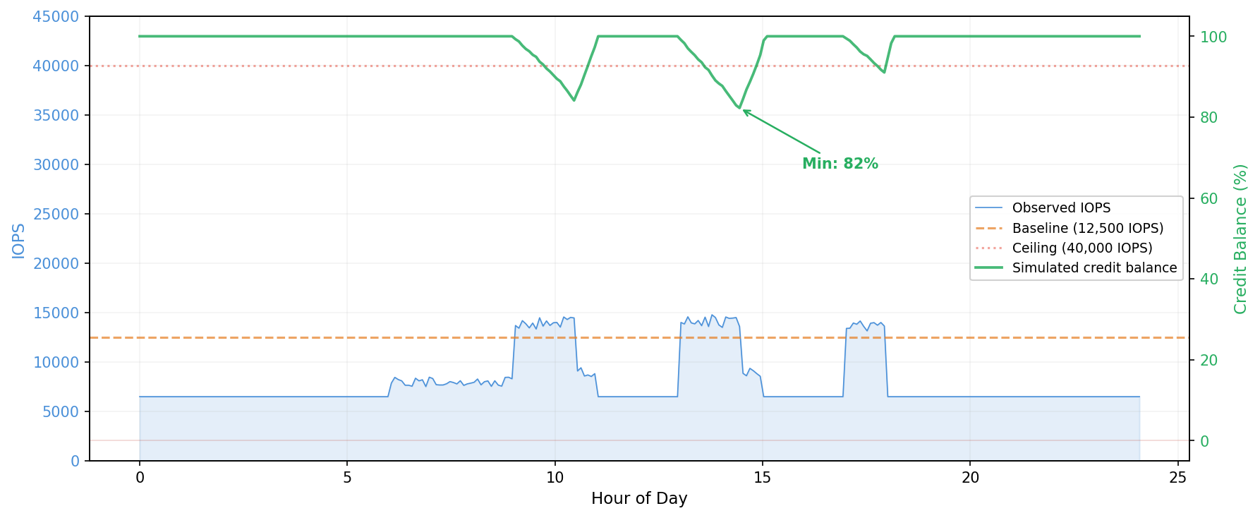
Figure 1: Amazon EC2 EBS-optimized instance burst credit simulation: credits sustained

In the second figure, the same workload runs on a smaller instance type with a lower burst pool. Credits deplete within the first burst window and stay near zero for most of the business day. This workload would throttle on the smaller instance.

Figure 2: Chart showing the same IOPS pattern with a smaller burst pool. Simulated credit balance drops to 0% during each burst window, indicating burst credits are depleted and the workload would be throttled on this instance type.

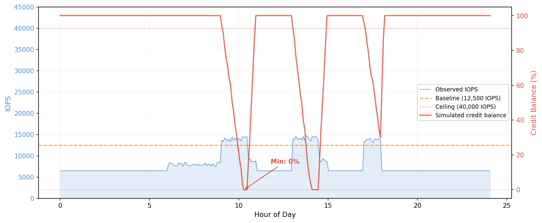
Figure 2: Amazon EC2 EBS-optimized instance burst credit simulation: credits depleted

Worked examples

The following servers are from a customer running SQL Server on EC2. We simulated the burst credit balance for each against the proposed target instance type, using 28 days of Amazon CloudWatch data at 5-minute granularity with the Maximum statistic.

Server A: fits comfortably (current: c6in.4xlarge; proposed: r6i.large)

Target limits: baseline 3,600 IOPS / 81.25 MB/s, burst ceiling 40,000 IOPS / 1,250 MB/s.

Simulating the credit balance across 28 days with a daily pool reset:

IOPS Throughput
Credit pool 65,520,000 2,103,750 MB
Low-water mark 52,084,325 (79.5%) 1,656,415 MB (78.7%)
Intervals at zero 0 0

On the worst day for throughput, here’s what the simulation looks like during the evening burst window, showing how credits drain and recover interval by interval:

Time Throughput (MB/s) Net credit change Balance Balance %
22:00 154.25 -21,900 1,854,076 88.1%
22:05 22.57 +17,603 1,871,679 89.0%
22:10 452.16 -111,273 1,760,406 83.7%
22:15 427.89 -103,991 1,656,415 78.7%
22:20 30.99 +15,077 1,671,492 79.5%

At 22:10 and 22:15, throughput spiked above 400 MB/s, well above the 81.25 MB/s baseline but still under the 1,250 MB/s burst ceiling. Each interval drained roughly 100,000 credits. The pool hit its low-water mark of 78.7 percent at 22:15, then immediately began recovering as throughput dropped. By 23:55, the pool was back to 100 percent.

Assessment: fits, with roughly 20 percent headroom on the worst day.

Server B: fits but tight (same workload as Server A; proposed: r5.large)

Target limits: baseline 3,600 IOPS / 81.25 MB/s, burst ceiling 18,750 IOPS / 593.75 MB/s.

IOPS Throughput
Credit pool 27,270,000 922,500 MB
Low-water mark 13,834,325 (50.7%) 475,165 MB (51.5%)
Intervals at zero 0 0

Same workload, same burst pattern, but the r5.large has a smaller credit pool, so the same spikes drain a larger percentage. The throughput low-water mark drops from 78.7 percent to 51.5 percent. The same evening burst window that used 20 percent of the r6i.large pool now consumes nearly half the r5.large pool:

Time Throughput (MB/s) Net credit change Balance Balance %
22:00 154.25 -21,900 672,826 72.9%
22:05 22.57 +17,603 690,429 74.8%
22:10 452.16 -111,273 579,156 62.8%
22:15 427.89 -103,991 475,165 51.5%
22:20 30.99 +15,077 490,242 53.1%

This still fits, but with limited margin. Any workload growth (more users, larger databases, additional backup jobs) could push the balance toward zero. Separately, a single IOPS interval reached 20,226, exceeding the r5.large burst ceiling of 18,750. The instance can only deliver up to the ceiling while credits remain, so the application received 18,750 IOPS during that interval. That single spike would not cause sustained throttling, but combined with the tight throughput margins, it confirms this workload is at the boundary of what r5.large can handle.

Assessment: fits today, but not a safe long-term choice.

Server C: ceiling breach (current: c6in.4xlarge; proposed: r6i.xlarge)

Target limits: baseline 6,000 IOPS / 156.25 MB/s, burst ceiling 40,000 IOPS / 1,250 MB/s.

Peak throughput: 1,502.94 MB/s. This exceeds the 1,250 MB/s burst ceiling. During those peak intervals, the instance would cap throughput at 1,250 MB/s while credits remain. If credits are exhausted, throughput drops to the 156.25 MB/s baseline. The credit simulation might still show the workload fits (credits never hit zero), but the application would experience reduced I/O during those peaks. For this customer, the peaks coincided with production SQL Server activity, so even brief throttling wasn’t acceptable, and a larger instance type was needed.

Assessment: workload will be throttled during peak intervals. Whether that’s acceptable depends on the application’s sensitivity to I/O latency.

Monitoring after the resize

The pre-migration analysis uses historical data from the larger instance. After you resize, real metrics replace the simulation. Monitor the following three layers:

  1. InstanceEBSThroughputExceededCheck and InstanceEBSIOPSExceededCheck = 1 means the instance is actively throttling. This is the definitive signal. Alarm on Sum > 0 over 3 consecutive 1-minute periods to filter out single-second spikes that resolve on their own.
  2. EBSByteBalance% and EBSIOBalance% trending downward over days or weeks means the workload is growing into the instance’s limits. You’re not throttling yet, but you’re on a trajectory. An instance that dips to 90 percent nightly and recovers is in a different position than one that dips to 40 percent and barely recovers before the next burst. Neither instance is throttling, but the first has headroom while the second doesn’t.
  3. EBSByteBalance% and EBSIOBalance% stay at 100 percent means the workload never exceeds baseline. The instance has unused capacity, and you might even be able to go smaller.

If the workload has weekly patterns, allow at least one full week of data before drawing conclusions.

Conclusion

In this post, we showed how to simulate the EBS-optimized instance burst credit balance against a target instance type’s limits before downsizing an Amazon EC2 instance. The approach pulls Amazon CloudWatch metrics at 5-minute granularity, compares actual throughput and IOPS against the target’s baseline and burst ceiling, and tracks whether the credit balance would hit zero during the observation window.

This covers the Amazon EBS dimension of a right-sizing decision. A complete evaluation also considers CPU utilization, memory usage, and network throughput against the target instance’s limits. For workloads where Amazon EBS utilization is well below baseline, the burst credit simulation might not be necessary.

To run this analysis on your own instances, see the companion script in the sample-ec2-ebs-burst-analyzer repository. For more on how instance-level burst credits work, see Improving application performance and reducing costs with Amazon EBS-optimized instance burst capability. For instance-level EBS baseline and burst limits by instance type, see Amazon EBS-optimized instances.

FairScan 2.0 released

Post Syndicated from jzb original https://lwn.net/Articles/1078242/

Version
2.0
of the FairScan document-scanning app for Android has been
released. The headline feature for this release is the addition of
optical-character-recognition (OCR) support using Tesseract to produce PDFs
with searchable text from scans. FairScan developer Pierre-Yves
Nicolas has written a detailed
blog
about adding the feature and explaining why it had not been added
previously.

That looks nice, so why didn’t FairScan have it before? That’s
because FairScan wasn’t ready for it: I wouldn’t be comfortable if
FairScan was giving you wrong text half of the time. To get good
results from an OCR engine, you need to provide it a readable
image. If it’s hard to read for a human, it’s certainly also hard to
read for an OCR engine.

Over the past year, I worked on different parts of FairScan’s
automatic processing to transform photos of documents into PDFs that
are easy for humans to read:

  • document detection
  • perspective correction
  • shadow reduction
  • brightness and contrast enhancement

All this work on image processing helped FairScan produce clean
PDFs and can now also contribute to making text recognition effective.

FairScan is available via Google
Play
or F-Droid.

Security updates for Wednesday

Post Syndicated from jzb original https://lwn.net/Articles/1078339/

Security updates have been issued by AlmaLinux (hplip, kernel, kernel-rt, libpng12, libpng15, libxml2, libxslt, mysql:8.0, mysql:8.4, opencryptoki, openssl, postfix, postgresql:15, rsync, and webkit2gtk3), Debian (asterisk, atril, gsasl, and libreoffice), Fedora (ack, bird, chromium, firefox, ldns, librabbitmq, nextcloud, nss, openslide, perl-Protocol-HTTP2, tig, vorbis-tools, and xen), Mageia (coturn, log4cxx, and python-tornado), SUSE (389-ds, buildah, container-suseconnect, distribution, editorconfig-core-c, elemental-system-agent, glib-networking, google-guest-agent, google-osconfig-agent, kernel, libcaca, libXpm, opensc, openssl-3, openvswitch, perl-Crypt-PBKDF2, python-python-dotenv, python311-aiosmtplib, python311-zeroconf, runc, shim, and sqlite3), and Ubuntu (ca-certificates, keystone, librabbitmq, linux, linux-aws, linux-kvm, linux-aws-hwe, linux-azure, linux-gcp, linux-hwe, linux-oracle, linux-azure, linux-azure, linux-gcp, linux-hwe, linux-oracle, linux-azure-6.8, linux-oracle-5.15, nova, openimageio, qemu, and squid).

Introducing the Cloudflare One stack: agent-powered deployment

Post Syndicated from AJ Gerstenhaber original https://blog.cloudflare.com/cloudflare-one-stack/

Adopting or migrating to a Zero Trust network architecture can be a daunting task. Before a single policy changes, teams have to recall how their network is actually built: which applications exist, their authentication and authorization constructs, how traffic flows between them, and any assumptions the current architecture makes. This hands-on process requires practitioners to decode the intent behind every security and routing policy in place.

Today, we’re releasing the Cloudflare One stack, a set of skills you give to your agent to configure, deploy, and manage your Zero Trust environment for you. This toolkit is designed to help automate the process of learning an entirely new security suite and mapping your existing one into Cloudflare.

Cloudflare has worked with thousands of customers through exactly this process. That repetition built expertise on where migrations stall, what questions come up every time, and what it takes to move forward. The Cloudflare One stack packages that expertise and makes it more accessible than ever. 

The agent gap in network security

Teams are already using agents to write code, triage alerts, and automate workflows. Organizations are increasingly asking for Cloudflare-provided tooling to help agents execute on security workflows. On their own, agents are not trained on the nuances of an organization’s specific network topology or vendor configurations.

By providing prescriptive and authoritative guidance, organizations can layer this context into their existing toolkit to make better use of the security products they are already deploying.

Cloudflare has long been the easiest-to-deploy SASE vendor in the market. The stack extends that philosophy to agents: it gives them the context, tools, and structured reasoning they need to operate on your security infrastructure.

What is the Cloudflare One stack?

The Cloudflare One stack is a collection of skills that can be used with any agent. As with any skill, you can use them standalone, layer in your own context, or build tooling on top. It was purpose-built to help security practitioners across the entire lifecycle of evaluating, deploying, and managing Cloudflare One.

The stack was built by synthesizing hand-curated knowledge from employees with tens of thousands of hours of experience working with customers on Cloudflare One products. It contains tools for planning, managing, and implementing your user and agent security infrastructure on Cloudflare. It also contains handpicked logic for migrating from legacy vendors like Zscaler and Palo Alto Networks.

When used in conjunction with the Cloudflare code mode MCP server, the stack gives agents a typed interface to the Cloudflare API. Agents can query your live account, inspect configurations, and make changes through a curated set of Cloudflare-recommended workflows rather than ad-hoc API calls.

What’s in the stack?

The Cloudflare One stack ships as two lightweight skill files: cloudflare-one and cloudflare-one-migration. Together they cover migrating to, building an implementation for, managing, and troubleshooting your Cloudflare One deployment:

  • Remote access and VPN replacement with Cloudflare Access

  • User, network, device, and data security with Cloudflare Gateway

  • Connectivity with Cloudflare Tunnel, Cloudflare Mesh, and Cloudflare WAN

  • Migration guidance with explicit detail for moving from other SASE vendors

  • Network diagram interpretation and generation, so you can visualize proposed changes to your network in a way that is easy for you and your team to understand

  • Vendor concept translation, which maps concepts between SASE vendors to reduce the barrier to evaluating and switching providers

  • Troubleshooting and operations, with the Digital Experience Monitoring (DEX) toolkit and automated rule recommendations

How it works

The stack is available in the Cloudflare Skills repository. Each skill file contains structured knowledge, decision trees, and tool definitions that agents load automatically when the context matches. Give this to your agent and let it help you set up, configure, and manage your Zero Trust environment:

The cloudflare-one skill covers general product guidance. For example, if you ask an agent for the best way to replace your VPN infrastructure with Cloudflare Tunnel or Cloudflare Mesh, the skill knows how to:

  1. Inventory your existing VPN applications and identify which connectivity model each requires

  2. Map each application to the appropriate Cloudflare primitive — self-hosted Access application, Tunnel-connected service, or Mesh-connected network segment

  3. Generate a recommended deployment sequence that minimizes disruption during cutover

  4. Produce a configuration summary your team can review before making any changes

The cloudflare-one-migration skill covers vendor-to-vendor translation. For example, if you ask an agent to migrate your Zscaler Private Access applications to Cloudflare Access, the skill knows how to:

  1. Map Zscaler application definitions to Cloudflare Access application definitions

  2. Transform Zscaler user groups and policies into Cloudflare Access policies

  3. Use the Cloudflare API to create the equivalent resources in your account

  4. Generate a summary of what was migrated and what requires manual review

The migration logic in the stack is the same logic used in Cloudflare’s Descaler and Deskope programs. Those programs have already moved enterprise customers from Zscaler and Netskope to Cloudflare One in hours rather than months. The stack makes that capability available to any customer or partner, at any time, without waiting for a scheduled engagement.

More ways to use the stack

The Cloudflare One stack can also:

  • Recommend security rules based on traffic seen in your live account

  • Automatically migrate your existing Zscaler Private Access applications into self-hosted Cloudflare Access applications

  • Investigate anomalies in your secure web gateway HTTP logs and build rules to resolve issues users are seeing

  • Report on user stability with the DEX toolkit and take actions to improve user latency in key scenarios

Whether you are loading the skill from an agent or building custom tooling on top, the Cloudflare One stack handles all of these use cases and more.

For partners, too

While this simplifies ongoing management for customers who have already adopted the Cloudflare One product suite, it is also a tool for the Cloudflare partner network. Partners can use it to help their customers deploy faster, manage more effectively, troubleshoot with increased accuracy, and drive issues to resolution.

What’s next

You can start using the Cloudflare One stack today. To get the most out of the stack, pair it with the Cloudflare code mode MCP server. The MCP server gives your agent live access to the Cloudflare API through a single, compressed interface that keeps authentication credentials out of the model context. 

The Cloudflare One stack will continue to expand as Cloudflare One products evolve. New skills for additional migration sources and more advanced troubleshooting workflows are already in development.

As we learn more about how customers and partners utilize these skills files, we plan to build more robust tooling around these skills. If you are a customer or partner and want to share feedback on what the stack should handle next, reach out through your account team or open an issue in the repository.

Големият отсъстващ. Детските палиативни грижи в публичните политики и в публичния дебат

Post Syndicated from Надежда Цекулова original https://www.toest.bg/golemiyat-otsustvasht-detskite-paliativni-grizhi-v-publichnite-politiki-i-v-publichniya-debat/

Големият отсъстващ. Детските палиативни грижи в публичните политики и в публичния дебат

Кое е първо – кокошката или яйцето? В контекста на настоящата поредица този въпрос звучи така: кое е първо – качествените публични политики за детски палиативни грижи или качественият разговор и разбирането по темата? 

В момента в България липсват и двете. Омагьосаният кръг се затваря, от една страна, от нормативна рамка, в която детските палиативни грижи се споменават инцидентно и свенливо, и от друга – от публично говорене, в което понятието съществува, но е изпразнено от съдържание. 

А като не говорим за качеството на живот на децата с тежки диагнози, сме по-склонни да забравяме за тях и семействата им.


Съвременните палиативни грижи не са „медицински грижи в края на живота“, както все още често се смята в България, а комплексен подход, чиято роля е да направи живота на хората с тежко заболяване по-хубав, каквато и да е неговата продължителност. 

Според актуалната дефиниция на Световната здравна организация палиативните грижи включват набор от услуги от редица професионалисти – лекари, медицински сестри, психолози, социални работници, парамедици, фармацевти, рехабилитатори, духовни лица, дори доброволци. Всички те са еднакво важни и имат роля в подкрепата както на пациента, така и на неговото семейство. Да, част от работата им е да облекчават болката и клиничните симптоми. Но също и да се грижат за психологическата подкрепа, за решаването на казусите от всекидневието и дори за дреболии като това кой ще сготви днес и кой ще заведе здравото дете в семейството на футбол например. 

Фокусът на палиативните грижи такива, каквито ги разбира съвременната грижа за деца със съкращаващи живота заболявания и състояния, е какво може да се направи, за да живеят тези деца и семействата им възможно най-нормално и да имат в живота си всички достъпни за състоянието им възможности да изпитват радост.

Детските палиативни грижи в публичните политики

Да има „публична политика“ за детските палиативни грижи означава да има ред, по който всяко дете, нуждаещо се от такива грижи, и неговото семейство да могат да ги получат навременно и с гарантирано качество. В момента в България има редица дефицити, заради които можем с чиста съвест да кажем, че публични политики в сферата липсват. Подробна аргументация на това твърдение може да се намери в правния анализ на адв. Мария Шаркова в доклада „Готови ли сме за детски хоспис в България“, публикуван от „Ида – фондация за палиативни грижи за деца“. 

Юристката посочва, че сред най-сериозните дефицити в законодателството е рамката, според която палиативните грижи включват само медицински дейности, извършвани в болници, и то на пациенти в терминален стадий. Това лишава от грижи много пациенти, които са подходящи за палиативни грижи, но не са в терминален стадий, се обяснява в анализа. 

Освен това, както се е случвало неведнъж и в други сфери, палиативните грижи за деца, оказва се, на хартия могат да бъдат извършвани и в дома на детето. На практика обаче нито е регламентиран ред как това да се прави, нито е определено финансиране за самата грижа или за специфични апарати, медицински изделия и други средства, които да подпомогнат близките в грижата за детето (например кислородни концентратори, апарати за аспирация и др.). Медицинското образование също не включва достатъчна подготовка по темата, а в българската номенклатура на медицинските специалности липсва такава по палиативни грижи (и в частност – палиативни грижи за деца).

Просто добави радост. Какво са съвременните палиативни грижи за деца
Разполагаме със здравна система, която все още не успява да се пречупи така, че да осигури детство там, където заболяването е отнело почти всичко друго. Как изглеждат детските палиативни грижи в България? Първи текст от новата поредица на Надежда Цекулова за детските палиативни грижи.
Големият отсъстващ. Детските палиативни грижи в публичните политики и в публичния дебат

В нормативните документи на българското Министерство на здравеопазването за грижа за деца с тежки увреждания или хронични заболявания се говори за комплексно обслужване. То се осигурява в специално създадени Центрове за комплексно обслужване на деца с увреждания и хронични заболявания, които ще срещнете навсякъде като ЦКОДУХЗ. Много от тези центрове се създават на мястото на закритите домове за деца с увреждания от времената на социализма, като идеята им на хартия е да предоставят различен, по-съвременен и хуманен модел на грижа. 

„Комплексното обслужване“ кореспондира с английския термин complex care (комплексни грижи). Разликата между palliative care и complex care обаче сама по себе си е голяма, а между „комплексно обслужване“ и „палиативни грижи“ нараства допълнително.

В англоезичния си вариант терминът „комплексни грижи“ обхваща целия набор мултидисциплинарни медицински грижи за хора с тежки и хронични страдания и се отнася до откликването на различните нужди, които специфичното състояние изисква. 

Палиативните грижи от своя страна са свързани с начините да бъде повишено качеството на живота на болното дете и семейството му. Замяната на „грижа“ с „обслужване“ в българското наименование допълнително дехуманизира децата, които имат нужда от тази грижа. Наред с това в ЦКОДУХЗ въобще не е предвидена възможност за присъствие на близките, а само стаи за срещи, и то при спазване на строги правила. 

В какъв смисъл „качество на живот“?

Това състояние на публичните политики означава, че макар да се търсят варианти да бъдат посрещнати физическите нужди на едно дете с тежки проблеми, не се търсят отговори на въпросите за качеството на живота – и неговия, и на семейството му. Иначе казано, 

някъде по света съществуват системи, които се занимават не само с това дали едно болно дете е нахранено, преобуто и медикирано, а се интересуват дали и доколко то успява да живее щастливо със своето семейство. 

Една от причините този въпрос да не е засегнат в публичните политики е, че той изобщо много рядко ни хрумва. Родители, минали през това, споделят, че усещат определено очакване на обществото от тях – сякаш ако в едно семейство има тежко болно дете, и то, и близките му са длъжни да са страдащи и угрижени денонощно и без почивка. Това субективно усещане се потвърждава и при по-системно наблюдение на начина, по който се говори публично по темата.

Анализ на публикации, включващи понятието „детски палиативни грижи“, показва, че идеята, че тежко болните деца и семействата им трябва да имат качествен живот, напълно липсва от публичния ни наратив. Проучването обхваща 180 публикации в български дигитални медии в периода 2023–2024 г. и е изготвенo с подкрепата на Нов български университет и Медийна агенция „Персептика“.

От анализа става ясно, че езикът и съдържанието, описващи качеството на живот на едно дете, практически липсват в публикациите, свързани с детските палиативни грижи, както липсват и ключовите хора в разказа на една такава история. 

КОЙ говори за детските палиативни грижи в България?

Големият отсъстващ. Детските палиативни грижи в публичните политики и в публичния дебат

По данни на медийна агенция „Персептика“ в дигиталните медии в България за две години са публикувани 180 материала, в които става дума за детски палиативни грижи. Най-голям интерес към темата са показали специализираните уебсайтове за здравна информация (45 публикации) и дигиталните информационни медии с национален профил (43 публикации). В сайтовете на трите национални телевизии има общо две публикации по темата – по една в БНТ и Нова телевизия, и нито една в bTV.

Електронните медии с национален обхват продължават да играят важна роля в информираността на широката аудитория в България както през уебсайтовете си, така и чрез ефирните си програми и затова липсата на интерес у тях по темата означава и ниско познаване от аудиторията им. В същото време националните телевизии и радиостанции имат не само по-широка аудитория, но и нормативно определени задължения за отразяване на обществено значими теми, особено когато са свързани с уязвими групи, като тежко болни деца и техните семейства.

Анализът на говорителите, присъстващи в публикациите по темата за детските палиативни грижи, показва, че най-често това са медицински специалисти – лекари, свързани с педиатричната грижа и системата на общественото здраве (д-р Благомир Здравков, д-р Бояна Петкова, проф. Иван Литвиненко са най-често срещаните имена), които представят темата от гледна точка на клиничните нужди, липсата на структурирани услуги и необходимостта от системно решение. 

Значително е и участието на експерти по медицинско и здравно право (адв. Мария Шаркова), граждански активисти и др. Приблизително в 47% от публикациите (85 бр.) са цитирани говорители, свързани с една гражданска организация – „Ида – фондация за палиативни грижи за деца“, в други 25% (45 бр.) са цитирани лекари от СБАЛДБ „Проф. д-р Иван Митев“ и в още 14,4% (26 бр.) – министри на здравеопазването и на труда и социалната политика. На практика се вижда, че публичният разказ се създава от една гражданска инициатива и една болница, което отново говори за липса на системност и широк дебат.

КАК се говори за детските палиативни грижи в България?

Често срещани думи в изследваните публикации

Среща ли се в публикацията следната дума или нейна производна

Брой публикации, в които се открива думата

Болница

139

Семейство

78

Терминално

51

Смърт

34

Умиращ

17

Приятели

16

Достойнство

13

Учене

9

Радост

3

Игра

0

Проследяването на ключовите думи в изследваните публикации сочи, че понятието „детски палиативни грижи“ почти винаги върви ръка за ръка с понятието „болница“, а в около половината от случаите – и с производни на думата „смърт“. За сметка на това обаче липсват думи, които биха описали качеството на живот на децата и техните семейства, каквито са например „учене“, „игра“ и „радост“.

Как да говорим за деца с тежки заболявания. Право, етика и човечност
Публичният разговор за тежко болните деца често се движи между две крайности – патетична жалост и почти пълно мълчание. Там някъде са и самите деца и семействата им. Как да се говори за страдание, без то да се превръща в сюжет? От Надежда Цекулова.
Големият отсъстващ. Детските палиативни грижи в публичните политики и в публичния дебат

Липсва и етично обоснован личен и емоционално ангажиран език за смъртта. Децата, за които се говори, не са личности с преживявания и собствен глас, а абстрактни фигури. Това лишава разговора за детските палиативни грижи от хуманност, а именно хуманността е в сърцевината на съвременното разбиране за този тип грижи. Сравнително честото присъствие на думата „семейство“ (в 78 публикации), съчетано с пълна липса на родители или братя и сестри като реални говорители в публикациите, разкрива интересен парадокс. 

Сходно е положението с думата „приятели“. Формално тя се среща в 16 публикации, но съдържателният ѝ анализ показва, че социалната среда на детето – извън семейството – практически отсъства от медийния разказ за палиативните грижи. 

Въпросът с „достойнството“ на децата, нуждаещи се от палиативни грижи, също остава необговорен – думата присъства, но в нито една публикация не се коментира какво на практика означава за едно тежко болно дете и семейството му да живеят „с достойнство“.

Първо политиките или първо разказът?

Изследвания сочат, че начинът, по който говорим по дадена тема, може да промени много – да ни научи, да ни преведе през чужди истории, да променя закони и нагласи. И ако в публичния разговор за „палиативни грижи“ се обсъжда „качество на живота“, „радост“ и „игра“, вместо „болница“ и „смърт“, ако историите се разказват от главните им герои, това ново послание рано или късно ще достигне до правилните си адресати. 

А дотогава думите, които избираме да не включим в този разговор, всъщност ще са думите, които показват в коя посока сме решили да гледаме като общество и какво остава извън полезрението ни.


Големият отсъстващ. Детските палиативни грижи в публичните политики и в публичния дебат

Настоящата публикация е създадена по проект „Да говорим с грижа: Палиативните грижи за деца през погледа на медиите“. Проектът се осъществява благодарение на най-голямата социално отговорна инициатива на Лидл България „Ти и Lidl“, в партньорство с Фондация „Работилница за граждански инициативи“, Български дарителски форум и Асоциация на европейските журналисти. Отговорността за съдържанието е на журналистката Надежда Цекулова и по никакъв начин не отразява официалните позиции на финансиращите организации.

Големият отсъстващ. Детските палиативни грижи в публичните политики и в публичния дебат

Malware à la Mode: Tracking Dropping Elephant Tradecraft Through a China-Themed Loader Chain

Post Syndicated from Anna Širokova original https://www.rapid7.com/blog/post/tr-malware-tracking-dropping-elephant-tradecraft-china-themed-loader-chain

Executive summary

Rapid7 researchers have identified a sophisticated malware campaign attributed to the threat actor “Dropping Elephant,” characterized by the use of a China-themed decoy document to deliver a heavily reworked, in-memory remote access trojan (RAT). This campaign demonstrates advanced evasion techniques, including DLL side-loading with a legitimate Microsoft binary (Fondue.exe) and the use of “Donut” shellcode to map the RAT directly into memory, effectively bypassing traditional disk-based security controls.

The revamped RAT significantly complicates detection by using control-flow flattening, runtime API reconstruction, and hardened C2 communications. Despite these modifications, Rapid7’s deep analysis confirms this activity is a direct evolution of Dropping Elephant’s tradecraft, based on shared beaconing patterns, screenshot logic, and command-handler structures. This discovery underscores the importance of proactive threat hunting and memory-level visibility in detecting modern, low-footprint implants.

Rapid7 is actively monitoring the infrastructure and tradecraft associated with this actor so we can provide comprehensive protection and intelligence to our customers.

Defenders should not rely on the IOCs alone. The most durable detection opportunities in this campaign are the behaviors: a shortcut file spawning PowerShell, files staged in C:\Users\Public\, a scheduled task named GoogleErrorReport executing every minute, and Fondue.exe loading APPWIZ.cpl from C:\Users\Public\ rather than a legitimate Windows directory.

Because the final RAT is loaded directly into memory through Donut, defenders should also review whether their endpoint tooling can detect memory-resident payloads and security-control patching within a process, including AMSI, WLDP, and ETW tampering.

Overview

During a proactive threat hunt, Rapid7 identified a malicious Windows shortcut that matched activity previously associated with Dropping Elephant. The shortcut used a China energy-sector contract lure and led to a payload chain that shared the family’s delivery patterns but ended in a substantially reworked RAT.

The decoy document was a contract completion and acceptance notice for the GRES-3 project and referenced delivery of industrial seawater circulation pump systems. Because the final payload differed significantly from known samples, Rapid7 analyzed the chain from the initial shortcut through the final in-memory RAT.

Luckily, during the analysis, the staging server was active which allowed us to download all attack artifacts. The recovered files use Fondue.exe, a legitimate Microsoft binary, to side-load a malicious loader. The loader decrypts an AES-wrapped payload stored on disk. The decrypted payload contains a Donut shellcode loader that embeds the final RAT and uses Chaskey block cipher as part of its payload protection scheme. Donut then decrypts the final 32-bit native RAT, maps it, and executes it in memory.

We found that the final RAT differs significantly from older Dropping Elephant RAT samples. The malware uses control-flow flattening, runtime API reconstruction, and static CRT linking to complicate analysis. It also hardens C2 communications through HTTPS transport, Salsa20-protected C2 fields, and additional environment checks. Despite these changes, code-level comparison still identifies shared lineage with a Dropping Elephant RAT reference sample through command-handler structure, screenshot capture logic, WININET request flow, beaconing patterns, and repeated buffer constants.

Technical analysis and observed attacker behavior

delivery-chain-LNK-to-in-memory-RAT.jpg
Figure 1: Full delivery chain from LNK to in-memory RAT

Stage 1: GRES3001.lnk

The attack starts when a user executes GRES3001.lnk, a malicious Windows shortcut disguised as a PDF. When opened, the shortcut spawns an obfuscated PowerShell downloader using conhost.exe. The PowerShell uses basic string-splitting obfuscation (e.g., iw”r, g”c”i, r”e”n, c”p”i, and &(g”cm sch*)) to evade keyword detection.

The downloader connects to the staging server chinagreenenergy[.]org and retrieves the decoy GRES3001.pdf along with additional malware files. It immediately opens the China energy-sector lure document to distract the victim while staging the remaining payloads in the background.

GRES3001.lnk-structure-conhost-exe-proxy-Edge-icon-spoof-embedded-PowerShell-downloader.png
Figure 2: GRES3001.lnk structure showing conhost.exe proxy, Edge icon spoof, and embedded PowerShell downloader

GRES-3-contract-completion-decoy-document.png
Figure 3: GRES-3 contract completion decoy document used as victim lure

Stage 2: Payload staging

Several payload files are downloaded with junk extensions such as .ezxzez, .cypyly, and .dzlzlz, then renamed by stripping filler characters to reconstruct Fondue.exe, APPWIZ.cpl, msvcp140.dll, and vcruntime140.dll in C:\Users\Public\. The encrypted payload editor.dat is written to the C:\Windows\Tasks\ folder.

File

Path

Description

SHA

GRES3001.pdf

C:\Users\Public\

Decoy document

56d656d684077e7b3231393f5464447cdc8eea81b6415c5f010bc52f0c8cb317

Fondue.exe

C:\Users\Public\

Legitimate Microsoft side-loading host

b58351ead08db413ca499cfeb1b1091ed8bfd68f4089605e452fa01ed46f42b1

APPWIZ.cpl

C:\Users\Public\

Malicious loader DLL

914da75a4ad6d70db856a2bc318d8828f28894622f017ee78d470b4794faafa6

editor.dat

C:\Windows\Tasks\

Base64 text wrapping AES-256-CBC ciphertext

a5e448af73b0ff6b6fcfe6ef7808120e1fd7e5c4c9b4edd68e1c980e5ea3406b

Table 1: Files retrieved from the stager server 

After staging the files, the script creates a scheduled task named GoogleErrorReport, configured to run Fondue.exe every minute. It then deletes the original shortcut, leaving the scheduled task to trigger the next execution stage through the Fondue.exe side-loading chain.

&(gcm sch*) /create /Sc minute /tn GoogleErrorReport /tr "$b\Public\Fondue"

Figure 4: Scheduled task creation command using gcm sch* obfuscation

Stage 3: DLL side-loading

The Fondue.exe loads the malicious APPWIZ.cpl staged alongside it in the C:\Users\Public\ directory. The side-loaded APPWIZ.cpl exports RunFODW, the function expected by Fondue.exe. RunFODW serves as the loader entry point and continues the payload chain by reading and decrypting editor.dat.

Stage 4: Encrypted payload and Donut loader

APPWIZ.cpl sha256: 914da75a4ad6d70db856a2bc318d8828f28894622f017ee78d470b4794faafa6, original name for the metadata is bluetooth_callback.dll.

APPWIZ-cpl-PE-metadata-original-filename-bluetooth_callback-dll.png
Figure 5: APPWIZ.cpl PE metadata showing original filename bluetooth_callback.dll

It reads editor.dat, Base64-decodes it, and decrypts the result with AES-256-CBC via Windows CNG (bcrypt.dll). The 32-byte key and 16-byte IV are assembled on the stack from immediate mov operands:

KEY (32B): 1f1e1d1c1b1a101108090a0b0c0d0e0f00020405040102031011121415181611

IV (16B): 000803030902060708090a0b0c0d0e0f

The loader maps the shellcode into an RWX memory region using VirtualAlloc followed by memcpy call. Then it transfers execution indirectly by passing the shellcode address as the callback argument to EnumUILanguagesW.

EnumUILanguagesW-callback-proxy-Donut-shellcode.png
Figure 6: EnumUILanguagesW callback proxy transferring execution to Donut shellcode

The decrypted output is a Donut shellcode blob, not the final RAT. Donut uses Chaskey-CTR to protect the embedded PE, maps it in memory, resolves imports, applies relocations, and transfers execution without writing the RAT to disk. Before running the payload, Donut patches AMSI, WLDP, and ETW inside the current process, reducing in-memory scanning, code-integrity checks, and event telemetry for the unpacked RAT.

The final payload is a native 32-bit C++ implant SHA 7099c33933716c00c1f4bdb0281c230b981c76b23d7d1c83abc6f58968267d54. It runs entirely in memory after the Donut stage maps it. At startup, the RAT first calls FreeConsole() to detach from any console so nothing shows up on screen. After that, it resolves its required APIs dynamically through a LoadLibrary / GetProcAddress loop. After API resolution, the RAT stages its crypto and builds C2 hostname, gcl-power[.]org. The cipher is Salsa20, and the key material is hardcoded. It is a 32-byte key tn9905083tfbsxqrxs7qe4ryw1nif8h1 with 8-byte nonce lPvymwIk. Next, it calls sub_40F4A0 subroutine which walks the running process list and checks each entry against a built-in list of debuggers, sandbox tools, and VM artifacts. During debugging, we observed the process scan, however, the implant continued normally, without killing security processes.

Both the process scan and public-IP geolocation check executed during dynamic testing without triggering self-termination. The RAT still reported the full process list in the mkeoldkf beacon field, exposing debuggers, sandbox tools, and other analysis artifacts to the operator.

After process scan, the malware creates a mutex “kshdkfhskdfjkhsdkfhsjkdfhkj” to prevent reinfection and reduce duplicate-process noise. 

Finally, the RAT fingerprints the host, derives its bot ID, and enters sub_415750(), where it begins polling for commands from the C2 server. Unfortunately, during the analysis the C2 was already down.

Host fingerprinting

Before beaconing, the RAT collects seven fields describing the victim host and packs them into the registration POST body:

Field

Meaning

umnome

Username

pmjodf

Computer name

idkdfjej

Bot ID / cid

vrjdmej

OS version

ndlpeip

Public IP and country

cokenme

Country

mkeoldkf

Full running-process list

Table 2: RAT registration beacon fields and their meaning

During fingerprinting, the RAT makes a one-time call to api.ipify.org to learn the host’s own public IP, then passes that IP to ip2c.org to resolve the country. The user-agent used in the recon phase is Mozilla/5.0 (Windows NT 10.0; Win64; x64)AppleWebKit/537.36 (KHTML, like Gecko) Chrome/123.0.0.0 Safari/537.36 . The bot ID is not hardcoded. It is derived at runtime from the host and submitted in the idkdfjej field. Each field is independently wrapped as base64url(Salsa20(base64url(value))).

Command and control

The RAT periodically sends HTTPS POST requests to the C2 server on port 443 (INTERNET_FLAG_SECURE). It uses a 23-character token, RRn926EmIRfm9IlJyP1yVO2 for C2 traffic to gcl-power[.]org. Each beacon loop iteration follows the same pattern:

  • POSTs dine=<cid> to the command-poll endpoint /prjozifvkpkfhkr/gedhagammgjvvva/;

  • blocks on InternetReadFile while waiting for a task;

  • treats MMMMM==YYYYY as the idle sentinel, sleeps for approximately three seconds, and re-polls;

  • C2 tasks are wrapped in  < > ( ) * delimiters. The RAT strips these characters and decodes the payload back to the original command using base64url(Salsa20(base64url(value))) again.

RAT-beacon-loop.png
Figure 7: RAT beacon loop showing connectivity check, command poll, and idle sentinel handling

Each cycle, the RAT first confirms the host is actually online by quietly pinging google.com, yahoo.com, and cloudflare.com. Only if that succeeds does it beacon to its C2. When all’s well it checks in every 10 seconds and if a check-in fails it retries every 2 seconds, until it recovers.

Operator capabilities

During our analysis we confirmed 5 command handlers.

Token

Capability

Behavior

fl

Directory listing

Recursively enumerates files

dw

Download and execute

Fetches a file, writes it to disk, and runs it

sc

Screenshot

Captures the virtual screen with BitBlt, encodes it with WIC, and exfiltrates it to a dedicated endpoint. This behavior is command-gated, not periodic.

cmx

Shell execution

Runs cmd.exe /c chcp 65001 | <cmd> and captures stdout

uf

File upload

Exfiltrates a specified file

Table 3: Confirmed RAT command handlers with dispatch tokens and behavior

The RAT identifies tasks by looking for command tokens in the C2 response. Each token is followed by the delimiter ==zz==oo==pp==. For example, fl==zz==oo==pp== tells the RAT to run the file-listing handler.

Anti-analysis 

The RAT uses several anti-analysis techniques, including control-flow flattening, opaque predicates, dynamic API resolution, stack-built strings, static CRT linking, process blacklist checks, CPUID hypervisor checks, VM artifact checks, and public-IP geolocation checks.

Control-flow-flattening-dispatcher-skeleton.png
Figure 8: Control-flow flattening dispatcher skeleton in decompiler output

During dynamic testing, the process scan and public-IP geolocation checks are executed without triggering self-termination. The RAT built its registration beacon with the full process list in the mkeoldkf field and attempted to send it to gcl-power[.]org. The connection returned HTTP 522, so the beacon did not reach the origin server during testing. Based on this run, we can confirm the environment checks and reporting behavior. Unfortunately, we cannot determine whether the operator would have killed the session, continued tasking, or taken another action after receiving the process list. The full list of processes and security tools cancould be found in the IOCs section below.

Attribution 

To test whether the RAT delivered by Donut was related to Dropping Elephant, we compared it with a known family sample documented by Arctic Wolf in July 2025: SHA-256 8b6acc087e403b913254dd7d99f09136dc54fa45cf3029a8566151120d34d1c2. That report provides the family context for the reference sample.

BinDiff produced low signal, with 8.6% overall similarity. We do not treat this as evidence against shared lineage. The new sample uses control-flow flattening, which changes the control-flow graph structure that BinDiff depends on. Therefore we also compared the samples with Diaphora, using pseudocode and AST-level features less affected by control-flow flattening.

Diaphora identified four function-level overlaps that pointed to a shared code usage.

Functionality

Shared traits

Command execution

Similar allocation, encoding, formatting, and POST structure; repeated use of the 0x2710 buffer constant

Screenshot handling

Same GDI screenshot pattern, including GetSystemMetrics values 78 and 79 and BitBlt with 0xCC0020; the newer sample uses WIC instead of GDI+ for encoding

C2 connection

Same WININET request flow: open, connect, open request, send request, read response; the newer sample moves from HTTP to HTTPS with INTERNET_FLAG_SECURE

Shell execution

Shared hidden-window execution and cmd.exe /c chcp 65001 output-capture pattern

Table 4: Code-level overlaps between editor.extracted.exe and old_rat.exe identified by Diaphora

The LNK lure and delivery chain also resemble prior Dropping Elephant reporting, including PowerShell staging, legitimate binary abuse, scheduled task persistence, extension manipulation during downloads, and DLL side-loading. These overlaps supported the initial hypothesis, but the payload comparison provides the primary evidence for the lineage assessment.

Mitigation guidance

MITRE ATT&CK techniques

Tactic

Technique

Observable

Initial Access

Phishing: Spearphishing Attachment [T1566.001]

Malicious GRES3001.lnk used as the initial lure artifact; no email artifact recovered

Execution

User Execution: Malicious File [T1204.002]

User opens GRES3001.lnk

Execution

Command and Scripting Interpreter: PowerShell [T1059.001]

LNK launches conhost.exe, which starts the PowerShell downloader

Execution

Command and Scripting Interpreter: Windows Command Shell [T1059.003]

RAT cmx handler runs cmd.exe /c chcp 65001 | <cmd>

Persistence

Scheduled Task/Job: Scheduled Task [T1053.005]

GoogleErrorReport runs C:\Users\Public\Fondue.exe every minute

Defense Evasion

Hijack Execution Flow: DLL Side-Loading [T1574.002]

Fondue.exe loads the malicious APPWIZ.cpl staged alongside it

Defense Evasion

Masquerading: Match Legitimate Name or Location [T1036.005]

Edge icon spoofing, GoogleErrorReport task name, staging in C:\Users\Public\

Defense Evasion

Obfuscated Files or Information [T1027]

Junk file extensions, string splitting, encrypted payload container, encoded C2 fields

Defense Evasion

Reflective Code Loading [T1620]

Donut maps the final PE in memory without writing it to disk

Defense Evasion

Impair Defenses: Disable or Modify Tools [T1562.001]

Donut patches in-process AMSI and WLDP functions before payload execution

Defense Evasion

Virtualization/Sandbox Evasion: System Checks [T1497.001]

CPUID, VM artifact, process blacklist, and public-IP geolocation checks

Discovery

Process Discovery [T1057]

RAT enumerates running processes and sends the process list in mkeoldkf

Discovery

System Information Discovery [T1082]

RAT collects username, computer name, OS version, and host profile fields

Discovery

System Network Configuration Discovery [T1016]

RAT obtains public IP through api.ipify.org

Discovery

System Location Discovery [T1614]

RAT queries ip2c.org for country/geolocation

Discovery

File and Directory Discovery [T1083]

fl handler enumerates files

Collection

Screen Capture [T1113]

sc handler captures the virtual screen with BitBlt and encodes it with WIC

Collection

Data from Local System [T1005]

uf handler exfiltrates files; fl handler lists local files

Command and Control

Application Layer Protocol: Web Protocols [T1071.001]

HTTPS C2 traffic to gcl-power[.]org

Command and Control

Data Encoding: Standard Encoding [T1132.001]

C2 fields use Base64 wrapping

Command and Control

Encrypted Channel: Symmetric Cryptography [T1573.001]

C2 field content is protected with Salsa20

Command and Control

Ingress Tool Transfer [T1105]

Initial staging downloads and dw download-and-execute capability

Exfiltration

Exfiltration Over C2 Channel [T1041]

Host fingerprinting, screenshots, command output, and files leave over the C2 channel

Indicators of compromise (IOCs)

File hashes

SHA-256

File

Comment

a8ecbd9c049044ca4990a0e5960d19ce782a3b42d7763e9693d7c91ead24a0b7

GRES3001.lnk

Initial-access shortcut; launches conhost.exe → PowerShell downloader

56d656d684077e7b3231393f5464447cdc8eea81b6415c5f010bc52f0c8cb317

GRES3001.pdf

Decoy lure document

b58351ead08db413ca499cfeb1b1091ed8bfd68f4089605e452fa01ed46f42b1

Fondue.exe

Legitimate Microsoft side-loading host

914da75a4ad6d70db856a2bc318d8828f28894622f017ee78d470b4794faafa6

APPWIZ.cpl

Malicious side-loaded loader; exports RunFODW

718812adb0d669eea9606432202371e358c7de6cdeafeddad222c36ae0d3f263

msvcp140.dll

Bundled VC++ runtime; verify against known-good

09d1e604e8cdd06176fcc3d3698861be20638a4391f9f2d9e23f868c1576ca94

vcruntime140.dll

Bundled VC++ runtime; verify against known-good

a5e448af73b0ff6b6fcfe6ef7808120e1fd7e5c4c9b4edd68e1c980e5ea3406b

editor.dat

Base64-wrapped AES-256-CBC encrypted payload file

ecab0e747bff16a1163bbd9bb494e68dd4d7ca655ac7279bd4dd73221f7df57c

editor.decrypted.bin

AES-decrypted Donut loader blob

7099c33933716c00c1f4bdb0281c230b981c76b23d7d1c83abc6f58968267d54

editor.extracted.exe

Final RAT, carved from memory

Network indicators

Indicator

Type

Notes

chinagreenenergy.org

Domain

Staging and delivery server

https://chinagreenenergy.org/doc/35566/SXxls

URL

Decoy PDF download

https://chinagreenenergy.org/doc/list/load-list/dfe87bbc-53e0-489f-a9e6-ab8f4be47cb9

URL

Fondue.exe download

https://chinagreenenergy.org/doc/list/load-list/8daaa3e4-c85e-40c1-a2a2-94679e94c417

URL

APPWIZ.cpl download

https://chinagreenenergy.org/doc/list/load-list/ecdc6b92-62b5-4acd-99f2-af09902938e1

URL

msvcp140.dll download

https://chinagreenenergy.org/doc/list/load-list/e7477b17-45f0-420b-b2b1-811d4c1556ea

URL

vcruntime140.dll download

https://chinagreenenergy.org/doc/list/load-list/000bd4a8-814d-414c-8be8-f0c77a9c7e1e

URL

editor.dat download

gcl-power.org

Domain

Operational C2 over HTTPS/443

/prjozifvkpkfhkr/

URI path

Registration / check-in

/prjozifvkpkfhkr/gedhagammgjvvva/

URI path

Command polling endpoint

/prjozifvkpkfhkr/spxbjdhxtapivrk/

URI path

Screenshot exfiltration endpoint

api.ipify.org

Domain

Public-IP lookup used during host fingerprinting

ip2c.org

Domain

Geolocation lookup used during host fingerprinting

Conclusion

The campaign analyzed in this blog demonstrates continued Dropping Elephant operational investment and tooling development. The actor reused recognizable delivery patterns, including a China-themed lure, PowerShell-based staging, scheduled task persistence, shortcut-based execution, and DLL side-loading through a trusted Microsoft binary. At the same time, it evolved the final payload into a more evasive, memory-resident implant.

The final RAT represents a notable evolution from previously documented Dropping Elephant tooling. It executes entirely in memory, patches AMSI, WLDP, and ETW before running, and incorporates additional obfuscation and anti-analysis techniques that make detection and analysis more difficult.

For defenders, the practical takeaway is that Dropping Elephant’s tooling may be changing faster than its operational approach. Hashes, filenames, and infrastructure are likely to change across campaigns, but the path into execution still creates opportunities to detect and disrupt the activity before the final implant runs.

AI Use by the US Government

Post Syndicated from Bruce Schneier original https://www.schneier.com/blog/archives/2026/06/ai-use-by-the-us-government.html

On 14 April, the Trump administration quietly acknowledged the widespread use of AI to automate government processes. The office of management and budget (OMB) disclosed a staggering 3,611 active or planned use cases for AI across the federal government. The list has ballooned by 70% from the one published in the final year of the Biden administration, and includes many disturbing-seeming plans to hand over sensitive governmental functions to AI.

Scanning this list, many readers may find many causes for alarm. It represents a transfer of decision processes from human to machine on a massive scale over matters of individual freedom, public health and well-being, nuclear reactor safety and more.

Consider these examples. The Health and Human Services’ (HHS) office of administration for children and families hired the world’s “scariest AI company,” Palantir—notorious for its work on behalf of the military, the CIA and ICE—to scan all grant applications to flag those not ideologically aligned with the administration’s dictates. The Federal Bureau of Prisons is developing an AI system to assess the “potential for misconduct for newly admitted inmates,” routing people into high-security confinement before they have actually done anything wrong in their custody. These read like programs fit for a Philip K Dick or George Orwell novel.

Other use cases insert AI into life-and-death decision making. The Department of Veterans Affairs is developing an AI that will listen in on calls to the veterans crisis line, and then gather information from external databases to assess the mental state and suicide risk of the caller.

The Department of Energy is testing the use of AI to control nuclear reactors, targeting a way to autonomously respond to potential nuclear safety incidents. Here’s one that’s disturbing for its retirement, rather than its deployment: the state department has ended a program to use AI to forecast mass civilian killings, which had been intended to aid conflict prevention.

While it’s easy to raise questions about these and similar uses of AI, the reality is that any of these programs could be implemented responsibly. In some cases, like the HHS system, the AI might be enforcing alignment to a policy prescription that opponents abhor. But that concern is more about the policy itself rather than the idea that agencies should comply with executive orders.

In other cases, there may even be bipartisan agreement on the goal, like taking urgent action to help veterans at risk of self-harm. Lots of work and validation is needed to prove AI safe and effective for these use cases and convince the public it is appropriate, but the idea is plausible.

In other cases, a scary-sounding AI use may not even be new. The use of predictive methods and statistics to assign prisoner security classifications goes back decades, even if such systems are often biased and ineffective.

Using autonomous systems for model predictive control (MPC) of nuclear reactors is a well studied, and a widely applied aspect of nuclear plant management. And the recently disclosed addition of AI was initiated under the Biden administration.

But anyone reviewing the 2025 inventory could be forgiven for leaping to severe conclusions. What matters are the details of how the AI system is used, and here the inventory is severely lacking.

The disclosures carry minimal information, and lack the context necessary to understand their purpose and approach. The descriptions are typically just a sentence, and rarely more than a paragraph.

And while the process theoretically involves some form of public consultation, in reality there is generally none. It would take an eagle-eyed citizen to even come across this disclosure. Unless you read FedScoop regularly, or watch the OMB’s federal chief information officer’s GitHub account, you probably missed it.

Only one of the examples cited above (the DoJ) even proposes to involve the public. Under the administration’s policy, it’s not required for the rest because they are not classified as “high impact” use cases—a label that is applied inconsistently across agencies.

We wrote a book surveying applications of AI to democratic processes worldwide, including executive agencies as well as the courts, legislatures and politics. Our conclusion was that, while there are inappropriate applications of AI in governance that should be resisted, an urgent need to reform the economics of AI, and an imperative for renovating the democratic systems it is being unleashed on, there are also valuable and beneficial use cases for AI in government.

Machine translation is a good example. Customs and Border Protection (CBP) has deployed an AI translation system to help officers when human interpreters are not available. The idea that CBP, an agency under heavy scrutiny for reported abuses of human rights, would direct people to talk to a machine instead of a person may strike many as inhumane.

It’s true that human interpreters have very real advantages when it comes to understanding nuance from physical cues and social context. But an officer with a competent AI translator available immediately is better than one who cannot communicate with the person in front of them.

The Trump administration’s AI use case inventory has 70 such translation use cases, up from 58 in the Biden administration’s 2024 disclosure.

Disclosure of AI use cases could be a means to build public confidence and trust, but only if paired with consistent, meaningful public consultation. Washington DC and California are actively engaging the public to determine where and how it’s appropriate to use AI in government processes, or for government to regulate AI use in society.

Both have held public deliberations on this topic at a wide scale, using AI platforms. These examples demonstrate the potential for capturing broad-based public input to steer AI policy.

The international gold standard was arguably set by the French in 2016, via their Digital Republic Act. The law, itself informed by an online citizen consultation, requires all algorithms used to automate government administrative decisions to be subject to public records requests, to be appealable to a human reviewer, and to have mandatory notification of the use of automation to those affected by the decisions.

Canada offers another example of what more rigorous and participatory disclosure might look like. In 2025, they launched an AI use case registry, not unlike the US inventory. However, Canada also has a federal directive mandating a transparent risk-scoring and impact assessment process for automated systems that make administrative decisions about citizens.

That longstanding directive requires a detailed explanation of risks and benefits as well as consultation with certain stakeholders from the conception of the AI use case. The Canadian system could be improved; it could require a public comment period and an obligation for agencies to respond substantively to feedback before engaging in sensitive uses of AI.

AI offers real potential to improve the efficacy, efficiency and accessibility of government. But, equally, there is legitimate reason for public concern and distrust that can only be addressed through transparency and dialog. The US should adopt, at the federal and state level, algorithmic impact risk assessment procedures and public comment processes to facilitate a safe, trusted, equitable transformation of government agencies to take advantage of modern technology.

This essay was written with Nathan E. Sanders, and originally appeared in The Guardian.

Нещо ново, нещо старо и нещо вече отворено. Какво всъщност е Сигма?

Post Syndicated from Боян Юруков original https://yurukov.net/blog/2026/sigma/

Вчера кабинетът обяви Сигма – инструмент за разглеждане на обществените поръчки. Прегледах какво показва, прегледах кода. Похвално е, че публикуват такъв портал, че е с отворен код, че е описана доста добре методологията и използва отворени данни. Взимат пример поне частично от служебния кабинет.

Трябва да се уточни обаче, че това не е нищо ново или различно. Всъщност, има редица такива портали конкретно за обществени поръчки. Преди години BIRD пуснаха търсачка за такива свързана с данните от търговския регистър и десетина други. Дори на картата ми със застрояването на София съм включил данни от обществени поръчки свързани с конкретни физически обекти и имоти. Такива портали за изследване на данни или dashboards правя от 15 години, а в последните две години аналогични със същата сложност виждаме да се правят от ученици и студенти за 1-2 седмици използвайки AI инструменти за генериране на код. И не, Сигма поне на този етап не използва никакъв изкуствен интелект да анализира поръчките – написан е просто с AI генератор.

Разликата тук е, че е официален държавен dashboard по подобие на няколкото, които служебния кабинет публикува за кратко за парите на АПИ, данните от натовареността на пътищата и други.

По-важното обаче е, че със Сигма правителството не публикува нови отворени данни. Разчита изцяло на това, което от години има в портала за обществени поръчки. Да, по-прегледно е, но на много други места също е прегледно. Месеци по-рано видяхме осветлени договори за стотици милиони крити до тогава, масиви с огромна стойност за обществото като данните за времето и от енергийната система. Тук кабинета не отваря и не изсветлява нищо ново.

В този смисъл, може да сравним Сигма с картата за катастрофите по пътищата, но онази на МВР. Излезе първо Черна писта и после МВР реши да пусне някаква своя. Да се надяваме поне, че този път няма да заключат данните за обществените поръчки както направиха с катастрофите отказвайки изведнъж по-детайлни справки по ЗДОИ.

Сигма е добър ПР ход и по принцип полезен инструмент. Не бих се учудил, ако до края на седмицата видим още няколко дори по-добри от ученици, каквито виждаме всяка седмица с различни публични данни.

Бих се учудил, ако правителството публикува повече отворени данни и бъде прозрачно за нещата, които говори. Не, не трябва време – видяхме как служебния кабинет го прави за дни и седмици.

Ето няколко идеи – имат на масата проект за регистъра по ЗУТ, с които ще се изсветли много сектора и измами като тази в Баба Алино ще станат много по-трудни. Само трябва да го подпишат. Могат лесно да отменят и промените ограничаващи достъпа до нотариалните актове, които се видя, че само защитават корумпирани нотариуси и политици. Могат да затворят дупката за точене на НЗОК през прескъпите лекарства и да улеснят гражданите да разбират, че лекари и болници ги използват за измама. Лесни стъпки, които до сега коалицията НН спъваше.

Всяка от тези точки и много други идват с много данни. Подобни dashboards като Сигма се правят лесно. Данните са ни нужни. Нека най-напред спрат да ги отказват.

Тогава бих бил впечатлен.

Amazon S3 annotations: attach rich, queryable context directly to your objects

Post Syndicated from Daniel Abib original https://aws.amazon.com/blogs/aws/amazon-s3-annotations-attach-rich-queryable-context-directly-to-your-objects/

Today, we’re announcing a new metadata capability for Amazon Simple Storage Service (Amazon S3) called annotations, enabling you to attach rich, large-scale business context directly to your objects. You can store up to 1,000 named annotations per object, each up to 1 MB in size, totaling up to 1 GB per object, in flexible formats like JSON, XML, YAML, or plain text. You can modify or delete an annotation at any time, without re-writing your objects, making it easy to keep your object context current.

Organizations are building AI agents and autonomous workflows that need to find, understand, and act on data without human intervention. To support these agentic workflows, you need metadata that can evolve alongside the data, scale to petabytes of objects, and remain queryable without expensive retrieval.

With S3 annotations, you can store context such as AI-generated transcripts, content ratings, or technical specifications directly alongside your objects. Your context moves automatically with the object during copy, replication, and cross-region transfers, and S3 removes it when you delete the object. When you enable S3 Metadata, annotations automatically flow into fully managed annotation tables that you can query with Amazon Athena and other analytics engines.

Common use cases
Annotations solve complex metadata challenges across industries:

  • Media & Entertainment: Track transcripts, content moderation results, subtitle files, and licensing metadata as separate annotations on video assets, eliminating the need to synchronize metadata across multiple media asset management systems.
  • Financial Services: Attach AI-generated investment summaries and sentiment analysis to research documents, enabling autonomous research agents to discover relevant datasets through natural-language queries without maintaining separate metadata databases.
  • Life Sciences: Annotate clinical trial data with regulatory status, patient cohort details, and approval chains, making compliance audits faster while keeping full context accessible for archived data in Amazon S3 Glacier storage classes without retrieval charges.

How annotations address metadata challenges
Amazon S3 already supports several ways to describe your objects. System-defined metadata captures properties like size and storage class. Object tags support operational tasks like access control and lifecycle management. User-defined metadata lets you add small amounts of custom information at upload time.

While these capabilities work well for their intended purposes, they have limitations when you need to attach much richer context without building and maintaining separate metadata systems. Annotations address these needs by providing metadata capabilities at a fundamentally different scale and flexibility, offering mutable, queryable context per object compared to 10 immutable tags or 2 KB of headers.

Capability Max size Mutable? Best for
System-defined metadata Fixed No Object properties (size, storage class, creation time)
User-defined metadata 2 KB No (set at upload) Small custom key-value pairs
Object tags 10 tags, 128/256 characters per key/value Yes Access control, lifecycle rules, cost allocation
Annotations 1 GB (1,000 × 1 MB) Yes Rich business context (JSON, XML, YAML, plain text)

Today, metadata describing S3 objects often lives in separate databases or sidecar files, requiring complex synchronization workflows that can exceed data storage costs. When you enable S3 Metadata annotation tables, this context becomes queryable at scale through Amazon Athena. AI agents can discover your data through natural language with the S3 Tables MCP server, which provides a standardized interface for AI models to query your annotations. You can query annotations for objects in any storage class, without restoring the objects or paying retrieval charges.

Getting started with annotations
To start using annotations, make sure your AWS Identity and Access Management (IAM) policy or bucket policy grants permissions for the s3:PutObjectAnnotation and s3:GetObjectAnnotation actions. You can then add annotations to any existing or new S3 object using the PutObjectAnnotation API.

For example, a media company can attach technical specifications and AI-produced summaries to a video asset using the AWS Command Line Interface (AWS CLI):

# Create a JSON file with technical metadata
cat > mediainfo.json << 'EOF'
{"codec":"H.265","resolution":"3840x2160","audio_tracks":8,"frame_rate":29.97}
EOF

# Attach it as an annotation
aws s3api put-object-annotation \
  --bucket my-media-bucket \
  --key videos/documentary-2026.mp4 \
  --annotation-name mediainfo \
  --annotation-payload ./mediainfo.json
# Attach a plain-text AI-generated summary as a separate annotation
echo "A 90-minute nature documentary covering wildlife migration patterns across three continents, featuring aerial footage and underwater sequences. Languages: English, Spanish, Portuguese." > ai_summary.txt

aws s3api put-object-annotation \
  --bucket my-media-bucket \
  --key videos/documentary-2026.mp4 \
  --annotation-name ai_summary \
  --annotation-payload ./ai_summary.txt

These commands attach two separate annotations to the same video object. The mediainfo annotation stores structured technical specifications as JSON, while the ai_summary annotation stores a text description. Each annotation is identified by a unique name, and you can read and modify each one independently. With unique names for each annotation, you can use different annotations to support multiple concurrent enrichment workflows, for example, one team adding technical metadata while another team adds content classifications, without interfering with each other.

Retrieve a specific annotation using the GetObjectAnnotation API:

aws s3api get-object-annotation \
  --bucket my-media-bucket \
  --key videos/documentary-2026.mp4 \
  --annotation-name mediainfo \
  ./mediainfo-output.json

To see all annotations attached to an object, use the ListObjectAnnotations API:

aws s3api list-object-annotations \
  --bucket my-media-bucket \
  --key videos/documentary-2026.mp4

When you no longer need a specific annotation, remove it using the DeleteObjectAnnotation API:

aws s3api delete-object-annotation \
  --bucket my-media-bucket \
  --key videos/documentary-2026.mp4 \
  --annotation-name mediainfo

You can update an existing annotation at any time by calling PutObjectAnnotation again with the same annotation name. For large objects uploaded using multipart upload, attach annotations after completing the multipart upload using the PutObjectAnnotation API.

Querying annotations at scale with S3 Metadata tables
Attaching annotations to individual objects is useful, but the real power comes when you query across all your annotations at scale. When you enable S3 Metadata annotation tables on your bucket, S3 automatically indexes your annotations into a fully managed Apache Iceberg table, called an annotation table. You can query annotation tables with Amazon Athena or any Iceberg-compatible engine.

To enable annotation tables, use the S3 console or the CreateBucketMetadataConfiguration API. The following example creates a new metadata configuration with annotation tables enabled while keeping journal tables for change tracking and disabling the live inventory table:

{
  "JournalTableConfiguration": {
    "RecordExpiration": { "Expiration": "DISABLED" }
  },
  "InventoryTableConfiguration": { "ConfigurationState": "DISABLED" },
  "AnnotationTableConfiguration": {
    "ConfigurationState": "ENABLED",
    "Role": "arn:aws:iam::123456789012:role/S3MetadataAnnotationRole"
  }
}

This configuration tells S3 to automatically capture all your annotations in a queryable table. Once applied, any annotation you attach to objects in this bucket will appear in the table within approximately one hour.

If the bucket already has a metadata configuration, use the UpdateBucketMetadataAnnotationTableConfiguration API:

aws s3api update-bucket-metadata-annotation-table-configuration \
  --bucket my-media-bucket \
  --annotation-table-configuration '{"ConfigurationState":"ENABLED","Role":"arn:aws:iam::123456789012:role/S3MetadataAnnotationRole"}'

Once enabled, your annotations automatically flow into the annotation table. Journal tables update in near real time, while annotation tables refresh within an hour. Unlike traditional metadata tables that require predefined schemas, annotation tables automatically adapt to any JSON, XML, or YAML structure you write. Each annotation becomes a row in the table with its content stored in a text_value column, letting you query across all annotations without schema migrations.

If you enable annotation tables on a bucket that already has annotated objects, S3 automatically backfills existing annotations into the table. The backfill process runs in the background and can take several hours to days depending on the number of objects.

For example, to find all video assets with more than 8 audio tracks across your entire bucket using Amazon Athena:

SELECT DISTINCT bucket, object_key
FROM "s3tablescatalog/aws-s3"."b_my_media_bucket"."annotation"
WHERE name = 'mediainfo'
AND CAST(json_extract_scalar(text_value, '$.audio_tracks') AS INTEGER) > 8

This query scans the annotation table for all annotations named mediainfo, extracts the audio_tracks field from the JSON content, and returns objects where the count exceeds 8.

Or to find all objects that received new annotations in the last 24 hours through the journal table:

SELECT bucket, key, version_id, record_timestamp, annotation.name
FROM "s3tablescatalog/aws-s3"."b_my_media_bucket"."journal"
WHERE record_timestamp >= (current_date - interval '1' day)
AND annotation.name IS NOT NULL
AND record_type IN ('CREATE_ANNOTATION', 'DELETE_ANNOTATION')

This query uses the journal table to track annotation changes in near real time, which is ideal for building event-driven workflows that respond to new or deleted annotations.

You can also use natural language to search objects by their annotations using agents in Amazon SageMaker Unified Studio or any IDE with the S3 Tables MCP server. For example, asking “find all PG-rated movies with Spanish subtitles from 2023” returns results in seconds instead of the hours it would take querying multiple disconnected systems.

Get started today
You can start using Amazon S3 annotations today in all AWS Regions, including the AWS China Regions. Annotation tables are available in all AWS Regions where S3 Metadata is available.

Whether you’re building AI agents that need to discover data autonomously, managing petabytes of media assets with complex metadata, or tracking compliance context for archived datasets, annotations give you the scale and flexibility to attach rich metadata directly to your objects without managing separate systems.

Annotation storage is always billed at S3 Standard rates, even if the parent object is in S3 Glacier or another storage class. For full pricing details, visit the Amazon S3 pricing page.

To learn more and get started, visit the Amazon S3 Metadata overview page and the Amazon S3 documentation. Send feedback to AWS re:Post for S3 or through your usual AWS Support contacts.

Daniel Abib

За островите, границите и Европа

Post Syndicated from Григор original http://www.gatchev.info/blog/?p=2707

(Ех, тия мои дъъълги писания…)

… В Балтийско море има островче на име Маркет. Малко над 300 метра дълго, малко над 100 широко, 2 м над морето, необитаема гола скала. Разделена преди повече от 200 години с договор между Финландия и Швеция. През 1885 г. обаче Финландия построява на острова фар – мястото наоколо е опасно, засядали са десетки кораби годишно. Швеция ѝ отдава дължимата благодарност.

Но се оказва, че по погрешка фарът е построен от шведската страна на границата. Към 100 години проблемът е просто игнориран. Преди 40-тина години страните се споразумяват да преместят границата така, че фарът да е във финландската част, но никоя от тях да не изгуби територия и разделението на бреговата линия да не се промени (от него зависят правата за риболов наоколо). И в момента по тая 300 метра дълга и 100 метра широка скала минава близо 500 метра безумно криволичеща граница. Което не смущава нито шведи, нито финландци и на грам. Що да се косят за всъщност безумна дреболия?!

… Между Гренландия и Канада има подобно островче – остров Ханс. Също необитаема гола скала. И двете страни са го смятали за свой. В продължение на почти 40 години на него се води „война“, известна като „Войната на уискито“. По веднъж годишно делегация от едната от страните посещава острова, маха оттам флага на другата, поставя своя и оставя за делегацията от другата страна (която ще дойде след 6 месеца) бутилка канадско уиски или датски шнапс. На срещи дипломатите от двете страни се шегуват и веселят по повод „войната“ между тях, разменят си комични ноти, рекламират своя суверенитет в Google…

През 2005 г. се договарят да създадат комисия по темата. Която след почти 20 години работа – приоритетът на такава „война“ хич не е висок – постига договореност как точно да си поделят острова. Като резултат, светът остава без още една война – най-веселата и добродушна в историята на човечеството. А Канада и ЕС се сдобиват със сухоземна граница. 🙂

… Насред река Бидасоа, която разделя Франция и Испания, лежи Фазановият остров. Необитаем и без фазани. 🙂 Но за сметка на това споделен между двете държави, още от 1659 г. Всяка го управлява по 6 месеца в годината, предават си го една на друга на церемониални тържества. До война за него, дори подобна на „войната на уискито“, никога не са стигали. Така или иначе островчето е природен резерват – нужно ли е хора да умират за него?!

(Весела подробност: според договора, с който е установено това споделяне, по време на френско управление той е под властта на вицекраля на Франция. И тъй като документът е международен и обвързващ, френският администратор, който отговаря за него 6 месеца годишно, се налага да носи за това време титлата вицекрал на Франция. Въпреки че тя е една от най-агресивно републиканските държави в света…)

… През 2000 г. в делтата на Дунав, точно между Румъния и Украйна, започва да се образува от наносите на реката ново островче. Румънците го кръщават остров К, украинците – Новая Земля. И двете държави претендират за него – с количество хумор, доста подобно на това около остров Ханс. През 2009 г. накрая се разбират да си го поделят. А междувременно островът непрекъснато се променя – реката ту ще го подяде отнякъде, ту ще остави нови наноси отдругаде… Към момента около 60% от територията му е украинска, около 40% – румънска. И това със сигурност ще се променя за в бъдеще. Но нито на румънците, нито на украинците им пука особено.

… В Холандия, точно до белгийската граница, е градчето Баарле-Насау. Отвъд границата срещу него е белгийското градче Баарле-Хертог; реално са един град. Границата между тях е безумна. В и около Баарле-Насау има 22 енклава, които принадлежат на Баарле-Хертог – белгийски енклави в Холандия. (В най-големия от тях пък има 6 холандски енклава; още 2 холандски енклава са вътре пък в два други белгийски енклава.) Отделно пък в Баарле-Хертог има енклави на Баарле-Насау – холандски в Белгия… Много неща в двата града са общи – библиотеката и т.н.

Границата минава през магазини, улици, дворове, къщи. Маркирана е, да е информиран туристът в коя държава е в момента. 🙂 Ако границата минава през магазин, той е в държавата, където е входът за клиенти. (Качат ли ти данъците, си местиш вратата – и си в другата държава.) Ако минава през двор, той е в която държава е къщата. Ако минава през нея – в която държава е спалнята. Ако минава през нея – в която държава е леглото. Местиш си леглото една педя – и дворът и домът ти са вече в другата държава.) Познайте дали там има като у нас враждебна агентура, представяща се за националисти, великопатриоти и подобни, и опитваща се да накара местните холандци и белгийци да се мразят помежду си.

… Историята на Европа е пълна с ужаси. Кланета между държави, масови избивания, стогодишни войни – реки от кръв. Омрази между нации, които са нямали равни другаде. Но малко по малко този ад се успокоява и на негово място, постепенно и бавно, се създават търпимост, приятелство и усещане за едно цяло. Омразата между прусаци и баварци е минало – вече и едните, и другите са германци. Между бургундци и гасконци също – вече са французи… И до днес баварците често уреждат сватби в национални костюми, използват баварски диалект и прочее. Гасконците – също. Запазили са културата си, но са изгубили омразата си. Изхвърлили са злото, но са запазили ценното.

Малко по малко върви натам цяла Европа. Въпреки че враговете ѝ се съдират от желание да сеят омраза и неразбирателство в нея, за да могат да я поробят парче по парче. Вместо инструмент за отприщване на властници и поробване на обикновените хора, ЕС се оказа могъщ инструмент за свобода на хората и озаптяване на властниците. Границите в Европа стават все по-символични – пресичаме ги, често без да можем да различим къде точно минават. Точно както пътуваме през България, без да ни е грижа, че пресичаме границата между Търновското и Видинското царства. Не просто граничари ни позволяват да излезем или влезем някъде – граничари няма. Намаляваме скоростта на границата единствено заради остри завои или неравности по пътя.

Вече къде ли не по света – видях го с очите си преди дни в САЩ и в Турция – не питат дали паспортът ми е български, питат дали е европейски. И видят ли, че е, ме гледат с уважение. Да си европеец постепенно се превръща в най-уважаваната националност на света. Дори в държави, изстрадали в миналото много от европейците. Заслужаваме го вече не с железен юмрук и оръжие, а с помощ и подкрепа. Истински.

И това е съградено именно върху разбирателството и приятелството между европейските народи и държави. Успеем ли да се опазим от отровата на омразата, която Клавдиевци наливат в ушите ни докато спим, след поколение-две ще сме най-първо европейци. Ще пазим националностите, езиците и културите си, и ще се гордеем с тях. Но и ще знаем, че сме едно цяло, и че бъде ли малтретиран един от нас, го подкрепяме всички. Че нашето единство е нашата сила – и именно затова тези, които ни смятат за врагове и искат да им станем роби, правят всичко, за да го разрушат.

Че Европа не е съвършена и никога няма да бъде. Демокрациите винаги могат да се променят към още по-добро. Съвършени са диктатурите – те не могат. Точно както животът винаги е несъвършен, съвършена е само смъртта… И точно както нормалният човек избира живота пред смъртта, колкото и да е несъвършен, така избира и демокрацията пред „суверенната демокрация“, „патриотичната демокрация“ и другите видове диктатура.

Че химнът на Европа се нарича „Ода на радостта“, но истинското му име е „Ода на свободата“. Радостта може чудеса, но свободата е, повеят на чието крило прави хората братя. Тези, които преживяхме 10 ноември, го помним. Някои – с усещането, че всички околни са ни близки и искаме да им помагаме и да ги подкрепяме, че сме получили криле и сили да въплътим мечтите си. Други – с беса от гледката как ние си вярваме и се подкрепяме, с провала на мечтата им да ни поддържат безсилни, за да са ни господари.

(По това и ще ни различите. За нас 10 ноември е денят на свободата ни, когато получихме най-ценното ни – сила и достойнство. За другите е „банановден“ – денят на ненавистта им, когато изгубиха най-ценното си, свободата да отнемат нашата свобода.)

… Преди почти година си говорих в Холандия със специалист по AI от карибски (и очевидно и африкански) произход. Засегнахме и тези теми – и думите му бяха, по памет: „Ти си европеец просто защото си се родил тук. Аз съм европеец, защото съм избрал да бъда и съм положил огромни усилия, за да стана. Ти не знаеш колко по-малко нещо е да не си, аз го знам – знам по-добре от теб колко ценно и велико е да си. Ако Европа бъде нападната, колкото и да бързаш да се запишеш в армията й, аз ще се запиша преди теб. Защото знам по-добре от теб колко много ще изгубят децата ми, ако Европа бъде победена и направена на не-Европа.“

Мисля си – това е, което имаме нужда да разберем всички сега. Колко безценно е, че сме част от Европа. Какво всъщност целят тези, които искат да ни излъжат да се откажем от това. И защо не бива да им го позволяваме, за нищо на света.

Threat tactic spotlight: Subdomain takeover

Post Syndicated from Matt Gurr original https://aws.amazon.com/blogs/security/threat-tactic-spotlight-subdomain-takeover/

In this blog post you’ll learn how to detect and prevent subdomain takeover – a tactic where threat actors exploit dangling DNS records to redirect traffic to attacker-controlled resources. We’ll explain the issue, how the situation arises, and how you can use various AWS features and services to help mitigate the impact of this tactic.

Under the shared responsibility model, securing configurations in the cloud is your responsibility. AWS supports you through strong defaults, guidance in the Security Pillar of the Well-Architected Framework, and security services to help you meet that responsibility. The AWS Customer Incident Response Team (AWS CIRT) also monitors for new and trending tactics that threat actors use to exploit specific customer configurations, so that you can make informed design decisions and improve your response plans.

AWS CIRT has observed threat actors actively scanning for public DNS CNAME records that point to resources that no longer exist, looking for subdomain takeover opportunities.

Note: The subdomain takeover tactic does not leverage vulnerabilities of AWS services. It exploits a dangling DNS record to redirect traffic to an attacker-controlled resource.

Quick DNS Primer

CNAME Records: A CNAME (Canonical Name) record is a DNS entry that points one domain name to another. For example, api.example.com can be configured to point to api.example.s3-website-us-east-1.amazonaws.com. This feature of DNS enables users to configure a memorable, human-friendly domain name while the actual resource lives at a longer, machine-generated AWS hostname. A security issue emerges when the target resource is deleted but the CNAME record pointing to it remains – creating a “dangling” record.

Dangling Records: When a resource (like an S3 bucket) is deleted but the DNS record pointing to it is left behind, that DNS record becomes “dangling”, pointing to a resource that no longer exists. For resources in globally shared namespaces, threat actors can potentially reclaim the name of your deleted resource and serve malicious content through your DNS record.

What is subdomain takeover?

A subdomain is a prefix added to a domain that allows you to organize access to your resources. A subdomain takeover occurs when you delete the underlying resource and a threat actor creates a new resource with the same name to take advantage of the DNS records still pointing to it.

A subdomain takeover is possible when a CNAME record points to an AWS resource that uses a globally shared DNS namespace where the resource name can be chosen by any AWS customer. The following AWS resources meet these criteria:

Amazon S3 (global namespace): Bucket names like mybucket.s3.amazonaws.com are globally unique and can be claimed by any account if the bucket is deleted. Note: S3 buckets created with account regional namespaces (launched March 2026) are scoped to your account and are not subject to this issue.

Amazon CloudFront: Distribution domain names like d111111abcdef8.cloudfront.net are assigned by AWS and cannot be chosen by an attacker. However, if you delete a distribution and another customer creates one that happens to receive the same domain name, a dangling CNAME could resolve to their content.

AWS Elastic Beanstalk: Environment names like myapp.elasticbeanstalk.com are globally unique and can be claimed by any account if the environment is terminated.

Resources like Amazon VPC, Amazon EC2 instances, or private hosted zones are not subject to this tactic because they do not expose globally claimable DNS namespaces.

MITRE ATT&CK classifies this technique under T1584.001: Compromise Infrastructure – Domains.

Analyzing an example scenario

Consider the following scenario:

You create a DNS CNAME record pointing to your S3 website endpoint. The subdomain subdomain.example.com now resolves to subdomain.example.s3-website-us-east-1.amazonaws.com, which serves content from the S3 bucket named subdomain.example. If your team deletes the bucket and forgets to delete the DNS record, users that navigate to the site will see an error stating that the bucket doesn’t exist. However, at this point, if a threat actor sees this error and moves in to claim the bucket name, they will be able to set up their own site that users will see when they navigate to the subdomain.example.com site.

Figure 1 shows an S3 bucket named subdomain.example (a globally unique bucket name) configured to host a static website, with the S3 website endpoint subdomain.example.s3-website-us-east-1.amazonaws.com.

Figure 1: S3 bucket configured as a static website

Figure 1: S3 bucket configured as a static website

As shown in Figure 2, we use Amazon Route 53 to create a CNAME record to resolve to our Amazon domain name; to give users a friendly name and so they do not have to remember the long S3 website name in URLs.

Figure 2: DNS Resolver configured with CNAME record pointing to origin bucket

Figure 2: DNS Resolver configured with CNAME record pointing to origin bucket

The customer’s AWS administrator decides to stop serving content from the S3 bucket and deletes it, as shown in Figure 3.

Figure 3: Resource deleted without removing the CNAME record

Figure 3: Resource deleted without removing the CNAME record

With the S3 bucket deleted and the CNAME record still in place, the DNS record is now dangling. A threat actor identifies this situation and creates a new S3 bucket with the same global name subdomain.example in an AWS account that the threat actor controls, as shown in Figure 4. The threat actor can now serve content from this new bucket, including potentially malicious content. End users remain unaware of this switch and continue to access subdomain.example.com, trusting the content because it appears to originate from a URL they recognize.

Figure 4: Subdomain takeover happens

Figure 4: Subdomain takeover happens

Potential impacts of a sub-domain takeover

Consider these potential impacts:

Reputation risk: There is a potential risk to your organization’s reputation, because you don’t control the content being served from the threat actor’s site that your DNS record points to.

Potential exposure to phishing campaigns: Users within your organization might have the subdomain bookmarked in their browser, not knowing the resource is no longer available, then unsuspectingly navigate to the site that now hosts malware or is used to phish user credentials.

Blocking: If the subdomain is flagged by security vendors for malicious activity, it could impact your business operations.

Financial loss: Subdomain takeover incidents can result in a financial impact due to the potential disruption to service delivery as you deal with the event.

Proactive detection

AWS Config for proactive detection

For proactive detection, you can use AWS Config to continuously monitor your Route 53 CNAME records and verify that the target resources exist in your account.

Prerequisite: This approach requires AWS Config recorder to be enabled for the resource types you want to monitor (S3 buckets, CloudFront distributions, Elastic Beanstalk environments). If Config isn’t recording a resource type, it won’t appear in the inventory check. For more information, see Setting up AWS Config with the console.

Why use AWS Config inventory instead of DNS resolution checks?

A common approach is to check whether a CNAME resolves to a valid endpoint. However, this method has a critical flaw: if an attacker has already claimed the resource, DNS resolution will succeed – to their resource, not yours. You would have no indication that you don’t own what’s responding.

By querying AWS Config’s recorded configuration items, you’re checking whether the resource exists in your account inventory, not just whether something responds at that DNS name. This approach correctly identifies dangling CNAMEs even after a takeover has occurred.

Implementation approach:

Account-level vs. organization-level scope

The reference implementation queries AWS Config inventory within a single account. This means that if a CNAME record in Account A points to a resource that legitimately exists in Account B within the same AWS organization, the rule will flag it as NON_COMPLIANT.

For organizations that share resources across accounts, you can modify the solution to use an AWS Config Aggregator, which queries resource inventory across all accounts in your organization. This is similar to how IAM Access Analyzer supports both account-level and organization-level scopes. To use this approach, you need an organization-level Config Aggregator already configured, and the Lambda function’s IAM role needs the config:SelectAggregateResourceConfig permission.

We recommend starting with account-level scope for simplicity, then expanding to organization-level if your environment includes cross-account resource sharing.

The main idea is to create a custom AWS Config rule that queries your Route 53 hosted zones for CNAME records, then parses each CNAME target to determine whether it points to a known AWS resource pattern such as S3, CloudFront, or Elastic Beanstalk. For each match, the rule cross-references the target against your AWS Config inventory to verify that the resource actually exists in your account. If the resource isn’t found, the rule marks the CNAME record as NON_COMPLIANT, surfacing it for review.

The Config rule should focus on known AWS resource patterns:

  • S3: *.s3.amazonaws.com, *.s3-website-<region>.amazonaws.com
  • CloudFront: *.cloudfront.net
  • Elastic Beanstalk: *.elasticbeanstalk.com

Note: CNAME records pointing to external third-party services are outside the scope of this detection mechanism, as those resources won’t appear in your AWS Config inventory.

NON_COMPLIANT findings from your Config rule can be routed to AWS Security Hub for centralized visibility, or trigger SNS notifications to alert your security team.

Figure 5: Dangling DNS Detection Solution

Figure 5: Dangling DNS Detection Solution

Reference implementation:

We’ve published a complete implementation of this detection approach as an open-source solution. The solution deploys a Lambda function that discovers CNAME records across all your Route 53 hosted zones and uses pattern matching to identify targets pointing to S3, CloudFront, and Elastic Beanstalk. It then queries your AWS Config inventory to verify whether each target resource still exists in your account. When a dangling record is detected, the solution generates a HIGH severity finding in Security Hub and can optionally send SNS notifications to alert your security team. A CloudWatch metrics dashboard is also included for ongoing compliance tracking.

Deployment:

# Clone the repository
git clone https://github.com/aws-samples/sample-dangling-dns-detection
cd sample-dangling-dns-detection

# Build the Lambda deployment package
./scripts/package.sh

# Upload to S3
aws s3 cp dist/dangling-dns-detection.zip s3://YOUR_BUCKET/

# Deploy the CloudFormation stack
aws cloudformation deploy \
  --template-file infrastructure/template.yaml \
  --stack-name dangling-dns-detection \
  --parameter-overrides \
      LambdaCodeS3Bucket=YOUR_BUCKET \
      EvaluationFrequency=TwentyFour_Hours \
  --capabilities CAPABILITY_NAMED_IAM

The stack creates an AWS Config custom rule that runs on your specified schedule (default: every 24 hours), evaluating all CNAME records and reporting compliance status.

Mitigating the effects

Mitigating subdomain takeover requires both preventive procedures and responsive capabilities.

Prevention: Standard operating procedure

The most effective mitigation is a standard operating procedure for resource deprovisioning that ensures DNS records are removed before the underlying resource:

  1. Within your DNS zone, delete the CNAME record that points to the fully qualified domain name (FQDN) of the resource that you plan to deprovision.
  2. Wait for the DNS TTL to expire before deleting the resource. DNS resolvers cache records for the duration of the TTL (for example, a TTL of 3600 means resolvers may serve the old record for up to one hour). If you delete the resource before the TTL expires, a threat actor could claim the resource name while cached CNAME entries are still directing traffic to it.
  3. Deprovision the resource that you no longer want to use.
  4. Run a DNS check of the CNAME record that you removed to verify that the resource is no longer resolving.

Key principle: Always delete DNS first, wait for the TTL to expire, then delete the resource. This order eliminates the window where a dangling record could be exploited.

Prevention: S3 account regional namespaces

As mentioned earlier, AWS introduced account regional namespaces for Amazon S3 general purpose buckets in March 2026. While this is a meaningful step toward mitigating the S3-specific takeover vector, there are important operational limitations to be aware of:

Existing buckets are unaffected. Buckets already created in the global namespace cannot be migrated to an account regional namespace. The bucket names remain globally unique and claimable by anyone if the bucket is deleted.

Global namespace is still the default. When creating a new bucket through the console, CLI, or SDK, the global namespace remains the default selection. Users who aren’t aware of the new option will continue creating globally-scoped buckets.

Existing IaC templates require updates. Existing infrastructure-as-code templates (CloudFormation, CDK, Terraform) that don’t explicitly opt in to the account regional namespace will continue provisioning buckets in the global namespace. For CloudFormation, this means setting the BucketNamespace property to account-regional. For other IaC tools, consult their documentation for the equivalent configuration. Organizations need to audit and update their templates to opt in.

For these reasons, the dangling DNS detection approach described in this post remains critical – particularly for organizations with existing S3 infrastructure, and for CloudFront, and Elastic Beanstalk resources where no equivalent namespace scoping exists.

Response: Notification and remediation

When a dangling DNS record is detected, the reference solution described in the Detection section automatically creates a HIGH severity finding in AWS Security Hub and reports the CNAME record as NON_COMPLIANT in AWS Config. If you provide an SNS topic ARN during deployment, the solution also sends notifications to alert your security or operations team via email, Slack, or other channels. For production environments, consider a human-in-the-loop workflow where these notifications are reviewed by a team member who approves the DNS record deletion before it’s executed. This prevents accidental deletion of legitimate records during transient issues.

The reference solution also includes a CloudWatch dashboard for tracking compliance status and evaluation metrics over time, giving your team ongoing visibility into DNS health across your hosted zones.

Note: Fully automated remediation (auto-deleting DNS records) carries risk – a false positive could disrupt legitimate services. We recommend starting with detection and notification, then evaluating automation based on your detection accuracy and operational maturity.

Conclusion

Subdomain takeover is a preventable misconfiguration that can have significant impact on your organization. A layered defense approach provides the best protection:

Prevention: Implement a standard operating procedure that deletes DNS records before deprovisioning the underlying resource.

Detection: Use AWS Config custom rules to proactively identify CNAME records pointing to resources that no longer exist in your account.

Response: Configure notifications through SNS or Security Hub so your team can respond quickly when dangling records are detected.

Monitoring: Maintain ongoing visibility through CloudWatch dashboards to track DNS health and compliance status.

The key insight is that good DNS hygiene – knowing when your CNAME records point to a nonexistent resource – is your first line of defense. Automated detection through AWS Config provides a safety net when operational procedures fail. And if you detect an issue, having a playbook ready to enact your response can lower the impact and your mean time to recovery.

If you have feedback about this post, submit comments in the Comments section below.


Matt Gurr

Matthew Gurr

Matthew is the Senior Incident Response lead in the Asia-Pacific region for the AWS Customer Incident Response Team (AWS CIRT). He has a passion for helping customers proactively prepare for a security event. In his spare time, he enjoys cycling, music, and reading.

Luis Pastor

Luis Pastor

Luis is a Senior Security Solutions Architect at AWS leading the Infrastructure Security and Compliance Technical Field Communities. He drives security architecture for enterprise customers across financial services, healthcare, and retail, specializing in cloud security transformation and regulatory compliance frameworks. Before AWS, Luis architected security solutions in hybrid cloud environments.

Geoff Sweet

Geoff Sweet

Geoff has been in industry since the late 1990s. He began his career in electrical engineering. Starting in IT during the dot-com boom, he has held a variety of diverse roles, such as systems architect, network architect, and, for the past several years, security architect. Geoff specializes in infrastructure security.

Ariam Michael

Ariam Michael

Ariam is a Solutions Architect at AWS. She has supported various customers in the Worldwide Public Sector, specifically SLG and Federal Civilian customers. She is passionate about security, specifically Data Protection helping customers implement encryption and best practices.

AI-assisted data development with Kiro and SageMaker Unified Studio

Post Syndicated from Zach Mitchell original https://aws.amazon.com/blogs/big-data/ai-assisted-data-development-with-kiro-and-sagemaker-unified-studio/

AI coding assistants are transforming software development, but data engineering presents unique challenges: governed data access, shared compute environments, and compliance controls that are designed to remain in place. How do you bring the power of agentic AI development into a governed data environment? With the AWS Toolkit for Visual Studio Code, you can connect Kiro, VS Code, or Cursor directly to Amazon SageMaker Unified Studio.

When you connect your editor to a SageMaker Unified Studio Space (a cloud-based compute environment inside your project), you get AI-assisted development with your preferred tools while your data governance, project permissions, and compute are managed by SageMaker Unified Studio. Additionally, SageMaker Unified Studio automatically generates steering files (like AGENTS.md) that provide your AI assistant with context about your project environment, so it understands your data and project configuration from the first prompt.

This post demonstrates the integration using Kiro. The same Remote Access connection works with VS Code and Cursor. The post starts by showing what you can do with this integration: using natural language to explore and analyze data in a governed environment. We then walk through the setup so you can try it yourself.

What’s new

With the AWS Toolkit, you can connect Kiro, VS Code, and Cursor to your SageMaker Space over a secure SSH tunnel. No additional extensions or SSH key management required. After the connection is established, your IDE has full access to your Space’s file system, compute, and data services.

Two capabilities make this especially powerful for data work:

  • Automatic AI steering – When connecting Kiro to SageMaker Unified Studio,  Kiro generates AGENTS.md and smus-context.md files that provide your AI assistant with context about your environment, including project configuration, environment details, and utilities for discovering your data catalog and project structure. Kiro detects these files automatically; other editors can use them as context for their own AI features.
  • MCP server support – have Kiro discover and configure itself for the Model Context Protocol servers on your remote SageMaker space ( like smus_local and aws-dataprocessing) to give your agent direct access to your AWS Glue Data Catalog, Amazon Athena queries, and SageMaker Unified Studio project metadata.

The following diagram shows how the components connect:

Architecture diagram: How the components connect

See it in action: AI-assisted development with governed data

Before walking through the setup, we explain what you can do with this integration. This walkthrough uses Kiro as the editor. With Kiro connected to a SageMaker Unified Studio Space, MCP servers configured, and steering documents in place, we can use natural language to explore data and build analytics. The AI assistant has all the context it needs to do this well.

Note: Agentic AI output is nondeterministic. The exact code, tool choices, and responses Kiro produces will vary between sessions, even with the same prompt. The following walkthrough shows one representative session. Your experience will differ in the specifics, but the patterns and capabilities demonstrated here are consistent.

Step 1: Explore the data

Start with a simple prompt:

show my databases and the tables I have access to

Even with native MCP tools available, Kiro often prefers the AWS Command Line Interface (AWS CLI) and bash to retrieve information. This is expected and typically does not affect the outcome. If you prefer MCP tools for every operation, you can add that preference to a steering document.

Kiro used the sagemaker_studio SDK to discover the catalog:

python3 -c "
from sagemaker_studio import Project
project = Project()
conn = project.connection()
catalog = conn.catalog()
print('Databases:')
for db in catalog.databases:
    print(f'  - {db.name}')
"
Databases:
  - default
  - sagemaker_sample_db

Then it drilled into the table schema:

python3 -c "
from sagemaker_studio import Project
project = Project()
conn = project.connection()
catalog = conn.catalog()
db = catalog.database('sagemaker_sample_db')
print('Tables in sagemaker_sample_db:')
for t in db.tables:
    print(f'  - {t.name}')
    print(f'    Columns: {[(c.name, c.type) for c in t.columns]}')
"
Tables in sagemaker_sample_db:
  - churn
    Columns: [('state', 'string'), ('account_length', 'int'),
              ('area_code', 'string'), ('phone', 'string'),
              ('intl_plan', 'string'), ('vmail_plan', 'string'),
              ('vmail_message', 'int'), ('day_mins', 'double'),
              ('day_calls', 'int'), ('day_charge', 'double'),
              ('eve_mins', 'double'), ('eve_calls', 'int'),
              ('eve_charge', 'double'), ('night_mins', 'double'),
              ('night_calls', 'int'), ('night_charge', 'double'),
              ('intl_mins', 'double'), ('intl_calls', 'int'),
              ('intl_charge', 'double'), ('custserv_calls', 'int'),
              ('churn', 'boolean')]

Kiro discovered the sagemaker_sample_db.churn dataset, a sample dataset that ships with SageMaker Unified Studio containing 10,000 rows and 21 columns of customer churn data (state, account length, call minutes, service calls, churn flag, and more). Notice that we did not write any of this code. We asked a question in natural language, and Kiro chose the right SDK calls, explored the catalog, and surfaced the results.

Another, more natural way to get the same answer is to ask directly. Prompting “Let us sample the churn table.” yields the same catalog paths and schema output, along with additional metrics like row count and a data sample, all from a single conversational prompt:

SageMaker Unified Studio console showing the sagemaker_sample_db.churn dataset listed in the catalog

Figure 1 — The sagemaker_sample_db.churn dataset in the catalog

Schema view showing the 21 columns of the churn table including state, account_length, call minutes, and the churn boolean

Figure 2 — Churn dataset schema with 21 columns

from sagemaker_studio import sqlutils
result = sqlutils.sql(
    'SELECT COUNT(*) AS total_rows FROM sagemaker_sample_db.churn',
    connection_name='default.sql'
)
print('=== Total Row Count ===')
print(result)
=== Total Row Count ===
   total_rows
0       10000

With the schema and row count in hand, Kiro sampled the data to round out its understanding of the dataset:

Comprehensive data sample showing 10 rows from the churn table with all 21 columns populated

Figure 3 — Comprehensive data sample after Kiro catalog exploration

Step 2: Run analytics with full context

With the data explored, ask Kiro to run a data quality evaluation:

Can we run basic statistical evaluations for data quality?

Because Kiro had already explored the catalog and sampled the data, it made smart choices about how to run the analysis. Instead of using PySpark for this 10,000-row table, Kiro used Athena using sqlutils to run the evaluation directly. It produced a thorough data quality report:

  • 10,000 rows, 21 columns, zero nulls across all columns. Clean on that front.
  • 5,000 duplicate rows (50 percent). Significant, worth investigating before modeling.
  • Outliers minimal. Most columns have less than 1 percent outlier rate by IQR.
  • Churn is nearly 50/50 split (50.04 percent False, 49.96 percent True). Unusually balanced, indicating synthetic data.
  • Clear signal in key features. Churners and non-churners show differences in day_mins (7.52 vs. 3.52), eve_mins (5.95 vs. 4.11), and vmail_message (175 vs. 278).
  • State distribution roughly uniform (~2% each), intl_plan and vmail_plan near 50/50.

The key insight here is what Kiro did not do. It did not default to PySpark because the environment supports Spark. Having explored the data first, understanding the table size, column types, and that churn is a proper Boolean (not a string), Kiro independently chose the right engine for the workload and produced correct analytics on the first pass.

Best practice: Explore first, code second

Start every AI-assisted development session with data exploration. Ask your AI assistant to discover your catalog, sample your tables, and understand the schema before asking it to build anything. This single step helps reduce a common source of errors in AI-assisted data work: the LLM making assumptions about data it has not seen.

Exploring your data gives the large language model (LLM) the context it needs to properly help with your project. It saves hallucinations and rework, results in faster development time, and reduces token costs.

Ready to try it yourself? The following sections walk through the full setup: prerequisites, connecting your editor to your SageMaker Space, configuring MCP servers, and working with notebooks.

Prerequisites

Before you begin, make sure you have the following:

  • A SageMaker Unified Studio domain and project with at least one project that has a compute environment provisioned (Tooling or ToolingLight). These should come standard with every SageMaker project except those provisioned with the SQL & Gen AI blueprints. If you need to set up SageMaker Unified Studio, see Getting started with Amazon SageMaker Unified Studio.
  • A Space with Remote Access enabled. Either a JupyterLab or Code Editor Space works. The instance must have at least 8 GiB of memory (for example, ml.t3.large or larger). The default ml.t3.medium (4 GiB) can’t enable Remote Access. You must upgrade the instance type first, then toggle Remote Access to Enabled in the Configure Space dialog.
  • A VS Code-compatible editor. Kiro, VS Code, Cursor, or another VS Code-based IDE installed on your local machine. This walkthrough uses Kiro, but the Remote Access connection has been tested with VS Code and Cursor as well.
  • AWS Toolkit v4.1.0 or later. Kiro ships with the AWS Toolkit pre-installed. For VS Code and Cursor, install the AWS Toolkit extension and verify your version is 4.1.0 or later (Cmd+Shift+X and search for “AWS Toolkit”).
  • AWS credentials. You must be authenticated in the SageMaker Unified Studio panel of the AWS Toolkit with the same identity (AWS IAM Identity Center or AWS Identity and Access Management (IAM)) that you use to access SageMaker Unified Studio in the browser.
  • Network connectivity. Your Space must have internet access (PublicInternetOnly mode, or virtual private cloud (VPC) with a NAT gateway or HTTP proxy that allows VS Code and Open VSX endpoints).

The following screenshots show the SageMaker Unified Studio portal and the Configure Space dialog. Navigate to your project, select your Space, and verify the configuration. Remote Access is disabled when the instance has less than 8 GiB of memory. Select an instance with at least 8 GiB, such as ml.t3.large, then enable Remote Access. This is a one-time configuration per Space.

SageMaker Unified Studio portal showing the Spaces list for a project

Figure 4 — SMUS project Spaces overview in the portal

Configure Space dialog with the instance type selector open and ml.t3.large highlighted

Figure 5 — Configure Space dialog showing instance type selection

Configure Space dialog with the Remote Access toggle set to Enabled on an 8 GiB instance

Figure 6 — Enabling Remote Access on a Space with 8 GiB or more

Connecting your editor to your SageMaker Space

There are two ways to connect: directly from the SageMaker Unified Studio portal, or from your local IDE using the AWS Toolkit.

Method 1: Connect from the SageMaker Unified Studio portal

To launch your IDE directly from the portal, navigate to your project’s Code Spaces page, find your Space, and choose Open in to select your editor (Kiro, VS Code, or Cursor):

Code Spaces list with the Open in menu showing options for Kiro, VS Code, and Cursor

Figure 7 — Open in Local IDE from the Code Spaces list

You can also launch from within a Space’s details page:

Space details page with the Open in menu expanded

Figure 8 — Open in Local IDE from the Space details page

Or from within the JupyterLab or Code Editor browser environment:

JupyterLab toolbar with the Open in Local IDE option visible

Figure 9 — Open in Local IDE from JupyterLab

Your browser will prompt you to allow opening the IDE. Confirm, and the editor launches with an SSH connection to your Space already established via the AWS Toolkit. No additional configuration is typically required.

Method 2: Connect from your IDE via the AWS Toolkit

  1. Open your editor on your local machine. Then, in the AWS Toolkit panel, choose Sign in. Authenticate with your IAM Identity Center or IAM credentials, the same identity you use to access SageMaker Unified Studio in the browser. The following screenshots show Kiro, but the steps are the same in VS Code and Cursor.Figure 10 — AWS Toolkit button in Kiro
    Figure 10 — AWS Toolkit button in KiroAWS Toolkit panel expanded in Kiro showing the Sign in option

    Figure 11 — AWS Toolkit panel expanded

    AWS Toolkit Sign in dialog with profile selection

    Figure 12 — AWS Toolkit Sign in dialog

  2. Choose your AWS profile. You must have a profile configured in the AWS CLI with the correct account and AWS Region set.
  3. In the Toolkit panel, browse your SageMaker Unified Studio domains and projects. Select the project that you want to work in.

Kiro AWS Toolkit panel showing SageMaker Unified Studio domains and projects in a tree view

Figure 13 — Browsing SMUS domains and projects in Kiro

Important: The credentials that you use in the AWS Toolkit must match the identity that you use in the SageMaker Unified Studio portal. The Toolkit validates that your identity has access to the Space.

AI steering: How SageMaker Unified Studio pre-seeds AI context

The real value of the feature comes from what you don’t need to do. When connected to Kiro SageMaker Unified Studio automatically generates steering files that guide your AI assistant with project context, so you can focus on building analytics rather than configuring connections. When you open a SageMaker Unified Studio project, SageMaker Unified Studio presents a prompt to create steering files: an AGENTS.md file that references a newly created smus-context.md. These files provide context about your project environment, such as project configuration, environment details, and utilities for discovering your data catalog and project structure. Kiro detects and applies these files automatically; in other editors, you can reference them as context for your AI features.

SageMaker Unified Studio popup offering to create AGENTS.md and smus-context.md steering files

Figure 14 — SMUS popup offering to create steering files

Kiro file explorer showing the generated AGENTS.md and smus-context.md files at the project root

Figure 15 — Generated AGENTS.md and smus-context.md steering files

Without these steering files, your AI assistant would need several back-and-forth prompts to discover what data you have and how to access it. With them, the assistant understands your project from the first prompt: how to discover your databases, how your environment is configured, and what tools are available. The steering files also help properly configure MCP servers, which you set up in the next section.

Exploring your project

After you’re connected, the project structure expands into Data and Compute sections in the sidebar, as it would in the SageMaker Unified Studio portal.

Kiro sidebar showing the Data and Compute sections expanded under a SageMaker Unified Studio project

Figure 16 — Project Data and Compute sections in the Kiro sidebar

You can explore your data catalog and S3 buckets directly from the sidebar:

Kiro sidebar with the data catalog tree and S3 buckets expanded under the project

Figure 17 — Exploring the data catalog and S3 buckets from the sidebar

You can also remote into a compatible Space for direct development. Hover over a Space and select the remote icon on the right:

Kiro sidebar showing the remote connection icon next to a compatible Space

Figure 18 — Remote connection icon on a compatible Space

After a moment, the Space opens in a new Kiro window:

New Kiro window opened with a remote connection to the SageMaker Unified Studio Space

Figure 19 — Space opened in a new Kiro window

You must sign in again, and then trust the authors of the files in the Space:

Trust authors dialog asking to confirm trust for files in the remote Space

Figure 20 — Trust authors dialog for the Space files

You’re now connected to your Space. The Toolkit works on the Space the way it does locally, except the resources are scoped to the project’s permissions.

Kiro window connected to a SageMaker Unified Studio Space with the AWS Toolkit panel active

Figure 21 — Connected to the SMUS Space with the Toolkit active

Setting up MCP servers

Before you can use AI-assisted development effectively, you must give Kiro access to your data services through Model Context Protocol (MCP) servers. MCP servers extend the Kiro agent with tools: the ability to query catalogs, run SQL, manage credentials, and more.

Out of the box, Kiro has no MCP servers configured:

Kiro MCP servers panel with no servers configured

Figure 22 — Kiro MCP servers panel with no servers configured

Prompt Kiro to find and configure the MCP servers that ship pre-installed on your SageMaker Space. Using the steering file context, Kiro located the servers and generated the configuration. If a server fails to connect, select the failed entry and Kiro will suggest fixes. You might need additional prompts to get the smus_spark_upgrade server (a pre-installed MCP server for managing Spark session upgrades) working correctly.

Kiro chat panel showing the agent discovering and configuring SageMaker Unified Studio MCP servers

Figure 23 — Kiro discovering and configuring SMUS MCP servers

MCP servers panel after iterating on configuration fixes, showing servers connected

Figure 24 — MCP servers after iterating on configuration fixes

For more deterministic results, you can also configure the MCP servers manually. Here is a sample configuration:

{
    "mcpServers": {
        "smus_local": {
            "command": "python3",
            "args": ["-m", "sagemaker_studio.mcp_server"],
            "env": {}
        },
        "aws-dataprocessing": {
            "command": "uvx",
            "args": ["awslabs.aws-dataprocessing-mcp-server@latest"],
            "env": {
                "AWS_REGION": "us-east-1",
                "FASTMCP_LOG_LEVEL": "ERROR"
            },
            "disabled": ["emr_*"]
        }
    }
}

Note: Your MCP configuration might vary depending on your SageMaker Unified Studio environment. Use the preceding configuration as a starting point and let your editor adjust if a server fails to connect.

Next, add the AWS Data Processing MCP server to get catalog information and Athena query capabilities. This isn’t strictly required (Kiro can use Python or AWS CLI for the same tasks), but it gives the agent native tools for catalog and query operations.

AWS Data Processing MCP server tools listed in Kiro with the Amazon EMR tool group disabled

Figure 25 — AWS Data Processing MCP server tools with Amazon EMR tools disabled

You can list the tools that each MCP server provides. Because the AWS Data Processing MCP server includes tools for many services, we recommend disabling tools that you don’t need for a given project to save model context. For this walkthrough, disable the Amazon EMR tools to focus on AWS Glue and Amazon Athena.

Exploring data with notebooks

Kiro supports Jupyter notebooks in your SageMaker Space with the same language and connection selectors that you would find in SageMaker JupyterLab or Code Editor. Open the command palette (Cmd+Shift+P) and create a new Jupyter notebook:

Kiro command palette filtered to the Create New Jupyter Notebook command

Figure 26 — Command palette to create a new Jupyter notebook

New Jupyter notebook open in Kiro showing language and connection selectors at the bottom-right of a cell

Figure 27 — New Jupyter notebook opened in Kiro with language and connection selectors in a notebook cell

As in SageMaker JupyterLab, you get language and connection selectors in the bottom right of each cell. Choose the connection selector to see your available connections:

SageMaker connection selector dropdown showing the available connections for the project

Figure 28 — SageMaker connection selector

Select PySpark to fill in the magic commands for your cell. Write your code (in this case, enter spark and press Shift+Enter) to verify the session starts:

Notebook cell prefilled with the PySpark magic command and a spark verification statement

Figure 29 — PySpark magic command and spark verification code

PySpark cell running in the Kiro notebook

Figure 30 — Running the PySpark cell

If this is your first time using Jupyter with Kiro, you’re prompted to install the Jupyter extension. After it’s installed, select the kernel from Python EnvironmentsBase:

Jupyter kernel selection prompt in Kiro after installing the Jupyter extension

Figure 31 — Jupyter kernel selection prompt

Kernel picker showing the Python kernel selected from the Base environment

Figure 32 — Selecting the Python kernel from the Base environment

Re-run your cell. After a few moments, AWS Glue provisions a PySpark session:

AWS Glue provisioning a PySpark session in a Jupyter notebook in Kiro

Figure 33 — AWS Glue provisioning a PySpark session in a Jupyter notebook in Kiro

You see results the way you would in JupyterLab in the SageMaker Unified Studio portal:

PySpark code running in a Jupyter notebook in Kiro with output cells populated

Figure 34 — PySpark code running in a Jupyter notebook in Kiro

The notebook generate button

You will notice a Generate button underneath notebook cells. Let’s test it with a simple prompt:

looking at the above cell for reference, show me the accounts where state = california
using pyspark prefixing the cell with `%%pyspark default.spark` and sorting by
account_length

Notebook cell showing the Generate button populated with a natural language prompt

Figure 35 — Using the Generate button with a natural language prompt

Generated PySpark code populating a notebook cell after using the Generate button

Figure 36 — Generated PySpark code from the prompt

This prompt builder, like other notebook generation features, doesn’t have good context on the surrounding cells. You must be explicit about what you want because it won’t read other code or cells as input.

While the Kiro notebook generate button works for straightforward edits, for serious code generation, we recommend that you use Kiro agent mode. This mode has full project and SageMaker context, as demonstrated in the “See it in action” walkthrough earlier in this post.

What’s happening under the hood

When you connect your editor to a SageMaker Unified Studio Space, the AWS Toolkit extension establishes a secure SSH tunnel between your local IDE and your cloud-based Space.

Key details:

  • SSH tunnel. The connection is managed entirely by the AWS Toolkit (v4.1.0+) or VS Code’s built-in SSH extension. No separate Remote SSH extension is needed; the capability is built in.
  • File system access. Your editor sees the Space’s persistent storage at /home/sagemaker-user/, including shared project files and notebooks or scripts you create.
  • SageMaker Unified Studio steering context. The integration generates AGENTS.md and smus-context.md files that provide your AI assistant with context about your project environment and utilities for understanding your data. This is what makes the assistant effective from the first prompt.
  • MCP server integration. MCP servers like smus_local (for project metadata and environment utilities) and aws-dataprocessing (for AWS Glue Data Catalog and Amazon Athena) extend your editor’s AI with direct access to your data services. Your own MCP servers will be equally valuable here.
  • Credential flow. The Toolkit uses your existing AWS identity (IAM Identity Center or IAM) to authenticate to the Space. No separate SSH keys to manage. The aws_context_provider tool from the smus_local MCP server handles credential discovery for agent operations.

Best practices

To work effectively with your IDE and SageMaker Unified Studio:

  • Explore your data before building. Start every session by asking your AI assistant to discover your catalog, sample your data, and understand the schema. This single step helps reduce the most common source of errors in AI-assisted data work: the LLM making assumptions about data it has not seen. See the “See it in action” walkthrough earlier in this post for a concrete example of the difference this makes.
  • Use the SageMaker Unified Studio steering files. When prompted to create AGENTS.md and smus-context.md, accept. These files are the foundation that makes everything else work: environment context, MCP server configuration, and project understanding. Without them, your AI assistant starts from zero on every prompt. Kiro detects these automatically; in other editors, add them as context.
  • Disable unused MCP tools. The AWS Data Processing MCP server includes tools for AWS Glue, Amazon EMR, Amazon Athena, and more. Disable the services that you’re not using for a given project to save model context and reduce noise.
  • Be specific in your prompts. The more detail you give your AI (column names, query patterns you prefer, output formats), the closer the first pass will be. “Run data quality evaluation using Athena SQL” gets you better code than “check my data.”
  • Always test interactively first. Whether in notebooks or the terminal, validate code before deploying it. AI agents can iterate quickly, but catching issues in an interactive session is faster than debugging a failed AWS Glue job. Athena PySpark and the SageMaker sqlutils and sparkutils packages are great for this.
  • Stop your Space when idle. Your Space runs on compute (the same instance types as Code Editor and JupyterLab). If idle, the Space will terminate after 60 minutes and close your remote connection. Close the remote window and reconnect to continue.

Things to know

  • Notebook agent mode. For notebook-heavy analytics workflows where you want agentic AI to generate and run cells directly, SageMaker Notebooks with Data Agent in SageMaker Unified Studio is the recommended option today. Current notebook support in local editors covers editing, running, and generating code in individual cells.
  • MCP setup takes iteration. Configuring MCP servers may require iteration, especially for servers with complex authentication. Many AI-enabled editors can self-correct when a server fails. For more deterministic results, use the preceding MCP configuration JSON as a starting point rather than relying solely on auto-discovery.
  • CLI preference. AI agents often prefer the AWS CLI and bash even when MCP tools are available. This doesn’t affect outcomes, but you can steer your assistant toward MCP tools using a steering document if you prefer consistency.

Security and governance boundaries

A core benefit of this integration is that your existing security and governance controls remain enforced. Your editor connects to your SageMaker Space through a secure SSH tunnel managed by the AWS Toolkit. It does not bypass your organization’s access controls. Data access is governed by the same AWS Lake Formation permissions and IAM Identity Center authentication that apply when you work in the SageMaker Unified Studio portal directly. Your project-level permissions, database grants, and column-level security policies apply consistently whether a query originates from an AI agent, a notebook cell, or the SageMaker console. Data access is governed by the boundaries you define in your SageMaker Unified Studio domain and project configuration.

Clean up

To avoid ongoing charges from billable resources (SageMaker Space compute charges per hour, AWS Glue sessions charge per DPU-hour, Amazon Athena queries charge per TB scanned):

  1. Stop your Space – In the SageMaker Unified Studio portal, navigate to your project’s Spaces and stop the Space you used for this walkthrough.
  2. Disconnect: Close the remote connection in your editor (File → Close Remote Connection).
  3. Verify AWS Glue sessions are terminated – If you ran PySpark queries during this walkthrough, verify that the sessions are stopped. In the SageMaker Unified Studio portal, navigate to Data processing and confirm no active AWS Glue sessions remain. Sessions auto-terminate when the Space stops, but verify to avoid unexpected charges.
  4. Delete demo resources (optional) – File deletion is permanent and cannot be undone. Back up any work that you want to retain before proceeding. If you created scripts or files during this walkthrough that you no longer need, delete them from /home/sagemaker-user/. For example, delete any test notebooks, Python scripts, or generated data files. The sample sagemaker_sample_db.churn dataset is read-only and doesn’t need cleanup.

Conclusion

This post showed what happens when agentic AI meets governed data, and walked through how to set it up yourself.

Three key insights emerged from this hands-on experience:

  1. SageMaker Unified Studio steering files transform the developer experience. Your AI assistant is project-aware from the first prompt, understanding your environment and available data without manual setup.
  2. MCP servers bridge “AI that writes code” with “AI that queries your data”. The smus_local and aws-dataprocessing servers are essential for effective agentic data work.
  3. The “explore first” pattern pays immediate dividends. When your AI assistant understands your data before writing code, it makes smarter engine choices and produces correct analytics on the first pass.

This integration brings together two capabilities that are stronger together: your IDE handles the AI-assisted coding and iteration, while SageMaker Unified Studio handles data governance, access control, and compute management. You get the productivity of an agentic AI coding assistant without compromising on the controls your organization requires.

To get started, download Kiro, install VS Code or Cursor, and add the AWS Toolkit for Visual Studio Code (v4.1.0 or later). Then visit the Amazon SageMaker Unified Studio documentation and the AWS Data Processing MCP Server to set up your first Space. For related reading, see Speed up delivery of ML workloads using Code Editor in Amazon SageMaker Unified Studio.


About the authors

Zach Mitchell

Zach Mitchell

Zach is a Senior Big Data Architect in AWS Worldwide Specialist Organization for Analytics. He works with customers to design and build data applications on AWS, with a focus on SageMaker Unified Studio, AWS Glue, and AWS Lake Formation. Outside of work, he enjoys building things with code and occasionally writing about it.

Anchit Gupta

Anchit Gupta

Anchit is a Senior Product Manager on the Amazon SageMaker Unified Studio team at AWS.

Leah Wagner

Leah Wagner

Leah is a Senior Solutions Architect in AWS Worldwide Specialist Organization for Analytics.

Bhargava Varadharajan

Bhargava Varadharajan

Bhargava is a Senior Software Engineer on the Amazon SageMaker Unified Studio team at AWS.

Majisha Namath Parambath

Majisha Namath Parambath

Majisha is a Software Development Engineer on the Amazon SageMaker Unified Studio team at AWS.

The LWN public topics list

Post Syndicated from corbet original https://lwn.net/Articles/1078039/

Part of running LWN is keeping a list of potentially interesting topics
that may merit the effort to turn into articles. As an experiment, we are
now exposing that list to our subscribers at the
Project Leader and Supporter levels. The hope is that this list will
provide useful insights into what is on our radar and which might be coming
to LWN in the near future.

[Topic
list screenshot]

With this feature, we hope to give our most committed subscribers a look
behind the curtain and the ability to provide input on the topics they are
most interested in reading about. There, is, thus, a simple voting
mechanism built into this list. No topic will be chosen (or rejected)
solely on the basis of votes; there are a lot of considerations that go
into topic selection, and that will not change. But more information about
where our readers’ interests lie will, hopefully, be helpful.

For all readers: we are always happy to welcome topic suggestions sent to
[email protected].

Modernize Amazon Redshift: RA3 to RG Migration best practices

Post Syndicated from Nita Shah original https://aws.amazon.com/blogs/big-data/modernize-amazon-redshift-ra3-to-rg-migration-best-practices/

Amazon Redshift is a fully managed, AI-powered cloud data warehouse used by tens of thousands of customers to analyze exabytes of data with industry-leading price-performance. Amazon Redshift delivers SQL analytics across your entire lakehouse in Amazon SageMaker Unified Studio, unifying data from multiple sources. Zero-ETL integrations remove complex pipelines by connecting streaming, databases, and enterprise applications for near real-time insights.

On May 12, 2026, Amazon Redshift launched Graviton-based RG instances, a new generation of provisioned nodes. RG instances deliver up to 2.2x as fast for data warehouse workloads and up to 2.4x as fast for data lake workloads, at 30 percent lower price per vCPU compared to RA3 instances. RG instances support all data lake formats supported by RA3 and remove the per-TB scanning charges for Amazon Redshift Spectrum.

In this post, you learn how to migrate Amazon Redshift RA3 clusters to Graviton-based RG instances. We compare the Elastic Resize, Classic Resize, and Snapshot/Restore migration strategies, with key considerations and best practices to support a smooth migration. We also provide mapping guidance from RA3 to RG to help you right-size your cluster.

Who should migrate to RG?

We recommend that all RA3 customers plan their migration to RG to maximize price-performance. RG is designed to deliver improved performance for both compute-intensive and I/O-intensive workloads compared to RA3, so regardless of your workload pattern, you might see performance improvements. Amazon Redshift Graviton RG instances maintain feature parity with prior-generation RA3 instances, so you can migrate without loss of functionality.

RG node types

The RG instance family currently has two node types available. The following table shows the RG instance types, hardware specifications, and the equivalent RA3 node types. Use these specifications to inform sizing decisions when migrating from RA3.

Node type Configuration vCPU Memory Max storage/node Node range Status RA3 equivalent
RG.xlarge Multi Node 4 32 GB 16 TB 2-32 GA (05/12/2026) Direct equivalent to RA3.xlplus.
RG.4xlarge Multi Node Only 16 128 GB 128 TB 2-64 GA (05/12/2026) 1.33x more vCPUs and memory vs RA3.4xlarge

Note: We plan to extend support for additional instance types in the future to provide an optimal price/performance fit for your Amazon Redshift workloads.

For more details on instance types, see the Amazon Redshift documentation.

RA3 to RG node mapping

Current Node Type Node Range Recommended RG Type Recommended RG Node Count
RA3.xlplus 1-32 RG.xlarge 1:1 mapping (same #node count)
RA3.4xlarge 2 RG.4xlarge 2 RG.4xl nodes for 2 nodes of RA3.4xl
RA3.4xlarge 3-64 RG.4xlarge 3 RG nodes per 4 RA3.4xl nodes (round up to nearest even)

Note: These are starting recommendations. Depending on your specific workloads, you might need to adjust the target RG node configurations. We recommend testing your workload in a lower environment and validating performance before committing to a target configuration. To test a full production workload, you can also use the Amazon Redshift Test Drive utility.

Mapping consideration: Within the RG family, 1 node of RG.4xlarge equals 4 nodes of RG.xlarge.

Choosing between RG node types: When sizing your Amazon Redshift cluster, a key decision is whether to use fewer large nodes or a greater number of smaller nodes. The key differentiator between RG node types is local SSD cache capacity. Larger nodes provide more local cache per node, which reduces the need to fetch data from managed storage and improves performance for I/O-intensive queries.

Consider larger node types when your workload involves:

  • Significant disk spill – complex queries with large intermediate result sets that exceed available memory.
  • Leader node-heavy processing – high numbers of concurrent client connections, complex query compilation with many joins and subqueries, or heavy final-stage aggregation.
  • Large volumes of frequently accessed data – hot datasets that benefit from local SSD cache to minimize fetches from managed storage.
  • Large result sets – queries returning substantial data volumes back to the client application.
  • Frequent metadata operations – workloads with high catalog lookup activity or CURSOR-based fetches with many small batches.

Prerequisites

You must have the following prerequisites to follow along with this post.

  • An existing Amazon Redshift cluster running RA3 node types.
  • AWS Identity and Access Management (IAM) permissions to perform resize operations (redshift:ResizeCluster, redshift:DescribeClusters).
  • AWS Command Line Interface (AWS CLI) installed and configured (for AWS CLI-based migration).
  • A recent manual snapshot (no more than 10 hours old) if you plan to use Classic Resize.
  • Sufficient storage capacity in the target RG configuration for your existing data.

Migration approach

The following diagram compares the three migration approaches.

Three migration approaches: Elastic Resize, Classic Resize, and Snapshot/Restore, showing trade-offs in downtime, write availability, and supported target configurations

Elastic Resize is the recommended method for performing the node upgrade when the target RG node configuration falls within the supported bounds of Elastic Resize. You can use it to change the node type (for example, from RA3 to RG) and to add or remove nodes from an Amazon Redshift cluster.

When an Elastic Resize is performed, Amazon Redshift first creates a snapshot of the source cluster. A new target cluster is provisioned with the latest data from the snapshot, and data is transferred to the new cluster in the background. During this period, data is read-only. When the resize nears completion, Amazon Redshift updates the endpoint to point to the new cluster and drops all connections to the source cluster. Although unlikely, in case of a failure, rollback happens automatically in most cases without manual intervention.

Advantages

  1. Typically completes quickly, taking approximately 10–15 minutes on average. We recommend it as your first option.
  2. Minimal downtime, because the cluster remains in a read-only state during the resize operation.
  3. Cluster endpoint remains the same, so no connection string changes are required.
  4. Can be run on demand or scheduled during a maintenance window.

Considerations

  1. When performing an Elastic Resize to change the node type on a producer cluster, data sharing is unavailable while connections are dropped and transferred to the new target cluster.
  2. Verify that your target node configuration has enough storage for your existing data.
  3. Not all target configurations are available under Elastic Resize. Consider Classic Resize or Snapshot/Restore in those cases.
  4. An Elastic Resize operation can’t be canceled after it’s initiated.
  5. Data slices remain unchanged. This can potentially cause some data or CPU skew.

You can use either the AWS Management Console or the AWS CLI to initiate an Elastic Resize.

To resize a cluster using the console, follow these steps

  1. Sign in to the AWS Management Console.
  2. Open the Amazon Redshift console at https://console.aws.amazon.com/redshiftv2/.
  3. On the left navigation menu, choose Provisioned clusters.
  4. Choose the cluster to resize.
  5. For Actions, choose Resize. The Resize cluster page appears.
  6. On the Resize cluster page, select the resize type: Elastic resize (recommended).Resize cluster console showing Elastic resize selected as the resize type
  7. Under New configuration, select the node type (for example, rg.4xlarge).
  8. Enter the number of nodes.
  9. Depending on your choices, choose Resize now or Schedule resize.

To resize a cluster using the AWS CLI, follow these steps

# Initiate an Elastic Resize to upgrade from RA3 to RG node type
aws redshift resize-cluster \
    --cluster-identifier <my-RA3-cluster> \  # Source cluster ID
    --node-type rg.4xlarge \                 # Target RG node type
    --number-of-nodes <#nodes> \             # Target node count
    --no-classic                            # false = Elastic Resize

2. Classic Resize

Classic Resize is recommended when the change in cluster size or node type isn’t supported by Elastic Resize. It’s also required for single-node to multi-node conversions.

When you perform a Classic Resize, Amazon Redshift creates a target cluster and migrates your data and metadata from the source cluster using a backup and restore operation. This makes sure that all data, including database schemas and user configurations, is accurately transferred. The source cluster restarts initially and is unavailable for a few minutes. After that, the cluster becomes available for read and write operations while the resize continues in the background.

Enhanced Classic Resize comprises two stages:

  1. Stage 1 (critical path): Migrating the metadata from the source cluster to the target cluster. During this stage, the source cluster is in read-only mode. This is typically a very short duration. The cluster is then made available for read and write queries. All tables with KEY distribution style are temporarily stored with EVEN distribution and are redistributed to KEY style in Stage 2.
  2. Stage 2 (off critical path): Redistributing the data per the previous distribution style. This runs in the background. Duration depends on data volume, cluster workload, and node type.

For additional details, see Accelerate resizing of Amazon Redshift clusters with enhancements to classic resize.

Advantages

  1. Supports all possible target node configurations.
  2. Allows for comprehensive reconfiguration of the source cluster.
  3. Rebalances data slices to the default per node, which leads to even data distribution across nodes.

Considerations

  1. The size of the data on the source cluster must be below 2 petabytes (PB). Use the Snapshot/Restore approach for data larger than 2 PB.
  2. Before initiating, make sure a manual snapshot is available that is no more than 10 hours old. If not, take a new manual snapshot.
  3. The snapshot used to perform the Classic Resize can’t be used for a table restore or other purpose.
  4. The cluster must be in a virtual private cloud (VPC).
  5. While the resize is in progress, queries can take longer to complete. Consider enabling concurrency scaling.
  6. Drop tables that aren’t needed before performing a Classic Resize to accelerate data distribution.
  7. Classic Resize takes more time to complete than Elastic Resize.
  8. Plan and schedule the resize operation during off-peak hours or maintenance windows.

You can use either the console or the following AWS CLI command to initiate a Classic Resize.

To run a Classic Resize through the console, follow the resize instructions in the preceding section and choose Classic resize, as shown in the following screenshot.

Resize cluster console showing Classic resize selected as the resize type

Classic Resize using the AWS CLI

# Initiate Classic Resize via AWS CLI
aws redshift resize-cluster \
    --cluster-identifier <my-ra3-cluster> \  # Source cluster ID
    --node-type rg.4xlarge \                 # Target RG node type
    --number-of-nodes <#nodes> \             # Target node count
    --classic                                # true = Classic Resize

To monitor a Classic Resize of a provisioned cluster in progress, including KEY distribution, use SYS_RESTORE_STATE. It shows the percentage completed for the table being converted. You must be a superuser to access the data.

Elastic Resize vs. Classic Resize

Behavior Elastic Resize Classic Resize
System tables Elastic Resize retains system log data. Classic Resize doesn’t retain system tables and data.
Changing node types When the node type doesn’t change, Elastic Resize is an in-place resize and most queries are held. With a new node type selected, a new cluster is created and queries are dropped as the resize completes. A new cluster is created. Queries are dropped during the resize.
Session and query retention Elastic Resize retains sessions and queries when the node type is the same in the source and target. If you choose a new node type, queries are dropped. Classic Resize doesn’t retain sessions and queries. Queries are dropped, and you can expect some performance degradation. Run the resize during a period of light use.
Canceling a resize operation You can’t cancel an Elastic Resize. For a Classic Resize to an RG or RA3 cluster, you can’t cancel.

3. Snapshot, Restore, Resize

Use this method when you need near-constant write access during the migration, or when you want to validate the new RG setup without affecting the existing cluster.

Steps

  1. In the Amazon Redshift console, choose Provisioned clusters dashboard, select your source cluster, choose Actions, then choose Create manual snapshot. Specify a snapshot name and choose Create snapshot.
  2. Select your snapshot.
  3. Choose Restore from snapshot.
  4. Specify the cluster ID and configuration (target cluster).
  5. Verify that the sample data exists in the target cluster by following these steps:
    1. Connect to the target cluster using the new endpoint.
    2. Run SELECT COUNT(*) FROM <table_name> for key tables and compare counts with the source cluster.
    3. Verify that all schemas exist.
    4. Validate that user permissions were restored correctly.
  6. If you write data to the source cluster after taking the snapshot, manually copy the data to the target cluster.
  7. Update your application connection strings to use the new cluster endpoint.

Advantages

  1. Allows validation of the new RG setup without affecting the existing cluster.
  2. Offers flexibility to restore to different Regions or Availability Zones, which provides additional disaster recovery options.
  3. Minimizes the amount of time that the cluster is unavailable for write operations.

Considerations

  1. Setting up the new cluster and restoring data can take longer than Elastic Resize.
  2. Any data written to the source cluster after the snapshot must be copied manually to the target cluster.
  3. A new Amazon Redshift endpoint is created, so connection string changes are required.
  4. To keep the cluster endpoint the same, consider renaming both clusters so the new target cluster has the same name as the original source cluster.

Fallback

You can revert to RA3 at any time using any of the migration approaches described earlier.

DMS, Zero-ETL, and data sharing considerations during migration

If your Amazon Redshift cluster is an AWS Database Migration Service (AWS DMS) target, has Zero-ETL integrations, or is a data sharing producer, keep the following in mind when resizing from RA3 to RG.

AWS DMS change data capture (CDC) tasks aren’t impacted by the resize. The replication instance operates independently and resumes writing after the cluster is available. No task restart is required.

Zero-ETL tables temporarily become unavailable during the resize and enter a resync state. How long the resync takes depends on data volume. Use svv_integration_table_state to check when all tables are back to Synced. For additional details, see Zero-ETL considerations.

When you resize a producer cluster, data sharing is temporarily unavailable while connections transfer to the new cluster. This typically lasts several minutes. Consumer clusters can’t access shared data during this period. After the resize completes, data sharing resumes automatically with no reconfiguration needed. Plan a brief outage window for consumer workloads that depend on the producer being resized.

Snapshot/Restore impact on DMS, Zero-ETL, and data sharing

Zero-ETL integrations are tied to the original cluster. A restored cluster is treated as a new cluster, so replication doesn’t automatically resume. After the restore, you need to create a new Zero-ETL integration pointing to the restored cluster. It performs an initial sync to bring the data current.

AWS DMS connections are endpoint-based. A restored cluster receives a new endpoint, so AWS DMS tasks won’t automatically connect to it. After the restore, you must update the AWS DMS endpoint configuration with the new cluster address and restart the migration tasks.

Data sharing is tied to the cluster namespace. A restored cluster has a different namespace, so existing data shares don’t carry over. As a producer, you need to create new data shares and re-share them with consumer clusters. As a consumer, you lose access until the producer reestablishes the share from the new cluster.

Migration best practices

  1. Inform downstream teams before the migration. This includes data sharing consumers, Zero-ETL applications, and BI/ETL pipelines.
  2. Schedule the migration during a maintenance window to reduce impact on production.
  3. Take a manual snapshot before starting the resize. This serves as your rollback point.
  4. Test your target RG configuration with a representative workload before migrating production.
  5. Confirm that downstream applications are working after completion.

Clean up

To avoid incurring future charges, delete the RG provisioned cluster and any manual snapshots created during migration testing. Deleting a cluster permanently removes all data. Make sure you are deleting only the test cluster. Consider taking a final snapshot before deletion if you need to retain any test data.

Conclusion

In this post, we covered the migration options, considerations, and best practices for upgrading Amazon Redshift RA3 instances to Graviton-based RG instances. For more details on the performance benefits of RG, see the announcement blog post.

Start upgrading to Amazon Redshift RG instances today and take advantage of better price-performance with the guidance in this post. For architectural support or proof of concept (POC) assistance, contact AWS Support.


About the authors

Nita Shah

Nita Shah

Nita is a Sr. Analytics Specialist Solutions Architect at AWS based out of New York. She has been building enterprise data platforms, data warehousing, and analytics solutions for over 20 years and specializes in Amazon Redshift. She is focused on helping customers design and build enterprise-scale well-architected analytics and decision support platforms.

Ankit Sahu

Ankit brings over 18 years of expertise in building innovative data products and services. His diverse experience spans product strategy, go-to-market execution, and digital transformation initiatives. Currently, as Sr. Product Manager at Amazon Web Services (AWS), Ankit is driving the vision and strategy for Amazon Redshift.

Vinayaka Gangadhar

Vinayaka is an Analytics Specialist at Amazon Web Services (AWS), where he helps customers build and troubleshoot scalable data platforms and derive meaningful insights through AWS analytics services, with deep expertise in Amazon Redshift and Amazon OpenSearch. When not solving complex analytics challenges, he enjoys exploring new technologies and spending quality time with his family. LinkedIn: /vinayaka-gangadhar

Ricardo Serafim

Ricardo Serafim

Ricardo is a Senior Analytics Specialist Solutions Architect at AWS.

The collective thoughts of the interwebz