Post Syndicated from Talks at Google original https://www.youtube.com/watch?v=d6pLbZV00nQ
Schaller: Fedora Workstation development update – AI edition
Post Syndicated from jzb original https://lwn.net/Articles/978470/
Christian Schaller writes about AI and GPU-related features that are in flight and planned for Fedora 41.
Milan Crha has been working together with Alan Day and Jakub Steiner to come up with a streamlined user experience in GNOME Software to let you install the binary NVIDIA driver and provide you with an integrated graphical user interface help to sign the kernel module for use with secure boot. This is a bit different than what we for instance are doing in RHEL, where we are working with NVIDIA to provide pre-signed kernel modules, but that is a lot harder to do in Fedora due to the rapidly updating kernel versions and which most Fedora users appreciate as a big plus. So instead what we are for opting in Fedora is as I said to make it simple for you to self-sign the kernel module for use with secure boot. We are currently looking at when we can make this feature available, but no later than Fedora Workstation 41 for sure.
Metasploit Weekly Wrap-Up 06/14/2024
Post Syndicated from Alan David Foster original https://blog.rapid7.com/2024/06/14/metasploit-weekly-wrap-up-06-14-2024/
New module content (5)
Telerik Report Server Auth Bypass
Authors: SinSinology and Spencer McIntyre
Type: Auxiliary
Pull request: #19242 contributed by zeroSteiner
Path: scanner/http/telerik_report_server_auth_bypass
AttackerKB reference: CVE-2024-4358
Description: This adds an exploit for CVE-2024-4358 which is an authentication bypass in Telerik Report Server versions up to and including 10.0.24.305.
Cacti Import Packages RCE
Authors: Christophe De La Fuente and Egidio Romano
Type: Exploit
Pull request: #19196 contributed by cdelafuente-r7
Path: multi/http/cacti_package_import_rce
AttackerKB reference: CVE-2024-25641
Description: This exploit module leverages an arbitrary file write vulnerability (CVE-2024-25641) in Cacti versions prior to 1.2.27 to achieve RCE. It abuses the Import Packages feature to upload a specially crafted package that embeds a PHP file.
VSCode ipynb Remote Development RCE
Authors: Zemnmez and h00die
Type: Exploit
Pull request: #18998 contributed by h00die
Path: multi/misc/vscode_ipynb_remote_dev_exec
AttackerKB reference: CVE-2022-41034
Description: VSCode allows users to open a Jypiter notebook (.ipynb) file. Versions v1.4.0 – v1.71.1 allow the Jypiter notebook to embed HTML and javascript, which can then open new terminal windows within VSCode. Each of these new windows can then execute arbitrary code at startup. This vulnerability is tracked as CVE-2022-41034.
Rejetto HTTP File Server (HFS) Unauthenticated Remote Code Execution
Authors: Arseniy Sharoglazov and sfewer-r7
Type: Exploit
Pull request: #19240 contributed by sfewer-r7
Path: windows/http/rejetto_hfs_rce_cve_2024_23692
AttackerKB reference: CVE-2024-23692
Description: Adds an exploit module for CVE-2024-23692, an unauthorized SSTI in the Rejetto HTTP File Server (HFS).
Telerik Report Server Auth Bypass and Deserialization RCE
Authors: SinSinology, Soroush Dalili, Spencer McIntyre, and Unknown
Type: Exploit
Pull request: #19243 contributed by zeroSteiner
Path: windows/http/telerik_report_server_deserialization
AttackerKB reference: CVE-2024-4358
Description: This adds an exploit for CVE-2024-1800 which is an authenticated RCE in Telerik Report Server. To function without authentication it chains CVE-2024-4358 to create a new administrator account before launching the authenticated RCE.
Enhancements and features (4)
- #19191 from adfoster-r7 – Adds support for Ruby 3.4.0-preview1.
- #19197 from sjanusz-r7 – Updates the new PostgreSQL, MSSQL, and MySQL session types to track the history of commands that the user has entered.
- #19199 from cgranleese-r7 – Updates brute force modules to output a summary of the credential discovered. This functionality is currently opt-in with the
feature set show_successful_logins truemsfconsole command. - #19225 from h00die – This adds a link to android payload issues to increase visibility.
Bugs fixed (3)
- #19235 from cgranleese-r7 – Fixes an issue where Java payloads zip paths were not being created properly.
- #19239 from e2002e – Updates the
modules/auxiliary/gather/zoomeye_searchmodule to work again. - #19248 from zgoldman-r7 – This removes an extra rescue clause added in error and allows the actual rescue clause to rescue exceptions properly in the event a staged http[s] payload calls back to a stageless http[s] listener.
Documentation
You can find the latest Metasploit documentation on our docsite at docs.metasploit.com.
Get it
As always, you can update to the latest Metasploit Framework with msfupdate
and you can get more details on the changes since the last blog post from
GitHub:
If you are a git user, you can clone the Metasploit Framework repo (master branch) for the latest.
To install fresh without using git, you can use the open-source-only Nightly Installers or the commercial edition Metasploit Pro
New Human Interface Guidelines for KDE
Post Syndicated from jzb original https://lwn.net/Articles/978465/
KDE developer Nate Graham has announced
a new set of KDE Human
Interface Guidelines (HIG) for the KDE project. Graham says that the goals
for the new HIGs were to reflect how KDE designs software today, make
the content 100% actionable, improve navigation, and to improve the
guidelines so people feel comfortable contributing:
Like any rewrite, there are bound to be rough edges and omissions
compared to the old version. Maybe I missed a piece of useful
information in the old HIG that had been buried somewhere but retained
some value. Maybe there’s low-hanging fruit for improvement. Help out
by contributing!
How to create a pipeline for hardening Amazon EKS nodes and automate updates
Post Syndicated from Nima Fotouhi original https://aws.amazon.com/blogs/security/how-to-create-a-pipeline-for-hardening-amazon-eks-nodes-and-automate-updates/
Amazon Elastic Kubernetes Service (Amazon EKS) offers a powerful, Kubernetes-certified service to build, secure, operate, and maintain Kubernetes clusters on Amazon Web Services (AWS). It integrates seamlessly with key AWS services such as Amazon CloudWatch, Amazon EC2 Auto Scaling, and AWS Identity and Access Management (IAM), enhancing the monitoring, scaling, and load balancing of containerized applications. It’s an excellent choice for organizations shifting to AWS with existing Kubernetes setups because of its support for open-source Kubernetes tools and plugins.
In another blog post, I showed you how to create Amazon Elastic Container Service (Amazon ECS) hardened images using a Center for Internet Security (CIS) Docker Benchmark. In this blog post, I will show you how to enhance the security of your managed node groups using a CIS Amazon Linux benchmark for Amazon Linux 2 and Amazon Linux 2023. This approach will help you align with organizational or regulatory security standards.
Overview of CIS Amazon Linux Benchmarks
Security experts develop CIS Amazon Linux Benchmarks collaboratively, providing guidelines to enhance the security of Amazon Linux-based images. Through a consensus-based process that includes input from a global community of security professionals, these benchmarks are comprehensive and reflective of current cybersecurity challenges and best practices.
When running your container workloads on Amazon EKS, it’s essential to understand the shared responsibility model to clearly know which components fall under your purview to secure. This awareness is essential because it delineates the security responsibilities between you and AWS; although AWS secures the infrastructure, you are responsible for protecting your applications and data. Applying CIS benchmarks to Amazon EKS nodes represents a strategic approach to security enhancements, operational optimizations, and considerations for container host security. This strategy includes updating systems, adhering to modern cryptographic policies, configuring secure filesystems, and disabling unnecessary kernel modules among other recommendations.
Before implementing these benchmarks, I recommend conducting a thorough threat analysis to identify security risks within your environment. This proactive step makes sure that the application of CIS benchmarks is targeted and effective, addressing specific vulnerabilities and threats. Understanding the unique risks in your environment allows you to use the benchmarks strategically to mitigate these risks. This approach helps you to not blindly implement the benchmarks, but to interpret and use them intelligently, tailoring your application to best suit their specific needs. CIS benchmarks should be viewed as a critical tool in your security toolbox, intended for use alongside a broader understanding of your cybersecurity landscape. This balanced and informed application verifies an effective security posture, emphasizing that while CIS benchmarks are an excellent starting point, understanding your environment’s specific security risks is equally important for a comprehensive security strategy.
The benchmarks are widely available, enabling organizations of any size to adopt security measures without significant financial outlays. Furthermore, applying the CIS benchmarks aids in aligning with various security and privacy regulations such as National Institute of Standards and Technology (NIST), Health Insurance Portability and Accountability Act (HIPAA), and Payment Card Industry Data Security Standard (PCI DSS), simplifying compliance efforts.
In this solution, you’ll be implementing the recommendations outlined in the CIS Amazon Linux 2 Benchmark v2.0.0 or Amazon Linux 2023 v1.0.0. To apply the Benchmark’s guidance, you’ll use the Ansible role for the Amazon Linux 2 CIS Baseline, and the Ansible role for Amazon2023 CIS Baseline provided by Ansible Lockdown.
Solution overview
EC2 Image Builder is a fully managed AWS service designed to automate the creation, management and deployment of secure, up-to-date base images. In this solution, we’ll use Image Builder to apply the CIS Amazon Linux Benchmark to an Amazon EKS-optimized Amazon Machine Image (AMI). The resulting AMI will then be used to update your EKS clusters’ node groups. This approach is customizable, allowing you to choose specific security controls to harden your base AMI. However, it’s advisable to review the specific controls offered by this solution and consider how they may interact with your existing workloads and applications to maintain seamless integration and uninterrupted functionality.
Therefore, it’s crucial to understand each security control thoroughly and select those that align with your operational needs and compliance requirements without causing interference.
Additionally, you can specify cluster tags during the deployment of the AWS CloudFormation template. These tags help filter EKS clusters included in the node group update process. I have provided an CloudFormation template to facilitate the provisioning of the necessary resources.

Figure 1: Amazon EKS node group update workflow
As shown in Figure 1, the solution involves the following steps:
- Image Builder
- The AMI image pipeline clones the Ansible role from the GitHub base on the parent image you specify in the CloudFormation template and applies the controls to the base image.
- The pipeline publishes the hardened AMI.
- The pipeline validates the benchmarks applied to the base image and publishes the results to an Amazon Simple Storage Service (Amazon S3) bucket. It also invokes Amazon Inspector to run a vulnerability scan on the published image.
- State machine initiation
- When the AMI is successfully published, the pipeline publishes a message to the AMI status Amazon Simple Notification Service (Amazon SNS) topic. The SNS topic invokes the State machine initiation AWS Lambda function.
- The State machine initiation Lambda function extracts the image ID of the published AMI and uses it as the input to initiate the state machine.
- State machine
- The first state gathers information related to Amazon EKS clusters’ node groups. It creates a new launch template version with the hardened AMI image ID for the node groups that are launched with custom launch template.
- The second state uses the new launch template to initiate a node group update on EKS clusters’ node groups.
- Image update reminder
- A weekly scheduled rule invokes the Image update reminder Lambda function.
- The Image update reminder Lambda function retrieves the value for LatestEKSOptimizedAMI from the CloudFormation template and extracts the last modified date of the Amazon EKS-optimized AMI used as the parent image in the Image Builder pipeline. It compares the last modified date of the AMI with the creation date of the latest AMI published by the pipeline. If a new base image is available, it publishes a message to the Image update reminder SNS topic.
- The Image update reminder SNS topic sends a message to subscribers notifying them of a new base image. You need to create a new version of your image recipe to update it with the new AMI.
Prerequisites
To follow along with this walkthrough, make sure that you have the following prerequisites in place or the CloudFormation deployment might fail:
- An AWS account
- Permission to create required resources
- An existing EKS cluster with one or more managed node groups deployed with your own launch template
- AWS Command Line Interface (AWS CLI) installed
- Amazon Inspector for Amazon Elastic Compute Cloud (Amazon EC2) enabled in your AWS account
- Have the AWSServiceRoleForImageBuilder service-linked role enabled in your account
Walkthrough
To deploy the solution, complete the following steps.
Step 1: Download or clone the repository
The first step is to download or clone the solution’s repository.
To download the repository
- Go to the main page of the repository on GitHub.
- Choose Code, and then choose Download ZIP.
To clone the repository
- Make sure that you have Git installed.
- Run the following command in your terminal:
git clone https://github.com/aws-samples/pipeline-for-hardening-eks-nodes-and-automating-updates.git
Step 2: Create the CloudFormation stack
In this step, deploy the solution’s resources by creating a CloudFormation stack using the provided CloudFormation template. Sign in to your account and choose an AWS Region where you want to create the stack. Make sure that the Region you choose supports the services used by this solution. To create the stack, follow the steps in Creating a stack on the AWS CloudFormation console. Note that you need to provide values for the parameters defined in the template to deploy the stack. The following table lists the parameters that you need to provide.
| Parameter | Description |
| AnsiblePlaybookArguments | Ansible-playbook command arguments. |
| CloudFormationUpdaterEventBridgeRuleState | Amazon EventBridge rule that invokes the Lambda function that checks for a new version of the Image Builder parent image. |
| ClusterTags | Tags in JSON format to filter the EKS clusters that you want to update.
[{“tag”= “value”}] |
| ComponentName | Name of the Image Builder component. |
| DistributionConfigurationName | Name of the Image Builder distribution configuration. |
| EnableImageScanning | Choose whether to enable Amazon Inspector image scanning. |
| ImagePipelineName | Name of the Image Builder pipeline. |
| InfrastructureConfigurationName | Name of the Image Builder infrastructure configuration. |
| InstanceType | Image Builder infrastructure configuration EC2 instance type. |
| LatestEKSOptimizedAMI | EKS-optimized AMI parameter name. For more information, see Retrieving Amazon EKS optimized Amazon Linux AMI IDs. |
| RecipeName | Name of the Image Builder recipe. |
Note: To make sure that the AWS Task Orchestrator and Executor (AWSTOE) application functions correctly within Image Builder, and to enable updated nodes with the hardened image to join your EKS cluster, it’s necessary to pass the following minimum Ansible parameters:
- Amazon Linux 2:
- Amazon Linux 2023:
Step 3: Set up Amazon SNS topic subscribers
Amazon Simple Notification Service (Amazon SNS) is a web service that coordinates and manages the sending and delivery of messages to subscribing endpoints or clients. An SNS topic is a logical access point that acts as a communication channel.
The solution in this post creates two Amazon SNS topics to keep you informed of each step of the process. The following is a list of the topics that the solution creates and their purpose.
- AMI status topic – a message is published to this topic upon successful creation of an AMI.
- Image update reminder topic – a message is published to this topic if a newer version of the base Amazon EKS-optimized AMI is published by AWS.
You need to manually modify the subscriptions for each topic to receive messages published to that topic.
To modify the subscriptions for the topics created by the CloudFormation template
- Sign in to the AWS Management Console and go to the Amazon SNS console.
- In the left navigation pane, choose Subscriptions.
- On the Subscriptions page, choose Create subscription.
- On the Create subscription page, in the Details section, do the following:
- For Topic ARN, choose the Amazon Resource Name (ARN) of one of the topics that the CloudFormation topic created.
- For Protocol, choose Email.
- For Endpoint, enter the endpoint value. In this example, the endpoint is an email address, such as the email address of a distribution list.
- Choose Create subscription.
- Repeat the preceding steps for the other topic.
Step 4: Run the pipeline
The Image Builder pipeline that the solution creates consists of an image recipe with one component, an infrastructure configuration, and a distribution configuration. I’ve set up the image recipe to create an AMI, select a parent image, and choose components. There’s only one component where building and testing steps are defined. For the building step, the solution applies the CIS Amazon Linux 2 Benchmark Ansible playbook and cleans up the unnecessary files and folders. In the test step, the solution runs Amazon Inspector, a continuous assessment service that scans your AWS workloads for software vulnerabilities and unintended network exposure, and Audit configuration for Amazon Linux 2 CIS. Optionally, you can create your own components and associate them with the image recipe to make further modifications to the base image.
You will need to manually run the pipeline by using either the console or AWS CLI.
To run the pipeline (console)
- Open the EC2 Image Builder console.
- From the pipeline details page, choose the name of your pipeline.
- From the Actions menu at the top of the page, select Run pipeline.
To run the pipeline (AWS CLI)
- You have two options to retrieve the ARN of the pipeline created by this solution:
- Using the CloudFormation console:
- On the Stacks page of the CloudFormation console, select the stack name. CloudFormation displays the stack details for the selected stack.
- From the stack output pane, note ImagePipelineArn.
- Using AWS CLI:
- Make sure that you have properly configured your AWS CLI.
- Run the following command. Replace <pipeline region> with your own information.
- From the list of pipelines, find the pipeline named EKS-AMI-hardening-Pipeline and note the pipeline ARN, which you will use in the next step.
- Using the CloudFormation console:
- Run the pipeline. Make sure to replace <pipeline arn> and <region> with your own information.
The following is a process overview of the image hardening and instance refresh:
- Image hardening – when you start the pipeline, Image Builder creates the required infrastructure to build your AMI, applies the Ansible role (CIS Amazon Linux 2 or Amazon Linux 2023 Benchmark) to the base AMI, and publishes the hardened AMI. A message is published to the AMI status topic as well.
- Image testing – after publishing the AMI, Image Builder scans the newly created AMI with Amazon Inspector and reports the findings back. For Amazon Linux 2 parent images, It also runs Audit configuration for Amazon Linux 2 CIS to verify the changes that the Ansible role made to the base AMI and publishes the results to an S3 bucket.
- State machine initiation – after a new AMI is successfully published, the AMI status topic invokes the State machine initiation Lambda function. The Lambda function invokes the EKS node group update state machine and passes on the AMI info.
- Update node groups – the EKS update node group state machine has two steps:
- Gathering node group information – a Lambda function gathers information regarding EKS clusters and their associated Amazon EC2 managed node groups. It only selects and processes node groups launched with custom launch templates that are in Active state. For each node group, the Lambda function creates a new launch template version including the hardened AMI ID published by the pipeline, and user data including bootstrap.sh arguments required for bootstrapping. View Customizing managed nodes with launch templates to learn more about requirements of specifying an AMI ID in the imageId field of EKS node group’s launch template. When you create the CloudFormation stack, if you pass a tag or a list of tags, only clusters with matching tags are processed in this step.
- Node group update – the state machine uses the output of the first Lambda function (first state) and starts updating node groups in parallel (second state).
This solution also creates an EventBridge rule that’s invoked weekly. This rule invokes the Image update reminder Lambda function and notifies you if a new version of your base AMI has been published by AWS so that you can run the pipeline and update your hardened AMI. You can check this EventBridge rule by getting it’s Physical ID on the CloudFormation Resources output, identified by ImageUpdateReminderEventBridgeRule.
After the build is finished the Image status will transition to Available in the EC2 Image Builder console, and you will be able to check the new AMI details by choosing the version link, and validate the security findings. The image will then be ready to be distributed across your environment.
Conclusion
In this blog post, I showed you how to create a workflow to harden Amazon EKS-optimized AMIs by using the CIS Amazon Linux 2 or Amazon Linux 2023 Benchmark and to automate the update of EKS node groups. This automated workflow has several advantages. First, it helps ensure a consistent and standardized process for image hardening, reducing potential human errors and inconsistencies. By automating the entire process, you can apply security and compliance standards across your instances. Second, the tight integration with AWS Step Functions enables smooth, orchestrated updates to the EKS node groups, enhancing the reliability and predictability of deployments. This automation also reduces manual intervention, helping you save time so that your teams can focus on more value-driven tasks. Moreover, this systematic approach helps to enhance the security posture of your Amazon EKS workloads because you can address vulnerabilities rapidly and systematically, helping to keep the environment resilient against potential threats.
If you have feedback about this post, submit comments in the Comments section below. If you have questions about this post, contact AWS Support.
Upcoming Speaking Engagements
Post Syndicated from Bruce Schneier original https://www.schneier.com/blog/archives/2024/06/upcoming-speaking-engagements-37.html
This is a current list of where and when I am scheduled to speak:
- I’m appearing on a panel on Society and Democracy at ACM Collective Intelligence in Boston, Massachusetts. The conference runs from June 26 through 29, 2024, and my panel is at 9:00 AM on Friday, June 28.
- I’m speaking on “Reimagining Democracy in the Age of AI” at the Bozeman Library in Bozeman, Montana, USA, July 18, 2024. The event will also be available via Zoom.
- I’m speaking at the TEDxBillings Democracy Event in Billings, Montana, USA, on July 19, 2024.
The list is maintained on this page.
[$] Aeon: openSUSE for lazy developers
Post Syndicated from jzb original https://lwn.net/Articles/977987/
The openSUSE project recently announced
the second release candidate (RC2) of its Aeon Desktop, formerly known
as MicroOS Desktop GNOME. Aside from the new coat of naming paint,
Aeon breaks ground in a few other ways by dabbling with technologies not found in other openSUSE releases. The goal for Aeon is to provide
automated system updates using snapshots that can be applied
atomically, removing the burden of system maintenance for
“lazy developers
” who want to focus on their work rather than desktop
administration. System-tinkerers need not apply.
Driving forward in Android drivers (Project Zero)
Post Syndicated from corbet original https://lwn.net/Articles/978441/
This
Project Zero article looks at the exploitation of a few Android driver
bugs in great detail.
As it becomes more difficult to find 0-days in core Android,
third-party Linux kernel drivers continue to become a more and more
attractive target for attackers. While the bulk of present-day
detected ITW [in-the-wild] Android exploitation targets GPU
drivers, it’s equally important that other third-party drivers are
encouraged towards the same security standards.
Колко е трудно да се излезе от коловозите на образователната неадекватност
Post Syndicated from original https://www.toest.bg/kolko-e-trudno-da-se-izleze-ot-kolovozite-na-obrazovatelnata-neadekvatnost/

Учебната година приключва. Учители, ученици и родители отдъхват, но в много случаи не със задоволство от свършената работа, а защото просто са избутали и тази година. Облекчението ще е кратко, но за сметка на това непълноценно за всички, които догодина трябва да започнат всичко отново, а някои от тях – и на ново място.
Основната концентрация в учебния процес е върху постиженията. Национални външни оценявания (НВО), входни и изходни нива, състезания, оценки, медали, кандидатстване и класиране. На първия учебен ден стоях до една майка, която не спираше да повтаря на детето си, че е в това училище само за малко, няма страшно, ще отиде след месец-два в желаното училище. Не разбрах дали детето искаше това, но майката истински страдаше заради по-ниската топка, която им беше подхвърлило класирането. Не съм я срещала повече, но често мисля за момичето, което (далеч преди заветния седми клас) беше дошло с разочарование още преди да опита вкуса на новото си училище.
Мерим си децата според оценките и според това в кое училище са. Гордеем се с медалите, които влизат в новините дори. И тихо подминаваме всичко, което излиза извън отличното. Просто защото детето трябва да мине през всичко, независимо от щетата.
Откъде да започнем, когато говорим за децата извън класациите?
Може би е подходящо да се обърнем към причините за това изпадане. За училището най-често има една причина – самото дете. Всяко съмнение за образователно или социално затруднение стига в най-добрия случай само до детето, причинило грижи на системата, без да се търси първопричината, нито пък начин за преодоляване на затруднението.
Още по-тъжно е, че тъкмо децата, за които училището или средата представляват затруднение, рядко получават разбиране и подкрепа и е по-вероятно да бъдат обявени за безнадеждни случаи и изключения.
За да стане по-ясно, предлагам примери от живия живот.
Дете 1
Дете 1 е в гимназиален курс. Интелигентно и самоуко в голяма степен, защото очевидно не функционира точно по начина, описан в учебниците. Системата го „изплюва“ регулярно и то прескача от училище в училище. Включително бива премествано между учебните срокове, само и само да се съхрани и да не изпадне от образователната система.
Огромен плюс е силно подкрепящата го семейна среда (нещо, което обикновено не е така). В началото на втория срок на настоящата учебна година детето е преместено на ново място. Само по себе си това е знак – никой не би търсил убежище другаде, ако всичко му е наред.
В геополитически смисъл това е бежанец. В образователната система това е товар.
На него първо трябва да му покажем мястото. И така, Дете 1 започва втория срок с двойки по всички предмети, защото е третирано наравно с останалите, които вече познават средата си и функционират в нея с години. Без да му се даде време да се огледа.
Обичам да правя паралел с живота на възрастните, защото често забравяме, че сме били деца. Представете си, че сте счетоводител и сте на ново работно място. Само че досега сте упражнявали професията си в търговия на едро, а сега ви се налага да сте счетоводител на производствено предприятие. Още първия месец ви режат половината заплата, защото не познавате из основи производствения процес на новата си фирма. И това е само началото – започват редовно да ви санкционират и никой повече не дава и знак, че е възможно да промени мнението си за вашите способности.
Честито! Вие сте на мястото на Дете 1 – някак трябва да изкарате до момента на напускане, който явно е съвсем близък. Дете 1, за разлика от вас обаче, трябва да изкара до 12. клас.
Дете 2
Дете 2 е в прогимназия в обикновено квартално училище. Защото родителите му не залитат по кандидатстване преди гимназията и вярват, че общото образователно ниво би трябвало да бъде спазено еднакво, независимо дали училището е „елитно“, или „квартално“.
След поредица от вандалски прояви на съученици спрямо вещите на детето родителите му подават сигнал за липсващата сигурност в училището. Директорът застава в отбранителна позиция и твърди, че това не се случва в неговото училище. При отговор на родителя „Ето, случва се, и сега?“ директорът пита: „А Вие вярвате ли на Вашето дете? Дали не преувеличава?“
Детето няма право на адвокат, то е per se виновно. То няма лоби, няма право да е право. Прави са единствено възрастните.
В същото време психолози и дидактически сътрудници разработват терапевтични програми за по-конкретна спецификация на срещаните затруднения и намиране на решения за тях. Също така тези програми дават ориентация за ресурсите, защото освен на проблемите се обръща внимание и на силните страни на детето и средата му, които се включват в справянето с трудностите.
Най-общо проблемите могат да бъдат разделени на следните три групи:
Нарушения в самооценката
Включват погрешна представа за себе си, околната среда и бъдещето. Характеризират се с намалена активност и дисфорично-депресивен афект. Дисфорията е противоположността на еуфорията. Затова при нея наблюдаваме дискомфортно настроение и състояние, безпокойство, раздразнителност. Тя е болестно потиснато настроение, за което са характерни чувства като враждебност спрямо другите, раздразнителност, мрачност. Не е характерна за умствената изостаналост, но предизвиква агресия и честа поява на афективни състояния.
Възможно е нарушение на себеоценката и в обратната посока – завишаване.
Нарушения в представянето
Те не могат да бъдат обяснени единствено с дефицит на надареност, като например намалена интелигентност. Могат да се дължат на:
- интелектуално претоварване – неуспех в много от изучаваните области;
- отделни нарушения в развитието – частични по-ниски резултати в определена област;
- психологически фактори – недостатъчна мотивация, ориентация към неуспех, липса на стратегии за учене.
Нарушения във взаимоотношенията
Правим разлика между нарушени отношения в семейната среда – хронични конфликти и спорове, и в средата с връстници – могат да обхванат целия диапазон от почти пълно социално оттегляне от контакти с връстници до агресивни взаимоотношения с чести спорове и силно нарушени отношения.
Детето като жертва на образователната система
Образователната система е несъвършена като всичко, което е измислено от човека. По-страшното е, че нейната постоянна жертва е ученикът.
Йерархичната подредба в училище – учителят е този, който знае, ученикът е този, който трябва да слуша – отдавна не е актуална. При цялата свободна информация учителите би трябвало да заемат позицията на придружаващи образователния процес, даващи посоката, помагащи при отклоняване на отделния ученик. Особено при засилващата се дигитализация на образованието двете страни имат какво да научат една от друга, защото са част от една и съща система.
Учителят отдавна не е просто посредник на знанието, който трябва да изчете урока си. Той може и трябва да бъде много повече – доверено лице, наставник, емоционален придружител на детето в порастването му. И трябва да е наясно, че процесът на учене може да е ползотворен единствено и само при създадена от него добра учебна среда. Защото знанието върви заедно със социалната си страна – влизане в разговор с ученика. А не с демонстрация на сила и власт.
И ако има учители, които на това място ще възразят, че преподаването на междучовешки и социални умения не е част от отговорностите им, то те наистина не са разбрали какво представлява ученето. Защото учениците също са обект на уважение.
Зрелостта не настъпва в точен момент от човешкия живот като Нова година. Тя се гради от отношенията и от средата, в която растем, от подкрепата, която получаваме, от формирането на конструктивно и критично мислене. Всичко това се свежда до чисто човешките ни взаимоотношения, а по тях може да се работи постоянно.
Редица научни изследвания показват, че колкото повече време прекарваме с някого, толкова по-голямо е влиянието му върху бъдещето ни. А какво би могло да е това влияние върху бъдещето на децата, ако те прекарват дълго време в компанията на хора, които им показват, че мнението им е без значение, че нямат права, че послушанието се цени по-високо от инициативността. Децата са в центъра на образователните процеси, но нямат контрол върху тях. И доверието, което можем да им вдъхнем, е наша огромна отговорност.
Трудно е да се създаде подходяща среда за всички, по-лошото е, че тези, които опитват, са малцинство. Образователна система, която се крепи на подчинение и на непременно пречупване на „неподходящите“, не възпитава. Тя прекършва свободната воля и учи, че ако посмееш да покажеш своя слабост, може да получиш само обвинение или наказание. Не и помощ.
Инициативността и активността в по-късна възраст стават невъзможни, защото бившите деца вече знаят, че от тях нищо не зависи и няма кой да ги чуе. В голяма степен това се вижда и от скорошните изборни резултати, и от съвременния политически живот в България.
Тук е нужно да благодарим на онези учители, които излизат от коловозите на неадекватността. Които въпреки огромното си административно и емоционално натоварване остават хора. Които са станали доверени лица и пример за учениците си, дори и за тези с по-слаб успех. Които са разбрали и полагат неимоверни усилия не само да слушат децата, но и да ги чуват.
Дете 1 ще завърши тази учебна година. Не с удоволствие, но с много положени усилия – да научи уроците, да се напасне на средата, която го изритва. Ще завърши, защото цялото му семейство е зад него и получава доверие. Ще завърши не заради положените усилия на средата да го приеме, а въпреки липсата на такива усилия.
Дете 2 ще се пита дали в следващото училище ще има още от същото – недоверие, крясъци и асоциалност, усещане за несвойствена среда. Ще храни надеждата, че ще срещне повече от двама учители, които умеят да създават доверие. И дано тя да се оправдае.
Светът се променя с бясна скорост. Професиите, в които ще се развиват поколенията, започващи днес образователния си път, все още не са измислени. Подготвена ли е нашата образователна система, за да отговори на тези предизвикателства? Какво може и трябва да се промени? А как?
Веднъж месечно в рубриката „Възможното образование“ ще говорим за промяната – такава, каквато искаме да я видим, за добрите примери и за посоките, в които може би е добре да обърне поглед българската образователна система.
Security updates for Friday
Post Syndicated from daroc original https://lwn.net/Articles/978418/
Security updates have been issued by CentOS (389-ds-base, bind, bind-dyndb-ldap, and dhcp, firefox, glibc, ipa, less, libreoffice, and thunderbird), Debian (cups), Fedora (chromium and cyrus-imapd), Mageia (golang and poppler), Oracle (bind, bind-dyndb-ldap, and dhcp, gvisor-tap-vsock, python-idna, and ruby), Red Hat (dnsmasq and expat), SUSE (libaom, php8, podman, python-pymongo, python-scikit-learn, and tiff), and Ubuntu (h2database and vte2.91).
Building a 1996 Dual Pentium Pro NT Workstation PC!
Post Syndicated from LGR original https://www.youtube.com/watch?v=P_so2nUob1Y
Борисов и Пеевски свирят сбор за евроатлантици
Post Syndicated from Емилия Милчева original https://www.toest.bg/borisov-i-peevski-sviryat-sbor-za-evroatlantitsi/

Премиер, външен и военен министър в бъдещо експертно правителство поиска Бойко Борисов като лидер на партията победител на изборите на 9 юни – а премиерът няма да е той. Не поиска обаче Министерството на финансите (МФ), нито МВР – ключови за всяка партия, която се нагърбва да преговаря за правителство с останалите политически сили, все едно дали експертно, или коалиционно.
Предвид геополитическото напрежение Министерството на външните работи и Министерството на отбраната също са особено значими и политическата отговорност за тях се носи от партията, с чийто мандат е правителството. Безусловно важно е премиерът и външният министър да не говорят на различни езици, както беше в коалиционния кабинет с премиер Кирил Петков (ПП) и външен министър Теодора Генчовска (ИТН).
За кого са МФ и МВР
Фактът, че Борисов не назова МФ и МВР, означава, че тези кресла или са предварително договорени с втората политическа сила след вота на 9 юни – ДПС, или пък че настоящите министри в служебното правителство Людмила Петкова и Калин Стоянов може да запазят постовете си. Което е същото. В едно коалиционно правителство това няма как да се скрие, но не и в експертно, което е маневра на Борисов да избегне откритото съюзяване с ДПС (а всъщност с неговия номинален съпредседател и явен лидер Делян Пеевски).
24 часа преди брифинга, даден от ГЕРБ на четвъртия ден след изборите (и рожден ден на лидера на партията), Пеевски напомни на Борисов, че очаква покана за включване в разговорите за правителство. Напомни и за евроатлантизма. Според санкционирания за значима корупция по закона „Магнитски“ Делян Пеевски пътят на България като утвърдена евроатлантическа държава няма алтернатива.
Очаквам покана от вас и към всички евроатлантически лидери за започването на разговор за бъдещето на Родината ни.
За първи път в политическата си история ДПС е втора сила благодарение на етническия характер на електората си, който остава относително твърда величина. Независимо от второто място обаче, партията получава по-малко от гласовете на българските изселници в Турция след смяната на Мустафа Карадайъ с Делян Пеевски и Джевдет Чакъров – малко под 42 000, след като на предишния вот получи с близо 20 000 повече. Но в Кърджали, където водач беше Пеевски, ДПС получи 55 127 гласа, при положение че на предишни избори не успяваше да достигне 50 000. Автобуси от Турция обаче набавиха тези няколко хиляди гласа.
Затова на въпроса може ли да се сглоби мнозинство без ДПС, Борисов отхвърли тази опция с аргумента, че гласовете няма да стигнат.
Резултатите на ДПС дават право на Пеевски да говори, че има претенции за изпълнителната власт.
И други симпатизират на Алианса
При ПП „Има такъв народ“, за която още преди изборите тръгнаха упорити слухове, че ще е партньор в кабинет на ГЕРБ и ДПС („трети смокинов лист“, както ги определиха от ПП), се чака думата на лидера ѝ – шоумена Слави Трифонов. По всичко личи, че няма да се дърпа и ще даде експерти за постове в бъдещ кабинет в светлината на Борисовите думи, че досега в парламента по евроатлантическите теми винаги са гласували с ГЕРБ.
Борисов не обели дума за новата политическа звезда и хилав близнак на „Възраждане“ – партия „Величие“, седма в 50-тия парламент. По отношение на НАТО обаче нейните създатели – бизнесменът Ивелин Михайлов, построил атракциона „Исторически парк“, и бившият гард от НСО Николай Марков – казват, че не искат България да излиза от Алианса, поне не веднага. „Възраждане“ на Костадинов ще предлага референдум за напускане на НАТО. „Величие“ обаче обещава да направи българите отново велики – версия на тръмписткото Make America Great Again, само че с исторически възстановки в далечината.
Евроатлантизмът, този етикет
Сбор по линия на евроатлантизма – предвид продължаващата война в Украйна и хибридната агресия на Русия – не е достатъчно силна спойка за управляващо мнозинство. (Макар че именно поради различия за евроатлантизма, с „Възраждане“ например ще се преговаря само „за парламентарна власт, участие в комисии“, по обясненията на Борисов.) Политиката е прагматично занятие и за участниците в едно управление са необходими и други гаранции освен баджовете, че принадлежат към един отбор. Например позиции при разпределянето на онези 110 места в регулатори и органи, чиито мандати са вече изтекли. Спорът как да се делят – на две, тоест между ГЕРБ и ПП–ДБ, или на три, с включване на ДПС, стана една от основните причини за разпадане на сглобката.
В предишния парламент контурите на мнозинството бяха определени от евроатлантизма и от непосредствената задача за промени в Конституцията. И ако евроатлантизмът изглежда относително константен, втората цел е с отпаднала необходимост, тъй като шестата поправка е факт и вероятно скоро се очаква решението на Конституционния съд, сезиран да се произнесе по нея. То ще предопредели и какво ще стане след заложената в Конституцията първа стъпка на съдебната реформа – дали ще последват приемане на нов Закон за съдебната власт, избор от парламента на 11-те членове на съдийската и прокурорската колегия и избор на нов главен прокурор, или всичко започва отново.
Двигателите на тази реформа – ПП–ДБ, обявиха, че ще бъдат опозиция, независимо какво правителство ще предложи Борисов. Направиха го всъщност лидерите на ПП без присъствието на когото и да било от „Демократична България“ и обещаха реванш, също и комуникация в аванс, тъй като отчели критиките за липсата ѝ.
Ето, започваме да комуникираме. Преди да направим нещо, ще имате информацията от нас. За всички пораженчески гласове, които се чуват навън, искаме да кажем: „Гледайте реванша!“
На изборите на 9 юни, които ще се запомнят с най-ниската избирателна активност от началото на демократичните промени – 34,41%, ПП–ДБ загубиха над 50% от гласовете си спрямо предишния вот и ще имат 39 депутати в 50-тия парламент (вместо 64 в предишния). Слабият им резултат даде повод на Борисов подигравателно да съобщи, че освен в София, където изгубиха обаче 25-ти МИР, ПП–ДБ печели и в общините Хитрино и Грамада, след което добави „със съжаление“, че поради тези резултати не може да направи правителство (само – б.а.) с тях.
Две оставки, едната истинска
Междувременно Христо Иванов, лидерът на „Да, България“ (една от двете партии в „Демократична България“), подаде оставка и се отказа и от мястото си на народен представител. Мълчаливото му дистанциране в последните няколко месеца при съвместни публични изяви с лидерите на ПП и липсата на медийна активност в предизборната кампания бяха явни сигнали за предстоящото оттегляне. По думите му, той ще се посвети на семейството си и на работа на терен за „Да, България“.
Този резултат за партиите от нашата коалиция ПП–ДБ изисква поемането на лидерска отговорност… Изключително важно е да направим всичко възможно да започнем по нов начин, на нова страница разговора с избирателите.
На пресконференцията, на която се яви сам, за да съобщи за оставката си, Иванов обясни, че неуспехът да мобилизират обществена подкрепа идва от проблем с комуникацията – „че бяхме представени като службогонци, сглобкаджии“. „Ние не можем просто така да твърдим, че сме добри, по-добри, добрите – това изисква друг режим на поведение“, каза още Христо Иванов. Но в социалните мрежи някои опонираха, че не комуникацията е проблемът. А преди лидерът на „Да, България“ да хвърли оставка, журналистът от Антикорупционния фонд и бивш заместник главен редактор на „Капитал“ Николай Стайков даде друга „диагноза“ във Facebook:
Погледът без розови партийни очила още в първото управление под знамето на промяната установи скандално грешни назначения на ключови властови позиции, познаване на държавното управление на ниво кандидатстудентско есе и кънтяща липса на политически и преговорни умения, която лъсва веднага при сядане на една маса с хора, играли сварка на вързано още в трети клас. Във второто управление се очакваше все пак нещо да е понаучено, но явно отново е липсвал възрастният човек в лидерската стая и всичко изброено беше умножено по три плюс нещо ново – сериозни съмнения за политическата хигиена. За кадровите провали и пропуснатите възможности дори с наличните властови механизми отново не искам да отварям дума, защото ще ви разваля настроението за една година напред. Просто не става и не са виновни само „лошите“.
Но пък с „Благодаря, Христо!“ симпатизанти на „Да, България“ поставиха на профилите си във Facebook снимка на Христо Иванов, изпълнена в дизайна на най-известния постер на бившия американски президент Обама, но без надписа Hope, който е на оригинала.
Лидерът на ДСБ, другата част от „Демократична България“, Атанас Атанасов каза, че макар партията да запазва броя на депутатите си, той ще поиска вот на доверие, и с тези думи „предсказа“ оставането си. След „осмислянето на изборите“ съпредседателите на ПП Кирил Петков и Асен Василев също не смятат да подават оставки заради сериозната загуба.
На оставката на Корнелия Нинова пък никой не вярва, тъй като тя е заявка, че ще се бори отново за председателското място в БСП.
Краткосрочните цели не се променят
Непосредствените задачи, които има да решава бъдещото мнозинство, са същите като преди три години, същите като миналата и същите като тази година:
- подготовка за въвеждане на еврото от 2025-та, което е напълно възможно да се случи предвид охлаждането на инфлацията и намерението да бъде поискан нов конвергентен доклад наесен – още едни избори обаче ще го отложат;
- приключване на присъединяването на България към Шенгенското пространство, което еврокомисарката Илва Йохансон допуска, че ще стане до края на годината въпреки предстоящите избори в Австрия в края на септември;
- приемане на договорените в Плана за възстановяване и устойчивост закони, за да получи България втория от общо четирите транша (останалите държави в ЕС вече усвоят третото и четвъртото плащане).
Стратегически цели никой не формулира. Политическата криза не позволява, политическият капацитет не достига. Но пък евроатлантици – бол.
A Sticky History of Superglue
Post Syndicated from The History Guy: History Deserves to Be Remembered original https://www.youtube.com/watch?v=6Dh5zTXx1h4
Demo of AES GCM Misuse Problems
Post Syndicated from Bruce Schneier original https://www.schneier.com/blog/archives/2024/06/demo-of-aes-gcm-misuse-problems.html
This is really neat demo of the security problems arising from reusing nonces with a symmetric cipher in GCM mode.
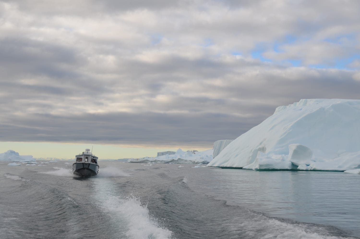
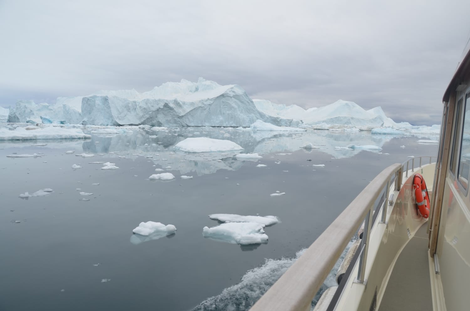
Първото прекосяване на Гренландия, или кой е Фритьоф Нансен
Post Syndicated from Светла Стоянова original https://www.toest.bg/purvoto-prekosyavanie-na-grenlandia/
<< Към цялата поредица за Гренландия

Кое е онова, което ни кара да изследваме, да дерзаем, да отиваме все по-далеч и по-далеч? Някога, но и сега. Днес почти всеки може да е полярен изследовател, но на нашите предци им е коствало много повече. Те са тръгвали към напълно непознатото без GPS и карти, защото сами са ги чертаели. Напредъкът в географските открития от онези времена е неизмеримо голям и благодарение на тях сме натрупали това знание, за да разчертаем целия свят и да го държим в ръцете си.
Но дали не сме изгубили нещо във времето?
Именно онова усещане, че отиваме на място, където не знаем какво ни очаква – непроходими планини, непознати страшни създания или пък плодородни земи, тучни и пълни със сочни плодове? Има някаква романтика в това незнание. И все пак е била нужна страхотна смелост, същинска лудост да се хукне в дивото. Много гордост е бушувала сред откривателите, защото те са ставали първите носители на новото знание. На доста от тях обаче тази амбиция е отнела и живота.
© Светла Стоянова
Като погледнем на север, кои са първите хора, които се осмеляват да търсят непознатото по онези ледовити земи? И всъщност как се развива опознаването и обуздаването на Севера през вековете?
През 330 г.пр.Хр. древногръцкият географ и астроном Питей става първият човек, който изследва най-северните ширини на планетата в търсене на кехлибар и калай. В продължение на почти хиляда години никой не тръгва по стъпките му, докато чак през Ренесанса морските държави в Европа са обхванати от треска за изследване на Арктика. Много от тях се опитват да прокарат път през Северния ледовит океан, за да търгуват по-бързо и по-лесно с Азия.
Новите екзотични стоки били твърде изкушаващи – например коприната, която правела дрехите нежни и леки за носене, и подправките, които овкусявали и най-блудкавите ястия. По онова време тези стоки пристигали по Пътя на коприната, но това било твърде продължително и скъпо. Затова благодарение на сравнително точната представа за земното кълбо някои европейски търговци решават, че преминаването на север от Европа и Америка ще съкрати значително времето за пътуване. Затова страни като Франция, Великобритания и Холандия се опитват да проправят своите маршрути все по̀ на север.
Пионерите
През 1878 г. шведът Адолф Ерик Нурденшолд прекосява за първи път Североизточния проход1. Той е искал да свърже шведските пристанища на Балтийско море с големите руски устия в северната част на континента. Почти трийсет години по-късно Северозападният проход2 също е преодолян, но от норвежеца Руал Амундсен, чийто успех се дължи на факта, че със сравнително малкия си кораб успява да маневрира през лабиринта от острови и да плава в плитки води.
Негов предшественик и сънародник е Фритьоф Нансен – полярен изследовател и ръководител на първите норвежки експедиции в Арктика. Той е учен и писател, един от пионерите в океанографията и има голям принос в картографирането на Северния ледовит океан. Две от най-значимите му експедиции са прекосяването на Гренландия и преминаването през леда на Северния ледовит океан на борда на новаторския кораб „Фрам“. Също така той допринася за спасяването на стотици хиляди хора преди и след Първата световна война, за които организира международни акции за даряване на храна на гладуващите и за връщане на военнопленници по родните им места.
Но как изобщо се става полярен изследовател?
Още двайсетгодишен, Фритьоф Нансен се включва в няколкомесечно пътуване на ловен кораб за тюлени. Тогава той за първи път стига до плаващите ледове около бреговете на Гренландия и това предопределя живота му. Там се учи да живее в открития океан и да ловува морски бозайници, което ще се окаже ценен опит за собствените му експедиции. Споменът за огромните ледени маси, носещи се в океана, и тяхното тихо величие ще продължава да го тегли нататък.
Един ден младият Фритьоф научава от вестникарска статия за опита на шведския професор Нурденшолд за прекосяване на Гренландия и нейния ледник, втория най-голям на земята след Антарктида. Стратегията на професора била да тръгне от заселения западен бряг към източния, а после да се върне по същия път, тъй като достигането на спасителен кораб от Европа до източния бряг е било невъзможно заради непроходимите късове лед в океана. Този план означавал също така, че винаги ще има спасителен път обратно, в случай че експедицията трябва да се върне поради беда или недостиг на запаси. Имало хипотези, че във вътрешността на острова съществуват оазиси с умерен климат и гори. Експедицията на Нурденшолд не постига целта си и се връща. Когато Нансен научава за това, у него пламва идеята да прекоси цяла Гренландия на ски, за да разкрие тайните на този слабо познат за човечеството остров.
Три години по-късно 26-годишният Фритьоф Нансен става ръководител на първата норвежка арктическа експедиция по прекосяване и изследване на Гренландия. Тактиката му е противоположна на всички останали подобни експедиции по негово време. Нансен решава да тръгне от изток на запад, тоест първо да стигне до слабо заселения източен бряг с малки лодки, спуснати от по-голям кораб, след което да прекоси ледника, докато накрая стигне до по-облагородения западен бряг, откъдето да се качи на кораб за Европа. Множество опитни полярници го съветват да не го прави, защото всеки добър ръководител трябва да има план за отстъпление, но младият Нансен удържа на натиска. Според него самият факт, че спасението е отпред, действа много по-мотивиращо, отколкото ако е зад гърба на тези, които с всяка крачка все повече се отдалечават от него. Затова мотото на експедицията е: „Западният бряг или смърт!“
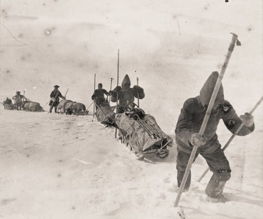
Експедицията на Нансен
На 3 юни 1888 г. Фритьоф Нансен се качва заедно с екип от още петима души на ловния кораб „Язон“. След едномесечно пътуване групата е спусната с две лодки сред плаващите ледове по източното крайбрежие на Гренландия. Оттам гребат неуморно дни наред, за да достигнат брега, и нощуват върху късове плаващ лед. След усилена борба с теченията успяват да стъпят на твърда земя. Оттам шестимата тръгват по ледника, теглейки стокилограмови шейни покрай километрични цепнатини в леда. Брулени от зловещи ветрове и снежни бури, те вървят по места, където човешки крак никога не е стъпвал. Ден след ден разпъват палатката, топят сняг, споделят оскъдни порции храна и на сутринта продължават напред в бялата пустош.
Месец и половина по-късно изследователите се спускат по западната част на ледника и достигнали брега, измайсторяват малка лодка с наличните материали, за да доплават до най-близкото населено място. В град Готхоб (дн. Нуук, столицата на Гренландия) са сърдечно приветствани от местните инуити и датчани, но се оказва, че последният кораб за Европа е заминал, и се налага да изчакат следващия до пролетта. Така те прекарват дългата зима в съжителство с гренландците, които ги обучават как да използват местните природни ресурси за храна, облекло и подслон.
По-малко от година след завръщането си на норвежка земя Фритьоф Нансен издава пътеписа Pаа ski over Grønland („На ски през Гренландия“)3, в който описва подробно експедицията, основавайки се на своя дневник и богатите си научни изследвания по пътя. Освен пътеписа той издава и книгата Eskimoliv („Животът на ескимосите“), в която подробно разказва за живота и обичаите на местното гренландско население.
Прекосяването на Гренландия и другите му експедиции в Арктика безспорно поставят началото на ново отношение на норвежците към полярните региони – от опасни и непристъпни те се превръщат в досегаеми и преодолими територии за малката норвежка нация. В резултат на дейността и творчеството си Нансен вдъхновява не само младите норвежци, но и младежите в цяла Европа за повече спорт на открито, движение сред природата и постигане на хармония между духа и тялото.
От полярник към защитник на онеправданите
Впоследствие Фритьоф Нансен засилва своята обществена дейност и става върховен комисар на Обществото на народите4. Организацията се обръща към него с молба да ръководи работата по изпращането на голям брой военнопленници в родните им страни след Първата световна война. По негова идея се въвежда официален международно признат документ – Нансенов паспорт, създаден специално за военновременните и политическите бежанци, който им позволява да пътуват безпрепятствено по света и да живеят пълноценен живот. Повече от половин милион военопленници са успешно репатрирани в родните им страни, а за работата си Нансен получава Нобелова награда за мир.
Нансенови паспорти получават и хиляди българи от Западна Тракия, депортирани от Егейските острови по време на Гръцко-турската война през 1919–1922 г., които успяват да се завърнат в родината си. Много българи днес имат прародители с Нансенов паспорт. Освен това Нансен се застъпва за България и нейното включване в ОН, а също така осигурява два заема, които помагат на държавата ни да излезе от следвоенната криза.
Фритьоф Нансен оставя дълбока следа в историята на страната си и на света. Дейността му като полярник и като хуманист има съществено значение за живота на хиляди хора. Творбите му и днес намират своя широк кръг от читатели и все така вдъхновяват малки и големи.

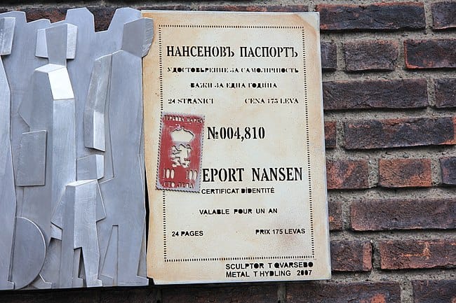
Монумент в чест на Нансеновия паспорт в кметството на Осло, Норвегия. Изложен е българският вариант на паспорта © Светла Стоянова
В днешно време продължават да се организират експедиции за прекосяването на гренландския ледник и всеки достатъчно добре подготвен физически, психически и финансово би могъл за четири-пет седмици да покори Гренландия. Но въпросът е друг.
Можем ли днес да бъдем изследователи?
Има ли още непокорени земи и неразчертани карти? Можем ли да продължим да опознаваме света наоколо със същото нестихващо любопитство и после с радост да споделяме откритията си с другите? Можем ли да запазим онази детска дързост за откривателство и да не я пускаме да отлети с годините?
1 Североизточният проход минава северно от скандинавските страни и по цялото протежение на Русия, за да стигне до Китай, вместо значително по-дългия път през Средиземно море, Червено море и целия Индийски океан, за да се стигне отново до Китай.
2 Северозападният проход минава южно от Гренландия, провира се между канадските острови, за да стигне отново до Азия.
3 Пътеписът е преведен от руски език от И. П. Кепов и публикуван на български през 1898 г. от изд. „Христо Г. Данов“ под заглавието „Гренландия. Географски очерк на страната и разказ за пътешествието на Фр. Нансен“.
Фалшът като публична психотерапия
Post Syndicated from original https://www.toest.bg/falshut-kato-publichna-psihoterapiya/

Книгата „Post-Truth“ („Постистина“) на Лий Макинтайър, изследовател в Центъра по философия и история на науката към Бостънския университет, започва с кратък откъс от разговор между журналистката от Си Ен Ен Алисън Камерота и тръмписта Нют Гингрич. В откъса Камерота казва, че САЩ е по-безопасна страна, защото националната статистика на ФБР показва намаляване на престъпността. Гингрич контрира с тезата, че това не е съвсем вярно, защото хората се чувстват по-незащитени. Върнат отново към фактите, той заявява, че ще се довери на усещанията на хората и ще остави на репортерката статистиката на либералните теоретици.
Няколко години по-късно (през 2024 г.), няколко месеца преди поредните предсрочни избори в България, в телевизионно студио един от по-известните коментатори на политическия живот и пламенен защитник на най-голямата партия в страната, след кратък обмен на реплики с водещата заявява: „Ако искаме да се вторачим във фактологията през годините, най-вероятно ще съумеем да го [лидера на най-голямата партия и три пъти премиер – б.а.] опровергаем, но не тя е важната.“
След което българската журналистика, съвсем свободно оставена в бурята на фактите и впечатленията, сменя темата и признанието, че фактологията не е „важното“, оставя проблема да изтлее във вакуума на обществения ни дискурс. Важно е посланието – това, което трябва да се разбира отвъд лъжата. А тя е просто подробност, на която няма нужда да обръщаме внимание.
Дума на всички години
Феноменът постистина придоби по-широка популярност през 2016 г., когато бе обявена за дума на годината на Оксфордските речници заради огромния скок в употребата ѝ спрямо предходната година. Това става неслучайно във вихъра на две кампании – след едната Доналд Тръмп бе избран за президент на САЩ, а след другата във Великобритания се стигна до Брекзит. В месеците на информационни битки и злоупотреби емоциите сякаш бяха избутали фактите в ъгъла и дезинформацията изпревари проверената информация в съзнанието на хората в две от най-големите демокрации в света.
Дали самият термин е станал моден за ограничен период, или предстои да се закотви в специализирания публичен дискурс, включително в академичния, е отделна тема, но промените в начина, по който употребяваме и създаваме информация, и ефектите от тези промени са съвсем реални.
Какви са обаче причините все по-често да се обръщаме към усещанията си, а не към фактите, за да търсим истината?
Надали някой би се наел със задачата да ги посочи изчерпателно, но има някои ясни обществени феномени, които водят до фалшивия избор между обоснованите мнения на едни и личните впечатления на други. Един такъв феномен е базисното недоверие на вторите спрямо първите. В България то се наблюдава директно, но обществото ни изобщо не е изолирано от света, що се отнася до презумпцията за измама, която свободно прилага към определени професионални кръгове.
Ние не вярваме на експертите, защото повтарят опорките на господарите си и са платени от чужди агенти. Не вярваме на интелектуалците, защото не са свършили работа за пет стотинки и единственото, което правят, е да приказват празни приказки. Не вярваме на лекарите, защото искат да ни пробутат дадено лекарство, за което получават пари. Някои искат и да ни чипират. Тези са най-зли, защото ненавиждат народа си и помагат на по-висши сили да го унищожат.
Ниското доверие към експертността е повсеместно там, където има реална демокрация. На другите места няма значение – там истината има един първоизточник и второ мнение не съществува, поне не задълго. Развитието на по-свободните общества обаче е напреднало до такава степен, че разстоянията между социалните групи стават наистина големи. Измерването на неравенствата показва донякъде тези разстояния, но като се има предвид, че първото, за което мислим в контекста на неравенства, е материалното, то публичното е плоскостта, която разкрива различията много по-нюансирано. Именно там бива изразено това недоверие – в практиките на информиране, в израза на нагласите на различните групи, в гласуването.
Пазарът на мнения в публичността
Си Ен Ен е първата телевизия, залагаща на бизнес модел, който изцяло се занимава с излъчване на новини. Създадена е през 1980 г. и за три години излиза на печалба – нещо немислимо за американския медиен пазар, където дотогава новините са въпрос на престиж и/или необходимост, а не източник на приходи. А събитията, подхранващи нуждата от непрестанно информиране, изобилстват. Новината сама по себе си обаче не отговаря на въпроса какво се случва. Нито казва експлицитно кой е прав и кой – не. Новината е нещо неутрално, подлежащо на интерпретация.
Преди появата на „Фокс Нюз“ на сцената излиза радиоводещият Ръш Лимбо, който въвежда прийом, използван в много предавания и до днес – директно включване на зрители в ефир. Предаването му става национално през 1988 г., форматът е коментарен, а възгледите му са консервативни. Така възприеманите за демократични медии намират своята конкуренция в токшоу, което има за цел не да излъчва новини, а да ги обсъжда. И това с прякото участие на Негово Величество Зрителя, който е поставен на недостижимия дотогава пиедестал на владетел на истината.
През 1996 г. е основана и телевизия „Фокс Нюз“ – най-мощният мегафон на американския консерватизъм. Но истинският проблем е в това, че изследване от 2006 г. показва как 68% от историите във „Фокс Нюз“ отразяват лични мнения, докато в Си Ен Ен такива са едва 4%.
Пазарът решава. Пазарът на мнения в публичността. Недоверието на една голяма част от американците към другите е удовлетворено. Слушателите на Лимбо са филтрирани, гостите във „Фокс“ – също. Партизанщината в медиите се ожесточава, а чистата информация вече няма как да бъде интересна, защото каква е стойността ѝ, ако не бъде положена в контекст и обяснена? Но обяснена не така, че да носи реално разбиране на обществените процеси, а така, че да носи удовлетворение. Да бъде отдушник за психическото напрежение, което усложняващият се свят носи. Да насочи погледа в конкретна посока, да го канализира, защото скоростта, с която се случват нещата наоколо, се увеличава скокообразно, а в това ускоряване (заемам термина от Хартмут Роза) неизбежно някои изостават и/или се объркват.
Намирането на враг като опит за справяне с тревожността
И тук стигаме до един друг феномен, който оказва влияние върху това как създаваме и консумираме информация. Тревожността е страх, който няма обект. Тя е чувство за напрежение без ясен източник. Просто е там, постоянството ѝ създава с времето ефект, който става все по-труден за вътрешно обработване, и ние трябва спешно да намерим решение, защото ще се взривим. Сякаш най-ефикасно се оказва намирането на враг – източник на напрежението, на страха, на несигурността. Колкото по-добре оформен е врагът, толкова повече спада тревожността. Поне на пръв поглед, докато не се появи нещо ново, което ще трябва да разгледаме под лупа, за да подредим в съзнанието си.
Но ако обърнем внимание на ефектите от посочването на виновника, ще можем да си обясним, поне в някаква степен, защо съвременните демократични общества, включително българското, формират определени антидемократични нагласи, а някои дори си избират и лидери, които са чиста форма автократи.
Пропагандата, заливаща българското медийно пространство, злоупотребява именно с такива настроения. Тръгвайки от непосредствените страхове от въвличане във войната между Русия и Украйна, можем да се върнем назад, за да установим, че преди това се страхувахме от COVID-19, преди това – от нестабилността покрай протестите, преди това – от членството в НАТО и ЕС, и т.н.
Страхът и яростта често са ефект от неразбирането, което се дължи не на глупост, а на един объркан инстинкт, който еволюционно ни е посочвал потенциалната опасност в непосредствената ни среда, за да ни пази. А сега, когато трябва да се справим с обяснението на все повече и все по-сложни обществени процеси, търсим истината на места, които ни дават всички уверения, че ще удовлетворят терзанията ни.
Страхуваме се от мигрантите, защото не сме виждали такива, но въпреки това предизвикват ярост у нас. Страх ни е от война, защото определена част от елита ни са „войнолюбци“ и им се гневим. Страх ни е за традиционното семейство, защото все по-малко двойки сключват брак, но не си даваме сметка за социално-икономическите фактори за това, а сме насъскани да мразим либерализма и т.нар. джендъри (каквото и да значи това) като плашилото, бутащо българското общество към бездната на демографската катастрофа. В същото време чувстваме, че не просперираме икономически, но наблюдаваме увеличаващото се благосъстояние на определени групи хора. И смятаме това за несправедливо, понякога с пълно право, доколкото е реален факт престъпното акумулиране на богатства в определени кръгове (най-успешни са онези измами, в които има доза истина).
Но на масата, както изисква Негово Величество Зрителят, имаме всички възможни решения. Тези от левия политически спектър искат да вземат от богатите, за да дадат на бедните. Отдясно се говори за национално капсулиране с цел запазване на култура, бит и автентичност. Трети прикриват запазването на престъпната си власт под фалшивия прагматизъм на една измамна стабилност. Но във всички случаи се изправяме пред враг, който ни мисли злото, и нашият инстинкт е да се фокусираме върху него.
Подмяната на реалността
В такава ситуация най-големият герой за нас би бил този, който ни посочва врага. Понякога това се случва отвън – популизмът или някой по-обигран коментатор прави точно това. Понякога идва отвътре – убеждението, че сами сме стигнали до ядрото на проблема. Понякога демагогията (например война или нестабилност) ни разказва една проста, ясна и логична теория, която ни помага да разберем кой и как точно ни мисли злото. Комплексността на социалните процеси е минимизирана, а фаровете ни сочат тънката червена линия към острова на изгубеното съкровище.
В демократичните общества проблемите все по-трудно остават скрити. И това е добре, но засилването на тревожността предпоставя наличието на постоянен стремеж към търсене и елиминиране на причините за тези проблеми. И макар това да е едно наистина благородно начинание, усложняването на обществените взаимоотношения и процеси го прави все по-трудоемко и ролята на експертите става все по-важна.
С проблемите обаче се усложняват и решенията. Поне докато не се появи някой, който да даде простите обяснения, а с тях – и надежда. Месията обръща очи, потвърждава вече наличното знание, нарежда нещата, които не са ни ясни, носи комфорт, отпуска и мотивира.
Подмяната на реалността се е превърнала в истинска психотерапия за нервния, постоянно бързащ модерен човек. Дали чрез полагането в нов контекст на неща, които сме усещали с кожата си, например при конспиративната теория, или чрез продължаващото потъване в заешката дупка на идеологическия разказ, капанът на тектоничното пренареждане на фактологията става все по-здрав, колкото по-силно искаме да повярваме.
Една обикновена фалшива новина може да бъде опровергана относително лесно, но какво усилие трябва да бъде положено, за да бъде опровергана цяла една подменена реалност, която ни обяснява света, мястото ни в него и ни дава комфорт?
В една от сцените във филма „Телевизионна мрежа“ (1976 г.) бивш водещ на новините в голяма американска телевизия изпада в делюзия и разярен от натрупаното психическо напрежение заради влошаващата се обществена обстановка, призовава зрителите да излязат на прозорците си и да започнат да крещят: I am mad as hell, and I’m not gonna take it anymore! („Бесен съм и повече няма да търпя!“). Освобождаването на напрежението има непосредствен позитивен ефект, но ако не бъде последвано от бързи и съществени промени, които да засилят усещането за справедливост, то остава просто кратък епизод на ентусиазъм.
Бързи промени в обществото ни не се виждат. Пишейки този текст в деня след поредните предсрочни избори, не мисля, че имаме шанс за нещо такова през следващите месеци, дори години. Сред все по-големи групи от българи обаче ясно се вижда фрустрацията от случващото се у нас и по света. Някои търсят червената линия към пристана на стабилност, други подкрепят агентите на хаоса, които обещават бързи и радикални промени. Трети стоят разочаровани от средата, която не намира смелостта да се погледне в огледалото просто защото не смята, че има нужда. Всички са тревожни и малцина смятат, че това се дължи на нещо, което не им е вече посочено. А ако е посочено, то само яростта им ще го изплаши.
Вероятно скоро няма да видим масово висящи по балконите българи, които крещят, че са побеснели и повече няма да търпят. Но и малцината, които вероятно биха го направили, ще получат мълчаливата подкрепа на останалите. И ако новинарят от „Телевизионна мрежа“ е изпаднал в състояние на амок и продуцентите на телевизията му създават специално шоу, в което той да изкрещява всичко онова, което си мисли публиката, то за нас е от огромна необходимост да удържим методите си за справяне с напрежението и с реалните проблеми в лоното на фактите и истината, защото при всяко положение попадаме в теоремата на Томас. А според нея интерпретацията на дадена ситуация е в основата на последващото наше действие. Тоест една нереална ситуация може да има съвсем реални последствия, ако сме твърдо убедени, че тя е именно такава.
Comic for 2024.06.14 – All Of My Haters
Post Syndicated from Explosm.net original https://explosm.net/comics/all-of-my-haters
New Cyanide and Happiness Comic
Capturing a Tiger
Post Syndicated from The History Guy: History Deserves to Be Remembered original https://www.youtube.com/watch?v=Z7Kh_LnYFew
1.2 Kilofives
Post Syndicated from xkcd.com original https://xkcd.com/2946/

ASUS ROG NUC Review Really Good With Intel and NVIDIA RTX 4070
Post Syndicated from Patrick Kennedy original https://www.servethehome.com/asus-rog-nuc-review-really-good-with-intel-and-nvidia-rtx-4070/
In our ASUS ROG NUC review, we see how expanding the NUC to 2.5L allows a high-end Intel Core Ultra 9 and NVIDIA GeForce RTX 4070 to fit
The post ASUS ROG NUC Review Really Good With Intel and NVIDIA RTX 4070 appeared first on ServeTheHome.