This is a guest post by Kinsta about their use of our platform.
At Kinsta, we’re obsessed with speed: Our Application Hosting, Database Hosting and Managed WordPress Hosting services all run on the Google Cloud Platform’s fastest Premium Tier Network and C2 Machines, and we rely on Cloudflare to keep the pedal to the metal for tens of thousands of customers who want to deliver their content around the world with speed and security.
While making that happen, we’ve learned a thing or two about using Cloudflare Workers and Workers KV to provide optimized caching rules for static and dynamic content.
In early 2023, we doubled down on Cloudflare cache wrangling, making caches more responsive to client-side configuration changes while also shifting the heavy lifting behind broadcasting feature updates away from our admins on the backend and into Cloudflare Workers. A key result was a dramatic increase in the share of customer data successfully cached, increasing 56.3% between October 2022 and March 2023.
Cloudflare Workers and Workers KV allow us to programmatically customize every request and response with minimal effort and lower latency. We no longer need to deploy changes to hundreds of thousands of containers when we want to implement new features; we can replicate or implement the feature with Workers and deploy it everywhere with a few commands and clicks, saving us days of work and maintenance.
Request routing with Workers KV and Workers
Every Kinsta-hosted domain is a key, and its value contains at least the core settings, like the origin's IP and port, and a unique random ID. With this data easily available in Workers KV, we can use Workers to analyze, manipulate, and route requests to their expected backend. We also use Workers KV to store customer optimization options like Polish, Image Resizing, and Auto Minify.
To route requests to custom IPs and ports, we use resolveOverride, a Cloudflare-specific Request property. Here's an example:
However, while Workers KV worked well to route requests, we soon noticed inconsistent responses in our cache. Sometimes a customer activated Polish and, due to Workers KV's one-minute cache, new requests arrived before Workers KV fully propagated the change, causing us to cache non-optimized assets. When this happened, the client had to clear their cache again manually. Not the ideal scenario. Clients got frustrated, and we wasted API operations and GCP bandwidth, constantly purging caches.
Cache key is the key
Since we always read the domain's Workers KV data, we realized we could route requests and customize the cache key, appending things like the domain's ID and features that could affect the asset, like Polish. Today, our cache key is heavily customized to quickly reflect every client's change in our panel or API. By modifying the cache key using Workers KV's data, nobody needs to worry about clearing the cache anymore. As soon as Workers KV propagates the changes, the cache key also changes and we request and cache a fresh asset.
The easiest way to customize the cache key is to append query params to it. For example:
<pre><code class="language-javascript">
let cacheKey = `${request.url}?custom-cache-param-polish=lossy`
</code></pre>
Of course, you need to check the URL for existing parameters to determine which connector to use — ? or & — and ensure you are using a unique identifier.
Then, you can use this new cache key to save the response with Cache API or Fetch — or both.
Workers KV Cache
Workers KV operations are affordable, but the numbers can pile up when you trigger billions of reading operations daily.
Thanks to our cache key customization, we realized we could cache the Workers KV data with Cache API, saving on reading operations and possibly lowering the latency by avoiding multiple Workers KV GET requests per visitor. Since the cached response is now based on the request's URL combined with KV data, we no longer need to worry about caching stale content.
However, unlike many applications, we can't cache Workers KV for extended periods. Kinsta's customers are constantly trying new features, changing Polish and Auto Minify settings, sometimes excluding pages or extensions from being cached, and they want to see their changes in production as soon as possible.
That's when we decided to microcache our Workers KV data — caching dynamic or constantly-changed content for a very short period of time, usually less than 60 seconds.
It’s pretty simple to implement your own Workers KV caching logic. For example:
<pre><code class="language-javascript">
const handleKVCache = async (event, myCustomDomain) => {
  // Try to get KV from cache first
  const cache = caches.default;
  let site_data = await cache.match( `https://${myCustomDomain}/some-string-ID-kv-data/` );

  // Valid KV cache match
  if (site_data && site_data.status === 200) {
    // ... modify your cached data if necessary, then return it
    return site_data;
  }

  // Invalid cache (expired, miss, etc), get data from KV namespace
  site_data = await KV_NAMESPACE.get(myCustomDomain.toLowerCase());

  // Cache valid KV responses with Cache API
  if (site_data) {
    let kvResponse = new Response(JSON.stringify(site_data), {status: 200});
    kvResponse.headers.set("Cache-Control", "public, s-maxage=30");
    event.waitUntil(cache.put(`https://${myCustomDomain}/some-string-ID-kv-data/`, kvResponse));
  }

  return site_data;
};
</code></pre>
This article was written by Ethan Smart, Co-Founder and Chief Solution Architect, appNovi (a Rapid7 integration partner).
It’s essential for security and IT teams to have a comprehensive view and control of their cyber assets. This is why Cyber Asset Attack Surface Management (CAASM) has received so much attention from security practitioners and leaders.
According to Gartner, “CAASM tools use API integrations to connect with existing data sources of the organization. These tools then continuously monitor and analyze detected vulnerabilities to drill down the most critical threats to the business and prioritize necessary remediation and mitigation actions for improved cyber security.”
CAASM provides a unified view of all cyber assets to identify exposed assets and potential security gaps through data integration, conversion, and analytics. It is intended to be authoritative source of asset information complete with ownership, network, and business context for IT and security teams.
Security teams integrate CAASM with existing workflows to automate security control gap analysis, prioritization, and remediation processes. These integration outcomes boost efficiency and break down operational silos between teams and their tools. Common key performance indicators of CAASM are asset visibility, endpoint agent coverage, SLAs, and MTTR.
It’s important to understand assets are more than devices and infrastructure. In a Security Operations Center (SOC), assets include users, applications, and application code. Recognizing the interconnectedness of these assets is key to enhancing the SOC’s capabilities. For example, consider a scenario where 1,000 servers have the same vulnerability. Assessing each one individually would be incredibly time-consuming. CAASM enriches cyber asset data to automate the majority of analysis.
For example, when you understand only eight of the 1,000 servers are internet-facing, and of those only two are exposed through the necessary port and protocol for exploitation of the vulnerability, you know which assets have the highest contextual exposure, which are exploitable, and which should be addressed first.
In this blog, we’ll cover how security teams can leverage their existing tech stack for Cyber Asset Attack Surface Management.
Understanding the Attack Surface
Comprehensive attack surface management hinges on a comprehensive understanding of everything that is a target for attackers. In a sprawling enterprise environment, there’s an abundance of assets distributed across different networks (e.g. cloud, SDN, on-prem), each with its own set of monitoring and alerting tools. When these security tools don’t interoperate or mesh with one another, security teams lack a complete picture of the attack surface. This fragmented understanding results in the continued siloing of teams and tools and inhibits effective data sharing.
One of the oldest adages in cybersecurity is complexity is the enemy of security—and complexity increases when teams recognize assets as more than devices. Assets are more than just computers and servers connecting on the network, as those assets are used to support applications to drive revenue. Applications also use code, which can be used by multiple applications. Users are assets that operate the business using technology. This complex asset tracking and relationship mapping spans network connections, application and code ownership, and the dependencies and indirect dependencies between applications.
CAASM emerged to address this complexity. CAASM is founded through the consolidation of existing data from all the different network and security tools. For example, by integrating Rapid7’s portfolio of products with a security data integration and visualization solution like appNovi, organizations can achieve and maintain full visibility across their entire connected network—including on-prem, Software Defined Network (SDN), and hybrid cloud.
Using CAASM, organizations can leverage analytics to refine search results, identify trends, or disseminate specific information to defined groups or individuals. One common use case with appNovi is identifying vulnerable application servers contextually exposed for exploitation and identifying owners based on login telemetry and notifying the server owner and security. This integrated approach delivers comprehensive attack surface visibility and mapping to enable organizations to address risks and manage vulnerabilities more efficiently. When analytics are coupled with automation tools, such as orchestrators, the SOC is able to focus on threat hunting and less on data analysis. Common examples include asset inventory management and security control gap analysis.
Cyber Asset Inventory and Mapping
To manage the attack surface proficiently, it’s essential to discover and map an organization’s assets accurately and with the greatest level of detail. Organizations that use Rapid7’s Insight Platform already identify network infrastructure to pinpoint active devices, open ports, and running services. When combined with your other tools’ data through the enrichment capabilities of appNovi, Rapid7’s InsightVM integrates with the entire network and security tech stack to reveal overlooked assets, those that were inadvertently deployed without endpoint detection and response (EDR) agents, and those that require a prioritized response.
Telemetry data can also be leveraged from Rapid7’s InsightIDR to enrich asset data to understand network connections, ownership, and user activity. This relationship and connection mapping supports establishing the relationships between assets and their relevance to applications. With an automated and continuously updated asset inventory enriched by telemetry, IT and security teams not only gain visibility but also develop a comprehensive understanding of each asset’s dependencies and business significance.
Risk Assessment and Prioritization Based on Exposure
Vulnerability scanners and agents help you understand what devices and their software are vulnerable. For teams today to understand the exposure of their vulnerable devices requires sifting through large amounts of network log data. This time-consuming process often inhibits the ability to prioritize devices based on their network contextual exposure. But when telemetry sources are abstracted and converged with cyber asset data, contextual exposure analysis becomes a simple and automated analysis. That’s why data convergence in appNovi with Rapid7’s platform compiles network, asset, and vulnerability data into a comprehensive and easily accessible format.
This powerful data management capability means teams efficiently and accurately identify the devices that are the most vulnerable and exposed to both external threats and lateral movement from within the network. With this level of enrichment, security teams can quickly identify the handful of assets that require immediate prioritization to support an effective remediation strategy.
Identifying and Managing New Assets
Monitoring the attack surface involves leveraging a diverse set of tools to identify new assets within an organization’s digital ecosystem. It is vital to utilize comprehensive asset discovery tools, vulnerability scanners, and other solutions to gain a holistic view of the digital infrastructure.
However, some infrastructure is ephemeral or may be inaccessible to all monitoring tools, in which case telemetry data sources and other SIEM data can be used to identify new assets. This aggregation, enrichment, and analysis can feed into other actions whether it be as simple as email notifications of results or triggering specific automated actions.
Creating Closed-Loop Remediation
When an authoritative source of detailed asset data is established standard searches can be run to provide consistent results and define specific outcomes. As an example, many organizations want to prioritize appropriate EDR agent and Rapid7 IDR agent installations across their application infrastructure.
To achieve this functionality, security teams define what constitutes appropriate security controls and search for all assets that do not meet the criteria. The results can trigger playbooks or workflows to create automated remediation notifications. In instances where orchestrators can install agents, those assets without agents can be automatically remediated in a self-healing loop.
By integrating Rapid7’s platform with appNovi, businesses gain actionable insights into the changes that occur across their attack surface with the ability to implement streamlined remediation.
Best Practices for Cyber Asset Attack Surface Management
Maintaining a robust attack surface management initiative is essential—automating as much of it as possible is what will result in efficiencies for the SOC. There are several best practices for organizations that want to undertake the initiative to uplevel security operations with Cyber Asset Attack Surface Management.
Different data, same problem Rarely is all data in the same format. Even more rarely does all data provide the same match values of assets. For CAASM to be effective, ingestion and data convergence must facilitate data normalization through abstraction. This needs to be done through unique identifiers. Without integrated data feeds that support the wide variety of data structures and vendor nuances, you’ll end up back in an Excel spreadsheet that effectively only saves you a SIEM query.
Less is hard There are many different data points about assets. All the asset attributes must converge into a single asset profile. Without this capability, security teams will be sifting through duplicate records providing two different perspectives on the same asset which often leads to partial resolution or inaction. To be effective, the SOC needs a high-fidelity source of data and not several incomplete profiles of the same asset.
Where is it? Complete asset inventories are helpful to satiate compliance requirements, but without context, all assets will be viewed based on an objective data point. Because you have network data, you should be able to apply your network context to it and make the asset subjective. An external-facing asset with a medium risk is more important than a high risk asset buried behind several network security controls. Your tools already monitor and have network and business context—that telemetry and enrichment need to extend to assets.
What is it? Every enterprise has applications. Few know how many they have deployed in their network. Using application data sources can help delineate and track application servers and what they are direct and indirect dependencies of. The business importance of an asset helps not only in prioritization, but telemetry such as logins can expedite ownership identification.
Conclusion
By leveraging the power of CAASM, organizations can overcome the complexity of asset tracking and relationship mapping, optimize their security workflows, and effectively manage the evolving threat landscape. The tooling already exists, all that’s required is the integration and data convergence capabilities for you to uplevel the SOC.
Watch appNovi’s video on CAASM capabilities with Rapid7 today to understand this comprehensive and proactive approach to cybersecurity.
Security updates have been issued by Debian (libfastjson, libx11, opensc, python-mechanize, and wordpress), SUSE (salt and terraform-provider-helm), and Ubuntu (firefox, libx11, pngcheck, python-werkzeug, ruby3.1, and vlc).
Zabbix is highly regarded for its ability to integrate with a variety of systems right out of the box. That list of systems has recently been expanded with the addition of Event-Driven Ansible. Bringing Zabbix and Event-Driven Ansible together lets you completely automate your IT processes, with Zabbix being the source of events and Ansible serving as the executor. This article will explore in detail how to send events from Zabbix to Event-Driven Ansible.
What is Event-Driven Ansible?
Currently available in developer preview, Event-Driven Ansible is an event-based automation solution that automatically matches each new event to the conditions you specified. This eliminates routine tasks and lets you spend your time on more important issues. And because it’s a fully automated system, it doesn’t get sick, take lunch breaks, or go on vacation – by working around the clock, it can speed up important IT processes.
Sending an event from Zabbix to Event-Driven Ansible
From the Zabbix side, the implementation is a media type that uses a webhook – a tool that’s already familiar to most users. This solution allows you to take advantage of the flexibility of setting up alerts from Zabbix using actions. This media type is delivered to Zabbix out of the box, and if your installation doesn’t have it, you can import it yourself from our integrations page.
On the Event-Driven Ansible side, the webhook plugin from the ansible.eda standard collection is used. If your system doesn’t have this collection, you can get it by running the following command:
ansible-galaxy collection install ansible.eda
Let’s look at the process of sending events in more detail with the diagram below.
From the Zabbix side:
An event is created in Zabbix.
The Zabbix server checks the created event according to the conditions in the actions. If all the conditions in an action configured to send an event to Event-Driven Ansible are met, the next step (running the operations configured in the action) is executed.
Sending through the “Event-Driven Ansible” media type is configured as an operation. The address specified by the service user for the “Event-Driven Ansible” media is taken as the destination.
The media type script processes all the information about the event, generates a JSON, and sends it to Event-Driven Ansible.
From the Ansible side:
An event sent from Zabbix arrives at the specified address and port. The webhook plugin listens on this port.
After receiving an event, ansible-rulebook starts checking the conditions in order to find a match between the received event and the set of rules in ansible-rulebook.
If the conditions for any of the rules match the incoming event, then the ansible-rulebook performs the specified action. It can be either a single command or a playbook launch.
Let’s look at the setup process from each side.
Sending events from Zabbix
Setting up sending alerts is described in detail on the Zabbix – Ansible integration page. Here are the basic steps:
Import the media type of the required version if it is not present in your system.
Create a service user. Select “Event-Driven Ansible” as the media and specify the address of your server and the port which the webhook plugin will listen in on as the destination in the format xxx.xxx.xxx.xxx:port. This article will use the value 5001 as the port. This value will still be needed to configure ansible-rulebook.
Configure an action to send notifications. As an operation, specify sending via “Event-Drive Ansible.” Specify the service user created in the previous step as the recipient.
Receiving events in Event-Driven Ansible
First things first – you need to have an eda-server installed. You can find detailed installation and configuration instructions here.
After installing an eda-server, you can make your first ansible-rulebook. To do this, you need to create a file with the “yml” extension. Call it zabbix-test.yml and put the following code in it:
---- name: Zabbix test rulebook hosts: all sources: - ansible.eda.webhook: host: 0.0.0.0 port: 5001 rules: - name: debug condition: event.payload is defined action: debug:
Ansible-rulebook, as you may have noticed, uses the yaml format. In this case, it has 4 parameters – name, hosts, source, and rules.
Name and Host parameters
The first 2 parameters are typical for Ansible users. The name parameter contains the name of the ansible-rulebook. The hosts parameter specifies which hosts the ansible-rulebook applies to. Hosts are usually listed in the inventory file. You can learn more about the inventory file in the ansible documentation. The most interesting options are source and rules, so let’s take a closer look at them.
Source parameter
The source parameter specifies the origin of events for the ansible-rulebook. In this case, the ansible.eda.webhook plugin is specified as the event source. This means that after the start of the ansible-rulebook, the webhook plugin starts listening in on the port to receive the event. This also means that it needs 2 parameters to work:
Parameter “host” – a value of 0.0.0.0 used to receive events from all addresses.
Parameter “port” – with 5001 as the value. This plugin will accept all incoming messages received on this particular port. The value of the port parameter must match the port you specified when creating the service user in Zabbix.
Rules parameter
The rules parameter contains a set of rules with conditions for matching with an incoming event. If the condition matches the received event, then the action specified in the actions section will be performed. Since this ansible-rulebook is only for reference, it is enough to specify only one rule. For simplicity, you can use event.payload is defined as a condition. This simple condition means that the rule will check for the presence of the “event.payload” field in the incoming event. When you specify debug in the action, ansible-rulebook will show you the full text of the received event. With debug you can also understand which fields will be passed in the event and set the conditions you need.
The name, host, source parameters only affect the event source. In our case, the webhook plugin will always be the event source. Accordingly, these parameters will not change and in all the following examples they will be skipped. As an example, only the value of the rules parameter will be specified.
To start your ansible-rulebook you can use the command:
The line Waiting for events in the output indicates that the ansible-rulebook has successfully loaded and is ready to receive events.
Examples
Ansible-rulebook provides a wide variety of opportunities for handling incoming events. We will look into some of the possible conditions and scenarios for using ansible-rulebook, but please remember that a more detailed list of all supported conditions and examples can be found on the official documentation page. For a general understanding of the principles of working with ansible-rulebook, please read the documentation.
Let’s see how to build conditions for precise event filtering in more detail with a few examples.
Example #1
You need to run a playbook to change the NGINX configuration at the Berlin office when you receive an event from Zabbix. The host is in three groups:
Linux servers
Web servers
Berlin.
And it has 3 tags:
target: nginx
class: software
component: configuration.
You can see all these parameters in the diagram below:
On the left side you can see a host with configured monitoring. To determine whether an event belongs to a given rule, you will work with two fields – host groups and tags. These parameters will be used to determine whether the event belongs to the required server and configuration. According to the diagram, all event data is sent to the media type script to generate and send JSON. On the Ansible side, the webhook receives an event with JSON from Zabbix and passes it to the ansible-rulebook to check the conditions. If the event matches all the conditions, the ansible-rulebook starts the specified action. In this case, it’s the start of the playbook.
In accordance with the specified settings for host groups and tags, the event will contain information as in the block below. However, only two fields from the output are needed – “host_groups” and “event_tags.”
First, you need to determine that the host is a web server. You can understand this by the presence of the “Web servers” group in the host in the diagram above. The second point that you can determine according to the scheme is that the host also has the group “Berlin” and therefore refers to the office in Berlin. To filter the event on the Event-Driven Ansible side, you need to build a condition by checking for the presence of two host groups in the received event – “Web servers” and “Berlin.” The “host_groups” field in the resulting JSON is a list, which means that you can use the is select construct to find an element in the list.
Search by tag value
The third condition for the search applies if this event belongs to a configuration. You can understand this by the fact that the event has a “component” tag with a value of “configuration.” However, the event_tags field in the resulting JSON is worth looking at in more detail. It is a dictionary containing tag names as keys, and because of that, you can refer to each tag separately on the Ansible side. What’s more, each tag will always contain a list of tag values, as tag names can be duplicated with different values. To search by the value of a tag, you can refer to a specific tag and use the is select construction for locating an element in the list.
To solve this example, specify the following rules block in ansible-rulebook:
  rules:
    - name: Run playbook for office in Berlin
      condition: >-
        event.payload.host_groups is select("==","Web servers") and
        event.payload.host_groups is select("==","Berlin") and
        event.payload.event_tags.component is select("==","configuration")
      action:
        run_playbook:
          name: deploy-nginx-berlin.yaml
Solution
The condition field contains 3 elements, and you can see all conditions on the right side of the diagram. In all three cases, you can use the is select construct and check if the required element is in the list.
The first two conditions check for the presence of the required host groups in the list of groups in “event.payload.host_groups.” In the diagram, you can see with a green dotted line how the first two conditions correspond to groups on the host in Zabbix. According to the condition of the example, this host must belong to both required groups, meaning that you need to set the logical operation and between the two conditions.
In the last condition, the event_tags field is a dictionary. Therefore, you can refer to the tag by specifying its name in the “event.payload.event_tags.component“ path and check for the presence of “configuration” among the tag values. In the diagram, you can see the relationship between the last condition and the tags on the host with a dotted line.
Since all three conditions must match according to the condition of the example, you once again need to put the logical operation and between them.
Action block
Let’s analyze the action block. If both conditions match, the ansible-rulebook will perform the specified action. In this case, that means the launch of the playbook using the run_playbook construct. Next, the name block contains the name of the playbook to run: deploy-nginx-berlin.yaml.
Example #2
Here is an example using the standard template Docker by Zabbix agent 2. For events triggered by “Container {#NAME}: Container has been stopped with error code”, the administrator additionally configured an action to send it to Event-Driven Ansible as well. Let’s assume that in the case of stopping the container “internal_portal” with the status “137”, its restart requires preparation, with the logic of that preparation specified in the playbook.
There are more details in the diagram above. On the left side, you can see a host with configured monitoring. The event from the example will have many parameters, but you will work with two – operational data and all tags of this event. According to the general concept, all this data will go into the media type script, which will generate JSON for sending to Event-Driven Ansible. On the Ansible side, the ansible-rulebook checks the received event for compliance with the specified conditions. If the event matches all the conditions, the ansible-rulebook starts the specified action, in this case, the start of the playbook.
In the block below you can see part of the JSON to send to Event-Driven Ansible. To solve the task, you need to be concerned only with two fields from the entire output: “event_tags” and “operation_data”:
The first step is to determine that the event belongs to the required container. Its name is displayed in the “container” tag, so you need to add a condition to search for the name of the container “/internal_portal” in the tag. However, as discussed in the previous example, the event_tags field in the resulting JSON is a dictionary containing tag names as keys. By referring to the key to a specific tag, you can get a list of its values. Since tags can be repeated with different values, you can get all the values of this tag by key in the received JSON, and this field will always be a list. Therefore, to search by value, you can always refer to a specific tag and use the is select construction.
Search by operational data field
The second step is to check the exit code. According to the trigger settings, this information is displayed in the operational data and passed to Event-Driven Ansible in the “operation_data” field. This field is a string, and you need to check with a regular expression if this field contains the value “Exit code: 137.” On the ansible-rulebook side, the is regex construct will be used to search for a regular expression.
To solve this example, specify the following rules block in ansible-rulebook:
  rules:
    - name: Run playbook for container "internal_portal"
      condition: >-
        event.payload.event_tags.container is select("==","/internal_portal") and
        event.payload.operation_data is regex("Exit code.*137")
      action:
        run_playbook:
          name: restart_internal_portal.yaml
Solution
In the first condition, the event_tags field is a dictionary and you are referring to a specific tag, so the final path will contain the tag name, including “event.payload.event_tags.container.” Next, using the is select construct, the list of tag values is checked. This allows you to check that the required “internal_portal” container is present as the value of the tag. If you refer to the diagram, you can see the green dotted line relationship between the condition in the ansible-rulebook and the tags in the event from the Zabbix side.
In the second condition, access the event.payload.operation_data field using the is regex construct and the regular expression “Exit code.*137.” This way you check for the presence of the status “137” as a value. You can also see he link between the green dotted line of the condition on the ansible-rulebook side and the operational data of the event in Zabbix in the diagram.
Since both conditions must match, you can specify the and logical operation between the conditions.
Action block
Taking a look at the action block, if both conditions match, the ansible-rulebook will perform the specified action. In this case, it’s the launch of the playbook using the run_playbook construct. Next, the name block contains the name of the playbook to run:restart_internal_portal.yaml.
Conclusion
It’s clear that both tools (and especially their interconnected work) are great for implementing automation. Zabbix is a powerful monitoring solution, and Ansible is a great orchestration software. Both of these tools complement each other, creating an excellent tandem that takes on all routine tasks. This article has shown how to send events from Zabbix to Event-Driven Ansible and how to configure it on each side, and it has also proven that it’s not as difficult as it might initially seem. But remember – we’ve only looked at the simplest examples. The rest depends only on your imagination.
Questions
Q: How can I get the full list of fields in an event?
A: The best way is to make an ansible-rulebook with action “debug” and condition “event.payload is defined.” In this case, all events from Zabbix will be displayed. This example is described in the section “Receiving Events in Event-Driven Ansible.”
Q: Does the list of sent fields depend on the situation?
A: No. The list of fields in the sent event is always the same. If there are no objects in the event, the field will be empty. The case with tags is a good example – the tags may not be present in the event, but the “tags” field will still be sent.
Q: What events can be sent from Zabbix to Event-Drive Ansible?
A: In the current version (Zabbix 6.4)n, only trigger-based events and problems can be sent.
Q: Is it possible to use the values of received events in the ansible-playbook?
A: Yes. On the ansible-playbook side, you can get values using the ansible_eda namespace. To access the values in an event, you need to specify ansible_eda.event.
For example, to display all the details of an event, you can use:
  tasks:
    - debug:
        msg: "{{ ansible_eda.event }}"
To get the name of the container from example #2 of this article, you can use the following code:
Наскоро обещах да опиша процеса на вадене на Европейска здравноосигурителна карта (ЕЗОК). Днес я получих, така че го проиграх и мога да споделя. Нека започна с това как тръгна всичко. Ако не ви се чете, може да прескочите към указанията.
Миналата година имахме няколко пътувания в чужбина със семейството и реших, че е добра идея да ни извадя ЕЗОК. До онзи момент не ми се беше налагало, защото до тогава живеехме в Германия, а там всеки здравноосигурен получава карта, която освен за лекарите, болниците и други здравни специалисти в страната се използва и като карта от европейската система. Та отворих съответния сайт на НЗОК и открих, че „нормалният“ начин е да се подаде хартиено заявление в районното на касата или „за улеснение“ – в някой от офисите на ДСК.
Можеше да го направя, но тъй като обичам да си причинявам трудности за едната идея, реших да ги накарам да спазят закона. Според Закона за електронно управление са длъжни да предоставят всичките си услуги в електронен формат. За НЗОК няма изключение тъй като въпреки настояването им не са по „специален закон“, който да ги освобождава.
Та изтеглих тогавашния формуляр, попълних го дигитално, подписах го с електронен подпис и го пратих през Системата за сигурно електронно връчване (ССЕВ). Това беше февруари 2022. В рамките на следващите доста седмици си обменяхме съобщения, откази и опровержения. Те настояваха, че това не важи за тях, че министерството е виновно за наредбата, че не могат така, защото разбираш ли наредбата им вързва ръцете, както и че не могат да приемат така заявлението, защото нямали процес. Отговорих им, че това няма никакво значение тъй като наредбата не може да отмени закон и да си направят процес щом са наясно, че такъв липсва.
В крайна сметка след няколко поправки приеха заявлението. Може да е имало връзка със споменаването на санкциите предвидени в закона и ясната представа кой беше ресорен министър тогава. Нека да го отдадем по-добре на това, че разумът е надделял.
Звъннаха ми скоро след това да мина през централното управление да си взема лично картата. Отидох в уречения час, казах кой съм на неизменната някак за институциите ни охрана и зачаках. Излезе шефката на ПР-ите им да ми благодари за търпението и прочие. След нея излезе друга служителка, която ми даде да подпиша протокол и ми даде картата.
Докато подписвах им подхвърлих, че се надявам да са наясно, че сега вече „това тук“ ще е процеса. Увериха ме, че не, няма да е, но работят по електронна услуга и до „лятото“ ще е готова. Имали работна група, която само изчиствала „някои неща“. Аз друго чух после, но както и да е.
Веднага след това извадих по идентичен начин ЕЗОК на всички в семейството. На децата прикачих само снимка на акта за раждане и подписахме документа с електронните подписи и на двамата родители. Получихме ги отново скоро след това. Бяха само объркали едното име, но го оправиха за ден.
Разпитах и се оказва, че изглежда съм първият, който си издава такава карта по изцяло електронен път. След като писах в Twitter още хора го пробваха и поне двама споделиха, че са успели.
Тази година се наложи да обновя моята карта и тръгнах по същия начин. Открих, че на страницата им е променен формуляра. Както и ги предупредих – точно това, което направих преди година, се превърна в процеса. Добавили са обаче една важна подробност – при подаване електронно може да получиш картата чрез куриер. Съдейки по промените на сайта и новия документ, въвели са го най-рано през декември 2022, а най-вероятно са го качили на сайта чак март.
Друга подробност е, че от 8-ми юлиДСК спират да посредничат с издаването на картите (благодаря на Ирина Марудина, че го откри това), а страницата на специалния сайт на НЗОК за ЕЗОК с местата за издаване към този момент изцяло липсва.
Ето какъв е новият процес:
Картите за децата се издават за 5 години, а за възрастни – за година. Заявление за преиздаване на карта може да подадете най-рано 25 дни преди да изтече настоящата. Иначе трябвало да се подаде заявление за анулиране на картата и едва тогава заявление за нова. Защо така и защо само година – „не е грешка, така дава системата, господине„.
Първо ви трябва електронен подпис и регистрация в ССЕВ. Последното е добра идея по принцип. Това поне докато най-накрая не се въведе електронната идентичност и си извадим лична карта с такава. Трябва също да може да подписвате PDF документи.
Второ, сваляте заявлението и го попълвате направо в документа. Има две уловки – много малко място са оставили за адреса и ако не ви стига, напишете го в съобщението в ССЕВ. Второто е, че са пропуснали да направят възможност да отбележите вида осигуряване. Не знам защо го искат щом могат, а и трябва да го проверяват служебно. Може да го пропуснете. Не забравяйте да проверите имената си на латиница и ЕГН-то.
Трето, отбелязвате, че искате да получите картата с куриер. За София струваше 3.24 лв. Има възможност за доставяне в чужбина, но не знам колко ще струва и колко време ще отнеме.
Четвърто, подписвате документа с електронния подпис. Аз конкретно сложих правоъгълника на мястото за подпис до датата, но не би трябвало да има значение. За дете да подпишат и двамата родители.
Пето, отваряте ССЕВ, пишете си адреса за кореспонденция в съобщението (ако има нужда) и прикачвате подписания документ. Тук пак има две важни подробности. Едната е, че за адресант трябва да изберете службата на НЗОК по постоянен адрес. Втората е, че трябва в текста на съобщението да добавите, че не прикачвате снимка на личната карта, защото според собствената им наредба тя се иска само за справка на изписването на имената, а и по закон са длъжни да проверяват такива неща по служебен път. Ще си спестите време да го пишете като ви я искат. За дете прикачете все пак акт за раждане.
Шесто, чакате. Трябва да ви отговорят с входящ номер. Ако не – напомнете им. Срокът е две седмици, при мен отне 9 дни. Ако оспорят, че нямат такава практика или каквото и да е, насочете ги към НЗОК да се информират и отделно пишете на НЗОК да си говорят с хората.
Птичка пролет не прави, но пак е нещо
Почуда буди защо картите се издават само за година. Обяснението им беше, че всеки е длъжен да има здравна застраховка, но ако някой спре да плаща вноските, така се намалявала щетата на касата. Т.е. картата се преиздава постоянно в случай, че нямате здравна застраховка и вече нямате право на такава.
Защо въобще имаме нужда от карта, а не ни се издава просто номер през приложение или дори мейл? Тогава може да го сменят всеки месец, ако искат. Обяснението тук беше, че в евродирективата имало изискване за физическа карта с определени атрибути. Те затова.
Процесът, макар и наистина минал в електронна услуга извършвана изцяло дистанционно, все още следва мисленето на бюрократ, а не удобството на издържащите самата каса. Заявлението е абсолютно ненужно. Достатъчно е едно ЕГН, което така или иначе го има в електронния подпис и дори в ССЕВ при пращане на съобщение. Може просто през ССЕВ да се пусне съобщение „искам ЕЗОК, пратете на този адрес“ и НЗОК ще има всички данни, за да направи проверките и да направи нова. Преиздаването също може да се автоматизира при известен осигурителен статус и адрес.
Но това са неща, които трудно може да се очакват от администрацията като цяло, а особено от НЗОК. В този случай наистина са се постарали предвид какво знаем и очакваме от тях. Критиката ми за подпомагане на източването на средствата за здраве и особено в контекста за лечение на тежко болни деца си остава. Една електронна услуга повече няма да изчисти имиджа им при все още абсурдния процес на кандидатстване и облагодетелстване на определени посредници и болници.
И не на последно място – има смисъл да се правят такива неща, да се изисква и натиска да се спазва закона.
At AWS re:Invent 2022, Adam Selipsky, CEO of AWS, explained high performance computing (HPC) workloads typically can either be compute-intensive, compute- and networking-intensive, or data- and memory-intensive in his keynote.
Compute workloads include weather forecasting, computational fluid dynamics, and financial options pricing. To help with this, you have Amazon EC2 Hpc6a instances, which deliver up to 65 percent better price performance over comparable compute optimized x86-based instances.
Other HPC workloads require modeling the performance of complex structures—things like wind turbines, concrete buildings, and industrial equipment. Without enough data and memory, these models can take days or weeks to run in a cost-effective way. The Amazon EC2 Hpc6id instance is designed to deliver leading price performance for data and memory-intensive HPC workloads with higher memory bandwidth per core, faster local solid-state drive (SSD) storage, and enhanced networking with Elastic Fabric Adapter (EFA).
Announcing Amazon EC2 Hpc7g Instances Compute-intensive HPC workloads such as weather forecasting, computational fluid dynamics, and financial options pricing also require more network performance, even better price performance, and greater energy efficiency.
Today we are announcing the general availability of Amazon EC2 Hpc7g instances, a new purpose-built instance type for tightly coupled compute and network-intensive HPC workloads.
Hpc7g instances are powered by AWS Graviton3E processors that provide up to two times better floating-point performance and 200 Gbps dedicated EFA bandwidth than EC2 C6gn instances powered by AWS Graviton2 processors and are up to 60 percent more energy efficient than comparable x86 instances.
Here’s a quick infographic that shows you how the Hpc7g instances and the Graviton3E processors compare to previous instances and processors:
Hpc7g instances feature sizes of up to 64 cores of the latest AWS custom Graviton3E CPUs with 128 GiB RAM. Here are the detailed specs:
Instance Name
CPUs
RAM (GiB)
EFA Network Bandwidth (Gbps)
Attached Storage
hpc7g.4xlarge
16
128
Up to 200
EBS Only
hpc7g.8xlarge
32
128
Up to 200
EBS Only
hpc7g.16xlarge
64
128
Up to 200
EBS Only
Hpc7g instances are the most cost-efficient option to scale your HPC clusters on AWS. If you are considering migrating your largest HPC workloads requiring tens of thousands of cores at scale to AWS, you can take advantage of up to 200 Gbps EFA bandwidth to reduce the latency and run message passing interface (MPI) applications on parallel computing architectures while ensuring minimized power consumption on Hpc7g instances.
You can choose to use smaller sizes of Hpc7g instances to pick a lower number of cores and evenly distribute memory and network resources across the remaining cores to increase per-core performance to help reduce software licensing costs.
You can also use Hpc7g instances with AWS ParallelCluster to offer a complete HPC run-time environment that spans both x86 and arm64 instance types, giving you the flexibility to run different workload types within the same HPC cluster. You can compare and contrast performance, thus making it easier to find out what’s best for you and enabling easier porting of your workload.
Customer Story The Water Institute is an independent, non-profit applied research organization that works across disciplines to advance science and develop integrated methods used to solve complex environmental and societal challenges.
They benchmarked the Hpc7g instances with 200 Gbps EFA using the Advanced Circulation (ADCIRC) model. ADCIRC is deployed throughout many US government agencies to simulate the movement of water due to astronomic tides, riverine flows, and atmospheric forces, including hurricanes and it is often used for real-time forecasting applications and design studies.
The model run for this application is targeted at Southern Louisiana and is the basis for most of the analysis conducted there including levee design, planning studies, and real-time hurricane storm surge forecasting applications. The left graphic above shows the full extent of the domain, while to the right of that, the high-resolution area targeted at Southern Louisiana shows flooding around the levees in New Orleans during a simulation of Hurricane Katrina.
The model contains 1.6 million vertices and 3 million elements. It’s these parameters that affect the computational complexity of the simulations. The simulations depict 18 days of astronomic tide, river inflows, and atmospheric wind and pressure forcing.
The Water Institute benchmarked against many of the instance types that would be useful for their workload types at AWS, including c6gn.16xlarge, hpc7g.16xlarge, hpc6a.48xlarge, and hpc6id.36xlarge.
The Hpc7g instance shows more than 40 percent better performance than the C6gn instance and has comparable performance to other high performance x86 instance types but with a better price-to-performance ratio. With Hpc7g instances, the Water Institute can lower its costs while maintaining the performance levels they expect.
RIKEN, who has built the powerful supercomputer, FUGAKU using arm64, is collaborating with AWS to create a virtual Fugaku using Hpc7g with Graviton3E to support Japanese manufacturers’ increasing demand for compute power. RIKEN has already confirmed that multiple Fugaku applications provide excellent performance on the AWS Graviton3E processor in the AWS cloud environment.
Also, Siemens has optimized the scalability of Simcenter STAR-CCM+ across a broad range of CPU and GPU instances on AWS. This technology is supported on Linux and available through Arm-based EC2 instances or the Fugaku supercomputer.
To hear more voices of customers and partners such as Ansys, Arup, CERFACS, ESI, Jij, ParTec, Rescale, and TotalCAE, see the Hpc7g instances page.
Now Available Amazon EC2 Hpc7g instances are now generally available in the US East (N. Virginia) Region for purchase in On-Demand, Reserved Instance, and Savings Plan form.
The C7gn instances that we previewed last year are now available and you can start using them today. The instances are designed for your most demanding network-intensive workloads (firewalls, virtual routers, load balancers, and so forth), data analytics, and tightly-coupled cluster computing jobs. They are powered by AWS Graviton3E processors and support up to 200 Gbps of network bandwidth.
Here are the specs:
Instance Name
vCPUs
Memory
Network Bandwidth
EBS Bandwidth
c7gn.medium
1
2 GiB
up to 25 Gbps
up to 10 Gbps
c7gn.large
2
4 GiB
up to 30 Gbps
up to 10 Gbps
c7gn.xlarge
4
8 GiB
up to 40 Gbps
up to 10 Gbps
c7gn.2xlarge
8
16 GiB
up to 50 Gbps
up to 10 Gbps
c7gn.4xlarge
16
32 GiB
50 Gbps
up to 10 Gbps
c7gn.8xlarge
32
64 GiB
100 Gbps
up to 20 Gbps
c7gn.12xlarge
48
96 GiB
150 Gbps
up to 30 Gbps
c7gn.16xlarge
64
128 GiB
200 Gbps
up to 40 Gbps
The increased network bandwidth is made possible by the new 5th generation AWS Nitro Card. As another benefit, these instances deliver the lowest Elastic Fabric Adapter (EFA) latency of any current EC2 instance.
Here’s a quick infographic that shows you how the C7gn instances and the Graviton3E processors compare to previous instances and processors:
As you can see, the Graviton3E processors deliver substantially higher memory bandwidth and compute performance than the Graviton2 processors, along with higher vector instruction performance than the Graviton3 processors.
Companies continue to adopt software as a service (SaaS) applications at a rapid clip, with recent research showing that the average SaaS portfolio now has at least 200 applications. While organizations purchase these purpose-built tools to make their employees more productive, they now must contend with growing security complexities, context switching, and data silos.
If your company faces these issues, or you want to avoid them in the future, join us on Tuesday, June 27, for a free-to-attend online event AWS Applications Innovation Day. AWS will stream the event simultaneously across multiple platforms, including LinkedIn Live, Twitter, YouTube, and Twitch. You can also join us in person in Seattle to hear from Dilip Kumar, Vice President of AWS Applications and an executive panel with AWS Partners Splunk, Asana, and Okta.
Applications Innovation Day is designed to give you the tools you need to improve how your organization uses and secures SaaS applications. Sessions throughout the day will show you how you can secure data while providing your employees with the best tools for the job. You’ll also learn how to support the right mix of applications to improve workforce collaboration, and how to use generative artificial intelligence securely and effectively to improve insights and enhance employee productivity.
We’ll start the virtual broadcast with a keynote from Dilip Kumar, Vice President of AWS Applications, who will discuss the way we use and govern SaaS applications at AWS. He’ll also discuss how we’ll make it easier to deploy purpose-built SaaS applications like Asana, Okta, Splunk, Zoom, and others across your business, including the announcement of some exciting new innovations from AWS.
AWS product leaders will present technical breakout sessions during the day on the productivity and security aspects of managing a SaaS application tech stack. Sessions will cover a wide range of topics, including how the nature of productivity at work is changing, how AI is transforming SaaS applications and collaboration, how you can improve your security observability across your applications, and how you can create custom analytics on SaaS application activity.
Overall, the event is a great opportunity for security leaders, IT administrators and operations leaders, and anyone leading digital workplace and transformation initiatives to learn how to better leverage and govern SaaS applications.
Backporting fixes to stable kernels is an ongoing process that, in general,
is handled by the stable maintainers or the developers of the fixes.
However, due
to some unhappiness in the XFS development
community with the process of handling stable fixes for that filesystem,
a different process has come about for backporting XFS patches to the
stable kernels. The three developers doing that work, Leah Rumancik, Amir
Goldstein, and Chandan Babu Rajendra, led a plenary session at the 2023 Linux Storage, Filesystem,
Memory-Management and BPF Summit (with Rajendra
participating remotely) to discuss that process.
It’s common to store the logs generated by customer’s applications and services in various tools. These logs are important for compliance, audits, troubleshooting, security incident responses, meeting security policies, and many other purposes. You can perform log analysis on these logs to understand users’ application behavior and patterns to make informed decisions.
When running workloads on Amazon Web Services (AWS), you need to analyze Amazon Virtual Private Cloud (Amazon VPC) Flow Logs to track the IP traffic going to and from the network interfaces for the workloads in their VPC. Analyzing VPC flow logs helps you understand how your applications are communicating over the VPC network and acts as a main source of information to the network in your VPC.
You can easily deliver data to supported destinations using the Amazon Kinesis Data Firehose integration with VPC flow logs. Kinesis Data Firehose is a fully managed service for delivering near-real-time streaming data to various destinations for storage and performing near-real-time analytics. With its extensible data transformation capabilities, you can also streamline log processing and log delivery pipelines into a single Kinesis Data Firehose delivery stream. You can perform analytics on VPC flow logs delivered from your VPC using the Kinesis Data Firehose integration with Datadog as a destination.
Datadog enables you to easily explore and analyze logs to gain deeper insights into the state of your applications and AWS infrastructure. You can analyze all your AWS service logs while storing only the ones you need, generate metrics from aggregated logs to uncover, and send alerts about trends in your AWS services.
In this post, you learn how to integrate VPC flow logs with Kinesis Data Firehose and deliver it to Datadog.
Solution overview
This solution uses native integration of VPC flow logs streaming to Kinesis Data Firehose. We use a Kinesis Data Firehose delivery stream to buffer the streamed VPC flow logs to a Datadog destination endpoint in your Datadog account. You can use these logs with Datadog Log Management and Datadog Cloud SIEM to analyze the health, performance, and security of your cloud resources.
The following diagram illustrates the solution architecture.
We walk you through the following high-level steps:
Link your AWS account with your Datadog account for AWS integration
Follow the instructions provided on the Datadog website for AWS Integration. To configure log archiving and enrich the log data sent from your AWS account with useful context, link the accounts. When you complete the linking setup, proceed to the following step.
Create a Kinesis Data Firehose stream
Now that your Datadog integration with AWS is complete, you can create a Kinesis Data Firehose delivery stream where VPC Flow Logs are streamed by following these steps:
On the Amazon Kinesis console, choose Kinesis Data Firehose in the navigation pane.
Choose Create delivery stream.
Choose Direct PUT as the source.
Set Destination as Datadog.
For Delivery stream name, enter PUT-DATADOG-DEMO.
Keep Data transformation set to Disabled under Transform records.
In Destination settings, for HTTP endpoint URL, choose the desired log’s HTTP endpoint based on your Region and Datadog account configuration.
This allows your delivery stream to publish VPC Flow logs to the Datadog endpoint. API keys are unique to your organization. An API key is required by the Datadog Agent to submit metrics and events to Datadog.
Set Content encoding to GZIP to reduce the size of data transferred.
Set the Retry duration to 60.You can change the Retry duration value if you need to. This depends on the request handling capacity of the Datadog endpoint. Under Buffer hints, Buffer size and Buffer interval are set with default values for Datadog integration.
Under Backup settings, as mentioned in the prerequisites, choose the S3 bucket that you created to store failed logs and backup with specific prefix.
Under S3 buffer hints section, set Buffer size to 5 and Buffer interval to 300.
You can change the S3 buffer size and interval based on your requirements.
Under S3 compression and encryption, select GZIP for Compression for data records or another compression method of your choice.
Compressing data reduces the required storage space.
Select Disabled for Encryption of the data records. You can enable encryption of the data records to secure access to your logs.
Optionally, in Advanced settings, select Enable server-side encryption for source records in delivery stream. You can use AWS managed keys or a CMK managed by you for the encryption type.
Enable CloudWatch error logging.
Choose Create or update IAM role, which is created by Kinesis Data Firehose as part of this stream.
Choose Next.
Review your settings.
Choose Create delivery stream.
Create a VPC flow logs subscription
Create a VPC flow logs subscription for the Kinesis Data Firehose delivery stream you created in the previous step:
On the Amazon VPC console, choose Your VPCs.
Select the VPC that you to create the flow log for.
On the Actions menu, choose Create flow log.
Select All to send all flow log records to the Firehose destination.
If you want to filter the flow logs, you could alternatively select Accept or Reject.
For Maximum aggregation interval, select 10 minutes or the minimum setting of 1 minute if you need the flow log data to be available for near-real-time analysis in Datadog.
For Destination, select Send to Kinesis Data Firehose in the same account if the delivery stream is set up on the same account where you create the VPC flow logs.
If you leave Log record format as the AWS default format, the flow logs are sent as version 2 format.
Alternatively, you can specify the custom fields for flow logs to capture and send it to Datadog.
For more information on log format and available fields, refer to Flow log records.
Choose Create flow log.
Now let’s explore the VPC flow logs in Datadog.
Visualize VPC flow logs in the Datadog dashboard
In the Logs Search option in the navigation pane, filter to source:vpc. The VPC flow logs from your VPC are in the Datadog Log Explorer and are automatically parsed so you can analyze your logs by source, destination, action, or other attributes.
Clean up
After you test this solution, delete all the resources you created to avoid incurring future charges. Refer to the following links for instructions for deleting the resources:
S3 bucket for VPC Flow Logs backup and failed logs
The resources and VPC (if you have created a new VPC and new resources in the VPC)
Conclusion
In this post, we walked through a solution of how to integrate VPC flow logs with a Kinesis Data Firehose delivery stream, deliver it to a Datadog destination with no code, and visualize it in a Datadog dashboard. With Datadog, you can easily explore and analyze logs to gain deeper insights into the state of your applications and AWS infrastructure.
Try this new, quick, and hassle-free way of sending your VPC flow logs to a Datadog destination using Kinesis Data Firehose.
About the Author
Chaitanya Shah is a Sr. Technical Account Manager(TAM) with AWS, based out of New York. He has over 22 years of experience working with enterprise customers. He loves to code and actively contributes to the AWS solutions labs to help customers solve complex problems. He provides guidance to AWS customers on best practices for their AWS Cloud migrations. He is also specialized in AWS data transfer and the data and analytics domain.
Amazon Athena is an interactive query service that makes it easy to analyze data in Amazon Simple Storage Service (Amazon S3) and data sources residing in AWS, on-premises, or other cloud systems using SQL or Python. Athena is built on open-source Trino and Presto engines, and Apache Spark frameworks, with no provisioning or configuration effort required. Athena is serverless, so there is no infrastructure to manage, and you pay only for the queries that you run.
Apache Iceberg is an open table format for very large analytic datasets. It manages large collections of files as tables, and it supports modern analytical data lake operations such as record-level insert, update, delete, and time travel queries. Athena supports read, time travel, write, and DDL queries for Apache Iceberg tables that use the Apache Parquet format for data and the AWS Glue Data Catalog for their metastore.
Feature engineering is a process of identifying and transforming raw data (images, text files, videos, and so on), backfilling missing data, and adding one or more meaningful data elements to provide context so a machine learning (ML) model can learn from it. Data labeling is required for various use cases, including forecasting, computer vision, natural language processing, and speech recognition.
Combined with the capabilities of Athena, Apache Iceberg delivers a simplified workflow for data scientists to create new data features without needing to copy or recreate the entire dataset. You can create features using standard SQL on Athena without using any other service for feature engineering. Data scientists can reduce the time spent preparing and copying datasets, and instead focus on data feature engineering, experimentation, and analyzing data at scale.
In this post, we review the benefits of using Athena with the Apache Iceberg open table format and how it simplifies common feature engineering tasks for data scientists. We demonstrate how Athena can convert an existing table in Apache Iceberg format, then add columns, delete columns, and modify the data in the table without recreating or copying the dataset, and use these capabilities to create new features on Apache Iceberg tables.
Solution overview
Data scientists are generally accustomed to working with large datasets. Datasets are usually stored in either JSON, CSV, ORC, or Apache Parquet format, or similar read-optimized formats for fast read performance. Data scientists often create new data features, and backfill such data features with aggregated and ancillary data. Historically, this task was accomplished by creating a view on top of the table with the underlying data in Apache Parquet format, where such columns and data were added at runtime or by creating a new table with additional columns. Although this workflow is well-suited for many use cases, it’s inefficient for large datasets, because data would need to be generated at runtime or datasets would need to be copied and transformed.
Athena has introduced ACID (Atomicity, Consistency, Isolation, Durability) transaction capabilities that add INSERT, UPDATE, DELETE, MERGE, and time travel operations built on Apache Iceberg tables. These capabilities enable data scientists to create new data features and drop existing data features on existing datasets without worrying about copying or transforming the dataset or abstracting it with a view. Data scientists can focus on feature engineering work and avoid copying and transforming the datasets.
The Athena Iceberg UPDATE operation writes Apache Iceberg position delete files and newly updated rows as data files in the same transaction. You can make record corrections via a single UPDATE statement.
With the release of Athena engine version 3, the capabilities for Apache Iceberg tables are enhanced with the support for operations such as CREATE TABLE AS SELECT (CTAS) and MERGE commands that streamline the lifecycle management of your Iceberg data. CTAS makes it fast and efficient to create tables from other formats such as Apache Paquet, and MERGE INTO conditional updates, deletes, or inserts rows into an Iceberg table. A single statement can combine update, delete, and insert actions.
For demonstration, we use an Apache Parquet table that contains several million records of randomly distributed fictitious sales data from the last several years stored in an S3 bucket. Download the dataset, unzip it to your local computer, and upload it to your S3 bucket. In this post, we uploaded our dataset to s3://sample-iceberg-datasets-xxxxxxxxxxx/sampledb/orders_and_customers/.
The following table shows the layout for the table customer_orders.
Column Name
Data Type
Description
orderkey
string
Order number for the order
custkey
string
Customer identification number
orderstatus
string
Status of the order
totalprice
string
Total price of the order
orderdate
string
Date of the order
orderpriority
string
Priority of the order
clerk
string
Name of the clerk who processed the order
shippriority
string
Priority on the shipping
name
string
Customer name
address
string
Customer address
nationkey
string
Customer nation key
phone
string
Customer phone number
acctbal
string
Customer account balance
mktsegment
string
Customer market segment
Perform feature engineering
As a data scientist, we want to perform feature engineering on the customer orders data by adding calculated one year total purchases and one year average purchases for each customer in the existing dataset. For demonstration purposes, we created the customer_orders table in the sampledb database using Athena as shown in the following DDL command. (You can use any of your existing datasets and follow the steps mentioned in this post.) The customer_orders dataset was generated and stored in the S3 bucket location s3://sample-iceberg-datasets-xxxxxxxxxxx/sampledb/orders_and_customers/ in Parquet format. This table is not an Apache Iceberg table.
Validate the data in the table by running a query:
SELECT *
from sampledb.customer_orders
limit 10;
We want to add new features to this table to get a deeper understanding of customer sales, which can result in faster model training and more valuable insights. To add new features to the dataset, convert the customer_orders Athena table to Apache Iceberg table on Athena. Issue a CTAS query statement to create a new table with Apache Iceberg format from the customer_orders table. While doing so, a new feature is added to get the total purchase amount in the past year (max year of the dataset) by each customer.
In the following CTAS query, a new column named one_year_sales_aggregate with the default value as 0.0 of data type double is added and table_type is set to ICEBERG:
CREATE TABLE  sampledb.customers_orders_aggregate
WITH (table_type = 'ICEBERG',
   format = 'PARQUET',
   location = 's3://sample-iceberg-datasets-xxxxxxxxxxxx/sampledb/customer_orders_aggregate',
   is_external = false
   )
AS
SELECT
orderkey,
custkey,
orderstatus,
totalprice,
orderdate,
orderpriority,
clerk,
shippriority,
name,
address,
nationkey,
phone,
acctbal,
mktsegment,
0.0 as one_year_sales_aggregate
from sampledb.customer_orders;
Issue the following query to verify the data in the Apache Iceberg table with the new column one_year_sales_aggregate values as 0.0:
SELECT custkey, totalprice, one_year_sales_aggregate
from sampledb.customers_orders_aggregate
limit 10;
We want to populate the values for the new feature one_year_sales_aggregate in the dataset to get the total purchase amount for each customer based on their purchases in the past year (max year of the dataset). Issue a MERGE query statement to the Apache Iceberg table using Athena to populate values for the one_year_sales_aggregate feature:
MERGE INTO sampledb.customers_orders_aggregate coa USING
    (select custkey,
            date_format(CAST(orderdate as date), '%Y ') as    orderdate,
            sum(CAST(totalprice as double)) as one_year_sales_aggregate
    FROM sampledb.customers_orders_aggregate o
    where date_format(CAST(o.orderdate as date), '%Y ') = (select date_format(max(CAST(orderdate as date)), '%Y ') from sampledb.customers_orders_aggregate)
    group by custkey, date_format(CAST(orderdate as date), '%Y ')) sales_one_year_agg
    ON (coa.custkey = sales_one_year_agg.custkey)
    WHEN MATCHED
        THEN UPDATE SET one_year_sales_aggregate = sales_one_year_agg.one_year_sales_aggregate;
Issue the following query to validate the updated value for total spend by each customer in the past year:
SELECT custkey, totalprice, one_year_sales_aggregate
from sampledb.customers_orders_aggregate limit 10;
We decide to add another feature onto an existing Apache Iceberg table to compute and store the average purchase amount in the past year by each customer. Issue an ALTER query statement to add a new column to an existing table for feature one_year_sales_average:
ALTER TABLE sampledb.customers_orders_aggregate
ADD COLUMNS (one_year_sales_average double);
Before populating the values to this new feature, you can set the default value for the feature one_year_sales_average to 0.0. Using the same Apache Iceberg table on Athena, issue an UPDATE query statement to populate the value for the new feature as 0.0:
UPDATE sampledb.customers_orders_aggregate
SET one_year_sales_average = 0.0;
Issue the following query to verify the updated value for average spend by each customer in the past year is set to 0.0:
SELECT custkey, orderdate, totalprice, one_year_sales_aggregate, one_year_sales_average
from sampledb.customers_orders_aggregate
limit 10;
Now we want to populate the values for the new feature one_year_sales_average in the dataset to get the average purchase amount for each customer based on their purchases in the past year (max year of the dataset). Issue a MERGE query statement to the existing Apache Iceberg table on Athena using the Athena engine to populate values for the feature one_year_sales_average:
MERGE INTO sampledb.customers_orders_aggregate coa USING
    (select custkey,
            date_format(CAST(orderdate as date), '%Y') as orderdate,
            avg(CAST(totalprice as double)) as one_year_sales_average
    FROM sampledb.customers_orders_aggregate o
    where date_format(CAST(o.orderdate as date), '%Y') = (select date_format(max(CAST(orderdate as date)), '%Y') from sampledb.customers_orders_aggregate)
    group by custkey, date_format(CAST(orderdate as date), '%Y')) sales_one_year_avg
    ON (coa.custkey = sales_one_year_avg.custkey)
    WHEN MATCHED
        THEN UPDATE SET one_year_sales_average = sales_one_year_avg.one_year_sales_average;
Issue the following query to verify the updated values for average spend by each customer:
SELECT custkey, orderdate, totalprice, one_year_sales_aggregate, one_year_sales_average
from sampledb.customers_orders_aggregate
limit 10;
Once additional data features have been added to the dataset, data scientists generally proceed to train ML models and make inferences using Amazon Sagemaker or equivalent toolset.
Conclusion
In this post, we demonstrated how to perform feature engineering using Athena with Apache Iceberg. We also demonstrated using the CTAS query to create an Apache Iceberg table on Athena from an existing dataset in Apache Parquet format, adding new features in an existing Apache Iceberg table on Athena using the ALTER query, and using UPDATE and MERGE query statements to update the feature values of existing columns.
We encourage you to use CTAS queries to create tables quickly and efficiently, and use the MERGE query statement to synchronize tables in one step to simplify data preparations and update tasks when transforming the features using Athena with Apache Iceberg. If you have comments or feedback, please leave them in the comments section.
About the Authors
Vivek Gautam is a Data Architect with specialization in data lakes at AWS Professional Services. He works with enterprise customers building data products, analytics platforms, and solutions on AWS. When not building and designing modern data platforms, Vivek is a food enthusiast who also likes to explore new travel destinations and go on hikes.
Mikhail Vaynshteyn is a Solutions Architect with Amazon Web Services. Mikhail works with healthcare and life sciences customers to build solutions that help improve patients’ outcomes. Mikhail specializes in data analytics services.
Naresh Gautam is a Data Analytics and AI/ML leader at AWS with 20 years of experience, who enjoys helping customers architect highly available, high-performance, and cost-effective data analytics and AI/ML solutions to empower customers with data-driven decision-making. In his free time, he enjoys meditation and cooking.
Harsha Tadiparthi is a specialist Principal Solutions Architect, Analytics at AWS. He enjoys solving complex customer problems in databases and analytics and delivering successful outcomes. Outside of work, he loves to spend time with his family, watch movies, and travel whenever possible.
When watching a movie or an episode of a TV show, we experience a cohesive narrative that unfolds before us, often without giving much thought to the underlying structure that makes it all possible. However, movies and episodes are not atomic units, but rather composed of smaller elements such as frames, shots, scenes, sequences, and acts. Understanding these elements and how they relate to each other is crucial for tasks such as video summarization and highlights detection, content-based video retrieval, dubbing quality assessment, and video editing. At Netflix, such workflows are performed hundreds of times a day by many teams around the world, so investing in algorithmically-assisted tooling around content understanding can reap outsized rewards.
While segmentation of more granular units like frames and shot boundaries is either trivial or can primarily rely on pixel-based information, higher order segmentation¹ requires a more nuanced understanding of the content, such as the narrative or emotional arcs. Furthermore, some cues can be better inferred from modalities other than the video, e.g. the screenplay or the audio and dialogue track. Scene boundary detection, in particular, is the task of identifying the transitions between scenes, where a scene is defined as a continuous sequence of shots that take place in the same time and location (often with a relatively static set of characters) and share a common action or theme.
In this blog post, we present two complementary approaches to scene boundary detection in audiovisual content. The first method, which can be seen as a form of weak supervision, leverages auxiliary data in the form of a screenplay by aligning screenplay text with timed text (closed captions, audio descriptions) and assigning timestamps to the screenplay’s scene headers (a.k.a. sluglines). In the second approach, we show that a relatively simple, supervised sequential model (bidirectional LSTM or GRU) that uses rich, pretrained shot-level embeddings can outperform the current state-of-the-art baselines on our internal benchmarks.
Figure 1: a scene consists of a sequence of shots.
Leveraging Aligned Screenplay Information
Screenplays are the blueprints of a movie or show. They are formatted in a specific way, with each scene beginning with a scene header, indicating attributes such as the location and time of day. This consistent formatting makes it possible to parse screenplays into a structured format. At the same time, a) changes made on the fly (directorial or actor discretion) or b) in post production and editing are rarely reflected in the screenplay, i.e. it isn’t rewritten to reflect the changes.
Figure 2: screenplay elements, from The Witcher S1E1.
In order to leverage this noisily aligned data source, we need to align time-stamped text (e.g. closed captions and audio descriptions) with screenplay text (dialogue and action² lines), bearing in mind a) the on-the-fly changes that might result in semantically similar but not identical line pairs and b) the possible post-shoot changes that are more significant (reordering, removing, or inserting entire scenes). To address the first challenge, we use pre trained sentence-level embeddings, e.g. from an embedding model optimized for paraphrase identification, to represent text in both sources. For the second challenge, we use dynamic time warping (DTW), a method for measuring the similarity between two sequences that may vary in time or speed. While DTW assumes a monotonicity condition on the alignments³ which is frequently violated in practice, it is robust enough to recover from local misalignments and the vast majority of salient events (like scene boundaries) are well-aligned.
As a result of DTW, the scene headers have timestamps that can indicate possible scene boundaries in the video. The alignments can also be used to e.g., augment audiovisual ML models with screenplay information like scene-level embeddings, or transfer labels assigned to audiovisual content to train screenplay prediction models.
Figure 3: alignments between screenplay and video via time stamped text for The Witcher S1E1.
A Multimodal Sequential Model
The alignment method above is a great way to get up and running with the scene change task since it combines easy-to-use pretrained embeddings with a well-known dynamic programming technique. However, it presupposes the availability of high-quality screenplays. A complementary approach (which in fact, can use the above alignments as a feature) that we present next is to train a sequence model on annotated scene change data. Certain workflows in Netflix capture this information, and that is our primary data source; publicly-released datasets are also available.
From an architectural perspective, the model is relatively simple — a bidirectional GRU (biGRU) that ingests shot representations at each step and predicts if a shot is at the end of a scene.⁴ The richness in the model comes from these pretrained, multimodal shot embeddings, a preferable design choice in our setting given the difficulty in obtaining labeled scene change data and the relatively larger scale at which we can pretrain various embedding models for shots.
For video embeddings, we leverage an in-house model pretrained on aligned video clips paired with text (the aforementioned “timestamped text”). For audio embeddings, we first perform source separation to try and separate foreground (speech) from background (music, sound effects, noise), embed each separated waveform separately using wav2vec2, and then concatenate the results. Both early and late-stage fusion approaches are explored; in the former (Figure 4a), the audio and video embeddings are concatenated and fed into a single biGRU, and in the latter (Figure 4b) each input modality is encoded with its own biGRU, after which the hidden states are concatenated prior to the output layer.
Figure 4a: Early Fusion (concatenate embeddings at the input).Figure 4b: Late Fusion (concatenate prior to prediction output).
We find:
Our results match and sometimes even outperform the state-of-the-art (benchmarked using the video modality only and on our evaluation data). We evaluate the outputs using F-1 score for the positive label, and also relax this evaluation to consider “off-by-n” F-1 i.e., if the model predicts scene changes within n shots of the ground truth. This is a more realistic measure for our use cases due to the human-in-the-loop setting that these models are deployed in.
As with previous work, adding audio features improves results by 10–15%. A primary driver of variation in performance is late vs. early fusion.
Late fusion is consistently 3–7% better than early fusion. Intuitively, this result makes sense — the temporal dependencies between shots is likely modality-specific and should be encoded separately.
Conclusion
We have presented two complementary approaches to scene boundary detection that leverage a variety of available modalities — screenplay, audio, and video. Logically, the next steps are to a) combine these approaches and use screenplay features in a unified model and b) generalize the outputs across multiple shot-level inference tasks, e.g. shot type classification and memorable moments identification, as we hypothesize that this path would be useful for training general purpose video understanding models of longer-form content. Longer-form content also contains more complex narrative structure, and we envision this work as the first in a series of projects that aim to better integrate narrative understanding in our multimodal machine learning models.
Sometimes referred to as boundary detection to avoid confusion with image segmentation techniques.
Descriptive (non-dialogue) lines that describe the salient aspects of a scene.
For two sources X and Y, if a) shot a in source X is aligned to shot b in source Y, b) shot c in source X is aligned to shot d in source Y, and c) shot c comes after shot a in X, then d) shot d has to come after shot b in Y.
We experiment with adding a Conditional Random Field (CRF) layer on top to enforce some notion of global consistency, but found it did not improve the results noticeably.
For enterprises of all sizes, email is a critical piece of infrastructure that supports large volumes of communication from an organization. One of the benefits of using an email service or email platform like Amazon Simple Email Service (Amazon SES) is that these managed email services allow you to send emails to your users using popular authentication methods such as DMARC. In this blog post we’ll explore the reasons DMARC may be failing in your emails and best practices to ensure your DMARC does not fail.
What is DMARC?
Domain-based Message Authentication, Reporting and Conformance, is an email authentication protocol that uses Sender Policy Framework (SPF) and DomainKeys Identified Mail (DKIM) to detect email spoofing. Email DMARC, or Domain-based Message Authentication, Reporting, and Conformance, is a technology that helps protect against email fraud and phishing attacks. When you send an email, it contains information about the sender, recipient, and the content. However, cybercriminals can forge or “spoof” the sender’s address, making it appear as if the email is coming from a trusted source when it’s not. DMARC helps address this problem by allowing email recipients to check if the incoming email is legitimate or not. It works by using cryptographic techniques to verify the authenticity of the sender’s domain.
Here’s how it simplifies the process:
The sender’s domain owner adds a special DMARC record to its DNS (Domain Name System) settings. This record includes information about how to handle incoming emails.
When an email recipient’s server receives a message, it checks the sender’s domain for the DMARC record.
The recipient’s server then verifies the email’s alignment with the DMARC record.
If the DMARC compliance fails, the recipient’s server can take different actions specified in the DMARC record- it may reject or quarantine the email or allow it to pass through.
By implementing DMARC, legitimate email senders can protect their domains from being used for malicious purposes. It helps organizations and individuals combat phishing attacks, protect their reputation, and enhance email security. Overall, DMARC acts as a security measure to ensure that the emails you receive are genuinely from the claimed sender, minimizing the risk of falling victim to email-based scams.
Solution Overview
DMARC failures may happen if the sender domain of the email is not enabled for DKIM or SPF to comply via DMARC. This blog contains information that will help you troubleshoot DMARC failures and fix them so that the emails you send comply with DMARC via both SPF and DKIM. There are two ways to achieve DMARC validation: Complying with DMARC through SPF and Complying with DMARC through DKIM.
To comply DMARC via SPF:
For an email to comply with DMARC based on SPF, both of the following conditions must be met, either of it failing with result in DMARC failure through SPF:
Condition 1: The email must pass an SPF check. Sender Policy Framework (SPF) is an email validation standard that’s designed to prevent email spoofing. Domain owners use SPF to tell email providers which servers are allowed to send email from their domains. SPF is defined in RFC 7208 in detail.
Condition 2: The domain in the From address of the email header must align with the MAIL FROM domain that the sending mail server specifies to the receiving mail server. When an email is sent, it has two addresses that indicate its source: a From address that’s displayed to the message recipient, and a MAIL FROM address that indicates where the message originated. By using a custom MAIL FROM domain, you are able to use SPF to achieve Domain-based Message Authentication, Reporting and Conformance (DMARC) validation.
To comply DMARC via DKIM:
DomainKeys Identified Mail (DKIM) is an email security standard designed to make sure that an email that claims to have come from a specific domain was indeed authorized by the owner of that domain. It uses public-key cryptography to sign an email with a private key. For an email to comply with DMARC based on DKIM, both of the following conditions must be met. Either of below conditions failing will result in DMARC failure through DKIM:
Condition 1: The message must have a valid DKIM signature. Condition 2: The From address in the email header must align with the domain in the DKIM signature. If the domain’s DMARC policy specifies strict alignment for DKIM, these domains must match exactly. If the domain’s DMARC policy specifies relaxed alignment for DKIM, the domain can be a subdomain of the From domain.
About configuring DMARC record :
You may refer to our document here to understand in detail about what is DMARC and how a DMARC record can be configured. It is a DNS record of type “TXT” that needs to be updated in authoritative zone file of the domain in concern. For example, DMARC record for domain “amazon.com” is set up in DNS of this domain as below:
This document has detailed explanation about syntax of a DMARC record and the associated implication of using each tag with a specific value.
A high level email flow via SES looks like this: —– Client Application—> SES—> Recipient ISP–> Recipient inbox —–
SES is a mail relay service, i.e., it takes the email from the sender mail server and forwards it to the recipient domain’s MTA. SES considers an email is successfully delivered as soon as it gets an 250 OK response from the recipient ISP. After the email is delivered, Amazon SES has no control over the email and can’t guarantee inbox placement. Internet service providers (ISPs) use different mechanisms and algorithms to filter emails to place them in either the recipient’s inbox folder or spam folder.
Some of the scenarios where you may need to investigate DMARC results are:
Your legitimate emails are being bounced by Recipient MTA
Your legitimate emails are landing in spam folder
Based on how you have configured your DMARC policy any of the above scenarios may occur. This is when we need to analyze your DMARC set up and raw headers received by recipient(in case of email landing in spam).
Email header analysis: In order to understand what was the authentication performed by recipient ISP and what was the result of it, it is required to analyse detailed headers received at recipient side. You may refer to our public blog here to understand how to gather raw email headers from inbox of recipient.
Below is a sample snippet of email headers captured from recipient inbox and captures DMARC failure:
Delivered-To: [email protected] Received: by 2002:a54:33ca:0:0:0:0:0 with SMTP id o10csp446075ect; Mon, 25 Apr 2022 05:56:54 -0700 (PDT) X-Google-Smtp-Source: ABdhPJzYtjfIvCYojV/yGDa/IWKE9sTfOs95kW9sKMV9bhx4B3GIuyOsGhvS+UUvw831ygQw4Tvt X-Received: by 2002:a05:622a:14d0:b0:2f3:4279:687c with SMTP id u16-20020a05622a14d000b002f34279687cmr11908123qtx.551.1650891414627; Mon, 25 Apr 2022 05:56:54 -0700 (PDT) ARC-Seal: i=1; a=rsa-sha256; t=1650891414; cv=none; d=google.com; s=arc-20160816; b=H3q0X5edXZe04nTYfoiyMWWiv+brEhRTc8+QuOOOa4s61q4FriokXnvMycU9M0/5Rk /CPz46yXdNKV3hlg7021dcowSMxUFoo3gAARXytmFapJVoYGAhpYqM3lFBXkfYYr8Vw/ 0CKlp/7bgtkW4Zo7QTT3nasNUIsF05/35zTBGM8H/RNPyCBhE94uLZf+b2b/SVV5KBa1 GRWh41rgvSgQYfOYkWb+5GmA0+sdkT5h8kP7vBeZhvrPmVLpyz+WAEMvDNz+htmmZAH5 A1D4E8XlEyanP174gQZSM8+xqUc7Hkdu5Fn28bN9cBICGVu//zTuL8xV9P3i2OcPJJjQ wlnA== ARC-Message-Signature: i=1; a=rsa-sha256; c=relaxed/relaxed; d=google.com; s=arc-20160816; h=feedback-id:date:message-id:subject:to:from:dkim-signature; bh=Gx2MAEm0xDXgqYf1y1e7XGf7LPovRt76Xkh1K6Z3T+w=; b=gRZV/qE9wWxs27C/je108Cu1NCr5AdGyeMnpf5jXsuDhC7TKvjSkBqcWPMontgY9WU Gc/WPM42zlSkJ7vNX/ey2mjc6gBdoQNHFen2Zq4JHvTe6vq4g7O/F7cPWDOsAK9QqYoP 5C6Hfd8WPVDY3WNv+2AhQfbXN6Q9H3k4XR/GsCDowYHScyTBJRb9z+sAWIOI4J2J0bda +TYIiUHzLexL69y3M1N3luMP1GnoD8H6NFPvd08CVJaYqRM2qKOoo6K1Oq0/FNiVMPF1 kdSkJ/1p2+V5YQM3679nuWqiZrK70+CsShsRTtBSBoiWtTft4rrlYKnr7wZLEEiVCKsZ 53QA== ARC-Authentication-Results: i=1; mx.google.com; dkim=pass [email protected] header.s=6gbrjpgwjskckoa6a5zn6fwqkn67xbtw header.b=GUxUTLBH; spf=pass (google.com: domain of 0100018060cbd9c7-d7da0315-7127-4369-b439-de6dd9b8d5e7-000000@amazonses.com designates 11.22.33.44 as permitted sender) smtp.mailfrom=0100018060cbd9c7-d7da0315-7127-4369-b439-de6dd9b8d5e7-000000@amazonses.com; dmarc=fail (p=QUARANTINE sp=QUARANTINE dis=QUARANTINE) header.from=amazon.com Return-Path: <0100018060cbd9c7-d7da0315-7127-4369-b439-de6dd9b8d5e7-000000@amazonses.com> Received: from a8-30.smtp-out.amazonses.com (a8-30.smtp-out.amazonses.com. [11.22.33.44]) by mx.google.com with ESMTPS id i13-20020ac85c0d000000b002f367d8d6bfsi873900qti.466.2022.04.25.05.56.54 for <[email protected]> (version=TLS1_2 cipher=ECDHE-ECDSA-AES128-GCM-SHA256 bits=128/128); Mon, 25 Apr 2022 05:56:54 -0700 (PDT) Received-SPF: pass (google.com: domain of 0100018060cbd9c7-d7da0315-7127-4369-b439-de6dd9b8d5e7-000000@amazonses.com designates 11.22.33.44 as permitted sender) client-ip=11.22.33.44; Authentication-Results: mx.google.com; dkim=pass [email protected] header.s=6gbrjpgwjskckoa6a5zn6fwqkn67xbtw header.b=GUxUTLBH; spf=pass (google.com: domain of 0100018060cbd9c7-d7da0315-7127-4369-b439-de6dd9b8d5e7-000000@amazonses.com designates 11.22.33.44 as permitted sender) smtp.mailfrom=0100018060cbd9c7-d7da0315-7127-4369-b439-de6dd9b8d5e7-000000@amazonses.com; dmarc=fail (p=QUARANTINE sp=QUARANTINE dis=QUARANTINE) header.from=amazon.com DKIM-Signature: v=1; a=rsa-sha256; q=dns/txt; c=relaxed/simple; s=6gbrjpgwjskckoa6a5zn6fwqkn67xbtw; d=amazonses.com; t=1650891414; h=From:To:Subject:Content-Type:Message-ID:Date:Feedback-ID; bh=ynH00ooK6J9gmzrcdqlUOWlsQMEivO17lTfThw55L2U=; b=GUxUTLBHFWyoCG/hLKzsdvrHfgHSSRN+UyY8x3T6kLnt4/a7Os54kmrEaIiVLqsY Zw2Z8H9ML4NjljwBdAO1M66l1+nl/Z5jNISykpp0BOYwSuD32IGLchNUCXyNmNyDahO opStirAtp+MFVGH1FtCwFxDmXu03rGTJhy5qzuEM= From: [email protected] To: [email protected]
The email in headers above was sent from a user having domain “amazon.com” to recipient using domain “gmail.com”. Now, DMARC compliance can pass either via SPF or DKIM. The logic basically works like below:
DMARC pass = (DKIM must pass) OR (SPF must pass)
So we will analyse DMARC compliance via DKIM and SPF one at a time:
Complying with DMARC through SPF
We shall look carefully at “Authentication-Results” header to see if SPF check passed. The sender IP is “11.22.33.44” and as per below details captured in “Authentication-Results”: — spf=pass (google.com: domain of 0100018060cbd9c7-d7da0315-7127-4369-b439-de6dd9b8d5e7-000000@amazonses.com designates 11.22.33.44 as permitted sender) —
From above snippet it can be confirmed that the recipient ISP could verify that sender IP 11.22.33.44 is designated as a valid sender. This confirms that recipient ISP validation on “Condition 1” stated above successfully passed.
Now, the “condition 2” states that the domain in the From address of the email header must align with the MAIL FROM domain. Let’s look at both these headers, sharing it below:
It can be observed that there is a mismatch in sender domain and MAIL FROM domain i.e. “amazon.com” and “amazonses.com” respectively. This happened because sender has not configured custom MAIL FROM domain in SES settings, so by default a subdomain of amazonses.com was used as default MAIL FROM domain. To resolve the issue, you should configure MAIL FROM domain which would be a subdomain of sender domain i.e. “amazon.com” in above case.
Complying with DMARC through DKIM
We shall look carefully at “Authentication-Results” header to see if DKIM check passed. Below are the details captured in “Authentication-Results”:
From above snippet it can be confirmed that the recipient ISP could verify DKIM signature was valid. This confirms that recipient ISP validation on “Condition 1” stated above successfully passed.
Now, the “condition 2” states that From address in the email header must align with the domain in the DKIM signature. The domain in the DKIM signature is “amazonses.com” as captured in value “d=amazonses.com” above. This value does not match with domain in header “From” i..e. amazon.com. Since the second condition failed, so overall DMARC compliance failed via DKIM as well. To resolve this issue, identity “[email protected]” using the domain “amazon.com” must have DKIM enabled. The document here has details about how to enable DKIM for a verified identity.
Now, since DMARC compliance failed both via DKIM as well as SPF overall DMARC compliance failed the received email. This is captured in header “Authentication-Results” below: — dmarc=fail (p=QUARANTINE sp=QUARANTINE dis=QUARANTINE) header.from=amazon.com — The value “p=QUARANTINE” will direct the recipient ISP to put email failing DMARC compliance into spam folder. However, it is up to the recipient ISP to take final action after they complete authentication checks.
Conclusion:
Overall, you will need to ensure that your domain complies with DMARC at least via SPF or DKIM. If DMARC set up for a domain is not complete, it is susceptible to deliverability issues like email landing in spam, being rejected or being blocked by recipient ISP. As a best practice, you can configure both DKIM and SPF to attain optimum deliverability while sending emails via SES. We hope the process of DMARC related analysis shared above helps you in troubleshooting DMARC compliance and configuring DMARC for your domains.
Whether you’re protecting your business against drive failures or optimizing performance, choosing the right RAID level for your NAS is important for data safety and efficiency. A simple question inspired this blog: At what size of RAID should you have a two-drive tolerance instead of one for your NAS device? The answer isn’t complex per se, but there were enough “if/thens” that we thought it warranted a bit more explanation.
So today, I’m explaining everything you need to know to choose the right RAID level for your needs, including their benefits, drawbacks, and different use cases.
Refresher: What’s NAS? What Is RAID?
NAS stands for network attached storage. It is an excellent solution for organizations and users that require shared access to large amounts of data. NAS provides cost-effective, centralized storage that can be accessed by multiple users, from different locations, simultaneously. However, as the amount of data stored on NAS devices grows, the risk of data loss also increases.
This is where RAID levels come into play. RAID stands for redundant array of independent disks (or “inexpensive disks” depending on who you ask). It’s crucial for NAS users to understand the different RAID levels so they can effectively protect data while ensuring optimal performance of their NAS system.
Both NAS devices and RAID are disk arrays. That is, they are a set of several hard disk drives (HDDs) and/or solid state drives (SSDs) that store large amounts of data, orchestrating the drives to work as one unit. The biggest difference is that NAS is configured to work over your network. That means that it’s easy to configure your NAS device to support RAID levels—you’re combining the RAID’s data storage strategy and the NAS’s user-friendly network capabilities to get the best of both worlds.
This combination allows NAS users to implement RAID types that align with their needs, whether for data redundancy, increased write performance, or a balance of both. With proper configuration, a NAS device equipped with RAID provides both flexibility and enhanced data protection.
What Is RAID Storage?
RAID was first introduced by researchers at the University of California, Berkeley in the late 1980s. The original paper, “A Case for Redundant Arrays of Inexpensive Disks (RAID)”, was authored by David Patterson, Garth A. Gibson, and Randy Katz, where they introduced the concept of combining multiple smaller disks into a single larger disk array for improved performance and data redundancy.
They also argued that the top-performing mainframe disk drives of the time could be beaten on performance by an array of the inexpensive drives. Since then, RAID has become a widely used data storage technology in the data storage industry, and many different levels of RAID levels evolved over time.
RAID storage is now utilized in systems ranging from NAS devices to enterprise-grade data centers, offering configurations that balance write performance, data protection, and fault tolerance. This flexibility makes RAID an important part of storage architectures, helping businesses and individuals store and protect their data blocks efficiently.
Different Types of RAID Storage Techniques
Before we learn more about the different types of RAID levels, it’s important to understand the different types of RAID storage techniques so that you will have a better understanding of how RAID levels work.
There are essentially three types of RAID storage techniques—striping, mirroring, and parity. Depending on the level, RAID systems combine these methods in different ways to achieve varying balances of performance, redundancy, and storage efficiency.
Striping
Striping distributes your data over multiple drives. If you use a NAS device, striping spreads the blocks that comprise your files across the available hard drives simultaneously. This allows you to create one large drive, giving you faster read and write access since data can be stored and retrieved concurrently from multiple disks. However, striping doesn’t provide any redundancy whatsoever, and it’s typically found in systems where performance is prioritized over data redundancy. If a single drive fails in the storage array, all data on the device can be lost. Striping is usually used in combination with other techniques, as we’ll explore below.
Striping
Mirroring
As the name suggests, mirroring makes a copy of your data. Data is written simultaneously to two disks, thereby providing redundancy by having two copies of the data. Even if one disk fails, your data can still be accessed from the other disk.
Mirroring
There’s also a performance benefit here for reading data—you can request blocks concurrently from the drives (e.g. you can request block 1 from HDD1 at the same time as block 2 from HDD2). The disadvantage is that mirroring requires twice as many disks for the same total storage capacity. Mirroring is typically used in RAID levels such as RAID 1 and RAID 10.
Parity
Parity is all about error detection and correction. The system creates an error correction code (ECC) and stores the code along with the data on the disk. This code allows the RAID controller to detect and correct errors that may occur during data transmission or storage, thereby reducing the risk of data corruption or data loss due to disk failure. If a drive fails, you can install a new drive and the NAS device will restore your files based on the previously created ECC.
Parity is commonly used in RAID 5 and RAID 6, and the latter uses double parity, meaning that two sets of parity data are stored for additional protection.
Parity
What Is RAID Fault Tolerance?
In addition to the different RAID storage techniques, the other essential factor to consider before choosing a RAID level is RAID fault tolerance.” RAID fault tolerance refers to the ability of a RAID configuration to continue functioning even in the event of a hard disk failure.
In other words, fault tolerance gives you an idea of how many drives you can afford to lose in a RAID level configuration, but continue to access or re-create the data.
Different RAID levels offer varying degrees of fault tolerance and redundancy, and it’s essential to understand the trade-offs in storage capacity, performance, and cost as we’ll cover next.
What Are the Different RAID Levels?
RAID levels are standardized by the Storage Networking Industry Association (SNIA) and are assigned a number based on how they affect data storage and redundancy.
While RAID levels evolved over time, the standard RAID levels available today are RAID 0, RAID 1, RAID 5, RAID 6, and RAID 10. In addition to RAID configurations, non-RAID drive architectures also exist like JBOD, which we’ll explain first.
Now that you understand the basics of RAID storage, let’s take a look at the different RAID level configurations for NAS devices, including their benefits, use cases, and degree of fault tolerance.
JBOD: Simple Arrangement, Data Written Across All Drives
JBOD, also referred to as “Just a Bunch of Disks” or “Just a Bunch of Drives”, is a storage configuration where multiple drives are combined as one logical volume. In JBOD, data is written in a sequential way, across all drives without any RAID configuration. This approach allows for flexible and efficient storage utilization, but it does not provide any data redundancy or fault tolerance.
JBOD: Just a bunch of disks.
JBOD has no fault tolerance to speak of. On the plus side, it’s the simplest storage arrangement, and all disks are available for use. But, there’s no data redundancy and no performance improvements.
RAID 0: Striping, Data Evenly Distributed Over All Disks
RAID 0, also referred to as a “stripe set” or “striped volume”, stores the data evenly across all disks. Blocks of data are written to each disk in the array in turn, resulting in faster read and write speeds. However, RAID 0 doesn’t provide fault tolerance or redundancy. The failure of one drive can cause the entire storage array to fail, resulting in total loss of data.
RAID 0 also has no fault tolerance. There are some pros: it’s easy to implement, you get faster read/write speeds, and it’s cost effective. But there’s no data redundancy and an increased risk of data loss.
RAID 0 is typically used in scenarios where speed is critical but data safety isn’t a priority, such as video editing or temporary storage of unimportant files.
RAID 0: Data evenly distributed across two drives.
Raid 0: The Math
We can do a quick calculation to illustrate how RAID 0, in fact, increases the chance of losing data. To keep the math easy, we’ll assume an annual failure rate (AFR) of 1%. This means that, out of a sample of 100 drives, we’d expect one of them to fail in the next year; that is, the probability of a given drive failing in the next year is 0.01.
Now, the chance of the entire RAID array failing–its AFR–is the chance that any of the disks fail. The way to calculate this is to recognize that the probability of the array surviving the year is simply the product of the probability of each drive surviving the year. Note: we’ll be rounding all results in this article to two significant figures.
Multiply the possibility of one drive failing by the number of drives you have. In this example, there are two.
0.99 x 0.99 = 0.98
Subtract that result from one to calculate the percentage. So, the AFR is:
1 – 0.98 = 0.02, or 2%
So the two-drive RAID array is twice as likely to fail as a single disk.
For larger arrays, the risk increases exponentially as the number of drives increases, which makes RAID 0 unsuitable for critical or long-term data storage.
RAID 1: Mirroring, Exact Copy of Data on Two or More Disks
RAID 1 uses disk mirroring to create an exact copy of a set of data on two or more disks to protect data from disk failure. The data is written to two or more disks simultaneously, resulting in disks that are identical copies of each other. If one disk fails, the data is still available on the other disk(s). The array can be repaired by installing a replacement disk and copying all the data from the remaining drive to the replacement. However, there is still a small chance that the remaining disk will fail before the copy is complete.
RAID 1 has a fault tolerance of one drive. Advantages include data redundancy and improved read performance. Disadvantages include reduced storage capacity compared to disk potential. It also requires twice as many disks as RAID 0.
RAID 1: Exact copy of data on two or more disks.
RAID 1: The Math
To calculate the AFR for a RAID 1 array, we need to take into account the time needed to repair the array—that is, to copy all of the data from the remaining good drive to the replacement. This can vary widely depending on the drive capacity, write speed, and whether the array is in use while it is being repaired.
For simplicity, let’s assume that it takes a day to repair the array, leaving you with a single drive. The chance that the remaining good drive will fail during that day is simply (1/365) x AFR:
(1/365) x 0.01 = 0.000027
Now, the probability that the entire array will fail is the probability that one drive will fail and also the remaining good drive fail during that one-day repair period:
0.01 x 0.000027 = 0.00000027
Since there are two drives, and so two possible ways for this to happen, we need to combine the probabilities as we did in the RAID 0 case:
1 – (1 – 0.00000027) x 2 = 0.00000055 = 0.000055%
That’s a tiny fraction of the AFR for a single disk—out of two million RAID arrays, we’d expect just one of them to fail over the course of a year, as opposed to 20,000 out of a population of two million single disks.
This calculation highlights how RAID 1 dramatically reduces the likelihood of data loss, making it a safer option than RAID 0 for critical data storage.
When AFRs are this small, we often flip the numbers around and talk about reliability in terms of “number of nines.” Reliability is the probability that a device will survive the year. Then, we just count the nines after the decimal point, disregarding the remaining figures. Our single drive has reliability a of 0.99, or two nines, and the RAID 0 array has just a single nine with a reliability of 0.98.
The reliability of this two-drive RAID 1 array, given our assumption that it will take a day to repair the array, is:
1 – 0.00000055 = 0.99999945
Counting the nines, we’d also call this six nines.
RAID 5: Striping and Parity With Error Correction
RAID 5 uses a combination of disk striping and parity to distribute data evenly across multiple disks, along with creating an error correction code. Parity, the error correction information, is calculated and stored in one block per stripe set. This way, even if there is a disk failure, the data can be reconstructed using error correction.
RAID 5 also has a fault tolerance of one drive. On the plus side, you get data redundancy and improved performance. It’s a cost-effective solution for those who need redundancy and performance. On the minus side, you only get limited fault tolerance: RAID 5 can only tolerate one disk failure. If two disks fail, data will be lost.
RAID 5 is well-suited for environments like web hosting or file servers where storage efficiency and reliability are critical but not at the cost of excessive redundancy.
RAID 5: Striping and parity distributed across disks.
RAID 5: The Math
Let’s do the math. The array fails when one disk fails, and any of the remaining disks fail during the repair period. A RAID 5 array requires a minimum of three disks. We’ll use the same numbers for AFR and repair time as we did previously.
We’ve already calculated the probability that either disk fails during the repair time as 0.000027.
And, given that there are three ways that this can happen, the AFR for the three-drive RAID array is:
1 – (1 – 0.000027)3 = 0.000082 = 0.0082%
To calculate the durability, we’d perform the same operation as previous sections (1 – AFR), which gives us four nines. That’s much better durability than a single drive, but much worse than a two-drive RAID 1 array. We’d expect 164 of two million three-drive RAID 5 arrays to fail. The tradeoff is in cost-efficiency—67% of the three-drive RAID 5 array’s disk space is available for data, compared with just 50% of the RAID 1 array’s disk space.
Increasing the number of drives to four increases the available space to 75%, but, since the array is now vulnerable to any of the three remaining drives failing, it also increases the AFR, to 0.033%, or just one nine.
RAID 6: Striping and Dual Parity With Error Correction
RAID 6 uses disk striping with dual parity. As with RAID 5, blocks of data are written to each disk in turn, but RAID 6 includes two parity blocks in each stripe set. This provides additional data protection compared to RAID 5, and a RAID 6 array can withstand two drive failures and continue to function.
With RAID 6, you get a fault tolerance of two drives. Advantages include higher data protection and improved performance. Disadvantages include reduced write speed. Due to dual parity, write transactions are slow. It also takes longer to repair the array because of its complex structure.
RAID 6 is ideal for large-scale environments like enterprise data centers where drive failures are more likely, and downtime is unacceptable.
RAID 6: Striping and dual parity with error correction.
RAID 6: The Math
The calculation for a four-drive RAID 6 array is similar to the four-drive RAID 5 case, but this time, we can calculate the probability that any two of the remaining three drives fail during the repair. First, the probability that a given pair of drives fail is:
(1/365) x (1/365) = 0.0000075
There are three ways this can happen, so the probability that any two drives fail is:
1 – (1 – 0.0000075)3 = 0.000022
So the probability of a particular drive failing, then a further two of the remaining three failing during the repair is:
0.01 * 0.000022 = 0.00000022
There are four ways that this can happen, so the AFR for a four-drive RAID array is therefore:
1 – (1 – 0.000000075)4 = 0.0000009, or 0.00009%
Subtracting our result from one, we calculate six nines of durability. We’d expect just two drives out of approximately two million to fail within a year. It’s not surprising that the AFR is similar to RAID 1, since, with a four-drive RAID 6 array, 50% of the storage is available for data.
As with RAID 5, we can increase the number of drives in the array, with a corresponding increase in the AFR. A five-drive RAID 6 array allows use of 60% of the storage, with an AFR of 0.00011%, or five nines; two of our approximately two million drives would fail.
RAID 1+0: Striping and Mirroring for Protection and Performance
RAID 1+0, also known as RAID 10, is a combination of RAID 0 and RAID 1, in which it combines both striping and mirroring to provide enhanced data protection and improved performance. In RAID 1+0, data is striped across multiple mirrored pairs of disks. This means that if one disk fails, the other disk on the mirrored pair can still provide access to the data.
RAID 1+0 requires a minimum of four disks, of which two will be used for striping and two for mirroring, allowing you to combine the speed of RAID 0 with the dependable data protection of RAID 1. It can tolerate multiple disk failures as long as they are not in the same mirrored pair of disks.
With RAID 1+0, you get a fault tolerance of one drive per mirrored set. This gives you high data protection and improved performance over RAID 1 or RAID 5. However, it comes at a higher cost as it requires more disks for data redundancy. Your storage capacity is also reduced (only 50% of the total disk space is usable).
RAID 10: Striping and mirroring for protection and performance.
The below table shows a quick summary of the different RAID levels, their storage methods, and their fault tolerance levels.
RAID Level
Storage Method
Fault Tolerance
Advantages
Disadvantages
JBOD
Just a bunch of disks
None
Simplest storage arrangement.
All disks are available for use.
No data redundancy.
No performance improvements.
RAID 0
Block-level striping
None
Easy to implement.
Faster read and write speeds.
Cost-effective.
No data redundancy.
Increased risk of data loss.
RAID 1
Mirroring
One drive
Data redundancy.
Improved read performance.
Reduced storage capacity compared to disk potential.
Requires twice as many disks.
RAID 5
Block-level striping with distributed parity
One drive
Data redundancy.
Improved performance.
Cost-effective for those who need redundancy and performance.
Limited fault tolerance.
RAID 6
Block-level striping with dual distributed parity
Two drives
Higher data protection.
Improved performance.
Reduced write speed: Due to dual parity, write transactions are slow.
Repairing the array takes longer because of its complex structure.
RAID 1+0
Block-level striping with mirroring
One drive per mirrored set
High data protection.
Improved performance over RAID 1 and RAID 5.
Higher cost, as it requires more disks for data redundancy.
Reduced storage capacity.
How Many Parity Disks Do I Need?
We’ve limited ourselves to the standard RAID levels in this article. It’s not uncommon for NAS vendors to offer proprietary RAID configurations offering features such as the ability to combine different sizes of disks into a single array, but the calculation usually comes down to fault tolerance, which is the same as the number of parity drives in the array.
The common case of a four-drive NAS device, assuming a per-drive AFR of 1% and a repair time of one day:
RAID Level
Storage Method
Fault Tolerance Level
Notes
RAID 2
Bit-level striping, variable number of dedicated parity disks
Variable
More complex than RAID 5 and 6 with negligible gains.
RAID 3
Byte-level striping, dedicated parity drive
One drive
Again, more complex than RAID 5 and 6 with no real benefit.
RAID 4
Block-level striping, dedicated parity drive
One drive
The dedicated parity drive is a bottleneck for writing data, and there is no benefit over RAID 5.
RAID 5, dedicating a single disk to parity, is a good compromise between space efficiency and reliability. Its AFR of 0.033% equates to an approximately one in 3000 chance of failure per year. If you prefer longer odds, then you can move to mirroring or two parity drives, giving you odds of between one in one million and one in three million.
A note on our assumptions: In our calculations, we assume that it will take one day to repair the array in case of disk failure. So, as soon as the disk fails, the clock is ticking! If you have to go buy a disk, or wait for an online order to arrive, that repair time increases, with a corresponding increase in the chances of another disk failing during the repair. A common approach is to buy a NAS device that has space for a “hot spare”, so that the replacement drive is always ready for action. If the NAS device detects a drive failure, it can immediately bring the hot spare online and start the repair process, minimizing the chances of a second, catastrophic, failure.
Even the Highest RAID Level Still Leaves You Vulnerable
Like we said, answering the question “What RAID level do you need?” isn’t super complex, but there are a lot of if/thens. Now, you should have a good understanding of the different RAID levels, the fault tolerance they provide, and their pros and cons. But, even with the highest RAID level, your data could still be vulnerable.
While different RAID levels offer different levels of data redundancy, they are not enough to provide complete data protection for NAS devices. RAID provides protection against physical disk failures by storing multiple copies of NAS data on different disks to achieve fault tolerance objectives. However, it does not protect against the broader range of events that could result in data loss, including natural disasters, theft, or ransomware attacks. Neither does RAID protect against user error. If you inadvertently delete an important file from your NAS device, it’s gone from that array, no matter how parity disks you have.
Of course, that assumes you have no backup files. To ensure complete NAS data protection, it’s important to implement additional measures for a complete backup strategy, such as off-site cloud backup—not that we’re biased or anything. Cloud storage solutions are an effective tool to protect your NAS data with a secure, off-site cloud backup, ensuring your data is secured against various data loss threats or other events that could affect the physical location of the NAS.
At the end of the day, taking a multi-layered approach is the safest way to protect your data. RAID is an important component to achieve data redundancy, but additional measures should also be taken for increased cyber resilience.
We’d love to hear from you about any additional measures you’re taking to protect your NAS data besides RAID. Share your thoughts and experiences in the comments below.
As ferramentas de programação de IA generativa estão transformando a maneira como as pessoas desenvolvedoras abordam as tarefas diárias de programação. Desde a documentação de nossas bases de código até a geração de testes de unidade, essas ferramentas estão ajudando a acelerar nossos fluxos de trabalho. No entanto, assim como acontece com qualquer tecnologia emergente, sempre há uma curva de aprendizado. Como resultado, as pessoas desenvolvedoras — tanto iniciantes quanto experientes — às vezes se sentem frustradas quando os assistentes de programação baseados em IA não geram o resultado desejado. (Familiar com isso?)
Por exemplo, ao pedir ao GitHub Copilot para desenhar uma casquinha de sorvete usando p5.js, uma biblioteca JavaScript para código criativo, continuamos recebendo sugestões irrelevantes ou, às vezes, nenhuma sugestão. Mas quando aprendemos mais sobre a maneira como o GitHub Copilot processa as informações, percebemos que precisávamos ajustar a maneira como nos comunicamos com elas.
Aqui está um exemplo do GitHub Copilot gerando uma solução irrelevante:
Quando ajustamos nosso prompt, conseguimos gerar resultados mais precisos:
Somos desenvolvedoras e entusiastas de IA. Eu, Rizel, usei o GitHub Copilot para criar uma extensão de navegador; jogo de pedra, papel e tesoura; e para enviar um Tweet. E eu, Michele, abri uma empresa de AI em 2021. Somos ambas Developer Advocates no GitHub e adoramos compartilhar nossas principais dicas para trabalhar com o GitHub Copilot.
Neste guia do GitHub Copilot, abordaremos:
O que exatamente é um prompt e o que é engenharia de prompt também (dica: depende se você está falando com uma pessoa desenvolvedora ou pesquisadora de machine learning)
Três práticas recomendadas e três dicas adicionais para criação imediata com o GitHub Copilot
Um exemplo em que você pode tentar solicitar ao GitHub Copilot para ajudá-lo a criar uma extensão de navegador
Progresso antes de perfeição
Mesmo com nossa experiência no uso de IA, reconhecemos que todes estão em uma fase de tentativa e erro com a tecnologia de IA generativa. Também conhecemos o desafio de fornecer dicas generalizadas de criação de prompts porque os modelos variam, assim como os problemas individuais nos quais as pessoas desenvolvedoras estão trabalhando. Este não é um guia definitivo. Em vez disso, estamos compartilhando o que aprendemos sobre criação de prompts para acelerar o aprendizado coletivo durante esta nova era de desenvolvimento de software.
O que é um prompt e o que é engenharia de prompt?
Depende de com quem você fala.
No contexto das ferramentas de programação de IA generativa, um prompt pode significar coisas diferentes, dependendo se você está perguntando a pessoas pesquisadoras de Machine Learning (ML) que estão construindo e ajustando essas ferramentas ou pessoas desenvolvedoras que as estão usando em seus IDEs.
Para este guia, definiremos os termos do ponto de vista de uma pessoa desenvolvedora que está usando uma ferramenta de programação AI generativa no IDE. Mas, para dar a você uma visão completa, também adicionamos as definições do pesquisador de ML abaixo em nosso gráfico.
Prompts
Engenharia de Prompt
Contexto
Pessoa Desenvolvedora
Blocos de código, linhas individuais de código ou comentários em linguagem natural que uma pessoa desenvolvedora escreve para gerar uma sugestão específica do GitHub Copilot.
Fornecer instruções ou comentários no IDE/strong> para gerar sugestões de código específicas.
DDetalhes que são fornecidos por uma pessoa desenvolvedora para especificar a saída desejada de uma ferramenta de programação AI generativa.
Pessoa Pesquisadora de ML
Compilação de código de IDE
e contexto relevante (comentários IDE, código em arquivos abertos, etc.) que são continuamente gerados por algoritmos e enviados para o modelo de uma ferramenta de programação AI generativa
3 melhores práticas para construção de prompt com GitHub Copilot
1. Defina o cenário com um objetivo de alto nível
Isso é mais útil se você tiver um arquivo em branco ou uma base de código vazia. Em outras palavras, se o GitHub Copilot não tiver contexto do que você deseja criar ou realizar, definir o cenário para a programação em par AI pode ser realmente útil. Isso ajuda a preparar o GitHub Copilot com uma descrição geral do que você deseja gerar – antes de entrar nos detalhes.
Ao solicitar o GitHub Copilot, pense no processo como uma conversa com alguém: como devo detalhar o problema para que possamos resolvê-lo juntes? Como eu abordaria a programação em par com essa pessoa?
Por exemplo, ao construir um editor de markdown em Next.jst, poderíamos escrever um comentário como este:
/*
Crie um editor de markdown básico em Next.jcom as seguintes habilidades:
- Use react hooks
- Crie um estado para markdown com texto default "digite markdown aqui"
- Uma área de texto onde pessoas usuárias podem escrever markdown a
- Mostre uma demostração ao vivo do markdown enquando a pessoas digitaS
- Suporte para sintaxe básica de markdown como cabeçalhos, negrito, itálico
- Use React markdown npm package
- O texto markdown e resultado em HTML devem ser salvos no estado do componente e atualizado em tempo real
*/
Isso solicitará que o GitHub Copilot gere o código a seguir e produza um editor de markdown muito simples, sem estilo, mas funcional, em menos de 30 segundos. Podemos usar o tempo restante para estilizar o componente:
Observação: esse nível de detalhe ajuda a criar um resultado mais desejado, mas os resultados ainda podem ser não determinísticos. Por exemplo, no comentário, solicitamos ao GitHub Copilot que criasse um texto padrão que diz “digite markdown aqui”, mas, em vez disso, gerou “visualização de markdown” como as palavras padrão.
2. Faça sua pergunta simples e específica. Procure receber uma saída curta do GitHub Copilot.
Depois de comunicar seu objetivo principal ao Copilot, articule a lógica e as etapas que ele precisa seguir para atingir esse objetivo. O GitHub Copilot entende melhor seu objetivo quando você detalha as coisas. (Imagine que você está escrevendo uma receita. Você dividiria o processo de cozimento em etapas discretas – não escreveria um parágrafo descrevendo o prato que deseja fazer.)
Deixe o GitHub Copilot gerar o código após cada etapa, em vez de pedir que ele gere vários códigos de uma só vez.
Aqui está um exemplo de nós fornecendo ao GitHub Copilot instruções passo a passo para reverter uma função:
3. De alguns exemplos para o GitHub Copilot.
Aprender com exemplos não é útil apenas para humanos, mas também para seu programador Copilot. Por exemplo, queríamos extrair os nomes do array de dados abaixo e armazená-los em um novo array:
Três dicas adicionais para criação imediata com o GitHub Copilot
Aqui estão três dicas adicionais para ajudar a orientar sua conversa com o GitHub Copilot.
1. Experimente com seus prompts.
Assim como a conversa é mais uma arte do que uma ciência, o mesmo acontece com a criação imediata. Portanto, se você não receber o que deseja na primeira tentativa, reformule seu prompt seguindo as práticas recomendadas acima.
Por exemplo, o prompt abaixo é vago. Ele não fornece nenhum contexto ou limites para o GitHub Copilot gerar sugestões relevantes.
# Escreva algum código para grades.py
Repetimos o prompt para sermos mais específicos, mas ainda não obtivemos o resultado exato que procurávamos. Este é um bom lembrete de que adicionar especificidade ao seu prompt é mais difícil do que parece. É difícil saber, desde o início, quais detalhes você deve incluir sobre seu objetivo para gerar as sugestões mais úteis do GitHub Copilot. É por isso que encorajamos a experimentação.
A versão do prompt abaixo é mais específica que a anterior, mas não define claramente os requisitos de entrada e saída.
# Implemente uma função em grades.py para calcular a nota média
Experimentamos o prompt mais uma vez definindo limites e delineando o que queríamos que a função fizesse. Também reformulamos o comentário para que a função fosse mais clara (dando ao GitHub Copilot uma intenção clara de verificação).
Desta vez, obtivemos os resultados que procurávamos.
# Implemente a função calculate_average_grade em grades.py que recebe uma lista de notas como entrada e retorna a nota média como um número de ponto flutuante
2. Mantenha algumas abas abertas.
Não temos um número exato de abas que você deve manter abertas para ajudar o GitHub Copilot a contextualizar seu código, mas, com base em nossa experiência, descobrimos que uma ou duas são úteis.
O GitHub Copilot usa uma técnica chamada de abas vizinhas que permite que a ferramenta programadora em par AI contextualize seu código processando todos os arquivos abertos em seu IDE em vez de apenas um único arquivo em que você está trabalhando. No entanto, não é garantido que o GitHub Copilot considere todos os arquivos abertos como contexto necessário para o seu código.
3. Use boas práticas de programação.
Isso inclui fornecer nomes e funções de variáveis descritivas e seguir estilos e padrões de codificação consistentes. Descobrimos que trabalhar com o GitHub Copilot nos encoraja a seguir boas práticas de programação que aprendemos ao longo de nossas carreiras.
Por exemplo, aqui usamos um nome de função descritivo e seguimos os padrões da base de código para alavancar casos de cobra.
def authenticate_user(username, password):
Como resultado, GitHub Copilot gera uma sugestão de código relevante:
def authenticate_user(username, password):
# Code for authenticating the user
if is_valid_user(username, password):
generate_session_token(username)
return True
else:
return False
Compare isso com o exemplo abaixo, onde introduzimos um estilo de programação inconsistente e nomeamos mal nossa função.
def rndpwd(l):
Em vez de sugerir código, o GitHub Copilot gerou um comentário que dizia: “O código vai aqui”.
def rndpwd(l):
# Code goes here
Fique esperto
Os LLMs por trás das ferramentas de programação de IA generativas são projetados para encontrar e extrapolar padrões de seus dados de treinamento, aplicar esses padrões à linguagem existente e, em seguida, produzir código que siga esses padrões. Dada a escala desses modelos, eles podem gerar uma sequência de código que ainda nem existe. Assim como você revisaria o código de um colega, você deve sempre avaliar, analisar e validar o código gerado por IA.
Las herramientas de codificación con IA generativa están transformando la forma en que los desarrolladores abordan las tareas de codificación diarias. Desde documentar nuestras bases de código hasta generar pruebas unitarias, estas herramientas están ayudando a acelerar nuestros flujos de trabajo. Sin embargo, como con cualquier tecnología emergente, siempre hay una curva de aprendizaje. Como resultado, los desarrolladores, tanto principiantes como experimentados, a veces se sienten frustrados cuando los asistentes de codificación impulsados por IA no generan el resultado que quieren. (¿Te suena familiar?)
Por ejemplo, al pedirle a GitHub Copilot que dibuje un cono de helado usando p5.js, una biblioteca de JavaScript para codificación creativa, seguimos recibiendo sugerencias irrelevantes, o a veces ninguna sugerencia en absoluto. Pero cuando aprendimos más sobre la forma en que GitHub Copilot procesa la información, nos dimos cuenta de que teníamos que ajustar la forma en que nos comunicábamos.
Aquí hay un ejemplo de GitHub Copilot generando una solución irrelevante:
Cuando ajustamos nuestra instrucción, pudimos generar resultados más precisos:
Somos tanto desarrolladoras como entusiastas de la IA. Yo, Rizel, he utilizado GitHub Copilot para construir una extensión de navegador; un juego de piedra, papel o tijera; y para enviar un tweet. Y yo, Michelle, lancé una compañía de IA en 2016. Ambas somos DevRel en GitHub y nos encanta compartir nuestros mejores consejos para trabajar con GitHub Copilot.
En esta guía para GitHub Copilot, cubriremos:
Qué es exactamente un “prompt” y qué es la ingeniería de prompts (pista: depende de si estás hablando con un desarrollador o con un investigador de aprendizaje automático)
Tres mejores prácticas y tres consejos adicionales para la creación de prompts con GitHub Copilot
Un ejemplo donde puedes probar a GitHub Copilot para que te ayude en la construcción de una extensión de navegador
Progreso sobre perfección
Incluso con nuestra experiencia usando IA, reconocemos que todos están en una fase de prueba y error con la tecnología de IA generativa. También conocemos el desafío de proporcionar consejos generales de elaboración de prompts porque los modelos varían, al igual que los problemas individuales en los que los desarrolladores están trabajando. Esta no es una guía definitiva. En su lugar, estamos compartiendo lo que hemos aprendido sobre la elaboración de prompts para acelerar el aprendizaje colectivo durante esta nueva era del desarrollo de software.
¿Qué es un “prompt” y qué es la ingeniería de prompt?
Depende de con quién hables.
En el contexto de las herramientas de codificación de IA generativa, un prompt puede significar diferentes cosas, dependiendo de si está preguntando a los investigadores de aprendizaje automático (ML) que están construyendo y ajustando estas herramientas, o a los desarrolladores que las están usando en sus IDE.
Para esta guía, definiremos los términos desde el punto de vista de un desarrollador que utiliza una herramienta de codificación de IA generativa en el IDE. Pero para brindarle una imagen completa, también agregamos las definiciones de investigador de ML a continuación.
Prompts
Ingenieria de Prompt
Contexto
Desarrollador
Bloques de código, líneas individuales de código, o comentarios en lenguaje natural que un desarrollador escribe para generar una sugerencia específica de GitHub Copilot.
Proporcionar instrucciones o comentarios en el IDE para generar sugerencias de código específicas
Detalles que proporciona un desarrollador para especificar la prompt deseada de una herramienta de codificación generativa de IA
Investigador de ML
Compilación de código de IDE y contexto relevante (comentarios de IDE, código en archivos abiertos, etc.) que se genera continuamente por algoritmos y se envíaal modelo de una herramienta de codificación generativa de IA
3 mejores prácticas para la elaboración de prompts con GitHub Copilot
1. Establecer el escenario con un objetivo de alto nivel.
Esto es más útil si tienes un archivo en blanco o una base de código vacía. En otras palabras, si GitHub Copilot no tiene ningún contexto de lo que quieres construir o lograr, establecer el escenario para el programador par de IA puede ser realmente útil. Ayuda a preparar a GitHub Copilot con una descripción general de lo que quieres que genere, antes de que te sumerjas en los detalles.
Al hacer prompts, GitHub Copilot, piensa en el proceso como si estuvieras teniendo una conversación con alguien: ¿Cómo debería desglosar el problema para que podamos resolverlo juntos? ¿Cómo abordaría la programación en pareja con esta persona?
Por ejemplo, al construir un editor de markdown en Next.js, podríamos escribir un comentario como este:
//
Crea un editor de markdown básico en Next.js con las siguientes características:
- Utiliza hooks de React
- Crea un estado para markdown con texto predeterminado "escribe markdown aquí"
- Un área de texto donde los usuarios pueden escribir markdown
- Muestra una vista previa en vivo del texto de markdown mientras escribo
- Soporte para la sintaxis básica de markdown como encabezados, negrita, cursiva
- Utiliza el paquete npm de React markdown
- El texto de markdown y el HTML resultante deben guardarse en el estado del componente y actualizarse en tiempo real
*/
Esto hará que GitHub Copilot genere el siguiente código y produzca un muy editor de rebajas simple, sin estilo pero funcional en menos de 30 segundos. Podemos usar el tiempo restante para diseñar el componente:
Nota: Este nivel de detalle te ayuda a crear una prompt más deseada, pero los resultados aún pueden ser no deterministas. Por ejemplo, en el comentario, solicitamos a GitHub Copilot que cree un texto predeterminado que diga “escribe markdown aquí”, pero en cambio generó “vista previa de markdown” como las palabras predeterminadas.
2. Haz tu solicitud simple y específica. Apunta a recibir una prompt corta de GitHub Copilot.
Una vez que comunicas tu objetivo principal al programador par AI, articula la lógica y los pasos que debe seguir para alcanzar ese objetivo. GitHub Copilot comprende mejor tu objetivo cuando desglosas las cosas. (Imagina que estás escribiendo una receta. Desglosarías el proceso de cocción en pasos discretos, no escribirías un párrafo describiendo el plato que quieres hacer.)
Deja que GitHub Copilot genere el código después de cada paso, en lugar de pedirle que genere un montón de código de una sola vez.
Aquí tienes un ejemplo de cómo proporcionamos a GitHub Copilot instrucciones paso a paso para invertir una función:
3. Proporciona a GitHub Copilot uno o dos ejemplos.
Aprender de ejemplos no solo es útil para los humanos, sino también para tu programador par AI. Por ejemplo, queríamos extraer los nombres del siguiente arreglo de datos y almacenarlos en un nuevo arreglo:
Cuando no le mostramos un ejemplo a GitHub Copilot …
// Mapee a través de una matriz de matrices de objetos para transformar datos
const data = [
  [
    { name: 'John', age: 25 },
    { name: 'Jane', age: 30 }
  ],
  [
    { name: 'Bob', age: 40 }
  ]
];
Tres consejos adicionales para la elaboración de prompts con GitHub Copilot
Aquí tienes tres consejos adicionales para ayudarte a guiar tu conversación con GitHub Copilot.
1. Experimenta con tus prompts.
Al igual que la conversación es más un arte que una ciencia, también lo es la elaboración de prompts. Así que, si no recibes lo que quieres en el primer intento, reformula tu prompts siguiendo las mejores prácticas mencionadas anteriormente.
Por ejemplo, la prompts de abajo es vaga. No proporciona ningún contexto ni límites para que GitHub Copilot genere sugerencias relevantes.
# Escribe algo de código para grades.py
Iteramos en el prompt para ser más específicos, pero aún no obtuvimos el resultado exacto que estábamos buscando. Este es un buen recordatorio de que añadir especificidad a tu prompt es más difícil de lo que parece. Es difícil saber, desde el principio, qué detalles debes incluir sobre tu objetivo para generar las sugerencias más útiles de GitHub Copilot. Por eso animamos a la experimentación.
La versión del promopt de abajo es más específica que la de arriba, pero no define claramente los requisitos de entrada y salida.
# Implementar una función en grades.py para calcular la nota media
Experimentamos una vez más con el promopt estableciendo límites y delineando lo que queríamos que hiciera la función. También reformulamos el comentario para que la función fuera más clara (dándole a GitHub Copilot una intención clara contra la que verificar).
Esta vez, obtuvimos los resultados que estábamos buscando.
# Implementa la función calculate_average_grade en grades.py que toma una lista de calificaciones como entrada y devuelve la calificación media como un número flotante.
2. Mantén un par de pestañas relevantes abiertas.
No tenemos un número exacto de pestañas que debas mantener abiertas para ayudar a GitHub Copilot a contextualizar tu código, pero en nuestra experiencia, hemos encontrado que una o dos es útil.
GitHub Copilot utiliza una técnica llamada pestañas vecinas que permite al programador de pares de IA contextualizar su código procesando todos los archivos abiertos en su IDE en lugar de solo el archivo en el que está trabajando. Sin embargo, no se garantiza que GItHub Copilot considere todos los archivos abiertos como contexto necesario para su código.
3. Utilice buenas prácticas de codificación.
Eso incluye proporcionar nombres y funciones de variables descriptivas, y seguir estilos y patrones de codificación consistentes. Hemos descubierto que trabajar con GitHub Copilot nos anima a seguir las buenas prácticas de codificación que hemos aprendido a lo largo de nuestras carreras.
Por ejemplo, aquí usamos un nombre de función descriptiva y seguimos los patrones de la base de código para aprovechar el caso de la serpiente.
def authenticate_user(nombre de usuario, contraseña):
Como resultado, GitHub Copilot generó una sugerencia de código relevante:
def authenticate_user(nombre de usuario, contraseña):
# Código para autenticar al usuario
Si is_valid_user(nombre de usuario, contraseña):
generate_session_token(nombre de usuario)
return True
más:
return Falso
Compare esto con el siguiente ejemplo, donde introdujimos un estilo de codificación inconsistente y mal nombramos nuestra función.
def rndpwd(l):
En lugar de sugerir código, GitHub Copilot generó un comentario que decía: “El código va aquí”.
def rndpwd(l):
# El código va aquí
Mantente inteligente
Los LLM detrás de las herramientas generativas de codificación de IA están diseñados para encontrar y extrapolar patrones de sus datos de entrenamiento, aplicar esos patrones al lenguaje existente y luego producir código que siga esos patrones. Dada la gran escala de estos modelos, podrían generar una secuencia de código que ni siquiera existe todavía. Al igual que revisaría el código de un colega, siempre debe evaluar, analizar y validar el código generado por IA.
Generative AI coding tools are transforming the way developers approach daily coding tasks. From documenting our codebases to generating unit tests, these tools are helping to accelerate our workflows. However, just like with any emerging tech, there’s always a learning curve. As a result, developers—beginners and experienced alike— sometimes feel frustrated when AI-powered coding assistants don’t generate the output they want. (Feel familiar?)
For example, when asking GitHub Copilot to draw an ice cream cone using p5.js, a JavaScript library for creative coding, we kept receiving irrelevant suggestions—or sometimes no suggestions at all. But when we learned more about the way that GitHub Copilot processes information, we realized that we had to adjust the way we communicated with it.
Here’s an example of GitHub Copilot generating an irrelevant solution:
When we adjusted our prompt, we were able to generate more accurate results:
We’re both developers and AI enthusiasts ourselves. I, Rizel, have used GitHub Copilot to build a browser extension, rock, paper, scissors game, and to send a Tweet. And I, Michelle, launched an AI company in 2016. We’re both developer advocates at GitHub and love to share our top tips for working with GitHub Copilot.
An example where you can try your hand at prompting GitHub Copilot to assist you in building a browser extension.
Progress over perfection
Even with our experience using AI, we recognize that everyone is in a trial and error phase with generative AI technology. We also know the challenge of providing generalized prompt-crafting tips because models vary, as do the individual problems that developers are working on. This isn’t an end-all, be-all guide. Instead, we’re sharing what we’ve learned about prompt crafting to accelerate collective learning during this new age of software development.
What’s a prompt and what is prompt engineering?
It depends on who you talk to.
In the context of generative AI coding tools, a prompt can mean different things, depending on whether you’re asking machine learning (ML) researchers who are building and fine-tuning these tools, or developers who are using them in their IDEs.
For this guide, we’ll define the terms from the point of view of a developer who’s using a generative AI coding tool in the IDE. But to give you the full picture, we also added the ML researcher definitions below in our chart.
Prompts
Prompt engineering
Context
Developer
Code blocks, individual lines of code, or natural language comments a developer writes to generate a specific suggestion from GitHub Copilot
Providing instructions or comments in the IDE to generate specific coding suggestions
Details that are provided by a developer to specify the desired output from a generative AI coding tool
ML researcher
Compilation of IDE code and relevant context (IDE comments, code in open files, etc.) that is continuously generated by algorithms and sent to the model of a generative AI coding tool
3 best practices for prompt crafting with GitHub Copilot
1. Set the stage with a high-level goal.
This is most helpful if you have a blank file or empty codebase. In other words, if GitHub Copilot has zero context of what you want to build or accomplish, setting the stage for the AI pair programmer can be really useful. It helps to prime GitHub Copilot with a big picture description of what you want it to generate—before you jump in with the details.
When prompting GitHub Copilot, think of the process as having a conversation with someone: How should I break down the problem so we can solve it together? How would I approach pair programming with this person?
For example, when building a markdown editor in Next.jst, we could write a comment like this
/*
Create a basic markdown editor in Next.js with the following features:
- Use react hooks
- Create state for markdown with default text "type markdown here"
- A text area where users can write markdown
- Show a live preview of the markdown text as I type
- Support for basic markdown syntax like headers, bold, italics
- Use React markdown npm package
- The markdown text and resulting HTML should be saved in the component's state and updated in real time
*/
This will prompt GitHub Copilot to generate the following code and produce a very simple, unstyled but functional markdown editor in less than 30 seconds. We can use the remaining time to style the component:
Note: this level of detail helps you to create a more desired output, but the results may still be non-deterministic. For example, in the comment, we prompted GitHub Copilot to create default text that says “type markdown here” but instead it generated “markdown preview” as the default words.
2. Make your ask simple and specific. Aim to receive a short output from GitHub Copilot.
Once you communicate your main goal to the AI pair programmer, articulate the logic and steps it needs to follow for achieving that goal. GitHub Copilot better understands your goal when you break things down. (Imagine you’re writing a recipe. You’d break the cooking process down into discrete steps–not write a paragraph describing the dish you want to make.)
Let GitHub Copilot generate the code after each step, rather than asking it to generate a bunch of code all at once.
Here’s an example of us providing GitHub Copilot with step-by-step instructions for reversing a function:
3. Give GitHub Copilot an example or two.
Learning from examples is not only useful for humans, but also for your AI pair programmer. For instance, we wanted to extract the names from the array of data below and store it in a new array:
Three additional tips for prompt crafting with GitHub Copilot
Here are three additional tips to help guide your conversation with GitHub Copilot.
1. Experiment with your prompts.
Just how conversation is more of an art than a science, so is prompt crafting. So, if you don’t receive what you want on the first try, recraft your prompt by following the best practices above.
For example, the prompt below is vague. It doesn’t provide any context or boundaries for GitHub Copilot to generate relevant suggestions.
# Write some code for grades.py
We iterated on the prompt to be more specific, but we still didn’t get the exact result we were looking for. This is a good reminder that adding specificity to your prompt is harder than it sounds. It’s difficult to know, from the start, which details you should include about your goal to generate the most useful suggestions from GitHub Copilot. That’s why we encourage experimentation.
The version of the prompt below is more specific than the one above, but it doesn’t clearly define the input and output requirements.
# Implement a function in grades.py to calculate the average grade
We experimented with the prompt once more by setting boundaries and outlining what we wanted the function to do. We also rephrased the comment so the function was more clear (giving GitHub Copilot a clear intention to verify against).
This time, we got the results we were looking for.
# Implement the function calculate_average_grade in grades.py that takes a list of grades as input and returns the average grade as a floating-point number
2. Keep a couple of relevant tabs open.
We don’t have an exact number of tabs that you should keep open to help GitHub Copilot contextualize your code, but from our experience, we’ve found that one or two is helpful.
GitHub Copilot uses a technique called neighboring tabs that allows the AI pair programmer to contextualize your code by processing all of the files open in your IDE instead of just the single file you’re working on. However, it’s not guaranteed that GItHub Copilot will deem all open files as necessary context for your code.
3. Use good coding practices.
That includes providing descriptive variable names and functions, and following consistent coding styles and patterns. We’ve found that working with GitHub Copilot encourages us to follow good coding practices we’ve learned throughout our careers.
For example, here we used a descriptive function name and followed the codebase’s patterns of leveraging snake case.
def authenticate_user(username, password):
As a result, GitHub Copilot generated a relevant code suggestion:
def authenticate_user(username, password):
    # Code for authenticating the user
    if is_valid_user(username, password):
        generate_session_token(username)
        return True
    else:
        return False
Compare this to the example below, where we introduced an inconsistent coding style and poorly named our function.
def rndpwd(l):
Instead of suggesting code, GitHub Copilot generated a comment that said, “Code goes here.”
def rndpwd(l):
    # Code goes here
Stay smart
The LLMs behind generative AI coding tools are designed to find and extrapolate patterns from their training data, apply those patterns to existing language, and then produce code that follows those patterns. Given the sheer scale of these models, they might generate a code sequence that doesn’t even exist yet. Just as you would review a colleague’s code, you should always assess, analyze, and validate AI-generated code.
To provide the best experiences, we use technologies like cookies to store and/or access device information. Consenting to these technologies will allow us to process data such as browsing behavior or unique IDs on this site. Not consenting or withdrawing consent, may adversely affect certain features and functions.
Functional
Always active
The technical storage or access is strictly necessary for the legitimate purpose of enabling the use of a specific service explicitly requested by the subscriber or user, or for the sole purpose of carrying out the transmission of a communication over an electronic communications network.
Preferences
The technical storage or access is necessary for the legitimate purpose of storing preferences that are not requested by the subscriber or user.
Statistics
The technical storage or access that is used exclusively for statistical purposes.The technical storage or access that is used exclusively for anonymous statistical purposes. Without a subpoena, voluntary compliance on the part of your Internet Service Provider, or additional records from a third party, information stored or retrieved for this purpose alone cannot usually be used to identify you.
Marketing
The technical storage or access is required to create user profiles to send advertising, or to track the user on a website or across several websites for similar marketing purposes.


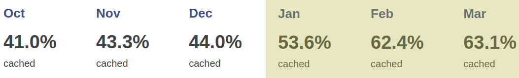
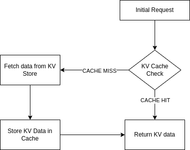
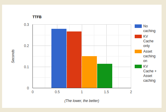


")

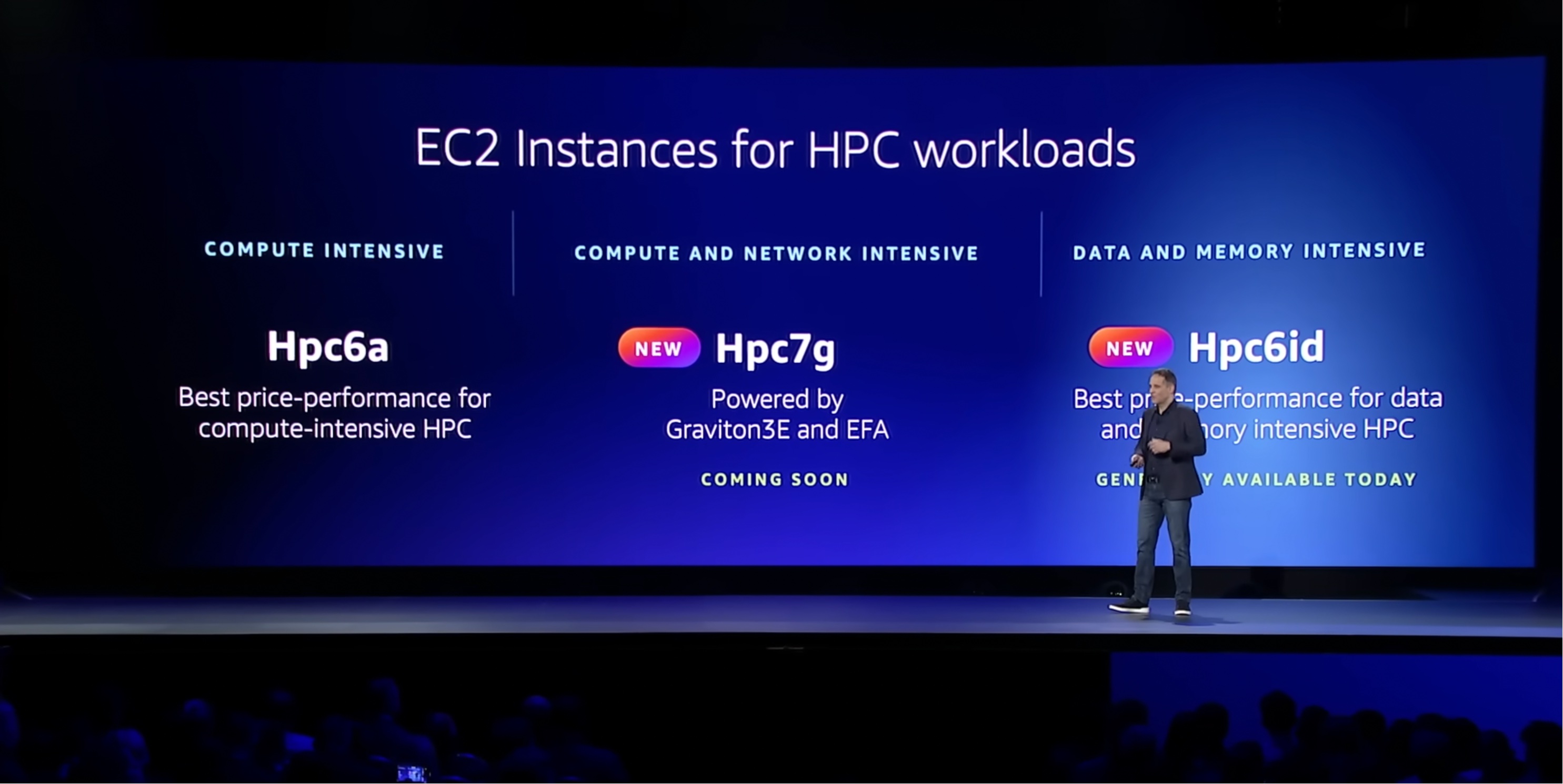
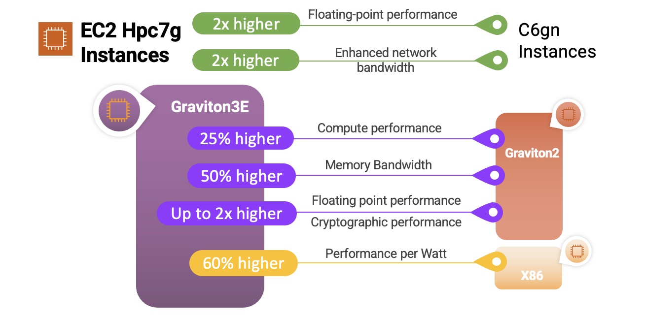


 Chaitanya Shah is a Sr. Technical Account Manager(TAM) with AWS, based out of New York. He has over 22 years of experience working with enterprise customers. He loves to code and actively contributes to the AWS solutions labs to help customers solve complex problems. He provides guidance to AWS customers on best practices for their AWS Cloud migrations. He is also specialized in AWS data transfer and the data and analytics domain.


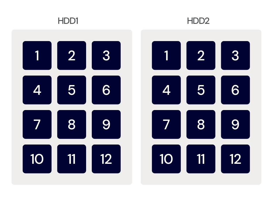
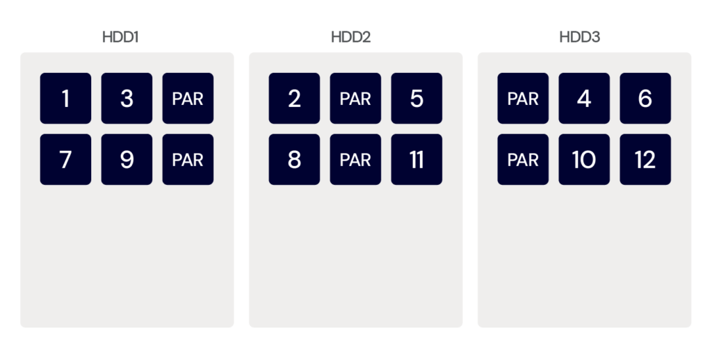
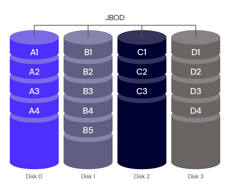
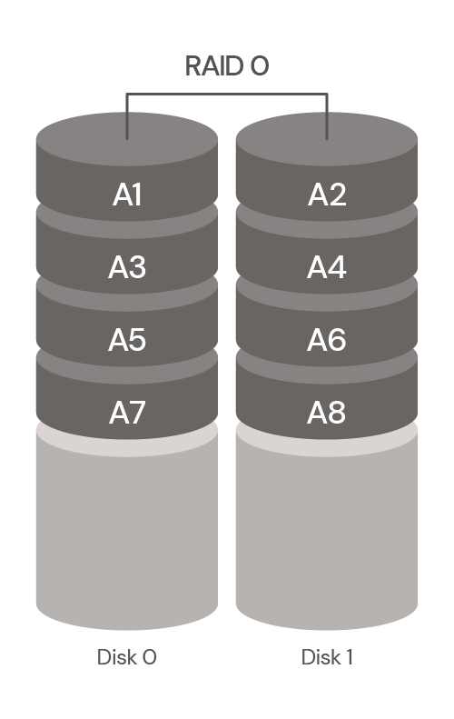
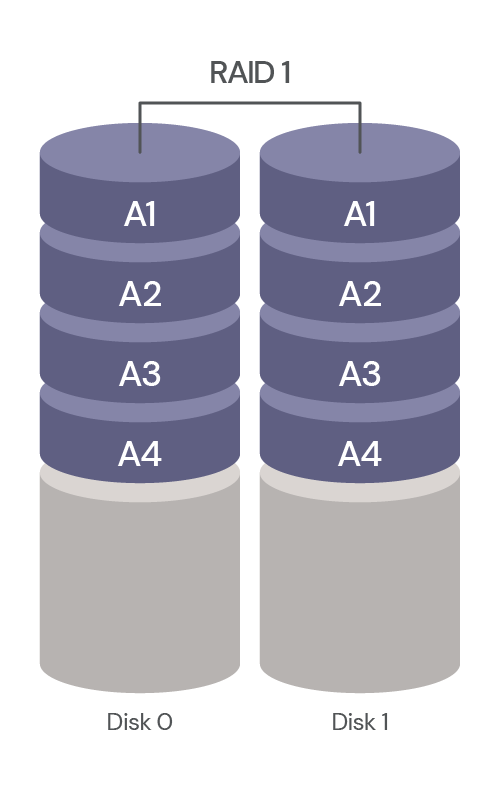
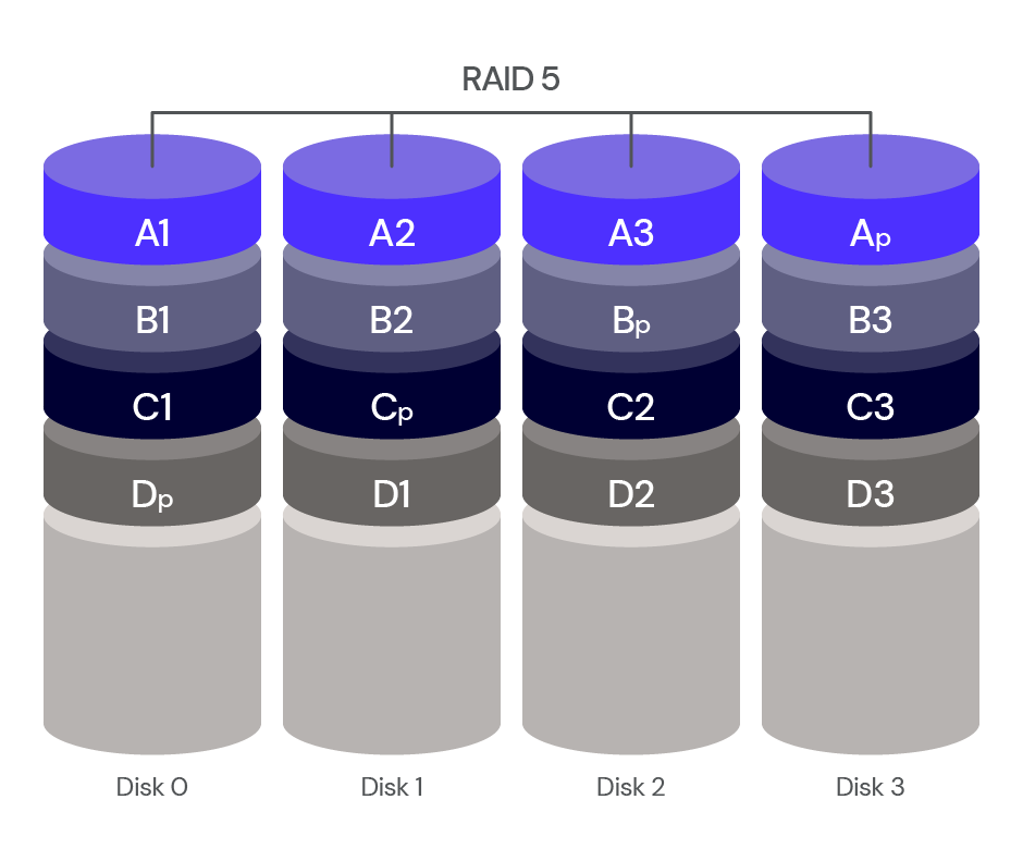
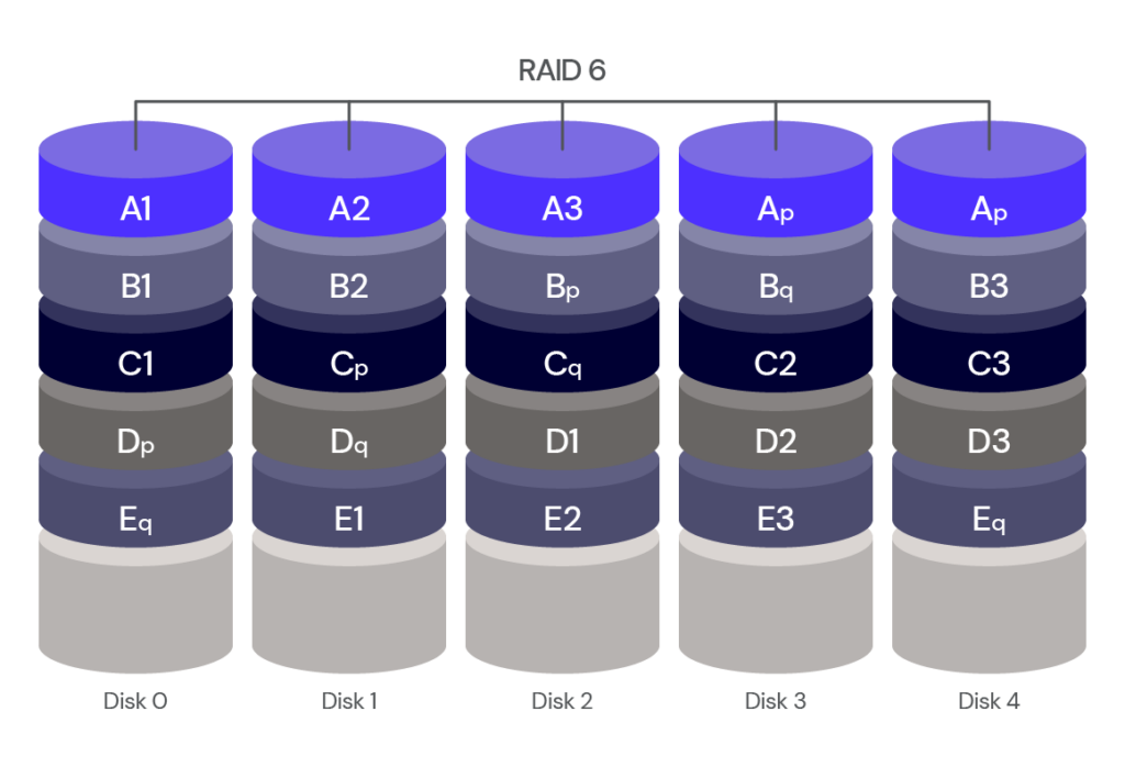
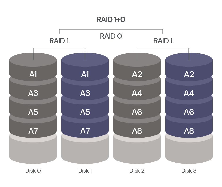
 usando p5.js, uma biblioteca JavaScript para código criativo, continuamos recebendo sugestões irrelevantes ou, às vezes, nenhuma sugestão. Mas quando aprendemos mais sobre a maneira como o GitHub Copilot processa as informações, percebemos que precisávamos ajustar a maneira como nos comunicamos com elas.
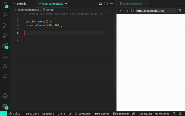


 de práctica