How the GoDaddy data platform achieved over 60% cost reduction and 50% performance boost by adopting Amazon EMR Serverless

Post Syndicated from Brandon Abear original https://aws.amazon.com/blogs/big-data/how-the-godaddy-data-platform-achieved-over-60-cost-reduction-and-50-performance-boost-by-adopting-amazon-emr-serverless/

This is a guest post co-written with Brandon Abear, Dinesh Sharma, John Bush, and Ozcan IIikhan from GoDaddy.

GoDaddy empowers everyday entrepreneurs by providing all the help and tools to succeed online. With more than 20 million customers worldwide, GoDaddy is the place people come to name their ideas, build a professional website, attract customers, and manage their work.

At GoDaddy, we take pride in being a data-driven company. Our relentless pursuit of valuable insights from data fuels our business decisions and ensures customer satisfaction. Our commitment to efficiency is unwavering, and we’ve undertaken an exciting initiative to optimize our batch processing jobs. In this journey, we have identified a structured approach that we refer to as the seven layers of improvement opportunities. This methodology has become our guide in the pursuit of efficiency.

In this post, we discuss how we enhanced operational efficiency with Amazon EMR Serverless. We share our benchmarking results and methodology, and insights into the cost-effectiveness of EMR Serverless vs. fixed capacity Amazon EMR on EC2 transient clusters on our data workflows orchestrated using Amazon Managed Workflows for Apache Airflow (Amazon MWAA). We share our strategy for the adoption of EMR Serverless in areas where it excels. Our findings reveal significant benefits, including over 60% cost reduction, 50% faster Spark workloads, a remarkable five-times improvement in development and testing speed, and a significant reduction in our carbon footprint.

Background

In late 2020, GoDaddy’s data platform initiated its AWS Cloud journey, migrating an 800-node Hadoop cluster with 2.5 PB of data from its data center to EMR on EC2. This lift-and-shift approach facilitated a direct comparison between on-premises and cloud environments, ensuring a smooth transition to AWS pipelines, minimizing data validation issues and migration delays.

By early 2022, we successfully migrated our big data workloads to EMR on EC2. Using best practices learned from the AWS FinHack program, we fine-tuned resource-intensive jobs, converted Pig and Hive jobs to Spark, and reduced our batch workload spend by 22.75% in 2022. However, scalability challenges emerged due to the multitude of jobs. This prompted GoDaddy to embark on a systematic optimization journey, establishing a foundation for more sustainable and efficient big data processing.

Seven layers of improvement opportunities

In our quest for operational efficiency, we have identified seven distinct layers of opportunities for optimization within our batch processing jobs, as shown in the following figure. These layers range from precise code-level enhancements to more comprehensive platform improvements. This multi-layered approach has become our strategic blueprint in the ongoing pursuit of better performance and higher efficiency.

Seven layers of improvement opportunities

The layers are as follows:

  • Code optimization – Focuses on refining the code logic and how it can be optimized for better performance. This involves performance enhancements through selective caching, partition and projection pruning, join optimizations, and other job-specific tuning. Using AI coding solutions is also an integral part of this process.
  • Software updates – Updating to the latest versions of open source software (OSS) to capitalize on new features and improvements. For example, Adaptive Query Execution in Spark 3 brings significant performance and cost improvements.
  • Custom Spark configurations – Tuning of custom Spark configurations to maximize resource utilization, memory, and parallelism. We can achieve significant improvements by right-sizing tasks, such as through spark.sql.shuffle.partitions, spark.sql.files.maxPartitionBytes, spark.executor.cores, and spark.executor.memory. However, these custom configurations might be counterproductive if they are not compatible with the specific Spark version.
  • Resource provisioning time – The time it takes to launch resources like ephemeral EMR clusters on Amazon Elastic Compute Cloud (Amazon EC2). Although some factors influencing this time are outside of an engineer’s control, identifying and addressing the factors that can be optimized can help reduce overall provisioning time.
  • Fine-grained scaling at task level – Dynamically adjusting resources such as CPU, memory, disk, and network bandwidth based on each stage’s needs within a task. The aim here is to avoid fixed cluster sizes that could result in resource waste.
  • Fine-grained scaling across multiple tasks in a workflow – Given that each task has unique resource requirements, maintaining a fixed resource size may result in under- or over-provisioning for certain tasks within the same workflow. Traditionally, the size of the largest task determines the cluster size for a multi-task workflow. However, dynamically adjusting resources across multiple tasks and steps within a workflow result in a more cost-effective implementation.
  • Platform-level enhancements – Enhancements at preceding layers can only optimize a given job or a workflow. Platform improvement aims to attain efficiency at the company level. We can achieve this through various means, such as updating or upgrading the core infrastructure, introducing new frameworks, allocating appropriate resources for each job profile, balancing service usage, optimizing the use of Savings Plans and Spot Instances, or implementing other comprehensive changes to boost efficiency across all tasks and workflows.

Layers 1–3: Previous cost reductions

After we migrated from on premises to AWS Cloud, we primarily focused our cost-optimization efforts on the first three layers shown in the diagram. By transitioning our most costly legacy Pig and Hive pipelines to Spark and optimizing Spark configurations for Amazon EMR, we achieved significant cost savings.

For example, a legacy Pig job took 10 hours to complete and ranked among the top 10 most expensive EMR jobs. Upon reviewing TEZ logs and cluster metrics, we discovered that the cluster was vastly over-provisioned for the data volume being processed and remained under-utilized for most of the runtime. Transitioning from Pig to Spark was more efficient. Although no automated tools were available for the conversion, manual optimizations were made, including:

  • Reduced unnecessary disk writes, saving serialization and deserialization time (Layer 1)
  • Replaced Airflow task parallelization with Spark, simplifying the Airflow DAG (Layer 1)
  • Eliminated redundant Spark transformations (Layer 1)
  • Upgraded from Spark 2 to 3, using Adaptive Query Execution (Layer 2)
  • Addressed skewed joins and optimized smaller dimension tables (Layer 3)

As a result, job cost decreased by 95%, and job completion time was reduced to 1 hour. However, this approach was labor-intensive and not scalable for numerous jobs.

Layers 4–6: Find and adopt the right compute solution

In late 2022, following our significant accomplishments in optimization at the previous levels, our attention moved towards enhancing the remaining layers.

Understanding the state of our batch processing

We use Amazon MWAA to orchestrate our data workflows in the cloud at scale. Apache Airflow is an open source tool used to programmatically author, schedule, and monitor sequences of processes and tasks referred to as workflows. In this post, the terms workflow and job are used interchangeably, referring to the Directed Acyclic Graphs (DAGs) consisting of tasks orchestrated by Amazon MWAA. For each workflow, we have sequential or parallel tasks, and even a combination of both in the DAG between create_emr and terminate_emr tasks running on a transient EMR cluster with fixed compute capacity throughout the workflow run. Even after optimizing a portion of our workload, we still had numerous non-optimized workflows that were under-utilized due to over-provisioning of compute resources based on the most resource-intensive task in the workflow, as shown in the following figure.

This highlighted the impracticality of static resource allocation and led us to recognize the necessity of a dynamic resource allocation (DRA) system. Before proposing a solution, we gathered extensive data to thoroughly understand our batch processing. Analyzing the cluster step time, excluding provisioning and idle time, revealed significant insights: a right-skewed distribution with over half of the workflows completing in 20 minutes or less and only 10% taking more than 60 minutes. This distribution guided our choice of a fast-provisioning compute solution, dramatically reducing workflow runtimes. The following diagram illustrates step times (excluding provisioning and idle time) of EMR on EC2 transient clusters in one of our batch processing accounts.

Furthermore, based on the step time (excluding provisioning and idle time) distribution of the workflows, we categorized our workflows into three groups:

  • Quick run – Lasting 20 minutes or less
  • Medium run – Lasting between 20–60 minutes
  • Long run – Exceeding 60 minutes, often spanning several hours or more

Another factor we needed to consider was the extensive use of transient clusters for reasons such as security, job and cost isolation, and purpose-built clusters. Additionally, there was a significant variation in resource needs between peak hours and periods of low utilization.

Instead of fixed-size clusters, we could potentially use managed scaling on EMR on EC2 to achieve some cost benefits. However, migrating to EMR Serverless appears to be a more strategic direction for our data platform. In addition to potential cost benefits, EMR Serverless offers additional advantages such as a one-click upgrade to the newest Amazon EMR versions, a simplified operational and debugging experience, and automatic upgrades to the latest generations upon rollout. These features collectively simplify the process of operating a platform on a larger scale.

Evaluating EMR Serverless: A case study at GoDaddy

EMR Serverless is a serverless option in Amazon EMR that eliminates the complexities of configuring, managing, and scaling clusters when running big data frameworks like Apache Spark and Apache Hive. With EMR Serverless, businesses can enjoy numerous benefits, including cost-effectiveness, faster provisioning, simplified developer experience, and improved resilience to Availability Zone failures.

Recognizing the potential of EMR Serverless, we conducted an in-depth benchmark study using real production workflows. The study aimed to assess EMR Serverless performance and efficiency while also creating an adoption plan for large-scale implementation. The findings were highly encouraging, showing EMR Serverless can effectively handle our workloads.

Benchmarking methodology

We split our data workflows into three categories based on total step time (excluding provisioning and idle time): quick run (0–20 minutes), medium run (20–60 minutes), and long run (over 60 minutes). We analyzed the impact of the EMR deployment type (Amazon EC2 vs. EMR Serverless) on two key metrics: cost-efficiency and total runtime speedup, which served as our overall evaluation criteria. Although we did not formally measure ease of use and resiliency, these factors were considered throughout the evaluation process.

The high-level steps to assess the environment are as follows:

  1. Prepare the data and environment:
    1. Choose three to five random production jobs from each job category.
    2. Implement required adjustments to prevent interference with production.
  2. Run tests:
    1. Run scripts over several days or through multiple iterations to gather precise and consistent data points.
    2. Perform tests using EMR on EC2 and EMR Serverless.
  3. Validate data and test runs:
    1. Validate input and output datasets, partitions, and row counts to ensure identical data processing.
  4. Gather metrics and analyze results:
    1. Gather relevant metrics from the tests.
    2. Analyze results to draw insights and conclusions.

Benchmark results

Our benchmark results showed significant enhancements across all three job categories for both runtime speedup and cost-efficiency. The improvements were most pronounced for quick jobs, directly resulting from faster startup times. For instance, a 20-minute (including cluster provisioning and shut down) data workflow running on an EMR on EC2 transient cluster of fixed compute capacity finishes in 10 minutes on EMR Serverless, providing a shorter runtime with cost benefits. Overall, the shift to EMR Serverless delivered substantial performance improvements and cost reductions at scale across job brackets, as seen in the following figure.

Historically, we devoted more time to tuning our long-run workflows. Interestingly, we discovered that the existing custom Spark configurations for these jobs did not always translate well to EMR Serverless. In cases where the results were insignificant, a common approach was to discard previous Spark configurations related to executor cores. By allowing EMR Serverless to autonomously manage these Spark configurations, we often observed improved outcomes. The following graph shows the average runtime and cost improvement per job when comparing EMR Serverless to EMR on EC2.

Per Job Improvement

The following table shows a sample comparison of results for the same workflow running on different deployment options of Amazon EMR (EMR on EC2 and EMR Serverless).

Metric EMR on EC2
(Average)
EMR Serverless
(Average)
EMR on EC2 vs
EMR Serverless
Total Run Cost ($) $ 5.82 $ 2.60 55%
Total Run Time (Minutes) 53.40 39.40 26%
Provisioning Time (Minutes) 10.20 0.05 .
Provisioning Cost ($) $ 1.19 . .
Steps Time (Minutes) 38.20 39.16 -3%
Steps Cost ($) $ 4.30 . .
Idle Time (Minutes) 4.80 . .
EMR Release Label emr-6.9.0 .
Hadoop Distribution Amazon 3.3.3 .
Spark Version Spark 3.3.0 .
Hive/HCatalog Version Hive 3.1.3, HCatalog 3.1.3 .
Job Type Spark .

AWS Graviton2 on EMR Serverless performance evaluation

After seeing compelling results with EMR Serverless for our workloads, we decided to further analyze the performance of the AWS Graviton2 (arm64) architecture within EMR Serverless. AWS had benchmarked Spark workloads on Graviton2 EMR Serverless using the TPC-DS 3TB scale, showing a 27% overall price-performance improvement.

To better understand the integration benefits, we ran our own study using GoDaddy’s production workloads on a daily schedule and observed an impressive 23.8% price-performance enhancement across a range of jobs when using Graviton2. For more details about this study, see GoDaddy benchmarking results in up to 24% better price-performance for their Spark workloads with AWS Graviton2 on Amazon EMR Serverless.

Adoption strategy for EMR Serverless

We strategically implemented a phased rollout of EMR Serverless via deployment rings, enabling systematic integration. This gradual approach let us validate improvements and halt further adoption of EMR Serverless, if needed. It served both as a safety net to catch issues early and a means to refine our infrastructure. The process mitigated change impact through smooth operations while building team expertise of our Data Engineering and DevOps teams. Additionally, it fostered tight feedback loops, allowing prompt adjustments and ensuring efficient EMR Serverless integration.

We divided our workflows into three main adoption groups, as shown in the following image:

  • Canaries – This group aids in detecting and resolving any potential problems early in the deployment stage.
  • Early adopters – This is the second batch of workflows that adopt the new compute solution after initial issues have been identified and rectified by the canaries group.
  • Broad deployment rings – The largest group of rings, this group represents the wide-scale deployment of the solution. These are deployed after successful testing and implementation in the previous two groups.

Rings

We further broke down these workflows into granular deployment rings to adopt EMR Serverless, as shown in the following table.

Ring # Name Details
Ring 0 Canary Low adoption risk jobs that are expected to yield some cost saving benefits.
Ring 1 Early Adopters Low risk Quick-run Spark jobs that expect to yield high gains.
Ring 2 Quick-run Rest of the Quick-run (step_time <= 20 min) Spark jobs
Ring 3 LargerJobs_EZ High potential gain, easy move, medium-run and long-run Spark jobs
Ring 4 LargerJobs Rest of the medium-run and long-run Spark jobs with potential gains
Ring 5 Hive Hive jobs with potentially higher cost savings
Ring 6 Redshift_EZ Easy migration Redshift jobs that suit EMR Serverless
Ring 7 Glue_EZ Easy migration Glue jobs that suit EMR Serverless

Production adoption results summary

The encouraging benchmarking and canary adoption results generated considerable interest in wider EMR Serverless adoption at GoDaddy. To date, the EMR Serverless rollout remains underway. Thus far, it has reduced costs by 62.5% and accelerated total batch workflow completion by 50.4%.

Based on preliminary benchmarks, our team expected substantial gains for quick jobs. To our surprise, actual production deployments surpassed projections, averaging 64.4% faster vs. 42% projected, and 71.8% cheaper vs. 40% predicted.

Remarkably, long-running jobs also saw significant performance improvements due to the rapid provisioning of EMR Serverless and aggressive scaling enabled by dynamic resource allocation. We observed substantial parallelization during high-resource segments, resulting in a 40.5% faster total runtime compared to traditional approaches. The following chart illustrates the average enhancements per job category.

Prod Jobs Savings

Additionally, we observed the highest degree of dispersion for speed improvements within the long-run job category, as shown in the following box-and-whisker plot.

Whisker Plot

Sample workflows adopted EMR Serverless

For a large workflow migrated to EMR Serverless, comparing 3-week averages pre- and post-migration revealed impressive cost savings—a 75.30% decrease based on retail pricing with 10% improvement in total runtime, boosting operational efficiency. The following graph illustrates the cost trend.

Although quick-run jobs realized minimal per-dollar cost reductions, they delivered the most significant percentage cost savings. With thousands of these workflows running daily, the accumulated savings are substantial. The following graph shows the cost trend for a small workload migrated from EMR on EC2 to EMR Serverless. Comparing 3-week pre- and post-migration averages revealed a remarkable 92.43% cost savings on the retail on-demand pricing, alongside an 80.6% acceleration in total runtime.

Sample workflows adopted EMR Serverless 2

Layer 7: Platform-wide improvements

We aim to revolutionize compute operations at GoDaddy, providing simplified yet powerful solutions for all users with our Intelligent Compute Platform. With AWS compute solutions like EMR Serverless and EMR on EC2, it provided optimized runs of data processing and machine learning (ML) workloads. An ML-powered job broker intelligently determines when and how to run jobs based on various parameters, while still allowing power users to customize. Additionally, an ML-powered compute resource manager pre-provisions resources based on load and historical data, providing efficient, fast provisioning at optimum cost. Intelligent compute empowers users with out-of-the-box optimization, catering to diverse personas without compromising power users.

The following diagram shows a high-level illustration of the intelligent compute architecture.

Insights and recommended best-practices

The following section discusses the insights we’ve gathered and the recommended best practices we’ve developed during our preliminary and wider adoption stages.

Infrastructure preparation

Although EMR Serverless is a deployment method within EMR, it requires some infrastructure preparedness to optimize its potential. Consider the following requirements and practical guidance on implementation:

  • Use large subnets across multiple Availability Zones – When running EMR Serverless workloads within your VPC, make sure the subnets span across multiple Availability Zones and are not constrained by IP addresses. Refer to Configuring VPC access and Best practices for subnet planning for details.
  • Modify maximum concurrent vCPU quota – For extensive compute requirements, it is recommended to increase your max concurrent vCPUs per account service quota.
  • Amazon MWAA version compatibility – When adopting EMR Serverless, GoDaddy’s decentralized Amazon MWAA ecosystem for data pipeline orchestration created compatibility issues from disparate AWS Providers versions. Directly upgrading Amazon MWAA was more efficient than updating numerous DAGs. We facilitated adoption by upgrading Amazon MWAA instances ourselves, documenting issues, and sharing findings and effort estimates for accurate upgrade planning.
  • GoDaddy EMR operator – To streamline migrating numerous Airflow DAGs from EMR on EC2 to EMR Serverless, we developed custom operators adapting existing interfaces. This allowed seamless transitions while retaining familiar tuning options. Data engineers could easily migrate pipelines with simple find-replace imports and immediately use EMR Serverless.

Unexpected behavior mitigation

The following are unexpected behaviors we ran into and what we did to mitigate them:

  • Spark DRA aggressive scaling – For some jobs (8.33% of initial benchmarks, 13.6% of production), cost increased after migrating to EMR Serverless. This was due to Spark DRA excessively assigning new workers briefly, prioritizing performance over cost. To counteract this, we set maximum executor thresholds by adjusting spark.dynamicAllocation.maxExecutor, effectively limiting EMR Serverless scaling aggression. When migrating from EMR on EC2, we suggest observing the max core count in the Spark History UI to replicate similar compute limits in EMR Serverless, such as --conf spark.executor.cores and --conf spark.dynamicAllocation.maxExecutors.
  • Managing disk space for large-scale jobs – When transitioning jobs that process large data volumes with substantial shuffles and significant disk requirements to EMR Serverless, we recommend configuring spark.emr-serverless.executor.disk by referring to existing Spark job metrics. Furthermore, configurations like spark.executor.cores combined with spark.emr-serverless.executor.disk and spark.dynamicAllocation.maxExecutors allow control over the underlying worker size and total attached storage when advantageous. For example, a shuffle-heavy job with relatively low disk usage may benefit from using a larger worker to increase the likelihood of local shuffle fetches.

Conclusion

As discussed in this post, our experiences with adopting EMR Serverless on arm64 have been overwhelmingly positive. The impressive results we’ve achieved, including a 60% reduction in cost, 50% faster runs of batch Spark workloads, and an astounding five-times improvement in development and testing speed, speak volumes about the potential of this technology. Furthermore, our current results suggest that by widely adopting Graviton2 on EMR Serverless, we could potentially reduce the carbon footprint by up to 60% for our batch processing.

However, it’s crucial to understand that these results are not a one-size-fits-all scenario. The enhancements you can expect are subject to factors including, but not limited to, the specific nature of your workflows, cluster configurations, resource utilization levels, and fluctuations in computational capacity. Therefore, we strongly advocate for a data-driven, ring-based deployment strategy when considering the integration of EMR Serverless, which can help optimize its benefits to the fullest.

Special thanks to Mukul Sharma and Boris Berlin for their contributions to benchmarking. Many thanks to Travis Muhlestein (CDO), Abhijit Kundu (VP Eng), Vincent Yung (Sr. Director Eng.), and Wai Kin Lau (Sr. Director Data Eng.) for their continued support.


About the Authors

Brandon Abear is a Principal Data Engineer in the Data & Analytics (DnA) organization at GoDaddy. He enjoys all things big data. In his spare time, he enjoys traveling, watching movies, and playing rhythm games.

Dinesh Sharma is a Principal Data Engineer in the Data & Analytics (DnA) organization at GoDaddy. He is passionate about user experience and developer productivity, always looking for ways to optimize engineering processes and saving cost. In his spare time, he loves reading and is an avid manga fan.

John Bush is a Principal Software Engineer in the Data & Analytics (DnA) organization at GoDaddy. He is passionate about making it easier for organizations to manage data and use it to drive their businesses forward. In his spare time, he loves hiking, camping, and riding his ebike.

Ozcan Ilikhan is the Director of Engineering for the Data and ML Platform at GoDaddy. He has over two decades of multidisciplinary leadership experience, spanning startups to global enterprises. He has a passion for leveraging data and AI in creating solutions that delight customers, empower them to achieve more, and boost operational efficiency. Outside of his professional life, he enjoys reading, hiking, gardening, volunteering, and embarking on DIY projects.

Harsh Vardhan is an AWS Solutions Architect, specializing in big data and analytics. He has over 8 years of experience working in the field of big data and data science. He is passionate about helping customers adopt best practices and discover insights from their data.
[$] Insecurity and Python pickles

Post Syndicated from daroc original https://lwn.net/Articles/964392/

Serialization is the process of transforming Python objects into a sequence of
bytes which can be used to recreate a copy of the object later — or on another
machine.

pickle
is Python’s native serialization module. It can store complex Python
objects,
making it an appealing prospect for moving data without having to write
custom serialization code. For example, pickle is an integral component of
several file
formats
used for machine learning. However, using pickle to deserialize
untrusted files is a major security risk, because doing so can invoke arbitrary
Python functions. Consequently, the machine-learning community is working to address the
security issues caused by widespread use of pickle.

Security updates for Tuesday

Post Syndicated from corbet original https://lwn.net/Articles/965113/

Security updates have been issued by Debian (qemu), Mageia (libtiff and thunderbird), Red Hat (kernel, kpatch-patch, postgresql, and rhc-worker-script), SUSE (compat-openssl098, openssl, openssl1, python-Django, python-Django1, and wpa_supplicant), and Ubuntu (accountsservice, libxml2, linux-bluefield, linux-raspi-5.4, linux-xilinx-zynqmp, linux-oem-6.1, openvswitch, postgresql-9.5, and ruby-rack).

Huston: KeyTrap!

Post Syndicated from corbet original https://lwn.net/Articles/965067/

Geoff Huston digs into the
details
of the KeyTrap DNS vulnerability, which was disclosed in February.

It’s by no means “devasting” for the DNS, and the fix is much the
same as the previous fix. As well as limiting the number of queries
that a resolver can generate to resolve a queried name, a careful
resolver will limit both the elapsed time and perhaps the amount of
the resolver’s processing resources that are used to resolve any
single query name.

It’s also not a novel discovery by the ATHENE folk. The
vulnerability was described five years ago by a student at the
University of Twente. I guess the issue was that the student failed
to use a sufficient number of hysterical adjectives in describing
this DNS vulnerability in the paper!

Physics on AWS: Optimizing wind turbine performance using OpenFAST in a digital twin

Post Syndicated from Marco Masciola original https://aws.amazon.com/blogs/architecture/physics-on-aws-optimizing-wind-turbine-performance-using-openfast-in-a-digital-twin/

Wind energy plays a crucial role in global decarbonization efforts by generating emission-free power from an abundant resource. In 2022, wind energy produced 2100 terawatt-hours (TWh) globally, or over 7% of global electricity, with expectations to reach 7400 TWh by 2030.

Despite its potential, several challenges must be addressed to help meet grid decarbonization targets. As wind energy adoption grows, issues like gearbox fatigue and leading-edge erosion need to be resolved to ensure a predictable supply of energy. For example, in the United States, wind turbines underperform by as much as 10% after 11 years of operation, despite expectations for the machine to operate at full potential for 25 years.

This blog reveals a digital twin architecture using the National Renewable Energy Laboratory’s (NREL) OpenFAST, an open-source multi-physics wind turbine simulation tool, to characterize operational anomalies and continuously improve wind farm performance. This approach can be used to support an overall maintenance strategy to optimize performance and profitability while reducing risk.

While a digital twin can take many forms, this architecture represents it with a physical wind turbine connected to the cloud using IoT devices to monitor performance and augmented knowledge using on-demand simulations. The insight gained from simulations can update the physical asset control system in near real-time to balance operational performance.

Why build this?

This digital twin can catch reliability assessment discrepancies by benchmarking real-world time series with simulations. Aeroelastic simulators like OpenFAST define operational envelopes as part of wind turbine design and certification in accordance with IEC 61400-1 and 61400-3. However, subtle, unanticipated changes in environmental conditions not accounted for in the initial design certification, such as higher turbulence intensity, accelerate degradation.

This architecture can be used to validate if a controller change can limit gradual performance damage before the controller changes are deployed by using the same simulation software for wind turbine design. This example scenario, one that operators currently struggle with, is threaded in the next section.

Digital twin architecture

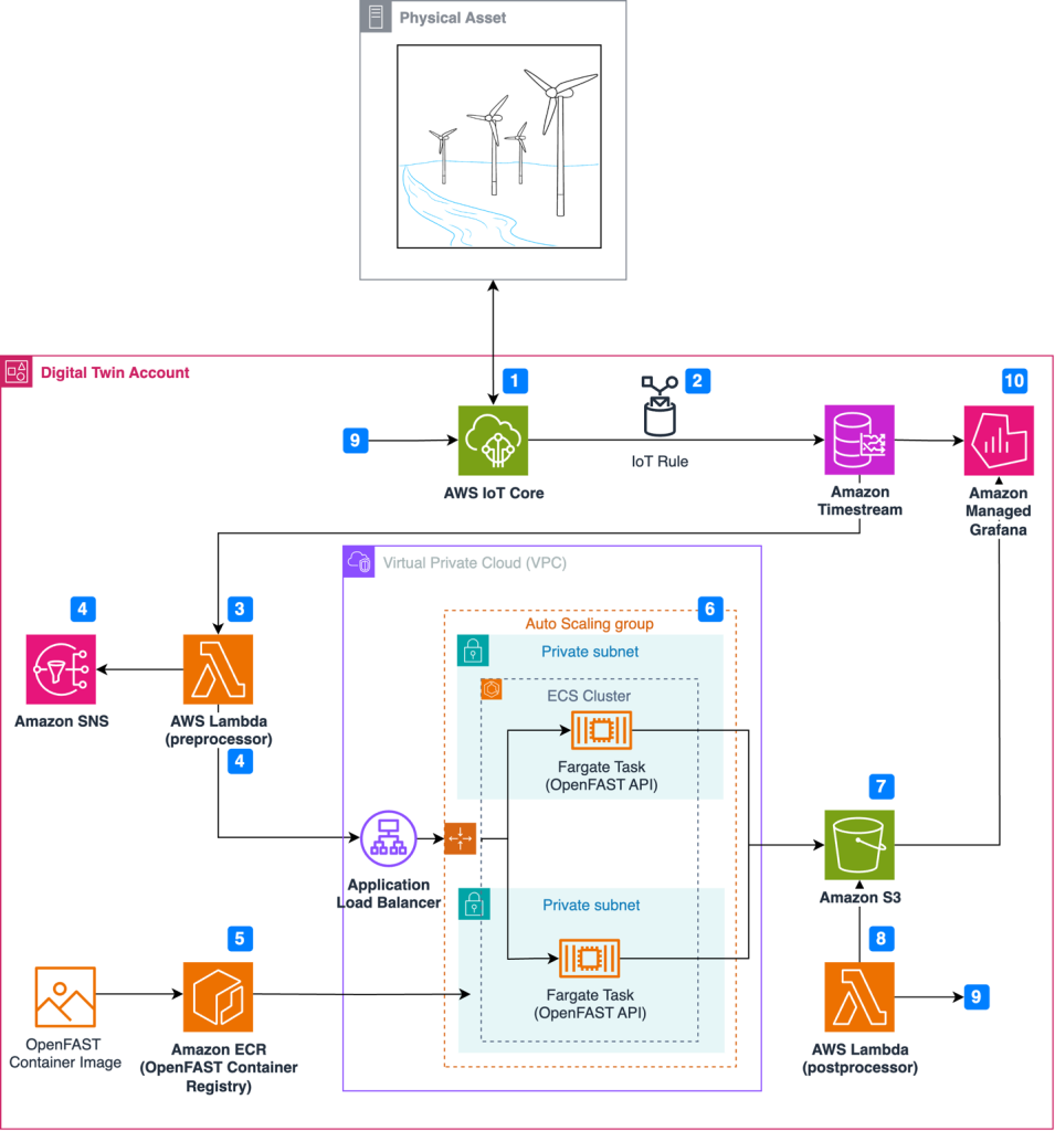
Figure 1 illustrates the event-driven architecture in which resources launch on-demand simulations as anomalies occur.

Architecture for wind turbine digital twin solution

Figure 1. Architecture for wind turbine digital twin solution

Simulation and real-world results can feed into a calculation engine to update the wind turbine controller software and improve operational performance through this workflow:

  1. Wind turbine sensors are connected to the AWS cloud using AWS IoT Core.
  2. An IoT rule forwards sensor data to Amazon Timestream, a purpose-built time series database.
  3. A scheduled AWS Lambda function queries Timestream to detect anomalies in time-series data.
  4. Upon anomaly detection, Amazon Simple Notification Service (Amazon SNS) publishes notifications and OpenFAST simulation input files are prepared in the Lambda preprocessor.
  5. Simulations are executed on demand, where the latest OpenFAST simulation is pulled from Amazon Elastic Container Registry (Amazon ECR).
  6. Simulations are dispatched through RESTful API and run using AWS Fargate.
  7. Simulation results are uploaded to Amazon Simple Storage Service (Amazon S3).
  8. Simulation time-series data is processed using AWS Lambda, where a decision is made to update the controller software based on the anomaly.
  9. The Lambda post-processer initiates a wind turbine controller software update, which is communicated to the wind turbine through AWS IoT Core.
  10. Results are visualized in Amazon Managed Grafana.

An example of an anomaly in step 3 is a controller overspeed alarm. Simple rule-based anomaly detection can be used to detect exceedance thresholds. You can also incorporate more sophisticated forms of anomaly detection using machine learning through Amazon SageMaker. The workflow above preserves four elements to create a digital twin. We will explore these four elements in the next section:

Event-driven architecture

Event-driven architectures enable decoupled systems and asynchronous communications between services. An event-driven workflow is initiated automatically as events occur. An event might be an active alarm or an OpenFAST output file uploaded to Amazon S3. This means that the number of actively monitored wind turbines can scale from one to 100 (or more) without allocating new resources.

AWS Lambda provides instant scaling to increase the number of OpenFAST simulations available for processing. Additionally, Fargate removes the need to provision or manage the underlying OpenFAST compute instances. Leveraging serverless compute services removes the need to manage underlying infrastructure, provides demand-based scaling, and reduces costs compared to statically provisioned infrastructure.

In practice, event-driven architecture provides teams with flexibility to automatically prepare input files, dispatch simulations, and post-process results without manually provisioning resources.

Containerization

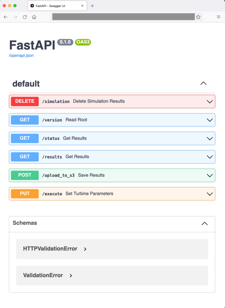
Containerization is a process to deploy an application with libraries needed for execution. Docker creates a container image that bundles the OpenFAST executable. FastAPI is also included in the OpenFAST container so that simulations can be dispatched through a web RESTful API, as demonstrated in Figure 2. Note that OpenFAST and FastAPI are independent projects. The RESTful API for OpenFAST is provisioned with commands to:

  • Run the simulation with initial conditions (PUT: /execute)
  • Upload simulation results to Amazon S3 (POST: /upload_to_s3)
  • Provide simulation status (GET: /status)
  • Delete simulation results (DELETE: /simulation)

This setup enables engineering teams to pull an OpenFAST simulation version aligned with physical wind turbines in operation without manual configuration.

Web frontend showing the RESTfulAPI commands available for dispatching OpenFAST simulations

Figure 2. Web frontend showing the RESTfulAPI commands available for dispatching OpenFAST simulations

Load balancing and auto scaling

The architecture uses Amazon EC2 Auto Scaling and an ALB to manage fluctuating processing demands and enable concurrent OpenFAST simulations. EC2 Auto Scaling dynamically scales the number of OpenFAST containers based on the volume of simulation requests and offers cost savings to avoid idle resources. Paired with an ALB, this setup evenly distributes simulation requests across OpenFAST containers, ensuring desired performance levels and high availability.

Data visualization

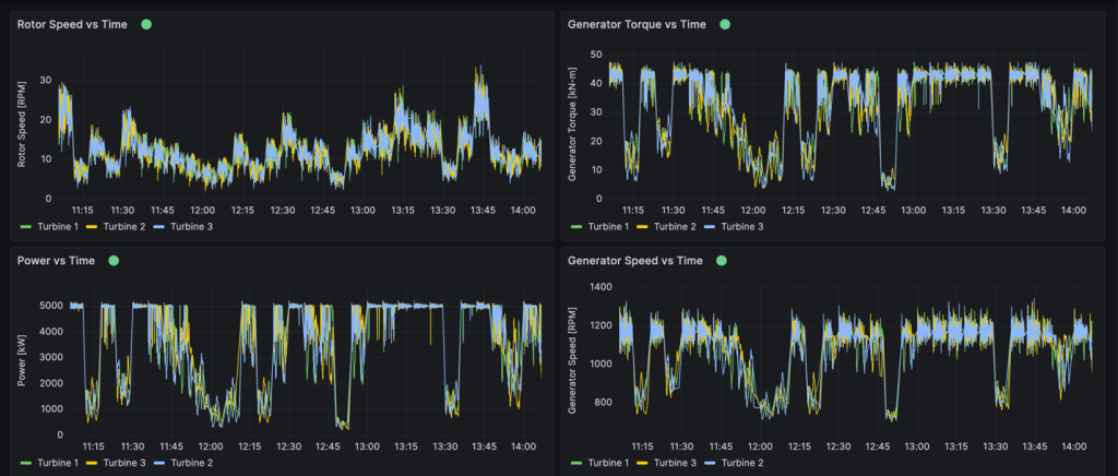
Amazon Timestream collects and archives real-time metrics from physical wind turbines. Timestream can store any metric from the physical asset collected through IoT Core, including rotor speed, generator power, generator speed, generator torque, or wind turbine control system alarms, as shown in Figure 3. One distinctive Timestream feature is scheduled queries that can regularly perform automated tasks like measuring 10-minute average wind speeds or tracking down units with controller alarms.

This provides operations teams the ability to view granular insights in real time or query historical data using SQL. Amazon Managed Grafana is also connected to OpenFAST results stored in Amazon S3 to compare simulation results with real-world operational data and view the response of simulated components. Engineering teams benefit from Amazon Managed Grafana because it provides a window into how the simulation responds to controller changes. Engineers can then verify whether the physical machine responds in the expected manner.

Example Amazon Managed Grafana dashboard

Figure 3. Example Amazon Managed Grafana dashboard

Conclusion

The AWS Cloud offers services and infrastructure to provide organization resources to process data and build digital twins. Organizations can leverage open-source models to improve operational performance and physics-based simulations to improve accuracy. By integrating technology paradigms such as event-drive architectures, wind turbine operators can make data-driven decisions in real time. Organizations can create virtual replicas of physical wind turbines to diagnose the source of alarms and adopt strategies to limit excessive wear before permanent damage occurs.

AWS Wickr achieves FedRAMP High authorization

Post Syndicated from Anne Grahn original https://aws.amazon.com/blogs/security/aws-wickr-achieves-fedramp-high-authorization/

Amazon Web Services (AWS) is excited to announce that AWS Wickr has achieved Federal Risk and Authorization Management Program (FedRAMP) authorization at the High impact level from the FedRAMP Joint Authorization Board (JAB).

FedRAMP is a U.S. government–wide program that promotes the adoption of secure cloud services by providing a standardized approach to security and risk assessment for cloud technologies and federal agencies.

Customers find security and control in Wickr

Wickr is an end-to-end encrypted messaging and collaboration service with features designed to help keep your communications secure, private, and compliant. Wickr protects one-to-one and group messaging, voice and video calling, file sharing, screen sharing, and location sharing with 256-bit encryption, and provides data retention capabilities.

You can create Wickr networks through the AWS Management Console. Administrative controls allow your Wickr administrators to add, remove, and invite users, and organize them into security groups to manage messaging, calling, security, and federation settings. You maintain full control over data, which includes addressing information governance polices, configuring ephemeral messaging options, and deleting credentials for lost or stolen devices.

You can log internal and external communications—including conversations with guest users, contractors, and other partner networks—in a private data store that you manage. This allows you to retain messages and files that are sent to and from your organization, to help meet requirements such as those that fall under the Federal Records Act (FRA) and the National Archives and Records Administration (NARA).

The FedRAMP milestone

In obtaining a FedRAMP High authorization, Wickr has been measured against a rigorous set of security controls, procedures, and policies established by the U.S. Federal Government, based on National Institute of Standards and Technology (NIST) standards.

“For many federal agencies and organizations, having the ability to securely communicate and share information—whether in an office or out in the field—is key to helping achieve their critical missions. AWS Wickr helps our government customers collaborate securely through messaging, calling, file and screen sharing with end-to-end encryption. The FedRAMP High authorization for Wickr demonstrates our commitment to delivering solutions that give government customers the control and confidence they need to support their sensitive and regulated workloads.” — Christian Hoff, Director, US Federal Civilian & Health at AWS

FedRAMP on AWS

AWS is continually expanding the scope of our compliance programs to help you use authorized services for sensitive and regulated workloads. We now offer 150 services that are authorized in the AWS US East/West Regions under FedRAMP Moderate authorization, and 132 services authorized in the AWS GovCloud (US) Regions under FedRAMP High authorization.

The FedRAMP High authorization of Wickr further validates our commitment at AWS to public-sector customers. With Wickr, you can combine the security of end-to-end encryption with the administrative flexibility you need to secure mission-critical communications, and keep up with recordkeeping requirements. Wickr is available under FedRAMP High in the AWS GovCloud (US-West) Region.

For up-to-date information, see our AWS Services in Scope by Compliance Program page. To learn more about AWS Wickr, visit the AWS Wickr product page, or email [email protected].

If you have feedback about this blog post, let us know in the Comments section below.

Anne Grahn

Anne Grahn

Anne is a Senior Worldwide Security GTM Specialist at AWS, based in Chicago. She has more than a decade of experience in the security industry, and focuses on effectively communicating cybersecurity risk. She maintains a Certified Information Systems Security Professional (CISSP) certification.

Randy Brumfield

Randy Brumfield

Randy leads technology business for new initiatives and the Cloud Support Engineering team for AWS Wickr. Prior to joining AWS, Randy spent close to two and a half decades in Silicon Valley across several start-ups, networking companies, and system integrators in various corporate development, product management, and operations roles. Randy currently resides in San Jose, California.

Hasivo S600W-4GT-1SX-1XGT-SE Switch Review A Unique Use Case

Post Syndicated from Rohit Kumar original https://www.servethehome.com/hasivo-s600w-4gt-1sx-1xgt-se-switch-review-a-unique-use-case-realtek/

In our Hasivo S600W-4GT-1SX-1XGT-SE review, we see how this cheap switch offers 2.5GbE, 10GbE in 10Gbase-T and SFP+ ports, and management

The post Hasivo S600W-4GT-1SX-1XGT-SE Switch Review A Unique Use Case appeared first on ServeTheHome.

Real-time cost savings for Amazon Managed Service for Apache Flink

Post Syndicated from Jeremy Ber original https://aws.amazon.com/blogs/big-data/real-time-cost-savings-for-amazon-managed-service-for-apache-flink/

When running Apache Flink applications on Amazon Managed Service for Apache Flink, you have the unique benefit of taking advantage of its serverless nature. This means that cost-optimization exercises can happen at any time—they no longer need to happen in the planning phase. With Managed Service for Apache Flink, you can add and remove compute with the click of a button.

Apache Flink is an open source stream processing framework used by hundreds of companies in critical business applications, and by thousands of developers who have stream-processing needs for their workloads. It is highly available and scalable, offering high throughput and low latency for the most demanding stream-processing applications. These scalable properties of Apache Flink can be key to optimizing your cost in the cloud.

Managed Service for Apache Flink is a fully managed service that reduces the complexity of building and managing Apache Flink applications. Managed Service for Apache Flink manages the underlying infrastructure and Apache Flink components that provide durable application state, metrics, logs, and more.

In this post, you can learn about the Managed Service for Apache Flink cost model, areas to save on cost in your Apache Flink applications, and overall gain a better understanding of your data processing pipelines. We dive deep into understanding your costs, understanding whether your application is overprovisioned, how to think about scaling automatically, and ways to optimize your Apache Flink applications to save on cost. Lastly, we ask important questions about your workload to determine if Apache Flink is the right technology for your use case.

How costs are calculated on Managed Service for Apache Flink

To optimize for costs with regards to your Managed Service for Apache Flink application, it can help to have a good idea of what goes into the pricing for the managed service.

Managed Service for Apache Flink applications are comprised of Kinesis Processing Units (KPUs), which are compute instances composed of 1 virtual CPU and 4 GB of memory. The total number of KPUs assigned to the application is determined by multiplying two parameters that you control directly:

  • Parallelism – The level of parallel processing in the Apache Flink application
  • Parallelism per KPU – The number of resources dedicated to each parallelism

The number of KPUs is determined by the simple formula: KPU = Parallelism / ParallelismPerKPU, rounded up to the next integer.

An additional KPU per application is also charged for orchestration and not directly used for data processing.

The total number of KPUs determines the number of resources, CPU, memory, and application storage allocated to the application. For each KPU, the application receives 1 vCPU and 4 GB of memory, of which 3 GB are allocated by default to the running application and the remaining 1 GB is used for application state store management. Each KPU also comes with 50 GB of storage attached to the application. Apache Flink retains application state in-memory to a configurable limit, and spillover to the attached storage.

The third cost component is durable application backups, or snapshots. This is entirely optional and its impact on the overall cost is small, unless you retain a very large number of snapshots.

At the time of writing, each KPU in the US East (Ohio) AWS Region costs $0.11 per hour, and attached application storage costs $0.10 per GB per month. The cost of durable application backup (snapshots) is $0.023 per GB per month. Refer to Amazon Managed Service for Apache Flink Pricing for up-to-date pricing and different Regions.

The following diagram illustrates the relative proportions of cost components for a running application on Managed Service for Apache Flink. You control the number of KPUs via the parallelism and parallelism per KPU parameters. Durable application backup storage is not represented.

pricing model

In the following sections, we examine how to monitor your costs, optimize the usage of application resources, and find the required number of KPUs to handle your throughput profile.

AWS Cost Explorer and understanding your bill

To see what your current Managed Service for Apache Flink spend is, you can use AWS Cost Explorer.

On the Cost Explorer console, you can filter by date range, usage type, and service to isolate your spend for Managed Service for Apache Flink applications. The following screenshot shows the past 12 months of cost broken down into the price categories described in the previous section. The majority of spend in many of these months was from interactive KPUs from Amazon Managed Service for Apache Flink Studio.

Analyse the cost of your Apache Flink application with AWS Cost Explorer

Using Cost Explorer can not only help you understand your bill, but help further optimize particular applications that may have scaled beyond expectations automatically or due to throughput requirements. With proper application tagging, you could also break this spend down by application to see which applications account for the cost.

Signs of overprovisioning or inefficient use of resources

To minimize costs associated with Managed Service for Apache Flink applications, a straightforward approach involves reducing the number of KPUs your applications use. However, it’s crucial to recognize that this reduction could adversely affect performance if not thoroughly assessed and tested. To quickly gauge whether your applications might be overprovisioned, examine key indicators such as CPU and memory usage, application functionality, and data distribution. However, although these indicators can suggest potential overprovisioning, it’s essential to conduct performance testing and validate your scaling patterns before making any adjustments to the number of KPUs.

Metrics

Analyzing metrics for your application on Amazon CloudWatch can reveal clear signals of overprovisioning. If the containerCPUUtilization and containerMemoryUtilization metrics consistently remain below 20% over a statistically significant period for your application’s traffic patterns, it might be viable to scale down and allocate more data to fewer machines. Generally, we consider applications appropriately sized when containerCPUUtilization hovers between 50–75%. Although containerMemoryUtilization can fluctuate throughout the day and be influenced by code optimization, a consistently low value for a substantial duration could indicate potential overprovisioning.

Parallelism per KPU underutilized

Another subtle sign that your application is overprovisioned is if your application is purely I/O bound, or only does simple call-outs to databases and non-CPU intensive operations. If this is the case, you can use the parallelism per KPU parameter within Managed Service for Apache Flink to load more tasks onto a single processing unit.

You can view the parallelism per KPU parameter as a measure of density of workload per unit of compute and memory resources (the KPU). Increasing parallelism per KPU above the default value of 1 makes the processing more dense, allocating more parallel processes on a single KPU.

The following diagram illustrates how, by keeping the application parallelism constant (for example, 4) and increasing parallelism per KPU (for example, from 1 to 2), your application uses fewer resources with the same level of parallel runs.

How KPUs are calculated

The decision of increasing parallelism per KPU, like all recommendations in this post, should be taken with great care. Increasing the parallelism per KPU value can put more load on a single KPU, and it must be willing to tolerate that load. I/O-bound operations will not increase CPU or memory utilization in any meaningful way, but a process function that calculates many complex operations against the data would not be an ideal operation to collate onto a single KPU, because it could overwhelm the resources. Performance test and evaluate if this is a good option for your applications.

How to approach sizing

Before you stand up a Managed Service for Apache Flink application, it can be difficult to estimate the number of KPUs you should allocate for your application. In general, you should have a good sense of your traffic patterns before estimating. Understanding your traffic patterns on a megabyte-per-second ingestion rate basis can help you approximate a starting point.

As a general rule, you can start with one KPU per 1 MB/s that your application will process. For example, if your application processes 10 MB/s (on average), you would allocate 10 KPUs as a starting point for your application. Keep in mind that this is a very high-level approximation that we have seen effective for a general estimate. However, you also need to performance test and evaluate whether or not this is an appropriate sizing in the long term based on metrics (CPU, memory, latency, overall job performance) over a long period of time.

To find the appropriate sizing for your application, you need to scale up and down the Apache Flink application. As mentioned, in Managed Service for Apache Flink you have two separate controls: parallelism and parallelism per KPU. Together, these parameters determine the level of parallel processing within the application and the overall compute, memory, and storage resources available.

The recommended testing methodology is to change parallelism or parallelism per KPU separately, while experimenting to find the right sizing. In general, only change parallelism per KPU to increase the number of parallel I/O-bound operations, without increasing the overall resources. For all other cases, only change parallelism—KPU will change consequentially—to find the right sizing for your workload.

You can also set parallelism at the operator level to restrict sources, sinks, or any other operator that might need to be restricted and independent of scaling mechanisms. You could use this for an Apache Flink application that reads from an Apache Kafka topic that has 10 partitions. With the setParallelism() method, you could restrict the KafkaSource to 10, but scale the Managed Service for Apache Flink application to a parallelism higher than 10 without creating idle tasks for the Kafka source. It is recommended for other data processing cases to not statically set operator parallelism to a static value, but rather a function of the application parallelism so that it scales when the overall application scales.

Scaling and auto scaling

In Managed Service for Apache Flink, modifying parallelism or parallelism per KPU is an update of the application configuration. It causes the application to automatically take a snapshot (unless disabled), stop the application, and restart it with the new sizing, restoring the state from the snapshot. Scaling operations don’t cause data loss or inconsistencies, but it does pause data processing for a short period of time while infrastructure is added or removed. This is something you need to consider when rescaling in a production environment.

During the testing and optimization process, we recommend disabling automatic scaling and modifying parallelism and parallelism per KPU to find the optimal values. As mentioned, manual scaling is just an update of the application configuration, and can be run via the AWS Management Console or API with the UpdateApplication action.

When you have found the optimal sizing, if you expect your ingested throughput to vary considerably, you may decide to enable auto scaling.

In Managed Service for Apache Flink, you can use multiple types of automatic scaling:

  • Out-of-the-box automatic scaling – You can enable this to adjust the application parallelism automatically based on the containerCPUUtilization metric. Automatic scaling is enabled by default on new applications. For details about the automatic scaling algorithm, refer to Automatic Scaling.
  • Fine-grained, metric-based automatic scaling – This is straightforward to implement. The automation can be based on virtually any metrics, including custom metrics your application exposes.
  • Scheduled scaling – This may be useful if you expect peaks of workload at given times of the day or days of the week.

Out-of-the-box automatic scaling and fine-grained metric-based scaling are mutually exclusive. For more details about fine-grained metric-based auto scaling and scheduled scaling, and a fully working code example, refer to Enable metric-based and scheduled scaling for Amazon Managed Service for Apache Flink.

Code optimizations

Another way to approach cost savings for your Managed Service for Apache Flink applications is through code optimization. Un-optimized code will require more machines to perform the same computations. Optimizing the code could allow for lower overall resource utilization, which in turn could allow for scaling down and cost savings accordingly.

The first step to understanding your code performance is through the built-in utility within Apache Flink called Flame Graphs.

Flame graph

Flame Graphs, which are accessible via the Apache Flink dashboard, give you a visual representation of your stack trace. Each time a method is called, the bar that represents that method call in the stack trace gets larger proportional to the total sample count. This means that if you have an inefficient piece of code with a very long bar in the flame graph, this could be cause for investigation as to how to make this code more efficient. Additionally, you can use Amazon CodeGuru Profiler to monitor and optimize your Apache Flink applications running on Managed Service for Apache Flink.

When designing your applications, it is recommended to use the highest-level API that is required for a particular operation at a given time. Apache Flink offers four levels of API support: Flink SQL, Table API, Datastream API, and ProcessFunction APIs, with increasing levels of complexity and responsibility. If your application can be written entirely in the Flink SQL or Table API, using this can help take advantage of the Apache Flink framework rather than managing state and computations manually.

Data skew

On the Apache Flink dashboard, you can gather other useful information about your Managed Service for Apache Flink jobs.

Open the Flink Dashboard

On the dashboard, you can inspect individual tasks within your job application graph. Each blue box represents a task, and each task is composed of subtasks, or distributed units of work for that task. You can identify data skew among subtasks this way.

Flink dashboard

Data skew is an indicator that more data is being sent to one subtask than another, and that a subtask receiving more data is doing more work than the other. If you have such symptoms of data skew, you can work to eliminate it by identifying the source. For example, a GroupBy or KeyedStream could have a skew in the key. This would mean that data is not evenly spread among keys, resulting in an uneven distribution of work across Apache Flink compute instances. Imagine a scenario where you are grouping by userId, but your application receives data from one user significantly more than the rest. This can result in data skew. To eliminate this, you can choose a different grouping key to evenly distribute the data across subtasks. Keep in mind that this will require code modification to choose a different key.

When the data skew is eliminated, you can return to the containerCPUUtilization and containerMemoryUtilization metrics to reduce the number of KPUs.

Other areas for code optimization include making sure that you’re accessing external systems via the Async I/O API or via a data stream join, because a synchronous query out to a data store can create slowdowns and issues in checkpointing. Additionally, refer to Troubleshooting Performance for issues you might experience with slow checkpoints or logging, which can cause application backpressure.

How to determine if Apache Flink is the right technology

If your application doesn’t use any of the powerful capabilities behind the Apache Flink framework and Managed Service for Apache Flink, you could potentially save on cost by using something simpler.

Apache Flink’s tagline is “Stateful Computations over Data Streams.” Stateful, in this context, means that you are using the Apache Flink state construct. State, in Apache Flink, allows you to remember messages you have seen in the past for longer periods of time, making things like streaming joins, deduplication, exactly-once processing, windowing, and late-data handling possible. It does so by using an in-memory state store. On Managed Service for Apache Flink, it uses RocksDB to maintain its state.

If your application doesn’t involve stateful operations, you may consider alternatives such as AWS Lambda, containerized applications, or an Amazon Elastic Compute Cloud (Amazon EC2) instance running your application. The complexity of Apache Flink may not be necessary in such cases. Stateful computations, including cached data or enrichment procedures requiring independent stream position memory, may warrant Apache Flink’s stateful capabilities. If there’s a potential for your application to become stateful in the future, whether through prolonged data retention or other stateful requirements, continuing to use Apache Flink could be more straightforward. Organizations emphasizing Apache Flink for stream processing capabilities may prefer to stick with Apache Flink for stateful and stateless applications so all their applications process data in the same way. You should also factor in its orchestration features like exactly-once processing, fan-out capabilities, and distributed computation before transitioning from Apache Flink to alternatives.

Another consideration is your latency requirements. Because Apache Flink excels at real-time data processing, using it for an application with a 6-hour or 1-day latency requirement does not make sense. The cost savings by switching to a temporal batch process out of Amazon Simple Storage Service (Amazon S3), for example, would be significant.

Conclusion

In this post, we covered some aspects to consider when attempting cost-savings measures for Managed Service for Apache Flink. We discussed how to identify your overall spend on the managed service, some useful metrics to monitor when scaling down your KPUs, how to optimize your code for scaling down, and how to determine if Apache Flink is right for your use case.

Implementing these cost-saving strategies not only enhances your cost efficiency but also provides a streamlined and well-optimized Apache Flink deployment. By staying mindful of your overall spend, using key metrics, and making informed decisions about scaling down resources, you can achieve a cost-effective operation without compromising performance. As you navigate the landscape of Apache Flink, constantly evaluating whether it aligns with your specific use case becomes pivotal, so you can achieve a tailored and efficient solution for your data processing needs.

If any of the recommendations discussed in this post resonate with your workloads, we encourage you to try them out. With the metrics specified, and the tips on how to understand your workloads better, you should now have what you need to efficiently optimize your Apache Flink workloads on Managed Service for Apache Flink. The following are some helpful resources you can use to supplement this post:


About the Authors

Jeremy BerJeremy Ber has been working in the telemetry data space for the past 10 years as a Software Engineer, Machine Learning Engineer, and most recently a Data Engineer. At AWS, he is a Streaming Specialist Solutions Architect, supporting both Amazon Managed Streaming for Apache Kafka (Amazon MSK) and Amazon Managed Service for Apache Flink.

Lorenzo NicoraLorenzo Nicora works as Senior Streaming Solution Architect at AWS, helping customers across EMEA. He has been building cloud-native, data-intensive systems for over 25 years, working in the finance industry both through consultancies and for FinTech product companies. He has leveraged open-source technologies extensively and contributed to several projects, including Apache Flink.

Best practices to implement near-real-time analytics using Amazon Redshift Streaming Ingestion with Amazon MSK

Post Syndicated from Poulomi Dasgupta original https://aws.amazon.com/blogs/big-data/best-practices-to-implement-near-real-time-analytics-using-amazon-redshift-streaming-ingestion-with-amazon-msk/

Amazon Redshift is a fully managed, scalable cloud data warehouse that accelerates your time to insights with fast, straightforward, and secure analytics at scale. Tens of thousands of customers rely on Amazon Redshift to analyze exabytes of data and run complex analytical queries, making it the most widely used cloud data warehouse. You can run and scale analytics in seconds on all your data, without having to manage your data warehouse infrastructure.

You can use the Amazon Redshift Streaming Ingestion capability to update your analytics databases in near-real time. Amazon Redshift streaming ingestion simplifies data pipelines by letting you create materialized views directly on top of data streams. With this capability in Amazon Redshift, you can use Structured Query Language (SQL) to connect to and directly ingest data from data streams, such as Amazon Kinesis Data Streams or Amazon Managed Streaming for Apache Kafka (Amazon MSK) data streams, and pull data directly to Amazon Redshift.

In this post, we discuss the best practices to implement near-real-time analytics using Amazon Redshift streaming ingestion with Amazon MSK.

Overview of solution

We walk through an example pipeline to ingest data from an MSK topic into Amazon Redshift using Amazon Redshift streaming ingestion. We also show how to unnest JSON data using dot notation in Amazon Redshift. The following diagram illustrates our solution architecture.

The process flow consists of the following steps:

  1. Create a streaming materialized view in your Redshift cluster to consume live streaming data from the MSK topics.
  2. Use a stored procedure to implement change data capture (CDC) using the unique combination of Kafka Partition and Kafka Offset at the record level for the ingested MSK topic.
  3. Create a user-facing table in the Redshift cluster and use dot notation to unnest the JSON document from the streaming materialized view into data columns of the table. You can continuously load fresh data by calling the stored procedure at regular intervals.
  4. Establish connectivity between an Amazon QuickSight dashboard and Amazon Redshift to deliver visualization and insights.

As part of this post, we also discuss the following topics:

  • Steps to configure cross-account streaming ingestion from Amazon MSK to Amazon Redshift
  • Best practices to achieve optimized performance from streaming materialized views
  • Monitoring techniques to track failures in Amazon Redshift streaming ingestion

Prerequisites

You must have the following:

Considerations while setting up your MSK topic

Keep in mind the following considerations when configuring your MSK topic:

  • Make sure that the name of your MSK topic is no longer than 128 characters.
  • As of this writing, MSK records containing compressed data can’t be directly queried in Amazon Redshift. Amazon Redshift doesn’t support any native decompression methods for client-side compressed data in an MSK topic.
  • Follow best practices while setting up your MSK cluster.
  • Review the streaming ingestion limitations for any other considerations.

Set up streaming ingestion

To set up streaming ingestion, complete the following steps:

  1. Set up the AWS Identity and Access Management (IAM) role and trust policy required for streaming ingestion. For instructions, refer to the Setting up IAM and performing streaming ingestion from Kafka.
  2. Make sure that data is flowing into your MSK topic using Amazon CloudWatch metrics (for example, BytesOutPerSec).
  3. Launch the query editor v2 from the Amazon Redshift console or use your preferred SQL client to connect to your Redshift cluster for the next steps. The following steps were run in query editor v2.
  4. Create an external schema to map to the MSK cluster. Replace your IAM role ARN and the MSK cluster ARN in the following statement:
    CREATE EXTERNAL SCHEMA custschema
    FROM MSK
    IAM_ROLE  'iam-role-arn' 
    AUTHENTICATION { none | iam }
    CLUSTER_ARN 'msk-cluster-arn';
    

  5. Optionally, if your topic names are case sensitive, you need to enable enable_case_sensitive_identifier to be able to access them in Amazon Redshift. To use case-sensitive identifiers, set enable_case_sensitive_identifier to true at either the session, user, or cluster level:
    SET ENABLE_CASE_SENSITIVE_IDENTIFIER TO TRUE;

  6. Create a materialized view to consume the stream data from the MSK topic:
    CREATE MATERIALIZED VIEW Orders_Stream_MV AS
    SELECT kafka_partition, 
     kafka_offset, 
     refresh_time,
     JSON_PARSE(kafka_value) as Data
    FROM custschema."ORDERTOPIC"
    WHERE CAN_JSON_PARSE(kafka_value);
    

The metadata column kafka_value that arrives from Amazon MSK is stored in VARBYTE format in Amazon Redshift. For this post, you use the JSON_PARSE function to convert kafka_value to a SUPER data type. You also use the CAN_JSON_PARSE function in the filter condition to skip invalid JSON records and guard against errors due to JSON parsing failures. We discuss how to store the invalid data for future debugging later in this post.

  1. Refresh the streaming materialized view, which triggers Amazon Redshift to read from the MSK topic and load data into the materialized view:
    REFRESH MATERIALIZED VIEW Orders_Stream_MV;

You can also set your streaming materialized view to use auto refresh capabilities. This will automatically refresh your materialized view as data arrives in the stream. See CREATE MATERIALIZED VIEW for instructions to create a materialized view with auto refresh.

Unnest the JSON document

The following is a sample of a JSON document that was ingested from the MSK topic to the Data column of SUPER type in the streaming materialized view Orders_Stream_MV:

{
   "EventType":"Orders",
   "OrderID":"103",
   "CustomerID":"C104",
   "CustomerName":"David Smith",
   "OrderDate":"2023-09-02",
   "Store_Name":"Store-103",
   "ProductID":"P004",
   "ProductName":"Widget-X-003",
   "Quatity":"5",
   "Price":"2500",
   "OrderStatus":"Initiated"
}

Use dot notation as shown in the following code to unnest your JSON payload:

SELECT 
    data."OrderID"::INT4 as OrderID
    ,data."ProductID"::VARCHAR(36) as ProductID
    ,data."ProductName"::VARCHAR(36) as ProductName
    ,data."CustomerID"::VARCHAR(36) as CustomerID
    ,data."CustomerName"::VARCHAR(36) as CustomerName
    ,data."Store_Name"::VARCHAR(36) as Store_Name
    ,data."OrderDate"::TIMESTAMPTZ as OrderDate
    ,data."Quatity"::INT4 as Quatity
    ,data."Price"::DOUBLE PRECISION as Price
    ,data."OrderStatus"::VARCHAR(36) as OrderStatus
    ,"kafka_partition"::BIGINT  
    ,"kafka_offset"::BIGINT
FROM orders_stream_mv;

The following screenshot shows what the result looks like after unnesting.

If you have arrays in your JSON document, consider unnesting your data using PartiQL statements in Amazon Redshift. For more information, refer to the section Unnest the JSON document in the post Near-real-time analytics using Amazon Redshift streaming ingestion with Amazon Kinesis Data Streams and Amazon DynamoDB.

Incremental data load strategy

Complete the following steps to implement an incremental data load:

  1. Create a table called Orders in Amazon Redshift, which end-users will use for visualization and business analysis:
    CREATE TABLE public.Orders (
        orderid integer ENCODE az64,
        productid character varying(36) ENCODE lzo,
        productname character varying(36) ENCODE lzo,
        customerid character varying(36) ENCODE lzo,
        customername character varying(36) ENCODE lzo,
        store_name character varying(36) ENCODE lzo,
        orderdate timestamp with time zone ENCODE az64,
        quatity integer ENCODE az64,
        price double precision ENCODE raw,
        orderstatus character varying(36) ENCODE lzo
    ) DISTSTYLE AUTO;
    

Next, you create a stored procedure called SP_Orders_Load to implement CDC from a streaming materialized view and load into the final Orders table. You use the combination of Kafka_Partition and Kafka_Offset available in the streaming materialized view as system columns to implement CDC. The combination of these two columns will always be unique within an MSK topic, which makes sure that none of the records are missed during the process. The stored procedure contains the following components:

  • To use case-sensitive identifiers, set enable_case_sensitive_identifier to true at either the session, user, or cluster level.
  • Refresh the streaming materialized view manually if auto refresh is not enabled.
  • Create an audit table called Orders_Streaming_Audit if it doesn’t exist to keep track of the last offset for a partition that was loaded into Orders table during the last run of the stored procedure.
  • Unnest and insert only new or changed data into a staging table called Orders_Staging_Table, reading from the streaming materialized view Orders_Stream_MV, where Kafka_Offset is greater than the last processed Kafka_Offset recorded in the audit table Orders_Streaming_Audit for the Kafka_Partition being processed.
  • When loading for the first time using this stored procedure, there will be no data in the Orders_Streaming_Audit table and all the data from Orders_Stream_MV will get loaded into the Orders table.
  • Insert only business-relevant columns to the user-facing Orders table, selecting from the staging table Orders_Staging_Table.
  • Insert the max Kafka_Offset for every loaded Kafka_Partition into the audit table Orders_Streaming_Audit

We have added the intermediate staging table Orders_Staging_Table in this solution to help with the debugging in case of unexpected failures and trackability. Skipping the staging step and directly loading into the final table from Orders_Stream_MV can provide lower latency depending on your use case.

  1. Create the stored procedure with the following code:
    CREATE OR REPLACE PROCEDURE SP_Orders_Load()
        AS $$
        BEGIN
    
        SET ENABLE_CASE_SENSITIVE_IDENTIFIER TO TRUE;
        REFRESH MATERIALIZED VIEW Orders_Stream_MV;
    
        --create an audit table if not exists to keep track of Max Offset per Partition that was loaded into Orders table  
    
        CREATE TABLE IF NOT EXISTS Orders_Streaming_Audit
        (
        "kafka_partition" BIGINT,
        "kafka_offset" BIGINT
        )
        SORTKEY("kafka_partition", "kafka_offset"); 
    
        DROP TABLE IF EXISTS Orders_Staging_Table;  
    
        --Insert only newly available data into staging table from streaming View based on the max offset for new/existing partitions
      --When loading for 1st time i.e. there is no data in Orders_Streaming_Audit table then all the data gets loaded from streaming View  
        CREATE TABLE Orders_Staging_Table as 
        SELECT 
        data."OrderID"."N"::INT4 as OrderID
        ,data."ProductID"."S"::VARCHAR(36) as ProductID
        ,data."ProductName"."S"::VARCHAR(36) as ProductName
        ,data."CustomerID"."S"::VARCHAR(36) as CustomerID
        ,data."CustomerName"."S"::VARCHAR(36) as CustomerName
        ,data."Store_Name"."S"::VARCHAR(36) as Store_Name
        ,data."OrderDate"."S"::TIMESTAMPTZ as OrderDate
        ,data."Quatity"."N"::INT4 as Quatity
        ,data."Price"."N"::DOUBLE PRECISION as Price
        ,data."OrderStatus"."S"::VARCHAR(36) as OrderStatus
        , s."kafka_partition"::BIGINT , s."kafka_offset"::BIGINT
        FROM Orders_Stream_MV s
        LEFT JOIN (
        SELECT
        "kafka_partition",
        MAX("kafka_offset") AS "kafka_offset"
        FROM Orders_Streaming_Audit
        GROUP BY "kafka_partition"
        ) AS m
        ON nvl(s."kafka_partition",0) = nvl(m."kafka_partition",0)
        WHERE
        m."kafka_offset" IS NULL OR
        s."kafka_offset" > m."kafka_offset";
    
        --Insert only business relevant column to final table selecting from staging table
        Insert into Orders 
        SELECT 
        OrderID
        ,ProductID
        ,ProductName
        ,CustomerID
        ,CustomerName
        ,Store_Name
        ,OrderDate
        ,Quatity
        ,Price
        ,OrderStatus
        FROM Orders_Staging_Table;
    
        --Insert the max kafka_offset for every loaded Kafka partitions into Audit table 
        INSERT INTO Orders_Streaming_Audit
        SELECT kafka_partition, MAX(kafka_offset)
        FROM Orders_Staging_Table
        GROUP BY kafka_partition;   
    
        END;
        $$ LANGUAGE plpgsql;
    

  2. Run the stored procedure to load data into the Orders table:
    call SP_Orders_Load();

  3. Validate data in the Orders table.

Establish cross-account streaming ingestion

If your MSK cluster belongs to a different account, complete the following steps to create IAM roles to set up cross-account streaming ingestion. Let’s assume the Redshift cluster is in account A and the MSK cluster is in account B, as shown in the following diagram.

Complete the following steps:

  1. In account B, create an IAM role called MyRedshiftMSKRole that allows Amazon Redshift (account A) to communicate with the MSK cluster (account B) named MyTestCluster. Depending on whether your MSK cluster uses IAM authentication or unauthenticated access to connect, you need to create an IAM role with one of the following policies:
    • An IAM policAmazonAmazon MSK using unauthenticated access:
      {
          "Version": "2012-10-17",
          "Statement": [
              {
                  "Sid": "RedshiftMSKPolicy",
                  "Effect": "Allow",
                  "Action": [
                      "kafka:GetBootstrapBrokers"
                  ],
                  "Resource": "*"
              }
          ]
      }

    • An IAM policy for Amazon MSK when using IAM authentication:
      {
          "Version": "2012-10-17",
          "Statement": [
              {
                  "Sid": "RedshiftMSKIAMpolicy",
                  "Effect": "Allow",
                  "Action": [
                      "kafka-cluster:ReadData",
                      "kafka-cluster:DescribeTopic",
                      "kafka-cluster:Connect"
                  ],
                  "Resource": [
                      "arn:aws:kafka:us-east-1:0123456789:cluster/MyTestCluster/abcd1234-0123-abcd-5678-1234abcd-1",
                      "arn:aws:kafka:us-east-1:0123456789:topic/MyTestCluster/*"
                  ]
              },
              {
                  "Sid": "RedshiftMSKPolicy",
                  "Effect": "Allow",
                  "Action": [
                      "kafka:GetBootstrapBrokers"
                  ],
                  "Resource": "*"
              }
          ]
      }
      

The resource section in the preceding example gives access to all topics in the MyTestCluster MSK cluster. If you need to restrict the IAM role to specific topics, you need to replace the topic resource with a more restrictive resource policy.

  1. After you create the IAM role in account B, take note of the IAM role ARN (for example, arn:aws:iam::0123456789:role/MyRedshiftMSKRole).
  2. In account A, create a Redshift customizable IAM role called MyRedshiftRole, that Amazon Redshift will assume when connecting to Amazon MSK. The role should have a policy like the following, which allows the Amazon Redshift IAM Role in account A to assume the Amazon MSK role in account B:
    {
        "Version": "2012-10-17",
        "Statement": [
            {
                "Sid": "RedshiftMSKAssumePolicy",
                "Effect": "Allow",
                "Action": "sts:AssumeRole",
                "Resource": "arn:aws:iam::0123456789:role/MyRedshiftMSKRole"        
           }
        ]
    }
    

  3. Take note of the role ARN for the Amazon Redshift IAM role (for example, arn:aws:iam::9876543210:role/MyRedshiftRole).
  4. Go back to account B and add this role in the trust policy of the IAM role arn:aws:iam::0123456789:role/MyRedshiftMSKRole to allow account B to trust the IAM role from account A. The trust policy should look like the following code:
    {
      "Version": "2012-10-17",
      "Statement": [
        {
          "Effect": "Allow",
          "Action": "sts:AssumeRole",
          "Principal": {
            "AWS": "arn:aws:iam::9876543210:role/MyRedshiftRole"
          }
        }
      ]
    } 
    

  5. Sign in to the Amazon Redshift console as account A.
  6. Launch the query editor v2 or your preferred SQL client and run the following statements to access the MSK topic in account B. To map to the MSK cluster, create an external schema using role chaining by specifying IAM role ARNs, separated by a comma without any spaces around it. The role attached to the Redshift cluster comes first in the chain.
    CREATE EXTERNAL SCHEMA custschema
    FROM MSK
    IAM_ROLE  
    'arn:aws:iam::9876543210:role/MyRedshiftRole,arn:aws:iam::0123456789:role/MyRedshiftMSKRole' 
    AUTHENTICATION { none | iam }
    CLUSTER_ARN 'msk-cluster-arn'; --replace with ARN of MSK cluster 
    

Performance considerations

Keep in mind the following performance considerations:

  • Keep the streaming materialized view simple and move transformations like unnesting, aggregation, and case expressions to a later step—for example, by creating another materialized view on top of the streaming materialized view.
  • Consider creating only one streaming materialized view in a single Redshift cluster or workgroup for a given MSK topic. Creation of multiple materialized views per MSK topic can slow down the ingestion performance because each materialized view becomes a consumer for that topic and shares the Amazon MSK bandwidth for that topic. Live streaming data in a streaming materialized view can be shared across multiple Redshift clusters or Redshift Serverless workgroups using data sharing.
  • While defining your streaming materialized view, avoid using Json_Extract_Path_Text to pre-shred data, because Json_extract_path_text operates on the data row by row, which significantly impacts ingestion throughput. It is preferable to land the data as is from the stream and then shred it later.
  • Where possible, consider skipping the sort key in the streaming materialized view to accelerate the ingestion speed. When a streaming materialized view has a sort key, a sort operation will occur with every batch of ingested data from the stream. Sorting has a performance overheard depending on the sort key data type, number of sort key columns, and amount of data ingested in each batch. This sorting step can increase the latency before the streaming data is available to query. You should weigh which is more important: latency on ingestion or latency on querying the data.
  • For optimized performance of the streaming materialized view and to reduce storage usage, occasionally purge data from the materialized view using delete, truncate, or alter table append.
  • If you need to ingest multiple MSK topics in parallel into Amazon Redshift, start with a smaller number of streaming materialized views and keep adding more materialized views to evaluate the overall ingestion performance within a cluster or workgroup.
  • Increasing the number of nodes in a Redshift provisioned cluster or the base RPU of a Redshift Serverless workgroup can help boost the ingestion performance of a streaming materialized view. For optimal performance, you should aim to have as many slices in your Redshift provisioned cluster as there are partitions in your MSK topic, or 8 RPU for every four partitions in your MSK topic.

Monitoring techniques

Records in the topic that exceed the size of the target materialized view column at the time of ingestion will be skipped. Records that are skipped by the materialized view refresh will be logged in the SYS_STREAM_SCAN_ERRORS system table.

Errors that occur when processing a record due to a calculation or a data type conversion or some other logic in the materialized view definition will result in the materialized view refresh failure until the offending record has expired from the topic. To avoid these types of issues, test the logic of your materialized view definition carefully; otherwise, land the records into the default VARBYTE column and process them later.

The following are available monitoring views:

  • SYS_MV_REFRESH_HISTORY – Use this view to gather information about the refresh history of your streaming materialized views. The results include the refresh type, such as manual or auto, and the status of the most recent refresh. The following query shows the refresh history for a streaming materialized view:
    select mv_name, refresh_type, status, duration  from SYS_MV_REFRESH_HISTORY where mv_name='mv_store_sales'

  • SYS_STREAM_SCAN_ERRORS – Use this view to check the reason why a record failed to load via streaming ingestion from an MSK topic. As of writing this post, when ingesting from Amazon MSK, this view only logs errors when the record is larger than the materialized view column size. This view will also show the unique identifier (offset) of the MSK record in the position column. The following query shows the error code and error reason when a record exceeded the maximum size limit:
    select mv_name, external_schema_name, stream_name, record_time, query_id, partition_id, "position", error_code, error_reason
    from SYS_STREAM_SCAN_ERRORS  where mv_name='test_mv' and external_schema_name ='streaming_schema'	;
    

  • SYS_STREAM_SCAN_STATES – Use this view to monitor the number of records scanned at a given record_time. This view also tracks the offset of the last record read in the batch. The following query shows topic data for a specific materialized view:
    select mv_name,external_schema_name,stream_name,sum(scanned_rows) total_records,
    sum(scanned_bytes) total_bytes 
    from SYS_STREAM_SCAN_STATES where mv_name='test_mv' and external_schema_name ='streaming_schema' group by 1,2,3;
    

  • SYS_QUERY_HISTORY – Use this view to check the overall metrics for a streaming materialized view refresh. This will also log errors in the error_message column for errors that don’t show up in SYS_STREAM_SCAN_ERRORS. The following query shows the error causing the refresh failure of a streaming materialized view:
    select  query_id, query_type, status, query_text, error_message from sys_query_history where status='failed' and start_time>='2024-02-03 03:18:00' order by start_time desc

Additional considerations for implementation

You have the choice to optionally generate a materialized view on top of a streaming materialized view, allowing you to unnest and precompute results for end-users. This approach eliminates the need to store the results in a final table using a stored procedure.

In this post, you use the CAN_JSON_PARSE function to guard against any errors to more successfully ingest data—in this case, the streaming records that can’t be parsed are skipped by Amazon Redshift. However, if you want to keep track of your error records, consider storing them in a column using the following SQL when creating the streaming materialized view:

CREATE MATERIALIZED VIEW Orders_Stream_MV AS 
SELECT
kafka_partition, 
kafka_offset, 
refresh_time, 
JSON_PARSE(kafka_value) as Data 
case when CAN_JSON_PARSE(kafka_value) = true then json_parse(kafka_value) end Data,
case when CAN_JSON_PARSE(kafka_value) = false then kafka_value end Invalid_Data
FROM custschema."ORDERTOPIC";

You can also consider unloading data from the view SYS_STREAM_SCAN_ERRORS into an Amazon Simple Storage Service (Amazon S3) bucket and get alerts by sending a report via email using Amazon Simple Notification Service (Amazon SNS) notifications whenever a new S3 object is created.

Lastly, based on your data freshness requirement, you can use Amazon EventBridge to schedule the jobs in your data warehouse to call the aforementioned SP_Orders_Load stored procedure on a regular basis. EventBridge does this at fixed intervals, and you may need to have a mechanism (for example, an AWS Step Functions state machine) to monitor if the previous call to the procedure completed. For more information, refer to Creating an Amazon EventBridge rule that runs on a schedule. You can also refer to Accelerate orchestration of an ELT process using AWS Step Functions and Amazon Redshift Data API. Another option is to use Amazon Redshift query editor v2 to schedule the refresh. For details, refer to Scheduling a query with query editor v2.

Conclusion

In this post, we discussed best practices to implement near-real-time analytics using Amazon Redshift streaming ingestion with Amazon MSK. We showed you an example pipeline to ingest data from an MSK topic into Amazon Redshift using streaming ingestion. We also showed a reliable strategy to perform incremental streaming data load into Amazon Redshift using Kafka Partition and Kafka Offset. Additionally, we demonstrated the steps to configure cross-account streaming ingestion from Amazon MSK to Amazon Redshift and discussed performance considerations for optimized ingestion rate. Lastly, we discussed monitoring techniques to track failures in Amazon Redshift streaming ingestion.

If you have any questions, leave them in the comments section.


About the Authors

Poulomi Dasgupta is a Senior Analytics Solutions Architect with AWS. She is passionate about helping customers build cloud-based analytics solutions to solve their business problems. Outside of work, she likes travelling and spending time with her family.

Adekunle Adedotun is a Sr. Database Engineer with Amazon Redshift service. He has been working on MPP databases for 6 years with a focus on performance tuning. He also provides guidance to the development team for new and existing service features.

How we sped up AWS CloudFormation deployments with optimistic stabilization

Post Syndicated from Bhavani Kanneganti original https://aws.amazon.com/blogs/devops/how-we-sped-up-aws-cloudformation-deployments-with-optimistic-stabilization/

Introduction

AWS CloudFormation customers often inquire about the behind-the-scenes process of provisioning resources and why certain resources or stacks take longer to provision compared to the AWS Management Console or AWS Command Line Interface (AWS CLI). In this post, we will delve into the various factors affecting resource provisioning in CloudFormation, specifically focusing on resource stabilization, which allows CloudFormation and other Infrastructure as Code (IaC) tools to ensure resilient deployments. We will also introduce a new optimistic stabilization strategy that improves CloudFormation stack deployment times by up to 40% and provides greater visibility into resource provisioning through the new CONFIGURATION_COMPLETE status.

AWS CloudFormation is an IaC service that allows you to model your AWS and third-party resources in template files. By creating CloudFormation stacks, you can provision and manage the lifecycle of the template-defined resources manually via the AWS CLI, Console, AWS SAM, or automatically through an AWS CodePipeline, where CLI and SAM can also be leveraged or through Git sync. You can also use AWS Cloud Development Kit (AWS CDK) to define cloud infrastructure in familiar programming languages and provision it through CloudFormation, or leverage AWS Application Composer to design your application architecture, visualize dependencies, and generate templates to create CloudFormation stacks.

Deploying a CloudFormation stack

Let’s examine a deployment of a containerized application using AWS CloudFormation to understand CloudFormation’s resource provisioning.

Sample application architecture to deploy an ECS service

Figure 1. Sample application architecture to deploy an ECS service

For deploying a containerized application, you need to create an Amazon ECS service. To set up the ECS service, several key resources must first exist: an ECS cluster, an Amazon ECR repository, a task definition, and associated Amazon VPC infrastructure such as security groups and subnets.
Since you want to manage both the infrastructure and application deployments using AWS CloudFormation, you will first define a CloudFormation template that includes: an ECS cluster resource (AWS::ECS::Cluster), a task definition (AWS::ECS::TaskDefinition), an ECR repository (AWS::ECR::Repository), required VPC resources like subnets (AWS::EC2::Subnet) and security groups (AWS::EC2::SecurityGroup), and finally, the ECS Service (AWS::ECS::Service) itself. When you create the CloudFormation stack using this template, the ECS service (AWS::ECS::Service) is the final resource created, as it waits for the other resources to finish creation. This brings up the concept of Resource Dependencies.

Resource Dependency:

In CloudFormation, resources can have dependencies on other resources being created first. There are two types of resource dependencies:

  • Implicit: CloudFormation automatically infers dependencies when a resource uses intrinsic functions to reference another resource. These implicit dependencies ensure the resources are created in the proper order.
  • Explicit: Dependencies can be directly defined in the template using the DependsOn attribute. This allows you to customize the creation order of resources.

The following template snippet shows the ECS service’s dependencies visualized in a dependency graph:

Template snippet:

ECSService:
    DependsOn: [PublicRoute] #Explicit Dependency
    Type: 'AWS::ECS::Service'
    Properties:
      ServiceName: cfn-service
      Cluster: !Ref ECSCluster #Implicit Dependency
      DesiredCount: 2
      LaunchType: FARGATE
      NetworkConfiguration:
        AwsvpcConfiguration:
          AssignPublicIp: ENABLED
          SecurityGroups:
            - !Ref SecurityGroup #Implicit Dependency
          Subnets:
            - !Ref PublicSubnet #Implicit Dependency
      TaskDefinition: !Ref TaskDefinition #Implicit Dependency

Dependency Graph:

CloudFormation’s dependency graph for a containerized application

Figure 2. CloudFormation’s dependency graph for a containerized application

Note: VPC Resources in the above graph include PublicSubnet (AWS::EC2::Subnet), SecurityGroup (AWS::EC2::SecurityGroup), PublicRoute (AWS::EC2::Route)

In the above template snippet, the ECS Service (AWS::ECS::Service) resource has an explicit dependency on the PublicRoute resource, specified using the DependsOn attribute. The ECS service also has implicit dependencies on the ECSCluster, SecurityGroup, PublicSubnet, and TaskDefinition resources. Even without an explicit DependsOn, CloudFormation understands that these resources must be created before the ECS service, since the service references them using the Ref intrinsic function. Now that you understand how CloudFormation creates resources in a specific order based on their definition in the template file, let’s look at the time taken to provision these resources.

Resource Provisioning Time:

The total time for CloudFormation to provision the stack depends on the time required to create each individual resource defined in the template. The provisioning duration per resource is determined by several time factors:

  • Engine Time: CloudFormation Engine Time refers to the duration spent by the service reading and persisting data related to a resource. This includes the time taken for operations like parsing and interpreting the CloudFormation template, and for the resolution of intrinsic functions like Fn::GetAtt and Ref.
  • Resource Creation Time: The actual time an AWS service requires to create and configure the resource. This can vary across resource types provisioned by the service.
  • Resource Stabilization Time: The duration required for a resource to reach a usable state after creation.

What is Resource Stabilization?

When provisioning AWS resources, CloudFormation makes the necessary API calls to the underlying services to create the resources. After creation, CloudFormation then performs eventual consistency checks to ensure the resources are ready to process the intended traffic, a process known as resource stabilization. For example, when creating an ECS service in the application, the service is not readily accessible immediately after creation completes (after creation time). To ensure the ECS service is available to use, CloudFormation performs additional verification checks defined specifically for ECS service resources. Resource stabilization is not unique to CloudFormation and must be handled to some degree by all IaC tools.

Stabilization Criteria and Stabilization Timeout

For CloudFormation to mark a resource as CREATE_COMPLETE, the resource must meet specific stabilization criteria called stabilization parameters. These checks validate that the resource is not only created but also ready for use.

If a resource fails to meet its stabilization parameters within the allowed stabilization timeout period, CloudFormation will mark the resource status as CREATE_FAILED and roll back the operation. Stabilization criteria and timeouts are defined uniquely for each AWS resource supported in CloudFormation by the service, and are applied during both resource create and update workflows.

AWS CloudFormation vs AWS CLI to provision resources

Now, you will create a similar ECS service using the AWS CLI. You can use the following AWS CLI command to deploy an ECS service using the same task definition, ECS cluster and VPC resources created earlier using CloudFormation.

Command:

aws ecs create-service \
    --cluster CFNCluster \
    --service-name service-cli \
    --task-definition task-definition-cfn:1 \
    --desired-count 2 \
    --launch-type FARGATE \
    --network-configuration "awsvpcConfiguration={subnets=[subnet-xxx],securityGroups=[sg-yyy],assignPublicIp=ENABLED}" \
    --region us-east-1

The following snippet from the output of the above command shows that the ECS Service has been successfully created and its status is ACTIVE.

Snapshot of the ECS service API call's response

Figure 3. Snapshot of the ECS service API call

However, when you navigate to the ECS console and review the service, tasks are still in the Pending state, and you are unable to access the application.

ECS tasks status in the AWS console

Figure 4. ECS console view

You have to wait for the service to reach a steady state before you can successfully access the application.

ECS service events from the AWS console

Figure 5. ECS service events from the AWS console

When you create the same ECS service using AWS CloudFormation, the service is accessible immediately after the resource reaches a status of CREATE_COMPLETE in the stack. This reliable availability is due to CloudFormation’s resource stabilization process. After initially creating the ECS service, CloudFormation waits and continues calling the ECS DescribeServices API action until the service reaches a steady state. Once the ECS service passes its consistency checks and is fully ready for use, only then will CloudFormation mark the resource status as CREATE_COMPLETE in the stack. This creation and stabilization orchestration allows you to access the service right away without any further delays.

The following is an AWS CloudTrail snippet of CloudFormation performing DescribeServices API calls during Stabilization:

Snapshot of AWS CloudTrail event for DescribeServices API call

Figure 6. Snapshot of AWS CloudTrail event

By handling resource stabilization natively, CloudFormation saves you the extra coding effort and complexity of having to implement custom status checks and availability polling logic after resource creation. You would have to develop this additional logic using tools like the AWS CLI or API across all the infrastructure and application resources. With CloudFormation’s built-in stabilization orchestration, you can deploy the template once and trust that the services will be fully ready after creation, allowing you to focus on developing your application functionality.

Evolution of Stabilization Strategy

CloudFormation’s stabilization strategy couples resource creation with stabilization such that the provisioning of a resource is not considered COMPLETE until stabilization is complete.

Historic Stabilization Strategy

For resources that have no interdependencies, CloudFormation starts the provisioning process in parallel. However, if a resource depends on another resource, CloudFormation will wait for the entire resource provisioning operation of the dependency resource to complete before starting the provisioning of the dependent resource.

CloudFormation’s historic stabilization strategy

Figure 7. CloudFormation’s historic stabilization strategy

The diagram above shows a deployment of some of the ECS application resources that you deploy using AWS CloudFormation. The Task Definition (AWS::ECS::TaskDefinition) resource depends on the ECR Repository (AWS::ECR::Repository) resource, and the ECS Service (AWS::ECS:Service) resource depends on both the Task Definition and ECS Cluster (AWS::ECS::Cluster) resources. The ECS Cluster resource has no dependencies defined. CloudFormation initiates creation of the ECR Repository and ECS Cluster resources in parallel. It then waits for the ECR Repository to complete consistency checks before starting provisioning of the Task Definition resource. Similarly, creation of the ECS Service resource begins only when the Task Definition and ECS Cluster resources have been created and are ready. This sequential approach ensures safety and stability but causes delays. CloudFormation strictly deploys dependent resources one after the other, slowing down deployment of the entire stack. As the number of interdependent resources grows, the overall stack deployment time increases, creating a bottleneck that prolongs the whole stack operation.

New Optimistic Stabilization Strategy

To improve stack provisioning times and deployment performance, AWS CloudFormation recently launched a new optimistic stabilization strategy. The optimistic strategy can reduce customer stack deployment duration by up to 40%. It allows dependent resources to be created in parallel. This concurrent resource creation helps significantly improve deployment speed.

CloudFormation’s new optimistic stabilizationstrategy

Figure 8. CloudFormation’s new optimistic stabilization strategy

The diagram above shows deployment of the same 4 resources discussed in the historic strategy. The Task Definition (AWS::ECS::TaskDefinition) resource depends on the ECR Repository (AWS::ECR::Repository) resource, and the ECS Service (AWS::ECS:Service) resource depends on both the Task Definition and ECS Cluster (AWS::ECS::Cluster) resources. The ECS Cluster resource has no dependencies defined. CloudFormation initiates creation of the ECR Repository and ECS Cluster resources in parallel. Then, instead of waiting for the ECR Repository to complete consistency checks, it starts creating the Task Definition when the ECR Repository completes creation, but before stabilization is complete. Similarly, creation of the ECS Service resource begins after Task Definition and ECS Cluster creation. The change was made because not all resources require their dependent resources to complete consistency checks before starting creation. If the ECS Service fails to provision because the Task Definition or ECS Cluster resources are still undergoing consistency checks, CloudFormation will wait for those dependencies to complete their consistency checks before attempting to create the ECS Service again.

CloudFormation’s new stabilization strategy with the retry capability

Figure 9. CloudFormation’s new stabilization strategy with the retry capability

This parallel creation of dependent resources with automatic retry capabilities results in faster deployment times compared to the historical linear resource provisioning strategy. The Optimistic stabilization strategy currently applies only to create workflows with resources that have implicit dependencies. For resources with an explicit dependency, CloudFormation leverages the historic strategy in deploying resources.

Improved Visibility into Resource Provisioning

When creating a CloudFormation stack, a resource can sometimes take longer to provision, making it appear as if it’s stuck in an IN_PROGRESS state. This can be because CloudFormation is waiting for the resource to complete consistency checks during its resource stabilization step. To improve visibility into resource provisioning status, CloudFormation has introduced a new “CONFIGURATION_COMPLETE” event. This event is emitted at both the individual resource level and the overall stack level during create workflow when resource(s) creation or configuration is complete, but stabilization is still in progress.

CloudFormation stack events of the ECS Application

Figure 10. CloudFormation stack events of the ECS Application

The above diagram shows the snapshot of stack events of the ECS application’s CloudFormation stack named ECSApplication. Observe the events from the bottom to top:

  • At 10:46:08 UTC-0600, ECSService (AWS::ECS::Service) resource creation was initiated.
  • At 10:46:09 UTC-0600, the ECSService has CREATE_IN_PROGRESS status in the Status tab and CONFIGURATION_COMPLETE status in the Detailed status tab, meaning the resource was successfully created and the consistency check was initiated.
  • At 10:46:09 UTC-0600, the stack ECSApplication has CREATE_IN_PROGRESS status in the Status tab and CONFIGURATION_COMPLETE status in the Detailed status tab, meaning all the resources in the ECSApplication stack are successfully created and are going through stabilization. This stack level CONFIGURATION_COMPLETE status can also be viewed in the stack’s Overview tab.
CloudFormation Overview tab for the ECSApplication stack

Figure 11. CloudFormation Overview tab for the ECSApplication stack

  • At 10:47:09 UTC-0600, the ECSService has CREATE_COMPLETE status in the Status tab, meaning the service is created and completed consistency checks.
  • At 10:47:10 UTC-0600, ECSApplication has CREATE_COMPLETE status in the Status tab, meaning all the resources are successfully created and completed consistency checks.

Conclusion:

In this post, I hope you gained some insights into how CloudFormation deploys resources and the various time factors that contribute to the creation of a stack and its resources. You also took a deeper look into what CloudFormation does under the hood with resource stabilization and how it ensures the safe, consistent, and reliable provisioning of resources in critical, high-availability production infrastructure deployments. Finally, you learned about the new optimistic stabilization strategy to shorten stack deployment times and improve visibility into resource provisioning.

About the authors:

Picture of author Bhavani Kanneganti

Bhavani Kanneganti

Bhavani is a Principal Engineer at AWS Support. She has over 7 years of experience solving complex customer issues on the AWS Cloud pertaining to infrastructure-as-code and container orchestration services such as CloudFormation, ECS, and EKS. She also works closely with teams across AWS to design solutions that improve customer experience. Outside of work, Bhavani enjoys cooking and traveling.

Picture of author Idriss Laouali Abdou

Idriss Laouali Abdou

Idriss is a Senior Product Manager AWS, working on delivering the best experience for AWS IaC customers. Outside of work, you can either find him creating educational content helping thousands of students, cooking, or dancing.

AWS Weekly Roundup — Claude 3 Sonnet support in Bedrock, new instances, and more — March 11, 2024

Post Syndicated from Marcia Villalba original https://aws.amazon.com/blogs/aws/aws-weekly-roundup-claude-3-sonnet-support-in-bedrock-new-instances-and-more-march-11-2024/

Last Friday was International Women’s Day (IWD), and I want to take a moment to appreciate the amazing ladies in the cloud computing space that are breaking the glass ceiling by reaching technical leadership positions and inspiring others to go and build, as our CTO Werner Vogels says.Now go build

Last week’s launches
Here are some launches that got my attention during the previous week.

Amazon Bedrock – Now supports Anthropic’s Claude 3 Sonnet foundational model. Claude 3 Sonnet is two times faster and has the same level of intelligence as Anthropic’s highest-performing models, Claude 2 and Claude 2.1. My favorite characteristic is that Sonnet is better at producing JSON outputs, making it simpler for developers to build applications. It also offers vision capabilities. You can learn more about this foundation model (FM) in the post that Channy wrote early last week.

AWS re:Post – Launched last week! AWS re:Post Live is a weekly Twitch livestream show that provides a way for the community to reach out to experts, ask questions, and improve their skills. The show livestreams every Monday at 11 AM PT.

Amazon CloudWatch – Now streams daily metrics on CloudWatch metric streams. You can use metric streams to send a stream of near real-time metrics to a destination of your choice.

Amazon Elastic Compute Cloud (Amazon EC2) – Announced the general availability of new metal instances, C7gd, M7gd, and R7gd. These instances have up to 3.8 TB of local NVMe-based SSD block-level storage and are built on top of the AWS Nitro System.

AWS WAF – Now supports configurable evaluation time windows for request aggregation with rate-based rules. Previously, AWS WAF was fixed to a 5-minute window when aggregating and evaluating the rules. Now you can select windows of 1, 2, 5 or 10 minutes, depending on your application use case.

AWS Partners – Last week, we announced the AWS Generative AI Competency Partners. This new specialization features AWS Partners that have shown technical proficiency and a track record of successful projects with generative artificial intelligence (AI) powered by AWS.

For a full list of AWS announcements, be sure to keep an eye on the What’s New at AWS page.

Other AWS news
Some other updates and news that you may have missed:

One of the articles that caught my attention recently compares different design approaches for building serverless microservices. This article, written by Luca Mezzalira and Matt Diamond, compares the three most common designs for serverless workloads and explains the benefits and challenges of using one over the other.

And if you are interested in the serverless space, you shouldn’t miss the Serverless Office Hours, which airs live every Tuesday at 10 AM PT. Join the AWS Serverless Developer Advocates for a weekly chat on the latest from the serverless space.

Serverless office hours

The Official AWS Podcast – Listen each week for updates on the latest AWS news and deep dives into exciting use cases. There are also official AWS podcasts in several languages. Check out the ones in French, German, Italian, and Spanish.

AWS Open Source News and Updates – This is a newsletter curated by my colleague Ricardo to bring you the latest open source projects, posts, events, and more.

Upcoming AWS events
Check your calendars and sign up for these AWS events:

AWS Summit season is about to start. The first ones are Paris (April 3), Amsterdam (April 9), and London (April 24). AWS Summits are free events that you can attend in person and learn about the latest in AWS technology.

GOTO x AWS EDA Day London 2024 – On May 14, AWS partners with GOTO bring to you the event-driven architecture (EDA) day conference. At this conference, you will get to meet experts in the EDA space and listen to very interesting talks from customers, experts, and AWS.

GOTO EDA Day 2022

You can browse all upcoming in-person and virtual events here.

That’s all for this week. Check back next Monday for another Week in Review!

— Marcia

This post is part of our Weekly Roundup series. Check back each week for a quick roundup of interesting news and announcements from AWS!

[$] Development statistics for 6.8

Post Syndicated from corbet original https://lwn.net/Articles/964106/

The 6.8 kernel was released on March 10
after a typical, nine-week development cycle. Over this time, 1,938
developers contributed 14,405 non-merge changesets, making 6.8 into a
slower cycle than 6.7 (but busier than 6.6), with the lowest number of
developers participating since the 6.5 release. Still, there was
a lot going on during this cycle; read on for some of the details.

The collective thoughts of the interwebz