Amazon Web Services is excited to announce that we’ve updated the AWS ebook, Protecting your AWS environment from ransomware. The new ebook includes the top 10 best practices for ransomware protection and covers new services and features that have been released since the original published date in April 2020.
We know that customers care about ransomware. Security teams across the board are ramping up their protective, detective, and reactive measures. AWS serves all customers, including those most sensitive to disruption like teams responsible for critical infrastructure, healthcare organizations, manufacturing, educational institutions, and state and local governments. We want to empower our customers to protect themselves against ransomware by using a range of security capabilities. These capabilities provide unparalleled visibility into your AWS environment, as well as the ability to update and patch efficiently, to seamlessly and cost-effectively back up your data, and to templatize your environment, enabling a rapid return to a known good state. Keep in mind that there is no single solution or quick fix to mitigate ransomware. In fact, the mitigations and controls outlined in this document are general security best practices. We hope you find this information helpful and take action.
For example, to help protect against a security event that impacts stored backups in the source account, AWS Backup supports cross-account backups and the ability to centrally define backup policies for accounts in AWS Organizations by using the management account. Also, AWS Backup Vault Lock enforces write-once, read-many (WORM) backups to help protect backups (recovery points) in your backup vaults from inadvertent or malicious actions. You can copy backups to a known logically isolated destination account in the organization, and you can restore from the destination account or, alternatively, to a third account. This gives you an additional layer of protection if the source account experiences disruption from accidental or malicious deletion, disasters, or ransomware.
Learn more about solutions like these by checking out our Protecting against ransomware webpage, which discusses security resources that can help you secure your AWS environments from ransomware.
For those who have been anxiously awaiting the release of a GCC-based
compiler for the COBOL language, James K. Lowden has a
status report with some good news:
The GCC Cobol aspirant is now 16 months old, and pupating. If
Cobol’s 60-year history were an hour, gcobol is now one minute old.
When last we met our intrepid duo, gcobol had compiled 100
programs, perhaps 1000 lines of Cobol. Today we’re pleased to
announce a milestone: success with “nucleus” and “intrinsic
function” modules of the NIST CCVS-85 test suite. […]
We have, in other words, a verified, working Cobol-85 compiler.
It was only a matter of time before somebody tried to bring BPF to the
kernel’s CPU scheduler. At the end of January, Tejun Heo posted the second
revision of a 30-part patch series, co-written with David Vernet, Josh
Don, and Barret Rhoden, that does just that. There are clearly interesting
things that could be done by deferring scheduling decisions to a BPF
program, but it may take some work to sell this idea to the development
community as a whole.
This blog post is written by Wassim Benhallam, Sr Cloud Application Architect AWS WWCO ProServe, and Rajesh Kesaraju, Sr. Specialist Solution Architect, EC2 Flexible Compute.
Scaling an Amazon EC2 Auto Scaling group based on Amazon Simple Queue Service (Amazon SQS) is a commonly used design pattern in decoupled applications. For example, an EC2 Auto Scaling Group can be used as a worker tier to offload the processing of audio files, images, or other files sent to the queue from an upstream tier (e.g., web tier). For latency-sensitive applications, AWS guidance describes a common pattern that allows an Auto Scaling group to scale in response to the backlog of an Amazon SQS queue while accounting for the average message processing duration (MPD) and the application’s desired latency.
This post builds on that guidance to focus on latency-sensitive applications where the MPD varies over time. Specifically, we demonstrate how to dynamically update the target value of the Auto Scaling group’s target tracking policy based on observed changes in the MPD. We also cover the utilization of Amazon EC2 Spot instances, mixed instance policies, and attribute-based instance selection in the Auto Scaling Groups as well as best practice implementation to achieve greater cost savings.
The challenge
The key challenge that this post addresses is applications that fail to honor their acceptable/target latency in situations where the MPD varies over time. Latency refers here to the time required for any queue message to be consumed and fully processed.
Consider the example of a customer using a worker tier to process image files (e.g., resizing, rescaling, or transformation) uploaded by users within a target latency of 100 seconds. The worker tier consists of an Auto Scaling group configured with a target tracking policy. To achieve the target latency mentioned previously, the customer assumes that each image can be processed in one second, and configures the target value of the scaling policy so that the average image backlog per instance is maintained at approximately 100 images.
In the first week, the customer submits 1000 images to the Amazon SQS queue for processing, each of which takes one second of processing time. Therefore, the Auto Scaling group scales to 10 instances, each of which processes 100 images in 100s, thereby honoring the target latency of 100s.
In the second week, the customer submits 1000 slightly larger images for processing. Since an image’s processing duration scales with its size, each image takes two seconds to process. As in the first week, the Auto Scaling group scales to 10 instances, but this time each instance processes 100 images in 200s, which is twice as long as was needed in the first round. As a result, the application fails to process the latter images within its acceptable latency.
Therefore, the challenge is common to any latency-sensitive application where the MPD is subject to change. Applications where the processing duration scales with input data size are particularly vulnerable to this problem. This includes image processing, document processing, computational jobs, and others.
Solution overview
Before we dive into the solution, let’s briefly review the target tracking policy’s scaling metric and its corresponding target value. A target tracking scaling policy works by adjusting the capacity to keep a scaling metric at, or close to, the specified target value. When scaling in response to an Amazon SQS backlog, it’s good practice to use a scaling metric known as the Backlog Per Instance (BPI) and a target value based on the acceptable BPI. These are computed as follows:
Given the acceptable BPI equation, a longer MPD requires us to use a smaller target value if we are to process these messages in the same acceptable latency, and vice versa. Therefore, the solution we propose here works by monitoring the average MPD over time and dynamically adjusting the target value of the Auto Scaling group’s target tracking policy (acceptable BPI) based on the observed changes in the MPD. This allows the scaling policy to adapt to variations in the average MPD over time, and thus enables the application to honor its acceptable latency.
Solution architecture
To demonstrate how the approach above can be implemented in practice, we put together an example architecture highlighting the services involved (see the following figure). We also provide an automated deployment solution for this architecture using an AWS Serverless Application Model (AWS SAM) template and some Python code (repository link). The repository also includes a README file with detailed instructions that you can follow to deploy the solution. The AWS SAM template deploys several resources, including an autoscaling group, launch template, target tracking scaling policy, an Amazon SQS queue, and a few AWS Lambda functions that serve various functions described as follows.
The Amazon SQS queue is used to accumulate messages intended for processing, while the Auto Scaling group instances are responsible for polling the queue and processing any messages received. To do this, a launch template defines a bootstrap script that allows the group’s instances to download and execute a Python code when first launched. The Python code consumes messages from the Amazon SQS queue and simulates their processing by sleeping for the MPD duration specified in the message body. After processing each message, the instance publishes the MPD as an Amazon CloudWatch metric (see the following figure).
Figure 1: Architecture diagram showing the components deployed by the AWS SAM template.
To enable scaling, the Auto Scaling group is configured with a target tracking scaling policy that specifies BPI as the scaling metric and with an initial target value provided by the user.
The BPI CloudWatch metric is calculated and published by the “Metric-Publisher” Lambda function which is invoked every one minute using an Amazon EventBridge rate expression. To calculate BPI, the Lambda function simply takes the ratio of the number of messages visible in the Amazon SQS queue by the total number of in-service instances in the Auto Scaling group, as shown in equation (2) above.
On the other hand, the scaling policy’s target value is updated by the “Target-Setter” Lambda function, which is invoked every 30 minutes using another EventBridge rate expression. To calculate the new target value, the Lambda function simply takes the ratio of the user-defined acceptable latency value by the current average MPD queried from the corresponding CloudWatch metric, as shown in the previous equation (1).
Finally, to help you quickly test this solution, a Lambda function “Testing Lambda” is also provided and can be used to send messages to the Amazon SQS queue with a processing duration of your choice. This is specified within each message’s body. You can invoke this Lambda function with different MPDs (by modifying the corresponding environment variable) to verify how the Auto Scaling group scales in response. A CloudWatch dashboard is also deployed to enable you to track key scaling metrics through time. These include the number of messages visible in the queue, the number of in-service instances in the Auto Scaling group, the MPD, and BPI vs acceptable BPI.
Solution testing
To demonstrate the solution in action and its impact on application latency, we conducted two tests that you can reproduce by following the instructions described in the “Testing” section of the repository’s README file (repository link). In both tests, we assume a hypothetical application with a target latency of 300s. We also modified the invocation frequency of the “Target Setter” Lambda function to one minute to quickly assess the impact of target value changes. In both tests, we submit 50 messages to the Amazon SQS queue through the provided helper lambda. An MPD of 25s and 50s was used for the first and second test, respectively. The provided CloudWatch dashboard shows that the ASG scales to a total of four instances in the first test, and eight instances in the second (see the following figure). See README file for a detailed description of how various metrics evolve over time.
Comparison of Tests 1 and 2
Since Test 2 messages take twice as long to process, the Auto Scaling group launched twice as many instances to attempt to process all of the messages in the same amount of time as Test 1 (latency). The following figure shows that the total time to process all 50 messages in Test 1 was 9 mins vs 10 mins in Test 2. In contrast, if we were to use a static/fixed acceptable BPI of 12, then a total of four instances would have been operational in Test 2, thereby requiring double the time of Test 1 (~20 minutes) to process all of the messages. This demonstrates the value of using a dynamic scaling target when processing messages from Amazon SQS queues, especially in circumstances where the MPD is prone to vary with time.
Figure 2: CloudWatch dashboard showing Auto Scaling group scaling test results (Test 1 and 2).
Recommended best practices for Auto Scaling groups
This section highlights a few key best practices that we recommend adopting when deploying and working with Auto Scaling groups.
Reducing cost using EC2 Spot instances
Amazon SQS helps build loosely coupled application architectures, while providing reliable asynchronous communication between the various layers/components of an application. If a worker node fails to process a message within the Amazon SQS message visibility time-out, then the message is returned to the queue and another worker node can pick up and process that message. This makes Amazon SQS-backed applications fault-tolerant by design and thus a great fit for EC2 Spot instances. EC2 spot instances are spare compute capacity in the AWS cloud that is available to you at steep discounts as compared to On-Demand prices.
Maximizing capacity using attribute-based instance selection
With the recently released attribute-based instance selection feature, you can define infrastructure requirements based on application needs such as vCPU, RAM, and processor family (e.g., x86, ARM). This removes the need to define specific instances in your Auto Scaling group configuration, and it eliminates the burden of identifying the correct instance families and sizes. In addition, newly released instance types will be automatically considered if they fit your requirements. Attribute-based instance selection lets you tap into hundreds of different EC2 instance pools, which increases the chance of getting EC2 (Spot/On-demand) instances. When using attribute-based instance selection with the capacity optimized allocation strategy, Amazon EC2 allocates instances from deeper Spot capacity pools, thereby further reducing the chance of Spot interruption.
The following sample configuration creates an Auto Scaling group with attribute-based instance selection:
As can be seen from the test results, this approach demonstrates how an Auto Scaling group can honor a user-provided acceptable latency constraint while accomodating variations in the MPD over time. This is possible because the average MPD is monitored and regularly updated as a CloudWatch metric. In turn, this is continously used to update the target value of the group’s target tracking policy. Moreover, we have covered additional Auto Scaling group best practices suitable for this use case, including the use of Spot instances to reduce costs and attribute-based instance selection to simplify the selection of relevant instance types.
You’re visiting your family for the holidays and you connect to the WiFi, and then notice Netflix isn’t loading as fast as it normally does. You go to speed.cloudflare.com, fast.com, speedtest.net, or type “speed test” into Google Chrome to figure out if there is a problem with your Internet connection, and get something that looks like this:
If you want to see what that looks like for you, try it yourself here. But what do those numbers mean? How do those numbers relate to whether or not your Netflix isn’t loading or any of the other common use cases: playing games or audio/video chat with your friends and loved ones? Even network engineers find that speed tests are difficult to relate to the user experience of… using the Internet..
Amazingly, speed tests have barely changed in nearly two decades, even though the way we use the Internet has changed a lot. With so many more people on the Internet, the gaps between speed tests and the user’s experience of network quality are growing. The problem is so important that the Internet’s standards organization is paying attention, too.
From a high-level, there are three grand network test challenges:
Finding ways to efficiently and accurately measure network quality, and convey to end-users if and how the quality affects their experience.
When a problem is found, figuring out where the problem exists, be it the wireless connection, or one many cables and machines that make up the Internet.
Understanding a single user’s test results in context of their neighbors’, or archiving the results to, for example, compare neighborhoods or know if the network is getting better or worse.
Cloudflare is excited to announce a new Aggregated Internet Measurement (AIM) initiative to help address all three challenges. AIM is a new and open format for displaying Internet quality in a way that makes sense to end users of the Internet, around use cases that demand specific types of Internet performance while still retaining all of the network data engineers need to troubleshoot problems on the Internet. We’re excited to partner with Measurement Lab on this project and store all of this data in a publicly available repository that you can access to analyze the data behind the scores you see on your speed test page.
What is a speed test?
A speed test is a point-in-time measurement of your Internet connection. When you connect to any speed test, it typically tries to fetch a large file (important for video streaming), performs a packet loss test (important for gaming), measures jitter (important for video/VoIP calls), and latency (important for all Internet use cases). The goal of this test is to measure your Internet connection’s ability to perform basic tasks.
There are some challenges with this approach that start with a simple observation: At the “network-layer” of the Internet that moves data and packets around, there are three and only three measures that can be directly observed. They are,
available bandwidth, sometimes known as “throughput;
packet loss, which has to happen but not too much; and
latency, often referred to as the round-trip time (RTT).
These three attributes are tightly interwoven. In particular, the portion of available bandwidth that a user actually achieves (throughput) is directly affected by loss and latency. Your computer uses loss and latency to decide when to send a packet, or not. Some loss and latency is expected, even needed! Too much of either, and bandwidth starts to fall.
These are simple numbers, but their relationship is far from simple. Think about all the ways to add two numbers to equal as much as one-hundred, x + y ≤ 100. If x and y are just right, then they add to one hundred. However, there are many combinations of x and y that do. Worse is that if either x or y or both are a little wrong, then they add to less than one-hundred. In this example, x and y are loss and latency, and 100 is the available bandwidth.
There are other forces at work, too, and these numbers do not tell the whole story. But they are the only numbers that are directly observable. Their meaning and the reasons they matter for diagnosis are important, so let’s discuss each one of those in order and how Aggregated Internet Measurement tries to solve each of these.
What do the numbers in a speed test mean?
Most speed tests will run and produce the numbers you saw above: bandwidth, latency, jitter, and packet loss. Let’s break down each of these numbers one by one to explain what they mean:
Bandwidth
Bandwidth is the maximum throughput/capacity over a communication link. The common analogy used to define bandwidth is if your Internet connection is a highway, bandwidth is how many lanes the highway has and cars that fit on it. Bandwidth has often been called “speed” in the past because Internet Service Providers (ISPs) measure speed as the amount of time it takes to download a large file, and having more bandwidth on your connection can make that happen faster.
Packet loss
Packet loss is exactly what it sounds like: some packets are sent from a source to a destination, but the packets are not received by the destination. This can be very impactful for many applications, because if information is lost in transit en route to the receiver, it an e ifiult fr te recvr t udrsnd wt s bng snt (it can be difficult for the receiver to understand what is being sent).
Latency
Latency is the time it takes for a packet/message to travel from point A to point B. At its core, the Internet is composed of computers sending signals in the form of electrical signals or beams of light over cables to other computers. Latency has generally been defined as the time it takes for that electrical signal to go from one computer to another over a cable or fiber. Therefore, it follows that one way to reduce latency is to shrink the distance the signals need to travel to reach their destination.
There is a distinction in latency between idle latency and latency under load. This is because there are queues at routers and switches that store data packets when they arrive faster than they can be transmitted. Queuing is normal, by design, and keeps data flowing correctly. However, if the queues are too big, or when other applications behave very differently from yours, the connection can feel slower than it actually is. This event is called bufferbloat.
In our AIM test we look at idle latency to show you what your latency could be, but we also collect loaded latency, which is a better reflection of what your latency is during your day-to-day Internet experience.
Jitter
Jitter is a special way of measuring latency. It is the variance in latency on your Internet connection. If jitter is high, it may take longer for some packets to arrive, which can impact Internet scenarios that require content to be delivered in real time, such as voice communication.
A good way to think about jitter is to think about a commute to work along some route or path. Latency, alone, asks “how far am I from the destination measured in time?” For example, the average journey on a train is 40 minutes. Instead of journey time, jitter asks, “how consistent is my travel time?” Thinking about the commute, a jitter of zero means the train always takes 40 minutes. However, if the jitter is 15 then, well, the commute becomes a lot more challenging because it could take anywhere from 25 to 55 minutes.
But even if we understand these numbers, for all that they might tell us what is happening, they are unable to tell us where something is happening.
Is Wi-Fi or my Internet connection the problem?
When you run a speed test, you’re not just connecting to your ISP, you’re also connecting to your local network which connects to your ISP. And your local network may have problems of its own. Take a speed test that has high packet loss and jitter: that generally means something on the network could be dropping packets. Normally, you would call your ISP, who will often say something like “get closer to your Wi-Fi access point or get an extender”.
This is important — Wi-Fi uses radio waves to transmit information, and materials like brick, plaster, and concrete can interfere with the signal and make it weaker the farther away you get from your access point. Mesh Wi-Fi appliances like Nest Wi-Fi and Eero periodically take speed tests from their main access point specifically to help detect issues like this. So having potential quick solutions for problems like high packet loss and jitter and giving that to users up front can help users better ascertain if the problem is related to their wireless connection setup.
While this is true for most issues that we see on the Internet, it often helps if network operators are able to look at this data in aggregate in addition to simply telling users to get closer to their access points. If your speed test went to a place where your network operator could see it and others in your area, network engineers may be able to proactively detect issues before users report them. This not only helps users, it helps network providers as well, because fielding calls and sending out technicians for issues due to user configuration are expensive in addition to being time-consuming.
This is one of the goals of AIM: to help solve the problem before anyone picks up a phone. End users can get a series of tips that will help them understand what their Internet connection can and can’t do and how they can improve it in an easy-to-read format, and network operators can get all the data they need to detect last mile issues before anyone picks up a phone, saving time and money. Let’s talk about how that can work with a real example.
An example from real life
When you get a speed test result, the numbers you get can be confusing. This is because you may not understand how those numbers combine to impact your Internet experience. Let’s talk about a real life example and how that impacts you.
Say you work in a building with four offices and a main area that looks like this:
You have to make video calls to your clients all day, and you sit in the office the farthest away from the wireless access point. Your calls are dropping constantly, and you’re having an awful experience. When you run a speed test from your office, you see this result:
Metric
Far away from access point
Close to access point
Download Bandwidth
21.8 Mbps
25.7 Mbps
Upload Bandwidth
5.66 Mbps
5.26 Mbps
Unloaded Latency
19.6 ms
19.5 ms
Jitter
61.4 ms
37.9 ms
Packet Loss
7.7%
0%
How can you make sense of these? A network engineer would take a look at the high jitter and the packet loss and think “well this user probably needs to move closer to the router to get a better signal”. But you may take a look at these results and have no idea, and have to ask a network engineer for help, which could lead to a call to your ISP, wasting the time and money of everyone. But you shouldn’t have to consult a network engineer to figure out if you need to move your Wi-Fi access point, or if your ISP isn’t giving her a good experience.
Aggregated Internet Measurement assigns qualitative assessments to the numbers on your speed test to help you make sense of these numbers. We’ve created scenario-specific scores, which is a singular qualitative value that is calculated on a scenario level: we calculate different quality scores based on what you’re trying to do. To start, we’ve created three AIM scores: Streaming, Gaming, and WebChat/RTC. Those scores weigh each metric differently based on what Internet conditions are required for the application to run successfully.
The AIM scoring rubric assigns point values to your connection based on the tests. We’re releasing AIM with a “weighted score,” in which the point values are calculated based on what metrics matter the most in those scenarios. These point scores aren’t designed to be static, but to evolve based on what application developers, network operators, and the Internet community discover about how different performance characteristics affect application experience for each scenario — and it’s one more reason to post the data to M-Lab, so that the community can help design and converge on good scoring mechanisms.
Here is the full rubric and each of the point values associated with the metrics today:
Metric
0 points
5 points
10 points
20 points
30 points
50 points
Loss Rate
> 5%
< 5%
< 1%
Jitter
> 20 ms
< 20ms
< 10ms
Unloaded latency
> 100ms
< 50ms
< 20ms
< 10ms
Download Throughput
< 1Mbps
< 10Mbps
< 50Mbps
< 100Mbps
< 1000Mbps
Upload Throughput
< 1Mbps
< 10Mbps
< 50Mbps
< 100Mbps
< 1000Mbps
Difference between loaded and unloaded latency
> 50ms
< 50ms
< 20ms
< 10ms
And here’s a quick overview of what values matter and how we calculate scores for each scenario:
To calculate each score, we take the point values from your speed test and calculate that out of the total possible points for that scenario. So based on the result, we can give your Internet connection a judgment for each scenario: Bad, Poor, Average, Good, and Great. For example, for Video calls, packet loss, jitter, unloaded latency, and the difference between loaded and unloaded latency matter when determining whether your Internet quality is good for video calls. We add together the point values derived from your speed test values, and we get a score that shows how far away from the perfect video call experience your Internet quality is. Based on your speed test, here are the AIM scores from your office far away from the access point:
Metric
Result
Streaming Score
25/70 pts (Average)
Gaming Score
15/40 pts (Poor)
RTC Score
15/50 pts (Average)
So instead of saying “Your bandwidth is X and your jitter is Y”, we can say “Your Internet is okay for Netflix, but poor for gaming, and only average for Zoom”. In this case, moving the Wi-Fi access point to a more centralized location turned out to be the solution, and turned your AIM scores into this:
Metric
Result
Streaming Score
45/70 pts (Good)
Gaming Score
35/40 pts (Great)
RTC Score
35/50 pts (Great)
You can even see these results on the Cloudflare speed test today as a Network Quality Score:
In this particular case, there was no call required to the ISP, and no network engineers were consulted. Simply moving the access point closer to the middle of the office improved the experience for everyone, and no one needed to pick up the phone, providing a more seamless experience for everyone.
AIM takes the metrics that network engineers care about, and it translates them into a more human-readable metric that’s based on the applications you are trying to use. Aggregated data is anonymously stored in a public repository (in compliance with our privacy policy), so that your ISP can actually look up speed tests in your metro area and that use your ISP and get the underlying data to help translate user complaints into something that is actionable by network engineers. Additionally, policymakers and researchers can examine the aggregate data to better understand what users in their communities are experiencing to help lobby for better Internet quality.
Working conditions
Here’s an interesting question: When you run a speed test, where are you connecting to, and what is the Internet like at the other end of the connection? One of the challenges that speed tests often face is that the servers you run your test against are not the same servers that run or protect your websites. Because of this, the network paths your speed test may take to the host on the other side may be vastly different, and may even be optimized to serve as many speed tests as possible. This means that your speed test is not actually testing the path that your traffic normally takes when it’s reaching the applications you normally use. The tests that you ran are measuring a network path, but it’s not the network path you use on a regular basis.
Speed tests should be run under real-world network conditions that reflect how people use the Internet, with multiple applications, browser tabs, and devices all competing for connectivity. This concept of measuring your Internet connection using application-facing tools and doing so while your network is being used as much as possible is called measuring under working conditions. Today, when speed tests run, they make entirely new connections to a website that is reserved for testing network performance. Unfortunately, day-to-day Internet usage isn’t done on new connections to dedicated speed test websites. This is actually by design for many Internet applications, which rely on reusing the same connection to a website to provide a better performing experience to the end-user by eliminating costly latency incurred by establishing encryption, exchanging of certificates, and more.
AIM is helping to solve this problem in several ways. The first is that we’ve implemented all of our tests the same way our applications would, and measure them under working conditions. We measure loaded latency to show you how your Internet connection behaves when you’re actually using it. You can see it on the speed test today:
The second is that we are collecting speed test results against endpoints that you use today. By measuring speed tests against Cloudflare and other sites, we are showing end user Internet quality against networks that are frequently used in your daily life, which gives a better idea of what actual working conditions are.
AIM database
We’re excited to announce that AIM data is publicly available today through a partnership with Measurement Lab (M-Lab), and end-users and network engineers alike can parse through network quality data across a variety of networks. M-Lab and Cloudflare will both be calculating AIM scores derived from their speed tests and putting them into a shared database so end-users and network operators alike can see Internet quality from as many points as possible across a multitude of different speed tests.
For just a sample of what we’re seeing, let’s take a look at a visual we’ve made using this data plotting scores from only Cloudflare data per scenario in Tokyo, Japan for the first week of October:
Based on this, you can see that out of the 5,814 speed tests run, 50.7% of those users had a good streaming quality, but 48.2% were only average. Gaming is hard in Tokyo as 39% of users had a poor gaming experience, but most users had a pretty average-to-decent RTC experience. Let’s take a look at how that compares to some of the other cities we see:
City
Average Streaming Score
Average Gaming Score
Average RTC Score
Tokyo
31
13
16
New York
33
13
17
Mumbai
25
13
16
Dublin
32
14
18
Based on our data, we can see that most users do okay for video streaming except for Mumbai, which is a bit behind. Users generally have a pretty bad gaming experience due to high latency, but their RTC apps do slightly better, being generally average in all the locales.
Collaboration with M-Lab
M-Lab is an open, Internet measurement repository whose mission is to measure the Internet, save the data, and make it universally accessible and useful. In addition to providing free and open access to the AIM data for network operators, M-Lab will also be giving policymakers, academic researchers, journalists, digital inclusion advocates, and anyone who is interested access to the data they need to make important decisions that can help improve the Internet.
In addition to already being an established name in open sharing of Internet quality data to policymakers and academics, M-Lab already provides a “speed” test called Network Diagnostic Test (NDT) that is the same speed test you run when you type “speed test” into Google. By partnering with M-Lab, we are getting Aggregated Internet Measurement metrics from many more users. We want to partner with other speed tests as well to get the complete picture of how Internet quality is mapped across the world for as many users as possible. If you measure Internet performance today, we want you to join us to help show users what their Internet is really good for.
A bright future for Internet quality
We’re excited to put this data together to show Internet quality across a variety of tests and networks. We’re going to be analyzing this data and improving our scoring system, even open-sourcing it so that you can see how we are using speed test measurements to score Internet quality across a variety of different applications and even implement AIM yourself. Eventually we’re going to put our AIM scores in the speed test alongside all the tests you see today so that you can finally get a better understanding of what your Internet is good for.
If you’re running a speed test today, and you’re interested in partnering with us to help gather data on how users experience Internet quality, reach out to us and let’s work together to help make the Internet better.
Figuring out what your Internet is good for shouldn’t require you to become a networking expert; that’s what we’re here for. With AIM and our collaborators at MLab, we want to be able to tell you what your Internet can do and use that information to help make the Internet better for everyone.
This blog post is written by Sumit Menaria, Senior Hybrid Solutions Architect AWS WWSO Core Services.
AWS Outposts Rack is a fully-managed service that extends AWS infrastructure, services, APIs, and tools to customer premises. By providing local access to AWS managed infrastructure and services, Outposts rack enables customers to build and run applications on premises using the same programming interfaces as in AWS Regions, while using local compute and storage resources for low latency, local data processing, and data residency needs.
There are various data sources on premises that you might want to connect from your Outpost. These sources can include field devices, on-premises databases, mainframes, storage arrays, or end users. Each Outpost supports a single Local Gateway (LGW) construct, which enables connectivity from your Outpost subnets to an on-premises network. Note that this post is specific to Outposts racks and a different method of local communication is used for AWS Outposts servers.
Two different options for facilitating communication between your Outpost based resources and on-premises network: Direct VPC routing and customer-owned IP pool. Both of these are mutually exclusive options, and routing works differently based on your choice of the mode. The two modes are the attributes of the LGW route table that your Outpost subnets’ VPC is associated with, which specifies the communication mode for the Outpost subnets.
Direct VPC routing mode
Direct VPC routing uses the private IP address of the instances in the VPC CIDR block to facilitate communication with your on-premises network. These addresses are advertised to your on-premises network with Border Gateway Protocol (BGP). Advertisement via BGP is only for the private IP addresses that belong to the subnets on your Outpost and have a route pointing to the LGW via the subnet’s route table. This type of routing is the default mode for Outposts Rack. In this mode, the LGW doesn’t perform Network Address Translation (NAT) for instances. Furthermore, you don’t have to assign an Elastic IP address to your Amazon Elastic Compute Cloud (Amazon EC2) instance from a (CoIP) to enable communication with your on-premises resources.
In this diagram, when the instance Y wants to communicate with an on-premises server, it traverses the LGW and can talk to the on-premises server using its source address (10.0.1.11) in the Subnet CIDR range (10.0.1.0/24) that is advertised over BGP from the LGW to the Customer Network Device. Similarly when the on-premises server wants to initiate communication with the Outpost based EC2 instance, it uses the instance’s private IP address (10.0.1.11) as the destination IP address to set up the connection.
CoIP mode
Utilizing CoIP mode means that you must provide a separate IP address range from your on-premises IP space for AWS to create an address pool, known as a CoIP. With CoIP, when an Outpost based resources, such as EC2 instances, Application Load Balancer (ALB), or Amazon Relational Database Service (Amazon RDS) instances, need to communicate to your on-premises network, the Local Gateway will perform 1:1 NAT from the resource’s private IP address from the Outpost subnet range to an IP address from the CoIP pool. The subnet-to-CoIP address mapping is done by assigning an Elastic IP (EIP) from the CoIP address range allocated for resources such as EC2 instances. To enable the communication with the CoIP pool from the on-premises network, and then the LGW advertises the CoIP pool through BGP over its peering with the Customer Network Device.
In this diagram, when the instance Y wants to talk to an on-premises server, the traffic traverses the LGW and the source IP address (10.0.1.11) of the instance gets translated to an IP address (192.168.0.11) in the CoIP range that is associated with the instance. Similarly, when the on-premises server initiates the communication, the request will be sent with the CoIP address (192.168.0.11) of the instance as the destination IP address. This will be changed to the instance’s private IP address (10.0.1.11) via NAT at the LGW. The CoIP pool (192.168.0.0/26) is advertised via BGP to the Customer Network Device to provide the route to the on-premises environment for reaching the Outpost based resources.
When to choose CoIP routing mode
CoIP is particularly useful when you want to isolate your Outpost based workloads from the on-premises infrastructure and only need specific resources on the Outpost to be able to communicate to the on-premises infrastructure. This is useful in situations where large enterprise networks have hundreds of IP pools allocated and there is a high chance of overlap between IP addresses allocated to Outpost based VPCs/Subnets and those allocated to on-premises infrastructure. Furthermore, CoIP can act as another layer of security, as you may choose to allocate the CoIP addresses to only the resources which must communicate with the on-premises network. Then you can allocate for the rest of them using the subnet private IP address range for communication within the Outpost or Region based resources.
This means that you don’t need to have the number of IPs in the CoIP pool be equal to the number of resources on your Outpost. For example, you may choose to configure a /26 CoIP range and a /22 pool for subnets to meet your workload requirements.
CoIP mode can also be useful when using an external ALB on Outpost and you want to make it routable through the local internet connectivity. By using a smaller internet routable CoIP address range assignment for your external ALB, you can route traffic to the ALB on the Outpost without needing to traverse through the internet gateway (IGW) in the parent Region.
When to choose Direct VPC routing mode
You can choose Direct VPC routing if you don’t want the operational overhead of managing the additional IP pools for NAT between your Outpost based resources and on-premises network. There are also few applications which may not work well if there is an NAT of IPs between the two endpoints communicating with each other. Some examples you may see are Active Directory communication with on-premises based servers, or iSCSI mount of your instances as an additional storage to on-premises Storage Area Network (SAN). These applications may not work or may need additional tuning if they encounter NATed IP addresses between an Outpost based client on an EC2 instance and on-premises based server for a two-way communication.
When Direct VPC routing mode is used, multiple VPCs can be associated to an Outpost LGW route table, and the Outpost subnets with the LGW as the route target, are automatically advertised to the on-premises network through BGP. Therefore, you must make sure that appropriate IP planning is in place to avoid any overlap of the Outpost VPC/Subnet IP range with the on-premises IP range, as they are directly advertised from LGW toward the Customer Network Device. Having overlapping IP subnets in your network can lead to undesired effects on your application connectivity and you must pay special attention when allocating IP pools for your on-premises and Outpost based VPC address space. You can use Amazon VPC IP Address Manager (IPAM) to plan the IP space of your VPCs and CoIP pools, as well as add on-premises based IP Pools using manual allocation.
Conclusion
You can select either Direct VPC routing or CoIP mode for routing through an Outpost Local Gateway. Since this selection affects the routing for all of the subnets on your Outpost associated with the LGW route table, it should be selected based on your workload requirements and existing IP infrastructure planning. You can also change the LGW route table mode at a later stage. However, that involves network disruption and the creation of a new LGW route table. To learn more about Outposts Racks routing, visit the LGW Route table documentation.
The tax code isn’t software. It doesn’t run on a computer. But it’s still code. It’s a series of algorithms that takes an input—financial information for the year—and produces an output: the amount of tax owed. It’s incredibly complex code; there are a bazillion details and exceptions and special cases. It consists of government laws, rulings from the tax authorities, judicial decisions, and legal opinions.
Like computer code, the tax code has bugs. They might be mistakes in how the tax laws were written. They might be mistakes in how the tax code is interpreted, oversights in how parts of the law were conceived, or unintended omissions of some sort or another. They might arise from the exponentially huge number of ways different parts of the tax code interact.
A recent example comes from the 2017 Tax Cuts and Jobs Act. That law was drafted in both haste and secret, and quickly passed without any time for review—or even proofreading. One of the things in it was a typo that accidentally categorized military death benefits as earned income. The practical effect of that mistake is that surviving family members were hit with surprise tax bills of US$10,000 or more.
That’s a bug, but not a vulnerability. An example of a vulnerability is the “Double Irish with a Dutch Sandwich.” It arises from the interactions of tax laws in multiple countries, and it’s how companies like Google and Apple have avoided paying U.S. taxes despite being U.S. companies. Estimates are that U.S. companies avoided paying nearly US$200 billion in taxes in 2017 alone.
In the tax world, vulnerabilities are called loopholes. Exploits are called tax avoidance strategies. And there are thousands of black-hat researchers who examine every line of the tax code looking for exploitable vulnerabilities—tax attorneys and tax accountants.
Some vulnerabilities are deliberately created. Lobbyists are constantly trying to insert this or that provision into the tax code that benefits their clients financially. That same 2017 U.S. tax law included a special tax break for oil and gas investment partnerships, a special exemption that ensures that fewer than 1 in 1,000 estates will have to pay estate tax, and language specifically expanding a pass-through loophole that industry uses to incorporate companies offshore and avoid U.S. taxes. That’s not hacking the tax code. It’s hacking the processes that create them: the legislative process that creates tax law.
We know the processes to use to fix vulnerabilities in computer code. Before the code is finished, we can employ some sort of secure development processes, with automatic bug-finding tools and maybe source code audits. After the code is deployed, we might rely on vulnerability finding by the security community, perhaps bug bounties—and most of all, quick patching when vulnerabilities are discovered.
What does it mean to “patch” the tax code? Passing any tax legislation is a big deal, especially in the United States where the issue is so partisan and contentious. (That 2017 earned income tax bug for military families hasn’t yet been fixed. And that’s an easy one; everyone acknowledges it was a mistake.) We don’t have the ability to patch tax code with anywhere near the same agility that we have to patch software.
We can patch some vulnerabilities, though. The other way tax code is modified is by IRS and judicial rulings. The 2017 tax law capped income tax deductions for property taxes. This provision didn’t come into force in 2018, so someone came up with the clever hack to prepay 2018 property taxes in 2017. Just before the end of the year, the IRS ruled about when that was legal and when it wasn’t. Short answer: most of the time, it wasn’t.
There’s another option: that the vulnerability isn’t patched and isn’t explicitly approved, and slowly becomes part of the normal way of doing things. Lots of tax loopholes end up like this. Sometimes they’re even given retroactive legality by the IRS or Congress after a constituency and lobbying effort gets behind them. This process is how systems evolve. A hack subverts the intent of a system. Whatever governing system has jurisdiction either blocks the hack or allows it—or does nothing and the hack becomes the new normal.
Here’s my question: what happens when artificial intelligence and machine learning (ML) gets hold of this problem? We already have ML systems that find software vulnerabilities. What happens when you feed a ML system the entire U.S. tax code and tell it to figure out all of the ways to minimize the amount of tax owed? Or, in the case of a multinational corporation, to feed it the entire planet’s tax codes? What sort of vulnerabilities would it find? And how many? Dozens or millions?
In 2015, Volkswagen was caught cheating on emissions control tests. It didn’t forge test results; it got the cars’ computers to cheat for them. Engineers programmed the software in the car’s onboard computer to detect when the car was undergoing an emissions test. The computer then activated the car’s emissions-curbing systems, but only for the duration of the test. The result was that the cars had much better performance on the road at the cost of producing more pollution.
ML will result in lots of hacks like this. They’ll be more subtle. They’ll be even harder to discover. It’s because of the way ML systems optimize themselves, and because their specific optimizations can be impossible for us humans to understand. Their human programmers won’t even know what’s going on.
Any good ML system will naturally find and exploit hacks. This is because their only constraints are the rules of the system. If there are problems, inconsistencies, or loopholes in the rules, and if those properties lead to a “better” solution as defined by the program, then those systems will find them. The challenge is that you have to define the system’s goals completely and precisely, and that that’s impossible.
The tax code can be hacked. Financial markets regulations can be hacked. The market economy, democracy itself, and our cognitive systems can all be hacked. Tasking a ML system to find new hacks against any of these is still science fiction, but it’s not stupid science fiction. And ML will drastically change how we need to think about policy, law, and government. Now’s the time to figure out how.
This essay originally appeared in the September/October 2020 issue of IEEE Security & Privacy. I wrote it when I started writing my latest book, but never published it here.
Поне 35 000 български граждани ще бъдат селектирани от партиите за участие в парламентарни и местни избори тази година – кандидати за депутати, кметове и общински съветници. За изборите за Народно събрание на 2 октомври 2022 г. са били регистрирани 5334 души, на местните през 2019 г. кандидатите за кметове на общини са 1254, а за общински съветници – 29 515. Разбира се, броят им зависи от регистрациите на политическите сили, но едва ли ще са по-малко предвид заявките за участие от формации, смятани за покойници, като НДСВ например.
Селекция на тъмно
Да се намерят толкова много хора за различни листи не става с кастинг за политици, както направи един шоумен преди време. Всъщност произведе шоу. Политическата практика в България е такава, че при реденето на листите висшето ръководство на партиите предпочита да действа на тъмно, скрито не просто от избирателите, а от самите партийни членове. Този механизъм, който е твърде далеч от демократичния процес, е предпочитаният. Номинациите за избираеми места се решават в изключително тесен кръг, а при някои партии – еднолично от лидера.
Така обикновените партийни членове не биват овластени чрез ангажирането им в партийната стратегия и при вземане на ключови решения. Изключването им от тези процеси помага за преутвърждаване на несменяеми партийни елити, дори и да са доказали своята неефективност. Освен това лишава партийните членове от възможност за контрол на процеса, което позволява на висшето ръководство да се ръководи от свои (лични) интереси и предпочитания при номинациите.
Априори партийните ръководства биват приемани за най-мъдри и най-опитни, което от само себе си предопределя изолацията на обикновените партийни членове, тъй като те не притежават прозорливост и не познават контекста. Така че последната дума за листите винаги е на политбюрата, независимо че някои политически сили събират списъци с номинации от местните организации – чисто формално.
Практикуваният от партиите механизъм на номинации за листите обезсмисля съществуването на твърди ядра. Ако тези на БСП ги има поради исторически причини (и носталгия), на ДПС – поради етническия фундамент, а на ГЕРБ заради редовното „хранене“ в трите мандата на Бойко Борисов, при заявилите се като сили на промяната такива няма.
Вълната, издигнала „Продължаваме промяната“ до победител на изборите през ноември 2021 г., се дължеше на тандема Кирил Петков – Асен Василев и демонстрираната от тях енергия за борба с корупцията в ролята им на министри от служебното правителство на президента Радев. На избирателите им беше все едно как са сглобили листите си, защо пък Настимир Ананиев и откъде се взе в онази коалиция ПД „Социалдемокрация“, която дори нямаше депутати.
Трудно е да се палпират такива ядра и при „Демократична България“, обединяваща три партии – „Да, България“, ДСБ и „Зелените“. Избирателите им от т.нар. градска десница, която покрива либерали, модерни леви, десни консерватори, са капризни и критични в изборите си.
Дисперсия на политическото
Механизмите на политическия процес в България в комбинация с действията на политическите елити отчуждиха избирателите. Не е странно, че от 2021 г. избирателната активност намалява и гражданите губят увереност, че от техния глас нещо зависи или би могло да се промени.
Липсата на демократични регламенти и добри практики за номинации на кандидати ще се усети в годината на парламентарни и местни избори. Селекцията на толкова кандидати е трудна работа, особено за новите партии, които не разполагат с мрежа от структури и съответно ще наберат по-трудно човешкия материал за листите за местни избори. Това увеличава вероятността и те да бъдат използвани от местни бизнес кръгове, които да формират свои лобита в общинските съвети.
Политиката заприличва на шоу повече от всякога. Споделянето на определена идеология и ценности остава на заден план. Настървени да спечелят, партиите напъхват в листите инфлуенсъри, актьори, певци, „известни с това, че са известни“, лоялни на Лидера или от неговия приятелски кръг – личности, способни да им осигурят гласове, независимо дали представляват интересите на избирателите. За скрининг изобщо не може да се говори. Интервютата за работа отнемат повече време и проверки.
Наред с това има и други критерии – финансовото състояние на кандидата и способността му да финансира кампанията си, както и заслуги към някого от висшия партиен мениджмънт. (Последното обяснява повторното присъствие на Радостин Василев в листите на ПП, започнал политическа кариера от „Има такъв народ“. Или на д-р Лъчезар Иванов, неизменно депутат от ГЕРБ от 2010-та насам.)
Резултатите от тази селекция са няколко. Първо, интересите на избирателите, които гласуват за дадена политическа сила, не са защитени. Второ, законодателният процес е с ниско качество и съмнителна ефективност вследствие на неспособността да се прокарват адекватни политики. Трето, депутати, избрани от една политическа сила, с лекота и без срам преминават в друг лагер. Затова не е изненада, че рейтингът на българския парламент трябва да бъде гледан през увеличително стъкло.
Ниската вътрешнопартийна демокрация не е български феномен, но поради застоя и дори отстъплението на демократичните процеси ги утежнява още повече.
Иначе и на тези избори, като на всички предишни, кандидатите ще повтарят с много думи лозунга на Наската, по прякор Хитлер, кандидат за депутат, герой на Чудомир от едноименния разказ:
This post is written by Arthi Jaganathan, Principal SA, Serverless and Dhiraj Mahapatro, Principal SA, Serverless.
Today, AWS is announcing three new Amazon CloudWatch metrics for asynchronous AWS Lambda function invocations: AsyncEventsReceived, AsyncEventAge, and AsyncEventsDropped. These metrics provide visibility for asynchronous Lambda function invocations.
Previously, customers found it challenging to monitor the processing of asynchronous invocations. With these new metrics for asynchronous function invocations, you can identify the root cause of processing issues. These issues include throttling, concurrency limit, function errors, processing latency because of retries, missing events, and taking corrective action.
This blog and the sample application provide examples that highlight the usage of the new metrics.
Overview
AWS services such as Amazon S3, Amazon SNS, and Amazon EventBridge invoke Lambda functions asynchronously. Lambda uses an internal queue to store events. A separate process reads events from the queue and sends them to the function.
By default, Lambda discards events from its event queue if the retry policy has exceeded the number of configured retries or the event reached its maximum age. However, the event once discarded from the event queue goes to the destination or DLQ, if configured.
Function errors (returned from code or runtime, such as timeouts)
Retry twice
Set retry attempt on function between 0-2
Throttles (429) and system errors (5xx)
Retry for a maximum of 6 hours
Set maximum age of event on function between 60 seconds to 6 hours
Zero reserved concurrency
No retry
N/A
What’s new
The AsyncEventsReceived metric is a measure of the number of events enqueued in Lambda’s internal queue. You can track events from the client using custom CloudWatch metrics or extract it from logs using Embedded Metric Format (EMF). In case this metric is lower than the number of events that you expect, it shows that the source did not emit events or events did not arrive at the Lambda service. This is possible because of transient networking issues. Lambda does not emit this metric for retried events.
The AsyncEventAge metric is a measure of the difference between the time that an event is first enqueued in the internal queue and the time the Lambda service invokes the function. With retries, Lambda emits this metric every time it attempts to invoke the function with the event. An increasing value shows retries because of error or throttles. Customers can set alarms on this metric to alert on SLA breaches.
The AsyncEventsDropped metric is a measure of the number of events dropped because of processing failure.
How to use the new async event metrics
This flowchart shows the way that you can combine the new metrics with existing metrics to troubleshoot problems with asynchronous processing:
Example application
You can deploy a sample Lambda function to show how to use the new metrics for troubleshooting.
To test the following scenarios, you must install:
Choose All Metrics under Metrics in the left-hand panel in the CloudWatch console and search for “async”:
Choose Lambda > By Function Name and choose AsyncEventsReceived for the function you created. Under “Graphed metrics”, change the statistic to sum and “Period” to 1 minute. You see one record. After waiting a few seconds, refresh if you don’t see the metric immediately.
Scenarios
These scenarios show how you can use the three new metrics.
Scenario 1: Troubleshooting delays due to function error
Lambda retries processing the asynchronous invocation event for a maximum of two times, in case of function error or exception. Lambda drops the event from its internal queue if the retries are exhausted.
To simulate a function error, throw an exception from the Lambda handler:
Edit the function code in hello_world/app.py to raise an exception:
def handler(event, context):
  print(“Hello from AWS Lambda”)
  raise Exception(“Lambda function throwing exception”)
It is best practice to alert on function errors using the error metric and use the metrics to get better insights into retry behavior, such as interval between retries. For example, if a function errors because of a downstream system being overwhelmed, you can use AsyncEventAge and Concurrency metrics.
If you received an alert for function error, you see data points for AsyncEventsDropped. It is 1 for this scenario. Overlaying the Errors and Throttles metrics reconfirms function error causes this.
There are two retries before the Lambda service drops the event. No throttling confirms the function error. Next, you can confirm that the AsyncEventAge is increasing. Lambda publishes this metric every time it polls from the event queue and sends it to the function. This creates multiple data points for the metric.
You can duplicate the metric to see both statistics on a single graph. Here, the two lines overlap because there is only one data point published in each 1-minute interval.
The event spent 37ms in the internal queue before the first invoke attempt. Lambda’s first retry happens after 63.5 seconds. The second and final retry happens after 189.6 seconds.
Scenario 2: Troubleshooting delays because of concurrency limits
In case of throttling or system errors, Lambda retries invoking the event up to the configured MaximumEventAgeInSeconds (the maximum is 6 hours). To simulate the throttling error without hitting the account concurrency limit, you can:
Set the function reserved concurrency to 1
Introduce a 90 seconds sleep in the function code to simulate a lengthy function execution.
The Lambda service throttles new invocations while the first request is in progress. You invoke the function in quick succession from the command line to simulate throttling and observe the retry behavior:
Set the function reserved concurrency to 1 by updating the AWS SAM template.
Edit the function code in hello_world/app.py to introduce a 90-second sleep. Replace existing code with the following in app.py:
import time

def handler(event, context):
  time.sleep(90)
  print("Hello from AWS Lambda")
Build and deploy:
sam build && sam deploy --region $REGION
Invoke the function twice in succession from the command line:
for i in {1..2}; do aws lambda invoke \
  --region $REGION \
  --function-name $FUNCTION_NAME \
  --invocation-type Event out_file.txt; done
In a real-world use case, missing the processing SLA should trigger the troubleshooting workflow. Start with AsyncEventsReceived to confirm events enqueued by the Lambda service. This is 2 in this scenario. Look for dropped events using AsyncEventsDropped metric.
AsyncEventAge verifies delays in processing. As mentioned in the previous section, there can be multiple data points for this metric in a one-minute interval. You can duplicate the metric to compare minimum and maximum values.
There are 2 data points in the first minute. The event age increases to 31 seconds during this period.
There is only one data point for the metric in the remaining one-minute intervals, so the lines overlap. The event age increases to 59,153ms (~59 seconds) in one interval and then to 130,315ms (~130 seconds) in the next one-minute interval. Since the function sleeps for 90 seconds, it explains why the final retry is at around 2 minutes since the function received the event.
Checking function throttling, this screenshot confirms throttling six times in the first minute (07:12 UTC timestamp) and once in the subsequent minute (07:13 UTC timestamp).
This is because of the back-off behavior of Lambda’s internal queue. The data for AsyncEventAge shows that there is only one throttle in the second interval. Lambda delivers the event during the next one-minute interval after spending around 2 minutes in the internal queue.
Overlaying the ConcurrentExecutions and AsyncEventsReceived metrics provides more information. You see receipt of two events, but concurrency stayed at 1. This results in one event being throttled:
There are multiple ways to resolve throttling errors. You optimize the function to run faster or increase the function or account concurrency limits to address throttling errors.
Use the following command and follow the prompts to clean up the resources:
sam delete lambda-async-metric --region $REGION
Conclusion
Using these new CloudWatch metrics, you can gain visibility into the processing of Lambda asynchronous invocations. This blog explained the new metrics AsyncEventsReceived, AsyncEventAge, and AsyncEventsDropped and how to use them to troubleshoot issues. With these new metrics, you can track the asynchronous invocation requests sent to Lambda functions. You monitor any delays in processing, and take corrective actions if required.
Amazon RDS now offers integration with Secrets Manager to manage master database credentials. You no longer have to manage master database credentials, such as creating a secret in Secrets Manager or setting up rotation, because Amazon RDS does it for you.
In this blog post, you will learn how to set up an Amazon RDS database instance and use the Secrets Manager integration to manage master database credentials. You will also learn how to set up alternating users rotation for application credentials.
Benefits of the integration
Managing Amazon RDS master database credentials with Secrets Manager provides the following benefits:
Amazon RDS automatically generates and helps secure master database credentials, so that you don’t have to do the heavy lifting of securely managing credentials.
Amazon RDS automatically stores and manages database credentials in Secrets Manager.
Amazon RDS rotates database credentials regularly without requiring application changes.
Secrets Manager helps to secure database credentials from human access and plaintext view.
Secrets Manager allows retrieval of database credentials using its API or the console.
In this blog post, we’ll show you how to use the console to do the following:
Manage master database credentials for new Amazon RDS instances in Secrets Manager. We will use the MySQL engine, but you can also use this process for other Amazon RDS database engines.
Use the managed master database secret to set up alternating users rotation for a new database user.
Manage Amazon RDS master database credentials in Secrets Manager
In this section, you will create a database instance with Secrets Manager integration.
To manage Amazon RDS master database credentials in Secrets Manager:
For Choose a database creation method, choose Standard create.
In Engine options, for Engine type, choose MySQL.
In Settings, under Credentials Settings, select Manage master credentials in AWS Secrets Manager.
Figure 1: Select Secrets Manager integration
You will have the option to encrypt the managed master database credentials. In this example, we will use the default KMS key.
Figure 2: Choose KMS key
(Optional) Choose other settings to meet your requirements. For more information, see Settings for DB instances.
Choose Create Database, and wait a few minutes for the database to be created.
After the database is created, from the Instances dashboard in the Amazon RDS console, navigate to your new Amazon RDS instance.
Choose the Configuration tab, and under Master Credentials ARN, you will find the secret that contains your master database credentials.
Create a new database user by using the master database credentials
In this section you will learn how to create and secure a credential that could be used in your application to connect to the database. You will learn how to access the master database credentials and use the master database credentials to create and set up rotation on child (application) credentials.
To create a new database user by using the master database credentials
Retrieve the master database credentials from Secrets Manager as follows:
Choose the Configuration tab of your RDS instance dashboard, and under Master Credentials ARN, choose Manage in Secrets Manager to open your managed master database secret in Secrets Manager.
Figure 3: View DB configuration
You can see that Amazon RDS has added some system tags to the secret and that rotation is turned on by default.
Figure 4: View secret details
To see the password, in the Secret value section, choose Retrieve secret value.
For the master database, create a new database user with the permissions that you want by running the following SQL command. Make sure to replace <password> with your own information, and make sure to use a strong password.
For Secret type, select Credentials for Amazon RDS database.
In the Credentials section, enter the username and password of the new database user.
In the Database section, select your Amazon RDS instance, and then choose Next, as shown in Figure 5.
Figure 5: Select the RDS instance
On the Configure secret page, give the secret a name and description. No other configuration is needed.
On the Configure rotation – optional page, turn on Automatic rotation.
Figure 6: Select automatic rotation
In the Rotation schedule section, configure the rotation schedule according to your needs.
In the Rotation function section, do the following:
Enter a descriptive name for the Lambda function that will be created.
For Use separate credentials to rotate this secret, select Yes.
For Secrets, choose the master database secret that was created by Amazon RDS.
Note: To find the name of your master database secret, in the Amazon RDS console, on your Amazon RDS instance details page, choose the Configuration tab and then see the Master Credentials ARN.
Figure 7: Select separate credentials for rotation
Choose Next, and then on the Review page, choose Store.
It will take a few minutes for the Secrets Manager workflow to set up the rotation Lambda function before the new database user secret is ready to be rotated.
To check that rotation is enabled
In the Secrets Manager console, navigate to the new database user secret.
Figure 8: View the child secret
In the Rotation configuration section, verify that Rotation status is Enabled.
In the Rotation configuration section, choose the Lambda rotation function.
Figure 12: View the rotation function
In the Lambda console, under Application, select the application.
Figure 13: Open application
On the Deployments tab, choose CloudFormation stack.
Choose Delete and then follow the Delete menu steps. You might need to navigate to the root stack and choose Delete again. You might also need to disable termination protection for the stack. The console will guide you through that.
Figure 14: Choose delete
Now that you have cleaned up rotation for the new database user secret, you need to delete the child secret. Navigate to the Secrets Manager console and select the secret that you want to delete.
In the Actions dropdown, select Delete secret to delete the secret.
Figure 15: Delete child secret
Summary
Amazon RDS integration with Secrets Manager helps you better secure and manage master DB credentials. This integration helps you store the credentials when the DB instances are created and eliminates the effort for you to set up credential rotation.
In this blog post, you learned how to do the following:
Set up an Amazon RDS instance that uses Secrets Manager to store the master database credentials
View the credentials in Secrets Manager and confirm that rotation is set up
Use the master database credentials to create database user credentials
Set up alternating users rotation on database user credentials
Additional resources
For instructions on how to create database users for other Amazon RDS engine types, see the following resources:
This post was co-written with Amit Shah, Principal Consultant at Atos.
Customers across industries seek meaningful insights from the data captured in their Customer Relationship Management (CRM) systems. To achieve this, they combine their CRM data with a wealth of information already available in their data warehouse, enterprise systems, or other software as a service (SaaS) applications. One widely used approach is getting the CRM data into your data warehouse and keeping it up to date through frequent data synchronization.
Integrating third-party SaaS applications is often complicated and requires significant effort and development. Developers need to understand the application APIs, write implementation and test code, and maintain the code for future API changes. Amazon AppFlow, which is a low-code/no-code AWS service, addresses this challenge.
Amazon AppFlow is a fully managed integration service that enables you to securely transfer data between SaaS applications, like Salesforce, SAP, Zendesk, Slack, and ServiceNow, and AWS services like Amazon Simple Storage Service (Amazon S3) and Amazon Redshift in just a few clicks. With Amazon AppFlow, you can run data flows at enterprise scale at the frequency you choose—on a schedule, in response to a business event, or on demand.
In this post, we focus on synchronizing your data from Salesforce to Snowflake (on AWS) without writing code. This post walks you through the steps to set up a data flow to address full and incremental data load using an example use case.
Solution overview
Our use case involves the synchronization of the Account object from Salesforce into Snowflake. In this architecture, you use Amazon AppFlow to filter and transfer the data to your Snowflake data warehouse.
You can configure Amazon AppFlow to run your data ingestion in three different ways:
On-demand – You can manually run the flow through the AWS Management Console, API, or SDK call.
Event-driven – Amazon AppFlow can subscribe and listen to change data capture (CDC) events from the source SaaS application.
Scheduled – Amazon AppFlow can run schedule-triggered flows based on a pre-defined schedule rule. With scheduled flows, you can choose either full or incremental data transfer:
With full transfer, Amazon AppFlow transfers a snapshot of all records at the time of the flow run from the source to the destination.
With incremental transfer, Amazon AppFlow transfers only the records that have been added or changed since the last successful flow run. To determine the incremental delta of your data, AppFlow requires you to specify a source timestamp field to instruct how Amazon AppFlow identifies new or updated records.
We use the on-demand trigger for the initial load of data from Salesforce to Snowflake, because it helps you pull all the records, irrespective of their creation. To then synchronize data periodically with Snowflake, after we run the on-demand trigger, we configure a scheduled trigger with incremental transfer. With this approach, Amazon AppFlow pulls the records based on a chosen timestamp field from the Salesforce Account object periodically, based on the time interval specified in the flow.
The Account_Staging table is created in Snowflake to act as a temporary storage that can be used to identify the data change events. Then the permanent table (Account) is updated from the staging table by running a SQL stored procedure that contains the incremental update logic. The following figure depicts the various components of the architecture and the data flow from the source to the target.
The data flow contains the following steps:
First, the flow is run with on-demand and full transfer mode to load the full data into Snowflake.
The Amazon AppFlow Salesforce connector pulls the data from Salesforce and stores it in the Account Data S3 bucket in CSV format.
The Amazon AppFlow Snowflake connector loads the data into the Account_Staging table.
A scheduled task, running at regular intervals in Snowflake, triggers a stored procedure.
The stored procedure starts an atomic transaction that loads the data into the Account table and then deletes the data from the Account_Staging table.
After the initial data is loaded, you update the flow to capture incremental updates from Salesforce. The flow trigger configuration is changed to scheduled, to capture data changes in Salesforce. This enables Snowflake to get all updates, deletes, and inserts in Salesforce at configured intervals.
The flow uses the configured LastModifiedDate field to determine incremental changes.
Steps 3, 4, and 5 are run again to load the incremental updates into the Snowflake Accounts table.
Prerequisites
To get started, you need the following prerequisites:
A Salesforce user account with sufficient privileges to install connected apps. Amazon AppFlow uses a connected app to communicate with Salesforce APIs. If you don’t have a Salesforce account, you can sign up for a developer account.
A Snowflake account with sufficient permissions to create and configure the integration, external stage, table, stored procedures, and tasks.
Complete the following steps to configure Snowflake and set up your data in Amazon S3:
Create two S3 buckets in your AWS account: one for holding the data coming from Salesforce, and another for holding error records.
A best practice when creating your S3 bucket is to make sure you block public access to the bucket to ensure your data is not accessible by unauthorized users.
Create an IAM policy named snowflake-access that allows listing the bucket contents and reading S3 objects inside the bucket.
These steps create a storage integration with your S3 bucket, update IAM roles with Snowflake account and user details, and creates an external stage.
This completes the setup in Snowflake. In the next section, you create the required objects in Snowflake.
Create schemas and procedures in Snowflake
In your Snowflake account, complete the following steps to create the tables, stored procedures, and tasks for implementing the use case:
In your Snowflake account, open a worksheet and run the following DDL scripts to create the Account and Account_staging tables:
CREATE or REPLACE TABLE ACCOUNT_STAGING (
ACCOUNT_NUMBER STRING NOT NULL,
ACCOUNT_NAME STRING,
ACCOUNT_TYPE STRING,
ANNUAL_REVENUE NUMBER,
ACTIVE BOOLEAN NOT NULL,
DELETED BOOLEAN,
LAST_MODIFIED_DATE STRING,
primary key (ACCOUNT_NUMBER)
);

CREATE or REPLACE TABLE ACCOUNT (
ACCOUNT_NUMBER STRING NOT NULL,
ACCOUNT_NAME STRING,
ACCOUNT_TYPE STRING,
ANNUAL_REVENUE NUMBER,
ACTIVE BOOLEAN NOT NULL,
LAST_MODIFIED_DATE STRING,
primary key (ACCOUNT_NUMBER)
);
Create a stored procedure in Snowflake to load data from staging to the Account table:
CREATE or REPLACE procedure sp_account_load( )
returns varchar not null
language sql
as
$$
begin
Begin transaction;
merge into ACCOUNT using ACCOUNT_STAGING
on ACCOUNT.ACCOUNT_NUMBER = ACCOUNT_STAGING.ACCOUNT_NUMBER
when matched AND ACCOUNT_STAGING.DELETED=TRUE then delete
when matched then UPDATE SET
ACCOUNT.ACCOUNT_NAME = ACCOUNT_STAGING.ACCOUNT_NAME,
ACCOUNT.ACCOUNT_TYPE = ACCOUNT_STAGING.ACCOUNT_TYPE,
ACCOUNT.ANNUAL_REVENUE = ACCOUNT_STAGING.ANNUAL_REVENUE,
ACCOUNT.ACTIVE = ACCOUNT_STAGING.ACTIVE,
ACCOUNT.LAST_MODIFIED_DATE = ACCOUNT_STAGING.LAST_MODIFIED_DATE
when NOT matched then
INSERT (
ACCOUNT.ACCOUNT_NUMBER,
ACCOUNT.ACCOUNT_NAME,
ACCOUNT.ACCOUNT_TYPE,
ACCOUNT.ANNUAL_REVENUE,
ACCOUNT.ACTIVE,
ACCOUNT.LAST_MODIFIED_DATE
)
values(
ACCOUNT_STAGING.ACCOUNT_NUMBER,
ACCOUNT_STAGING.ACCOUNT_NAME,
ACCOUNT_STAGING.ACCOUNT_TYPE,
ACCOUNT_STAGING.ANNUAL_REVENUE,
ACCOUNT_STAGING.ACTIVE,
ACCOUNT_STAGING.LAST_MODIFIED_DATE
) ;

Delete from ACCOUNT_STAGING;
Commit;
end;
$$
;
This stored procedure determines whether the data contains new records that need to be inserted or existing records that need to be updated or deleted. After a successful run, the stored procedure clears any data from your staging table.
Create a task in Snowflake to trigger the stored procedure. Make sure that the time interval for this task is more than the time interval configured in Amazon AppFlow for pulling the incremental changes from Salesforce. The time interval should be sufficient for data to be processed.
Provide the required permissions to run the task and resume the task:
show tasks;
As soon as task is created it will be suspended state so needs to resume it manually first time
ALTER TASK TASK_ACCOUNT_LOAD RESUME;
If the role which is assigned to us doesn’t have proper access to resume/execute task needs to grant execute task privilege to that role
GRANT EXECUTE TASK, EXECUTE MANAGED TASK ON ACCOUNT TO ROLE SYSADMIN;
This completes the Snowflake part of configuration and setup.
Create a Salesforce connection
First, let’s create a Salesforce connection that can be used by AppFlow to authenticate and pull records from your Salesforce instance. On the AWS console, make sure you are in the same Region where your Snowflake instance is running.
On the Amazon AppFlow console, choose Connections in the navigation pane.
From the list of connectors, select Salesforce.
Choose Create connection.
For Connection name, enter a name of your choice (for example, Salesforce-blog).
Leave the rest of the fields as default and choose Continue.
You’re redirected to a sign-in page, where you need to log in to your Salesforce instance.
After you allow Amazon AppFlow access to your Salesforce account, your connection is successfully created.
Create a Snowflake connection
Complete the following steps to create your Snowflake connection:
On the Connections menu, choose Snowflake.
Choose Create connection.
Provide information for the Warehouse, Stage name, and Bucket details fields.
Enter your credential details.
For Region, choose the same Region where Snowflake is running.
For Connection name, name your connection Snowflake-blog.
Leave the rest of the fields as default and choose Connect.
Create a flow in Amazon AppFlow
Now you create a flow in Amazon AppFlow to load the data from Salesforce to Snowflake. Complete the following steps:
On the Amazon AppFlow console, choose Flows in the navigation pane.
Choose Create flow.
On the Specify flow details page, enter a name for the flow (for example, AccountData-SalesforceToSnowflake).
Optionally, provide a description for the flow and tags.
Choose Next.
On the Configure flow page, for Source name¸ choose Salesforce.
Choose the Salesforce connection we created in the previous step (Salesforce-blog).
For Choose Salesforce object, choose Account.
For Destination name, choose Snowflake.
Choose the newly created Snowflake connection.
For Choose Snowflake object, choose the staging table you created earlier (SALESTEST.PUBLIC. ACCOUNT_STAGING).
In the Error handling section, provide your error S3 bucket.
For Choose how to trigger the flow¸ select Run on demand.
Choose Next.
Select Manually map fields to map the fields between your source and destination.
Choose the fields Account Number, Account Name, Account Type, Annual Revenue, Active, Deleted, and Last Modified Date.
Map each source field to its corresponding destination field.
Under Additional settings, leave the Import deleted records unchecked (default setting).
In the Validations section, add validations for the data you’re pulling from Salesforce.
Because the schema for the Account_Staging table in Snowflake database has a NOT NULL constraint for the fields Account_Number and Active, records containing a null value for these fields should be ignored.
Choose Add Validation to configure validations for these fields.
Choose Next.
Leave everything else as default, proceed to the final page, and choose Create Flow.
After the flow is created, choose Run flow.
When the flow run completes successfully, it will bring all records into your Snowflake staging table.
Verify data in Snowflake
The data will be loaded into the Account_staging table. To verify that data is loaded in Snowflake, complete the following steps:
Validate the number of records by querying the ACCOUNT_STAGING table in Snowflake.
Wait for your Snowflake task to run based on the configured schedule.
Verify that all the data is transferred to the ACCOUNT table and the ACCOUNT_STAGING table is truncated.
Configure an incremental data load from Salesforce
Now let’s configure an incremental data load from Salesforce:
On the Amazon AppFlow console, select your flow, and choose Edit.
Go to the Edit configuration step and change to Run flow on schedule.
Set the flow to run every 5 minutes, and provide a start date of Today, with a start time in the future.
Choose Incremental transfer and choose the LastModifiedDate field.
Choose Next.
In the Additional settings section, select Import deleted records.
This ensures that deleted records from the source are also ingested.
Choose Save and then choose Activate flow.
Now your flow is configured to capture all incremental changes.
Test the solution
Log in to your Salesforce account, and edit any record in the Account object.
Within 5 minutes or less, a scheduled flow will pick up your change and write the changed record into your Snowflake staging table and trigger the synchronization process.
You can see the details of the run, including number of records transferred, on the Run History tab of your flow.
Clean up
Clean up the resources in your AWS account by completing the following steps:
On the Amazon AppFlow console, choose Flows in the navigation pane.
From the list of flows, select the flow AccountData-SalesforceToSnowflakeand delete it.
Enter delete to delete the flow.
Choose Connections in the navigation pane.
Choose Salesforce from the list of connectors, select Salesforce-blog, and delete it.
Enter delete to delete the connector.
On the Connections page, choose Snowflake from the list of connectors, select Snowflake-blog, and delete it.
Enter delete to delete the connector.
On the IAM console, choose Roles in the navigation page, then select the role you created for Snowflake and delete it.
Choose Policies in the navigation pane, select the policy you created for Snowflake, and delete it.
On the Amazon S3 console, search for the data bucket you created, choose Empty to delete the objects, then delete the bucket.
Search for the error bucket you created, choose Empty to delete the objects, then delete the bucket.
Clean up resources in your Snowflake account:
Delete the task TASK_ACCOUNT_LOAD:
ALTER TASK TASK_ACCOUNT_LOAD SUSPEND;
DROP TASK TASK_ACCOUNT_LOAD;
Delete the stored procedure sp_account_load:
DROP procedure sp_account_load();
Delete the tables ACCOUNT_STAGING and ACCOUNT:
DROP TABLE ACCOUNT_STAGING;
DROP TABLE ACCOUNT;
Conclusion
In this post, we walked you through how to integrate and synchronize your data from Salesforce to Snowflake using Amazon AppFlow. This demonstrates how you can set up your ETL jobs without having to learn new programming languages by using Amazon AppFlow and your familiar SQL language. This is a proof of concept, but you can try to handle edge cases like failure of Snowflake tasks or understand how incremental transfer works by making multiple changes to a Salesforce record within the scheduled time interval.
For more information on Amazon AppFlow, visit Amazon AppFlow.
About the authors
Ramesh Ranganathan is a Senior Partner Solution Architect at AWS. He works with AWS customers and partners to provide guidance on enterprise cloud adoption, application modernization and cloud native development. He is passionate about technology and enjoys experimenting with AWS Serverless services.
Kamen Sharlandjiev is an Analytics Specialist Solutions Architect and Amazon AppFlow expert. He’s on a mission to make life easier for customers who are facing complex data integration challenges. His secret weapon? Fully managed, low-code AWS services that can get the job done with minimal effort and no coding.
Amit Shah is a cloud based modern data architecture expert and currently leading AWS Data Analytics practice in Atos. Based in Pune in India, he has 20+ years of experience in data strategy, architecture, design and development. He is on a mission to help organization become data-driven.
Last week, multiple organizations issued warnings that a ransomware campaign dubbed “ESXiArgs” was targeting VMware ESXi servers by leveraging CVE-2021-21974—a nearly two-year-old heap overflow vulnerability. Two years. And yet, Rapid7 research has found that a significant number of ESXi servers likely remain vulnerable. We believe, with high confidence, that there are at least 18,581 vulnerable internet-facing ESXi servers at the time of this writing.
That 18,581 number is based on Project Sonar telemetry. We leverage the TLS certificate Recog signature to determine that a particular server is a legitimate ESXi server. Then, after removing likely honeypots from the results, we checked the build ids of the scanned servers against a list of vulnerable build ids.
Project Sonar is a Rapid7 research effort aimed at improving security through the active analysis of public networks. As part of the project, we conduct internet-wide surveys across more than 70 different services and protocols to gain insights into global exposure to common vulnerabilities.
We have also observed additional incidents targeting ESXi servers, unrelated to the ESXiArgs campaign, that may also leverage CVE-2021-21974. RansomExx2—a relatively new strain of ransomware written in Rust and targeting Linux has been observed exploiting vulnerable ESXi servers. According to a recent IBM Security X-Force report, ransomware written in Rust has lower antivirus detection rates compared to those written in more common languages.
CISA issues fix, sort of
The U.S. Cybersecurity and Infrastructure Security Agency (CISA) on Wednesday released a ransomware decryptor to help victims recover from ESXiArgs attacks. However, it’s important to note the script is not a cure all and requires additional tools for a full recovery. Moreover, reporting suggests that the threat actor behind the campaign has modified their attack to mitigate the decryptor.
The script works by allowing users to unregister virtual machines that have been encrypted by the ransomware and re-register them with a new configuration file. However, you still need to have a backup of the encrypted parts of the VM to make a full restore.
The main benefit of the decryptor script is that it enables users to bring virtual machines back to a working state while data restore from backup occurs in the background. This is particularly useful for users of traditional backup tools without virtualization-based disaster recovery capabilities.
Rapid7 recommends
Deny access to servers. Unless a service absolutely needs to be on the internet, do not expose it to the internet. Some victims of these attacks had these servers exposed to the open internet, but could have gotten just as much business value out of them by restricting access to allowlisted IP addresses. If you are running an ESXi server, or any server, default to denying access to that server except from trusted IP space.
Patch vulnerable ESXi Servers. VMware issued a patch for CVE-2021-21974 nearly two years ago. If you have unpatched ESXi servers in your environment, click on that link and patch them now.
Develop and adhere to a patching strategy. Patching undoubtedly has challenges. However, this event illustrates perfectly why it’s essential to have a patching strategy in place and stick to it.
Back up virtual machines. Make sure you have a backup solution in place, even for virtual machines. As noted above, the decryptor script issued by the CIA is only a partial fix. The only way to completely recover from attacks associated with CVE-2021-21974 is via operational backups. There are a wide variety of backup solutions available to protect virtual machines today.
The 6.1.11 and 5.15.93 stable kernel updates have been
released; each contains another set of important fixes.
The collective thoughts of the interwebz
Manage Consent
To provide the best experiences, we use technologies like cookies to store and/or access device information. Consenting to these technologies will allow us to process data such as browsing behavior or unique IDs on this site. Not consenting or withdrawing consent, may adversely affect certain features and functions.
Functional
Always active
The technical storage or access is strictly necessary for the legitimate purpose of enabling the use of a specific service explicitly requested by the subscriber or user, or for the sole purpose of carrying out the transmission of a communication over an electronic communications network.
Preferences
The technical storage or access is necessary for the legitimate purpose of storing preferences that are not requested by the subscriber or user.
Statistics
The technical storage or access that is used exclusively for statistical purposes.The technical storage or access that is used exclusively for anonymous statistical purposes. Without a subpoena, voluntary compliance on the part of your Internet Service Provider, or additional records from a third party, information stored or retrieved for this purpose alone cannot usually be used to identify you.
Marketing
The technical storage or access is required to create user profiles to send advertising, or to track the user on a website or across several websites for similar marketing purposes.

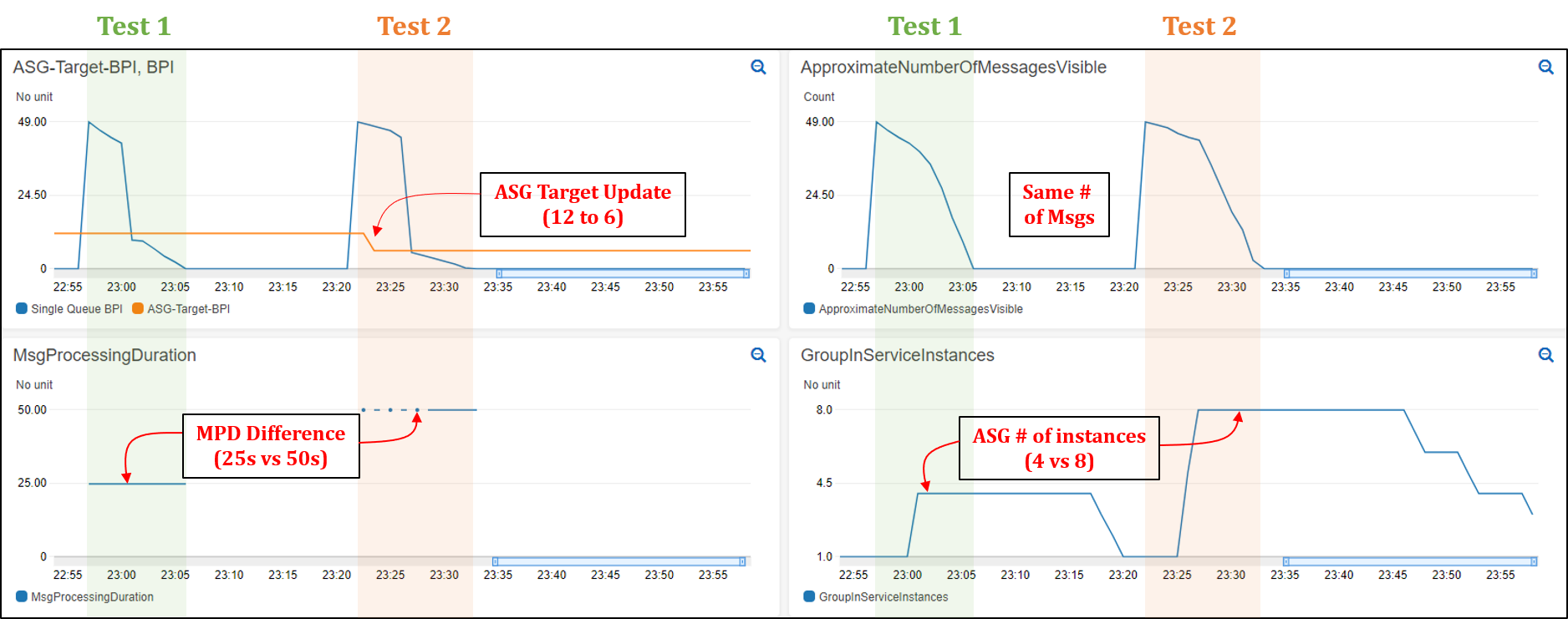


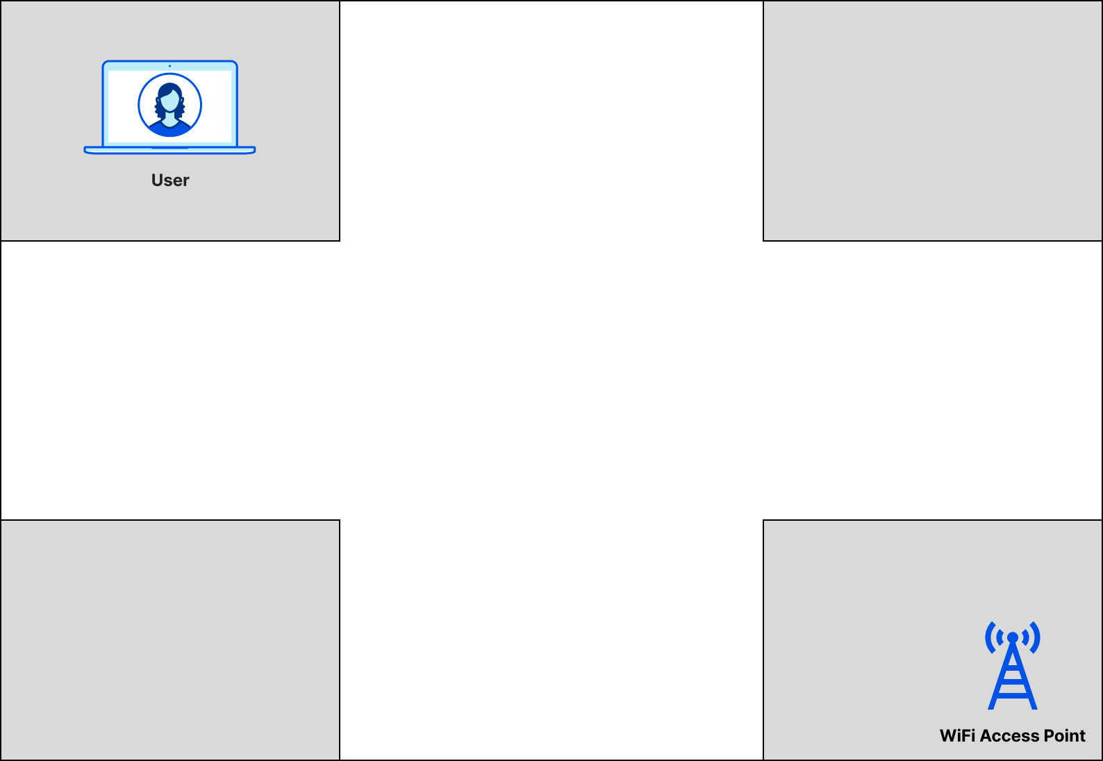
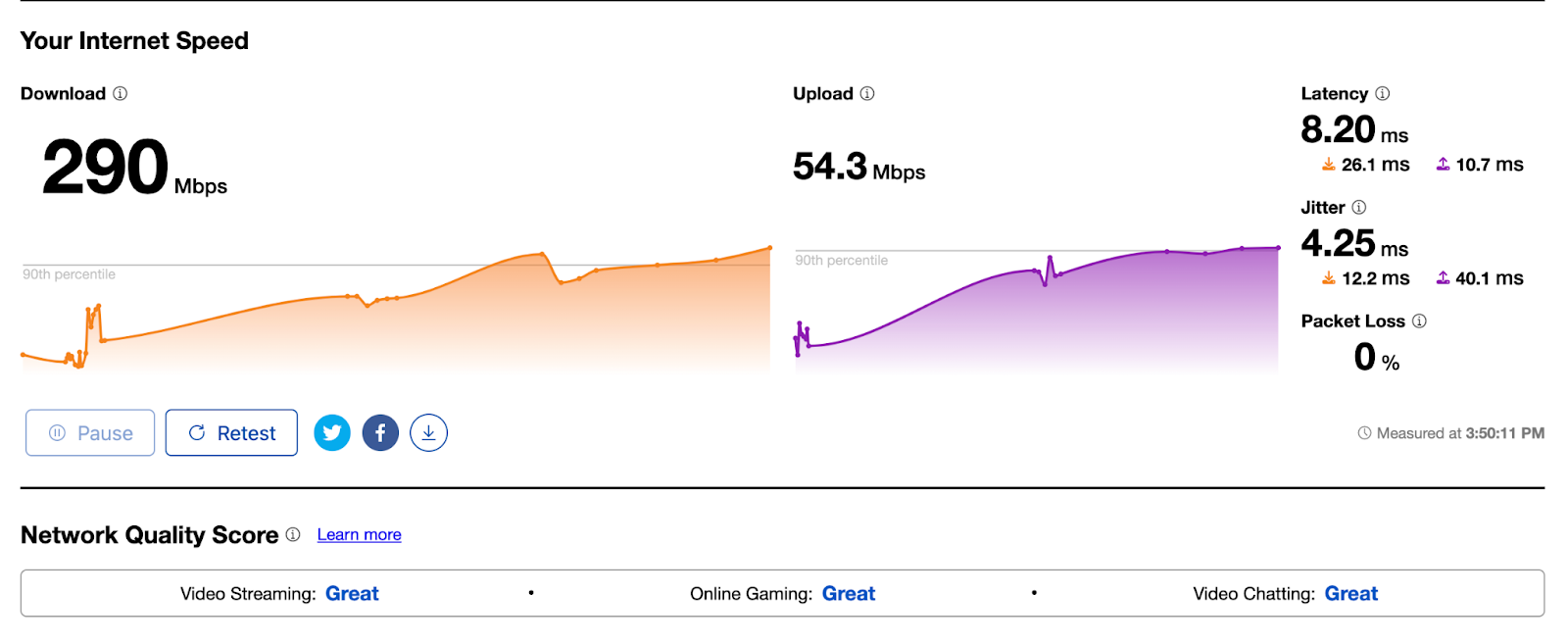
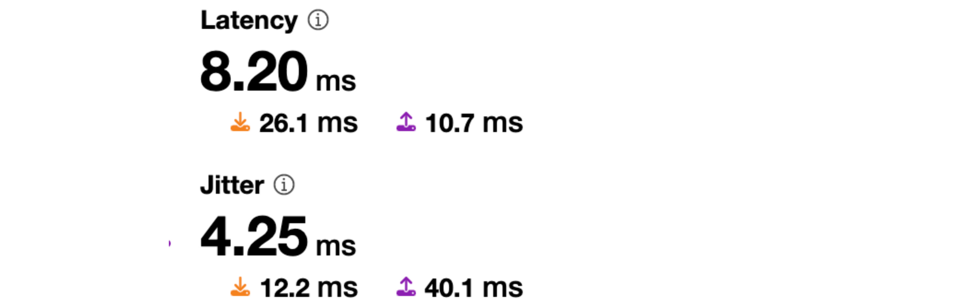
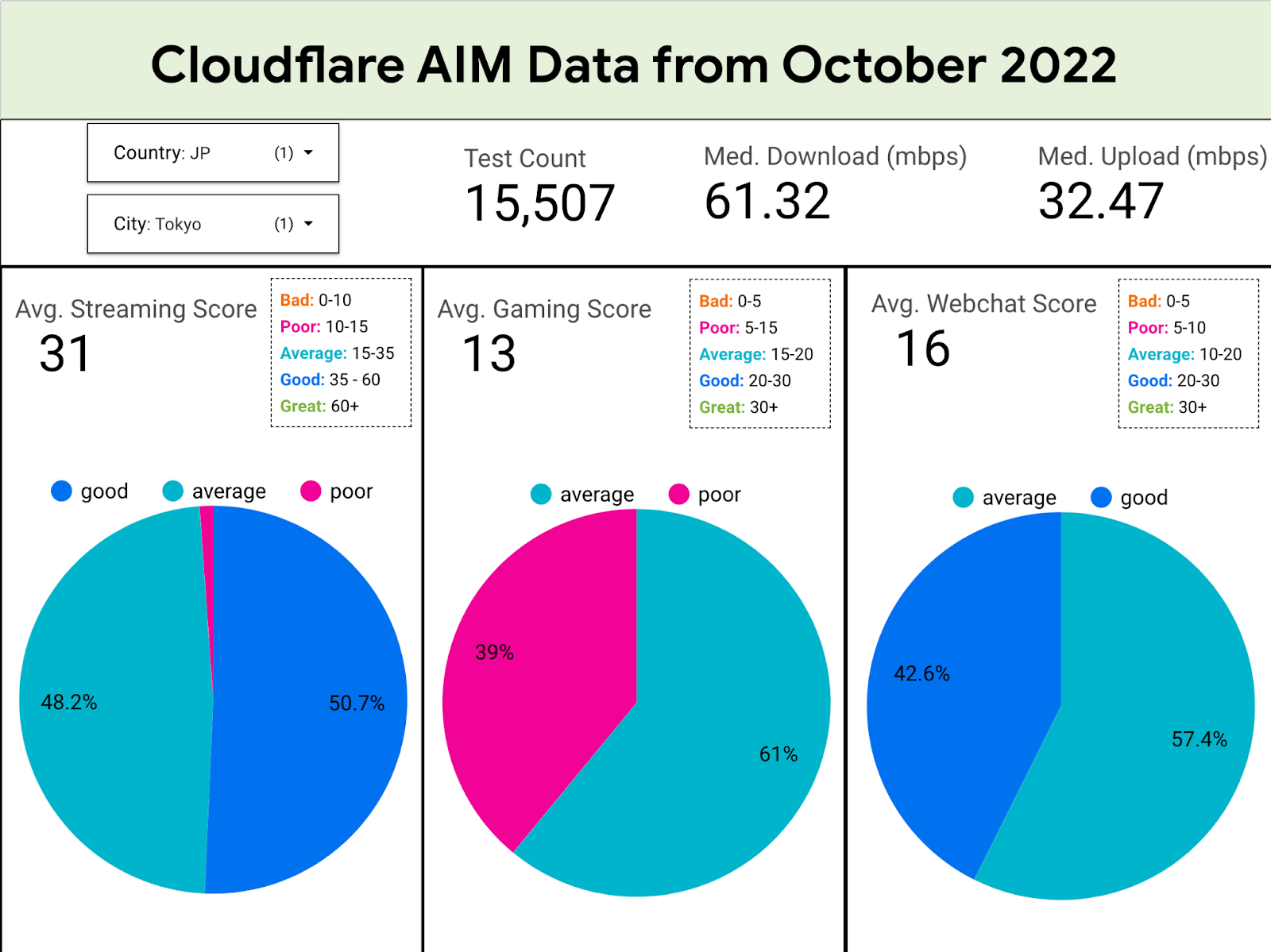


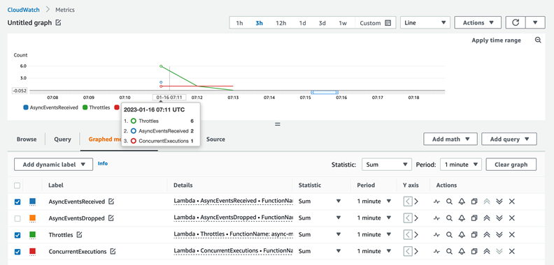


 Ramesh Ranganathan is a Senior Partner Solution Architect at AWS. He works with AWS customers and partners to provide guidance on enterprise cloud adoption, application modernization and cloud native development. He is passionate about technology and enjoys experimenting with AWS Serverless services.
 Kamen Sharlandjiev is an Analytics Specialist Solutions Architect and Amazon AppFlow expert. He’s on a mission to make life easier for customers who are facing complex data integration challenges. His secret weapon? Fully managed, low-code AWS services that can get the job done with minimal effort and no coding.
 Amit Shah is a cloud based modern data architecture expert and currently leading AWS Data Analytics practice in Atos. Based in Pune in India, he has 20+ years of experience in data strategy, architecture, design and development. He is on a mission to help organization become data-driven.