Security updates for Thursday

Post Syndicated from jake original https://lwn.net/Articles/960436/

Security updates have been issued by Debian (debian-security-support, firefox-esr, openjdk-11, and python-asyncssh), Fedora (glibc, python-templated-dictionary, thunderbird, and xorg-x11-server-Xwayland), Gentoo (Chromium, Google Chrome, Microsoft Edge and WebKitGTK+), Red Hat (firefox, gnutls, libssh, thunderbird, and tigervnc), SUSE (mbedtls, rear116, rear1172a, runc, squid, and tinyssh), and Ubuntu (glibc and runc).

Facebook’s Extensive Surveillance Network

Post Syndicated from Bruce Schneier original https://www.schneier.com/blog/archives/2024/02/facebooks-extensive-surveillance-network.html

Consumer Reports is reporting that Facebook has built a massive surveillance network:

Using a panel of 709 volunteers who shared archives of their Facebook data, Consumer Reports found that a total of 186,892 companies sent data about them to the social network. On average, each participant in the study had their data sent to Facebook by 2,230 companies. That number varied significantly, with some panelists’ data listing over 7,000 companies providing their data. The Markup helped Consumer Reports recruit participants for the study. Participants downloaded an archive of the previous three years of their data from their Facebook settings, then provided it to Consumer Reports.

This isn’t data about your use of Facebook. This data about your interactions with other companies, all of which is correlated and analyzed by Facebook. It constantly amazes me that we willingly allow these monopoly companies that kind of surveillance power.

Here’s the Consumer Reports study. It includes policy recommendations:

Many consumers will rightly be concerned about the extent to which their activity is tracked by Facebook and other companies, and may want to take action to counteract consistent surveillance. Based on our analysis of the sample data, consumers need interventions that will:

  • Reduce the overall amount of tracking.
  • Improve the ability for consumers to take advantage of their right to opt out under state privacy laws.
  • Empower social media platform users and researchers to review who and what exactly is being advertised on Facebook.
  • Improve the transparency of Facebook’s existing tools.

And then the report gives specifics.

An integrated learning experience for young people

Post Syndicated from Joanne Vincent original https://www.raspberrypi.org/blog/code-editor-integration/

We’re currently trialling the full integration of our Code Editor in some of the projects on our Projects site, with the aim of providing a seamless experience for young learners. Our Projects site provides hundreds of free coding projects with step-by-step instructions for young people to use at school, in Code Clubs and CoderDojo clubs, and at home. When learners make text-based programming projects in our Python and web design project paths, they use our Code Editor to write and run code in a web browser.

A young person at a computer in a classroom.

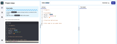
Our new integrated learning experience allows young people to follow the project instructions and work in the Code Editor in a single window. By providing a simpler workspace, where learners do not need to switch between windows to read instructions and input code, we aim to reduce cognitive load and make it easier for young people to learn.

How the new integrated experience works

In the integrated project workspace, learners can access the project instructions, coding area, and output (where they can see what they have made) all in the same view. We have reorganised the project guides into short, easy-to-follow steps made up of simple instructions, including code snippets and modelled examples, for learners to work through to create their projects. The project guides feature fresh designs for different types of learning content, such as instruction steps, concept steps, code snippets, tips, and debugging help.

A screenshot of the new Code Editor.

We have also optimised this learning experience for young people using mobiles and tablets. On mobile devices, a new ‘Steps’ tab appears alongside the ‘Code’ and ‘Output’ tabs, enabling learners to easily navigate to the project guide and follow the steps to make their projects.

Try out our new learning experience

We are testing our new integrated learning experience as a beta version in three projects: 

  • Hello world (part of our ‘Introduction to Python’ project path) 
  • Target practice (part of our ‘Introduction to Python’ project path) 
  • Anime expressions (part of our ‘Introduction to web development’ project path) 

In each of these projects, young people can choose to complete the original version of the project, with the project instructions and Code Editor in separate windows, or click the button on the project page to try out the new integrated learning experience.

A screenshot of the new Code Editor.

We’d love to hear how your young learners get on with this new integrated experience. Try it out in the three projects above and share your feedback with us here.

Code Editor developments have been made possible with generous support from the Cisco Foundation.

The post An integrated learning experience for young people appeared first on Raspberry Pi Foundation.

Introducing zabbix_utils – the official Python library for Zabbix API

Post Syndicated from Aleksandr Iantsen original https://blog.zabbix.com/python-zabbix-utils/27056/

Zabbix is a flexible and universal monitoring solution that integrates with a wide variety of different systems right out of the box. Despite actively expanding the list of natively supported systems for integration (via templates or webhook integrations), there may still be a need to integrate with custom systems and services that are not yet supported. In such cases, a library taking care of implementing interaction protocols with the Zabbix API, Zabbix server/proxy, or Agent/Agent2 becomes extremely useful. Given that Python is widely adopted among DevOps and SRE engineers as well as server administrators, we decided to release a library for this programming language first.

We are pleased to introduce zabbix_utils – a Python library for seamless interaction with Zabbix API, Zabbix server/proxy, and Zabbix Agent/Agent2. Of course, there are popular community solutions for working with these Zabbix components in Python. Keeping this fact in mind, we have tried to consolidate popular issues and cases along with our experience to develop as convenient a tool as possible. Furthermore, we made sure that transitioning to the tool is as straightforward and clear as possible. Thanks to official support, you can be confident that the current version of the library is compatible with the latest Zabbix release.

In this article, we will introduce you to the main capabilities of the library and provide examples of how to use it with Zabbix components.

Usage Scenarios

The zabbix_utils library can be used in the following scenarios, but is not limited to them:

  • Zabbix automation
  • Integration with third-party systems
  • Custom monitoring solutions
  • Data export (hosts, templates, problems, etc.)
  • Integration into your Python application for Zabbix monitoring support
  • Anything else that comes to mind

You can use zabbix_utils for automating Zabbix tasks, such as scripting the automatic monitoring setup of your IT infrastructure objects. This can involve using ZabbixAPI for the direct management of Zabbix objects, Sender for sending values to hosts, and Getter for gathering data from Agents. We will discuss Sender and Getter in more detail later in this article.

For example, let’s imagine you have an infrastructure consisting of different branches. Each server or workstation is deployed from an image with an automatically configured Zabbix Agent and each branch is monitored by a Zabbix proxy since it has an isolated network. Your custom service or script can fetch a list of this equipment from your CMDB system, along with any additional information. It can then use this data to create hosts in Zabbix and link the necessary templates using ZabbixAPI based on the received information. If the information from CMDB is insufficient, you can request data directly from the configured Zabbix Agent using Getter and then use this information for further configuration and decision-making during setup. Another part of your script can access AD to get a list of branch users to update the list of users in Zabbix through the API and assign them the appropriate permissions and roles based on information from AD or CMDB (e.g., editing rights for server owners).

Another use case of the library may be when you regularly export templates from Zabbix for subsequent import into a version control system. You can also establish a mechanism for loading changes and rolling back to previous versions of templates. Here a variety of other use cases can also be implemented – it’s all up to your requirements and the creative usage of the library.

Of course, if you are a developer and there is a requirement to implement Zabbix monitoring support for your custom system or tool, you can implement sending data describing any events generated by your custom system/tool to Zabbix using Sender.

Installation and Configuration

To begin with, you need to install the zabbix_utils library. You can do this in two main ways:

  • By using pip:
~$ pip install zabbix_utils
  • By cloning from GitHub:
~$ git clone https://github.com/zabbix/python-zabbix-utils
~$ cd python-zabbix-utils/
~$ python setup.py install

No additional configuration is required. But you can specify values for the following environment variables: ZABBIX_URL, ZABBIX_TOKEN, ZABBIX_USER, ZABBIX_PASSWORD if you need. These use cases are described in more detail below.

Working with Zabbix API

To work with Zabbix API, it is necessary to import the ZabbixAPI class from the zabbix_utils library:

from zabbix_utils import ZabbixAPI

If you are using one of the existing popular community libraries, in most cases, it will be sufficient to simply replace the ZabbixAPI import statement with an import from our library.

At that point you need to create an instance of the ZabbixAPI class. T4here are several usage scenarios:

  • Use preset values of environment variables, i.e., not pass any parameters to ZabbixAPI:
~$ export ZABBIX_URL="https://zabbix.example.local"
~$ export ZABBIX_USER="Admin"
~$ export ZABBIX_PASSWORD="zabbix"
from zabbix_utils import ZabbixAPI


api = ZabbixAPI()
  • Pass only the Zabbix API address as input, which can be specified as either the server IP/FQDN address or DNS name (in this case, the HTTP protocol will be used) or as an URL, and the authentication data should still be specified as values for environment variables:
~$ export ZABBIX_USER="Admin"
~$ export ZABBIX_PASSWORD="zabbix"
from zabbix_utils import ZabbixAPI

api = ZabbixAPI(url="127.0.0.1")
  • Pass only the Zabbix API address to ZabbixAPI, as in the example above, and pass the authentication data later using the login() method:
from zabbix_utils import ZabbixAPI

api = ZabbixAPI(url="127.0.0.1")
api.login(user="Admin", password="zabbix")
  • Pass all parameters at once when creating an instance of ZabbixAPI; in this case, there is no need to subsequently call login():
from zabbix_utils import ZabbixAPI

api = ZabbixAPI(
    url="127.0.0.1",
    user="Admin",
    password="zabbix"
)

The ZabbixAPI class supports working with various Zabbix versions, automatically checking the API version during initialization. You can also work with the Zabbix API version as an object as follows:

from zabbix_utils import ZabbixAPI

api = ZabbixAPI()

# ZabbixAPI version field
ver = api.version
print(type(ver).__name__, ver) # APIVersion 6.0.24

# Method to get ZabbixAPI version
ver = api.api_version()
print(type(ver).__name__, ver) # APIVersion 6.0.24

# Additional methods
print(ver.major)    # 6.0
print(ver.minor)    # 24
print(ver.is_lts()) # True

As a result, you will get an APIVersion object that has major and minor fields returning the respective minor and major parts of the current version, as well as the is_lts() method, returning true if the current version is LTS (Long Term Support), and false otherwise. The APIVersion object can also be compared to a version represented as a string or a float number:

# Version comparison
print(ver < 6.4)      # True
print(ver != 6.0)     # False
print(ver != "6.0.5") # True

If the account and password (or starting from Zabbix 5.4 – token instead of login/password) are not set as environment variable values or during the initialization of ZabbixAPI, then it is necessary to call the login() method for authentication:

from zabbix_utils import ZabbixAPI

api = ZabbixAPI(url="127.0.0.1")
api.login(token="xxxxxxxx")

After authentication, you can make any API requests described for all supported versions in the Zabbix documentation.

The format for calling API methods looks like this:

api_instance.zabbix_object.method(parameters)

For example:

api.host.get()

After completing all the necessary API requests, it’s necessary to execute logout() if authentication was done using login and password:

api.logout()

More examples of usage can be found here.

Sending Values to Zabbix Server/Proxy

There is often a need to send values to Zabbix Trapper. For this purpose, the zabbix_sender utility is provided. However, if your service or script sending this data is written in Python, calling an external utility may not be very convenient. Therefore, we have developed the Sender, which will help you send values to Zabbix server or proxy one by one or in groups. To work with Sender, you need to import it as follows:

from zabbix_utils import Sender

After that, you can send a single value:

from zabbix_utils import Sender

sender = Sender(server='127.0.0.1', port=10051)
resp = sender.send_value('example_host', 'example.key', 50, 1702511920)

Alternatively, you can put them into a group for simultaneous sending, for which you need to additionally import ItemValue:

from zabbix_utils import ItemValue, Sender


items = [
    ItemValue('host1', 'item.key1', 10),
    ItemValue('host1', 'item.key2', 'Test value'),
    ItemValue('host2', 'item.key1', -1, 1702511920),
    ItemValue('host3', 'item.key1', '{"msg":"Test value"}'),
    ItemValue('host2', 'item.key1', 0, 1702511920, 100)
]

sender = Sender('127.0.0.1', 10051)
response = sender.send(items)

For cases when there is a necessity to send more values than Zabbix Trapper can accept at one time, there is an option for fragmented sending, i.e. sequential sending in separate fragments (chunks). By default, the chunk size is set to 250 values. In other words, when sending values in bulk, the 400 values passed to the send() method for sending will be sent in two stages. 250 values will be sent first, and the remaining 150 values will be sent after receiving a response. The chunk size can be changed, to do this, you simply need to specify your value for the chunk_size parameter when initializing Sender:

from zabbix_utils import ItemValue, Sender


items = [
    ItemValue('host1', 'item.key1', 10),
    ItemValue('host1', 'item.key2', 'Test value'),
    ItemValue('host2', 'item.key1', -1, 1702511920),
    ItemValue('host3', 'item.key1', '{"msg":"Test value"}'),
    ItemValue('host2', 'item.key1', 0, 1702511920, 100)
]

sender = Sender('127.0.0.1', 10051, chunk_size=2)
response = sender.send(items)

In the example above, the chunk size is set to 2. So, 5 values passed will be sent in three requests of two, two, and one value, respectively.

If your server has multiple network interfaces, and values need to be sent from a specific one, the Sender provides the option to specify a source_ip for the sent values:

from zabbix_utils import Sender

sender = Sender(
    server='zabbix.example.local',
    port=10051,
    source_ip='10.10.7.1'
)
resp = sender.send_value('example_host', 'example.key', 50, 1702511920)

It also supports reading connection parameters from the Zabbix Agent/Agent2 configuration file. To do this, set the use_config flag, after which it is not necessary to pass connection parameters when creating an instance of Sender:

from zabbix_utils import Sender

sender = Sender(
    use_config=True,
    config_path='/etc/zabbix/zabbix_agent2.conf'
)
response = sender.send_value('example_host', 'example.key', 50, 1702511920)

Since the Zabbix Agent/Agent2 configuration file can specify one or even several Zabbix clusters consisting of multiple Zabbix server instances, Sender will send data to the first available server of each cluster specified in the ServerActive parameter in the configuration file. In case the ServerActive parameter is not specified in the Zabbix Agent/Agent2 configuration file, the server address from the Server parameter with the standard Zabbix Trapper port – 10051 will be taken.

By default, Sender returns the aggregated result of sending across all clusters. But it is possible to get more detailed information about the results of sending for each chunk and each cluster:

print(response)
# {"processed": 2, "failed": 0, "total": 2, "time": "0.000108", "chunk": 2}

if response.failed == 0:
    print(f"Value sent successfully in {response.time}")
else:
    print(response.details)
    # {
    #     127.0.0.1:10051: [
    #         {
    #             "processed": 1,
    #             "failed": 0,
    #             "total": 1,
    #             "time": "0.000051",
    #             "chunk": 1
    #         }
    #     ],
    #     zabbix.example.local:10051: [
    #         {
    #             "processed": 1,
    #             "failed": 0,
    #             "total": 1,
    #             "time": "0.000057",
    #             "chunk": 1
    #         }
    #     ]
    # }
    for node, chunks in response.details.items():
        for resp in chunks:
            print(f"processed {resp.processed} of {resp.total} at {node.address}:{node.port}")
            # processed 1 of 1 at 127.0.0.1:10051
            # processed 1 of 1 at zabbix.example.local:10051

More usage examples can be found here.

Getting values from Zabbix Agent/Agent2 by item key.

Sometimes it can also be useful to directly retrieve values from the Zabbix Agent. To assist with this task, zabbix_utils provides the Getter. It performs the same function as the zabbix_get utility, allowing you to work natively within Python code. Getter is straightforward to use; just import it, create an instance by passing the Zabbix Agent’s address and port, and then call the get() method, providing the data item key for the value you want to retrieve:

from zabbix_utils import Getter

agent = Getter('10.8.54.32', 10050)
resp = agent.get('system.uname')

In cases where your server has multiple network interfaces, and requests need to be sent from a specific one, you can specify the source_ip for the Agent connection:

from zabbix_utils import Getter

agent = Getter(
    host='zabbix.example.local',
    port=10050,
    source_ip='10.10.7.1'
)
resp = agent.get('system.uname')

The response from the Zabbix Agent will be processed by the library and returned as an object of the AgentResponse class:

print(resp)
# {
#     "error": null,
#     "raw": "Linux zabbix_server 5.15.0-3.60.5.1.el9uek.x86_64",
#     "value": "Linux zabbix_server 5.15.0-3.60.5.1.el9uek.x86_64"
# }

print(resp.error)
# None

print(resp.value)
# Linux zabbix_server 5.15.0-3.60.5.1.el9uek.x86_64

More usage examples can be found here.

Conclusions

The zabbix_utils library for Python allows you to take full advantage of monitoring using Zabbix, without limiting yourself to the integrations available out of the box. It can be valuable for both DevOps and SRE engineers, as well as Python developers looking to implement monitoring support for their system using Zabbix.

In the next article, we will thoroughly explore integration with an external service using this library to demonstrate the capabilities of zabbix_utils more comprehensively.

Questions

Q: Which Agent versions are supported for Getter?

A: Supported versions of Zabbix Agents are the same as Zabbix API versions, as specified in the readme file. Our goal is to create a library with full support for all Zabbix components of the same version.

Q: Does Getter support Agent encryption?

A: Encryption support is not yet built into Sender and Getter, but you can create your wrapper using third-party libraries for both.

from zabbix_utils import Sender

def psk_wrapper(sock, tls):
    # ...
    # Implementation of TLS PSK wrapper for the socket
    # ...

sender = Sender(
    server='zabbix.example.local',
    port=10051,
    socket_wrapper=psk_wrapper
)

More examples can be found here.

Q: Is it possible to set a timeout value for Getter?

A: The response timeout value can be set for the Getter, as well as for ZabbixAPI and Sender. In all cases, the timeout is set for waiting for any responses to requests.

# Example of setting a timeout for Sender
sender = Sender(server='127.0.0.1', port=10051, timeout=30)

# Example of setting a timeout for Getter
agent = Getter(host='127.0.0.1', port=10050, timeout=30)

Q: Is parallel (asynchronous) mode supported?

A: Currently, the library does not include asynchronous classes and methods, but we plan to develop asynchronous versions of ZabbixAPI and Sender.

Q: Is it possible to specify multiple servers when sending through Sender without specifying a configuration file (for working with an HA cluster)?

A: Yes, it’s possible by the following way:

from zabbix_utils import Sender


zabbix_clusters = [
    [
        'zabbix.cluster1.node1',
        'zabbix.cluster1.node2:10051'
    ],
    [
        'zabbix.cluster2.node1:10051',
        'zabbix.cluster2.node2:20051',
        'zabbix.cluster2.node3'
    ]
]

sender = Sender(clusters=zabbix_clusters)
response = sender.send_value('example_host', 'example.key', 10, 1702511922)

print(response)
# {"processed": 2, "failed": 0, "total": 2, "time": "0.000103", "chunk": 2}

print(response.details)
# {
#     "zabbix.cluster1.node1:10051": [
#         {
#             "processed": 1,
#             "failed": 0,
#             "total": 1,
#             "time": "0.000050",
#             "chunk": 1
#         }
#     ],
#     "zabbix.cluster2.node2:20051": [
#         {
#             "processed": 1,
#             "failed": 0,
#             "total": 1,
#             "time": "0.000053",
#             "chunk": 1
#         }
#     ]
# }

The post Introducing zabbix_utils – the official Python library for Zabbix API appeared first on Zabbix Blog.

„Тоест“ на 6!

Post Syndicated from Тоест original https://www.toest.bg/toest-na-6/

„Тоест“ на 6!

Скъпи приятели на „Тоест“, станахме на 6 години!

„Станахме“, защото всички ние заедно – екип и читатели, правим медията „Тоест“. Този рожден ден е празник колкото за хората от екипа, толкова и за всички вас, които вече 6 години ни подкрепяте и абсолютно безкомпромисно ни доказвате, че една качествена медия може да се издържа благодарение на своята взискателна, активна и вярна публика. Благодарим ви от сърце, че сме заедно!

Черпим всички с шоколади на корем от „Гайо“, които може да поръчате тук. Пускаме духовата музика в сърцата и душите и вперваме поглед в хоризонта на седмата година, в която си пожелаваме отново да пристигнем заедно. За да се случи това, продължавайте да ни подкрепяте. Ето какви са начините: https://www.toest.bg/support/

Пращаме ви сърца и живи цветя и не смеем да си пожелаем нищо повече, защото най-важното за една медия вече го имаме – публика като вас! Честит „Тоест“!

Права на семейството или права на детето?

Post Syndicated from Светла Енчева original https://www.toest.bg/prava-na-semeystvoto-ili-prava-na-deteto/

Права на семейството или права на детето?

Чували сте да се говори за семейството, сякаш то е личност, която има права. Или по-скоро дете в риск, което има нужда от закрила. Да припомним например новогодишното изявление на президентите на Унгария, Сърбия и България, в което се казваше, че семействата „заслужават закрила, помощ и признание“. Разбира се, в името на децата. На правото на семействата да отглеждат децата си, както намерят за добре, се противопоставя безличната държавна машина, която отнема деца от родителите им. Но винаги ли родителите са най-доброто за едно дете?

Когато детето само̀ поиска закрила от държавата

Последният случай, разбунил духовете, е за момче на 13 или 14 години, което не желае да живее с родителите си. Причините за това са, че то няма достъп до образование (освен като частен ученик или в нелицензирани училища), нито до здравеопазване и иска да живее като другите деца. За случая се разчува от репортаж на БНТ и продължението му. При опита на родителите да изведат детето си от страната то е потърсило помощ от полицаите на летището, след което е пожелало да бъде настанено в център за социални услуги.

Министерството на труда и социалната политика излезе със становище по случая, на който дава гласност и Албена Тодорова – една от лелите на тийнейджъра. Тя разказва как той нееднократно е заявявал, че иска да има нормален дом в България, а не да живее в Бразилия, където няма постоянно жилище и където пребивава с родителите си, вярващи във всевъзможни конспиративни теории. При опит да бъде насила изведено от училището в България, в което е записано, момчето е ударено от приятел на майката и челюстта му е счупена. След това обаче майката продължавала да събира детето и този човек на едно място.

За „Тоест“ Тодорова уточни, че ученици от по-горен клас са се притекли на помощ на момчето, както и че то вече може да се храни самостоятелно, но няма как да бъде заведено на лекар, защото роднините, които се грижат за него, не са му попечители, нито настойници.

Майката на детето от своя страна обвинява роднините, че са го манипулирали. Тя отрича да го е удряла и твърди, че то няма нараняване, но не коментира информацията друг човек да е упражнил насилие върху него. Във Facebook майката публикува десетки снимки на момчето като доказателство колко щастливо и пълноценно е живяло то под грижите на родителите си. По този начин тя излага публично лични данни на дете против волята му.

Буда, който стана Атанас

Случаят с тийнейджъра, който не иска да живее с родителите си, даде повод за полярни реакции. Докато едни подкрепят желанието на неговите баби и лели да му осигурят нормална среда на живот, за други така се нарушава правото на родителите да отглеждат детето си според собствените си разбирания. За тях по дефиниция родителите имат право, а държавата е в ролята на лошата мащеха.

Подобни дискусии имаше и във връзка с друг случай – на майката, родила и отглеждаща детето си съвсем сама и в пълна изолация и наричаща го Буда. В продължение на три години тя дори е отказвала да го регистрира и то да получи ЕГН, за да не попадне в „дяволската система“. Детето е живяло без достъп до ток и течаща вода, да не говорим за здравеопазване. Но пък в компанията на много ножове. Първото бебе на майката е починало по време на домашно раждане.

И при този казус част от общественото мнение застана на страната на майката и на правото ѝ да отглежда своето дете в съответствие със собствените си ценности. Не само въпреки законите, а и въпреки рисковете за здравето, живота и развитието на момченцето. Решението детето да бъде настанено в приемно семейство, а майката – в център за психично здраве, стана обект на остри критики.

Няколко месеца по-късно детето е върнато на майка си и те живеят при свой познат. То вече има ЕГН и е регистрирано с името Атанас, а жената продължава да получава подкрепа от социалните служби, включително и за психичното си заболяване, което е установено.

Помните ли неприетата Стратегия за детето?

Защитата на родителите в случаи като тези, за които стана дума, е в духа на кампанията срещу Стратегията за детето през 2019 г., довела до неприемането ѝ. Тя се разгърна по начин, подобен на кампанията срещу Истанбулската конвенция. А и двигателите ѝ бяха, общо взето, същите, като започнем от Александър Урумов – тогавашния пиар на Военното министерство, политик от ВМРО, евангелски проповедник и агент на ДС. Лайтмотивът беше, че ако Стратегията се приеме, държавата ще отнема деца от родителите им „заради едно шамарче“.

Кампанията сериозно затрудни дейността на организациите, работещи в сферата на закрилата на децата, като някои от тях станаха обект и на заплахи. Тя продължи дълго време след като Стратегията не беше приета. В края на 2020 г. например ВМРО внесоха проект за промяна в Закона за закрила на детето с аргумента, че „детето не е отделен субект и това трябва ясно да залегне във всички нормативни актове, които касаят материята“.

Докато България продължава да няма стратегически документ за децата, през 2022 г. беше приета европейска Стратегия за правата на детето (2022–2027). Сред най-важните ѝ цели са свобода от насилие за всички деца и даване на глас на всяко дете. В нея детето се разглежда като личност с права, а не като обект, подвластен на родителите си или на държавата.

И щипка расизъм

Впрочем наблюдава се една интересна особеност в нагласите към правата на родителите, децата и ролята на държавата в регулирането им. Когато се предпоставя абсолютното право на родителите да определят кое е най-доброто за децата им, се имат предвид основно семейства на етнически българи. Що се отнася до ромските родители, общественото мнение застава на страната на държавата и законите.

Така например много критики и подигравки отнесоха родителите от ромските махали в няколко града, които в края на 2019 г. едновременно изпаднаха в паника, че социалните ще им вземат децата, и нахлуха в училищата да си ги приберат. Тогава тези родители бяха квалифицирани в социалните групи с епитети като „първобитни“. Такива епитети нямаше за родителите – етнически българи, страхуващи се, че зли норвежци могат да им откраднат децата.

По-сериозният проблем е, че за истерията в ромските махали не беше потърсена отговорност от онези, които размахваха Стратегията за детето като плашило, като започнем от Александър Урумов. В кампанията срещу Стратегията (както и срещу Истанбулската конвенция) бяха много гласовити някои евангелски църкви. Ромски родители, уплашени, че държавата ще им вземе децата, твърдяха, че са чули това от пастора на църквата в махалата.

Може ли семейната „клетка“ да бъде злокачествена?

Метафората за семейството като основна клетка на обществото е неоснователна, защото обществото не се състои от семейства. Затова пък е популярна. Организмите са изградени от клетки, но има и клетки, които „решават“ да се развиват „на своя глава“. Те започват да се размножават безконтролно, като по този начин вредят на организма и могат дори да го убият.

Обществото има механизми, благодарение на които се удържа като едно цяло. Сред най-важните от тях е образованието. Една от целите на публичното образование е да социализира децата, тоест да ги възпита в основните ценности и норми на дадено общество. Училището съвсем не е „безгрешно“, то има достатъчно „трески за дялане“. Но то е такова, каквото е и самото общество. 

Ситуацията с публичното здравеопазване е подобна, доколкото не на последно място то би следвало да включва превенция на социално значими заболявания. Последствията от решенията на много семейства да не се доверяват на здравната система са очевидни. Отказът от ваксиниране на децата например води до връщане на заболявания като морбили и полиомиелит, които почти са изкоренени благодарение на масовите имунизации.

Ето защо, ако възприемаме семейството като клетка, добре е да имаме предвид, че тя може да бъде и туморна. Зачитането на правата на децата е важно преди всичко за самите деца, но далеч не само за тях. Няма как да се изгради читаво общество от хора, чиито собствени права не са били уважавани и които са научени, че всичко извън семейството е зло.

Gigabyte R183-Z95 Review Dual AMD EPYC Server with a EDSFF Twist

Post Syndicated from Patrick Kennedy original https://www.servethehome.com/gigabyte-r183-z95-review-dual-amd-epyc-server-with-a-edsff-twist-kioxia/

The Gigabyte R183-Z95 is a 1U server with 17x NVMe SSD slots standard, along with dual AMD EPYC 9004 processors for a very cool system

The post Gigabyte R183-Z95 Review Dual AMD EPYC Server with a EDSFF Twist appeared first on ServeTheHome.

Managing dynamic marketplace content at scale: Grab’s approach to content moderation

Post Syndicated from Grab Tech original https://engineering.grab.com/dynamic-marketplace

In the fast-paced world of on-demand delivery, maintaining safe marketplaces is a complex undertaking. Grab, a leading superapp in Southeast Asia, operates GrabFood and GrabMart, two popular marketplaces that connect consumers with a wide range of food and daily necessities. With more than 100k listings for different items updated daily by our merchants across eight different countries, Grab is rising to the challenge of ensuring that its marketplaces remain compliant with its own policies, government regulations as well as platform policies.

This article provides an overview of how Grab employs a combination of automated and manual content moderation to manage its dynamic marketplace content efficiently, while also collaborating with Google to ensure marketplace safety. Stay tuned for future articles that will delve deeper into the technology and solutions used for content moderation.

Dynamic Marketplace Landscape

Marketplaces like GrabFood and GrabMart are at the forefront of connecting merchants and consumers. These marketplaces provide an avenue for merchants to showcase their offerings, enabling consumers to conveniently access a plethora of on-demand options. However, in an environment characterized by rapid changes as well as evolving regulatory frameworks, maintaining the integrity of these marketplaces becomes a formidable task.

Scale and Flexibility: A Dual Challenge

The cornerstone of Grab’s success lies in its ability to adapt to the unique regulations and requirements of each country it operates in. This necessitates a nuanced and multifaceted approach to content moderation. To achieve both scale and flexibility, Grab employs a proactive strategy that combines and leverages automated and manual moderation processes.

Automated Moderation

Automated moderation plays a pivotal role in efficiently managing the high volume of listings that undergo daily updates. Grab utilises advanced algorithms and machine learning technologies, built in-house, to scan listings everyday for potential violations of its own policies, government regulations and platform policies. This automation not only speeds up the process to put eligible listings on the Grab platform, but also ensures consistent adherence to predefined guidelines. However, automated moderation is not without its limitations, as contextual understanding and subjective judgment often require human intervention.

Manual Moderation

Recognising the nuanced nature of content moderation, Grab employs a team of human moderators who possess the cultural awareness and contextual understanding necessary to assess complex cases. These moderators review listings flagged by algorithms and machine learning technologies that require human judgment, ensuring that content aligns with Grab’s policies, local regulations as well as platform policies. Manual moderation adds a layer of human insight that automated systems may lack, contributing to a more accurate and contextually sensitive approach.

In its commitment to ensuring marketplace safety, Grab has also established a strong collaboration with Google. Grab works hand in hand with Google to collectively ensure adherence to Play Store policies and guidelines.

Grab

  • Programme Management: Poonam Gambhire, Shuyang Sun
  • Product: Chris Collard
  • Engineering: Shuya Ding, Kirubakaran Duraisamy, Xu Chen

Google

  • Play Policy: Siddhartha Paul Tiwari
  • Business Development: Mika Igarashi

Join us

Grab is the leading superapp platform in Southeast Asia, providing everyday services that matter to consumers. More than just a ride-hailing and food delivery app, Grab offers a wide range of on-demand services in the region, including mobility, food, package and grocery delivery services, mobile payments, and financial services across 428 cities in eight countries.

Powered by technology and driven by heart, our mission is to drive Southeast Asia forward by creating economic empowerment for everyone. If this mission speaks to you, join our team today!

A new and improved AWS CDK construct for Amazon DynamoDB tables

Post Syndicated from Anirudh Sharma original https://aws.amazon.com/blogs/devops/a-new-and-improved-aws-cdk-construct-for-amazon-dynamodb-tables/

Recently, we launched a new AWS Cloud Development Kit (CDK) construct for Amazon DynamoDB tables, known as TableV2. This construct provides a number of new features in addition to what the original construct offered, enabling CDK authors to create global tables, simplifying the configuration of global secondary indexes and auto scaling, as well as supporting AWS CloudFormation drift detection and import operations. We believe that this new construct will make it easier for organizations to build and manage their DynamoDB tables at scale, in addition to providing more flexibility and control over the configuration of tables.

AWS CDK is a framework for defining cloud infrastructure in code and provisioning it through AWS CloudFormation. Developers can use any of the supported programming languages to define reusable cloud components known as Constructs. A construct is a reusable and programmable component that represents AWS resources. CDK translates the high-level constructs defined by you into equivalent AWS CloudFormation templates. CloudFormation provisions the resources specified in the template, streamlining the usage of Infrastructure as a Code (IaC) on AWS.

In this post we’ll explore:

  • The reasoning behind the creation of a new L2 construct for DynamoDB tables.
  • Features of new L2 constructs along with examples.
  • The benefits of leveraging this new construct in terms of scalability, flexibility, and simplicity.

By understanding the reasons behind its development and exploring its capabilities through practical examples, you will gain a comprehensive understanding of how this new L2 construct can enhance their DynamoDB experience. Let’s dive in.

Background

The original DynamoDB L2 Table construct is a powerful and versatile tool for creating and managing DynamoDB tables. It allows you to easily define the schema of your table, as well as the provisioned throughput and replicas. It also supports features like global tables, secondary indexes, and streams.

However, the Table construct uses a custom resource to add replicas to the primary table. This means that a separate Lambda function is created as the resource provider in addition to the Table resources (primary table and any replicas). This can be cumbersome to manage and can lead to drift detection issues.

The new TableV2 construct is an abstraction built on top of the GlobalTable L1 construct. It uses the CloudFormation resource AWS::DynamoDB::GlobalTable to create and manage DynamoDB tables. This has two important benefits:

  1. CloudFormation is in control and aware of all replicas that make up the Global Table, which means you will experience drift detection across all the replicas. With the original table construct, CloudFormation was not aware of any replicas since this was being handled through the Lambda function being used as a resource provider.
  2. No extra resource (Lambda function) is created when replicas are configured with TableV2. This eliminates the need to manage an extra resource and the risk of troubleshooting issues that may arise with the custom resource. TableV2 simplifies the setup and maintenance of DynamoDB tables by using native CloudFormation constructs to directly manage replicas, without the need for a Lambda function. This results in a more efficient and streamlined experience for users.

The new TableV2 construct provides more fine-grained control to customers over the replicas created as part of the Global Table. Specifically, customers can specify properties like contributor insights, deletion protection, point-in-time recovery, table class, read capacity, and global secondary index options on a per-replica basis.

This means that customers can tailor their table setup to meet their specific needs and optimize their overall experience with the Global Table feature. For example, a customer might want to enable contributor insights for all replicas, but only enable deletion protection for the primary replica. Or, a customer might want to use a different table class for each replica, depending on the expected workload.

The new TableV2 construct also offers greater flexibility and customization options by allowing customers to specify these properties on a per-replica basis. This can be helpful for customers who need to have different configurations for their replicas, or who want to fine-tune the performance and availability of their tables.

In the next section, we will explore each of these properties in more detail and how they can be specified in the new construct.

Features Walk-through

The new TableV2 construct is the recommended CDK DynamoDB construct for creating both single tables and global tables. In this section, we will review some specific aspects of the TableV2 construct and how they can be implemented. The walkthrough will cover features like Replicas, Billing, and Encryption, providing a comprehensive understanding of its capabilities.

Replicas

One of the most important benefits of the new L2 construct is the ability to configure properties on a per-replica basis. For example, the following code creates a global DynamoDB table with contributor insights and point-in-time recovery enabled for the table:

import * as cdk from 'aws-cdk-lib';
import * as dynamodb from 'aws-cdk-lib/aws-dynamodb';

const app = new cdk.App();
const stack = new cdk.Stack(app, 'Stack', { env: { region: 'us-west-2' } });

const globalTable = new dynamodb.TableV2(stack, 'GlobalTable', {
  partitionKey: { name: 'pk', type: dynamodb.AttributeType.STRING },
  contributorInsights: true,
  pointInTimeRecovery: true,
  replicas: [
    {
      region: 'us-east-1',
      tableClass: dynamodb.TableClass.STANDARD_INFREQUENT_ACCESS,
      pointInTimeRecovery: false,
    },
    {
      region: 'us-east-2',
      contributorInsights: false,
    },
  ],
});

// This is an ITableV2 instance for the replica table in us-east-1
const replica = globalTable.replica('us-east-1');

This code creates two replicas, one in the us-east-1 region and one in the us-east-2 region. For the replica in the us-east-1 region, we disable point-in-time recovery and set the table class to STANDARD_INFREQUENT_ACCESS. For the replica in the us-east-2 region, we disable contributor insights. The TableV2 construct also enables users to work with individual instances of the replicas in a global table via the replica() method. We see how this can be utilized from the above code where an ITableV2 instance representing the replica in us-east-1 is returned.

This is particularly useful for the grant() and metric() methods. For example, the following code gives a user write access to a replica in us-east-1 region:

import { Construct } from 'constructs';
import { App, Stack, StackProps } from 'aws-cdk-lib';
import { ITableV2, TableV2 } from 'aws-cdk-lib/aws-dynamodb';
import { AttributeType } from 'aws-cdk-lib/aws-dynamodb';
import * as iam from 'aws-cdk-lib/aws-iam';


class FooStack extends Stack {
  public readonly globalTable: TableV2;

  public constructor(scope: Construct, id: string, props: StackProps) {
    super(scope, id, props);

    this.globalTable = new TableV2(this, 'GlobalTable', {
      partitionKey: { name: 'pk', type: AttributeType.STRING },
      replicas: [
        { region: 'us-east-1' },
        { region: 'us-east-2' },
      ],
    });
  }
}

interface BarStackProps extends StackProps {
  readonly replicaTable: ITableV2;
}

class BarStack extends Stack {
  public constructor(scope: Construct, id: string, props: BarStackProps) {
    super(scope, id, props);
    const user = new iam.User(this, 'User')

    // user is given grantWriteData permissions to replica in us-east-1
    props.replicaTable.grantWriteData(user);
  }
}

const app = new App();

const fooStack = new FooStack(app, 'FooStack', { env: { region: 'us-west-2', account: process.env.CDK_DEFAULT_ACCOUNT } });
const barStack = new BarStack(app, 'BarStack', {
  replicaTable: fooStack.globalTable.replica('us-east-1'),
  env: { region: 'us-east-1', account: process.env.CDK_DEFAULT_ACCOUNT },
});

Before the replica() method was introduced, grant methods on the original Table construct applied to the primary table and all replicas. This was because there was no way to pull out a specific replica. This limited a user’s ability to grant a specific principal read, write, or read/write permission to a specific replica. The replica() method enables granting specific permissions to individual replicas in a global table. It maintains consistent behavior across all methods in the ITableV2 interface, including grants and metrics.

Billing

Table billing is easily configured using the onDemand() or provisioned() static methods of the Billing class. If provisioned billing is configured, the user must provide read and write capacity, which can be easily configured using the fixed() or autoscaled() static methods of the Capacity class.

For example, to configure on-demand billing:

import * as cdk from 'aws-cdk-lib';
import { AttributeType, Billing, TableClass, TableV2 } from 'aws-cdk-lib/aws-dynamodb';
import { Construct } from 'constructs';


export class DynamodbStack extends cdk.Stack {
  constructor(scope: Construct, id: string, props?: cdk.StackProps) {
    super(scope, id, props);
    new TableV2(this, 'DynamoDBTable', {
      partitionKey: { name: 'id', type: AttributeType.STRING},
      replicas: [
        {region: 'us-east-2'},
        {region: 'us-west-1'}
      ],
      billing: Billing.onDemand(),
      tableClass: TableClass.STANDARD
    })
  }
}

To configure provisioned billing:

import * as cdk from 'aws-cdk-lib';
import { AttributeType, Billing, Capacity, TableClass, TableV2 } from 'aws-cdk-lib/aws-dynamodb';
import { Construct } from 'constructs';

export class DynamodbStack extends cdk.Stack {
  constructor(scope: Construct, id: string, props?: cdk.StackProps) {
    super(scope, id, props);
    new TableV2(this, 'DynamoDBTable', {
      partitionKey: { name: 'id', type: AttributeType.STRING},
      replicas: [
        {region: 'us-east-2'},
        {region: 'us-west-1'}
      ],
      billing: Billing.provisioned({
        readCapacity: Capacity.fixed(5),
        writeCapacity: Capacity.autoscaled({maxCapacity: 10})
      }),
      tableClass: TableClass.STANDARD
    })
  }
}

Note that with the previous Table construct, users had to set a billingMode property and configure readCapacity and writeCapacity as separate properties. Additionally, configuring autoscaled capacity required calling the autoScaleReadCapacity() or autoScaleWriteCapacity() method on an instance of the Table construct. Lastly, since readCapacity, writeCapacity, and billingMode were all individual properties, a user had to know not to provision read and write capacity for a table with PAY_PER_REQUEST billing mode. With the new Billing class, the user is guided into providing necessary properties via the onDemand() and provisioned() static methods.

Encryption

The TableEncryptionV2 class allows you to provide your own KMS keys for each replica instead of using the default AWS owned keys, thus encrypting every replica with a custom KMS key. This provides more granular control over the encryption of your DynamoDB tables.

Here is an example of how to use the TableEncryptionV2 class to encrypt each replica of a global table with a custom KMS key:

import * as cdk from 'aws-cdk-lib';
import { AttributeType, Billing, BillingMode, Capacity, TableBaseV2, TableEncryptionV2, TableV2 } from 'aws-cdk-lib/aws-dynamodb';
import { IKey, Key } from 'aws-cdk-lib/aws-kms';
import { Construct } from 'constructs';

interface KMSkeys extends cdk.StackProps {
  kmsuswest1: IKey;
  kmsuseast2: IKey;
}

export class GlobalTableStack extends cdk.Stack {
  //public readonly globalTable: TableV2;
  constructor(scope: Construct, id: string, props: KMSkeys) {
    super(scope, id, props);

    const replicaTableKeys = {
      "us-west-1": props.kmsuswest1.keyArn,
      "us-east-2": props.kmsuseast2.keyArn
    }
    const TableKMSKey=new Key(this, 'TableKMSKey', {
      alias: 'KMSuswest2Stack',
    }
    )

    new TableV2(this, 'GlobalTable', {
    tableName: 'FooTableFour',
    encryption: TableEncryptionV2.customerManagedKey(TableKMSKey,replicaTableKeys),

    partitionKey: {
    name: 'FooHashKey',
    type: AttributeType.STRING,
    },
    replicas: [
    {
      region: 'us-west-1',  
    },
    {
      region: 'us-east-2',
    },
  ],
    })
  }
}

The ability to provide custom KMS keys for each replica can help to improve the security of your DynamoDB tables. It also gives you more control over the encryption of your data. This can help you to meet specific compliance requirements.

Conclusion

In this post, I introduced the new AWS CDK TableV2 construct, highlighting its advantages over the original construct. Notably, TableV2 enables drift detection for replica tables and eliminates the need for an extra Lambda function custom resource. I delved into practical implementations, focusing on three key aspects: Replicas, Billing, and Encryption.

To summarize, TableV2 marks a substantial improvement over the original construct. Its user experience provides significant improvement over the original construct in several ways, such as:

  • Direct support for global tables: TableV2 makes it easy to create and manage global DynamoDB tables.
  • Easier configuration of global secondary indexes and Autoscaling: TableV2 provides a simplified and streamlined process for configuring global secondary indexes and Autoscaling.
  • More granular control over replicas: TableV2 allows you to configure properties on a per-replica basis, giving you more control over the performance and availability of your tables.
  • Improved API design and user experience: TableV2 improves the API design and user experience by implementing new classes for billing, capacity, and encryption.

Overall, TableV2 is a powerful and flexible construct that makes it easier to build and manage DynamoDB tables at scale. It is the preferred CDK DynamoDB construct for creating both single tables and global tables. If you are looking for a powerful and flexible way to build and manage DynamoDB tables, TableV2 is the perfect choice for you.

If you’re new to CDK and eager to get started, we highly recommend checking out the CDK documentation and the CDK workshop.

Anirudh Sharma

Anirudh is a Cloud Support Engineer 2 with an extensive background in DevOps offerings at AWS, and he is also a Subject Matter Expert in AWS ElasticBeanstalk and AWS CodeDeploy services. He loves helping customers and learning new services and technologies. He also loves travelling and has a goal to visit Japan someday. He is a Golden State Warriors fan and loves spending time with his family.

Announcing Generative AI CDK Constructs

Post Syndicated from Michael Tran original https://aws.amazon.com/blogs/devops/announcing-generative-ai-cdk-constructs/

Announced by Werner Vogels in his 2023 re:Invent Keynote, Generative AI CDK Constructs, an open-source extension of the AWS Cloud Development Kit (AWS CDK), provides well-architected multi-service patterns to quickly and efficiently create repeatable infrastructure required for generative AI projects on AWS. Our initial release includes five CDK constructs enabling key generative AI capabilities like question and answering, summarization, data ingestion for Retrieval Augmented Generation (RAG), and model deployment capabilities.

Simplify and Accelerate the Development of Applications with Generative AI

Developing generative AI applications is particularly challenging due to the rapidly evolving nature of the underlying technologies. As a result, developers are faced with the challenge of keeping up with changing paradigms and best practices. This often leads to varied and disjointed patterns as developers try crafting their own solutions from scratch. For instance, there are already hundreds of implementations of patterns like retrieval augmented generation(RAG), summarization, or chatbots.

AWS introduced the Cloud Development Kit (CDK), an open-source software development framework to define cloud infrastructure in code and provision it through AWS CloudFormation. CDK empowers developers to use high-level construct libraries that encapsulate AWS best practices, allowing for the creation of cloud applications without needing to know every detail of the AWS services.

A ‘construct‘ in CDK terminology is a building block that represents an AWS resource or a combination of AWS resources configured together. These constructs can range from low-level (individual resources) to high-level (complete architectures), enabling developers to compose and share their cloud application models as code.

Our library harnesses the power of CDK, offering pre-built constructs designed to expedite the deployment of generative AI applications. These constructs use LLMs/FMs available in Amazon Bedrock facilitating easier modeling and rapid deployment of cloud architectures tailored for generative AI. With these constructs available in both Python and Typescript, developers can leverage AWS services to build industry-agnostic solutions swiftly, regardless of their expertise level in generative AI. The constructs are designed to integrate smoothly with existing CDK applications, offering a scalable approach to enhancing generative AI capabilities across various business verticals.

Getting Started with the Constructs

Prerequisites

You can install the CDK constructs in your preferred language:

  • Typescript app: npm i @cdklabs/generative-ai-cdk-constructs
  • Python app: pip install cdklabs.generative-ai-cdk-constructs

Within your existing CDK application, import the new library and get access to available constructs:

  • Typescript app: import * as genai from '@cdklabs/generative-ai-cdk-constructs';
  • Python app: import cdklabs.generative-ai-cdk-constructs as genai

Example

aws-qa-appsync-opensearch is one of the constructs available in the generative-ai-cdk-constructs library. This construct provides a question answering workflow using Amazon Bedrock and a provisioned Amazon OpenSearch cluster. Amazon Cognito is required to authenticate calls to the AWS AppSync GraphQL API created by the construct.

Typescript app:


import { Construct } from 'constructs';
import { Stack, StackProps } from 'aws-cdk-lib';
import * as os from 'aws-cdk-lib/aws-opensearchservice';
import * as cognito from 'aws-cdk-lib/aws-cognito';
import { QaAppsyncOpensearch, QaAppsyncOpensearchProps } from '@cdklabs/generative-ai-cdk-constructs';


class MyStack extends Stack {
    // get an existing OpenSearch provisioned cluster
    const osDomain = os.Domain.fromDomainAttributes(this, 'osdomain', {
        domainArn: 'arn:aws:es:us-east-1:XXXXXX',
        domainEndpoint: 'https://XXXXX.us-east-1.es.amazonaws.com'
    });
    
    // get an existing userpool 
    const cognitoPoolId = 'us-east-1_XXXXX';
    const userPoolLoaded = cognito.UserPool.fromUserPoolId(this, 'myuserpool', cognitoPoolId);
   
    // Create a QA Appsync OpenSearch construct 
    const ragSource = new QaAppsyncOpensearch(
        this,
        'QaAppsyncOpensearch',
        {
            existingOpensearchDomain: osDomain,
            openSearchIndexName: 'demoindex',
            cognitoUserPool: userPoolLoaded
        }
    )

Python app:

from aws_cdk import (
    Stack,
    aws_opensearchservice as os,
    aws_cognito as cognito
)
from constructs import Construct
from cdklabs.generative_ai_cdk_constructs import QaAppsyncOpensearch

class MyStack(Stack):
    def __init__(self, scope: Construct, id: str, **kwargs):
        super().__init__(scope, id, **kwargs)

        # Get an existing OpenSearch provisioned cluster
        os_domain = os.Domain.from_domain_attributes(self, 'osdomain',
            domain_arn='arn:aws:es:us-east-1:XXXXXX',
            domain_endpoint='https://XXXXX.us-east-1.es.amazonaws.com'
        )

        # Get an existing user pool
        cognito_pool_id = 'us-east-1_XXXXX'
        user_pool_loaded = cognito.UserPool.from_user_pool_id(self, 'myuserpool', cognito_pool_id)

        # Create a QA Appsync OpenSearch construct
        rag_source = QaAppsyncOpensearch(
            self, 
            'QaAppsyncOpensearch',
            existing_opensearch_domain=os_domain,
            open_search_index_name='demoindex',
            cognito_user_pool=user_pool_loaded
        )

Refer to the documentation for additional guidance on a particular construct: Catalog

Currently, the following constructs that are available:

Feature Description
Data ingestion pipeline Ingestion pipeline providing a RAG (retrieval augmented generation) source for storing documents in a knowledge base.
Question answering Question answering with a large language model (Anthropic Claude V2) using a RAG (retrieval augmented generation) source and/or long context.
Summarization Document summarization with a large language model (Anthropic Claude V2).
Lambda layer Python Lambda layer providing dependencies and utilities to develop generative AI applications on AWS.
SageMaker model deployment Deploy a foundation model from Amazon SageMaker JumpStart, Hugging Face, or an S3 location to an Amazon SageMaker endpoint.

Explore More Constructs

The library includes constructs for data ingestion pipelines, question answering workflows, document summarization, Lambda layer for generative AI applications, and SageMaker model deployment.

Next Steps

Visit the Generative AI CDK Constructs GitHub repository for a full list of constructs and documentation. For practical examples, check out the AWS samples repository. Your feedback and contributions are welcome on our GitHub repository to enhance the capabilities of Generative AI CDK Constructs.

Alain Krok

Alain Krok is a Senior Solutions Architect with a passion for emerging technologies. His past experience includes designing and implementing IIoT solutions for the oil and gas industry and working on robotics projects. He enjoys pushing the limits and indulging in extreme sports when he is not designing software.

Dinesh Sajwan

Dinesh Sajwan is a Senior Solutions Architect. His passion for emerging technologies allows him to stay on the cutting edge and identify new ways to apply the latest advancements to solve even the most complex business problems. His diverse expertise and enthusiasm for both technology and adventure position him as a uniquely creative problem-solver.

Michael Tran

Michael Tran is a Sr. Solutions Architect with Prototyping Acceleration team at Amazon Web Services. He provides technical guidance and helps customers innovate by showing the art of the possible on AWS. He specializes in building prototypes in the AI/ML space. You can contact him @Mike_Trann on Twitter.


Generative AI Infrastructure at AWS

Post Syndicated from Betsy Chernoff original https://aws.amazon.com/blogs/compute/generative-ai-infrastructure-at-aws/

Building and training generative artificial intelligence (AI) models, as well as predicting and providing accurate and insightful outputs requires a significant amount of infrastructure.

There’s a lot of data that goes into generating the high-quality synthetic text, images, and other media outputs that large-language models (LLMs), as well as foundational models (FMs), create. To start, the data set generally has somewhere around one billion variables present in the model that it was trained on (also known as parameters). To process that massive amount of data (think: petabytes), it can take hundreds of hardware accelerators (which are incorporated into purpose-built ML silicon or GPUs).

Given how much data is required for an effective LLM, it becomes costly and inefficient if an organization can’t access the data for these models as quickly as their GPUs/ML silicon are processing it. Selecting infrastructure for generative AI workloads impacts everything from cost to performance to sustainability goals to the ease of use. To successfully run training and inference for FMs organizations need:

  1. Price-performant accelerated computing (including the latest GPUs and dedicated ML Silicon) to power large generative AI workloads.
  2. High-performance and low-latency cloud storage that’s built to keep accelerators highly utilized.
  3. The most performant and cutting-edge technologies, networking, and systems to support the infrastructure for a generative AI workload.
  4. The ability to build with cloud services that can provide seamless integration across generative AI applications, tools, and infrastructure.

Overview of compute, storage, & networking for generative AI

Amazon Elastic Compute Cloud (Amazon EC2) accelerated computing portfolio (including instances powered by GPUs and purpose-built ML silicon) offers the broadest choice of accelerators to power generative AI workloads.

To keep the accelerators highly utilized, they need constant access to data for processing. AWS provides this fast data transfer from storage (up to hundreds of GBs/TBs of data throughput) with Amazon FSx for Lustre and Amazon S3.

Accelerated computing instances combined with differentiated AWS technologies such as the AWS Nitro System, up to 3,200 Gbps of Elastic Fabric Adapter (EFA) networking, as well as exascale computing with Amazon EC2 UltraClusters helps to deliver the most performant infrastructure for generative AI workloads.

Coupled with other managed services such as Amazon SageMaker HyperPod and Amazon Elastic Kubernetes Service (Amazon EKS), these instances provide developers with the industry’s best platform for building and deploying generative AI applications.

This blog post will focus on highlighting announcements across Amazon EC2 instances, storage, and networking that are centered around generative AI.

AWS compute enhancements for generative AI workloads

Training large FMs requires extensive compute resources and because every project is different, a broad set of options are needed so that organization of all sizes can iterate faster, train more models, and increase accuracy. In 2023, there were a lot of launches across the AWS compute category that supported both training and inference workloads for generative AI.

One of those launches, Amazon EC2 Trn1n instances, doubled the network bandwidth (compared to Trn1 instances) to 1600 Gbps of Elastic Fabric Adapter (EFA). That increased bandwidth delivers up to 20% faster time-to-train relative to Trn1 for training network-intensive generative AI models, such as LLMs and mixture of experts (MoE).

Watashiha offers an innovative and interactive AI chatbot service, “OGIRI AI,” which uses LLMs to incorporate humor and offer a more relevant and conversational experience to their customers. “This requires us to pre-train and fine-tune these models frequently. We pre-trained a GPT-based Japanese model on the EC2 Trn1.32xlarge instance, leveraging tensor and data parallelism,” said Yohei Kobashi, CTO, Watashiha, K.K. “The training was completed within 28 days at a 33% cost reduction over our previous GPU based infrastructure. As our models rapidly continue to grow in complexity, we are looking forward to Trn1n instances which has double the network bandwidth of Trn1 to speed up training of larger models.”

AWS continues to advance its infrastructure for generative AI workloads, and recently announced that Trainium2 accelerators are also coming soon. These accelerators are designed to deliver up to 4x faster training than first generation Trainium chips and will be able to be deployed in EC2 UltraClusters of up to 100,000 chips, making it possible to train FMs and LLMs in a fraction of the time, while improving energy efficiency up to 2x.

AWS has continued to invest in GPU infrastructure over the years, too. To date, NVIDIA has deployed 2 million GPUs on AWS, across the Ampere and Grace Hopper GPU generations. That’s 3 zetaflops, or 3,000 exascale super computers. Most recently, AWS announced the Amazon EC2 P5 Instances that are designed for time-sensitive, large-scale training workloads that use NVIDIA CUDA or CuDNN and are powered by NVIDIA H100 Tensor Core GPUs. They help you accelerate your time to solution by up to 4x compared to previous-generation GPU-based EC2 instances, and reduce cost to train ML models by up to 40%. P5 instances help you iterate on your solutions at a faster pace and get to market more quickly.

And to offer easy and predictable access to highly sought-after GPU compute capacity, AWS launched Amazon EC2 Capacity Blocks for ML. This is the first consumption model from a major cloud provider that lets you reserve GPUs for future use (up to 500 deployed in EC2 UltraClusters) to run short duration ML workloads.

AWS is also simplifying training with Amazon SageMaker HyperPod, which automates more of the processes required for high-scale fault-tolerant distributed training (e.g., configuring distributed training libraries, scaling training workloads across thousands of accelerators, detecting and repairing faulty instances), speeding up training by as much as 40%. Customers like Perplexity AI elastically scale beyond hundreds of GPUs and minimize their downtime with SageMaker HyperPod.

Deep-learning inference is another example of how AWS is continuing its cloud infrastructure innovations, including the low-cost, high-performance Amazon EC2 Inf2 instances powered by AWS Inferentia2. These instances are designed to run high-performance deep-learning inference applications at scale globally. They are the most cost-effective and energy-efficient option on Amazon EC2 for deploying the latest innovations in generative AI.

Another example is with Amazon SageMaker, which helps you deploy multiple models to the same instance so you can share compute resources—reducing inference cost by 50%. SageMaker also actively monitors instances that are processing inference requests and intelligently routes requests based on which instances are available—achieving 20% lower inference latency (on average).

AWS invests heavily in the tools for generative AI workloads. For AWS ML silicon, AWS has focused on AWS Neuron, the software development kit (SDK) that helps customers get the maximum performance from Trainium and Inferentia. Neuron supports the most popular publicly available models, including Llama 2 from Meta, MPT from Databricks, Mistral from mistral.ai, and Stable Diffusion from Stability AI, as well as 93 of the top 100 models on the popular model repository Hugging Face. It plugs into ML frameworks like PyTorch and TensorFlow, and support for JAX is coming early this year. It’s designed to make it easy for AWS customers to switch from their existing model training and inference pipelines to Trainium and Inferentia with just a few lines of code.

Cloud storage on AWS enhancements for generative AI

Another way AWS is accelerating the training and inference pipelines is with improvements to storage performance—which is not only critical when thinking about the most common ML tasks (like loading training data into a large cluster of GPUs/accelerators), but also for checkpointing and serving inference requests. AWS announced several improvements to accelerate the speed of storage requests and reduce the idle time of your compute resources—which allows you to run generative AI workloads faster and more efficiently.

To gather more accurate predictions, generative AI workloads are using larger and larger datasets that require high-performant storage at scale to handle the sheer volume in of data.

With Amazon S3 Express One Zone a new storage class purpose-built to high-performance and low-latency object storage for an organizations most frequently accessed data, making it ideal for request-intensive operations like ML training and inference. Amazon S3 Express One Zone is the lowest-latency cloud object storage available, with data access speed up to 10x faster and request costs up to 50% lower than Amazon S3 Standard, from any AWS Availability Zone within an AWS Region.

AWS continues to optimize data access speeds for ML frameworks too. Recently, Amazon S3 Connector for PyTorch launched, which loads training data up to 40% faster than with the existing PyTorch connectors to Amazon S3. While most customers can meet their training and inference requirements using Mountpoint for Amazon S3 or Amazon S3 Connector for PyTorch, some are also building and managing their own custom data loaders. To deliver the fastest data transfer speeds between Amazon S3, and Amazon EC2 Trn1, P4d, and P5 instances, AWS recently announced the ability to automatically accelerate Amazon S3 data transfer in the AWS Command Line Interface (AWS CLI) and Python SDK. Now, training jobs download training data from Amazon S3 up to 3x faster and customers like Scenario are already seeing great results, with a 5x throughput improvement to model download times without writing a single line of code.

To meet the changing performance requirements that training generative AI workloads can  require, Amazon FSx for Lustre announced throughput scaling on-demand. This is particularly useful for model training because it enables you to adjust the throughput tier of your file systems to meet these requirements with greater agility and lower cost.

EC2 networking enhancements for generative AI

Last year, AWS introduced EC2 UltraCluster 2.0, a flatter and wider network fabric that’s optimized specifically for the P5 instance and future ML accelerators. It allows us to reduce latency by 16% and supports up to 20,000 GPUs, with up to 10x the overall bandwidth. In a traditional cluster architecture, as clusters get physically bigger, latency will also generally increase. But, with UltraCluster 2.0, AWS is increasing the size while reducing latency, and that’s exciting.

AWS is also continuing to help you make your network more efficient. Take for example a recent launch with Amazon EC2 Instance Topology API. It gives you an inside look at the proximity between your instances, so you can place jobs strategically. Optimized job scheduling means faster processing for distributed workloads. Moving jobs that exchange data the most frequently to the same physical location in a cluster can eliminate multiple hops in the data path. As models push boundaries, this type of software innovation is key to getting the most out of your hardware.

In addition to Amazon Q (a generative AI powered assistant from AWS), AWS also launched Amazon Q networking troubleshooting (preview).

You can ask Amazon Q to assist you in troubleshooting network connectivity issues caused by network misconfiguration in your current AWS account. For this capability, Amazon Q works with Amazon VPC Reachability Analyzer to check your connections and inspect your network configuration to identify potential issues. With Amazon Q network troubleshooting, you can ask questions about your network in conversational English—for example, you can ask, “why can’t I SSH to my server,” or “why is my website not accessible”.

Conclusion

AWS is bringing customers even more choice for their infrastructure, including price-performant, sustainability focused, and ease-of-use options. Last year, AWS capabilities across this stack solidified our commitment to meeting the customer focus and goal of: Making generative AI accessible to customers of all sizes and technical abilities so they can get to reinventing and transforming what is possible.

Additional resources

[$] OpenBSD system-call pinning

Post Syndicated from daroc original https://lwn.net/Articles/959562/


Return-oriented programming
(ROP) attacks are hard to defend against.
Partial mitigations such as address-space layout randomization, stack
canaries, and other techniques are commonly deployed to try and frustrate
ROP attacks. Now, OpenBSD is experimenting with a new
mitigation that makes it harder for attackers to make system
calls, although some security researchers have expressed doubt that it will
prove effective at stopping real-world attacks.
In his
announcement message, Theo de Raadt said that this work
“makes some specific low-level attack
methods unfeasable on OpenBSD, which will force the use of other methods.
”

Mastering market dynamics: Transforming transaction cost analytics with ultra-precise Tick History – PCAP and Amazon Athena for Apache Spark

Post Syndicated from Pramod Nayak original https://aws.amazon.com/blogs/big-data/mastering-market-dynamics-transforming-transaction-cost-analytics-with-ultra-precise-tick-history-pcap-and-amazon-athena-for-apache-spark/

This post is cowritten with Pramod Nayak, LakshmiKanth Mannem and Vivek Aggarwal from the Low Latency Group of LSEG.

Transaction cost analysis (TCA) is widely used by traders, portfolio managers, and brokers for pre-trade and post-trade analysis, and helps them measure and optimize transaction costs and the effectiveness of their trading strategies. In this post, we analyze options bid-ask spreads from the LSEG Tick History – PCAP dataset using Amazon Athena for Apache Spark. We show you how to access data, define custom functions to apply on data, query and filter the dataset, and visualize the results of the analysis, all without having to worry about setting up infrastructure or configuring Spark, even for large datasets.

Background

Options Price Reporting Authority (OPRA) serves as a crucial securities information processor, collecting, consolidating, and disseminating last sale reports, quotes, and pertinent information for US Options. With 18 active US Options exchanges and over 1.5 million eligible contracts, OPRA plays a pivotal role in providing comprehensive market data.

On February 5, 2024, the Securities Industry Automation Corporation (SIAC) is set to upgrade the OPRA feed from 48 to 96 multicast channels. This enhancement aims to optimize symbol distribution and line capacity utilization in response to escalating trading activity and volatility in the US options market. SIAC has recommended that firms prepare for peak data rates of up to 37.3 GBits per second.

Despite the upgrade not immediately altering the total volume of published data, it enables OPRA to disseminate data at a significantly faster rate. This transition is crucial for addressing the demands of the dynamic options market.

OPRA stands out as one the most voluminous feeds, with a peak of 150.4 billion messages in a single day in Q3 2023 and a capacity headroom requirement of 400 billion messages over a single day. Capturing every single message is critical for transaction cost analytics, market liquidity monitoring, trading strategy evaluation, and market research.

About the data

LSEG Tick History – PCAP is a cloud-based repository, exceeding 30 PB, housing ultra-high-quality global market data. This data is meticulously captured directly within the exchange data centers, employing redundant capture processes strategically positioned in major primary and backup exchange data centers worldwide. LSEG’s capture technology ensures lossless data capture and uses a GPS time-source for nanosecond timestamp precision. Additionally, sophisticated data arbitrage techniques are employed to seamlessly fill any data gaps. Subsequent to capture, the data undergoes meticulous processing and arbitration, and is then normalized into Parquet format using LSEG’s Real Time Ultra Direct (RTUD) feed handlers.

The normalization process, which is integral to preparing the data for analysis, generates up to 6 TB of compressed Parquet files per day. The massive volume of data is attributed to the encompassing nature of OPRA, spanning multiple exchanges, and featuring numerous options contracts characterized by diverse attributes. Increased market volatility and market making activity on the options exchanges further contribute to the volume of data published on OPRA.

The attributes of Tick History – PCAP enable firms to conduct various analyses, including the following:

  • Pre-trade analysis – Evaluate potential trade impact and explore different execution strategies based on historical data
  • Post-trade evaluation – Measure actual execution costs against benchmarks to assess the performance of execution strategies
  • Optimized execution – Fine-tune execution strategies based on historical market patterns to minimize market impact and reduce overall trading costs
  • Risk management – Identify slippage patterns, identify outliers, and proactively manage risks associated with trading activities
  • Performance attribution – Separate the impact of trading decisions from investment decisions when analyzing portfolio performance

The LSEG Tick History – PCAP dataset is available in AWS Data Exchange and can be accessed on AWS Marketplace. With AWS Data Exchange for Amazon S3, you can access PCAP data directly from LSEG’s Amazon Simple Storage Service (Amazon S3) buckets, eliminating the need for firms to store their own copy of the data. This approach streamlines data management and storage, providing clients immediate access to high-quality PCAP or normalized data with ease of use, integration, and substantial data storage savings.

Athena for Apache Spark

For analytical endeavors, Athena for Apache Spark offers a simplified notebook experience accessible through the Athena console or Athena APIs, allowing you to build interactive Apache Spark applications. With an optimized Spark runtime, Athena helps the analysis of petabytes of data by dynamically scaling the number of Spark engines is less than a second. Moreover, common Python libraries such as pandas and NumPy are seamlessly integrated, allowing for the creation of intricate application logic. The flexibility extends to the importation of custom libraries for use in notebooks. Athena for Spark accommodates most open-data formats and is seamlessly integrated with the AWS Glue Data Catalog.

Dataset

For this analysis, we used the LSEG Tick History – PCAP OPRA dataset from May 17, 2023. This dataset comprises the following components:

  • Best bid and offer (BBO) – Reports the highest bid and lowest ask for a security at a given exchange
  • National best bid and offer (NBBO) – Reports the highest bid and lowest ask for a security across all exchanges
  • Trades – Records completed trades across all exchanges

The dataset involves the following data volumes:

  • Trades – 160 MB distributed across approximately 60 compressed Parquet files
  • BBO – 2.4 TB distributed across approximately 300 compressed Parquet files
  • NBBO – 2.8 TB distributed across approximately 200 compressed Parquet files

Analysis overview

Analyzing OPRA Tick History data for Transaction Cost Analysis (TCA) involves scrutinizing market quotes and trades around a specific trade event. We use the following metrics as part of this study:

  • Quoted spread (QS) – Calculated as the difference between the BBO ask and the BBO bid
  • Effective spread (ES) – Calculated as the difference between the trade price and the midpoint of the BBO (BBO bid + (BBO ask – BBO bid)/2)
  • Effective/quoted spread (EQF) – Calculated as (ES / QS) * 100

We calculate these spreads before the trade and additionally at four intervals after the trade (just after, 1 second, 10 seconds, and 60 seconds after the trade).

Configure Athena for Apache Spark

To configure Athena for Apache Spark, complete the following steps:

  1. On the Athena console, under Get started, select Analyze your data using PySpark and Spark SQL.
  2. If this is your first time using Athena Spark, choose Create workgroup.
  3. For Workgroup name¸ enter a name for the workgroup, such as tca-analysis.
  4. In the Analytics engine section, select Apache Spark.
  5. In the Additional configurations section, you can choose Use defaults or provide a custom AWS Identity and Access Management (IAM) role and Amazon S3 location for calculation results.
  6. Choose Create workgroup.
  7. After you create the workgroup, navigate to the Notebooks tab and choose Create notebook.
  8. Enter a name for your notebook, such as tca-analysis-with-tick-history.
  9. Choose Create to create your notebook.

Launch your notebook

If you have already created a Spark workgroup, select Launch notebook editor under Get started.


After your notebook is created, you will be redirected to the interactive notebook editor.


Now we can add and run the following code to our notebook.

Create an analysis

Complete the following steps to create an analysis:

  • Import common libraries:
import pandas as pd
import plotly.express as px
import plotly.graph_objects as go
  • Create our data frames for BBO, NBBO, and trades:
bbo_quote = spark.read.parquet(f"s3://<bucket>/mt=bbo_quote/f=opra/dt=2023-05-17/*")
bbo_quote.createOrReplaceTempView("bbo_quote")
nbbo_quote = spark.read.parquet(f"s3://<bucket>/mt=nbbo_quote/f=opra/dt=2023-05-17/*")
nbbo_quote.createOrReplaceTempView("nbbo_quote")
trades = spark.read.parquet(f"s3://<bucket>/mt=trade/f=opra/dt=2023-05-17/29_1.parquet")
trades.createOrReplaceTempView("trades")
  • Now we can identify a trade to use for transaction cost analysis:
filtered_trades = spark.sql("select Product, Price,Quantity, ReceiptTimestamp, MarketParticipant from trades")

We get the following output:

+---------------------+---------------------+---------------------+-------------------+-----------------+ 
|Product |Price |Quantity |ReceiptTimestamp |MarketParticipant| 
+---------------------+---------------------+---------------------+-------------------+-----------------+ 
|QQQ 230518C00329000|1.1700000000000000000|10.0000000000000000000|1684338565538021907,NYSEArca|
|QQQ 230518C00329000|1.1700000000000000000|20.0000000000000000000|1684338576071397557,NASDAQOMXPHLX|
|QQQ 230518C00329000|1.1600000000000000000|1.0000000000000000000|1684338579104713924,ISE|
|QQQ 230518C00329000|1.1400000000000000000|1.0000000000000000000|1684338580263307057,NASDAQOMXBX_Options|
|QQQ 230518C00329000|1.1200000000000000000|1.0000000000000000000|1684338581025332599,ISE|
+---------------------+---------------------+---------------------+-------------------+-----------------+

We use the highlighted trade information going forward for the trade product (tp), trade price (tpr), and trade time (tt).

  • Here we create a number of helper functions for our analysis
def calculate_es_qs_eqf(df, trade_price):
    df['BidPrice'] = df['BidPrice'].astype('double')
    df['AskPrice'] = df['AskPrice'].astype('double')
    df["ES"] = ((df["AskPrice"]-df["BidPrice"])/2) - trade_price
    df["QS"] = df["AskPrice"]-df["BidPrice"]
    df["EQF"] = (df["ES"]/df["QS"])*100
    return df

def get_trade_before_n_seconds(trade_time, df, seconds=0, groupby_col = None):
    nseconds=seconds*1000000000
    nseconds += trade_time
    ret_df = df[df['ReceiptTimestamp'] < nseconds].groupby(groupby_col).last()
    ret_df['BidPrice'] = ret_df['BidPrice'].astype('double')
    ret_df['AskPrice'] = ret_df['AskPrice'].astype('double')
    ret_df = ret_df.reset_index()
    return ret_df

def get_trade_after_n_seconds(trade_time, df, seconds=0, groupby_col = None):
    nseconds=seconds*1000000000
    nseconds += trade_time
    ret_df = df[df['ReceiptTimestamp'] > nseconds].groupby(groupby_col).first()
    ret_df['BidPrice'] = ret_df['BidPrice'].astype('double')
    ret_df['AskPrice'] = ret_df['AskPrice'].astype('double')
    ret_df = ret_df.reset_index()
    return ret_df

def get_nbbo_trade_before_n_seconds(trade_time, df, seconds=0):
    nseconds=seconds*1000000000
    nseconds += trade_time
    ret_df = df[df['ReceiptTimestamp'] < nseconds].iloc[-1:]
    ret_df['BidPrice'] = ret_df['BidPrice'].astype('double')
    ret_df['AskPrice'] = ret_df['AskPrice'].astype('double')
    return ret_df

def get_nbbo_trade_after_n_seconds(trade_time, df, seconds=0):
    nseconds=seconds*1000000000
    nseconds += trade_time
    ret_df = df[df['ReceiptTimestamp'] > nseconds].iloc[:1]
    ret_df['BidPrice'] = ret_df['BidPrice'].astype('double')
    ret_df['AskPrice'] = ret_df['AskPrice'].astype('double')
    return ret_df
  • In the following function, we create the dataset that contains all the quotes before and after the trade. Athena Spark automatically determines how many DPUs to launch for processing our dataset.
def get_tca_analysis_via_df_single_query(trade_product, trade_price, trade_time):
    # BBO quotes
    bbos = spark.sql(f"SELECT Product, ReceiptTimestamp, AskPrice, BidPrice, MarketParticipant FROM bbo_quote where Product = '{trade_product}';")
    bbos = bbos.toPandas()

    bbo_just_before = get_trade_before_n_seconds(trade_time, bbos, seconds=0, groupby_col='MarketParticipant')
    bbo_just_after = get_trade_after_n_seconds(trade_time, bbos, seconds=0, groupby_col='MarketParticipant')
    bbo_1s_after = get_trade_after_n_seconds(trade_time, bbos, seconds=1, groupby_col='MarketParticipant')
    bbo_10s_after = get_trade_after_n_seconds(trade_time, bbos, seconds=10, groupby_col='MarketParticipant')
    bbo_60s_after = get_trade_after_n_seconds(trade_time, bbos, seconds=60, groupby_col='MarketParticipant')
    
    all_bbos = pd.concat([bbo_just_before, bbo_just_after, bbo_1s_after, bbo_10s_after, bbo_60s_after], ignore_index=True, sort=False)
    bbos_calculated = calculate_es_qs_eqf(all_bbos, trade_price)

    #NBBO quotes
    nbbos = spark.sql(f"SELECT Product, ReceiptTimestamp, AskPrice, BidPrice, BestBidParticipant, BestAskParticipant FROM nbbo_quote where Product = '{trade_product}';")
    nbbos = nbbos.toPandas()

    nbbo_just_before = get_nbbo_trade_before_n_seconds(trade_time,nbbos, seconds=0)
    nbbo_just_after = get_nbbo_trade_after_n_seconds(trade_time, nbbos, seconds=0)
    nbbo_1s_after = get_nbbo_trade_after_n_seconds(trade_time, nbbos, seconds=1)
    nbbo_10s_after = get_nbbo_trade_after_n_seconds(trade_time, nbbos, seconds=10)
    nbbo_60s_after = get_nbbo_trade_after_n_seconds(trade_time, nbbos, seconds=60)

    all_nbbos = pd.concat([nbbo_just_before, nbbo_just_after, nbbo_1s_after, nbbo_10s_after, nbbo_60s_after], ignore_index=True, sort=False)
    nbbos_calculated = calculate_es_qs_eqf(all_nbbos, trade_price)

    calc = pd.concat([bbos_calculated, nbbos_calculated], ignore_index=True, sort=False)
    
    return calc
  • Now let’s call the TCA analysis function with the information from our selected trade:
tp = "QQQ 230518C00329000"
tpr = 1.16
tt = 1684338579104713924
c = get_tca_analysis_via_df_single_query(tp, tpr, tt)

Visualize the analysis results

Now let’s create the data frames we use for our visualization. Each data frame contains quotes for one of the five time intervals for each data feed (BBO, NBBO):

bbo = c[c['MarketParticipant'].isin(['BBO'])]
bbo_bef = bbo[bbo['ReceiptTimestamp'] < tt]
bbo_aft_0 = bbo[bbo['ReceiptTimestamp'].between(tt,tt+1000000000)]
bbo_aft_1 = bbo[bbo['ReceiptTimestamp'].between(tt+1000000000,tt+10000000000)]
bbo_aft_10 = bbo[bbo['ReceiptTimestamp'].between(tt+10000000000,tt+60000000000)]
bbo_aft_60 = bbo[bbo['ReceiptTimestamp'] > (tt+60000000000)]

nbbo = c[~c['MarketParticipant'].isin(['BBO'])]
nbbo_bef = nbbo[nbbo['ReceiptTimestamp'] < tt]
nbbo_aft_0 = nbbo[nbbo['ReceiptTimestamp'].between(tt,tt+1000000000)]
nbbo_aft_1 = nbbo[nbbo['ReceiptTimestamp'].between(tt+1000000000,tt+10000000000)]
nbbo_aft_10 = nbbo[nbbo['ReceiptTimestamp'].between(tt+10000000000,tt+60000000000)]
nbbo_aft_60 = nbbo[nbbo['ReceiptTimestamp'] > (tt+60000000000)]

In the following sections, we provide example code to create different visualizations.

Plot QS and NBBO before the trade

Use the following code to plot the quoted spread and NBBO before the trade:

fig = px.bar(title="Quoted Spread Before The Trade",
    x=bbo_bef.MarketParticipant,
    y=bbo_bef['QS'],
    labels={'x': 'Market', 'y':'Quoted Spread'})
fig.add_hline(y=nbbo_bef.iloc[0]['QS'],
    line_width=1, line_dash="dash", line_color="red",
    annotation_text="NBBO", annotation_font_color="red")
%plotly fig

Plot QS for each market and NBBO after the trade

Use the following code to plot the quoted spread for each market and NBBO immediately after the trade:

fig = px.bar(title="Quoted Spread After The Trade",
    x=bbo_aft_0.MarketParticipant,
    y=bbo_aft_0['QS'],
    labels={'x': 'Market', 'y':'Quoted Spread'})
fig.add_hline(
    y=nbbo_aft_0.iloc[0]['QS'],
    line_width=1, line_dash="dash", line_color="red",
    annotation_text="NBBO", annotation_font_color="red")
%plotly fig

Plot QS for each time interval and each market for BBO

Use the following code to plot the quoted spread for each time interval and each market for BBO:

fig = go.Figure(data=[
    go.Bar(name="before trade", x=bbo_bef.MarketParticipant.unique(), y=bbo_bef['QS']),
    go.Bar(name="0s after trade", x=bbo_aft_0.MarketParticipant.unique(), y=bbo_aft_0['QS']),
    go.Bar(name="1s after trade", x=bbo_aft_1.MarketParticipant.unique(), y=bbo_aft_1['QS']),
    go.Bar(name="10s after trade", x=bbo_aft_10.MarketParticipant.unique(), y=bbo_aft_10['QS']),
    go.Bar(name="60s after trade", x=bbo_aft_60.MarketParticipant.unique(), y=bbo_aft_60['QS'])])
fig.update_layout(barmode='group',title="BBO Quoted Spread Per Market/TimeFrame",
    xaxis={'title':'Market'},
    yaxis={'title':'Quoted Spread'})
%plotly fig

Plot ES for each time interval and market for BBO

Use the following code to plot the effective spread for each time interval and market for BBO:

fig = go.Figure(data=[
    go.Bar(name="before trade", x=bbo_bef.MarketParticipant.unique(), y=bbo_bef['ES']),
    go.Bar(name="0s after trade", x=bbo_aft_0.MarketParticipant.unique(), y=bbo_aft_0['ES']),
    go.Bar(name="1s after trade", x=bbo_aft_1.MarketParticipant.unique(), y=bbo_aft_1['ES']),
    go.Bar(name="10s after trade", x=bbo_aft_10.MarketParticipant.unique(), y=bbo_aft_10['ES']),
    go.Bar(name="60s after trade", x=bbo_aft_60.MarketParticipant.unique(), y=bbo_aft_60['ES'])])
fig.update_layout(barmode='group',title="BBO Effective Spread Per Market/TimeFrame",
    xaxis={'title':'Market'}, 
    yaxis={'title':'Effective Spread'})
%plotly fig

Plot EQF for each time interval and market for BBO

Use the following code to plot the effective/quoted spread for each time interval and market for BBO:

fig = go.Figure(data=[
    go.Bar(name="before trade", x=bbo_bef.MarketParticipant.unique(), y=bbo_bef['EQF']),
    go.Bar(name="0s after trade", x=bbo_aft_0.MarketParticipant.unique(), y=bbo_aft_0['EQF']),
    go.Bar(name="1s after trade", x=bbo_aft_1.MarketParticipant.unique(), y=bbo_aft_1['EQF']),
    go.Bar(name="10s after trade", x=bbo_aft_10.MarketParticipant.unique(), y=bbo_aft_10['EQF']),
    go.Bar(name="60s after trade", x=bbo_aft_60.MarketParticipant.unique(), y=bbo_aft_60['EQF'])])
fig.update_layout(barmode='group',title="BBO Effective/Quoted Spread Per Market/TimeFrame",
    xaxis={'title':'Market'}, 
    yaxis={'title':'Effective/Quoted Spread'})
%plotly fig

Athena Spark calculation performance

When you run a code block, Athena Spark automatically determines how many DPUs it requires to complete the calculation. In the last code block, where we call the tca_analysis function, we are actually instructing Spark to process the data, and we then convert the resulting Spark dataframes into Pandas dataframes. This constitutes the most intensive processing part of the analysis, and when Athena Spark runs this block, it shows the progress bar, elapsed time, and how many DPUs are processing data currently. For example, in the following calculation, Athena Spark is utilizing 18 DPUs.

When you configure your Athena Spark notebook, you have the option of setting the maximum number of DPUs that it can use. The default is 20 DPUs, but we tested this calculation with 10, 20, and 40 DPUs to demonstrate how Athena Spark automatically scales to run our analysis. We observed that Athena Spark scales linearly, taking 15 minutes and 21 seconds when the notebook was configured with a maximum of 10 DPUs, 8 minutes and 23 seconds when the notebook was configured with 20 DPUs, and 4 minutes and 44 seconds when the notebook was configured with 40 DPUs. Because Athena Spark charges based on DPU usage, at a per-second granularity, the cost of these calculations is similar, but if you set a higher maximum DPU value, Athena Spark can return the result of the analysis much faster. For more details on Athena Spark pricing please click here.

Conclusion

In this post, we demonstrated how you can use high-fidelity OPRA data from LSEG’s Tick History-PCAP to perform transaction cost analytics using Athena Spark. The availability of OPRA data in a timely manner, complemented with accessibility innovations of AWS Data Exchange for Amazon S3, strategically reduces the time to analytics for firms looking to create actionable insights for critical trading decisions. OPRA generates about 7 TB of normalized Parquet data each day, and managing the infrastructure to provide analytics based on OPRA data is challenging.

Athena’s scalability in handling large-scale data processing for Tick History – PCAP for OPRA data makes it a compelling choice for organizations seeking swift and scalable analytics solutions in AWS. This post shows the seamless interaction between the AWS ecosystem and Tick History-PCAP data and how financial institutions can take advantage of this synergy to drive data-driven decision-making for critical trading and investment strategies.


About the Authors

Pramod Nayak is the Director of Product Management of the Low Latency Group at LSEG. Pramod has over 10 years of experience in the financial technology industry, focusing on software development, analytics, and data management. Pramod is a former software engineer and passionate about market data and quantitative trading.

LakshmiKanth Mannem is a Product Manager in the Low Latency Group of LSEG. He focuses on data and platform products for the low-latency market data industry. LakshmiKanth helps customers build the most optimal solutions for their market data needs.

Vivek Aggarwal is a Senior Data Engineer in the Low Latency Group of LSEG. Vivek works on developing and maintaining data pipelines for processing and delivery of captured market data feeds and reference data feeds.

Alket Memushaj is a Principal Architect in the Financial Services Market Development team at AWS. Alket is responsible for technical strategy, working with partners and customers to deploy even the most demanding capital markets workloads to the AWS Cloud.

InsightAppSec: Improving Scan Speed and Performance

Post Syndicated from Shane Queeney original https://blog.rapid7.com/2024/01/31/insightappsec-improving-scan-speed-and-performance/

InsightAppSec: Improving Scan Speed and Performance

When scanning a web application in InsightAppSec, you might see it take several hours, if not several days, to run. This can be due to the size of your web app, but plenty of settings in your scan configuration can be modified to help scans complete faster.

The first setting is Info -> Enable Incremental Scanning. Incremental scanning will take the crawl map of the previous scan and only hit new or updated web pages. It uses the crawl signature of a page, and if it doesn’t exist in the previous scan, or is different, then the scanner will attack it. This is especially useful if you have InsightAppsec as part of your CI/CD pipeline process, and you don’t need to run a full scan every time a new build gets created. Just be aware that you will see fewer vulnerabilities on your web app because we are scanning fewer pages. It is still recommended you run periodic full scans of your web app without incremental scanning enabled to ensure maximum visibility into the vulnerability findings.

https://docs.rapid7.com/insightappsec/scan-your-app/#scan-only-the-new-and-updated-links-since-the-last-scan

InsightAppSec: Improving Scan Speed and Performance

Your second option is Scan Scope -> Crawling Restrictions. This allows you to explicitly limit certain pages or directories from being crawled. For example, if you have product manuals in multiple languages, we don’t necessarily want to attack the same pages several times. We can explicitly allow one directory to be attacked while excluding another. In the example in the screenshot below, we are allowing the scan to hit the /manuals/EN/ directory while excluding all other directories under /manuals/.

https://docs.rapid7.com/insightappsec/scan-scope/#crawling-restrictions

InsightAppSec: Improving Scan Speed and Performance

Another trick with the crawl restrictions is the ability to tell InsightAppSec to only scan specific pages or directories. First, add the directories to the Scan Config URLs under your scan scope, and then specify the target directory under the Crawling Restrictions.

You can optionally add the constraints to the Attack Restrictions so the scan still crawls the target pages, but doesn’t attack them.

If you have a very large web app, an advanced use case would be to create several scan configurations, specify different directories in each one, and kick off multiple scans against your application at the same time. Be careful because this will multiply the traffic being sent to your web server for each scan configuration you create.

https://docs.rapid7.com/insightappsec/how-to-configure-scan-scope/#scan-scope-configuration-example

InsightAppSec: Improving Scan Speed and Performance

Next, we have Authentication -> Additional Settings. While you might not encounter this for all of your web applications, sometimes InsightAppSec will show that it was constantly detecting logouts in the scan logs. When this happens, the scan will attempt to log back in again, and if it keeps detecting these false session losses over and over, it can cause the scan to take a very long time to complete.

To fix this, we can adjust the Session Loss Regex or the Session Loss Header Regex depending on where the logs say the logout match was found, either in the response header or response body.

If the issue is in the header, it is recommended to delete the Session Loss Header Regex value and keep it blank. You can then change the Session Loss Regex to something that only exists on your login form. Some examples include: Remember my email|Forgot password?|Remember me|Keep me signed in|Stay signed in.

If the issue is in the body, you can remove the string that is causing the problem from the Session Loss Regex and add in additional strings from the example above for more accurate detection.

https://docs.rapid7.com/insightappsec/authentication/#configure-additional-settings-using-regex

InsightAppSec: Improving Scan Speed and Performance

We now have Custom Options -> Performance, which you can adjust to increase the scan speed, but at the expense of hitting your web application harder. The two most common fields to adjust are the Max Bandwidth and Max Concurrent Requests.You should start by doubling these values and seeing how your web application responds to the increased traffic. If there are no issues, you can then continue to increase the values to what is shown in the screenshot below.

Optionally, you can adjust the URL Retry Attempts and the Min Delay Between Requests, but these have a much higher likelihood to cause problems for your web application or cause you to miss certain pages. Always work with your app developers to ensure that you don’t accidentally take down your application.

https://docs.rapid7.com/insightappsec/custom-options/#performance

InsightAppSec: Improving Scan Speed and Performance

The next setting is under Custom Options -> Advanced Options -> ScanConfig -> JavaScriptEngine. This allows you to change the default engine that is used for your scan. Chrome is currently set by default, as it uses the older crawling engine. For faster and more accurate scanning, especially on modern web applications, this value should be switched to Chromium to benefit from Rapid7’s latest crawling engine.

https://docs.rapid7.com/insightappsec/advanced-options

https://docs.rapid7.com/insightappsec/advanced-options/#Engine-version-75

InsightAppSec: Improving Scan Speed and Performance

Also, under Advanced Options, if you don’t want to scan specific page extensions, you can add them under either CrawlConfig or AttackerConfig -> DenyListExtensionList.

InsightAppSec: Improving Scan Speed and Performance

Optionally, if your scans are still running too slow, you can further adjust the Crawl Configuration and Attacker Configuration under the Advanced Options. More info can be found at the link below.

https://docs.rapid7.com/insightappsec/common-crawling-issues/#how-can-i-increase-scan-speed

If you need to set a maximum amount of time for the scan to run, you can adjust the MaxScanTimeInMinutes under CrawlConfig. This stops the scan at a certain time, whether the scan is complete or not. This can cause your scan to miss directories and to not get a complete picture of your web application vulnerabilities, so only use it if absolutely necessary.

InsightAppSec: Improving Scan Speed and Performance

If you want to run faster validation scans, click into the scan results and click on Validate Scan, in the upper right, to only search for the vulnerabilities found during that scan. This has the added benefit of automatically adjusting the vulnerability status if the vulnerability is not found again. Just remember this isn’t running a full scan against your web application, so you won’t be discovering any new vulnerabilities.

https://docs.rapid7.com/insightappsec/scan-your-app/#test-vulnerability-remediation-by-re-running-a-scanv

https://docs.rapid7.com/insightappsec/test-vulnerability-remediation

InsightAppSec: Improving Scan Speed and Performance

There are many options for speeding up the amount of time it takes to run a scan. As always, if you continue to have issues with scan time or anything else scanning related, don’t hesitate to contact Rapid7 support for more assistance.

A locally exploitable glibc vulnerability

Post Syndicated from corbet original https://lwn.net/Articles/960289/

Qualys has disclosed
a vulnerability in the GNU C Library that can be exploited by a local
attacker for root access. It was introduced in the 2.37 release, and also
backported to 2.36.

For example, we confirmed that Debian 12 and 13, Ubuntu 23.04 and
23.10, and Fedora 37 to 39 are vulnerable to this buffer
overflow. Furthermore, we successfully exploited an up-to-date,
default installation of Fedora 38 (on amd64): a Local Privilege
Escalation, from any unprivileged user to full root. Other
distributions are probably also exploitable.

Vulnerable systems with untrusted users should probably be updated in a
timely manner.

The collective thoughts of the interwebz