Tag Archives: Advanced (300)

Build a RAG data ingestion pipeline for large-scale ML workloads

Post Syndicated from Randy DeFauw original https://aws.amazon.com/blogs/big-data/build-a-rag-data-ingestion-pipeline-for-large-scale-ml-workloads/

For building any generative AI application, enriching the large language models (LLMs) with new data is imperative. This is where the Retrieval Augmented Generation (RAG) technique comes in. RAG is a machine learning (ML) architecture that uses external documents (like Wikipedia) to augment its knowledge and achieve state-of-the-art results on knowledge-intensive tasks. For ingesting these external data sources, Vector databases have evolved, which can store vector embeddings of the data source and allow for similarity searches.

In this post, we show how to build a RAG extract, transform, and load (ETL) ingestion pipeline to ingest large amounts of data into an Amazon OpenSearch Service cluster and use Amazon Relational Database Service (Amazon RDS) for PostgreSQL with the pgvector extension as a vector data store. Each service implements k-nearest neighbor (k-NN) or approximate nearest neighbor (ANN) algorithms and distance metrics to calculate similarity. We introduce the integration of Ray into the RAG contextual document retrieval mechanism. Ray is an open source, Python, general purpose, distributed computing library. It allows distributed data processing to generate and store embeddings for a large amount of data, parallelizing across multiple GPUs. We use a Ray cluster with these GPUs to run parallel ingest and query for each service.

In this experiment, we attempt to analyze the following aspects for OpenSearch Service and the pgvector extension on Amazon RDS:

  • As a vector store, the ability to scale and handle a large dataset with tens of millions of records for RAG
  • Possible bottlenecks in the ingest pipeline for RAG
  • How to achieve optimal performance in ingestion and query retrieval times for OpenSearch Service and Amazon RDS

To understand more about vector data stores and their role in building generative AI applications, refer to The role of vector datastores in generative AI applications.

Overview of OpenSearch Service

OpenSearch Service is a managed service for secure analysis, search, and indexing of business and operational data. OpenSearch Service supports petabyte-scale data with the ability to create multiple indexes on text and vector data. With optimized configuration, it aims for high recall for the queries. OpenSearch Service supports ANN as well as exact k-NN search. OpenSearch Service supports a selection of algorithms from the NMSLIB, FAISS, and Lucene libraries to power the k-NN search. We created the ANN index for OpenSearch with the Hierarchical Navigable Small World (HNSW) algorithm because it’s regarded as a better search method for large datasets. For more information on the choice of index algorithm, refer to Choose the k-NN algorithm for your billion-scale use case with OpenSearch.

Overview of Amazon RDS for PostgreSQL with pgvector

The pgvector extension adds an open source vector similarity search to PostgreSQL. By utilizing the pgvector extension, PostgreSQL can perform similarity searches on vector embeddings, providing businesses with a speedy and proficient solution. pgvector provides two types of vector similarity searches: exact nearest neighbor, which results with 100% recall, and approximate nearest neighbor (ANN), which provides better performance than exact search with a trade-off on recall. For searches over an index, you can choose how many centers to use in the search, with more centers providing better recall with a trade-off of performance.

Solution overview

The following diagram illustrates the solution architecture.

Let’s look at the key components in more detail.

Dataset

We use OSCAR data as our corpus and the SQUAD dataset to provide sample questions. These datasets are first converted to Parquet files. Then we use a Ray cluster to convert the Parquet data to embeddings. The created embeddings are ingested to OpenSearch Service and Amazon RDS with pgvector.

OSCAR (Open Super-large Crawled Aggregated corpus) is a huge multilingual corpus obtained by language classification and filtering of the Common Crawl corpus using the ungoliant architecture. Data is distributed by language in both original and deduplicated form. The Oscar Corpus dataset is approximately 609 million records and takes up about 4.5 TB as raw JSONL files. The JSONL files are then converted to Parquet format, which minimizes the total size to 1.8 TB. We further scaled the dataset down to 25 million records to save time during ingestion.

SQuAD (Stanford Question Answering Dataset) is a reading comprehension dataset consisting of questions posed by crowd workers on a set of Wikipedia articles, where the answer to every question is a segment of text, or span, from the corresponding reading passage, or the question might be unanswerable. We use SQUAD, licensed as CC-BY-SA 4.0, to provide sample questions. It has approximately 100,000 questions with over 50,000 unanswerable questions written by crowd workers to look similar to answerable ones.

Ray cluster for ingestion and creating vector embeddings

In our testing, we found that the GPUs make the biggest impact to performance when creating the embeddings. Therefore, we decided to use a Ray cluster to convert our raw text and create the embeddings. Ray is an open source unified compute framework that enables ML engineers and Python developers to scale Python applications and accelerate ML workloads. Our cluster consisted of 5 g4dn.12xlarge Amazon Elastic Compute Cloud (Amazon EC2) instances. Each instance was configured with 4 NVIDIA T4 Tensor Core GPUs, 48 vCPU, and 192 GiB of memory. For our text records, we ended up chunking each into 1,000 pieces with a 100-chunk overlap. This breaks out to approximately 200 per record. For the model used to create embeddings, we settled on all-mpnet-base-v2 to create a 768-dimensional vector space.

Infrastructure setup

We used the following RDS instance types and OpenSearch service cluster configurations to set up our infrastructure.

The following are our RDS instance type properties:

  • Instance type: db.r7g.12xlarge
  • Allocated storage: 20 TB
  • Multi-AZ: True
  • Storage encrypted: True
  • Enable Performance Insights: True
  • Performance Insight retention: 7 days
  • Storage type: gp3
  • Provisioned IOPS: 64,000
  • Index type: IVF
  • Number of lists: 5,000
  • Distance function: L2

The following are our OpenSearch Service cluster properties:

  • Version: 2.5
  • Data nodes: 10
  • Data node instance type: r6g.4xlarge
  • Primary nodes: 3
  • Primary node instance type: r6g.xlarge
  • Index: HNSW engine: nmslib
  • Refresh interval: 30 seconds
  • ef_construction: 256
  • m: 16
  • Distance function: L2

We used large configurations for both the OpenSearch Service cluster and RDS instances to avoid any performance bottlenecks.

We deploy the solution using an AWS Cloud Development Kit (AWS CDK) stack, as outlined in the following section.

Deploy the AWS CDK stack

The AWS CDK stack allows us to choose OpenSearch Service or Amazon RDS for ingesting data.

Pre-requsities

Before proceeding with the installation, under cdk, bin, src.tc, change the Boolean values for Amazon RDS and OpenSearch Service to either true or false depending on your preference.

You also need a service-linked AWS Identity and Access Management (IAM) role for the OpenSearch Service domain. For more details, refer to Amazon OpenSearch Service Construct Library. You can also run the following command to create the role:

aws iam create-service-linked-role --aws-service-name es.amazonaws.com

npm install
cdk deploy

This AWS CDK stack will deploy the following infrastructure:

  • A VPC
  • A jump host (inside the VPC)
  • An OpenSearch Service cluster (if using OpenSearch service for ingestion)
  • An RDS instance (if using Amazon RDS for ingestion)
  • An AWS Systems Manager document for deploying the Ray cluster
  • An Amazon Simple Storage Service (Amazon S3) bucket
  • An AWS Glue job for converting the OSCAR dataset JSONL files to Parquet files
  • Amazon CloudWatch dashboards

Download the data

Run the following commands from the jump host:

stack_name="RAGStack"
output_key="S3bucket"

export AWS_REGION=$(curl -s http://169.254.169.254/latest/meta-data/placement/availability-zone | sed 's/\(.*\)[a-z]/\1/')
aws configure set region $AWS_REGION

bucket_name=$(aws cloudformation describe-stacks --stack-name "$stack_name" --query "Stacks[0].Outputs[?OutputKey=='bucketName'].OutputValue" --output text )

Before cloning the git repo, make sure you have a Hugging Face profile and access to the OSCAR data corpus. You need to use the user name and password for cloning the OSCAR data:

GIT_LFS_SKIP_SMUDGE=1 git clone https://huggingface.co/datasets/oscar-corpus/OSCAR-2301
cd OSCAR-2301
git lfs pull --include en_meta
cd en_meta
for F in `ls *.zst`; do zstd -d $F; done
rm *.zst
cd ..
aws s3 sync en_meta s3://$bucket_name/oscar/jsonl/

Convert JSONL files to Parquet

The AWS CDK stack created the AWS Glue ETL job oscar-jsonl-parquet to convert the OSCAR data from JSONL to Parquet format.

After you run the oscar-jsonl-parquet job, the files in Parquet format should be available under the parquet folder in the S3 bucket.

Download the questions

From your jump host, download the questions data and upload it to your S3 bucket:

stack_name="RAGStack"
output_key="S3bucket"

export AWS_REGION=$(curl -s http://169.254.169.254/latest/meta-data/placement/availability-zone | sed 's/\(.*\)[a-z]/\1/')
aws configure set region $AWS_REGION

bucket_name=$(aws cloudformation describe-stacks --stack-name "$stack_name" --query "Stacks[0].Outputs[?OutputKey=='bucketName'].OutputValue" --output text )

wget https://rajpurkar.github.io/SQuAD-explorer/dataset/train-v2.0.json
cat train-v2.0.json| jq '.data[].paragraphs[].qas[].question' > questions.csv
aws s3 cp questions.csv s3://$bucket_name/oscar/questions/questions.csv

Set up the Ray cluster

As part of the AWS CDK stack deployment, we created a Systems Manager document called CreateRayCluster.

To run the document, complete the following steps:

  1. On the Systems Manager console, under Documents in the navigation pane, choose Owned by Me.
  2. Open the CreateRayCluster document.
  3. Choose Run.

The run command page will have the default values populated for the cluster.

The default configuration requests 5 g4dn.12xlarge. Make sure your account has limits to support this. The relevant service limit is Running On-Demand G and VT instances. The default for this is 64, but this configuration requires 240 CPUS.

  1. After you review the cluster configuration, select the jump host as the target for the run command.

This command will perform the following steps:

  • Copy the Ray cluster files
  • Set up the Ray cluster
  • Set up the OpenSearch Service indexes
  • Set up the RDS tables

You can monitor the output of the commands on the Systems Manager console. This process will take 10–15 minutes for the initial launch.

Run ingestion

From the jump host, connect to the Ray cluster:

sudo -i
cd /rag
ray attach llm-batch-inference.yaml

The first time connecting to the host, install the requirements. These files should already be present on the head node.

pip install -r requirements.txt

For either of the ingestion methods, if you get an error like the following, it’s related to expired credentials. The current workaround (as of this writing) is to place credential files in the Ray head node. To avoid security risks, don’t use IAM users for authentication when developing purpose-built software or working with real data. Instead, use federation with an identity provider such as AWS IAM Identity Center (successor to AWS Single Sign-On).

OSError: When reading information for key 'oscar/parquet_data/part-00497-f09c5d2b-0e97-4743-ba2f-1b2ad4f36bb1-c000.snappy.parquet' in bucket 'ragstack-s3bucket07682993-1e3dic0fvr3rf': AWS Error [code 15]: No response body.

Usually, the credentials are stored in the file ~/.aws/credentials on Linux and macOS systems, and %USERPROFILE%\.aws\credentials on Windows, but these are short-term credentials with a session token. You also can’t override the default credential file, and so you need to create long-term credentials without the session token using a new IAM user.

To create long-term credentials, you need to generate an AWS access key and AWS secret access key. You can do that from the IAM console. For instructions, refer to Authenticate with IAM user credentials.

After you create the keys, connect to the jump host using Session Manager, a capability of Systems Manager, and run the following command:

$ aws configure
AWS Access Key ID [None]: <Your AWS Access Key>
AWS Secret Access Key [None]: <Your AWS Secret access key>
Default region name [None]: us-east-1
Default output format [None]: json

Now you can rerun the ingestion steps.

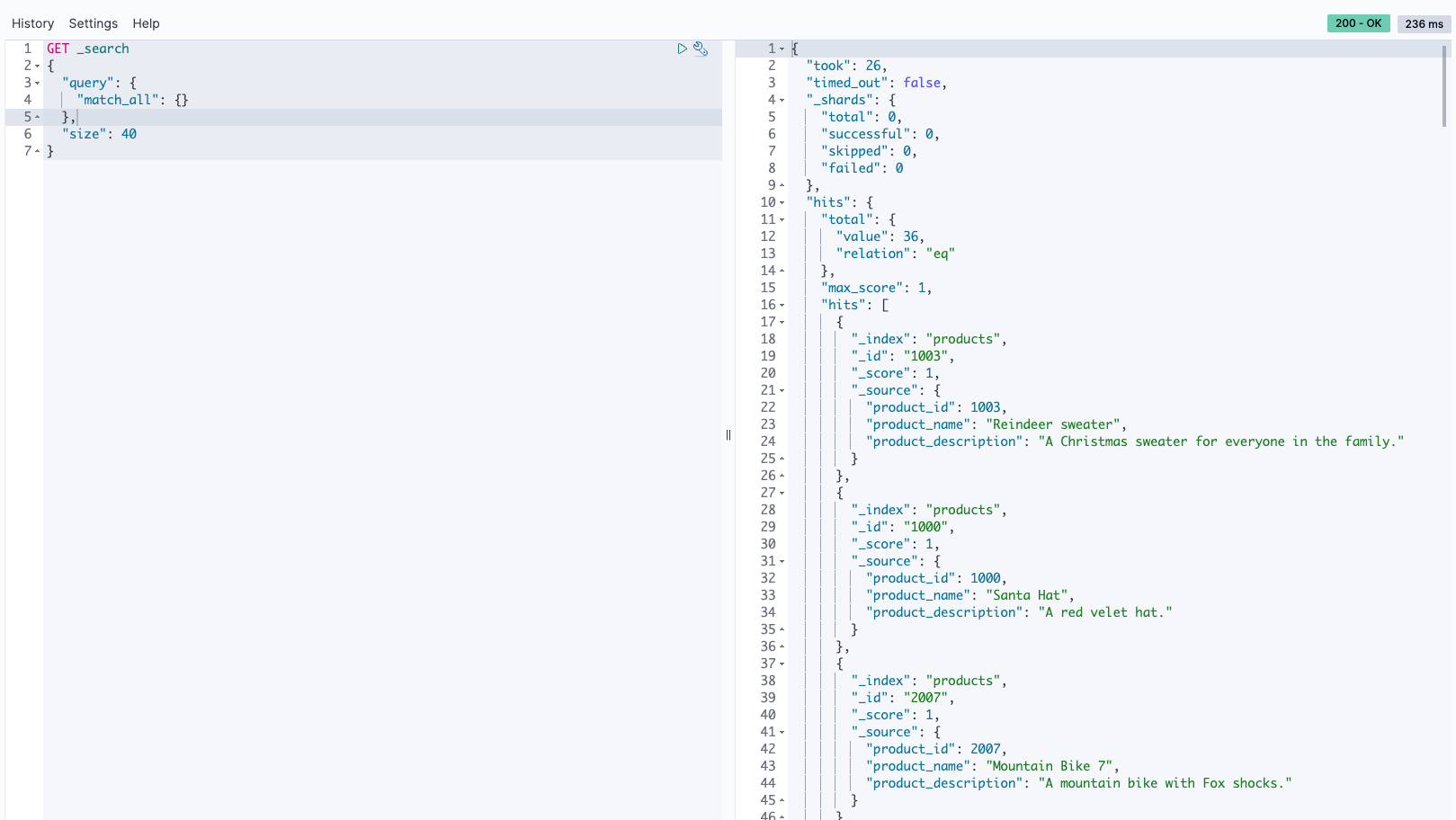
Ingest data into OpenSearch Service

If you’re using OpenSearch service, run the following script to ingest the files:

export AWS_REGION=$(curl -s http://169.254.169.254/latest/meta-data/placement/availability-zone | sed 's/\(.*\)[a-z]/\1/')
aws configure set region $AWS_REGION

python embedding_ray_os.py

When it’s complete, run the script that runs simulated queries:

python query_os.py

Ingest data into Amazon RDS

If you’re using Amazon RDS, run the following script to ingest the files:

export AWS_REGION=$(curl -s http://169.254.169.254/latest/meta-data/placement/availability-zone | sed 's/\(.*\)[a-z]/\1/')
aws configure set region $AWS_REGION

python embedding_ray_rds.py

When it’s complete, make sure to run a full vacuum on the RDS instance.

Then run the following script to run simulated queries:

python query_rds.py

Set up the Ray dashboard

Before you set up the Ray dashboard, you should install the AWS Command Line Interface (AWS CLI) on your local machine. For instructions, refer to Install or update the latest version of the AWS CLI.

Complete the following steps to set up the dashboard:

  1. Install the Session Manager plugin for the AWS CLI.
  2. In the Isengard account, copy the temporary credentials for bash/zsh and run in your local terminal.
  3. Create a session.sh file in your machine and copy the following content to the file:
#!/bin/bash
echo Starting session to $1 to forward to port $2 using local port $3
aws ssm start-session --target $1 --document-name AWS-StartPortForwardingSession --parameters ‘{“portNumber”:[“‘$2’“], “localPortNumber”:[“‘$3’“]}'
  1. Change the directory to where this session.sh file is stored.
  2. Run the command Chmod +x to give executable permission to the file.
  3. Run the following command:
./session.sh <Ray cluster head node instance ID> 8265 8265

For example:

./session.sh i-021821beb88661ba3 8265 8265

You will see a message like the following:

Starting session to i-021821beb88661ba3 to forward to port 8265 using local port 8265

Starting session with SessionId: abcdefgh-Isengard-0d73d992dfb16b146
Port 8265 opened for sessionId abcdefgh-Isengard-0d73d992dfb16b146.
Waiting for connections...

Open a new tab in your browser and enter localhost:8265.

You will see the Ray dashboard and statistics of the jobs and cluster running. You can track metrics from here.

For example, you can use the Ray dashboard to observe load on the cluster. As shown in the following screenshot, during ingest, the GPUs are running close to 100% utilization.

You can also use the RAG_Benchmarks CloudWatch dashboard to see the ingestion rate and query response times.

Extensibility of the solution

You can extend this solution to plug in other AWS or third-party vector stores. For every new vector store, you will need to create scripts for configuring the data store as well as ingesting data. The rest of the pipeline can be reused as needed.

Conclusion

In this post, we shared an ETL pipeline that you can use to put vectorized RAG data in both OpenSearch Service as well as Amazon RDS with the pgvector extension as vector datastores. The solution used a Ray cluster to provide the necessary parallelism to ingest a large data corpus. You can use this methodology to integrate any vector database of your choice to build RAG pipelines.


About the Authors

Randy DeFauw is a Senior Principal Solutions Architect at AWS. He holds an MSEE from the University of Michigan, where he worked on computer vision for autonomous vehicles. He also holds an MBA from Colorado State University. Randy has held a variety of positions in the technology space, ranging from software engineering to product management. He entered the big data space in 2013 and continues to explore that area. He is actively working on projects in the ML space and has presented at numerous conferences, including Strata and GlueCon.

David Christian is a Principal Solutions Architect based out of Southern California. He has his bachelor’s in Information Security and a passion for automation. His focus areas are DevOps culture and transformation, infrastructure as code, and resiliency. Prior to joining AWS, he held roles in security, DevOps, and system engineering, managing large-scale private and public cloud environments.

Prachi Kulkarni is a Senior Solutions Architect at AWS. Her specialization is machine learning, and she is actively working on designing solutions using various AWS ML, big data, and analytics offerings. Prachi has experience in multiple domains, including healthcare, benefits, retail, and education, and has worked in a range of positions in product engineering and architecture, management, and customer success.

Richa Gupta is a Solutions Architect at AWS. She is passionate about architecting end-to-end solutions for customers. Her specialization is machine learning and how it can be used to build new solutions that lead to operational excellence and drive business revenue. Prior to joining AWS, she worked in the capacity of a Software Engineer and Solutions Architect, building solutions for large telecom operators. Outside of work, she likes to explore new places and loves adventurous activities.

How the GoDaddy data platform achieved over 60% cost reduction and 50% performance boost by adopting Amazon EMR Serverless

Post Syndicated from Brandon Abear original https://aws.amazon.com/blogs/big-data/how-the-godaddy-data-platform-achieved-over-60-cost-reduction-and-50-performance-boost-by-adopting-amazon-emr-serverless/

This is a guest post co-written with Brandon Abear, Dinesh Sharma, John Bush, and Ozcan IIikhan from GoDaddy.

GoDaddy empowers everyday entrepreneurs by providing all the help and tools to succeed online. With more than 20 million customers worldwide, GoDaddy is the place people come to name their ideas, build a professional website, attract customers, and manage their work.

At GoDaddy, we take pride in being a data-driven company. Our relentless pursuit of valuable insights from data fuels our business decisions and ensures customer satisfaction. Our commitment to efficiency is unwavering, and we’ve undertaken an exciting initiative to optimize our batch processing jobs. In this journey, we have identified a structured approach that we refer to as the seven layers of improvement opportunities. This methodology has become our guide in the pursuit of efficiency.

In this post, we discuss how we enhanced operational efficiency with Amazon EMR Serverless. We share our benchmarking results and methodology, and insights into the cost-effectiveness of EMR Serverless vs. fixed capacity Amazon EMR on EC2 transient clusters on our data workflows orchestrated using Amazon Managed Workflows for Apache Airflow (Amazon MWAA). We share our strategy for the adoption of EMR Serverless in areas where it excels. Our findings reveal significant benefits, including over 60% cost reduction, 50% faster Spark workloads, a remarkable five-times improvement in development and testing speed, and a significant reduction in our carbon footprint.

Background

In late 2020, GoDaddy’s data platform initiated its AWS Cloud journey, migrating an 800-node Hadoop cluster with 2.5 PB of data from its data center to EMR on EC2. This lift-and-shift approach facilitated a direct comparison between on-premises and cloud environments, ensuring a smooth transition to AWS pipelines, minimizing data validation issues and migration delays.

By early 2022, we successfully migrated our big data workloads to EMR on EC2. Using best practices learned from the AWS FinHack program, we fine-tuned resource-intensive jobs, converted Pig and Hive jobs to Spark, and reduced our batch workload spend by 22.75% in 2022. However, scalability challenges emerged due to the multitude of jobs. This prompted GoDaddy to embark on a systematic optimization journey, establishing a foundation for more sustainable and efficient big data processing.

Seven layers of improvement opportunities

In our quest for operational efficiency, we have identified seven distinct layers of opportunities for optimization within our batch processing jobs, as shown in the following figure. These layers range from precise code-level enhancements to more comprehensive platform improvements. This multi-layered approach has become our strategic blueprint in the ongoing pursuit of better performance and higher efficiency.

Seven layers of improvement opportunities

The layers are as follows:

  • Code optimization – Focuses on refining the code logic and how it can be optimized for better performance. This involves performance enhancements through selective caching, partition and projection pruning, join optimizations, and other job-specific tuning. Using AI coding solutions is also an integral part of this process.
  • Software updates – Updating to the latest versions of open source software (OSS) to capitalize on new features and improvements. For example, Adaptive Query Execution in Spark 3 brings significant performance and cost improvements.
  • Custom Spark configurations Tuning of custom Spark configurations to maximize resource utilization, memory, and parallelism. We can achieve significant improvements by right-sizing tasks, such as through spark.sql.shuffle.partitions, spark.sql.files.maxPartitionBytes, spark.executor.cores, and spark.executor.memory. However, these custom configurations might be counterproductive if they are not compatible with the specific Spark version.
  • Resource provisioning time The time it takes to launch resources like ephemeral EMR clusters on Amazon Elastic Compute Cloud (Amazon EC2). Although some factors influencing this time are outside of an engineer’s control, identifying and addressing the factors that can be optimized can help reduce overall provisioning time.
  • Fine-grained scaling at task level Dynamically adjusting resources such as CPU, memory, disk, and network bandwidth based on each stage’s needs within a task. The aim here is to avoid fixed cluster sizes that could result in resource waste.
  • Fine-grained scaling across multiple tasks in a workflow Given that each task has unique resource requirements, maintaining a fixed resource size may result in under- or over-provisioning for certain tasks within the same workflow. Traditionally, the size of the largest task determines the cluster size for a multi-task workflow. However, dynamically adjusting resources across multiple tasks and steps within a workflow result in a more cost-effective implementation.
  • Platform-level enhancements – Enhancements at preceding layers can only optimize a given job or a workflow. Platform improvement aims to attain efficiency at the company level. We can achieve this through various means, such as updating or upgrading the core infrastructure, introducing new frameworks, allocating appropriate resources for each job profile, balancing service usage, optimizing the use of Savings Plans and Spot Instances, or implementing other comprehensive changes to boost efficiency across all tasks and workflows.

Layers 1–3: Previous cost reductions

After we migrated from on premises to AWS Cloud, we primarily focused our cost-optimization efforts on the first three layers shown in the diagram. By transitioning our most costly legacy Pig and Hive pipelines to Spark and optimizing Spark configurations for Amazon EMR, we achieved significant cost savings.

For example, a legacy Pig job took 10 hours to complete and ranked among the top 10 most expensive EMR jobs. Upon reviewing TEZ logs and cluster metrics, we discovered that the cluster was vastly over-provisioned for the data volume being processed and remained under-utilized for most of the runtime. Transitioning from Pig to Spark was more efficient. Although no automated tools were available for the conversion, manual optimizations were made, including:

  • Reduced unnecessary disk writes, saving serialization and deserialization time (Layer 1)
  • Replaced Airflow task parallelization with Spark, simplifying the Airflow DAG (Layer 1)
  • Eliminated redundant Spark transformations (Layer 1)
  • Upgraded from Spark 2 to 3, using Adaptive Query Execution (Layer 2)
  • Addressed skewed joins and optimized smaller dimension tables (Layer 3)

As a result, job cost decreased by 95%, and job completion time was reduced to 1 hour. However, this approach was labor-intensive and not scalable for numerous jobs.

Layers 4–6: Find and adopt the right compute solution

In late 2022, following our significant accomplishments in optimization at the previous levels, our attention moved towards enhancing the remaining layers.

Understanding the state of our batch processing

We use Amazon MWAA to orchestrate our data workflows in the cloud at scale. Apache Airflow is an open source tool used to programmatically author, schedule, and monitor sequences of processes and tasks referred to as workflows. In this post, the terms workflow and job are used interchangeably, referring to the Directed Acyclic Graphs (DAGs) consisting of tasks orchestrated by Amazon MWAA. For each workflow, we have sequential or parallel tasks, and even a combination of both in the DAG between create_emr and terminate_emr tasks running on a transient EMR cluster with fixed compute capacity throughout the workflow run. Even after optimizing a portion of our workload, we still had numerous non-optimized workflows that were under-utilized due to over-provisioning of compute resources based on the most resource-intensive task in the workflow, as shown in the following figure.

This highlighted the impracticality of static resource allocation and led us to recognize the necessity of a dynamic resource allocation (DRA) system. Before proposing a solution, we gathered extensive data to thoroughly understand our batch processing. Analyzing the cluster step time, excluding provisioning and idle time, revealed significant insights: a right-skewed distribution with over half of the workflows completing in 20 minutes or less and only 10% taking more than 60 minutes. This distribution guided our choice of a fast-provisioning compute solution, dramatically reducing workflow runtimes. The following diagram illustrates step times (excluding provisioning and idle time) of EMR on EC2 transient clusters in one of our batch processing accounts.

Furthermore, based on the step time (excluding provisioning and idle time) distribution of the workflows, we categorized our workflows into three groups:

  • Quick run – Lasting 20 minutes or less
  • Medium run – Lasting between 20–60 minutes
  • Long run – Exceeding 60 minutes, often spanning several hours or more

Another factor we needed to consider was the extensive use of transient clusters for reasons such as security, job and cost isolation, and purpose-built clusters. Additionally, there was a significant variation in resource needs between peak hours and periods of low utilization.

Instead of fixed-size clusters, we could potentially use managed scaling on EMR on EC2 to achieve some cost benefits. However, migrating to EMR Serverless appears to be a more strategic direction for our data platform. In addition to potential cost benefits, EMR Serverless offers additional advantages such as a one-click upgrade to the newest Amazon EMR versions, a simplified operational and debugging experience, and automatic upgrades to the latest generations upon rollout. These features collectively simplify the process of operating a platform on a larger scale.

Evaluating EMR Serverless: A case study at GoDaddy

EMR Serverless is a serverless option in Amazon EMR that eliminates the complexities of configuring, managing, and scaling clusters when running big data frameworks like Apache Spark and Apache Hive. With EMR Serverless, businesses can enjoy numerous benefits, including cost-effectiveness, faster provisioning, simplified developer experience, and improved resilience to Availability Zone failures.

Recognizing the potential of EMR Serverless, we conducted an in-depth benchmark study using real production workflows. The study aimed to assess EMR Serverless performance and efficiency while also creating an adoption plan for large-scale implementation. The findings were highly encouraging, showing EMR Serverless can effectively handle our workloads.

Benchmarking methodology

We split our data workflows into three categories based on total step time (excluding provisioning and idle time): quick run (0–20 minutes), medium run (20–60 minutes), and long run (over 60 minutes). We analyzed the impact of the EMR deployment type (Amazon EC2 vs. EMR Serverless) on two key metrics: cost-efficiency and total runtime speedup, which served as our overall evaluation criteria. Although we did not formally measure ease of use and resiliency, these factors were considered throughout the evaluation process.

The high-level steps to assess the environment are as follows:

  1. Prepare the data and environment:
    1. Choose three to five random production jobs from each job category.
    2. Implement required adjustments to prevent interference with production.
  2. Run tests:
    1. Run scripts over several days or through multiple iterations to gather precise and consistent data points.
    2. Perform tests using EMR on EC2 and EMR Serverless.
  3. Validate data and test runs:
    1. Validate input and output datasets, partitions, and row counts to ensure identical data processing.
  4. Gather metrics and analyze results:
    1. Gather relevant metrics from the tests.
    2. Analyze results to draw insights and conclusions.

Benchmark results

Our benchmark results showed significant enhancements across all three job categories for both runtime speedup and cost-efficiency. The improvements were most pronounced for quick jobs, directly resulting from faster startup times. For instance, a 20-minute (including cluster provisioning and shut down) data workflow running on an EMR on EC2 transient cluster of fixed compute capacity finishes in 10 minutes on EMR Serverless, providing a shorter runtime with cost benefits. Overall, the shift to EMR Serverless delivered substantial performance improvements and cost reductions at scale across job brackets, as seen in the following figure.

Historically, we devoted more time to tuning our long-run workflows. Interestingly, we discovered that the existing custom Spark configurations for these jobs did not always translate well to EMR Serverless. In cases where the results were insignificant, a common approach was to discard previous Spark configurations related to executor cores. By allowing EMR Serverless to autonomously manage these Spark configurations, we often observed improved outcomes. The following graph shows the average runtime and cost improvement per job when comparing EMR Serverless to EMR on EC2.

Per Job Improvement

The following table shows a sample comparison of results for the same workflow running on different deployment options of Amazon EMR (EMR on EC2 and EMR Serverless).

Metric EMR on EC2
(Average)
EMR Serverless
(Average)
EMR on EC2 vs
EMR Serverless
Total Run Cost ($) $ 5.82 $ 2.60 55%
Total Run Time (Minutes) 53.40 39.40 26%
Provisioning Time (Minutes) 10.20 0.05 .
Provisioning Cost ($) $ 1.19 . .
Steps Time (Minutes) 38.20 39.16 -3%
Steps Cost ($) $ 4.30 . .
Idle Time (Minutes) 4.80 . .
EMR Release Label emr-6.9.0 .
Hadoop Distribution Amazon 3.3.3 .
Spark Version Spark 3.3.0 .
Hive/HCatalog Version Hive 3.1.3, HCatalog 3.1.3 .
Job Type Spark .

AWS Graviton2 on EMR Serverless performance evaluation

After seeing compelling results with EMR Serverless for our workloads, we decided to further analyze the performance of the AWS Graviton2 (arm64) architecture within EMR Serverless. AWS had benchmarked Spark workloads on Graviton2 EMR Serverless using the TPC-DS 3TB scale, showing a 27% overall price-performance improvement.

To better understand the integration benefits, we ran our own study using GoDaddy’s production workloads on a daily schedule and observed an impressive 23.8% price-performance enhancement across a range of jobs when using Graviton2. For more details about this study, see GoDaddy benchmarking results in up to 24% better price-performance for their Spark workloads with AWS Graviton2 on Amazon EMR Serverless.

Adoption strategy for EMR Serverless

We strategically implemented a phased rollout of EMR Serverless via deployment rings, enabling systematic integration. This gradual approach let us validate improvements and halt further adoption of EMR Serverless, if needed. It served both as a safety net to catch issues early and a means to refine our infrastructure. The process mitigated change impact through smooth operations while building team expertise of our Data Engineering and DevOps teams. Additionally, it fostered tight feedback loops, allowing prompt adjustments and ensuring efficient EMR Serverless integration.

We divided our workflows into three main adoption groups, as shown in the following image:

  • Canaries This group aids in detecting and resolving any potential problems early in the deployment stage.
  • Early adopters This is the second batch of workflows that adopt the new compute solution after initial issues have been identified and rectified by the canaries group.
  • Broad deployment rings The largest group of rings, this group represents the wide-scale deployment of the solution. These are deployed after successful testing and implementation in the previous two groups.

Rings

We further broke down these workflows into granular deployment rings to adopt EMR Serverless, as shown in the following table.

Ring # Name Details
Ring 0 Canary Low adoption risk jobs that are expected to yield some cost saving benefits.
Ring 1 Early Adopters Low risk Quick-run Spark jobs that expect to yield high gains.
Ring 2 Quick-run Rest of the Quick-run (step_time <= 20 min) Spark jobs
Ring 3 LargerJobs_EZ High potential gain, easy move, medium-run and long-run Spark jobs
Ring 4 LargerJobs Rest of the medium-run and long-run Spark jobs with potential gains
Ring 5 Hive Hive jobs with potentially higher cost savings
Ring 6 Redshift_EZ Easy migration Redshift jobs that suit EMR Serverless
Ring 7 Glue_EZ Easy migration Glue jobs that suit EMR Serverless

Production adoption results summary

The encouraging benchmarking and canary adoption results generated considerable interest in wider EMR Serverless adoption at GoDaddy. To date, the EMR Serverless rollout remains underway. Thus far, it has reduced costs by 62.5% and accelerated total batch workflow completion by 50.4%.

Based on preliminary benchmarks, our team expected substantial gains for quick jobs. To our surprise, actual production deployments surpassed projections, averaging 64.4% faster vs. 42% projected, and 71.8% cheaper vs. 40% predicted.

Remarkably, long-running jobs also saw significant performance improvements due to the rapid provisioning of EMR Serverless and aggressive scaling enabled by dynamic resource allocation. We observed substantial parallelization during high-resource segments, resulting in a 40.5% faster total runtime compared to traditional approaches. The following chart illustrates the average enhancements per job category.

Prod Jobs Savings

Additionally, we observed the highest degree of dispersion for speed improvements within the long-run job category, as shown in the following box-and-whisker plot.

Whisker Plot

Sample workflows adopted EMR Serverless

For a large workflow migrated to EMR Serverless, comparing 3-week averages pre- and post-migration revealed impressive cost savings—a 75.30% decrease based on retail pricing with 10% improvement in total runtime, boosting operational efficiency. The following graph illustrates the cost trend.

Although quick-run jobs realized minimal per-dollar cost reductions, they delivered the most significant percentage cost savings. With thousands of these workflows running daily, the accumulated savings are substantial. The following graph shows the cost trend for a small workload migrated from EMR on EC2 to EMR Serverless. Comparing 3-week pre- and post-migration averages revealed a remarkable 92.43% cost savings on the retail on-demand pricing, alongside an 80.6% acceleration in total runtime.

Sample workflows adopted EMR Serverless 2

Layer 7: Platform-wide improvements

We aim to revolutionize compute operations at GoDaddy, providing simplified yet powerful solutions for all users with our Intelligent Compute Platform. With AWS compute solutions like EMR Serverless and EMR on EC2, it provided optimized runs of data processing and machine learning (ML) workloads. An ML-powered job broker intelligently determines when and how to run jobs based on various parameters, while still allowing power users to customize. Additionally, an ML-powered compute resource manager pre-provisions resources based on load and historical data, providing efficient, fast provisioning at optimum cost. Intelligent compute empowers users with out-of-the-box optimization, catering to diverse personas without compromising power users.

The following diagram shows a high-level illustration of the intelligent compute architecture.

Insights and recommended best-practices

The following section discusses the insights we’ve gathered and the recommended best practices we’ve developed during our preliminary and wider adoption stages.

Infrastructure preparation

Although EMR Serverless is a deployment method within EMR, it requires some infrastructure preparedness to optimize its potential. Consider the following requirements and practical guidance on implementation:

  • Use large subnets across multiple Availability Zones – When running EMR Serverless workloads within your VPC, make sure the subnets span across multiple Availability Zones and are not constrained by IP addresses. Refer to Configuring VPC access and Best practices for subnet planning for details.
  • Modify maximum concurrent vCPU quota For extensive compute requirements, it is recommended to increase your max concurrent vCPUs per account service quota.
  • Amazon MWAA version compatibility When adopting EMR Serverless, GoDaddy’s decentralized Amazon MWAA ecosystem for data pipeline orchestration created compatibility issues from disparate AWS Providers versions. Directly upgrading Amazon MWAA was more efficient than updating numerous DAGs. We facilitated adoption by upgrading Amazon MWAA instances ourselves, documenting issues, and sharing findings and effort estimates for accurate upgrade planning.
  • GoDaddy EMR operator To streamline migrating numerous Airflow DAGs from EMR on EC2 to EMR Serverless, we developed custom operators adapting existing interfaces. This allowed seamless transitions while retaining familiar tuning options. Data engineers could easily migrate pipelines with simple find-replace imports and immediately use EMR Serverless.

Unexpected behavior mitigation

The following are unexpected behaviors we ran into and what we did to mitigate them:

  • Spark DRA aggressive scaling For some jobs (8.33% of initial benchmarks, 13.6% of production), cost increased after migrating to EMR Serverless. This was due to Spark DRA excessively assigning new workers briefly, prioritizing performance over cost. To counteract this, we set maximum executor thresholds by adjusting spark.dynamicAllocation.maxExecutor, effectively limiting EMR Serverless scaling aggression. When migrating from EMR on EC2, we suggest observing the max core count in the Spark History UI to replicate similar compute limits in EMR Serverless, such as --conf spark.executor.cores and --conf spark.dynamicAllocation.maxExecutors.
  • Managing disk space for large-scale jobs When transitioning jobs that process large data volumes with substantial shuffles and significant disk requirements to EMR Serverless, we recommend configuring spark.emr-serverless.executor.disk by referring to existing Spark job metrics. Furthermore, configurations like spark.executor.cores combined with spark.emr-serverless.executor.disk and spark.dynamicAllocation.maxExecutors allow control over the underlying worker size and total attached storage when advantageous. For example, a shuffle-heavy job with relatively low disk usage may benefit from using a larger worker to increase the likelihood of local shuffle fetches.

Conclusion

As discussed in this post, our experiences with adopting EMR Serverless on arm64 have been overwhelmingly positive. The impressive results we’ve achieved, including a 60% reduction in cost, 50% faster runs of batch Spark workloads, and an astounding five-times improvement in development and testing speed, speak volumes about the potential of this technology. Furthermore, our current results suggest that by widely adopting Graviton2 on EMR Serverless, we could potentially reduce the carbon footprint by up to 60% for our batch processing.

However, it’s crucial to understand that these results are not a one-size-fits-all scenario. The enhancements you can expect are subject to factors including, but not limited to, the specific nature of your workflows, cluster configurations, resource utilization levels, and fluctuations in computational capacity. Therefore, we strongly advocate for a data-driven, ring-based deployment strategy when considering the integration of EMR Serverless, which can help optimize its benefits to the fullest.

Special thanks to Mukul Sharma and Boris Berlin for their contributions to benchmarking. Many thanks to Travis Muhlestein (CDO), Abhijit Kundu (VP Eng), Vincent Yung (Sr. Director Eng.), and Wai Kin Lau (Sr. Director Data Eng.) for their continued support.


About the Authors

Brandon Abear is a Principal Data Engineer in the Data & Analytics (DnA) organization at GoDaddy. He enjoys all things big data. In his spare time, he enjoys traveling, watching movies, and playing rhythm games.

Dinesh Sharma is a Principal Data Engineer in the Data & Analytics (DnA) organization at GoDaddy. He is passionate about user experience and developer productivity, always looking for ways to optimize engineering processes and saving cost. In his spare time, he loves reading and is an avid manga fan.

John Bush is a Principal Software Engineer in the Data & Analytics (DnA) organization at GoDaddy. He is passionate about making it easier for organizations to manage data and use it to drive their businesses forward. In his spare time, he loves hiking, camping, and riding his ebike.

Ozcan Ilikhan is the Director of Engineering for the Data and ML Platform at GoDaddy. He has over two decades of multidisciplinary leadership experience, spanning startups to global enterprises. He has a passion for leveraging data and AI in creating solutions that delight customers, empower them to achieve more, and boost operational efficiency. Outside of his professional life, he enjoys reading, hiking, gardening, volunteering, and embarking on DIY projects.

Harsh Vardhan is an AWS Solutions Architect, specializing in big data and analytics. He has over 8 years of experience working in the field of big data and data science. He is passionate about helping customers adopt best practices and discover insights from their data.

Real-time cost savings for Amazon Managed Service for Apache Flink

Post Syndicated from Jeremy Ber original https://aws.amazon.com/blogs/big-data/real-time-cost-savings-for-amazon-managed-service-for-apache-flink/

When running Apache Flink applications on Amazon Managed Service for Apache Flink, you have the unique benefit of taking advantage of its serverless nature. This means that cost-optimization exercises can happen at any time—they no longer need to happen in the planning phase. With Managed Service for Apache Flink, you can add and remove compute with the click of a button.

Apache Flink is an open source stream processing framework used by hundreds of companies in critical business applications, and by thousands of developers who have stream-processing needs for their workloads. It is highly available and scalable, offering high throughput and low latency for the most demanding stream-processing applications. These scalable properties of Apache Flink can be key to optimizing your cost in the cloud.

Managed Service for Apache Flink is a fully managed service that reduces the complexity of building and managing Apache Flink applications. Managed Service for Apache Flink manages the underlying infrastructure and Apache Flink components that provide durable application state, metrics, logs, and more.

In this post, you can learn about the Managed Service for Apache Flink cost model, areas to save on cost in your Apache Flink applications, and overall gain a better understanding of your data processing pipelines. We dive deep into understanding your costs, understanding whether your application is overprovisioned, how to think about scaling automatically, and ways to optimize your Apache Flink applications to save on cost. Lastly, we ask important questions about your workload to determine if Apache Flink is the right technology for your use case.

How costs are calculated on Managed Service for Apache Flink

To optimize for costs with regards to your Managed Service for Apache Flink application, it can help to have a good idea of what goes into the pricing for the managed service.

Managed Service for Apache Flink applications are comprised of Kinesis Processing Units (KPUs), which are compute instances composed of 1 virtual CPU and 4 GB of memory. The total number of KPUs assigned to the application is determined by multiplying two parameters that you control directly:

  • Parallelism – The level of parallel processing in the Apache Flink application
  • Parallelism per KPU – The number of resources dedicated to each parallelism

The number of KPUs is determined by the simple formula: KPU = Parallelism / ParallelismPerKPU, rounded up to the next integer.

An additional KPU per application is also charged for orchestration and not directly used for data processing.

The total number of KPUs determines the number of resources, CPU, memory, and application storage allocated to the application. For each KPU, the application receives 1 vCPU and 4 GB of memory, of which 3 GB are allocated by default to the running application and the remaining 1 GB is used for application state store management. Each KPU also comes with 50 GB of storage attached to the application. Apache Flink retains application state in-memory to a configurable limit, and spillover to the attached storage.

The third cost component is durable application backups, or snapshots. This is entirely optional and its impact on the overall cost is small, unless you retain a very large number of snapshots.

At the time of writing, each KPU in the US East (Ohio) AWS Region costs $0.11 per hour, and attached application storage costs $0.10 per GB per month. The cost of durable application backup (snapshots) is $0.023 per GB per month. Refer to Amazon Managed Service for Apache Flink Pricing for up-to-date pricing and different Regions.

The following diagram illustrates the relative proportions of cost components for a running application on Managed Service for Apache Flink. You control the number of KPUs via the parallelism and parallelism per KPU parameters. Durable application backup storage is not represented.

pricing model

In the following sections, we examine how to monitor your costs, optimize the usage of application resources, and find the required number of KPUs to handle your throughput profile.

AWS Cost Explorer and understanding your bill

To see what your current Managed Service for Apache Flink spend is, you can use AWS Cost Explorer.

On the Cost Explorer console, you can filter by date range, usage type, and service to isolate your spend for Managed Service for Apache Flink applications. The following screenshot shows the past 12 months of cost broken down into the price categories described in the previous section. The majority of spend in many of these months was from interactive KPUs from Amazon Managed Service for Apache Flink Studio.

Analyse the cost of your Apache Flink application with AWS Cost Explorer

Using Cost Explorer can not only help you understand your bill, but help further optimize particular applications that may have scaled beyond expectations automatically or due to throughput requirements. With proper application tagging, you could also break this spend down by application to see which applications account for the cost.

Signs of overprovisioning or inefficient use of resources

To minimize costs associated with Managed Service for Apache Flink applications, a straightforward approach involves reducing the number of KPUs your applications use. However, it’s crucial to recognize that this reduction could adversely affect performance if not thoroughly assessed and tested. To quickly gauge whether your applications might be overprovisioned, examine key indicators such as CPU and memory usage, application functionality, and data distribution. However, although these indicators can suggest potential overprovisioning, it’s essential to conduct performance testing and validate your scaling patterns before making any adjustments to the number of KPUs.

Metrics

Analyzing metrics for your application on Amazon CloudWatch can reveal clear signals of overprovisioning. If the containerCPUUtilization and containerMemoryUtilization metrics consistently remain below 20% over a statistically significant period for your application’s traffic patterns, it might be viable to scale down and allocate more data to fewer machines. Generally, we consider applications appropriately sized when containerCPUUtilization hovers between 50–75%. Although containerMemoryUtilization can fluctuate throughout the day and be influenced by code optimization, a consistently low value for a substantial duration could indicate potential overprovisioning.

Parallelism per KPU underutilized

Another subtle sign that your application is overprovisioned is if your application is purely I/O bound, or only does simple call-outs to databases and non-CPU intensive operations. If this is the case, you can use the parallelism per KPU parameter within Managed Service for Apache Flink to load more tasks onto a single processing unit.

You can view the parallelism per KPU parameter as a measure of density of workload per unit of compute and memory resources (the KPU). Increasing parallelism per KPU above the default value of 1 makes the processing more dense, allocating more parallel processes on a single KPU.

The following diagram illustrates how, by keeping the application parallelism constant (for example, 4) and increasing parallelism per KPU (for example, from 1 to 2), your application uses fewer resources with the same level of parallel runs.

How KPUs are calculated

The decision of increasing parallelism per KPU, like all recommendations in this post, should be taken with great care. Increasing the parallelism per KPU value can put more load on a single KPU, and it must be willing to tolerate that load. I/O-bound operations will not increase CPU or memory utilization in any meaningful way, but a process function that calculates many complex operations against the data would not be an ideal operation to collate onto a single KPU, because it could overwhelm the resources. Performance test and evaluate if this is a good option for your applications.

How to approach sizing

Before you stand up a Managed Service for Apache Flink application, it can be difficult to estimate the number of KPUs you should allocate for your application. In general, you should have a good sense of your traffic patterns before estimating. Understanding your traffic patterns on a megabyte-per-second ingestion rate basis can help you approximate a starting point.

As a general rule, you can start with one KPU per 1 MB/s that your application will process. For example, if your application processes 10 MB/s (on average), you would allocate 10 KPUs as a starting point for your application. Keep in mind that this is a very high-level approximation that we have seen effective for a general estimate. However, you also need to performance test and evaluate whether or not this is an appropriate sizing in the long term based on metrics (CPU, memory, latency, overall job performance) over a long period of time.

To find the appropriate sizing for your application, you need to scale up and down the Apache Flink application. As mentioned, in Managed Service for Apache Flink you have two separate controls: parallelism and parallelism per KPU. Together, these parameters determine the level of parallel processing within the application and the overall compute, memory, and storage resources available.

The recommended testing methodology is to change parallelism or parallelism per KPU separately, while experimenting to find the right sizing. In general, only change parallelism per KPU to increase the number of parallel I/O-bound operations, without increasing the overall resources. For all other cases, only change parallelism—KPU will change consequentially—to find the right sizing for your workload.

You can also set parallelism at the operator level to restrict sources, sinks, or any other operator that might need to be restricted and independent of scaling mechanisms. You could use this for an Apache Flink application that reads from an Apache Kafka topic that has 10 partitions. With the setParallelism() method, you could restrict the KafkaSource to 10, but scale the Managed Service for Apache Flink application to a parallelism higher than 10 without creating idle tasks for the Kafka source. It is recommended for other data processing cases to not statically set operator parallelism to a static value, but rather a function of the application parallelism so that it scales when the overall application scales.

Scaling and auto scaling

In Managed Service for Apache Flink, modifying parallelism or parallelism per KPU is an update of the application configuration. It causes the application to automatically take a snapshot (unless disabled), stop the application, and restart it with the new sizing, restoring the state from the snapshot. Scaling operations don’t cause data loss or inconsistencies, but it does pause data processing for a short period of time while infrastructure is added or removed. This is something you need to consider when rescaling in a production environment.

During the testing and optimization process, we recommend disabling automatic scaling and modifying parallelism and parallelism per KPU to find the optimal values. As mentioned, manual scaling is just an update of the application configuration, and can be run via the AWS Management Console or API with the UpdateApplication action.

When you have found the optimal sizing, if you expect your ingested throughput to vary considerably, you may decide to enable auto scaling.

In Managed Service for Apache Flink, you can use multiple types of automatic scaling:

  • Out-of-the-box automatic scaling – You can enable this to adjust the application parallelism automatically based on the containerCPUUtilization metric. Automatic scaling is enabled by default on new applications. For details about the automatic scaling algorithm, refer to Automatic Scaling.
  • Fine-grained, metric-based automatic scaling – This is straightforward to implement. The automation can be based on virtually any metrics, including custom metrics your application exposes.
  • Scheduled scaling – This may be useful if you expect peaks of workload at given times of the day or days of the week.

Out-of-the-box automatic scaling and fine-grained metric-based scaling are mutually exclusive. For more details about fine-grained metric-based auto scaling and scheduled scaling, and a fully working code example, refer to Enable metric-based and scheduled scaling for Amazon Managed Service for Apache Flink.

Code optimizations

Another way to approach cost savings for your Managed Service for Apache Flink applications is through code optimization. Un-optimized code will require more machines to perform the same computations. Optimizing the code could allow for lower overall resource utilization, which in turn could allow for scaling down and cost savings accordingly.

The first step to understanding your code performance is through the built-in utility within Apache Flink called Flame Graphs.

Flame graph

Flame Graphs, which are accessible via the Apache Flink dashboard, give you a visual representation of your stack trace. Each time a method is called, the bar that represents that method call in the stack trace gets larger proportional to the total sample count. This means that if you have an inefficient piece of code with a very long bar in the flame graph, this could be cause for investigation as to how to make this code more efficient. Additionally, you can use Amazon CodeGuru Profiler to monitor and optimize your Apache Flink applications running on Managed Service for Apache Flink.

When designing your applications, it is recommended to use the highest-level API that is required for a particular operation at a given time. Apache Flink offers four levels of API support: Flink SQL, Table API, Datastream API, and ProcessFunction APIs, with increasing levels of complexity and responsibility. If your application can be written entirely in the Flink SQL or Table API, using this can help take advantage of the Apache Flink framework rather than managing state and computations manually.

Data skew

On the Apache Flink dashboard, you can gather other useful information about your Managed Service for Apache Flink jobs.

Open the Flink Dashboard

On the dashboard, you can inspect individual tasks within your job application graph. Each blue box represents a task, and each task is composed of subtasks, or distributed units of work for that task. You can identify data skew among subtasks this way.

Flink dashboard

Data skew is an indicator that more data is being sent to one subtask than another, and that a subtask receiving more data is doing more work than the other. If you have such symptoms of data skew, you can work to eliminate it by identifying the source. For example, a GroupBy or KeyedStream could have a skew in the key. This would mean that data is not evenly spread among keys, resulting in an uneven distribution of work across Apache Flink compute instances. Imagine a scenario where you are grouping by userId, but your application receives data from one user significantly more than the rest. This can result in data skew. To eliminate this, you can choose a different grouping key to evenly distribute the data across subtasks. Keep in mind that this will require code modification to choose a different key.

When the data skew is eliminated, you can return to the containerCPUUtilization and containerMemoryUtilization metrics to reduce the number of KPUs.

Other areas for code optimization include making sure that you’re accessing external systems via the Async I/O API or via a data stream join, because a synchronous query out to a data store can create slowdowns and issues in checkpointing. Additionally, refer to Troubleshooting Performance for issues you might experience with slow checkpoints or logging, which can cause application backpressure.

How to determine if Apache Flink is the right technology

If your application doesn’t use any of the powerful capabilities behind the Apache Flink framework and Managed Service for Apache Flink, you could potentially save on cost by using something simpler.

Apache Flink’s tagline is “Stateful Computations over Data Streams.” Stateful, in this context, means that you are using the Apache Flink state construct. State, in Apache Flink, allows you to remember messages you have seen in the past for longer periods of time, making things like streaming joins, deduplication, exactly-once processing, windowing, and late-data handling possible. It does so by using an in-memory state store. On Managed Service for Apache Flink, it uses RocksDB to maintain its state.

If your application doesn’t involve stateful operations, you may consider alternatives such as AWS Lambda, containerized applications, or an Amazon Elastic Compute Cloud (Amazon EC2) instance running your application. The complexity of Apache Flink may not be necessary in such cases. Stateful computations, including cached data or enrichment procedures requiring independent stream position memory, may warrant Apache Flink’s stateful capabilities. If there’s a potential for your application to become stateful in the future, whether through prolonged data retention or other stateful requirements, continuing to use Apache Flink could be more straightforward. Organizations emphasizing Apache Flink for stream processing capabilities may prefer to stick with Apache Flink for stateful and stateless applications so all their applications process data in the same way. You should also factor in its orchestration features like exactly-once processing, fan-out capabilities, and distributed computation before transitioning from Apache Flink to alternatives.

Another consideration is your latency requirements. Because Apache Flink excels at real-time data processing, using it for an application with a 6-hour or 1-day latency requirement does not make sense. The cost savings by switching to a temporal batch process out of Amazon Simple Storage Service (Amazon S3), for example, would be significant.

Conclusion

In this post, we covered some aspects to consider when attempting cost-savings measures for Managed Service for Apache Flink. We discussed how to identify your overall spend on the managed service, some useful metrics to monitor when scaling down your KPUs, how to optimize your code for scaling down, and how to determine if Apache Flink is right for your use case.

Implementing these cost-saving strategies not only enhances your cost efficiency but also provides a streamlined and well-optimized Apache Flink deployment. By staying mindful of your overall spend, using key metrics, and making informed decisions about scaling down resources, you can achieve a cost-effective operation without compromising performance. As you navigate the landscape of Apache Flink, constantly evaluating whether it aligns with your specific use case becomes pivotal, so you can achieve a tailored and efficient solution for your data processing needs.

If any of the recommendations discussed in this post resonate with your workloads, we encourage you to try them out. With the metrics specified, and the tips on how to understand your workloads better, you should now have what you need to efficiently optimize your Apache Flink workloads on Managed Service for Apache Flink. The following are some helpful resources you can use to supplement this post:


About the Authors

Jeremy BerJeremy Ber has been working in the telemetry data space for the past 10 years as a Software Engineer, Machine Learning Engineer, and most recently a Data Engineer. At AWS, he is a Streaming Specialist Solutions Architect, supporting both Amazon Managed Streaming for Apache Kafka (Amazon MSK) and Amazon Managed Service for Apache Flink.

Lorenzo NicoraLorenzo Nicora works as Senior Streaming Solution Architect at AWS, helping customers across EMEA. He has been building cloud-native, data-intensive systems for over 25 years, working in the finance industry both through consultancies and for FinTech product companies. He has leveraged open-source technologies extensively and contributed to several projects, including Apache Flink.

In-stream anomaly detection with Amazon OpenSearch Ingestion and Amazon OpenSearch Serverless

Post Syndicated from Rupesh Tiwari original https://aws.amazon.com/blogs/big-data/in-stream-anomaly-detection-with-amazon-opensearch-ingestion-and-amazon-opensearch-serverless/

Unsupervised machine learning analytics has emerged as a powerful tool for anomaly detection in today’s data-rich landscape, especially with the growing volume of machine-generated data. In-stream anomaly detection offers real-time insights into data anomalies, enabling proactive response. Amazon OpenSearch Serverless focuses on delivering seamless scalability and management of search workloads; Amazon OpenSearch Ingestion complements this by providing a robust solution for anomaly detection on indexed data.

In this post, we provide a solution using OpenSearch Ingestion that empowers you to perform in-stream anomaly detection within your own AWS environment.

In-stream anomaly detection with OpenSearch Ingestion

OpenSearch Ingestion makes the process of in-stream anomaly detection straightforward and at less cost. In-stream anomaly detection helps you save on indexing and avoids the need for extensive resources to handle big data. It lets organizations apply the appropriate resources at the appropriate time, managing large data efficiently and saving money. Using peer forwarders and aggregate processors can make things more complex and expensive; OpenSearch Ingestion reduces these issues.

Let’s look at a use case showing an OpenSearch Ingestion configuration YAML for in-stream anomaly detection.

Solution overview

In this example, we walk through the setup of OpenSearch Ingestion using a random cut forest anomaly detector for monitoring log counts within a 5-minute period. We also index the raw logs to provide a comprehensive demonstration of the incoming data flow. If your use case requires the analysis of raw logs, you can streamline the process by bypassing the initial pipeline and focus directly on in-stream anomaly detection, indexing only the identified anomalies.

The following diagram illustrates our solution architecture.

The configuration outlines two OpenSearch Ingestion pipelines. The first, non-ad-pipeline, ingests HTTP data, timestamps it, and forwards it to both ad-pipeline and an OpenSearch index, non-ad-index. The second, ad-pipeline, receives this data, performs aggregation based on the ID within a 5-minute window, and conducts anomaly detection. Results are stored in the index ad-anomaly-index. This setup showcases data processing, anomaly detection, and storage within OpenSearch Service, enhancing analysis capabilities.

Implement the solution

Complete the following steps to set up the solution:

  1. Create a pipeline role.
  2. Create a collection.
  3. Create a pipeline in which you specify the pipeline role.

The pipeline assumes this role in order to sign requests to the OpenSearch Serverless collection endpoint. Specify the values for the keys within the following pipeline configuration:

  • For sts_role_arn, specify the Amazon Resource Name (ARN) of the pipeline role that you created.
  • For hosts, specify the endpoint of the collection that you created.
  • Set serverless to true.
version: "2"
# 1st pipeline
non-ad-pipeline:
  source:
    http:
      path: "/${pipelineName}/test_ingestion_path"
  processor:
    - date:
        from_time_received: true
        destination: "@timestamp"
  sink:
    - pipeline:
        name: "ad-pipeline"
    - opensearch:
        hosts:
          [
            "https://{collection-id}.us-east-1.aoss.amazonaws.com",
          ]
        index: "non-ad-index"
        
        aws:
          sts_role_arn: "arn:aws:iam::{account-id}:role/pipeline-role"
          region: "us-east-1"
          serverless: true
# 2nd pipeline
ad-pipeline:
  source:
    pipeline:
      name: "non-ad-pipeline"
  processor:
    - aggregate:
        identification_keys: ["id"]
        action:
          count:
        group_duration: "300s"
    - anomaly_detector:
        keys: ["value"] # value will have sum of logs
        mode:
          random_cut_forest:
            output_after: 200 
  sink:
    - opensearch:
        hosts:
          [
            "https://{collection-id}.us-east-1.aoss.amazonaws.com",
          ]
        aws:
          sts_role_arn: "arn:aws:iam::{account-id}:role/pipeline-role"
          region: "us-east-1"
          serverless: true
        index: "ad-anomaly-index"

For a detailed guide on the required parameters and any limitations, see Supported plugins and options for Amazon OpenSearch Ingestion pipelines.

  1. After you update the configuration, confirm the validity of your pipeline settings by choosing Validate pipeline.

A successful validation will display a message stating Pipeline configuration validation successful.” as shown in the following screenshot.

If validation fails, refer to Troubleshooting Amazon OpenSearch Service for troubleshooting and guidance.

Cost estimation for OpenSearch Ingestion

You are only charged for the number of Ingestion OpenSearch Compute Units (Ingestion OCUs) that are allocated to a pipeline, regardless of whether there’s data flowing through the pipeline. OpenSearch Ingestion immediately accommodates your workloads by scaling pipeline capacity up or down based on usage. For an overview of expenses, refer to Amazon OpenSearch Ingestion.

The following table shows approximate monthly costs based on specified throughputs and compute needs. Let’s assume that operation occurs from 8:00 AM to 8:00 PM on weekdays, with a cost of $0.24 per OCU per hour.

The formula would be: Total Cost/Month = OCU Requirement * OCU Price * Hours/Day * Days/Month.

Throughput Compute Required (OCUs) Total Cost/Month (USD)
1 Gbps 10 576
10 Gbps 100 5760
50 Gbps 500 28800
100 Gbps 1000 57600
500 Gbps 5000 288000

Clean up

When you are done using the solution, delete the resources you created, including the pipeline role, pipeline, and collection.

Summary

With OpenSearch Ingestion, you can explore in-stream anomaly detection with OpenSearch Service. The use case in this post demonstrates how OpenSearch Ingestion simplifies the process, achieving more with fewer resources. It showcases the service’s ability to analyze log rates, generate anomaly notifications, and empower proactive response to anomalies. With OpenSearch Ingestion, you can improve operational efficiency and enhance real-time risk management capabilities.

Leave any thoughts and questions in the comments.


About the Authors

Rupesh Tiwari, an AWS Solutions Architect, specializes in modernizing applications with a focus on data analytics, OpenSearch, and generative AI. He’s known for creating scalable, secure solutions that leverage cloud technology for transformative business outcomes, also dedicating time to community engagement and sharing expertise.

Muthu Pitchaimani is a Search Specialist with Amazon OpenSearch Service. He builds large-scale search applications and solutions. Muthu is interested in the topics of networking and security, and is based out of Austin, Texas.

Petabyte-scale log analytics with Amazon S3, Amazon OpenSearch Service, and Amazon OpenSearch Ingestion

Post Syndicated from Jagadish Kumar original https://aws.amazon.com/blogs/big-data/petabyte-scale-log-analytics-with-amazon-s3-amazon-opensearch-service-and-amazon-opensearch-ingestion/

Organizations often need to manage a high volume of data that is growing at an extraordinary rate. At the same time, they need to optimize operational costs to unlock the value of this data for timely insights and do so with a consistent performance.

With this massive data growth, data proliferation across your data stores, data warehouse, and data lakes can become equally challenging. With a modern data architecture on AWS, you can rapidly build scalable data lakes; use a broad and deep collection of purpose-built data services; ensure compliance via unified data access, security, and governance; scale your systems at a low cost without compromising performance; and share data across organizational boundaries with ease, allowing you to make decisions with speed and agility at scale.

You can take all your data from various silos, aggregate that data in your data lake, and perform analytics and machine learning (ML) directly on top of that data. You can also store other data in purpose-built data stores to analyze and get fast insights from both structured and unstructured data. This data movement can be inside-out, outside-in, around the perimeter or sharing across.

For example, application logs and traces from web applications can be collected directly in a data lake, and a portion of that data can be moved out to a log analytics store like Amazon OpenSearch Service for daily analysis. We think of this concept as inside-out data movement. The analyzed and aggregated data stored in Amazon OpenSearch Service can again be moved to the data lake to run ML algorithms for downstream consumption from applications. We refer to this concept as outside-in data movement.

Let’s look at an example use case. Example Corp. is a leading Fortune 500 company that specializes in social content. They have hundreds of applications generating data and traces at approximately 500 TB per day and have the following criteria:

  • Have logs available for fast analytics for 2 days
  • Beyond 2 days, have data available in a storage tier that can be made available for analytics with a reasonable SLA
  • Retain the data beyond 1 week in cold storage for 30 days (for purposes of compliance, auditing, and others)

In the following sections, we discuss three possible solutions to address similar use cases:

  • Tiered storage in Amazon OpenSearch Service and data lifecycle management
  • On-demand ingestion of logs using Amazon OpenSearch Ingestion
  • Amazon OpenSearch Service direct queries with Amazon Simple Storage Service (Amazon S3)

Solution 1: Tiered storage in OpenSearch Service and data lifecycle management

OpenSearch Service supports three integrated storage tiers: hot, UltraWarm, and cold storage. Based on your data retention, query latency, and budgeting requirements, you can choose the best strategy to balance cost and performance. You can also migrate data between different storage tiers.

Hot storage is used for indexing and updating, and provides the fastest access to data. Hot storage takes the form of an instance store or Amazon Elastic Block Store (Amazon EBS) volumes attached to each node.

UltraWarm offers significantly lower costs per GiB for read-only data that you query less frequently and doesn’t need the same performance as hot storage. UltraWarm nodes use Amazon S3 with related caching solutions to improve performance.

Cold storage is optimized to store infrequently accessed or historical data. When you use cold storage, you detach your indexes from the UltraWarm tier, making them inaccessible. You can reattach these indexes in a few seconds when you need to query that data.

For more details on data tiers within OpenSearch Service, refer to Choose the right storage tier for your needs in Amazon OpenSearch Service.

Solution overview

The workflow for this solution consists of the following steps:

  1. Incoming data generated by the applications is streamed to an S3 data lake.
  2. Data is ingested into Amazon OpenSearch using S3-SQS near-real-time ingestion through notifications set up on the S3 buckets.
  3. After 2 days, hot data is migrated to UltraWarm storage to support read queries.
  4. After 5 days in UltraWarm, the data is migrated to cold storage for 21 days and detached from any compute. The data can be reattached to UltraWarm when needed. Data is deleted from cold storage after 21 days.
  5. Daily indexes are maintained for easy rollover. An Index State Management (ISM) policy automates the rollover or deletion of indexes that are older than 2 days.

The following is a sample ISM policy that rolls over data into the UltraWarm tier after 2 days, moves it to cold storage after 5 days, and deletes it from cold storage after 21 days:

{
    "policy": {
        "description": "hot warm delete workflow",
        "default_state": "hot",
        "schema_version": 1,
        "states": [
            {
                "name": "hot",
                "actions": [
                    {
                        "rollover": {
                            "min_index_age": "2d",
                            "min_primary_shard_size": "30gb"
                        }
                    }
                ],
                "transitions": [
                    {
                        "state_name": "warm"
                    }
                ]
            },
            {
                "name": "warm",
                "actions": [
                    {
                        "replica_count": {
                            "number_of_replicas": 5
                        }
                    }
                ],
                "transitions": [
                    {
                        "state_name": "cold",
                        "conditions": {
                            "min_index_age": "5d"
                        }
                    }
                ]
            },
            {
                "name": "cold",
                "actions": [
                    {
                        "retry": {
                            "count": 5,
                            "backoff": "exponential",
                            "delay": "1h"
                        },
                        "cold_migration": {
                            "start_time": null,
                            "end_time": null,
                            "timestamp_field": "@timestamp",
                            "ignore": "none"
                        }
                    }
                ],
                "transitions": [
                    {
                        "state_name": "delete",
                        "conditions": {
                            "min_index_age": "21d"
                        }
                    }
                ]
            },
            {
                "name": "delete",
                "actions": [
                    {
                        "retry": {
                            "count": 3,
                            "backoff": "exponential",
                            "delay": "1m"
                        },
                        "cold_delete": {}
                    }
                ],
                "transitions": []
            }
        ],
        "ism_template": {
            "index_patterns": [
                "log*"
            ],
            "priority": 100
        }
    }
}

Considerations

UltraWarm uses sophisticated caching techniques to enable querying for infrequently accessed data. Although the data access is infrequent, the compute for UltraWarm nodes needs to be running all the time to make this access possible.

When operating at PB scale, to reduce the area of effect of any errors, we recommend decomposing the implementation into multiple OpenSearch Service domains when using tiered storage.

The next two patterns remove the need to have long-running compute and describe on-demand techniques where the data is either brought when needed or queried directly where it resides.

Solution 2: On-demand ingestion of logs data through OpenSearch Ingestion

OpenSearch Ingestion is a fully managed data collector that delivers real-time log and trace data to OpenSearch Service domains. OpenSearch Ingestion is powered by the open source data collector Data Prepper. Data Prepper is part of the open source OpenSearch project.

With OpenSearch Ingestion, you can filter, enrich, transform, and deliver your data for downstream analysis and visualization. You configure your data producers to send data to OpenSearch Ingestion. It automatically delivers the data to the domain or collection that you specify. You can also configure OpenSearch Ingestion to transform your data before delivering it. OpenSearch Ingestion is serverless, so you don’t need to worry about scaling your infrastructure, operating your ingestion fleet, and patching or updating the software.

There are two ways that you can use Amazon S3 as a source to process data with OpenSearch Ingestion. The first option is S3-SQS processing. You can use S3-SQS processing when you require near-real-time scanning of files after they are written to S3. It requires an Amazon Simple Queue Service (Amazon S3) queue that receives S3 Event Notifications. You can configure S3 buckets to raise an event any time an object is stored or modified within the bucket to be processed.

Alternatively, you can use a one-time or recurring scheduled scan to batch process data in an S3 bucket. To set up a scheduled scan, configure your pipeline with a schedule at the scan level that applies to all your S3 buckets, or at the bucket level. You can configure scheduled scans with either a one-time scan or a recurring scan for batch processing.

For a comprehensive overview of OpenSearch Ingestion, see Amazon OpenSearch Ingestion. For more information about the Data Prepper open source project, visit Data Prepper.

Solution overview

We present an architecture pattern with the following key components:

  • Application logs are streamed into to the data lake, which helps feed hot data into OpenSearch Service in near-real time using OpenSearch Ingestion S3-SQS processing.
  • ISM policies within OpenSearch Service handle index rollovers or deletions. ISM policies let you automate these periodic, administrative operations by triggering them based on changes in the index age, index size, or number of documents. For example, you can define a policy that moves your index into a read-only state after 2 days and then deletes it after a set period of 3 days.
  • Cold data is available in the S3 data lake to be consumed on demand into OpenSearch Service using OpenSearch Ingestion scheduled scans.

The following diagram illustrates the solution architecture.

The workflow includes the following steps:

  1. Incoming data generated by the applications is streamed to the S3 data lake.
  2. For the current day, data is ingested into OpenSearch Service using S3-SQS near-real-time ingestion through notifications set up in the S3 buckets.
  3. Daily indexes are maintained for easy rollover. An ISM policy automates the rollover or deletion of indexes that are older than 2 days.
  4. If a request is made for analysis of data beyond 2 days and the data is not in the UltraWarm tier, data will be ingested using the one-time scan feature of Amazon S3 between the specific time window.

For example, if the present day is January 10, 2024, and you need data from January 6, 2024 at a specific interval for analysis, you can create an OpenSearch Ingestion pipeline with an Amazon S3 scan in your YAML configuration, with the start_time and end_time to specify when you want the objects in the bucket to be scanned:

version: "2"
ondemand-ingest-pipeline:
  source:
    s3:
      codec:
        newline:
      compression: "gzip"
      scan:
        start_time: 2023-12-28T01:00:00
        end_time: 2023-12-31T09:00:00
        buckets:
          - bucket:
              name: <bucket-name>
      aws:
        region: "us-east-1"
        sts_role_arn: "arn:aws:iam::<acct num>:role/PipelineRole"
    
    acknowledgments: true
  processor:
    - parse_json:
    - date:
        from_time_received: true
        destination: "@timestamp"           
  sink:
    - opensearch:                  
        index: "logs_ondemand_20231231"
        hosts: [ "https://search-XXXX-domain-XXXXXXXXXX.us-east-1.es.amazonaws.com" ]
        aws:                  
          sts_role_arn: "arn:aws:iam::<acct num>:role/PipelineRole"
          region: "us-east-1"

Considerations

Take advantage of compression

Data in Amazon S3 can be compressed, which reduces your overall data footprint and results in significant cost savings. For example, if you are generating 15 PB of raw JSON application logs per month, you can use a compression mechanism like GZIP, which can reduce the size to approximately 1PB or less, resulting in significant cost savings.

Stop the pipeline when possible

OpenSearch Ingestion scales automatically between the minimum and maximum OCUs set for the pipeline. After the pipeline has completed the Amazon S3 scan for the specified duration mentioned in the pipeline configuration, the pipeline continues to run for continuous monitoring at the minimum OCUs.

For on-demand ingestion for past time durations where you don’t expect new objects to be created, consider using supported pipeline metrics such as recordsOut.count to create Amazon CloudWatch alarms that can stop the pipeline. For a list of supported metrics, refer to Monitoring pipeline metrics.

CloudWatch alarms perform an action when a CloudWatch metric exceeds a specified value for some amount of time. For example, you might want to monitor recordsOut.count to be 0 for longer than 5 minutes to initiate a request to stop the pipeline through the AWS Command Line Interface (AWS CLI) or API.

Solution 3: OpenSearch Service direct queries with Amazon S3

OpenSearch Service direct queries with Amazon S3 (preview) is a new way to query operational logs in Amazon S3 and S3 data lakes without needing to switch between services. You can now analyze infrequently queried data in cloud object stores and simultaneously use the operational analytics and visualization capabilities of OpenSearch Service.

OpenSearch Service direct queries with Amazon S3 provides zero-ETL integration to reduce the operational complexity of duplicating data or managing multiple analytics tools by enabling you to directly query your operational data, reducing costs and time to action. This zero-ETL integration is configurable within OpenSearch Service, where you can take advantage of various log type templates, including predefined dashboards, and configure data accelerations tailored to that log type. Templates include VPC Flow Logs, Elastic Load Balancing logs, and NGINX logs, and accelerations include skipping indexes, materialized views, and covered indexes.

With OpenSearch Service direct queries with Amazon S3, you can perform complex queries that are critical to security forensics and threat analysis and correlate data across multiple data sources, which aids teams in investigating service downtime and security events. After you create an integration, you can start querying your data directly from OpenSearch Dashboards or the OpenSearch API. You can audit connections to ensure that they are set up in a scalable, cost-efficient, and secure way.

Direct queries from OpenSearch Service to Amazon S3 use Spark tables within the AWS Glue Data Catalog. After the table is cataloged in your AWS Glue metadata catalog, you can run queries directly on your data in your S3 data lake through OpenSearch Dashboards.

Solution overview

The following diagram illustrates the solution architecture.

This solution consists of the following key components:

  • The hot data for the current day is stream processed into OpenSearch Service domains through the event-driven architecture pattern using the OpenSearch Ingestion S3-SQS processing feature
  • The hot data lifecycle is managed through ISM policies attached to daily indexes
  • The cold data resides in your Amazon S3 bucket, and is partitioned and cataloged

The following screenshot shows a sample http_logs table that is cataloged in the AWS Glue metadata catalog. For detailed steps, refer to Data Catalog and crawlers in AWS Glue.

Before you create a data source, you should have an OpenSearch Service domain with version 2.11 or later and a target S3 table in the AWS Glue Data Catalog with the appropriate AWS Identity and Access Management (IAM) permissions. IAM will need access to the desired S3 buckets and have read and write access to the AWS Glue Data Catalog. The following is a sample role and trust policy with appropriate permissions to access the AWS Glue Data Catalog through OpenSearch Service:

{
    "Version": "2012-10-17",
    "Statement": [
        {
            "Effect": "Allow",
            "Principal": {
                "Service": "directquery.opensearchservice.amazonaws.com"
            },
            "Action": "sts:AssumeRole"
        }
    ]
}

The following is a sample custom policy with access to Amazon S3 and AWS Glue:

{
    "Version": "2012-10-17",
    "Statement": [
        {
            "Sid": "Statement1",
            "Effect": "Allow",
            "Action": "es:ESHttp*",
            "Resource": "arn:aws:es:*:<acct_num>:domain/*"
        },
        {
            "Sid": "Statement2",
            "Effect": "Allow",
            "Action": [
                "s3:Get*",
                "s3:List*",
                "s3:Put*",
                "s3:Describe*"
            ],
            "Resource": [
                "arn:aws:s3:::<bucket-name>",
                "arn:aws:s3:::<bucket-name>/*"
            ]
        },
        {
            "Sid": "GlueCreateAndReadDataCatalog",
            "Effect": "Allow",
            "Action": [
                "glue:GetDatabase",
                "glue:CreateDatabase",
                "glue:GetDatabases",
                "glue:CreateTable",
                "glue:GetTable",
                "glue:UpdateTable",
                "glue:DeleteTable",
                "glue:GetTables",
                "glue:GetPartition",
                "glue:GetPartitions",
                "glue:CreatePartition",
                "glue:BatchCreatePartition",
                "glue:GetUserDefinedFunctions"
            ],
            "Resource": [
                "arn:aws:glue:us-east-1:<acct_num>:catalog",
                "arn:aws:glue:us-east-1:<acct_num>:database/*",
                "arn:aws:glue:us-east-1:<acct_num>:table/*"
            ]
        }
    ]
}

To create a new data source on the OpenSearch Service console, provide the name of your new data source, specify the data source type as Amazon S3 with the AWS Glue Data Catalog, and choose the IAM role for your data source.

After you create a data source, you can go to the OpenSearch dashboard of the domain, which you use to configure access control, define tables, set up log type-based dashboards for popular log types, and query your data.

After you set up your tables, you can query your data in your S3 data lake through OpenSearch Dashboards. You can run a sample SQL query for the http_logs table you created in the AWS Glue Data Catalog tables, as shown in the following screenshot.

Best practices

Ingest only the data you need

Work backward from your business needs and establish the right datasets you’ll need. Evaluate if you can avoid ingesting noisy data and ingest only curated, sampled, or aggregated data. Using these cleaned and curated datasets will help you optimize the compute and storage resources needed to ingest this data.

Reduce the size of data before ingestion

When you design your data ingestion pipelines, use strategies such as compression, filtering, and aggregation to reduce the size of the ingested data. This will permit smaller data sizes to be transferred over the network and stored in your data layer.

Conclusion

In this post, we discussed solutions that enable petabyte-scale log analytics using OpenSearch Service in a modern data architecture. You learned how to create a serverless ingestion pipeline to deliver logs to an OpenSearch Service domain, manage indexes through ISM policies, configure IAM permissions to start using OpenSearch Ingestion, and create the pipeline configuration for data in your data lake. You also learned how to set up and use the OpenSearch Service direct queries with Amazon S3 feature (preview) to query data from your data lake.

To choose the right architecture pattern for your workloads when using OpenSearch Service at scale, consider the performance, latency, cost and data volume growth over time in order to make the right decision.

  • Use Tiered storage architecture with Index State Management policies when you need fast access to your hot data and want to balance the cost and performance with UltraWarm nodes for read-only data.
  • Use On Demand Ingestion of your data into OpenSearch Service when you can tolerate ingestion latencies to query your data not retained in your hot nodes. You can achieve significant cost savings when using compressed data in Amazon S3 and ingesting data on demand into OpenSearch Service.
  • Use Direct query with S3 feature when you want to directly analyze your operational logs in Amazon S3 with the rich analytics and visualization features of OpenSearch Service.

As a next step, refer to the Amazon OpenSearch Developer Guide to explore logs and metric pipelines that you can use to build a scalable observability solution for your enterprise applications.


About the Authors

Jagadish Kumar (Jag) is a Senior Specialist Solutions Architect at AWS focused on Amazon OpenSearch Service. He is deeply passionate about Data Architecture and helps customers build analytics solutions at scale on AWS.


Muthu Pitchaimani
is a Senior Specialist Solutions Architect with Amazon OpenSearch Service. He builds large-scale search applications and solutions. Muthu is interested in the topics of networking and security, and is based out of Austin, Texas.


Sam Selvan
is a Principal Specialist Solution Architect with Amazon OpenSearch Service.

Bring your workforce identity to Amazon EMR Studio and Athena

Post Syndicated from Manjit Chakraborty original https://aws.amazon.com/blogs/big-data/bring-your-workforce-identity-to-amazon-emr-studio-and-athena/

Customers today may struggle to implement proper access controls and auditing at the user level when multiple applications are involved in data access workflows. The key challenge is to implement proper least-privilege access controls based on user identity when one application accesses data on behalf of the user in another application. It forces you to either give all users broad access through the application with no auditing, or try to implement complex bespoke solutions to map roles to users.

Using AWS IAM Identity Center, you can now propagate user identity to a set of AWS services and minimize the need to build and maintain complex custom systems to vend roles between applications. IAM Identity Center also provides a consolidated view of users and groups in one place that the interconnected applications can use for authorization and auditing.

IAM Identity Center enables centralized management of user access to AWS accounts and applications using identity providers (IDPs) like Okta. This allows users to log in one time with their existing corporate credentials and seamlessly access downstream AWS services supporting identity propagation. With IAM Identity Center, Okta user identities and groups can be automatically synced using SCIM 2.0 for accurate user information in AWS.

Amazon EMR Studio is a unified data analysis environment where you can develop data engineering and data science applications. You can now develop and run interactive queries on Amazon Athena from EMR Studio (for more details, refer to Amazon EMR Studio adds interactive query editor powered by Amazon Athena ). Athena users can access EMR Studio without logging in to the AWS Management Console by enabling federated access from your IdP via IAM Identity Center. This removes the complexity of maintaining different identities and mapping user roles across your IdP, EMR Studio, and Athena.

You can govern Athena workgroups based on user attributes from Okta to control query access and costs. AWS Lake Formation can also use Okta identities to enforce fine-grained access controls through granting and revoking permissions.

IAM Identity Center and Okta single sign-on (SSO) integration streamlines access to EMR Studio and Athena with centralized authentication. Users can have a familiar sign-in experience with their workforce credentials to securely run queries in Athena. Access policies on Athena workgroups and Lake Formation permissions provide governance based on Okta user profiles.

This blog post explains how to enable single sign-on to EMR Studio using IAM Identity Center integration with Okta. It shows how to propagate Okta identities to Athena and Lake Formation to provide granular access controls on queries and data. The solution streamlines access to analytics tools with centralized authentication using workforce credentials. It leverages AWS IAM Identity Center, Amazon EMR Studio, Amazon Athena, and AWS Lake Formation.

Solution overview

IAM Identity Center allows users to connect to EMR Studio without needing administrators to manually configure AWS Identity and Access Management (IAM) roles and permissions. It enables mapping of IAM Identity Center groups to existing corporate identity roles and groups. Admins can then assign privileges to roles and groups and assign users to them, enabling granular control over user access. IAM Identity Center provides a central repository of all users in AWS. You can create users and groups directly in IAM Identity Center or connect existing users and groups from providers like Okta, Ping Identity, or Azure AD. It handles authentication through your chosen identity source and maintains a user and group directory for EMR Studio access. Known user identities and logged data access facilitates compliance through auditing user access in AWS CloudTrail.

The following diagram illustrates the solution architecture.

Solution Overview

The EMR Studio workflow consists of the following high-level steps:

  1. The end-user launches EMR Studio using the AWS access portal URL. This URL is provided by an IAM Identity Center administrator via the IAM Identity Center dashboard.
  2. The URL redirects the end-user to the workforce IdP Okta, where the user enters workforce identity credentials.
  3. After successful authentication, the user will be logged in to the AWS console as a federated user.
  4. The user opens EMR Studio and navigates to the Athena query editor using the link available on EMR Studio.
  5. The user selects the correct workgroup as per the user role to run Athena queries.
  6. The query results are stored in separate Amazon Simple Storage Service (Amazon S3) locations with a prefix that is based on user identity.

To implement the solution, we complete the following steps:

  1. Integrate Okta with IAM Identity Center to sync users and groups.
  2. Integrate IAM Identity Center with EMR Studio.
  3. Assign users or groups from IAM Identity Center to EMR Studio.
  4. Set up Lake Formation with IAM Identity Center.
  5. Configure granular role-based entitlements using Lake Formation on propagated corporate identities.
  6. Set up workgroups in Athena for governing access.
  7. Set up Amazon S3 access grants for fine-grained access to Amazon S3 resources like buckets, prefixes, or objects.
  8. Access EMR Studio through the AWS access portal using IAM Identity Center.
  9. Run queries on the Athena SQL editor in EMR Studio.
  10. Review the end-to-end audit trail of workforce identity.

Prerequisites

To follow along this post, you should have the following:

  • An AWS account – If you don’t have one, you can sign up here.
  • An Okta account that has an active subscription – You need an administrator role to set up the application on Okta. If you’re new to Okta, you can sign up for a free trial or a developer account.

For instructions to configure Okta with IAM Identity Center, refer to Configure SAML and SCIM with Okta and IAM Identity Center.

Integrate Okta with IAM Identity Center to sync users and groups

After you have successfully synced users or groups from Okta to IAM Identity Center, you can see them on the IAM Identity Center console, as shown in the following screenshot. For this post, we created and synced two user groups:

  • Data Engineer
  • Data Scientists

Workforce Identity groups in IAM Identity Center

Next, create a trusted token issuer in IAM Identity Center:

  1. On the IAM Identity Center console, choose Settings in the navigation pane.
  2. Choose Create trusted token issuer.
  3. For Issuer URL, enter the URL of the trusted token issuer.
  4. For Trusted token issuer name, enter Okta.
  5. For Map attributes¸ map the IdP attribute Email to the IAM Identity Center attribute Email.
  6. Choose Create trusted token issuer.
    Create a Trusted Token Issuer in IAM Identity Center

The following screenshot shows your new trusted token issuer on the IAM Identity Center console.

Okta Trusted Token Issuer in Identity Center

Integrate IAM Identity Center with EMR Studio

We start with creating a trusted identity propagation enabled in EMR Studio.

An EMR Studio administrator must perform the steps to configure EMR Studio as an IAM Identity Center-enabled application. This enables EMR Studio to discover and connect to IAM Identity Center automatically to receive sign-in and user directory services.

The point of enabling EMR Studio as an IAM Identity Center-managed application is so you can control user and group permissions from within IAM Identity Center or from a source third-party IdP that’s integrated with it (Okta in this case). When your users sign in to EMR Studio, for example data-engineer or data-scientist, it checks their groups in IAM Identity Center, and these are mapped to roles and entitlements in Lake Formation. In this manner, a group can map to a Lake Formation database role that allows read access to a set of tables or columns.

The following steps show how to create EMR Studio as an AWS-managed application with IAM Identity Center, then we see how the downstream applications like Lake Formation and Athena propagate these roles and entitlements using existing corporate credentials.

  1. On the Amazon EMR console, navigate to EMR Studio.
  2. Choose Create a Studio.
  3. For Setup options, select Custom.
  4. For Studio name, enter a name.
  5. For S3 location for Workspace storage, select Select existing location and enter the Amazon S3 location.

Create EMR Studio with Custom Set up option

6. Configure permission details for the EMR Studio.

Note that when you choose View permission details under Service role, a new pop-up window will open. You need to create an IAM role with the same policies as shown in the pop-up window. You can use the same for your service role and IAM role.

Permission details for EMR studio

  1. On the Create a Studio page, for Authentication, select AWS IAM Identity Center.
  2. For User role, choose your user role.
  3. Under Trusted identity propagation, select Enable trusted identity propagation.
  4. Under Application access, select Only assigned users and groups.
  5. For VPC, enter your VPC.
  6. For Subnets, enter your subnet.
  7. For Security and access, select Default security group.
  8. Choose Create Studio.

Enable Identity Center and Trusted Identity Propagation

You should now see an IAM Identity Center-enabled EMR Studio on the Amazon EMR console.

IAM Identity Center enabled EMR Studio

After the EMR Studio administrator finishes creating the trusted identity propagation-enabled EMR Studio and saves the configuration, the instance of the EMR Studio appears as an IAM Identity Center-enabled application on the IAM Identity Center console.

EMR Studio appears under AWS Managed app in IAM Identity Centre

Assign users or groups from IAM Identity Center to EMR Studio

You can assign users and groups from your IAM Identity Center directory to the EMR Studio application after syncing with IAM. The EMR Studio administrator decides which IAM Identity Center users or groups to include in the app. For example, if you have 10 total groups in IAM Identity Center but don’t want all of them accessing this instance of EMR Studio, you can select which groups to include in the EMR Studio-enabled IAM app.

The following steps assign groups to EMR Studio-enabled IAM Identity Center application:

  1. On the EMR Studio console, navigate to the new EMR Studio instance.
  2. On the Assigned groups tab, choose Assign groups.
  3. Choose which IAM Identity Center groups you want to include in the application. For example, you may choose the Data-Scientist and Data-Engineer groups.
  4. Choose Done.

This allows the EMR Studio administrator to choose specific IAM Identity Center groups to be assigned access to this specific instance integrated with IAM Identity Center. Only the selected groups will be synced and given access, not all groups from the IAM Identity Center directory.

Assign Trusted Identity Propagation enabled EMR studio to your user groups by selecting groups from Studio settings

Set up Lake Formation with IAM Identity Center

To set up Lake Formation with IAM Identity Center, make sure that you have configured Okta as the IdP for IAM Identity Center, and confirm that the users and groups form Okta are now available in IAM Identity Center. Then complete the following steps:

  1. On the Lake Formation console, choose IAM Identity Center Integration under Administration in the navigation pane.

You will see the message “IAM Identity Center enabled” along with the ARN for the IAM Identity Center application.

  1. Choose Create.

In a few minutes, you will see a message indicating that Lake Formation has been successfully integrated with your centralized IAM identities from Okta Identity Center. Specifically, the message will state “Successfully created identity center integration with application ARN,” signifying the integration is now in place between Lake Formation and the identities managed in Okta.

IAM Identity Center enabled AWS Lake Formation

Configure granular role-based entitlements using Lake Formation on propagated corporate identities

We will now set up granular entitlements for our data access in Lake Formation. For this post, we summarize the steps needed to use the existing corporate identities on the Lake Formation console to provide relevant controls and governance on the data, which we will later query through the Athena query editor. To learn about setting up databases and tables in Lake Formation, refer to Getting started with AWS Lake Formation

This post will not go into the full details about Lake Formation. Instead, we will focus on a new capability that has been introduced in Lake Formation—the ability to set up permissions based on your existing corporate identities that are synchronized with IAM Identity Center.

This integration allows Lake Formation to use your organization’s IdP and access management policies to control permissions to data lakes. Rather than defining permissions from scratch specifically for Lake Formation, you can now rely on your existing users, groups, and access controls to determine who can access data catalogs and underlying data sources. Overall, this new integration with IAM Identity Center makes it straightforward to manage permissions for your data lake workloads using your corporate identities. It reduces the administrative overhead of keeping permissions aligned across separate systems. As AWS continues enhancing Lake Formation, features like this will further improve its viability as a full-featured data lake management environment.

In this post, we created a database called zipcode-db-tip and granted full access to the user group Data-Engineer to query on the underlying table in the database. Complete the following steps:

  1. On the Lake Formation console, choose Grant data lake permissions.
  2. For Principals, select IAM Identity Center.
  3. For Users and groups, select Data-Engineer.
  4. For LF-Tags or catalog resources, select Named Data Catalog resources.
  5. For Databases, choose zipcode-db-tip.
  6. For Tables, choose tip-zipcode.
    Grant Data Lake permissions to users in IAM Identity Center

Similarly, we need to provide the relevant access on the underlying tables to the users and groups for them to be able to query on the data.

  1. Repeat the preceding steps to provide access to the Data-Engineer group to be able to query on the data.
  2. For Table permissions, select Select, Describe, and Super.
  3. For Data permissions, select All data access.

You can grant selective access on rows and comments as per your specific requirements.

Grant Table permissions in AWS Data Lake

Set up workgroups in Athena

Athena workgroups are an AWS feature that allows you to isolate data and queries within an AWS account. It provides a way to segregate data and control access so that each group can only access the data that is relevant to them. Athena workgroups are useful for organizations that want to restrict access to sensitive datasets or help prevent queries from impacting each other. When you create a workgroup, you can assign users and roles to it. Queries launched within a workgroup will run with the access controls and settings configured for that workgroup. They enable governance, security, and resource controls at a granular level. Athena workgroups are an important feature for managing and optimizing Athena usage across large organizations.

In this post, we create a workgroup specifically for members of our Data Engineering team. Later, when logged in under Data Engineer user profiles, we run queries from within this workgroup to demonstrate how access to Athena workgroups can be restricted based on the user profile. This allows governance policies to be enforced, making sure users can only access permitted datasets and queries based on their role.

  1. On the Athena console, choose Workgroups under Administration in the navigation pane.
  2. Choose Create workgroup.
  3. For Authentication, select AWS Identity Center.
  4. For Service role to authorize Athena, select Create and use a new service role.
  5. For Service role name, enter a name for your role.
    Select IAM Identity Centre for Athena Authentication option
  6. For Location of query result, enter an Amazon S3 location for saving your Athena query results.

This is a mandatory field when you specify IAM Identity Center for authentication.

Configure location for query result and enable user identity based S3 prefix

After you create the workgroup, you need to assign users and groups to it. For this post, we create a workgroup named data-engineer and assign the group Data-Engineer (propagated through the trusted identity propagation from IAM Identity Center).

  1. On the Groups tab on the data-engineer details page, select the user group to assign and choose Assign groups.
    Assign groups option is available in the Groups tab of Workgroup settings

Set up Amazon S3 access grants to separate the query results for each workforce identity

Next, we set up Amazon S3 grants.

You can watch the following video to set up the grants or refer to Use Amazon EMR with S3 Access Grants to scale Spark access Amazon S3 for instructions.

Initiate login through AWS federated access using the IAM Identity Center access portal

Now we’re ready to connect to EMR Studio and federated login using IAM Identity Center authentication:

  1. On the IAM Identity Center console, navigate to the dashboard and choose the AWS access portal URL.
  2. A browser pop-up directs you to the Okta login page, where you enter your Okta credentials.
  3. After successful authentication, you’ll be logged in to the AWS console as a federated user.
  4. Choose the EMR Studio application.
  5. After you federate to EMR Studio, choose Query Editor in the navigation pane to open a new tab with the Athena query editor.

The following video shows a federated user using the AWS access portal URL to access EMR Studio using IAM Identity Center authentication.

Run queries with granular access on the editor

On EMR Studio, the user can open the Athena query editor and then specify the correct workgroup in the query editor to run the queries.

Athena Query result in data-engineer workgroup

The data engineer can query only the tables on which the user has access. The query results will appear under the S3 prefix, which is separate for each workforce identity.

Review the end-to-end audit trail of workforce identity

The IAM Identity Center administrator can look into the downstream apps that are trusted for identity propagation, as shown in the following screenshot of the IAM Identity Center console.

AWS IAM Identity Center view of the trusted applications

On the CloudTrail console, the event history displays the event name and resource accessed by the specific workforce identity.

Auditors can see the workforce identity who executed the query on AWS Data Lake

When you choose an event in CloudTrail, the auditors can see the unique user ID that accessed the underlying AWS Analytics services.

Clean up

Complete the following steps to clean up your resources:

  1. Delete the Okta applications that you created to integrate with IAM Identity Center.
  2. Delete IAM Identity Center configuration.
  3. Delete the EMR Studio that you created for testing.
  4. Delete the IAM role that you created for IAM Identity Center and EMR Studio integration.

Conclusion

In this post, we showed you a detailed walkthrough to bring your workforce identity to EMR Studio and propagate the identity to connected AWS applications like Athena and Lake Formation. This solution provides your workforce with a familiar sign-in experience, without the need to remember additional credentials or maintain complex role mapping across different analytics systems. In addition, it provides auditors with end-to-end visibility into workforce identities and their access to analytics services.

To learn more about trusted identity propagation and EMR Studio, refer to Integrate Amazon EMR with AWS IAM Identity Center.


About the authors

Manjit Chakraborty is a Senior Solutions Architect at AWS. He is a Seasoned & Result driven professional with extensive experience in Financial domain having worked with customers on advising, designing, leading, and implementing core-business enterprise solutions across the globe. In his spare time, Manjit enjoys fishing, practicing martial arts and playing with his daughter.

Neeraj Roy is a Principal Solutions Architect at AWS based out of London. He works with Global Financial Services customers to accelerate their AWS journey. In his spare time, he enjoys reading and spending time with his family.

Enable advanced search capabilities for Amazon Keyspaces data by integrating with Amazon OpenSearch Service

Post Syndicated from Rajesh Kantamani original https://aws.amazon.com/blogs/big-data/enable-advanced-search-capabilities-for-amazon-keyspaces-data-by-integrating-with-amazon-opensearch-service/

Amazon Keyspaces (for Apache Cassandra) is a fully managed, serverless, and Apache Cassandra-compatible database service offered by AWS. It caters to developers in need of a highly available, durable, and fast NoSQL database backend. When you start the process of designing your data model for Amazon Keyspaces, it’s essential to possess a comprehensive understanding of your access patterns, similar to the approach used in other NoSQL databases. This allows for the uniform distribution of data across all partitions within your table, thereby enabling your applications to achieve optimal read and write throughput. In cases where your application demands supplementary query features, such as conducting full-text searches on the data stored in a table, you may explore the utilization of alternative services like Amazon OpenSearch Service to meet these particular needs.

Amazon OpenSearch Service is a powerful and fully managed search and analytics service. It empowers businesses to explore and gain insights from large volumes of data quickly. OpenSearch Service is versatile, allowing you to perform text and geospatial searches. Amazon OpenSearch Ingestion is a fully managed, serverless data collection solution that efficiently routes data to your OpenSearch Service domains and Amazon OpenSearch Serverless collections. It eliminates the need for third-party tools to ingest data into your OpenSearch service setup. You simply configure your data sources to send information to OpenSearch Ingestion, which then automatically delivers the data to your specified destination. Additionally, you can configure OpenSearch Ingestion to apply data transformations before delivery.

In this post, we explore the process of integrating  Amazon Keyspaces and Amazon OpenSearch Service using AWS Lambda and Amazon OpenSearch Ingestion to enable advanced search capabilities. The content includes a reference architecture, a step-by-step guide on infrastructure setup, sample code for implementing the solution within a use case, and an AWS Cloud Development Kit (AWS CDK) application for deployment.

Solution overview

AnyCompany, a rapidly growing eCommerce platform, faces a critical challenge in efficiently managing its extensive product and item catalog while enhancing the shopping experience for its customers. Currently, customers struggle to find specific products quickly due to limited search capabilities. AnyCompany aims to address this issue by implementing advanced search functionality that enables customers to easily search for the products. This enhancement is expected to significantly improve customer satisfaction and streamline the shopping process, ultimately boosting sales and retention rates.

The following diagram illustrates the solution architecture.

The workflow includes the following steps:

  1. Amazon API Gateway is set up to issue a POST request to the Amazon Lambda function when there is a need to insert, update, or delete data in Amazon Keyspaces.
  2. The Lambda function passes this modification to Amazon Keyspaces and holds the change, waiting for a success return code from Amazon Keyspaces that confirms the data persistence.
  3. After it receives the 200 return code, the Lambda function initiates an HTTP request to the OpenSearch Ingestion data pipeline asynchronously.
  4. The OpenSearch Ingestion process moves the transaction data to the OpenSearch Serverless collection.
  5. We then utilize the dev tools in OpenSearch Dashboards to execute various search patterns.

Prerequisites

Complete the following prerequisite steps:

  1. Ensure the AWS Command Line Interface (AWS CLI) is installed and the user profile is set up.
  2. Install Node.js, npm and the AWS CDK Toolkit.
  3. Install Python and jq.
  4. Use an integrated developer environment (IDE), such as Visual Studio Code.

Deploy the solution

The solution is detailed in an AWS CDK project. You don’t need any prior knowledge of AWS CDK. Complete the following steps to deploy the solution:

  1. Clone the GitHub repository to your IDE and navigate to the cloned repository’s directory:This project is structured like a standard Python project.
    git clone <repo-link>
    cd <repo-dir>

  2. On MacOS and Linux, complete the following steps to set up your virtual environment:
    • Create a virtual environment
      $ python3 -m venv .venv

    • After the virtual environment is created, activate it:
      $ source .venv/bin/activate

  3. For Windows users, activate the virtual environment as follows.
    % .venv\\\\Scripts\\\\activate.bat

  4. After you activate the virtual environment, install the required dependencies:
    (.venv) $ pip install -r requirements.txt

  5. Bootstrap AWS CDK in your account:(.venv) $ cdk bootstrap aws://<aws_account_id>/<aws_region>

After the bootstrap process completes, you’ll see a CDKToolkit AWS CloudFormation stack on the AWS CloudFormation console. AWS CDK is now ready for use.

  1. You can synthesize the CloudFormation template for this code:
    (.venv) $ export CDK_DEFAULT_ACCOUNT=$(aws sts get-caller-identity --query Account --output text)
    (.venv) $ export CDK_DEFAULT_REGION=<aws_region>
    (.venv) $ cdk synth -c iam_user_name=<your-iam-user-name> --all
    

  2. Use the cdk deploy command to create the stack:
    (.venv) $ cdk deploy -c iam_user_name=<your-iam-user-name> --all
    

    When the deployment process is complete, you’ll see the following CloudFormation stacks on the AWS CloudFormation console:

  • OpsApigwLambdaStack
  • OpsServerlessIngestionStack
  • OpsServerlessStack
  • OpsKeyspacesStack
  • OpsCollectionPipelineRoleStack

CloudFormation stack details

The CloudFormation template deploys the following components:

  1. An API named keyspaces-OpenSearch-Endpoint in API Gateway, which handles mutations (inserts, updates, and deletes) via the POST method to Lambda, compatible with OpenSearch Ingestion.
  2. A keyspace named productsearch, along with a table called product_by_item. The chosen partition key for this table is product_id. The following screenshot shows an example of the table’s attributes and data provided for reference using the CQL editor.
  3. A Lambda function called OpsApigwLambdaStack-ApiHandler* that will forward the transaction to Amazon Keyspaces. After the transaction is committed in keyspaces, we send a response code of 200 to the client as well as asynchronously send the transaction to the OpenSearch Ingestion pipeline.
  4. The OpenSearch ingestion pipeline, named serverless-ingestion. This pipeline publishes records to an OpenSearch Serverless collection under an index named products. The key for this collection is product_id. Additionally, the pipeline specifies the actions it can handle. The delete action supports delete operations; the index action is the default action, which supports insert and update operations.

We have chosen an OpenSearch Serverless collection as our target, so we included serverless: true in our configuration file. To keep things simple, we haven’t altered the network_policy_name settings, but you have the option to specify a different network policy name if needed. For additional details on how to set up network access for OpenSearch Serverless collections, refer to Creating network policies (console).

version: "2"
product-pipeline:
  source:
    http:
      path: "/${pipelineName}/test_ingestion_path"
  processor:
    - date:
        from_time_received: true
        destination: "@timestamp"
  sink:
    - opensearch:
        hosts: [ "<OpenSearch_Endpoint>" ]
        document_root_key: "item"
        index_type: custom
        index: "products"
        document_id_field: "item/product_id"
        flush_timeout: -1
        actions:
          - type: "delete"
            when: '/operation == "delete"'
          - type: "index"                      
        aws:
          sts_role_arn: "arn:aws:iam::<account_id>:role/OpenSearchCollectionPipelineRole"
          region: "us-east-1"
          serverless: true
        # serverless_options:
            # Specify a name here to create or update network policy for the serverless collection
            # network_policy_name: "network-policy-name"

You can incorporate a dead-letter queue (DLQ) into your pipeline to handle and store events that fail to process. This allows for easy access and analysis of these events. If your sinks refuse data due to mapping errors or other problems, redirecting this data to the DLQ will facilitate troubleshooting and resolving the issue. For detailed instructions on configuring DLQs, refer to Dead-letter queues. To reduce complexity, we don’t configure the DLQs in this post.

Now that all components have been deployed, we can test the solution and conduct various searches on the OpenSearch Service index.

Test the solution

Complete the following steps to test the solution:

  1. On the API Gateway console, navigate to your API and choose the ANY method.
  2. Choose the Test tab.
  3. For Method type¸ choose POST.

This is the only supported method by OpenSearch Ingestion for any inserts, deletes, or updates.

  1. For Request body, enter the input.

The following are some of the sample requests:

{"operation": "insert", "item": {"product_id": 1, "product_name": "Reindeer sweater", "product_description": "A Christmas sweater for everyone in the family." } }
{"operation": "insert", "item": {"product_id": 2, "product_name": "Bluetooth Headphones", "product_description": "High-quality wireless headphones with long battery life."}}
{"operation": "insert", "item": {"product_id": 3, "product_name": "Smart Fitness Watch", "product_description": "Advanced watch tracking fitness and health metrics."}}
{"operation": "insert", "item": {"product_id": 4, "product_name": "Eco-Friendly Water Bottle", "product_description": "Durable and eco-friendly bottle for hydration on-the-go."}}
{"operation": "insert", "item": {"product_id": 5, "product_name": "Wireless Charging Pad", "product_description": "Convenient pad for fast wireless charging of devices."}}

If the test is successful, you should see a return code of 200 in API Gateway. The following is a sample response:

{"message": "Ingestion completed successfully for {'operation': 'insert', 'item': {'product_id': 100, 'product_name': 'Reindeer sweater', 'product_description': 'A Christmas sweater for everyone in the family.'}}."}

If the test is successful, you should see the updated records in the Amazon Keyspaces table.

  1. Now that you have loaded some sample data, run a sample query to confirm the data that you loaded using API Gateway is actually being persisted to OpenSearch Service. The following is a query against the OpenSearch Service index for product_name = sweater:
awscurl --service aoss --region us-east-1 -X POST "<OpenSearch_Endpoint>/products/_search" -H "Content-Type: application/json" -d '
{
"query": {
"term": {
"product_name": "sweater"
     }
   } 
}'  | jq '.'

  1. To update a record, enter the following in the API’s request body. If the record doesn’t already exist, this operation will insert the record.
  2. To delete a record, enter the following in the API’s request body.

Monitoring

You can use Amazon CloudWatch to monitor the pipeline metrics. The following graph shows the number of documents successfully sent to OpenSearch Service.

Run queries on Amazon Keyspaces data in OpenSearch Service

There are several methods to run search queries against an OpenSearch Service collection, with the most popular being through awscurl or the dev tools in the OpenSearch Dashboards. For this post, we will be utilizing the dev tools in the OpenSearch Dashboards.

To access the dev tools, Navigate to the OpenSearch collection dashboards  and select the dashboard radio button, which is highlighted in the screenshot adjacent to the ingestion-collection.

Once on the OpenSearch Dashboards page, click on the Dev Tools radio button as highlighted

This action brings up the Dev Tools console, enabling you to run various search queries, either to validate the data or simply to query it.

Type in your query and use the size parameter to determine how many records you want to be displayed. Click the play icon to execute the query. Results will appear in the right pane.

The following are some of the different search queries that you can run against the ingestion-collection for different search needs. For more search methods and examples, refer to Searching data in Amazon OpenSearch Service.

Full text search

In a search for Bluetooth headphones, we adopted an exacting full-text search approach. Our strategy involved formulating a query to align precisely with the term “Bluetooth Headphones,” searching through an extensive product database. This method allowed us to thoroughly examine and evaluate a broad range of Bluetooth headphones, concentrating on those that best met our search parameters. See the following code:

Fuzzy search

We used a fuzzy search query to navigate through product descriptions, even when they contain variations or misspellings of our search term. For instance, by setting the value to “chrismas” and the fuzziness to AUTO, our search could accommodate common misspellings or close approximations in the product descriptions. This approach is particularly useful in making sure that we capture a wider range of relevant results, especially when dealing with terms that are often misspelled or have multiple variations. See the following code:

Wildcard search

In our approach to discovering a variety of products, we employed a wildcard search technique within the product descriptions. By using the query Fit*s, we signaled our search tool to look for any product descriptions that begin with “Fit” and end with “s,” allowing for any characters to appear in between. This method is effective for capturing a range of products that have similar naming patterns or attributes, making sure that we don’t miss out on relevant items that fit within a certain category but may have slightly different names or features. See the following code:

It is essential to comprehend that queries incorporating wildcard characters often exhibit reduced performance, as they require iterating through an extensive array of terms. Consequently, it is advisable to refrain from positioning wildcard characters at the beginning of a query, given that this approach can lead to operations that significantly strain both computational resources and time.

Troubleshooting

A status code other than 200 indicates a problem either in the Amazon Keyspaces operation or the OpenSearch Ingestion operation. View the CloudWatch logs of the Lambda function OpsApigwLambdaStack-ApiHandler* and the OpenSearch Ingestion pipeline logs to troubleshoot the failure.

You will see the following errors in the ingestion pipeline logs. This is because the pipeline endpoint is publicly accessible, and not accessible via VPC. They are harmless. As a best practice you can enable VPC access for the serverless collection, which provides an inherent layer of security.

  • 2024-01-23T13:47:42.326 [armeria-common-worker-epoll-3-1] ERROR com.amazon.osis.HttpAuthorization - Unauthenticated request: Missing Authentication Token
  • 2024-01-23T13:47:42.327 [armeria-common-worker-epoll-3-1] ERROR com.amazon.osis.HttpAuthorization - Authentication status: 401

Clean up

To prevent additional charges and to effectively remove resources, delete the CloudFormation stacks by running the following command:

(.venv) $ cdk destroy -c iam_user_name=<your-iam-user-name> --force --all

Verify the following CloudFormation stacks are deleted from the CloudFormation console:

Finally, delete the CDKToolkit CloudFormation stack to remove the AWS CDK resources.

Conclusion

In this post, we delved into enabling diverse search scenarios on data stored in Amazon Keyspaces by using the capabilities of OpenSearch Service. Through the use of Lambda and OpenSearch Ingestion, we managed the data movement seamlessly. Furthermore, we provided insights into testing the deployed solution using a CloudFormation template, ensuring a thorough grasp of its practical application and effectiveness.

Test the procedure that is outlined in this post by deploying the sample code provided and share your feedback in the comments section.


About the authors

Rajesh, a Senior Database Solution Architect. He specializes in assisting customers with designing, migrating, and optimizing database solutions on Amazon Web Services, ensuring scalability, security, and performance. In his spare time, he loves spending time outdoors with family and friends.

Sylvia, a Senior DevOps Architect, specializes in designing and automating DevOps processes to guide clients through their DevOps transformation journey. During her leisure time, she finds joy in activities such as biking, swimming, practicing yoga, and photography.

Simplify data streaming ingestion for analytics using Amazon MSK and Amazon Redshift

Post Syndicated from Sebastian Vlad original https://aws.amazon.com/blogs/big-data/simplify-data-streaming-ingestion-for-analytics-using-amazon-msk-and-amazon-redshift/

Towards the end of 2022, AWS announced the general availability of real-time streaming ingestion to Amazon Redshift for Amazon Kinesis Data Streams and Amazon Managed Streaming for Apache Kafka (Amazon MSK), eliminating the need to stage streaming data in Amazon Simple Storage Service (Amazon S3) before ingesting it into Amazon Redshift.

Streaming ingestion from Amazon MSK into Amazon Redshift, represents a cutting-edge approach to real-time data processing and analysis. Amazon MSK serves as a highly scalable, and fully managed service for Apache Kafka, allowing for seamless collection and processing of vast streams of data. Integrating streaming data into Amazon Redshift brings immense value by enabling organizations to harness the potential of real-time analytics and data-driven decision-making.

This integration enables you to achieve low latency, measured in seconds, while ingesting hundreds of megabytes of streaming data per second into Amazon Redshift. At the same time, this integration helps make sure that the most up-to-date information is readily available for analysis. Because the integration doesn’t require staging data in Amazon S3, Amazon Redshift can ingest streaming data at a lower latency and without intermediary storage cost.

You can configure Amazon Redshift streaming ingestion on a Redshift cluster using SQL statements to authenticate and connect to an MSK topic. This solution is an excellent option for data engineers that are looking to simplify data pipelines and reduce the operational cost.

In this post, we provide a complete overview on how to configure Amazon Redshift streaming ingestion from Amazon MSK.

Solution overview

The following architecture diagram describes the AWS services and features you will be using.

architecture diagram describing the AWS services and features you will be using

The workflow includes the following steps:

  1. You start with configuring an Amazon MSK Connect source connector, to create an MSK topic, generate mock data, and write it to the MSK topic. For this post, we work with mock customer data.
  2. The next step is to connect to a Redshift cluster using the Query Editor v2.
  3. Finally, you configure an external schema and create a materialized view in Amazon Redshift, to consume the data from the MSK topic. This solution does not rely on an MSK Connect sink connector to export the data from Amazon MSK to Amazon Redshift.

The following solution architecture diagram describes in more detail the configuration and integration of the AWS services you will be using.
solution architecture diagram describing in more detail the configuration and integration of the AWS services you will be using
The workflow includes the following steps:

  1. You deploy an MSK Connect source connector, an MSK cluster, and a Redshift cluster within the private subnets on a VPC.
  2. The MSK Connect source connector uses granular permissions defined in an AWS Identity and Access Management (IAM) in-line policy attached to an IAM role, which allows the source connector to perform actions on the MSK cluster.
  3. The MSK Connect source connector logs are captured and sent to an Amazon CloudWatch log group.
  4. The MSK cluster uses a custom MSK cluster configuration, allowing the MSK Connect connector to create topics on the MSK cluster.
  5. The MSK cluster logs are captured and sent to an Amazon CloudWatch log group.
  6. The Redshift cluster uses granular permissions defined in an IAM in-line policy attached to an IAM role, which allows the Redshift cluster to perform actions on the MSK cluster.
  7. You can use the Query Editor v2 to connect to the Redshift cluster.

Prerequisites

To simplify the provisioning and configuration of the prerequisite resources, you can use the following AWS CloudFormation template:

Complete the following steps when launching the stack:

  1. For Stack name, enter a meaningful name for the stack, for example, prerequisites.
  2. Choose Next.
  3. Choose Next.
  4. Select I acknowledge that AWS CloudFormation might create IAM resources with custom names.
  5. Choose Submit.

The CloudFormation stack creates the following resources:

  • A VPC custom-vpc, created across three Availability Zones, with three public subnets and three private subnets:
    • The public subnets are associated with a public route table, and outbound traffic is directed to an internet gateway.
    • The private subnets are associated with a private route table, and outbound traffic is sent to a NAT gateway.
  • An internet gateway attached to the Amazon VPC.
  • A NAT gateway that is associated with an elastic IP and is deployed in one of the public subnets.
  • Three security groups:
    • msk-connect-sg, which will be later associated with the MSK Connect connector.
    • redshift-sg, which will be later associated with the Redshift cluster.
    • msk-cluster-sg, which will be later associated with the MSK cluster. It allows inbound traffic from msk-connect-sg, and redshift-sg.
  • Two CloudWatch log groups:
    • msk-connect-logs, to be used for the MSK Connect logs.
    • msk-cluster-logs, to be used for the MSK cluster logs.
  • Two IAM Roles:
    • msk-connect-role, which includes granular IAM permissions for MSK Connect.
    • redshift-role, which includes granular IAM permissions for Amazon Redshift.
  • A custom MSK cluster configuration, allowing the MSK Connect connector to create topics on the MSK cluster.
  • An MSK cluster, with three brokers deployed across the three private subnets of custom-vpc. The msk-cluster-sg security group and the custom-msk-cluster-configuration configuration are applied to the MSK cluster. The broker logs are delivered to the msk-cluster-logs CloudWatch log group.
  • A Redshift cluster subnet group, which is using the three private subnets of custom-vpc.
  • A Redshift cluster, with one single node deployed in a private subnet within the Redshift cluster subnet group. The redshift-sg security group and redshift-role IAM role are applied to the Redshift cluster.

Create an MSK Connect custom plugin

For this post, we use an Amazon MSK data generator deployed in MSK Connect, to generate mock customer data, and write it to an MSK topic.

Complete the following steps:

  1. Download the Amazon MSK data generator JAR file with dependencies from GitHub.
    awslabs github page for downloading the jar file of the amazon msk data generator
  2. Upload the JAR file into an S3 bucket in your AWS account.
    amazon s3 console image showing the uploaded jar file in an s3 bucket
  3. On the Amazon MSK console, choose Custom plugins under MSK Connect in the navigation pane.
  4. Choose Create custom plugin.
  5. Choose Browse S3, search for the Amazon MSK data generator JAR file you uploaded to Amazon S3, then choose Choose.
  6. For Custom plugin name, enter msk-datagen-plugin.
  7. Choose Create custom plugin.

When the custom plugin is created, you will see that its status is Active, and you can move to the next step.
amazon msk console showing the msk connect custom plugin being successfully created

Create an MSK Connect connector

Complete the following steps to create your connector:

  1. On the Amazon MSK console, choose Connectors under MSK Connect in the navigation pane.
  2. Choose Create connector.
  3. For Custom plugin type, choose Use existing plugin.
  4. Select msk-datagen-plugin, then choose Next.
  5. For Connector name, enter msk-datagen-connector.
  6. For Cluster type, choose Self-managed Apache Kafka cluster.
  7. For VPC, choose custom-vpc.
  8. For Subnet 1, choose the private subnet within your first Availability Zone.

For the custom-vpc created by the CloudFormation template, we are using odd CIDR ranges for public subnets, and even CIDR ranges for the private subnets:

    • The CIDRs for the public subnets are 10.10.1.0/24, 10.10.3.0/24, and 10.10.5.0/24
    • The CIDRs for the private subnets are 10.10.2.0/24, 10.10.4.0/24, and 10.10.6.0/24
  1. For Subnet 2, select the private subnet within your second Availability Zone.
  2. For Subnet 3, select the private subnet within your third Availability Zone.
  3. For Bootstrap servers, enter the list of bootstrap servers for TLS authentication of your MSK cluster.

To retrieve the bootstrap servers for your MSK cluster, navigate to the Amazon MSK console, choose Clusters, choose msk-cluster, then choose View client information. Copy the TLS values for the bootstrap servers.

  1. For Security groups, choose Use specific security groups with access to this cluster, and choose msk-connect-sg.
  2. For Connector configuration, replace the default settings with the following:
connector.class=com.amazonaws.mskdatagen.GeneratorSourceConnector
tasks.max=2
genkp.customer.with=#{Code.isbn10}
genv.customer.name.with=#{Name.full_name}
genv.customer.gender.with=#{Demographic.sex}
genv.customer.favorite_beer.with=#{Beer.name}
genv.customer.state.with=#{Address.state}
genkp.order.with=#{Code.isbn10}
genv.order.product_id.with=#{number.number_between '101','109'}
genv.order.quantity.with=#{number.number_between '1','5'}
genv.order.customer_id.matching=customer.key
global.throttle.ms=2000
global.history.records.max=1000
value.converter=org.apache.kafka.connect.json.JsonConverter
value.converter.schemas.enable=false
  1. For Connector capacity, choose Provisioned.
  2. For MCU count per worker, choose 1.
  3. For Number of workers, choose 1.
  4. For Worker configuration, choose Use the MSK default configuration.
  5. For Access permissions, choose msk-connect-role.
  6. Choose Next.
  7. For Encryption, select TLS encrypted traffic.
  8. Choose Next.
  9. For Log delivery, choose Deliver to Amazon CloudWatch Logs.
  10. Choose Browse, select msk-connect-logs, and choose Choose.
  11. Choose Next.
  12. Review and choose Create connector.

After the custom connector is created, you will see that its status is Running, and you can move to the next step.
amazon msk console showing the msk connect connector being successfully created

Configure Amazon Redshift streaming ingestion for Amazon MSK

Complete the following steps to set up streaming ingestion:

  1. Connect to your Redshift cluster using Query Editor v2, and authenticate with the database user name awsuser, and password Awsuser123.
  2. Create an external schema from Amazon MSK using the following SQL statement.

In the following code, enter the values for the redshift-role IAM role, and the msk-cluster cluster ARN.

CREATE EXTERNAL SCHEMA msk_external_schema
FROM MSK
IAM_ROLE '<insert your redshift-role arn>'
AUTHENTICATION iam
CLUSTER_ARN '<insert your msk-cluster arn>';
  1. Choose Run to run the SQL statement.

redshift query editor v2 showing the SQL statement used to create an external schema from amazon msk

  1. Create a materialized view using the following SQL statement:
CREATE MATERIALIZED VIEW msk_mview AUTO REFRESH YES AS
SELECT
    "kafka_partition",
    "kafka_offset",
    "kafka_timestamp_type",
    "kafka_timestamp",
    "kafka_key",
    JSON_PARSE(kafka_value) as Data,
    "kafka_headers"
FROM
    "dev"."msk_external_schema"."customer"
  1. Choose Run to run the SQL statement.

redshift query editor v2 showing the SQL statement used to create a materialized view

  1. You can now query the materialized view using the following SQL statement:
select * from msk_mview LIMIT 100;
  1. Choose Run to run the SQL statement.

redshift query editor v2 showing the SQL statement used to query the materialized view

  1. To monitor the progress of records loaded via streaming ingestion, you can take advantage of the SYS_STREAM_SCAN_STATES monitoring view using the following SQL statement:
select * from SYS_STREAM_SCAN_STATES;
  1. Choose Run to run the SQL statement.

redshift query editor v2 showing the SQL statement used to query the sys stream scan states monitoring view

  1. To monitor errors encountered on records loaded via streaming ingestion, you can take advantage of the SYS_STREAM_SCAN_ERRORS monitoring view using the following SQL statement:
select * from SYS_STREAM_SCAN_ERRORS;
  1. Choose Run to run the SQL statement.redshift query editor v2 showing the SQL statement used to query the sys stream scan errors monitoring view

Clean up

After following along, if you no longer need the resources you created, delete them in the following order to prevent incurring additional charges:

  1. Delete the MSK Connect connector msk-datagen-connector.
  2. Delete the MSK Connect plugin msk-datagen-plugin.
  3. Delete the Amazon MSK data generator JAR file you downloaded, and delete the S3 bucket you created.
  4. After you delete your MSK Connect connector, you can delete the CloudFormation template. All the resources created by the CloudFormation template will be automatically deleted from your AWS account.

Conclusion

In this post, we demonstrated how to configure Amazon Redshift streaming ingestion from Amazon MSK, with a focus on privacy and security.

The combination of the ability of Amazon MSK to handle high throughput data streams with the robust analytical capabilities of Amazon Redshift empowers business to derive actionable insights promptly. This real-time data integration enhances the agility and responsiveness of organizations in understanding changing data trends, customer behaviors, and operational patterns. It allows for timely and informed decision-making, thereby gaining a competitive edge in today’s dynamic business landscape.

This solution is also applicable for customers that are looking to use Amazon MSK Serverless and Amazon Redshift Serverless.

We hope this post was a good opportunity to learn more about AWS service integration and configuration. Let us know your feedback in the comments section.


About the authors

Sebastian Vlad is a Senior Partner Solutions Architect with Amazon Web Services, with a passion for data and analytics solutions and customer success. Sebastian works with enterprise customers to help them design and build modern, secure, and scalable solutions to achieve their business outcomes.

Sharad Pai is a Lead Technical Consultant at AWS. He specializes in streaming analytics and helps customers build scalable solutions using Amazon MSK and Amazon Kinesis. He has over 16 years of industry experience and is currently working with media customers who are hosting live streaming platforms on AWS, managing peak concurrency of over 50 million. Prior to joining AWS, Sharad’s career as a lead software developer included 9 years of coding, working with open source technologies like JavaScript, Python, and PHP.

Combine AWS Glue and Amazon MWAA to build advanced VPC selection and failover strategies

Post Syndicated from Michael Greenshtein original https://aws.amazon.com/blogs/big-data/combine-aws-glue-and-amazon-mwaa-to-build-advanced-vpc-selection-and-failover-strategies/

AWS Glue is a serverless data integration service that makes it straightforward to discover, prepare, move, and integrate data from multiple sources for analytics, machine learning (ML), and application development.

AWS Glue customers often have to meet strict security requirements, which sometimes involve locking down the network connectivity allowed to the job, or running inside a specific VPC to access another service. To run inside the VPC, the jobs needs to be assigned to a single subnet, but the most suitable subnet can change over time (for instance, based on the usage and availability), so you may prefer to make that decision at runtime, based on your own strategy.

Amazon Managed Workflows for Apache Airflow (Amazon MWAA) is an AWS service to run managed Airflow workflows, which allow writing custom logic to coordinate how tasks such as AWS Glue jobs run.

In this post, we show how to run an AWS Glue job as part of an Airflow workflow, with dynamic configurable selection of the VPC subnet assigned to the job at runtime.

Solution overview

To run inside a VPC, an AWS Glue job needs to be assigned at least a connection that includes network configuration. Any connection allows specifying a VPC, subnet, and security group, but for simplicity, this post uses connections of type: NETWORK, which just defines the network configuration and doesn’t involve external systems.

If the job has a fixed subnet assigned by a single connection, in case of a service outage on the Availability Zones or if the subnet isn’t available for other reasons, the job can’t run. Furthermore, each node (driver or worker) in an AWS Glue job requires an IP address assigned from the subnet. When running many large jobs concurrently, this could lead to an IP address shortage and the job running with fewer nodes than intended or not running at all.

AWS Glue extract, transform, and load (ETL) jobs allow multiple connections to be specified with multiple network configurations. However, the job will always try to use the connections’ network configuration in the order listed and pick the first one that passes the health checks and has at least two IP addresses to get the job started, which might not be the optimal option.

With this solution, you can enhance and customize that behavior by reordering the connections dynamically and defining the selection priority. If a retry is needed, the connections are reprioritized again based on the strategy, because the conditions might have changed since the last run.

As a result, it helps prevent the job from failing to run or running under capacity due to subnet IP address shortage or even an outage, while meeting the network security and connectivity requirements.

The following diagram illustrates the solution architecture.

Prerequisites

To follow the steps of the post, you need a user that can log in to the AWS Management Console and has permission to access Amazon MWAA, Amazon Virtual Private Cloud (Amazon VPC), and AWS Glue. The AWS Region where you choose to deploy the solution needs the capacity to create a VPC and two elastic IP addresses. The default Regional quota for both types of resources is five, so you might need to request an increase via the console.

You also need an AWS Identity and Access Management (IAM) role suitable to run AWS Glue jobs if you don’t have one already. For instructions, refer to Create an IAM role for AWS Glue.

Deploy an Airflow environment and VPC

First, you’ll deploy a new Airflow environment, including the creation of a new VPC with two public subnets and two private ones. This is because Amazon MWAA requires Availability Zone failure tolerance, so it needs to run on two subnets on two different Availability Zones in the Region. The public subnets are used so the NAT Gateway can provide internet access for the private subnets.

Complete the following steps:

  1. Create an AWS CloudFormation template in your computer by copying the template from the following quick start guide into a local text file.
  2. On the AWS CloudFormation console, choose Stacks in the navigation pane.
  3. Choose Create stack with the option With new resources (standard).
  4. Choose Upload a template file and choose the local template file.
  5. Choose Next.
  6. Complete the setup steps, entering a name for the environment, and leave the rest of the parameters as default.
  7. On the last step, acknowledge that resources will be created and choose Submit.

The creation can take 20–30 minutes, until the status of the stack changes to CREATE_COMPLETE.

The resource that will take most of time is the Airflow environment. While it’s being created, you can continue with the following steps, until you are required to open the Airflow UI.

  1. On the stack’s Resources tab, note the IDs for the VPC and two private subnets (PrivateSubnet1 and PrivateSubnet2), to use in the next step.

Create AWS Glue connections

The CloudFormation template deploys two private subnets. In this step, you create an AWS Glue connection to each one so AWS Glue jobs can run in them. Amazon MWAA recently added the capacity to run the Airflow cluster on shared VPCs, which reduces cost and simplifies network management. For more information, refer to Introducing shared VPC support on Amazon MWAA.

Complete the following steps to create the connections:

  1. On the AWS Glue console, choose Data connections in the navigation pane.
  2. Choose Create connection.
  3. Choose Network as the data source.
  4. Choose the VPC and private subnet (PrivateSubnet1) created by the CloudFormation stack.
  5. Use the default security group.
  6. Choose Next.
  7. For the connection name, enter MWAA-Glue-Blog-Subnet1.
  8. Review the details and complete the creation.
  9. Repeat these steps using PrivateSubnet2 and name the connection MWAA-Glue-Blog-Subnet2.

Create the AWS Glue job

Now you create the AWS Glue job that will be triggered later by the Airflow workflow. The job uses the connections created in the previous section, but instead of assigning them directly on the job, as you would normally do, in this scenario you leave the job connections list empty and let the workflow decide which one to use at runtime.

The job script in this case is not significant and is just intended to demonstrate the job ran in one of the subnets, depending on the connection.

  1. On the AWS Glue console, choose ETL jobs in the navigation pane, then choose Script editor.
  2. Leave the default options (Spark engine and Start fresh) and choose Create script.
  3. Replace the placeholder script with the following Python code:
    import ipaddress
    import socket
    
    subnets = {
        "PrivateSubnet1": "10.192.20.0/24",
        "PrivateSubnet2": "10.192.21.0/24"
    }
    
    ip = socket.gethostbyname(socket.gethostname())
    subnet_name = "unknown"
    for subnet, cidr in subnets.items():
        if ipaddress.ip_address(ip) in ipaddress.ip_network(cidr):
            subnet_name = subnet
    
    print(f"The driver node has been assigned the ip: {ip}"
          + f" which belongs to the subnet: {subnet_name}")
    

  4. Rename the job to AirflowBlogJob.
  5. On the Job details tab, for IAM Role, choose any role and enter 2 for the number of workers (just for frugality).
  6. Save these changes so the job is created.

Grant AWS Glue permissions to the Airflow environment role

The role created for Airflow by the CloudFormation template provides the basic permissions to run workflows but not to interact with other services such as AWS Glue. In a production project, you would define your own templates with these additional permissions, but in this post, for simplicity, you add the additional permissions as an inline policy. Complete the following steps:

  1. On the IAM console, choose Roles in the navigation pane.
  2. Locate the role created by the template; it will start with the name you assigned to the CloudFormation stack and then -MwaaExecutionRole-.
  3. On the role details page, on the Add permissions menu, choose Create inline policy.
  4. Switch from Visual to JSON mode and enter the following JSON on the textbox. It assumes that the AWS Glue role you have follows the convention of starting with AWSGlueServiceRole. For enhanced security, you can replace the wildcard resource on the ec2:DescribeSubnets permission with the ARNs of the two private subnets from the CloudFormation stack.
    {
        "Version": "2012-10-17",
        "Statement": [
            {
                "Effect": "Allow",
                "Action": [
                    "glue:GetConnection"
                ],
                "Resource": [
                    "arn:aws:glue:*:*:connection/MWAA-Glue-Blog-Subnet*",
                    "arn:aws:glue:*:*:catalog"
                ]
            },
            {
                "Effect": "Allow",
                "Action": [
                    "glue:UpdateJob",
                    "glue:GetJob",
                    "glue:StartJobRun",
                    "glue:GetJobRun"
                ],
                "Resource": [
                    "arn:aws:glue:*:*:job/AirflowBlogJob",
                    "arn:aws:glue:*:*:job/BlogAirflow"
                ]
            },
            {
                "Effect": "Allow",
                "Action": [
                    "ec2:DescribeSubnets"
                ],
                "Resource": "*"
            },
            {
                "Effect": "Allow",
                "Action": [
                    "iam:GetRole",
                    "iam:PassRole"
                ],
                "Resource": "arn:aws:iam::*:role/service-role/AWSGlueServiceRole*"
            }
        ]
    }
    

  5. Choose Next.
  6. Enter GlueRelatedPermissions as the policy name and complete the creation.

In this example, we use an ETL script job; for a visual job, because it generates the script automatically on save, the Airflow role would need permission to write to the configured script path on Amazon Simple Storage Service (Amazon S3).

Create the Airflow DAG

An Airflow workflow is based on a Directed Acyclic Graph (DAG), which is defined by a Python file that programmatically specifies the different tasks involved and its interdependencies. Complete the following scripts to create the DAG:

  1. Create a local file named glue_job_dag.py using a text editor.

In each of the following steps, we provide a code snippet to enter into the file and an explanation of what is does.

  1. The following snippet adds the required Python modules imports. The modules are already installed on Airflow; if that weren’t the case, you would need to use a requirements.txt file to indicate to Airflow which modules to install. It also defines the Boto3 clients that the code will use later. By default, they will use the same role and Region as Airflow, that’s why you set up before the role with the additional permissions required.
    import boto3
    from pendulum import datetime, duration
    from random import shuffle
    from airflow import DAG
    from airflow.decorators import dag, task
    from airflow.models import Variable
    from airflow.providers.amazon.aws.operators.glue import GlueJobOperator
    
    glue_client = boto3.client('glue')
    ec2 = boto3.client('ec2')
    

  2. The following snippet adds three functions to implement the connection order strategy, which defines how to reorder the connections given to establish their priority. This is just an example; you can build your custom code to implement your own logic, as per your needs. The code first checks the IPs available on each connection subnet and separates the ones that have enough IPs available to run the job at full capacity and those that could be used because they have at least two IPs available, which is the minimum a job needs to start. If the strategy is set to random, it will randomize the order within each of the connection groups previously described and add any other connections. If the strategy is capacity, it will order them from most IPs free to fewest.
    def get_available_ips_from_connection(glue_connection_name):
        conn_response = glue_client.get_connection(Name=glue_connection_name)
        connection_properties = conn_response['Connection']['PhysicalConnectionRequirements']
        subnet_id = connection_properties['SubnetId']
        subnet_response = ec2.describe_subnets(SubnetIds=[subnet_id])
        return subnet_response['Subnets'][0]['AvailableIpAddressCount']
    
    def get_connections_free_ips(glue_connection_names, num_workers):
        good_connections = []
        usable_connections = []    
        for connection_name in glue_connection_names:
            try:
                available_ips = get_available_ips_from_connection(connection_name)
                # Priority to connections that can hold the full cluster and we haven't just tried
                if available_ips >= num_workers:
                    good_connections.append((connection_name, available_ips))
                elif available_ips >= 2: # The bare minimum to start a Glue job
                    usable_connections.append((connection_name, available_ips))                
            except Exception as e:
                print(f"[WARNING] Failed to check the free ips for:{connection_name}, will skip. Exception: {e}")  
        return good_connections, usable_connections
    
    def prioritize_connections(connection_list, num_workers, strategy):
        (good_connections, usable_connections) = get_connections_free_ips(connection_list, num_workers)
        print(f"Good connections: {good_connections}")
        print(f"Usable connections: {usable_connections}")
        all_conn = []
        if strategy=="random":
            shuffle(good_connections)
            shuffle(usable_connections)
            # Good connections have priority
            all_conn = good_connections + usable_connections
        elif strategy=="capacity":
            # We can sort both at the same time
            all_conn = good_connections + usable_connections
            all_conn.sort(key=lambda x: -x[1])
        else: 
            raise ValueError(f"Unknown strategy specified: {strategy}")    
        result = [c[0] for c in all_conn] # Just need the name
        # Keep at the end any other connections that could not be checked for ips
        result += [c for c in connection_list if c not in result]
        return result
    

  3. The following code creates the DAG itself with the run job task, which updates the job with the connection order defined by the strategy, runs it, and waits for the results. The job name, connections, and strategy come from Airflow variables, so it can be easily configured and updated. It has two retries with exponential backoff configured, so if the tasks fails, it will repeat the full task including the connection selection. Maybe now the best choice is another connection, or the subnet previously picked randomly is in an Availability Zone that is currently suffering an outage, and by picking a different one, it can recover.
    with DAG(
        dag_id='glue_job_dag',
        schedule_interval=None, # Run on demand only
        start_date=datetime(2000, 1, 1), # A start date is required
        max_active_runs=1,
        catchup=False
    ) as glue_dag:
        
        @task(
            task_id="glue_task", 
            retries=2,
            retry_delay=duration(seconds = 30),
            retry_exponential_backoff=True
        )
        def run_job_task(**ctx):    
            glue_connections = Variable.get("glue_job_dag.glue_connections").strip().split(',')
            glue_jobname = Variable.get("glue_job_dag.glue_job_name").strip()
            strategy= Variable.get('glue_job_dag.strategy', 'random') # random or capacity
            print(f"Connections available: {glue_connections}")
            print(f"Glue job name: {glue_jobname}")
            print(f"Strategy to use: {strategy}")
            job_props = glue_client.get_job(JobName=glue_jobname)['Job']            
            num_workers = job_props['NumberOfWorkers']
            
            glue_connections = prioritize_connections(glue_connections, num_workers, strategy)
            print(f"Running Glue job with the connection order: {glue_connections}")
            existing_connections = job_props.get('Connections',{}).get('Connections', [])
            # Preserve other connections that we don't manage
            other_connections = [con for con in existing_connections if con not in glue_connections]
            job_props['Connections'] = {"Connections": glue_connections + other_connections}
            # Clean up properties so we can reuse the dict for the update request
            for prop_name in ['Name', 'CreatedOn', 'LastModifiedOn', 'AllocatedCapacity', 'MaxCapacity']:
                del job_props[prop_name]
    
            GlueJobOperator(
                task_id='submit_job',
                job_name=glue_jobname,
                iam_role_name=job_props['Role'].split('/')[-1],
                update_config=True,
                create_job_kwargs=job_props,
                wait_for_completion=True
            ).execute(ctx)   
            
        run_job_task()
    

Create the Airflow workflow

Now you create a workflow that invokes the AWS Glue job you just created:

  1. On the Amazon S3 console, locate the bucket created by the CloudFormation template, which will have a name starting with the name of the stack and then -environmentbucket- (for example, myairflowstack-environmentbucket-ap1qks3nvvr4).
  2. Inside that bucket, create a folder called dags, and inside that folder, upload the DAG file glue_job_dag.py that you created in the previous section.
  3. On the Amazon MWAA console, navigate to the environment you deployed with the CloudFormation stack.

If the status is not yet Available, wait until it reaches that state. It shouldn’t take longer than 30 minutes since you deployed the CloudFormation stack.

  1. Choose the environment link on the table to see the environment details.

It’s configured to pick up DAGs from the bucket and folder you used in the previous steps. Airflow will monitor that folder for changes.

  1. Choose Open Airflow UI to open a new tab accessing the Airflow UI, using the integrated IAM security to log you in.

If there’s any issue with the DAG file you created, it will display an error on top of the page indicating the lines affected. In that case, review the steps and upload again. After a few seconds, it will parse it and update or remove the error banner.

  1. On the Admin menu, choose Variables.
  2. Add three variables with the following keys and values:
    1. Key glue_job_dag.glue_connections with value MWAA-Glue-Blog-Subnet1,MWAA-Glue-Blog-Subnet2.
    2. Key glue_job_dag.glue_job_name with value AirflowBlogJob.
    3. Key glue_job_dag.strategy with value capacity.

Run the job with a dynamic subnet assignment

Now you’re ready to run the workflow and see the strategy dynamically reordering the connections.

  1. On the Airflow UI, choose DAGs, and on the row glue_job_dag, choose the play icon.
  2. On the Browse menu, choose Task instances.
  3. On the instances table, scroll right to display the Log Url and choose the icon on it to open the log.

The log will update as the task runs; you can locate the line starting with “Running Glue job with the connection order:” and the previous lines showing details of the connection IPs and the category assigned. If an error occurs, you’ll see the details in this log.

  1. On the AWS Glue console, choose ETL jobs in the navigation pane, then choose the job AirflowBlogJob.
  2. On the Runs tab, choose the run instance, then the Output logs link, which will open a new tab.
  3. On the new tab, use the log stream link to open it.

It will display the IP that the driver was assigned and which subnet it belongs to, which should match the connection indicated by Airflow (if the log is not displayed, choose Resume so it gets updated as soon as it’s available).

  1. On the Airflow UI, edit the Airflow variable glue_job_dag.strategy to set it to random.
  2. Run the DAG multiple times and see how the ordering changes.

Clean up

If you no longer need the deployment, delete the resources to avoid any further charges:

  1. Delete the Python script you uploaded, so the S3 bucket can be automatically deleted in the next step.
  2. Delete the CloudFormation stack.
  3. Delete the AWS Glue job.
  4. Delete the script that the job saved in Amazon S3.
  5. Delete the connections you created as part of this post.

Conclusion

In this post, we showed how AWS Glue and Amazon MWAA can work together to build more advanced custom workflows, while minimizing the operational and management overhead. This solution gives you more control about how your AWS Glue job runs to meet special operational, network, or security requirements.

You can deploy your own Amazon MWAA environment in multiple ways, such as with the template used in this post, on the Amazon MWAA console, or using the AWS CLI. You can also implement your own strategies to orchestrate AWS Glue jobs, based on your network architecture and requirements (for instance, to run the job closer to the data when possible).


About the authors

Michael Greenshtein is an Analytics Specialist Solutions Architect for the Public Sector.

Gonzalo Herreros is a Senior Big Data Architect on the AWS Glue team.

Build an analytics pipeline that is resilient to schema changes using Amazon Redshift Spectrum

Post Syndicated from Swapna Bandla original https://aws.amazon.com/blogs/big-data/build-an-analytics-pipeline-that-is-resilient-to-schema-changes-using-amazon-redshift-spectrum/

You can ingest and integrate data from multiple Internet of Things (IoT) sensors to get insights. However, you may have to integrate data from multiple IoT sensor devices to derive analytics like equipment health information from all the sensors based on common data elements. Each of these sensor devices could be transmitting data with unique schemas and different attributes.

You can ingest data from all your IoT sensors to a central location on Amazon Simple Storage Service (Amazon S3). Schema evolution is a feature where a database table’s schema can evolve to accommodate for changes in the attributes of the files getting ingested. With the schema evolution functionality available in AWS Glue, Amazon Redshift Spectrum can automatically handle schema changes when new attributes get added or existing attributes get dropped. This is achieved with an AWS Glue crawler by reading schema changes based on the S3 file structures. The crawler creates a hybrid schema that works with both old and new datasets. You can read from all the ingested data files at a specified Amazon S3 location with different schemas through a single Amazon Redshift Spectrum table by referring to the AWS Glue metadata catalog.

In this post, we demonstrate how to use the AWS Glue schema evolution feature to read from multiple JSON formatted files with various schemas that are stored in a single Amazon S3 location. We also show how to query this data in Amazon S3 with Redshift Spectrum without redefining the schema or loading the data into Redshift tables.

Solution overview

The solution consists of the following steps:

  • Create an Amazon Data Firehose delivery stream with Amazon S3 as its destination.
  • Generate sample stream data from the Amazon Kinesis Data Generator (KDG) with the Firehose delivery stream as the destination.
  • Upload the initial data files to the Amazon S3 location.
  • Create and run an AWS Glue crawler to populate the Data Catalog with external table definition by reading the data files from Amazon S3.
  • Create the external schema called iotdb_ext in Amazon Redshift and query the Data Catalog table.
  • Query the external table from Redshift Spectrum to read data from the initial schema.
  • Add additional data elements to the KDG template and send the data to the Firehose delivery stream.
  • Validate that the additional data files are loaded to Amazon S3 with additional data elements.
  • Run an AWS Glue crawler to update the external table definitions.
  • Query the external table from Redshift Spectrum again to read the combined dataset from two different schemas.
  • Delete a data element from the template and send the data to the Firehose delivery stream.
  • Validate that the additional data files are loaded to Amazon S3 with one less data element.
  • Run an AWS Glue crawler to update the external table definitions.
  • Query the external table from Redshift Spectrum to read the combined dataset from three different schemas.

This solution is depicted in the following architecture diagram.

Prerequisites

This solution requires the following prerequisites:

Implement the solution

Complete the following steps to build the solution:

  • On the Kinesis console, create a Firehose delivery stream with the following parameters:
    • For Source, choose Direct PUT.
    • For Destination, choose Amazon S3.
    • For S3 bucket, enter your S3 bucket.
    • For Dynamic partitioning, select Enabled.

    • Add the following dynamic partitioning keys:
      • Key year with expression .connectionTime | strptime("%d/%m/%Y:%H:%M:%S") | strftime("%Y")
      • Key month with expression .connectionTime | strptime("%d/%m/%Y:%H:%M:%S") | strftime("%m")
      • Key day with expression .connectionTime | strptime("%d/%m/%Y:%H:%M:%S") | strftime("%d")
      • Key hour with expression .connectionTime | strptime("%d/%m/%Y:%H:%M:%S") | strftime("%H")
    • For S3 bucket prefix, enter year=!{partitionKeyFromQuery:year}/month=!{partitionKeyFromQuery:month}/day=!{partitionKeyFromQuery:day}/hour=!{partitionKeyFromQuery:hour}/

You can review your delivery stream details on the Kinesis Data Firehose console.

Your delivery stream configuration details should be similar to the following screenshot.

  • Generate sample stream data from the KDG with the Firehose delivery stream as the destination with the following template:
    {
    "sensorId": {{random.number(999999999)}},
    "sensorType": "{{random.arrayElement( ["Thermostat","SmartWaterHeater","HVACTemperatureSensor","WaterPurifier"] )}}",
    "internetIP": "{{internet.ip}}",
    "recordedDate": "{{date.past}}",
    "connectionTime": "{{date.now("DD/MM/YYYY:HH:mm:ss")}}",
    "currentTemperature": "{{random.number({"min":10,"max":150})}}",
    "serviceContract": "{{random.arrayElement( ["ActivePartsService","Inactive","SCIP","ActiveServiceOnly"] )}}",
    "status": "{{random.arrayElement( ["OK","FAIL","WARN"] )}}" }

  • On the Amazon S3 console, validate that the initial set of files got loaded into the S3 bucket.
  • On the AWS Glue console, create and run an AWS Glue Crawler with the data source as the S3 bucket that you used in the earlier step.

When the crawler is complete, you can validate that the table was created on the AWS Glue console.

  • In Amazon Redshift Query Editor v2, connect to the Redshift instance and create an external schema pointing to the AWS Glue Data Catalog database. In the following code, use the Amazon Resource Name (ARN) for the IAM role that your cluster uses for authentication and authorization. As a minimum, the IAM role must have permission to perform a LIST operation on the S3 bucket to be accessed and a GET operation on the S3 objects the bucket contains.
    CREATE external SCHEMA iotdb_ext FROM data catalog DATABASE 'iotdb' IAM_ROLE 'arn:aws:iam::&lt;AWS account-id&gt;:role/&lt;role-name&gt;' 
    CREATE external DATABASE if not exists;

  • Query the table defined in the Data Catalog from the Redshift external schema and note the columns defined in the KDG template:
    select * from iotdb_ext.sensorsiotschemaevol;

  • Add an additional data element in the KDG template and send the data to the Firehose delivery stream:
    "serviceRecommendedDate": "{{date.future}}",

  • Validate that the new data was added to the S3 bucket.
  • Rerun the AWS Glue crawler.
  • Query the table again from the Redshift external schema and note the newly populated dataset vs. the previous dataset for the servicerecommendeddate column:
    select * from iotdb_ext.sensorsiotschemaevol where servicerecommendeddate is not null;

    select * from iotdb_ext.sensorsiotschemaevol where servicerecommendeddate is null;

  • Delete the data element status from the KDG template and resend the data to the Firehose delivery stream.
  • Validate that new data was added to the S3 bucket.
  • Rerun the AWS Glue crawler.
  • Query the table again from the Redshift external schema and note the newly populated dataset vs. previous datasets with values for the status column:
    select * from iotdb_ext.sensorsiotschemaevol order by connectiontime desc;

    select * from iotdb_ext.sensorsiotschemaevol order by connectiontime;

Troubleshooting

If data is not loaded into Amazon S3 after sending it from the KDG template to the Firehose delivery stream, refresh and make sure you are logged in to the KDG.

Clean up

You may want to delete your S3 data and Redshift cluster if you are not planning to use it further to avoid unnecessary cost to your AWS account.

Conclusion

With the emergence of requirements for predictive and prescriptive analytics based on big data, there is a growing demand for data solutions that integrate data from multiple heterogeneous data models with minimal effort. In this post, we showcased how you can derive metrics from common atomic data elements from different data sources with unique schemas. You can store data from all the data sources in a common S3 location, either in the same folder or multiple subfolders by each data source. You can define and schedule an AWS Glue crawler to run at the same frequency as the data refresh requirements for your data consumption. With this solution, you can create a Redshift Spectrum table to read from an S3 location with varying file structures using the AWS Glue Data Catalog and schema evolution functionality.

If you have any questions or suggestions, please leave your feedback in the comment section. If you need further assistance with building analytics solutions with data from various IoT sensors, please contact your AWS account team.


About the Authors

Swapna Bandla is a Senior Solutions Architect in the AWS Analytics Specialist SA Team. Swapna has a passion towards understanding customers data and analytics needs and empowering them to develop cloud-based well-architected solutions. Outside of work, she enjoys spending time with her family.

Indira Balakrishnan is a Principal Solutions Architect in the AWS Analytics Specialist SA Team. She is passionate about helping customers build cloud-based analytics solutions to solve their business problems using data-driven decisions. Outside of work, she volunteers at her kids’ activities and spends time with her family.

Simplify authentication with native LDAP integration on Amazon EMR

Post Syndicated from Stefano Sandona original https://aws.amazon.com/blogs/big-data/simplify-authentication-with-native-ldap-integration-on-amazon-emr/

Many companies have corporate identities stored inside identity providers (IdPs) like Active Directory (AD) or OpenLDAP. Previously, customers using Amazon EMR could integrate their clusters with Active Directory by configuring a one-way realm trust between their AD domain and the EMR cluster Kerberos realm. For more details, refer to Tutorial: Configure a cross-realm trust with an Active Directory domain.

This setup has been a key enabler to make corporate users and groups available inside EMR clusters and define access control policies to control their data access (for example, through the Amazon EMR native Apache Ranger integration).

Although this option is still available, Amazon EMR has released support for native LDAP authentication, a new security feature that simplifies the integration with OpenLDAP and Active Directory.

This feature enables the following:

  • automatic configuration of security for the supported applications (HiveServer2, Trino, Presto and Livy) to use the Kerberos protocol under the hood and LDAP as external authentication. This allows a more straightforward integration from external tools that, to connect with cluster endpoints, do not have anymore to setup kerberos authentication but, instead, can simply be configured to provide an LDAP username and password
  • fine-grained access control (FGAC) over who can access your EMR clusters through SSH
  • fine-grained authorization policies on top of Hive Metastore database and tables if used in combination with the native Amazon EMR Apache Ranger integration.

In this post, we dive deep into the Amazon EMR LDAP authentication, showing how the authentication flow works, how to retrieve and test the needed LDAP configurations, and how to confirm an EMR cluster is properly LDAP integrated.

Using the information on this blog:

  • Teams managing EMR clusters can enhance coordination with their LDAP IdP administrators in order to request the proper information and properly perform pre-configuration tests
  • EMR cluster end-users can understand how straightforward it is to connect from external tools to LDAP-enabled EMR clusters compared to the previous Kerberos-based authentication

How Amazon EMR LDAP integration works

When talking about authentication in the context of EMR frameworks, we can distinguish between two levels:

  • External authentication – Used by users and external components to interact with the installed frameworks
  • Internal authentication – Used within the frameworks to authenticate the communications of internal components

With this new feature, internal framework authentication is still managed through Kerberos, but this is transparent to the end-users or external services that, on the other side, use a user name and password to authenticate.

The supported EMR installed frameworks implement an LDAP-based authentication method that, given a set of user name and password credentials, validates them against the LDAP endpoint and, in the case of success, enables the use of the framework.

The following diagram summarizes how the authentication flow works.

The workflow includes the following steps:

  1. A user connects with one of the supported endpoints (such as HiveServer2, Trino/Presto Coordinator, or Hue WebUI) and provides their corporate credentials (user name and password).
  2. The contacted framework uses a custom authenticator that performs the authentication using the EMR Secret Agent service running inside the cluster instances.
  3. The EMR Secret Agent service validates the provided credentials against the LDAP endpoint.
  4. In the case of success, the following occurs:
    • A Kerberos principal is created for the specific user on the cluster MIT key distribution center (MIT KDC) running inside the primary node.
    • The Kerberos principal keytab is created inside the home directory of the user on the primary node.

After the authentication is complete, the user can start using the framework.

Inside all the cluster instances, the SSSD service is configured to retrieve users and groups from the LDAP endpoint and make them available as system users.

The authentication flow when connecting with SSH is a bit different, and is summarized in the following diagram.

The workflow includes the following steps:

  1. A user connects with SSH to the EMR primary instance, providing the corporate credentials (user name and password).
  2. The contacted SSHD service uses the SSSD service to validate the provided credentials.
  3. The SSSD service validates the provided credentials against the LDAP endpoint. In the case of success, the user lands on the related home directory. At this point, the user can use the different CLIs (beeline, trino-cli, presto-cli, curl) to access Hive, Trino/Presto, or Livy.
  4. To use the Spark CLIs (spark-submit, pyspark, spark-shell), the user has to invoke the ldap-kinit script and provide the requested user name and password.
  5. The authentication is performed using the EMR Secret Agent service running inside the cluster instances.
  6. The EMR Secret Agent service validates the provided credentials against the LDAP endpoint.
  7. In the case of success, the following occurs:
    • A Kerberos principal is created for the specific user on the cluster MIT KDC running inside the primary node.
    • The Kerberos principal keytab is created inside the home directory of the user on the primary node.
    • A kerberos ticket is obtained and stored on the user Kerberos ticket cache on the primary node.

After the ldap-kinit script completes, the user can start using the Spark CLIs.

In the following sections, we show how to retrieve the required LDAP setting values and investigate how to launch a cluster with EMR LDAP authentication and test it.

Find the proper LDAP parameters

To configure LDAP authentication for Amazon EMR, the first step is to retrieve the LDAP properties to be used to set up your cluster. You need the following information:

  • The LDAP server DNS name
  • A certificate in PEM format to be used to interact over Secure LDAP (LDAPS) with the LDAP endpoint
  • The LDAP user search base, which is a path (or branch) on the LDAP tree from where to search users (only users belonging to this branch will be retrieved)
  • The LDAP groups search base, which is a path (or branch) on the LDAP tree from where to search groups (only groups belonging to this branch will be retrieved)
  • The LDAP server bind user credentials, which are the user name and password for a service user (usually called a bind user) to be used to trigger LDAP queries and retrieve user information such as user name and group membership.

With Active Directory, an AD admin can retrieve this information directly from the Active Directory Users and Computers tool. When you choose a user in this tool, you can see the related attributes (for example, distinguishedName). The following screenshot shows an example.

From the screenshot, we can see that the distinguishedName for the user john is CN=john,OU=users,OU=italy,OU=emr,DC=awsemr,DC=com, which means that john belongs to the following search bases, ordered from the most narrow to the most wide:

  • OU=users,OU=italy,OU=emr,DC=awsemr,DC=com
  • OU=italy,OU=emr,DC=awsemr,DC=com
  • OU=emr,DC=awsemr,DC=com
  • DC=awsemr,DC=com

Depending on the amount of entries inside a company LDAP directory, using a wide search base may lead to long retrieval times and timeouts. It’s a good practice to configure the search base to be as narrow as possible in order to include all the needed users. In the preceding example, OU=users,OU=italy,OU=emr,DC=awsemr,DC=com may be a good search base if all the users you want to provide access to the EMR cluster are part of that Organizational Unit.

Another way to retrieve user attributes is by using the ldapsearch tool. You can use this method for Active Directory as well as OpenLDAP, and it’s extremely useful to test the connectivity with the LDAP endpoint.

The following is an example with Active Directory (OpenLDAP is similar).

The LDAP endpoint should be resolvable and reachable by Amazon Elastic Compute Cloud (Amazon EC2) EMR cluster instances via TCP on port 636. It’s suggested to run the test from an Amazon Linux 2 EC2 instance belonging to the same subnet as the EMR cluster and having the same EMR security group associated as the EMR cluster instances.

After you launch an EC2 instance, install the nc tool and test the DNS resolution and connectivity. Assuming that DC1.awsemr.com is the DNS name for the LDAP endpoint, run the following commands:

sudo yum install nc
nc -vz DC1.awsemr.com 636

If the DNS resolution isn’t working properly, you should receive an error like the following:

Ncat: Version 7.50 ( https://nmap.org/ncat )
Ncat: Could not resolve hostname "DC1.awsemr.com": Name or service not known. QUITTING.

If the endpoint is not reachable, you should receive an error like the following:

Ncat: Version 7.50 ( https://nmap.org/ncat )
Ncat: Connection timed out.

In either of these cases, the networking and DNS team should be involved in order to troubleshot and solve the issues.

In case of success, the output should look like the following:

Ncat: Version 7.50 ( https://nmap.org/ncat )
Ncat: Connected to 10.0.1.235:636.
Ncat: 0 bytes sent, 0 bytes received in 0.01 seconds.

If everything works, proceed with the testing and install the openldap clients as follows:

sudo yum install openldap-clients

Then run ldapsearch commands to retrieve information about users and groups from the LDAP endpoint. The following are sample ldapsearch commands:

#Customize these 6 variables
LDAPS_CERTIFICATE=/path/to/ldaps_cert.pem
LDAPS_ENDPOINT=DC1.awsemr.com
BINDUSER="CN=binduser,CN=Users,DC=awsemr,DC=com"
BINDUSER_PASSWORD=binduserpassword
SEARCH_BASE=DC=awsemr,DC=com
USER_TO_SEARCH=john
FILTER=(sAMAccountName=${USER_TO_SEARCH})
INFO_TO_SEARCH="*"

#Search user
LDAPTLS_CACERT=${LDAPS_CERTIFICATE} ldapsearch -LLL -x -H ldaps://${LDAPS_ENDPOINT} -v -D "${BINDUSER}" -w "${BINDUSER_PASSWORD}" -b "${SEARCH_BASE}" "${FILTER}" "${INFO_TO_SEARCH}"

We use the following parameters:

  • -x – This enables simple authentication.
  • -D – This indicates the user to perform the search.
  • -w – This indicates the user password.
  • -H – This indicates the URL of the LDAP server.
  • -b – This is the base search.
  • LDAPTLS_CACERT – This indicates the LDAPS endpoint SSL PEM public certificate or the LDAPS endpoint root certificate authority SSL PEM public certificate. This can be obtained from an AD or OpenLDAP admin user.

The following is a sample output of the preceding command:

filter: (sAMAccountName=john)
requesting: *
dn: CN=john,OU=users,OU=italy,OU=emr,DC=awsemr,DC=com
objectClass: top
objectClass: person
objectClass: organizationalPerson
objectClass: user
cn: john
givenName: john
distinguishedName: CN=john,OU=users,OU=italy,OU=emr,DC=awsemr,DC=com
instanceType: 4
whenCreated: 20230804094021.0Z
whenChanged: 20230804094021.0Z
displayName: john
uSNCreated: 262459
memberOf: CN=data-engineers,OU=groups,OU=italy,OU=emr,DC=awsemr,DC=com
uSNChanged: 262466
name: john
objectGUID:: gTxn8qYvy0SVL+mYAAbb8Q==
userAccountControl: 66048
badPwdCount: 0
codePage: 0
countryCode: 0
badPasswordTime: 0
lastLogoff: 0
lastLogon: 0
pwdLastSet: 133356156212864439
primaryGroupID: 513
objectSid:: AQUAAAAAAAUVAAAAIKyNe7Dn3azp7Sh+rgQAAA==
accountExpires: 9223372036854775807
logonCount: 0
sAMAccountName: john
sAMAccountType: 805306368
userPrincipalName: [email protected]
objectCategory: CN=Person,CN=Schema,CN=Configuration,DC=awsemr,DC=com
dSCorePropagationData: 20230804094021.0Z
dSCorePropagationData: 16010101000000.0Z

As we can see from the sample output, the user john is identified by the distinguished name CN=john,OU=users,OU=italy,OU=emr,DC=awsemr,DC=com, and the data-engineers group to which the user belongs (memberOf value) is identified by the distinguished name CN=data-engineers,OU=groups,OU=italy,OU=emr,DC=awsemr,DC=com.

We can run our ldapsearch queries to retrieve the user and group information using a narrowed search base:

#Customize these 9 variables
LDAPS_CERTIFICATE=/path/to/ldaps_cert.pem
LDAPS_ENDPOINT=DC1.awsemr.com
BINDUSER="CN=binduser,CN=Users,DC=awsemr,DC=com"
BINDUSER_PASSWORD=binduserpassword
SEARCH_BASE=DC=awsemr,DC=com
USER_SEARCH_BASE=OU=users,OU=italy,OU=emr,DC=awsemr,DC=com
GROUPS_SEARCH_BASE=OU=groups,OU=italy,OU=emr,DC=awsemr,DC=com
USER_TO_SEARCH=john
GROUP_TO_SEARCH=data-engineers

#Search User
LDAPTLS_CACERT=${LDAPS_CERTIFICATE} ldapsearch -LLL -x -H ldaps://${LDAPS_ENDPOINT} -v -D "${BINDUSER}" -w "${BINDUSER_PASSWORD}" -b "${USER_SEARCH_BASE}" "(sAMAccountName=${USER_TO_SEARCH})" "*"

#Search Group
LDAPTLS_CACERT=${LDAPS_CERTIFICATE} ldapsearch -LLL -x -H ldaps://${LDAPS_ENDPOINT} -v -D "${BINDUSER}" -w "${BINDUSER_PASSWORD}" -b "${GROUPS_SEARCH_BASE}" "(sAMAccountName=${GROUP_TO_SEARCH})" "*"

You can also apply other filters while searching. For more information about how to create LDAP filters, refer to LDAP Filters.

By running ldapsearch commands, you can test the LDAP connectivity and LDAP properties, and determine the needed setup.

Test the solution

After you have verified that the connectivity to the LDAP endpoint is open and the LDAP configurations are correct, proceed with setting up the environment to launch an EMR LDAP-enabled cluster.

Create AWS Secret Manager secrets

Before you create the EMR security configuration, you need to create two AWS Secret Manager secrets. You use these credentials to interact with the LDAP endpoint and retrieve user details such as user name and group membership.

  1. On the Secrets Manager console, choose Secrets in the navigation pane.
  2. Choose Store a new secret.
  3. For Secret type, select Other type of secret.
  4. Create a new secret specifying the binduser distinguished name as the key and the binduser password as the value.
  5. Create a second secret specifying in plaintext the LDAPS endpoint SSL public certificate or the LDAPS root certificate authority public certificate.
    This certificate is trusted, allowing a secure communication between the EMR cluster and the LDAPS endpoint.

Create the EMR security configuration

Complete the following steps to create the EMR security configuration:

  1. On the Amazon EMR console, choose Security configurations under EMR on EC2 in the navigation pane.
  2. Choose Create.
  3. For Security configuration name, enter a name.
  4. For Security configuration setup options, select Choose custom settings.
  5. For Encryption, select Turn on in-transit encryption.
  6. For Certificate provider type¸ select PEM.
  7. For Choose PEM certificate location, enter either a PEM bundle located in Amazon Simple Storage Service (Amazon S3) or a Java custom certificate provider.
    Note that in-transit encryption is mandatory in order to use the LDAP authentication feature. For more information about in-transit encryption, refer to Providing certificates for encrypting data in transit with Amazon EMR encryption.
  8. Choose Next.
  9. Select LDAP for Authentication protocol.
  10. For LDAP server location, enter the LDAPS endpoint (ldaps://<ldap_endpoint_DNS_name>).
  11. For LDAP SSL certificate, enter the second secret you created in Secrets Manager.
  12. For LDAP access filter, enter an LDAP filter that is applied in order to restrict access to a subset of users retrieved from the LDAP user search base. If the field is left empty, no filters are applied and all users belonging to the LDAP user search base can access the EMR LDAP-protected endpoints with their corporate credentials. The following are example filters and their functions:
    • (objectClass=person) – Filter users with the attribute objectClass set as person
    • (memberOf=CN=admins,OU=groups,OU=italy,OU=emr,DC=awsemr,DC=com) – Filter users belonging to the admins group
    • (|(memberof=CN=data-engineers,OU=groups,OU=italy,OU=emr,DC=awsemr,DC=com)(memberof=CN=admins,OU=groups,OU=italy,OU=emr,DC=awsemr,DC=com)) – Filter users belonging either to the data-engineers or the admins group (which we use for this post)
  13. Enter values for LDAP user search base and LDAP group search base. Note that the two search bases do not support inline filters (for example, the following is not supported: OU=users,OU=italy,OU=emr,DC=awsemr,DC=com?subtree?(|(memberof=CN=data-engineers,OU=groups,OU=italy,OU=emr,DC=awsemr,DC=com)(memberof=CN=admins,OU=groups,OU=italy,OU=emr,DC=awsemr,DC=com))).
  14. Select Turn on SSH login. This is needed only if you want your LDAP users to be able to SSH inside cluster instances with their corporate credentials. If SSH login is enabled, the LDAP access filter is needed—otherwise, SSH authentication will fail.
  15. For LDAP server bind credentials, enter the first secret you created in Secrets Manager.
  16. In the Authorization section, keep the defaults selected:
    • For IAM role for applications, select Instance profile.
    • For Fine-grained access control method, select None.
  17. Choose Next.
  18. Review the configuration summary and choose Create.

Launch the EMR cluster

You can launch the EMR cluster using the AWS Management Console, the AWS Command Line Interface (AWS CLI), or any AWS SDK.

When you’re creating the EMR on EC2 cluster, be sure to specify the following configurations:

  • EMR version – Use Amazon EMR 6.12.0 or above.
  • Applications – Select Hadoop, Spark, Hive, Hue, Livy and Presto/Trino.
  • Security configuration – Specify the security configuration you created in the previous step.
  • EC2 key pair – Use an existing key pair.
  • Network and security groups – Use a configuration that allows the EMR EC2 instances to interact with the LDAPS endpoint. In the Find the proper LDAP parameters section, you should have confirmed a valid setup.

Confirm the LDAP authentication is working

When the cluster is up and running, you can check the LDAP authentication is working properly.

If SSH login was enabled as part of LDAP authentication inside the EMR SecurityConfiguration, you can SSH into your cluster by specifying an LDAP user, prompting the related password when requested:

ssh myldapuser@<emr_primary_node>

If SSH login was disabled, you can SSH inside the cluster by using the EC2 key pair specified during cluster creation:

ssh -i mykeypair.pem ec2-user@<emr_primary_node>

An alternative way to access the primary instance, if you prefer, is to use Session Manager, a capability of AWS Systems Manager. For more information, refer to Connect to your Linux instance with AWS Systems Manager Session Manager.

When you’re inside the primary instance, you can test that the LDAP users and groups are properly retrieved by using the id command. The following is a sample command to check if the user john is properly retrieved with the related groups:

[ec2-user@ip-10-0-2-237 ~]# id john
uid=941601122(john) gid=941600513(users-group) groups=941600513(users-group),941601123(data-engineers)

You can then test authentication on the different installed frameworks.

First, let’s retrieve the frameworks’ public certificate and store it inside a truststore. All the frameworks share the same public certificate (the one we used to set up in-transit encryption), so you can use any of the SSL protected endpoints (Hive port 10000, Presto/Trino port 8446, Livy port 8998) to retrieve it. Take the certificate from the HiveServer2 endpoint (port 10000):

#Export Hive Server 2 public SSL certificate to a PEM file
openssl s_client -showcerts -connect $(hostname -f):10000 </dev/null 2>/dev/null|openssl x509 -outform PEM > certificate.pem

#Import the PEM certificate inside a truststore
echo "yes" | keytool -import -alias hive_cert -file certificate.pem -storetype JKS -keystore truststore.jks -storepass myStrongPassword

Then use this truststore to securely communicate with the different frameworks.

Use the following code to test HiveServer2 authentication with beeline:

#Use the truststore to connect to the Hive Server 2
beeline -u "jdbc:hive2://$(hostname -f):10000/default;ssl=true;sslTrustStore=truststore.jks;trustStorePassword=myStrongPassword" -n john -p johnPassword 

If using Presto, test Presto authentication with the presto CLI (provide the user password when requested):

#Use the truststore to connect to the Presto coordinator
presto-cli \
--user john \
--password \
--catalog hive \
--server https://$(hostname -f):8446 \
--truststore-path truststore.jks \
--truststore-password myStrongPassword

If using Trino, test Trino authentication with the trino CLI (provide the user password when requested):

#Use the truststore to connect to the Trino coordinator
trino-cli \
--user john \
--password \
--catalog hive \
--server https://$(hostname -f):8446 \
--truststore-path truststore.jks \
--truststore-password myStrongPassword

Test Livy authentication with curl:

#Trust the PEM certificte to connect to the Livy server

#Start session
curl --cacert certificate.pem -X POST \
-u "john:johnPassword" \
--data '{"kind": "spark"}' \
-H "Content-Type: application/json" \
https://$(hostname -f):8998/sessions \
-c cookies.txt

#Example of output
#{"id":0,"name":null,"appId":null,"owner":"john","proxyUser":"john","state":"starting","kind":"spark","appInfo":{"driverLogUrl":null,"sparkUiUrl":null},"log":["stdout: ","\nstderr: ","\nYARN Diagnostics: "]}

Test Spark commands with pyspark:

#SSH inside the primary instance with the specific user
ssh john@<emr-primary-node>
#Or impersonate the user
sudo su - john

#Create a keytab and obtain a kerberos ticket running the ldap-kinit tool
$ ldap-kinit
Username: john
Password: 

#Output
{"message":"ok","contents":{"username":"john","expirationTime":"2023-09-14T15:24:06.303Z[UTC]"}}

#Check the kerberos ticket has been created
$ klist

# Test spark CLIs
$ pyspark

>>> spark.sql("show databases").show()
>>> quit()

Note that here we tested the authentication from within the cluster, but we can interact with Trino, Hive, Presto and Livy even from outside the cluster as far as connectivity and DNS resolution are properly configured. Spark CLIs are the only ones which can be used only from inside the cluster.

To test Hue authentication, complete the following steps:

  1. Navigate to the Hue web UI hosted on http://<emr_primary_node>:8888/ and provide an LDAP user name and password.
  2. Test SQL queries inside the Hive and Trino/Presto editors.

To test with an external SQL tool (such as DBeaver connecting to Trino), complete the following steps. Be sure to configure the EMR primary node security group so that it allows TCP traffic from the DBeaver IP to the desired framework endpoint port (for example, 10000 for HiveServer2, 8446 for Trino/Presto) and to properly configure DNS resolution on the DBeaver client machine to properly resolve the EMR primary node hostname.

  1. From your EMR cluster primary instance, copy to an S3 bucket the files truststore.jks (previously created) and /usr/lib/trino/trino-jdbc/trino-jdbc-XXX-amzn-0.jar (change the version XXX depending on the EMR version).
  2. Download on your DBeaver client machine the truststore.jks and trino-jdbc-XXX-amzn-0.jar files.
  3. Open DBeaver and choose Database, then choose Driver Manager.
  4. Choose New to create a new driver.
  5. On the Settings tab, provide the following information:
    • For Driver Name, enter EMR Trino.
    • For Class Name, enter io.trino.jdbc.TrinoDriver.
    • For URL Template, enter jdbc:trino://{host}:{port}.
  6. On the Libraries tab, complete the following steps:
    • Choose Add File.
    • Choose the Trino JDBC driver JAR file from the local file system (trino-jdbc-XXX-amzn-0.jar).
  7. Choose OK to create the driver.
  8. Choose Database and New Database Connection.
  9. On the Main tab, specify the following:
    • For Connect by, select Host.
    • For Host, enter the EMR primary node.
    • For Port, enter the Trino port (8446 by default).
  10. On the Driver properties tab, add the following properties:
    • Add SSL with True as the value.
    • Add SSLTrustStorePath with the truststore.jks file location as the value.
    • Add SSLTrustStorePassword with the truststore.jks password that you used to create it as the value.
  11. Choose Finish.
  12. Choose the created connection and choose the Connect icon.
  13. Enter your LDAP user name and password, then choose OK.

If everything is working, you should be able to browse the Trino catalogs, databases, and tables in the navigation pane. To run queries, choose SQL Editor, then choose Open SQL Editor.

From the SQL Editor, you can query your tables.

Next steps

The new Amazon EMR LDAP authentication feature simplifies the way users can gain access to EMR installed frameworks. When users are using a framework, you may want to govern the data they can access. For this specific topic, you can use LDAP authentication in combination with the native EMR Apache Ranger integration. For more information, refer to Integrate Amazon EMR with Apache Ranger.

Clean up

Complete the following cleanup actions to remove the resources you created following this post and avoid incurring additional costs. For this post, we clean up using the AWS CLI. You can also clean up using similar actions via the console.

  1. If you launched an EC2 instance to check the LDAP connectivity and don’t need it anymore, delete it with the following command (specify your instance ID):
    aws ec2 terminate-instances \
    --instance-ids i-XXXXXXXX \
    --region <your-aws-region>

  2. If you launched an EC2 instance to test DBeaver and don’t need it anymore, you can use the preceding command to delete it.
  3. Delete the EMR cluster with the following command (specify your EMR cluster ID):
    aws emr terminate-clusters \
    --cluster-ids j-XXXXXXXXXXXXX \
    --region <your-aws-region>

    Note that if the EMR cluster has Termination Protection enabled, before you run the preceding terminate-clusters command, you have to disable it. You can do so with the following command (specify your EMR cluster ID):

    aws emr modify-cluster-attributes \
    --cluster-ids j-XXXXXXXXXXXXX \
    --no-termination-protected \
    --region eu-west-1

  4. Delete the EMR security configuration with the following command:
    aws emr delete-security-configuration \
    --name <your-security-configuration> \
    --region <your-aws-region>

  5. Delete the Secrets Manager secrets with the following commands:
    aws secretsmanager delete-secret \
    --secret-id <first-secret-name> \
    --force-delete-without-recovery \
    --region <your-aws-region>
    
    aws secretsmanager delete-secret \
    --secret-id <second-secret-name> \
    --force-delete-without-recovery \
    --region <your-aws-region>

Conclusion

In this post, we discussed how you can configure and test LDAP authentication on EMR on EC2 clusters. We discussed how to retrieve the needed LDAP settings, test connectivity with the LDAP endpoint, configure your EMR security configuration, and test that the LDAP authentication is properly working. This post also highlighted how the authentication flow is simplified compared to the standard Active Directory cross-realm trust configuration. To learn more about this feature, refer to Use Active Directory or LDAP servers for authentication with Amazon EMR.


About the Authors

Stefano Sandona is a Senior Big Data Solution Architect at AWS. He loves data, distributed systems and security. He helps customers around the world architecting secure, scalable and reliable big data platforms.

Adnan Hemani is a Software Development Engineer at AWS working with the EMR team. He focuses on the security posture of applications running on EMR clusters. He is interested in modern Big Data applications and how customers interact with them.

Enhance data security and governance for Amazon Redshift Spectrum with VPC endpoints

Post Syndicated from Kanwar Bajwa original https://aws.amazon.com/blogs/big-data/enhance-data-security-and-governance-for-amazon-redshift-spectrum-with-vpc-endpoints/

Many customers are extending their data warehouse capabilities to their data lake with Amazon Redshift. They are looking to further enhance their security posture where they can enforce access policies on their data lakes based on Amazon Simple Storage Service (Amazon S3). Furthermore, they are adopting security models that require access to the data lake through their private networks.

Amazon Redshift Spectrum enables you to run Amazon Redshift SQL queries on data stored in Amazon S3. Redshift Spectrum uses the AWS Glue Data Catalog as a Hive metastore. With a provisioned Redshift data warehouse, Redshift Spectrum compute capacity runs from separate dedicated Redshift servers owned by Amazon Redshift that are independent of your Redshift cluster. When enhanced VPC routing is enabled for your Redshift cluster, Redshift Spectrum connects from the Redshift VPC to an elastic network interface (ENI) in your VPC. Because it uses separate Redshift dedicated clusters, to force all traffic between Redshift and Amazon S3 through your VPC, you need to turn on enhanced VPC routing and create a specific network path between your Redshift data warehouse VPC and S3 data sources.

When using an Amazon Redshift Serverless instance, Redshift Spectrum uses the same compute capacity as your serverless workgroup compute capacity. To access your S3 data sources from Redshift Serverless without traffic leaving your VPC, you can use the enhanced VPC routing option without the need for any additional network configuration.

AWS Lake Formation offers a straightforward and centralized approach to access management for S3 data sources. Lake Formation allows organizations to manage access control for Amazon S3-based data lakes using familiar database concepts such as tables and columns, along with more advanced options such as row-level and cell-level security. Lake Formation uses the AWS Glue Data Catalog to provide access control for Amazon S3.

In this post, we demonstrate how to configure your network for Redshift Spectrum to use a Redshift provisioned cluster’s enhanced VPC routing to access Amazon S3 data through Lake Formation access control. You can set up this integration in a private network with no connectivity to the internet.

Solution overview

With this solution, network traffic is routed through your VPC by enabling Amazon Redshift enhanced VPC routing. This routing option prioritizes the VPC endpoint as the first route priority over an internet gateway, NAT instance, or NAT gateway. To prevent your Redshift cluster from communicating with resources outside of your VPC, it’s necessary to remove all other routing options. This ensures that all communication is routed through the VPC endpoints.

The following diagram illustrates the solution architecture.

The solution consists of the following steps:

  1. Create a Redshift cluster in a private subnet network configuration:
    1. Enable enhanced VPC routing for your Redshift cluster.
    2. Modify the route table to ensure no connectivity to the public network.
  2. Create the following VPC endpoints for Redshift Spectrum connectivity:
    1. AWS Glue interface endpoint.
    2. Lake Formation interface endpoint.
    3. Amazon S3 gateway endpoint.
  3. Analyze Amazon Redshift connectivity and network routing:
    1. Verify network routes for Amazon Redshift in a private network.
    2. Verify network connectivity from the Redshift cluster to various VPC endpoints.
    3. Test connectivity using the Amazon Redshift query editor v2.

This integration uses VPC endpoints to establish a private connection from your Redshift data warehouse to Lake Formation, Amazon S3, and AWS Glue.

Prerequisites

To set up this solution, You need basic familiarity with the AWS Management Console, an AWS account, and access to the following AWS services:

Additionally, you must have integrated Lake Formation with Amazon Redshift to access your S3 data lake in non-private network. For instructions, refer to Centralize governance for your data lake using AWS Lake Formation while enabling a modern data architecture with Amazon Redshift Spectrum.

Create a Redshift cluster in a private subnet network configuration.

The first step is to configure your Redshift cluster to only allow network traffic through your VPC and prevent any public routes. To accomplish this, you must enable enhanced VPC routing for your Redshift cluster. Complete the following steps:

  1. On the Amazon Redshift console, navigate to your cluster.
  2. Edit your network and security settings.
  3. For Enhanced VPC routing, select Turn on.
  4. Disable the Publicly accessible option.
  5. Choose Save changes and modify the cluster to apply the updates. You now have a Redshift cluster that can only communicate through the VPC. Now you can modify the route table to ensure no connectivity to the public network.
  6. On the Amazon Redshift console, make a note of the subnet group and identify the subnet associated with this subnet group.
  7. On the Amazon VPC console, identify the route table associated with this subnet and edit to remove the default route to the NAT gateway.

If you cluster is in a public subnet, you may have to remove the internet gateway route. If subnet is shared among other resources, it may impact their connectivity.

Your cluster is now in a private network and can’t communicate with any resources outside of your VPC.

Create VPC endpoints for Redshift Spectrum connectivity

After you configure your Redshift cluster to operate within a private network without external connectivity, you need to establish connectivity to the following services through VPC endpoints:

  • AWS Glue
  • Lake Formation
  • Amazon S3

Create an AWS Glue endpoint

To begin with, Redshift Spectrum connects to AWS Glue endpoints to retrieve information from the AWS Data Glue Catalog. To create a VPC endpoint for AWS Glue, complete the following steps:

  1. On the Amazon VPC console, choose Endpoints in the navigation pane.
  2. Choose Create endpoint.
  3. For Name tag, enter an optional name.
  4. For Service category, select AWS services.
  5. In the Services section, search for and select your AWS Glue interface endpoint.
  6. Choose the appropriate VPC and subnets for your endpoint.
  7. Configure the security group settings and review your endpoint settings.
  8. Choose Create endpoint to complete the process.

After you create the AWS Glue VPC endpoint, Redshift Spectrum will be able to retrieve information from the AWS Glue Data Catalog within your VPC.

Create a Lake Formation endpoint

Repeat the same process to create a Lake Formation endpoint:

  1. On the Amazon VPC console, choose Endpoints in the navigation pane.
  2. Choose Create endpoint.
  3. For Name tag, enter an optional name.
  4. For Service category, select AWS services.
  5. In the Services section, search for and select your Lake Formation interface endpoint.
  6. Choose the appropriate VPC and subnets for your endpoint.
  7. Configure the security group settings and review your endpoint settings.
  8. Choose Create endpoint.

You now have connectivity for Amazon Redshift to Lake Formation and AWS Glue, which allows you to retrieve the catalog and validate permissions on the data lake.

Create an Amazon S3 endpoint

The next step is to create a VPC endpoint for Amazon S3 to enable Redshift Spectrum to access data stored in Amazon S3 via VPC endpoints:

  1. On the Amazon VPC console, choose Endpoints in the navigation pane.
  2. Choose Create endpoint.
  3. For Name tag, enter an optional name.
  4. For Service category, select AWS services.
  5. In the Services section, search for and select your Amazon S3 gateway endpoint.
  6. Choose the appropriate VPC and subnets for your endpoint.
  7. Configure the security group settings and review your endpoint settings.
  8. Choose Create endpoint.

With the creation of the VPC endpoint for Amazon S3, you have completed all necessary steps to ensure that your Redshift cluster can privately communicate with the required services via VPC endpoints within your VPC.

It’s important to ensure that the security groups attached to the VPC endpoints are properly configured, because an incorrect inbound rule can cause your connection to timeout. Verify that the security group inbound rules are correctly set up to allow necessary traffic to pass through the VPC endpoint.

Analyze traffic and network topology

You can use the following methods to verify the network paths from Amazon Redshift to other endpoints.

Verify network routes for Amazon Redshift in a private network

You can use an Amazon VPC resource map to visualize Amazon Redshift connectivity. The resource map shows the interconnections between resources within a VPC and the flow of traffic between subnets, NAT gateways, internet gateways, and gateway endpoints. As shown in the following screenshot, the highlighted subnet where the Redshift cluster is running doesn’t have connectivity to a NAT gateway or internet gateway. The route table associated with the subnet can reach out to Amazon S3 via VPC endpoint only.

Note that AWS Glue and Lake Formation endpoints are interface endpoints and not visible on a resource map.

Verify network connectivity from the Redshift cluster to various VPC endpoints

You can verify connectivity from your Redshift cluster subnet to all VPC endpoints using the Reachability Analyzer. The Reachability Analyzer is a configuration analysis tool that enables you to perform connectivity testing between a source resource and a destination resource in your VPCs. Complete the following steps:

  1. On the Amazon Redshift console, navigate to the Redshift cluster configuration page and note the internal IP address.
  2. On the Amazon EC2 console, search for your ENI by filtering by the IP address.
  3. Choose the ENI associated with your Redshift cluster and choose Run Reachability Analyzer.
  4. For Source type, choose Network interfaces.
  5. For Source, choose the Redshift ENI.
  6. For Destination type, choose VPC endpoints.
  7. For Destination, choose your VPC endpoint.
  8. Choose Create and analyze path.
  9. When analysis is complete, view the analysis to see reachability.

As shown in the following screenshot, the Redshift cluster has connectivity to the Lake Formation endpoint.

You can repeat these steps to verify network reachability for all other VPC endpoints.

Test connectivity by running a SQL query from the Amazon Redshift query editor v2

You can verify connectivity by running a SQL query with your Redshift Spectrum table using the Amazon Redshift query editor, as shown in the following screenshot.

Congratulations! You are able to successfully query from Redshift Spectrum tables from a provisioned cluster while enhanced VPC routing is enabled for traffic to stay within your AWS network.

Clean up

You should clean up the resources you created as part of this exercise to avoid unnecessary cost to your AWS account. Complete the following steps:

  1. On the Amazon VPC console, choose Endpoints in the navigation pane.
  2. Select the endpoints you created and on the Actions menu, choose Delete VPC endpoints.
  3. On the Amazon Redshift console, navigate to your Redshift cluster.
  4. Edit the cluster network and security settings and select Turn off for Enhanced VPC routing.
  5. You can also delete your Amazon S3 data and Redshift cluster if you are not planning to use them further.

Conclusion

By moving your Redshift data warehouse to a private network setting and enabling enhanced VPC routing, you can enhance the security posture of your Redshift cluster by limiting access to only authorized networks.

We want to acknowledge our fellow AWS colleagues Harshida Patel, Fabricio Pinto, and Soumyajeet Patra for providing their insights with this blog post.

If you have any questions or suggestions, leave your feedback in the comments section. If you need further assistance with securing your S3 data lakes and Redshift data warehouses, contact your AWS account team.

Additional resources


About the Authors

Kanwar Bajwa is an Enterprise Support Lead at AWS who works with customers to optimize their use of AWS services and achieve their business objectives.

Swapna Bandla is a Senior Solutions Architect in the AWS Analytics Specialist SA Team. Swapna has a passion towards understanding customers data and analytics needs and empowering them to develop cloud-based well-architected solutions. Outside of work, she enjoys spending time with her family.

Simplify access management with Amazon Redshift and AWS Lake Formation for users in an External Identity Provider

Post Syndicated from Harshida Patel original https://aws.amazon.com/blogs/big-data/simplify-access-management-with-amazon-redshift-and-aws-lake-formation-for-users-in-an-external-identity-provider/

Many organizations use identity providers (IdPs) to authenticate users, manage their attributes, and group memberships for secure, efficient, and centralized identity management. You might be modernizing your data architecture using Amazon Redshift to enable access to your data lake and data in your data warehouse, and are looking for a centralized and scalable way to define and manage the data access based on IdP identities. AWS Lake Formation makes it straightforward to centrally govern, secure, and globally share data for analytics and machine learning (ML). Currently, you may have to map user identities and groups to AWS Identity and Access Management (IAM) roles, and data access permissions are defined at the IAM role level within Lake Formation. This setup is not efficient because setting up and maintaining IdP groups with IAM role mapping as new groups are created is time consuming and it makes it difficult to derive what data was accessed from which service at that time.

Amazon Redshift, Amazon QuickSight, and Lake Formation now integrate with the new trusted identity propagation capability in AWS IAM Identity Center to authenticate users seamlessly across services. In this post, we discuss two use cases to configure trusted identity propagation with Amazon Redshift and Lake Formation.

Solution overview

Trusted identity propagation provides a new authentication option for organizations that want to centralize data permissions management and authorize requests based on their IdP identity across service boundaries. With IAM Identity Center, you can configure an existing IdP to manage users and groups and use Lake Formation to define fine-grained access control permissions on catalog resources for these IdP identities. Amazon Redshift supports identity propagation when querying data with Amazon Redshift Spectrum and with Amazon Redshift Data Sharing, and you can use AWS CloudTrail to audit data access by IdP identities to help your organization meet their regulatory and compliance requirements.

With this new capability, users can connect to Amazon Redshift from QuickSight with a single sign-on experience and create direct query datasets. This is enabled by using IAM Identity Center as a shared identity source. With trusted identity propagation, when QuickSight assets like dashboards are shared with other users, the database permissions of each QuickSight user are applied by propagating their end-user identity from QuickSight to Amazon Redshift and enforcing their individual data permissions. Depending on the use case, the author can apply additional row-level and column-level security in QuickSight.

The following diagram illustrates an example of the solution architecture.

In this post, we walk through how to configure trusted identity propagation with Amazon Redshift and Lake Formation. We cover the following use cases:

  • Redshift Spectrum with Lake Formation
  • Redshift data sharing with Lake Formation

Prerequisites

This walkthrough assumes you have set up a Lake Formation administrator role or a similar role to follow along with the instructions in this post. To learn more about setting up permissions for a data lake administrator, see Create a data lake administrator.

Additionally, you must create the following resources as detailed in Integrate Okta with Amazon Redshift Query Editor V2 using AWS IAM Identity Center for seamless Single Sign-On:

  • An Okta account integrated with IAM Identity Center to sync users and groups
  • A Redshift managed application with IAM Identity Center
  • A Redshift source cluster with IAM Identity Center integration enabled
  • A Redshift target cluster with IAM Identity Center integration enabled (you can skip the section to set up Amazon Redshift role-based access)
  • Users and groups from IAM Identity Center assigned to the Redshift application
  • A permission set assigned to AWS accounts to enable Redshift Query Editor v2 access
  • Add the below permission to the IAM role used in Redshift managed application for integration with IAM Identity Center.
    {
        "Version": "2012-10-17",
        "Statement": [
            {
                "Effect": "Allow",
                "Action": [
                    "lakeformation:GetDataAccess",
                    "glue:GetTable",
                    "glue:GetTables",
                    "glue:SearchTables",
                    "glue:GetDatabase",
                    "glue:GetDatabases",
                    "glue:GetPartitions",
                    "lakeformation:GetResourceLFTags",
                    "lakeformation:ListLFTags",
                    "lakeformation:GetLFTag",
                    "lakeformation:SearchTablesByLFTags",
                    "lakeformation:SearchDatabasesByLFTags"
               ],
                "Resource": "*"
            }
        ]
    }

Use case 1: Redshift Spectrum with Lake Formation

This use case assumes you have the following prerequisites:

  1. Log in to the AWS Management Console as an IAM administrator.
  2. Go to CloudShell or your AWS CLI and run the following AWS CLI command, providing your bucket name to copy the data:
aws s3 sync s3://redshift-demos/data/NY-Pub/ s3://<bucketname>/data/NY-Pub/

In this post, we use an AWS Glue crawler to create the external table ny_pub stored in Apache Parquet format in the Amazon S3 location s3://<bucketname>/data/NY-Pub/. In the next step, we create the solution resources using AWS CloudFormation to create a stack named CrawlS3Source-NYTaxiData in us-east-1.

  1. Download the .yml file or launch the CloudFormation stack.

The stack creates the following resources:

  • The crawler NYTaxiCrawler along with the new IAM role AWSGlueServiceRole-RedshiftAutoMount
  • The AWS Glue database automountdb

When the stack is complete, continue with the following steps to finish setting up your resources:

  1. On the AWS Glue console, under Data Catalog in the navigation pane, choose Crawlers.
  2. Open NYTaxiCrawler and choose Edit.
  1. Under Choose data sources and classifiers, choose Edit.
  1. For Data source, choose S3.
  2. For S3 path, enter s3://<bucketname>/data/NY-Pub/.
  3. Choose Update S3 data source.
  1. Choose Next and choose Update.
  2. Choose Run crawler.

After the crawler is complete, you can see a new table called ny_pub in the Data Catalog under the automountdb database.

After you create the resources, complete the steps in the next sections to set up Lake Formation permissions on the AWS Glue table ny_pub for the sales IdP group and access them via Redshift Spectrum.

Enable Lake Formation propagation for the Redshift managed application

Complete the following steps to enable Lake Formation propagation for the Redshift managed application created in Integrate Okta with Amazon Redshift Query Editor V2 using AWS IAM Identity Center for seamless Single Sign-On:

  1. Log in to the console as admin.
  2. On the Amazon Redshift console, choose IAM Identity Center connection in the navigation pane.
  3. Select the managed application that starts with redshift-iad and choose Edit.
  1. Select Enable AWS Lake Formation access grants under Trusted identity propagation and save your changes.

Set up Lake Formation as an IAM Identity Center application

Complete the following steps to set up Lake Formation as an IAM Identity Center application:

  1. On the Lake Formation console, under Administration in the navigation pane, choose IAM Identity Center integration.
  1. Review the options and choose Submit to enable Lake Formation integration.

The integration status will update to Success.
Alternatively, you can run the following command:

aws lakeformation create-lake-formation-identity-center-configuration 
--cli-input-json '{"CatalogId": "<catalog_id>","InstanceArn": "<identitycenter_arn>"}'

Register the data with Lake Formation

In this section, we register the data with Lake Formation. Complete the following steps:

  1. On the Lake Formation console, under Administration in the navigation pane, choose Data lake locations.
  2. Choose Register location.
  3. For Amazon S3 path, enter the bucket where the table data resides (s3://<bucketname>/data/NY-Pub/).
  4. For IAM role, choose a Lake Formation user-defined role. For more information, refer to Requirements for roles used to register locations.
  5. For Permission mode, select Lake Formation.
  6. Choose Register location.

Next, verify that the IAMAllowedPrincipal group doesn’t have permission on the database.

  1. On the Lake Formation console, under Data catalog in the navigation pane, choose Databases.
  2. Select automountdb and on the Actions menu, choose View permissions.
  3. If IAMAllowedPrincipal is listed, select the principal and choose Revoke.
  4. Repeat these steps to verify permissions for the table ny_pub.

Grant the IAM Identity Center group permissions on the AWS Glue database and table

Complete the following steps to grant database permissions to the IAM Identity Center group:

  1. On the Lake Formation console, under Data catalog in the navigation pane, choose Databases.
  2. Select the database automountdb and on the Actions menu, choose Grant.
  3. Choose Grant database.
  4. Under Principals, select IAM Identity Center and choose Add.
  5. In the pop-up window, if this is the first time assigning users and groups, choose Get started.
  6. Enter the IAM Identity Center group in the search bar and choose the group.
  7. Choose Assign.
  8. Under LF-Tags or catalog resources, automountdb is already selected for Databases.
  9. Select Describe for Database permissions.
  10. Choose Grant to apply the permissions.

Alternatively, you can run the following command:

aws lakeformation grant-permissions --cli-input-json '
{
    "Principal": {
        "DataLakePrincipalIdentifier": "arn:aws:identitystore:::group/<identitycenter_group_name>"
    },
    "Resource": {
        "Database": {
            "Name": "automountdb"
        }
    },
    "Permissions": [
        "DESCRIBE"
    ]
}'

Next, you grant table permissions to the IAM Identity Center group.

  1. Under Data catalog in the navigation pane, choose Databases.
  2. Select the database automountdb and on the Actions menu, choose Grant.
  3. Under Principals, select IAM Identity Center and choose Add.
  4. Enter the IAM Identity Center group in the search bar and choose the group.
  5. Choose Assign.
  6. Under LF-Tags or catalog resources, automountdb is already selected for Databases.
  7. For Tables, choose ny_pub.
  8. Select Describe and Select for Table permissions.
  9. Choose Grant to apply the permissions.

Alternatively, you can run the following command:

aws lakeformation grant-permissions --cli-input-json '
{
    "Principal": {
        "DataLakePrincipalIdentifier": "arn:aws:identitystore:::group/<identitycenter_group_name>"
    },
    "Resource": {
        "Table": {
            "DatabaseName": "automountdb",
            "Name": "ny_pub "
        }
    },
    "Permissions": [
        "SELECT",
        "DESCRIBE"

    ]
}'

Set up Redshift Spectrum table access for the IAM Identity Center group

Complete the following steps to set up Redshift Spectrum table access:

  1. Sign in to the Amazon Redshift console using the admin role.
  2. Navigate to Query Editor v2.
  3. Choose the options menu (three dots) next to the cluster and choose Create connection.
  4. Connect as the admin user and run the following commands to make the ny_pub data in the S3 data lake available to the sales group:
    create external schema if not exists nyc_external_schema from DATA CATALOG database 'automountdb' catalog_id '<accountid>'; 
    grant usage on schema nyc_external_schema to role "awsidc:awssso-sales"; 
    grant select on all tables in schema nyc_external_schema to role "awsidc:awssso- sales";

Validate Redshift Spectrum access as an IAM Identity Center user

Complete the following steps to validate access:

  1. On the Amazon Redshift console, navigate to Query Editor v2.
  2. Choose the options menu (three dots) next to the cluster and choose Create connection
  3. Choose select IAM Identity Center option for Connect option. Provide Okta user name and password in the browser pop-up.
  4. Once connected as a federated user, run the following SQL commands to query the ny_pub data lake table:
select * from nyc_external_schema.ny_pub;

Use Case 2: Redshift data sharing with Lake Formation

This use case assumes you have IAM Identity Center integration with Amazon Redshift set up, with Lake Formation propagation enabled as per the instructions provided in the previous section.

Create a data share with objects and share it with the Data Catalog

Complete the following steps to create a data share:

  1. Sign in to the Amazon Redshift console using the admin role.
  2. Navigate to Query Editor v2.
  3. Choose the options menu (three dots) next to the Redshift source cluster and choose Create connection.
  4. Connect as admin user using Temporarily credentials using a database user name option and run the following SQL commands to create a data share:
    CREATE DATASHARE salesds; 
    ALTER DATASHARE salesds ADD SCHEMA sales_schema; 
    ALTER DATASHARE salesds ADD TABLE store_sales; 
    GRANT USAGE ON DATASHARE salesds TO ACCOUNT ‘<accountid>’ via DATA CATALOG;

  5. Authorize the data share by choosing Data shares in the navigation page and selecting the data share salesdb.
  6. Select the data share and choose Authorize.

Now you can register the data share in Lake Formation as an AWS Glue database.

  1. Sign in to the Lake Formation console as the data lake administrator IAM user or role.
  2. Under Data catalog in the navigation pane, choose Data sharing and view the Redshift data share invitations on the Configuration tab.
  3. Select the datashare salesds and choose Review Invitation.
  4. Once you review the details choose Accept.
  5. Provide a name for the AWS Glue database (for example, salesds) and choose Skip to Review and create.

After the AWS Glue database is created on the Redshift data share, you can view it under Shared databases.

Grant the IAM Identity Center user group permission on the AWS Glue database and table

Complete the following steps to grant database permissions to the IAM Identity Center group:

  1. On the Lake Formation console, under Data catalog in the navigation pane, choose Databases.
  2. Select the database salesds and on the Actions menu, choose Grant.
  3. Choose Grant database.
  4. Under Principals, select IAM Identity Center and choose Add.
  5. In the pop-up window, enter the IAM Identity Center group awssso in the search bar and choose the awssso-sales group.
  6. Choose Assign.
  7. Under LF-Tags or catalog resources, salesds is already selected for Databases.
  8. Select Describe for Database permissions.
  9. Choose Grant to apply the permissions.

Next, grant table permissions to the IAM Identity Center group.

  1. Under Data catalog in the navigation pane, choose Databases.
  2. Select the database salesds and on the Actions menu, choose Grant.
  3. Under Principals, select IAM Identity Center and choose Add.
  4. In the pop-up window, enter the IAM Identity Center group awssso in the search bar and choose the awssso-sales group.
  5. Choose Assign.
  6. Under LF-Tags or catalog resources, salesds is already selected for Databases.
  7. For Tables, choose sales_schema.store_sales.
  8. Select Describe and Select for Table permissions.
  9. Choose Grant to apply the permissions.

Mount the external schema in the target Redshift cluster and enable access for the IAM Identity Center user

Complete the following steps:

  1. Sign in to the Amazon Redshift console using the admin role.
  2. Navigate to Query Editor v2.
  3. Connect as an admin user and run the following SQL commands to mount the AWS Glue database customerds as an external schema and enable access to the sales group:
create external schema if not exists sales_datashare_schema from DATA CATALOG database salesds catalog_id '<accountid>';
create role "awsidc:awssso-sales"; # If the role was not already created 
grant usage on schema sales_datashare_schema to role "awsidc:awssso-sales";
grant select on all tables in schema sales_datashare_schema to role "awsidc:awssso- sales";

Access Redshift data shares as an IAM Identity Center user

Complete the following steps to access the data shares:

  1. On the Amazon Redshift console, navigate to Query Editor v2.
  2. Choose the options menu (three dots) next to the cluster and choose Create connection.
  3. Connect with IAM Identity Center and the provide IAM Identity Center user and password in the browser login.
  4. Run the following SQL commands to query the data lake table:
SELECT * FROM "dev"."sales_datashare_schema"."sales_schema.store_sales";

With Transitive Identity Propagation we can now audit user access to dataset from Lake Formation dashboard and service used for accessing the dataset providing complete trackability. For federated user Ethan whose Identity Center User ID is ‘459e10f6-a3d0-47ae-bc8d-a66f8b054014’ you can see the below event log.

"eventSource": "lakeformation.amazonaws.com",
    "eventName": "GetDataAccess",
    "awsRegion": "us-east-1",
    "sourceIPAddress": "redshift.amazonaws.com",
    "userAgent": "redshift.amazonaws.com",
    "requestParameters": {
        "tableArn": "arn:aws:glue:us-east-1:xxxx:table/automountdb/ny_pub",
        "durationSeconds": 3600,
        "auditContext": {
            "additionalAuditContext": "{\"invokedBy\":\"arn:aws:redshift:us-east-1:xxxx:dbuser:redshift-consumer/awsidc:[email protected]\", \"transactionId\":\"961953\", \"queryId\":\"613842\", \"isConcurrencyScalingQuery\":\"false\"}"
        },
        "cellLevelSecurityEnforced": true
    },
    "responseElements": null,
    "additionalEventData": {
        "requesterService": "REDSHIFT",
        "LakeFormationTrustedCallerInvocation": "true",
        "lakeFormationPrincipal": "arn:aws:identitystore:::user/459e10f6-a3d0-47ae-bc8d-a66f8b054014",
        "lakeFormationRoleSessionName": "AWSLF-00-RE-726034267621-K7FUMxovuq"
    }

Clean up

Complete the following steps to clean up your resources:

  1. Delete the data from the S3 bucket.
  2. Delete the Lake Formation application and the Redshift provisioned cluster that you created for testing.
  3. Sign in to the CloudFormation console as the IAM admin used for creating the CloudFormation stack, and delete the stack you created.

Conclusion

In this post, we covered how to simplify access management for analytics by propagating user identity across Amazon Redshift and Lake Formation using IAM Identity Center. We learned how to get started with trusted identity propagation by connecting to Amazon Redshift and Lake Formation. We also learned how to configure Redshift Spectrum and data sharing to support trusted identity propagation.

Learn more about IAM Identity Center with Amazon Redshift and AWS Lake Formation. Leave your questions and feedback in the comments section.


About the Authors

Harshida Patel is a Analytics Specialist Principal Solutions Architect, with AWS.

Srividya Parthasarathy is a Senior Big Data Architect on the AWS Lake Formation team. She enjoys building data mesh solutions and sharing them with the community.

Maneesh Sharma is a Senior Database Engineer at AWS with more than a decade of experience designing and implementing large-scale data warehouse and analytics solutions. He collaborates with various Amazon Redshift Partners and customers to drive better integration.

Poulomi Dasgupta is a Senior Analytics Solutions Architect with AWS. She is passionate about helping customers build cloud-based analytics solutions to solve their business problems. Outside of work, she likes travelling and spending time with her family.

Secure connectivity patterns for Amazon MSK Serverless cross-account access

Post Syndicated from Tamer Soliman original https://aws.amazon.com/blogs/big-data/secure-connectivity-patterns-for-amazon-msk-serverless-cross-account-access/

Amazon MSK Serverless is a cluster type of Amazon Managed Streaming for Apache Kafka (Amazon MSK) that makes it straightforward for you to run Apache Kafka without having to manage and scale cluster capacity. MSK Serverless automatically provisions and scales compute and storage resources. With MSK Serverless, you can use Apache Kafka on demand and pay for the data you stream and retain on a usage basis.

Deploying infrastructure across multiple VPCs and multiple accounts is considered best practice, facilitating scalability while maintaining isolation boundaries. In a multi-account environment, Kafka producers and consumers can exist within the same VPC—however, they are often located in different VPCs, sometimes within the same account, in a different account, or even in multiple different accounts. There is a need for a solution that can extend access to MSK Serverless clusters to producers and consumers from multiple VPCs within the same AWS account and across multiple AWS accounts. The solution needs to be scalable and straightforward to maintain.

In this post, we walk you through multiple solution approaches that address the MSK Serverless cross-VPC and cross-account access connectivity options, and we discuss the advantages and limitations of each approach.

MSK Serverless connectivity and authentication

When an MSK Serverless cluster is created, AWS manages the cluster infrastructure on your behalf and extends private connectivity back to your VPCs through VPC endpoints powered by AWS PrivateLink. You bootstrap your connection to the cluster through a bootstrap server that holds a record of all your underlying brokers.

At creation, a fully qualified domain name (FQDN) is assigned to your cluster bootstrap server. The bootstrap server FQDN has the general format of boot-ClusterUniqueID.xx.kafka-serverless.Region.amazonaws.com, and your cluster brokers follow the format of bxxxx-ClusterUniqueID.xx.kafka-serverless.Region.amazonaws.com, where ClusterUniqueID.xx is unique to your cluster and bxxxx is a dynamic broker range (b0001, b0037, and b0523 can be some of your assigned brokers at a point of time). It’s worth noting that the brokers assigned to your cluster are dynamic and change over time, but your bootstrap address remains the same for the cluster. All your communication with the cluster starts with the bootstrap server that can respond with the list of active brokers when required. For proper Kafka communication, your MSK client needs to be able to resolve the domain names of your bootstrap server as well as all your brokers.

At cluster creation, you specify the VPCs that you would like the cluster to communicate with (up to five VPCs in the same account as your cluster). For each VPC specified during cluster creation, cluster VPC endpoints are created along with a private hosted zone that includes a list of your bootstrap server and all dynamic brokers kept up to date. The private hosted zones facilitate resolving the FQDNs of your bootstrap server and brokers, from within the associated VPCs defined during cluster creation, to the respective VPC endpoints for each.

Cross-account access

To be able to extend private connectivity of your Kafka producers and consumers to your MSK Serverless cluster, you need to consider three main aspects: private connectivity, authentication and authorization, and DNS resolution.

The following diagram highlights the possible connectivity options. Although the diagram shows them all here for demonstration purposes, in most cases, you would use one or more of these options depending on your architecture, not necessary all in the same setup.

MSK cross account connectivity options

In this section, we discuss the different connectivity options along with their pros and cons. We also cover the authentication and DNS resolution aspects associated with the relevant connectivity options.

Private connectivity layer

This is the underlying private network connectivity. You can achieve this connectivity using VPC peering, AWS Transit Gateway, or PrivateLink, as indicated in the preceding diagram. VPC peering simplifies the setup, but it lacks the support for transitive routing. In most cases, peering is used when you have a limited number of VPCs or if your VPCs generally communicate with some limited number of core services VPCs without the need of lateral connectivity or transitive routing. On the other hand, AWS Transit Gateway facilitates transitive routing and can simplify the architecture when you have a large number of VPCs, and especially when lateral connectivity is required. PrivateLink is more suited for extending connectivity to a specific resource unidirectionally across VPCs or accounts without exposing full VPC-to-VPC connectivity, thereby adding a layer of isolation. PrivateLink is useful if you have overlapping CIDRs, which is a case that is not supported by Transit Gateway or VPC peering. PrivateLink is also useful when your connected parties are administrated separately, and when one-way connectivity and isolation are required.

If you choose PrivateLink as a connectivity option, you need to use a Network Load Balancer (NLB) with an IP type target group with its registered targets set as the IP addresses of the zonal endpoints of your MSK Serverless cluster.

Cluster authentication and authorization

In addition to having private connectivity and being able to resolve the bootstrap server and brokers domain names, for your producers and consumers to have access to your cluster, you need to configure your clients with proper credentials. MSK Serverless supports AWS Identity and Access Management (IAM) authentication and authorization. For cross-account access, your MSK client needs to assume a role that has proper credentials to access the cluster. This post focuses mainly on the cross-account connectivity and name resolution aspects. For more details on cross-account authentication and authorization, refer to the following GitHub repo.

DNS resolution

For Kafka producers and consumers located in accounts across the organization to be able to produce and consume to and from the centralized MSK Serverless cluster, they need to be able to resolve the FQDNs of the cluster bootstrap server as well as each of the cluster brokers. Understanding the dynamic nature of broker allocation, the solution will have to accommodate such a requirement. In the next section, we address how we can satisfy this part of the requirements.

Cluster cross-account DNS resolution

Now that we have discussed how MSK Serverless works, how private connectivity is extended, and the authentication and authorization requirements, let’s discuss how DNS resolution works for your cluster.

For every VPC associated with your cluster during cluster creation, a VPC endpoint is created along with a private hosted zone. Private hosted zones enable name resolve of the FQDNs of the cluster bootstrap server and the dynamically allocated brokers, from within each respective VPC. This works well when requests come from within any of the VPCs that were added during cluster creation because they already have the required VPC endpoints and relevant private hosted zones.

Let’s discuss how you can extend name resolution to other VPCs within the same account that were not included during cluster creation, and to others that may be located in other accounts.

You’ve already made your choice of the private connectivity option that best fits your architecture requirements, be it VPC peering, PrivateLink, or Transit Gateway. Assuming that you have also configured your MSK clients to assume roles that have the right IAM credentials in order to facilitate cluster access, you now need to address the name resolution aspect of connectivity. It’s worth noting that, although we list different connectivity options using VPC peering, Transit Gateway, and PrivateLink, in most cases only one or two of these connectivity options are present. You don’t necessarily need to have them all; they are listed here to demonstrate your options, and you are free to choose the ones that best fit your architecture and requirements.

In the following sections, we describe two different methods to address DNS resolution. For each method, there are advantages and limitations.

Private hosted zones

The following diagram highlights the solution architecture and its components. Note that, to simplify the diagram, and to make room for more relevant details required in this section, we have eliminated some of the connectivity options.

Cross-account access using Private Hosted Zones

The solution starts with creating a private hosted zone, followed by creating a VPC association.

Create a private hosted zone

We start by creating a private hosted zone for name resolution. To make the solution scalable and straightforward to maintain, you can choose to create this private hosted zone in the same MSK Serverless cluster account; in some cases, creating the private hosted zone in a centralized networking account is preferred. Having the private hosted zone created in the MSK Serverless cluster account facilitates centralized management of the private hosted zone alongside the MSK cluster. We can then associate the centralized private hosted zone with VPCs within the same account, or in different other accounts. Choosing to centralize your private hosted zones in a networking account can also be a viable solution to consider.

The purpose of the private hosted zone is to be able to resolve the FQDNs of the bootstrap server as well as all the dynamically assigned cluster-associated brokers. As discussed earlier, the bootstrap server FQDN format is boot-ClusterUniqueID.xx.kafka-serverless.Region.amazonaws.com, and the cluster brokers use the format bxxxx-ClusterUniqueID.xx.kafka-serverless.Region.amazonaws.com, with bxxxx being the broker ID. You need to create the new private hosted zone with the primary domain set as kafka-serverless.Region.amazonaws.com, with an A-Alias record called *.kafka-serverless.Region.amazonaws.com pointing to the Regional VPC endpoint of the MSK Serverless cluster in the MSK cluster VPC. This should be sufficient to direct all traffic targeting your cluster to the primary cluster VPC endpoints that you specified in your private hosted zone.

Now that you have created the private hosted zone, for name resolution to work, you need to associate the private hosted zone with every VPC where you have clients for the MSK cluster (producer or consumer).

Associate a private hosted zone with VPCs in the same account

For VPCs that are in the same account as the MSK cluster and weren’t included in the configuration during cluster creation, you can associate them to the private hosted zone created using the AWS Management Console by editing the private hosted zone settings and adding the respective VPCs. For more information, refer to Associating more VPCs with a private hosted zone.

Associate a private hosted zone in cross-account VPCs

For VPCs that are in a different account other than the MSK cluster account, refer to Associating an Amazon VPC and a private hosted zone that you created with different AWS accounts. The key steps are as follows:

  1. Create a VPC association authorization in the account where the private hosted zone is created (in this case, it’s the same account as the MSK Serverless cluster account) to authorize the remote VPCs to be associated with the hosted zone:
aws route53 create-vpc-association-authorization --hosted-zone-id HostedZoneID --vpc VPCRegion=Region,VPCId=vpc-ID
  1. Associate the VPC with the private hosted zone in the account where you have the VPCs with the MSK clients (remote account), referencing the association authorization you created earlier:
aws route53 list-vpc-association-authorizations --hosted-zone-id HostedZoneID
aws route53 associate-vpc-with-hosted-zone --hosted-zone-id HostedZoneID --VPC VPCRegion=Region,VPCId=vpc-ID
  1. Delete the VPC authorization to associate the VPC with the hosted zone:
aws route53 delete-vpc-association-authorization --hosted-zone-id HostedZoneID --vpc VPCRegion=Region,VPCId=vpc-ID

Deleting the authorization doesn’t affect the association, it just prevents you from re-associating the VPC with the hosted zone in the future. If you want to re-associate the VPC with the hosted zone, you’ll need to repeat steps 1 and 2 of this procedure.

Note that your VPC needs to have the enableDnsSupport and enableDnsHostnames DNS attributes enabled for this to work. These two settings can be configured under the VPC DNS settings. For more information, refer to DNS attributes in your VPC.

These procedures work well for all remote accounts when connectivity is extended using VPC peering or Transit Gateway. If your connectivity option uses PrivateLink, the private hosted zone needs to be created in the remote account instead (the account where the PrivateLink VPC endpoints are). In addition, an A-Alias record that resolves to the PrivateLink endpoint instead of the MSK cluster endpoint needs to be created as indicated in the earlier diagram. This will facilitate name resolution to the PrivateLink endpoint. If other VPCs need access to the cluster through that same PrivateLink setup, you need to follow the same private hosted zone association procedure as described earlier and associate your other VPCs with the private hosted zone created for your PrivateLink VPC.

Limitations

The private hosted zones solution has some key limitations.

Firstly, because you’re using kafka-serverless.Region.amazonaws.com as the primary domain for our private hosted zone, and your A-Alias record uses *.kafka-serverless.Region.amazonaws.com, all traffic to the MSK Serverless service originating from any VPC associated with this private hosted zone will be directed to the one specific cluster VPC Regional endpoint that you specified in the hosted zone A-Alias record.

This solution is valid if you have one MSK Serverless cluster in your centralized service VPC. If you need to provide access to multiple MSK Serverless clusters, you can use the same solution but adapt a distributed private hosted zone approach as opposed to a centralized approach. In a distributed private hosted zone approach, each private hosted zone can point to a specific cluster. The VPCs associated with that specific private hosted zone will communicate only to the respective cluster listed under the specific private hosted zone.

In addition, after you establish a VPC association with a private hosted zone resolving *.kafka-serverless.Region.amazonaws.com, the respective VPC will only be able to communicate with the cluster defined in that specific private hosted zone and no other cluster. An exception to this rule is if a local cluster is created within the same client VPC, in which case the clients within the VPC will only be able to communicate with only the local cluster.

You can also use PrivateLink to accommodate multiple clusters by creating a PrivateLink plus private hosted zone per cluster, replicating the configuration steps described earlier.

Both solutions, using distributed private hosted zones or PrivateLink, are still subject to the limitation that for each client VPC, you can only communicate with the one MSK Serverless cluster that your associated private hosted zone is configured for.

In the next section, we discuss another possible solution.

Resolver rules and AWS Resource Access Manager

The following diagram shows a high-level overview of the solution using Amazon Route 53 resolver rules and AWS Resource Access Manager.

Cross-account access using Resolver Rules and Resolver Endpoints

The solution starts with creating Route 53 inbound and outbound resolver endpoints, which are associated with the MSK cluster VPC. Then you create a resolver forwarding rule in the MSK account that is not associated with any VPC. Next, you share the resolver rule across accounts using Resource Access Manager. At the remote account where you need to extend name resolution to, you need to accept the resource share and associate the resolver rules with your target VPCs located in the remote account (the account where the MSK clients are located).

For more information about this approach, refer to the third use case in Simplify DNS management in a multi-account environment with Route 53 Resolver.

This solution accommodates multiple centralized MSK serverless clusters in a more scalable and flexible approach. Therefore, the solution counts on directing DNS requests to be resolved by the VPC where the MSK clusters are. Multiple MSK Serverless clusters can coexist, where clients in a particular VPC can communicate with one or more of them at the same time. This option is not supported with the private hosted zone solution approach.

Limitations

Although this solution has its advantages, it also has a few limitations.

Firstly, for a particular target consumer or producer account, all your MSK Serverless clusters need to be in the same core service VPC in the MSK account. This is due to the fact that the resolver rule is set on an account level and uses.kafka-serverless.Region.amazonaws.com as the primary domain, directing its resolution to one specific VPC resolver endpoint inbound/outbound pair within that service VPC. If you need to have separate clusters in different VPCs, consider creating separate accounts.

The second limitation is that all your client VPCs need to be in the same Region as your core MSK Serverless VPC. The reason behind this limitation is that resolver rules pointing to a resolver endpoint pair (in reality, they point to the outbound endpoint that loops into the inbound endpoints) need to be in the same Region as the resolver rules, and Resource Access Manager will extend the share only within the same Region. However, this solution is good when you have multiple MSK clusters in the same core VPC, and although your remote clients are in different VPCs and accounts, they are still within the same Region. A workaround for this limitation is to duplicate the creation of resolver rules and outbound resolver endpoint in a second Region, where the outbound endpoint loops back through the original first Region inbound resolver endpoint associated with the MSK Serverless cluster VPC (assuming IP connectivity is facilitated). This second Region resolver rule can then be shared using Resource Access Manager within the second Region.

Conclusion

You can configure MSK Serverless cross-VPC and cross-account access in multi-account environments using private hosted zones or Route 53 resolver rules. The solution discussed in this post allows you to centralize your configuration while extending cross-account access, making it a scalable and straightforward-to-maintain solution. You can create your MSK Serverless clusters with cross-account access for producers and consumers, keep your focus on your business outcomes, and gain insights from sources of data across your organization without having to right-size and manage a Kafka infrastructure.


About the Author

Tamer Soliman is a Senior Solutions Architect at AWS. He helps Independent Software Vendor (ISV) customers innovate, build, and scale on AWS. He has over two decades of industry experience, and is an inventor with three granted patents. His experience spans multiple technology domains including telecom, networking, application integration, data analytics, AI/ML, and cloud deployments. He specializes in AWS Networking and has a profound passion for machine leaning, AI, and Generative AI.

SaaS access control using Amazon Verified Permissions with a per-tenant policy store

Post Syndicated from Manuel Heinkel original https://aws.amazon.com/blogs/security/saas-access-control-using-amazon-verified-permissions-with-a-per-tenant-policy-store/

Access control is essential for multi-tenant software as a service (SaaS) applications. SaaS developers must manage permissions, fine-grained authorization, and isolation.

In this post, we demonstrate how you can use Amazon Verified Permissions for access control in a multi-tenant document management SaaS application using a per-tenant policy store approach. We also describe how to enforce the tenant boundary.

We usually see the following access control needs in multi-tenant SaaS applications:

  • Application developers need to define policies that apply across all tenants.
  • Tenant users need to control who can access their resources.
  • Tenant admins need to manage all resources for a tenant.

Additionally, independent software vendors (ISVs) implement tenant isolation to prevent one tenant from accessing the resources of another tenant. Enforcing tenant boundaries is imperative for SaaS businesses and is one of the foundational topics for SaaS providers.

Verified Permissions is a scalable, fine-grained permissions management and authorization service that helps you build and modernize applications without having to implement authorization logic within the code of your application.

Verified Permissions uses the Cedar language to define policies. A Cedar policy is a statement that declares which principals are explicitly permitted, or explicitly forbidden, to perform an action on a resource. The collection of policies defines the authorization rules for your application. Verified Permissions stores the policies in a policy store. A policy store is a container for policies and templates. You can learn more about Cedar policies from the Using Open Source Cedar to Write and Enforce Custom Authorization Policies blog post.

Before Verified Permissions, you had to implement authorization logic within the code of your application. Now, we’ll show you how Verified Permissions helps remove this undifferentiated heavy lifting in an example application.

Multi-tenant document management SaaS application

The application allows to add, share, access and manage documents. It requires the following access controls:

  • Application developers who can define policies that apply across all tenants.
  • Tenant users who can control who can access their documents.
  • Tenant admins who can manage all documents for a tenant.

Let’s start by describing the application architecture and then dive deeper into the design details.

Application architecture overview

There are two approaches to multi-tenant design in Verified Permissions: a single shared policy store and a per-tenant policy store. You can learn about the considerations, trade-offs and guidance for these approaches in the Verified Permissions user guide.

For the example document management SaaS application, we decided to use the per-tenant policy store approach for the following reasons:

  • Low-effort tenant policies isolation
  • The ability to customize templates and schema per tenant
  • Low-effort tenant off-boarding
  • Per-tenant policy store resource quotas

We decided to accept the following trade-offs:

  • High effort to implement global policies management (because the application use case doesn’t require frequent changes to these policies)
  • Medium effort to implement the authorization flow (because we decided that in this context, the above reasons outweigh implementing a mapping from tenant ID to policy store ID)

Figure 1 shows the document management SaaS application architecture. For simplicity, we omitted the frontend and focused on the backend.

Figure 1: Document management SaaS application architecture

Figure 1: Document management SaaS application architecture

  1. A tenant user signs in to an identity provider such as Amazon Cognito. They get a JSON Web Token (JWT), which they use for API requests. The JWT contains claims such as the user_id, which identifies the tenant user, and the tenant_id, which defines which tenant the user belongs to.
  2. The tenant user makes API requests with the JWT to the application.
  3. Amazon API Gateway verifies the validity of the JWT with the identity provider.
  4. If the JWT is valid, API Gateway forwards the request to the compute provider, in this case an AWS Lambda function, for it to run the business logic.
  5. The Lambda function assumes an AWS Identity and Access Management (IAM) role with an IAM policy that allows access to the Amazon DynamoDB table that provides tenant-to-policy-store mapping. The IAM policy scopes down access such that the Lambda function can only access data for the current tenant_id.
  6. The Lambda function looks up the Verified Permissions policy_store_id for the current request. To do this, it extracts the tenant_id from the JWT. The function then retrieves the policy_store_id from the tenant-to-policy-store mapping table.
  7. The Lambda function assumes another IAM role with an IAM policy that allows access to the Verified Permissions policy store, the document metadata table, and the document store. The IAM policy uses tenant_id and policy_store_id to scope down access.
  8. The Lambda function gets or stores documents metadata in a DynamoDB table. The function uses the metadata for Verified Permissions authorization requests.
  9. Using the information from steps 5 and 6, the Lambda function calls Verified Permissions to make an authorization decision or create Cedar policies.
  10. If authorized, the application can then access or store a document.

Application architecture deep dive

Now that you know the architecture for the use cases, let’s review them in more detail and work backwards from the user experience to the related part of the application architecture. The architecture focuses on permissions management. Accessing and storing the actual document is out of scope.

Define policies that apply across all tenants

The application developer must define global policies that include a basic set of access permissions for all tenants. We use Cedar policies to implement these permissions.

Because we’re using a per-tenant policy store approach, the tenant onboarding process should create these policies for each new tenant. Currently, to update policies, the deployment pipeline should apply changes to all policy stores.

The “Add a document” and “Manage all the documents for a tenant” sections that follow include examples of global policies.

Make sure that a tenant can’t edit the policies of another tenant

The application uses IAM to isolate the resources of one tenant from another. Because we’re using a per-tenant policy store approach we can use IAM to isolate one tenant policy store from another.

Architecture

Figure 2: Tenant isolation

Figure 2: Tenant isolation

  1. A tenant user calls an API endpoint using a valid JWT.
  2. The Lambda function uses AWS Security Token Service (AWS STS) to assume an IAM role with an IAM policy that allows access to the tenant-to-policy-store mapping DynamoDB table. The IAM policy only allows access to the table and the entries that belong to the requesting tenant. When the function assumes the role, it uses tenant_id to scope access to the items whose partition key matches the tenant_id. See the How to implement SaaS tenant isolation with ABAC and AWS IAM blog post for examples of such policies.
  3. The Lambda function uses the user’s tenant_id to get the Verified Permissions policy_store_id.
  4. The Lambda function uses the same mechanism as in step 2 to assume a different IAM role using tenant_id and policy_store_id which only allows access to the tenant policy store.
  5. The Lambda function accesses the tenant policy store.

Add a document

When a user first accesses the application, they don’t own any documents. To add a document, the frontend calls the POST /documents endpoint and supplies a document_name in the request’s body.

Cedar policy

We need a global policy that allows every tenant user to add a new document. The tenant onboarding process creates this policy in the tenant’s policy store.

permit (    
  principal,
  action == DocumentsAPI::Action::"addDocument",
  resource
);

This policy allows any principal to add a document. Because we’re using a per-tenant policy store approach, there’s no need to scope the principal to a tenant.

Architecture

Figure 3: Adding a document

Figure 3: Adding a document

  1. A tenant user calls the POST /documents endpoint to add a document.
  2. The Lambda function uses the user’s tenant_id to get the Verified Permissions policy_store_id.
  3. The Lambda function calls the Verified Permissions policy store to check if the tenant user is authorized to add a document.
  4. After successful authorization, the Lambda function adds a new document to the documents metadata database and uploads the document to the documents storage.

The database structure is described in the following table:

tenant_id (Partition key): String document_id (Sort key): String document_name: String document_owner: String
<TENANT_ID> <DOCUMENT_ID> <DOCUMENT_NAME> <USER_ID>
  • tenant_id: The tenant_id from the JWT claims.
  • document_id: A random identifier for the document, created by the application.
  • document_name: The name of the document supplied with the API request.
  • document_owner: The user who created the document. The value is the user_id from the JWT claims.

Share a document with another user of a tenant

After a tenant user has created one or more documents, they might want to share them with other users of the same tenant. To share a document, the frontend calls the POST /shares endpoint and provides the document_id of the document the user wants to share and the user_id of the receiving user.

Cedar policy

We need a global document owner policy that allows the document owner to manage the document, including sharing. The tenant onboarding process creates this policy in the tenant’s policy store.

permit (    
  principal,
  action,
  resource
) when {
  resource.owner == principal && 
  resource.type == "document"
};

The policy allows principals to perform actions on available resources (the document) when the principal is the document owner. This policy allows the shareDocument action, which we describe next, to share a document.

We also need a share policy that allows the receiving user to access the document. The application creates these policies for each successful share action. We recommend that you use policy templates to define the share policy. Policy templates allow a policy to be defined once and then attached to multiple principals and resources. Policies that use a policy template are called template-linked policies. Updates to the policy template are reflected across the principals and resources that use the template. The tenant onboarding process creates the share policy template in the tenant’s policy store.

We define the share policy template as follows:

permit (    
  principal == ?principal,  
  action == DocumentsAPI::Action::"accessDocument",
  resource == ?resource 
);

The following is an example of a template-linked policy using the share policy template:

permit (    
  principal == DocumentsAPI::User::"<user_id>",
  action == DocumentsAPI::Action::"accessDocument",
  resource == DocumentsAPI::Document::"<document_id>" 
);

The policy includes the user_id of the receiving user (principal) and the document_id of the document (resource).

Architecture

Figure 4: Sharing a document

Figure 4: Sharing a document

  1. A tenant user calls the POST /shares endpoint to share a document.
  2. The Lambda function uses the user’s tenant_id to get the Verified Permissions policy_store_id and policy template IDs for each action from the DynamoDB table that stores the tenant to policy store mapping. In this case the function needs to use the share_policy_template_id.
  3. The function queries the documents metadata DynamoDB table to retrieve the document_owner attribute for the document the user wants to share.
  4. The Lambda function calls Verified Permissions to check if the user is authorized to share the document. The request context uses the user_id from the JWT claims as the principal, shareDocument as the action, and the document_id as the resource. The document entity includes the document_owner attribute, which came from the documents metadata DynamoDB table.
  5. If the user is authorized to share the resource, the function creates a new template-linked share policy in the tenant’s policy store. This policy includes the user_id of the receiving user as the principal and the document_id as the resource.

Access a shared document

After a document has been shared, the receiving user wants to access the document. To access the document, the frontend calls the GET /documents endpoint and provides the document_id of the document the user wants to access.

Cedar policy

As shown in the previous section, during the sharing process, the application creates a template-linked share policy that allows the receiving user to access the document. Verified Permissions evaluates this policy when the user tries to access the document.

Architecture

Figure 5: Accessing a shared document

Figure 5: Accessing a shared document

  1. A tenant user calls the GET /documents endpoint to access the document.
  2. The Lambda function uses the user’s tenant_id to get the Verified Permissions policy_store_id.
  3. The Lambda function calls Verified Permissions to check if the user is authorized to access the document. The request context uses the user_id from the JWT claims as the principal, accessDocument as the action, and the document_id as the resource.

Manage all the documents for a tenant

When a customer signs up for a SaaS application, the application creates the tenant admin user. The tenant admin must have permissions to perform all actions on all documents for the tenant.

Cedar policy

We need a global policy that allows tenant admins to manage all documents. The tenant onboarding process creates this policy in the tenant’s policy store.

permit (    
  principal in DocumentsAPI::Group::"<admin_group_id>”,
  action,
  resource
);

This policy allows every member of the <admin_group_id> group to perform any action on any document.

Architecture

Figure 6: Managing documents

Figure 6: Managing documents

  1. A tenant admin calls the POST /documents endpoint to manage a document. 
  2. The Lambda function uses the user’s tenant_id to get the Verified Permissions policy_store_id.
  3. The Lambda function calls Verified Permissions to check if the user is authorized to manage the document.

Conclusion

In this blog post, we showed you how Amazon Verified Permissions helps to implement fine-grained authorization decisions in a multi-tenant SaaS application. You saw how to apply the per-tenant policy store approach to the application architecture. See the Verified Permissions user guide for how to choose between using a per-tenant policy store or one shared policy store. To learn more, visit the Amazon Verified Permissions documentation and workshop.

If you have feedback about this post, submit comments in the Comments section below. If you have questions about this post, start a new thread on the Amazon Verified Permissions re:Post or contact AWS Support.

Manuel Heinkel

Manuel Heinkel

Manuel is a Solutions Architect at AWS, working with software companies in Germany to build innovative and secure applications in the cloud. He supports customers in solving business challenges and achieving success with AWS. Manuel has a track record of diving deep into security and SaaS topics. Outside of work, he enjoys spending time with his family and exploring the mountains.

Alex Pulver

Alex Pulver

Alex is a Principal Solutions Architect at AWS. He works with customers to help design processes and solutions for their business needs. His current areas of interest are product engineering, developer experience, and platform strategy. He’s the creator of Application Design Framework, which aims to align business and technology, reduce rework, and enable evolutionary architecture.

Use multiple bookmark keys in AWS Glue JDBC jobs

Post Syndicated from Durga Prasad original https://aws.amazon.com/blogs/big-data/use-multiple-bookmark-keys-in-aws-glue-jdbc-jobs/

AWS Glue is a serverless data integrating service that you can use to catalog data and prepare for analytics. With AWS Glue, you can discover your data, develop scripts to transform sources into targets, and schedule and run extract, transform, and load (ETL) jobs in a serverless environment. AWS Glue jobs are responsible for running the data processing logic.

One important feature of AWS Glue jobs is the ability to use bookmark keys to process data incrementally. When an AWS Glue job is run, it reads data from a data source and processes it. One or more columns from the source table can be specified as bookmark keys. The column should have sequentially increasing or decreasing values without gaps. These values are used to mark the last processed record in a batch. The next run of the job resumes from that point. This allows you to process large amounts of data incrementally. Without job bookmark keys, AWS Glue jobs would have to reprocess all the data during every run. This can be time-consuming and costly. By using bookmark keys, AWS Glue jobs can resume processing from where they left off, saving time and reducing costs.

This post explains how to use multiple columns as job bookmark keys in an AWS Glue job with a JDBC connection to the source data store. It also demonstrates how to parameterize the bookmark key columns and table names in the AWS Glue job connection options.

This post is focused towards architects and data engineers who design and build ETL pipelines on AWS. You are expected to have a basic understanding of the AWS Management Console, AWS Glue, Amazon Relational Database Service (Amazon RDS), and Amazon CloudWatch logs.

Solution overview

To implement this solution, we complete the following steps:

  1. Create an Amazon RDS for PostgreSQL instance.
  2. Create two tables and insert sample data.
  3. Create and run an AWS Glue job to extract data from the RDS for PostgreSQL DB instance using multiple job bookmark keys.
  4. Create and run a parameterized AWS Glue job to extract data from different tables with separate bookmark keys

The following diagram illustrates the components of this solution.

Deploy the solution

For this solution, we provide an AWS CloudFormation template that sets up the services included in the architecture, to enable repeatable deployments. This template creates the following resources:

  • An RDS for PostgreSQL instance
  • An Amazon Simple Storage Service (Amazon S3) bucket to store the data extracted from the RDS for PostgreSQL instance
  • An AWS Identity and Access Management (IAM) role for AWS Glue
  • Two AWS Glue jobs with job bookmarks enabled to incrementally extract data from the RDS for PostgreSQL instance

To deploy the solution, complete the following steps:

  1. Choose  to launch the CloudFormation stack:
  2. Enter a stack name.
  3. Select I acknowledge that AWS CloudFormation might create IAM resources with custom names.
  4. Choose Create stack.
  5. Wait until the creation of the stack is complete, as shown on the AWS CloudFormation console.
  6. When the stack is complete, copy the AWS Glue scripts to the S3 bucket job-bookmark-keys-demo-<accountid>.
  7. Open AWS CloudShell.
  8. Run the following commands and replace <accountid> with your AWS account ID:
aws s3 cp s3://aws-blogs-artifacts-public/artifacts/BDB-2907/glue/scenario_1_job.py s3://job-bookmark-keys-demo-<accountid>/scenario_1_job.py
aws s3 cp s3://aws-blogs-artifacts-public/artifacts/BDB-2907/glue/scenario_2_job.py s3://job-bookmark-keys-demo-<accountid>/scenario_2_job.py

Add sample data and run AWS Glue jobs

In this section, we connect to the RDS for PostgreSQL instance via AWS Lambda and create two tables. We also insert sample data into both the tables.

  1. On the Lambda console, choose Functions in the navigation pane.
  2. Choose the function LambdaRDSDDLExecute.
  3. Choose Test and choose Invoke for the Lambda function to insert the data.


The two tables product and address will be created with sample data, as shown in the following screenshot.

Run the multiple_job_bookmark_keys AWS Glue job

We run the multiple_job_bookmark_keys AWS Glue job twice to extract data from the product table of the RDS for PostgreSQL instance. In the first run, all the existing records will be extracted. Then we insert new records and run the job again. The job should extract only the newly inserted records in the second run.

  1. On the AWS Glue console, choose Jobs in the navigation pane.
  2. Choose the job multiple_job_bookmark_keys.
  3. Choose Run to run the job and choose the Runs tab to monitor the job progress.
  4. Choose the Output logs hyperlink under CloudWatch logs after the job is complete.
  5. Choose the log stream in the next window to see the output logs printed.

    The AWS Glue job extracted all records from the source table product. It keeps track of the last combination of values in the columns product_id and version.Next, we run another Lambda function to insert a new record. The product_id 45 already exists, but the inserted record will have a new version as 2, making the combination sequentially increasing.
  6. Run the LambdaRDSDDLExecute_incremental Lambda function to insert the new record in the product table.
  7. Run the AWS Glue job multiple_job_bookmark_keys again after you insert the record and wait for it to succeed.
  8. Choose the Output logs hyperlink under CloudWatch logs.
  9. Choose the log stream in the next window to see only the newly inserted record printed.

The job extracts only those records that have a combination greater than the previously extracted records.

Run the parameterised_job_bookmark_keys AWS Glue job

We now run the parameterized AWS Glue job that takes the table name and bookmark key column as parameters. We run this job to extract data from different tables maintaining separate bookmarks.

The first run will be for the address table with bookmarkkey as address_id. These are already populated with the job parameters.

  1. On the AWS Glue console, choose Jobs in the navigation pane.
  2. Choose the job parameterised_job_bookmark_keys.
  3. Choose Run to run the job and choose the Runs tab to monitor the job progress.
  4. Choose the Output logs hyperlink under CloudWatch logs after the job is complete.
  5. Choose the log stream in the next window to see all records from the address table printed.
  6. On the Actions menu, choose Run with parameters.
  7. Expand the Job parameters section.
  8. Change the job parameter values as follows:
    • Key --bookmarkkey with value product_id
    • Key --table_name with value product
    • The S3 bucket name is unchanged (job-bookmark-keys-demo-<accountnumber>)
  9. Choose Run job to run the job and choose the Runs tab to monitor the job progress.
  10. Choose the Output logs hyperlink under CloudWatch logs after the job is complete.
  11. Choose the log stream to see all the records from the product table printed.

The job maintains separate bookmarks for each of the tables when extracting the data from the source data store. This is achieved by adding the table name to the job name and transformation contexts in the AWS Glue job script.

Clean up

To avoid incurring future charges, complete the following steps:

  1. On the Amazon S3 console, choose Buckets in the navigation pane.
  2. Select the bucket with job-bookmark-keys in its name.
  3. Choose Empty to delete all the files and folders in it.
  4. On the CloudFormation console, choose Stacks in the navigation pane.
  5. Select the stack you created to deploy the solution and choose Delete.

Conclusion

This post demonstrated passing more than one column of a table as jobBookmarkKeys in a JDBC connection to an AWS Glue job. It also explained how you can a parameterized AWS Glue job to extract data from multiple tables while keeping their respective bookmarks. As a next step, you can test the incremental data extract by changing data in the source tables.


About the Authors

Durga Prasad is a Sr Lead Consultant enabling customers build their Data Analytics solutions on AWS. He is a coffee lover and enjoys playing badminton.

Murali Reddy is a Lead Consultant at Amazon Web Services (AWS), helping customers build and implement data analytics solution. When he’s not working, Murali is an avid bike rider and loves exploring new places.

Build SAML identity federation for Amazon OpenSearch Service domains within a VPC

Post Syndicated from Mahdi Ebrahimi original https://aws.amazon.com/blogs/big-data/build-saml-identity-federation-for-amazon-opensearch-service-domains-within-a-vpc/

Amazon OpenSearch Service is a fully managed search and analytics service powered by the Apache Lucene search library that can be operated within a virtual private cloud (VPC). A VPC is a virtual network that’s dedicated to your AWS account. It’s logically isolated from other virtual networks in the AWS Cloud. Placing an OpenSearch Service domain within a VPC enables a secure communication between OpenSearch Service and other services within the VPC without the need for an internet gateway, NAT device, or a VPN connection. All traffic remains securely within the AWS Cloud, providing a safe environment for your data. To connect to an OpenSearch Service domain running inside a private VPC, enterprise customers use one of two available options: either integrate their VPC with their enterprise network through VPN or AWS Direct Connect, or make the cluster endpoint publicly accessible through a reverse proxy. Refer to How can I access OpenSearch Dashboards from outside of a VPC using Amazon Cognito authentication for a detailed evaluation of the available options and the corresponding pros and cons.

For managing access to OpenSearch Dashboards in enterprise customers’ environments, OpenSearch Service supports Security Assertion Markup Language (SAML) integration with the customer’s existing identity providers (IdPs) to offer single sign-on (SSO). Although SAML integration for publicly accessible OpenSearch Dashboards works out of the box, enabling SAML for OpenSearch Dashboards within a VPC requires careful design with various configurations.

This post outlines an end-to-end solution for integrating SAML authentication for OpenSearch Service domains running in a VPC. It provides a step-by-step deployment guideline and is accompanied by AWS Cloud Development Kit (AWS CDK) applications, which automate all the necessary configurations.

Overview of solution

The following diagram describes the step-by-step authentication flow for accessing a private OpenSearch Service domain through SSO using SAML identity federation. The access is enabled over public internet through private NGINX reverse proxy servers running on Amazon Elastic Container Service (Amazon ECS) for high availability.

Solution overview

The workflow consists of the following steps:

  1. The user navigates to the OpenSearch Dashboards URL in their browser.
  2. The browser resolves the domain IP address and sends the request.
  3. AWS WAF rules make sure that only allow listed IP address ranges are allowed.
  4. Application Load Balancer forwards the request to NGINX reverse proxy.
  5. NGINX adds the necessary headers and forwards the request to OpenSearch Dashboards.
  6. OpenSearch Dashboards detects that the request is not authenticated. It replies with a redirect to the integrated SAML IdP for authentication.
  7. The user is redirected to the SSO login page.
  8. The IdP verifies the user’s identity and generates a SAML assertion token.
  9. The user is redirected back to the OpenSearch Dashboards URL.
  10. The request goes through the Steps 1–5 again until it reaches OpenSearch. This time, OpenSearch Dashboards detects the accompanying SAML assertion and allows the request.

In the following sections, we set up a NGINX reverse proxy in private subnets to provide access to OpenSearch Dashboards for a domain deployed inside VPC private subnets. We then enable SAML authentication for OpenSearch Dashboards using a SAML 2.0 application and use a custom domain endpoint to access OpenSearch Dashboards to see the SAML authentication in action.

Prerequisites

Before you get started, complete the prerequisite steps in this section.

Install required tools

First, install the AWS CDK. For more information, refer to the AWS CDK v2 Developer Guide.

Prepare required AWS resources

Complete the following steps to set up your AWS resources:

  1. Create an AWS account.
  2. Create an Amazon Route 53 public hosted zone such as mydomain.com to be used for routing internet traffic to your domain. For instructions, refer to Creating a public hosted zone.
  3. Request an AWS Certificate Manager (ACM) public certificate for the hosted zone. For instructions, refer to Requesting a public certificate.
  4. Create a VPC with public and private subnets.
  5. Enable AWS IAM Identity Center. For instructions, refer to Enable IAM Identity Center.

Prepare your OpenSearch Service cluster

This post is accompanied with a standalone AWS CDK application (opensearch-domain) that deploys a sample OpenSearch Service domain in private VPC subnets. The deployed domain is for demonstration purposes only, and is optional.

If you have an existing OpenSearch Service domain in VPC that you want to use for SAML integration, apply the following configurations:

  1. On the Cluster configuration tab, choose Edit and select Enable custom endpoint in the Custom endpoint section.
  2. For Custom hostname, enter a fully qualified domain name (FQDN) such as opensearch.mydomain.com, which you want to use to access your cluster. Note that the domain name of the provided FQDN (for example, mydomain.com) must be the same as the public hosted zone you created earlier.
  3. For AWS certificate, choose the SSL certificate you created earlier.
  4. In the Summary section, optionally enable dry run analysis and select Dry run or deselect it and choose Save changes.

Otherwise, download the accompanied opensearch-domain AWS CDK application and unzip it. Then, edit the cdk.json file on the root of the unzipped folder and configure the required parameters:

  • vpc_cidr – The CIDR block in which to create the VPC. You may leave the default of 10.0.0.0/16.
  • opensearch_cluster_name – The name of the OpenSearch Service cluster. You may leave the default value of opensearch. It will also be used, together with the hosted_zone_name parameter, to build the FQDN of the custom domain URL.
  • hosted_zone_id – The Route 53 public hosted zone ID.
  • hosted_zone_name – The Route 53 public hosted zone name (for example, mydomain.com). The result FQDN with the default example values will then be opensearch.mydomain.com.

Finally, run the following commands to deploy the AWS CDK application:

cd opensearch-domain

# Create a Python environment and install the reuired dependencies
python3 -m venv .venv
source .venv/bin/activate
pip install -r requirements-dev.txt
pip install -r requirements.txt

# Deploy the CDK application
cdk deploy

With the prerequisites in place, refer to the following sections for a step-by-step guide to deploy this solution.

Create a SAML 2.0 application

We use IAM Identity Center as the source of identity for our SAML integration. The same configuration should apply to other SAML 2.0-compliant IdPs. Consult your IdP documentation.

  1. On the IAM Identity Center console, choose Groups in the navigation pane.
  2. Create a new group called Opensearch Admin, and add users to it.
    This will be the SAML group that receives full permissions in OpenSearch Dashboards. Take note of the group ID.OpenSearch Admin Group
  3. Choose Applications in the navigation pane.
  4. Create a new custom SAML 2.0 application.Create SAML application
  5. Download the IAM Identity Center SAML metadata file to use in a later step.IAM Identity Center SAML metadata
  6. For Application start URL, enter [Custom Domain URL]/_dashboards/.
    The custom domain URL is composed of communication protocol (https://) followed by the FQDN, which you used for your OpenSearch Service cluster in the prerequisites (for example, https://opensearch.mydomain.com). Look under your OpenSearch Service cluster configurations, if in doubt.
  7. For Application ACS URL, enter [Custom Domain URL]/_dashboards/_opendistro/_security/saml/acs.
  8. For Application SAML audience, enter [Custom Domain URL] (without any trailing slash).
    OpenSearch domain SAML properties
  9. Choose Submit.
  10. In the Assigned users section, select Opensearch Admin and choose Assign Users.Assign admin group to SAML application
  11. On the Actions menu, choose Edit attribute mappings.Edit SAML application's attribute mapping
  12. Define attribute mappings as shown in the following screenshot and choose Save changes.Configure SAML application's attribute mappings

Deploy the AWS CDK application

Complete the following steps to deploy the AWS CDK application:

  1. Download and unzip the opensearch-domain-saml-integration AWS CDK application.
  2. Add your private SSL key and certificate to AWS Secrets Manager and create two secrets called Key and Crt. For example, see the following code:
    KEY=$(cat private.key | base64) && aws secretsmanager create-secret --name Key --secret-string $KEY
    CRT=$(cat certificate.crt | base64) && aws secretsmanager create-secret --name Crt --secret-string $CRT

    You can use the following command to generate a self-signed certificate. This is for testing only; do not use this for production environments.

    openssl req -new -newkey rsa:4096 -days 1095 -nodes -x509 -subj '/' -keyout private.key -out certificate.crt

  3. Edit the cdk.json file and set the required parameters inside the nested config object:
  • aws_region – The target AWS Region for your deployment (for example, eu-central-1).
  • vpc_id – The ID of the VPC into which the OpenSearch Service domain has been deployed.
  • opensearch_cluster_security_group_id – The ID of the security group used by the OpenSearch Service domain or any other security group that allows inbound connections to that domain on port 80 and 443. This group ID will be used by the Application Load Balancer to forward traffic to your OpenSearch Service domain.
  • hosted_zone_id – The Route 53 public hosted zone ID.
  • hosted_zone – The Route 53 public hosted zone name (for example, mydomain.com).
  • opensearch_custom_domain_name – An FQDN such as opensearch.mydomain.com, which you want to use to access your cluster. Note that the domain name of the provided FQDN (mydomain.com) must be the same as the hosted_zone parameter.
  • opensearch_custom_domain_certificate_arn – The ARN of the certificate stored in ACM.
  • opensearch_domain_endpoint – The OpenSearch Service VPC domain endpoint (for example, vpc-opensearch-abc123.eu-central-1.es.amazonaws.com).
  • vpc_dns_resolver – This must be 10.0.0. if your VPC CIDR is 10.0.0.0/16. See Amazon DNS server for further details.
  • alb_waf_ip_whitelist_cidrs – This is an optional list of zero or more IP CIDR ranges that will be automatically allow listed in AWS WAF to permit access to the OpenSearch Service domain. If not specified, after the deployment you will need to manually add relevant IP CIDR ranges to the AWS WAF IP set to allow access. For example, ["1.2.3.4/32", "5.6.7.0/24"].
  1. Deploy the OpenSearch Service domain SAML integration AWS CDK application:
    cd opensearch-domain-saml-integration
    
    # Create a Python environment and install the required dependencies
    python3 -m venv .venv
    source .venv/bin/activate
    pip install -r requirements-dev.txt
    pip install -r requirements.txt
    
    # Deploy the CDK application
    cdk deploy

Enable SAML authentication for your OpenSearch Service cluster

When the application deployment is complete, enable SAML authentication for your cluster:

  1. On the OpenSearch Service console, navigate to your domain.
  2. On the Security configuration tab, choose Edit.Enable SAML authentication for OpenSearch domain
  3. Select Enable SAML authentication.
  4. Choose Import from XML file and import the IAM Identity Center SAML metadata file that you downloaded in an earlier step.
  5. For SAML master backend role, use the group ID you saved earlier.
  6. Expand the Additional settings section and for Roles, enter the SAML 2.0 attribute name you mapped earlier when you created the SAML 2.0 application in AWS Identity Center.
  7. Configure the domain access policy for SAML integration.
  8. Submit changes and wait for OpenSearch Service to apply the configurations before proceeding to the next section.

Test the solution

Complete the following steps to see the solution in action:

  1. On the IAM Identity Center console, choose Dashboard in the navigation pane.
  2. In the Settings summary section, choose the link under AWS access portal URL.Login to IAM Identity Centre
  3. Sign in with your user name and password (register your password if this is your first login).
    If your account was successfully added to the admin group, a SAML application logo is visible.
  4. Choose Custom SAML 2.0 application to be redirected to the OpenSearch Service dashboards through SSO without any additional login attempts.Open SAML application
    Alternatively, you could skip logging in to the access portal and directly point your browser to the OpenSearch Dashboards URL. In that case, OpenSearch Dashboards would first redirect you to the access portal to log in, which would redirect you back to the OpenSearch Dashboards UI after a successful login, resulting in the same outcome as shown in the following screenshot.OpenSearch Dashboards UI after successful login

Troubleshooting

Your public-facing IP must be allow listed by the AWS WAF rule, otherwise a 403 Forbidden error will be returned. Allow list your IP CIDR range via the AWS CDK alb_waf_ip_whitelist_cidrs property as described in the installation guide and redeploy the AWS CDK application for changes to take effect.

Clean up

When you’re finished with this configuration, clean up the resources to avoid future charges.

  1. On the OpenSearch Service console, navigate to the Security configuration tab of your OpenSearch Service domain and choose Edit.
  2. Deselect Enable SAML authentication and choose Save changes.
  3. After the Amazon SAML integration is disabled, delete the opensearch-domain-saml-integration stack using cdk destroy.
  4. Optionally, if you used the provided OpenSearch Service sample AWS CDK stack (opensearch-domain), delete it using cdk destroy.

Conclusion

OpenSearch Service allows enterprise customers to use their preferred federated IdPs such as SAML using IAM Identity Center for clusters running inside private VPC subnets following AWS best practices.

In this post, we showed you how to integrate an OpenSearch Service domain within a VPC with an existing SAML IdP for SSO access to OpenSearch Dashboards using IAM Identity Center. The provided solution securely manages network access to the resources using AWS WAF to restrict access only to authorized network segments or specific IP addresses.

To get started, refer to How can I access OpenSearch Dashboards from outside of a VPC using Amazon Cognito authentication for further comparison of OpenSearch Service domain in private VPC access patterns.


About the Authors

Mahdi Ebrahimi is a Senior Cloud Infrastructure Architect with Amazon Web Services. He excels in designing distributed, highly-available software systems. Mahdi is dedicated to delivering cutting-edge solutions that empower his customers to innovate in the rapidly evolving landscape in the automotive industry.

Dmytro Protsiv is a Cloud Applications Architect for with Amazon Web Services. He is passionate about helping customers to solve their business challenges around application modernization.

Luca Menichetti is a Big Data Architect with Amazon Web Services. He helps customers develop performant and reusable solutions to process data at scale. Luca is passioned about managing organisation’s data architecture, enabling data analytics and machine learning. Having worked around the Hadoop ecosystem for a decade, he really enjoys tackling problems in NoSQL environments.

Krithivasan Balasubramaniyan is a Principal Consultant with Amazon Web Services. He enables global enterprise customers in their digital transformation journey and helps architect cloud native solutions.

Muthu Pitchaimani is a Search Specialist with Amazon OpenSearch Service. He builds large-scale search applications and solutions. Muthu is interested in the topics of networking and security, and is based out of Austin, Texas.

How to migrate asymmetric keys from CloudHSM to AWS KMS

Post Syndicated from Mani Manasa Mylavarapu original https://aws.amazon.com/blogs/security/how-to-migrate-asymmetric-keys-from-cloudhsm-to-aws-kms/

In June 2023, Amazon Web Services (AWS) introduced a new capability to AWS Key Management Service (AWS KMS): you can now import asymmetric key materials such as RSA or elliptic-curve cryptography (ECC) private keys for your signing workflow into AWS KMS. This means that you can move your asymmetric keys that are managed outside of AWS KMS—such as a hybrid (on-premises) environment, multi-cloud environment, and even AWS CloudHSM—and make them available through AWS KMS. Combined with the announcement on AWS KMS HSMs achieving FIPS 140-2 Security Level 3, you can make sure that your keys are secured and used in a manner that aligns to the cryptographic standards laid out by the U.S. National Institute of Standards and Technology (NIST).

In this post, we will show you how to migrate your asymmetric keys from CloudHSM to AWS KMS. This can help you simplify your key management strategy and take advantage of the robust authorization control of AWS KMS key policies.

Benefits of importing key materials into AWS KMS

In general, we recommend that you use a native KMS key because it provides the best security, durability, and availability compared to other key store options. AWS KMS FIPS-validated hardware security modules (HSMs) generate the key materials for KMS keys, and these key materials never leave the HSMs unencrypted. Operations that require use of your KMS key (for example, decryption of a data key or digital signature signing) must occur within the HSM.

However, depending on your organization’s requirements, you might need to bring your own key (BYOK) from outside. Importing your own key gives you direct control over the generation, lifecycle management, and durability of your keys. In addition, you have full control over the availability of your imported keys because you can set an expiration period or delete and reimport the keys at any time. You have greater control over the durability of your imported keys because you can maintain the original version of the keys elsewhere. If you need to generate and store copies of keys outside of AWS, these additional controls can help you meet your compliance requirements.

Solution overview

At a high level, our solution involves downloading the wrapping key from AWS KMS, using the CloudHSM Command Line Interface (CLI) to import a wrapping key to CloudHSM, wrapping the private key by using the wrapping key in CloudHSM, and uploading the wrapped private key to AWS KMS by using an import token. You can perform the same procedures by using other supported libraries, such as the PKCS #11 library or a JCE provider.

Figure 1: Overall architecture of the solution

Figure 1: Overall architecture of the solution

As shown in Figure 1, the solution involves the following steps:

  1. Create a KMS key without key material in AWS KMS
  2. Download the wrapping public key and import token from AWS KMS
  3. Import the wrapping key provided by AWS KMS into CloudHSM
  4. Wrap the private key inside CloudHSM with the imported wrapping public key from AWS KMS
  5. Import the wrapped private key to AWS KMS

For the walkthrough in this post, you will import into AWS KMS an ECC 256-bit private key (NIST P-256) that’s used for signing purpose from a CloudHSM cluster. When you import an asymmetric key into AWS KMS, you only need to import a private key. You don’t need to import a public key because AWS KMS can generate and retrieve a public key from the private key after the private key is imported.

Prerequisites

To follow along with this walkthrough, make sure that you have the following prerequisites in place:

  1. An active CloudHSM cluster with at least one active HSM and a valid crypto user credential.
  2. An Amazon Elastic Compute Cloud (Amazon EC2) instance with the CloudHSM Client SDK 5 installed and configured to connect to the CloudHSM cluster. For instructions on how to configure and connect the client instance, see Getting started with AWS CloudHSM.
  3. OpenSSL installed on your EC2 instance (we recommend version 3.0.0 or newer).

Step 1: Create a KMS key without key material in AWS KMS

The first step is to create a new KMS key. You can do this through the AWS KMS console or the AWS CLI, or by running the CreateKey API operation.

When you create your key, keep the following guidance in mind:

  • Set the key material origin to External so that no key material is created for this new key.
  • According to NIST SP 800-57 guidance and cryptography best practice, in general, you should use a single key for only one purpose (for example, if you use an RSA key for encryption, you shouldn’t also use that key for signing). Select the key usage that best suits your use case.
  • Make sure that the key spec match the algorithm specification of the key that you are trying to import from CloudHSM.
  • If you want to use the key in multiple AWS Regions (for example, to avoid the need for a cross-Region call to access the key), consider using a multi-Region key.

To create a KMS key using the AWS CLI

  • Run the following command:
    aws kms create-key --origin EXTERNAL --key-spec ECC_NIST_P256 --key-usage SIGN_VERIFY

Step 2: Download the wrapping public key and import token from AWS KMS

After you create the key, download the wrapping key and import token.

The wrapping key spec and the wrapping algorithm that you select depend on the key that you’re trying to import. AWS KMS supports several standard RSA wrapping algorithms and a two-step hybrid wrapping algorithm. CloudHSM supports both wrapping algorithms as well.

In general, an RSA wrapping algorithm (RSAES_OAEP_SHA_*) with a key spec of RSA_4096 should be sufficient for wrapping ECC private keys because it can wrap the key material completely. However, when importing RSA private keys, you will need to use the two-step hybrid wrapping algorithm (RSA_AES_KEY_WRAP_SHA_*) due to their large key size. The overall process is the same as what’s shown here, but the two-step hybrid wrapping algorithm requires that you encrypt your key material with an Advanced Encryption Standard (AES) symmetric key that you generate, and then encrypt the AES symmetric key with the RSA public wrapping key. Additionally, when you select the wrapping algorithm, you also have a choice between the SHA-1 or SHA-256 hashing algorithm. We recommend that you use the SHA-256 hashing algorithm whenever possible.

Note that each wrapping public key and import token set is valid for 24 hours. If you don’t use the set to import key material within 24 hours of downloading it, you must download a new set.

To download the wrapping public key and import token from AWS KMS

  1. Run the following command. Make sure to replace <KMS KeyID> with the key ID of the KMS key that you created in the previous step. The key ID is the last part of the key ARN after :key/ (for example, arn:aws:kms:us-east-1:<AWS Account ID>:key/<Key ID>). “ImportToken.b64” represents the wrapping token, and “WrappingPublicKey.b64” represents the import token.
    aws kms get-parameters-for-import \
    --key-id <KMS KeyID> \
    --wrapping-algorithm RSAES_OAEP_SHA_256 \
    --wrapping-key-spec RSA_4096 \
    --query "[ImportToken, PublicKey]" \
    --output text \
    | awk '{print $1 > "ImportToken.b64"; print $2 > "WrappingPublicKey.b64"}'

  2. Decode the base64 encoding.
    openssl enc -d -base64 -A -in WrappingPublicKey.b64 -out WrappingPublicKey.bin

To convert the wrapping public key from DER to PEM format

  • The key import pem command in CloudHSM CLI requires that the public key is in PEM format. AWS KMS outputs public keys in the DER format, so you must convert the wrapping public key to PEM format. To convert the public key to PEM format, run the following command:
    openssl rsa -pubin -in WrappingPublicKey.bin -inform DER -outform PEM -out WrappingPublicKey.pem

Step 3: Import the wrapping key provided by AWS KMS into CloudHSM

Now that you have created the KMS key and made the necessary preparations to import it, switch to CloudHSM to import the key.

To import the wrapping key

  1. Log in to your EC2 instance that has the CloudHSM CLI installed and run the following command to use it in an interactive mode:
    /opt/cloudhsm/bin/cloudhsm-cli interactive

  2. Log in with your crypto user credential. Make sure to replace <YourUserName> with your own information and supply your password when prompted.
    login --username <YourUserName> --role crypto-user

  3. Import the wrapping key and set the attribute allowing this key to be used for wrapping other keys.
    key import pem --path ./WrappingPublicKey.pem --label <kms-wrapping-key> --key-type-class rsa-public --attributes wrap=true

    You should see an output similar to the following:

    {
      "error_code": 0,
      "data": {
        "key": {
          "key-reference": "0x00000000002800c2",
          "key-info": {
            "key-owners": [
              {
                "username": "<YourUserName>",
                "key-coverage": "full"
              }
            ],
            "shared-users": [],
            "cluster-coverage": "full"
          },
          "attributes": {
            "key-type": "rsa",
            "label": "<kms-wrapping-key>",
            "id": "0x",
            "check-value": "0x5efd07",
            "class": "public-key",
            "encrypt": false,
            "decrypt": false,
            "token": true,
            "always-sensitive": false,
            "derive": false,
            "destroyable": true,
            "extractable": true,
            "local": false,
            "modifiable": true,
            "never-extractable": false,
            "private": true,
            "sensitive": false,
            "sign": false,
            "trusted": false,
            "unwrap": false,
            "verify": false,
            "wrap": true,
            "wrap-with-trusted": false,
            "key-length-bytes": 1024,
            "public-exponent": "0x010001",
            "modulus": "0xd7683010 … b6fc9df07",
            "modulus-size-bits": 4096
          }
        },
        "message": "Successfully imported key"
      }
    }

  4. From the output, note the value for the key label (<kms-wrapping-key> in this example) because you will need it for the next step.

Step 4: Wrap the private key inside CloudHSM with the imported wrapping public key from AWS KMS

Now that you have imported the wrapping key into CloudHSM, you can wrap the private key that you want to import to AWS KMS by using the wrapping key.

Important: Only the owner of a key—the crypto user who created the key—can wrap the key. In addition, the key that you want to wrap must have the extractable attribute set to true.

To wrap the private key

  1. Use the key wrap command in the CloudHSM CLI to wrap the private key that’s stored in CloudHSM. Make sure to replace the following placeholder values with your own information:
    • rsa-oaep specifies the wrapping algorithm.
    • --payload-filter is used to define the key that you want to wrap out of the HSM. You can use the key reference (for example, key-reference=0x00000000002800c2) or reference key attributes, such as the key label. In our example, we used the key label ec-priv-import-to-kms.
    • --wrapping-filter is used to define the key that you will use to wrap out the payload key. This should be the wrapping key that you imported previously from AWS KMS, which was labeled kms-wrapping-key in Step 3.3.
    • --hash-function defines the hash function used as part of the OAEP encryption. This should match the wrapping algorithm that you specified when you got the import parameters from AWS KMS. In our example, it should be SHA-256 because we selected RSAES_OAEP_SHA_256 as the wrapping algorithm previously.
    • --mgf defines the mask generation function used as part of the OAEP encryption. The mask hash function must match the signing mechanism hash function, which is SHA-256 in this example.
    • --path defines the path to the binary file where the wrapped key data will be saved. In this example, we name the file EncryptedECC_P256KeyMaterial.bin but you can specify a different name.
    key wrap rsa-oaep --payload-filter attr.label=ec-priv-import-to-kms --wrapping-filter attr.label=kms-wrapping-key --hash-function sha256 --mgf mgf1-sha256 --path EncryptedECC_P256KeyMaterial.bin

(Optional) To export the public key

  • You can also use the CloudHSM CLI to export the public key of your private key. You will use this key for testing later. Make sure to replace the placeholder values <ec-priv-import-to-kms> and <KeyName.pem> with your own information.
    key generate-file --encoding pem --path <KeyName.pem> --filter attr.label=<ec-priv-import-to-kms>

Step 5: Import the wrapped private key to AWS KMS

Now that you’ve wrapped the private key from CloudHSM, you can import it into AWS KMS.

Note that you have the option to set an expiration time for your imported key. After the expiration time passes, AWS KMS deletes your imported key automatically.

To import the wrapped private key to AWS KMS

  1. If you have been using the CLI or API, the import token is base64 encoded. You must decode the token from base64 to binary format before it can be used. You can use OpenSSL to do this.
    openssl enc -d -base64 -A -in ImportToken.b64 -out ImportToken.bin

  2. Run the following command to import the wrapped private key. Make sure to replace <KMS KeyID> with the key ID of the KMS key that you created in Step 1.
    aws kms import-key-material --key-id <KMS KeyID> \
    --encrypted-key-material fileb://EncryptedECC_P256KeyMaterial.bin \
    --import-token fileb://ImportToken.bin \
    --expiration-model KEY_MATERIAL_DOES_NOT_EXPIRE

Test whether your private key was imported successfully

The nature of asymmetric cryptography means that a digital signature produced by your private key should produce the same signature on the same message, regardless of the tool that you used to perform the signing operation. To verify that your imported private key functions the same in both CloudHSM and AWS KMS, you can perform a signing operation and compare the signature on CloudHSM and AWS KMS to make sure that they are the same.

Another way to check that your imported private key functions are the same in AWS KMS is to perform a signing operation and then verify the signature by using the corresponding public key that you exported from CloudHSM in Step 4. We will show you how to use this method to check that your private key was imported successfully.

To test that your private key was imported

  1. Create a simple message in a text file and encode it in base64.
    echo -n 'Testing My Imported Key!' | openssl base64 -out msg_base64.txt

  2. Perform the signing operation by using AWS KMS. Make sure to replace <YourImported KMS KeyID> with your own information.
    aws kms sign --key-id <YourImported KMS KeyID> --message fileb://msg_base64.txt --message-type RAW --signing-algorithm ECDSA_SHA_256

    The following shows the output of the signing operation.

    {
    "KeyId": "arn:aws:kms:us-east-1:111122223333:key/1234abcd-12ab-34cd-56ef-1234567890ab",
    "Signature": "EXAMPLEXsP11QVTkrSsab2CygcgtodDbSpd+j558B4qINpKIxwIhAMkKwd65mA3roo76ItuHiRsbwO9F0XMyuyKCKEXAMPLE",
    "SigningAlgorithm": "ECDSA_SHA_256"
    }

  3. Save the signature in a separate file called signature.sig and decode it from base64 to binary.
    openssl enc -d -base64 -in signature.sig -out signature.bin

  4. Verify the signature by using the public key that you exported from CloudHSM in Step 4.
    openssl dgst -sha256 -verify <KeyName.pem> -signature signature.bin msg_base64.txt

    If successful, you should see a message that says Verified OK.

Conclusion

In this post, you learned how to import an asymmetric key into AWS KMS from CloudHSM by using the CloudHSM CLI.

Although this post focused on migrating keys from CloudHSM, you can also follow the general directions to import your asymmetric key from elsewhere. When you import a private key, make sure that the imported key matches the key spec and the wrapping algorithm that you choose in AWS KMS.

 
If you have feedback about this post, submit comments in the Comments section below. If you have questions about this post, contact AWS Support.

Mani Manasa Mylavarapu

Mani Manasa Mylavarapu

Manasa is a Software Development Manager at AWS KMS. Manasa leads the development of custom key store features for both the CloudHSM Key Store and External Key Store. Beyond her professional role, Manasa enjoys playing board games and exploring the scenic hikes of Seattle.

Author

Kevin Lee

Kevin is a Senior Product Manager at AWS KMS. Kevin’s work interests include client-side encryption and key management strategy within a multi-tenant environment. Outside of work, Kevin enjoys occasional camping and snowboarding in the Pacific Northwest and playing video games.

Patrick Palmer

Patrick Palmer

Patrick is a Principal Security Specialist Solutions Architect. He helps customers around the world use AWS services in a secure manner, and specializes in cryptography. When not working, he enjoys spending time with his growing family and playing video games.

Preprocess and fine-tune LLMs quickly and cost-effectively using Amazon EMR Serverless and Amazon SageMaker

Post Syndicated from Shijian Tang original https://aws.amazon.com/blogs/big-data/preprocess-and-fine-tune-llms-quickly-and-cost-effectively-using-amazon-emr-serverless-and-amazon-sagemaker/

Large language models (LLMs) are becoming increasing popular, with new use cases constantly being explored. In general, you can build applications powered by LLMs by incorporating prompt engineering into your code. However, there are cases where prompting an existing LLM falls short. This is where model fine-tuning can help. Prompt engineering is about guiding the model’s output by crafting input prompts, whereas fine-tuning is about training the model on custom datasets to make it better suited for specific tasks or domains.

Before you can fine-tune a model, you need to find a task-specific dataset. One dataset that is commonly used is the Common Crawl dataset. The Common Crawl corpus contains petabytes of data, regularly collected since 2008, and contains raw webpage data, metadata extracts, and text extracts. In addition to determining which dataset should be used, cleansing and processing the data to the fine-tuning’s specific need is required.

We recently worked with a customer who wanted to preprocess a subset of the latest Common Crawl dataset and then fine-tune their LLM with cleaned data. The customer was looking for how they could achieve this in the most cost-effective way on AWS. After discussing the requirements, we recommended using Amazon EMR Serverless as their platform for data preprocessing. EMR Serverless is well suited for large-scale data processing and eliminates the need for infrastructure maintenance. In terms of cost, it only charges based on the resources and duration used for each job. The customer was able to preprocess hundreds of TBs of data within a week using EMR Serverless. After they preprocessed the data, they used Amazon SageMaker to fine-tune the LLM.

In this post, we walk you through the customer’s use case and architecture used.

Solution overview

In the following sections, we first introduce the Common Crawl dataset and how to explore and filter the data we need. Amazon Athena only charges for the data size it scans and is used to explore and filter the data quickly, while being cost-effective. EMR Serverless provides a cost-efficient and no-maintenance option for Spark data processing, and is used to process the filtered data. Next, we use Amazon SageMaker JumpStart to fine-tune the Llama 2 model with the preprocessed dataset. SageMaker JumpStart provides a set of solutions for the most common use cases that can be deployed with just a few clicks. You don’t need to write any code to fine-tune an LLM such as Llama 2. Finally, we deploy the fine-tuned model using Amazon SageMaker and compare the differences in text output for the same question between the original and fine-tuned Llama 2 models.

The following diagram illustrates the architecture of this solution.

Prerequisites

Before you dive deep into the solution details, complete the following prerequisite steps:

  1. Create an Amazon Simple Storage Service (Amazon S3) bucket to store the cleaned dataset. For instructions, refer to Create your first S3 bucket.
  2. Set up Athena to run interactive SQL.
  3. Create an EMR Serverless environment.
  4. Prepare Amazon SageMaker Studio to fine-tune your LLM and run Jupyter notebooks. For instructions, refer to Get started.

The Common Crawl dataset

Common Crawl is an open corpus dataset obtained by crawling over 50 billion webpages. It includes massive amounts of unstructured data in multiple languages, starting from 2008 and reaching the petabyte level. It is continuously updated.

In the training of GPT-3, the Common Crawl dataset accounts for 60% of its training data, as shown in the following diagram (source: Language Models are Few-Shot Learners).

Another important dataset worth mentioning is the C4 dataset. C4, short for Colossal Clean Crawled Corpus, is a dataset derived from postprocessing the Common Crawl dataset. In Meta’s LLaMA paper, they outlined the datasets used, with Common Crawl accounting for 67% (utilizing 3.3 TB of data) and C4 for 15% (utilizing 783 GB of data). The paper emphasizes the significance of incorporating differently preprocessed data for enhancing model performance. Despite the original C4 data being part of Common Crawl, Meta opted for the reprocessed version of this data.

In this section, we cover common ways to interact, filter, and process the Common Crawl dataset.

Common Crawl data

The Common Crawl raw dataset includes three types of data files: raw webpage data (WARC), metadata (WAT), and text extraction (WET).

Data collected after 2013 is stored in WARC format and includes corresponding metadata (WAT) and text extraction data (WET). The dataset is located in Amazon S3, updated on a monthly basis, and can be accessed directly through AWS Marketplace.

For example, the following snippet is data from June of 2023:

$  aws s3 ls s3://commoncrawl/crawl-data/CC-MAIN-2023-23/
PRE segments/
2023-06-21  00:34:08       2164  cc-index-table.paths.gz
2023-06-21  00:34:08        637 cc-index.paths.gz
2023-06-21  05:52:05       2724 index.html
2023-06-21  00:34:09     161064  non200responses.paths.gz
2023-06-21  00:34:10     160888 robotstxt.paths.gz
2023-06-21  00:34:10        480 segment.paths.gz
2023-06-21  00:34:11     161082 warc.paths.gz
2023-06-21  00:34:12     160895 wat.paths.gz
2023-06-21  00:34:12     160898 wet.paths.gz

cc-index-table

The Common Crawl dataset also provides an index table for filtering data, which is called cc-index-table.

The cc-index-table is an index of the existing data, providing a table-based index of WARC files. It allows for easy lookup of information, such as which WARC file corresponds to a specific URL.

The Common Crawl GitHub repo provides corresponding Athena statements to query the index. For explanations of each field, refer to Common Crawl Index Athena.

For example, you can create an Athena table to map cc-index data with the following code:

CREATE  EXTERNAL TABLE IF NOT EXISTS ccindex (
  url_surtkey                   STRING,
  url                           STRING,
  url_host_name                 STRING,
  url_host_tld                  STRING,
  url_host_2nd_last_part        STRING,
  url_host_3rd_last_part        STRING,
  url_host_4th_last_part        STRING,
  url_host_5th_last_part        STRING,
  url_host_registry_suffix      STRING,
  url_host_registered_domain    STRING,
  url_host_private_suffix       STRING,
  url_host_private_domain       STRING,
  url_host_name_reversed        STRING,
  url_protocol                  STRING,
  url_port                      INT,
  url_path                      STRING,
  url_query                     STRING,
  fetch_time                    TIMESTAMP,
  fetch_status                  SMALLINT,
  fetch_redirect                STRING,
  content_digest                STRING,
  content_mime_type             STRING,
  content_mime_detected         STRING,
  content_charset               STRING,
  content_languages             STRING,
  content_truncated             STRING,
  warc_filename                 STRING,
  warc_record_offset            INT,
  warc_record_length            INT,
  warc_segment                  STRING)
PARTITIONED  BY (
  crawl                         STRING,
  subset                        STRING)
STORED  AS parquet
LOCATION  's3://commoncrawl/cc-index/table/cc-main/warc/';
 
# add partitions
MSCK  REPAIR TABLE ccindex

# query
select  * from ccindex 
where  crawl = 'CC-MAIN-2018-05' 
  and  subset = 'warc' 
  and  url_host_tld = 'no' 
limit  10

The preceding SQL statements demonstrate how to create an Athena table, add partitions, and run a query.

Filter data from the Common Crawl dataset

As you can see from the create table SQL statement, there are several fields that can help filter the data. For example, if you want to get the count of Chinese documents during a specific period, then the SQL statement could be as follows:

SELECT
  url,
  warc_filename,
  content_languages
FROM  ccindex
WHERE  (crawl = 'CC-MAIN-2023-14'
  OR crawl = 'CC-MAIN-2023-23')
  AND subset = 'warc'
  AND content_languages ='zho'
LIMIT  10000

If you want to do further processing, you can save the results to another S3 bucket.

Analyze the filtered data

The Common Crawl GitHub repository provides several PySpark examples for processing the raw data.

Let’s look at an example of running server_count.py (example script provided by the Common Crawl GitHub repo) on the data located in s3://commoncrawl/crawl-data/CC-MAIN-2023-23/segments/1685224643388.45/warc/.

First, you need a Spark environment, such as EMR Spark. For example, you can launch an Amazon EMR on EC2 cluster in us-east-1 (because the dataset is in us-east-1). Using an EMR on EC2 cluster can help you carry out tests before submitting jobs to the production environment.

After launching an EMR on EC2 cluster, you need to do an SSH login to the primary node of the cluster. Then, package the Python environment and submit the script (refer to the Conda documentation to install Miniconda):

#  create conda environment
conda  create -y -n example -c dmnapolitano python=3.7 botocore boto3 ujson requests  conda-pack warcio

#  package the conda env
conda  activate example
conda  pack -o environment.tar.gz

#  get script from common crawl github
git  clone https://github.com/commoncrawl/cc-pyspark.git

#  copy target file path to local
aws  s3 cp s3://commoncrawl/crawl-data/CC-MAIN-2023-23/warc.paths.gz .
gzip  -d warc.paths.gz

#  put warc list to hdfs
hdfs  dfs -put warc.paths

#  submit job
spark-submit  --conf spark.yarn.appMasterEnv.PYSPARK_PYTHON=./environment/bin/python \
--conf spark.sql.warehouse.dir=s3://xxxx-common-crawl/output/  \
--master yarn \ 
--deploy-mode cluster \
--archives environment.tar.gz#environment \
--py-files cc-pyspark/sparkcc.py  cc-pyspark/server_count.py --input_base_url  s3://commoncrawl/ ./warc.paths count_demo

It can take time to process all references in the warc.path. For demo purposes, you can improve the processing time with the following strategies:

  • Download the file s3://commoncrawl/crawl-data/CC-MAIN-2023-23/warc.paths.gz to your local machine, unzip it, and then upload it to HDFS or Amazon S3. This is because the .gzip file is not splitable. You need to unzip it to process this file in parallel.
  • Modify the warc.path file, delete most of its lines, and only keep two lines to make the job run much faster.

After the job is complete, you can see the result in s3://xxxx-common-crawl/output/, in Parquet format.

Implement customized possessing logic

The Common Crawl GitHub repo provides a common approach to process WARC files. Generally, you can extend the CCSparkJob to override a single method (process_record), which is sufficient for many cases.

Let’s look at an example to get the IMDB reviews of recent movies. First, you need to filter out files on the IMDB site:

SELECT
  url,
  warc_filename,
  url_host_name
FROM  ccindex
WHERE  (crawl = 'CC-MAIN-2023-06'
  OR crawl = 'CC-MAIN-2023-40')
  AND subset = 'warc'
  AND url like  'https://www.imdb.com/title/%/reviews'
LIMIT  1000

Then you can get WARC file lists that contain IMDB review data, and save the WARC file names as a list in a text file.

Alternatively, you can use EMR Spark get the WARC file list and store it in Amazon S3. For example:

sql  = """SELECT
  warc_filename
FROM  ccindex
WHERE  (crawl = 'CC-MAIN-2023-06'
  OR crawl = 'CC-MAIN-2023-40')
  AND subset = 'warc'
  AND url like  'https://www.imdb.com/title/%/reviews'
"""

warc_list  = spark.sql(sql)

#  write result list to s3
warc_list.coalesce(1).write.mode("overwrite").text("s3://xxxx-common-crawl/warclist/imdb_warclist")

The output file should look similar to s3://xxxx-common-crawl/warclist/imdb_warclist/part-00000-6af12797-0cdc-4ef2-a438-cf2b935f2ffd-c000.txt.

The next step is to extract user reviews from these WARC files. You can extend the CCSparkJob to override the process_record() method:

from  sparkcc import CCSparkJob
from  bs4 import BeautifulSoup
from  urllib.parse import urlsplit
 
class  IMDB_Extract_Job(CCSparkJob):
    name = "IMDB_Reviews"
 
    def process_record(self, record):
        if self.is_response_record(record):
            # WARC response record
            domain =  urlsplit(record.rec_headers['WARC-Target-URI']).hostname
            if domain == 'www.imdb.com':
                # get web contents
                contents = (
                    record.content_stream()
                        .read()
                        .decode("utf-8", "replace")
                )
 
                # parse with beautiful soup
                soup =  BeautifulSoup(contents, "html.parser")
 
                # get reviews
                review_divs =  soup.find_all(class_="text show-more__control")
                for div in review_divs:
                    yield div.text,1
 
 
if  __name__ == "__main__":
    job = IMDB_Extract_Job()
    job.run()

You can save the preceding script as imdb_extractor.py, which you’ll use in the following steps. After you have prepared the data and scripts, you can use EMR Serverless to process the filtered data.

EMR Serverless

EMR Serverless is a serverless deployment option to run big data analytics applications using open source frameworks like Apache Spark and Hive without configuring, managing, and scaling clusters or servers.

With EMR Serverless, you can run analytics workloads at any scale with automatic scaling that resizes resources in seconds to meet changing data volumes and processing requirements. EMR Serverless automatically scales resources up and down to provide the right amount of capacity for your application, and you only pay for what you use.

Processing the Common Crawl dataset is generally a one-time processing task, making it suitable for EMR Serverless workloads.

Create an EMR Serverless application

You can create an EMR Serverless application on the EMR Studio console. Complete the following steps:

  1. On the EMR Studio console, choose Applications under Serverless in the navigation pane.
  2. Choose Create application.

  1. Provide a name for the application and choose an Amazon EMR version.

  1. If access to VPC resources is required, add a customized network setting.

  1. Choose Create application.

Your Spark serverless environment will then be ready.

Before you can submit a job to EMR Spark Serverless, you still need to create an execution role. Refer to Getting started with Amazon EMR Serverless for more details.

Process Common Crawl data with EMR Serverless

After your EMR Spark Serverless application is ready, complete the following steps to process the data:

  1. Prepare a Conda environment and upload it to Amazon S3, which will be used as the environment in EMR Spark Serverless.
  2. Upload the scripts to be run to an S3 bucket. In the following example, there are two scripts:
    1. imbd_extractor.py – Customized logic to extract contents from the dataset. The contents can be found earlier in this post.
    2. cc-pyspark/sparkcc.py – The example PySpark framework from the Common Crawl GitHub repo, which is necessary to be included.
  3. Submit the PySpark job to EMR Serverless Spark. Define the following parameters to run this example in your environment:
    1. application-id – The application ID of your EMR Serverless application.
    2. execution-role-arn – Your EMR Serverless execution role. To create it, refer to Create a job runtime role.
    3. WARC file location – The location of your WARC files. s3://xxxx-common-crawl/warclist/imdb_warclist/part-00000-6af12797-0cdc-4ef2-a438-cf2b935f2ffd-c000.txt contains the filtered WARC file list, which you obtained earlier in this post.
    4. spark.sql.warehouse.dir – The default warehouse location (use your S3 directory).
    5. spark.archives – The S3 location of the prepared Conda environment.
    6. spark.submit.pyFiles – The prepared PySpark script sparkcc.py.

See the following code:

# 1. create conda environment
conda  create -y -n imdb -c dmnapolitano python=3.7 botocore boto3 ujson requests  conda-pack warcio bs4
 
# 2. package the conda  env, and upload to s3
conda  activate imdb 
conda  pack -o imdbenv.tar.gz
aws  s3 cp imdbenv.tar.gz s3://xxxx-common-crawl/env/
 
# 3. upload scripts to S3
aws  s3 cp imdb_extractor.py s3://xxxx-common-crawl/scripts/
aws  s3 cp cc-pyspark/sparkcc.py s3://xxxx-common-crawl/scripts/
 
# 4. submit job to EMR Serverless
#!/bin/bash
aws  emr-serverless start-job-run \
    --application-id 00fdsobht2skro2l \
    --execution-role-arn  arn:aws:iam::xxxx:role/EMR-Serverless-JobExecutionRole \
    --name imdb-retrive \
    --job-driver '{
        "sparkSubmit": {
          "entryPoint":  "s3://xxxx-common-crawl/scripts/imdb_extractor.py",
          "entryPointArguments":  ["--input_base_url" ,"s3://commoncrawl/",  "s3://xxxx-common-crawl/warclist/imdb_warclist/part-00000-6af12797-0cdc-4ef2-a438-cf2b935f2ffd-c000.txt",  "imdb_reviews", "--num_output_partitions",  "1"],
          "sparkSubmitParameters":  "--conf spark.sql.warehouse.dir=s3://xxxx-common-crawl/output/ --conf  spark.network.timeout=10000000 —conf  spark.executor.heartbeatInterval=10000000 —conf spark.executor.instances=100  —conf spark.executor.cores=4 —conf spark.executor.memory=16g —conf  spark.driver.memory=16g   —conf  spark.archives=s3://xxxx-common-crawl/env/imdbenv.tar.gz#environment —conf  spark.emr-serverless.driverEnv.PYSPARK_DRIVER_PYTHON=./environment/bin/python  —conf spark.emr-serverless.driverEnv.PYSPARK_PYTHON=./environment/bin/python  —conf spark.executorEnv.PYSPARK_PYTHON=./environment/bin/python —conf  spark.submit.pyFiles=s3://xxxx-common-crawl/scripts/sparkcc.py“
        }
}'

After the job is complete, the extracted reviews are stored in Amazon S3. To check the contents, you can use Amazon S3 Select, as shown in the following screenshot.

Considerations

The following are the points to consider when dealing with massive amounts of data with customized code:

  • Some third-party Python libraries may not be available in Conda. In such cases, you can switch to a Python virtual environment to build the PySpark runtime environment.
  • If there is a massive amount of data to be processed, try to create and use multiple EMR Serverless Spark applications to parallelize it. Each application deals with a subset of file lists.
  • You may encounter a slowdown issue with Amazon S3 when filtering or processing the Common Crawl data. This is because the S3 bucket storing the data is publicly accessible, and other users may access the data at the same time. To mitigate this issue, you can add a retry mechanism or sync specific data from the Common Crawl S3 bucket to your own bucket.

Fine-tune Llama 2 with SageMaker

After the data is prepared, you can fine-tune a Llama 2 model with it. You can do so using SageMaker JumpStart, without writing any code. For more information, refer to Fine-tune Llama 2 for text generation on Amazon SageMaker JumpStart.

In this scenario, you carry out a domain adaption fine-tuning. With this dataset, input consists of a CSV, JSON, or TXT file. You need to put all review data in a TXT file. To do so, you can submit a straightforward Spark job to EMR Spark Serverless. See the following sample code snippet:

# disable generating _SUCCESS file
spark.conf.set("mapreduce.fileoutputcommitter.marksuccessfuljobs",  "false")

data  = spark.read.parquet("s3://xxxx-common-crawl/output/imdb_reviews/")

data.select('Key').coalesce(1).write.mode("overwrite").text("s3://xxxx-common-crawl/llama2/train/")

After you prepare the training data, enter the data location for Training data set, then choose Train.

You can track the training job status.

Evaluate the fine-tuned model

After training is complete, choose Deploy in SageMaker JumpStart to deploy your fine-tuned model.

After the model is successfully deployed, choose Open Notebook, which redirects you to a prepared Jupyter notebook where you can run your Python code.

You can use the image Data Science 2.0 and the Python 3 kernel for the notebook.

Then, you can evaluate the fine-tuned model and the original model in this notebook.

endpoint_name_original = "jumpstart-dft-meta-textgeneration-llama-2-7b-origin"
endpoint_name_fine_tuned = "jumpstart-ftc-meta-textgeneration-llama-2-7b"

payload = {
    "inputs": "The review of movie 'A Woman of Paris: A Drama of Fate' is ",
    "parameters": {
        "max_new_tokens": 256,
        "top_p": 0.9,
        "temperature": 0.6,
        "return_full_text": True,
    },
        }
    
def query_endpoint(payload, endpoint_name):
    client = boto3.client("sagemaker-runtime")
    response = client.invoke_endpoint(
        EndpointName=endpoint_name,
        ContentType="application/json",
        Body=json.dumps(payload),
        CustomAttributes="accept_eula=true",
    )
    response = response["Body"].read().decode("utf8")
    response = json.loads(response)
    print(endpoint_name + ": \n" + response[0]['generation'])


query_endpoint(payload, endpoint_name_original)
print("\n-----#################-----\n")
query_endpoint(payload, endpoint_name_fine_tuned)

The following are two responses returned by the original model and fine-tuned model for the same question.

We provided both models with the same sentence: “The review of movie ‘A Woman of Paris: A Drama of Fate’ is” and let them complete the sentence.

The original model outputs meaningless sentences:

"The review of movie 'A woman of Paris: A Drama of Fate' is 3.0/5.

A Woman of Paris: A Drama of Fate(1923)

A Woman of Paris: A Drama of Fate movie released on 17 October, 1992. The movie is directed by. A Woman of Paris: A Drama of Fate featured Jeanne Eagles, William Haines, Burr McIntosh and Jack Rollens in lead rols.

..."

In contrast, the fine-tuned model’s outputs are more like a movie review:

" The review of movie 'A Woman of Paris: A Drama of Fate' is 6.3/10. I liked the story, the plot, the character, the background. The performances are amazing. Rory (Judy Davis) is an Australian photographer who travels to Africa to photograph the people, wildlife, and scenery. She meets Peter (Donald Sutherland), a zoologist, and they begin a relationship..."

Obviously, the fine-tuned model performs better in this specific scenario.

Clean up

After you finish this exercise, complete the following steps to clean up your resources:

  1. Delete the S3 bucket that stores the cleaned dataset.
  2. Stop the EMR Serverless environment.
  3. Delete the SageMaker endpoint that hosts the LLM model.
  4. Delete the SageMaker domain that runs your notebooks.

The application you created should stop automatically after 15 minutes of inactivity by default.

Generally, you don’t need to clean up the Athena environment because there are no charges when you’re not using it.

Conclusion

In this post, we introduced the Common Crawl dataset and how to use EMR Serverless to process the data for LLM fine-tuning. Then we demonstrated how to use SageMaker JumpStart to fine-tune the LLM and deploy it without any code. For more use cases of EMR Serverless, refer to Amazon EMR Serverless. For more information about hosting and fine-tuning models on Amazon SageMaker JumpStart, refer to the Sagemaker JumpStart documentation.


About the Authors

Shijian Tang is a Analytics Specialist Solution Architect at Amazon Web Services.

Matthew Liem is a Senior Solution Architecture Manager at Amazon Web Services.

Dalei Xu is a Analytics Specialist Solution Architect at Amazon Web Services.

Yuanjun Xiao is a Senior Solution Architect at Amazon Web Services.

Mastering market dynamics: Transforming transaction cost analytics with ultra-precise Tick History – PCAP and Amazon Athena for Apache Spark

Post Syndicated from Pramod Nayak original https://aws.amazon.com/blogs/big-data/mastering-market-dynamics-transforming-transaction-cost-analytics-with-ultra-precise-tick-history-pcap-and-amazon-athena-for-apache-spark/

This post is cowritten with Pramod Nayak, LakshmiKanth Mannem and Vivek Aggarwal from the Low Latency Group of LSEG.

Transaction cost analysis (TCA) is widely used by traders, portfolio managers, and brokers for pre-trade and post-trade analysis, and helps them measure and optimize transaction costs and the effectiveness of their trading strategies. In this post, we analyze options bid-ask spreads from the LSEG Tick History – PCAP dataset using Amazon Athena for Apache Spark. We show you how to access data, define custom functions to apply on data, query and filter the dataset, and visualize the results of the analysis, all without having to worry about setting up infrastructure or configuring Spark, even for large datasets.

Background

Options Price Reporting Authority (OPRA) serves as a crucial securities information processor, collecting, consolidating, and disseminating last sale reports, quotes, and pertinent information for US Options. With 18 active US Options exchanges and over 1.5 million eligible contracts, OPRA plays a pivotal role in providing comprehensive market data.

On February 5, 2024, the Securities Industry Automation Corporation (SIAC) is set to upgrade the OPRA feed from 48 to 96 multicast channels. This enhancement aims to optimize symbol distribution and line capacity utilization in response to escalating trading activity and volatility in the US options market. SIAC has recommended that firms prepare for peak data rates of up to 37.3 GBits per second.

Despite the upgrade not immediately altering the total volume of published data, it enables OPRA to disseminate data at a significantly faster rate. This transition is crucial for addressing the demands of the dynamic options market.

OPRA stands out as one the most voluminous feeds, with a peak of 150.4 billion messages in a single day in Q3 2023 and a capacity headroom requirement of 400 billion messages over a single day. Capturing every single message is critical for transaction cost analytics, market liquidity monitoring, trading strategy evaluation, and market research.

About the data

LSEG Tick History – PCAP is a cloud-based repository, exceeding 30 PB, housing ultra-high-quality global market data. This data is meticulously captured directly within the exchange data centers, employing redundant capture processes strategically positioned in major primary and backup exchange data centers worldwide. LSEG’s capture technology ensures lossless data capture and uses a GPS time-source for nanosecond timestamp precision. Additionally, sophisticated data arbitrage techniques are employed to seamlessly fill any data gaps. Subsequent to capture, the data undergoes meticulous processing and arbitration, and is then normalized into Parquet format using LSEG’s Real Time Ultra Direct (RTUD) feed handlers.

The normalization process, which is integral to preparing the data for analysis, generates up to 6 TB of compressed Parquet files per day. The massive volume of data is attributed to the encompassing nature of OPRA, spanning multiple exchanges, and featuring numerous options contracts characterized by diverse attributes. Increased market volatility and market making activity on the options exchanges further contribute to the volume of data published on OPRA.

The attributes of Tick History – PCAP enable firms to conduct various analyses, including the following:

  • Pre-trade analysis – Evaluate potential trade impact and explore different execution strategies based on historical data
  • Post-trade evaluation – Measure actual execution costs against benchmarks to assess the performance of execution strategies
  • Optimized execution – Fine-tune execution strategies based on historical market patterns to minimize market impact and reduce overall trading costs
  • Risk management – Identify slippage patterns, identify outliers, and proactively manage risks associated with trading activities
  • Performance attribution – Separate the impact of trading decisions from investment decisions when analyzing portfolio performance

The LSEG Tick History – PCAP dataset is available in AWS Data Exchange and can be accessed on AWS Marketplace. With AWS Data Exchange for Amazon S3, you can access PCAP data directly from LSEG’s Amazon Simple Storage Service (Amazon S3) buckets, eliminating the need for firms to store their own copy of the data. This approach streamlines data management and storage, providing clients immediate access to high-quality PCAP or normalized data with ease of use, integration, and substantial data storage savings.

Athena for Apache Spark

For analytical endeavors, Athena for Apache Spark offers a simplified notebook experience accessible through the Athena console or Athena APIs, allowing you to build interactive Apache Spark applications. With an optimized Spark runtime, Athena helps the analysis of petabytes of data by dynamically scaling the number of Spark engines is less than a second. Moreover, common Python libraries such as pandas and NumPy are seamlessly integrated, allowing for the creation of intricate application logic. The flexibility extends to the importation of custom libraries for use in notebooks. Athena for Spark accommodates most open-data formats and is seamlessly integrated with the AWS Glue Data Catalog.

Dataset

For this analysis, we used the LSEG Tick History – PCAP OPRA dataset from May 17, 2023. This dataset comprises the following components:

  • Best bid and offer (BBO) – Reports the highest bid and lowest ask for a security at a given exchange
  • National best bid and offer (NBBO) – Reports the highest bid and lowest ask for a security across all exchanges
  • Trades – Records completed trades across all exchanges

The dataset involves the following data volumes:

  • Trades – 160 MB distributed across approximately 60 compressed Parquet files
  • BBO – 2.4 TB distributed across approximately 300 compressed Parquet files
  • NBBO – 2.8 TB distributed across approximately 200 compressed Parquet files

Analysis overview

Analyzing OPRA Tick History data for Transaction Cost Analysis (TCA) involves scrutinizing market quotes and trades around a specific trade event. We use the following metrics as part of this study:

  • Quoted spread (QS) – Calculated as the difference between the BBO ask and the BBO bid
  • Effective spread (ES) – Calculated as the difference between the trade price and the midpoint of the BBO (BBO bid + (BBO ask – BBO bid)/2)
  • Effective/quoted spread (EQF) – Calculated as (ES / QS) * 100

We calculate these spreads before the trade and additionally at four intervals after the trade (just after, 1 second, 10 seconds, and 60 seconds after the trade).

Configure Athena for Apache Spark

To configure Athena for Apache Spark, complete the following steps:

  1. On the Athena console, under Get started, select Analyze your data using PySpark and Spark SQL.
  2. If this is your first time using Athena Spark, choose Create workgroup.
  3. For Workgroup name¸ enter a name for the workgroup, such as tca-analysis.
  4. In the Analytics engine section, select Apache Spark.
  5. In the Additional configurations section, you can choose Use defaults or provide a custom AWS Identity and Access Management (IAM) role and Amazon S3 location for calculation results.
  6. Choose Create workgroup.
  7. After you create the workgroup, navigate to the Notebooks tab and choose Create notebook.
  8. Enter a name for your notebook, such as tca-analysis-with-tick-history.
  9. Choose Create to create your notebook.

Launch your notebook

If you have already created a Spark workgroup, select Launch notebook editor under Get started.


After your notebook is created, you will be redirected to the interactive notebook editor.


Now we can add and run the following code to our notebook.

Create an analysis

Complete the following steps to create an analysis:

  • Import common libraries:
import pandas as pd
import plotly.express as px
import plotly.graph_objects as go
  • Create our data frames for BBO, NBBO, and trades:
bbo_quote = spark.read.parquet(f"s3://<bucket>/mt=bbo_quote/f=opra/dt=2023-05-17/*")
bbo_quote.createOrReplaceTempView("bbo_quote")
nbbo_quote = spark.read.parquet(f"s3://<bucket>/mt=nbbo_quote/f=opra/dt=2023-05-17/*")
nbbo_quote.createOrReplaceTempView("nbbo_quote")
trades = spark.read.parquet(f"s3://<bucket>/mt=trade/f=opra/dt=2023-05-17/29_1.parquet")
trades.createOrReplaceTempView("trades")
  • Now we can identify a trade to use for transaction cost analysis:
filtered_trades = spark.sql("select Product, Price,Quantity, ReceiptTimestamp, MarketParticipant from trades")

We get the following output:

+---------------------+---------------------+---------------------+-------------------+-----------------+ 
|Product |Price |Quantity |ReceiptTimestamp |MarketParticipant| 
+---------------------+---------------------+---------------------+-------------------+-----------------+ 
|QQQ 230518C00329000|1.1700000000000000000|10.0000000000000000000|1684338565538021907,NYSEArca|
|QQQ 230518C00329000|1.1700000000000000000|20.0000000000000000000|1684338576071397557,NASDAQOMXPHLX|
|QQQ 230518C00329000|1.1600000000000000000|1.0000000000000000000|1684338579104713924,ISE|
|QQQ 230518C00329000|1.1400000000000000000|1.0000000000000000000|1684338580263307057,NASDAQOMXBX_Options|
|QQQ 230518C00329000|1.1200000000000000000|1.0000000000000000000|1684338581025332599,ISE|
+---------------------+---------------------+---------------------+-------------------+-----------------+

We use the highlighted trade information going forward for the trade product (tp), trade price (tpr), and trade time (tt).

  • Here we create a number of helper functions for our analysis
def calculate_es_qs_eqf(df, trade_price):
    df['BidPrice'] = df['BidPrice'].astype('double')
    df['AskPrice'] = df['AskPrice'].astype('double')
    df["ES"] = ((df["AskPrice"]-df["BidPrice"])/2) - trade_price
    df["QS"] = df["AskPrice"]-df["BidPrice"]
    df["EQF"] = (df["ES"]/df["QS"])*100
    return df

def get_trade_before_n_seconds(trade_time, df, seconds=0, groupby_col = None):
    nseconds=seconds*1000000000
    nseconds += trade_time
    ret_df = df[df['ReceiptTimestamp'] < nseconds].groupby(groupby_col).last()
    ret_df['BidPrice'] = ret_df['BidPrice'].astype('double')
    ret_df['AskPrice'] = ret_df['AskPrice'].astype('double')
    ret_df = ret_df.reset_index()
    return ret_df

def get_trade_after_n_seconds(trade_time, df, seconds=0, groupby_col = None):
    nseconds=seconds*1000000000
    nseconds += trade_time
    ret_df = df[df['ReceiptTimestamp'] > nseconds].groupby(groupby_col).first()
    ret_df['BidPrice'] = ret_df['BidPrice'].astype('double')
    ret_df['AskPrice'] = ret_df['AskPrice'].astype('double')
    ret_df = ret_df.reset_index()
    return ret_df

def get_nbbo_trade_before_n_seconds(trade_time, df, seconds=0):
    nseconds=seconds*1000000000
    nseconds += trade_time
    ret_df = df[df['ReceiptTimestamp'] < nseconds].iloc[-1:]
    ret_df['BidPrice'] = ret_df['BidPrice'].astype('double')
    ret_df['AskPrice'] = ret_df['AskPrice'].astype('double')
    return ret_df

def get_nbbo_trade_after_n_seconds(trade_time, df, seconds=0):
    nseconds=seconds*1000000000
    nseconds += trade_time
    ret_df = df[df['ReceiptTimestamp'] > nseconds].iloc[:1]
    ret_df['BidPrice'] = ret_df['BidPrice'].astype('double')
    ret_df['AskPrice'] = ret_df['AskPrice'].astype('double')
    return ret_df
  • In the following function, we create the dataset that contains all the quotes before and after the trade. Athena Spark automatically determines how many DPUs to launch for processing our dataset.
def get_tca_analysis_via_df_single_query(trade_product, trade_price, trade_time):
    # BBO quotes
    bbos = spark.sql(f"SELECT Product, ReceiptTimestamp, AskPrice, BidPrice, MarketParticipant FROM bbo_quote where Product = '{trade_product}';")
    bbos = bbos.toPandas()

    bbo_just_before = get_trade_before_n_seconds(trade_time, bbos, seconds=0, groupby_col='MarketParticipant')
    bbo_just_after = get_trade_after_n_seconds(trade_time, bbos, seconds=0, groupby_col='MarketParticipant')
    bbo_1s_after = get_trade_after_n_seconds(trade_time, bbos, seconds=1, groupby_col='MarketParticipant')
    bbo_10s_after = get_trade_after_n_seconds(trade_time, bbos, seconds=10, groupby_col='MarketParticipant')
    bbo_60s_after = get_trade_after_n_seconds(trade_time, bbos, seconds=60, groupby_col='MarketParticipant')
    
    all_bbos = pd.concat([bbo_just_before, bbo_just_after, bbo_1s_after, bbo_10s_after, bbo_60s_after], ignore_index=True, sort=False)
    bbos_calculated = calculate_es_qs_eqf(all_bbos, trade_price)

    #NBBO quotes
    nbbos = spark.sql(f"SELECT Product, ReceiptTimestamp, AskPrice, BidPrice, BestBidParticipant, BestAskParticipant FROM nbbo_quote where Product = '{trade_product}';")
    nbbos = nbbos.toPandas()

    nbbo_just_before = get_nbbo_trade_before_n_seconds(trade_time,nbbos, seconds=0)
    nbbo_just_after = get_nbbo_trade_after_n_seconds(trade_time, nbbos, seconds=0)
    nbbo_1s_after = get_nbbo_trade_after_n_seconds(trade_time, nbbos, seconds=1)
    nbbo_10s_after = get_nbbo_trade_after_n_seconds(trade_time, nbbos, seconds=10)
    nbbo_60s_after = get_nbbo_trade_after_n_seconds(trade_time, nbbos, seconds=60)

    all_nbbos = pd.concat([nbbo_just_before, nbbo_just_after, nbbo_1s_after, nbbo_10s_after, nbbo_60s_after], ignore_index=True, sort=False)
    nbbos_calculated = calculate_es_qs_eqf(all_nbbos, trade_price)

    calc = pd.concat([bbos_calculated, nbbos_calculated], ignore_index=True, sort=False)
    
    return calc
  • Now let’s call the TCA analysis function with the information from our selected trade:
tp = "QQQ 230518C00329000"
tpr = 1.16
tt = 1684338579104713924
c = get_tca_analysis_via_df_single_query(tp, tpr, tt)

Visualize the analysis results

Now let’s create the data frames we use for our visualization. Each data frame contains quotes for one of the five time intervals for each data feed (BBO, NBBO):

bbo = c[c['MarketParticipant'].isin(['BBO'])]
bbo_bef = bbo[bbo['ReceiptTimestamp'] < tt]
bbo_aft_0 = bbo[bbo['ReceiptTimestamp'].between(tt,tt+1000000000)]
bbo_aft_1 = bbo[bbo['ReceiptTimestamp'].between(tt+1000000000,tt+10000000000)]
bbo_aft_10 = bbo[bbo['ReceiptTimestamp'].between(tt+10000000000,tt+60000000000)]
bbo_aft_60 = bbo[bbo['ReceiptTimestamp'] > (tt+60000000000)]

nbbo = c[~c['MarketParticipant'].isin(['BBO'])]
nbbo_bef = nbbo[nbbo['ReceiptTimestamp'] < tt]
nbbo_aft_0 = nbbo[nbbo['ReceiptTimestamp'].between(tt,tt+1000000000)]
nbbo_aft_1 = nbbo[nbbo['ReceiptTimestamp'].between(tt+1000000000,tt+10000000000)]
nbbo_aft_10 = nbbo[nbbo['ReceiptTimestamp'].between(tt+10000000000,tt+60000000000)]
nbbo_aft_60 = nbbo[nbbo['ReceiptTimestamp'] > (tt+60000000000)]

In the following sections, we provide example code to create different visualizations.

Plot QS and NBBO before the trade

Use the following code to plot the quoted spread and NBBO before the trade:

fig = px.bar(title="Quoted Spread Before The Trade",
    x=bbo_bef.MarketParticipant,
    y=bbo_bef['QS'],
    labels={'x': 'Market', 'y':'Quoted Spread'})
fig.add_hline(y=nbbo_bef.iloc[0]['QS'],
    line_width=1, line_dash="dash", line_color="red",
    annotation_text="NBBO", annotation_font_color="red")
%plotly fig

Plot QS for each market and NBBO after the trade

Use the following code to plot the quoted spread for each market and NBBO immediately after the trade:

fig = px.bar(title="Quoted Spread After The Trade",
    x=bbo_aft_0.MarketParticipant,
    y=bbo_aft_0['QS'],
    labels={'x': 'Market', 'y':'Quoted Spread'})
fig.add_hline(
    y=nbbo_aft_0.iloc[0]['QS'],
    line_width=1, line_dash="dash", line_color="red",
    annotation_text="NBBO", annotation_font_color="red")
%plotly fig

Plot QS for each time interval and each market for BBO

Use the following code to plot the quoted spread for each time interval and each market for BBO:

fig = go.Figure(data=[
    go.Bar(name="before trade", x=bbo_bef.MarketParticipant.unique(), y=bbo_bef['QS']),
    go.Bar(name="0s after trade", x=bbo_aft_0.MarketParticipant.unique(), y=bbo_aft_0['QS']),
    go.Bar(name="1s after trade", x=bbo_aft_1.MarketParticipant.unique(), y=bbo_aft_1['QS']),
    go.Bar(name="10s after trade", x=bbo_aft_10.MarketParticipant.unique(), y=bbo_aft_10['QS']),
    go.Bar(name="60s after trade", x=bbo_aft_60.MarketParticipant.unique(), y=bbo_aft_60['QS'])])
fig.update_layout(barmode='group',title="BBO Quoted Spread Per Market/TimeFrame",
    xaxis={'title':'Market'},
    yaxis={'title':'Quoted Spread'})
%plotly fig

Plot ES for each time interval and market for BBO

Use the following code to plot the effective spread for each time interval and market for BBO:

fig = go.Figure(data=[
    go.Bar(name="before trade", x=bbo_bef.MarketParticipant.unique(), y=bbo_bef['ES']),
    go.Bar(name="0s after trade", x=bbo_aft_0.MarketParticipant.unique(), y=bbo_aft_0['ES']),
    go.Bar(name="1s after trade", x=bbo_aft_1.MarketParticipant.unique(), y=bbo_aft_1['ES']),
    go.Bar(name="10s after trade", x=bbo_aft_10.MarketParticipant.unique(), y=bbo_aft_10['ES']),
    go.Bar(name="60s after trade", x=bbo_aft_60.MarketParticipant.unique(), y=bbo_aft_60['ES'])])
fig.update_layout(barmode='group',title="BBO Effective Spread Per Market/TimeFrame",
    xaxis={'title':'Market'}, 
    yaxis={'title':'Effective Spread'})
%plotly fig

Plot EQF for each time interval and market for BBO

Use the following code to plot the effective/quoted spread for each time interval and market for BBO:

fig = go.Figure(data=[
    go.Bar(name="before trade", x=bbo_bef.MarketParticipant.unique(), y=bbo_bef['EQF']),
    go.Bar(name="0s after trade", x=bbo_aft_0.MarketParticipant.unique(), y=bbo_aft_0['EQF']),
    go.Bar(name="1s after trade", x=bbo_aft_1.MarketParticipant.unique(), y=bbo_aft_1['EQF']),
    go.Bar(name="10s after trade", x=bbo_aft_10.MarketParticipant.unique(), y=bbo_aft_10['EQF']),
    go.Bar(name="60s after trade", x=bbo_aft_60.MarketParticipant.unique(), y=bbo_aft_60['EQF'])])
fig.update_layout(barmode='group',title="BBO Effective/Quoted Spread Per Market/TimeFrame",
    xaxis={'title':'Market'}, 
    yaxis={'title':'Effective/Quoted Spread'})
%plotly fig

Athena Spark calculation performance

When you run a code block, Athena Spark automatically determines how many DPUs it requires to complete the calculation. In the last code block, where we call the tca_analysis function, we are actually instructing Spark to process the data, and we then convert the resulting Spark dataframes into Pandas dataframes. This constitutes the most intensive processing part of the analysis, and when Athena Spark runs this block, it shows the progress bar, elapsed time, and how many DPUs are processing data currently. For example, in the following calculation, Athena Spark is utilizing 18 DPUs.

When you configure your Athena Spark notebook, you have the option of setting the maximum number of DPUs that it can use. The default is 20 DPUs, but we tested this calculation with 10, 20, and 40 DPUs to demonstrate how Athena Spark automatically scales to run our analysis. We observed that Athena Spark scales linearly, taking 15 minutes and 21 seconds when the notebook was configured with a maximum of 10 DPUs, 8 minutes and 23 seconds when the notebook was configured with 20 DPUs, and 4 minutes and 44 seconds when the notebook was configured with 40 DPUs. Because Athena Spark charges based on DPU usage, at a per-second granularity, the cost of these calculations is similar, but if you set a higher maximum DPU value, Athena Spark can return the result of the analysis much faster. For more details on Athena Spark pricing please click here.

Conclusion

In this post, we demonstrated how you can use high-fidelity OPRA data from LSEG’s Tick History-PCAP to perform transaction cost analytics using Athena Spark. The availability of OPRA data in a timely manner, complemented with accessibility innovations of AWS Data Exchange for Amazon S3, strategically reduces the time to analytics for firms looking to create actionable insights for critical trading decisions. OPRA generates about 7 TB of normalized Parquet data each day, and managing the infrastructure to provide analytics based on OPRA data is challenging.

Athena’s scalability in handling large-scale data processing for Tick History – PCAP for OPRA data makes it a compelling choice for organizations seeking swift and scalable analytics solutions in AWS. This post shows the seamless interaction between the AWS ecosystem and Tick History-PCAP data and how financial institutions can take advantage of this synergy to drive data-driven decision-making for critical trading and investment strategies.


About the Authors

Pramod Nayak is the Director of Product Management of the Low Latency Group at LSEG. Pramod has over 10 years of experience in the financial technology industry, focusing on software development, analytics, and data management. Pramod is a former software engineer and passionate about market data and quantitative trading.

LakshmiKanth Mannem is a Product Manager in the Low Latency Group of LSEG. He focuses on data and platform products for the low-latency market data industry. LakshmiKanth helps customers build the most optimal solutions for their market data needs.

Vivek Aggarwal is a Senior Data Engineer in the Low Latency Group of LSEG. Vivek works on developing and maintaining data pipelines for processing and delivery of captured market data feeds and reference data feeds.

Alket Memushaj is a Principal Architect in the Financial Services Market Development team at AWS. Alket is responsible for technical strategy, working with partners and customers to deploy even the most demanding capital markets workloads to the AWS Cloud.