Post Syndicated from Andrea Filippo La Scola original https://aws.amazon.com/blogs/big-data/amazon-datazone-now-integrates-with-aws-glue-data-quality-and-external-data-quality-solutions/
Today, we are pleased to announce that Amazon DataZone is now able to present data quality information for data assets. This information empowers end-users to make informed decisions as to whether or not to use specific assets.
Many organizations already use AWS Glue Data Quality to define and enforce data quality rules on their data, validate data against predefined rules, track data quality metrics, and monitor data quality over time using artificial intelligence (AI). Other organizations monitor the quality of their data through third-party solutions.
Amazon DataZone now integrates directly with AWS Glue to display data quality scores for AWS Glue Data Catalog assets. Additionally, Amazon DataZone now offers APIs for importing data quality scores from external systems.
In this post, we discuss the latest features of Amazon DataZone for data quality, the integration between Amazon DataZone and AWS Glue Data Quality and how you can import data quality scores produced by external systems into Amazon DataZone via API.
Challenges
One of the most common questions we get from customers is related to displaying data quality scores in the Amazon DataZone business data catalog to let business users have visibility into the health and reliability of the datasets.
As data becomes increasingly crucial for driving business decisions, Amazon DataZone users are keenly interested in providing the highest standards of data quality. They recognize the importance of accurate, complete, and timely data in enabling informed decision-making and fostering trust in their analytics and reporting processes.
Amazon DataZone data assets can be updated at varying frequencies. As data is refreshed and updated, changes can happen through upstream processes that put it at risk of not maintaining the intended quality. Data quality scores help you understand if data has maintained the expected level of quality for data consumers to use (through analysis or downstream processes).
From a producer’s perspective, data stewards can now set up Amazon DataZone to automatically import the data quality scores from AWS Glue Data Quality (scheduled or on demand) and include this information in the Amazon DataZone catalog to share with business users. Additionally, you can now use new Amazon DataZone APIs to import data quality scores produced by external systems into the data assets.
With the latest enhancement, Amazon DataZone users can now accomplish the following:
- Access insights about data quality standards directly from the Amazon DataZone web portal
- View data quality scores on various KPIs, including data completeness, uniqueness, accuracy
- Make sure users have a holistic view of the quality and trustworthiness of their data.
In the first part of this post, we walk through the integration between AWS Glue Data Quality and Amazon DataZone. We discuss how to visualize data quality scores in Amazon DataZone, enable AWS Glue Data Quality when creating a new Amazon DataZone data source, and enable data quality for an existing data asset.
In the second part of this post, we discuss how you can import data quality scores produced by external systems into Amazon DataZone via API. In this example, we use Amazon EMR Serverless in combination with the open source library Pydeequ to act as an external system for data quality.
Visualize AWS Glue Data Quality scores in Amazon DataZone
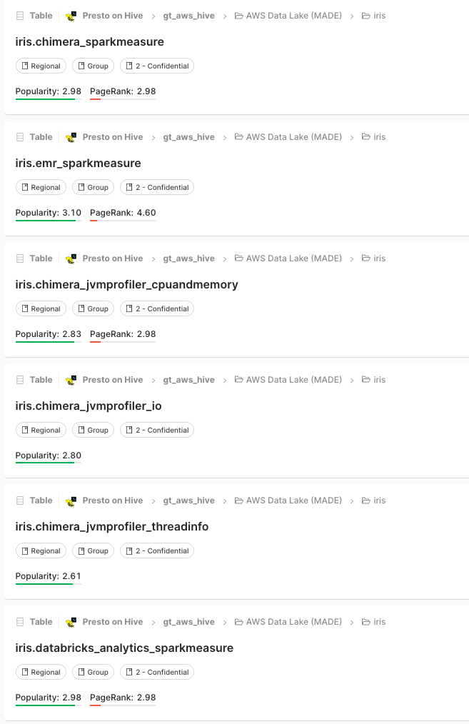
You can now visualize AWS Glue Data Quality scores in data assets that have been published in the Amazon DataZone business catalog and that are searchable through the Amazon DataZone web portal.
If the asset has AWS Glue Data Quality enabled, you can now quickly visualize the data quality score directly in the catalog search pane.

By selecting the corresponding asset, you can understand its content through the readme, glossary terms, and technical and business metadata. Additionally, the overall quality score indicator is displayed in the Asset Details section.

A data quality score serves as an overall indicator of a dataset’s quality, calculated based on the rules you define.
On the Data quality tab, you can access the details of data quality overview indicators and the results of the data quality runs.

The indicators shown on the Overview tab are calculated based on the results of the rulesets from the data quality runs.
Each rule is assigned an attribute that contributes to the calculation of the indicator. For example, rules that have the Completeness attribute will contribute to the calculation of the corresponding indicator on the Overview tab.
To filter data quality results, choose the Applicable column dropdown menu and choose your desired filter parameter.

You can also visualize column-level data quality starting on the Schema tab.

When data quality is enabled for the asset, the data quality results become available, providing insightful quality scores that reflect the integrity and reliability of each column within the dataset.
When you choose one of the data quality result links, you’re redirected to the data quality detail page, filtered by the selected column.

Data quality historical results in Amazon DataZone
Data quality can change over time for many reasons:
- Data formats may change because of changes in the source systems
- As data accumulates over time, it may become outdated or inconsistent
- Data quality can be affected by human errors in data entry, data processing, or data manipulation
In Amazon DataZone, you can now track data quality over time to confirm reliability and accuracy. By analyzing the historical report snapshot, you can identify areas for improvement, implement changes, and measure the effectiveness of those changes.

Enable AWS Glue Data Quality when creating a new Amazon DataZone data source
In this section, we walk through the steps to enable AWS Glue Data Quality when creating a new Amazon DataZone data source.
Prerequisites
To follow along, you should have a domain for Amazon DataZone, an Amazon DataZone project, and a new Amazon DataZone environment (with a DataLakeProfile). For instructions, refer to Amazon DataZone quickstart with AWS Glue data.
You also need to define and run a ruleset against your data, which is a set of data quality rules in AWS Glue Data Quality. To set up the data quality rules and for more information on the topic, refer to the following posts:
After you create the data quality rules, make sure that Amazon DataZone has the permissions to access the AWS Glue database managed through AWS Lake Formation. For instructions, see Configure Lake Formation permissions for Amazon DataZone.
In our example, we have configured a ruleset against a table containing patient data within a healthcare synthetic dataset generated using Synthea. Synthea is a synthetic patient generator that creates realistic patient data and associated medical records that can be used for testing healthcare software applications.
The ruleset contains 27 individual rules (one of them failing), so the overall data quality score is 96%.

If you use Amazon DataZone managed policies, there is no action needed because these will get automatically updated with the needed actions. Otherwise, you need to allow Amazon DataZone to have the required permissions to list and get AWS Glue Data Quality results, as shown in the Amazon DataZone user guide.
Create a data source with data quality enabled
In this section, we create a data source and enable data quality. You can also update an existing data source to enable data quality. We use this data source to import metadata information related to our datasets. Amazon DataZone will also import data quality information related to the (one or more) assets contained in the data source.
- On the Amazon DataZone console, choose Data sources in the navigation pane.
- Choose Create data source.

- For Name, enter a name for your data source.
- For Data source type, select AWS Glue.
- For Environment, choose your environment.
- For Database name, enter a name for the database.
- For Table selection criteria, choose your criteria.
- Choose Next.

- For Data quality, select Enable data quality for this data source.
If data quality is enabled, Amazon DataZone will automatically fetch data quality scores from AWS Glue at each data source run.
- Choose Next.
Now you can run the data source.

While running the data source, Amazon DataZone imports the last 100 AWS Glue Data Quality run results. This information is now visible on the asset page and will be visible to all Amazon DataZone users after publishing the asset.

Enable data quality for an existing data asset
In this section, we enable data quality for an existing asset. This might be useful for users that already have data sources in place and want to enable the feature afterwards.
Prerequisites
To follow along, you should have already run the data source and produced an AWS Glue table data asset. Additionally, you should have defined a ruleset in AWS Glue Data Quality over the target table in the Data Catalog.

For this example, we ran the data quality job multiple times against the table, producing the related AWS Glue Data Quality scores, as shown in the following screenshot.

Import data quality scores into the data asset
Complete the following steps to import the existing AWS Glue Data Quality scores into the data asset in Amazon DataZone:
- Within the Amazon DataZone project, navigate to the Inventory data pane and choose the data source.
If you choose the Data quality tab, you can see that there’s still no information on data quality because AWS Glue Data Quality integration is not enabled for this data asset yet.
- On the Data quality tab, choose Enable data quality.

- In the Data quality section, select Enable data quality for this data source.
- Choose Save.
Now, back on the Inventory data pane, you can see a new tab: Data quality.

On the Data quality tab, you can see data quality scores imported from AWS Glue Data Quality.

Ingest data quality scores from an external source using Amazon DataZone APIs
Many organizations already use systems that calculate data quality by performing tests and assertions on their datasets. Amazon DataZone now supports importing third-party originated data quality scores via API, allowing users that navigate the web portal to view this information.
In this section, we simulate a third-party system pushing data quality scores into Amazon DataZone via APIs through Boto3 (Python SDK for AWS).
For this example, we use the same synthetic dataset as earlier, generated with Synthea.
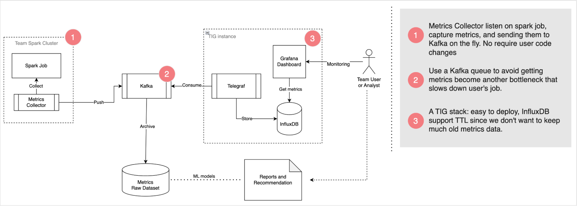
The following diagram illustrates the solution architecture.

The workflow consists of the following steps:
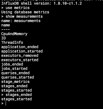
- Read a dataset of patients in Amazon Simple Storage Service (Amazon S3) directly from Amazon EMR using Spark.
The dataset is created as a generic S3 asset collection in Amazon DataZone.
- In Amazon EMR, perform data validation rules against the dataset.
- The metrics are saved in Amazon S3 to have a persistent output.
- Use Amazon DataZone APIs through Boto3 to push custom data quality metadata.
- End-users can see the data quality scores by navigating to the data portal.
Prerequisites
We use Amazon EMR Serverless and Pydeequ to run a fully managed Spark environment. To learn more about Pydeequ as a data testing framework, see Testing Data quality at scale with Pydeequ.
To allow Amazon EMR to send data to the Amazon DataZone domain, make sure that the IAM role used by Amazon EMR has the permissions to do the following:
- Read from and write to the S3 buckets
- Call the
post_time_series_data_points action for Amazon DataZone:
{
    "Version": "2012-10-17",
    "Statement": [
        {
            "Sid": "Statement1",
            "Effect": "Allow",
            "Action": [
                "datazone:PostTimeSeriesDataPoints"
            ],
            "Resource": [
                "<datazone_domain_arn>"
            ]
        }
    ]
}
Make sure that you added the EMR role as a project member in the Amazon DataZone project. On the Amazon DataZone console, navigate to the Project members page and choose Add members.

Add the EMR role as a contributor.

Ingest and analyze PySpark code
In this section, we analyze the PySpark code that we use to perform data quality checks and send the results to Amazon DataZone. You can download the complete PySpark script.
To run the script entirely, you can submit a job to EMR Serverless. The service will take care of scheduling the job and automatically allocating the resources needed, enabling you to track the job run statuses throughout the process.
You can submit a job to EMR within the Amazon EMR console using EMR Studio or programmatically, using the AWS CLI or using one of the AWS SDKs.
In Apache Spark, a SparkSession is the entry point for interacting with DataFrames and Spark’s built-in functions. The script will start initializing a SparkSession:
with SparkSession.builder.appName("PatientsDataValidation") \
        .config("spark.jars.packages", pydeequ.deequ_maven_coord) \
        .config("spark.jars.excludes", pydeequ.f2j_maven_coord) \
        .getOrCreate() as spark:
We read a dataset from Amazon S3. For increased modularity, you can use the script input to refer to the S3 path:
s3inputFilepath = sys.argv[1]
s3outputLocation = sys.argv[2]

df = spark.read.format("csv") \
            .option("header", "true") \
            .option("inferSchema", "true") \
            .load(s3inputFilepath) #s3://<bucket_name>/patients/patients.csv
Next, we set up a metrics repository. This can be helpful to persist the run results in Amazon S3.
metricsRepository = FileSystemMetricsRepository(spark, s3_write_path)
Pydeequ allows you to create data quality rules using the builder pattern, which is a well-known software engineering design pattern, concatenating instruction to instantiate a VerificationSuite object:
key_tags = {'tag': 'patient_df'}
resultKey = ResultKey(spark, ResultKey.current_milli_time(), key_tags)

check = Check(spark, CheckLevel.Error, "Integrity checks")

checkResult = VerificationSuite(spark) \
    .onData(df) \
    .useRepository(metricsRepository) \
    .addCheck(
        check.hasSize(lambda x: x >= 1000) \
        .isComplete("birthdate")  \
        .isUnique("id")  \
        .isComplete("ssn") \
        .isComplete("first") \
        .isComplete("last") \
        .hasMin("healthcare_coverage", lambda x: x == 1000.0)) \
    .saveOrAppendResult(resultKey) \
    .run()

checkResult_df = VerificationResult.checkResultsAsDataFrame(spark, checkResult)
checkResult_df.show()
The following is the output for the data validation rules:
+----------------+-----------+------------+----------------------------------------------------+-----------------+----------------------------------------------------+
|check           |check_level|check_status|constraint                                          |constraint_status|constraint_message                                  |
+----------------+-----------+------------+----------------------------------------------------+-----------------+----------------------------------------------------+
|Integrity checks|Error      |Error       |SizeConstraint(Size(None))                          |Success          |                                                    |
|Integrity checks|Error      |Error       |CompletenessConstraint(Completeness(birthdate,None))|Success          |                                                    |
|Integrity checks|Error      |Error       |UniquenessConstraint(Uniqueness(List(id),None))     |Success          |                                                    |
|Integrity checks|Error      |Error       |CompletenessConstraint(Completeness(ssn,None))      |Success          |                                                    |
|Integrity checks|Error      |Error       |CompletenessConstraint(Completeness(first,None))    |Success          |                                                    |
|Integrity checks|Error      |Error       |CompletenessConstraint(Completeness(last,None))     |Success          |                                                    |
|Integrity checks|Error      |Error       |MinimumConstraint(Minimum(healthcare_coverage,None))|Failure          |Value: 0.0 does not meet the constraint requirement!|
+----------------+-----------+------------+----------------------------------------------------+-----------------+----------------------------------------------------+
At this point, we want to insert these data quality values in Amazon DataZone. To do so, we use the post_time_series_data_points function in the Boto3 Amazon DataZone client.
The PostTimeSeriesDataPoints DataZone API allows you to insert new time series data points for a given asset or listing, without creating a new revision.
At this point, you might also want to have more information on which fields are sent as input for the API. You can use the APIs to obtain the specification for Amazon DataZone form types; in our case, it’s amazon.datazone.DataQualityResultFormType.
You can also use the AWS CLI to invoke the API and display the form structure:
aws datazone get-form-type --domain-identifier <your_domain_id> --form-type-identifier amazon.datazone.DataQualityResultFormType --region <domain_region> --output text --query 'model.smithy'
This output helps identify the required API parameters, including fields and value limits:
$version: "2.0"
namespace amazon.datazone
structure DataQualityResultFormType {
    @amazon.datazone#timeSeriesSummary
    @range(min: 0, max: 100)
    passingPercentage: Double
    @amazon.datazone#timeSeriesSummary
    evaluationsCount: Integer
    evaluations: EvaluationResults
}
@length(min: 0, max: 2000)
list EvaluationResults {
    member: EvaluationResult
}

@length(min: 0, max: 20)
list ApplicableFields {
    member: String
}

@length(min: 0, max: 20)
list EvaluationTypes {
    member: String
}

enum EvaluationStatus {
    PASS,
    FAIL
}

string EvaluationDetailType

map EvaluationDetails {
    key: EvaluationDetailType
    value: String
}

structure EvaluationResult {
    description: String
    types: EvaluationTypes
    applicableFields: ApplicableFields
    status: EvaluationStatus
    details: EvaluationDetails
}
To send the appropriate form data, we need to convert the Pydeequ output to match the DataQualityResultsFormType contract. This can be achieved with a Python function that processes the results.
For each DataFrame row, we extract information from the constraint column. For example, take the following code:
CompletenessConstraint(Completeness(birthdate,None))
We convert it to the following:
{
  "constraint": "CompletenessConstraint",
  "statisticName": "Completeness_custom",
  "column": "birthdate"
}
Make sure to send an output that matches the KPIs that you want to track. In our case, we are appending _custom to the statistic name, resulting in the following format for KPIs:
Completeness_customUniqueness_custom
In a real-world scenario, you might want to set a value that matches with your data quality framework in relation to the KPIs that you want to track in Amazon DataZone.
After applying a transformation function, we have a Python object for each rule evaluation:
..., {
   'applicableFields': ["healthcare_coverage"],
   'types': ["Minimum_custom"],
   'status': 'FAIL',
   'description': 'MinimumConstraint - Minimum - Value: 0.0 does not meet the constraint requirement!'
 },...
We also use the constraint_status column to compute the overall score:
(number of success / total number of evaluation) * 100
In our example, this results in a passing percentage of 85.71%.
We set this value in the passingPercentage input field along with the other information related to the evaluations in the input of the Boto3 method post_time_series_data_points:
import boto3

# Instantiate the client library to communicate with Amazon DataZone Service
#
datazone = boto3.client(
    service_name='datazone',
    region_name=<Region(String) example: us-east-1>
)

# Perform the API operation to push the Data Quality information to Amazon DataZone
#
datazone.post_time_series_data_points(
    domainIdentifier=<DataZone domain ID>,
    entityIdentifier=<DataZone asset ID>,
    entityType='ASSET',
    forms=[
        {
            "content": json.dumps({
                    "evaluationsCount":<Number of evaluations (number)>,
                    "evaluations": [<List of objects {
                        'description': <Description (String)>,
                        'applicableFields': [<List of columns involved (String)>],
                        'types': [<List of KPIs (String)>],
                        'status': <FAIL/PASS (string)>
                        }>
                     ],
                    "passingPercentage":<Score (number)>
                }),
            "formName": <Form name(String) example: PydeequRuleSet1>,
            "typeIdentifier": "amazon.datazone.DataQualityResultFormType",
            "timestamp": <Date (timestamp)>
        }
    ]
)
Boto3 invokes the Amazon DataZone APIs. In these examples, we used Boto3 and Python, but you can choose one of the AWS SDKs developed in the language you prefer.
After setting the appropriate domain and asset ID and running the method, we can check on the Amazon DataZone console that the asset data quality is now visible on the asset page.
We can observe that the overall score matches with the API input value. We can also see that we were able to add customized KPIs on the overview tab through custom types parameter values.
With the new Amazon DataZone APIs, you can load data quality rules from third-party systems into a specific data asset. With this capability, Amazon DataZone allows you to extend the types of indicators present in AWS Glue Data Quality (such as completeness, minimum, and uniqueness) with custom indicators.
Clean up
We recommend deleting any potentially unused resources to avoid incurring unexpected costs. For example, you can delete the Amazon DataZone domain and the EMR application you created during this process.
Conclusion
In this post, we highlighted the latest features of Amazon DataZone for data quality, empowering end-users with enhanced context and visibility into their data assets. Furthermore, we delved into the seamless integration between Amazon DataZone and AWS Glue Data Quality. You can also use the Amazon DataZone APIs to integrate with external data quality providers, enabling you to maintain a comprehensive and robust data strategy within your AWS environment.
To learn more about Amazon DataZone, refer to the Amazon DataZone User Guide.
About the Authors
 Andrea Filippo is a Partner Solutions Architect at AWS supporting Public Sector partners and customers in Italy. He focuses on modern data architectures and helping customers accelerate their cloud journey with serverless technologies.
Emanuele is a Solutions Architect at AWS, based in Italy, after living and working for more than 5 years in Spain. He enjoys helping large companies with the adoption of cloud technologies, and his area of expertise is mainly focused on Data Analytics and Data Management. Outside of work, he enjoys traveling and collecting action figures.
 Varsha Velagapudi is a Senior Technical Product Manager with Amazon DataZone at AWS. She focuses on improving data discovery and curation required for data analytics. She is passionate about simplifying customers’ AI/ML and analytics journey to help them succeed in their day-to-day tasks. Outside of work, she enjoys nature and outdoor activities, reading, and traveling.


 Amir Souchami, Chief Architect of Aura from Unity, focusing on creating resilient and performant cloud systems and mobile apps at major scale.
 Fabian Szenkier is the ML and Big Data Architect at Aura by Unity, works on building modern AI/ML solutions and state of the art data engineering pipelines at scale.
 Liat Tzur is a Senior Technical Account Manager at Amazon Web Services. She serves as the customer’s advocate and assists her customers in achieving cloud operational excellence in alignment with their business goals.
 Adi Jabkowski is a Sr. Redshift Specialist in EMEA, part of the Worldwide Specialist Organization (WWSO) at AWS.
 Yonatan Dolan is a Principal Analytics Specialist at Amazon Web Services. He is located in Israel and helps customers harness AWS analytical services to leverage data, gain insights, and derive value.


 Andrea Filippo is a Partner Solutions Architect at AWS supporting Public Sector partners and customers in Italy. He focuses on modern data architectures and helping customers accelerate their cloud journey with serverless technologies.
 Emanuele is a Solutions Architect at AWS, based in Italy, after living and working for more than 5 years in Spain. He enjoys helping large companies with the adoption of cloud technologies, and his area of expertise is mainly focused on Data Analytics and Data Management. Outside of work, he enjoys traveling and collecting action figures.
 Varsha Velagapudi is a Senior Technical Product Manager with Amazon DataZone at AWS. She focuses on improving data discovery and curation required for data analytics. She is passionate about simplifying customers’ AI/ML and analytics journey to help them succeed in their day-to-day tasks. Outside of work, she enjoys nature and outdoor activities, reading, and traveling.


 Varsha Velagapudi is a Senior Technical Product Manager with Amazon DataZone at AWS. She focuses on improving data discovery and curation required for data analytics. She is passionate about simplifying customers’ AI/ML and analytics journey to help them succeed in their day-to-day tasks. Outside of work, she enjoys playing with her 3-year old, reading, and traveling.
 Zhengyuan Shen is an Applied Scientist at Amazon AWS, specializing in advancements in AI, particularly in large language models and their application in data comprehension. He is passionate about leveraging innovative ML scientific solutions to enhance products or services, thereby simplifying the lives of customers through a seamless blend of science and engineering. Outside of work, he enjoys cooking, weightlifting, and playing poker.
 Balasubramaniam Srinivasan is an Applied Scientist at Amazon AWS, working on foundational models for structured data and natural sciences. He enjoys enriching ML models with domain-specific knowledge and inductive biases to delight customers. Outside of work, he enjoys playing and watching tennis and soccer.


 Ranjit Kalidasan is a Senior Solutions Architect with Amazon Web Services based in Boston, Massachusetts. He is a Partner Solutions Architect helping security ISV partners co-build and co-market solutions with AWS. He brings over 25 years of experience in information technology helping global customers implement complex solutions for security and analytics. You can connect with Ranjit on
  Phaneendra Vuliyaragoli is a Product Management Lead for Amazon Data Firehose at AWS. In this role, Phaneendra leads the product and go-to-market strategy for Amazon Data Firehose.


 Florian Mair is a Senior Solutions Architect and data streaming expert at AWS. He is a technologist that helps customers in Europe succeed and innovate by solving business challenges using AWS Cloud services. Besides working as a Solutions Architect, Florian is a passionate mountaineer, and has climbed some of the highest mountains across Europe.
 Emil Dietl is a Senior Tech Lead at Krones specializing in data engineering, with a key field in Apache Flink and microservices. His work often involves the development and maintenance of mission-critical software. Outside of his professional life, he deeply values spending quality time with his family.
 Simon Peyer is a Solutions Architect at AWS based in Switzerland. He is a practical doer and is passionate about connecting technology and people using AWS Cloud services. A special focus for him is data streaming and automations. Besides work, Simon enjoys his family, the outdoors, and hiking in the mountains.


 Now that you know how to flatten JSON data, you can analyze it further. Use the following query to get the number of minutes a patient has been physically active per day, based on their heart rate (greater than 80):
 Saeed Barghi is a Sr. Analytics Specialist Solutions Architect specializing in architecting enterprise data platforms. He has extensive experience in the fields of data warehousing, data engineering, data lakes, and AI/ML. Based in Melbourne, Australia, Saeed works with public sector customers in Australia and New Zealand.
 Satesh Sonti is a Sr. Analytics Specialist Solutions Architect based out of Atlanta, specialized in building enterprise data platforms, data warehousing, and analytics solutions. He has over 17 years of experience in building data assets and leading complex data platform programs for banking and insurance clients across the globe.


 Ziad WALI is an Acceleration Lab Solutions Architect at Amazon Web Services. He has over 10 years of experience in databases and data warehousing, where he enjoys building reliable, scalable, and efficient solutions. Outside of work, he enjoys sports and spending time in nature.
 Omama Khurshid is an Acceleration Lab Solutions Architect at Amazon Web Services. She focuses on helping customers across various industries build reliable, scalable, and efficient solutions. Outside of work, she enjoys spending time with her family, watching movies, listening to music, and learning new technologies.
 Srikant Das is an Acceleration Lab Solutions Architect at Amazon Web Services. His expertise lies in constructing robust, scalable, and efficient solutions. Beyond the professional sphere, he finds joy in travel and shares his experiences through insightful blogging on social media platforms.


 Ismail Makhlouf is a Senior Specialist Solutions Architect for Data Analytics at AWS. Ismail focuses on architecting solutions for organizations across their end-to-end data analytics estate, including batch and real-time streaming, big data, data warehousing, and data lake workloads. He primarily works with organizations in retail, ecommerce, FinTech, HealthTech, and travel to achieve their business objectives with well architected data platforms.
 Sandipan Bhaumik (Sandi) is a Senior Analytics Specialist Solutions Architect at AWS. He helps customers modernize their data platforms in the cloud to perform analytics securely at scale, reduce operational overhead, and optimize usage for cost-effectiveness and sustainability.


 Ali Alemi is a Streaming Specialist Solutions Architect at AWS. Ali advises AWS customers with architectural best practices and helps them design real-time analytics data systems which are reliable, secure, efficient, and cost-effective. He works backward from customer’s use cases and designs data solutions to solve their business problems. Prior to joining AWS, Ali supported several public sector customers and AWS consulting partners in their application modernization journey and migration to the Cloud.
 Imtiaz (Taz) Sayed is the World-Wide Tech Leader for Analytics at AWS. He enjoys engaging with the community on all things data and analytics. He can be reached via


 Masudur Rahaman Sayem is a Streaming Data Architect at AWS. He works with AWS customers globally to design and build data streaming architectures to solve real-world business problems. He specializes in optimizing solutions that use streaming data services and NoSQL. Sayem is very passionate about distributed computing.
 Michael Oguike is a Product Manager for Amazon MSK. He is passionate about using data to uncover insights that drive action. He enjoys helping customers from a wide range of industries improve their businesses using data streaming. Michael also loves learning about behavioral science and psychology from books and podcasts.


 Jyoti Aggarwal is a Product Management Lead for AWS zero-ETL. She leads the product and business strategy, including driving initiatives around performance, customer experience, and security. She brings along an expertise in cloud compute, data pipelines, analytics, artificial intelligence (AI), and data services including databases, data warehouses and data lakes.
 Sean Beath is an Analytics Solutions Architect at Amazon Web Services. He has experience in the full delivery lifecycle of data platform modernisation using AWS services, and works with customers to help drive analytics value on AWS.
 Gokul Soundararajan is a principal engineer at AWS and received a PhD from University of Toronto and has been working in the areas of storage, databases, and analytics.
 Pratik Patel is Sr. Technical Account Manager and streaming analytics specialist. He works with AWS customers and provides ongoing support and technical guidance to help plan and build solutions using best practices and proactively keep customers’ AWS environments operationally healthy.
 Amar is a Senior Solutions Architect at Amazon AWS in the UK. He works across power, utilities, manufacturing and automotive customers on strategic implementations, specializing in using AWS Streaming and advanced data analytics solutions, to drive optimal business outcomes.


 Sushanth Kothapally is a Solutions Architect at Amazon Web Services supporting Automotive and Manufacturing customers. He is passionate about designing technology solutions to meet business goals and has keen interest in serverless and event-driven architectures.
 Senthil Kamala Rathinam is a Solutions Architect at Amazon Web Services specializing in Data and Analytics. He is passionate about helping customers to design and build modern data platforms. In his free time, Senthil loves to spend time with his family and play badminton.
 Lorenzo Nicora works as Senior Streaming Solution Architect at AWS, helping customers across EMEA. He has been building cloud-native, data-intensive systems for over 25 years, working in the finance industry both through consultancies and for FinTech product companies. He has leveraged open-source technologies extensively and contributed to several projects, including Apache Flink.
 Francisco Morillo is a Streaming Solutions Architect at AWS. Francisco works with AWS customers, helping them design real-time analytics architectures using AWS services, supporting Amazon MSK and Amazon Managed Service for Apache Flink.


 Tony Stricker is a Principal Technologist on the Data Strategy team at AWS, where he helps senior executives adopt a data-driven mindset and align their people/process/technology in ways that foster innovation and drive towards specific, tangible business outcomes. He has a background as a data warehouse architect and data scientist and has delivered solutions in to production across multiple industries including oil and gas, financial services, public sector, and manufacturing. In his spare time, Tony likes to hang out with his dog and cat, work on home improvement projects, and restore vintage Airstream campers.


 Shoukat Ghouse is a Senior Big Data Specialist Solutions Architect at AWS. He helps customers around the world build robust, efficient and scalable data platforms on AWS leveraging AWS analytics services like AWS Glue, AWS Lake Formation, Amazon Athena and Amazon EMR.