Post Syndicated from Lorenzo Nicora original https://aws.amazon.com/blogs/big-data/optimize-checkpointing-in-your-amazon-managed-service-for-apache-flink-applications-with-buffer-debloating-and-unaligned-checkpoints-part-2/
This post is a continuation of a two-part series. In the first part, we delved into Apache Flink‘s internal mechanisms for checkpointing, in-flight data buffering, and handling backpressure. We covered these concepts in order to understand how buffer debloating and unaligned checkpoints allow us to enhance performance for specific conditions in Apache Flink applications.
In Part 1, we introduced and examined how to use buffer debloating to improve in-flight data processing. In this post, we focus on unaligned checkpoints. This feature has been available since Apache Flink 1.11 and has received many improvements since then. Unaligned checkpoints help, under specific conditions, to reduce checkpointing time for applications suffering temporary backpressure, and can be now enabled in Amazon Managed Service for Apache Flink applications running Apache Flink 1.15.2 through a support ticket.
Even though this feature might improve performance for your checkpoints, if your application is constantly failing because of checkpoints timing out, or is suffering from having constant backpressure, you may require a deeper analysis and redesign of your application.
Aligned checkpoints
As discussed in Part 1, Apache Flink checkpointing allows applications to record state in case of failure. We’ve already discussed how checkpoints, when triggered by the job manager, signal all source operators to snapshot their state, which is then broadcasted as a special record called a checkpoint barrier. This process achieves exactly-once consistency for state in a distributed streaming application through the alignment of these barriers.
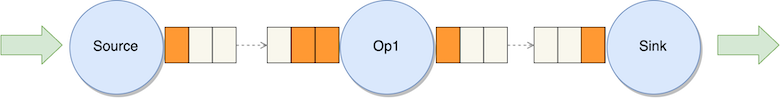
Let’s walk through the process of aligned checkpoints in a standard Apache Flink application. Remember that Apache Flink distributes the workload horizontally: each operator (a node in the logical flow of your application, including sources and sinks) is split into multiple sub-tasks based on its parallelism.
Barrier alignment
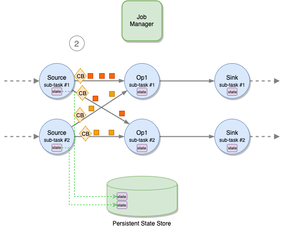
The alignment of checkpoint barriers is crucial for achieving exactly-once consistency in Apache Flink applications during checkpoint runs. To recap, when a job manager triggers a checkpoint, all sub-tasks of source operators receive a signal to initiate the checkpoint process. Each sub-task independently snapshots its state to the state backend and broadcasts a special record known as a checkpoint barrier to all outgoing streams.
When an application operates with a parallelism higher than 1, multiple instances of each task—referred to as sub-tasks—enable parallel message consumption and processing. A sub-task can receive distinct partitions of the same stream from different upstream sub-tasks, such as after a stream repartitioning with keyBy or rebalance operations. To maintain exactly-once consistency, all sub-tasks must wait for the arrival of all checkpoint barriers before taking a snapshot of the state. The following diagram illustrates the checkpoint barriers flow.

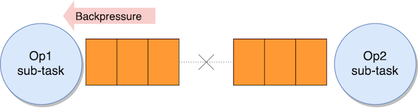
This phase is called checkpoint alignment. During alignment, the sub-task stops processing records from the partitions from which it has already received barriers, as shown in the following figure.

However, it continues to process partitions that are behind the barrier.

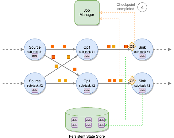
When barriers from all upstream partitions have arrived, the sub-task takes a snapshot of its state.

Then it broadcasts the barrier downstream.

The time a sub-task spends waiting for all barriers to arrive is measured by the checkpoint Alignment Duration metric, which can be observed in the Apache Flink UI.
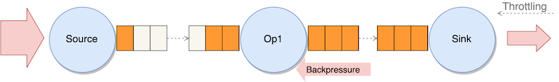
If the application experiences backpressure, an increase in this metric could lead to longer checkpoint durations and even checkpoint failures due to timeouts. This is where unaligned checkpoints become a viable option to potentially enhance checkpointing performance.
Unaligned checkpoints
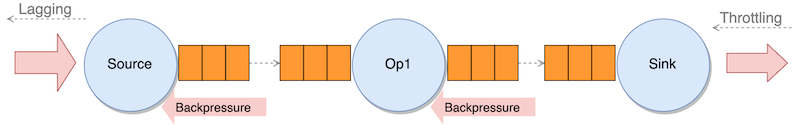
Unaligned checkpoints address situations where backpressure is not just a temporary spike, but results in timeouts for aligned checkpoints, due to barrier queuing within the stream. As discussed in Part 1, checkpoint barriers can’t overtake regular records. Therefore, significant backpressure can slow down the movement of barriers across the application, potentially causing checkpoint timeouts.
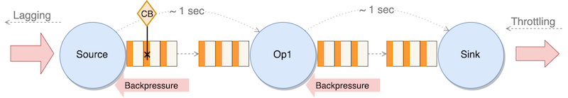
The objective of unaligned checkpoints is to enable barrier overtaking, allowing barriers to move swiftly from source to sink even when the data flow is slower than anticipated.
Building on what we saw in Part 1 concerning checkpoints and what aligned checkpoints are, let’s explore how unaligned checkpoints modify the checkpointing mechanism.
Upon emission, each source’s checkpoint barrier is injected into the stream flowing across sub-tasks. It travels from the source output network buffer queue into the input network buffer queue of the subsequent operator.
Upon the arrival of the first barrier in the input network buffer queue, the operator initially waits for barrier alignment. If the specified alignment timeout expires because not all barriers have reached the end of the input network buffer queue, the operator switches to unaligned checkpoint mode.
The alignment timeout can be set programmatically by env.getCheckpointConfig().setAlignedCheckpointTimeout(Duration.ofSeconds(30)), but modifying the default is not recommended in Apache Flink 1.15.

The operator waits until all checkpoint barriers are present in the input network buffer queue before triggering the checkpoint. Unlike aligned checkpoints, the operator doesn’t need to wait for all barriers to reach the queue’s end, allowing the operator to have in-flight data from the buffer that hasn’t been processed before checkpoint initiation.

After all barriers have arrived in the input network buffer queue, the operator advances the barrier to the end of the output network buffer queue. This enhances checkpointing speed because the barrier can smoothly traverse the application from source to sink, independent of the application’s end-to-end latency.

After forwarding the barrier to the output network buffer queue, the operator initiates the snapshot of in-flight data between the barriers in the input and output network buffer queues, along with the snapshot of the state.
Although processing is momentarily paused during this process, the actual writing to the remote persistent state storage occurs asynchronously, preventing potential bottlenecks.

The local snapshot, encompassing in-flight messages and state, is saved asynchronously in the remote persistent state store, while the barrier continues its journey through the application.

When to use unaligned checkpoints
Remember, barrier alignment only occurs between partitions coming from different sub-tasks of the same operator. Therefore, if an operator is experiencing temporary backpressure, enabling unaligned checkpoints may be beneficial. This way, the application doesn’t have to wait for all barriers to reach the operator before performing the snapshot of state or moving the barrier forward.
Temporary backpressure could arise from the following:
- A surge in data ingestion
- Backfilling or catching up with historical data
- Increased message processing time due to delayed external systems
Another scenario where unaligned checkpoints prove advantageous is when working with exactly-once sinks. Utilizing the two-phase commit sink function for exactly-once sinks, unaligned checkpoints can expedite checkpoint runs, thereby reducing end-to-end latency.
When not to use unaligned checkpoints
Unaligned checkpoints won’t reduce the time required for savepoints (called snapshots in the Amazon Managed Service for Apache Flink implementation) because savepoints exclusively utilize aligned checkpoints. Furthermore, because Apache Flink doesn’t permit concurrent unaligned checkpoints, savepoints won’t occur simultaneously with unaligned checkpoints, potentially elongating savepoint durations.
Unaligned checkpoints won’t fix any underlying issue in your application design. If your application is suffering from persistent backpressure or constant checkpointing timeouts, this might indicate data skewness or underprovisioning, which may require improving and tuning the application.
Using unaligned checkpoints with buffer debloating
One alternative for reducing the risks associated with an increased state size is to combine unaligned checkpoints with buffer debloating. This approach results in having less in-flight data to snapshot and store in the state, along with less data to be used for recovery in case of failure. This synergy facilitates enhanced performance and efficient checkpoint runs, leading to smaller checkpointing sizes and faster recovery times. When testing the use of unaligned checkpoints, we recommend doing so with buffer debloating to prevent the state size from increasing.
Limitations
Unaligned checkpoints are subject to the following limitations:
- They provide no benefit for operators with a parallelism of 1.
- They only improve performance for operators where barrier alignment would have occurred. This alignment happens only if records are coming from different sub-tasks of the same operator, for example, through repartitioning or
keyByoperations. - Operators receiving input from multiple sources or participating in joins might not experience improvements, because the operator would be receiving data from different operators in those cases.
- Although checkpoint barriers can surpass records in the network’s buffer queue, this won’t occur if the sub-task is currently processing a message. If processing a message takes too much time (for example, a flat-map operation emitting numerous records for each input record), barrier handling will be delayed.
- As we have seen, savepoints always use aligned checkpoints. If the savepoints of your applications are slow due to barrier alignment, unaligned checkpoints will not help.
- Additional limitations affect watermarks, message ordering, and broadcast state in recovery. For more details, refer to Limitations.
Considerations
Considerations for implementing unaligned checkpoints:
- Unaligned checkpoints introduce additional I/O to checkpoint storage
- Checkpoints encompass not only operator state but also in-flight data within network buffer queues, leading to increased state size
Recommendations
We offer the following recommendations:
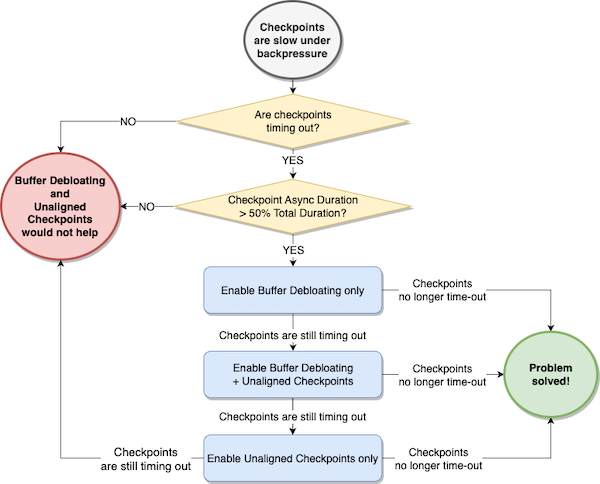
- Consider enabling unaligned checkpoints only if both of the following conditions are true:
- Checkpoints are timing out.
- The average checkpoint Async Duration of any operator is more than 50% of the total checkpoint duration for the operator (sum of Sync Duration + Async Duration).
- Consider enabling buffer debloating first, and evaluate whether it solves the problem of checkpoints timing out.
- If buffer debloating doesn’t help, consider enabling unaligned checkpoints along with buffer debloating. Buffer debloating mitigates the drawbacks of unaligned checkpoints, reducing the amount of in-flight data.
- If unaligned checkpoints and buffer debloating together don’t improve checkpoint alignment duration, consider testing unaligned checkpoints alone.
Finally, but most importantly, always test unaligned checkpoints in a non-production environment first, running some comparative performance testing with a realistic workload, and verify that unaligned checkpoints actually reduce checkpoint duration.
Conclusion
This two-part series explored advanced strategies for optimizing checkpointing within your Amazon Managed Service for Apache Flink applications. By harnessing the potential of buffer debloating and unaligned checkpoints, you can unlock significant performance improvements and streamline checkpoint processes. However, it’s important to understand when these techniques will provide improvements and when they will not. If you believe your application may benefit from checkpoint performance improvement, you can enable these features in your Amazon Managed Service For Apache Flink version 1.15 applications. We recommend first enabling buffer debloating and testing the application. If you are still not seeing the expected outcome, enable buffer debloating with unaligned checkpoints. This way, you can immediately reduce the state size and the additional I/O to state backends. Lastly, you may try using unaligned checkpoints by itself, bearing in mind the considerations we’ve mentioned.
With a deeper understanding of these techniques and their applicability, you are better equipped to maximize the efficiency of checkpoints and mitigate the effect of backpressure in your Apache Flink application.
About the Authors
 Lorenzo Nicora works as Senior Streaming Solution Architect helping customers across EMEA. He has been building cloud-native, data-intensive systems for over 25 years, working in the finance industry both through consultancies and for FinTech product companies. He has leveraged open-source technologies extensively and contributed to several projects, including Apache Flink.
 Francisco Morillo is a Streaming Solutions Architect at AWS. Francisco works with AWS customers helping them design real-time analytics architectures using AWS services, supporting Amazon Managed Streaming for Apache Kafka (Amazon MSK) and AWS’s managed offering for Apache Flink.


 Sushant Majithia is a Principal Product Manager for EMR at AWS.
 Ankur Goyal is a SDM with Amazon EMR Big Data Platform team. He builds large scale distributed applications and cluster optimization algorithms. Ankur is interested in topics of Analytics, Machine Learning and Forecasting.
 Matthew Liem is a Senior Solution Architecture Manager at AWS.
 Tarun Chanana is an SDM with Amazon EMR Big Data Platform team.

 Muthu Pitchaimani is a Search Specialist with Amazon OpenSearch Service. He builds large-scale search applications and solutions. Muthu is interested in the topics of networking and security, and is based out of Austin, Texas.
 Arjun Nambiar is a Product Manager with Amazon OpenSearch Service. He focusses on ingestion technologies that enable ingesting data from a wide variety of sources into Amazon OpenSearch Service at scale. Arjun is interested in large scale distributed systems and cloud-native technologies and is based out of Seattle, Washington.
 Raj Sharma is a Sr. SDM with Amazon OpenSearch Service. He builds large-scale distributed applications and solutions. Raj is interested in the topics of Analytics, databases, networking and security, and is based out of Palo Alto, California.


 Satish Sathiya is a Senior Product Engineer at Amazon Redshift. He is an avid big data enthusiast who collaborates with customers around the globe to achieve success and meet their data warehousing and data lake architecture needs.
 Joshua Luo is a Software Development Engineer for Amazon OpenSearch Serverless. He works on the systems that enable customers to manage and monitor their OpenSearch Serverless resources. He enjoys bouldering, photography, and videography in his free time.
 Satish Nandi is a Senior Technical Product Manager for Amazon OpenSearch Service.


 Ziad WALI is an Acceleration Lab Solutions Architect at Amazon Web Services. He has over 10 years of experience in databases and data warehousing where he enjoys building reliable, scalable and efficient solutions. Outside of work, he enjoys sports and spending time in nature.
 Since we


 Raj Ramasubbu is a Senior Analytics Specialist Solutions Architect focused on big data and analytics and AI/ML with Amazon Web Services. He helps customers architect and build highly scalable, performant, and secure cloud-based solutions on AWS. Raj provided technical expertise and leadership in building data engineering, big data analytics, business intelligence, and data science solutions for over 18 years prior to joining AWS. He helped customers in various industry verticals like healthcare, medical devices, life science, retail, asset management, car insurance, residential REIT, agriculture, title insurance, supply chain, document management, and real estate.


 Aish Gunasekar is a Specialist Solutions architect with a focus on Amazon OpenSearch Service. Her passion at AWS is to help customers design highly scalable architectures and help them in their cloud adoption journey. Outside of work, she enjoys hiking and baking.
 Jimish Shah is a Senior Product Manager at AWS with 15+ years of experience bringing products to market in log analytics, cybersecurity, and IP video streaming. He’s passionate about launching products that offer delightful customer experiences, and solve complex customer problems. In his free time, he enjoys exploring cafes, hiking, and taking long walks.


 Anand Komandooru is a Senior Cloud Architect at AWS. He joined AWS Professional Services organization in 2021 and helps customers build cloud-native applications on AWS cloud. He has over 20 years of experience building software and his favorite Amazon leadership principle is “
 Li Liu is a Senior Database Specialty Architect with the Professional Services team at Amazon Web Services. She helps customers migrate traditional on-premise databases to the AWS Cloud. She specializes in database design, architecture, and performance tuning.
 Neil Potter is a Senior Cloud Application Architect at AWS. He works with AWS customers to help them migrate their workloads to the AWS Cloud. He specializes in application modernization and cloud-native design and is based in New Jersey.
 Vivek Shrivastava is a Principal Data Architect, Data Lake in AWS Professional Services. He is a big data enthusiast and holds 14 AWS Certifications. He is passionate about helping customers build scalable and high-performance data analytics solutions in the cloud. In his spare time, he loves reading and finds areas for home automation.
 Stavros Macrakis is a Senior Technical Product Manager on the OpenSearch project of Amazon Web Services. He is passionate about giving customers the tools to improve the quality of their search results.


 Sandeep Adwankar is a Senior Technical Product Manager at AWS. Based in the California Bay Area, he works with customers around the globe to translate business and technical requirements into products that enable customers to improve how they manage, secure, and access data.
 Srividya Parthasarathy is a Senior Big Data Architect on the AWS Lake Formation team. She enjoys building data mesh solutions and sharing them with the community.
 Mahesh Mishra is a Principal Product Manager with AWS Lake Formation team. He works with many of AWS largest customers on emerging technology needs, and leads several data and analytics initiatives within AWS including strong support for Transactional Data Lakes.


 Vijay Velpula is a Data Lake Architect with AWS Professional Services. He helps customers building modern data platforms through implementing Big Data & Analytics solutions. Outside of work, he enjoys spending time with family, traveling, hiking and biking.
 Karthikeyan Ramachandran is a Data Architect with AWS Professional Services. He specializes in MPP systems helping Customers build and maintain Data warehouse environments. Outside of work, he likes to binge-watch tv shows and loves playing cricket and volleyball.
 Sriharsh Adari is a Senior Solutions Architect at Amazon Web Services (AWS), where he helps customers work backwards from business outcomes to develop innovative solutions on AWS. Over the years, he has helped multiple customers on data platform transformations across industry verticals. His core area of expertise include Technology Strategy, Data Analytics, and Data Science. In his spare time, he enjoys playing sports, binge-watching TV shows, and playing Tabla.


 Aparajithan Vaidyanathan is a Principal Enterprise Solutions Architect at AWS. He supports enterprise customers migrate and modernize their workloads on AWS cloud. He is a Cloud Architect with 23+ years of experience designing and developing enterprise, large-scale and distributed software systems. He specializes in Machine Learning & Data Analytics with focus on Data and Feature Engineering domain. He is an aspiring marathon runner and his hobbies include hiking, bike riding and spending time with his wife and two boys.
 Hafiz Saadullah is a Principal Technical Product Manager at Amazon Web Services. Hafiz focuses on AWS Solutions, designed to help customers by addressing common business problems and use cases.


 Jonathan Wong is a Solutions Architect at AWS assisting with initiatives within Strategic Accounts. He is passionate about solving customer challenges and has been exploring emerging technologies to accelerate innovation.


 Prashant Agrawal is a Sr. Search Specialist Solutions Architect with Amazon OpenSearch Service. He works closely with customers to help them migrate their workloads to the cloud and helps existing customers fine-tune their clusters to achieve better performance and save on cost. Before joining AWS, he helped various customers use OpenSearch and Elasticsearch for their search and log analytics use cases. When not working, you can find him traveling and exploring new places. In short, he likes doing Eat → Travel → Repeat.


 Aarthi Srinivasan is a Senior Big Data Architect with AWS Lake Formation. She likes building data lake solutions for AWS customers and partners. When not on the keyboard, she explores the latest science and technology trends and spends time with her family.


 Thomas Burns,
  Aileen Zheng is a Solutions Architect supporting US Federal Civilian Sciences customers at Amazon Web Services (AWS). She partners with customers to provide technical guidance on enterprise cloud adoption and strategy and helps with building well-architected solutions. She is also very passionate about data analytics and machine learning. In her free time, you’ll find Aileen doing pilates, taking her dog Mumu out for a hike, or hunting down another good spot for food! You’ll also see her contributing to projects to support diversity and women in technology.