Post Syndicated from Gonzalo Herreros original https://aws.amazon.com/blogs/big-data/best-practices-to-optimize-cost-and-performance-for-aws-glue-streaming-etl-jobs/
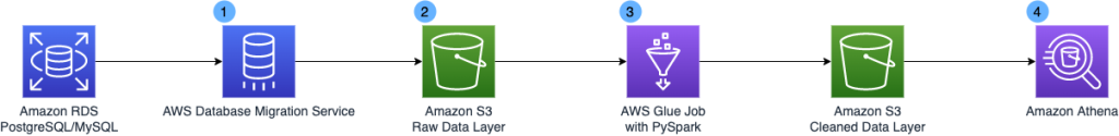
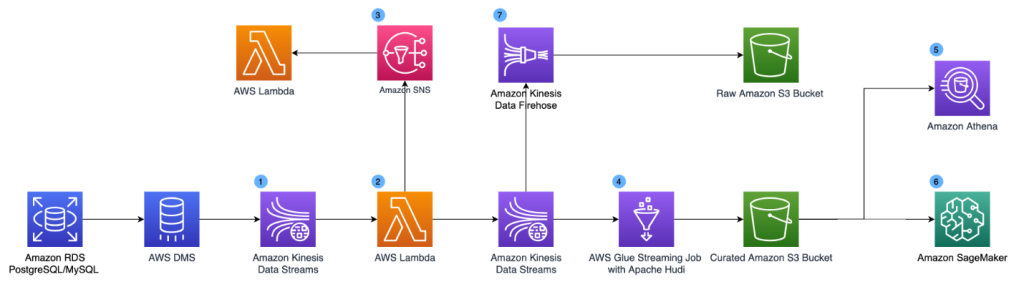
AWS Glue streaming extract, transform, and load (ETL) jobs allow you to process and enrich vast amounts of incoming data from systems such as Amazon Kinesis Data Streams, Amazon Managed Streaming for Apache Kafka (Amazon MSK), or any other Apache Kafka cluster. It uses the Spark Structured Streaming framework to perform data processing in near-real time.
This post covers use cases where data needs to be efficiently processed, delivered, and possibly actioned in a limited amount of time. This can cover a wide range of cases, such as log processing and alarming, continuous data ingestion and enrichment, data validation, internet of things, machine learning (ML), and more.
We discuss the following topics:
- Development tools that help you code faster using our newly launched AWS Glue Studio notebooks
- How to monitor and tune your streaming jobs
- Best practices for sizing and scaling your AWS Glue cluster, using our newly launched features like auto scaling and the small worker type G 0.25X
Development tools
AWS Glue Studio notebooks can speed up the development of your streaming job by allowing data engineers to work using an interactive notebook and test code changes to get quick feedback—from business logic coding to testing configuration changes—as part of tuning.
Before you run any code in the notebook (which would start the session), you need to set some important configurations.
The magic %streaming creates the session cluster using the same runtime as AWS Glue streaming jobs. This way, you interactively develop and test your code using the same runtime that you use later in the production job.
Additionally, configure Spark UI logs, which will be very useful for monitoring and tuning the job.
See the following configuration:
%streaming
%%configure
{
"--enable-spark-ui": "true",
"--spark-event-logs-path": "s3://your_bucket/sparkui/"
}
For additional configuration options such as version or number of workers, refer to Configuring AWS Glue interactive sessions for Jupyter and AWS Glue Studio notebooks.
To visualize the Spark UI logs, you need a Spark history server. If you don’t have one already, refer to Launching the Spark History Server for deployment instructions.
Structured Streaming is based on streaming DataFrames, which represent micro-batches of messages.
The following code is an example of creating a stream DataFrame using Amazon Kinesis as the source:
kinesis_options = {
  "streamARN": "arn:aws:kinesis:us-east-2:777788889999:stream/fromOptionsStream",
  "startingPosition": "TRIM_HORIZON",
  "inferSchema": "true",
  "classification": "json"
}
kinesisDF = glueContext.create_data_frame_from_options(
   connection_type="kinesis",
   connection_options=kinesis_options
)
The AWS Glue API helps you create the DataFrame by doing schema detection and auto decompression, depending on the format. You can also build it yourself using the Spark API directly:
kinesisDF = spark.readStream.format("kinesis").options(**kinesis_options).load()
After your run any code cell, it triggers the startup of the session, and the application soon appears in the history server as an incomplete app (at the bottom of the page there is a link to display incomplete apps) named GlueReplApp, because it’s a session cluster. For a regular job, it’s listed with the job name given when it was created.

From the notebook, you can take a sample of the streaming data. This can help development and give an indication of the type and size of the streaming messages, which might impact performance.
Monitor the cluster with Structured Streaming
The best way to monitor and tune your AWS Glue streaming job is using the Spark UI; it gives you the overall streaming job trends on the Structured Streaming tab and the details of each individual micro-batch processing job.
Overall view of the streaming job
On the Structured Streaming tab, you can see a summary of the streams running in the cluster, as in the following example.

Normally there is just one streaming query, representing a streaming ETL. If you start multiple in parallel, it’s good if you give it a recognizable name, calling queryName() if you use the writeStream API directly on the DataFrame.
After a good number of batches are complete (such as 10), enough for the averages to stabilize, you can use Avg Input/sec column to monitor how many events or messages the job is processing. This can be confusing because the column to the right, Avg Process/sec, is similar but often has a higher number. The difference is that this process time tells us how efficient our code is, whereas the average input tells us how many messages the cluster is reading and processing.
The important thing to note is that if the two values are similar, it means the job is working at maximum capacity. It’s making the best use of the hardware but it likely won’t be able to cope with an increase in volume without causing delays.
In the last column is the latest batch number. Because they’re numbered incrementally from zero, this tells us how many batches the query has processed so far.
When you choose the link in the “Run ID” column of a streaming query, you can review the details with graphs and histograms, as in the following example.

The first two rows correspond to the data that is used to calculate the averages shown on the summary page.
For Input Rate, each data point is calculated by dividing the number of events read for the batch by the time passed between the current batch start and the previous batch start. In a healthy system that is able to keep up, this is equal to the configured trigger interval (in the GlueContext.forEachBatch() API, this is set using the option windowSize).
Because it uses the current batch rows with the previous batch latency, this graph is often unstable in the first batches until the Batch Duration (the last line graph) stabilizes.
In this example, when it stabilizes, it gets completely flat. This means that either the influx of messages is constant or the job is hitting the limit per batch set (we discuss how to do this later in the post).
Be careful if you set a limit per batch that is constantly hit, you could be silently building a backlog, but everything could look good in the job metrics. To monitor this, have a metric of latency measuring the difference between the message timestamp when it gets created and the time it’s processed.
Process Rate is calculated by dividing the number of messages in a batch by the time it took to process that batch. For instance, if the batch contains 1,000 messages, and the trigger interval is 10 seconds but the batch only needed 5 seconds to process it, the process rate would be 1000/5 = 200 msg/sec. while the input rate for that batch (assuming the previous batch also ran within the interval) is 1000/10 = 100 msg/sec.
This metric is useful to measure how efficient our code processing the batch is, and therefore it can get higher than the input rate (this doesn’t mean it’s processing more messages, just using less time). As mentioned earlier, if both metrics get close, it means the batch duration is close to the interval and therefore additional traffic is likely to start causing batch trigger delays (because the previous batch is still running) and increase latency.
Later in this post, we show how auto scaling can help prevent this situation.
Input Rows shows the number of messages read for each batch, like input rate, but using volume instead of rate.
It’s important to note that if the batch processes the data multiple times (for example, writing to multiple destinations), the messages are counted multiple times. If the rates are greater than the expected, this could be the reason. In general, to avoid reading messages multiple times, you should cache the batch while processing it, which is the default when you use the GlueContext.forEachBatch() API.
The last two rows tell us how long it takes to process each batch and how is that time spent. It’s normal to see the first batches take much longer until the system warms up and stabilizes.
The important thing to look for is that the durations are roughly stable and well under the configured trigger interval. If that’s not the case, the next batch gets delayed and could start a compounding delay by building a backlog or increasing batch size (if the limit allows taking the extra messages pending).
In Operation Duration, the majority of time should be spent on addBatch (the mustard color), which is the actual work. The rest are fixed overhead, therefore the smaller the batch process, the more percentage of time that will take. This represents the trade-off between small batches with lower latency or bigger batches but more computing efficient.
Also, it’s normal for the first batch to spend significant time in the latestOffset (the brown bar), locating the point at which it needs to start processing when there is no checkpoint.
The following query statistics show another example.

In this case, the input has some variation (meaning it’s not hitting the batch limit). Also, the process rate is roughly the same as the input rate. This tells us the system is at max capacity and struggling to keep up. By comparing the input rows and input rate, we can guess that the interval configured is just 3 seconds and the batch duration is barely able to meet that latency.
Finally, in Operation Duration, you can observe that because the batches are so frequent, a significant amount of time (proportionally speaking) is spent saving the checkpoint (the dark green bar).
With this information, we can probably improve the stability of the job by increasing the trigger interval to 5 seconds or more. This way, it checkpoints less often and has more time to process data, which might be enough to get batch duration consistently under the interval. The trade-off is that the latency between when a message is published and when it’s processed is longer.
Monitor individual batch processing
On the Jobs tab, you can see how long each batch is taking and dig into the different steps the processing involves to understand how the time is spent. You can also check if there are tasks that succeed after retry. If this happens continuously, it can silently hurt performance.
For instance, the following screenshot shows the batches on the Jobs tab of the Spark UI of our streaming job.

Each batch is considered a job by Spark (don’t confuse the job ID with the batch number; they only match if there is no other action). The job group is the streaming query ID (this is important only when running multiple queries).
The streaming job in this example has a single stage with 100 partitions. Both batches processed them successfully, so the stage is marked as succeeded and all the tasks completed (100/100 in the progress bar).
However, there is a difference in the first batch: there were 20 task failures. You know all the failed tasks succeeded in the retries, otherwise the stage would have been marked as failed. For the stage to fail, the same task would have to fail four times (or as configured by spark.task.maxFailures).
If the stage fails, the batch fails as well and possibly the whole job; if the job was started by using GlueContext.forEachBatch(), it has a number of retries as per the batchMaxRetries parameter (three by default).
These failures are important because they have two effects:
- They can silently cause delays in the batch processing, depending on how long it took to fail and retry.
- They can cause records to be sent multiple times if the failure is in the last stage of the batch, depending on the type of output. If the output is files, in general it won’t cause duplicates. However, if the destination is Amazon DynamoDB, JDBC, Amazon OpenSearch Service, or another output that uses batching, it’s possible that some part of the output has already been sent. If you can’t tolerate any duplicates, the destination system should handle this (for example, being idempotent).
Choosing the description link takes you to the Stages tab for that job. Here you can dig into the failure: What is the exception? Is it always in the same executor? Does it succeed on the first retry or took multiple?
Ideally, you want to identify these failures and solve them. For example, maybe the destination system is throttling us because doesn’t have enough provisioned capacity, or a larger timeout is needed. Otherwise, you should at least monitor it and decide if it is systemic or sporadic.
Sizing and scaling
Defining how to split the data is a key element in any distributed system to run and scale efficiently. The design decisions on the messaging system will have a strong influence on how the streaming job will perform and scale, and thereby affect the job parallelism.
In the case of AWS Glue Streaming, this division of work is based on Apache Spark partitions, which define how to split the work so it can be processed in parallel. Each time the job reads a batch from the source, it divides the incoming data into Spark partitions.
For Apache Kafka, each topic partition becomes a Spark partition; similarly, for Kinesis, each stream shard becomes a Spark partition. To simplify, I’ll refer to this parallelism level as number of partitions, meaning Spark partitions that will be determined by the input Kafka partitions or Kinesis shards on a one-to-one basis.
The goal is to have enough parallelism and capacity to process each batch of data in less time than the configured batch interval and therefore be able to keep up. For instance, with a batch interval of 60 seconds, the job lets 60 seconds of data build up and then processes that data. If that work takes more than 60 seconds, the next batch waits until the previous batch is complete before starting a new batch with the data that has built up since the previous batch started.
It’s a good practice to limit the amount of data to process in a single batch, instead of just taking everything that has been added since the last one. This helps make the job more stable and predictable during peak times. It allows you to test that the job can handle volume of data without issues (for example, memory or throttling).
To do so, specify a limit when defining the source stream DataFrame:
- For Kinesis, specify the limit using
kinesis.executor.maxFetchRecordsPerShard, and revise this number if the number of shards changes substantially. You might need to increase kinesis.executor.maxFetchTimeInMs as well, in order to allow more time to read the batch and make sure it’s not truncated.
- For Kafka, set
maxOffsetsPerTrigger, which divides that allowance equally between the number of partitions.
The following is an example of setting this config for Kafka (for Kinesis, it’s equivalent but using Kinesis properties):
kafka_properties= {
  "kafka.bootstrap.servers": "bootstrapserver1:9092",
  "subscribe": "mytopic",
  "startingOffsets": "latest",
  "maxOffsetsPerTrigger": "5000000"
}
# Pass the properties as options when creating the DataFrame
spark.spark.readStream.format("kafka").options(**kafka_properties).load()
Initial benchmark
If the events can be processed individually (no interdependency such as grouping), you can get a rough estimation of how many messages a single Spark core can handle by running with a single partition source (one Kafka partition or one Kinesis shard stream) with data preloaded into it and run batches with a limit and the minimum interval (1 second). This simulates a stress test with no downtime between batches.
For these repeated tests, clear the checkpoint directory, use a different one (for example, make it dynamic using the timestamp in the path), or just disable the checkpointing (if using the Spark API directly), so you can reuse the same data.
Leave a few batches to run (at least 10) to give time for the system and the metrics to stabilize.
Start with a small limit (using the limit configuration properties explained in the previous section) and do multiple reruns, increasing the value. Record the batch duration for that limit and the throughput input rate (because it’s a stress test, the process rate should be similar).
In general, larger batches tend to be more efficient up to a point. This is because the fixed overhead taken for each to checkpoint, plan, and coordinate the nodes is more significant if the batches are smaller and therefore more frequent.
Then pick your reference initial settings based on the requirements:
- If a goal SLA is required, use the largest batch size whose batch duration is less than half the latency SLA. This is because in the worst case, a message that is stored just after a batch is triggered has to wait at least the interval and then the processing time (which should be less than the interval). When the system is keeping up, the latency in this worst case would be close to twice the interval, so aim for the batch duration to be less than half the target latency.
- In the case where the throughput is the priority over latency, just pick the batch size that provides a higher average process rate and define an interval that allows some buffer over the observed batch duration.
Now you have an idea of the number of messages per core our ETL can handle and the latency. These numbers are idealistic because the system won’t scale perfectly linearly when you add more partitions and nodes. You can use the messages per core obtained to divide the total number of messages per second to process and get the minimum number of Spark partitions needed (each core handles one partition in parallel).
With this number of estimated Spark cores, calculate the number of nodes needed depending on the type and version, as summarized in the following table.
| AWS Glue Version |
Worker Type |
vCores |
Spark Cores per Worker |
| 2 |
G 1X |
4 |
8 |
| 2 |
G 2X |
8 |
16 |
| 3 |
G 0.25X |
2 |
2 |
| 3 |
G 1X |
4 |
4 |
| 3 |
G 2X |
8 |
8 |
Using the newer version 3 is preferable because it includes more optimizations and features like auto scaling (which we discuss later). Regarding size, unless the job has some operation that is heavy on memory, it’s preferable to use the smaller instances so there aren’t so many cores competing for memory, disk, and network shared resources.
Spark cores are equivalent to threads; therefore, you can have more (or less) than the actual cores available in the instance. This doesn’t mean that having more Spark cores is going to necessarily be faster if they’re not backed by physical cores, it just means you have more parallelism competing for the same CPU.
Sizing the cluster when you control the input message system
This is the ideal case because you can optimize the performance and the efficiency as needed.
With the benchmark information you just gathered, you can define your initial AWS Glue cluster size and configure Kafka or Kinesis with the number of partitions or topics estimated, plus some buffer. Test this baseline setup and adjust as needed until the job can comfortably meet the total volume and required latency.
For instance, if we have determined that we need 32 cores to be well within the latency requirement for the volume of data to process, then we can create an AWS Glue 3.0 cluster with 9 G.1X nodes (a driver and 8 workers with 4 cores = 32) which reads from a Kinesis data stream with 32 shards.
Imagine that the volume of data in that stream doubles and we want to keep the latency requirements. To do so, we double the number of workers (16 + 1 driver = 17) and the number of shards on the stream (now 64). Remember this is just a reference and needs to be validated; in practice you might need more or less nodes depending on the cluster size, if the destination system can keep up, complexity of transformations, or other parameters.
Sizing the cluster when you don’t control the message system configuration
In this case, your options for tuning are much more limited.
Check if a cluster with the same number of Spark cores as existing partitions (determined by the message system) is able to keep up with the expected volume of data and latency, plus some allowance for peak times.
If that’s not the case, adding more nodes alone won’t help. You need to repartition the incoming data inside AWS Glue. This operation adds an overhead to redistribute the data internally, but it’s the only way the job can scale out in this scenario.
Let’s illustrate with an example. Imagine we have a Kinesis data stream with one shard that we don’t control, and there isn’t enough volume to justify asking the owner to increase the shards. In the cluster, significant computing for each message is needed; for each message, it runs heuristics and other ML techniques to take action depending on the calculations. After running some benchmarks, the calculations can be done promptly for the expected volume of messages using 8 cores working in parallel. By default, because there is only one shard, only one core will process all the messages sequentially.
To solve this scenario, we can provision an AWS Glue 3.0 cluster with 3 G 1X nodes to have 8 worker cores available. In the code repartition, the batch distributes the messages randomly (as evenly as possible) between them:
def batch_function(data_frame, batch_id):
    # Repartition so the udf is called in parallel for each partition
    data_frame.repartition(8).foreach(process_event_udf)

glueContext.forEachBatch(frame=streaming_df, batch_function=batch_function)
If the messaging system resizes the number of partitions or shards, the job picks up this change on the next batch. You might need to adjust the cluster capacity accordingly with the new data volume.
The streaming job is able to process more partitions than Spark cores are available, but might cause inefficiencies because the additional partitions will be queued and won’t start being processed until others finish. This might result in many nodes being idle while the remaining partitions finish and the next batch can be triggered.
When the messages have processing interdependencies
If the messages to be processed depend on other messages (either in the same or previous batches), that’s likely to be a limiting factor on the scalability. In that case, it might help to analyze a batch (job in Spark UI) to see where the time is spent and if there are imbalances by checking the task duration percentiles on the Stages tab (you can also reach this page by choosing a stage on the Jobs tab).
Auto scaling
Up to now, you have seen sizing methods to handle a stable stream of data with the occasional peak.
However, for variable incoming volumes of data, this isn’t cost-effective because you need to size for the worst-case scenario or accept higher latency at peak times.
This is where AWS Glue Streaming 3.0 auto scaling comes in. You can enable it for the job and define the maximum number of workers you want to allow (for example, using the number you have determined needed for the peak times).
The runtime monitors the trend of time spent on batch processing and compares it with the configured interval. Based on that, it makes a decision to increase or decrease the number of workers as needed, being more aggressive as the batch times get near or go over the allowed interval time.
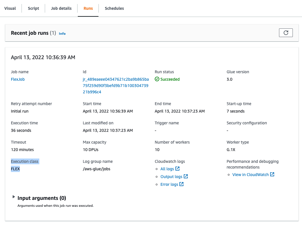
The following screenshot is an example of a streaming job with auto scaling enabled.

Splitting workloads
You have seen how to scale a single job by adding nodes and partitioning the data as needed, which is enough on most cases. As the cluster grows, there is still a single driver and the nodes have to wait for the others to complete the batch before they can take additional work. If it reaches a point that increasing the cluster size is no longer effective, you might want to consider splitting the workload between separate jobs.
In the case of Kinesis, you need to divide the data into multiple streams, but for Apache Kafka, you can divide a topic into multiple jobs by assigning partitions to each one. To do so, instead of the usual subscribe or subscribePattern where the topics are listed, use the property assign to assign using JSON a subset of the topic partitions that the job will handle (for example, {"topic1": [0,1,2]}). At the time of this writing, it’s not possible to specify a range, so you need to list all the partitions, for instance building that list dynamically in the code.
Sizing down
For low volumes of traffic, AWS Glue Streaming has a special type of small node: G 0.25X, which provides two cores and 4 GB RAM for a quarter of the cost of a DPU, so it’s very cost-effective. However, even with that frugal capacity, if you have many small streams, having a small cluster for each one is still not practical.
For such situations, there are currently a few options:
- Configure the stream DataFrame to feed from multiple Kafka topics or Kinesis streams. Then in the DataFrame, use the columns
topic and streamName, for Kafka and Kinesis sources respectively, to determine how to handle the data (for example, different transformations or destinations). Make sure the DataFrame is cached, so you don’t read the data multiple times.
- If you have a mix of Kafka and Kinesis sources, you can define a DataFrame for each, join them, and process as needed using the columns mentioned in the previous point.
- The preceding two cases require all the sources to have the same batch interval and links their processing (for example, a busier stream can delay a slower one). To have independent stream processing inside the same cluster, you can trigger the processing of separate stream’s DataFrames using separate threads. Each stream is monitored separately in the Spark UI, but you’re responsible for starting and managing those threads and handle errors.
Settings
In this post, we showed some config settings that impact performance. The following table summarizes the ones we discussed and other important config properties to use when creating the input stream DataFrame.
| Property |
Applies to |
Remarks |
maxOffsetsPerTrigger |
Kafka |
Limit of messages per batch. Divides the limit evenly among partitions. |
kinesis.executor.maxFetchRecordsPerShard |
Kinesis |
Limit per each shard, therefore should be revised if the number of shards changes. |
kinesis.executor.maxFetchTimeInMs |
Kinesis |
When increasing the batch size (either by increasing the batch interval or the previous property), the executor might need more time, allotted by this property. |
startingOffsets |
Kafka |
Normally you want to read all the data available and therefore use earliest. However, if there is a big backlog, the system might take a long time to catch up and instead use latest to skip the history. |
startingposition |
Kinesis |
Similar to startingOffsets, in this case the values to use are TRIM_HORIZON to backload and LATEST to start processing from now on. |
includeHeaders |
Kafka |
Enable this flag if you need to merge and split multiple topics in the same job (see the previous section for details). |
kinesis.executor.maxconnections |
Kinesis |
When writing to Kinesis, by default it uses a single connection. Increasing this might improve performance. |
kinesis.client.avoidEmptyBatches |
Kinesis |
It’s best to set it to true to avoid wasting resources (for example, generating empty files) when there is no data (like the Kafka connector does). GlueContext.forEachBatch prevents empty batches by default. |
Further optimizations
In general, it’s worth doing some compression on the messages to save on transfer time (at the expense of some CPU, depending on the compression type used).
If the producer compresses the messages individually, AWS Glue can detect it and decompress automatically in most cases, depending on the format and type. For more information, refer to Adding Streaming ETL Jobs in AWS Glue.
If using Kafka, you have the option to compress the topic. This way, the compression is more effective because it’s done in batches, end-to-end, and it’s transparent to the producer and consumer.
By default, the GlueContext.forEachBatch function caches the incoming data. This is helpful if the data needs to be sent to multiple sinks (for example, as Amazon S3 files and also to update a DynamoDB table) because otherwise the job would read the data multiple times from the source. But it can be detrimental to performance if the volume of data is big and there is only one output.
To disable this option, set persistDataFrame as false:
glueContext.forEachBatch(
    frame=myStreamDataFrame,
    batch_function=processBatch,
    options={
        "windowSize": "30 seconds",
        "checkpointLocation": myCheckpointPath,
        "persistDataFrame":  "false"
    }
)
In streaming jobs, it’s common to have to join streaming data with another DataFrame to do enrichment (for example, lookups). In that case, you want to avoid any shuffle if possible, because it splits stages and causes data to be moved between nodes.
When the DataFrame you’re joining to is relatively small to fit in memory, consider using a broadcast join. However, bear in mind it will be distributed to the nodes on every batch, so it might not be worth it if the batches are too small.
If you need to shuffle, consider enabling the Kryo serializer (if using custom serializable classes you need to register them first to use it).
As in any AWS Glue jobs, avoid using custom udf() if you can do the same with the provided API like Spark SQL. User-defined functions (UDFs) prevent the runtime engine from performing many optimizations (the UDF code is a black box for the engine) and in the case of Python, it forces the movement of data between processes.
Avoid generating too many small files (especially columnar like Parquet or ORC, which have overhead per file). To do so, it might be a good idea to coalesce the micro-batch DataFrame before writing the output. If you’re writing partitioned data to Amazon S3, repartition based on columns can significantly reduce the number of output files created.
Conclusion
In this post, you saw how to approach sizing and tuning an AWS Glue streaming job in different scenarios, including planning considerations, configuration, monitoring, tips, and pitfalls.
You can now use these techniques to monitor and improve your existing streaming jobs or use them when designing and building new ones.
About the author
 Gonzalo Herreros is a Senior Big Data Architect on the AWS Glue team.

 Kevin Chun is a Staff Software Engineer in Core Engineering at NerdWallet. He builds data infrastructure and tooling to help NerdWallet provide clarity for all of life’s financial decisions.
 Dylan Qu is a Specialist Solutions Architect focused on big data and analytics with Amazon Web Services. He helps customers architect and build highly scalable, performant, and secure cloud-based solutions on AWS.
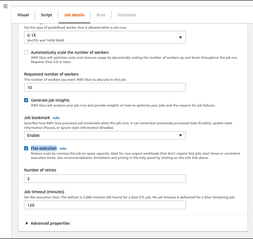


 Dhiraj Thakur is a Solutions Architect with Amazon Web Services. He works with AWS customers and partners to provide guidance on enterprise cloud adoption, migration, and strategy. He is passionate about technology and enjoys building and experimenting in the analytics and AI/ML space.


 Varad Ram is Senior Solutions Architect in Amazon Web Services. He likes to help customers adopt to cloud technologies and is particularly interested in artificial intelligence. He believes deep learning will power future technology growth. In his spare time, he like to be outdoor with his daughter and son.