Post Syndicated from Moustafa Mahmoud original https://aws.amazon.com/blogs/big-data/land-data-from-databases-to-a-data-lake-at-scale-using-aws-glue-blueprints/
To build a data lake on AWS, a common data ingestion pattern is to use AWS Glue jobs to perform extract, transform, and load (ETL) data from relational databases to Amazon Simple Storage Service (Amazon S3). A project often involves extracting hundreds of tables from source databases to the data lake raw layer. And for each source table, it’s recommended to have a separate AWS Glue job to simplify operations, state management, and error handling. This approach works perfectly with a small number of tables. However, with hundreds of tables, this results in hundreds of ETL jobs, and managing AWS Glue jobs at this scale may pose an operational challenge if you’re not yet ready to deploy using a CI/CD pipeline. Instead, we tackle this issue by decoupling the following:
- ETL job logic – We use an AWS Glue blueprint, which allows you to reuse one blueprint for all jobs with the same logic
- Job definition – We use a JSON file, so you can define jobs programmatically without learning a new language
- Job deployment – With AWS Step Functions, you can copy workflows to manage different data processing use cases on AWS Glue
In this post, you will learn how to handle data lake landing jobs deployment in a standardized way—by maintaining a JSON file with table names and a few parameters (for example, a workflow catalog). AWS Glue workflows are created and updated after manually running the resources deployment flow in Step Functions. You can further customize the AWS Glue blueprints to make your own multi-step data pipelines to move data to downstream layers and purpose-built analytics services (example use cases include partitioning or importing to an Amazon DynamoDB table).
Overview of solution
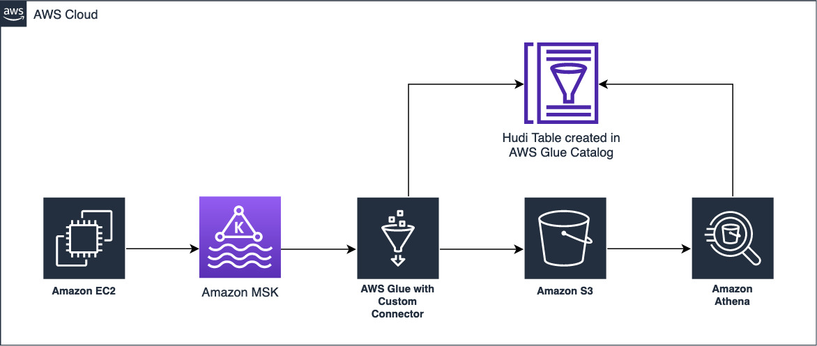
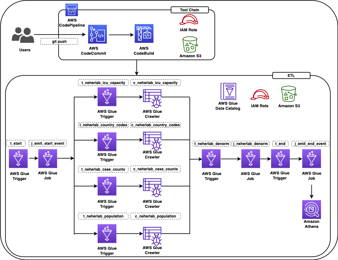
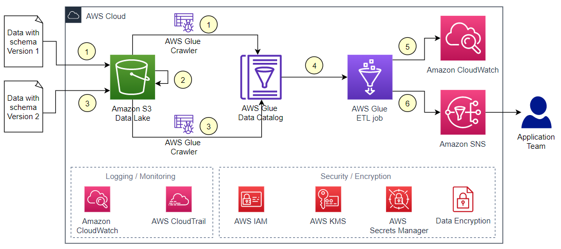
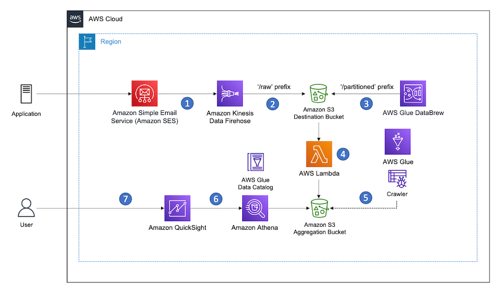
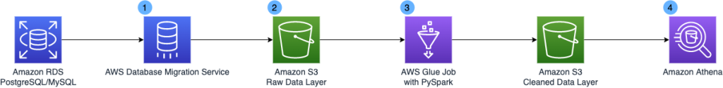
The following diagram illustrates the solution architecture, which contains two major areas:
- Resource deployment (components 1–2) – An AWS Step Functions workflow is run manually on demand to update or deploy the required AWS Glue resources. These AWS Glue resources will be used for landing data into the data lake
- ETL job runs (components 3–6) – The AWS Glue workflows (one per source table) run on the defined schedule, and extract and land data to the data lake raw layer
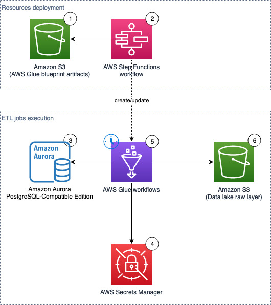
The solution workflow contains the following steps:
- An S3 bucket stores an AWS Glue blueprint (ZIP) and the workflow catalog (JSON file).
- A Step Functions workflow orchestrates the AWS Glue resources creation.
- We use Amazon Aurora as the data source with our sample data, but any PostgreSQL database works with the provided script, or other JDBC sources with customization.
- AWS Secrets Manager stores the secrets of the source databases.
- On the predefined schedule, AWS Glue triggers relevant AWS Glue jobs to perform ETL.
- Extracted data is loaded into an S3 bucket that serves as the data lake raw layer.
Prerequisites
To follow along with this post, complete the following prerequisite steps.
- If you want to use a new database with sample data, you need two private subnets, with a Secrets Manager VPC endpoint associated to the subnets and security groups, and an Amazon S3 VPC endpoint associated to the corresponding route tables.

- If you want to use your existing database either in AWS or on premises as a data source, you need network connectivity (a subnet and security group) for the AWS Glue jobs that can access the source database, Amazon S3, and Secrets Manager.
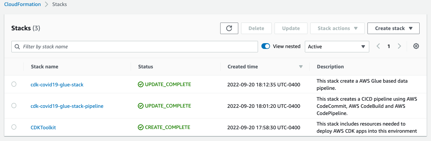
Provision resources with AWS CloudFormation
In this step, we provision our solution resources with AWS CloudFormation.
Database with sample data (optional)
This CloudFormation stack works only in AWS Regions where Amazon Aurora Serverless v1 is supported. Complete the following steps to create a database with sample data:
- Choose Launch Stack.

- On the Create stack page, choose Next.
- For Stack name, enter
demo-database. - For DBSecurityGroup, choose select the security group for the database (for example,
default). - For DBSubnet, choose two or more private subnets to host the database.
- For ETLAZ, choose the Availability Zone for ETL jobs. It must match with
ETLSubnet. - For ETLSubnet, choose the subnet for the jobs. This must match with
ETLAZ.
To find the subnet and corresponding Availability Zone, go to the Amazon Virtual Private Cloud (Amazon VPC) console and look at the columns Subnet ID and Availability Zone.
- Choose Next.
- On the Configure stack options page, skip the inputs and choose Next.
- On the Review page, choose Create stack.
- When the stack is complete, go to the Outputs tab and note the value for
SecretsARN.
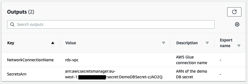
This CloudFormation stack creates the following resources:
- An Amazon Aurora PostgreSQL-Compatible Edition (Serverless v1, engine version 11.13) database
- A Secrets Manager secret (
DemoDBSecret) storing the connection details to the source database - An AWS Glue network connection (
rds_vpc) that can communicate with the source database and Amazon S3
Now you can populate the database with sample data. The data is generated by referencing to the sample HR schema.
- Open the Amazon RDS Query Editor.
- In the Connect to database section, provide the following information:
- For Database instance, enter
demo-<123456789012>. - For Database username, connect with a Secrets Manager ARN.
- For Secrets Manager ARN, enter the ARN from the outputs of the CloudFormation stack.
- For Database name, enter
hr.
- For Database instance, enter
- Choose Connect to database.
- Enter the contents of the SQL file into the editor, then choose Run.
Main stack (required)
This CloudFormation stack works in all AWS Regions.
- Choose Launch Stack.
- On the Create stack page, choose Next.
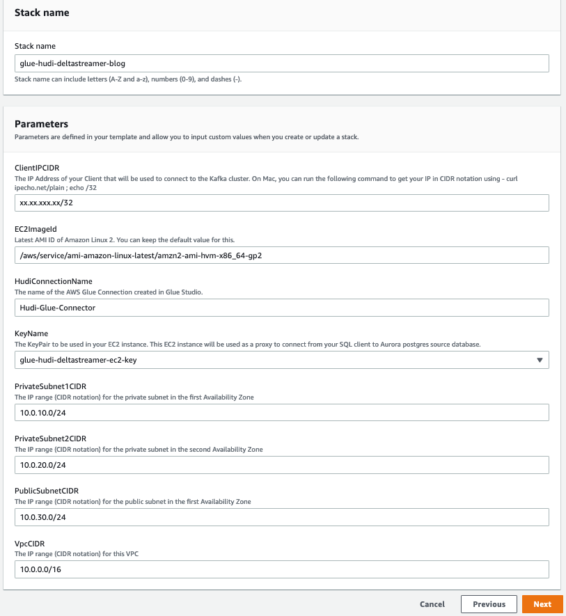
- For Stack name, enter
data-lake-landing. - For BlueprintName, enter a name for your blueprint (default:
data-lake-landing). - For S3BucketNamePrefix, enter a prefix (default:
data-lake-raw-layer). - Choose Next.
- On the Configure stack options page, skip the inputs and choose Next.
- On the Review page, select I acknowledge that AWS CloudFormation might create IAM resources with custom names.
- Choose Create stack.
- When the stack is complete, go to the Outputs tab and note the names of the S3 bucket (for example,
data-lake-raw-layer-123456789012-region) and Step Functions workflow (for example,data-lake-landing).

The CloudFormation stack creates the following resources:
- An S3 bucket as the data lake raw layer
- A Step Functions workflow (see the definition on the GitHub repo)
- AWS Identity and Access Management (IAM) roles and policies for the Step Functions workflow to provision AWS Glue resources and AWS Glue job executions.
The GlueExecutionRole is limited to the DemoDBSecret in Secrets Manager. If you need to connect to other databases which has a different endpoint/address or credentials, don’t forget to create new secrets and grant additional permissions to the IAM role or secrets so your AWS Glue jobs can authenticate with the source databases.
Prepare database connections
If you want to use this solution to perform ETL against your existing databases, follow this section. Otherwise, if you have deployed the CloudFormation stack for the database with sample data, jump to the section “Edit the workflow catalog”.
You need to have a running PostgreSQL database ready. To connect to other database engines, you need to customize this solution, particularly the jdbcUrl in the supplied PySpark script.
Create the database secret
To create your Secrets Manager secret, complete the following steps:
- On the Secrets Manager console, choose Store a new secret.
- For Secret type, choose Credentials for Amazon RDS database or Credentials for other database.
- For Credentials, enter the user name and password to your database.
- For Encryption key, keep the default AWS Key Management Service (AWS KMS) managed key
aws/secretsmanager. - For Database, choose the database instance, or manually input the engine, server address, database name, and port.
- Choose Next.
- For Secret name, enter a name for your secret (for example,
rds-secrets). - Choose Next.
- Skip the Configure rotation – optional page and choose Next.
- Review the summary and choose Store.
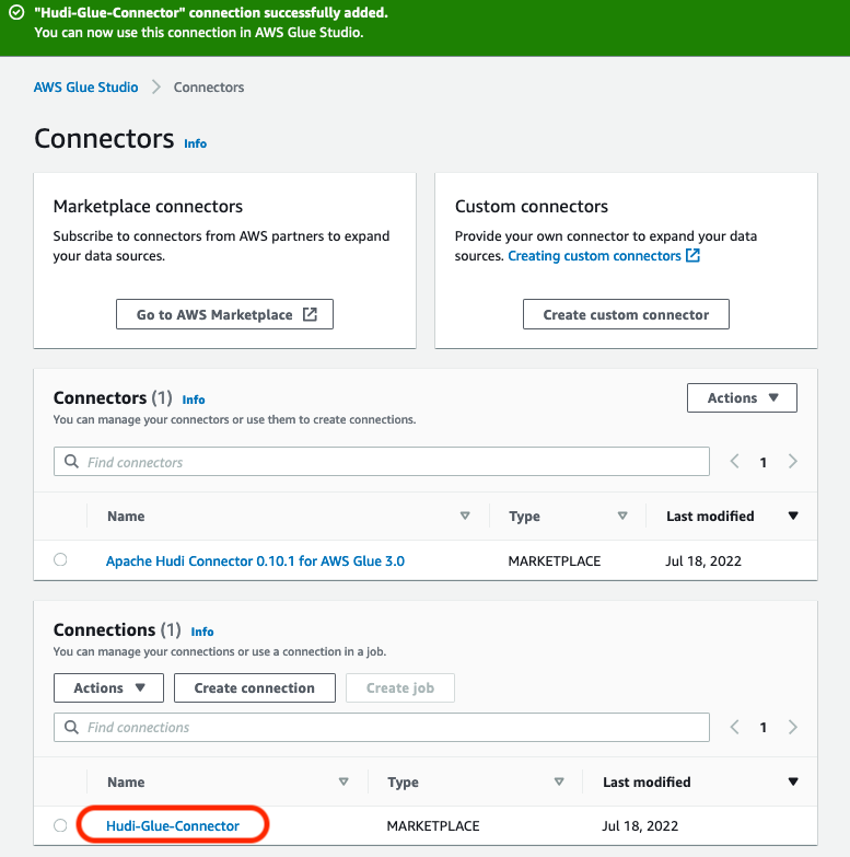
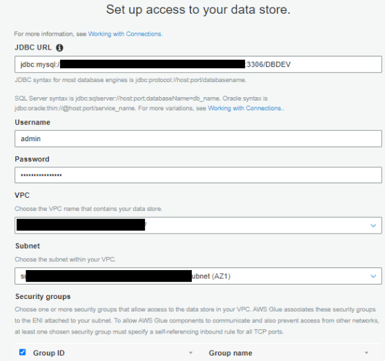
Create the AWS Glue connection
To create your AWS Glue connection, complete the following steps:
- On the AWS Glue Studio console, choose Connectors.
- Under Connections, choose Create connection.
- For Name, enter a name (for example,
rds-vpc). - For Connection type, choose Network.
- For the VPC, subnet, and security groups (prepared in the prerequisite steps), enter where the ETL jobs run and are able to connect to the source database, Amazon S3, and Secrets Manager.
- Choose Create connection.
You’re now ready to configure the rest of the solution.
Edit the workflow catalog
To download the workflow catalog, complete the following steps:
- Download and edit the sample file.
- If you are using the provided sample database, you must change the values of
GlueExecutionRoleandDestinationBucketName. If you are using your own databases, you must change all vaules exceptWorkflowName,JobScheduleType, andScheduleCronPattern.
- Rename the file
your_blueprint_name.jsonand upload it to your S3 bucket (for example,s3://data-lake-raw-layer-123456789012-eu-west-1/data-lake-landing.json).
The example workflow has the JobScheduleType set to Cron. See Time-based schedules for jobs and crawlers for examples setting cron patterns. Alternatively set JobScheduleType to OnDemand.
See blueprint.cfg for the full list of parameters.
The provided workflow catalog JSON file contains job definitions of seven tables: public.regions, public.countries, public.locations, public.departments, public.jobs, public.employees, and public.job_history.
Review the PySpark script (optional)
The sample script performs the following:
- Read the updated records from the source table:
jdbc_df = (spark.read.format("jdbc")
           .option("url", jdbcUrl)
           .option("user", secret["username"])
           .option("password", secret["password"])
           .option("query", sql_query)
           .load()
)- Add the date and timestamp columns:
df_withdate = jdbc_df.withColumn("ingestion_timestamp", lit(current_timestamp()))- Write the DataFrame to Amazon S3 as Parquet files.
Prepare the AWS Glue blueprint
Prepare your AWS Glue blueprint with the following steps:
- Download the sample file and unzip it in your local computer.
- Make any necessary changes to the PySpark script to include your own logic, and compress the three files (
blueprint.cfg,jdbc_to_s3.py,layout.py; exclude any folders) asyour_blueprint_name.zip(for example,data-lake-landing.zip):
- Upload to the S3 bucket (for example,
s3://data-lake-raw-layer-123456789012-region/data-lake-landing.zip).
Now you should have two files uploaded to your S3 bucket.

Run the Step Functions workflow to deploy AWS Glue resources
To run the Step Functions workflow, complete the following steps:
- On the Step Functions console, select your state machine (
data-lake-landing) and choose View details. - Choose Start execution.
- Keep the default values in the pop-up.
- Choose Start execution.
- Wait until the Success step at the bottom turns green.
It’s normal to have some intermediate steps with the status “Caught error.”

When the workflow catalog contains a large number of ETL job entries, you can expect some delays. In our test environment, creating 100 jobs from a clean state can take around 22 minutes; the second run (deleting existing AWS Glue resources and creating 100 jobs) can take around 27 minutes.
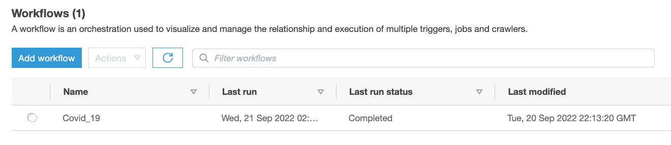
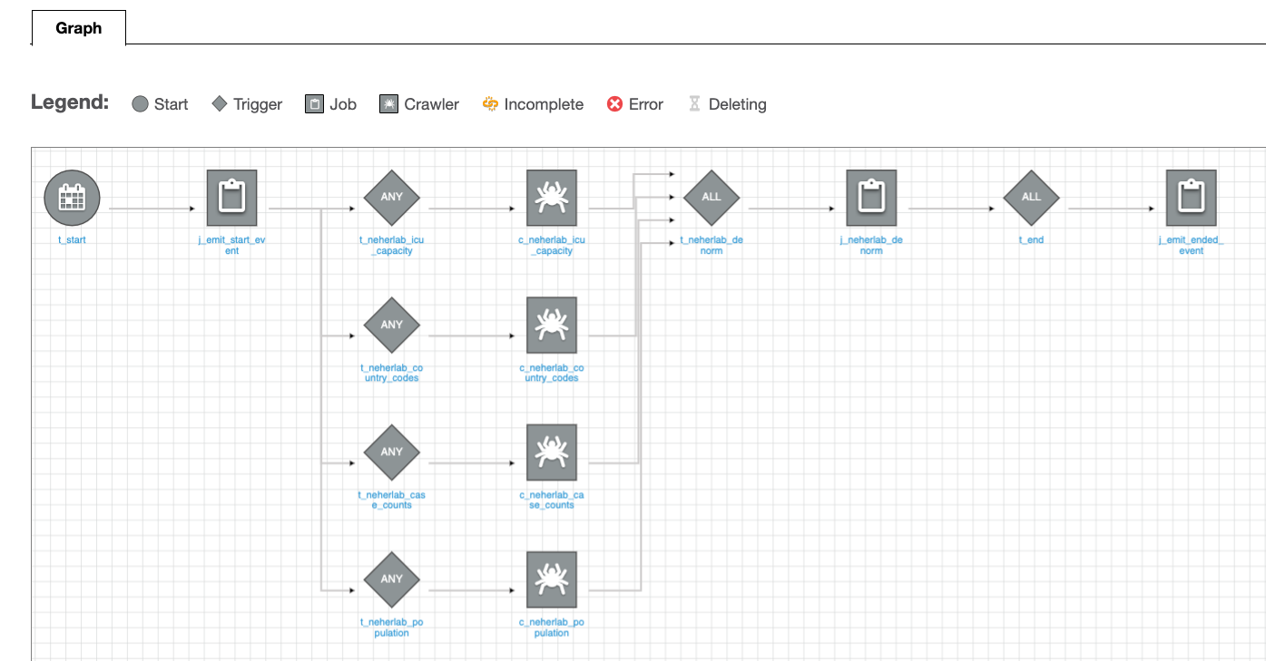
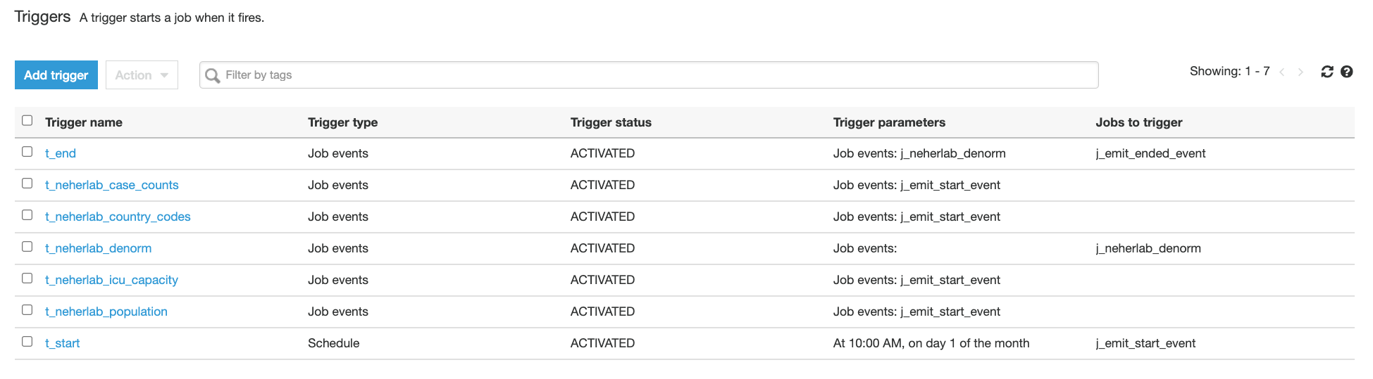
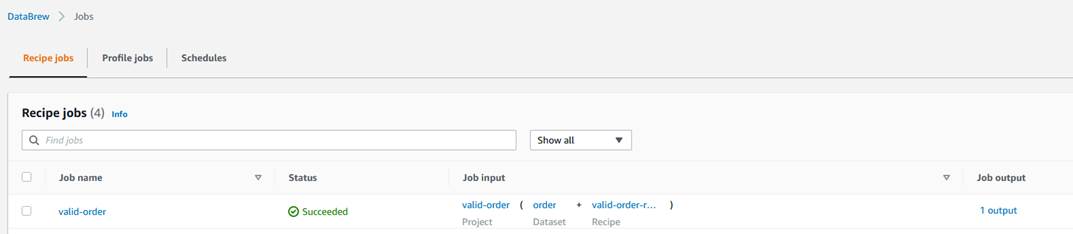
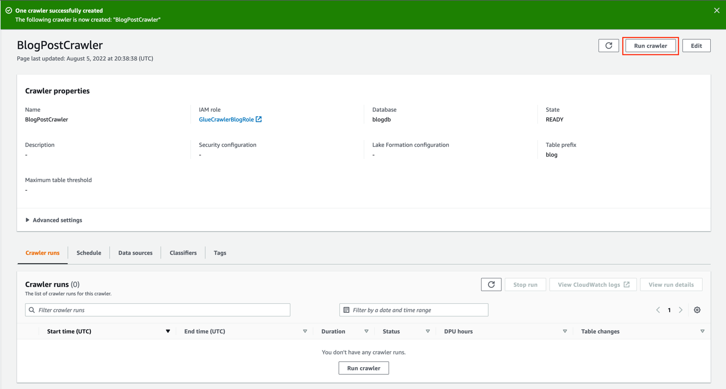
Verify the workflow in AWS Glue
To check the workflow, complete the following steps:
- On the AWS Glue console, choose Workflows.
- Verify that all AWS Glue workflows defined in
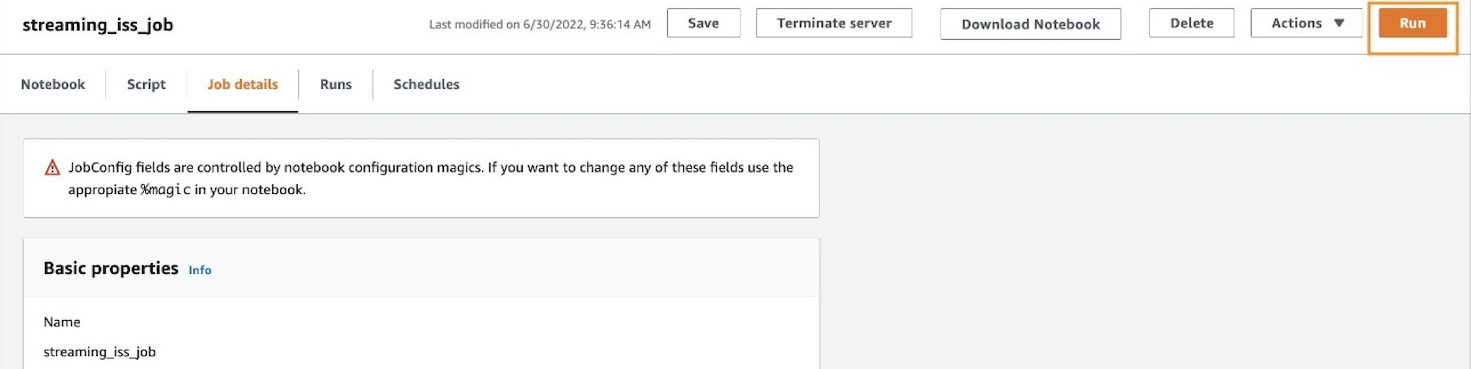
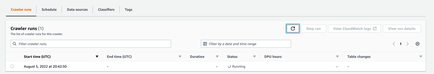
workflow_config.jsonare listed. - Select one of the workflows, and on the Action menu, choose Run.
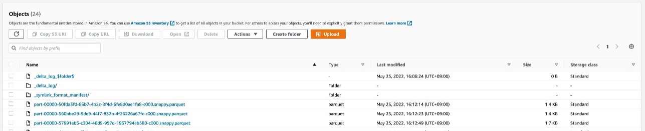
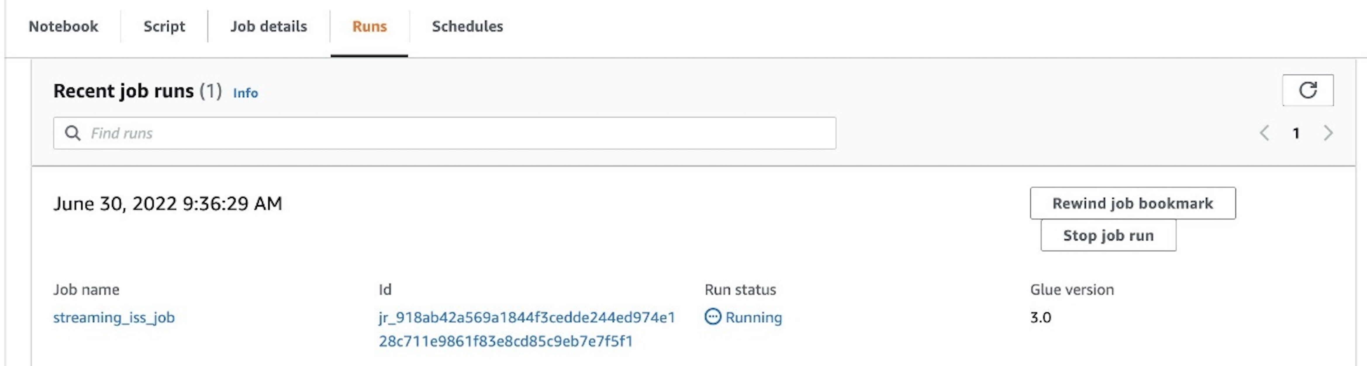
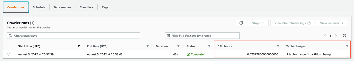
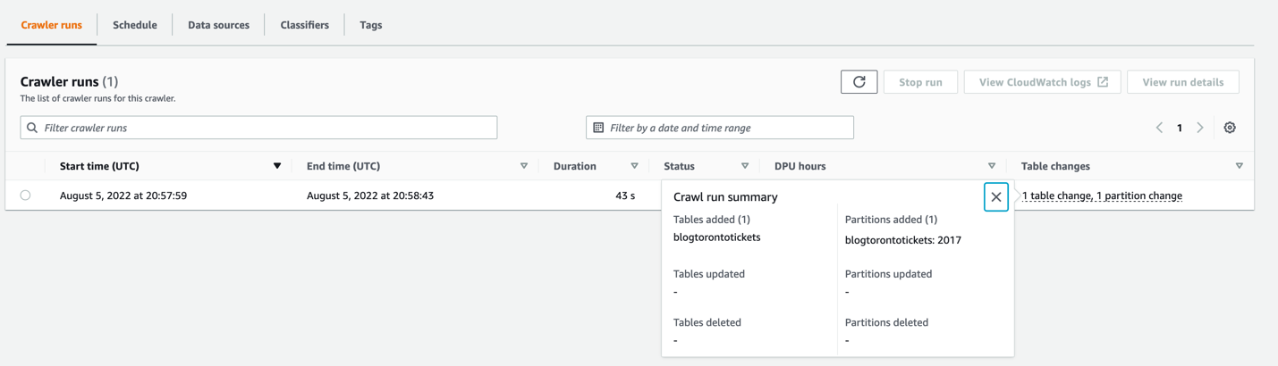
- Wait for about 3 minutes (or longer if not using the provided database with sample data), and verify on the Amazon S3 console that new Parquet files are created in your data lake (for example,
s3://data-lake-raw-layer-123456789012-region/database/table/ingestion_date=yyyy-mm-dd/).

Step Functions workflow overview
This section describes the major steps in the Step Functions workflow.
Register the AWS Glue blueprint
A blueprint allows you to parameterize a workflow (defining jobs and crawlers), and subsequently generate multiple AWS Glue workflows reusing the same code logic to handle similar data ETL activities. The following diagram illustrates the AWS Glue blueprint registration part of the Step Functions workflow.

The step Glue: CreateBlueprint takes the ZIP archive in Amazon S3 (sample) and registers it for later use.
To understand how to develop a blueprint, see Developing blueprints in AWS Glue.
Parse the workflow catalog and clean up resources
The step S3: ParseGlueWorkflowsConfig triggers the following Map state, and runs a set of steps for each element of an input array.

We set the maximum concurrency to five parallel iterations to lower the chance of exceeding the maximum allowed API request rate (per account per Region). For each ETL job definition, the Step Functions workflow cleans up relevant AWS Glue resources (if they exist), including the workflow, job, and trigger.
For more information on the Map state, refer to Map.
Run the AWS Glue blueprint
Within the Map state, the step Glue: CreateWorkflowFromBlueprint starts an asynchronous process to create the AWS Glue workflow (for each job definition), and the jobs and triggers that the workflow encapsulates.

In this solution, all AWS Glue workflows share the same logic, beginning with a trigger to handle the schedule, followed by a job to run the ETL logic.
As indicated by the step CreateWorkflowFailed, any AWS Glue blueprint creation failure stops the whole Step Functions workflow and marks it with a failed status. Note that no rollback will happen. Fix the errors and rerun the Step Functions workflow. This will not result in duplicated AWS Glue resources and existing ones will be cleaned up in the process.
Limitations
Note the following limitations of this solution:
- Each run of the Step Functions workflow deletes all relevant AWS Glue jobs defined in the workflow catalog, and creates new jobs with a different (random) suffix. As a result, you will lose the job run history in AWS Glue. The underlying metrics and logs are retained in Amazon CloudWatch.
Clean up
To avoid incurring future charges, perform the following steps:
- Disable the schedules of the deployed AWS Glue jobs:
- Open the workload configuration file in your S3 bucket (
s3://data-lake-raw-layer-123456789012-eu-west-1/data-lake-landing.json) and replace the value ofJobScheduleTypetoOnDemandfor all workflow definitions. - Run the Step Functions workflow (
data-lake-landing). - Observe that all AWS Glue triggers ending with
_starting_triggerhave the trigger type On-demand instead of Schedule.
- Open the workload configuration file in your S3 bucket (
- Empty the S3 bucket and delete the CloudFormation stack.
- Delete the deployed AWS Glue resources:
- All AWS Glue triggers ending with
_starting_trigger. - All AWS Glue jobs starting with the
WorkflowNamedefined in the workflow catalog. - All AWS Glue workflows with the
WorkflowNamedefined in the workflow catalog. - AWS Glue blueprints.
- All AWS Glue triggers ending with
Conclusion
AWS Glue blueprints allow data engineers to build and maintain AWS Glue jobs landing data from RDBMS to your data lake at scale.By adopting this standardized and reusable approach, instead of maintaining hundreds of AWS Glue jobs, you now keep track the workflow catalog. When you have new tables to land to your data lake, simply add the entries to your workflow catalog and rerun the Step Functions workflow to deploy resources.
We highly encourage you to customize the blueprints for your multi-step data pipeline (for example, detect and mask sensitive data) and make them available to your organization and the AWS Glue community. To get started, see the Performing complex ETL activities using blueprints and workflows in AWS Glue and the sample blueprints on GitHub. If you have any questions, please leave a comment.
About the Authors
 Moustafa Mahmoud is a Solutions Architect of AWS Data Lab with a passion for data integration, data analysis, machine learning, and BI. Moustafa helps customers convert their ideas to a production-ready data product on AWS. He has over 10 years of experience as a data engineer, machine learning practitioner, and software developer. In his spare time, Moustafa loves exploring nature, reading, and spending time with friends and family.
 Corvus Lee is a Solutions Architect of AWS Data Lab. He enjoys all kinds of data-related discussions, and helps customers build MVPs using AWS Databases, Analytics, and Machine Learning services.


 For this specific example, we use the following information for our Azure SQL Instance:


 Jianwei Li is Senior Analytics Specialist TAM. He provides consultant service for AWS enterprise support customers to design and build modern data platform. He has more than 10 years experience in big data and analytics domain. In his spare time, he like running and hiking.
 Narayanan Venkateswaran is an Engineer in the AWS EMR group. He works on developing Hive in EMR. He has over 17 years of work experience in the industry across several companies including Sun Microsystems, Microsoft, Amazon and Oracle. Narayanan also holds a PhD in databases with focus on horizontal scalability in relational stores.
 Partha Sarathi is an Analytics Specialist TAM – at AWS based in Sydney, Australia. He brings 15+ years of technology expertise and helps Enterprise customers optimize Analytics workloads. He has extensively worked on both on-premise and cloud Bigdata workloads along with various ETL platform in his previous roles. He also actively works on conducting proactive operational reviews around the Analytics services like Amazon EMR, Redshift, and OpenSearch.
 Krish is an Enterprise Support Manager responsible for leading a team of specialists in EMEA focused on BigData & Analytics, Databases, Networking and Security. He is also an expert in helping enterprise customers modernize their data platforms and inspire them to implement operational best practices. In his spare time, he enjoys spending time with his family, travelling, and video games.


 Zach Mitchell is a Sr. Big Data Architect. He works within the product team to enhance understanding between product engineers and their customers while guiding customers through their journey to develop data lakes and other data solutions on AWS analytics services.


 Dylan Qu is a Specialist Solutions Architect focused on big data and analytics with Amazon Web Services. He helps customers architect and build highly scalable, performant, and secure cloud-based solutions on AWS.