Tag Archives: AWS re:Invent

New – AWS Systems Manager Fleet Manager

Post Syndicated from Steve Roberts original https://aws.amazon.com/blogs/aws/new-aws-systems-manager-fleet-manager/

Organizations, and their systems administrators, routinely face challenges in managing increasingly diverse portfolios of IT infrastructure across cloud and on-premises environments. Different tools, consoles, services, operating systems, procedures, and vendors all contribute to complicate relatively common, and related, management tasks. As workloads are modernized to adopt Linux and open-source software, those same systems administrators, who may be more familiar with GUI-based management tools from a Windows background, have to continually adapt and quickly learn new tools, approaches, and skill sets.

AWS Systems Manager is an operational hub enabling you to manage resources on AWS and on-premises. Available today, Fleet Manager is a new console based experience in Systems Manager that enables systems administrators to view and administer their fleets of managed instances from a single location, in an operating-system-agnostic manner, without needing to resort to remote connections with SSH or RDP. As described in the documentation, managed instances includes those running Windows, Linux, and macOS operating systems, in both the AWS Cloud and on-premises. Fleet Manager gives you an aggregated view of your compute instances regardless of where they exist.

All that’s needed, whether for cloud or on-premises servers, is the Systems Manager agent installed on each server to be managed, some AWS Identity and Access Management (IAM) permissions, and AWS Key Management Service (KMS) enabled for Systems Manager‘s Session Manager. This makes it an easy and cost-effective approach for remote management of servers running in multiple environments without needing to pay the licensing cost of expensive management tools you may be using today. As noted earlier, it also works with instances running macOS. With the agent software and permissions set up, Fleet Manager enables you to explore and manage your servers from a single console environment. For example, you can navigate file systems, work with the registry on Windows servers, manage users, and troubleshoot logs (including viewing Windows event logs) and monitor common performance counters without needing the Amazon CloudWatch agent to be installed.

Exploring an Instance With Fleet Manager
To get started exploring my instances using Fleet Manager, I first head to the Systems Manager console. There, I select the new Fleet Manager entry on the navigation toolbar. I can also select the Managed Instances option – Fleet Manager replaces Managed Instances going forward, but the original navigation toolbar entry will be kept for backwards compatibility for a short while. But, before we go on to explore my instances, I need to take you on a brief detour.

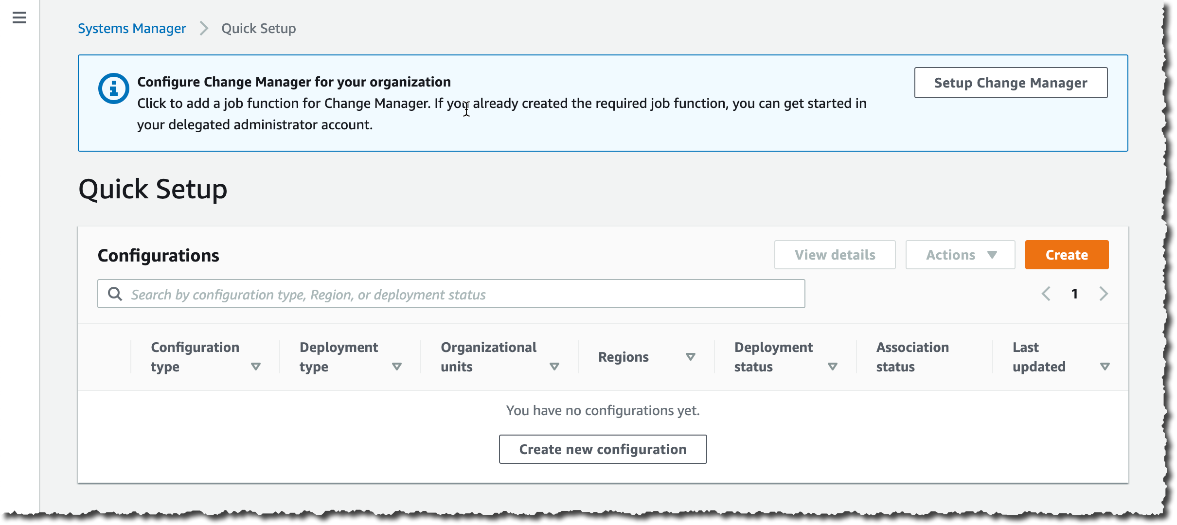
When you select Fleet Manager, as with some other views in Systems Manager, a check is performed to verify that a role, named AmazonSSMRoleForInstancesQuickSetup, exists in your account. If you’ve used other components of Systems Manager in the past, it’s quite possible that it does. The role is used to permit Systems Manager to access your instances on your behalf and if the role exists, then you’re directed to the requested view. If however the role doesn’t exist, you’ll first be taken to the Quick Setup view. This in itself will trigger creation of the role, but you might want to explore the capabilities of Quick Setup, which you can also access any time from the navigation toolbar.

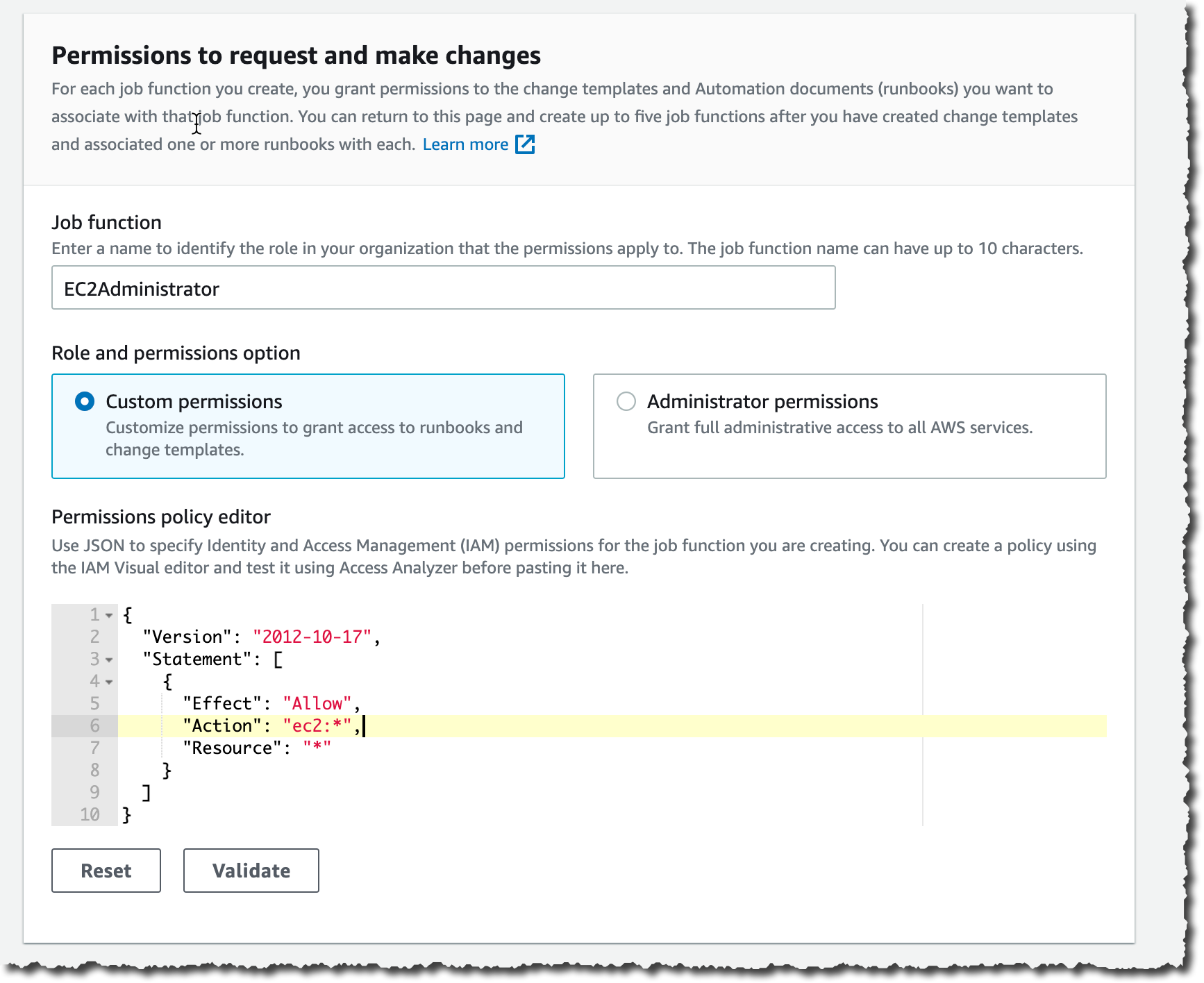
Quick Setup is a feature of Systems Manager that you can use to set up specific configuration items, such as the Systems Manager and CloudWatch agents on your instances (and keep them up-to-date), and also IAM roles permitting access to your resources for Systems Manager components. For this post, all the instances I’m going to use already have the required agent set up, including the role permissions, so I’m not going to discuss this view further but I encourage you to check it out. I also want to remind you that to take full advantage of Fleet Manager‘s capabilities you first need to have KMS encryption enabled for your instances and secondly, the role attached to your Amazon Elastic Compute Cloud (EC2) instances must have the kms:Decrypt role permission included, referencing the key you selected when you enabled KMS encryption. You can enable encryption, and select the KMS key, using the Preferences section of the Session Manager console, and of course you can set up the role permission in the IAM console.

That’s it for the diversion; if you have the role already, as I do, you’ll now be at the Managed instances list view. If you’re at Quick Setup instead, simply click the Fleet Manager navigation button once more.

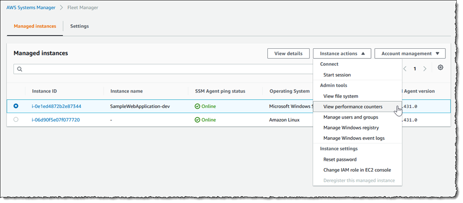
The Managed instances view shows me all of my instances, in the cloud or on-premises, that I can access. Selecting an instance, in this case an EC2 Windows instance launched using AWS Elastic Beanstalk, and clicking Instance actions presents me with a menu of options. The options (less those specific to Windows) are available for my Amazon Linux instance too, and for instances running macOS I can use the View file system option.

Screenshot of <span title="">Fleet Manager</span>'s Managed instances view

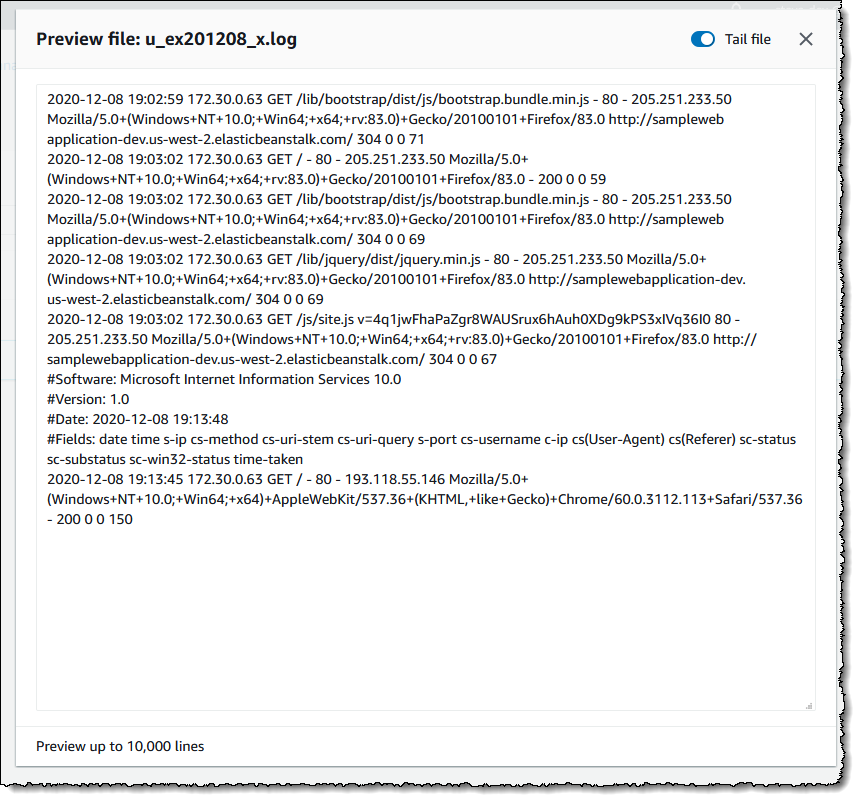
The File system view displays a read-only view onto the file system of the selected instance. This can be particularly useful for viewing text-based log files, for example, where I can preview up to 10,000 lines of a log file and even tail it to view changes as the log updates. I used this to open and tail an IIS web server log on my Windows Server instance. Having selected the instance, I next select View file system from the Instance actions dropdown (or I can click the Instance ID to open a view onto that instance and select File system from the menu displayed on the instance view).

Having opened the file system view for my instance, I navigate to the folder on the instance containing the IIS web server logs.

Screenshot of <span title="">Fleet Manager</span>'s File system view

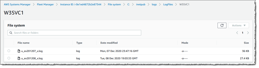
Selecting a log file, I then click Actions and select Tail file. This opens a view onto the log file contents, which updates automatically as new content is written.

Screenshot of tailing a log file in <span title="">Fleet Manager</span>

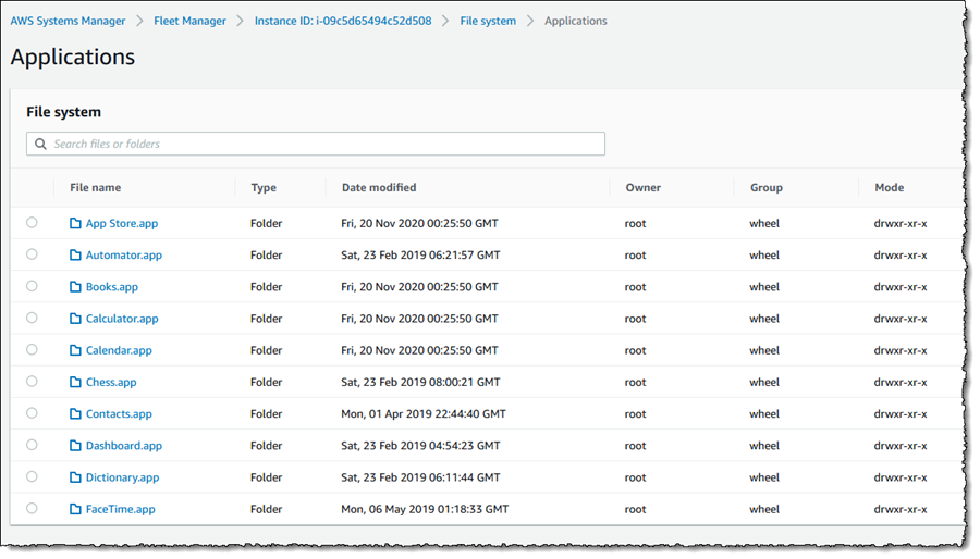
As I mentioned, the File system view is also accessible for macOS-based instances. For example, here is a screenshot of viewing the Applications folder on an EC2 macOS instance.

Screenshot of macOS file system view in <span title="">Fleet Manager</span>

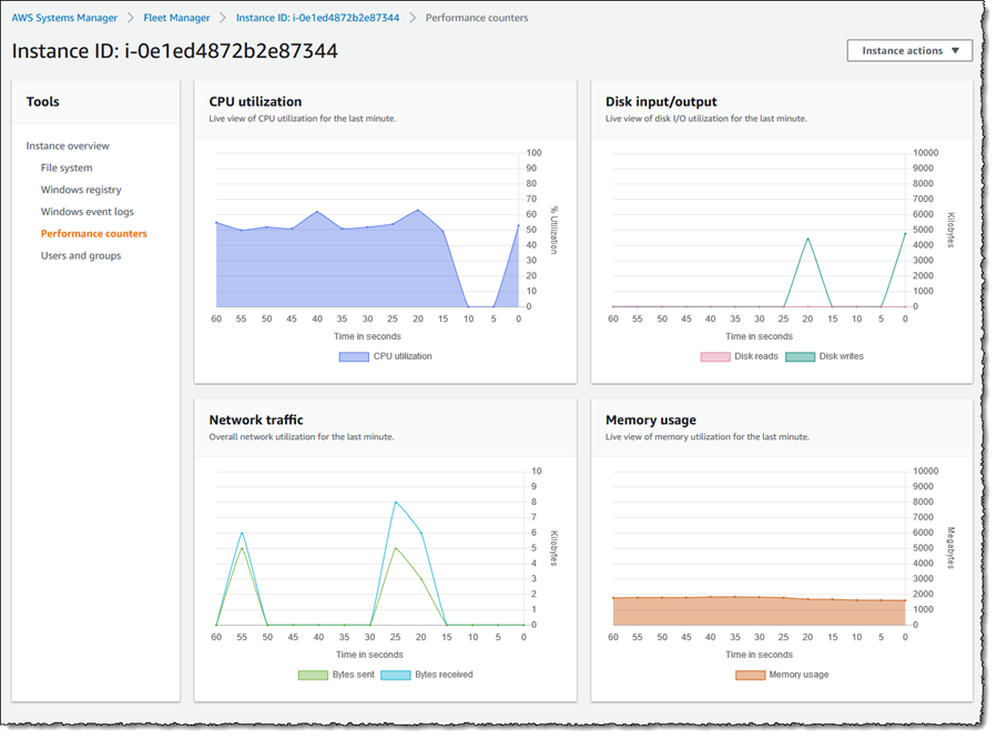
Next, let’s examine the Performance counters view, which is available for both Windows and Linux instances. This view displays CPU, memory, network traffic, and disk I/O and will be familiar to Windows users from Task Manager. The metrics shown reflect the guest OS metrics, whereas EC2 instance metrics you may be used to relate to the hypervisor. On this particular instance I’ve deployed an ASP.NET Core 5 application, which generates a varying length collection of Fibonacci numbers on page refresh. Below is a snapshot of the counters, after I’ve put the instance under a small amount of load. The view updates automatically every 5 seconds.

Screenshot of <span title="">Fleet Manager</span>'s Performance Counters view

There are more views available than I have space for in this post. Using the Windows Registry view, I can view and edit the registry on the selected Windows instance. Windows event logs gives me access to the Application and Service logs, and common Windows logs such as System, Setup, Security, etc. With Users and groups I can manage users or groups, including assignment of users to groups (again for both Windows and Linux instances). For all views, Fleet Manager enables me to use a single and convenient console.

Getting Started
AWS Systems Manager Fleet Manager is available today for use with managed instances running Windows, Linux, and macOS. Information on pricing, for this and other Systems Manager features, can be found at this page.

Learn more, and get started with Fleet Manager today, at AWS Systems Manager.

— Steve

Introducing AWS Systems Manager Change Manager

Post Syndicated from Sébastien Stormacq original https://aws.amazon.com/blogs/aws/introducing-systems-manager-change-manager/

Because you are constantly listening to the feedback from your customer, you are iterating, innovating, and improving your applications and infrastructures. You continually modify your IT systems in the cloud. And let’s face it, changing something in a working system risks breaking things or introducing side effects that are sometimes unpredictable; it doesn’t matter how many tests you do. On the other hand, not making changes is stasis, followed by irrelevance, followed by death.

This is why organizations of all sizes and types have embraced a culture of controlling changes. Some organizations adopt change management processes such as the ones defined in ITIL v4. Some have adopted DevOps’ Continuous Deployment, or other methods. In any case, to support your change management processes, it is important to have tools.

Today, we are launching AWS Systems Manager Change Manager, a new change management capability for AWS Systems Manager. It simplifies the way ops engineers track, approve, and implement operational changes to their application configurations and infrastructures.

Using Change Manager has two primary advantages. First, it can improve the safety of changes made to application configurations and infrastructures, reducing the risk of service disruptions. It makes operational changes safer by tracking that only approved changes are being implemented. Secondly, it is tightly integrated with other AWS services, such as AWS Organizations and AWS Single Sign-On, or the integration with the Systems Manager change calendar and Amazon CloudWatch alarms.

Change Manager provides accountability with a consistent way to report and audit changes made across your organization, their intent, and who approved and implemented them.

Change Manager works across AWS Regions and multiple AWS accounts. It works closely with Organizations and AWS SSO to manage changes from a central point and to deploy them in a controlled way across your global infrastructure.

Terminology
You can use AWS Systems Manager Change Manager on a single AWS account, but most of the time, you will use it in a multi-account configuration.

The way you manage changes across multiple AWS accounts depends on how these accounts are linked together. Change Manager uses the relationships between your accounts defined in AWS Organizations. When using Change Manager, there are three types of accounts:

  • The management account – also known as the “main account” or “root account.” The management account is the root account in an AWS Organizations hierarchy. It is the management account by virtue of this fact.
  • The delegated administrator account – A delegated administrator account is an account that has been granted permission to manage other accounts in Organizations. In the Change Manager context, this is the account from which change requests will be initiated. You will typically log in to this account to manage templates and change requests. Using a delegated administrators account allows you to limit connections made to the root account. It also allows you to enforce a least privileges policy by using a specific subset of permissions required by the changes.
  • The member accounts – Member accounts are accounts that are not the management account or a delegated administrator account, but are still included in Organizations. In my mental model for Change Manager, these would be the accounts that hold the resources where changes are deployed. A delegated administrator account would initiate a change request that would impact resources in a member account. System administrators are discouraged from logging directly into these accounts.

Let’s see how you can use AWS Systems Manager Change Manager by taking a short walk-through demo.

One-Time Configuration
In this scenario, I show you how to use Change Manager with multiple AWS accounts linked together with Organizations. If you are not interested in the one-time configuration, jump to the Create a Change Request section below.

There are four one-time configuration actions to take before using Change Manager: one action in the root account and three in the delegated administrator account. In the root account, I use Quick Setup to define my delegated administrator account and initially configure permissions on the accounts. In the delegated administrator account, you define your source of user identities, you define what users have permissions to approve change templates, and you define a change request template.

First, I ensure I have an Organization in place and my AWS accounts are organized in Organizational Units (OU). For the purpose of this simple example, I have three accounts: the root account, the delegated administrator account in the management OU and a member account in the managed OU. When ready, I use Quick Setup on the root account to configure my accounts. There are multiple paths leading to Quick Setup; for this demo, I use the blue banner on top of the Quick Setup console, and I click Setup Change Manager.

Change Manager Quick Setup


On the Quick Setup page, I enter the ID of the delegated administrator account if I haven’t defined it already. Then I choose the permissions boundaries I grant to the delegated administrator account to perform changes on my behalf. This is the maximum permissions Change Manager receives to make changes. I will further restrict this permission set when I create change requests in a few minutes. In this example, I grant Change Manager permissions to call any ec2 API. This effectively authorizes Change Manager to only run changes related to EC2 instances.

Change Manager Quick Setup

Lower on the screen, I choose the set of accounts that are targets for my changes. I choose between Entire organization or Custom to select one or multiple OUs.

Change Manager Quick Setup 2

After a while, Quick Setup finishes configuring my AWS accounts permission and I can move to the second part of the one-time setup.

Change Manager Quick Setup 3

Second, I switch to my delegated administrator account. Change Manager asks me how I manage users in my organization: with AWS Identity and Access Management (IAM) or AWS Single Sign-On? This defines where Change Manager pulls user identities when I choose approvers. This is a one-time configuration option. This can be changed at any time in the Change Manager Settings page.

Change Manager Settings

Third, on the same page, I define an Amazon Simple Notification Service (SNS) topic to receive notifications about template reviews. This channel is notified any time a template is created or modified, to let template approvers review and approve templates. I also define the IAM (or SSO) user with permission to approve change templates (more about these in one minute).

Change Manager Template Reviewers

Optionally, you can use the existing AWS Systems Manager Change Calendar to define the periods where changes are not authorized, such as marketing events or holiday sales.

Finally, I define a change template. Every change request is created from a template. Templates define common parameters for all change requests based on them, such as the change request approvers, the actions to perform, or the SNS topic to send notifications of progress. You can enforce the review and approval of templates before they can be used. It makes sense to create multiple templates to handle different type of changes. For example, you can create one template for standard changes, and one for emergency changes that overrides the change calendar. Or you can create different templates for different types of automation run books (documents).

To help you to get started, we created a template for you: the “Hello World” template. You can use it as a starting point to create a change request and test out your approval flow.

At any time, I can create my own template. Let’s imagine my system administrator team is frequently restarting EC2 instances. I create a template allowing them to create change requests to restart one or multiple instances. Using the delegated administrator account, I navigate to the Change Manager management console and click Create template.

Change Manager Create Template

In a nutshell, a template defines the list of authorized actions, where to send notifications and who can approve the change request. Actions are an AWS Systems Manager runbook. Emergency change templates allow change requests to bypass the change calendar I wrote about earlier. Under Runbook Options, I choose one or multiple runbooks allowed to run. For this example, I choose the AWS EC2RestartInstance runbook.

I use the console to create the template, but templates are defined internally as YAML. I can edit the YAML using the Editor tab, or when I am using the AWS Command Line Interface (CLI) or API. This means I can version control them just like the rest of my infrastructure (as code).Change Manager Create Template part 1

Just below, I document my template using text formatted as markdown format. I use this section to document the defining characteristics of the template and provide any necessary instructions, such as back-out procedures, to the requestor.

Change Manager Template Documentation

I scroll down that page and click Add Approver to define approvers. Approvers can be individual users or groups. The list of approvers are defined either at the template level or in the change request itself. I also choose to create an SNS topic to inform approvers when any requests are created that require their approval.

In the Monitoring section I select the alarm that, when active, stops any change based on this template, and initiate a rollback.

In the Notifications section, I select or create another SNS topic so I’m notified when status changes for this template occur.

Change Manager Create Template part 2

Once I am done, I save the template and submit it for review.

Change Manager Submit Template for Review

Templates have to be reviewed and approved before they can be used. To approve the template, I connect the console as the template_approver user I defined earlier. As template_approver user, I see pending approvals on the Overview tab. Or, I navigate to the Templates tab, select the template I want to review. When I am done reviewing it, I click Approve.

Change Manager Approve Template

Voila, now we’re ready to create change requests based on this template. Remember that all the preceding steps are one-time configurations and can be amended at any time. When existing templates are modified, the changes go through a review and approval process again.

Create a Change Request
To create a change request on any account linked to the Organization, I open a AWS Systems Manager Change Manager console from the delegated administrator account and click Create request.

Change Manager Create Request

I choose the template I want to use and click Next.

Change Manager Select Template I enter a name for this change request. The change is initiated immediately after all approvals are granted, or I specify an optional scheduled time. When the template allows me, I choose the approver for this change. In this example, the approver is defined by the template and cannot be changed. I click Next.

Change Manager Create CR part 1

On the next screen, there are multiple important configuration options, relating to the actual execution of the change:

  • Target location – lets me define on which target AWS accounts and AWS Region I want to run this change.
  • Deployment target – lets me define which resources are the target of this change. One EC2 instance? Or multiple ones identified by their tags, their resources groups, a list of instance IDs, or all EC2 instances.
  • Runbook parameters – lets me define the parameters I want to pass to my runbook, if any.
  • Execution role – lets me define the set of permissions I grant the System Manager to deploy with this change. The permission set must have service changemanagement.ssm.amazonaws.com as principal for the trust policy. Selecting a role allows me to grant the Change Manager runtime a different permission set than the one I have.

Here is an example allowing Change Manager to stop an EC2 instance (you can scope it down to a specific AWS account, specific Region, or specific instances):

{
    "Version": "2012-10-17",
    "Statement": [
        {
            "Effect": "Allow",
            "Action": [
                "ec2:StartInstances",
                "ec2:StopInstances"
            ],
            "Resource": "*",
        },
        {
            "Effect": "Allow",
            "Action": "ec2:DescribeInstances",
            "Resource": "*"
        }
    ]
}

And the associated trust policy:

{
  "Version": "2012-10-17",
  "Statement": [
    {
      "Effect": "Allow",
      "Principal": {
        "Service": "changemanagement.ssm.aws.internal"
      },
      "Action": "sts:AssumeRole"
    }
  ]
}

When I am ready, I click Next. On the last page, I review my data entry and click Submit for approval.

At this stage, the approver receives a notification, based on the SNS topic configured in the template. To continue this demo, I sign out of the console and sign in again as the cr_approver user, which I created, with permission to view and approve change requests.

As the cr_approver user, I navigate to the console, review the change request, and click Approve.

Change Manager Review Change Request

The change request status switches to scheduled, and eventually turns green to Success. At any time, I can click the change request to get the status, and to collect errors, if any.

Change Manager Dashboard with Succeeded Request

I click on the change request to see the details. In particular, the Timeline tab shows the history of this CR.

Change Management CR Timeline

Availability and Pricing
AWS Systems Manager Change Manager is available today in all commercial AWS Regions, except mainland China. The pricing is based on two dimensions: the number of change requests you submit and the total number of API calls made. The number of change requests you submit will be the main cost factor. We will charge $0.29 per change request. Check the pricing page for more details.

You can evaluate Change Manager for free for 30 days, starting on your first change request.

As usual, let us know what you think and let’s get started today

— seb

AWS CloudShell – Command-Line Access to AWS Resources

Post Syndicated from Jeff Barr original https://aws.amazon.com/blogs/aws/aws-cloudshell-command-line-access-to-aws-resources/

No matter how much automation you have built, no matter how great you are at practicing Infrastructure as Code (IAC), and no matter how successfully you have transitioned from pets to cattle, you sometimes need to interact with your AWS resources at the command line. You might need to check or adjust a configuration file, make a quick fix to a production environment, or even experiment with some new AWS services or features.

Some of our customers feel most at home when working from within a web browser and have yet to set up or customize their own command-line interface (CLI). They tell is that they don’t want to deal with client applications, public keys, AWS credentials, tooling, and so forth. While none of these steps are difficult or overly time-consuming, they do add complexity and friction and we always like to help you to avoid both.

Introducing AWS CloudShell
Today we are launching AWS CloudShell, with the goal of making the process of getting to an AWS-enabled shell prompt simple and secure, with as little friction as possible. Every shell environment that you run with CloudShell has the AWS Command Line Interface (CLI) (v2) installed and configured so you can run aws commands fresh out of the box. The environments also include the Python and Node runtimes, with many more to come in the future.

To get started, I simply click the CloudShell icon in the AWS Management Console:

My shell sets itself up in a matter of seconds and I can issue my first aws command immediately:

The shell environment is based on Amazon Linux 2. I can store up to 1 GB of files per region in my home directory and they’ll be available each time I open a shell in the region. This includes shell configuration files such as .bashrc and shell history files.

I can access the shell via SSO or as any IAM principal that can login to the AWS Management Console, including federated roles. In order to access CloudShell, the AWSCloudShellFullAccess policy must be in effect. The shell runs as a normal (non-privileged) user, but I can sudo and install packages if necessary.

Here are a couple of features that you should know about:

Themes & Font Sizes – You can switch between light and dark color themes, and choose any one of five font sizes:

Tabs and Sessions – You can have multiple sessions open within the same region, and you can control the tabbing behavior, with options to split horizontally and vertically:

You can also download files from the shell environment to your desktop, and upload them from your desktop to the shell.

Things to Know
Here are a couple of important things to keep in mind when you are evaluating CloudShell:

Timeouts & Persistence – Each CloudShell session will timeout after 20 minutes or so of inactivity, and can be reestablished by refreshing the window:

RegionsCloudShell is available today in the US East (N. Virginia), US East (Ohio), US West (Oregon), Europe (Ireland), and Asia Pacific (Tokyo) Regions, with the remaining regions on the near-term roadmap.

Persistent Storage – Files stored within $HOME persist between invocations of CloudShell with a limit of 1 GB per region; all other storage is ephemeral. This means that any software that is installed outside of $HOME will not persist, and that no matter what you change (or break), you can always begin anew with a fresh CloudShell environment.

Network Access – Sessions can make outbound connections to the Internet, but do not allow any type of inbound connections. Sessions cannot currently connect to resources inside of private VPC subnets, but that’s also on the near-term roadmap.

Runtimes – In addition to the Python and Node runtimes, Bash, PowerShell, jq, git, the ECS CLI, the SAM CLI, npm, and pip already installed and ready to use.

Pricing – You can use up to 10 concurrent shells in each region at no charge. You only pay for other AWS resources you use with CloudShell to create and run your applications.

Try it Out
AWS CloudShell is available now and you can start using it today. Launch one and give it a try, and let us know what you think!

Jeff;

re:Invent 2020 Liveblog: Werner Vogels Keynote

Post Syndicated from AWS News Blog Team original https://aws.amazon.com/blogs/aws/reinvent-2020-liveblog-werner-vogels-keynote/

Join us Tuesday, Dec. 15 for Dr. Werner Vogels’ Keynote as he shares how Amazon is solving today’s hardest technology problems. Jeff Barr, Martin Beeby, Steve Roberts and Channy Yun will liveblog the event, sharing all the highlights, insights and major announcements from this final keynote of re:Invent 2020.

See you here Tuesday, 7:30-10:00 AM (PST)!


New – VPC Reachability Analyzer

Post Syndicated from Harunobu Kameda original https://aws.amazon.com/blogs/aws/new-vpc-insights-analyzes-reachability-and-visibility-in-vpcs/

With Amazon Virtual Private Cloud (VPC), you can launch a logically isolated customer-specific virtual network on the AWS Cloud. As customers expand their footprint on the cloud and deploy increasingly complex network architectures, it can take longer to resolve network connectivity issues caused by misconfiguration. Today, we are happy to announce VPC Reachability Analyzer, a network diagnostics tool that troubleshoots reachability between two endpoints in a VPC, or within multiple VPCs.

Ensuring Your Network Configuration is as Intended
You have full control over your virtual network environment, including choosing your own IP address range, creating subnets, and configuring route tables and network gateways. You can also easily customize the network configuration of your VPC. For example, you can create a public subnet for a web server that has access to the Internet with Internet Gateway. Security-sensitive backend systems such as databases and application servers can be placed on private subnets that do not have internet access. You can use multiple layers of security, such as security groups and network access control list (ACL), to control access to entities of each subnet by protocol, IP address, and port number.

You can also combine multiple VPCs via VPC peering or AWS Transit Gateway for region-wide, or global network connections that can route traffic privately. You can also use VPN Gateway to connect your site with your AWS account for secure communication. Many AWS services that reside outside the VPC, such as AWS Lambda, or Amazon S3, support VPC endpoints or AWS PrivateLink as entities inside the VPC and can communicate with those privately.

When you have such rich controls and feature set, it is not unusual to have unintended configuration that could lead to connectivity issues. Today, you can use VPC Reachability Analyzer for analyzing reachability between two endpoints without sending any packets. VPC Reachability analyzer looks at the configuration of all the resources in your VPCs and uses automated reasoning to determine what network flows are feasible. It analyzes all possible paths through your network without having to send any traffic on the wire. To learn more about how these algorithms work checkout this re:Invent talk or read this paper.

How VPC Reachability Analyzer Works
Let’s see how it works. Using VPC Reachability Analyzer is very easy, and you can test it with your current VPC. If you need an isolated VPC for test purposes, you can run the AWS CloudFormation YAML template at the bottom of this article. The template creates a VPC with 1 subnet, 2 security groups and 3 instances as A, B, and C. Instance A and B can communicate with each other, but those instances cannot communicate with instance C because the security group attached to instance C does not allow any incoming traffic.

You see Reachability Analyzer in the left navigation of the VPC Management Console.

Click Reachability Analyzer, and also click Create and analyze path button, then you see new windows where you can specify a path between a source and destination, and start analysis.

You can specify any of the following endpoint types: VPN Gateways, Instances, Network Interfaces, Internet Gateways, VPC Endpoints, VPC Peering Connections, and Transit Gateways for your source and destination of communication. For example, we set instance A for source and the instance B for destination. You can choose to check for connectivity via either the TCP or UDP protocols. Optionally, you can also specify a port number, or source, or destination IP address.

Configuring test path

Finally, click the Create and analyze path button to start the analysis. The analysis can take up to several minutes depending on the size and complexity of your VPCs, but it typically takes a few seconds.

You can now see the analysis result as Reachable. If you click the URL link of analysis id nip-xxxxxxxxxxxxxxxxx, you can see the route hop by hop.

The communication from instance A to instance C is not reachable because the security group attached to instance C does not allow any incoming traffic.

If you click nip-xxxxxxxxxxxxxxxxx for more detail, you can check the Explanations for details.

Result Detail

Here we see the security group that blocked communication. When you click on the security group listed in the upper right corner, you can go directly to the security group editing window to change the security group rules. In this case adding a properly scoped ingress rule will allow the instances to communicate.

Available Today
This feature is available for all AWS commercial Regions except for China (Beijing), and China (Ningxia) regions. More information is available in our technical documentation, and remember that to use this feature your IAM permissions need to be set up as documented here.

– Kame

CloudFormation YAML template for test

---
Description: An AWS VPC configuration with 1 subnet, 2 security groups and 3 instances. When testing ReachabilityAnalyzer, this provides both a path found and path not found scenario.
AWSTemplateFormatVersion: 2010-09-09

Mappings:
  RegionMap:
    us-east-1:
      execution: ami-0915e09cc7ceee3ab
      ecs: ami-08087103f9850bddd

Resources:
  # VPC
  VPC:
    Type: AWS::EC2::VPC
    Properties:
      CidrBlock: 172.0.0.0/16
      EnableDnsSupport: true
      EnableDnsHostnames: true
      InstanceTenancy: default

  # Subnets
  Subnet1:
    Type: AWS::EC2::Subnet
    Properties:
      VpcId: !Ref VPC
      CidrBlock: 172.0.0.0/20
      MapPublicIpOnLaunch: false

  # SGs
  SecurityGroup1:
    Type: AWS::EC2::SecurityGroup
    Properties:
      GroupDescription: Allow all ingress and egress traffic
      VpcId: !Ref VPC
      SecurityGroupIngress:
        - CidrIp: 0.0.0.0/0
          IpProtocol: "-1" # -1 specifies all protocols

  SecurityGroup2:
    Type: AWS::EC2::SecurityGroup
    Properties:
      GroupDescription: Allow all egress traffic
      VpcId: !Ref VPC

  # Instances
  # Instance A and B should have a path between them since they are both in SecurityGroup 1
  InstanceA:
    Type: AWS::EC2::Instance
    Properties:
      ImageId:
        Fn::FindInMap:
          - RegionMap
          - Ref: AWS::Region
          - execution
      InstanceType: 't3.nano'
      SubnetId:
        Ref: Subnet1
      SecurityGroupIds:
        - Ref: SecurityGroup1

  # Instance A and B should have a path between them since they are both in SecurityGroup 1
  InstanceB:
    Type: AWS::EC2::Instance
    Properties:
      ImageId:
        Fn::FindInMap:
          - RegionMap
          - Ref: AWS::Region
          - execution
      InstanceType: 't3.nano'
      SubnetId:
        Ref: Subnet1
      SecurityGroupIds:
        - Ref: SecurityGroup1

  # This instance should not be reachable from Instance A or B since it is in SecurityGroup 2
  InstanceC:
    Type: AWS::EC2::Instance
    Properties:
      ImageId:
        Fn::FindInMap:
          - RegionMap
          - Ref: AWS::Region
          - execution
      InstanceType: 't3.nano'
      SubnetId:
        Ref: Subnet1
      SecurityGroupIds:
        - Ref: SecurityGroup2


re:Invent 2020 Liveblog: Infrastructure Keynote

Post Syndicated from AWS News Blog Team original https://aws.amazon.com/blogs/aws/reinvent-2020-liveblog-infrastructure-keynote/

Join us Thursday, Dec. 10 from 7:30-9:30 AM (PST) as we liveblog the AWS re:Invent Infrastructure Keynote with Peter DeSantis, senior vice president of AWS Global Infrastructure and Customer Support.

AWS Chief Evangelist Jeff Barr and Developer Advocates Martin Beeby and Steve Roberts will follow all the action with updates and insights as the event unfolds.

See you soon!


New – Amazon EMR on Amazon Elastic Kubernetes Service (EKS)

Post Syndicated from Channy Yun original https://aws.amazon.com/blogs/aws/new-amazon-emr-on-amazon-elastic-kubernetes-service-eks/

Tens of thousands of customers use Amazon EMR to run big data analytics applications on frameworks such as Apache Spark, Hive, HBase, Flink, Hudi, and Presto at scale. EMR automates the provisioning and scaling of these frameworks and optimizes performance with a wide range of EC2 instance types to meet price and performance requirements. Customer are now consolidating compute pools across organizations using Kubernetes. Some customers who manage Apache Spark on Amazon Elastic Kubernetes Service (EKS) themselves want to use EMR to eliminate the heavy lifting of installing and managing their frameworks and integrations with AWS services. In addition, they want to take advantage of the faster runtimes and development and debugging tools that EMR provides.

Today, we are announcing the general availability of Amazon EMR on Amazon EKS, a new deployment option in EMR that allows customers to automate the provisioning and management of open-source big data frameworks on EKS. With EMR on EKS, customers can now run Spark applications alongside other types of applications on the same EKS cluster to improve resource utilization and simplify infrastructure management.

Customers can deploy EMR applications on the same EKS cluster as other types of applications, which allows them to share resources and standardize on a single solution for operating and managing all their applications. Customers get all the same EMR capabilities on EKS that they use on EC2 today, such as access to the latest frameworks, performance optimized runtimes, EMR Notebooks for application development, and Spark user interface for debugging.

Amazon EMR automatically packages the application into a container with the big data framework and provides pre-built connectors for integrating with other AWS services. EMR then deploys the application on the EKS cluster and manages logging and monitoring. With EMR on EKS, you can get 3x faster performance using the performance-optimized Spark runtime included with EMR compared to standard Apache Spark on EKS.

Amazon EMR on EKS – Getting Started
If you already have a EKS cluster where you run Spark jobs, you simply register your existing EKS cluster with EMR using the AWS Management Console, AWS Command Line Interface (CLI) or APIs to deploy your Spark appication.

For exampe, here is a simple CLI command to register your EKS cluster.

$ aws emr create-virtual-cluster \
          --name <virtual_cluster_name> \
          --container-provider '{
             "id": "<eks_cluster_name>",
             "type": "EKS",
             "info": {
                 "eksInfo": {
                     "namespace": "<namespace_name>"
                 }
             } 
         }'

In the EMR Management console, you can see it in the list of virtual clusters.

When Amazon EKS clusters are registered, EMR workloads are deployed to Kubernates nodes and pods to manage application execution and auto-scaling, and sets up managed endpoints so that you can connect notebooks and SQL clients. EMR builds and deploys a performance-optimized runtime for the open source frameworks used in analytics applications.

You can simply start your Spark jobs.

$ aws emr start-job-run \
          --name <job_name> \
          --virtual-cluster-id <cluster_id> \
          --execution-role-arn <IAM_role_arn> \
          --virtual-cluster-id <cluster_id> \
          --release-label <<emr_release_label> \
          --job-driver '{
            "sparkSubmitJobDriver": {
              "entryPoint": <entry_point_location>,
              "entryPointArguments": ["<arguments_list>"],
              "sparkSubmitParameters": <spark_parameters>
            }
       }'

To monitor and debug jobs, you can use inspect logs uploaded to your Amazon CloudWatch and Amazon Simple Storage Service (S3) location configured as part of monitoringConfiguration. You can also use the one-click experience from the console to launch the Spark History Server.

Integration with Amazon EMR Studio

Now you can submit analytics applications using AWS SDKs and AWS CLI, Amazon EMR Studio notebooks, and workflow orchestration services like Apache Airflow. We have developed a new Airflow Operator for Amazon EMR on EKS. You can use this connector with self-managed Airflow or by adding it to the Plugin Location with Amazon Managed Workflows for Apache Airflow.

You can also use newly previewed Amazon EMR Studio to perform data analysis and data engineering tasks in a web-based integrated development environment (IDE). Amazon EMR Studio lets you submit notebook code to EMR clusters deployed on EKS using the Studio interface. After seting up one or more managed endpoints to which Studio users can attach a Workspace, EMR Studio can communicate with your virtual cluster.

For EMR Studio preview, there is no additional cost when you create managed endpoints for virtual clusters. To learn more, visit the guide document.

Now Available
Amazon EMR on Amazon EKS is available in US East (N. Virginia), US West (Oregon), and Europe (Ireland) Regions. You can run EMR workloads in AWS Fargate for EKS removing the need to provision and manage infrastructure for pods as a serverless option.

To learn more, visit the documentation. Please send feedback to the AWS forum for Amazon EMR or through your usual AWS support contacts.

Learn all the details about Amazon EMR on Amazon EKS and get started today.

Channy;

PennyLane on Braket + Progress Toward Fault-Tolerant Quantum Computing + Tensor Network Simulator

Post Syndicated from Jeff Barr original https://aws.amazon.com/blogs/aws/pennylane-on-braket-progress-toward-fault-tolerant-quantum-computing-tensor-network-simulator/

I first wrote about Amazon Braket last year and invited you to Get Started with Quantum Computing! Since that launch we have continued to push forward, and have added several important & powerful new features to Amazon Braket:

August 2020 – General Availability of Amazon Braket with access to quantum computing hardware from D-Wave, IonQ, and Rigetti.

September 2020 – Access to D-Wave’s Advantage Quantum Processing Unit (QPU), which includes more than 5,000 qubits and 15-way connectivity.

November 2020 – Support for resource tagging, AWS PrivateLink, and manual qubit allocation. The first two features make it easy for you to connect your existing AWS applications to the new ones that you build with Amazon Braket, and should help you to envision what a production-class cloud-based quantum computing application will look like in the future. The last feature is particularly interesting to researchers; from what I understand, certain qubits within a given piece of quantum computing hardware can have individual physical and connectivity properties that might make them perform somewhat better when used as part of a quantum circuit. You can read about Allocating Qubits on QPU Devices to learn more (this is somewhat similar to the way that a compiler allocates CPU registers to frequently used variables).

In my initial blog post I also announced the formation of the AWS Center for Quantum Computing adjacent to Caltech.

As I write this, we are in the Noisy Intermediate Scale Quantum (NISQ) era. This description captures the state of the art in quantum computers: each gate in a quantum computing circuit introduces a certain amount of accuracy-destroying noise, and the cumulative effect of this noise imposes some practical limits on the scale of the problems.

Update Time
We are working to address this challenge, as are many others in the quantum computing field. Today I would like to give you an update on what we are doing at the practical and the theoretical level.

Similar to the way that CPUs and GPUs work hand-in-hand to address large scale classical computing problems, the emerging field of hybrid quantum algorithms joins CPUs and QPUs to speed up specific calculations within a classical algorithm. This allows for shorter quantum executions that are less susceptible to the cumulative effects of noise and that run well on today’s devices.

Variational quantum algorithms are an important type of hybrid quantum algorithm. The classical code (in the CPU) iteratively adjusts the parameters of a parameterized quantum circuit, in a manner reminiscent of the way that a neural network is built by repeatedly processing batches of training data and adjusting the parameters based on the results of an objective function. The output of the objective function provides the classical code with guidance that helps to steer the process of tuning the parameters in the desired direction. Mathematically (I’m way past the edge of my comfort zone here), this is called differentiable quantum computing.

So, with this rather lengthy introduction, what are we doing?

First, we are making the PennyLane library available so that you can build hybrid quantum-classical algorithms and run them on Amazon Braket. This library lets you “follow the gradient” and write code to address problems in computational chemistry (by way of the included Q-Chem library), machine learning, and optimization. My AWS colleagues have been working with the PennyLane team to create an integrated experience when PennyLane is used together with Amazon Braket.

PennyLane is pre-installed in Braket notebooks and you can also install the Braket-PennyLane plugin in your IDE. Once you do this, you can train quantum circuits as you would train neural networks, while also making use of familiar machine learning libraries such as PyTorch and TensorFlow. When you use PennyLane on the managed simulators that are included in Amazon Braket, you can train your circuits up to 10 times faster by using parallel circuit execution.

Second, the AWS Center for Quantum Computing is working to address the noise issue in two different ways: we are investigating ways to make the gates themselves more accurate, while also working on the development of more efficient ways to encode information redundantly across multiple qubits. Our new paper, Building a Fault-Tolerant Quantum Computer Using Concatenated Cat Codes speaks to both of these efforts. While not light reading, the 100+ page paper proposes the construction of a 2-D grid of micron-scale electro-acoustic qubits that are coupled via superconducting circuits:

Interestingly, this proposed qubit design was used to model a Toffoli gate, and then tested via simulations that ran for 170 hours on c5.18xlarge instances. In a very real sense, the classical computers are being used to design and then simulate their future quantum companions.

The proposed hybrid electro-acoustic qubits are far smaller than what is available today, and also offer a > 10x reduction in overhead (measured in the number of physical qubits required per error-corrected qubit and the associated control lines). In addition to working on the experimental development of this architecture based around hybrid electro-acoustic qubits, the AWS CQC team will also continue to explore other promising alternatives for fault-tolerant quantum computing to bring new, more powerful computing resources to the world.

And Third, we are expanding the choice of managed simulators that are available on Amazon Braket. In addition to the state vector simulator (which can simulate up to 34 qubits), you can use the new tensor network simulator that can simulate up to 50 qubits for certain circuits. This simulator builds a graph representation of the quantum circuit and uses the graph to find an optimized way to process it.

Help Wanted
If you are ready to help us to push the state of the art in quantum computing, take a look at our open positions. We are looking for Quantum Research Scientists, Software Developers, Hardware Developers, and Solutions Architects.

Time to Learn
It is still Day One (as we often say at Amazon) when it comes to quantum computing and now is the time to learn more and to get some experience with. Be sure to check out the Braket Tutorials repository and let me know what you think.

Jeff;

PS – If you are ready to start exploring ways that you can put quantum computing to work in your organization, be sure to take a look at the Amazon Quantum Solutions Lab.

New for Amazon CodeGuru – Python Support, Security Detectors, and Memory Profiling

Post Syndicated from Danilo Poccia original https://aws.amazon.com/blogs/aws/new-for-amazon-codeguru-python-support-security-detectors-and-memory-profiling/

Amazon CodeGuru is a developer tool that helps you improve your code quality and has two main components:

  • CodeGuru Reviewer uses program analysis and machine learning to detect potential defects that are difficult to find in your code and offers suggestions for improvement.
  • CodeGuru Profiler collects runtime performance data from your live applications, and provides visualizations and recommendations to help you fine-tune your application performance.

Today, I am happy to announce three new features:

  • Python Support for CodeGuru Reviewer and Profiler (Preview) – You can now use CodeGuru to improve applications written in Python. Before this release, CodeGuru Reviewer could analyze Java code, and CodeGuru Profiler supported applications running on a Java virtual machine (JVM).
  • Security Detectors for CodeGuru Reviewer – A new set of detectors for CodeGuru Reviewer to identify security vulnerabilities and check for security best practices in your Java code.
  • Memory Profiling for CodeGuru Profiler – A new visualization of memory retention per object type over time. This makes it easier to find memory leaks and optimize how your application is using memory.

Let’s see these functionalities in more detail.

Python Support for CodeGuru Reviewer and Profiler (Preview)
Python Support for CodeGuru Reviewer is available in Preview and offers recommendations on how to improve the Python code of your applications in multiple categories such as concurrency, data structures and control flow, scientific/math operations, error handling, using the standard library, and of course AWS best practices.

You can now also use CodeGuru Profiler to collect runtime performance data from your Python applications and get visualizations to help you identify how code is running on the CPU and where time is consumed. In this way, you can detect the most expensive lines of code of your application. Focusing your tuning activities on those parts helps you reduce infrastructure cost and improve application performance.

Let’s see the CodeGuru Reviewer in action with some Python code. When I joined AWS eight years ago, one of the first projects I created was a Filesystem in Userspace (FUSE) interface to Amazon Simple Storage Service (S3) called yas3fs (Yet Another S3-backed File System). It was inspired by the more popular s3fs-fuse project but rewritten from scratch to implement a distributed cache synchronized by Amazon Simple Notification Service (SNS) notifications (now, thanks to the many contributors, it’s using S3 event notifications). It was also a good excuse for me to learn more about Python programming and S3. It’s a personal project that at the time made available as open source. Today, if you need a shared file system, you can use Amazon Elastic File System (EFS).

In the CodeGuru console, I associate the yas3fs repository. You can associate repositories from GitHub, including GitHub Enterprise Cloud and GitHub Enterprise Server, Bitbucket, or AWS CodeCommit.

After that, I can get a code review from CodeGuru in two ways:

  • Automatically, when I create a pull request. This is a great way to use it as you and your team are working on a code base.
  • Manually, creating a repository analysis to get a code review for all the code in one branch. This is useful to start using GodeGuru with an existing code base.

Since I just associated the whole repository, I go for a full analysis and write down the branch name to review (apologies, I was still using master at the time, now I use main for new projects).

After a few minutes, the code review is completed, and there are 14 recommendations. Not bad, but I can definitely improve the code. Here’s a few of the recommendations I get. I was using exceptions and global variables too much at the time.

Security Detectors for CodeGuru Reviewer
The new CodeGuru Reviewer Security Detector uses automated reasoning to analyze all code paths and find potential security issues deep in your Java code, even ones that span multiple methods and files and that may involve multiple sequences of operations. To build this detector, we used learning and best practices from Amazon’s 20+ years of experience.

The Security Detector is also identifying security vulnerabilities in the top 10 Open Web Application Security Project (OWASP) categories, such as weak hash encryption.

If the security detector discovers an issue, it offers a suggested remediation along with an explanation. In this way, it’s much easier to follow security best practices for AWS APIs, such as those for AWS Key Management Service (KMS) and Amazon Elastic Compute Cloud (EC2), and for common Java cryptography and TLS/SSL libraries.

With help from the security detector, security engineers can focus on architectural and application-specific security best-practices, and code reviewers can focus their attention on other improvements.

Memory Profiling for CodeGuru Profiler
For applications running on a JVM, CodeGuru Profiler can now show the Heap Summary, a consolidated view of memory retention during a time frame, tracking both overall sizes and number of objects per object type (such as String, int, char[], and custom types). These metrics are presented in a timeline graph, so that you can easily spot trends and peaks of memory utilization per object type.

Here are a couple of scenarios where this can help:

Memory Leaks – A constantly growing memory utilization curve for one or more object types may indicate a leak (intended here as unnecessary retention of memory objects by the application), possibly leading to out-of-memory errors and application crashes.

Memory Optimizations – Having a breakdown of memory utilization per object type is a step beyond traditional memory utilization monitoring, based solely on JVM-level metrics like total heap usage. By knowing that an unexpectedly high amount of memory has been associated with a specific object type, you can focus your analysis and optimization efforts on the parts of your application that are responsible for allocating and referencing objects of that type.

For example, here is a graph showing how memory is used by a Java application over an interval of time. Apart from the total capacity available and the used space, I can see how memory is being used by some specific object types, such as byte[], java.lang.UUID, and the entries of a java.util.LinkedHashMap. The continuous growth over time of the memory retained by these object types is suspicious. There is probably a memory leak I have to investigate.

In the table just below, I have a longer list of object types allocating memory on the heap. The first three are selected and for that reason are shown in the graph above. Here, I can inspect other object types and select them to see their memory usage over time. It looks like the three I already selected are the ones with more risk of being affected by a memory leak.

Available Now
These new features are available today in all regions where Amazon CodeGuru is offered. For more information, please see the AWS Regional Services table.

There are no pricing changes for Python support, security detectors, and memory profiling. You pay for what you use without upfront fees or commitments.

Learn more about Amazon CodeGuru and start using these new features today to improve the code quality of your applications.  

Danilo

AWS Audit Manager Simplifies Audit Preparation

Post Syndicated from Steve Roberts original https://aws.amazon.com/blogs/aws/aws-audit-manager-simplifies-audit-preparation/

Gathering evidence in a timely manner to support an audit can be a significant challenge due to manual, error-prone, and sometimes, distributed processes. If your business is subject to compliance requirements, preparing for an audit can cause significant lost productivity and disruption as a result. You might also have trouble applying traditional audit practices, which were originally designed for legacy on-premises systems, to your cloud infrastructure.

To satisfy complex and evolving sets of regulation and compliance standards, including the General Data Protection Regulation (GDPR), Health Insurance Portability and Accountability Act (HIPAA), and Payment Card Industry Data Security Standard (PCI DSS), you’ll need to gather, verify, and synthesize evidence.

You’ll also need to constantly reevaluate how your AWS usage maps to those evolving compliance control requirements. To satisfy requirements you may need to show data encryption was active, and log files showing server configuration changes, diagrams showing application high availability, transcripts showing required training was completed, spreadsheets showing that software usage did not exceed licensed amounts, and more. This effort, sometimes involving dozens of staff and consultants, can last several weeks.

Available today, AWS Audit Manager is a fully managed service that provides prebuilt frameworks for common industry standards and regulations, and automates the continual collection of evidence to help you in preparing for an audit. Continuous and automated gathering of evidence related to your AWS resource usage helps simplify risk assessment and compliance with regulations and industry standards and helps you maintain a continuous, audit-ready posture to provide a faster, less disruptive preparation process.

Built-in and customizable frameworks map usage of your cloud resources to controls for different compliance standards, translating evidence into an audit-ready, immutable assessment report using auditor-friendly terminology. You can also search, filter, and upload additional evidence to include in the final assessment, such as details of on-premises infrastructure, or procedures such as business continuity plans, training transcripts, and policy documents.

Given that audit preparation typically involves multiple teams, a delegation workflow feature lets you assign controls to subject-matter experts for review. For example, you might delegate reviewing evidence of network security to a network security engineer.

The finalized assessment report includes summary statistics and a folder containing all the evidence files, organized in accordance with the exact structure of the associated compliance framework. With the evidence collected and organized into a single location, it’s ready for immediate review, making it easier for audit teams to verify the evidence, answer questions, and add remediation plans.

Getting started with Audit Manager
Let’s get started by creating and configuring a new assessment. From Audit Manager‘s console home page, clicking Launch AWS Audit Manager takes me to my Assessments list (I can also reach here from the navigation toolbar to the left of the console home). There, I click Create assessment to start a wizard that walks me through the settings for the new assessment. First, I give my assessment a name, optional description, and then specify an Amazon Simple Storage Service (S3) bucket where the reports associated with the assessment will be stored.

Next, I choose the framework for my assessment. I can select from a variety of prebuilt frameworks, or a custom framework I have created myself. Custom frameworks can be created from scratch or based on an existing framework. Here, I’m going to use the prebuilt PCI DSS framework.

Screenshot of framework selectionAfter clicking Next, I can select the AWS accounts to be included in my assessment (Audit Manager is also integrated with AWS Organizations). Since I have a single account, I select it and click Next, moving on to select the AWS services that I want to be included in evidence gathering. I’m going to include all the suggested services (the default) and click Next to continue.

Screenshot of service selection for assessmentNext I need to select the owners of the assessment, who have full permission to manage it (owners can be AWS Identity and Access Management (IAM) users or roles). You must select at least one owner, so I select my account and click Next to move to the final Review and create page. Finally, clicking Create assessment starts the gathering of evidence for my new assessment. This can take a while to complete, so I’m going to switch to another assessment to examine what kinds of evidence I can view and choose to include in my assessment report.

Back in the Assessments list view, clicking on the assessment name takes me to details of the assessment, a summary of the controls for which evidence is being collected, and a list of the control sets into which the controls are grouped. Total evidence tells me the number of events and supporting documents that are included in the assessment. The additional tabs can be used to give me insight into the evidence I select for the final report, which accounts and services are included in the assessment, who owns it, and more. I can also navigate to the S3 bucket in which the evidence is being collected.

Screenshot of assessment home pageExpanding a control set shows me the related controls, with links to dive deeper on a given control, together with the status (Under review, Reviewed, and Inactive), whom the control has been delegated to for review, the amount of evidence gathered for that control, and whether the control and evidence have been added to the final report. If I change a control to be Inactive, meaning automated evidence gathering will cease for that control, this is logged.

Screenshot of assessment controlLet’s take a closer look at a control to show how the automated evidence gathering can help identify compliance issues before I start compiling the audit report. Expanding Default control set, I click control 8.1.2 For a sample of privileged user IDs… which takes me to a view giving more detailed information on the control and how it is tested. Scrolling down, there is a set of evidence folders listed and here I notice that there are some issues. Clicking the issue link in the Compliance check column summarizes where the data came from. Here, I can also select the evidence that I want included in my final report.

Screenshot of issue summaryGoing further, I can click on the evidence folder to note that there was a failure, and in turn clicking on the time of the failure takes me to a detailed summary of the issues for this control, and how to remediate.

Screenshot of evidence for a controlScreenshot of evidence detailWith the evidence gathered, it’s a simple task to select sufficient controls and appropriate evidence to include in my assessment report that can then be passed to my auditors. For the purposes of this post I’ve gone ahead and selected evidence for a handful of controls into my report. Then, I selected the Assessment report selection tab, where I review my evidence selections, and clicked Generate assessment report. In the dialog that appeared I gave my report a name, and then clicked Generate assessment report. When the dialog closes I am taken to the Assessment reports view and, when my report is ready, I can select it and download a zip file containing the report and the selected evidence. Alternatively, I can open the S3 bucket associated with the assessment (from the assessment’s details page) and view the report details and evidence there, as shown in the screenshot below. The overall report is listed (as a PDF file) and if I drill into the evidence folders, I can also view PDF files related to the specific items of evidence I selected.

Screenshot of assessment report output in S3And to close, below is a screenshot of the beginning of the assessment report PDF file showing the number of selected controls and evidence, and services that I selected to be in scope when I created the assessment. Further pages go into more details.

Screenshot of assessment reportAudit Manager is available today in 10 AWS Regions: US East (Northern Virginia, Ohio), US West (Northern California, Oregon), Asia Pacific (Singapore, Sydney, Tokyo), and Europe (Frankfurt, Ireland, London).

Get all the details about AWS Audit Manager and get started today.

— Steve

Amazon SageMaker JumpStart Simplifies Access to Pre-built Models and Machine Learning Solutions

Post Syndicated from Julien Simon original https://aws.amazon.com/blogs/aws/amazon-sagemaker-jumpstart-simplifies-access-to-prebuilt-models-and-machine-learning-models/

Today, I’m extremely happy to announce the availability of Amazon SageMaker JumpStart, a capability of Amazon SageMaker that accelerates your machine learning workflows with one-click access to popular model collections (also known as “model zoos”), and to end-to-end solutions that solve common use cases.

In recent years, machine learning (ML) has proven to be a valuable technique in improving and automating business processes. Indeed, models trained on historical data can accurately predict outcomes across a wide range of industry segments: financial services, retail, manufacturing, telecom, life sciences, and so on. Yet, working with these models requires skills and experience that only a subset of scientists and developers have: preparing a dataset, selecting an algorithm, training a model, optimizing its accuracy, deploying it in production, and monitoring its performance over time.

In order to simplify the model building process, the ML community has created model zoos, that is to say, collections of models built with popular open source libraries, and often pretrained on reference datasets. For example, the TensorFlow Hub and the PyTorch Hub provide developers with a long list of models ready to be downloaded, and integrated in applications for computer vision, natural language processing, and more.

Still, downloading a model is just part of the answer. Developers then need to deploy it for evaluation and testing, using either a variety of tools, such as the TensorFlow Serving and TorchServe model servers, or their own bespoke code. Once the model is running, developers need to figure out the correct format that incoming data should have, a long-lasting pain point. I’m sure I’m not the only one regularly pulling my hair out here!

Of course, a full-ML application usually has a lot of moving parts. Data needs to be preprocessed, enriched with additional data fetched from a backend, and funneled into the model. Predictions are often postprocessed, and stored for further analysis and visualization. As useful as they are, model zoos only help with the modeling part. Developers still have lots of extra work to deliver a complete ML solution.

Because of all this, ML experts are flooded with a long backlog of projects waiting to start. Meanwhile, less experienced practitioners struggle to get started. These barriers are incredibly frustrating, and our customers asked us to remove them.

Introducing Amazon SageMaker JumpStart
Amazon SageMaker JumpStart is integrated in Amazon SageMaker Studio, our fully integrated development environment (IDE) for ML, making it intuitive to discover models, solutions, and more. At launch, SageMaker JumpStart includes:

  • 15+ end-to-end solutions for common ML use cases such as fraud detection, predictive maintenance, and so on.
  • 150+ models from the TensorFlow Hub and the PyTorch Hub, for computer vision (image classification, object detection), and natural language processing (sentence classification, question answering).
  • Sample notebooks for the built-in algorithms available in Amazon SageMaker.

SageMaker JumpStart also provides notebooks, blogs, and video tutorials designed to help you learn and remove roadblocks. Content is easily accessible within Amazon SageMaker Studio, enabling you to get started with ML faster.

It only takes a single click to deploy solutions and models. All infrastructure is fully managed, so all you have to do is enjoy a nice cup of tea or coffee while deployment takes place. After a few minutes, you can start testing, thanks to notebooks and sample prediction code that are readily available in Amazon SageMaker Studio. Of course, you can easily modify them to use your own data.

SageMaker JumpStart makes it extremely easy for experienced practitioners and beginners alike to quickly deploy and evaluate models and solutions, saving days or even weeks of work. By drastically shortening the path from experimentation to production, SageMaker JumpStart accelerates ML-powered innovation, particularly for organizations and teams that are early on their ML journey, and haven’t yet accumulated a lot of skills and experience.

Now, let me show you how SageMaker JumpStart works.

Deploying a Solution with Amazon SageMaker JumpStart
Opening SageMaker Studio, I select the “JumpStart” icon on the left. This opens a new tab showing me all available content (solutions, models, and so on).

Let’s say that I’m interested in using computer vision to detect defects in manufactured products. Could ML be the answer?

Browsing the list of available solutions, I see one for product defect detection.

Opening it, I can learn more about the type of problems that it solves, the sample dataset used in the demo, the AWS services involved, and more.

SageMaker screenshot

A single click is all it takes to deploy this solution. Under the hood, AWS CloudFormation uses a built-in template to provision all appropriate AWS resources.

A few minutes later, the solution is deployed, and I can open its notebook.

SageMaker screenshot

The notebook opens immediately in SageMaker Studio. I run the demo, and understand how ML can help me detect product defects. This is also a nice starting point for my own project, making it easy to experiment with my own dataset (feel free to click on the image below to zoom in).

SageMaker screenshot

Once I’m done with this solution, I can delete all its resources in one click, letting AWS CloudFormation clean up without having to worry about leaving idle AWS resources behind.

SageMaker screenshot

Now, let’s look at models.

Deploying a Model with Amazon SageMaker JumpStart
SageMaker JumpStart includes a large collection of models available in the TensorFlow Hub and the PyTorch Hub. These models are pre-trained on reference datasets, and you can use them directly to handle a wide range of computer vision and natural language processing tasks. You can also fine-tune them on your own datasets for greater accuracy, a technique called transfer learning.

SageMaker screenshot
Here, I pick a version of the BERT model trained on question answering. I can either deploy it as is, or fine-tune it. For the sake of brevity, I go with the former here, and I just click on the “Deploy” button.

SageMaker screenshot

A few minutes later, the model has been deployed to a real-time endpoint powered by fully managed infrastructure.

SageMaker screenshot

Time to test it! Clicking on “Open Notebook” launches a sample notebook that I run right away to test the model, without having to change a line of code (again, feel free to click on the image below to zoom in). Here, I’m asking two questions (“What is Southern California often abbreviated as?” and “Who directed Spectre?“), passing some context containing the answer. In both cases, the BERT model gives the correct answer, respectively “socal” and “Sam Mendes“.

SageMaker screenshot

When I’m done testing, I can delete the endpoint in one click, and stop paying for it.

Getting Started
As you can see, it’s extremely easy to deploy models and solutions with SageMaker JumpStart in minutes, even if you have little or no ML skills.

You can start using this capability today in all regions where SageMaker Studio is available, at no additional cost.

Give it a try and let us know what you think.

As always, we’re looking forward to your feedback, either through your usual AWS support contacts, or on the AWS Forum for SageMaker.

– Julien

Special thanks to my colleague Jared Heywood for his precious help during early testing.

New – Amazon SageMaker Pipelines Brings DevOps Capabilities to your Machine Learning Projects

Post Syndicated from Julien Simon original https://aws.amazon.com/blogs/aws/amazon-sagemaker-pipelines-brings-devops-to-machine-learning-projects/

Today, I’m extremely happy to announce Amazon SageMaker Pipelines, a new capability of Amazon SageMaker that makes it easy for data scientists and engineers to build, automate, and scale end to end machine learning pipelines.

Machine learning (ML) is intrinsically experimental and unpredictable in nature. You spend days or weeks exploring and processing data in many different ways, trying to crack the geode open to reveal its precious gemstones. Then, you experiment with different algorithms and parameters, training and optimizing lots of models in search of highest accuracy. This process typically involves lots of different steps with dependencies between them, and managing it manually can become quite complex. In particular, tracking model lineage can be difficult, hampering auditability and governance. Finally, you deploy your top models, and you evaluate them against your reference test sets. Finally? Not quite, as you’ll certainly iterate again and again, either to try out new ideas, or simply to periodically retrain your models on new data.

No matter how exciting ML is, it does unfortunately involve a lot of repetitive work. Even small projects will require hundreds of steps before they get the green light for production. Over time, not only does this work detract from the fun and excitement of your projects, it also creates ample room for oversight and human error.

To alleviate manual work and improve traceability, many ML teams have adopted the DevOps philosophy and implemented tools and processes for Continuous Integration and Continuous Delivery (CI/CD). Although this is certainly a step in the right direction, writing your own tools often leads to complex projects that require more software engineering and infrastructure work than you initially anticipated. Valuable time and resources are diverted from the actual ML project, and innovation slows down. Sadly, some teams decide to revert to manual work, for model management, approval, and deployment.

Introducing Amazon SageMaker Pipelines
Simply put, Amazon SageMaker Pipelines brings in best-in-class DevOps practices to your ML projects. This new capability makes it easy for data scientists and ML developers to create automated and reliable end-to-end ML pipelines. As usual with SageMaker, all infrastructure is fully managed, and doesn’t require any work on your side.

Care.com is the world’s leading platform for finding and managing high-quality family care. Here’s what Clemens Tummeltshammer, Data Science Manager, Care.com, told us: “A strong care industry where supply matches demand is essential for economic growth from the individual family up to the nation’s GDP. We’re excited about Amazon SageMaker Feature Store and Amazon SageMaker Pipelines, as we believe they will help us scale better across our data science and development teams, by using a consistent set of curated data that we can use to build scalable end-to-end machine learning (ML) model pipelines from data preparation to deployment. With the newly announced capabilities of Amazon SageMaker, we can accelerate development and deployment of our ML models for different applications, helping our customers make better informed decisions through faster real-time recommendations.

Let me tell you more about the main components in Amazon SageMaker Pipelines: pipelines, model registry, and MLOps templates.

Pipelines – Model building pipelines are defined with a simple Python SDK. They can include any operation available in Amazon SageMaker, such as data preparation with Amazon SageMaker Processing or Amazon SageMaker Data Wrangler, model training, model deployment to a real-time endpoint, or batch transform. You can also add Amazon SageMaker Clarify to your pipelines, in order to detect bias prior to training, or once the model has been deployed. Likewise, you can add Amazon SageMaker Model Monitor to detect data and prediction quality issues.

Once launched, model building pipelines are executed as CI/CD pipelines. Every step is recorded, and detailed logging information is available for traceability and debugging purposes. Of course, you can also visualize pipelines in Amazon SageMaker Studio, and track their different executions in real time.

Model Registry – The model registry lets you track and catalog your models. In SageMaker Studio, you can easily view model history, list and compare versions, and track metadata such as model evaluation metrics. You can also define which versions may or may not be deployed in production. In fact, you can even build pipelines that automatically trigger model deployment once approval has been given. You’ll find that the model registry is very useful in tracing model lineage, improving model governance, and strengthening your compliance posture.

MLOps TemplatesSageMaker Pipelines includes a collection of built-in CI/CD templates for popular pipelines (build/train/deploy, deploy only, and so on). You can also add and publish your own templates, so that your teams can easily discover them and deploy them. Not only do templates save lots of time, they also make it easy for ML teams to collaborate from experimentation to deployment, using standard processes and without having to manage any infrastructure. Templates also let Ops teams customize steps as needed, and give them full visibility for troubleshooting.

Now, let’s do a quick demo!

Building an End-to-end Pipeline with Amazon SageMaker Pipelines
Opening SageMaker Studio, I select the “Components” tab and the “Projects” view. This displays a list of built-in project templates. I pick one to build, train, and deploy a model.

SageMaker screenshot

Then, I simply give my project a name, and create it.

A few seconds later, the project is ready. I can see that it includes two Git repositories hosted in AWS CodeCommit, one for model training, and one for model deployment.

SageMaker screenshot

The first repository provides scaffolding code to create a multi-step model building pipeline: data processing, model training, model evaluation, and conditional model registration based on accuracy. As you’ll see in the pipeline.py file, this pipeline trains a linear regression model using the XGBoost algorithm on the well-known Abalone dataset. This repository also includes a build specification file, used by AWS CodePipeline and AWS CodeBuild to execute the pipeline automatically.

Likewise, the second repository contains code and configuration files for model deployment, as well as test scripts required to pass the quality gate. This operation is also based on AWS CodePipeline and AWS CodeBuild, which run a AWS CloudFormation template to create model endpoints for staging and production.

Clicking on the two blue links, I clone the repositories locally. This triggers the first execution of the pipeline.

SageMaker screenshot

A few minutes later, the pipeline has run successfully. Switching to the “Pipelines” view, I can visualize its steps.

SageMaker screenshot

Clicking on the training step, I can see the Root Mean Square Error (RMSE) metrics for my model.

SageMaker screenshot

As the RMSE is lower than the threshold defined in the conditional step, my model is added to the model registry, as visible below.

SageMaker screenshot

For simplicity, the registration step sets the model status to “Approved”, which automatically triggers its deployment to a real-time endpoint in the same account. Within seconds, I see that the model is being deployed.

SageMaker screenshot

Alternatively, you could register your model with a “Pending manual approval” status. This will block deployment until the model has been reviewed and approved manually. As the model registry supports cross-account deployment, you could also easily deploy in a different account, without having to copy anything across accounts.

A few minutes later, the endpoint is up, and I could use it to test my model.

SageMaker screenshot

Once I’ve made sure that this model works as expected, I could ping the MLOps team, and ask them to deploy the model in production.

Putting my MLOps hat on, I open the AWS CodePipeline console, and I see that my deployment is indeed waiting for approval.

SageMaker screenshot

I then approve the model for deployment, which triggers the final stage of the pipeline.

SageMaker screenshot

Reverting to my Data Scientist hat, I see in SageMaker Studio that my model is being deployed. Job done!

SageMaker screenshot

Getting Started
As you can see, Amazon SageMaker Pipelines makes it really easy for Data Science and MLOps teams to collaborate using familiar tools. They can create and execute robust, automated ML pipelines that deliver high quality models in production quicker than before.

You can start using SageMaker Pipelines in all commercial regions where SageMaker is available. The MLOps capabilities are available in the regions where CodePipeline is also available.

Sample notebooks are available to get you started. Give them a try, and let us know what you think. We’re always looking forward to your feedback, either through your usual AWS support contacts, or on the AWS Forum for SageMaker.

– Julien

Special thanks to my colleague Urvashi Chowdhary for her precious assistance during early testing.

Introducing Amazon SageMaker Data Wrangler, a Visual Interface to Prepare Data for Machine Learning

Post Syndicated from Julien Simon original https://aws.amazon.com/blogs/aws/introducing-amazon-sagemaker-data-wrangler-a-visual-interface-to-prepare-data-for-machine-learning/

Today, I’m extremely happy to announce Amazon SageMaker Data Wrangler, a new capability of Amazon SageMaker that makes it faster for data scientists and engineers to prepare data for machine learning (ML) applications by using a visual interface.

Whenever I ask a group of data scientists and ML engineers how much time they actually spend studying ML problems, I often hear a collective sigh, followed by something along the lines of, “20%, if we’re lucky.” When I ask them why, the answer is invariably the same, “data preparation consistently takes up to 80% of our time!

Indeed, preparing data for training is a crucial step of the ML process, and no one would think about botching it up. Typical tasks include:

  • Locating data: finding where raw data is stored, and getting access to it
  • Data visualization: examining statistical properties for each column in the dataset, building histograms, studying outliers
  • Data cleaning: removing duplicates, dropping or filling entries with missing values, removing outliers
  • Data enrichment and feature engineering: processing columns to build more expressive features, selecting a subset of features for training

In the early stage of a new ML project, this is a highly manual process, where intuition and experience play a large part. Using a mix of bespoke tools and open source tools such as pandas or PySpark, data scientists often experiment with different combinations of data transformations, and use them to process datasets before training models. Then, they analyze prediction results and iterate. As important as this is, looping through this process again and again can be time-consuming, tedious, and error-prone.

At some point, you will hit the right level of accuracy (or whatever other metric you’ve picked), and you’ll then want to train on the full dataset in your production environment. However, you’ll first have to reproduce and automate the exact data preparation steps that you experimented within your sandbox. Unfortunately, there’s always room for error given the interactive nature of this work, even if you carefully document it.

Last but not least, you’ll have to manage and scale your data processing infrastructure before you get to the finish line. Now that I think of it, 80% of your time may not be enough to do all of this!

Introducing Amazon SageMaker Data Wrangler
Amazon SageMaker Data Wrangler is integrated in Amazon SageMaker Studio, our fully managed integrated development environment (IDE) for ML. With just a few clicks, you can connect to data sources, explore and visualize data, apply built-in transformations as well as your own, export the resulting code to an auto-generated script, and run it on managed infrastructure. Let’s look at each step in more detail.

Obviously, data preparation starts with locating and accessing data. Out of the box, SageMaker Data Wrangler lets you easily and quickly connect to Amazon Simple Storage Service (S3), Amazon Athena, Amazon Redshift and AWS Lake Formation. You can also import data from Amazon SageMaker Feature Store. As all things AWS, access management is governed by AWS Identity and Access Management (IAM), based on the permissions attached to your SageMaker Studio instance.

Once you’ve connected to your data sources, you’ll probably want to visualize your data. Using the SageMaker Data Wrangler user interface, you can view table summaries, histograms, and scatter plots in seconds. You can also build your own custom graphs by simply copying and running code written with the popular Altair open source library.

Once you’ve got a good grasp on what your data looks like, it’s time to start preparing it. SageMaker Data Wrangler includes 300+ built-in transformations, such as finding and replacing data, splitting/renaming/dropping columns, scaling numerical values, encoding categorical values, and so on. All you have to do is select the transformation in a drop-down list, and fill in the parameters it may require. You can then preview the change, and decide whether you’d like to add it or not to the list of preparation steps for this dataset. If you’d like, you can also add your own code to implement custom transformations, using either pandas, PySpark, or PySpark SQL.

As you add transformation steps to your processing pipeline, you can view its graphical summary in SageMaker Studio. You can also add new stages to the pipeline, for example a new data source, or another group of transformation steps (say, a data cleaning group, followed by a feature engineering group). Thanks to the intuitive user interface, your data preparation pipeline will take shape in front of your eyes, and you’ll instantly be able to check that processed data looks the way that it should.

Early on, you’d certainly love to check your data preparation steps, and also get a sense of their predictive power, wouldn’t you? Good news, then! For regression and classification problem types, the “Quick model” capability lets you select a subset of your data, train a model, and determine which features are contributing most to the predicted outcome. Looking at the model, you can easily diagnose and fix data preparation issues as early as possible, and to determine if additional feature engineering is needed to improve your model performance.

Once you’re happy with your pipeline, you can export it in one click to a Python script that faithfully reproduces your manual steps. You won’t waste any time chasing discrepancies, and you can directly add this code to your ML project.

In addition, you can also export your processing code to:

Now, let’s do a quick demo, and show you how easy it is to work with SageMaker Data Wrangler .

Using Amazon SageMaker Data Wrangler
Opening SageMaker Studio, I create a new data flow in order to process the Titanic dataset, which contains information on passengers, and labels showing whether they survived the wreck or not.

SageMaker screenshot

My dataset is stored as a CSV file in Amazon Simple Storage Service (S3), and I select the appropriate data source.

SageMaker screenshot

Using the built-in tool, I quickly navigate my S3 buckets, and I locate the CSV file containing my data. For larger datasets, SageMaker Data Wrangler also supports the Parquet format.

As I select my file, SageMaker Data Wrangler shows me the first few rows.

SageMaker screenshot

I import the dataset, and I’m presented with an initial view of the data flow. Right-clicking on the dataset, I select “Edit data types” to make sure that SageMaker Data Wrangler has correctly detected the type of each column in the dataset.

SageMaker screenshot

Checking each column, it looks like all types are correct.

SageMaker screenshot

Moving back to the data flow view, I select “Add analysis” this time. This opens a new view where I can visualize data using histograms, scatterplots, and more. For example, I build an histogram showing me the age distribution of passengers according to their survival status, and coloring the bins using their gender. Of course, I can save it for future use.

SageMaker screenshot

Moving back to the data flow view once again, I select “Add transform” in order to start processing the dataset. This opens a new view, showing me the first lines of the dataset, as well as a list of 300+ built-in transforms.

SageMaker screenshot

Pclass, the passenger class, is a categorical variable, and I decide to encode it using one-hot encoding. This creates 3 new columns representing different dimensions, and I can preview them. As this is exactly what I wanted, I apply this transform for good. Likewise, I apply the same transform to the Sex column.

SageMaker screenshot

Then, I drop the original Pclass column. Using the same transform, I also drop the Name column.

SageMaker screenshot

In order to get a quick idea on whether these transformations increase or decrease the accuracy of the model, I can create a analysis that trains a model on the spot. As my problem is a binary classification problem, SageMaker Data Wrangler uses a metric called the F1 score. 0.749 is a good start, and additional processing would certainly improve it. I can also see which features contribute most to the predicted outcome: sex, age, and being a third class passenger.

SageMaker screenshot

Then, moving to the “Export” view, I select all the transforms I’ve created so far, in order to add them to my ML project.

SageMaker screenshot

Here, I select “Python Code” to generate a Python script. Other options are available for Amazon SageMaker Processing, Amazon SageMaker Pipelines, and Amazon SageMaker Feature Store.

SageMaker screenshot

A few seconds later, the script is available. I could add it as is to my ML project, and rest assured that my data preparation steps would be consistent with the interactive transforms that I’ve created above.

SageMaker screenshot

Getting Started
As you can see, Amazon SageMaker Data Wrangler makes it really easy to work interactively on data preparation steps, before transforming them into code that can be used immediately for experimentation and production.

You can start using this capability today in all regions where SageMaker Studio is available.

Give it a try, and let us know what you think. We’re always looking forward to your feedback, either through your usual AWS support contacts, or on the AWS Forum for SageMaker.

– Julien

Special thanks to my colleague Peter Liu for his precious help during early testing.

New – Store, Discover, and Share Machine Learning Features with Amazon SageMaker Feature Store

Post Syndicated from Julien Simon original https://aws.amazon.com/blogs/aws/new-store-discover-and-share-machine-learning-features-with-amazon-sagemaker-feature-store/

Today, I’m extremely happy to announce Amazon SageMaker Feature Store, a new capability of Amazon SageMaker that makes it easy for data scientists and machine learning engineers to securely store, discover and share curated data used in training and prediction workflows.

For all the importance of selecting the right algorithm to train machine learning (ML) models, experienced practitioners know how crucial it is to feed it with high-quality data. Cleaning data is a good first step, and ML workflows routinely include steps to fill missing values, remove outliers, and so on. Then, they often move on to transforming data, using a mix of common and arcane techniques known as “feature engineering.”

Simply put, the purpose of feature engineering is to transform your data and to increase its expressiveness so that the algorithm may learn better. For instance, many columnar datasets include strings, such as street addresses. To most ML algorithms, strings are meaningless, and they need to be encoded in a numerical representation. Thus, you could replace street addresses with GPS coordinates, a much more expressive way to learn the concept of location. In other words, if data is the new oil, then feature engineering is the refining process that turns it into high-octane jet fuel that helps models get to stratospheric accuracy.

Indeed, ML practitioners spend a lot of time crafting feature engineering code, applying it to their initial datasets, training models on the engineered datasets, and evaluating model accuracy. Given the experimental nature of this work, even the smallest project will lead to multiple iterations. The same feature engineering code is often run again and again, wasting time and compute resources on repeating the same operations. In large organizations, this can cause an even greater loss of productivity, as different teams often run identical jobs, or even write duplicate feature engineering code because they have no knowledge of prior work.

There’s another hard problem that ML teams have to solve. As models are trained on engineered datasets, it’s imperative to apply the same transformations to data sent for prediction. This often means rewriting feature engineering code, sometimes in a different language, integrating it in your prediction workflow, and running it at prediction time. This whole process is not only time-consuming, it can also introduce inconsistencies, as even the tiniest variation in a data transform can have a large impact on predictions.

In order to solve these problems, ML teams sometimes build a feature store, a central repository where they can keep and retrieve engineered data used in their training and predictions jobs. As useful as feature stores are, building and managing your own involves a lot of engineering, infrastructure, and operational effort that takes valuable time away from actual ML work. Customers asked us for a better solution, and we got to work.

Introducing Amazon SageMaker Feature Store
Amazon SageMaker Feature Store is a fully managed centralized repository for your ML features, making it easy to securely store and retrieve features without having to manage any infrastructure. It’s part of Amazon SageMaker, our fully managed service for ML, and supports all algorithms. It’s also integrated with Amazon SageMaker Studio, our web-based development environment for ML.

Features stored in SageMaker Feature Store are organized in groups, and tagged with metadata. Thanks to this, you can quickly discover which features are available, and whether they’re suitable for your models. Multiple teams can also easily share and re-use features, reducing the cost of development and accelerating innovation.

Once stored, features can be retrieved and used in your SageMaker workflows: model training, batch transform, and real-time prediction with low latency. Not only do you avoid duplicating work, you also build consistent workflows that use the same consistent features stored in the offline and online stores.

The Climate Corporation (Climate) is a subsidiary of Bayer, and the industry leader in bringing digital innovation to farmers. Says Daniel McCaffrey, Vice President, Data and Analytics, Climate: “At Climate, we believe in providing the world’s farmers with accurate information to make data driven decisions and maximize their return on every acre. To achieve this, we have invested in technologies such as machine learning tools to build models using measurable entities known as features, such as yield for a grower’s field. With Amazon SageMaker Feature Store, we can accelerate the development of ML models with a central feature store to access and reuse features across multiple teams easily. SageMaker Feature Store makes it easy to access features in real-time using the online store, or run features on a schedule using the offline store for different use cases, and we can develop ML models faster.”

Care.com, the world’s leading platform for finding and managing high-quality family care, is also using Amazon SageMaker Feature Store. This is what Clemens Tummeltshammer, Data Science Manager, Care.com, told us: “A strong care industry where supply matches demand is essential for economic growth from the individual family up to the nation’s GDP. We’re excited about Amazon SageMaker Feature Store and Amazon SageMaker Pipelines , as we believe they will help us scale better across our data science and development teams, by using a consistent set of curated data that we can use to build scalable end-to-end machine learning model pipelines from data preparation to deployment. With the newly announced capabilities of Amazon SageMaker, we can accelerate development and deployment of our ML models for different applications, helping our customers make better informed decisions through faster real-time recommendations.

Now, let’s see how you can get started.

Storing and Retrieving Features with Amazon SageMaker Feature Store
Once you’ve run your feature engineering code on your data, you can organize and store your engineered features in SageMaker Feature Store, by grouping them in feature groups. A feature group is a collection of records, similar to rows in a table. Each record has a unique identifier, and holds the engineered feature values for one of the data instances in your original data source. Optionally, you can choose to encrypt the data at rest using your own AWS Key Management Service (KMS) key that is unique for each feature group.

How you define feature groups is up to you. For example, you could create one per data source (CSV files, database tables, and so on), and use a convenient unique column as the record identifier (primary key, customer id, transaction id, and so on).

Once you’ve got your groups figured out, you should repeat the following steps for each group:

  1. Create feature definitions, with the name and the type of each feature in a record (Fractional, Integral, or String).
  2. Create each feature group with the create_feature_group() API:
    sm_feature_store.create_feature_group(
         # The name of the feature group
         FeatureGroupName=my_feature_group_name,
         # The name of the column acting as the record identifier
         RecordIdentifierName=record_identifier_name,
         # The name of the column action as the feature timestamp
         EventTimeFeatureName = event_time_feature_name,
         # A list of feature names and types
         FeatureDefinitions=my_feature_definitions,
         # The S3 location for the offline feature store
         OnlineStoreConfig=online_store_config,
         # Optionally, enable the online feature store
         OfflineStoreConfig=offline_store_config,
         # An IAM role
         RoleArn=role
    )
  3. In each feature group, store records containing a collection of feature name/feature value pairs, using the put_record() API:
    sm_feature_store.put_record(
       FeatureGroupName=feature_group_name,
       Record=record,
       EventTime=event_time
    )

    For faster ingestion, you could create multiple threads and parallelize this operation.

At this point, features will be available in Amazon SageMaker Feature Store. Thanks to the offline store, you can use services such as Amazon Athena, AWS Glue, or Amazon EMR to build datasets for training: fetch the corresponding JSON objects in S3, select the features that you need, and save them in S3 in the format expected by your ML algorithm. From then on, it’s SageMaker business as usual!

In addition, you can use the get_record() API to access individual records stored in the online store, passing the group name and the unique identifier of the record you want to access, like so:

record = sm_feature_store.get_record(
    FeatureGroupName=my_feature_group_name,
    RecordIdentifierValue={"IntegralValue": 5962}
)

Amazon SageMaker Feature Store is designed for fast and efficient access for real time inference, with a P95 latency lower than 10ms for a 15-kilobyte payload. This makes it possible to query for engineered features at prediction time, and to replace raw features sent by the upstream application with the exact same features used to train the model. Feature inconsistencies are eliminated by design, letting you focus on building the best models instead of chasing bugs.

Finally, as SageMaker Feature Store includes feature creation timestamps, you can retrieve the state of your features at a particular point in time.

As Amazon SageMaker Feature Store is integrated with SageMaker Studio, I can see my two features groups there.

SageMaker screenshot

Right-clicking on “Open feature group detail”, I open the identity feature group.

SageMaker screenshot

I can see feature definitions.

SageMaker screenshot

Finally, I can generate queries for the offline store, which I could add to a Amazon SageMaker Data Wrangler workflow to load features prior to training.

SageMaker screenshot

How to Get Started with Amazon SageMaker Feature Store
As you can see, SageMaker Feature Store makes it easy to store, retrieve, and share features required by your training and prediction workflows.

SageMaker Feature Store is available in all regions where SageMaker is available. Pricing is based on feature reads and writes, and on the total amount of data stored.

Here are sample notebooks that will help you get started right away. Give them a try, and let us know what you think. We’re always looking forward to your feedback, either through your usual AWS support contacts, or on the AWS Forum for SageMaker.

– Julien

Amazon HealthLake Stores, Transforms, and Analyzes Health Data in the Cloud

Post Syndicated from Harunobu Kameda original https://aws.amazon.com/blogs/aws/new-amazon-healthlake-to-store-transform-and-analyze-petabytes-of-health-and-life-sciences-data-in-the-cloud/

Healthcare organizations collect vast amounts of patient information every day, from family history and clinical observations to diagnoses and medications. They use all this data to try to compile a complete picture of a patient’s health information in order to provide better healthcare services. Currently, this data is distributed across various systems (electronic medical records, laboratory systems, medical image repositories, etc.) and exists in dozens of incompatible formats.

Emerging standards, such as Fast Healthcare Interoperability Resources (FHIR), aim to address this challenge by providing a consistent format for describing and exchanging structured data across these systems. However, much of this data is unstructured information contained in medical records (e.g., clinical records), documents (e.g., PDF lab reports), forms (e.g., insurance claims), images (e.g., X-rays, MRIs), audio (e.g., recorded conversations), and time series data (e.g., heart electrocardiogram) and it is challenging to extract this information.

It can take weeks or months for a healthcare organization to collect all this data and prepare it for transformation (tagging and indexing), structuring, and analysis. Furthermore, the cost and operational complexity of doing all this work is prohibitive for most healthcare organizations.

Many data to analyze

Today, we are happy to announce Amazon HealthLake, a fully managed, HIPAA-eligible service, now in preview, that allows healthcare and life sciences customers to aggregate their health information from different silos and formats into a centralized AWS data lake. HealthLake uses machine learning (ML) models to normalize health data and automatically understand and extract meaningful medical information from the data so all this information can be easily searched. Then, customers can query and analyze the data to understand relationships, identify trends, and make predictions.

How It Works
Amazon HealthLake supports copying your data from on premises to the AWS Cloud, where you can store your structured data (like lab results) as well as unstructured data (like clinical notes), which HealthLake will tag and structure in FHIR. All the data is fully indexed using standard medical terms so you can quickly and easily query, search, analyze, and update all of your customers’ health information.

Overview of HealthLake

With HealthLake, healthcare organizations can collect and transform patient health information in minutes and have a complete view of a patients medical history, structured in the FHIR industry standard format with powerful search and query capabilities.

From the AWS Management Console, healthcare organizations can use the HealthLake API to copy their on-premises healthcare data to a secure data lake in AWS with just a few clicks. If your source system is not configured to send data in FHIR format, you can use a list of AWS partners to easily connect and convert your legacy healthcare data format to FHIR.

HealthLake is Powered by Machine Learning
HealthLake uses specialized ML models such as natural language processing (NLP) to automatically transform raw data. These models are trained to understand and extract meaningful information from unstructured health data.

For example, HealthLake can accurately identify patient information from medical histories, physician notes, and medical imaging reports. It then provides the ability to tag, index, and structure the transformed data to make it searchable by standard terms such as medical condition, diagnosis, medication, and treatment.

Queries on tens of thousands of patient records are very simple. For example, a healthcare organization can create a list of diabetic patients based on similarity of medications by selecting “diabetes” from the standard list of medical conditions, selecting “oral medications” from the treatment menu, and refining the gender and search.

Healthcare organizations can use Juypter Notebook templates in Amazon SageMaker to quickly and easily run analysis on the normalized data for common tasks like diagnosis predictions, hospital re-admittance probability, and operating room utilization forecasts. These models can, for example, help healthcare organizations predict the onset of disease. With just a few clicks in a pre-built notebook, healthcare organizations can apply ML to their historical data and predict when a diabetic patient will develop hypertension in the next five years. Operators can also build, train, and deploy their own ML models on data using Amazon SageMaker directly from the AWS management console.

Let’s Create Your Own Data Store and Start to Test
Starting to use HealthLake is simple. You access AWS Management Console, and click select Create a datastore.

If you click Preload data, HealthLake will load test data and you can start to test its features. You can also upload your own data if you already have FHIR 4 compliant data. You upload it to S3 buckets, and import it to set its bucket name.

Once your Data Store is created, you can perform a Search, Create, Read, Update or Delete FHIR Query Operation. For example, if you need a list of every patient located in New York, your query setting looks like the screenshots below. As per the FHIR specification, deleted data is only hidden from analysis and results; it is not deleted from the service, only versioned.

Creating Query


You can choose Add search parameter for more nested conditions of the query as shown below.

Amazon HealthLake is Now in Preview
Amazon HealthLake is in preview starting today in US East (N. Virginia). Please check our web site and technical documentation for more information.

– Kame

Preview: Amazon Lookout for Metrics, an Anomaly Detection Service for Monitoring the Health of Your Business

Post Syndicated from Alex Casalboni original https://aws.amazon.com/blogs/aws/preview-amazon-lookout-for-metrics-anomaly-detection-service-monitoring-health-business/

We are excited to announce Amazon Lookout for Metrics, a new service that uses machine learning (ML) to detect anomalies in your metrics, helping you proactively monitor the health of your business, diagnose issues, and find opportunities quickly – with no ML experience required.

Lookout for Metrics uses the same technology used by Amazon to detect anomalous changes in data that are otherwise hard to find, while reducing the number of false detections. It also groups similar findings together, ranks them by severity, and provides information to determine the root cause of the anomalies.

It can be used across a wide variety of metrics such as revenue, web page views, daily active users, churn rate, transaction volume, mobile app installations, and more. Lookout for Metrics is now available in preview today.

Why Use Amazon Lookout for Metrics for Anomaly Detection?
Organizations across all industries are looking to improve efficiency in their business through technology and automation. While challenges may vary, what’s common is that being able to identify defects and opportunities early and often can lead to material cost savings, higher margins, and better customer experience. Traditionally, organizations rely on manual audits of large amounts of data, which is not scalable and is prone to human error. Others use rule-based methods based on arbitrary ranges, which are often static, do not easily adapt to seasonality changes, and lead to too many false detections.

When anomalies are detected, developers, analysts, and business owners can spend weeks trying to identify the root cause of the change. These are situations where ML can be an effective and transformational tool. However, ML algorithms need to be carefully selected, trained, tested, and deployed for each type of data – requiring a skilled team of ML experts.

Amazon has a long history of being a data-driven company, with a growing number of businesses that need to stay on top of the health of their business, operations, and customer experience. A key part of this effort over the years has involved building and improving ML technology to detect anomalies in key performance indicators (KPI) such as website visits from different traffic channels, number of products added to the shopping cart, number of orders placed, revenue for every product category, and more.

Amazon Lookout for Metrics puts the same ML technology used by Amazon in the hands of every developer. It finds anomalies in your data, groups them intelligently, helps you visualize aggregated results, and automates alerts.

Because it’s a fully managed service, it takes care of the whole ML process so you can get started quickly and focus on your core business. And most importantly, the service improves model performance continually by incorporating your real-time feedback on the accuracy and relevance of the anomalies and root cause analysis.

How Amazon Lookout for Metrics Works
You can get started with Lookout for Metrics with just a few clicks in the AWS Management Console. Without having to write any code, you connect your data to the service through the built-in data source integrations; next Lookout for Metrics trains a custom model for your data; and finally, it begins detecting anomalies for you to review and start taking action on.

Lookout for Metrics continuously monitors data stored in Amazon Simple Storage Service (S3), Amazon Relational Database Service (RDS), Amazon Redshift, Amazon CloudWatch, or SaaS integrations supported by Amazon AppFlow such as Salesforce, Marketo, Google Analytics, Slack, Zendesk, and many more.

During this phase, you can flag each field in your dataset as a measure (or KPI), dimension, or timestamp. For example, if you want to monitor abnormal changes in page views for every device type separately, then you would select page_views as the measure and device_type as the dimension.

Once your data source is configured and connected, Lookout for Metrics inspects and prepares the data for analysis and selects the right algorithm to build the most accurate anomaly detection model. This detector runs on your data at a configurable cadence (every few minutes, hourly, daily, and so on) and provides a threshold dial that allows you to adjust its sensitivity.

When detecting an anomaly, Lookout for Metrics helps you focus on what matters the most by assigning a severity score to aid prioritization. To help you find the root cause, it intelligently groups anomalies that may be related to the same incident and summarizes the different sources of impact (as shown below).

Moreover, you can configure an automatic action such as sending a notification via Amazon Simple Notification Service (SNS), Datadog, PagerDuty, Webhooks, or Slack. Or you can trigger a Lambda function, for example to temporarily hide a product on your e-commerce site when a potential pricing error is detected.

Domain knowledge and expertise can often play an important role in determining if a sudden change in a metric is expected or is an anomaly. Lookout for Metrics allows you to provide real-time feedback on the relevance of the detected anomalies, enabling a powerful human-in-the-loop mechanism. This information is fed back to the anomaly detection model to improve its accuracy.

Who’s Using Amazon Lookout for Metrics Today?
Digitata Networks offers intelligent customer, network and site-centric solutions that assist Mobile Network Operators to monitor, audit, control and automate different aspects of their network. Company CTO Nico Kruger has been pleased with the results he’s seen so far from using Lookout for Metrics.

“We discovered the improved accuracy and insights that Lookout for Metrics can bring to our existing solution and we are thrilled to use the service…we can quickly identify opportunities in addition to finding issues,” he said.

Playrix, one of the leading mobile game developers in the world, known for high-quality games such as Township, Fishdom, and Gardenscapes, is another customer that’s been working with the new service. “We experimented with our user acquisition data to understand how the service works and it quickly identified and grouped anomalies enabling us to work faster and better,” said Mikhail Artyugin, Playrix technical director.

“Lookout for Metrics has saved our team many hours of manual investigation and now notifications are viewed as actionable rather than noise, allowing our teams to easily focus on strategic priorities with less technical overhead,” he added.

“Working with almost a billion impressions every day to capture insights and intent for our customers, we need quick feedback on real data anomalies,” said Brian Ecker, a senior staff engineer at NextRoll, a marketing and data technology company with the mission to provide innovative solutions to companies to keep them growing.

“After working with the Lookout for Metrics team, we saw the improved accuracy that the new service can bring to our existing anomaly detection process and we are thrilled to start using it.”

It’s also worth noting that APN partners such as TensorIoT, Quantiphi, and Provectus have expertise in Lookout for Metrics and can help customers leverage its functionalities.

Available in Preview
Amazon Lookout for Metrics is now available in preview in US East (N. Virginia), US East (Ohio), US West (Oregon), Asia Pacific (Tokyo), and Europe (Ireland).

You can interact with the service using the AWS Management Console, the AWS SDKs and the CLI . Find out more on the technical documentation and get started quickly by joining the preview at the following link.

Request preview access to Amazon Lookout for Metrics here.

Alex

Amazon SageMaker Edge Manager Simplifies Operating Machine Learning Models on Edge Devices

Post Syndicated from Julien Simon original https://aws.amazon.com/blogs/aws/amazon-sagemaker-edge-manager-simplifies-operating-machine-learning-models-on-edge-devices/

Today, I’m extremely happy to announce Amazon SageMaker Edge Manager, a new capability of Amazon SageMaker that makes it easier to optimize, secure, monitor, and maintain machine learning models on a fleet of edge devices.

Edge computing is certainly one of the most exciting developments in information technology. Indeed, thanks to continued advances in compute, storage, networking, and battery technology, organizations routinely deploy large numbers of embedded devices anywhere on the planet for a wide range of industry applications: manufacturing, energy, agriculture, healthcare, and more. Ranging from simple sensors to large industrial machines, the devices have a common purpose: capture data, analyze it, and act on it, for example send an alert if an unwanted condition is detected.

As machine learning (ML) demonstrated its ability to solve a wide range of business problems, customers tried to apply it to edge applications, training models in the cloud and deploying them at the edge in an effort to extract deeper insights from local data. However, given the remote and constrained nature of edge devices, deploying and managing models at the edge is often quite difficult.

For example, a complex model can be too large to fit, forcing customers to settle for a smaller and less accurate model. Also, predicting with several models on the same device (say, to detect different types of anomalies) may require additional code to load and unload models on demand, in order to conserve hardware resources. Finally, monitoring prediction quality is a major concern, as the real world will always be more complex and unpredictable than any training set can anticipate.

Customers asked us to help them solve these challenges, and we got to work.

Announcing Amazon SageMaker Edge Manager
Amazon SageMaker Edge Manager makes it easy for ML edge developers to use the same familiar tools in the cloud or on edge devices. It reduces the time and effort required to get models to production, while continuously monitoring and improving model quality across your device fleet.

Starting from a model that you trained or imported in Amazon SageMaker, SageMaker Edge Manager first optimizes it for your hardware platform using Amazon SageMaker Neo. Launched two years ago, Neo converts models into an efficient common format which is executed on the device by a low footprint runtime. Neo currently supports devices based on chips manufactured by Ambarella, ARM, Intel, NVIDIA, NXP, Qualcomm, TI, and Xilinx.

Then, SageMaker Edge Manager packages the model, and stores it in Amazon Simple Storage Service (S3), where it can be deployed to your devices. In fact, you can deploy multiple models, loading and predicting with a runtime optimized for your hardware of choice.

On-device models are managed by the SageMaker Edge Manager Manager Agent, which communicates with the AWS Cloud for model deployment, and with your application for model management. Indeed, you can integrate this agent with your application, so that it may automatically load and unload models according to your prediction requests. This enables a variety of scenarios, such as freeing all resources for a large model whenever needed, or working with a collection of smaller models that cohabit in memory.

Lenovo, the #1 global PC maker, recently incorporated Amazon SageMaker into its latest predictive maintenance offering. Igor Bergman, Lenovo Vice President, Cloud & Software of PCs and Smart Devices, told us: “At Lenovo, we’re more than a hardware provider and are committed to being a trusted partner in transforming customers’ device experience and delivering on their business goals. Lenovo Device Intelligence is a great example of how we’re doing this with the power of machine learning, enhanced by Amazon SageMaker. With Lenovo Device Intelligence, IT administrators can proactively diagnose PC issues and help predict potential system failures before they occur, helping to decrease downtime and increase employee productivity. By incorporating Amazon SageMaker Neo, we’ve already seen a substantial improvement in the execution of our on-device predictive models – an encouraging sign for the new Amazon SageMaker Edge Manager that will be added in the coming weeks. SageMaker Edge Manager will help eliminate the manual effort required to optimize, monitor, and continuously improve the models after deployment. With it, we expect our models will run faster and consume less memory than with other comparable machine learning platforms. As we extend AI to new applications across the Lenovo services portfolio, we will continue to require a high-performance pipeline that is flexible and scalable both in the cloud and on millions of edge devices. That’s why we selected the Amazon SageMaker platform. With its rich edge-to-cloud and CI/CD workflow capabilities, we can effectively bring our machine learning models to any device workflow for much higher productivity.

Getting Started
As you can see, SageMaker Edge Manager makes it easier to work with ML models deployed on edge devices. It’s available today in the US East (N. Virginia), US West (Oregon), US East (Ohio), Europe (Ireland), Europe (Frankfurt), and Asia Pacific (Tokyo) regions.

Sample notebooks are available to get you started right away. Give them a try, and let us know what you think.

We’re always looking forward to your feedback, either through your usual AWS support contacts, or on the AWS Forum for SageMaker.

– Julien

New – Amazon SageMaker Clarify Detects Bias and Increases the Transparency of Machine Learning Models

Post Syndicated from Julien Simon original https://aws.amazon.com/blogs/aws/new-amazon-sagemaker-clarify-detects-bias-and-increases-the-transparency-of-machine-learning-models/

Today, I’m extremely happy to announce Amazon SageMaker Clarify, a new capability of Amazon SageMaker that helps customers detect bias in machine learning (ML) models, and increase transparency by helping explain model behavior to stakeholders and customers.

As ML models are built by training algorithms that learn statistical patterns present in datasets, several questions immediately come to mind. First, can we ever hope to explain why our ML model comes up with a particular prediction? Second, what if our dataset doesn’t faithfully describe the real-life problem we were trying to model? Could we even detect such issues? Would they introduce some sort of bias in imperceptible ways? As we will see, these are not speculative questions at all. They are very real, and their implications can be far-reaching.

Let’s start with the bias problem. Imagine that you’re working on a model detecting fraudulent credit card transactions. Fortunately, the huge majority of transactions are legitimate, and they make up 99.9% of your dataset, meaning that you only have 0.1% fraudulent transactions, say 100 out of 100,000. Training a binary classification model (legitimate vs. fraudulent), there’s a strong chance that it would be strongly influenced or biased by the majority group. In fact, a trivial model could simply decide that transactions are always legitimate: as useless as this model would be, it would still be right 99.9% of the time! This simple example shows how careful we have to be about the statistical properties of our data, and about the metrics that we use to measure model accuracy.

There are many variants of this under-representation problem. As the number of classes, features, and unique feature values increase, your dataset may only contain a tiny number of training instances for certain groups. In fact, some of these groups may correspond to various socially sensitive features such as gender, age range, or nationality. Under-representation for such groups could result in a disproportionate impact on their predicted outcomes.

Unfortunately, even with the best of intentions, bias issues may exist in datasets and be introduced into models with business, ethical, and regulatory consequences. It is thus important for model administrators to be aware of potential sources of bias in production systems.

Now, let’s discuss the explainability problem. For simple and well-understood algorithms like linear regression or tree-based algorithms, it’s reasonably easy to crack the model open, inspect the parameters that it learned during training, and figure out which features it predominantly uses. You can then decide whether this process is consistent with your business practices, basically saying: “yes, this is how a human expert would have done it.”

However, as models become more and more complex (I’m staring at you, deep learning), this kind of analysis becomes impossible. Just like the prehistoric tribes in Stanley Kubrick’s “2001: A Space Odyssey,” we’re often left staring at an impenetrable monolith and wondering what it all means. Many companies and organizations may need ML models to be explainable before they can be used in production. In addition, some regulations may require explainability when ML models are used as part of consequential decision making, and closing the loop, explainability can also help detect bias.

Thus, our customers asked us for help on detecting bias in their datasets and their models, and on understanding how their models make predictions. We got to work, and came up with SageMaker Clarify.

Introducing Amazon SageMaker Clarify
SageMaker Clarify is a new set of capabilities for Amazon SageMaker, our fully managed ML service. It’s integrated with SageMaker Studio, our web-based integrated development environment for ML, as well as with other SageMaker capabilities like Amazon SageMaker Data Wrangler, Amazon SageMaker Experiments, and Amazon SageMaker Model Monitor.

Thanks to SageMaker Clarify, data scientists are able to:

  • Detect bias in datasets prior to training, and in models after training.
  • Measure bias using a variety of statistical metrics.
  • Explain how feature values contribute to the predicted outcome, both for the model overall and for individual predictions.
  • Detect bias drift and feature importance drift over time, thanks to the integration with Amazon SageMaker Model Monitor.

Let’s look at each of these capabilities.

Detecting dataset bias: This is an important first step. Indeed, a heavily biased dataset may well be unsuitable for training. Knowing this early on certainly saves you time, money, and frustration! Looking at bias metrics computed by SageMaker Clarify on your dataset, you can then add your own bias reduction techniques to your data processing pipeline. Once the dataset has been revised and processed, you can measure bias again, and check if it has actually decreased.

Detecting model bias: After you’ve trained your model, you can run a SageMaker Clarify bias analysis, which includes automatic deployment to a temporary endpoint, and computation of bias metrics using your model and dataset. By computing these metrics, you can figure out if your trained model has similar predictive behavior across groups.

Measuring bias: SageMaker Clarify lets you pick from many different bias metrics. I’ll just give you a few examples here.

  • Difference in positive proportions in labels (DPL): Are labels in the dataset correlated or not with specific sensitive feature values? For example, do people living in a certain city have a better chance of getting a positive answer?
  • Difference in positive proportions in predicted labels (DPPL): Do we overpredict positive labels for a certain group?
  • Accuracy difference (AD): Are the predictions by the model more accurate for one group than the other?
  • Counterfactuals – Fliptest (FT): Suppose we look at each member of one group, and compare with similar members from the other group. Do they get different model predictions?

Explaining predictions – to explain how your model predicts, SageMaker Clarify supports a popular technique called SHapley Additive exPlanations (SHAP). Originating in game theory, SHAP analyzes for each data instance the individual contribution of feature values to the predicted output, and represents them as a positive or negative value. For example, predicting with a credit application model, you could see that Alice’s application is approved with a score of 87.5%, that her employment status (+27.2%) and her credit score (+32.4%) are the strongest contributors to this score, and that her income level has a slight negative impact (-5%). Such insights are crucial in building trust that the model is working as expected, and in explaining to customers and regulators why it comes up with a particular prediction. Further analysis of the SHAP values for your complete dataset can also help identify the relative importance of features and feature values, potentially leading to the discovery of prediction issues and biases.

As you can see, SageMaker Clarify has some pretty powerful features for bias detection and explainability. Fortunately, it also makes them very easy to use. First, you should upload a clean and pre-processed copy of your tabular dataset (CSV or JSON) to Amazon Simple Storage Service (S3). Then, using a built-in container, you just launch an Amazon SageMaker Processing job on your dataset, passing a short configuration file defining the name of the target attribute, the name and values of the sensitive columns to analyze for bias, and the bias metrics that you want to compute. As you would expect, this job runs on fully managed infrastructure. For post-training analysis, a temporary endpoint is also automatically created and deleted by the job. Once the job is complete, results are available in S3 and in SageMaker Studio, and include an auto-generated report that summarizes the results.

Now, I’d like to show you how to get started with SageMaker Clarify.

Exploring Datasets and Models with Amazon SageMaker Clarify
The German Credit Data dataset contains 1,000 labeled credit applications, which I’ve used to train a binary classification model with XGBoost. Each data instance has 20 features, such as credit purpose, credit amount, housing status, employment history, and more. Categorical features have been encoded with Axx values. For example, here’s how the credit history feature is encoded: A30 means ‘no credits taken’, A31 means ‘all credits at this bank paid back duly’, and so on.

In particular, the dataset includes a feature telling us if a customer is a foreign worker. In fact, a quick look at the dataset hints at a large imbalance in favor of foreign workers. Could bias be hiding there? What about the model? Did XGBoost increase or decrease the bias? Which features contribute most to the predicted output? Let’s find out.

After training the model, my next step is to run a SageMaker Clarify bias analysis job on the dataset, using a built-in container image that will compute bias metrics. The job inputs are the dataset, and a JSON configuration file that defines:

  • The name of the target attribute (Class1Good2Bad), and the value for the positive answer (1).
  • The sensitive features to analyze (called “facets”), and their value. Here, we want to focus on instances where ForeignWorker is set to 0, as they seem to be under-represented in the dataset.
  • The bias metrics that the job should compute. As I already have a model, I pass its name so that post-training metrics can be computed on a temporary endpoint.

Here’s the relevant snippet in the configuration file:

"label": "Class1Good2Bad",
"label_values_or_threshold": [1],
"facet": [
        {
         "name_or_index" : "ForeignWorker",
         "value_or_threshold": [0]
        }
    ],
. . .
"methods": {
    "pre_training_bias": {"methods": "all"}
    "post_training_bias": {"methods": "all"}
},
"predictor": {
        "model_name": "xgboost-german-model",
        "instance_type": "ml.m5.xlarge",
        "initial_instance_count": 1
    }

Then, I configure the job inputs (the dataset and the configuration file) and output (the report), passing all appropriate paths in S3:

config_input = ProcessingInput(
                    input_name="analysis_config",
                    source=analysis_config_s3_path,
                    destination="/opt/ml/processing/input/config")
data_input = ProcessingInput(
                    input_name="dataset",
                    source=train_data_s3_path,
                    destination="/opt/ml/processing/input/data")
result_output = ProcessingOutput(
                    source="/opt/ml/processing/output",
                    destination=analysis_result_s3_path,
                    output_name="analysis_result")

Finally, I run the processing job.

from sagemaker.processing import Processor, ProcessingInput, ProcessingJob, ProcessingOutput
analyzer_image_uri = f'678264136642.dkr.ecr.us-east-2.amazonaws.com/sagemaker-xai-analyzer:latest'
analyzer = Processor(base_job_name='analyzer',
                     image_uri=analyzer_image_uri,
                     role=sagemaker.get_execution_role(),
                     instance_count=1,
                     instance_type='ml.c5.xlarge')
analyzer.run(inputs=[ data_input, config_input], outputs=[result_output])

Once the processing job is complete, I can retrieve the report. Let’s look at bias metrics.

Detecting Bias with Amazon SageMaker Clarify
Here are some of the pre-training bias metrics:

"ForeignWorker": [
    {
     "value_or_threshold": "0",
     "metrics": [
      {
       "name": "CI",
       "description": "Class Imbalance (CI)",
       "value": 0.9225
      },
      {
       "name": "DPL",
       "description": "Difference in Positive Proportions in Labels (DPL)",
       "value": -0.21401904442300435
      },
. . . 

The class imbalance metric confirms our visual impression. The dataset has about 92% more foreign workers than it has domestic workers to assess. Whether this imbalance is responsible or not, we can also see that the difference in positive proportion for domestic workers is quite negative. In other words, there’s a smaller proportion of domestic workers with positive labels. This statistical pattern could be picked up by an ML algorithm, leading to a larger proportion of domestic workers getting negative answers. Figuring out whether this is actually legitimate or not would require further analysis, and in any case, it’s great that SageMaker Clarify warned us about this potential issue.

As I provided a trained model, post-training metrics are also available. Comparing the DPPL and the DPL, I can see that XGBoost has slightly reduced bias on positive proportions (-18.8% vs -21.4%). We also see that DAR is negative, indicating that the model achieves higher precision for domestic workers compared to foreign workers.

"ForeignWorker": [
    {
     "value_or_threshold": "0",
     "metrics": [
      {
       "name": "DPPL",
       "description": "\"Difference in Positive Proportions in Predicted Labels (DPPL)\")",
       "value": -0.18801124208230213
      },
      {
       "name": "DAR",
       "description": "Difference in Acceptance Rates (DAR)",
       "value": -0.050909090909090904
      },
      {
       "name": "DRR",
       "description": "Difference in Rejection Rates (DRR)",
       "value": 0.0365296803652968
      },
. . .

As SageMaker Clarify is integrated with SageMaker Studio, I can visualize bias metrics there. All I have to do is find the processing job in the list of trials, right-click “Open in trial details”, and select the “Bias report” view.

SageMaker screenshot

Finally, deciding whether high value of a certain bias metric is problematic involves domain-specific considerations. This needs to be guided by ethical, social, regulatory, and business considerations. Similarly, interventions for removing bias may often need a careful analysis of the entire ML lifecycle, from problem formulation to feedback loops in deployment.

Now, let’s see how SageMaker Clarify helps us understand what features the models base their predictions on.

Explaining Predictions with Amazon SageMaker Clarify
The report includes global SHAP values, showing the relative importance of all the features in the dataset. On the feature importance graph available in SageMaker Studio, I see that the three most important features are credit duration, not having a checking account (A14), and the loan amount. All things being equal, the bank probably sees you as a safer customer if you’re borrowing a small amount over a short period of time, and without the possibility to write checks!

SageMaker screenshot

In S3, I can also find a CSV file with SHAP values for individual data instances, giving me a complete picture of feature and feature value importance.

Getting Started
As you can see, SageMaker Clarify is a powerful tool to detect bias and to understand how your model works. You can start using it today in all regions where Amazon SageMaker is available, at no additional cost.

Sample notebooks are available to get you started quickly. Give them a try, and let us know what you think. We’re always looking forward to your feedback, either through your usual AWS support contacts, or on the AWS Forum for SageMaker.

– Julien

Special thanks to my colleagues Sanjiv Das, Michele Donini, Jason Gelman, Krishnaram Kenthapadi, Pinar Yilmaz, and Bilal Zafar for their precious help.

Dataset credits: Dua, D. and Graff, C. (2019). UCI Machine Learning Repository. Irvine, CA: University of California, School of Information and Computer Science.

New – Profile Your Machine Learning Training Jobs With Amazon SageMaker Debugger

Post Syndicated from Julien Simon original https://aws.amazon.com/blogs/aws/profile-your-machine-learning-training-jobs-with-amazon-sagemaker-debugger/

Today, I’m extremely happy to announce that Amazon SageMaker Debugger can now profile machine learning models, making it much easier to identify and fix training issues caused by hardware resource usage.

Despite its impressive performance on a wide range of business problems, machine learning (ML) remains a bit of a mysterious topic. Getting things right is an alchemy of science, craftsmanship (some would say wizardry), and sometimes luck. In particular, model training is a complex process whose outcome depends on the quality of your dataset, your algorithm, its parameters, and the infrastructure you’re training on.

As ML models become ever larger and more complex (I’m looking at you, deep learning), one growing issue is the amount of infrastructure required to train them. For instance, training BERT on the publicly available COCO dataset takes well over six hours on a single p3dn.24xlarge instance, even with its eight NVIDIA V100 GPUs. Some customers like autonomous vehicle companies deal with much larger datasets, and train object detection models for several days.

When a complex training job takes this long, the odds that something goes wrong and ruins it are pretty high, not only wasting time and money but also causing lots of frustration. Important work needs to be put on the back burner while you investigate, figure out the root cause, try to fix it, and then run your training job again. Often, you’ll have to iterate quite a few times to nail the problem.

Depending on the ML framework that you use, and sometimes on its version, you may or may not be able to use existing framework-specific tools. Often, you’ll have to build and maintain your own bespoke tools. Even for experienced practitioners, this is a lot of hard work. For regular developers like me, this is an utterly daunting task.

Introducing Model Profiling in Amazon SageMaker Debugger
Launched last year at AWS re:Invent, Amazon SageMaker Debugger is a capability of Amazon SageMaker that automatically identifies complex issues developing in ML training jobs. These include loss not decreasing, exploding gradients, and more.

Now, SageMaker Debugger can also monitor hardware resource usage, and allows you to profile your training job to help you correlate resource usage to ML operations in your training script. Thus, you’ll be able to resolve performance issues much quicker, and iterate through your training job much faster.

Chaim Rand, ML Algorithm Developer at Mobileye, an Intel company building automated driving and driver assistance systems, had the opportunity to work with the new profiling capabilities, and here’s what he told us: “Many of the assisted driving and autonomous vehicle technologies that we develop at Mobileye, rely on training deep neural network models to detect a wide variety of road artifacts, including vehicles, pedestrians, speed bumps, road signs and more. Often, these models train on extremely large datasets, on multiple machines, and for periods of up to several days. For us, at Mobileye, it is imperative that we have a toolkit of advanced performance profiling capabilities, for analyzing the flow of data across the network, CPU, and GPU resources, and for pinpointing performance issues. The profiling functionality in SageMaker Debugger provides just that, taking performance profiling out of the domain of a few specialized experts, and empowering our algorithm developers to maximize training resource utilization, accelerate model convergence, and reduce cost.

At launch, the new profiling capability of SageMaker Debugger is available for TensorFlow 2.x and PyTorch 1.x. All you have to do is to train with the corresponding built-in frameworks in Amazon SageMaker. Distributed training is supported out of the box.

Setting a single parameter in your SageMaker estimator, and without any change to your training code, you can enable the collection of infrastructure and model metrics such as:

  • CPU and GPU,
  • RAM and GPU RAM,
  • Network I/O,
  • Storage I/O (local storage and Pipe Mode),
  • Python metrics,
  • Data loading time,
  • Time spent in ML operators running on CPU and GPU,
  • Distributed training metrics for Horovod,
  • and many more.

In addition, you can visualize how much time is spent in different phases, such as preprocessing, training loop, and postprocessing. If needed, you can drill down on each training epoch, and even on each function in your training script.

By default, metrics are collected every 500ms, and you can also set this value to 100ms, 200ms, 1s, 5s, and 1min. For finer-grained analysis, you can also enable and disable profiling explicitly in your training code, only capturing metrics for specific parts.

While your training job is running, you can easily visualize these metrics in Amazon SageMaker Studio, our web-based integrated development environment for ML. As you would expect, all data is also available through the SageMaker Debugger API, and you can retrieve it to build your own graphs.

Running in parallel of the training job, an Amazon SageMaker Processing analyzes captured data, builds graphs, and generates a report providing insights on potential problems. This doesn’t require any work on your part, as this analysis runs inside a built-in container on fully managed infrastructure.

Now, let’s run a demo with PyTorch, where we’ll profile a ResNet-50 image classification model training on the CIFAR-10 dataset.

Profiling a Training Job with Amazon SageMaker Debugger
All it takes to enable profiling on your training job is an extra parameter in your SageMaker estimator. You don’t need to change a line in your training code. By default, SageMaker Debugger uses a set of built-in profiling rules looking for unwanted conditions that could develop during training, such as low GPU utilization. On top of reporting these conditions, SageMaker Debugger also triggers events in CloudWatch Events. For example, I could use them to run a AWS Lambda function that automatically stops inefficient training jobs.

First, I create a profiling configuration capturing data every 500ms. Optionally, I could select a training step interval if I wanted to profile only a certain portion of the job.

import sagemaker
from sagemaker.profiler import ProfilerConfig 
profiler_config = ProfilerConfig(profiling_interval_millis=500)

Then, I pass this configuration to my PyTorch Estimator, training on an ml.p3.8xlarge instance equipped with 4 NVIDIA V100 GPUs.

from sagemaker.pytorch import PyTorch
estimator = PyTorch(
    role=sagemaker.get_execution_role(),
    instance_count=1,
    instance_type='ml.p3.8xlarge',
    entry_point='train_pt.py',
    framework_version='1.5.0',
    hyperparameters={"batch_size":512, "epochs":10},
    profiler_config=profiler_config)

Then, I launch the training job as usual. Once the job is running, profiling data is captured and stored in S3.

path = estimator.latest_job_profiler_artifacts_path()
print(path)
s3://sagemaker-us-east-2-123456789012/pt-train-pt-2020-11-17-17-38-43-231/profiler-output

Using the SageMaker SDK, I can retrieve and count profiling events.

from smdebug.profiler.system_metrics_reader import S3SystemMetricsReader
system_metrics_reader = S3SystemMetricsReader(path)
system_metrics_reader.refresh_event_file_list()
last_timestamp = system_metrics_reader.get_timestamp_of_latest_available_file()
events = system_metrics_reader.get_events(0, last_timestamp)
print("Found", len(events), "recorded system metric events. Latest recorded event:", last_timestamp)
Found 411853 recorded system metric events. Latest recorded event: 1605620280000000

Of course, I could parse and analyze these profiling events, build my own graphs, and so on. Instead, let’s visualize them in near real-time in SageMaker Studio.

While my training job is still running, I locate it in SageMaker Studio, and I right-click “Open Debugger for insights”.

SageMaker screenshot

This opens a new tab, and I select the “Nodes” panel where I can see details statistics for each instance in my training job. So, how’s my training job doing? Feel free to click on the image below to zoom in.

SageMaker screenshot

Apparently, this job isn’t going great. GPU utilization and GPU memory utilization are desperately flat at around 10%. I’m definitely not pushing my multi-GPU instance hard enough. Maybe GPUs are not receiving data fast enough because the CPU can’t keep up? Let’s check the system utilization heatmap.

SageMaker screenshot

The CPU is taking a nap here, hardly ever exceeding 20% usage. This instance is definitely not busy enough. Is there anything I could do to fix this?

Switching to the “Overview” panel, I see that some of the built-in profiling rules have been triggered.

SageMaker screenshot

LowGPUUtilization confirms what I saw on the graphs above. BatchSize is very interesting, as it suggests increasing the size of mini-batches sent to the GPUs by the training script running on the CPU. This should definitely help fill GPU memory, put more GPU cores to work, speed up my training job, and improve infrastructure usage.

At this point, I should decide to stop my inefficient training job, and to relaunch it with a larger batch size. Here, I’ll let it run to completion to show you the report generated by the SageMaker Processing job running in parallel of your training job.

Once the training job is complete, I can see its summary in the “Overview” panel.

SageMaker screenshot

Clicking on the “Download report” button, I get a very detailed report that includes additional metrics, for example the ratio between the different phases of the training job, or the ratio between the forward and backward pass.

SageMaker screenshot

I can also see information on the most time-consuming CPU and GPU operators, which is really important if I wanted to optimize my code. For example, the graph below tells me that the most time-consuming GPU operations in my training job are backward pass convolution operators.

SageMaker screenshot

There’s much more to read in the report (rules summary, training loop analysis, and more). A companion notebook is also available to understand how graphs have been built, and how you can tailor them to your own needs.

Getting Started
We’ve just scratched the surface, and there are many more features in Amazon SageMaker Debugger that make it easy to gather, analyze and visualize model profiling information. You can start using it today in all regions where Amazon SageMaker is available. You won’t be charged for any compute used to run built-in profiling rules.

You’ll find sample notebooks on Github, so give them a try, and let us know what you think. We’re always looking forward to your feedback, either through your usual AWS support contacts, or on the AWS Forum for SageMaker.

– Julien

New – Managed Data Parallelism in Amazon SageMaker Simplifies Training on Large Datasets

Post Syndicated from Julien Simon original https://aws.amazon.com/blogs/aws/managed-data-parallelism-in-amazon-sagemaker-simplifies-training-on-large-datasets/

Today, I’m particularly happy to announce that Amazon SageMaker now supports a new data parallelism library that makes it easier to train models on datasets that may be as large as hundreds or thousands of gigabytes.

As data sets and models grow larger and more sophisticated, machine learning (ML) practitioners working on large distributed training jobs have to face increasingly long training times, even when using powerful instances such as the Amazon Elastic Compute Cloud (EC2) p3 and p4 instances. For example, using a ml.p3dn.24xlarge instance equipped with 8 NVIDIA V100 GPUs, it takes over 6 hours to train advanced object detection models such as Mask RCNN and Faster RCNN on the publicly available COCO dataset. Likewise, training BERT, a state of the art natural language processing model, takes over 100 hours on the same instance. Some of our customers, such as autonomous vehicle companies, routinely deal with even larger training jobs that run for days on large GPU clusters.

As you can imagine, these long training times are a severe bottleneck for ML projects, hurting productivity and slowing down innovation. Customers asked us for help, and we got to work.

Introducing Data Parallelism in Amazon SageMaker
Amazon SageMaker now helps ML teams reduce distributed training time and cost, thanks to the SageMaker Data Parallelism (SDP) library. Available for TensorFlow and PyTorch, SDP implements a more efficient distribution of computation, optimizes network communication, and fully utilizes our fastest p3 and p4 GPU instances.

Up to 90% of GPU resources can now be used for training, not for data transfer. Distributed training jobs can achieve up near-liner scaling efficiency, regardless of the number of GPUs involved. In other words, if a training job runs for 8 hours on a single instance, it will only take approximately 1 hour on 8 instances, with minimal cost increase. SageMaker effectively eliminates any trade-off between training cost and training time, allowing ML teams to get results sooner, iterate faster, and accelerate innovation.

During his keynote at AWS re:Invent 2020, Swami Sivasubramanian demonstrated the fastest training times to date for T5-3B and Mask-RCNN.

  • The T5-3B model has 3 billion parameters, achieves state-of-the-art accuracy on natural language processing benchmarks, and usually takes weeks of effort to train and tune for performance. We trained this model in 6 days on 256 ml.p4d.24xlarge instances.
  • Mask-RCNN continues to be a popular instance segmentation model used by our customers. Last year at re:Invent, we trained Mask-RCNN in 26 minutes on PyTorch, and in 27 minutes on TensorFlow. This year, we recorded the fastest training time to date for Mask-RCNN at 6:12 minutes on TensorFlow, and 6:45 minutes on PyTorch.

Before we explain how Amazon SageMaker is able to achieve such speedups, let’s first explain how data parallelism works, and why it’s hard to scale.

A Primer on Data Parallelism
If you’re training a model on a single GPU, its full internal state is available locally: model parameters, optimizer parameters, gradients (parameter updates computed by backpropagation), and so on. However, things are different when you distribute a training job to a cluster of GPUs.

Using a technique named “data parallelism,” the training set is split in mini-batches that are evenly distributed across GPUs. Thus, each GPU only trains the model on a fraction of the total data set. Obviously, this means that the model state will be slightly different on each GPU, as they will process different batches. In order to ensure training convergence, the model state needs to be regularly updated on all nodes. This can be done synchronously or asynchronously:

  • Synchronous training: all GPUs report their gradient updates either to all other GPUs (many-to-many communication), or to a central parameter server that redistributes them (many-to-one, followed by one-to-many). As all updates are applied simultaneously, the model state is in sync on all GPUs, and the next mini-batch can be processed.
  • Asynchronous training: gradient updates are sent to all other nodes, or to a central server. However, they are applied immediately, meaning that model state will differ from one GPU to the next.

Unfortunately, these techniques don’t scale very well. As the number of GPUs increases, a parameter server will inevitably become a bottleneck. Even without a parameter server, network congestion soon becomes a problem, as n GPUs need to exchange n*(n-1) messages after each iteration, for a total amount of n*(n-1)*model size bytes. For example, ResNet-50 is a popular model used in computer vision applications. With its 26 million parameters, each 32-bit gradient update takes about 100 megabytes. With 8 GPUs, each iteration requires sending and receiving 56 updates, for a total of 5.6 gigabytes. Even with a fast network, this will cause some overhead, and slow down training.

A significant step forward was taken in 2017 thanks to the Horovod project. Horovod implemented an optimized communication algorithm for distributed training named “ring-allreduce,” which was soon integrated with popular deep learning libraries.

In a nutshell, ring-allreduce is a decentralized asynchronous algorithm. There is no parameter server: nodes are organized in a directed cycle graph (to put it simply, a one-way ring). For each iteration, a node receives a gradient update from its predecessor. Once a node has processed its own batch, it applies both updates (its own and the one it received), and sends the results to its neighbor. With n GPUs, each GPU processes 2*(n-1) messages before all GPUs have been updated. Accordingly, the total amount of data exchanged per GPU is 2*(n-1)*model size, which is much better than n*(n-1)*model size.

Still, as datasets keep growing, the network bottleneck issue often rises again. Enter SageMaker and its new AllReduce algorithm.

A New Data Parallelism Algorithm in Amazon SageMaker
With the AllReduce algorithm, GPUs don’t talk to one another any more. Each GPU stores its gradient updates in GPU memory. When a certain threshold is exceeded, these updates are sharded, and sent to parameter servers running on the CPUs of the GPU instances. This removes the need for dedicated parameter servers.

Each CPU is responsible for a subset of the model parameters, and it receives updates coming from all GPUs. For example, with 3 training instances equipped with a single GPU, each GPU in the training cluster would send a third of its gradient updates to each one of the three CPUs.

Illustration

Then, each CPU would apply all the gradient updates that it received, and it would distributes the consolidated result back to all GPUs.

Illustration

Now that we understand how this algorithm works, let’s see how you can use it with your own code, without having to manage any infrastructure.

Training with Data Parallelism in Amazon SageMaker
The SageMaker Data Parallelism API is designed for ease of use, and should provide seamless integration with existing distributed training toolkits. In most cases, all you have to change in your training code is the import statement for Horovod (TensorFlow), or for Distributed Data Parallel (PyTorch).

For PyTorch, this would look like this.

import smdistributed.dataparallel.torch.parallel.distributed as dist
dist.init_process_group()

Then, I need to pin each GPU to a single SDP process.

torch.cuda.set_device(dist.get_local_rank())

Then, I define my model as usual, for example:

class Net(nn.Module):
    def __init__(self):
        super(Net, self).__init__()
        self.conv1 = nn.Conv2d(1, 32, 3, 1)
        self.conv2 = nn.Conv2d(32, 64, 3, 1)
        self.dropout1 = nn.Dropout2d(0.25)
        self.dropout2 = nn.Dropout2d(0.5)
        self.fc1 = nn.Linear(9216, 128)
        self.fc2 = nn.Linear(128, 10)
...

Finally, I instantiate my model, and use it to create a DistributedDataParallel object like so:

import torch
from smdistributed.dataparallel.torch.parallel.distributed import DistributedDataParallel as DDP
device = torch.device("cuda")
model = DDP(Net().to(device))

The rest of the code is vanilla PyTorch, and I can train it using the PyTorch estimator available in the SageMaker SDK. Here, I’m using an ml.p3.16xlarge instance with 8 NVIDIA V100 GPUs.

from sagemaker.pytorch import PyTorch
estimator = PyTorch(
    entry_point='train_pytorch.py',
    role=sagemaker.get_execution_role(),
    framework_version='1.6.0',
    instance_count=1,
    instance_type='ml.p3.16xlarge',
    distribution={'smdistributed':{'dataparallel':{enabled': True}}}
)
estimator.fit()

From then on, SageMaker takes over and provisions all required infrastructure. You can focus on other tasks while your training job runs.

Getting Started
If your training jobs last for hours or days on multiple GPUs, we believe that the SageMaker Data Parallelism library can save you time and money, and help you experiment and innovate quicker. It’s available today at in all regions where SageMaker is available, at no additional cost.

Examples are available to get you started quickly. Give them a try, and let us know what you think. We’re always looking forward to your feedback, either through your usual AWS support contacts, or on the AWS Forum for SageMaker.

– Julien