Post Syndicated from Tom Strickx original https://blog.cloudflare.com/asics-at-the-edge/

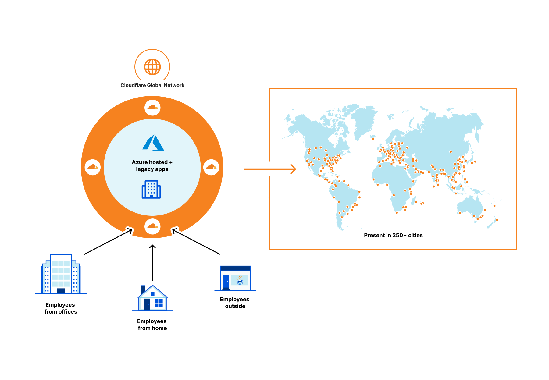
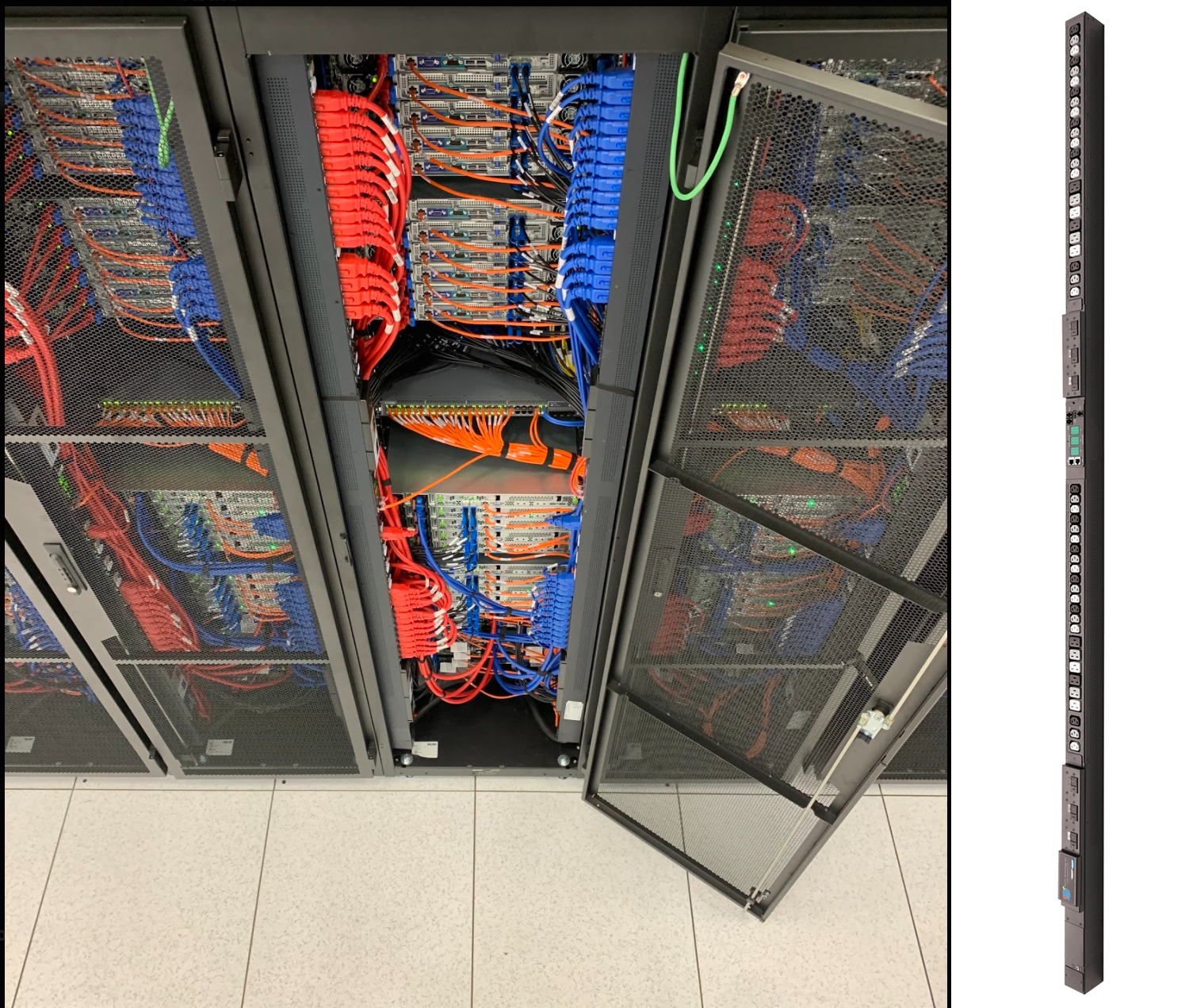
At Cloudflare we pride ourselves in our global network that spans more than 200 cities in over 100 countries. To handle all the traffic passing through our network, there are multiple technologies at play. So let’s have a look at one of the cornerstones that makes all of this work… ASICs. No, not the running shoes.

What’s an ASIC?

ASIC stands for Application Specific Integrated Circuit. The name already says it, it’s a chip with a very narrow use case, geared towards a single application. This is in stark contrast to a CPU (Central Processing Unit), or even a GPU (Graphics Processing Unit). A CPU is designed and built for general purpose computation, and does a lot of things reasonably well. A GPU is more geared towards graphics (it’s in the name), but in the last 15 years, there’s been a drastic shift towards GPGPU (General Purpose GPU), in which technologies such as CUDA or OpenCL allow you to use the highly parallel nature of the GPU to do general purpose computing. A good example of GPU use is video encoding, or more recently, computer vision, used in applications such as self-driving cars.

Unlike CPUs or GPUs, ASICs are built with a single function in mind. Great examples are the Google Tensor Processing Units (TPU), used to accelerate machine learning functions^[1], or for orbital maneuvering^[2], in which specific orbital maneuvers are encoded, like the Hohmann Transfer, used to move rockets (and their payloads) to a new orbit at a different altitude. And they are also heavily used in the networking industry. Technically, the use case in the network industry should be called an ASSP (Application Specific Standard Product), but network engineers are simple people, so we prefer to call it an ASIC.

Why an ASIC

ASICs have the major benefit of being hyper-efficient. The more complex hardware is, the more it will need cooling and power. As ASICs only contain the hardware components needed for their function, their overall size can be reduced, and so are their power requirements. This has a positive impact on the overall physical size of the network (devices don’t need to be as bulky to provide sufficient cooling), and helps reduce the power consumption of a data center.

Reducing hardware complexity also reduces the failure rate of the manufacturing process, and allows for easier production.

The downside is that you need to embed a lot of your features in hardware, and once a new technology or specification comes around, any chips made without that technology baked in, won’t be able to support it (VXLAN for example).

For network equipment, this works perfectly. Overall, the networking industry is slow-moving, and considerable time is taken before new technologies make it to the market (as can be seen with IPv6, MPLS implementations, xDSL availability, …). This means the chips don’t need to evolve on a yearly basis, and can instead be created on a much slower cycle, with bigger leaps in technology. For example, it took Broadcom two years to go from Tomahawk 3 to Tomahawk 4, but in that process they doubled the throughput. The benefits listed earlier are super helpful for network equipment, as they allow for considerable throughput in a small form factor.

Building an ASIC

As with chips of any kind, building an ASIC is a long-term process. Just like with CPUs, if there’s a defect in the hardware design, you have to start from scratch, and scrap the entire build line. As such, the development lifecycle is incredibly long. It starts with prototyping in an FPGA (Field Programmable Gate Array), in which chip designers can program their required functionality and confirm compatibility. All of this is done in a HDL (Hardware Description Language), such as Verilog.

Once the prototyping stage is over, they move to baking the new packet processing pipeline into the chip at a foundry. After that, no more changes can be made to the chip, as it’s literally baked into the hardware (unlike an FPGA, which can be reprogrammed). Further difficulty is added by the fact that there are a very small number of hardware companies that will buy ASICs in bulk to build equipment with; as such the unit cost can increase drastically.

All of this means that the iteration cycle of an ASIC tends to be on the slower side of things (compared to the yearly refreshes in the Intel Process-Architecture-Optimization model for example), and will usually be smaller incremental updates: For example, increases in port-speeds are incremental (1G → 10G → 25G → 40G → 100G → 400G → 800G → …), and are tied into upgrades to the SerDes (Serialiser/Deserialiser) part of the chip.

New protocol support is a lot harder, and might require multiple development cycles before it shows up in a chip.

What ASICs do

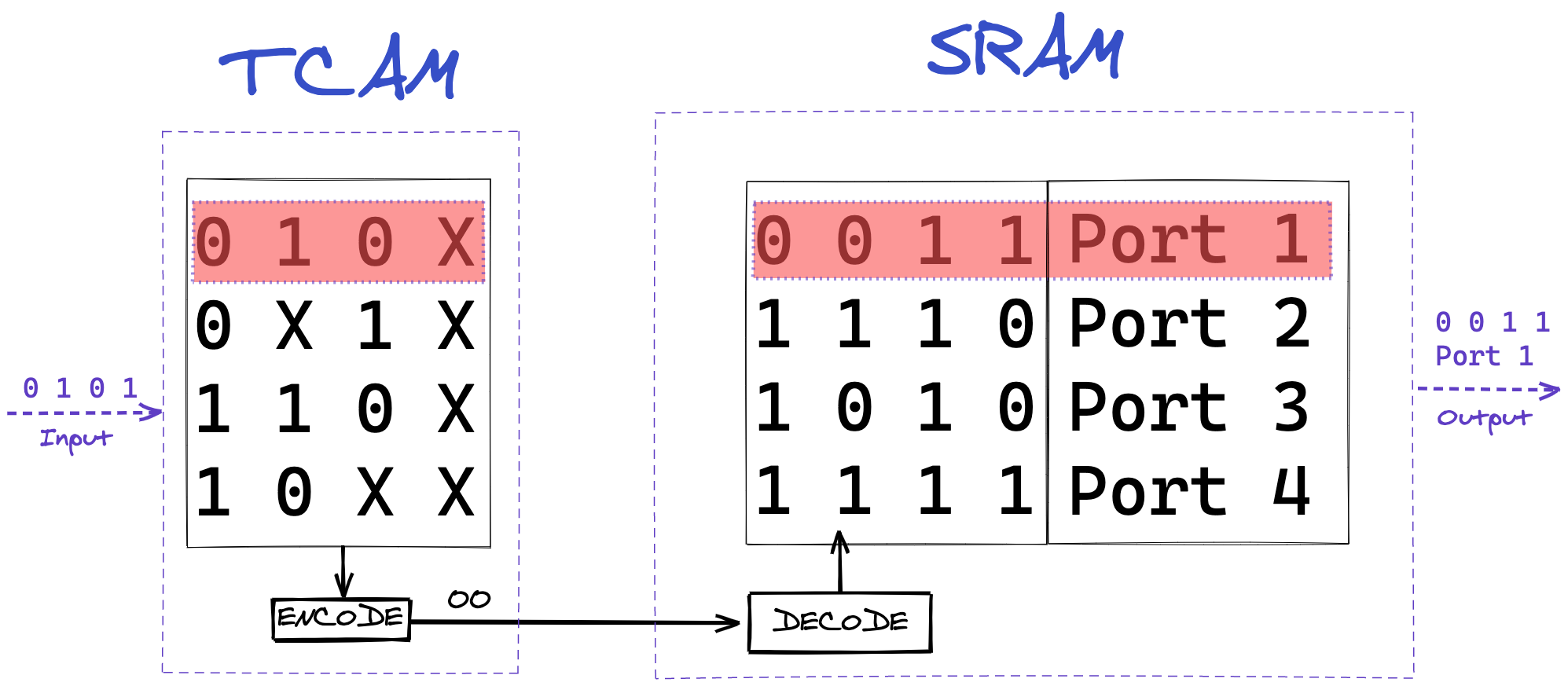
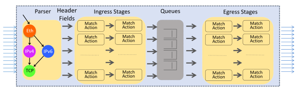
The ASICs in our network equipment are responsible for the switching and routing of packets, as well as being the first layer of defense (in the form of a stateless firewall). Due to the sheer nature of how fast packets get switched, fast memory access is a primary concern. Most ASICs will use a special sort of memory, called TCAM (Ternary Content-Addressable Memory). This memory will be used to store all sorts of lookup tables. These may be forwarding tables (where does this packet go), ACL (Access Control List) tables (is this packet allowed), or CoS (Class of Service) tables (which priority should be given to this packet)

CAM, and its more advanced sibling, TCAM, are fascinating kinds of memory, as they operate fundamentally different than traditional Random Access Memory (RAM). While you have to use a memory address to access data in RAM, with CAM and TCAM you can directly refer to the content you are looking for. It is a physical implementation of a key-value store.

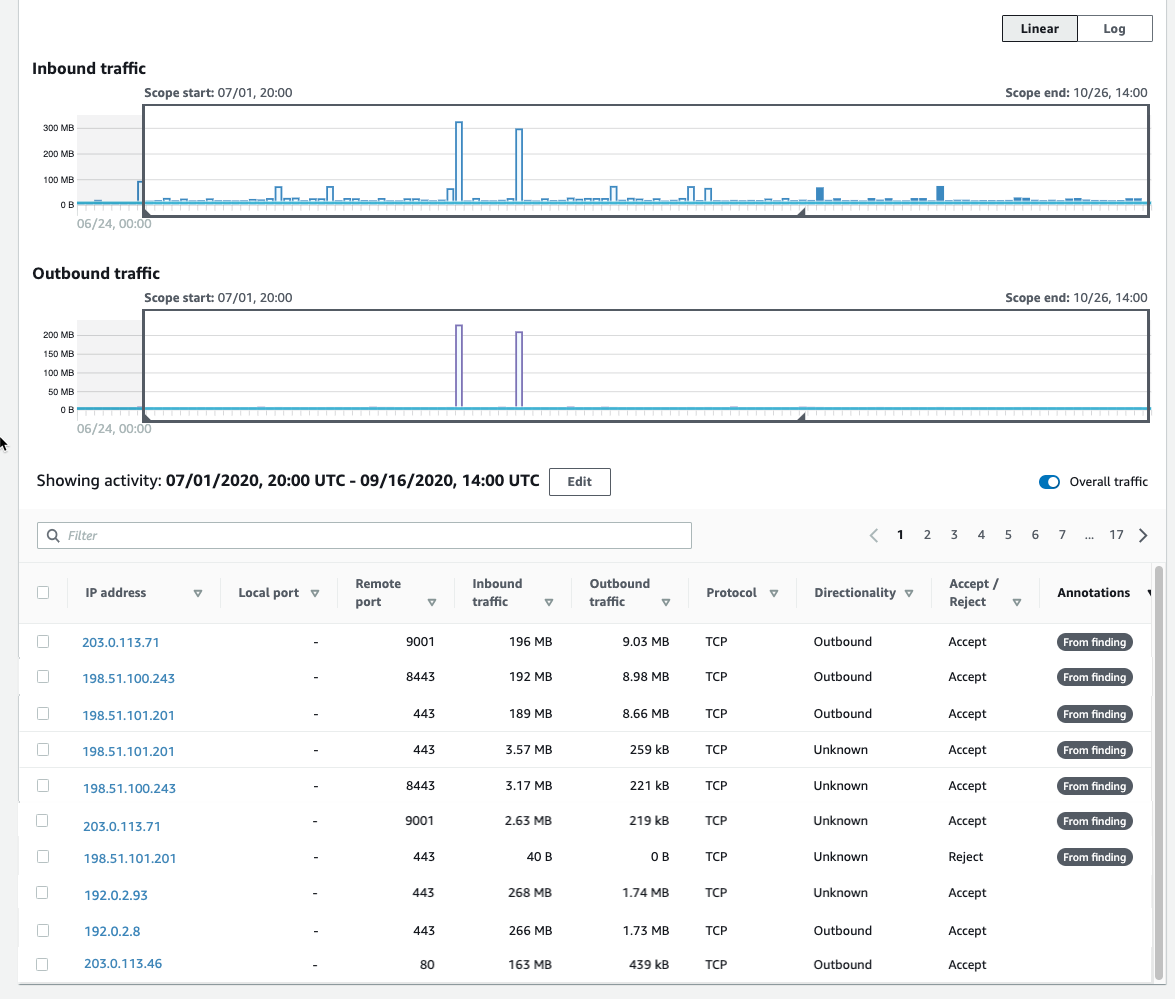
In CAM you use the exact binary representation of a word, in a network application, that word is likely going to be an IP address, so 11001011.00000000.01110001.00000000 for example (203.0.113.0). While this is definitely useful, networks operate a big collection of IP addresses, and storing each individually would require significant memory. To remedy this memory requirement, TCAM can store three states, instead of the binary two. This third state, sometimes called ‘ignore’ state, allows for the storage of multiple sequential data words as a single entry.

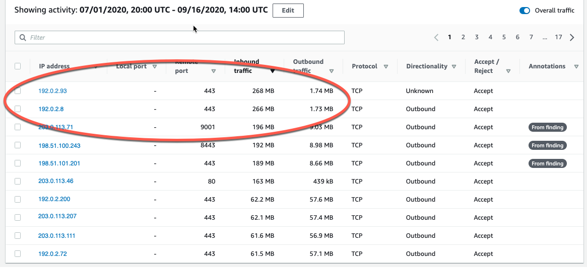
In networking, these sequential data words are IP prefixes. So for the previous example, if we wanted to store the collection of that IP address, and the 254 IPs following it, in TCAM it would as follows: 11001011.00000000.01110001.XXXXXXXX (203.0.113.0/24). This storage method means we can ask questions of the ASIC such as “where should I send packets with the destination IP address of 203.0.113.19”, to which the ASIC can have a reply ready in a single clock cycle, as it does not need to run through all memory, but instead can directly reference the key. This reply will usually be a reference to a memory address in traditional RAM, where more data can be stored, such as output port, or firewall requirements for the packet.

To dig a bit deeper into what ASICs do in network equipment, let’s briefly go over some fundamentals.

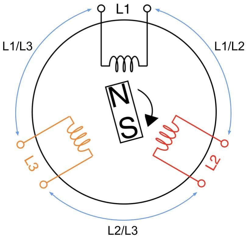
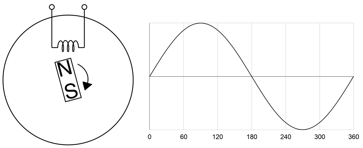
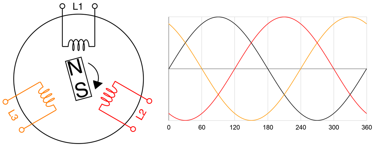
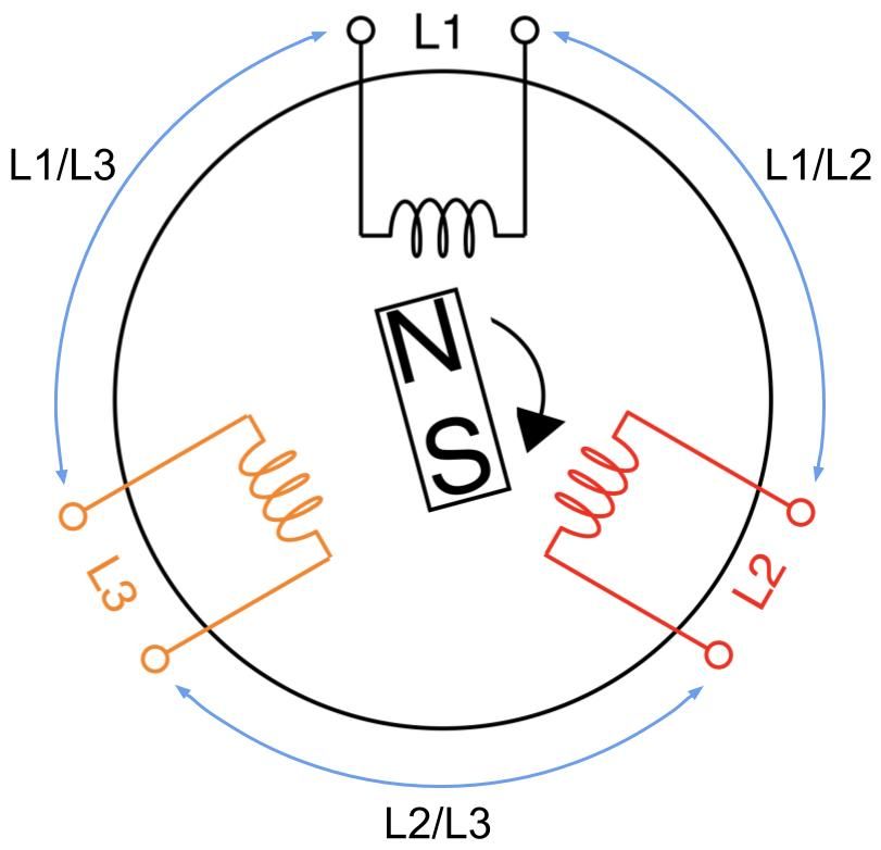
Networking can be split into two primary components: routing and switching. Switching allows you to directly interconnect multiple devices, so they can talk with each other across the network. It’s what allows your phone to connect to your TV to play a new family video. Routing is the next level up. It’s the mechanism that interconnects all these switched networks into a network of networks, and eventually, the Internet.

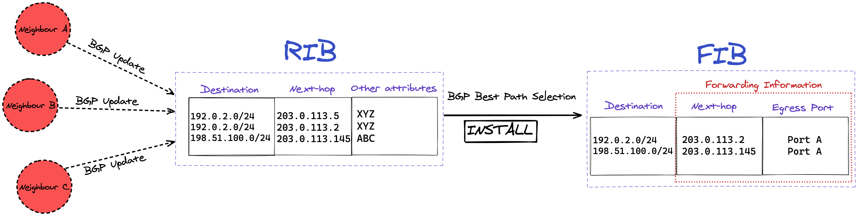
So routers are the devices responsible for steering traffic through this complex maze of networks, so it gets to its destination safely, and hopefully, as fast as possible. On the Internet, routers will usually use a routing protocol called BGP (Border Gateway Protocol) to exchange reachability information for a prefix (a collection of IP addresses), also called NLRI (Network Layer Reachability Information).

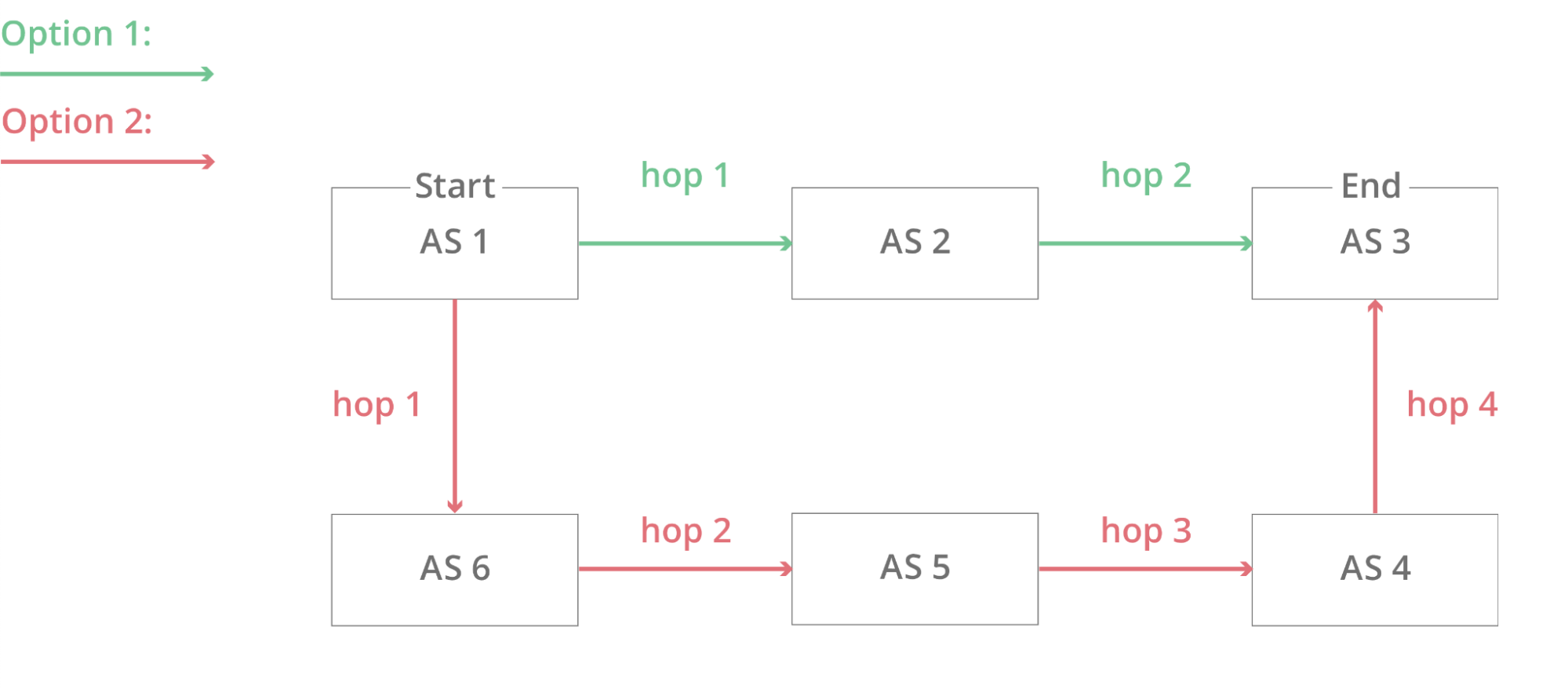
As with navigating the roads, there are multiple ways to get from point A to point B on the Internet. To make sure the router makes the right decision, it will store all of the reachability information in the RIB (Routing Information Base). That way, if anything changes with one route, the router still has other options immediately available.

With this information, a BGP daemon can calculate the ideal path to take for any given destination from its own point-of-view. This Cisco documentation explains the decision process the daemon goes through to calculate that ideal path.

Once we have this ideal path for a given destination, we should store this information, as it would be very inefficient to calculate this every single time we need to go there. The storage database is called the FIB (Forwarding Information Base). The FIB will be a subset of the RIB, as it will only ever contain the best path for a destination at any given time, while the RIB keeps all the available paths, even the non-ideal ones.

With these individual components, routers can make packets go from point A to point B in a blink of an eye.

Here’ are some of the more specific functions our ASICs need to perform:

1. FIB install: Once the router has calculated its FIB, it’s important the router can access this as quickly as possible. To do so, the ASIC will install (write) this calculated FIB into the TCAM, so any lookups can happen as quickly as possible.
   

2. Packet forwarding lookups: as we need to know where to send a received packet, we look up this information in TCAM, which is, as we mentioned, incredibly fast.

3. Stateless Firewall: while a router routes packets between destinations, you also want to ensure that certain packets don’t reach a destination at all. This can be done using either a stateless or stateful firewall. “State” in this case refers to TCP state, so the router would need to understand if a connection is new, or already established. As maintaining state is a complex issue, which requires storing tables, and can quickly consume a lot of memory, most routers will only operate a stateless firewall.
   Instead, stateful firewalls often have their own appliances. At Cloudflare, we’ve opted to move maintaining state to our compute nodes, as that severely reduces the state-table (one router for all state vs X metals for all state combined). A stateless firewall makes use of the TCAM again to store rules on what to do with specific types of packets. For example, one of the rules we employ at our edge is DENY-BOGON-RANGES , in which we discard traffic sourced from RFC1918 space (and other unroutable space). As this makes use of TCAM, it can all be done at line rate (the maximum speed of the interface).

4. Advanced features, such as GRE encapsulation: modern networking isn’t just packet switching and packet routing anymore, and more advanced features are needed. One of these is encapsulation. With packet encapsulation, a system will put a data packet into another data packet. Using this technique, it’s possible to build a network on top of an existing network (an overlay). Overlays can be used to build a virtual backbone for example, in which multiple locations can be virtually connected through the Internet.
   While you can encapsulate packets on a CPU (we do this for Magic Transit), there are considerable challenges in doing so in software. As such, the ASIC can have built-in functionality to encapsulate a packet in a multitude of protocols, such as GRE. You may not want encapsulated packets to have to take a second trip through your entire pipeline, as this adds latency, so these shortcuts can also be built into the chip.

5. MPLS, EVPN, VXLAN, SDWAN, SDN, …: I ran out of buzzwords to enumerate here, but while MPLS isn’t new (the first RFC was created in 2001), it’s a rather advanced requirement, just as the others listed, which means not all ASIC vendors will implement this for all their chips due to the increased complexity.

Vendor Landscape

At Cloudflare, we interact with both hardware and software vendors on a daily basis while operating our global network. As we’re talking about ASICs today, we’ll explore the hardware landscape, but some hardware vendors also have their own NOS (Network Operating System).
There’s a vast selection of hardware out there, all with different features and pricing. It can become incredibly hard to see the wood for the trees, so we’ll focus on 4 important distinguishing factors: Throughput (how many bits can the ASIC push through), buffer size (how many bits can the ASIC store in memory in case of resource contention), programmability (how easy is it for a third party programmer like Cloudflare to interact directly with the ASIC), feature set (how many advanced things outside of routing/switching can the ASIC do).

The landscape is so varied because different companies have different requirements. A company like Cloudflare has different expectations for its network hardware than your typical corner shop. Even within our own network we’ll have different requirements for the different layers that make up our network.

Broadcom

The elephant in the networking room (or is it the jumbo frame in the switch?) is Broadcom. Broadcom is a semiconductor company, with their primary revenue in the wired infrastructure segment (over 50% of revenue^[3]). While they’ve been around since 1991, they’ve become an unstoppable force in the last 10 years, in part due to their reliance on Apple (25% of revenue). As a semiconductor manufacturer, their market dominance is primarily achieved by acquiring other companies. A great example is the acquisition of Dune Networks, which has become an excellent revenue generator as the StrataDNX series of ASIC (Arad, QumranMX, Jericho). As such, they have become the biggest ASIC vendor by far, and own 59% of the entire Ethernet Integrated Circuits market^[4].

As such, they supply a lot of merchant silicon to Cisco, Juniper, Arista and others. Up until recently, if you wanted to use the Broadcom SDK to accelerate your packet forwarding, you have to sign so many NDAs you might get a hand cramp, which makes programming them a lot trickier. This changed recently when Broadcom open-sourced their SDK. Let’s have a quick look at some of their products.

Tomahawk

The Tomahawk line of ASICs are the bread-and-butter for the enterprise market. They’re cheap and incredibly fast. The first generation of Tomahawk chips did 3.2Tbps linerate, with low-latency switching. The latest generation of this chip (Tomahawk 4) does 25.6Tbps in a 7nm transistor footprint^[5]). As you can’t have a cheap, fast, and full feature set for a single package, this means you lose out on features. In this case, you’re missing most of the more advanced networking technologies such as VXLAN, and you have no buffer to speak of.
As an example of a different vendor using this silicon, you can have a look at the Juniper QFX5200 switching platform.

StrataDNX (Arad, QumranMX, Jericho)

These chipsets came through the acquisition of Dune Networks, and are a collection of high-bandwidth, deep buffer (large amount of memory available to store (buffer) packets) chips, allowing them to be deployed in versatile environments, including the Cloudflare edge. The Arista DCS-7280SR that we run in some of our edge locations as edge routers run on the Jericho chipset. Since then, the chips have evolved, and with Jericho2, Broadcom now have a 10Tbps deep buffer chip^[6]. With their fabric chip (this links multiple ASICs together), you can build switches with 48x400G ports^[7] without much effort.
Cisco built their NCS5500 line of routers using the QumranMX^[8].

Trident

This ASIC is an upgrade from the Tomahawk chipset, with a complex and extensive feature set, while maintaining high throughput rates. The latest Trident4 does 12.8Tbps at incredibly low latencies^[9], making it an incredibly flexible platform. It unfortunately has no buffer space to speak of, which limits its scope for Cloudflare, as we need the buffer space to be able to switch between the different port speeds we have on our edge routers. The Arista 7050X and 7300X are built on top of this.

Intel

Intel is well known in the network industry for building stable and high-performance 10G NICs (Network Interface Controller). They’re not known for ASICs. They made an initial attempt with their acquisition of Fulcrum^[10], which built the FM6000^[11] series of ASIC, but nothing of note was really built with them. Intel decided to try again in 2019 with their acquisition of Barefoot. This small manufacturer is responsible for the Barefoot Tofino ASIC, which may well be a fundamental paradigm shift in the network industry.

Barefoot Tofino

The Tofino^[12] is built using a PISA (Protocol Independent Switch Architecture), and using P4 (Programming Protocol-Independent Packet Processors)^[13], you can program the data-plane (packet forwarding) as you see fit. It’s a drastic move away from the traditional method of networking, in which direct programming of the ASIC isn’t easily possible, and definitely not through a standard programming language. As an added benefit, P4 also allows you to perform a formal verification of your forwarding program, and be sure that it will do what you expect it to. Caveat: OpenFlow tried this, but unfortunately never really got much traction.
^[14]

There are multiple variations of the Tofino 1 available, but the top-end ASIC has a 6.5Tbps linerate capacity. As the ASIC is programmable, its featureset is as rich as you’d want it to be. Unfortunately, the chip does not come with a lot of buffer memory, so we can’t deploy these as edge devices (yet). Both Arista (7170 Series^[15]) and Cisco (Nexus 34180YC and 3464C series^[16]) have built equipment with the Tofino chip inside.

Mellanox

As some of you may know, Mellanox is the vendor that recently got acquired by Nvidia, which also provides our 25G NICs in our compute nodes. Besides NICs, Mellanox has a well-established line of ASICs, mostly for switching.

Spectrum

The latest iteration of this ASIC, Spectrum 3 offers 12.8Tbps switching capacity, with an extensive featureset, including Deep Packet Inspection and NAT. This chip allows for building dense high-speed port devices, going up to 25.6Tbps^[17]. Buffering wise, there’s none to really speak of (64MB). Mellanox also builds their own hardware platforms. Unlike the other vendors below, they aren’t shipped with the Mellanox Operating System, instead, they offer you a variety of choices to run on top, including Cumulus Linux (which was also acquired by Nvidia 🤔).

As mentioned, while we use their NIC technology extensively, we currently don’t have any Mellanox ASIC silicon in our network.

Juniper

Juniper is a network hardware supplier, and currently the biggest supplier of network equipment for Cloudflare. As previously mentioned in the Broadcom section, Juniper buys some of their silicon from Broadcom, but they also have a significant lineup of home-grown silicon, which can be split into 2 families: Trio and Express.

Express

The Express family is the switching-skewed family, where bandwidth is a priority, while still maintaining a broad range of feature capabilities. These chips live in the same application landscape as the Broadcom StrataDNX chips.

Paradise (Q5)

The Q5 is the new generation of the Juniper switching ASIC^[18]. While by itself it doesn’t boast high linerates (500Gbps), when combined into a chassis with a fabric chip (Clos network in this case), they can produce switches (or line cards) with up to 12Tbps of throughput capacity^[19]. In addition to allowing for high-throughput, dense network appliances, the chip also comes with a staggering amount of buffer space (4GB per ASIC), provided by external HMC (Hybrid Memory Cube). In this HMC, they’ve also decided to put the FIB, MAC and other tables (so no TCAM).
The Q5 chip is used in their QFX1000 lineup of switches, which include the QFX10002-36Q, QFX10002-60C, QFX10002-72Q and QFX10008, all of which are deployed in our datacenters, as either edge routers or core aggregation switches.

ExpressPlus (ZX)

The ExpressPlus is the more feature-rich and faster evolution of the Paradise chip. It offers double the bandwidth per chip (1Tbps) and is built into a combined Clos-fabric reaching 6Tbps in a 2U form-factor (PTX10002). It also has an increased logical scale, which comes with bigger buffers, larger FIB storage, and more ACL space.

The ExpressPlus drives some of the PTX line of IP routers, together with its newest sibling, Triton.

Triton (BT)

Triton is the latest generation of ASIC in the Express family, with 3.6Tbps of capacity per chip, making way for some truly bandwidth-dense hardware. Both Triton and ExpressPlus are 400GE capable.

Trio

The Trio family of chips are primarily used in the feature-heavy MX routing platform, and is currently at its 5th generation.

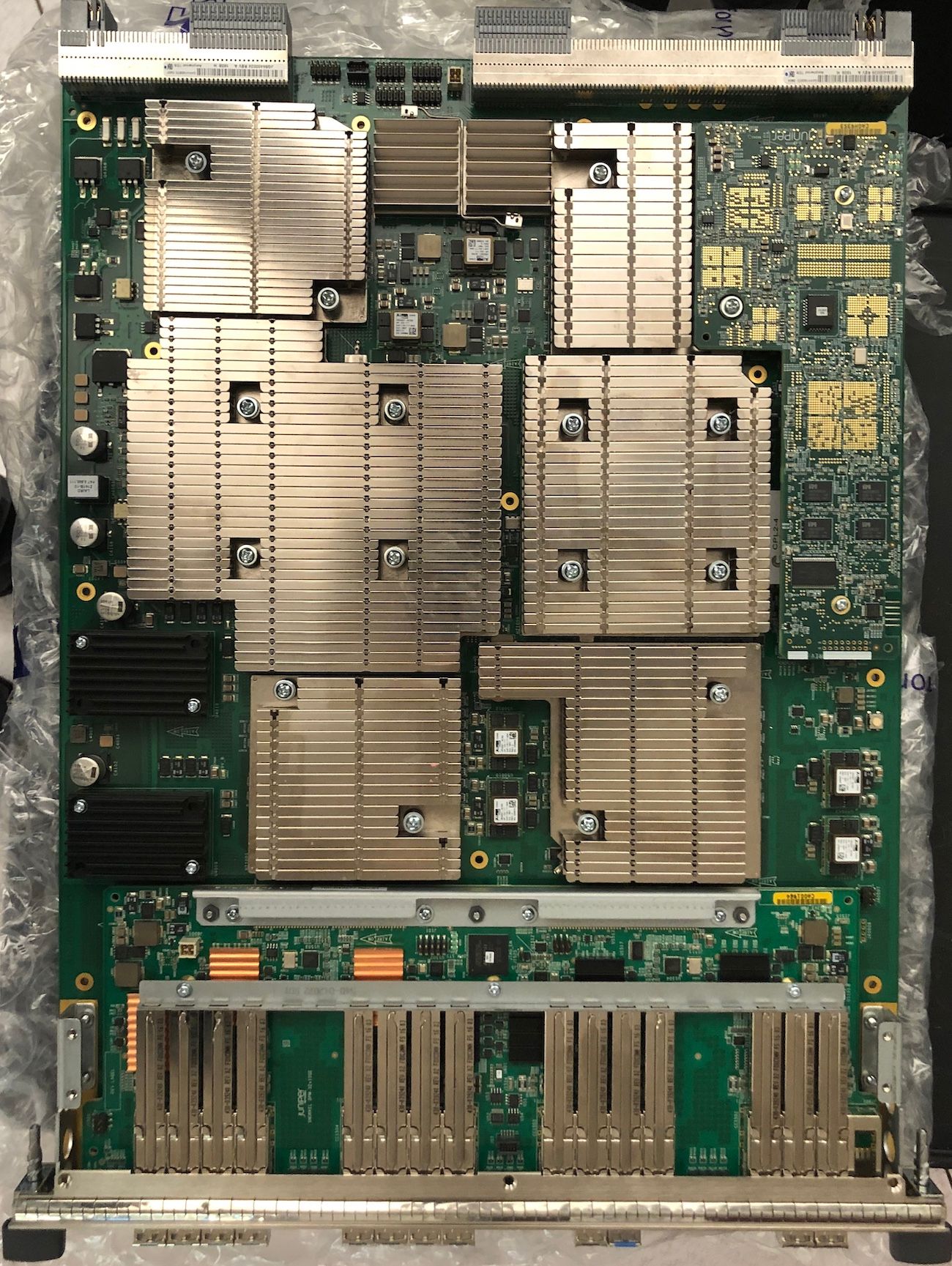
A Juniper MPC4E-3D-32XGE line card

Trio Eagle (Trio 4.0) (EA)

The Trio Eagle is the previous generation of the Trio Penta, and can be found on the MPC7E line cards for example. It’s a feature-rich ASIC, with a 400Gbps forwarding capacity, and significant buffer and TCAM capacity (as is to be expected from a routing platform ASIC)

Trio Penta (Trio 5.0) (ZT)

Penta is the new generation routing chip, which is built for the MX platform routers. On top of being a very beefy chip, capable of 500Gbps per ASIC, allowing Juniper to build line cards of up to 4Tbps of capacity, the chip also has a lot of baked in features, offering advanced hardware offloading for for example MACSec, or Layer 3 IPsec.

The Penta chip is packaged on the MPC10E and MPC11E line card, which can be installed in multiple variations of the MX chassis routers (MX480 included).

Cisco

Last but not least, there’s Cisco. As the saying goes “nobody ever got fired for buying Cisco”, they’re the biggest vendor of network solutions around. Just like Juniper, they have a mixed product fleet of merchant silicon, as well as home-grown. While we used to operate Cisco routers as edge routers (Cisco ASR 9000), this is no longer the case. We do still use them heavily for our ToR (Top-of-Rack) switching needs, utilizing both their Nexus 5000 series and Nexus 9000 series switches.

Bigsur

Bigsur is custom silicon developed for the Nexus 6000 line of switches (confusingly, the switches themselves are called Cisco Nexus 5672UP and Cisco Nexus 6001). In our specific model, the Cisco Nexus 5672UP, there’s 7 of them interconnected, providing 10G and 40G connectivity. Unfortunately Cisco is a lot more tight-lipped about their ASIC capabilities, so I can’t go as deep as I did with the Juniper chips. Feature-wise, there’s not a lot we require from them in our edge network. They’re simple Layer 2 forwarding switches, with no added requirements. Buffer wise, they use a system called Virtual Output Queueing, just like the Juniper Express chip. Unlike the Juniper silicon, the Bigsur ASIC doesn’t come with a lot of TCAM or buffer space.

Tahoe

The Tahoe is the Cisco ASIC found in the Cisco 9300-EX switches, also known as the LSE (Leaf Spine Engine). It offers higher-density port configurations compared to the Bigsur (1.6Tbps)^[20]. Overall, this ASIC is a maturation of the Bigsur silicon, offering more advanced features such as advanced VXLAN+EVPN fabrics, greater port flexibility (10G, 25G, 40G and 100G), and increased buffer sizes (40MB). We use this ASIC extensively in both our edge data centers as well as in our core data centers.

Conclusion

A lot of different factors come into play when making the decision to purchase the next generation of Cloudflare network equipment. This post only scratches the surface of technical considerations to be made, and doesn’t come near any other factors, such as ecosystem contributions, openness, interoperability, or pricing. None of this would’ve been possible without the contributions from other network engineers—this post was written on the shoulders of giants. In particular, thanks to the excellent work by Jim Warner at UCSC, the engrossing book on the new MX platforms, written by David Roy (Day One: Inside the MX 5G), as well as the best book on the Juniper QFX lineup: Juniper QFX10000 Series by Douglas Richard Hanks Jr, and to finish it off, the Summary of Network ASICs post by Justin Pietsch.