Post Syndicated from Swara Gandhi original https://aws.amazon.com/blogs/security/how-to-prioritize-iam-access-analyzer-findings/
AWS Identity and Access Management (IAM) Access Analyzer is an important tool in your journey towards least privilege access. You can use IAM Access Analyzer access previews to preview and validate public and cross-account access before deploying permissions changes in your environment.
For the permissions already in place, one of IAM Access Analyzer’s capabilities is that it helps you identify resources in your AWS Organizations organization and AWS accounts that are shared with an external entity.
For each external entity that has access to a resource in your account, IAM Access Analyzer generates a finding. Findings display information about the resource and the policy statement that generated the finding, with details such as the list of actions in the policy granting access, level of access, and conditions that allow the access. You can review the findings to determine if the access is intended or unintended.
As your use of AWS services grows and the number of accounts in your organization increases, the number of findings that you have might also increase. To help reduce noise and allow you to focus on unintended access findings, you can filter findings and create archive rules for intended access.
This blog post provides step-by-step guidance on how to get started with IAM Access Analyzer findings by using different filtering techniques that can help you filter approved use cases that result in access findings. For example, you might see a finding generated for an S3 bucket that hosts images for your website and thus allows public access, as approved by your organization, apply a filter so that you can concentrate on unintended access. IAM Access Analyzer offers a wide range of filters; for a complete list, see the IAM documentation.
In this post, we also share example archive rules for approved use cases that result in access findings. Archive rules automatically archive new findings that meet the criteria you define when you create the rule. You can also apply archive rules retroactively to archive existing findings that meet the archive rule criteria. Finally, we have included an example implementation of archive rules using an AWS CloudFormation template.
IAM Access Analyzer findings overview
To get started, create an analyzer for your entire organization or your account. The organization or account that you choose is known as the zone of trust for the analyzer. The zone of trust determines the type of access that IAM Access Analyzer considers to be trusted. IAM Access Analyzer continuously monitors to identify resource policies, access control lists, and other access controls that grant public or cross-account access from outside the zone of trust, and generates findings. For this blog post, we’ll demonstrate an organization as the zone of trust, showcasing findings from a large-scale, multi-account AWS deployment.
Prerequisites
This blog post assumes that you have the following in place:
- IAM Access Analyzer is enabled in your organization or account in the AWS Regions where you operate. For more details on how to enable IAM Access Analyzer, see Enabling IAM Access Analyzer.
- Access to the AWS Organizations management account or to a member account in the organization with delegated administrator access for creating and updating IAM Access Analyzer resources.
How to filter the findings
To start filtering your findings and create archive rules, you should complete the following steps:
- Review public access findings
- Filter by removing permissions errors
- Filter for known identity providers
- Filter cross-account access from trusted external accounts
We’ll walk you through each step.
1. Review public access findings
Some AWS resources allow public access on the resource by means of a resource-based policy—for example, an Amazon Simple Storage Service (Amazon S3) bucket policy that has the “Principal:*” permission added to its bucket policy. For resources such as Amazon Elastic Block Store (Amazon EBS) snapshots, you can share these by using a flag on the resource permission. IAM Access Analyzer looks for such sharing and reports it in the findings.
From the global report, you can generate a list of resources that allow public access by using the Public access: true query in the IAM console.
The following is an example of an AWS Command Line Interface (AWS CLI) command with public access as “true”. Replace <AccessAnalyzerARN> with the Amazon Resource Name (ARN) of your analyzer.
aws accessanalyzer list-findings --analyzer-arn <AccessAnalyzerARN> --filter isPublic={"eq"="true"}
Is the public access intended?
If the access is intended, you can archive the findings by creating an archive rule using the AWS Management Console, AWS CLI, or API. When you archive a security finding, IAM Access Analyzer removes it from the Active findings list and changes its status to Archived. For instructions on how to automatically archive expected findings, see How to automatically archive expected IAM Access Analyzer findings.
Example: Known S3 bucket that hosts public website images
If you have resources for which public access is expected, such as an S3 bucket that hosts images for your website, you can add an archive rule with Resource criteria equal to the bucket name, as shown in Figure 1.
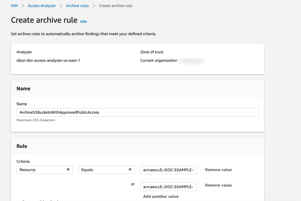
Figure 1: Create IAM Access Analyzer archive rule using the console
Is the public access unintended?
If the finding results from policies that were misconfigured to allow unintended public access, you can constrain the access by using AWS global condition context keys or a specific IAM principal ARN. The findings show the account and resource that contain the policy.
For example, if the finding shows a misconfigured S3 bucket, the following policy shows how you can modify the S3 bucket policy to only allow IAM principals from your organization to access the bucket by using the PrincipalOrgID condition key. Replace <DOC-EXAMPLE-BUCKET> with the name of your S3 bucket, and <ORGANIZATION_ID> with your organization ID.
2. Filter by removing permissions errors
Before you further investigate the IAM Access Analyzer findings, you should make sure that IAM Access Analyzer has enough permissions to access the resources in your accounts to be able to provide the analysis.
IAM Access Analyzer uses an AWS service-linked role to call other AWS services on your behalf. When IAM Access Analyzer analyzes a resource, it reads resource metadata, such as a resource-based policy, access control lists, and other access controls that grant public or cross-account access. If the policies don’t allow an IAM Access Analyzer role to read the resource metadata, it generates an Access Denied error finding, as shown in Figure 2.
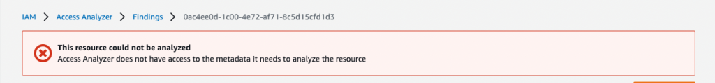
Figure 2: IAM Access Analyzer access denied error example
To view these error findings from the IAM Access Analyzer console, filter the findings by using the Error: Access Denied property.
Resolution
To resolve the access issue, make sure that the IAM Access Analyzer service-linked role is not denied access. Review the resource-based policy attached to the resource that IAM Access Analyzer isn’t able to access. For a list of services that support resource-based policies, see the IAM documentation.
For example, if the analyzer can’t access an AWS Key Management Service (AWS KMS) key because of an explicit deny, add an exception for the IAM Access Analyzer service-linked role to the policy statement, similar to the following. Make sure that you change the <ACCOUNT_ID> to your account id.
| Before | After |
3. Filter for known identity providers
With SAML 2.0 or Open ID Connect (OIDC)—which are open federation standards that many identity providers (IdPs) use—users can log in to the console or call the AWS API operations without you having to create an IAM user for everyone in your organization.
To set up federation, you must perform a one-time configuration so that your organization’s IdP and your account trust each other. To configure this trust, you must register AWS as a service provider (SP) with the IdP of your organization and set up metadata and key exchange.
The role or roles that you create in IAM define what the federated users from your organization are allowed to use on AWS. When you create the trust policy for the role, you specify the SAML or OIDC provider as the Principal. To only allow users that match certain attributes to access the role, you can scope the trust policy with a Condition.
Example 1: Federation with Okta
Let’s walk through an example that uses Okta as the IdP. Although access to a trusted IdP is intended, IAM Access Analyzer creates a finding for an IAM role that has trust policy granting access to a SAML provider because the trust policy allows access outside of the known zone of trust for the analyzer. You will see findings created for the IAM role granting access to Okta using the IAM trust policy, as shown in Figure 3.
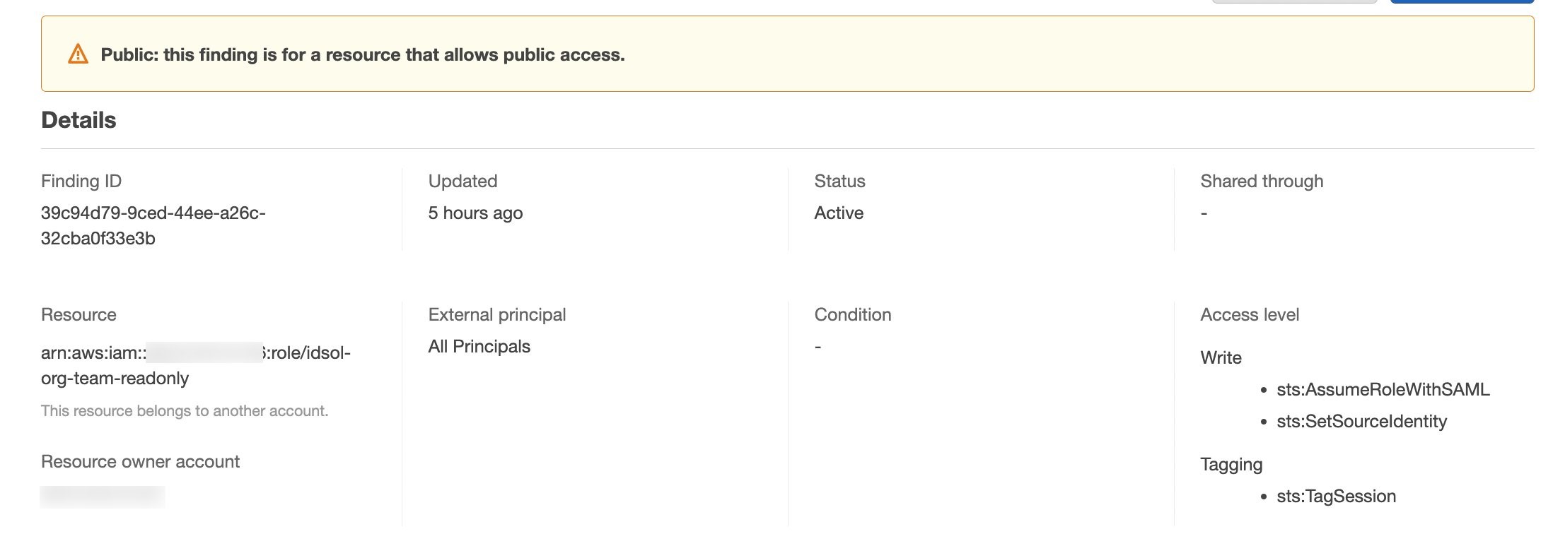
Figure 3: IAM Access Analyzer identity provider finding example
Resolution
Setting access through SAML providers is a privileged operation, so we recommend that you analyze each finding to decide if an exception is acceptable. If you approve of the SAML-provided access setup, you can implement an archive rule to archive such findings with conditions for federation used in combination with your SAML provider. The filter for the Federated User rule depends on the name that you gave to the SAML IdP in your federation setup. For example, if your SAML IdP name is Okta, the rule should have a filter for arn:aws:iam::<ACCOUNT_ID>:saml-provider/Okta, where <ACCOUNT_ID> is your account number, as shown in Figure 4.
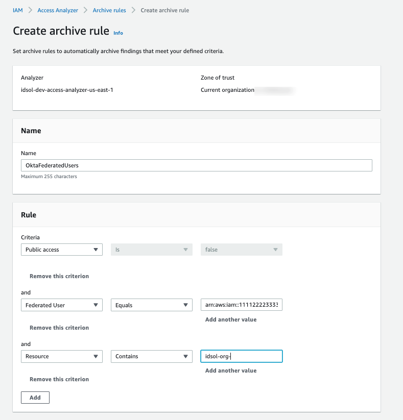
Figure 4: Archive rule example for using an IdP-related finding
Note: To include additional values for a multi-account setup, use the Add another value filter.
Example 2: IAM Identity Center
With AWS IAM Identity Center (successor to AWS Single Sign-On), you can manage sign-in security for your workforce. IAM Identity Center provides a central place to define your permission sets, assign them to your users and groups, and give your users a portal where they can access their assigned accounts.
With IAM Identity Center, you manage access to accounts by creating and assigning permission sets. These are IAM role templates that define (among other things) which policies to include in a role. When you create a permission set in IAM Identity Center and associate it to an account, IAM Identity Center creates a role in that account with a trust policy that allows a federated IdP as a principal — in this case, IAM Identity Center.
IAM Access Analyzer generates a finding for this setup because the allowed access is outside of the known zone of trust for the analyzer, as shown in Figure 5.
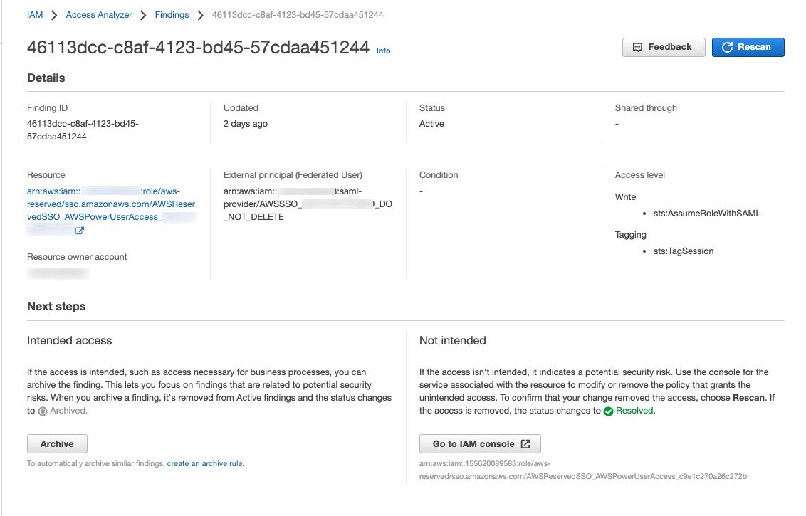
Figure 5: IAM Access Analyzer finding example for IAM Identity Center
To filter this finding, you need to implement an archive rule.
Resolution
You can implement an archive rule with conditions for federation used in combination with IAM Identity Center as the SAML provider. The roles created by IAM Identity Center in member accounts use a reserved path on AWS: arn:aws:iam::<ACCOUNT_ID>:role/aws-reserved/sso.amazonaws.com/. Hence, you can create an archive rule with a filter that contains :saml-provider/AWSSSO in the Federated User name and aws-reserved/sso.amazonaws.com/ in the Resource, as shown in Figure 6.
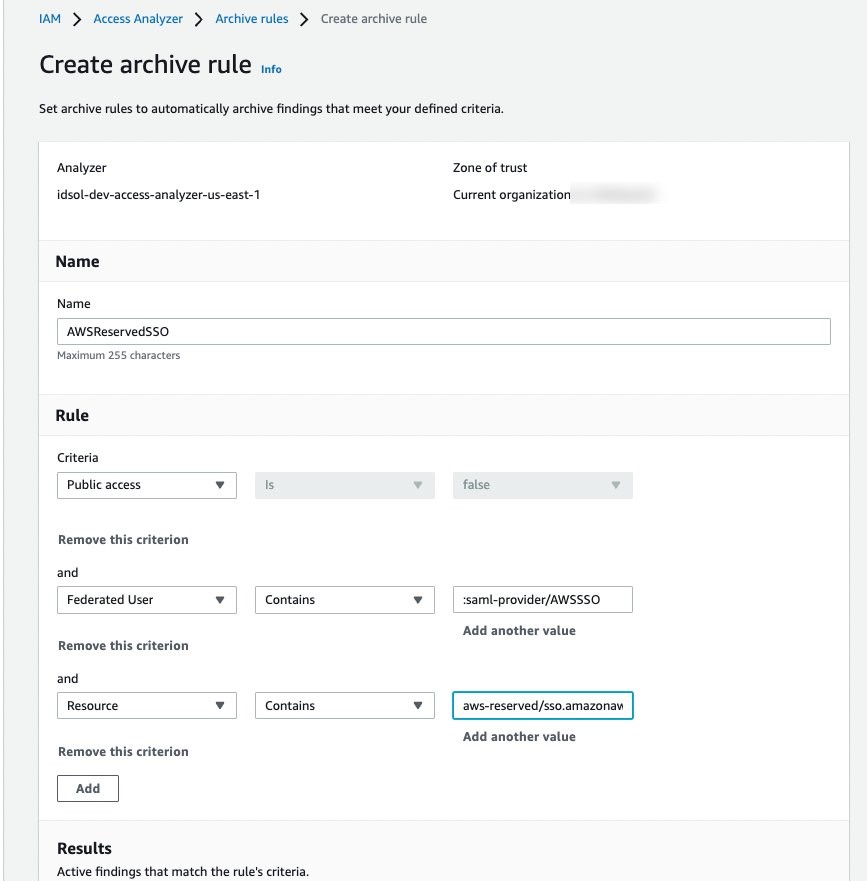
Figure 6: Archive rule example for IAM Identity Center generated findings
4. Filter cross-account access findings from trusted external accounts
We recommend that you identify and document accounts and principals that should be allowed access outside of the zone of trust for IAM Access Analyzer.
When a resource-based policy attached to a resource allows cross-account access from outside the zone of trust, IAM Access Analyzer generates cross-account access findings.
Is the cross-account access intended?
When you review cross-account access findings, you need to determine whether the access is intended or not. For example, you might have access provided to your auditor’s account or a partner account for visibility and monitoring of your AWS applications.
For trusted external accounts, you can create an archive rule that includes the AWS account in the criteria for the rule. Figure 7 shows an example of how to create the archive rule for a trusted external account (EXTERNAL_ACCOUNT_ID). In your own rule, replace EXTERNAL_ACCOUNT_ID with the trusted account id.
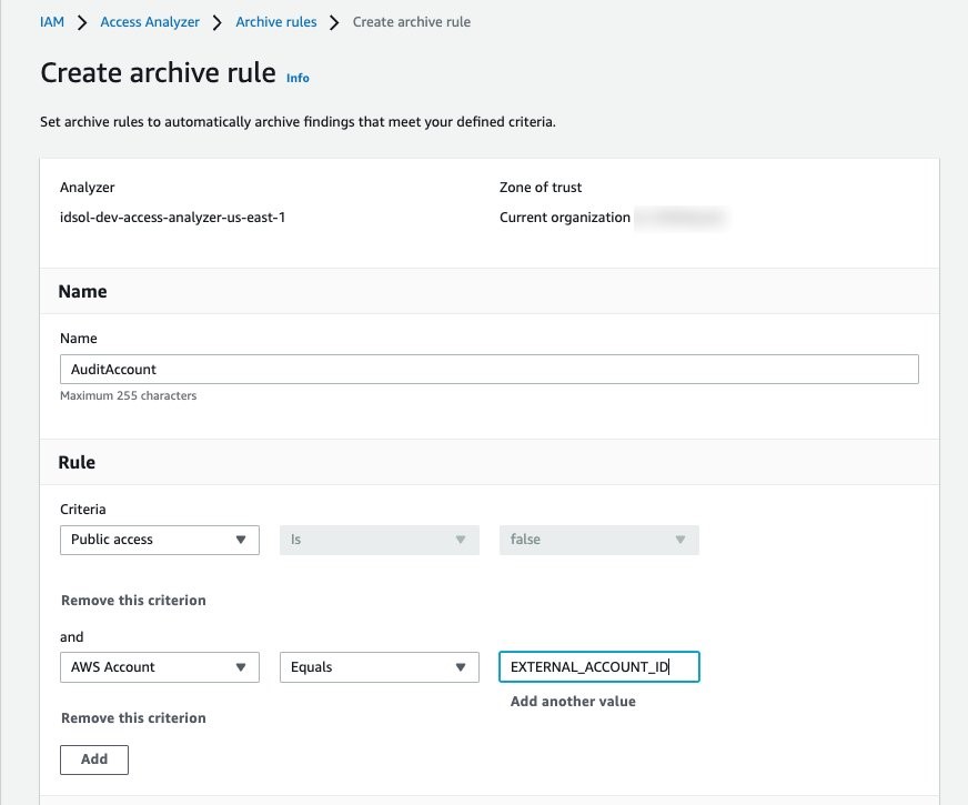
Figure 7: Archive rule example for trusted account findings
Is the cross-account access unintended?
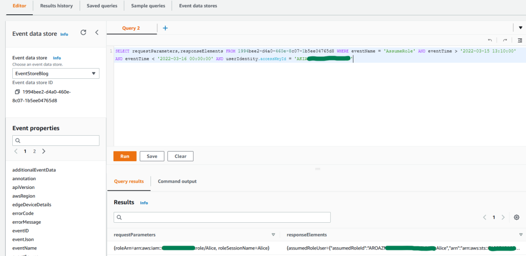
After you have archived the intended access findings, you can start analyzing the findings initiated from unintended access. When you confirm that the findings show unintended access, you should take steps to remove the access by altering or deleting the policy or access control that granted access. You can expand the solution outlined in the blog post Automate resolution for IAM Access Analyzer cross-account access findings on IAM roles by adding an explicit deny statement.
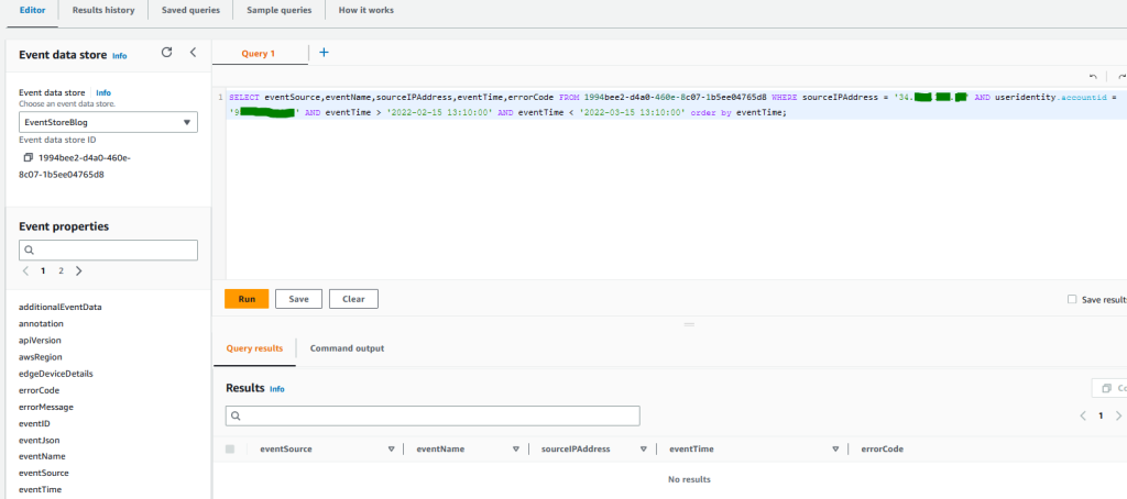
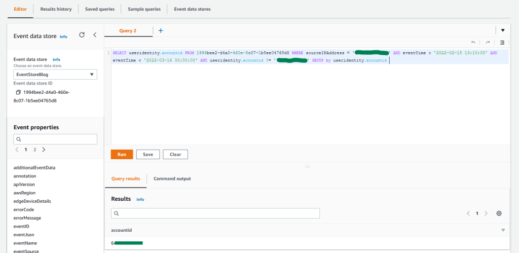
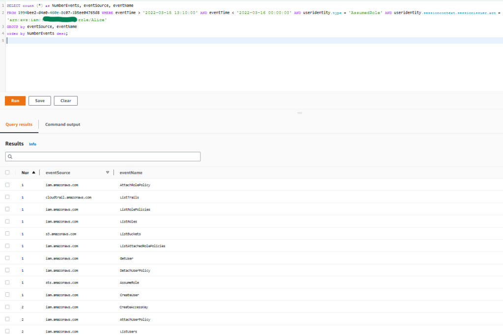
You can also use AWS CloudTrail to track API calls that could have changed access configuration on your AWS resources.
Deploy IAM Access Analyzer and archive rules with a CloudFormation template
In this section, we demonstrate a sample CloudFormation template that creates an IAM access analyzer and archive rules for findings that are created for identified intended access to resources.
Important: When you create an archive rule using the AWS console, the existing findings and new findings that match criteria mentioned in the rules will be archived. However, archive rules created through CloudFormation or the AWS CLI will only archive the new findings that meet the criteria defined. You need to perform the access-analyzer:ApplyArchiveRule API after you create the archive rule to archive existing findings as well.
The sample CloudFormation template takes the following values as inputs and creates archive rules for findings that are created for identified intended access to resources shared outside of your zone of trust for the specified analyzer:
- Analyzer name
- Zone of trust
- Known public S3 buckets, if you have any (for example, a bucket that hosts public website images).
Note: We use S3 buckets as an example. You can edit the rule to include resource types that are supported by IAM Access Analyzer, if public access is intended.
- Trusted accounts — AWS accounts that don’t belong to your organization, but you trust them to have access to resources in your organization
- SAML provider — The SAML provider approved to have access to your resources
Note: If you don’t use federation, you can remove the rule SAMLFederatedUsers.
AWSTemplateFormatVersion: 2010-09-09
Description: >+
  Sample CloudFormation template creates archive rules for findings
  created for resources shared outside of your zone of trust for specified
  analyzer.

Metadata:
  AWS::CloudFormation::Interface:
    ParameterGroups:
      - Label:
          default: Define Configuration
        Parameters:
          - AccessAnalyzerName
          - ZoneOfTrust
          - KnownPublicS3Buckets
          - TrustedAccounts
          - SAMLProvider
Parameters:
  AccessAnalyzerName:
    Description: Provide name of the analyzer you would like to create archive rules for.
    Type: String
  ZoneOfTrust:
    Description: Select the zone of trust of AccessAnalyzer
    AllowedValues:
      - ACCOUNT
      - ORGANIZATION
    Type: String
  KnownPublicS3Buckets:
    Description: List of comma-separated known S3 bucket arns, that should allow
      public access Example -
      arn:aws:s3:::DOC-EXAMPLE-BUCKET,arn:aws:s3:::DOC-EXAMPLE-BUCKET2
    Type: CommaDelimitedList
  TrustedAccounts:
    Description: List of comma-separated account IDs, that do not belong to your
      organization but you trust them to have access to resources in your
      organization. [Example - Your auditor’s AWS account]
    Type: List<Number>
  TrustedFederationPrincipals:
    Description: List of comma-separated trusted federated principals that are able
      to assume roles in your accounts. [Example -
      arn:aws:iam::012345678901:saml-provider/Okta,
      arn:aws:iam::1111222233334444:saml-provider/Okta]
    Type: CommaDelimitedList
Resources:
  AccessAnalyzer:
    Type: AWS::AccessAnalyzer::Analyzer
    Properties:
      AnalyzerName: ${AccessAnalyzerName}-${AWS::Region}
      Type: ZoneOfTrust
      ArchiveRules:
        - RuleName: ArchivePublicS3BucketsAccess
          Filter:
            - Property: resource
              Eq: KnownPublicS3Buckets
        - RuleName: AccountAccessNecessaryForBusinessProcesses
          Filter:
            - Property: principal.AWS
              Eq: TrustedAccounts
            - Property: isPublic
              Eq:
                - "false"
        - RuleName: SAMLFederatedUsers
          Filter:
            - Property: principal.Federated
              Eq: TrustedFederationPrincipals
To download this sample template, download the file IAMAccessAnalyzer.yaml from Amazon S3.
Conclusion
In this blog post, you learned how to start with IAM Access Analyzer findings, filter them based on the level of access given outside of your zone of trust, and create archive rules for intended access findings. By using different filtering techniques to remediate intended access findings, you can concentrate on unintended access.
To take this solution further, we recommend that you consider automating the resolution of unintended cross-account IAM roles found by IAM Access Analyzer by adding a deny statement to the IAM role’s trust policy. You can also include capabilities like an approval workflow to resolve the finding to suit your organization’s process requirements.
Lastly, we suggest that you use IAM Access Analyzer access previews to preview and validate public and cross-account access before deploying permissions changes in your environment.
If you have feedback about this post, submit comments in the Comments section below. If you have questions about this post, contact AWS Support.
Want more AWS Security news? Follow us on Twitter.


![As the user configures their EventBridge Rule, for the Creation method they have chosen "Custom pattern (JSON editor) write an event pattern in JSON." For the Event pattern editor just below they have entered {"source":["aws.devops-guru"]}](https://d2908q01vomqb2.cloudfront.net/7719a1c782a1ba91c031a682a0a2f8658209adbf/2023/04/19/eventbridge.png)


 Moira Lennox is a Senior Data Strategy Technical Specialist for AWS with 27 years’ experience helping companies innovate and modernize their data strategies to achieve new heights and allow for strategic decision-making. She has experience working in large enterprises and technology providers, in both business and technical roles across multiple industries, including health care live sciences, financial services, communications, digital entertainment, energy, and manufacturing.
 Joel Farvault is Principal Specialist SA Analytics for AWS with 25 years’ experience working on enterprise architecture, data strategy, and analytics, mainly in the financial services industry. Joel has led data transformation projects on fraud analytics, claims automation, and data governance.
 Mike Havey is a Solutions Architect for AWS with over 25 years of experience building enterprise applications. Mike is the author of two books and numerous articles. His


 Vinay Kumar Khambhampati is a Lead Consultant with the AWS ProServe Team, helping customers with cloud adoption. He is passionate about big data and data analytics.
 Sandeep Singh is a Lead Consultant at AWS ProServe, focused on analytics, data lake architecture, and implementation. He helps enterprise customers migrate and modernize their data lake and data warehouse using AWS services.
 Amol Guldagad is a Data Analytics Consultant based in India. He has worked with customers in different industries like banking and financial services, healthcare, power and utilities, manufacturing, and retail, helping them solve complex challenges with large-scale data platforms. At AWS ProServe, he helps customers accelerate their journey to the cloud and innovate using AWS analytics services.


 Utkarsh Agarwal is a Cloud Support Engineer in the Support Engineering team at Amazon Web Services. He specializes in Amazon OpenSearch Service. He provides guidance and technical assistance to customers thus enabling them to build scalable, highly available and secure solutions in AWS Cloud. In his free time, he enjoys watching movies, TV series and of course cricket! Lately, he his also attempting to master the art of cooking in his free time – The taste buds are excited, but the kitchen might disagree.
 Ravi Bhatane is a software engineer with Amazon OpenSearch Serverless Service. He is passionate about security, distributed systems, and building scalable services. When he’s not coding, Ravi enjoys photography and exploring new hiking trails with his friends.
 Prashant Agrawal is a Sr. Search Specialist Solutions Architect with Amazon OpenSearch Service. He works closely with customers to help them migrate their workloads to the cloud and helps existing customers fine-tune their clusters to achieve better performance and save on cost. Before joining AWS, he helped various customers use OpenSearch and Elasticsearch for their search and log analytics use cases. When not working, you can find him traveling and exploring new places. In short, he likes doing Eat → Travel → Repeat.


 Masudur Rahaman Sayem is a Streaming Data Architect at AWS. He works with AWS customers globally to design and build data streaming architectures to solve real-world business problems. He specializes in optimizing solutions that use streaming data services and NoSQL. Sayem is very passionate about distributed computing.
 Akeef Khan is a Solutions Architect at Amazon Web Services. He helps SMB Greenfield customers adopt the cloud. Whilst being a generalist SA, Akeef is passionate about networking.

 Mikhail Vaynshteyn is a Solutions Architect with Amazon Web Services. Mikhail works with healthcare and life sciences customers to build solutions that help improve patients’ outcomes. Mikhail specializes in data analytics services.
 Sukhomoy Basak is a Solutions Architect at Amazon Web Services, with a passion for data and analytics solutions. Sukhomoy works with enterprise customers to help them architect, build, and scale applications to achieve their business outcomes.


 Aaron Chong is an Enterprise Solutions Architect at Amazon Web Services Hong Kong. He specializes in the data analytics domain, and works with a wide range of customers to build big data analytics platforms, modernize data engineering practices, and advocate AI/ML democratization.


 Aruna Govindaraju is an Amazon OpenSearch Specialist Solutions Architect and has worked with many commercial and open-source search engines. She is passionate about search, relevancy, and user experience. Her expertise with correlating end-user signals with search engine behavior has helped many customers improve their search experience. Her favorite pastime is hiking the New England trails and mountains.


 Victor Gu is a Containers and Serverless Architect at AWS. He works with AWS customers to design microservices and cloud native solutions using Amazon EKS/ECS and AWS serverless services. His specialties are Kubernetes, Spark on Kubernetes, MLOps and DevOps.
 Michael Gasch is a Senior Product Manager for AWS EventBridge, driving innovations in event-driven architectures. Prior to AWS, Michael was a Staff Engineer at the VMware Office of the CTO, working on open-source projects, such as Kubernetes and Knative, and related distributed systems research.
 Peter Dalbhanjan is a Solutions Architect for AWS based in Herndon, VA. Peter has a keen interest in evangelizing AWS solutions and has written multiple blog posts that focus on simplifying complex use cases. At AWS, Peter helps with designing and architecting variety of customer workloads.


 Nith Govindasivan, is a Data Lake Architect with AWS Professional Services, where he helps onboarding customers on their modern data architecture journey through implementing Big Data & Analytics solutions. Outside of work, Nith is an avid Cricket fan, watching almost any cricket during his spare time and enjoys long drives, and traveling internationally.
 Vijay Velpula is a Data Architect with AWS Professional Services. He helps customers implement Big Data and Analytics Solutions. Outside of work, he enjoys spending time with family, traveling, hiking and biking.
 Sriharsh Adari is a Senior Solutions Architect at Amazon Web Services (AWS), where he helps customers work backwards from business outcomes to develop innovative solutions on AWS. Over the years, he has helped multiple customers on data platform transformations across industry verticals. His core area of expertise include Technology Strategy, Data Analytics, and Data Science. In his spare time, he enjoys playing sports, binge-watching TV shows, and playing Tabla.


 Ahmed Zamzam is a Senior Partner Solutions Architect at Confluent, with a focus on the AWS partnership. In his role, he works with customers in the EMEA region across various industries to assist them in building applications that leverage their data using Confluent and AWS. Prior to Confluent, Ahmed was a Specialist Solutions Architect for Analytics AWS specialized in data streaming and search. In his free time, Ahmed enjoys traveling, playing tennis, and cycling.
 Geetha Anne is a Partner Solutions Engineer at Confluent with previous experience in implementing solutions for data-driven business problems on the cloud, involving data warehousing and real-time streaming analytics. She fell in love with distributed computing during her undergraduate days and has followed her interest ever since. Geetha provides technical guidance, design advice, and thought leadership to key Confluent customers and partners. She also enjoys teaching complex technical concepts to both tech-savvy and general audiences.