Pairings in CIRCL

Post Syndicated from Armando Faz-Hernández original https://blog.cloudflare.com/circl-pairings-update/

Pairings in CIRCL

Pairings in CIRCL

In 2019, we announced the release of CIRCL, an open-source cryptographic library written in Go that provides optimized implementations of several primitives for key exchange and digital signatures. We are pleased to announce a major update of our library: we have included more packages for elliptic curve-based cryptography (ECC), pairing-based cryptography, and quantum-resistant algorithms.

All of these packages are the foundation of work we’re doing on bringing the benefits of cutting edge research to Cloudflare. In the past we’ve experimented with post-quantum algorithms, used pairings to keep keys safe around the world, and implemented advanced elliptic curves. Now we’re continuing that work, and sharing the foundation with everyone.

In this blog post we’re going to focus on pairing-based cryptography and give you a brief overview of some properties that make this topic so pleasant. If you are not so familiar with elliptic curves, we recommend this primer on ECC.

Otherwise, let’s get ready, pairings have arrived!

What are pairings?

Elliptic curve cryptography enables an efficient instantiation of several cryptographic applications: public-key encryption, signatures, zero-knowledge proofs, and many other more exotic applications like oblivious transfer and OPRFs. With all of those applications you might wonder what is the additional value that pairings offer? To see that, we need first to understand the basic properties of an elliptic curve system, and from that we can highlight the big gap that pairings have.

Conventional elliptic curve systems work with a single group $\mathbb{G}$: the points of an elliptic curve $E$. In this group, usually denoted additively, we can add the points $P$ and $Q$ and get another point on the curve $R=P+Q$; also, we can multiply a point $P$ by an integer scalar $k$ and by repeatedly doing

$$ kP = \underbrace{P+P+\dots+P}_{k \text{ terms}} $$
This operation is known as scalar multiplication, which resembles exponentiation, and there are efficient algorithms for this operation. But given the point $Q=kP$, and $P$, it is very hard for an adversary that doesn’t know $k$ to find it. This is the Elliptic Curve Discrete Logarithm problem (ECDLP).

Now we show a property of scalar multiplication that can help us to understand the properties of pairings.

Scalar Multiplication is a Linear Map

Note the following equivalences:

$ (a+b)P = aP + bP $

$ b (aP) = a (bP) $.

These are very useful properties for many protocols: for example, the last identity allows Alice and Bob to arrive at the same value when following the Diffie-Hellman key-agreement protocol.

But while point addition and scalar multiplication are nice, it’s also useful to be able to multiply points: if we had a point $P$ and $aP$ and $bP$, getting $abP$ out would be very cool and let us do all sorts of things. Unfortunately Diffie-Hellman would immediately be insecure, so we can’t get what we want.

Guess what? Pairings provide an efficient, useful sort of intermediary point multiplication.

It’s intermediate multiplication because although the operation takes two points as operands, the result of a pairing is not a point, but an element of a different group; thus, in a pairing there are more groups involved and all of them must contain the same number of elements.

Pairing is denoted as  $$ e \colon\; \mathbb{G}_1 \times \mathbb{G}_2 \rightarrow \mathbb{G}_T $$
Groups $\mathbb{G}_1$ and $\mathbb{G}_2$ contain points of an elliptic curve $E$. More specifically, they are the $r$-torsion points, for a fixed prime $r$. Some pairing instances fix $\mathbb{G}_1=\mathbb{G}_2$, but it is common to use disjoint sets for efficiency reasons. The third group $\mathbb{G}_T$ has notable differences. First, it is written multiplicatively, unlike the other two groups. $\mathbb{G}_T$ is not the set of points on an elliptic curve. It’s instead a subgroup of the multiplicative group over some larger finite field. It contains the elements that satisfy $x^r=1$, better known as the $r$-roots of unity.

Pairings in CIRCL
Source: “Pairings are not dead, just resting” by Diego Aranha ECC-2017 (inspired by Avanzi’s talk at SPEED-2009).

While every elliptic curve has a pairing, very few have ones that are efficiently computable. Those that do, we call them pairing-friendly curves.

The Pairing Operation is a Bilinear Map

What makes pairings special is that \(e\) is a bilinear map. Yes, the linear property of the scalar multiplication is present twice, one per group. Let’s see the first linear map.

For points $P, Q, R$ and scalars $a$ and $b$ we have:

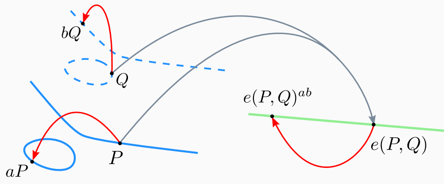
$ e(P+Q, R) = e(P, R) * e(Q, R) $

$ e(aP, Q) = e(P, Q)^a $

So, a scalar $a$ acting in the first operand as $aP$, finds its way out and escapes from the input of the pairing and appears in the output of the pairing as an exponent in $\mathbb{G}_T$. The same linear map is observed for the second group:

$ e(P, Q+R) = e(P, Q) * e(P, R) $

$ e(P, bQ) = e(P, Q)^b $

Hence, the pairing is bilinear. We will see below how this property becomes useful.

Can bilinear pairings help solving ECDLP?

The MOV (by Menezes, Okamoto, and Vanstone) attack reduces the discrete logarithm problem on elliptic curves to finite fields. An attacker with knowledge of $kP$ and public points $P$ and $Q$ can recover $k$ by computing:

$ g_k = e(kP, Q) = e(P, Q)^k $,

$ g = e(P, Q) $

$ k = \log_g(g_k) $

Note that the discrete logarithm to be solved was moved from $\mathbb{G}_1$ to $\mathbb{G}_T$. So an attacker must ensure that the discrete logarithm is easier to solve in $\mathbb{G}_T$, and surprisingly, for some curves this is the case.

Fortunately, pairings do not present a threat for standard curves (such as the NIST curves or Curve25519) because these curves are constructed in such a way that $\mathbb{G}_T$ gets very large, which makes the pairing operation not efficient anymore.

This attacking strategy was one of the first applications of pairings in cryptanalysis as a tool to solve the discrete logarithm. Later, more people noticed that the properties of pairings are so useful, and can be used constructively to do cryptography. One of the fascinating truisms of cryptography is that one person’s sledgehammer is another person’s brick: while pairings yield a generic attack strategy for the ECDLP problem, it can also be used as a building block in a ton of useful applications.

Applications of Pairings

In the 2000s decade, a large wave of research works were developed aimed at applying pairings to many practical problems. An iconic pairing-based system was created by Antoine Joux, who constructed a one-round Diffie-Hellman key exchange for three parties.

Let’s see first how a three-party Diffie-Hellman is done without pairings. Alice, Bob and Charlie want to agree on a shared key, so they compute, respectively, $aP$, $bP$ and $cP$ for a public point P. Then, they send to each other the points they computed. So Alice receives $cP$ from Charlie and sends $aP$ to Bob, who can then send $baP$ to Charlie and get $acP$ from Alice and so on. After all this is done, they can all compute $k=abcP$. Can this be performed in a single round trip?

Pairings in CIRCL
Two round Diffie-Hellman without pairings.
Pairings in CIRCL
One round Diffie-Hellman with pairings.

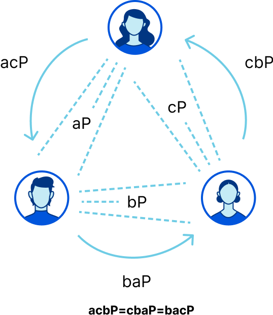
The 3-party Diffie-Hellman protocol needs two communication rounds (on the top), but with the use of pairings a one-round trip protocol is possible.

Affirmative! Antoine Joux showed how to agree on a shared secret in a single round of communication. Alice announces $aP$, gets $bP$ and $cP$ from Bob and Charlie respectively, and then computes $k= (bP, cP)^a$. Likewise Bob computes $e(aP,cP)^b$ and Charlie does $e(aP,bP)^c$. It’s not difficult to convince yourself that all these values are equivalent, just by looking at the bilinear property.

$e(bP,cP)^a  = e(aP,cP)^b  = e(aP,bP)^c = e(P,P)^{abc}$

With pairings we’ve done in one round what would otherwise take two.

Another application in cryptography addresses a problem posed by Shamir in 1984: does there exist an encryption scheme in which the public key is an arbitrary string? Imagine if your public key was your email address. It would be easy to remember and certificate authorities and certificate management would be unnecessary.

A solution to this problem came some years later, in 2001, and is the Identity-based Encryption (IBE) scheme proposed by Boneh and Franklin, which uses bilinear pairings as the main tool.

Nowadays, pairings are used for the zk-SNARKS that make Zcash an anonymous currency, and are also used in drand to generate public-verifiable randomness. Pairings and the compact, aggregatable BLS signatures are used in Ethereum. We have used pairings to build Geo Key Manager: pairings let us implement a compact broadcast and negative broadcast scheme that together make Geo Key Manager work.

In order to make these schemes, we have to implement pairings, and to do that we need to understand the mathematics behind them.

Where do pairings come from?

In order to deeply understand pairings we must understand the interplay of geometry and arithmetic, and the origins of the group’s law. The starting point is the concept of a divisor, a formal combination of points on the curve.

$D = \sum n_i P_i$

The sum of all the coefficients $n_i$ is the degree of the divisor. If we have a function on the curve that has poles and zeros, we can count them with multiplicity to get a principal divisor. Poles are counted as negative, while zeros as positive. For example if we take the projective line, the function $x$ has the divisor $(0)-(\infty)$.

The degree of a divisor is the sum of its coefficients. All principal divisors have degree $0$.  The group of degree zero divisors modulo the principal divisors is the Jacobian. This means that we take all the degree zero divisors, and freely add or subtract principle divisors, constructing an abelian variety called the Jacobian.

Until now our constructions have worked for any curve.  Elliptic curves have a special property: since a line intersects the curve in three points, it’s always possible to turn an element of the Jacobian into one of the form $(P)-(O)$ for a point $P$. This is where the addition law of elliptic curves comes from.

Pairings in CIRCL
The relation between addition on an elliptic curve and the geometry of the curve. Source file ECClines.svg

Given a function $f$ we can evaluate it on a divisor $D=\sum n_i P_i$ by taking the product $\prod f(P_i)^{n_i}$. And if two functions $f$ and $g$ have disjoint divisors, we have the Weil duality:

$ f(\text{div}(g)) = g(\text{div}(f)) $,

The existence of Weil duality is what gives us the bilinear map we seek. Given an $r$-torsion point $T$ we have a function $f$ whose divisor is $r(T)-r(O)$. We can write down an auxiliary function $g$ such that $f(rP)=g^r(P)$ for any $P$. We then get a pairing by taking.

$e_r(S,T)=\frac{g(X+S)}{g(X)}$.

The auxiliary point $X$ is any point that makes the numerator and denominator defined.

In practice, the pairing we have defined above, the Weil pairing, is little used. It was historically the first pairing and is extremely important in the mathematics of elliptic curves, but faster alternatives based on more complicated underlying mathematics are used today. These faster pairings have different $\mathbb{G}_1$ and $\mathbb{G}_2$, while the Weil pairing made them the same.

Shift in parameters

As we saw earlier, the discrete logarithm problem can be attacked either on the group of elliptic curve points or on the third group (an extension of a prime field) whichever is weaker. This is why the parameters that define a pairing must balance the security of the three groups.

Before 2015 a good balance between the extension degree, the size of the prime field, and the security of the scheme was achieved by the family of Barreto-Naehrig (BN) curves. For 128 bits of security, BN curves use an extension of degree 12, and have a prime of size 256 bits; as a result they are an efficient choice for implementation.

A breakthrough for pairings occurred in 2015 when Kim and Barbescu published a result that accelerated the attacks in finite fields. This resulted in increasing the size of fields to comply with standard security levels. Just as short hashes like MD5 got depreciated as they became insecure and $2^{64}$ was no longer enough, and RSA-1024 was replaced with RSA-2048, we regularly change parameters to deal with improved attacks.

For pairings this implied the use of larger primes for all the groups. Roughly speaking, the previous 192-bit security level becomes the new 128-bit level after this attack. Also, this shift in parameters brings the family of Barreto-Lynn-Scott (BLS) curves to the stage because pairings on BLS curves are faster than BN in this new setting. Hence, currently BLS curves using an extension of degree 12, and primes of around 384 bits provide the equivalent to 128 bit security.

The IETF draft (currently in preparation) draft-irtf-cfrg-pairing-friendly-curves specifies secure pairing-friendly elliptic curves. It includes parameters for BN and BLS families of curves. It also targets different security levels to provide crypto agility for some applications relying on pairing-based cryptography.

Implementing Pairings in Go

Historically, notable examples of software libraries implementing pairings include PBC by Ben Lynn, Miracl by Michael Scott, and Relic by Diego Aranha. All of them are written in C/C++ and some ports and wrappers to other languages exist.

In the Go standard library we can find the golang.org/x/crypto/bn256 package by Adam Langley, an implementation of a pairing using a BN curve with 256-bit prime. Our colleague Brendan McMillion built github.com/cloudflare/bn256 that dramatically improves the speed of pairing operations for that curve. See the RWC-2018 talk to see our use case of pairing-based cryptography. This time we want to go one step further, and we started looking for alternative pairing implementations.

Although one can find many libraries that implement pairings, our goal is to rely on one that is efficient, includes protection against side channels, and exposes a flexible API oriented towards applications that permit generality, while avoiding common security pitfalls. This motivated us to include pairings in CIRCL. We followed best practices on secure code development and we want to share with you some details about the implementation.

We started by choosing a pairing-friendly curve. Due to the attack previously mentioned, the BN256 curve does not meet the 128-bit security level. Thus there is a need for using stronger curves. Such a stronger curve is the BLS12-381 curve that is widely used in the zk-SNARK protocols and short signature schemes. Using this curve allows us to make our Go pairing implementation interoperable with other implementations available in other programming languages, so other projects can benefit from using CIRCL too.

This code snippet tests the linearity property of pairings and shows how easy it is to use our library.

import (
    "crypto/rand"
    "fmt"
    e "github.com/cloudflare/circl/ecc/bls12381"
)

func ExamplePairing() {
    P,  Q := e.G1Generator(), e.G2Generator()
    a,  b := new(e.Scalar), new(e.Scalar)
    aP, bQ := new(e.G1), new(e.G2)
    ea, eb := new(e.Gt), new(e.Gt)

    a.Random(rand.Reader)
    b.Random(rand.Reader)

    aP.ScalarMult(a, P)
    bQ.ScalarMult(b, Q)

    g  := e.Pair( P, Q)
    ga := e.Pair(aP, Q)
    gb := e.Pair( P,bQ)

    ea.Exp(g, a)
    eb.Exp(g, b)
    linearLeft := ea.IsEqual(ga) // e(P,Q)^a == e(aP,Q)
    linearRight:= eb.IsEqual(gb) // e(P,Q)^b == e(P,bQ)

    fmt.Print(linearLeft && linearRight)
    // Output: true
}

We applied several optimizations that allowed us to improve on performance and security of the implementation. In fact, as the parameters of the curve are fixed, some other optimizations become easier to apply; for example, the code for prime field arithmetic and the towering construction for extension fields as we detail next.

Formally-verified arithmetic using fiat-crypto

One of the more difficult parts of a cryptography library to implement correctly is the prime field arithmetic. Typically people specialize it for speed, but there are many tedious constraints on what the inputs to operations can be to ensure correctness. Vulnerabilities have happened when people get it wrong, across many libraries. However, this code is perfect for machines to write and check. One such tool is fiat-crypto.

Using fiat-crypto to generate the prime field arithmetic means that we have a formal verification that the code does what we need. The fiat-crypto tool is invoked in this script, and produces Go code for addition, subtraction, multiplication, and squaring over the 381-bit prime field used in the BLS12-381 curve. Other operations are not covered, but those are much easier to check and analyze by hand.

Another advantage is that it avoids relying on the generic big.Int package, which is slow, frequently spills variables to the heap causing dynamic memory allocations, and most importantly, does not run in constant-time. Instead, the code produced is straight-line code, no branches at all, and relies on the math/bits package for accessing machine-level instructions. Automated code generation also means that it’s easier to apply new techniques to all primitives.

Tower Field Arithmetic

In addition to prime field arithmetic, say integers modulo a prime number p, a pairing also requires high-level arithmetic operations over extension fields.

To better understand what an extension field is, think of the analogous case of going from the reals to the complex numbers: the operations are referred as usual, there exist addition, multiplication and division $(+, -, \times, /)$, however they are computed quite differently.

The complex numbers are a quadratic extension over the reals, so imagine a two-level house. The first floor is where the real numbers live, however, they cannot access the second floor by themselves. On the other hand, the complex numbers can access the entire house through the use of a staircase. The equation $f(x)=x^2+1$ was not solvable over the reals, but is solvable over the complex numbers, since they have the number $i^2=1$. And because they have the number $i$, they also have to have numbers like $3i$ and $5+i$ that solve other equations that weren’t solvable over the reals either. This second story has given the roots of the polynomials a place to live.

Algebraically we can view the complex numbers as $\mathbb{R}[x]/(x^2+1)$, the space of polynomials where we consider $x^2=-1$. Given a polynomial like $x^3+5x+1$, we can turn it into $4x+1$, which is another way of writing $1+4i$. In this new field $x^2+1=0$ holds automatically, and we have added both $x$ as a root of the polynomial we picked. This process of writing down a field extension by adding a root of a polynomial works over any field, including finite fields.

Following this analogy, one can construct not a house but a tower, say a $k=12$ floor building where the ground floor is the prime field $\mathbb{F}_p$. The reason to build such a large tower is because we want to host VIP guests: namely a group called $\mu_r$, the $r$-roots of unity. There are exactly $r$ members and they behave as an (algebraic) group, i.e. for all $x,y \in \mu_r$, it follows $x*y \in \mu_r$ and $x^r = 1$.

One particularity is that making operations on the top-floor can be costly. Assume that whenever an operation is needed in the top-floor, members who live on the main floor are required to provide their assistance. Hence an operation on the top-floor needs to go all the way down to the ground floor. For this reason, our tower needs more than a staircase, it needs an efficient way to move between the levels, something even better than an elevator.

What if we use portals? Imagine anyone on the twelfth floor using a portal to go down immediately to the sixth floor, and then use another one connecting the sixth to the second floor, and finally another portal connecting to the ground floor. Thus, one can get faster to the first floor rather than descending through a long staircase.

The building analogy can be used to understand and construct a tower of finite fields. We use only some extensions to build a twelfth extension from the (ground) prime field $\mathbb{F}_p$.

$\mathbb{F}_{p}$ ⇒  $\mathbb{F}_{p^2}$ ⇒  $\mathbb{F}_{p^4}$ ⇒  $\mathbb{F}_{p^{12}}$

In fact, the extension of finite fields is as follows:

  • $\mathbb{F}_{p^2}$ is built as polynomials in $\mathbb{F}_p[u]$ reduced modulo $u^2+1=0$.
  • $\mathbb{F}_{p^6}$ is built as polynomials in $\mathbb{F}_{p^2}[v]$ reduced modulo $v^2+u+1=0$.
  • $\mathbb{F}_{p^{12}}$ is built as polynomials in $\mathbb{F}_{p^6}[w]$ reduced modulo $w^2+v=0$, or as polynomials in $\mathbb{F}_{p^4}[w]$ reduced modulo $w^3+v=0$.

The portals here are the polynomials used as modulus, as they allow us to move from one extension to the other.

Different constructions for higher extensions have an impact on the number of operations performed. Thus, we implemented the latter tower field for $\mathbb{F}_{p^{12}}$ as it results in a lower number of operations. The arithmetic operations are quite easy to implement and manually verify, so at this level formal verification is not as effective as in the case of prime field arithmetic. However, having an automated tool that generates code for this arithmetic would be useful for developers not familiar with the internals of field towering. The fiat-crypto tool keeps track of this idea [Issue 904, Issue 851].

Now, we describe more details about the main core operations of a bilinear pairing.

The Miller loop and the final exponentiation

The pairing function we implemented is the optimal r-ate pairing, which is defined as:

$ e(P,Q) = f_Q(P)^{\text{exp}} $

That is the construction of a function $f$ based on $Q$, then evaluated on a point $P$, and the result of that is raised to a specific power. The efficient function evaluation is performed using “the Miller loop”, which is an algorithm devised by Victor Miller and has a similar structure to a double-and-add algorithm for scalar multiplication.

After having computed $f_Q(P)$ this value is an element of $\mathbb{F}_{p^{12}}$, however it is not yet an $r$-root of unity; in order to do so, the final exponentiation accomplishes this task. Since the exponent is constant for each curve, special algorithms can be tuned for it.

One interesting acceleration opportunity presents itself: in the Miller loop the elements of $\mathbb{F}_{p^{12}}$ that we have to multiply by are special — as polynomials, they have no linear term and their constant term lives in $\mathbb{F}_{p^{2}}$. We created a specialized multiplication that avoids multiplications where the input has to be zero. This specialization accelerated the pairing computation by 12%.

So far, we have described how the internal operations of a pairing are performed. There are still some other functions floating around regarding the use of pairings in cryptographic protocols. It is also important to optimize these functions and now we will discuss some of them.

Product of Pairings

Often protocols will want to evaluate a product of pairings, rather than a single pairing. This is the case if we’re evaluating multiple signatures, or if the protocol uses cancellation between different equations to ensure security, as in the dual system encoding approach to designing protocols. If each pairing was evaluated individually, this would require multiple evaluations of the final exponentiation. However, we can evaluate the product first, and then evaluate the final exponentiation once. This requires a different interface that can take vectors of points.

Occasionally, there is a sign or an exponent in the factors of the product. It’s very easy to deal with a sign explicitly by negating one of the input points, almost for free. General exponents are more complicated, especially when considering the need for side channel protection. But since we expose the interface, later work on the library will accelerate it without changing applications.

Regarding API exposure, one of the trickiest and most error prone aspects of software engineering is input validation. So we must check that raw binary inputs decode correctly as the points used for a pairing. Part of this verification includes subgroup membership testing which is the topic we discuss next.

Subgroup Membership Testing

Checking that a point is on the curve is easy, but checking that it has the right order is not: the classical way to do this is an entire expensive scalar multiplication. But implementing pairings involves the use of many clever tricks that help to make things run faster.

One example is twisting: the $\mathbb{G}_2$ group are points with coordinates in $\mathbb{F}_{p^{12}}$, however, one can use a smaller field to reduce the number of operations. The trick here is using an associated curve $E’$, which is a twist of the original curve $E$. This allows us to work on the subfield $\mathbb{F}_{p^{2}}$ that has cheaper operations.

Additionally, twisting the curve over $\mathbb{G}_2$ carries some efficiently computable endomorphisms coming from the field structure. For the cost of two field multiplications, we can compute an additional endomorphism, dramatically decreasing the cost of scalar multiplication.

By searching for the smallest combination of scalars that could zero out the $r$-torsion points, Sean Bowe came up with a much more efficient way to do subgroup checks. We implement his trick, with a big reduction in the complexity of some applications.

As can be seen, implementing a pairing is full of subtleties. We just saw that point validation in the pairing setting is a bit more challenging than in the conventional case of elliptic curve cryptography. This kind of reformulation also applies to other operations that require special care on their implementation. One another example is how to encode binary strings as elements of the group $\mathbb{G}_1$ (or $\mathbb{G}_2$). Although this operation might sound simple, implementing it securely needs to take into consideration several aspects; thus we expand more on this topic.

Hash to Curve

An important piece on the Boneh-Franklin Identity-based Encryption scheme is a special hash function that maps an arbitrary string — the identity, e.g., an email address — to a point on an elliptic curve, and that still behaves as a conventional cryptographic hash function (such as SHA-256) that is hard to invert and collision-resistant. This operation is commonly known as hashing to curve.

Boneh and Franklin found a particular way to perform hashing to curve: apply a conventional hash function to the input bitstring, and interpret the result as the $y$-coordinate of a point, then from the curve equation $y^2=x^3+b$, find the $x$-coordinate as $x=\sqrt[3]{y^2-b}$. The cubic root always exists on fields of characteristic $p\equiv 2 \bmod{3}$. But this algorithm does not apply to other fields in general restricting the parameters to be used.

Another popular algorithm, but since now we need to remark it is an insecure way for performing hash to curve is the following. Let the hash of the input be the $x$-coordinate, and from it find the $y$-coordinate by computing a square root $y= \sqrt{x^3+b}$. Note that not all $x$-coordinates lead that the square root exists, which means the algorithm may fail; thus, it’s a probabilistic algorithm. To make sure it works always, a counter can be added to $x$ and increased everytime the square root is not found. Although this algorithm always finds a point on the curve, this also makes the algorithm run in variable time i.e., it’s a non-constant time algorithm. The lack of this property on implementations of cryptographic algorithms makes them susceptible to timing attacks. The DragonBlood attack is an example of how a non-constant time hashing algorithm resulted in a full key recovery of WPA3 Wi-Fi passwords.

Secure hash to curve algorithms must guarantee several properties. It must be ensured that any input passed to the hash produces a point on the targeted group. That is no special inputs must trigger exceptional cases, and the output point must belong to the correct group. We make emphasis on the correct group since in certain applications the target group is the entire set of points of an elliptic curve, but in other cases, such as in the pairing setting, the target group is a subgroup of the entire curve, recall that $\mathbb{G}_1$ and $\mathbb{G}_2$ are $r$-torsion points. Finally, some cryptographic protocols are proven secure provided that the hash to curve function behaves as a random oracle of points. This requirement adds another level of complexity to the hash to curve function.

Fortunately, several researchers have addressed most of these problems and some other researchers have been involved in efforts to define a concrete specification for secure algorithms for hashing to curves, by extending the sort of geometric trick that worked for the Boneh-Franklin curve. We have participated in the Crypto Forum Research Group (CFRG) at IETF on the work-in-progress Internet draft-irtf-cfrg-hash-to-curve. This document specifies secure algorithms for hashing targeting several elliptic curves including the BLS12-381 curve. At Cloudflare, we are actively collaborating in several working groups of IETF, see Jonathan Hoyland’s post to know more about it.

Our implementation complies with the recommendations given in the hash to curve draft and also includes many implementation techniques and tricks derived from a vast number of academic research articles in pairing-based cryptography. A good compilation of most of these tricks is delightfully explained by Craig Costello.

We hope this post helps you to shed some light and guidance on the development of pairing-based cryptography, as it has become much more relevant these days. We will share with you soon an interesting use case in which the application of pairing-based cryptography helps us to harden the security of our infrastructure.

What’s next?

We invite you to use our CIRCL library, now equipped with bilinear pairings. But there is more: look at other primitives already available such as HPKE, VOPRF, and Post-Quantum algorithms. On our side, we will continue improving the performance and security of our library, and let us know if any of your projects uses CIRCL, we would like to know your use case. Reach us at research.cloudflare.com.

You’ll soon hear more about how we’re using CIRCL across Cloudflare.

Exported Authenticators: The long road to RFC

Post Syndicated from Jonathan Hoyland original https://blog.cloudflare.com/exported-authenticators-the-long-road-to-rfc/

Exported Authenticators: The long road to RFC

Exported Authenticators: The long road to RFC

Our earlier blog post talked in general terms about how we work with the IETF. In this post we’re going to talk about a particular IETF project we’ve been working on, Exported Authenticators (EAs). Exported Authenticators is a new extension to TLS that we think will prove really exciting. It unlocks all sorts of fancy new authentication possibilities, from TLS connections with multiple certificates attached, to logging in to a website without ever revealing your password.

Now, you might have thought that given the innumerable hours that went into the design of TLS 1.3 that it couldn’t possibly be improved, but it turns out that there are a number of places where the design falls a little short. TLS allows us to establish a secure connection between a client and a server. The TLS connection presents a certificate to the browser, which proves the server is authorised to use the name written on the certificate, for example blog.cloudflare.com. One of the most common things we use that ability for is delivering webpages. In fact, if you’re reading this, your browser has already done this for you. The Cloudflare Blog is delivered over TLS, and by presenting a certificate for blog.cloudflare.com the server proves that it’s allowed to deliver Cloudflare’s blog.

When your browser requests blog.cloudflare.com you receive a big blob of HTML that your browser then starts to render. In the dim and distant past, this might have been the end of the story. Your browser would render the HTML, and display it. Nowadays, the web has become more complex, and the HTML your browser receives often tells it to go and load lots of other resources. For example, when I loaded the Cloudflare blog just now, my browser made 73 subrequests.

As we mentioned in our connection coalescing blog post, sometimes those resources are also served by Cloudflare, but on a different domain. In our connection coalescing experiment, we acquired certificates with a special extension, called a Subject Alternative Name (SAN), that tells the browser that the owner of the certificate can act as two different websites. Along with some further shenanigans that you can read about in our blog post, this lets us serve the resources for both the domains over a single TLS connection.

Cloudflare, however, services millions of domains, and we have millions of certificates. It’s possible to generate certificates that cover lots of domains, and in fact this is what Cloudflare used to do. We used to use so-called “cruise-liner” certificates, with dozens of names on them. But for connection coalescing this quickly becomes impractical, as we would need to know what sub-resources each webpage might request, and acquire certificates to match. We switched away from this model because issues with individual domains could affect other customers.

What we’d like to be able to do is serve as much content as possible down a single connection. When a user requests a resource from a different domain they need to perform a new TLS handshake, costing valuable time and resources. Our connection coalescing experiment showed the benefits when we know in advance what resources are likely to be requested, but most of the time we don’t know what subresources are going to be requested until the requests actually arrive. What we’d rather do is attach extra identities to a connection after it’s been established, and we know what extra domains the client actually wants. Because the TLS connection is just a transport mechanism and doesn’t understand the information being sent across it, it doesn’t actually know what domains might subsequently be requested. This is only available to higher-layer protocols such as HTTP. However, we don’t want any website to be able to impersonate another, so we still need to have strong authentication.

Exported Authenticators

Enter Exported Authenticators. They give us even more than we asked for. They allow us to do application layer authentication that’s just as strong as the authentication you get from TLS, and then tie it to the TLS channel. Now that’s a pretty complicated idea, so let’s break it down.

To understand application layer authentication we first need to explain what the application layer is. The application layer is a reference to the OSI model. The OSI model describes the various layers of abstraction we use, to make things work across the Internet. When you’re developing your latest web application you don’t want to have to worry about how light is flickered down a fibre optic cable, or even how the TLS handshake is encoded (although that’s a fascinating topic in its own right, let’s leave that for another time.)

All you want to care about is having your content delivered to your end-user, and using TLS gives you a guaranteed in-order, reliable, authenticated channel over which you can communicate. You just shove bits in one end of the pipe, and after lots of blinky lights, fancy routing, maybe a touch of congestion control, and a little decoding, *poof*, your data arrives at the end-user.

The application layer is the top of the OSI stack, and contains things like HTTP. Because the TLS handshake is lower in the stack, the application is oblivious to this process. So, what Exported Authenticators give us is the ability for the very top of the stack to reliably authenticate their partner.

Exported Authenticators: The long road to RFC
The seven-layered OSI model

Now let’s jump back a bit, and discuss what we mean when we say that EAs give us authentication that’s as strong as TLS authentication. TLS, as we know, is used to create a secure connection between two endpoints, but lots of us are hazy when we try and pin down exactly what we mean by “secure”. The TLS standard makes eight specific promises, but rather than get buried in that particular ocean of weeds, let’s just pick out the one guarantee that we care about most: Peer Authentication.

Peer authentication: The client's view of the peer identity should reflect the server's identity. [...]

In other words, if the client thinks that it’s talking to example.com then it should, in fact, be talking to example.com.

What we want from EAs is that if I receive an EA then I have cryptographic proof that the person I’m talking to is the person I think I’m talking to. Now at this point you might be wondering what an EA actually looks like, and what it has to do with certificates. Well, an EA is actually a trio of messages, the first of which is a Certificate. The second is a CertificateVerify, a cryptographic proof that the sender knows the private key for the certificate. Finally there is a Finished message, which acts as a MAC, and proves the first two parts of the message haven’t been tampered with. If this structure sounds familiar to you, it’s because it’s the same structure as used by the server in the TLS handshake to prove it is the owner of the certificate.

The final piece of unpacking we need to do is explaining what we mean by tying the authentication to the TLS channel. Because EAs are an application layer construct they don’t provide any transport mechanism. So, whilst I know that the EA was created by the server I want to talk to, without binding the EA to a TLS connection I can’t be sure that I’m talking directly to the server I want.

Exported Authenticators: The long road to RFC
Without protection, a malicious server can move Exported Authenticators from one connection to another.

For all I know, the TLS server I’m talking to is creating a new TLS connection to the EA Server, and relaying my request, and then returning the response. This would be very bad, because it would allow a malicious server to impersonate any server that supports EAs.

Exported Authenticators: The long road to RFC
Because EAs are bound to a single TLS connection, if a malicious server copies an EA from one connection to another it will fail to verify.

EAs therefore have an extra security feature. They use the fact that every TLS connection is guaranteed to produce a unique set of keys. EAs take one of these keys and use it to construct the EA. This means that if some malicious third-party copies an EA from one TLS session to another, the recipient wouldn’t be able to validate it. This technique is called channel binding, and is another fascinating topic, but this post is already getting a bit long, so we’ll have to revisit channel binding in a future blog post.

How the sausage is made

OK, now we know what EAs do, let’s talk about how they were designed and built. EAs are going through the IETF standardisation process. Draft standards move through the IETF process starting as Internet Drafts (I-Ds), and ending up as published Requests For Comment (RFCs). RFCs are voluntary standards that underpin much of the global Internet plumbing, and not just for security protocols like TLS. RFCs define DNS, UDP, TCP, and many, many more.

The first step in producing a new IETF standard is coming up with a proposal. Designing security protocols is a very conservative business, firstly because it’s very easy to introduce really subtle bugs, and secondly, because if you do introduce a security issue, things can go very wrong, very quickly. A flaw in the design of a protocol can be especially problematic as it can be replicated across multiple independent implementations — for example the TLS renegotiation vulnerabilities reported in 2009 and the custom EC(DH) parameters vulnerability from 2012. To minimise the risks of design issues, EAs hew closely to the design of the TLS 1.3 handshake.

Security and Assurance

Before making a big change to how authentication works on the Internet, we want as much assurance as possible that we’re not going to break anything. To give us more confidence that EAs are secure, they reuse parts of the design of TLS 1.3. The TLS 1.3 design was carefully examined by dozens of experts, and underwent multiple rounds of formal analysis — more on that in a moment. Using well understood design patterns is a super important part of security protocols. Making something secure is incredibly difficult, because security issues can be introduced in thousands of ways, and an attacker only needs to find one. By starting from a well understood design we can leverage the years of expertise that went into it.

Another vital step in catching design errors early is baked into the IETF process: achieving rough consensus. Although the ins and outs of the IETF process are worthy of their own blog post, suffice it to say the IETF works to ensure that all technical objections get addressed, and even if they aren’t solved they are given due care and attention. Exported Authenticators were proposed way back in 2016, and after many rounds of comments, feedback, and analysis the TLS Working Group (WG) at the IETF has finally reached consensus on the protocol. All that’s left before the EA I-D becomes an RFC is for a final revision of the text to be submitted and sent to the RFC Editors, leading hopefully to a published standard very soon.

As we just mentioned, the WG has to come to a consensus on the design of the protocol. One thing that can hold up achieving consensus are worries about security. After the Snowden revelations there was a barrage of attacks on TLS 1.2, not to mention some even earlier attacks from academia. Changing how trust works on the Internet can be pretty scary, and the TLS WG didn’t want to be caught flat-footed. Luckily this coincided with the maturation of some tools and techniques we can use to get mathematical guarantees that a protocol is secure. This class of techniques is known as formal methods. To help ensure that people are confident in the security of EAs I performed a formal analysis.

Formal Analysis

Formal analysis is a special technique that can be used to examine security protocols. It creates a mathematical description of the protocol, the security properties we want it to have, and a model attacker. Then, aided by some sophisticated software, we create a proof that the protocol has the properties we want even in the presence of our model attacker. This approach is able to catch incredibly subtle edge cases, which, if not addressed, could lead to attacks, as has happened before. Trotting out a formal analysis gives us strong assurances that we haven’t missed any horrible issues. By sticking as closely as possible to the design of TLS 1.3 we were able to repurpose much of the original analysis for EAs, giving us a big leg up in our ability to prove their security. Our EA model is available in Bitbucket, along with the proofs. You can check it out using Tamarin, a theorem prover for security protocols.

Formal analysis, and formal methods in general, give very strong guarantees that rule out entire classes of attack. However, they are not a panacea. TLS 1.3 was subject to a number of rounds of formal analysis, and yet an attack was still found. However, this attack in many ways confirms our faith in formal methods. The attack was found in a blind spot of the proof, showing that attackers have been pushed to the very edges of the protocol. As our formal analyses get more and more rigorous, attackers will have fewer and fewer places to search for attacks. As formal analysis has become more and more practical, more and more groups at the IETF have been asking to see proofs of security before standardising new protocols. This hopefully will mean that future attacks on protocol design will become rarer and rarer.

Once the EA I-D becomes an RFC, then all sorts of cool stuff gets unlocked — for example OPAQUE-EAs, which will allow us to do password-based login on the web without the server ever seeing the password! Watch this space.

Exported Authenticators: The long road to RFC

Coalescing Connections to Improve Network Privacy and Performance

Post Syndicated from Talha Paracha original https://blog.cloudflare.com/connection-coalescing-experiments/

Coalescing Connections to Improve Network Privacy and Performance

Coalescing Connections to Improve Network Privacy and Performance

Web pages typically have a large number of embedded subresources (e.g., JavaScript, CSS, image files, ads, beacons) that are fetched by a browser on page loads. Requests for these subresources can prompt browsers to perform further DNS lookups, TCP connections, and TLS handshakes, which can have a significant impact on how long it takes for the user to see the content and interact with the page. Further, each additional request exposes metadata (such as plaintext DNS queries, or unencrypted SNI in TLS handshake) which can have potential privacy implications for the user. With these factors in mind, we carried out a measurement study to understand how we can leverage Connection Coalescing (aka Connection Reuse) to address such concerns, and study its feasibility.

Background

The web has come a long way and initially consisted of very simple protocols. One of them was HTTP/1.0, which required browsers to make a separate connection for every subresource on the page. This design was quickly recognized as having significant performance bottlenecks and was extended with HTTP pipelining and persistent connections in HTTP/1.1 revision, which allowed HTTP requests to reuse the same TCP connection. But, yet again, this was no silver bullet: while multiple requests could share the same connection, they still had to be serialized one after the other, so a client and server could only execute a single request/response exchange at any given time for each connection. As time passed, websites became more complex in structure and dynamic in nature, and HTTP/1.1 was identified as a major bottleneck. The only way to gain concurrency at the network layer was to use multiple TCP connections to the same origin in parallel, but this meant losing most benefits of persistent connections and ended up overloading the origin servers which were unable to meet the concurrency demand.

To address these performance limitations, the SPDY protocol was introduced over a decade later. SPDY supported stream multiplexing, where requests to and responses from the server used a single interleaved TCP connection, and allowed browsers to prioritize requests for critical subresources first — that were blocking page rendering. A modified variant of SPDY was standardized by the IETF as HTTP/2 in 2012 and published as RFC 7540 in 2015.

HTTP/2 and onwards retained this new standard for connection reuse. More specifically, all subresources on the same domain were able to reuse the same TCP/TLS (or UDP/QUIC) connection without any head-of-line blocking (at least on the application layer). This resulted in a single connection for all the subresources — reducing extraneous requests on page loads — potentially speeding up some websites and applications.

Interestingly, the protocol has a lesser-known feature to also enable subresources at different hostnames to be fetched over the same connection. We studied the real-world feasibility and benefits of this technique as an effort to improve users’ experience for websites across our network.

Coalescing Connections to Improve Network Privacy and Performance
Connection Coalescing allows reusing a TLS connection across different domains

Connection Coalescing

The technique is often referred to as Connection Coalescing and, to put it simply, is a way to access resources from different hostnames that are accessible from the same web server.

There are several reasons for why a single server could handle requests for different hosts, ranging from low-cost virtual hosting to the usage of CDNs and cloud providers (including Cloudflare, that acts as a reverse proxy for approximately 25 million Internet properties). Before going into the technical conditions required to enable connection coalescing, we should take a look at some benefits such a strategy can provide.

  • Privacy. When resources at different hostnames are loaded via separate TLS connections, those connections expose metadata to ISPs and other observers via the Server Name Indicator (SNI) field about the destinations that are being contacted (i.e., in the absence of encrypted SNI). This set of exposed SNI’s can allow an on-path adversary to fingerprint traffic and possibly determine user interactions on the webpage. On the other hand, coalesced requests for more than one hostname on a single connection exposes only one destination, and helps avoid such threats.
  • Performance. Additional TLS handshakes and TCP connections can incur significant costs in terms of cpu, memory and other resources. Thus, coalescing requests to use the same connection can optimize resource utilization.
  • Resource Prioritization. Multiplexing requests on a single connection means that applications have better visibility and more direct control over how related resources are prioritized and scheduled. In the absence of coalescing, the network properties (for example, route congestion) can interfere with the intended order of delivery for resources. This reliability gained through connection coalescing opens up new optimization opportunities to improve web page load times, among other things.

However, along with all these potential benefits, connection coalescing also has some associated risk factors that need to be considered in practice. First, TCP incorporates “fair” congestion control mechanisms — if there are ten connections on the same route, each gets approximately 1/10th of the total bandwidth. So with a route congested and bandwidth restricted, a client relying on multiple connections might be better off (for example, if they have five of the ten connections, their total share of bandwidth would be half). Second, browsers will use different parallelization routines for scheduling requests on multiple connections versus the same connection — it is not immediately clear whether the former or latter would perform better. Third, multiple connections exhibit an inherent form of load balancing for TLS-termination processes. That’s because multiple requests on the same connection must be answered by the same TLS-termination process that holds the session keys (often on the same physical server). So, it is important to study connection coalescing carefully before rolling it out widely.

With this context in mind, we studied the feasibility of connection coalescing on real-world traffic. More specifically, the two questions we wanted to answer were
(a) can we empirically demonstrate and quantify the theoretical benefits of connection coalescing?, and (b) could coalescing cause unintended side effects, such as performance degradation, due to the risks highlighted above?

In order to answer these questions, we first made the observation that a large number of Cloudflare customers request subresources from cdnjs — which is also powered by Cloudflare. For context, cdnjs has public JavaScript and CSS libraries (like jQuery), and is used by more than 12% of all websites on the Internet. One popular way these websites include resources from cdnjs is by using <script src="https://cdnjs.cloudflare.com/..." ></script> HTML tags. But there are other ways as well, such as the usage of XMLHttpRequest or Fetch APIs. Regardless of the way these resources are included, browsers will need to fetch them for completely loading a website.

We then identified a list of approximately four thousand websites using Cloudflare (on the Free plan) that likely used cdnjs. We divided this list of sites into evenly-sized and randomly-picked control and experiment groups. Our plan was to enable coalescing only for the experiment group, so that subresource requests generated from their web pages for cdnjs could reuse existing connections. In this way, we were able to compare results obtained on the experiment group, with the ones for the control group, and attribute any differences observed to connection coalescing.

In order to signal browsers that the requests can be coalesced, we served cdnjs and the sites from the same IP address in a few regions around the world. This meant the same DNS responses for all the zones that were part of the study — eventually load balanced by our Anycast network. These sites also had TLS certificates that included cdnjs.

The above two conditions (same IP and compatible certificate) are required to achieve coalescing as per the HTTP/2 spec. However, the QUIC spec allows coalescing even if only the second condition is met. Major web browsers are yet to adopt the QUIC coalescing mechanism, and currently use only the HTTP/2 coalescing logic for both protocols.

Coalescing Connections to Improve Network Privacy and Performance
Requests to Experiment Group Zones and cdnjs being coalesced on the same TLS connection

Results

We started noticing evidence of real-world coalescing from the day our experiment was launched. The following graph shows that approximately 50% of requests to cdnjs from our experiment group sites are coalesced (i.e., their TLS SNI does not equal cdnjs) as compared to 0% of requests from the control group sites.

Coalescing Connections to Improve Network Privacy and Performance
Coalesced Requests to cdnjs from Control and Experimental Group Zones

In addition, we conducted active measurements using our private WebPageTest instances at the landing pages of experiment and control sites — using the two well-supported browsers: Google Chrome and Firefox. From our results, Chrome created about 78% fewer TLS connections to cdnjs for our experiment group sites, as compared to the control group. But surprisingly, Firefox created just roughly 22% fewer connections. As TLS handshakes are computationally expensive because they involve cryptographic signatures and key exchange algorithms, fewer handshakes meant less CPU cycles spent by both the client and the server.

Upon further analysis, we were able to make two observations from the data:

  • A fraction of sites that never coalesced connections with either browser appeared to load subresources with CORS enabled (i.e., <script src="https://cdnjs.cloudflare.com/..." integrity="sha512-894Y..." crossorigin="anonymous">). This is the default way cdnjs recommends inclusion of subresources, as CORS is needed for integrity checks that provide substantial mitigations against script-manipulation attacks. We do not recommend removing this attribute. Our testing also revealed that using XMLHttpRequest or Fetch APIs to load subresources disabled coalescing as well. It is unclear why browsers choose to not coalesce such connections, and we are in contact with the vendors to find out.
  • Although both Firefox and Chrome coalesced requests for cdnjs on existing connections, the reason for the discrepancy in the number of TLS connections to cdnjs (approximately 78% vs roughly 22%) is because Firefox appears to open new connections even if it does not end up using them.

After evaluating the potential benefits of coalescing, we wanted to understand if coalescing caused any unintended side effects. Hence, the final measurement we conducted was to check whether our experiments were detrimental to a website’s performance. We tracked Page Load Times (PLT) and Largest Contentful Paint (LCP) across a variety of stimulated network conditions using both Chrome and Firefox and found the results for experiment vs control group to not be statistically significant.

Coalescing Connections to Improve Network Privacy and Performance
Page load times for control and experiment group sites. Each site was loaded once, and the “fullyLoaded” metric from WebPageTest is reported

Conclusion

We consider our experimentation successful in determining the feasibility of connection coalescing and highlighting its potential benefits in terms of privacy and performance. More specifically, we observed the privacy benefits of coalescing in more than 50% of requests to cdnjs from real-world traffic. In addition, our active testing demonstrated that browsers create fewer TLS connections with coalescing enabled. Interestingly, our results also revealed that the benefits might not always occur (i.e., CORS-enabled requests, Firefox creating additional TLS connections despite coalescing). Finally, we did not find any evidence that coalescing can cause harm to real-world users’ experience on the Internet.

Some future directions we would like to explore include:

  • More aggressive connection reuse with multiple hostnames, while identifying conditions most suitable for coalescing.
  • Understanding how different connection reuse methods compare, e.g., IP-based coalescing vs. use of Origin Frames, and what effects do they have on user experience over the Internet.
  • Evaluating coalescing support among different browser vendors, and encouraging adoption of HTTP/3 QUIC based coalescing.
  • Reaping the full benefits of connection coalescing by experimenting with custom priority schemes for requests within the same connection.

Please send questions and feedback to [email protected]. We’re excited to continue this line of work in our effort to help build a better Internet! For those interested in joining our team please visit our Careers Page.

Inspiring learners about computing through health and well-being projects | Hello World #17

Post Syndicated from Gemma Coleman original https://www.raspberrypi.org/blog/inspiring-learners-computing-health-well-being-projects-hello-world-17/

Your brand-new issue of the free Hello World magazine for computing educators focuses on all things health and well-being, featuring useful tools for educators, great ideas for schools, and inspiring projects, ideas, and resources from teachers around the world!

Cover of issue 17 of Hello World.

One such project was created by the students of James Abela, Head of Computing at Garden International School in Kuala Lumpur, Raspberry Pi Certified Educator, founder of the South East Asian Computer Science Teachers Association, and author of The Gamified Classroom:

Protecting children from breathing hazardous air

In 2018, Indonesia burned approximately 529,000 hectares of land. That’s an area more than three times the size of Greater London, or almost the size of Brunei. With so much forest being burned, the whole region felt the effects of the pollution. Schools frequently had to ban outdoor play and PE lessons, and on some days schools were closed completely. Many schools in the region had an on-site CO2 detector to know when pollution was bad, but by the time the message could get out, children had already been breathing in the polluted air for several minutes.

A forest fire.
The air pollution from a forest fire gets dispersed by winds and can spread way beyond the area of the fire.

My Year 12 students (aged 16–17) followed the news and weather forecasts intently, and we all started to see how the winds from Singapore and Sumatra were sending pollution to us in Kuala Lumpur. We also realised that if we had measurements from around the city, we might have some visibility as to when pollution was likely to affect our school.

Making room for student-led projects

I’ve always encouraged my students to do their own projects, because it gives programming tasks meaning and creates something that they can be genuinely proud of. The other benefit is that it is something to talk about in university essays and interviews, especially as they often need to do extensive research to solve the problems central to their projects.

This project was […] a genuine passion project in every sense of the word.

James Abela

This project was much more than this: it was a genuine passion project in every sense of the word. Three of my students approached me with the idea of tracking CO2 to give schools a better idea of when there was pollution and which way it was going. They had had some experience of using Raspberry Pi computers, and knew that it was possible to use them to make weather stations, and that the latest versions had wireless LAN capability that they could use. I agreed to support them during allocated programming time, and to help them reach out to other schools.

Circuit design of the CO2 sensor using just Raspberry Pi, designed on circuito.io

I was able to offer students support with this project because I flip quite a lot of the theory in my class. Flipped learning is a teaching approach in which some direct instruction, for example reading articles or watching specific videos, is done at home. This enables more class time to be used to answer questions, work through higher-order tasks, or do group work, and it creates more supervised coding time.

I was able to offer students support with this project because I flip quite a lot of the theory in my class.

James Abela

I initially started doing this because when I set coding challenges for homework, I often had students who confessed they spent all night trying to solve it, only for me to glance at the code and notice a missing colon or indentation issue. I began flipping the less difficult theory for students to do as homework, to create more programming time in class where we could resolve issues more quickly. This then evolved into a system where students could work much more at their own pace and eventually led to a point at which older students could, in effect, learn through their own projects, such as the pollution monitor.

Building the pollution monitor

The students started by looking at existing weather station projects — for example, there is an excellent tutorial on the Raspberry Pi Foundation’s projects site. Students discovered that wind data is relatively easy to get over a larger area, but the key component would be something to measure CO2. […]

Check out issue 17 of Hello World to read the rest of James’s article and find out all the details about the hardware and software his students used for this passion project. He says:

This project really helped these students to decide whether they enjoyed the hardware side of computing, and solving real-world issues really encouraged them to see computing as a practical subject. This is a message that has really resonated with other students, and we’ve since doubled the number of students taking A level computer science.

James Abela

Download the new Hello World for free!

Issue 17 of Hello World is bursting with inspiring ideas for teaching your learners about computing in the context of health and well-being. And you’ll find lots more great content in its 100 pages!

James’s article is also a wonderful example of an educator empowering their students to build a tech project they care about. You’ll discover more insights and practical tips on making computing relevant to all your learners in the following articles of the new Hello World issue:

  • Inspiring Young People With Contexts They Care About
  • Computing for all: Designing a Culturally Relevant Curriculum
  • Going Back to Basics: Part 2 — a follow-on from issue 16 about how to take beginner digital makers through their first physical computing projects

Download the new issue of Hello World for free today:

If you’re an educator based in the UK, you can subscribe to receive each new issue in print completely free! And wherever you are in the world, don’t forget to listen to the Hello World podcast, where each episode we dive into a new topic from the magazine with some of the computing educators who’ve written for us.

The post Inspiring learners about computing through health and well-being projects | Hello World #17 appeared first on Raspberry Pi.

Patch Tuesday – October 2021

Post Syndicated from Greg Wiseman original https://blog.rapid7.com/2021/10/12/patch-tuesday-october-2021/

Patch Tuesday - October 2021

Today’s Patch Tuesday sees Microsoft issuing fixes for over 70 CVEs, affecting the usual mix of their product lines. From Windows, Edge, and Office, to Exchange, SharePoint, and Dynamics, there is plenty of patching to do for workstation and server administrators alike.

One vulnerability has already been seen exploited in the wild: CVE-2021-40449 is an elevation of privilege vulnerability in all supported versions of Windows, including the newly released Windows 11. Rated as Important, this is likely being used alongside Remote Code Execution (RCE) and/or social engineering attacks to gain more complete control of targeted systems.

Three CVEs were publicly disclosed before today, though haven’t yet been observed in active exploitation. CVE-2021-40469 is an RCE vulnerability affecting Microsoft DNS servers, CVE-2021-41335 is another privilege escalation vulnerability in the Windows Kernel, and CVE-2021-41338 is a flaw in Windows AppContainer allowing attackers to bypass firewall rules.

Attackers will likely be paying attention to the latest Windows Print Spooler vulnerability – CVE-2021-36970 is a Spoofing vulnerability with a CVSSv3 score of 8.8 that we don’t yet have much more information about. Also worth noting is CVE-2021-40486, an RCE affecting Microsoft Word, OWA, as well as SharePoint Server, which can be exploited via the Preview Pane. CVE-2021-40487 is another RCE affecting SharePoint Server that Microsoft expects to be exploited before too long.

Another notable vulnerability is CVE-2021-26427, the latest in Exchange Server RCEs. The severity is mitigated by the fact that attacks are limited to a “logically adjacent topology,” meaning that it cannot be exploited directly over the public Internet. Three other vulnerabilities related to Exchange Server were also patched: CVE-2021-41350, a Spoofing vulnerability; CVE-2021-41348, allowing elevation of privilege; and CVE-2021-34453, which is a Denial of Service vulnerability.

Finally, virtualization administrators should be aware of two RCEs affecting Windows Hyper-V: CVE-2021-40461 and CVE-2021-38672. Both affect relatively new versions of Windows and are considered Critical, allowing a VM to escape from guest to host by triggering a memory allocation error, allowing it to read kernel memory in the host.

Summary Charts

Patch Tuesday - October 2021

Summary Tables

Apps Vulnerabilities

CVE Title Exploited Publicly Disclosed? CVSSv3 Base Score has FAQ?
CVE-2021-41363 Intune Management Extension Security Feature Bypass Vulnerability No No 4.2 Yes

Browser Vulnerabilities

CVE Title Exploited Publicly Disclosed? CVSSv3 Base Score has FAQ?
CVE-2021-37980 Chromium: CVE-2021-37980 Inappropriate implementation in Sandbox No No N/A Yes
CVE-2021-37979 Chromium: CVE-2021-37979 Heap buffer overflow in WebRTC No No N/A Yes
CVE-2021-37978 Chromium: CVE-2021-37978 Heap buffer overflow in Blink No No N/A Yes
CVE-2021-37977 Chromium: CVE-2021-37977 Use after free in Garbage Collection No No N/A Yes
CVE-2021-37976 Chromium: CVE-2021-37976 Information leak in core No No N/A Yes
CVE-2021-37975 Chromium: CVE-2021-37975 Use after free in V8 No No N/A Yes
CVE-2021-37974 Chromium: CVE-2021-37974 Use after free in Safe Browsing No No N/A Yes

Developer Tools Vulnerabilities

CVE Title Exploited Publicly Disclosed? CVSSv3 Base Score has FAQ?
CVE-2021-3450 OpenSSL: CVE-2021-3450 CA certificate check bypass with X509_V_FLAG_X509_STRICT No No N/A Yes
CVE-2021-3449 OpenSSL: CVE-2021-3449 NULL pointer deref in signature_algorithms processing No No N/A Yes
CVE-2020-1971 OpenSSL: CVE-2020-1971 EDIPARTYNAME NULL pointer de-reference No No N/A Yes
CVE-2021-41355 .NET Core and Visual Studio Information Disclosure Vulnerability No No 5.7 Yes

ESU Windows Vulnerabilities

CVE Title Exploited Publicly Disclosed? CVSSv3 Base Score has FAQ?
CVE-2021-38663 Windows exFAT File System Information Disclosure Vulnerability No No 5.5 Yes
CVE-2021-40465 Windows Text Shaping Remote Code Execution Vulnerability No No 7.8 No
CVE-2021-36953 Windows TCP/IP Denial of Service Vulnerability No No 7.5 No
CVE-2021-40460 Windows Remote Procedure Call Runtime Security Feature Bypass Vulnerability No No 6.5 Yes
CVE-2021-36970 Windows Print Spooler Spoofing Vulnerability No No 8.8 No
CVE-2021-41332 Windows Print Spooler Information Disclosure Vulnerability No No 6.5 Yes
CVE-2021-41331 Windows Media Audio Decoder Remote Code Execution Vulnerability No No 7.8 No
CVE-2021-41342 Windows MSHTML Platform Remote Code Execution Vulnerability No No 6.8 Yes
CVE-2021-41335 Windows Kernel Elevation of Privilege Vulnerability No Yes 7.8 No
CVE-2021-40455 Windows Installer Spoofing Vulnerability No No 5.5 No
CVE-2021-26442 Windows HTTP.sys Elevation of Privilege Vulnerability No No 7 No
CVE-2021-41340 Windows Graphics Component Remote Code Execution Vulnerability No No 7.8 Yes
CVE-2021-38662 Windows Fast FAT File System Driver Information Disclosure Vulnerability No No 5.5 Yes
CVE-2021-41343 Windows Fast FAT File System Driver Information Disclosure Vulnerability No No 5.5 Yes
CVE-2021-40469 Windows DNS Server Remote Code Execution Vulnerability No Yes 7.2 Yes
CVE-2021-40443 Windows Common Log File System Driver Elevation of Privilege Vulnerability No No 7.8 No
CVE-2021-40466 Windows Common Log File System Driver Elevation of Privilege Vulnerability No No 7.8 No
CVE-2021-40467 Windows Common Log File System Driver Elevation of Privilege Vulnerability No No 7.8 No
CVE-2021-40449 Win32k Elevation of Privilege Vulnerability Yes No 7.8 No
CVE-2021-40489 Storage Spaces Controller Elevation of Privilege Vulnerability No No 7.8 Yes

Exchange Server Vulnerabilities

CVE Title Exploited Publicly Disclosed? CVSSv3 Base Score has FAQ?
CVE-2021-41350 Microsoft Exchange Server Spoofing Vulnerability No No 6.5 No
CVE-2021-26427 Microsoft Exchange Server Remote Code Execution Vulnerability No No 9 Yes
CVE-2021-41348 Microsoft Exchange Server Elevation of Privilege Vulnerability No No 8 No
CVE-2021-34453 Microsoft Exchange Server Denial of Service Vulnerability No No 7.5 No

Microsoft Dynamics Vulnerabilities

CVE Title Exploited Publicly Disclosed? CVSSv3 Base Score has FAQ?
CVE-2021-40457 Microsoft Dynamics 365 Customer Engagement Cross-Site Scripting Vulnerability No No 7.4 Yes
CVE-2021-41353 Microsoft Dynamics 365 (on-premises) Spoofing Vulnerability No No 5.4 No
CVE-2021-41354 Microsoft Dynamics 365 (on-premises) Cross-site Scripting Vulnerability No No 4.1 No

Microsoft Office Vulnerabilities

CVE Title Exploited Publicly Disclosed? CVSSv3 Base Score has FAQ?
CVE-2021-40486 Microsoft Word Remote Code Execution Vulnerability No No 7.8 Yes
CVE-2021-40484 Microsoft SharePoint Server Spoofing Vulnerability No No 7.6 No
CVE-2021-40483 Microsoft SharePoint Server Spoofing Vulnerability No No 7.6 No
CVE-2021-41344 Microsoft SharePoint Server Remote Code Execution Vulnerability No No 8.1 No
CVE-2021-40487 Microsoft SharePoint Server Remote Code Execution Vulnerability No No 8.1 Yes
CVE-2021-40482 Microsoft SharePoint Server Information Disclosure Vulnerability No No 5.3 Yes
CVE-2021-40480 Microsoft Office Visio Remote Code Execution Vulnerability No No 7.8 Yes
CVE-2021-40481 Microsoft Office Visio Remote Code Execution Vulnerability No No 7.1 Yes
CVE-2021-40471 Microsoft Excel Remote Code Execution Vulnerability No No 7.8 Yes
CVE-2021-40473 Microsoft Excel Remote Code Execution Vulnerability No No 7.8 Yes
CVE-2021-40474 Microsoft Excel Remote Code Execution Vulnerability No No 7.8 Yes
CVE-2021-40479 Microsoft Excel Remote Code Execution Vulnerability No No 7.8 Yes
CVE-2021-40485 Microsoft Excel Remote Code Execution Vulnerability No No 7.8 Yes
CVE-2021-40472 Microsoft Excel Information Disclosure Vulnerability No No 5.5 Yes

Microsoft Office Windows Vulnerabilities

CVE Title Exploited Publicly Disclosed? CVSSv3 Base Score has FAQ?
CVE-2021-40454 Rich Text Edit Control Information Disclosure Vulnerability No No 5.5 Yes

System Center Vulnerabilities

CVE Title Exploited Publicly Disclosed? CVSSv3 Base Score has FAQ?
CVE-2021-41352 SCOM Information Disclosure Vulnerability No No 7.5 Yes

Windows Vulnerabilities

CVE Title Exploited Publicly Disclosed? CVSSv3 Base Score has FAQ?
CVE-2021-40464 Windows Nearby Sharing Elevation of Privilege Vulnerability No No 8 No
CVE-2021-40463 Windows NAT Denial of Service Vulnerability No No 7.7 No
CVE-2021-40462 Windows Media Foundation Dolby Digital Atmos Decoders Remote Code Execution Vulnerability No No 7.8 No
CVE-2021-41336 Windows Kernel Information Disclosure Vulnerability No No 5.5 Yes
CVE-2021-38672 Windows Hyper-V Remote Code Execution Vulnerability No No 8 Yes
CVE-2021-40461 Windows Hyper-V Remote Code Execution Vulnerability No No 8 No
CVE-2021-40477 Windows Event Tracing Elevation of Privilege Vulnerability No No 7.8 No
CVE-2021-41334 Windows Desktop Bridge Elevation of Privilege Vulnerability No No 7 No
CVE-2021-40475 Windows Cloud Files Mini Filter Driver Information Disclosure Vulnerability No No 5.5 Yes
CVE-2021-40468 Windows Bind Filter Driver Information Disclosure Vulnerability No No 5.5 Yes
CVE-2021-41347 Windows AppX Deployment Service Elevation of Privilege Vulnerability No No 7.8 No
CVE-2021-41338 Windows AppContainer Firewall Rules Security Feature Bypass Vulnerability No Yes 5.5 No
CVE-2021-40476 Windows AppContainer Elevation Of Privilege Vulnerability No No 7.5 No
CVE-2021-40456 Windows AD FS Security Feature Bypass Vulnerability No No 5.3 Yes
CVE-2021-40450 Win32k Elevation of Privilege Vulnerability No No 7.8 No
CVE-2021-41357 Win32k Elevation of Privilege Vulnerability No No 7.8 No
CVE-2021-40478 Storage Spaces Controller Elevation of Privilege Vulnerability No No 7.8 No
CVE-2021-40488 Storage Spaces Controller Elevation of Privilege Vulnerability No No 7.8 No
CVE-2021-26441 Storage Spaces Controller Elevation of Privilege Vulnerability No No 7.8 Yes
CVE-2021-41345 Storage Spaces Controller Elevation of Privilege Vulnerability No No 7.8 No
CVE-2021-41330 Microsoft Windows Media Foundation Remote Code Execution Vulnerability No No 7.8 No
CVE-2021-41339 Microsoft DWM Core Library Elevation of Privilege Vulnerability No No 4.7 No
CVE-2021-40470 DirectX Graphics Kernel Elevation of Privilege Vulnerability No No 7.8 No
CVE-2021-41346 Console Window Host Security Feature Bypass Vulnerability No No 5.3 No
CVE-2021-41337 Active Directory Security Feature Bypass Vulnerability No No 4.9 Yes
CVE-2021-41361 Active Directory Federation Server Spoofing Vulnerability No No 5.4 Yes

[$] A QEMU case study in grappling with software complexity

Post Syndicated from original https://lwn.net/Articles/872321/rss

There are many barriers to producing software that is reliable and
maintainable over the long term. One of those is software complexity. At
the recently concluded 2021 KVM
Forum
, Paolo Bonzini
explored
this topic, using QEMU, the open source emulator
and virtualizer, as a case study. Drawing on his experience as
a maintainer of several QEMU subsystems, he made some concrete
suggestions on how to defend against undesirable complexity. Bonzini
used QEMU as a running example throughout the talk, hoping to make it
easier for future contributors to modify QEMU. However, the
lessons he shared are equally applicable to many other projects.

Continuous monitoring with Sumo Logic using Amazon Kinesis Data Firehose HTTP endpoints

Post Syndicated from Dilip Rajan original https://aws.amazon.com/blogs/big-data/continuous-monitoring-with-sumo-logic-using-amazon-kinesis-data-firehose-http-endpoints/

Amazon Kinesis Data Firehose streams data to AWS destinations such as Amazon Simple Storage Service (Amazon S3), Amazon Redshift, and Amazon OpenSearch Service (successor to Amazon Elasticsearch Service). Additionally, Kinesis Data Firehose supports destinations to third-party partners. This ability to send data to third-party partners is a vital feature for customers who already use these AWS partner platforms; especially partners specializing in continuous monitoring and intelligence. Kinesis Data Firehose includes sending logs and metrics to Sumo Logic—a cloud machine data analytics and AWS Advanced Technology partner with competencies in containers, data and analytics, DevOps, and security. Sumo Logic helps organizations get better real-time visibility into their IT infrastructure as a result of integrations across cloud and on-premises services, making it simple to aggregate data and giving a full view of your operational, business, and security analytics.

In this post, we go over the Kinesis Data Firehose and Sumo Logic integration and how you can use this feature to stream logs and metrics from Amazon CloudWatch and other AWS services to Sumo Logic. We also go over the key mechanism employed by Sumo Logic to consume logs and its benefits with CloudWatch and AWS Lambda with an example use case.

With this integration, AWS services via CloudWatch metrics have a dedicated and reliable delivery mechanism to Sumo Logic via Kinesis Data Firehose, along with automatic retry capabilities and performant and less intrusive log collection. Let’s look at these benefits in detail:

  • Reliable delivery – This streaming solution doesn’t consume your AWS quota by making calls to the CloudWatch APIs. This rules out the possibility of potential data loss due to API throttling events.
  • Automatic retry capabilities – Kinesis Data Firehose has an automatic retry mechanism and routes all failed logs and metrics to a customer-owned S3 bucket for later recovery.
  • Performant and less intrusive log collection – The solution eliminates the need for creating separate log forwarders such as Lambda functions, which require Sumo Logic to run proprietary code in customer AWS accounts that are limited by timeout, concurrency, and memory limits.
  • Cost benefits – This integration also addresses the additional overhead that comes with the lack of a managed and low code ingestion pipeline, manual management of API quotas, and other ingestion mechanisms such as polling that leads to additional cost.

Solution overview

To illustrate this integration, a sample Lambda function vends metrics and logs to CloudWatch, and are consumed by Sumo Logic through this integration. The following diagram illustrates consumption of CloudWatch logs and metrics for a Lambda function through a Kinesis Data Firehose HTTP endpoint for Sumo Logic.

In the subsequent sections, we show you the Sumo Logic hosted collector and Kinesis Data Firehose setup processes that convert the architecture into meaningful insights.

Prerequisites

Make sure that you have a Lambda function with logs and metrics forwarded to CloudWatch. To get started, use the sample Hello World application.

Configure CloudWatch logs and metrics to be forwarded to Kinesis Data Firehose. You can use the latest CloudWatch features such as subscription filters here as well.

Also sign up for a trial version of Sumo Logic, if you don’t have an account already.

Set up the integration on Sumo Logic

Complete the following instructions to set up a hosted collector on Sumo Logic for Kinesis Data Firehose metrics or logs:

  1. After logging in to Sumo logic, choose Manage Data.
  2. On the Collection menu, and choose Add source.
  3. For the collector selection source, choose Collector-Name.
  4. Choose AWS Kinesis Firehose for Logs or AWS Kinesis Firehose for Metrics.
  5. Provide a collector name and source category required for querying later.
    1. You also need a cross-account role (Sumo Logic provides an AWS CloudFormation template to create the role).
  6. Save your settings.

After you save, an HTTP source address is generated.

  1. Save this endpoint for use with Kinesis Data Firehose.

Sumo Logic provides different endpoints for logs and metrics, for example:

  • Logshttps://endpoint4.collection.us2.sumologic.com/receiver/v1/kinesis/log/<tokenid>
  • Metricshttps://endpoint4.collection.us2.sumologic.com/receiver/v1/kinesis/metric/<tokenid>

Note down the endpoints to use in the following section.

Set up Kinesis Data Firehose

To create a delivery stream on Kinesis Data Firehose, complete the following steps:

  1. On the Kinesis Data Firehose console, choose Create delivery stream.
  2. For Delivery stream name, enter a name.
  3. For Source, select Direct PUT of other sources.
  4. For Destination, choose Sumo Logic.
  5. For HTTP endpoint URL, enter the endpoint URL of the source from Sumo Logic (logs or metrics) that you noted earlier.
  6. In the Backup settings section, select Failed data only.
  7. Keep the rest of the settings at their default values and choose Next.
  8. For Sumo logic Buffer conditions, enter a buffer size of 5 MiB for logs or 1 MiB for metrics.

Configuring the preceding values by type (logs or metrics) is required to achieve optimum latency.

  1. Leave the rest of the settings at their default values and chose Next.
  2. Review your settings and choose Create delivery stream.

Logs and metrics to your delivery stream are now available in Sumo Logic. The following screenshot illustrates a Sumo Logic dashboard for Lambda, which comes out of the box and can be used for observability, analysis, and alerting.

Conclusion

With Kinesis Data Firehose HTTP endpoint delivery, AWS service logs and metrics are available for analysis quickly, so you can identify issues and challenges within your applications. Sumo Logic allows you to gain intelligence across your entire application lifecycle and stack along with analytics and insights to build, operate, and secure your modern applications and cloud infrastructure. As a fully managed service, Kinesis Data Firehose coupled with Sumo Logic compression techniques provides seamless access to logs and metrics.


About the Author

Dilip Rajan is a Partner Solutions Architect at AWS. His role is to help partners and customers design and build solutions at scale on AWS. Before AWS, he helped Amazon Fulfillment Operations migrate their Oracle Data Warehouse to Redshift while designing the next generation big data analytics platform using AWS technologies.

Vinay Maddi is a Senior Solutions Architect for AWS, and passionate about helping customers build modern event driven applications using latest AWS services. An experienced developer, he loves keeping up to date with the latest open-source projects. His main topics are serverless, IoT, AI/ML and blockchain.

This Was the Summer of AppSec: All the Improvements We Made in Q3

Post Syndicated from Tom Caiazza original https://blog.rapid7.com/2021/10/12/this-was-the-summer-of-appsec-all-the-improvements-we-made-in-q3/

This Was the Summer of AppSec: All the Improvements We Made in Q3

Summer has come to an end. The backyard barbecues are behind us, the hot dogs have all been eaten, and we’re all gearing up for some awesome autumn leaf peeping. But before we fall into another season (see what we did there?), we wanted to take a moment to look back on all of the improvements we’ve made to InsightAppSec and tCell over the last 3 months.

At Rapid7, we’re obsessed with making your lives easier, so it’s no surprise that most of our biggest improvements to the platform help our customers do more in less time and with less stress. We took a look at authentication, validation, remediation, and auditing. We’ve punched up our tCell API capabilities, and we’ve rolled these out this summer to give you more time to focus on the important work of securing your applications (and hopefully having a few well-deserved drinks with those little umbrellas in them). In short, we worked hard all summer so that you can sleep easier this fall.

So, let’s make like a backyard pool and dive in.

InsightAppSec improvements

Here are the most noteworthy updates we made to InsightAppSec in Q3:

Automated authentication

Most modern web applications and APIs leverage credentials to improve security. That’s great! But for the security professional doing scan after scan day in and day out to find vulnerabilities, this could mean constant toggling back and forth to put in the right credentials on the right screens at the right times to make sure the scans run properly.

No more! We’ve automated authentication, streamlining the entire configuration process. When you run a new application scan, the authentication page has the automated option as default, saving you and your team tons of time and confusion. You always have the option to create macros, but once you see how smooth the automated process is now, we doubt you’ll ever go back.

Validation scanning

We’ve added a new capability that allows security teams to scan for previously discovered vulnerabilities and be sure they’ve been remediated. Prior to this update, security teams had to open individual vulnerabilities, manually run an attack replay, and if the vuln was remediated, mark it that way. With our new validation scanning feature, you can target all vulnerabilities within a scan and see if they have been remediated or not. It targets existing vulnerabilities and tells your team whether you are good to go.

No more running attack replays for each vulnerability — now, you can check that the work was done in bulk, saving your team time and probably more than a few headaches. What’s more, it can help you identify other unknown vulnerabilities that may have been introduced between full scans.

Prioritizing remediations

Not all vulnerabilities are created equal, and knowing which ones to prioritize remediating first is an important part of a security team’s workflow. InsightAppSec now supports CVSS 3.1 to give security teams the the granularity and context they need to properly triage and prioritize app vulnerabilities.

This industry standard will help you understand which vulns to patch first and which ones can wait, even if they have the same level of severity within the InsightAppSec platform scan. The deeper you can dive into the nature of the vulnerability, the safer your application will ultimately be.

Platform auditing comes to InsightAppSec

If you’re one of the thousands of companies that use more than one Rapid7 product — first of all, thanks — we’ve created a centralized auditing platform that works across multiple R7 solutions. This makes it easier to investigate user activities or share activity with auditors as you meet your compliance obligations.

In other words, we’re making your auditing of tasks easier. InsightAppSec sends auditing logs directly to the Insight platform showing events such as applications, targets, scan configurations, and files.

tCell Improvements

Now, let’s roll the highlight reel of our Q3 updates to tCell:

Sending events through the Insight Connector

Not every organization has the same security requirements, and for those that are using tCell, that can mean needing a single outbound connection from their environment into the Insight platform. Now you can send those events through the Insight Connector in one stream of data as a proxy removing multiple streams and reducing points of vulnerability.

Improving the API experience

Getting the right information to the right place at the right time is key to maintaining a strong security infrastructure. We’ve improved tCell’s API to set alert preferences and allow alerts to be sent to other platforms like Slack. For organizations with multiple security teams working in tandem, this can help keep everyone on the same page and ensure that the right alerts are seen by the right people.

But that’s not the only improvement we’ve made to tCell’s API. Customers can now configure and copy policies. Those tasks can be automated at scale, so no need to manually update via the UI.

These are just a few of the improvements we’ve made to InsightAppSec and tCell over the last few months and we promise there are even more on the way this fall. If you’d like to learn more about our automated authentication feature, we’ve got a handy blog post for you here.

Now go and grab a pumpkin-spiced latte — you’ve earned it.

NEVER MISS A BLOG

Get the latest stories, expertise, and news about security today.

Build and orchestrate ETL pipelines using Amazon Athena and AWS Step Functions

Post Syndicated from Behram Irani original https://aws.amazon.com/blogs/big-data/build-and-orchestrate-etl-pipelines-using-amazon-athena-and-aws-step-functions/

Extract, transform, and load (ETL) is the process of reading source data, applying transformation rules to this data, and loading it into the target structures. ETL is performed for various reasons. Sometimes ETL helps align source data to target data structures, whereas other times ETL is done to derive business value by cleansing, standardizing, combining, aggregating, and enriching datasets. You can perform ETL in multiple ways; the most popular choices being:

  • Programmatic ETL using Apache Spark. Amazon EMR and AWS Glue both support this model.
  • SQL ETL using Apache Hive or PrestoDB/Trino. Amazon EMR supports both these tools.
  • Third-party ETL products.

Many organizations prefer the SQL ETL option because they already have developers who understand and write SQL queries. However, these developers want to focus on writing queries and not worry about setting up and managing the underlying infrastructure.

Amazon Athena is an interactive query service that makes it easy to analyze data in Amazon Simple Storage Service (Amazon S3) using standard SQL. Athena is serverless, so there is no infrastructure to manage, and you pay only for the queries that you run.

This post explores how you can use Athena to create ETL pipelines and how you can orchestrate these pipelines using AWS Step Functions.

Architecture overview

The following diagram illustrates our architecture.

The source data first gets ingested into an S3 bucket, which preserves the data as is. You can ingest this data in Amazon S3 multiple ways:

After the source data is in Amazon S3 and assuming that it has a fixed structure, you can either run an AWS Glue crawler to automatically generate the schema or you can provide the DDL as part of your ETL pipeline. An AWS Glue crawler is the primary method used by most AWS Glue users. You can use a crawler to populate the AWS Glue Data Catalog with tables. A crawler can crawl multiple data stores in a single run. Upon completion, the crawler creates or updates one or more tables in your Data Catalog. Athena uses this catalog to run queries against the tables.

After the raw data is cataloged, the source-to-target transformation is done through a series of Athena Create Table as Select (CTAS) and INSERT INTO statements. The transformed data is loaded into another S3 bucket. The files are also partitioned and converted into Parquet format to optimize performance and cost.

Prepare your data

For this post, we use the NYC taxi public dataset. It has the data of trips taken by taxis and for-hire vehicles in New York City organized in CSV files by each month of the year starting from 2009. For our ETL pipeline, we use two files containing yellow taxi data: one for demonstrating the initial table creation and loading this table using CTAS, and the other for demonstrating the ongoing data inserts into this table using the INSERT INTO statement. We also use a lookup file to demonstrate join, transformation, and aggregation in this ETL pipeline.

  1. Create a new S3 bucket with a unique name in your account.

You use this bucket to copy the raw data from the NYC taxi public dataset and store the data processed by Athena ETL.

  1. Create the S3 prefixes athena, nyctaxidata/data, nyctaxidata/lookup, nyctaxidata/optimized-data, and nyctaxidata/optimized-data-lookup inside this newly created bucket.

These prefixes are used in the Step Functions code provided later in this post.

  1. Copy the yellow taxi data files from the nyc-tlc public bucket described in the NYC taxi public dataset registry for January and February 2020 into the nyctaxidata/data prefix of the S3 bucket you created in your account.
  2. Copy the lookup file into the nyctaxidata/lookup prefix you created.

Create an ETL pipeline using Athena integration with Step Functions

Step Functions is a low-code visual workflow service used to orchestrate AWS services, automate business processes, and build serverless applications. Through its visual interface, you can create and run a series of checkpointed and event-driven workflows that maintain the application state. The output of one step acts as an input to the next. Each step in your application runs in order, as defined by your business logic.

The Step Functions service integration with Athena enables you to use Step Functions to start and stop query runs, and get query results.

For the ETL pipeline in this post, we keep the flow simple; however, you can build a complex flow using different features of Step Functions.

The flow of the pipeline is as follows:

  1. Create a database if it doesn’t already exist in the Data Catalog. Athena by default uses the Data Catalog as its metastore.
  2. If no tables exist in this database, take the following actions:
    1. Create the table for the raw yellow taxi data and the raw table for the lookup data.
    2. Use CTAS to create the target tables and use the raw tables created in the previous step as input in the SELECT statement. CTAS also partitions the target table by year and month, and creates optimized Parquet files in the target S3 bucket.
    3. Use a view to demonstrate the join and aggression parts of ETL.
  3. If any table exists in this database, iterate though the list of all the remaining CSV files and process by using the INSERT INTO statement.

Different use cases may make the ETL pipeline quite complex. You may be getting continuous data from the source either with AWS DMS in batch or CDC mode or by Kinesis in streaming mode. This requires mechanisms in place to process all such files during a particular window and mark it as complete so that the next time the pipeline is run, it processes only the newly arrived files. Instead of manually adding DDL in the pipeline, you can add AWS Glue crawler steps in the Step Functions pipeline to create a schema for the raw data; and instead of a view to aggregate data, you may have to create a separate table to keep the results ready for consumption. Also, many use cases get change data as part of the feed, which needs to be merged with the target datasets. Extra steps in the Step Functions pipeline are required to process such data on a case-by-case basis.

The following code for the Step Functions pipeline covers the preceding flow we described. For more details on how to get started with Step Functions, refer the tutorials. Replace the S3 bucket names with the unique bucket name you created in your account.

{
  "Comment": "An example of using Athena to query logs, get query results and send results through notification.",
  "StartAt": "Create Glue DB",
  "States": {
    "Create Glue DB": {
      "Resource": "arn:aws:states:::athena:startQueryExecution.sync",
      "Parameters": {
        "QueryString": "CREATE DATABASE if not exists nyctaxidb",
        "WorkGroup": "primary",
        "ResultConfiguration": {
          "OutputLocation": "s3://MY-BUCKET/athena/"
        }
      },
      "Type": "Task",
      "Next": "Run Table Lookup"
    },
    "Run Table Lookup": {
      "Resource": "arn:aws:states:::athena:startQueryExecution.sync",
      "Parameters": {
        "QueryString": "show tables in nyctaxidb",
        "WorkGroup": "primary",
        "ResultConfiguration": {
          "OutputLocation": "s3://MY-BUCKET/athena/"
        }
      },
      "Type": "Task",
      "Next": "Get lookup query results"
    },
    "Get lookup query results": {
      "Resource": "arn:aws:states:::athena:getQueryResults",
      "Parameters": {
        "QueryExecutionId.$": "$.QueryExecution.QueryExecutionId"
      },
      "Type": "Task",
      "Next": "ChoiceStateFirstRun"
    },
    "ChoiceStateFirstRun": {
      "Comment": "Based on the input table name, a choice is made for moving to the next step.",
      "Type": "Choice",
      "Choices": [
        {
          "Not": {
            "Variable": "$.ResultSet.Rows[0].Data[0].VarCharValue",
            "IsPresent": true
          },
          "Next": "Run Create data Table Query"
        },
        {
          "Variable": "$.ResultSet.Rows[0].Data[0].VarCharValue",
          "IsPresent": true,
          "Next": "Check All Tables"
        }
      ],
      "Default": "Check All Tables"
    },
    "Run Create data Table Query": {
      "Resource": "arn:aws:states:::athena:startQueryExecution.sync",
      "Parameters": {
        "QueryString": "CREATE EXTERNAL TABLE nyctaxidb.yellowtaxi_data_csv(  vendorid bigint,   tpep_pickup_datetime string,   tpep_dropoff_datetime string,   passenger_count bigint,   trip_distance double,   ratecodeid bigint,   store_and_fwd_flag string,   pulocationid bigint,   dolocationid bigint,   payment_type bigint,   fare_amount double,   extra double,   mta_tax double,   tip_amount double,   tolls_amount double,   improvement_surcharge double,   total_amount double,   congestion_surcharge double) ROW FORMAT DELIMITED   FIELDS TERMINATED BY ',' STORED AS INPUTFORMAT   'org.apache.hadoop.mapred.TextInputFormat' OUTPUTFORMAT   'org.apache.hadoop.hive.ql.io.HiveIgnoreKeyTextOutputFormat' LOCATION  's3://MY-BUCKET/nyctaxidata/data/' TBLPROPERTIES (  'skip.header.line.count'='1')",
        "WorkGroup": "primary",
        "ResultConfiguration": {
          "OutputLocation": "s3://MY-BUCKET/athena/"
        }
      },
      "Type": "Task",
      "Next": "Run Create lookup Table Query"
    },
    "Run Create lookup Table Query": {
      "Resource": "arn:aws:states:::athena:startQueryExecution.sync",
      "Parameters": {
        "QueryString": "CREATE EXTERNAL TABLE nyctaxidb.nyctaxi_lookup_csv(  locationid bigint,   borough string,   zone string,   service_zone string,   latitude double,   longitude double)ROW FORMAT DELIMITED   FIELDS TERMINATED BY ',' STORED AS INPUTFORMAT   'org.apache.hadoop.mapred.TextInputFormat' OUTPUTFORMAT   'org.apache.hadoop.hive.ql.io.HiveIgnoreKeyTextOutputFormat'LOCATION  's3://MY-BUCKET/nyctaxidata/lookup/' TBLPROPERTIES (  'skip.header.line.count'='1')",
        "WorkGroup": "primary",
        "ResultConfiguration": {
          "OutputLocation": "s3://MY-BUCKET/athena/"
        }
      },
      "Type": "Task",
      "Next": "Run Create Parquet data Table Query"
    },
    "Run Create Parquet data Table Query": {
      "Resource": "arn:aws:states:::athena:startQueryExecution.sync",
      "Parameters": {
        "QueryString": "CREATE  table if not exists nyctaxidb.yellowtaxi_data_parquet WITH (format='PARQUET',parquet_compression='SNAPPY',partitioned_by=array['pickup_year','pickup_month'],external_location = 's3://MY-BUCKET/nyctaxidata/optimized-data/') AS SELECT vendorid,tpep_pickup_datetime,tpep_dropoff_datetime,passenger_count,trip_distance,ratecodeid,store_and_fwd_flag,pulocationid,dolocationid,fare_amount,extra,mta_tax,tip_amount,tolls_amount,improvement_surcharge,total_amount,congestion_surcharge,payment_type,substr(\"tpep_pickup_datetime\",1,4) pickup_year, substr(\"tpep_pickup_datetime\",6,2) AS pickup_month FROM nyctaxidb.yellowtaxi_data_csv where substr(\"tpep_pickup_datetime\",1,4) = '2020' and substr(\"tpep_pickup_datetime\",6,2) = '01'",
        "WorkGroup": "primary",
        "ResultConfiguration": {
          "OutputLocation": "s3://MY-BUCKET/athena/"
        }
      },
      "Type": "Task",
      "Next": "Run Create Parquet lookup Table Query"
    },
    "Run Create Parquet lookup Table Query": {
      "Resource": "arn:aws:states:::athena:startQueryExecution.sync",
      "Parameters": {
        "QueryString": "CREATE table if not exists nyctaxidb.nyctaxi_lookup_parquet WITH (format='PARQUET',parquet_compression='SNAPPY', external_location = 's3://MY-BUCKET/nyctaxidata/optimized-data-lookup/') AS SELECT locationid, borough, zone , service_zone , latitude ,longitude  FROM nyctaxidb.nyctaxi_lookup_csv",
        "WorkGroup": "primary",
        "ResultConfiguration": {
          "OutputLocation": "s3://MY-BUCKET/athena/"
        }
      },
      "Type": "Task",
      "Next": "Run Create View"
    },
    "Run Create View": {
      "Resource": "arn:aws:states:::athena:startQueryExecution.sync",
      "Parameters": {
        "QueryString": "create or replace view nyctaxidb.yellowtaxi_data_vw as select a.*,lkup.* from (select  datatab.pulocationid pickup_location ,pickup_month, pickup_year, sum(cast(datatab.total_amount AS decimal(10, 2))) AS sum_fare , sum(cast(datatab.trip_distance AS decimal(10, 2))) AS sum_trip_distance , count(*) AS countrec   FROM nyctaxidb.yellowtaxi_data_parquet datatab WHERE datatab.pulocationid is NOT null  GROUP BY  datatab.pulocationid, pickup_month, pickup_year) a , nyctaxidb.nyctaxi_lookup_parquet lkup where lkup.locationid = a.pickup_location",
        "WorkGroup": "primary",
        "ResultConfiguration": {
          "OutputLocation": "s3://MY-BUCKET/athena/"
        }
      },
      "Type": "Task",
      "End": true
    },
    "Check All Tables": {
      "Type": "Map",
      "InputPath": "$.ResultSet",
      "ItemsPath": "$.Rows",
      "MaxConcurrency": 0,
      "Iterator": {
        "StartAt": "CheckTable",
        "States": {
          "CheckTable": {
            "Type": "Choice",
            "Choices": [
              {
                "Variable": "$.Data[0].VarCharValue",
                "StringMatches": "*data_csv",
                "Next": "passstep"
              },
              {
                "Variable": "$.Data[0].VarCharValue",
                "StringMatches": "*data_parquet",
                "Next": "Insert New Parquet Data"
              }
            ],
            "Default": "passstep"
          },
          "Insert New Parquet Data": {
            "Resource": "arn:aws:states:::athena:startQueryExecution.sync",
            "Parameters": {
              "QueryString": "INSERT INTO nyctaxidb.yellowtaxi_data_parquet select vendorid,tpep_pickup_datetime,tpep_dropoff_datetime,passenger_count,trip_distance,ratecodeid,store_and_fwd_flag,pulocationid,dolocationid,fare_amount,extra,mta_tax,tip_amount,tolls_amount,improvement_surcharge,total_amount,congestion_surcharge,payment_type,substr(\"tpep_pickup_datetime\",1,4) pickup_year, substr(\"tpep_pickup_datetime\",6,2) AS pickup_month FROM nyctaxidb.yellowtaxi_data_csv where substr(\"tpep_pickup_datetime\",1,4) = '2020' and substr(\"tpep_pickup_datetime\",6,2) = '02'",
              "WorkGroup": "primary",
              "ResultConfiguration": {
                "OutputLocation": "s3://MY-BUCKET/athena/"
              }
            },
            "Type": "Task",
            "End": true
          },
          "passstep": {
            "Type": "Pass",
            "Result": "NA",
            "End": true
          }
        }
      },
      "End": true
    }
  }
}

The first time we run this pipeline, it follows the CTAS path and creates the aggregation view.

The second time we run it, it follows the INSERT INTO statement path to add new data into the existing tables.

When to use this pattern

You should use this pattern when the raw data is structured and the metadata can easily be added to the catalog.

Because Athena charges are calculated by the amount of data scanned, this pattern is best suitable for datasets that aren’t very large and need continuous processing.

The pattern is best suitable to convert raw data into columnar formats like Parquet or ORC, and aggregate a large number of small files into larger files or partition and bucket your datasets.

Conclusion

In this post, we showed how to use Step Functions to orchestrate an ETL pipeline in Athena using CTAS and INSERT INTO statements.

As next steps to enhance this pipeline, consider the following:

  • Create an ingestion pipeline that continuously puts data in the raw S3 bucket at regular intervals
  • Add an AWS Glue crawler step in the pipeline to automatically create the raw schema
  • Add extra steps to identify change data and merge this data with the target
  • Add error handling and notification mechanisms in the pipeline
  • Schedule the pipeline using Amazon EventBridge to run at regular intervals

About the Authors

Behram Irani, Sr Analytics Solutions Architect

Dipankar Kushari, Sr Analytics Solutions Architect

Rahul Sonawane, Principal Analytics Solutions Architect

Кандидат съм за народен представител в София област

Post Syndicated from Bozho original https://blog.bozho.net/blog/3830

Днес Демократична България внесе кандидатските листи за изборите на 14 ноември. Водач съм на листата в 26 МИР – София област. Част съм и от листата в 23-ти МИР в София, но на по-задно място.

Аз съм експерт по електронно управление и вярвам, че тази тема е особено важна именно за Софийска област. Защо?

За да не трябва да хората да казват “отивам до София да оправя едни документи”, всяко взаимодействие с държавата може и трябва да става от компютъра или телефона ни.

В останалите 27 области на страната голяма част от жителите живеят в областния град и в общия случай не пътуват дълго, когато им се наложи да използват някаква административна услуга от държавата. Докато жителите на Софийска област трябва да заделят повече време и да направят повече разходи, за да си свършат работата с институциите, които се намират в София – областната администрация, териториалната дирекция на НАП, кадастъра, агенцията по вписванията, областната дирекция на МВР… Някои от тях имат изнесени офиси в градовете в областта, но това не винаги е достатъчно, а и не е необходимо.

Електронното управление е важно и по много други причини, които съм коментирал в кампанията през юни.

Водач на ГЕРБ в Софийска област е не кой да е, а Младен Маринов, вътрешният министър на Бойко Борисов, при когото електронната идентификация не помръдна. А тя е ключът към електронното управление.

Няма да пестя сили в работата си и по други важни за областта теми, като здравеопазването, образованието, водата, транспорта, природните богатства и техния потенциал.

Необходимо е да опазваме горите – там съвременните технологии също могат да са много полезни за установяване и спиране на незаконни сечи.

Необходима е и крайградска железница, така че хиляди хора, идващи да работят в София, да имат удобен и уютен транспорт, вместо да висят в задръствания сутрин и вечер.

Необходими са и много други политики, с които животът в страната да стане по-добър и по-достоен. По всички проблеми ще работя в открито сътрудничество с местните общности и с експертите и депутатите на Демократична България.

Но за да може промяната да бъде устойчива и България да ускори модернизацията си, е необходимо първо да не допуснем връщането на ГЕРБ и ДПС във властта – те дълго време я използваха за съвсем други цели. Трябва да реформираме из основи съдебната система и регулаторните органи. Без това няма как да си гарантираме свободата, законността и конкуренцията.

Предизборната кампания ще бъде трудна и поради разрастващата се вълна на епидемията, както и поради есенно-зимното време. Когато срещите с избирателите на живо са невъзможни, ще използвам всички технологични средства за дистанционен разговор.

Материалът Кандидат съм за народен представител в София област е публикуван за пръв път на БЛОГодаря.

Using Machine Learning to Predict Hard Drive Failures

Post Syndicated from original https://www.backblaze.com/blog/using-machine-learning-to-predict-hard-drive-failures/

When we first published our Drive Stats data back in February 2015, we did it because it seemed like the Backblaze thing to do. We had previously open-sourced our Storage Pod designs, so publishing the Drive Stats data made sense for two reasons. The first was transparency. We were publishing our Drive Stats reports based on that data and we wanted people to trust the accuracy of those reports.

The second reason was that it gave people, many of whom are much more clever than us, the ability to play with the data, and that’s what they did. Over the years, the Drive Stats data has been used in projects ranging from training sets for college engineering and statistics students to being a source for scientific and academic papers and articles. In fact, using Google Scholar, you will find 105 papers and articles since 2018 where the Drive Stats data was cited as a source.

One of those papers is “Interpretable predictive maintenance for hard drives” by Maxime Amram et al., which describes methodology for predicting hard drive failure using various machine learning techniques. At the center of the research team’s analysis is the Drive Stats data, but before we dive into that paper, let’s take a minute or two to understand the data itself.

Join us for a live webinar on October 14th at 10 a.m. PST to hear directly from Daisy Zhuo, PhD, co-founding partner of Interpretable AI, and Drive Stats author, Andy Klein, as they discuss the findings from the research paper. Register today.

The Hard Drive Stats Data

Each day, we collect operational data from all of the drives in our data centers worldwide. There is one record per drive per day. As of September 30, 2021, there were over 191,000 drives reporting each day. In total, there are over 266 million records going back to April 2013, and each data record consists of basic drive information (model, serial number, etc.) and any SMART attributes reported by a given drive. There are 255 pairs of SMART attributes possible for each drive model, but only 20 to 40 are reported by any given drive model.

Example of Drive Stats data collected for each drive.

The data reported comes from each drive itself and the only fields we’ve added manually are the date and the “failure” status: zero for operational and one if the drive has failed and been removed from service.

Predicting Drive Failure

Using the SMART data to predict drive failure is not new. Drive manufacturers have been trying to use various drive-reported statistics to identify pending failure since the early 1990s. The challenge is multifold, as you need to be able to:

  • Determine a SMART attribute or group of attributes which predict failure is imminent in a given drive model.
  • Keep the false positive rate to a minimum.
  • Be able to test the hypothesis on a large enough data set with both failed and operational drives.

Even if you can find a combination of SMART attributes which fit the bill, you are faced with two other realities:

  • By the time you determine and test your hypothesis, is the drive model being tested still being manufactured?
  • Is the prediction really useful? For example, what is the value of an attribute that is 95% accurate at predicting failure, but only occurs in 1% of all failures.

Machine Learning and Drive Failure

Before we start, we highly encourage you to read the paper, “Interpretable predictive maintenance for hard drives,” noted earlier. This will provide you with the context for what we will cover here.

The paper sets out to examine whether the application of algorithms for interpretable machine learning would provide meaningful insights about short-term and long-term drive health and accurately predict drive failure in the process.

Analysis of Backblaze and Google Methodologies

Backblaze (Beach/2014 and Klein/2016) and Google (Pinheiro et al./2007) analyzed SMART data they collected to determine drive failure in a population of hard drives. Each identified similar SMART attributes which correlated to some degree to drive failure:

  • 5 (Reallocated Sectors Count).
  • 187 (Reported Uncorrectable Errors).
  • 188 (Command Timeout)—Backblaze only.
  • 197 (Current Pending Sectors Count).
  • 198 (Offline Uncorrectable Sectors Count).

Given that both were univariate analyses i.e., only considering correlation between drive failure and a single metric at a time, the results, while useful, left open the opportunity for validation using more advanced methods. That’s where machine learning comes in.

Predicting Long-term Drive Health

For their analysis in the paper, Interpretable AI focused on the Seagate 12TB drive, model: ST12000NM0007, for the period ending Q1 2020, and analyzed daily records of over 35,000 drives.

An overview of the methodology used by Interpretable AI to predict long-term drive health is as follows:

  • Compute the remaining useful life of each drive until failure for each drive, each day.
  • Use that data combined with the daily SMART data to train an Optimal Survival Tree that models how the remaining life of each drive is affected by the SMART values.

Each SMART attribute is represented by one node in the Optimal Survival Tree. Each node splits in two leaf nodes as determined by the analysis. Hard drives are recursively routed down the tree based on their SMART values, with the node value and hierarchy adjusting for each drive that passes through. The model learns the best values for each node as more drives pass through until all the drives are divided into collections which best represent their collective data. Below is the Optimal Decision Tree for predicting long-term health (“Interpretable predictive maintenance for hard drives,” Figure 3).

Optimal Survival Tree for predicting long-term health.

At the top of the tree is SMART 5 (raw value), which is deemed the most important SMART value to determine drive failure in this case, but it is not alone. Traveling down the branches of the tree, other SMART attributes become part of a given branch, adding or subtracting their value towards predicting drive health along the way. The analysis leads to some interesting results that univariate analysis cannot see:

  • Poor Drive Health: The path to Node 11 is the set of conditions (SMART attribute values) that if present, predicts the failure of the drive within 50 days.
  • Healthy Drives: The path to Node 18 is the set of conditions (SMART attribute values) that predicts that at least half of the drives that meet those conditions will not fail within two years.

Predicting Short-term Drive Health

The same methodology used on predicting long-term drive health is used for predicting short-term drive health as well. The difference is that for the short-term use case, only data for a 90-day period is used. In this case, this is the data from Q1 2020 for the same Seagate drives analyzed in the previous section. The goal is to determine the ability to predict hard drives failures 30, 60, and 90 days out.

The paper also discussed a second methodology which treats the analysis as a classification problem that occurs in a specific time window. The results are similar to the Optimal Survival Tree methodology for the period and as such, that methodology is not discussed here. Please refer to the paper for additional details.

Applying the Optimal Survival Tree methodology to the Q1 2020 data, we find that while SMART 5 is still the primary factor, the contribution of other SMART attributes has changed versus the long-term health process. For example, SMART 187 is more important, while SMART 197 has diminished in value so much that it is not considered important in assessing the short-term health of the drives. Below is the Optimal Decision Tree for predicting short-term health (“Interpretable predictive maintenance for hard drives,” Figure 6).

Optimal Survival Tree for predicting short-term health.

Traveling down the branches of the tree, we can once again see some interesting results that univariate analysis cannot see:

  • Poor Drive Health: Nodes 21 and 24 identify a set of conditions (SMART attribute values) that, if present, predict almost certain failure within 90 days.
  • Healthy Drives: Nodes 12 and 15 identify a set of conditions (SMART attribute values) that, if present, identify healthy drives with little chance of failure within 90 days.

How Much Data Do You Need?

One of the challenges we noted earlier with predicting drive failure was the amount of data needed to achieve the results. In predicting the long-term health of the drives, the Interpretable AI researchers first used three years of drive data. Once they determined their results, they reduced the data used to one year, 557,936 observations, and then randomly resampled 50,000 observations from that initial data set to train their model with the remainder used for testing.

The resulting Optimized Survival Tree was similar to that of the long-term health survival tree in that they were still able to identify nodes where accelerated failure was evident.

Learn More

To learn more about how Optimized Survival Trees were applied to predict hard drive failure, join one of authors, Daisy Zhuo, PhD, co-founding partner of Interpretable AI, as she discusses the findings with Andy Klein of Backblaze. Join us, live, on Thursday, October 14, at 10 a.m. Pacific, or streaming any time afterwards. Sign up today.

Final Thoughts

There have been many other papers attempting to apply machine learning techniques to predicting hard drive failure. The Interpretable paper was the focus of this post as I found their paper to be approachable and transparent, two traits I admire in writing. Those two traits are also defining characteristics of the word, “interpretable,” so there’s that. As for the other papers, a majority are able to predict drive failure at various levels of accuracy and confidence using a wide variety of techniques.

Hopefully it is obvious that predicting drive failure is possible, but will never be perfect. We at Backblaze don’t need it to be. If a drive fails in our environment, there are a multitude of backup strategies in place. We manage failure every day, but tools like those described in the Interpretable paper make our lives a little easier. On the flip side, if you trust your digital life to one hard drive or SSD, forget about predicting drive failure—assume it will happen today and back up your data somewhere, somehow before it does.

Want to read more about HDDs & SSDs, and be the first to know when we share our quarterly Drive Stats reports? Subscribe to the Backblaze Drive Stats newsletter today.

References

Interpretable predictive maintenance for hard drives,” Maxime Amram et al., ©2021 Interpretable AI LLC. This is an open access article under the CC-BY-NC-ND license. (http://creativecommons.org/licenses/by-nc-nd/4.0/).

The post Using Machine Learning to Predict Hard Drive Failures appeared first on Backblaze Blog | Cloud Storage & Cloud Backup.

Security updates for Tuesday

Post Syndicated from original https://lwn.net/Articles/872696/rss

Security updates have been issued by Debian (firefox-esr, hiredis, and icu), Fedora (kernel), Mageia (libreoffice), openSUSE (chromium, firefox, git, go1.16, kernel, mbedtls, mupdf, and nodejs8), Oracle (firefox and kernel), Red Hat (firefox, grafana, kernel, kpatch-patch, and rh-mysql80-mysql), and SUSE (apache2, containerd, docker, runc, curl, firefox, kernel, libqt5-qtsvg, and squid).

Airline Passenger Mistakes Vintage Camera for a Bomb

Post Syndicated from Bruce Schneier original https://www.schneier.com/blog/archives/2021/10/airline-passenger-mistakes-vintage-camera-for-a-bomb.html

I feel sorry for the accused:

The “security incident” that forced a New-York bound flight to make an emergency landing at LaGuardia Airport on Saturday turned out to be a misunderstanding — after an airline passenger mistook another traveler’s camera for a bomb, sources said Sunday.

American Airlines Flight 4817 from Indianapolis — operated by Republic Airways — made an emergency landing at LaGuardia just after 3 p.m., and authorities took a suspicious passenger into custody for several hours.

It turns out the would-be “bomber” was just a vintage camera aficionado and the woman who reported him made a mistake, sources said.

Why in the world was the passenger in custody for “several hours”? They didn’t do anything wrong.

Back in 2007, I called this the “war on the unexpected.” It’s why “see something, say something” doesn’t work. If you put amateurs in the front lines of security, don’t be surprised when you get amateur security. I have lots of examples.

Operating serverless at scale: Improving consistency – Part 2

Post Syndicated from James Beswick original https://aws.amazon.com/blogs/compute/operating-serverless-at-scale-improving-consistency-part-2/

This post is written by Jerome Van Der Linden, Solutions Architect.

Part one of this series describes how to maintain visibility on your AWS resources to operate them properly. This second part focuses on provisioning these resources.

It is relatively easy to create serverless resources. For example, you can set up and deploy a new AWS Lambda function in a few clicks. By using infrastructure as code, such as the AWS Serverless Application Model (AWS SAM), you can deploy hundreds of functions in a matter of minutes.

Before reaching these numbers, companies often want to standardize developments. Standardization is an effective way of reducing development time and costs, by using common tools, best practices, and patterns. It helps in meeting compliance objectives and lowering some risks, mainly around security and operations, by adopting enterprise standards. It can also reduce the scope of required skills, both in terms of development and operations. However, excessive standardization can reduce agility and innovation and sometimes even productivity.

You may want to provide application samples or archetypes, so that each team does not reinvent the wheel for every new project. These archetypes get a standard structure so that any developer joining the team is quickly up-to-speed. The archetypes also bundle everything that is required by your company:

  • Security library and setup to apply a common security layer to all your applications.
  • Observability framework and configuration, to collect and centralize logs, metrics and traces.
  • Analytics, to measure usage of the application.
  • Other capabilities or standard services you might have in your company.

This post describes different ways to create and share project archetypes.

Sharing AWS SAM templates

AWS SAM makes it easier to create and deploy serverless applications. It uses infrastructure as code (AWS SAM templates) and a command line tool (AWS SAM CLI). You can also create customizable templates that anyone can use to initialize a project. Using the sam init command and the --location option, you can bootstrap a serverless project based on the template available at this location.

For example, here is a CRUDL (Create/Read/Update/Delete/List) microservice archetype. It contains an Amazon DynamoDB table, an API Gateway, and five AWS Lambda functions written in Java (one for each operation):

CRUDL microservice

You must first create a template. Not only an AWS SAM template describing your resources, but also the source code, dependencies and some config files. Using cookiecutter, you can parameterize this template. You add variables surrounded by {{ and }} in files and folders (for example, {{cookiecutter.my_variable}}). You also define a cookiecutter.json file that describes all the variables and their possible values.

In this CRUD microservice, I add variables in the AWS SAM template file, the Java code, and in other project resources:

Variables in the project

You then need to share this template either in a Git/Mercurial repository or an HTTP/HTTPS endpoint. Here the template is available on GitHub.

After sharing, anyone within your company can use it and bootstrap a new project with the AWS SAM CLI and the init command:

$ sam init --location git+ssh://[email protected]/aws-samples/java-crud-microservice-template.git

project_name [Name of the project]: product-crud-microservice
object_model [Model to create / read / update / delete]: product
runtime [java11]:

The command prompts you to enter the variables and generates the following project structure and files.

sam init output files

Variable placeholders have been replaced with their values. The project can now be modified for your business requirements and deployed in the AWS Cloud.

There are alternatives to AWS SAM like AWS CloudFormation modules or AWS CDK constructs. These define high-level building blocks that can be shared across the company. Enterprises with multiple development teams and platform engineering teams can also use AWS Proton. This is a managed solution to create templates (see an example for serverless) and share them across the company.

Creating a base container image for Lambda functions

Defining complete application archetypes may be too much work for your company. Or you want to let teams design their architecture and choose their programming languages and frameworks. But you need them to apply a few patterns (centralized logging, standard security) plus some custom libraries. In that case, use Lambda layers if you deploy your functions as zip files or provide a base image if you deploy them as container images.

When building a Lambda function as a container image, you must choose a base image. It contains the runtime interface client to manage the interaction between Lambda and your function code. AWS provides a set of open-source base images that you can use to create your container image.

Using Docker, you can also build your own base image on top of these, including any library, piece of code, configuration, and data that you want to apply to all Lambda functions. Developers can then use this base image containing standard components and benefit from them. This also reduces the risk of misconfiguration or forgetting to add something important.

First, create the base image. Using Docker and a Dockerfile, specify the files that you want to add to the image. The following example uses the Python base image and installs some libraries (security, logging) thanks to pip and the requirements.txt file. It also adds Python code and some config files:

Dockerfile and requirements.txt

It uses the /var/task folder, which is the working directory for Lambda functions, and where code should reside. Next you must create the image and push it to Amazon Elastic Container Registry (ECR):

# login to ECR with Docker
$ aws ecr get-login-password --region <region> | docker login --username AWS --password-stdin <account-number>.dkr.ecr.<region>.amazonaws.com

# if not already done, create a repository to store the image
$ aws ecr create-repository --repository-name <my-company-image-name> --image-tag-mutability IMMUTABLE --image-scanning-configuration scanOnPush=true

# build the image
$ docker build -t <my-company-image-name>:<version> .

# get the image hash (alphanumeric string, 12 chars, eg. "ece3a6b5894c")
$ docker images | grep my-company-image-name | awk '{print $3}'

# tag the image
$ docker tag <image-hash> <account-number>.dkr.ecr.<region>.amazonaws.com/<my-company-image-name>:<version>

# push the image to the registry
$ docker push <account-number>.dkr.ecr.<region>.amazonaws.com/<my-company-image-name>:<version>

The base image is now available to use for everyone with access to the ECR repository. To use this image, developers must use it in the FROM instruction in their Lambda Dockerfile. For example:

FROM <account-number>.dkr.ecr.<region>.amazonaws.com/<my-company-image-name>:<version>

COPY app.py ${LAMBDA_TASK_ROOT}

COPY requirements.txt .

RUN pip3 install -r requirements.txt -t "${LAMBDA_TASK_ROOT}"

CMD ["app.lambda_handler"]

Now all Lambda functions using this base image include your standard components and comply with your requirements. See this blog post for more details on building Lambda container-based functions with AWS SAM.

Conclusion

In this post, I show a number of solutions to create and share archetypes or layers across the company. With these archetypes, development teams can quickly bootstrap projects with company standards and best practices. It provides consistency across applications and helps meet compliance rules. From a developer standpoint, it’s a good accelerator and it also allows them to have some topics handled by the archetype.

In governance, companies generally want to enforce these rules. Part 3 will describe how to be more restrictive using different guardrails mechanisms.

Read more information about AWS Proton, which is now generally available.

For more serverless learning resources, visit Serverless Land.

Field Notes: Building a Multi-Region Architecture for SQL Server using FCI and Distributed Availability Groups

Post Syndicated from Yogi Barot original https://aws.amazon.com/blogs/architecture/field-notes-building-a-multi-region-architecture-for-sql-server-using-fci-and-distributed-availability-groups/

A multiple-Region architecture for Microsoft SQL Server is often a topic of interest that comes up when working with our customers. The main reasons customers adopt a multiple-Region architecture approach for SQL Server deployments are:

  • Business continuity and disaster recovery (DR)
  • Geographically distributed customer base, and improved latency for end users

We will explain the architecture patterns that you can follow to effectively design a highly available SQL Server deployment, which spans two or more AWS Regions. You will also learn how to use the multiple-Region approach to scale out the read workloads, and improve the latency for your globally distributed end users.

This blog post explores SQL Server DR architecture using SQL Server Failover Cluster with Amazon FSx for Windows File Server, for primary site and secondary DR site, and describes how to set up a multiple-Region Always On distributed availability group.

Architecture overview

The architecture diagram in Figure 1 depicts two SQL Server clusters (multiple Availability Zones) in two separate Regions, and uses distributed availability group for replication and DR. This will also serve as the reference architecture for this solution.

Figure 1. Two SQL Server clusters (multiple Availability Zones) in two separate Regions

Figure 1. Two SQL Server clusters (multiple Availability Zones) in two separate Regions

In Figure 1, there are two separate clusters in different Regions. The primary cluster in Region_01 is initially configured with SQL Server Failover Cluster Instance (FCI) using Amazon FSx for its shared storage. Always On is enabled on both nodes, and is configured to use FCI SQL Network Name (SQLFCI01) as the single replica for local Availability Group (AG01). Region_02 has an identical configuration to Region_01, but with different hostnames, listeners, and SQL Network Name to avoid possible collisions.

Highlighted in Figure 1, the Always On distributed availability group is then configured to use both listener endpoints (AG01 and AG02). Depending on what type of authentication infrastructure you have, you can either use certificates (no domain and trust dependency), or just AWS Directory Service for Microsoft Active Directory authentication to build the local mirroring endpoint that will be used by the distributed availability group.

With Amazon FSx, you get a fully managed shared file storage solution, that automatically replicates the underlying storage synchronously across multiple Availability Zones. Amazon FSx provides high availability with automatic failure detection, and automatic failover if there are any hardware or storage issues. The service fully supports continuously available shares, a feature that allows SQL Server uninterrupted access to shared file data.

There is an asynchronous replication setup using a distributed availability group from Region A to Region B. In this type of configuration, because there is only one availability group replica, it also serves as the forwarder for the local FCI cluster. The concept of a forwarder is new, and it’s one of the core functionalities for the distributed availability group. Because Windows Failover Cluster1 and Windows Failover Cluster2 are standalone and independent clusters, don’t need to open a large set of ports, thus minimizing security risk.

In this solution, because FCI is our primary high availability solution, users and applications should then connect through FCI SQL Server Network Name with the latest supported drivers and key parameters (such as, MultiSubNetFailover=True – if supported) to facilitate the failover and make sure that the applications seamlessly connect to the new replica without any errors or timeouts.

Prerequisites

Walkthrough

Following are the steps required to configure SQL Server DR using SQL Server Failover Cluster with Amazon FSx for Windows File Server for primary site and secondary DR site. We also show how to set up a multiple-Region Always On distributed availability group.

Assumed Variables

Region_01:

WSFC Cluster Name: SQLCluster1
FCI Virtual Network Name: SQLFCI01
Local Availability Group: SQLAG01

Region_02:

WSFC Cluster Name: SQLCluster2
FCI Virtual Network Name: SQLFCI02
Local Availability Group: SQLAG02

  • Make sure to configure network connectivity between your clusters. In this solution, we are using two VPCs in two separate Regions.
    • VPC peering is configured to enable network traffic on both VPCs.
    • The domain controller (AWS Managed Microsoft AD) on both VPCs are configured with forest trust and conditional forwarding (this enables DNS resolution between the two VPCs).
  • Create a local availability group, using FCI SQL Network Name as the replica. Because we will be setting up a domain-independent distributed availability group between the two clusters, we will be setting up certificates to authenticate between the two separate clusters.
  1. Create master key and endpoint for SQLCluster1

use master
CREATE MASTER KEY ENCRYPTION BY PASSWORD = '<password>'
GO
CREATE CERTIFICATE [SQLAG01-Cert]
with SUBJECT = 'SQLAG01 Endpoint Cert'
GO
 
BACKUP CERTIFICATE [SQLAG01-Cert]
TO FILE = N'\\<FileShare>\SQLAG01-Cert.crt'
GO
 
CREATE ENDPOINT [SQLAG01-Endpoint]
STATE = STARTED
AS TCP
(
LISTENER_PORT = 5022
)
FOR DATABASE_MIRRORING
(
AUTHENTICATION = CERTIFICATE [SQLAG01-Cert],
ROLE = ALL,
ENCRYPTION = REQUIRED ALGORITHM AES
)
GO
  1. Create master key and endpoint for SQLCluster2

use master
CREATE MASTER KEY ENCRYPTION BY PASSWORD = '<password>'
GO
CREATE CERTIFICATE [SQLAG02-Cert]
with SUBJECT = 'SQLAG02 Endpoint Cert'
GO
 
BACKUP CERTIFICATE [SQLAG02-Cert]
TO FILE = N'\\<Fileshare>\SQLAG02-Cert.crt'
GO
 
CREATE ENDPOINT [SQLAG02-Endpoint]
STATE = STARTED
AS TCP
(
LISTENER_PORT = 5022
)
FOR DATABASE_MIRRORING
(
AUTHENTICATION = CERTIFICATE [SQLAG02-Cert],
ROLE = ALL,
ENCRYPTION = REQUIRED ALGORITHM AES
)
GO
    • Make sure to place all exported certificates in a location that you can easily access from each FCI instance.
    • Create a SQL Server login and user in the master database on each FCI instance.
  1. Create database login in SQLCluster1

use master
CREATE LOGIN [SQLAG02_DAG] WITH PASSWORD = '<password>'
GO
CREATE USER [SQLAG02_DAG] FOR LOGIN [SQLAG02_DAG] 
GO
CREATE CERTIFICATE [SQLAG02-Cert]
AUTHORIZATION [SQLAG02_DAG]
FROM FILE = N'\\<Fileshare>\SQLAG02-Cert.crt'
GO
  1. Create database login in SQLCluster2

use master
CREATE LOGIN [SQLAG01_DAG] WITH PASSWORD = '<password>'
GO
CREATE USER [SQLAG01_DAG] FOR LOGIN [SQLAG01_DAG] 
GO
CREATE CERTIFICATE [SQLAG01-Cert]
AUTHORIZATION [SQLAG01_DAG]
FROM FILE = N'\\<Fileshare>\SQLAG01-Cert.crt'
GO
    • Now grant the newly created user endpoint access to the local mirroring endpoint in each FCI instance.
  1. Grant permission on endpoint – SQLCluster1

GRANT CONNECT ON ENDPOINT::[SQLAG01-Endpoint] TO [SQLAG02_DAG]
GO
  1. Grant permission on endpoint – SQLCluster2

GRANT CONNECT ON ENDPOINT::[SQLAG02-Endpoint] TO [SQLAG01_DAG]
GO
  1. Create distributed Always On availability group on SQLCluster1

Next, create the distributed availability group on the primary cluster.

CREATE AVAILABILITY GROUP [SQLFCIDAG]  
   WITH (DISTRIBUTED)   
   AVAILABILITY GROUP ON  
    'SQLAG01' WITH    
        (   
            LISTENER_URL = 'tcp://SQLFCI01.DEMOSQL.COM:5022',    
            AVAILABILITY_MODE = ASYNCHRONOUS_COMMIT,   
            FAILOVER_MODE = MANUAL,   
            SEEDING_MODE = AUTOMATIC
        ),   
    'SQLAG02' WITH    
        (   
            LISTENER_URL = 'tcp://SQLFCI02.SQLDEMO.COM:5022',   
            AVAILABILITY_MODE = ASYNCHRONOUS_COMMIT,   
            FAILOVER_MODE = MANUAL,   
            SEEDING_MODE = AUTOMATIC
      );   
    • Note that we are using the SQL Network Name of the FCI cluster as our listener URL.
    • Now, join our secondary WSFC FCI cluster to the distributed availability group.
  1. Join secondary cluster on SQLCluster2 to distributed availability group

ALTER AVAILABILITY GROUP [SQLFCIDAG]   
   JOIN   
   AVAILABILITY GROUP ON  
      'SQLAG01' WITH    
      (   
         LISTENER_URL = 'tcp://SQLFCI01.DEMOSQL.COM:5022',    
         AVAILABILITY_MODE = ASYNCHRONOUS_COMMIT,   
         FAILOVER_MODE = MANUAL,   
         SEEDING_MODE = AUTOMATIC   
      ),   
      'SQLAG02' WITH    
      (   
         LISTENER_URL = 'tcp://SQLFCI02.SQLDEMO.COM:5022',   
         AVAILABILITY_MODE = ASYNCHRONOUS_COMMIT,   
         FAILOVER_MODE = MANUAL,   
         SEEDING_MODE = AUTOMATIC   
      );    
GO  
    • After you run the join script, you should be able to see the database from the primary FCI cluster’s local availability group populate the secondary FCI cluster.
    • To do a distributed availability group failover, it is best practice to synchronize both clusters first.
  1. Synchronize primary cluster

ALTER AVAILABILITY GROUP [SQLFCIDAG] 
 MODIFY AVAILABILITY GROUP ON 
 'SQLAG01' 
WITH 
( 
AVAILABILITY_MODE = SYNCHRONOUS_COMMIT 
), 
'SQLAG02'
WITH
( 
AVAILABILITY_MODE = SYNCHRONOUS_COMMIT 
);
    • You can verify synchronization lag and verify state displays as “SYNCHRONIZED”:
SELECT ag.name
       , drs.database_id
       , db_name(drs.database_id) as database_name
       , drs.group_id
       , drs.replica_id
       , drs.synchronization_state_desc
       , drs.last_hardened_lsn  
FROM sys.dm_hadr_database_replica_states drs 
INNER JOIN sys.availability_groups ag on drs.group_id = ag.group_id;
  1. Perform failover at primary cluster

    After everything is ready, perform failover by first changing the DAG role on the global primary.

ALTER AVAILABILITY GROUP [SQLFCIDAG] SET (ROLE = SECONDARY);
  1. Perform failover at secondary cluster

After which, initiate the actual failover by running this script on the secondary cluster.

ALTER AVAILABILITY GROUP [SQLFCIDAG] FORCE_FAILOVER_ALLOW_DATA_LOSS;
  1. Change sync mode on primary and secondary clusters

    Then make sure to change Sync mode on both clusters back to Asynchronous:

 ALTER AVAILABILITY GROUP [SQLFCIDAG] 
 MODIFY AVAILABILITY GROUP ON 
'SQLAG01' 
WITH 
( 
AVAILABILITY_MODE = ASYNCHRONOUS_COMMIT 
), 
'SQLAG02'
WITH
( 
AVAILABILITY_MODE = ASYNCHRONOUS_COMMIT 
);

Conclusion

A multiple-Region strategy for your mission critical SQL Server deployments is key for business continuity and disaster recovery. This blog post focused on how to achieve that optimally by using distributed availability groups. You also learned about other benefits such as read scale outs by using distributed availability groups.

To learn more, check out Simplify your Microsoft SQL Server high availability deployments using Amazon FSx for Windows File Server.

Field Notes provides hands-on technical guidance from AWS Solutions Architects, consultants, and technical account managers, based on their experiences in the field solving real-world business problems for customers.

The collective thoughts of the interwebz