Post Syndicated from Vishal Jakharia original https://aws.amazon.com/blogs/security/how-to-set-up-saml-federation-in-amazon-cognito-using-idp-initiated-single-sign-on-request-signing-and-encrypted-assertions/
When an identity provider (IdP) serves multiple service providers (SPs), IdP-initiated single sign-on provides a consistent sign-in experience that allows users to start the authentication process from one centralized portal or dashboard. It helps administrators have more control over the authentication process and simplifies the management.
However, when you support IdP-initiated authentication, the SP (Amazon Cognito in this case) can’t verify that it has solicited the SAML response that it receives from IdP because there is no SAML request initiated from the SP. To accept unsolicited SAML assertions in your user pool, you must consider its effect on your app security. Although your user pool can’t verify an IdP-initiated sign-in session, Amazon Cognito validates your request parameters and SAML assertions.
Amazon Cognito has recently enhanced support for the SAML 2.0 protocol by adding support to IdP-initiated single sign-on (SSO), SAML request signing and accepting encrypted SAML responses.
Amazon Cognito acts as the SP representing your application and generates a token after federation that can be used by the application to access protected backends. The SAML provider acts as an IdP, where the user identities and credentials are stored, and is responsible for authenticating the user.
This post describes the steps to integrate a SAML IdP, Microsoft Entra ID, with an Amazon Cognito user pool and use SAML IdP-initiated SSO flow. It also describes steps to enable signing authentication requests and accepting encrypted SAML responses.
IdP-initiated authentication flow using SAML federation
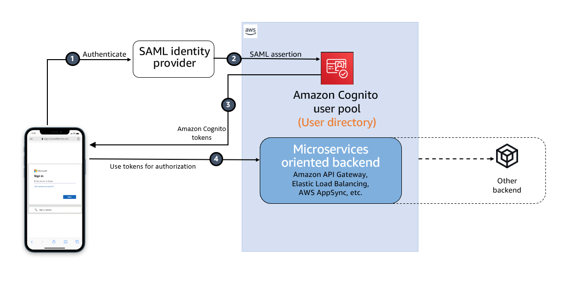
Figure 1: High-level diagram for SAML IdP-initiated authentication flow in a web or mobile app
As shown in Figure 1, the high-level flow diagram of an application with federated authentication typically involves the following steps:
- An enterprise user opens their SSO portal and signs in. This usually opens a portal with several applications that the user has access to. When the user selects an Amazon Cognito protected application from their SSO portal, an IdP-initiated SSO flow is initiated.
- When the user launches an application from the SSO portal, Entra ID sends a SAML assertion to the Cognito endpoint to federate the user.
- Amazon Cognito validates the SAML assertion and creates the user in Cognito if this is first-time federation for the user or updates the user’s record if user has signed in before from this IdP. Cognito then generates an authorization code and redirects the user to the application URL with this authorization code. The application exchanges the authorization code for tokens from the Cognito token endpoint.
- After the application has tokens, it uses them to authorize access within the application stack as needed.
The SAML response contains claims or assertions that contain user-specific data. The SAML response is transferred over HTTPS to protect confidentiality of the data, but you can also enable encryption to further protect the confidentiality of transferred user information. This enables trusted parties who have the decryption key to decrypt the data. It protects the confidentiality of the data after it’s received by the SP.
Setting up SAML federation between Amazon Cognito and Entra ID
To set up SAML federation and use IdP-initiated SSO, you will complete the following steps:
- Create an Amazon Cognito user pool.
- Create an app client in the Cognito user pool.
- Add Cognito as an enterprise application in Entra ID.
- Add Entra ID as the SAML IdP and enable IdP-initiated SSO in Cognito.
- Add the newly created SAML IdP to your user pool app client.
- Enable encrypting the SAML response.
- Add RelayState in Entra ID SAML SSO.
Prerequisites
To implement the solution, you must have the necessary permissions to perform these tasks in Azure portal and in your AWS account.
Step 1: Create an Amazon Cognito user pool
Create a new user pool in Amazon Cognito with the default settings. Make a note of the user pool ID, for example, us-east-1_abcd1234. You will need this value for the next steps.
Add a domain name to user pool
The Cognito user pool’s hosted UI can be used as the OAuth 2.0 authorization server with a customizable web interface for sign-up and sign-in. Cognito OAuth 2.0 endpoints are accessible from a domain name that must be added to the user pool. There are two options for adding a domain name to a user pool. You can either use a Cognito domain or a domain name that you own. This solution uses a Cognito domain, which will look like the following:
https://<yourDomainPrefix>.auth.<aws-region>.amazoncognito.com
To add a domain name to a user pool:
- In the AWS Management Console for Amazon Cognito, navigate to the App integration tab for your user pool.
- On the right side of the pane, choose Actions and select Create Cognito domain.

Figure 2: Create a Cognito domain
- Enter an available domain prefix (for example example-corp-prd) to use with the Cognito domain.
Figure 3: Add a domain prefix
- Choose Create Cognito domain.


Step 2: Create an app client in the Cognito user pool
Before you can use Amazon Cognito in your web application, you must register your app with Amazon Cognito as an app client. The IdP-initiated SAML flow can’t be enabled on one app client with the other SP-initiated authentication SAML IdPs or social IdPs. IdP-initiated SAML introduces additional risks that other SSO providers aren’t subject to. For example, it’s not possible to add a state parameter, which is usually used for cross-site request forgery (CSRF) mitigation. Because of this, you can’t add IdPs that aren’t SAML, including the user pool itself, to an app client that uses a SAML provider with IdP-initiated SSO.
To create an app client:
- In the Amazon Cognito console, navigate to the App integration tab for the same user pool and locate App clients. Choose Create an app client.
- Select an Application type. For this example, create a public client.
- Enter an App client name.
- Choose Don’t generate client secret.
- Keep the rest of the settings as default.
- Under Hosted UI settings, add Allowed callback URLs for your app client. This is where you will be directed after authentication.
- Choose Authorization code grant for OAuth 2.0 grant types.
- You can keep the remaining configuration as default and choose Create app client.
After the app client is successfully created, capture the app client ID from the App integration tab of the user pool.
Prepare information for the Entra ID setup
Prepare the Identifier (Entity ID) and Reply URL, which are required to add Amazon Cognito as an enterprise application in Entra ID (Step 3).
Create values for Identifier (Entity ID) and Reply URL according to the following formats:
For Identifier (Entity ID), the format is:
urn:amazon:cognito:sp:<yourUserPoolID>
For example: urn:amazon:cognito:sp:us-east-1_abcd1234
For Reply URL, the format is:
https://<yourDomainPrefix>.auth.<aws-region>.amazoncognito.com/saml2/idpresponse
For example: https://example-corp-prd.auth.us-east-1.amazoncognito.com/saml2/idpresponse
The reply URL is the endpoint where Entra ID will send the SAML assertion to Amazon Cognito during user authentication.
For more information, see Adding SAML identity providers to a user pool.
Step 3: Add Amazon Cognito as an enterprise application in Entra ID
With the user pool and app client created and the information for Entra ID prepared, you can add Amazon Cognito as an application in Entra ID. To complete this step, you will add Cognito as an enterprise application and set up SSO.
To add Cognito as an enterprise application
- Sign in to the Azure portal.
- In the search box, search for the service Microsoft Entra ID.
- In the left sidebar, select Enterprise applications.
- Choose New application.
- On the Browse Microsoft Entra Gallery page, choose Create your own application.

Figure 4: Create an application in Entra ID
- Under What’s the name of your app?, enter a name for your application and select Integrate any other application you don’t find in the gallery (Non-gallery), as shown in Figure 4. Choose Create.
- It will take few seconds for the application to be created in Entra ID, and then you should be redirected to the Overview page for the newly added application.

To set up SSO using SAML:
- On the Getting started page, in the Set up single sign on tile, choose Get started, as shown in Figure 5.

Figure 5: Choose Set up single sign-on in Getting Started
- On the next screen, select SAML.
- In the middle pane under Set up Single Sign-On with SAML, in the Basic SAML Configuration section, choose the edit icon.
- In the right pane under Basic SAML Configuration, replace the default Identifier ID (Entity ID) with the identifier (entity ID) you created in Step 2. Replace Reply URL (Assertion Consumer Service URL) with the reply URL you created in Step 2.
Figure 6: Add the identifier (entity ID) and reply URL
- Now go to Attributes & Claims and note the claims, as shown in Figure 7. You’ll need these when creating attribute mapping in Amazon Cognito.
Figure 7: Entra ID Attributes & Claims
- Scroll down to the SAML Certificates section and copy the App Federation Metadata Url by choosing the copy into clipboard icon. Make a note of this URL to use in the next step.
Figure 8: Copy SAML metadata URL from Entra ID


Step 4: Add Entra ID as SAML IdP in Amazon Cognito
In this step, you’ll add Entra ID as a SAML IdP to your user pool and download the signing and encryption certificates.
To add the SAML IdP:
- In the Amazon Cognito console, navigate to the Sign-in experience tab of the same user pool. Locate Federated identity provider sign-in and choose Add an Identity provider.
- Choose a SAML IdP.
- Enter a Provider name, for example, EntraID.
- Under IdP-initiated SAML sign-in, choose Accept SP-initiated and IdP-initiated SAML assertions.
- Under Metadata document source, enter the metadata document endpoint URL you captured in Step 3.
- (Optional) Under SAML signing and encryption, select Require encrypted SAML assertion from this provider.
Enable Required encrypted SAML assertion from this provider only if you can turn on token encryption in the Entra ID application. See Step 6.
- Under Map attributes between your SAML provider and your user pool to map SAML provider attributes to the user profile in your user pool. Include your user pool required attributes in your attribute map.
For example, when you choose User pool attribute email, enter the SAML attribute name as it appears in the SAML assertion from your IdP. In our case it will be http://schemas.xmlsoap.org/ws/2005/05/identity/claims/emailaddress.
Figure 9: Enter the SAML attribute name
- Choose Add identity provider.

After the IdP has been created, you can navigate to the recently added EntraID IdP in the user pool for downloading the SAML signing and encryption certificate. These certificates must be imported into the Entra ID enterprise application.
To download the certificates
- To download the SAML signing certificate, Choose View signing certificate and Download as .crt
- To download the SAML encryption certificate, Choose View encryption certificate and Download as .crt.
Step 5: Add the newly created SAML IdP to your user pool app client
Before you can use Amazon Cognito in your web application, you must add the SAML IdP created in Step 4 to your app client.
To add the SAML IdP:
- In the Amazon Cognito console, navigate to the App integration tab for the same user pool and locate App clients.
- Choose the app client you created in Step 2.
- Locate the Hosted UI section and choose Edit.
- Under Identity providers, select the identity provider you created in Step 4 and choose Save changes.

Figure 10: Enabling the Entra ID SAML identity provider in the Cognito app client

At this stage, the Amazon Cognito OAuth 2.0 server is up and running and the web interface is accessible and ready to use. You can access the Cognito hosted UI from your app client using the Cognito console to test it further.
Step 6: Enable encrypting the SAML response in EntraID
For additional security and privacy of user data, enable encrypting the SAML response. Amazon Cognito and your IdP can establish confidentiality in SAML responses when users sign in and sign out. Cognito assigns a public-private RSA key pair and a certificate to each external SAML provider that you configure in your user pool. You will use the SAML encryption certificate downloaded in step 4.
To enable encrypting the SAML response:
- Navigate to your Enterprise application in Entra ID and in the left menu, under Security, select Token encryption.
- Import the SAML encryption certificate you have already downloaded in step 4.
Figure 11: Import the Cognito encryption certificate to Entra ID
- After the certificate is imported, it’s inactive by default. To activate it, right-click on the certificate and select Activate token encryption certificate. This enables the encrypted SAML response.
Figure 12: Activate the token encryption certificate in Entra ID


Step 7: Add RelayState in Entra ID SAML SSO
A RelayState parameter is required when using SAML IdP-initiated authentication flow. Set this up in Entra ID for the Amazon Cognito user pool and the enabled app client ID.
To add RelayState in Entra ID SAML SSO:
- Sign in to the Azure portal and open the enterprise application created in Step 3.
- In the left sidebar, choose Single sign-on.
- In the middle pane under Set up Single Sign-On with SAML, in the Basic SAML Configuration section, choose the edit icon.
- In the right pane under Basic SAML Configuration, apply the value as the format below to the Relay State (Optional) field.
- Replace <IDProviderName> with the name you previously used for ID provider.
- Replace <ClientId> with the app client’s ClientID created in Step 2.
- Replace <ecallbackURL> with the URL of your web application that will receive the authorization code. It must be an HTTPS endpoint, except for in a local development environment where you can use http://localhost:PORT_NUMBER.
For example:
Figure 13: Set RelayState in Entra ID single sign-on

Test the IdP-initiated flow
Next, do a quick test to check if everything is configured properly.
- Sign in to the Azure portal and open the Enterprise application created in Step 3.
- In the left sidebar, choose Users and groups.
- On the right side, choose Add user/group. This will show the Add Assignment page.
- From the left side of the page, choose None Selected .
- Select a user from the right of the screen and follow the prompt to assign the user for this application.
- Once the user is assigned successfully, open https://www.microsoft365.com/apps and sign in as the assigned user.
- After you are signed in, choose the application icon registered as the IdP-initiated SSO.

Figure 14: Testing IdP-initiated SSO from an Office 365 application
- The application will start the IdP-initiated authentication flow and the user will be redirected to the application as a signed-in user.

Signing an authentication request in case of SP-initiated flow
The preceding authentication flow that you tested uses IdP-initiated SSO. If you’re using an SP-initiated flow, you can enable signing of the SAML request that is sent from the SP (Amazon Cognito) to the IdP (Entra ID) for additional security and integrity of communication between them.
You can enable the authentication request signing in Cognito while creating the IdP or by updating your existing IdP.
To enable signing of the SAML request:
- In the Amazon Cognito console, when you create or edit your SAML identity provider, under SAML signing and encryption, select the box Sign SAML requests to this provider and choose Save changes.

Figure 15: Enabling signing SAML request
- Sign in to the Azure portal and access your Entra ID enterprise application. Go to Set up single sign on and edit Verification certificates (optional).
- Select the checkbox Require verification certificates and upload the Cognito user pool SAML signing certificate already downloaded in Step 4 with a .cer file extension. You must convert the .crt file to a .cer file because Entra ID requires a verification certificate in a .cer extension.

To convert the .crt certificate extension to .cer:
- Right-click the .crt file and choose Open.
- Navigate to the Details tab.
- Select Copy to File… and choose Next.
- Select Base-64 encoded X.509 (.CER) and choose Next.
- Give your export file a name (for example, Entra ID.cer) and choose Save.
- Choose Next.
- Confirm the details and choose Finish.
Test the SP-initiated flow
Next, do a quick test to check if everything is configured properly.
- In the Amazon Cognito console, navigate to the App integration tab for the same user pool and locate App clients.
- Choose the app client you created in Step 2.
- Locate the Hosted UI section and choose View Hosted UI.
- From the hosted UI, authenticate yourself using Entra ID as the identity provider.
- After authentication is completed successfully, you will be redirected to the callback URL you configured in your app client with the authorization code.
If you capture the SAML request, you will see that Amazon Cognito is sending a cryptographic signature with the signing certificate in the SAML request to the IdP, and the IdP will match the cryptographic signature with the uploaded certificate to ensure the integrity of the request.
Conclusion
In this post, you learned the benefits of using IdP-initiated single sign-on. It helps centralize administration and lowers dependency on service provider applications. Also, you learned how to integrate an Amazon Cognito user pool with Microsoft Entra ID as an external SAML IdP using IdP-initiated SSO so your users can use their corporate ID to sign in to web or mobile applications. Also, you learned about how to enable signed authentication requests when using an SP-initiated flow and encrypting SAML responses for additional security between Cognito and the SAML IdP.
If you have feedback about this post, submit comments in the Comments section below. If you have questions about this post, contact AWS Support.
Want more AWS Security news? Follow us on Twitter.


 Ravi Animi is a senior product leader in the Amazon Redshift team and manages several functional areas of the Amazon Redshift cloud data warehouse service, including spatial analytics, streaming analytics, query performance, Spark integration, and analytics business strategy. He has experience with relational databases, multidimensional databases, IoT technologies, storage and compute infrastructure services, and more recently, as a startup founder in the areas of artificial intelligence (AI) and deep learning, computer vision, and robotics.
 Ioanna Tsalouchidou is a software development engineer in the Amazon Redshift team focusing on spatial analytics and query processing. She holds a PhD in graph algorithms from UPF Spain and a Masters in distributed systems and computing from KTH Sweden and UPC Spain.
 Hinnerk Gildhoff is a senior engineering leader in the Amazon Redshift team leading query processing, spatial analytics, materialized views, autonomics, query languages and more. Prior to joining Amazon, Hinnerk spent over a decade as both an engineer and a manager in the field of in-memory and cluster computing, specializing in building databases and distributed systems.
 Javier de la Torre is founder and Chief Strategy Officer of CARTO, has been instrumental in advancing the geospatial industry. At CARTO, he’s led innovations in location intelligence. He also serves on the Open Geospatial Consortium board, aiding in the development of standards like geoparquet. Javier’s commitment extends to environmental causes through his work with Tierra Pura, focusing on climate change and conservation, demonstrating his dedication to using data for global betterment.