This week, Metasploit community member h00die added the second of two modules targeting Rancher instances. These modules each leak sensitive information from vulnerable instances of the application which is intended to manage Kubernetes clusters. These are a great addition to Metasploit’s coverage for testing Kubernetes environments.
PAN-OS RCE
Metasploit also released an exploit for the unauthenticated RCE in PAN-OS that has been receiving a lot of attention recently. This vulnerability is an unauthenticated file creation that can be leveraged to trigger the execution of remote commands. See Rapid7’s analysis on AttackerKB for an in depth explanation of the root cause.
New module content (8)
Rancher Authenticated API Credential Exposure
Authors: Florian Struck, Marco Stuurman, and h00die
Type: Auxiliary
Pull request: #18956 contributed by h00die
Path: gather/rancher_authenticated_api_cred_exposure
AttackerKB reference: CVE-2021-36782
Description: This adds an exploit for CVE-2021-36782, a vulnerability which can be leveraged by an authenticated attacker to leak API credentials from an affected Rancher instance.
Description: A web page exists that can be reached without authentication that contains a hash that can be used to determine the approximate version of gitlab running on the endpoint. This PR enhances our current GitLab fingerprinting capabilities to include the aforementioned technique.
Apache Solr Backup/Restore APIs RCE
Authors: jheysel-r7 and l3yx
Type: Exploit
Pull request: #19046 contributed by jheysel-r7
Path: linux/http/apache_solr_backup_restore
AttackerKB reference: CVE-2023-50386
Description: Adds apache_solr_backup_restore module, taking advantage of a Unrestricted Upload of File with Dangerous Type vulnerability, allowing the user to gain a session in an Apache Solr instance for remote code execution.
Authors: remmons-r7 and sfewer-r7
Type: Exploit
Pull request: #19101 contributed by remmons-r7
Path: linux/http/panos_telemetry_cmd_exec
AttackerKB reference: CVE-2024-3400
Description: This adds an exploit module for https://security.paloaltonetworks.com/CVE-2024-3400, affecting PAN-OS GlobalProtect Gateway and GlobalProtect Portal deployments with the default telemetry service enabled.
GitLens Git Local Configuration Exec
Authors: Paul Gerste and h00die
Type: Exploit
Pull request: #18997 contributed by h00die
Path: multi/fileformat/gitlens_local_config_exec
AttackerKB reference: CVE-2023-46944
Description: This adds a FileFormat exploit for VSCode. The VSCode extension GitLens by GitKraken before v.14.0.0 allows an untrusted workspace to execute git commands. A repo may include its own .git folder including a malicious config file to execute arbitrary code.
Authors: h00die-gr3y [email protected] and usd Herolab
Type: Exploit
Pull request: #19005 contributed by h00die-gr3y
Path: multi/http/gambio_unauth_rce_cve_2024_23759
AttackerKB reference: CVE-2024-23759
Description: This adds a module for a Remote Code Execution vulnerability in Gambio Online Webshop version 4.9.2.0 and lower allows remote attackers to run arbitrary commands via unauthenticated HTTP POST request.
FortiNet FortiClient Endpoint Management Server FCTID SQLi to RCE
Authors: James Horseman, Spencer McIntyre, Zach Hanley, and jheysel-r7
Type: Exploit
Pull request: #19082 contributed by jheysel-r7
Path: windows/http/forticlient_ems_fctid_sqli
AttackerKB reference: CVE-2023-48788
Description: Adds windows/http/forticlient_ems_fctid_sqli module that takes advantage of a SQLi injection vulnerability in FortiNet FortiClient EMS.
Enhancements and features (11)
#17294 from adfoster-r7 – This adds a new EVENT_DEPENDENT value for module reliability metadata.
#18723 from jvoisin – A web page exists that can be reached without authentication that contains a hash that can be used to determine the approximate version of gitlab running on the endpoint. This PR enhances our current GitLab fingerprinting capabilities to include the aforementioned technique.
#18914 from dotslashsuperstar – This PR adds functionality so that CVE and URL references will be imported from an OpenVAS XML report by default. DNF-CERT and CERT-BUND references can also be collected by sending additional flags to the db_import command.
#19054 from zgoldman-r7 – Adds NText column parsing to MSSQL modules.
#19066 from sjanusz-r7 – Adds automated tests for multiple SMB modules.
#19078 from dwelch-r7 – Fixes a crash in the modules/auxiliary/gather/ldap_query.rb module when running queries from a file.
#19080 from cgranleese-r7 – Adds architecture and platform detection for PostgreSQL sessions.
#19086 from nrathaus – Update Metasploit’s RPC to expose module’s default_options metadata.
#19112 from zgoldman-r7 – Adds architecture and platform detection for MSSQL sessions.
#19122 from h00die – Adds additional reliability metadata to exploits/linux/local/vcenter_java_wrapper_vmon_priv_esc.
Bugs fixed (6)
#19079 from nrathaus – Fixes an issue were the password_spray module option was being ignored.
#19089 from adfoster-r7 – This PR fixes a bug where a user might get an unexpected NoMethodError running the linux/local/exim4_deliver_message_priv_esc module.
#19111 from zeroSteiner – This PR fixes a bug where a user can specify an invalid payload architecture for a given exploit target. Previously, it was not possible to tab-complete an invalid payload, but this enforces the architecture limitations with a run-time exception before sending the exploit.
#19113 from adfoster-r7 – Fixes a regression that caused Metasploit to leak memory, and sometimes crash.
#19114 from zeroSteiner – This PR fixes several instances where we we pass nil values rather than the types expected, causing crashes and stack traces in LDAP-related modules.
#19129 from nrathaus – This fixes a bug where the notes command included an example which contained a flag that was not supported.
Documentation added (1)
#19088 from adfoster-r7 – This PR adds documentation for running and writing Metasploit’s unit tests.
You can always find more documentation on our docsite at docs.metasploit.com.
Get it
As always, you can update to the latest Metasploit Framework with msfupdate
and you can get more details on the changes since the last blog post from
GitHub:
To enable your workforce users for analytics with fine-grained data access controls and audit data access, you might have to create multiple AWS Identity and Access Management (IAM) roles with different data permissions and map the workforce users to one of those roles. Multiple users are often mapped to the same role where they need similar privileges to enable data access controls at the corporate user or group level and audit data access.
AWS IAM Identity Center enables centralized management of workforce user access to AWS accounts and applications using a local identity store or by connecting corporate directories via identity providers (IdPs). IAM Identity Center now supports trusted identity propagation, a streamlined experience for users who require access to data with AWS analytics services.
Amazon EMR Studio is an integrated development environment (IDE) that makes it straightforward for data scientists and data engineers to build data engineering and data science applications. With trusted identity propagation, data access management can be based on a user’s corporate identity and can be propagated seamlessly as they access data with single sign-on to build analytics applications with Amazon EMR (EMR Studio and Amazon EMR on EC2).
AWS Lake Formation allows data administrators to centrally govern, secure, and share data for analytics and machine learning (ML). With trusted identity propagation, data administrators can directly provide granular access to corporate users using their identity attributes and simplify the traceability of end-to-end data access across AWS services. Because access is managed based on a user’s corporate identity, they don’t need to use database local user credentials or assume an IAM role to access data.
In this post, we show how to bring your workforce identity to EMR Studio for analytics use cases, directly manage fine-grained permissions for the corporate users and groups using Lake Formation, and audit their data access.
Solution overview
For our use case, we want to enable a data analyst user named analyst1 to use their own enterprise credentials to query data they have been granted permissions to and audit their data access. We use Okta as the IdP for this demonstration. The following diagram illustrates the solution architecture.
This architecture is based on the following components:
Okta is responsible for maintaining the corporate user identities, related groups, and user authentication.
IAM Identity Center connects Okta users and centrally manages their access across AWS accounts and applications.
Lake Formation provides fine-grained access controls on data directly to corporate users using trusted identity propagation.
EMR Studio is an IDE for users to build and run applications. It allows users to log in directly with their corporate credentials without signing in to the AWS Management Console.
For this setup, we have created two users, analyst1 and engineer1, and assigned them to the corresponding Okta application. You can validate the integration is working by navigating to the Users page on the IAM Identity Center console, as shown in the following screenshot. Both enterprise users from Okta are provisioned in IAM Identity Center.
The following exact users will not be listed in your account. You can either create similar users or use an existing user.
Each provisioned user in IAM Identity Center has a unique user ID. This ID does not originate from Okta; it’s created in IAM Identity Center to uniquely identify this user. With trusted identity propagation, this user ID will be propagated across services and also used for traceability purposes in CloudTrail. The following screenshot shows the IAM Identity Center user matching the provisioned Okta user analyst1.
Choose the link under AWS access portal URL and log in with the analyst1 Okta user credentials that are already assigned to this application.
If you are able to log in and see the landing page, then all your configurations up to this step are set correctly. You will not see any applications on this page yet.
Set up EMR Studio
In this step, we demonstrate the actions needed from the data lake administrator to set up EMR Studio enabled for trusted identity propagation and with IAM Identity Center integration. This allows users to directly access EMR Studio with their enterprise credentials.
Note: All Amazon S3 buckets (created after January 5, 2023) have encryption configured by default (Amazon S3 managed keys (SSE-S3)), and all new objects that are uploaded to an S3 bucket are automatically encrypted at rest. To use a different type of encryption, to meet your security needs, please update the default encryption configuration for the bucket. See Protecting data for server-side encryption for further details.
On the Amazon EMR console, choose Studios in the navigation pane under EMR Studio.
Choose Create Studio.
For Setup options¸ select Custom.
For Studio name, enter a name (for this post, emr-studio-with-tip).
For S3 location for Workspace storage, select Select existing location and enter an existing S3 bucket (if you have one). Otherwise, select Create new bucket.
For Service role to let Studio access your AWS resources, choose View permissions details to get the trust and IAM policy information that is needed and create a role with those specific policies in IAM. In this case, we create a new role called emr_tip_role.
For Service role to let Studio access your AWS resources, choose the IAM role you created.
For Workspace name, enter a name (for this post, studio-workspace-with-tip).
For Authentication, select IAM Identity Center.
For User role¸ you can create a new role or choose an existing role. For this post, we choose the role we created (emr_tip_role).
To use the same role, add the following statement to the trust policy of the service role:
Select Enable trusted identity propagation to allow you to control and log user access across connected applications.
For Choose who can access your application, select All users and groups.
Later, we restrict access to resources using Lake Formation. However, there is an option here to restrict access to only assigned users and groups.
In the Networking and security section, you can provide optional details for your VPC, subnets, and security group settings.
Choose Create Studio.
On the Studios page of the Amazon EMR console, locate your Studio enabled with IAM Identity Center.
Copy the link for Studio Access URL.
Enter the URL into a web browser and log in using Okta credentials.
You should be able to successfully sign in to the EMR Studio console.
Create an AWS Identity Center enabled security configuration for EMR clusters
EMR security configurations allow you to configure data encryption, Kerberos authentication, and Amazon S3 authorization for the EMR File System (EMRFS) on the clusters. The security configuration is available to use and reuse when you create clusters.
To integrate Amazon EMR with IAM Identity Center, you need to first create an IAM role that authenticates with IAM Identity Center from the EMR cluster. Amazon EMR uses IAM credentials to relay the IAM Identity Center identity to downstream services such as Lake Formation. The IAM role should also have the respective permissions to invoke the downstream services.
Create a role (for this post, called emr-idc-application) with the following trust and permission policy. The role referenced in the trust policy is the InstanceProfile role for EMR clusters. This allows the EC2 instance profile to assume this role and act as an identity broker on behalf of the federated users.
Upload my-certs.zip to an S3 location that will be used to create the security configuration.
The EMR service role should have access to the S3 location. The key allows access to the issuer’s EMR cluster instances in the us-west-2 Region as specified by the *.us-west-2.compute.internal domain name as the common name. You can change this to the Region your cluster is in.
You can view the security configuration on the Amazon EMR console.
Create a Service Catalog product template to create EMR clusters
EMR Studio with trusted identity propagation enabled can only work with clusters created from a template. Complete the following steps to create a product template in Service Catalog:
On the Service Catalog console, choose Portfolios under Administration in the navigation pane.
Choose Create portfolio.
Enter a name for your portfolio (for this post, EMR Clusters Template) and an optional description.
Choose Create.
On the Portfolios page, choose the portfolio you just created to view its details.
On the Products tab, choose Create product.
For Product type, select CloudFormation.
For Product name, enter a name (for this post, EMR-7.0.0).
Use the security configuration IdentityCenterConfiguration-with-lf-tip you created in previous steps with the appropriate Amazon EMR service roles.
Choose Create product.
The following is an example CloudFormation template. Update the account-specific values for SecurityConfiguration, JobFlowRole, ServiceRole, LogUri, Ec2KeyName, and Ec2SubnetId. We provide a sample Amazon EMR service role and trust policy in Appendix A at the end of this post.
Trusted identity propagation is supported from Amazon EMR 6.15 onwards. For Amazon EMR 6.15, add the following bootstrap action to the CloudFormation script:
The portfolio now should have the EMR cluster creation product added.
Grant the EMR Studio role emr_tip_role access to the portfolio.
Grant Lake Formation permissions to users to access data
In this step, we enable Lake Formation integration with IAM Identity Center and grant permissions to the Identity Center user analyst1. If Lake Formation is not already enabled, refer to Getting started with Lake Formation.
To use Lake Formation with Amazon EMR, create a custom role to register S3 locations. You need to create a new custom role with Amazon S3 access and not use the default role AWSServiceRoleForLakeFormationDataAccess. Additionally, enable external data filtering in Lake Formation. For more details, refer to Enable Lake Formation with Amazon EMR.
Complete the following steps to manage access permissions in Lake Formation:
On the Lake Formation console, choose IAM Identity Center integration under Administration in the navigation pane.
Lake Formation will automatically specify the correct IAM Identity Center instance.
Choose Create.
You can now view the IAM Identity Center integration details.
For this post, we have a Marketing database and a customer table on which we grant access to our enterprise user analyst1. You can use an existing database and table in your account or create a new one. For more examples, refer to Tutorials.
The following screenshot shows the details of our customer table.
On the Lake Formation console, choose Data lake permissions under Permissions in the navigation pane.
Choose Grant.
Select Named Data Catalog resources.
For Databases, choose your database (marketing).
For Tables, choose your table (customer).
For Table permissions, select Select and Describe.
For Data permissions, select All data access.
Choose Grant.
The following screenshot shows a summary of permissions that user analyst1 has. They have Select access on the table and Describe permissions on the databases.
Test the solution
To test the solution, we log in to EMR Studio as enterprise user analyst1, create a new Workspace, create an EMR cluster using a template, and use that cluster to perform an analysis. You could also use the Workspace that was created during the Studio setup. In this demonstration, we create a new Workspace.
You need additional permissions in the EMR Studio role to create and list Workspaces, use a template, and create EMR clusters. For more details, refer to Configure EMR Studio user permissions for Amazon EC2 or Amazon EKS. Appendix B at the end of this post contains a sample policy.
When the cluster is available, we attach the cluster to the Workspace and run queries on the customer table, which the user has access to.
User analyst1 is now able to run queries for business use cases using their corporate identity. To open a PySpark notebook, we choose PySpark under Notebook.
When the notebook is open, we run a Spark SQL query to list the databases:
%%sql
show databases
In this case, we query the customer table in the marketing database. We should be able to access the data.
%%sql
select * from marketing.customer
Audit data access
Lake Formation API actions are logged by CloudTrail. The GetDataAccess action is logged whenever a principal or integrated AWS service requests temporary credentials to access data in a data lake location that is registered with Lake Formation. With trusted identity propagation, CloudTrail also logs the IAM Identity Center user ID of the corporate identity who requested access to the data.
The following screenshot shows the details for the analyst1 user.
Choose View event to view the event logs.
The following is an example of the GetDataAccess event log. We can trace that user analyst1, Identity Center user ID c8c11390-00a1-706e-0c7a-bbcc5a1c9a7f, has accessed the customer table.
In this post, we demonstrated how to set up and use trusted identity propagation using IAM Identity Center, EMR Studio, and Lake Formation for analytics. With trusted identity propagation, a user’s corporate identity is seamlessly propagated as they access data using single sign-on across AWS analytics services to build analytics applications. Data administrators can provide fine-grained data access directly to corporate users and groups and audit usage. To learn more, see Integrate Amazon EMR with AWS IAM Identity Center.
About the Authors
Pradeep Misra is a Principal Analytics Solutions Architect at AWS. He works across Amazon to architect and design modern distributed analytics and AI/ML platform solutions. He is passionate about solving customer challenges using data, analytics, and AI/ML. Outside of work, Pradeep likes exploring new places, trying new cuisines, and playing board games with his family. He also likes doing science experiments with his daughters.
Deepmala Agarwal works as an AWS Data Specialist Solutions Architect. She is passionate about helping customers build out scalable, distributed, and data-driven solutions on AWS. When not at work, Deepmala likes spending time with family, walking, listening to music, watching movies, and cooking!
Abhilash Nagilla is a Senior Specialist Solutions Architect at Amazon Web Services (AWS), helping public sector customers on their cloud journey with a focus on AWS analytics services. Outside of work, Abhilash enjoys learning new technologies, watching movies, and visiting new places.
Appendix A
Sample Amazon EMR service role and trust policy:
Note: This is a sample service role. Fine grained access control is done using Lake Formation. Modify the permissions as per your enterprise guidance and to comply with your security team.
Note: This is a sample service role. Fine grained access control is done using Lake Formation. Modify the permissions as per your enterprise guidance and to comply with your security team.
Продукти: 1 кг брашно, 5 яйца, 200 г захар, 1/2 кг мляко (рецептата е стара, млякото се мери в килограми, премерих го на електронна везна), 40 г прясна или 20 г суха мая (от бързодействащата), ванилия – колкото обичате, 200 г масло.
И двете ми баби смятаха козунаците за висш пилотаж и не се престрашаваха да месят, само разказваха за своите баби и майки, които месили, преди да се появят „купешките“. По патос и драматизъм разказите им се равняваха на приказки. В тях бабите бореха козунаци, побеждаваха ги, биеха ги в масата по двеста пъти и най-накрая козунаците се появяваха съвършени, както роклята на царкинята от ореховата черупка – красиво зачервени и обсипани със скъпоценни камъни от захар.
Снимка: Йоанна Елми
Започнах да правя опити за козунак в студентските си години. След това дойде и 2020-та, когато много от нас преоткриха удоволствието от забавеното време, което позволява да почакаш нещо да втаса. Козунакът постепенно стана ритуал, повод за мислене на близостта (особено след преместването ми в Щатите) и връзка с онзи Великден, който помня от дете.
Пресейте брашното и в него направете кладенче. Смесете маята с малко от млякото и оставете настрана.
През годините с няколко близки приятели изпробвахме най-различни рецепти. При търсене на „козунак“ Google изплюва хиляди, всяка от които е за най-добрия козунак, с най-многото конци, най-автентичния и т.н. Към тях добавяме и многобройни статии, които дават често взаимно противоречащи си съвети как да се избере най-добрият козунак от магазина. Към пробваните козунаци спадат и изядените изобщо, без ние да сме ги приготвили: сред тях са творенията на поне пет различни баби от най-различни краища на страната, няколко известни (хипстърски) софийски пекарни, няма как да пропусна и козунаците, раздадени от ПП ГЕРБ в ж.к. „Тракия“, гр. Пловдив, преди парламентарните избори през 2013 г. (съвсем истинска история, но да не си разваляме празника). Чак тази година обаче открих Рецептата за козунак – такъв, какъвто трябва да е. Споделям я от книгата с рецепти на прабаба ми и баба ми, учебника по домакинство „Календар по готварство“ от 1937 г., допълнена с обяснения. И всичко останало, което ражда търпението да направиш хубав козунак.
Когато маята шупне, изсипете я при брашното в кладенчето и размесете леко. Оставете настрана. Разтопете маслото и го оставете да поизстине. Разбийте яйцата в купа, докато станат на пяна, около 5–7 минути с миксера на висока степен. Добавете захарта и продължете да смесвате с миксера, докато не се получи хомогенна смес с много балончета.
На пръв поглед козунакът не е нещо специално – меси се в Румъния, Молдова, Сърбия и Гърция, по състав и структура е братовчед на италианския панетоне, на френския бриош. Подобно на новогодишната баница или обредните питки, у нас козунакът има особен статус не поради състава си, а поради историята, която може да разкаже за себе си, и историите, които оставя в нас. От ранното детство ароматът му е предвестник на пролет и слънце, по-дълги дни и повече игри навън, спомен за онова стоене до късно и обикаляне около църквата, шарените яйца, дали ти ще си с бореца тази година… Куполът на храм-паметника „Св. Троица“ в едноименния квартал, където съм израснала, се виждаше през все още крехката пролетна зеленина и в годините, когато нямахме възможност да отидем до църквата по една или друга причина, гледах от прозореца как свещите трептят в мрака и след това се пръсват по алеите на парка обратно към домовете. Със сигурност си въобразявам, но тогава целият квартал ухаеше на козунаци.
Казваме къде шеговито, къде с искрено порицание, че българинът е християнин, който влиза в църква само по Коледа и Великден. Струва ми се обаче, че козунакът дава повод за аргумента, че не традициите принадлежат на празниците, а празниците – на традициите. Символиката на пролетното равноденствие е една и съща навсякъде: възраждане или възкресение, ново начало, събуждане на природата, подготовка за активна земеделска работа и т.н. Правенето на хляб, носенето на огън, приготвянето на храна със специфична символика, празнуването заедно с членовете на общността не са част от църковния канон, а са набор от ритуали, свързани със символиката на равноденствието. Това прави козунака по-скоро част от човешкото, което създава ритуал от нужда за близост до другите и природата извън всякаква намеса на религиозното или идеологическото, които го усвояват впоследствие. Историята не е само в ритуала. Всяка рецепта разказва история – както колективна, така и лична. Голяма и малка.
Добавете и поизстиналото масло. Продължете да биете с миксера, докато не стане светла хомогенна смес с много балончета. Добавете и млякото, като отново разбъркате по същия начин. Накрая добавете и ванилията.
Снимка: Йоанна Елми
В преиздадения „Календар по готварство“ от 1937 г. рецептите са групирани по месеци, със сезонни продукти, като „са взети под внимание нашите национални традиции за храненето“. Освен това се казва, че продуктите са съобразени със „скромния“ български пазар. Остава да се чудим дали уточнението е било част от оригинала, или е добавено след 1944 г. И двата варианта са възможни – в първия пазарът може да е скромен поради няколкото национални кризи, нестабилната световна икономика на 30-те години или заради бедността, която както тогава, така и сега е ежедневие за много български домакинства. След идването на комунистите нещата не се променят кой знае колко, разменят се само ролите, и то не на всички.
Има и друг вариант за тази скромност – устойчивостта. Рецептите в книгата са със сезонни продукти, максимум между пет и осем съставки на ястие, включително и подправките, които също са местни, плюс задължителните сол и пипер. Не става въпрос само за регионални гозби, има например и виенски десерти, но всичко следва същия принцип. Традиционните рецепти всъщност изглеждат подозрително… зелени.
Изсипете брашното в достатъчно голяма тава или купа. Започнете да добавяте по чаша-две/черпак-два от течната смес, като разбърквате отначало с дървена лъжица, а след като започне да се оформя тесто – с ръце. Добавяйте течността постепенно, докато тестото става все по-хомогенно.
Снимка: Йоанна Елми
Както много българи, живели в XX в., и баба ми и дядо ми жонглираха със задушеното си в индустриализация и урбанизация земеделско наследство и комунистическата оскъдица. Дядо ми до последно разказваше с носталгия как като деца са пасли воловете по безкрайните полета край Търново; баба ми оплакваше „унищожението на българското село от комунистите“. До известна степен и двамата се помиряваха с неизбежното, което щеше да се случи и без абсурдите на диктатурата – откъсването на човека от природата, от малката общност, от бавното живеене, което е световна и ускоряваща се тенденция от близо два века.
Успоредно с работата и децата, а после и с внучката, двамата се грижеха за най-различни зеленчукови и овощни градини, затваряха буркани, гледаха животни за месо, яйца и мляко. Отначало защото по магазините често или не е имало достатъчно, или качеството е било много ниско, а след това – по навик и даже от любов. В този смисъл кухнята ни винаги е била скромна, но никога не ми е хрумвало, че храната, която консумираме, не е вкусна или не ни стига. Напротив – днес доматите и чушките, които гледаха баба ми и дядо ми, се продават на тройни цени и с етикет „био“. И тук изобщо не става дума за соцносталгия.
Градината и животните отнемаха много труд, търпение и ресурси като време и вода за поливане. Време, което все пак са намирали – може би защото не са се карали с никого по цял ден във Facebook. Кухнята им си остана все така простичка.
Ако всичко върви добре, би трябвало да ви остане около 100 – 200 мл течност. Извадете тестото от тавата, поставете го на плот или маса и почнете да добавяте течността постепенно, като оставяте време да поеме в процеса на месене. Тестото ще става все по-гладко, все по-меко и все по-лепкаво, без обаче да лепи върху плота. Малко залепване и разкашкване при добавяне на течността е нормално, но след това тестото трябва отново да се „събере“ и стегне.
Ние, техните наследници, живеем много по-различно. „Консервативното небце“ на българина се променя, опитваме все повече храни, традиционната ни кухня излиза в света, светът влиза у нас. В супермаркетите, независимо дали във Франция, Германия, България, САЩ или Нидерландия, сезонното е само спомен. Тази промяна в храненето е огледало на по-големи промени: безпрецедентна технологична революция и промяна в начина на комуникации, отмирането на индустрията и възходът на сферата на услугите, затварянето на няколко поколения в офиси и градска среда, живот и детство, които преминават пред екрани.
Доста хора в България все още отглеждат някаква част от храната си, но все пак много по-малко от преди. В чужбина обаче има обратна тенденция, особено сред младите – дали заради нарастващата инфлация и високите цени на пресните продукти, дали поради съображения за околната среда, или просто като страничен ефект от пандемията. Културни тенденции като т.нар. cottagecore превръщат подобен начин на живот в своеобразен естетически култ. Разбира се, историята няма как да тръгне назад. Но тези феномени не се появяват случайно. Те са реакция спрямо настоящето.
Тестото е готово, когато започне леко да лепи по плота и стане напълно гладко. Тогава се оставя да втаса – няколко часа на стайна температура, докато удвои обема си, или в хладилника през нощта. Ако втасва в хладилник, тестото трябва да се отпусне няколко часа, преди да се меси втори път.
Изобилието си има цена, особено когато привидно излиза евтино. Авокадото например се контролира от кървави картели и допринася за изсичането на горите в Амазония. Дори когато не става въпрос за такива драстични случаи, съвременното производство на храна допринася за вредните емисии на парникови газове, дестабилизира местните земеделци, поддържа отровни земеделски практики, наводнява пазара с продукти, пълни с пестициди. Проблемите са много и картината е сложна, но това са някои от по-негативните тенденции, които всички слагаме доброволно в чинията си ден след ден.
Все повече хора в т.нар. развит свят боледуват и умират от изобилие и преяждане. Затлъстяването сред децата е сериозен здравен проблем, включително в България. Качеството на храната се влошава не само поради гореизброените причини, а и поради начините на съхранение, често в найлон и пластмаса, от които в храната се просмукват канцерогенни и увреждащи ендокринната система вещества. Всичко това – преди дори да се разградят до микропластмаси, които поглъщаме и които вече се откриват дори в плацентата на бременни жени. Ако отворим обектива още повече, изобилието от продукти почти винаги води до исторически и съвременни колониални и експлоатационни практики. Историята на храната всъщност е сложната история на света, с всичките нюанси на миналото и съвремието.
След като тестото втаса веднъж, се размесва още един път. На този етап се добавят стафиди, шоколад или каквото друго решите да сложите в него. Оформя се както ви харесва – онлайн има множество начини за заплитане на венци, плитки и т.н. Ако решите, може да намажете фитилите с мармалад, преди да ги заплетете. Козунакът се оставя да удвои обема си още веднъж за час-два на стайна температура.
Снимка: Йоанна Елми
Може би от необходимото време и внимание за месене на козунака, което ражда такива потоци на съзнанието, се е родил митът, че той трябва да се удари между двайсет и пет и двеста пъти (в зависимост от източника) в масата. Поглеждайки от време на време към старата книга с рецепти, си давам сметка, че скромност съвсем не е същото като оскъдица или липса. Че традицията изпълнява своя смисъл не когато се използва за напразни обещания за завръщане към миналото, а за осмисляне на настоящето и евентуално на бъдещето.
Кое може да си вземем от това минало? Усещането за време и по-смислената му инвестиция в ежедневното? Излизането от виртуалния свят и връщането в света на допира – до почва, до живот, до тесто, до друг човек? Изкуството търпеливо да омесиш нещо, да положиш усилие, да почакаш процесите да втасат, вместо да търсиш бързите въглехидрати на допамина или агресията? Връщането към споделеното и общността? Осъзнаването, че изобилието е дар тогава, когато не е ежедневие и не се превръща в прекаляване и алчност? И може би, някой ден, доброволното ограничаване на безкрайната консумация в името на едно по-добро бъдеще? Скромност?
Хубавите неща стават бавно – същинското месене ми отне около час. Рецептата е простичка, трябва да се внимава, може да бъде и трудна за изпълнение. Разчита се на помощ от инструкциите, но и на усет, на преценка. Козунакът става мек, пухкав и остава мек за дни напред. Не е нито твърде сладък, нито безвкусен. Усилието, с две думи, си заслужава.
Козунакът се намазва с цяло разбито яйце. Може да се поръси с бадем. Пече се на 175–180 градуса за около 40 минути. След като се извади, се изправя, за да изстине равномерно, или се поставя върху решетка. Яде се топъл, по възможност – с близки. И с благодарност и мисъл за конците на голямата и малката история, от която е направен.
Video playback is undeniably one of the most important features in modern
consumer devices. Yet, surprisingly, users are by and large unaware of the
intricate engineering involved in the compression and decompression of
video data, with codecs being left to find a delicate balance between image
quality, bandwidth, and power consumption. In response to constant
performance pressure, video codecs have become complex and hardware
implementations are now common, but programming these devices is becoming
increasingly difficult and fraught with opportunities for exploitation. I
hope to convey how Rust can help fix this problem.
At the CPU level, a memory model describes, among other things, the amount
of freedom the processor has to reorder memory operations. If low-level
code does not take the memory model into account, unpleasant surprises are
likely to follow. Naturally, different CPUs offer different memory models,
complicating the portability of certain types of concurrent software. To
make life easier, some Arm CPUs offer the ability to emulate the x86 memory
model, but efforts to make that feature available in the kernel are running
into opposition.
Security updates have been issued by Debian (knot-resolver, pdns-recursor, and putty), Fedora (xen), Mageia (editorconfig-core-c, glibc, mbedtls, webkit2, and wireshark), Oracle (buildah), Red Hat (buildah and yajl), Slackware (libarchive), SUSE (dcmtk, openCryptoki, php7, php74, php8, python-gunicorn, python-idna, qemu, and thunderbird), and Ubuntu (cryptojs, freerdp2, nghttp2, and zabbix).
APIs are the key to implementing microservices that are the building blocks of modern distributed applications. Launching a new API involves defining the behavior, implementing the business logic, and configuring the infrastructure to enforce the behavior and expose the business logic. Using OpenAPI, the AWS Cloud Development Kit (AWS CDK), and AWS Solutions Constructs to build your API lets you focus on each of these tasks in isolation, using a technology specific to each for efficiency and clarity.
The OpenAPI specification is a declarative language that allows you to fully define a REST API in a document completely decoupled from the implementation. The specification defines all resources, methods, query strings, request and response bodies, authorization methods and any data structures passed in and out of the API. Since it is decoupled from the implementation and coded in an easy-to-understand format, this specification can be socialized with stakeholders and developers to generate buy-in before development has started. Even better, since this specification is in a machine-readable syntax (JSON or YAML), it can be used to generate documentation, client code libraries, or mock APIs that mimic an actual API implementation. An OpenAPI specification can be used to fully configure an Amazon API Gateway REST API with custom AWS Lambda integration. Defining the API in this way automates the complex task of configuring the API, and it offloads all enforcement of the API details to API Gateway and out of your business logic.
The AWS CDK provides a programming model above the static AWS CloudFormation template, representing all AWS resources with instantiated objects in a high-level programming language. When you instantiate CDK objects in your Typescript (or other language) code, the CDK “compiles” those objects into a JSON template, then deploys that template with CloudFormation. I’m not going to spend a lot of time extolling the many virtues of the AWS CDK here, suffice it to say that the use of programming languages such as Typescript or Python rather than the declarative YAML or JSON allows much more flexibility in defining your infrastructure.
AWS Solutions Constructs is a library of common architectural patterns built on top of the AWS CDK. These multi-service patterns allow you to deploy multiple resources with a single CDK Construct. Solutions Constructs follow best practices by default – both for the configuration of the individual resources as well as their interaction. While each Solutions Construct implements a very small architectural pattern, they are designed so that multiple constructs can be combined by sharing a common resource. For instance, a Solutions Construct that implements an Amazon Simple Storage Service (Amazon S3) bucket invoking a Lambda function can be deployed with a second Solutions Construct that deploys a Lambda function that writes to an Amazon Simple Queue Service (Amazon SQS) queue by sharing the same Lambda function between the two constructs. You can compose complex architectures by connecting multiple Solutions Constructs together, as you will see in this example.
Infrastructure as Code Abstraction Layers
In this article, you will build a robust, functional REST API based on an OpenAPI specification using the AWS CDK and AWS Solutions Constructs.
How it Works
This example is a microservice that saves and retrieves product orders. The behavior will be fully defined by an OpenAPI specification and will include the following methods:
Method
Functionality
Authorization
POST /order
Accepts order attributes included in the request body. Returns the orderId assigned to the new order.
Accepts an orderId as a path parameter. Returns the fully populated order object.
IAM
The architecture implementing the service is shown in the diagram below. Each method will integrate with a Lambda function that implements the interactions with an Amazon DynamoDB table. The API will be protected by IAM authorization and all input and output data will be verified by API Gateway. All of this will be fully defined in an OpenAPI specification that is used to configure the REST API.
The Two Solutions Constructs Making up the Service Architecture
Infrastructure as code will be implemented with the AWS CDK and AWS Solutions Constructs. This example uses 2 Solutions Constructs:
aws-lambda-dynamodb – This construct “connects” a Lambda function and a DynamoDB table. This entails giving the Lambda function the minimum IAM privileges to read and write from the table and providing the DynamoDB table name to the Lambda function code with an environment variable. A Solutions Constructs pattern will create its resources based on best practices by default, but a client can also provide construct properties to override the default behaviors. A client can also choose not to have the pattern create a new resource by providing a resource that already exists.
aws-openapigateway-lambda – This construct deploys a REST API on API Gateway configured by the OpenAPI specification, integrating each method of the API with a Lambda function. The OpenAPI specification is stored as an asset in S3 and referenced by the CloudFormation template rather than embedded in the template. When the Lambda functions in the stack have been created, a custom resource processes the OpenAPI asset and updates all the method specifications with the arn of the associated Lambda function. An API can point to multiple Lambda functions, or a Lambda function can provide the implementation for multiple methods.
In this example you will create the aws-lambda-dynamodb construct first. This construct will create your Lambda function, which you then supply as an existing resource to the aws-openapigateway-lambda constructor. Sharing this function between the constructs will unite the two small patterns into a complete architecture.
Prerequisites
To deploy this example, you will need the following in your development environment:
Typescript 3.8 or later (npm -g install typescript)
AWS CDK 2.82.0 or later (npm install -g aws-cdk && cdk bootstrap)
The cdk bootstrap command will launch an S3 bucket and other resources that the CDK requires into your default region. You will need to bootstrap your account using a role with sufficient privileges – you may require an account administrator to complete that command.
Tip – While AWS CDK. 2.82.0 is the minimum required to make this example work, AWS recommends regularly updating your apps to use the latest CDK version.
To deploy the example stack, you will need to be running under an IAM role with the following privileges:
Create API Gateway APIs
Create IAM roles/policies
Create Lambda Functions
Create DynamoDB tables
GET/POST methods on API Gateway
AWSCloudFormationFullAccess (managed policy)
Build the App
Somewhere on your workstation, create an empty folder named openapi-blog with these commands:
mkdir openapi-blog && cd openapi-blog
Now create an empty CDK application using this command:
cdk init -l=typescript
The application is going to be built using two Solutions Constructs, aws-openapigateway-lambda and aws-lambda-dynamodb. Install them in your application using these commands:
Tip – if you get an error along the lines of npm ERR! Could not resolve dependency and npm ERR! peer aws-cdk-lib@"^2.130.0", then you’ve installed a version of Solutions Constructs that depends on a newer version of the CDK. In package.json, update the aws-cdk-lib and aws-cdk dependencies to be the version in the peer error and run npm install. Now try the above npm install commands again.
The OpenAPI REST API specification will be in the api/openapi-blog.yml file. It defines the POST and GET methods, the format of incoming and outgoing data and the IAM Authorization for all HTTP calls.
Create a folder named api under openapi-blog.
Within the api folder, create a file called openapi-blog.yml with the following contents:
---
openapi: 3.0.2
info:
  title: openapi-blog example
  version: '1.0'
  description: 'defines an API with POST and GET methods for an order resource'
# x-amazon-* values are OpenAPI extensions to define API Gateway specific configurations
# This section sets up 2 types of validation and defines params-only validation
# as the default.
x-amazon-apigateway-request-validators:
  all:
    validateRequestBody: true
    validateRequestParameters: true
  params-only:
    validateRequestBody: false
    validateRequestParameters: true
x-amazon-apigateway-request-validator: params-only
paths:
  "/order":
    post:
      x-amazon-apigateway-auth:
        type: AWS_IAM
      x-amazon-apigateway-request-validator: all
      summary: Create a new order
      description: Create a new order
      x-amazon-apigateway-integration:
        httpMethod: POST
        # "OrderHandler" is a placeholder that aws-openapigateway-lambda will
        # replace with the Lambda function when it is available
        uri: OrderHandler
        passthroughBehavior: when_no_match
        type: aws_proxy
      requestBody:
        description: Create a new order
        content:
          application/json:
            schema:
              "$ref": "#/components/schemas/OrderAttributes"
        required: true
      responses:
        '200':
          description: Successful operation
          content:
            application/json:
              schema:
                "$ref": "#/components/schemas/OrderObject"
  "/order/{orderId}":
    get:
      x-amazon-apigateway-auth:
        type: AWS_IAM
      summary: Get Order by ID
      description: Returns order data for the provided ID
      x-amazon-apigateway-integration:
        httpMethod: POST
        # "OrderHandler" is a placeholder that aws-openapigateway-lambda will
        # replace with the Lambda function when it is available
        uri: OrderHandler
        passthroughBehavior: when_no_match
        type: aws_proxy
      parameters:
      - name: orderId
        in: path
        required: true
        schema:
          type: integer
          format: int64
      responses:
        '200':
          description: successful operation
          content:
            application/json:
              schema:
                "$ref": "#/components/schemas/OrderObject"
        '400':
          description: Bad order ID
        '404':
          description: Order ID not found
components:
  schemas:
    OrderAttributes:
      type: object
      additionalProperties: false
      required:
      - productId
      - quantity
      - customerId
      properties:
        productId:
          type: string
        quantity:
          type: integer
          format: int32
          example: 7
        customerId:
          type: string
    OrderObject:
      allOf:
      - "$ref": "#/components/schemas/OrderAttributes"
      - type: object
        additionalProperties: false
        required:
        - id
        properties:
          id:
            type: string
Most of the fields in this OpenAPI definition are explained in the OpenAPI specification, but the fields starting with x-amazon- are unique extensions for configuring API Gateway. In this case x-apigateway-auth values stipulate that the methods be protected with IAM authorization; the x-amazon-request-validator values tell the API to validate the request parameters by default and the parameters and request body when appropriate; and the x-amazon-apigateway-integration section defines the custom integration of the method with a Lambda function. When using the Solutions Construct, this field does not identify the specific Lambda function, but instead has a placeholder string (“OrderHandler”) that will be replaced with the correct function name during the launch.
While the API will accept and validate requests, you’ll need some business logic to actually implement the functionality. Let’s create a Lambda function with some rudimentary business logic:
Create a folder structure lambda/order under openapi-blog.
Within the order folder, create a file called index.js . Paste the code from this file into your index.js file.
Our Lambda function is very simple, consisting of some relatively generic SDK calls to Dynamodb. Depending upon the HTTP method passed in the event, it either creates a new order or retrieves (and returns) an existing order. Once the stack loads, you can check out the IAM role associated with the Lambda function and see that the construct also created a least privilege policy for accessing the table. When the code is written, the DynamoDB table name is not known, but the aws-lambda-dynamodb construct creates an environment variable with the table name that will do nicely:
// Excerpt from index.js
// Get the table name from the Environment Variable set by aws-lambda-dynamodb
const orderTableName = process.env.DDB_TABLE_NAME;
Now that the business logic and API definition are included in the project, it’s time to add the AWS CDK code that will launch the application resources. Since the API definition and your business logic are the differentiated aspects of your application, it would be ideal if the infrastructure to host your application could deployed with a minimal amount of code. This is where Solutions Constructs help – perform the following steps:
Open the lib/openapi-blog-stack.ts file.
Replace the contents with the following:
import * as cdk from 'aws-cdk-lib';
import { Construct } from 'constructs';
import { OpenApiGatewayToLambda } from '@aws-solutions-constructs/aws-openapigateway-lambda';
import { LambdaToDynamoDB } from '@aws-solutions-constructs/aws-lambda-dynamodb';
import { Asset } from 'aws-cdk-lib/aws-s3-assets';
import * as path from 'path';
import * as lambda from 'aws-cdk-lib/aws-lambda';
import * as ddb from 'aws-cdk-lib/aws-dynamodb';

export class OpenapiBlogStack extends cdk.Stack {
  constructor(scope: Construct, id: string, props?: cdk.StackProps) {
    super(scope, id, props);

    // This application is going to use a very simple DynamoDB table
    const simpleTableProps = {
      partitionKey: {
        name: "Id",
        type: ddb.AttributeType.STRING,
      },
      // Not appropriate for production, this setting is to ensure the demo can be easily removed
      removalPolicy: cdk.RemovalPolicy.DESTROY
    };

    // This Solutions Construct creates the Orders Lambda function
    // and configures the IAM policy and environment variables "connecting"
    // it to a new Dynamodb table
    const orderApparatus = new LambdaToDynamoDB(this, 'Orders', {
      lambdaFunctionProps: {
        runtime: lambda.Runtime.NODEJS_18_X,
        handler: 'index.handler',
        code: lambda.Code.fromAsset(`lambda/order`),
      },
      dynamoTableProps: simpleTableProps
    });

    // This Solutions Construct creates and configures the REST API,
    // integrating it with the new order Lambda function created by the
    // LambdaToDynamomDB construct above
    const newApi = new OpenApiGatewayToLambda(this, 'OpenApiGatewayToLambda', {
      // The OpenAPI is stored as an S3 asset where it can be accessed during the
      // CloudFormation Create Stack command
      apiDefinitionAsset: new Asset(this, 'ApiDefinitionAsset', {
        path: path.join(`api`, 'openapi-blog.yml')
      }),
      // The construct uses these records to integrate the methods in the OpenAPI spec
      // to Lambda functions in the CDK stack
      apiIntegrations: [
        {
          // These ids correspond to the placeholder values for uri in the OpenAPI spec
          id: 'OrderHandler',
          existingLambdaObj: orderApparatus.lambdaFunction
        }
      ]
    });

    // We output the URL of the resource for convenience here
    new cdk.CfnOutput(this, 'OrderUrl', {
      value: newApi.apiGateway.url + 'order',
    });
  }
}
Notice that the above code to create the infrastructure is only about two dozen lines. The constructs provide best practice defaults for all the resources they create, you just need to provide information unique to the use case (and any values that must override the defaults). For instance, while the LambdaToDynamoDB construct defines best practice default properties for the table, the client needs to provide at least the partition key. So that the demo cleans up completely when we’re done, there’s a removalPolicy property that instructs CloudFormation to delete the table when the stack is deleted. These minimal table properties and the location of the Lambda function code are all you need to provide to launch the LambdaToDynamoDB construct.
The OpenApiGatewayToLambda construct must be told where to find the OpenAPI specification and how to integrate with the Lambda function(s). The apiIntegrations property is a mapping of the placeholder strings used in the OpenAPI spec to the Lambda functions in the CDK stack. This code maps OrderHandler to the Lambda function created by the LambdaToDynamoDB construct. APIs integrating with more than one function can easily do this by creating more placeholder strings.
Ensure all files are saved and build the application:
npm run build
Launch the CDK stack:
cdk deploy
You may see some AWS_SOLUTIONS_CONSTRUCTS_WARNING:‘s here, you can safely ignore them in this case. The CDK will display any IAM changes before continuing – allowing you to review any IAM policies created in the stack before actually deploying. Enter ‘Y’ [Enter] to continue deploying the stack. When the deployment concludes successfully, you should see something similar to the following output:
Let’s test the new REST API using the API Gateway management console to confirm it’s working as expected. We’ll create a new order, then retrieve it.
Open the API Gateway management console and click on APIs in the left side menu
Find the new REST API in the list of APIs, it will begin with OpenApiGatewayToLambda and have a Created date of today. Click on it to open it.
On the Resources page that appears, click on POST under /order.
In the lower, right-hand panel, select the Test tab (if the Test tab is not shown, click the arrow to shift the displayed tabs).
The POST must include order data in the request body that matches the OrderAttributes schema defined by the OpenAPI spec. Enter the following data in the Request body field:
Click the orange Test button at the bottom of the page.
The API Gateway console will display the results of the REST API call. Key things to look for are a Status of 200 and a Response Body resembling “{\"id\":\"ord1712062412777\"}" (this is the id of the new order created in the system, your value will differ).
You could go to the DynamoDB console to confirm that the new order exists in the table, but it will be more fun to check by querying the API. Use the GET method to confirm the new order was persisted:
Copy the id value from the Response body of the POST call – "{\"id\":\"ord1712062412777\"}"
Tip – select just the text between the \” patterns (don’t select the backslash or quotation marks).
Select the GET method under /{orderId} in the resource list. Paste the orderId you copied earlier into the orderId field under Path.
Click Test – this will execute the GET method and return the order you just created.
You should see a Status of 200 and a Response body with the full data from the Order you created in the previous step:
Let’s see how API Gateway is enforcing the inputs of the API. Let’s go back to the POST method and intentionally send an incorrect set of Order attributes.
Click on POST under /order
In the lower, right-hand panel, select the Test tab.
Enter the following data in the Request body field:
Click the orange Test button at the bottom of the page.
Now you should see an HTTP error status of 400, and a Response body of {"message": "Invalid request body"}.
Note that API Gateway caught the error, not any code in your Lambda function. In fact, the Lambda function was never invoked (you can take my word for it, or you can check for yourself on the Lambda management console).
Because you’re invoking the methods directly from the console, you are circumventing the IAM authorization. If you would like to test the API with an IAM authorized call from a client, this video includes excellent instruction on how to accomplish this from Postman.
Cleanup
To clean up the resources in the stack, run this command:
cdk destroy
In response to Are you sure you want to delete: OpenApiBlogStack (y/n)? you can type y (once again you can safely ignore the warnings here).
Conclusion
Defining your API in a standalone definition file decouples it from your implementation, provides documentation and client benefits, and leads to more clarity for all stakeholders. Using that definition to configure your REST API in API Gateway creates a robust API that offloads enforcement of the API from your business logic to your tooling.
Configuring a REST API that fully utilizes the functionality of API Gateway can be a daunting challenge. Defining the API behavior with an OpenAPI specification, then implementing that API using the AWS CDK and AWS Solutions Constructs, accelerates and simplifies that effort. The CloudFormation template that eventually launched this API is over 1200 lines long – yet with AWS CDK and AWS Solutions Constructs you were able generate this template with ~25 lines of Typescript.
This is just one example of how Solutions Constructs enable developers to rapidly produce high quality architectures with the AWS CDK. At this writing there are 72 Solutions Constructs covering 29 AWS services – take a moment to browse through what’s available on the Solutions Constructs site. Introducing these in your CDK stacks accelerates your development, jump starts your journey towards being well-architected, and helps keep you well-architected as best practices and technologies evolve in the future.
В последните два месеца зададохме с колеги от Да, България (Йорданова, Цонева, Мирчев) над 40 въпроса до институциите относно казусите „Нотариуса“ и „Осемте джуджета“, които са фрапантни примери за зависимоститв в съдебната власт. Публикувам пакет с всички тях, като институциите, които питахме, са: прокуратурата, антикорупционната комисия, МВР, бюрото за контрол на СРС, НАП, Агенция по вписванията, МРРБ, МП, ИВСС, СГС.
Дали тези мрежи са имали връзка с политическо влияние – според мен да, но то няма как да се разкрие от документи. Отказите на някои институции да отговорят (или да отговорят по същество), както и състоянието на нормативмата уредба, създаването и отбранявянето на спец съда според мен са индикации за такова.
От отговорите мога да направя следните обобщения:
Институциите крият информация от парламента – от пълния отказ на антикорупционната комисия изобщо да отговаря (след един кратък не-отговор в началото), през старателното криене, в нарушение на закона, от страна на МВР на ролята на Нотариуса като секретен сътрудник, през куриозната интерпретация на прокуратурата на правилника на парламента, самоопределяйки исканията по него като искания по друт нормативем акт, през разширително тълкуване на следственатя тайна, до уклончивите и половинчати отговори на някои въпроси.
Има голям проблем със СРС-тата (подслушвания, напр.) – оказа се, че веществени доказателствени средства на база на СРС не се унищожават. Никой няма данни за това колко СРС-та са използвани срещу лица извън досъдебни производства, срещу които след това няма повдигнати обвинения. Сигналите за злоупотреби текат от бюрото за контрол през МП до инспектората на ВСС, който отказва да ги проверява. Нотариуса е бил свидетел по дела и най-вероятно е давал съгласие да бъде записван, което е генеритало големи количества СРС-комромати срещу магистрати (и може би не само)
Мрежата на нотариуса може да се проследи надълбоко от институциите, ако имат желание – една малка капка от това е справката, която получихме от Търговския регистър за лица, подавали заявления за вписване по фирми на Нотариуса (там излизат познатите имена от разследването на АКФ, но и други). През НАП може да бъде извадена свързаността и парични потоци от фирмите на Нотариуса (не сме питали за това, защото е данъчна и осигутителна информация). Прави впечатление една ревизия на фирма на Нотариуса по искане по прокуратурата. Дали разследващите органи ще потърсят, ще намерят, и ще използват тази информация за да няма повече такива мрежи, зависи от обществения натиск върху тях.
Липсва какъвто и да е външен контрол върху секретните сътрудници на МВР (а и на службите). Видно от отказите да се отговори на всякакви въпроси, писмено и устно, оставя единствения контрол на секретните сътрудници да бъде вътрешен в МВР (от инспектората и дирекция „Вътрешна сигурност“). Правило е на дейностите на репресивните органи да има институционален контрол – има бюро за контрол на СРС, има съдебен контрол за актове на прокуратурата, има парламентарна комисия за контрол на службите. Но няма механизъм, по който да се контролира институционално (а не наказателноправно) злоупотребите със секретните сътрудници – те какви задачи изпълняват, тези задачи имат ли политически или компроматни цели и т.н.
Има странни действия от страна на ГДБОП около Осемте джуджета. Първо, материалите по разследването са внесени директно във Върховната касационна прокуратура, а не в първоинстанционните – СГП или специализираната първоинстанционна (към онзи момент). МВР не предостави адекватни мотиви за това действие (опитаха да го обяснят с бъдещо закриване на специзлизираната прокуратура, което към момента на предаването дори не е било качено на обществено обсъждане). След това именно ВКП образува производството (според МВР, макар върховната прокуратура да отказа да ни отговори), което е екзотичен подход (общо 61 такива за 10 години). Второ, арестът на Кристиян Христов е преди той да даде пресконференция, като нямаме отговор дали МВР е получило разпореждането от прокуратурата писмено или е било координирано устно.
От всички тези проблеми следва необходимост от законови промени в следните закони, като ще ги вмесем в началото на следващия парламент:
Наказателно-процесуалния кодекс – за подобряване на режима на използване на СРС, както и за уточняване на обхвата на следствената тайна и случаите, в които тя може да бъде разкривана при надделяващ обществен интерес
Закона за специалните разузнавателни средства – относо относно реда за използване на СРС както в наказателни производства, така и в други случаи, особено с оглед на унищожаването на резултатите от тях, вместо да „залежават“ с компроматни цели
Закона за съдебната власт – нужно е да вненим на органите на съдебната власт да водят много по-подробна съдебна статистика по всякакви критерии, на база на които могат да се правят анализи за евентуални злоупотреби (напр. прилагани СРС-та на свидетели, спирания и прекратявания с цел държане „на трупчета“ и т.н.)
Закона за МВР – за въвеждане на форма на външен контрол на режима на секретните сътрудници – дали от Министерство на правосъдието, дали като допълнителния функции на бюрото за контрол на СРС, дали парламентарен контрол, или комбинация от горните
Смятам, че свършихме доста работа, за да се заровим в детайлите на механизмите на работа на паралелната власт, която чрез компромати, СРС-та, злоупотреба с наказателно-процесуални действия и секретни сътрудници и да идентифицираме къде трябва да направим промени, за да не се случват повече.
Хората от Брестовица пак протестират срещу негодната за пиене и ползване вода заради високото съдържание на манган. Близки на убития на столична улица 14-годишен Филип и хора от сдружението „Ангели на пътя“ са на пореден протест за справедлива присъда и срещу пуснатия под домашен арест, който го помете с колата си. От Фондация „Даная“ не спират да протестират срещу управата на „Пирогов“ заради съмнения, че момичето е починало поради неглижиране на случая. Екоорганизации протестират срещу промените на ГЕРБ и ДПС в Закона за насърчаване на инвестициите, които осигуряват бърза писта на проекти с огромно екологично въздействие, 15 години валидност на решенията за ОВОС – вместо сегашните пет – и обжалване само на една инстанция.
Докога с лъжите?
Проблемът в Брестовица е поне от пет години, отпреди държавата да влезе в поредица от шест предсрочни вота за три години. От чешмите тече вода, която съдържа до 20 пъти завишено количество манган при норма от 50 микрограма. Хората излизат на протест, боледуват, пак излизат на протест, а регионални министри, областни управители, политици не спират да обещават. Но дори не са се произнесли откъде е манганът – виновен ли е близкият ВЕЦ, друга ли е причината? А 20-те милиона за проекта за нов довеждащ колектор и ВиК мрежа така и не се намират.
България е първа от 27-те страни в ЕС по брой смъртни случаи при катастрофи за 2023 г. с 82 жертви на един милион случая при средно за Общността 46 на един милион. Българските политици, все едно кои, са неспособни да решат проблема, който се разраства от десетилетия и отнема живота на толкова хора, сред които и деца.
Детската болница, обещана през 1978-ма и после през 2004 г., все така не помръдва от идеята да я има. А българите от години доплащат най-много за здраве в ЕС, освен че са с най-ниска средна продължителност на живота.
България е пълна със стотици проблеми, нерешени от години – негодни пътища, отсечки, на които загиват хора, разрушени мостове, безводие, незаконни сметища, зелени площи, които се застрояват, гори, които се изсичат, и опустошителни наводнения.
Последните реформи
Политиците лъжат, че ще решат проблемите, а хората проумяват, че на политиците не им пука. Какво виждат гражданите? Самодоволни, самодостатъчни, нечувствителни към социалните проблеми, бюрократизирани и партизирани до крайност персони, бълващи лозунги и декларации вместо истинска политика, боричкащи се политически съперници, устремили се към институционално окопаване… Съешават се в името на компромис(и) и се разделят по избори. Договарят се, скрити от публичното внимание, и се нападат пред камерите и микрофоните. Боят се от реформите, защото ще загубят популярност, гласове и лостове за влияние – затова административната, здравната и образователната реформа са на трупчета, както и съдебната. Обещават децентрализация, но не искат да се лишат от контрола, който им осигурява софиоцентризмът.
Към този ценностен образ на българския политик се прибавя и политическата криза – честите предсрочни избори в последните години, които обезсмислят всяка стратегическа визия и реализацията ѝ. Затова управляващите залитат към популизма – вдигат пенсии, увеличават заплати. Мизерните пенсии в България безспорно се нуждаеха от повишение, но паралелно с реформа на системата и увеличение на пенсионната вноска, въпреки че подобно решение ще бъде посрещнато със съпротива (едва 11% биха го одобрили). Без административна реформа – намаляване на чиновниците, внедряване на електронни платформи и информационни технологии, системи за управление на качеството и др. – заплатите на чиновниците се вдигат „на калпак“. Безплатното висше образование обаче, както и забраната на рекламите за хазарта няма да бъдат приети от това Народно събрание.
Затова пък предсрочно – през февруари – 49-тият парламент взе решение да повиши с 25 до 30% и възнагражденията в МВР от 1 януари 2025 г., въвеждайки нов механизъм за изчисляването им. Но МВР си е същото – огромният бюджет се изразходва предимно за заплати, „една прослойка от около 6400 човека на ръководни постове взема и заплата, и пенсия“ (Веселин Вучков по БНР) и корупционните скандали не спират. Предстои и заплатите на военните да нараснат с 30% от догодина.
Това са лесни решения. Управляващите знаят, че са еднодневки, и са безотговорни по отношение на разходите, защото никой няма да им търси сметка.
Последните смели и болезнени за България реформи бяха извършени по време на управлението на Иван Костов – приватизация, пенсионна реформа, ликвидация на управлявани неефективно и натрупали огромни дългове държавни дружества, начало на здравната реформа. Някои от тези процеси, като работническо-мениджърската приватизация, бяха подложени на критика, а кабинетът на ОДС плати цената за непопулярните мерки.
Политиците след него така и не намериха смелост, решителност и лидерска устойчивост да продължат с модернизацията на държавата, с усилията за по-голяма демократичност и реална, а не формална отчетност на всички институции, не само на прокуратурата. Сега липсва стабилно мнозинство, което да осигури подкрепа за реформите и гаранции, че ще се проведат без прекъсване.
Преди поредните избори
Предстоят избори и политиците се замерят със скандали за пачки, доклади на временни комисии и чий газ е по-руски. Като се изключат количествата, които идват от Азербайджан, останалият е руски и го внасят посредници, тъй като „Газпром“ прекрати отношенията си с България. Президентът Румен Радев не бърка, като казва, че миналата година чрез посредници са внесени 1,7 млрд. куб. м. Подготвил се е, за да защити 13-годишната сделка с турската държавна компания „Боташ“, сключена от служебния му кабинет и подготвена при негова визита в Турция.
След последния работен ден на депутатите, които излизат в отпуск заради изборите, служебното правителство на Димитър Главчев поема щафетата с „разкритията“, а депутатите подновяват обещанията. Чиста вода за Брестовица, чисти ръце в съдебната система, строги наказания за убийците на пътя, детска болница, нов главен прокурор.
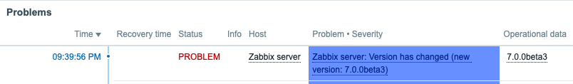
When Zabbix 7.0beta3 got released, I immediately updated my What’s up, home? environment to run it. As usual, the update process was seamless and fast, going through everything in about a minute with my Raspberry Pi 4.
As I updated Zabbix maybe ten minutes ago, these are very real-time impressions of the new version.
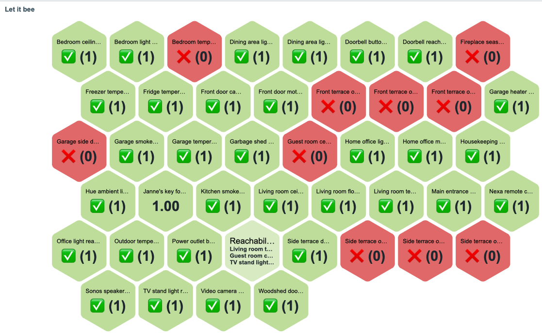
The new honeycomb widget
This new honeycomb widget might be useful! Here’s my first try with it, illustrating the reachability status of my IoT devices.
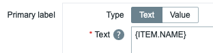
The text shown on widget combs can be modified freely as in the widget advanced config you can put there any Zabbix macro you want.
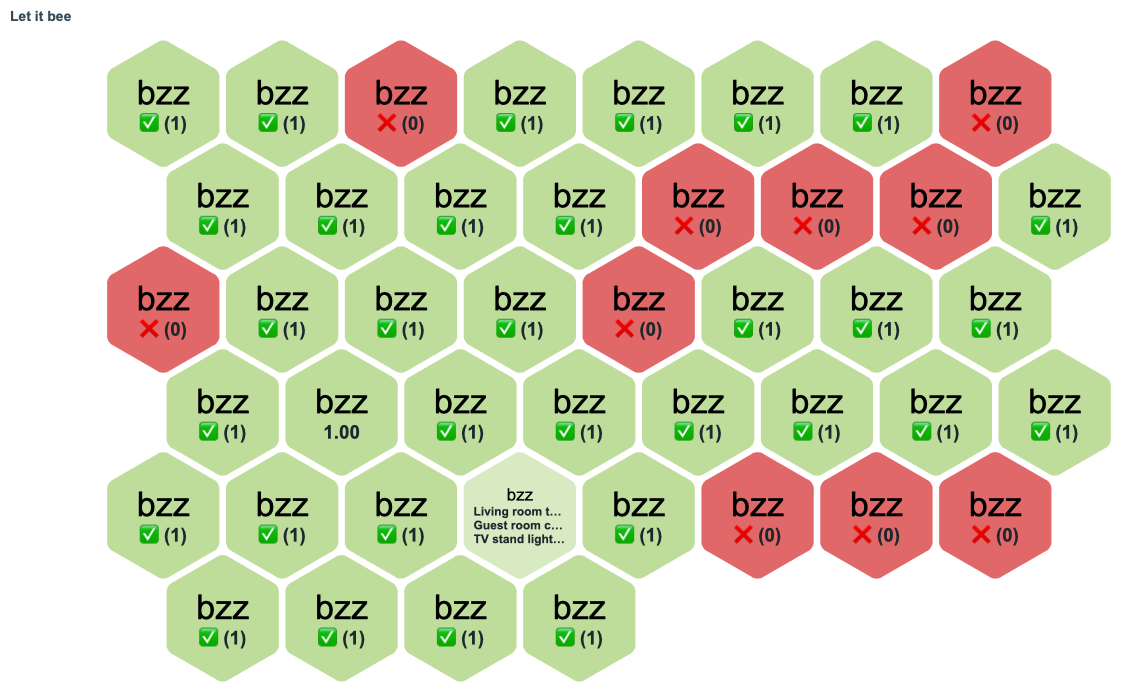
… or if you are such an eternal child that I am, just put there some static text:
The widget supports the new widget communication framework, so whatever item you click there can then be notified by other widgets on the dashboards, to make the experience more interactive.
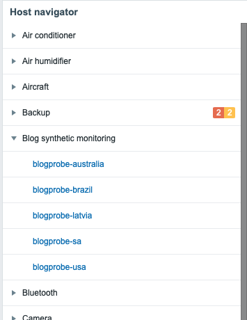
Versatile host navigator widget
There’s another new widget in town, and its name is Host Navigator. With it, you can create a widget that groups your hosts with any criteria by their host groups, or tag values, and it looks like this.
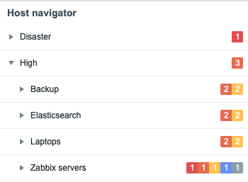
If you then add new widgets or modify the existing ones on your dashboard to receive events from the Host Navigator widget, the changes on other widgets will be reflected in real time. You can also group the items by using multiple rules, for example, first by severity and then by host group, as shown below.
Nice for quick browsing!
Many more improvements
Underneath there’s more going on, but these two were the most visible additions. Other than that, new icons, Zabbix can now execute trigger actions much faster than before (apparently previously there was ~4 seconds lag, now it’s capable of acting in about 100 milliseconds if I read the ticket right), PDF reporting and streaming to external systems are not experimental anymore.
Another solid release marching towards the final version of Zabbix 7.0. In my home environment, these beta versions have been perfectly stable for me.
This post was originally published on the author’s page.
Стойността на човешкия живот и цената, която нашите предци са били готови да платят за неговото спасяване по време на Холокоста отвори врати към знанията и въображението на над 300…
На брега на Коромандел, дето тиквите гърмят, вдън гората, по средата Йонги-Бонги-Бо живя. Стол разбрицан, къс от свещ, кана щърба – тоз младеж имаше едва това. Сред гората той живя, имаше едва това. Туй беше Йонги-Бонги-Бо, туй беше Йонги-Бонги-Бо.
II
Веднъж, когато се помъкна там, дето тиквите гърмят, не щеш ли, взе че се натъкна на куп от камък този път. И ненадейно чу тогаз жена с чаровен, топъл глас с кокошките си да говори. И под носа си промърмори: „Ах, лейди Джингли Джоунс това е! Седи връз камъните, зная! Ах, лейди Джингли Джоунс това е!“ – си рече Йонги-Бонги-Бо, си рече Йонги-Бонги-Бо.
III
„О, Джингли, ти, прекрасна дама! Там, дето тиквите гърмят, дали съпруга ще ми станеш? Тъй уморен ми е духът! Така самотен аз живея на този бряг чакълест, див, самичък веч едва съм жив! Вземи ме ти, аз в теб съм влюбен, животът ми ще стане хубав!“ Тъй рече Йонги-Бонги-Бо, тъй рече Йонги-Бонги-Бо.
IV
„На този бряг във Коромандел скариди и пореч растат, и евтини, и изобилни! Гъмжи от риба този кът! Вземи угарката от свещ, и стола също! – със копнеж той рече. – Щърбавата кана! Като морето любовта ми дълбока е! Не ще те мамя!“ Тъй рече Йонги-Бонги-Бо, тъй рече Йонги-Бонги-Бо.
V
Тогаз кахърно му отвърна, обляна цяла в сълзи, тя: „Ах, жалко, но е невъзможно! Ах, ти ужасно закъсня! Аз с радост бих се съгласила…“ (и тук закърши пръсти, милата) „… но в Англия си имам друг и той ще стане мой съпруг! За жалост, Йонги-Бонги-Бо, за жалост, Йонги-Бонги-Бо!
VI
Той, мистър Джоунс, се казва Хендъл. Кокошки праща ми оттам, от Доркинг, право от пазара. Без него ще е зор голям! Задръж си стола и свещта, и щърба кана аз не ща, но нека дружки сме си още! Щом Хендъл прати ми кокошки, на тебе цели три ще дам! Да знаеш, Йонги-Бонги-Бо, да знаеш, Йонги-Бонги-Бо!
VII
Макар и да си толкоз хилав, но с грамаданска пък глава, и шапката ти все да хвърка – да знаеш, че е затова! Макар и да си тъпоумен, аз исках да намеря думи, за да се изразя по-меко… Та, ще си тръгваш ли полека? Какво да кажа друго нямам, остава да се махнеш само! Това е, Йонги-Бонги-Бо, това е, Йонги-Бонги Бо!“
VIII
По хлъзгавия склон на Мъртъл, там, дето тиквите гърмят, наш Йонги-Бонги-Бо си хвана към тихите морета път. Зад залив кротко си лежеше огромна костенурка. Беше известна с туй, че бързо плава. Какво на него му остава? „Ха, ето кой ще ме спаси! Я ти на гръб ме понеси!“ Тъй рече Йонги-Бонги-Бо, тъй рече Йонги-Бонги-Бо.
IX
Из океана, що бушува и кротва се, и се снишава, със Йонги-Бонги-Бо на гръб чевръсто костенурка плава. Към остров Бошен тя го кара и със движения прастари, печални, плава, накъдето потъва слънцето в морето. „Прощавай, лейди Джингли, сбогом! Без тебе да живея мога!“ – тъй пя си Йонги-Бонги-Бо, тъй пя си Йонги-Бонги-Бо.
Х
А на брега на Коромандел онази дама си остана и тя за Йонги вечно жали там, върху купчината камък. Затуй в нащърбената кана тя сълзи рони. Отзарана и камънака там измива, като със сълзи го облива. И прегъната на две, на кокошките реве тя за Йонги-Бонги-Бо, тя за Йонги-Бонги-Бо.
Едуард Лиър Превод от английски Светлана Комогорова – Комата
Едуард Лиър (1812–1888) е английски поет, писател, художник, илюстратор и музикант, автор на няколко популярни сборника с нонсенс стихотворения, разкази и песни. Роден е в Холоуей, Северен Лондон, и е предпоследното от 21 деца на Ан Кларк Скерет и Джеремая Лиър. Известен е най-вече със своите нонсенс поетични и прозаични творби и особено с лимериците – форма, която той популяризира. За произведенията му е характерна изключителната езикова изобретателност. Като музикант е единственият автор на песни по текстове на Алфред Тенисън, чиято музика самият Тенисън е одобрил. Много свои нонсенс текстове също претворява в песни, включително и „Ухажорът Йонги-Бонги-Бо“. Известен е и с това, че се представя с дългите псевдоними Mr Abebika kratoponoko Prizzikalo Kattefello Ablegorabalus Ableborinto phashyph или Chakonoton the Cozovex Dossi Fossi Sini Tomentilla Coronilla Polentilla Battledore & Shuttlecock Derry down Derry Dumps.
Светлана Комогорова – Комата (р. 1968) е преводачка, поетеса, певица и автор на песни. Носителка на Специалната награда „Кръстан Дянков“ (2010) за превода на „Шантарам“ от Грегъри Дейвид Робъртс; номинирана два пъти за наградата „Евроком“ за превод на фантастика, както и за наградата „Христо Г. Данов“ (2005) за превода на „Лед“ от Владимир Сорокин. Много обича Луис Карол, а най-любимите ѝ произведения са „Алиса в страната на чудесата“ и „Алиса в огледалния свят“. Авторка е на два напълно различни превода на двете книги – единият, съвместен със Силвия Вълкова, е публикуван за първи път през 1996 г. от издателство „Дамян Яков“ и оттогава е преиздаван няколко пъти, а другият – през 2022 г. от издателство „Хеликон“. Изпитва подчертано и невъобразимо влечение към нонсенса в литературата и в изкуството изобщо.
Според Екатерина Йосифова „четящият стихотворение сутрин… добре понася другите часове“ от деня. Убедени, че поезията държи умовете ни будни, а сърцата – отворени, в края на всеки месец ви предлагаме по едно стихотворение. Защото и в най-смутни времена доброто стихотворение е добра новина.
The collective thoughts of the interwebz
Manage Consent
To provide the best experiences, we use technologies like cookies to store and/or access device information. Consenting to these technologies will allow us to process data such as browsing behavior or unique IDs on this site. Not consenting or withdrawing consent, may adversely affect certain features and functions.
Functional
Always active
The technical storage or access is strictly necessary for the legitimate purpose of enabling the use of a specific service explicitly requested by the subscriber or user, or for the sole purpose of carrying out the transmission of a communication over an electronic communications network.
Preferences
The technical storage or access is necessary for the legitimate purpose of storing preferences that are not requested by the subscriber or user.
Statistics
The technical storage or access that is used exclusively for statistical purposes.The technical storage or access that is used exclusively for anonymous statistical purposes. Without a subpoena, voluntary compliance on the part of your Internet Service Provider, or additional records from a third party, information stored or retrieved for this purpose alone cannot usually be used to identify you.
Marketing
The technical storage or access is required to create user profiles to send advertising, or to track the user on a website or across several websites for similar marketing purposes.


 Pradeep Misra is a Principal Analytics Solutions Architect at AWS. He works across Amazon to architect and design modern distributed analytics and AI/ML platform solutions. He is passionate about solving customer challenges using data, analytics, and AI/ML. Outside of work, Pradeep likes exploring new places, trying new cuisines, and playing board games with his family. He also likes doing science experiments with his daughters.
 Deepmala Agarwal works as an AWS Data Specialist Solutions Architect. She is passionate about helping customers build out scalable, distributed, and data-driven solutions on AWS. When not at work, Deepmala likes spending time with family, walking, listening to music, watching movies, and cooking!
 Abhilash Nagilla is a Senior Specialist Solutions Architect at Amazon Web Services (AWS), helping public sector customers on their cloud journey with a focus on AWS analytics services. Outside of work, Abhilash enjoys learning new technologies, watching movies, and visiting new places.


 OpenapiBlogStack
 Deployment time: 97.78s
Outputs:
OpenapiBlogStack.OpenApiGatewayToLambdaSpecRestApiEndpointD1FA5E3A = https://b73nx617gl.execute-api.us-east-1.amazonaws.com/prod/
OpenapiBlogStack.OrderUrl = https://b73nx617gl.execute-api.us-east-1.amazonaws.com/prod/order
Stack ARN:
arn:aws:cloudformation:us-east-1:123456789012:stack/OpenapiBlogStack/01df6970-dc05-11ee-a0eb-0a97cfc33817
Deployment time: 97.78s
Outputs:
OpenapiBlogStack.OpenApiGatewayToLambdaSpecRestApiEndpointD1FA5E3A = https://b73nx617gl.execute-api.us-east-1.amazonaws.com/prod/
OpenapiBlogStack.OrderUrl = https://b73nx617gl.execute-api.us-east-1.amazonaws.com/prod/order
Stack ARN:
arn:aws:cloudformation:us-east-1:123456789012:stack/OpenapiBlogStack/01df6970-dc05-11ee-a0eb-0a97cfc33817