Post Syndicated from The History Guy: History Deserves to Be Remembered original https://www.youtube.com/watch?v=fL6xHsDHSvc
Abraham Galloway, Spy for the Union
Post Syndicated from The History Guy: History Deserves to Be Remembered original https://www.youtube.com/watch?v=HnCfbBY2FN8
The World’s Most Dangerous Year
Post Syndicated from The History Guy: History Deserves to Be Remembered original https://www.youtube.com/watch?v=0_HhjF-Dze4
Black Monday: 250th Mission of the Eight Air Force
Post Syndicated from The History Guy: History Deserves to Be Remembered original https://www.youtube.com/watch?v=jvv70FkLAVE
$50 vs $12,000 Projectors Side by Side || Budget vs Performance Comparisons.
Post Syndicated from The Hook Up original https://www.youtube.com/watch?v=NCfnwnLk8Yo
[$] A tale of two troublesome drivers
Post Syndicated from corbet original https://lwn.net/Articles/969383/
The kernel project merges dozens of drivers with every development cycle,
and almost every one of those drivers is entirely uncontroversial.
Occasionally, though, a driver submission raises wider questions, leading
to lengthy discussion and, perhaps, opposition. That is currently the case
with two separate drivers, both with ties to the networking subsystem. One
of them is hung up on questions of whether (and how) all device
functionality should be made available to user space, while the other has
run into turbulence because it drives a device that is unobtainable outside
of a single company.
What we need to take away from the XZ Backdoor (openSUSE News)
Post Syndicated from corbet original https://lwn.net/Articles/969591/
Dirk Mueller has posted a
lengthy analysis of the XZ backdoor on the openSUSE News site, with a
focus on openSUSE’s response.
Debian, as well as the other affected distributions like openSUSE
are carrying a significant amount of downstream-only patches to
essential open-source projects, like in this case OpenSSH. With
hindsight, that should be another Heartbleed-level learning for the
work of the distributions. These patches built the essential steps
to embed the backdoor, and do not have the scrutiny that they
likely would have received by the respective upstream
maintainers. Whether you trust Linus Law or not, it was not even
given a chance to chime in here. Upstream did not fail on the
users, distributions failed on upstream and their users here.
Security updates for Friday
Post Syndicated from daroc original https://lwn.net/Articles/969590/
Security updates have been issued by Debian (chromium), Fedora (rust, trafficserver, and upx), Mageia (postgresql-jdbc and x11-server, x11-server-xwayland, tigervnc), Red Hat (bind, bind9.16, gnutls, httpd:2.4, squid, unbound, and xorg-x11-server), SUSE (perl-Net-CIDR-Lite), and Ubuntu (apache2, maven-shared-utils, and nss).
Improving authoritative DNS with the official release of Foundation DNS
Post Syndicated from Hannes Gerhart original https://blog.cloudflare.com/foundation-dns-launch
We are very excited to announce the official release of Foundation DNS, with new advanced nameservers, even more resilience, and advanced analytics to meet the complex requirements of our enterprise customers. Foundation DNS is one of Cloudflare’s largest leaps forward in our authoritative DNS offering since its launch in 2010, and we know our customers are interested in an enterprise-ready authoritative DNS service with the highest level of performance, reliability, security, flexibility, and advanced analytics.
Starting today, every new enterprise contract that includes authoritative DNS will have access to the Foundation DNS feature set and existing enterprise customers will have Foundation DNS features made available to them over the course of this year. If you are an existing enterprise customer already using our authoritative DNS services, and you’re interested in getting your hands on Foundation DNS earlier, just reach out to your account team, and they can enable it for you. Let’s get started…
Why is DNS so important?
From an end user perspective, DNS makes the Internet usable. DNS is the phone book of the Internet which translates hostnames like www.cloudflare.com into IP addresses that our browsers, applications, and devices use to connect to services. Without DNS, users would have to remember IP addresses like 108.162.193.147 or 2606:4700:58::adf5:3b93 every time they wanted to visit a website on their mobile device or desktop – imagine having to remember something like that instead of just www.cloudflare.com. DNS is used in every end user application on the Internet, from social media to banking to healthcare portals. People’s usage of the Internet is entirely reliant on DNS.
From a business perspective, DNS is the very first step in reaching websites and connecting to applications. Devices need to know where to connect in order to reach services, authenticate users, and provide the information being requested. Resolving DNS queries quickly can be the difference between a website or application being perceived as responsive or not and can have a real impact on user experience.
When DNS outages occur, the impacts are obvious. Imagine your go-to ecommerce site not loading, just like what happened with the outage Dyn experienced in 2016, which took down multiple popular ecommerce sites among others. Or, if you are part of a company, and customers aren’t able to reach your website to purchase the goods or services you are selling, a DNS outage will literally lose you money. DNS is often taken for granted, but make no mistake, you’ll notice it when it’s not working properly. Thankfully, if you use Cloudflare Authoritative DNS, these are problems you don’t worry about very much.
There is always room for improvement
Cloudflare has been providing authoritative DNS services for over a decade. Our authoritative DNS service hosts millions of domains across many different top level domains (TLDs). We have customers of all sizes, from single domains with just a few records to customers with tens of millions of records spread across multiple domains. Our enterprise customers, rightfully, demand the highest level of performance, reliability, security, and flexibility from our DNS service, along with detailed analytics. While our customers love our authoritative DNS, we recognize there is always room for improvement in some of those categories. To that end, we set off to make some major improvements to our DNS architecture, with new features as well as structural changes. We are proudly calling this improved offering Foundation DNS.
Meet Foundation DNS
As our new enterprise authoritative DNS offering, Foundation DNS was designed to enhance the reliability, security, flexibility, and analytics of our existing authoritative DNS service. Before we dive into all the specifics of Foundation DNS, here is a quick summary of what Foundation DNS brings to our authoritative DNS offering:
- Advanced nameservers bring DNS reliability to the next level.
- New zone-level DNS settings provide more flexible configuration of DNS specific settings.
- Unique DNSSEC keys per account and zone provide additional security and flexibility for DNSSEC.
- GraphQL-based DNS analytics provide even more insights into your DNS queries.
- A new release process ensures enterprise customers have the utmost stability and reliability.
- Simpler DNS pricing with more generous quotas for DNS-only zones and DNS records.
Now, let’s dive deeper into each of these new Foundation DNS features:
Advanced nameservers
With Foundation DNS, we’re introducing advanced nameservers with a specific focus on enhancing reliability for your enterprise. You might be familiar with our standard authoritative nameservers which come as a pair per zone and use names within the cloudflare.com domain. Here’s an example:
$ dig mycoolwebpage.xyz ns +noall +answer
mycoolwebpage.xyz.	86400	IN	NS	kelly.ns.cloudflare.com.
mycoolwebpage.xyz.	86400	IN	NS	christian.ns.cloudflare.com.
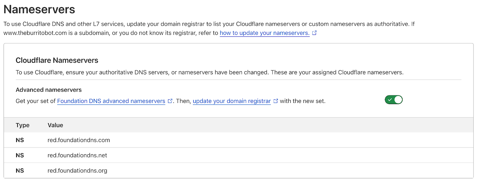
Now, let’s look at the same zone using Foundation DNS advanced nameservers:
$ dig mycoolwebpage.xyz ns +noall +answer
mycoolwebpage.xyz.	86400	IN	NS	blue.foundationdns.com.
mycoolwebpage.xyz.	86400	IN	NS	blue.foundationdns.net.
mycoolwebpage.xyz.	86400	IN	NS	blue.foundationdns.org.
Advanced nameservers improve reliability in a few different ways. The first improvement comes from the Foundation DNS authoritative servers being spread across multiple TLDs. This provides protection from larger scale DNS outages and DDoS attacks that could potentially affect DNS infrastructure further up the tree, including TLD name servers. Foundation DNS authoritative nameservers are now located across multiple branches of the global DNS tree structure, further insulating our customers from these potential outages and attacks.
You might also have noticed that there is an additional nameserver listed with Foundation DNS. While this is an improvement, it’s not for the reason you might think it is. If we resolve each one of these nameservers to their respective IP addresses, we can make this a little easier to understand. Let’s do that here starting with our standard nameservers:
$ dig kelly.ns.cloudflare.com. +noall +answer
kelly.ns.cloudflare.com. 86353  IN      A       108.162.194.91
kelly.ns.cloudflare.com. 86353  IN      A       162.159.38.91
kelly.ns.cloudflare.com. 86353  IN      A       172.64.34.91

$ dig christian.ns.cloudflare.com. +noall +answer
christian.ns.cloudflare.com. 86353 IN   A       108.162.195.247
christian.ns.cloudflare.com. 86353 IN   A       162.159.44.247
christian.ns.cloudflare.com. 86353 IN   A       172.64.35.247
There are six total IP addresses for the two nameservers. As it turns out, this is all DNS resolvers actually care about when querying authoritative nameservers. DNS resolvers usually don’t track the actual domain names of authoritative servers; they simply maintain an unordered list of IP addresses that they can use to resolve queries for a given domain. So with our standard authoritative nameservers, we give resolvers six IP addresses to use to resolve DNS queries. Now, let’s look at the IP addresses for our Foundation DNS advanced nameservers:
$ dig blue.foundationdns.com. +noall +answer
blue.foundationdns.com. 300     IN      A       108.162.198.1
blue.foundationdns.com. 300     IN      A       162.159.60.1
blue.foundationdns.com. 300     IN      A       172.64.40.1

$ dig blue.foundationdns.net. +noall +answer
blue.foundationdns.net. 300     IN      A       108.162.198.1
blue.foundationdns.net. 300     IN      A       162.159.60.1
blue.foundationdns.net. 300     IN      A       172.64.40.1

$ dig blue.foundationdns.org. +noall +answer
blue.foundationdns.org. 300     IN      A       108.162.198.1
blue.foundationdns.org. 300     IN      A       162.159.60.1
blue.foundationdns.org. 300     IN      A       172.64.40.1
Would you look at that! Foundation DNS provides the same IP addresses for each of the authoritative nameservers that we provide to a zone. So in this case, we have only provided three IP addresses for resolvers to use to resolve DNS queries. And you might be wondering,“isn’t six better than three? Isn’t this a downgrade?” It turns out more isn’t always better. Let’s talk about why.
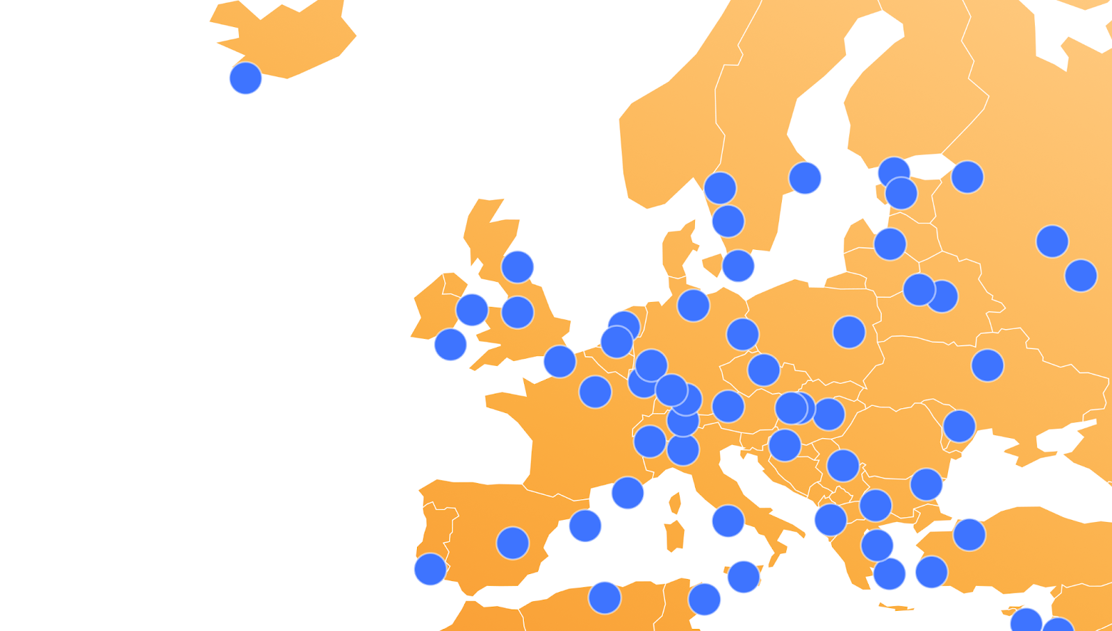
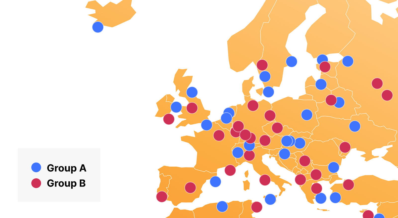
You are probably aware of Cloudflare’s use of Anycast and, as you might assume, our DNS services leverage Anycast to ensure that our authoritative DNS servers are available globally and as close as possible to users and resolvers across the Internet. Our standard nameservers are all advertised out of every Cloudflare data center by a single Anycast group. If we zoom in on Europe, you can see that in a standard nameserver deployment, both nameservers are advertised from every data center.
We can take those six IP addresses from our standard nameservers above and perform a lookup for their “hostname.bind” TXT record which will show us the airport code or physical location of the closest data center where our DNS queries are being resolved from. This output helps explain the reason why more isn’t always better.
$ dig @108.162.194.91 ch txt hostname.bind +short
"LHR"

$ dig @162.159.38.91 ch txt hostname.bind +short
"LHR"

$ dig @172.64.34.91 ch txt hostname.bind +short
"LHR"

$ dig @108.162.195.247 ch txt hostname.bind +short
"LHR"

$ dig @162.159.44.247 ch txt hostname.bind +short
"LHR"

$ dig @172.64.35.247 ch txt hostname.bind +short
"LHR"
As you can see, when queried from near London, all six of those IP addresses route to the same London (LHR) data center. Meaning that when a resolver in London is resolving DNS queries for a domain using Cloudflare’s standard authoritative DNS, no matter which nameserver IP address is being queried, they are always connecting to the same physical location.
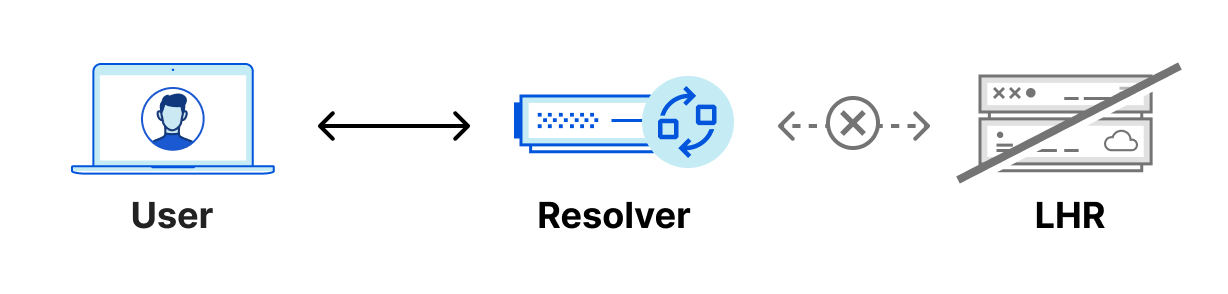
You might be asking, “So what? What does that mean to me?” Let’s look at an example. If you wanted to resolve a domain using Cloudflare standard nameservers from London, and I am using a public resolver that is also located in London, the resolver will always connect to the Cloudflare LHR data center regardless of which nameserver it’s trying to reach. It doesn’t have any other option, because of Anycast.

Because of Anycast, should the LHR data center go offline completely, all the traffic intended for LHR would be routed to other nearby data centers and resolvers would continue to function normally. However, in the unlikely scenario where the LHR data center was online, but our DNS services aren’t able to respond to DNS queries, the resolver would have no way to resolve these DNS queries since they can’t reach out to any other data center. We could have 100 IP addresses, and it would not help us in this scenario. Eventually, cached responses will expire, and the domain will eventually stop being resolved.
Foundation DNS advanced nameservers are changing the way we use Anycast by leveraging two Anycast groups, which breaks the previous paradigm of every authoritative nameserver IP being advertised from every data center. Using two Anycast groups means that Foundation DNS authoritative nameservers actually have different physical locations from one another, rather than all being advertised from each data center. Here is how that same region would look using two Anycast groups:
Let’s go back and finish our comparison of six authoritative IP addresses for standard authoritative DNS vs three IP addresses for Foundation DNS now that it’s understood that Foundation DNS is using two Anycast groups for advertising nameservers. Let’s see where Foundation DNS servers are being advertised from for our example:
$ dig @108.162.198.1 ch txt hostname.bind +short
"LHR"

$ dig @162.159.60.1 ch txt hostname.bind +short
"LHR"

$ dig @172.64.40.1 ch txt hostname.bind +short
"MAN"
Look at that! One of our three nameserver IP addresses is being advertised out of a different data center, Manchester (MAN), making Foundation DNS more reliable and resilient for the previously mentioned outage scenario. It’s worth mentioning that in some cities, Cloudflare operates out of multiple data centers which will result in all three queries returning the same airport code. While we guarantee that at least one of those IP addresses is being advertised out of a different data center, we understand some customers may want to test for themselves. In those cases, an additional query can show that IP addresses are being advertised out of different data centers.
$ dig @108.162.198.1 +nsid | grep NSID:
; NSID: 39 34 6d 33 39 ("94m39")
In the “94m30” returned in the response, the number before the “m” represents the data center that answered the query. As long as that number is different in one of the three responses, you know that one of your Foundation DNS authoritative nameservers is being advertised out of a different physical location.
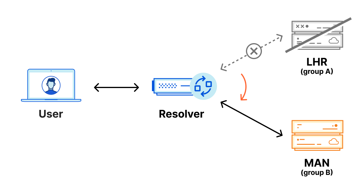
With Foundation DNS leveraging two Anycast groups, the previous outage scenario is handled seamlessly. DNS resolvers monitor requests to all the authoritative nameservers returned for a given domain, but primarily use the nameserver that is providing the fastest responses.
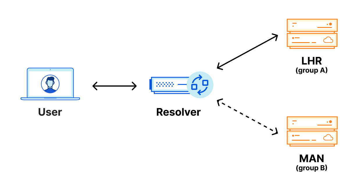
With this configuration, DNS resolvers are able to send requests to two different Cloudflare data centers, so, should a failure happen at one physical location, queries are then automatically sent to the second data center where they can be properly resolved.
Foundation DNS advanced nameservers are a big step forward in reliability for our enterprise customers. We welcome our enterprise customers to enable advanced nameservers for existing zones today. Migrating to Foundation DNS won’t involve any downtime either because even after Foundation DNS advanced nameservers are enabled for a zone, the previous standard authoritative DNS nameservers will continue to function and respond to queries for the zone. Customers don’t need to plan for a cutover or other service-impacting event to migrate to Foundation DNS advanced nameservers.
New zone-level DNS settings
Historically, we have received regular requests from our enterprise customers to adjust specific DNS settings that were not exposed via our API or dashboard, such as enabling secondary DNS overrides. When customers wanted these settings adjusted, they had to reach out to their account teams, who would change the configurations. With Foundation DNS, we are exposing the most commonly requested settings via the API and dashboard to give our customers increased flexibility with their Cloudflare authoritative DNS solution.
Enterprise customers can now configure the following DNS settings on their zones:
| Setting | Zone Type | Description |
|---|---|---|
| Foundation DNS advanced nameservers | Primary and secondary zones | Allows you to enable advanced nameservers on your zone. |
| Secondary DNS override | Secondary zones | Allows you to enable Secondary DNS Override on your zone in order to proxy HTTP/S traffic through Cloudflare. |
| Multi-provider DNS | Primary and secondary zones | Allows you to have multiple authoritative DNS providers while using Cloudflare as a primary nameserver. |
Unique DNSSEC keys per account and zone
DNSSEC, which stands for Domain Name System Security Extensions, adds security to a domain or zone by providing a way to check that the response you receive for a DNS query is authentic and hasn’t been modified. DNSSEC prevents DNS cache poisoning (DNS spoofing) which helps ensure that DNS resolvers are responding to DNS queries with the correct IP addresses.
Since we launched Universal DNSSEC in 2015, we’ve made quite a few improvements, like adding support for pre-signed DNSSEC for secondary zones and multi-signer DNSSEC. By default, Cloudflare signs DNS records on the fly (live signing) as we respond to DNS queries. This allows Cloudflare to host a DNSSEC-secured domain while dynamically allocating IP addresses for the proxied origins. It also enables certain load balancing use cases since the IP addresses served in the DNS response in these cases change based on steering.
Cloudflare uses the Elliptic Curve algorithm ECDSA P-256, which is stronger than most RSA keys used today. It uses less CPU to generate signatures, making them more efficient to generate on the fly. Usually two keys are used as part of DNSSEC, the Zone Signing Key (ZSK) and the Key Signing Key (KSK). At the simplest level, the ZSK is used for signing the DNS records that are served in response to queries and the KSK is used to sign the DNSKEYs, including the ZSK to ensure its authenticity.
Today, Cloudflare uses a shared ZSK and KSK globally for all DNSSEC signing, and since we use such a strong cryptographic algorithm, we know how secure this key set is and as such, do not believe there is a need to regularly rotate the ZSK or KSK – at least for security reasons. There are customers, however, that have policies that require the rotation of these keys at certain intervals. Because of this, we’ve added the ability for our new Foundation DNS advanced nameservers to rotate both their ZSK and KSK as needed per account or per zone. This will first be available via the API and subsequently through the Cloudflare dashboard. So now, customers with strict policy requirements around their DNSSEC key rotation can meet those requirements with Cloudflare Foundation DNS.
GraphQL-based DNS analytics
For those who are not familiar with it, GraphQL is a query language for APIs and a runtime for executing those queries. It allows clients to request exactly what they need, no more, no less, enabling them to aggregate data from multiple sources through a single API call, and supports real-time updates through subscriptions.
As you might know, Cloudflare has had a GraphQL API for a while now, but as part of Foundation DNS we are adding a new DNS dataset to that API that is only available with our new Foundation DNS advanced nameservers.
The new DNS dataset in our GraphQL API can be used to fetch information about the DNS queries a zone has received. This faster and more powerful alternative to our current DNS Analytics API allows you to query data from large time periods quickly and efficiently without running into limits or timeouts. The GraphQL API is more flexible with regard to which queries it accepts, and exposes more information than the DNS Analytics API.
For example, you can run this query to fetch the mean and 90th percentile processing time of your queries, grouped by source IP address, in 15 minute buckets. A query like this would be useful to see which IPs are querying your records most often for a given time range:
{
  "query": "{
    viewer {
      zones(filter: { zoneTag: $zoneTag }) {
        dnsAnalyticsAdaptiveGroups(
          filter: $filter
          limit: 10
          orderBy: [datetime_ASC]
        ) {
          avg {
            processingTimeUs
          }
          quantiles {
            processingTimeUsP90
          }
          dimensions {
            datetimeFifteenMinutes
            sourceIP
          }
        }
      }
    }
  }",
  "variables": {
    "zoneTag": "<zone-tag>",
    "filter": {
      "datetime_geq": "2024-05-01T00:00:00Z",
      "datetime_leq": "2024-06-01T00:00:00Z"
    }
  }
}
Previously, a query like this wouldn’t have been possible for several reasons. The first is that we have added new fields like sourceIP, which allows us to filter data based on which client IP addresses (usually resolvers) are making DNS queries. The second is that the GraphQL API query is able to process and return data from much larger time ranges. A DNS zone with sufficiently large amounts of queries was previously only able to query across a few days of traffic, while the new GraphQL API can provide data for a period of up to 31 days. We are planning further enhancements to that range, as well as how far back historical data can be stored and queried.
The GraphQL API also allows us to add a new DNS analytics section to the Cloudflare dashboard. Customers will be able to track the most queried records, see which data centers are answering those queries, see how many queries are being made, and much more.
The new DNS dataset in our GraphQL API and the new DNS analytics page work together to help our DNS customers to monitor, analyze, and troubleshoot their Foundation DNS deployments.
New release process
Cloudflare’s Authoritative DNS product receives software updates roughly once a week. Cloudflare has a sophisticated release process that helps prevent regressions from affecting production traffic. While uncommon, it’s possible to have issues only surface once the new release is subject to the volume and uniqueness of production traffic.
Because our enterprise customers desire stability even more than new features, new releases will be subject to a two-week soak time with our standard nameservers before our Foundation DNS advanced nameservers are upgraded. After two weeks with no issues, the Foundation DNS advanced nameservers will be upgraded as well.
Zones using Foundation DNS advanced nameservers will see increased reliability as they are better protected against regressions in new software releases.
Simpler DNS pricing
Historically, Cloudflare has charged for Authoritative DNS based on monthly DNS queries and the number of domains in the account. Our enterprise DNS customers are often interested in DNS-only zones, which are DNS zones hosted in Cloudflare that do not use our reverse proxy (layer 7) services such as our CDN, WAF, or Bot Management. With Foundation DNS, we’re making pricing simpler for the vast majority of those customers by including 10,000 DNS only domains by default. This change means most customers will only pay for the number of DNS queries they consume.
We’re also including 1 million DNS records across all domains in an account. But that doesn’t mean we can’t support more. In fact, the biggest single zone on our platform has over 3.9 million records, while our largest DNS account is just shy of 30 million DNS records spread across multiple zones. With Cloudflare DNS, there is no trouble handling even the largest deployments.
There is more to come
We are just getting started. In the future, we will add more exclusive features to Foundation DNS. One example is a highly requested feature: per-record scoped API tokens and user permissions. This will allow you to configure permissions on an even more granular level. For example, you could specify that a particular member of your account is only allowed to create and manage records of the type TXT and MX, so they don’t accidentally delete or edit address records impacting web traffic to your domain. Another example would be to specify permissions based on subdomain to further restrict the scope of specific users.
If you’re an existing enterprise customer and want to use Foundation DNS, get in touch with your account team to provision Foundation DNS on your account.
How we ensure Cloudflare customers aren’t affected by Let’s Encrypt’s certificate chain change
Post Syndicated from Dina Kozlov original https://blog.cloudflare.com/shortening-lets-encrypt-change-of-trust-no-impact-to-cloudflare-customers

Let’s Encrypt, a publicly trusted certificate authority (CA) that Cloudflare uses to issue TLS certificates, has been relying on two distinct certificate chains. One is cross-signed with IdenTrust, a globally trusted CA that has been around since 2000, and the other is Let’s Encrypt’s own root CA, ISRG Root X1. Since Let’s Encrypt launched, ISRG Root X1 has been steadily gaining its own device compatibility.
On September 30, 2024, Let’s Encrypt’s certificate chain cross-signed with IdenTrust will expire. After the cross-sign expires, servers will no longer be able to serve certificates signed by the cross-signed chain. Instead, all Let’s Encrypt certificates will use the ISRG Root X1 CA.
Most devices and browser versions released after 2016 will not experience any issues as a result of the change since the ISRG Root X1 will already be installed in those clients’ trust stores. That’s because these modern browsers and operating systems were built to be agile and flexible, with upgradeable trust stores that can be updated to include new certificate authorities.
The change in the certificate chain will impact legacy devices and systems, such as devices running Android version 7.1.1 (released in 2016) or older, as those exclusively rely on the cross-signed chain and lack the ISRG X1 root in their trust store. These clients will encounter TLS errors or warnings when accessing domains secured by a Let’s Encrypt certificate. We took a look at the data ourselves and found that, of all Android requests, 2.96% of them come from devices that will be affected by the change. That’s a substantial portion of traffic that will lose access to the Internet. We’re committed to keeping those users online and will modify our certificate pipeline so that we can continue to serve users on older devices without requiring any manual modifications from our customers.
A better Internet, for everyone
In the past, we invested in efforts like “No Browsers Left Behind” to help ensure that we could continue to support clients as SHA-1 based algorithms were being deprecated. Now, we’re applying the same approach for the upcoming Let’s Encrypt change.
We have made the decision to remove Let’s Encrypt as a certificate authority from all flows where Cloudflare dictates the CA, impacting Universal SSL customers and those using SSL for SaaS with the “default CA” choice.
Starting in June 2024, one certificate lifecycle (90 days) before the cross-sign chain expires, we’ll begin migrating Let’s Encrypt certificates that are up for renewal to use a different CA, one that ensures compatibility with older devices affected by the change. That means that going forward, customers will only receive Let’s Encrypt certificates if they explicitly request Let’s Encrypt as the CA.
The change that Let’s Encrypt is making is a necessary one. For us to move forward in supporting new standards and protocols, we need to make the Public Key Infrastructure (PKI) ecosystem more agile. By retiring the cross-signed chain, Let’s Encrypt is pushing devices, browsers, and clients to support adaptable trust stores.
However, we’ve observed changes like this in the past and while they push the adoption of new standards, they disproportionately impact users in economically disadvantaged regions, where access to new technology is limited.
Our mission is to help build a better Internet and that means supporting users worldwide. We previously published a blog post about the Let’s Encrypt change, asking customers to switch their certificate authority if they expected any impact. However, determining the impact of the change is challenging. Error rates due to trust store incompatibility are primarily logged on clients, reducing the visibility that domain owners have. In addition, while there might be no requests incoming from incompatible devices today, it doesn’t guarantee uninterrupted access for a user tomorrow.
Cloudflare’s certificate pipeline has evolved over the years to be resilient and flexible, allowing us to seamlessly adapt to changes like this without any negative impact to our customers.
How Cloudflare has built a robust TLS certificate pipeline
Today, Cloudflare manages tens of millions of certificates on behalf of customers. For us, a successful pipeline means:
- Customers can always obtain a TLS certificate for their domain
- CA related issues have zero impact on our customer’s ability to obtain a certificate
- The best security practices and modern standards are utilized
- Optimizing for future scale
- Supporting a wide range of clients and devices
Every year, we introduce new optimizations into our certificate pipeline to maintain the highest level of service. Here’s how we do it…
Ensuring customers can always obtain a TLS certificate for their domain
Since the launch of Universal SSL in 2014, Cloudflare has been responsible for issuing and serving a TLS certificate for every domain that’s protected by our network. That might seem trivial, but there are a few steps that have to successfully execute in order for a domain to receive a certificate:
- Domain owners need to complete Domain Control Validation for every certificate issuance and renewal.
- The certificate authority needs to verify the Domain Control Validation tokens to issue the certificate.
- CAA records, which dictate which CAs can be used for a domain, need to be checked to ensure only authorized parties can issue the certificate.
- The certificate authority must be available to issue the certificate.
Each of these steps requires coordination across a number of parties — domain owners, CDNs, and certificate authorities. At Cloudflare, we like to be in control when it comes to the success of our platform. That’s why we make it our job to ensure each of these steps can be successfully completed.
We ensure that every certificate issuance and renewal requires minimal effort from our customers. To get a certificate, a domain owner has to complete Domain Control Validation (DCV) to prove that it does in fact own the domain. Once the certificate request is initiated, the CA will return DCV tokens which the domain owner will need to place in a DNS record or an HTTP token. If you’re using Cloudflare as your DNS provider, Cloudflare completes DCV on your behalf by automatically placing the TXT token returned from the CA into your DNS records. Alternatively, if you use an external DNS provider, we offer the option to Delegate DCV to Cloudflare for automatic renewals without any customer intervention.
Once DCV tokens are placed, Certificate Authorities (CAs) verify them. CAs conduct this verification from multiple vantage points to prevent spoofing attempts. However, since these checks are done from multiple countries and ASNs (Autonomous Systems), they may trigger a Cloudflare WAF rule which can cause the DCV check to get blocked. We made sure to update our WAF and security engine to recognize that these requests are coming from a CA to ensure they’re never blocked so DCV can be successfully completed.
Some customers have CA preferences, due to internal requirements or compliance regulations. To prevent an unauthorized CA from issuing a certificate for a domain, the domain owner can create a Certification Authority Authorization (CAA) DNS record, specifying which CAs are allowed to issue a certificate for that domain. To ensure that customers can always obtain a certificate, we check the CAA records before requesting a certificate to know which CAs we should use. If the CAA records block all of the CAs that are available in Cloudflare’s pipeline and the customer has not uploaded a certificate from the CA of their choice, then we add CAA records on our customers’ behalf to ensure that they can get a certificate issued. Where we can, we optimize for preference. Otherwise, it’s our job to prevent an outage by ensuring that there’s always a TLS certificate available for the domain, even if it does not come from a preferred CA.
Today, Cloudflare is not a publicly trusted certificate authority, so we rely on the CAs that we use to be highly available. But, 100% uptime is an unrealistic expectation. Instead, our pipeline needs to be prepared in case our CAs become unavailable.
Ensuring that CA-related issues have zero impact on our customer’s ability to obtain a certificate
At Cloudflare, we like to think ahead, which means preventing incidents before they happen. It’s not uncommon for CAs to become unavailable — sometimes this happens because of an outage, but more commonly, CAs have maintenance periods every so often where they become unavailable for some period of time.
It’s our job to ensure CA redundancy, which is why we always have multiple CAs ready to issue a certificate, ensuring high availability at all times. If you’ve noticed different CAs issuing your Universal SSL certificates, that’s intentional. We evenly distribute the load across our CAs to avoid any single point of failure. Plus, we keep a close eye on latency and error rates to detect any issues and automatically switch to a different CA that’s available and performant. You may not know this, but one of our CAs has around 4 scheduled maintenance periods every month. When this happens, our automated systems kick in seamlessly, keeping everything running smoothly. This works so well that our internal teams don’t get paged anymore because everything just works.
Adopting best security practices and modern standards
Security has always been, and will continue to be, Cloudflare’s top priority, and so maintaining the highest security standards to safeguard our customer’s data and private keys is crucial.
Over the past decade, the CA/Browser Forum has advocated for reducing certificate lifetimes from 5 years to 90 days as the industry norm. This shift helps minimize the risk of a key compromise. When certificates are renewed every 90 days, their private keys remain valid for only that period, reducing the window of time that a bad actor can make use of the compromised material.
We fully embrace this change and have made 90 days the default certificate validity period. This enhances our security posture by ensuring regular key rotations, and has pushed us to develop tools like DCV Delegation that promote automation around frequent certificate renewals, without the added overhead. It’s what enables us to offer certificates with validity periods as low as two weeks, for customers that want to rotate their private keys at a high frequency without any concern that it will lead to certificate renewal failures.
Cloudflare has always been at the forefront of new protocols and standards. It’s no secret that when we support a new protocol, adoption skyrockets. This month, we will be adding ECDSA support for certificates issued from Google Trust Services. With ECDSA, you get the same level of security as RSA but with smaller keys. Smaller keys mean smaller certificates and less data passed around to establish a TLS connection, which results in quicker connections and faster loading times.
Optimizing for future scale
Today, Cloudflare issues almost 1 million certificates per day. With the recent shift towards shorter certificate lifetimes, we continue to improve our pipeline to be more robust. But even if our pipeline can handle the significant load, we still need to rely on our CAs to be able to scale with us. With every CA that we integrate, we instantly become one of their biggest consumers. We hold our CAs to high standards and push them to improve their infrastructure to scale. This doesn’t just benefit Cloudflare’s customers, but it helps the Internet by requiring CAs to handle higher volumes of issuance.
And now, with Let’s Encrypt shortening their chain of trust, we’re going to add an additional improvement to our pipeline — one that will ensure the best device compatibility for all.
Supporting all clients — legacy and modern
The upcoming Let’s Encrypt change will prevent legacy devices from making requests to domains or applications that are protected by a Let’s Encrypt certificate. We don’t want to cut off Internet access from any part of the world, which means that we’re going to continue to provide the best device compatibility to our customers, despite the change.
Because of all the recent enhancements, we are able to reduce our reliance on Let’s Encrypt without impacting the reliability or quality of service of our certificate pipeline. One certificate lifecycle (90 days) before the change, we are going to start shifting certificates to use a different CA, one that’s compatible with the devices that will be impacted. By doing this, we’ll mitigate any impact without any action required from our customers. The only customers that will continue to use Let’s Encrypt are ones that have specifically chosen Let’s Encrypt as the CA.
What to expect of the upcoming Let’s Encrypt change
Let’s Encrypt’s cross-signed chain will expire on September 30th, 2024. Although Let’s Encrypt plans to stop issuing certificates from this chain on June 6th, 2024, Cloudflare will continue to serve the cross-signed chain for all Let’s Encrypt certificates until September 9th, 2024.
90 days or one certificate lifecycle before the change, we are going to start shifting Let’s Encrypt certificates to use a different certificate authority. We’ll make this change for all products where Cloudflare is responsible for the CA selection, meaning this will be automatically done for customers using Universal SSL and SSL for SaaS with the “default CA” choice.
Any customers that have specifically chosen Let’s Encrypt as their CA will receive an email notification with a list of their Let’s Encrypt certificates and information on whether or not we’re seeing requests on those hostnames coming from legacy devices.
After September 9th, 2024, Cloudflare will serve all Let’s Encrypt certificates using the ISRG Root X1 chain. Here is what you should expect based on the certificate product that you’re using:
Universal SSL
With Universal SSL, Cloudflare chooses the CA that is used for the domain’s certificate. This gives us the power to choose the best certificate for our customers. If you are using Universal SSL, there are no changes for you to make to prepare for this change. Cloudflare will automatically shift your certificate to use a more compatible CA.
Advanced Certificates
With Advanced Certificate Manager, customers specifically choose which CA they want to use. If Let’s Encrypt was specifically chosen as the CA for a certificate, we will respect the choice, because customers may have specifically chosen this CA due to internal requirements, or because they have implemented certificate pinning, which we highly discourage.
If we see that a domain using an Advanced certificate issued from Let’s Encrypt will be impacted by the change, then we will send out email notifications to inform those customers which certificates are using Let’s Encrypt as their CA and whether or not those domains are receiving requests from clients that will be impacted by the change. Customers will be responsible for changing the CA to another provider, if they chose to do so.
SSL for SaaS
With SSL for SaaS, customers have two options: using a default CA, meaning Cloudflare will choose the issuing authority, or specifying which CA to use.
If you’re leaving the CA choice up to Cloudflare, then we will automatically use a CA with higher device compatibility.
If you’re specifying a certain CA for your custom hostnames, then we will respect that choice. We will send an email out to SaaS providers and platforms to inform them which custom hostnames are receiving requests from legacy devices. Customers will be responsible for changing the CA to another provider, if they chose to do so.
Custom Certificates
If you directly integrate with Let’s Encrypt and use Custom Certificates to upload your Let’s Encrypt certs to Cloudflare then your certificates will be bundled with the cross-signed chain, as long as you choose the bundle method “compatible” or “modern” and upload those certificates before September 9th, 2024. After September 9th, we will bundle all Let’s Encrypt certificates with the ISRG Root X1 chain. With the “user-defined” bundle method, we always serve the chain that’s uploaded to Cloudflare. If you upload Let’s Encrypt certificates using this method, you will need to ensure that certificates uploaded after September 30th, 2024, the date of the CA expiration, contain the right certificate chain.
In addition, if you control the clients that are connecting to your application, we recommend updating the trust store to include the ISRG Root X1. If you use certificate pinning, remove or update your pin. In general, we discourage all customers from pinning their certificates, as this usually leads to issues during certificate renewals or CA changes.
Conclusion
Internet standards will continue to evolve and improve. As we support and embrace those changes, we also need to recognize that it’s our responsibility to keep users online and to maintain Internet access in the parts of the world where new technology is not readily available. By using Cloudflare, you always have the option to choose the setup that’s best for your application.
For additional information regarding the change, please refer to our developer documentation.
CVE-2024-3400: Critical Command Injection Vulnerability in Palo Alto Networks Firewalls
Post Syndicated from Caitlin Condon original https://blog.rapid7.com/2024/04/12/etr-cve-2024-3400-critical-command-injection-vulnerability-in-palo-alto-networks-firewalls-2/
On Friday, April 12, Palo Alto Networks published an advisory on CVE-2024-3400, a CVSS 10 vulnerability in several versions of PAN-OS, the operating system that runs on the company’s firewalls. According to the vendor advisory, if conditions for exploitability are met, the vulnerability may enable an unauthenticated attacker to execute arbitrary code with root privileges on the firewall. The vulnerability is currently unpatched. Patches are expected to be available by Sunday, April 14, 2024.
Note: Palo Alto Networks customers are only vulnerable if they are using PAN-OS 10.2, PAN-OS 11.0, and/or PAN-OS 11.1 firewalls with the configurations for both GlobalProtect gateway and device telemetry enabled.
Palo Alto Networks’ advisory indicates that CVE-2024-3400 has been exploited in the wild in “a limited number of attacks.” The company has given the vulnerability their highest urgency rating.
Mitigation guidance
CVE-2024-3400 is unpatched as of Friday, April 12 and affects the following versions of PAN-OS when GlobalProtect gateway and device telemetry are enabled:
- PAN-OS 11.1 (before 11.1.2-h3)
- PAN-OS 11.0 (before 11.0.4-h1)
- PAN-OS 10.2 (before 10.2.9-h1)
Palo Alto Networks’ Cloud NGFW and Prisma Access solutions are not affected; nor are earlier versions of PAN-OS (10.1, 10.0, 9.1, and 9.0). For additional information and the latest remediation guidance, please see Palo Alto Networks’ advisory.
The company has indicated that hotfix releases of PAN-OS 10.2.9-h1, PAN-OS 11.0.4-h1, and PAN-OS 11.1.2-h3 will be released by April 14, along with hotfixes for “all later PAN-OS versions.”
Rapid7 recommends applying one of the below vendor-provided mitigations immediately:
- Customers with a Threat Prevention subscription can block attacks for this vulnerability by enabling Threat ID 95187 (introduced in Applications and Threats content version 8833-8682). In addition to enabling Threat ID 95187, customers should ensure vulnerability protection has been applied to their GlobalProtect interface to prevent exploitation of this issue on their device. More information here.
- Those unable to apply the Threat Prevention mitigation can mitigate by temporarily disabling device telemetry until the device is upgraded to a fixed PAN-OS version. Once upgraded, device telemetry should be re-enabled on the device.
Rapid7 customers
Authenticated vulnerability checks are expected to be available to InsightVM and Nexpose customers in today’s (Friday, April 12) content release.
Per the vendor advisory, organizations that are running vulnerable firewalls and are concerned about potential exploitation in their environments can open a support case with Palo Alto Networks to determine if their device logs match known indicators of compromise (IoCs) for this vulnerability.
J J Webb: Lawman to Outlaw
Post Syndicated from The History Guy: History Deserves to Be Remembered original https://www.youtube.com/watch?v=Il8hhqKY3d4
Кал, чистки и избори
Post Syndicated from Емилия Милчева original https://www.toest.bg/kal-chistki-i-izbori/

Парламентът не работи, макар депутатите да ходят на работа, служебният кабинет започна с уволненията, а прокуратурата действа като повредена канализация. В ход е институционализиран погром над ПП–ДБ, комбиниран с удари по репутацията им, които се сипят от всички страни.
След изборите на 9 юни, в зависимост от резултатите, политиците може да изпробват нова формула на властта – експертен кабинет с широка подкрепа, за каквато намекна лидерът на ГЕРБ Бойко Борисов, или коалиция от няколко политически сили.
Два месеца преди изборите, с уговорка за висока степен на неясност, излязоха първи социологически данни, за които „Галъп“ са интервюирали 805 души. ГЕРБ–СДС биха взели 27,4% от гласовете, ПП–ДБ – 17,9%, ДПС – 15,2%, „Възраждане“ – 14,9%, БСП – 10,5%, ИТН – 5,2%.
Второ проучване – на „Маркет Линкс“, сред 1046 души дава сходни резултати. 25,5% от решилите да гласуват ще го направят за ГЕРБ–СДС, 17,1% – за ПП–ДБ. Следват ДПС с резултат от 11,8% и „Възраждане“ – с 10,3%, БСП събира 8,7%, а ИТН остава под 4-процентовия праг.
49-тият парламент произвежда комисии
В остатъка от съществуването си 49-тото НС също завъртя машинката за компрометиращи твърдения. Създадената наскоро временна парламентарна комисия „за разследване на корупционните практики в Агенция „Митници“ и евентуална роля на бившия финансов министър Асен Василев в тях“ с председател Тошко Йорданов (ИТН) вече има списък с лица, които да изслуша. Огънят, разпален от скандала с ареста на шефката на Агенцията – Петя Банкова, трябва да се поддържа с бензина на нови публични разкрития от прокуратурата, ДАНС, Антикорупционната комисия, бившето ръководство на митниците и т.н. Целта е да не замръкне образът на подскачащия сред пачки европудел.
В същото време друга временна парламентарна комисия приключи с работата си по проучването на 13-годишната сделка на България с турската компания „Боташ“, сключена от служебното правителство на президента. (Споразумението между „Булгаргаз“ и „Боташ“ бе подписано в началото на 2023 г., когато на власт бе първият служебен кабинет на Гълъб Донев.) Решението е да изпрати договора на прокуратурата и ДАНС, но последната дума за това имат депутатите в пленарната зала.
Следващата седмица те ще трябва да решат дали да задължат настоящия министър на енергетиката Владимир Малинов да предоговори сделката – същия Малинов, участвал в самата сделка. Председателят на временната комисия Радослав Рибарски (ПП–ДБ) съобщи известното от м.г.: че контрактът задължава „Булгаргаз“ да плаща дневно по 486 514 долара на „Боташ“ от 1 януари 2023 г., независимо дали ползва резервирания капацитет от 1–1,5 млрд. куб.м газ. Засега само БСП поради противоборството си с президента подкрепя ПП–ДБ. Управлявалата доскоро коалиция пропусна да възложи на енергийния министър в кабинета „Денков“ да предоговори сделката, въпреки че премиерът на няколко пъти я определи като неизгодна за България.
Кадрови чистки
За последните три години в държавната администрация за кратко влязоха и излязоха (с големи бонуси) много нови хора, оставяйки след себе си хаос. Дори някои от тях да са притежавали качества да се развият като компетентни и почтени експерти, краткият им престой осуетява всякакво бъдещо развитие – а с него и възможността да се подобрят публичните услуги и държавното управление.
Още във втория си ден на власт служебното правителство на Димитър Главчев уволни един от двамата заместник-директори на ДАНС – Петър Петров, предложение на „Продължаваме промяната“. Мандатът му е прекратен предсрочно по искане на шефа на ДАНС Пламен Тончев, оглавил контраразузнаването по решение на президентската власт. Остана другият – Деньо Денев, според BIRD.bg „лично назначение“ на съпредседателя на ДПС и санкциониран за значима корупция от САЩ и Великобритания Делян Пеевски.
Освободени бяха и тримата представители на държавата в Надзорния съвет на НЗОК. И това е само началото. Служебният кабинет на дългогодишния партиен деятел на ГЕРБ (и председател на Сметната палата в отпуск) ще изчисти всяка следа от ПП–ДБ, останала след 9-месечното управление. За останалото, изглежда, ще се погрижат прокуратурата, ДАНС и МВР.
Партийните екосистеми
При смените на правителства коридорите на властта се изпълват с хора, попаднали там по симпатии, роднински, интимни или бизнес връзки, понякога и с професионалисти, посочени от Партията. Паднат ли правителствата, едните се разбягват и се връщат към професионалните си занятия, други сядат на скамейката вече като част от партийната екосистема в очакване да бъдат катапултирани на пост при ново въздигане.
Професионалната държавна администрация в България е мит въпреки препоръките за ограничаване на политическото влияние, особено в МВР. Отбелязани са много пропуски в мониторинговите доклади на „Групата на държавите, борещи се срещу корупцията“ (GRECO) към Съвета на Европа, които оценяват напредъка на България в предотвратяването на корупцията и насърчаването на честността сред високопоставените държавни служители и правоприлагащите органи. Сред пропуските са формалните проверки на декларациите за имущество, които лицата на публични длъжности подават, неясните и непрозрачни критерии за избор, липсата на публичност за възнагражденията, в т.ч. и на политическите съветници.
Канал(изацията)
Пачки от купюри по 500 евро срещу пачки от по 50 и 100 евро. Едните – скрити в нощно шкафче заедно с кюлчета злато, другите – в кутия за обувки. Ако беше западен филм, щяха да са в сейф. Но е нискобюджетен български трилър, по балкански трагикомичен. В него щъка пудел, също и обвинен за контрабанда гражданин – по домашни чехли и вдигнал наздравица с главния секретар на МВР пред чинии с мезета. На спалнята до нощното шкафче пък спеше един премиер, оставил върху шкафчето и мехлем срещу гъбички – доказателство, че може да е тефлонов за скандалите, но не и за микозата.
Снимките от спалнята изтекоха през 2020 г. от неизвестен до момента подател до медиите, а настоящите – от източник от разследването, пробил следствената тайна, за да ги разпрати по изпитани канали с няколко протокола от разпити на свидетели. През август м.г. Софийската градска прокуратура прекрати досъдебното производство за пачките и кюлчетата от спалнята в премиерската резиденция в Бояна, като след три години разследване формулира извода, че са подправени. Затова и Бойко Борисов казва днес, че ония снимки били фалшиви, обаче „сега тука е малко по-друго“.
„Тука“ са снимките, на които е бившият вече главен секретар на МВР Живко Коцев с обвинен(и) за контрабанда, с пачки евро, скъп часовник и пудел. По-друго е. Коцев не е премиер, назначавал главни прокурори, няма зад гърба си партия, която да го брани, медии подръка и друг обслужващ персонал. Но гузното му смълчаване след случилото се на фона на бъбривостта като защитен свидетел, известна от контролираното изпускане на материали от следствието, не работи в негова полза. При единствената си публична изява, преди да се скрие в болнични, той беше видимо притеснен.
„Който пачки вади, от пачки умира“, позасмя се тия дни Борисов пред микрофоните. И после му зададоха други въпросчета.
Пудели или институции
Краят на сглобката удължава „живота“ на доминираната от ГЕРБ и ДПС съдебна власт, в т.ч. на изпълняващия функциите главен прокурор Борислав Сарафов. Поне до есента не изглежда възможно парламентът да се заеме с избора на нови членове от парламентарната квота за двата висши съдебни съвета, а и с останалите членове на регулатори и контролни органи с изтекли мандати.
Институционалната немощ в България е бреме за обществото, което плаща за липсата на справедливост, за раздутите щатове, за корупцията и ниското качество на публичните услуги. Освен всичко друго институционалната немощ отблъсква чуждестранните инвеститори. В своите три мандата ГЕРБ напълни министерства и агенции с кадри, чието първо, а често и единствено достойнство беше, че някой високопоставен „гербер“ е гарантирал за тях.
Болестите на властта не подминаха и ПП–ДБ. Министърът на финансите (вече бивш) Асен Василев назначи тихомълком Петя Банкова, кадър от средния ешелон на ДАНС – шеф на отдел, да оглави митниците. Тя пък си довежда и заместник, също колега от ДАНС и също без опит в митниците. Министърът на регионалното развитие Андрей Цеков назначи свой бизнес партньор в борда на „Автомагистрали“ – дружество, възлагащо обществени поръчки за стотици милиони, като смени и останалите от борда с други без експертност. Самият Цеков преди това беше зам.-министър на финансите, а още по-рано – високопоставен служител в групата на „Главболгарстрой“, любимата на ГЕРБ, но и на всички власти, строителна компания.
„Всички са маскари“
Скандалът, при който шеф на митниците е обвинен за участие в организирана престъпна група заедно с един от недосегаемите контрабандисти, и последвалите компромати за бившия вече главен секретар на МВР отнемат от моралното превъзходство на „Промяната“. Това е поражение, по-сериозно и от разпада на сглобката, а служебният кабинет тепърва ще ревизира работата на кабинета „Денков“ с фокус върху Министерството на финансите.
В подгряването на избирателите е и сюжетът „всички срещу ПП–ДБ“ в София. Освен ежедневните критики от ГЕРБ към кмета Васил Терзиев и екипа му, тази седмица беше блокирана и строителната програма на София за 2024 г. Причината е, че групите на ГЕРБ–СДС, БСП и ИТН гласуваха „въздържал се“.
След всичко това въпросът е отчуждените и отвратени от политиката граждани или вбесените от статуквото ще решат изхода от вота на 9 юни.
Smuggling Gold by Disguising it as Machine Parts
Post Syndicated from B. Schneier original https://www.schneier.com/blog/archives/2024/04/smuggling-gold-by-disguising-it-as-machine-parts.html
Someone got caught trying to smuggle 322 pounds of gold (that’s about a quarter of a cubic foot) out of Hong Kong. It was disguised as machine parts:
On March 27, customs officials x-rayed two air compressors and discovered that they contained gold that had been “concealed in the integral parts” of the compressors. Those gold parts had also been painted silver to match the other components in an attempt to throw customs off the trail.
Научни новини: Ксенотрансплантации, птичи грип, екологична „кожа“ и малко „Вояджър“
Post Syndicated from Михаил Ангелов original https://www.toest.bg/nauchni-novini-ksenotransplantatsii-ptichi-grip/
Необичайни донори

Бъбреците са най-често трансплантираните органи в световен мащаб. Въпреки че донори могат да бъдат и доброволци, все пак има недостиг на органи. Потенциално решение за този проблем е използването на животни. Първите опити за ксенотрансплантация (прехвърляне между различни видове) са с органи от примати, но те се отхвърлят в рамките на няколко месеца.
С подновяването на интереса към процедурата за донор са избрани прасета – техните органи са сходни с човешките и за разлика от приматите не са застрашени. Наред с това могат да се подберат животни с различен размер, вероятността за предаване на заболявания е по-ниска и не на последно място – решението е по-лесно от етична гледна точка.
Миналия месец беше направена първата трансплантация на бъбрек от прасе на човек. Пациентът е на 62 години и вече е претърпял една стандартна процедура през 2018 г., но трансплантираният тогава орган отказва. Това налага той да започне отново диализа, което води до усложнения – образуване на съсиреци и запушване на кръвоносни съдове. Поради влошаващото се състояние на пациента и липсата на подходящ донор лекарите са му предложили експерименталната ксенотрансплантация.
Разбира се, процедурата не е лесна, тъй като имунната система реагира остро на орган от чужд организъм. Това е така дори и с човешки донор, което налага извършването на редица проверки за съвместимост – кръвна група, антигени и др. За да се премахне опасността за пациента, в прасето донор са направени 69 генетични редакции с помощта на CRISPR. Три от тях са свързани с премахването на гени от неговия геном, които са отговорни за синтеза на специфични молекули по клетъчните стени, които имунната ни система разпознава като нашественици.
Добавени са и седем човешки гена, които кодират протеини, намаляващи риска от отхвърляне на органите. Останалите са изрязани от генома ретровируси, които са счетени за потенциално опасни за хората. Въпреки че към момента активацията на такива вируси в човешки гостоприемник се наблюдава рядко, рискът да се случи е по-висок при пациенти, чиято имунна система е потисната. А именно такъв е случаят при трансплантациите, защото, за да се намали вероятността за отхвърляне на новия орган, се изписват медикаменти, които намаляват активността на имунната система.
Операцията е преминала успешно и пациентът вече е изписан, като в изявление той казва, че се чувства добре и се вълнува да се върне при семейството си. Дългосрочната прогноза не е ясна, но предварителните изследвания на екипа, създал генетично модифицирания донор, са обнадеждаващи. Процедурата е приложена при макаци, част от които са живели повече от една година след трансплантацията, а един – над две. Резултатите са хетерогенни и не изглеждат впечатляващо, но генните редакции са насочени към човешки реципиенти, което може да е едно от обясненията. Сходна операция, но с черен дроб, е направена и при пациент в мозъчна смърт. Експериментът е проведен в рамките на три дни, през които органът е изпълнявал функциите си нормално, поддържайки пациента в стабилно състояние.
Това не са първите ксенотрансплантации. През 2022 и 2023 г. бяха трансплантирани две свински сърца, но с не особено добри резултати – и в двата случая органът е отхвърлен след по-малко от два месеца. Въпреки това лекарите са оптимистично настроени. В тези случаи състоянието на реципиентите е било толкова тежко, че те не са попаднали в списъците за трансплантация. Също така редакциите в донорите са значително по-малко – не е направено премахване на ретровируси от генома на прасето. Дали това е сред причините за неуспеха, е обект на дискусия и най-вероятно ще са нужни още данни. Тъй като колкото повече генетични редакции се правят, толкова по-скъп и сложен става процесът по създаване на животното донор, учените трябва да намерят оптималния брой редакции, с които могат да се получат безопасни органи.
Получаването на орган от прасе звучи като от странен научнофантастичен сюжет и сигурно няма да е по вкуса на всеки. Най-добрият вариант е създаването на органи от стволови клетки на пациента, което почти ще изключи риска от отхвърляне. Уви, тази технология е все още далеч в бъдещето, въпреки че в последните години се наблюдава известен прогрес. Това прави ксенотрансплантацията достъпно решение за пациенти, нуждаещи се от нови органи.
„Вояджър“ има проблем с паметта
Новият месец ни носи новини от далечния пътешественик, чието приключение следим внимателно. След като преди месец екипът на НАСА получи пълен пакет с данни от него, вече е ясно какъв точно е проблемът с компютъра на сондата.
Инженерите са установили, че около 3% от данните в паметта на бордовия компютър са грешни, което пречи на нормалното му функциониране. Най-вероятно това се дължи на дефект в някой от чиповете. Конкретната причина не е известна – може да бъде удар от заредена частица или просто да се е повредил след дългогодишното пътуване, но каквато и да е станало, това не е пречка. Въпреки че засега не е ясно колко време ще е нужно за справяне със затруднението, инженерите мислят, че ще успеят да заобиколят проблемния модул и „Вояджър 1“ отново ще може да изпраща научни данни.
Обновяването на софтуера на апаратите не е нещо ново – в края на миналата година към „Вояджър 1“ и „Вояджър 2“ беше изпратена версия, която внася корекции в двигателната им система. За да се избегне отлагането на гориво по тънките тръби, които го пренасят, използването на двигателите е разредено с цел удължаване на активния живот на сондите. Тъй като двигателите им се използват за промяна на ориентацията в пространството, така че антените им да са насочени към Земята, това ще затрудни малко комуникацията с апаратите.
В новата версия е включена и „кръпка“ за проблем, сходен с настоящия. Поради грешка в системата за управление на ориентацията на „Вояджър 1“ той започва да изпраща съобщения, които не могат да бъдат разчетени. След няколкомесечно разследване проблемът е решен и корекцията е изпратена и към „Вояджър 2“, за да се избегне появата на този проблем и при него.
Макар че комуникацията с двата апарата е трудна, те продължават да будят научен интерес – данните, които изпращат, са важни за опознаването на междузвездното пространство. По стъпките им вървят и други сонди, но до тяхното излизане извън хелиосферата има още време и загубата на „Вояджър 1“ ще бъде осезаема.
Нов гостоприемник на птичи грип
Високопатогенната инфлуенца А по птиците – птичи грип, A(H5N1) – е проблем в глобален мащаб от няколко години. Освен големите щети, които нанася на дивите популации, епидемии от него имаше и в много птицеферми, което повлия значително на цената на яйцата и пилешкото месо. В Англия имаше периоди, в които фермерите не пускаха птиците да излизат извън затворените помещения, което допълнително усложни ситуацията с яйцата от свободни кокошки.
В началото на миналата година имаше тревожни съобщения за прескачане на птичи грип към бозайници – лисици, видри и норки. Сега, около година по-късно, има ново развитие. В края на март няколко стада крави в Тексас и Канзас са дали положителен резултат за вируса, а около седмица по-късно беше съобщено за случаи в още три щата – Айдахо, Мичиган и Ню Мексико. Вирусът е открит в млякото, но при допълнително изследване на кръв и секрети от кравите пробите са били отрицателни, така че към момента учените предполагат, че се реплицира само във вимето, без да засяга значително здравето на животните. Хипотезата им е, че преносът между кравите е посредством капки мляко по дрехите, по ръцете на работниците или доилните машини.
Все още не е ясно как са започнали инфекциите. Възможно е диви птици да са заразили домашни, откъдето вирусът да е прескочил в кравите, или да е станало директно от домашни птици. Наличната информация сочи, че пренос е имало веднъж или два пъти, защото фермата в Мичиган е получила крави от една от фермите в Тексас, където е имало болни животни. Все още няма забрана за транспорт на крави, но най-вероятно, ако ситуацията се влоши, здравните власти ще издадат и такава препоръка.
Във фермите са открити и котки, които са заразени с вируса, най-вероятно от разлято мляко, с което са се хранили. При тях се засягат белият и черният дроб и в повечето случаи заболяването е летално. Това е помогнало за откриването на инфекциите във фермите, наред с промяната в млякото от болните крави.
Известен повод за притеснение е, че в Тексас вирусът е прескочил и към един от работниците. Симптомите му не са тежки и основният е конюнктивит (възпаление на очите). Пациентът е в домашна изолация и му е приложена терапия с антивирусни медикаменти. Геномът на патогена, изолиран от него, е секвениран и е установено, че е почти идентичен с открития в кравите. Липсват мутации за устойчивост на медикаменти или по-висока вирулентност и той е много сходен с два щама, които се използват за създаване на ваксини срещу вируса.
Според Министерството на земеделието на САЩ потребителите не бива да се тревожат, тъй като млякото се изследва редовно и преминава през процес на пастьоризация. Същото важи и за месото – дори и да има вирусни частици в него, те ще бъдат инактивирани при обработката му. Основната опасност е за работниците във фермите, които се следят внимателно и при поява на симптоми се тестват за H5N1.
Въпреки че засега щетите от вируса са основно икономически и засягат животновъдите, прескачането му към все повече бозайници е нещо, на което трябва да се обърне внимание. Описаните случаи са ограничени в САЩ, но е напълно възможно това да стане и в Европа – заболяването се среща при диви и домашни птици, а в средата на миналата година имаше и случаи с починали котки в Полша. Всеки пренос между бозайници дава на вируса възможност да се усъвършенства, създавайки предпоставка за нова пандемия.
Екологична „кожа“
Заместителите на кожа, използвани в модната индустрия, са добър вариант за намаляване на екологичния отпечатък на продуктите. Но към момента по-голямата част от тях са базирани на различни видове пластмаса, получена от петролни продукти, което също не е оптимално решение. Също така подобни тъкани отделят микропластмаси. Развитието на технологиите за производство на полимери от растителен материал (често царевица) позволява създаването на пластмасови продукти, които са по-лесно биоразградими, но добиването на суровината понякога е в конфликт със земеделието.
Интересна алтернатива предлагат биотехнолозите – използване на микробиални култури. Миналата година мексиканската компания Polybion рекламира яке, което е направено по технология, вдъхновена от производството на комбуча – това е напитка, в която се развива симбиотична култура от бактерии и дрожди, образуваща плътен филм.
За производство на материала компанията използва бактерии, които отделят такъв филм от целулоза в хранителната среда, в която се отглеждат. Целулозата е стабилен полимер, изграден от глюкозни мономери, който е широко срещан в растенията – тя съставя над 95% от памучните влакна. Именно от този филм след допълнителна обработка се получава материал, много подобен на кожа. Според компанията той може да се оцветява с вече достъпните технологии за боядисване, но без да са нужни агресивни химикали, и по своите свойства е сходен с другите естествени тъкани. В хранителния субстрат, в който се отглеждат бактериите, се съдържат и отпадъци от плодопреработвателната индустрия, което допълнително понижава екологичния отпечатък на материята.
Още по-екологичен вариант е предложен в разработката на английски учени, които, освен че са получили материал, подобен на кожа, са успели да му придадат цвят. С помощта на генно инженерство те са дали на бактериите способността за синтез на еумеланин. Това е разновидност на меланина, която е широко разпространена в природата и е отговорна за тъмния цвят на кожата и космите при хората. Устойчивостта на еумеланина на високи температури и ниската му водоразтворимост го правят много добър пигмент – освен плътност, цветът има и дълготрайност. Способността му да поглъща ултравиолетова светлина и електропроводимостта му се добавят към полезните му свойства.
Така след култивиране на модифицираните клетки получената бактериална целулоза е оцветена в черен цвят и не е необходимо да се боядисва. В бъдеще бактериите ще могат да отделят и други пигменти, давайки възможност за разширяване на достъпната палитра от цветове. Като пилотен експеримент учените са направили портфейл и сая за обувка. Портфейлът е по-прост и е конструиран от съшити плоски парчета от материала. За саята бактериалите клетки са отгледани в калъп, в който са добавени и влакна, за да се подсили здравината ѝ. Така е образувана своеобразна отливка, която може да се прикрепи към подметка.
Макар че технологията все още не е постигнала масовост, тя е обещаваща и се развива бързо. Бактериите са изключително подходящи за използване като малки „фабрики“ за производство на различни вещества. Бързият им растеж, ниските изисквания към хранителната среда и възможността за отглеждане в биореактори са предпоставки за все по-широкото им използване. Ако идеята ви интригува, процесът е сравнително лесен за изпълнение в домашни условия. Ще са ви нужни само малко подръчни материали и няколко часа подготовка.
Водещо изображение: Снимка на Юпитер и два от естественитe му спътници, направена от „Вояджър“ точно преди 45 години. Източник: NASA
1939 Attack on Scapa Flow
Post Syndicated from The History Guy: History Deserves to Be Remembered original https://www.youtube.com/watch?v=yBqDpu0Y-fE
Cerro Gordo’s Wi-Fi: Network Design for a Ghost Town
Post Syndicated from Crosstalk Solutions original https://www.youtube.com/watch?v=AvYvAcGJGlE
Deploying Let’s Encrypt’s New Issuance Chains
Post Syndicated from Let's Encrypt original https://letsencrypt.org/2024/04/12/changes-to-issuance-chains/
On Thursday, June 6th, 2024, we will be switching issuance to use our new intermediate certificates. Simultaneously, we are removing the DST Root CA X3 cross-sign from our API, aligning with our strategy to shorten the Let’s Encrypt chain of trust. We will begin issuing ECDSA end-entity certificates from a default chain that just contains a single ECDSA intermediate, removing a second intermediate and the option to issue an ECDSA end-entity certificate from an RSA intermediate. The Let’s Encrypt staging environment will make an equivalent change on April 24th, 2024.
Most Let’s Encrypt Subscribers will not need to take any action in response to this change because ACME clients, like certbot, will automatically configure the new intermediates when certificates are renewed. The Subscribers who will be affected are those who currently pins intermediate certificates (more on that later).
The following diagram depicts what the new hierarchy looks like. You can see details of all of the certificates on our updated Chain of Trust documentation page.
New Intermediate Certificates
Earlier this year, Let’s Encrypt generated new intermediate keys and certificates. They will replace the current intermediates, which were issued in September 2020 and are approaching their expiration.
All certificates – issued by both RSA and ECDSA intermediates – will be served with a default chain of ISRG Root X1 → (RSA or ECDSA) Intermediate → End-Entity Certificate. That is, all certificates, regardless of whether you choose to have an RSA or ECDSA end-entity certificate, will have one intermediate which is directly signed by the ISRG Root X1, which is Let’s Encrypt’s most widely trusted root.
The new ECDSA intermediates will also have an alternate chain to ISRG Root X2: ISRG Root X2 → ECDSA Intermediate → End-Entity Certificate. This is only applicable to a small number of Subscribers who prefer the smallest TLS handshake possible. To use this ECDSA-only chain, see your ACME client’s documentation on how to request alternate chains. There will not be any alternative chains for the RSA intermediates.
It is important to note that there will now be multiple active RSA and two active ECDSA intermediates at the same time. An RSA leaf certificate may be signed by any of the active RSA intermediates (a value from “R10” to “R14” in the issuer common name field of your certificate), and an ECDSA leaf certificate may be signed by any of the active ECDSA intermediates (“E5” through “E9”). Again, your ACME client should handle this automatically.
A Certificate Authority’s intermediate certificates expire every few years and need to be replaced, just like a website’s certificate is routinely renewed. Going forward, Let’s Encrypt intends to switch what intermediates are in use annually, which will help enhance the overall security of the certificates.
Removing DST Root CA X3 Cross-sign
The new intermediate chains will not include the DST Root CA X3 cross-sign, as previously announced in our post about Shortening the Let’s Encrypt Chain of Trust. By eliminating the cross-sign, we’re making our certificates leaner and more efficient, leading to faster page loads for Internet users. We already stopped providing the cross-sign in the default certificate chain on February 8th, 2024, so if your ACME client is not explicitly requesting the chain with DST Root CA X3, this will not be a change for you.
ECDSA Intermediates as Default for ECDSA Certificates
Currently, ECDSA end-entity certificates are signed by our RSA intermediates unless users opted in via a request form to use our ECDSA intermediates. With our new intermediates, we will begin issuing all ECDSA end-entity certificates from the ECDSA intermediates. The request form and allow-list will no longer be used, which we had introduced to make ECDSA intermediates available.
Earlier, the default ECDSA chain included two intermediates: both E1 and the cross-signed ISRG Root X2 (i.e. ISRG Root X1 → ISRG Root X2 → E1 → End-Entity Certificate). After the change, it will contain only a single intermediate: the version of one of our new ECDSA intermediates cross-signed by ISRG Root X1 (i.e. ISRG Root X1 → E5 → End-Entity Certificate). This ensures that all of our intermediates, both RSA and ECDSA, are signed directly by our most widely-trusted ISRG Root X1.
We expect this change to benefit most users with smaller TLS handshakes. If compatibility problems with ECDSA intermediates arise, we recommend Let’s Encrypt users switch to RSA certificates. Android 7.0 is known to have a bug preventing it from working with most Elliptic Curve (EC) certificates, including our ECDSA intermediates; however, that version of Android doesn’t trust our ISRG Root X1 and thus is already incompatible.
Risks of Pinning or Hard-Coding Intermediates
We do not recommend pinning or otherwise hard-coding intermediates or roots. Pinning intermediates is especially not advisable as they change often. If you do pin intermediates, make sure you have the complete set of new intermediates (available here).
Questions?
We’re grateful for the millions of subscribers who have trusted us to carry out best practices to make the web more secure and privacy-respecting, and rotating intermediates more frequently is one of them. We’d also like to thank our great community and the funders whose support makes this work possible. If you have any questions about this transition or any of the other work we do, please ask on our community forum.
We depend on contributions from our supporters in order to provide our services. If your company or organization can help our work by becoming a sponsor of Let’s Encrypt please email us at [email protected]. We ask that you make an individual contribution if it is within your means.
Sitting in a Tree
Post Syndicated from xkcd.com original https://xkcd.com/2919/

Deploying Let’s Encrypt’s New Issuance Chains
Post Syndicated from Let's Encrypt original https://letsencrypt.org/2024/04/12/changes-to-issuance-chains.html
On Thursday, June 6th, 2024, we will be switching issuance to use our new intermediate certificates. Simultaneously, we are removing the DST Root CA X3 cross-sign from our API, aligning with our strategy to shorten the Let’s Encrypt chain of trust. We will begin issuing ECDSA end-entity certificates from a default chain that just contains a single ECDSA intermediate, removing a second intermediate and the option to issue an ECDSA end-entity certificate from an RSA intermediate. The Let’s Encrypt staging environment will make an equivalent change on April 24th, 2024.
Most Let’s Encrypt Subscribers will not need to take any action in response to this change because ACME clients, like certbot, will automatically configure the new intermediates when certificates are renewed. The Subscribers who will be affected are those who currently pins intermediate certificates (more on that later).
The following diagram depicts what the new hierarchy looks like. You can see details of all of the certificates on our updated Chain of Trust documentation page.
New Intermediate Certificates
Earlier this year, Let’s Encrypt generated new intermediate keys and certificates. They will replace the current intermediates, which were issued in September 2020 and are approaching their expiration.
All certificates – issued by both RSA and ECDSA intermediates – will be served with a default chain of ISRG Root X1 → (RSA or ECDSA) Intermediate → End-Entity Certificate. That is, all certificates, regardless of whether you choose to have an RSA or ECDSA end-entity certificate, will have one intermediate which is directly signed by the ISRG Root X1, which is Let’s Encrypt’s most widely trusted root.
The new ECDSA intermediates will also have an alternate chain to ISRG Root X2: ISRG Root X2 → ECDSA Intermediate → End-Entity Certificate. This is only applicable to a small number of Subscribers who prefer the smallest TLS handshake possible. To use this ECDSA-only chain, see your ACME client’s documentation on how to request alternate chains. There will not be any alternative chains for the RSA intermediates.
It is important to note that there will now be multiple active RSA and two active ECDSA intermediates at the same time. An RSA leaf certificate may be signed by any of the active RSA intermediates (a value from “R10” to “R14” in the issuer common name field of your certificate), and an ECDSA leaf certificate may be signed by any of the active ECDSA intermediates (“E5” through “E9”). Again, your ACME client should handle this automatically.
A Certificate Authority’s intermediate certificates expire every few years and need to be replaced, just like a website’s certificate is routinely renewed. Going forward, Let’s Encrypt intends to switch what intermediates are in use annually, which will help enhance the overall security of the certificates.
Removing DST Root CA X3 Cross-sign
The new intermediate chains will not include the DST Root CA X3 cross-sign, as previously announced in our post about Shortening the Let’s Encrypt Chain of Trust. By eliminating the cross-sign, we’re making our certificates leaner and more efficient, leading to faster page loads for Internet users. We already stopped providing the cross-sign in the default certificate chain on February 8th, 2024, so if your ACME client is not explicitly requesting the chain with DST Root CA X3, this will not be a change for you.
ECDSA Intermediates as Default for ECDSA Certificates
Currently, ECDSA end-entity certificates are signed by our RSA intermediates unless users opted in via a request form to use our ECDSA intermediates. With our new intermediates, we will begin issuing all ECDSA end-entity certificates from the ECDSA intermediates. The request form and allow-list will no longer be used, which we had introduced to make ECDSA intermediates available.
Earlier, the default ECDSA chain included two intermediates: both E1 and the cross-signed ISRG Root X2 (i.e. ISRG Root X1 → ISRG Root X2 → E1 → End-Entity Certificate). After the change, it will contain only a single intermediate: the version of one of our new ECDSA intermediates cross-signed by ISRG Root X1 (i.e. ISRG Root X1 → E5 → End-Entity Certificate). This ensures that all of our intermediates, both RSA and ECDSA, are signed directly by our most widely-trusted ISRG Root X1.
We expect this change to benefit most users with smaller TLS handshakes. If compatibility problems with ECDSA intermediates arise, we recommend Let’s Encrypt users switch to RSA certificates. Android 7.0 is known to have a bug preventing it from working with most Elliptic Curve (EC) certificates, including our ECDSA intermediates; however, that version of Android doesn’t trust our ISRG Root X1 and thus is already incompatible.
Risks of Pinning or Hard-Coding Intermediates
We do not recommend pinning or otherwise hard-coding intermediates or roots. Pinning intermediates is especially not advisable as they change often. If you do pin intermediates, make sure you have the complete set of new intermediates (available here).
Questions?
We’re grateful for the millions of subscribers who have trusted us to carry out best practices to make the web more secure and privacy-respecting, and rotating intermediates more frequently is one of them. We’d also like to thank our great community and the funders whose support makes this work possible. If you have any questions about this transition or any of the other work we do, please ask on our community forum.
We depend on contributions from our supporters in order to provide our services. If your company or organization can help our work by becoming a sponsor of Let’s Encrypt please email us at [email protected]. We ask that you make an individual contribution if it is within your means.