Amazon QuickSight Enterprise edition can integrate with your existing Microsoft Active Directory (AD), providing federated access using Security Assertion Markup Language (SAML) to dashboards. Using existing identities from Active Directory eliminates the need to create and manage separate user identities in AWS Identity Access Management (IAM). Federated users assume an IAM role when access is requested through an identity provider (IdP) such as Active Directory Federation Service (AD FS) based on AD group membership. Although, you can connect AD to QuickSight using AWS Directory Service, this blog focuses on federated logon to QuickSight Dashboards.
With identity federation, your users get one-click access to Amazon QuickSight applications using their existing identity credentials. You also have the security benefit of identity authentication by your IdP. You can control which users have access to QuickSight using your existing IdP. Refer to Using identity federation and single sign-on (SSO) with Amazon QuickSight for more information.
In this post, we demonstrate how you can use a corporate email address as an authentication option for signing in to QuickSight. This post assumes you have an existing Microsoft Active Directory Federation Services (ADFS) configured in your environment.
Solution overview
While connecting to QuickSight from an IdP, your users initiate the sign-in process from the IdP portal. After the users are authenticated, they are automatically signed in to QuickSight. After QuickSight checks that they are authorized, your users can access QuickSight.
The following diagram shows an authentication flow between QuickSight and a third-party IdP. In this example, the administrator has set up a sign-in page to access QuickSight. When a user signs in, the sign-in page posts a request to a federation service that complies with SAML 2.0. The end-user initiates authentication from the sign-in page of the IdP. For more information about the authentication flow, see Initiating sign-on from the identity provider (IdP).
The solution consists of the following high-level steps:
Create an identity provider.
Create IAM policies.
Create IAM roles.
Configure AD groups and users.
Create a relying party trust.
Configure claim rules.
Configure QuickSight single sign-on (SSO).
Configure the relay state URL for QuickStart.
Prerequisites
The following are the prerequisites to build the solution explained in this post:
An existing or newly deployed AD FS environment.
An AD user with permissions to manage AD FS and AD group membership.
An IAM user with permissions to create IAM policies and roles, and administer QuickSight.
On the IAM console, choose Identity providers in the navigation pane.
Choose Add provider.
For Provider type¸ select SAML.
For Provider name, enter a name (for example, QuickSight_Federation).
For Metadata document, upload the metadata document you downloaded as a prerequisite.
Choose Add provider.
Copy the ARN of this provider to use in a later step.
Create IAM policies
In this step, you create IAM policies that allow users to access QuickSight only after federating their identities. To provide access to QuickSight and also the ability to create QuickSight admins, authors (standard users), and readers, use the following policy examples.
You can configure email addresses for your users to use when provisioning through your IdP to QuickSight. To do this, add the sts:TagSession action to the trust relationship for the IAM role that you use with AssumeRoleWithSAML. Make sure the IAM role names start with ADFS-.
On the IAM console, choose Roles in the navigation pane.
Choose Create new role.
For Trusted entity type, select SAML 2.0 federation.
Choose the SAML IdP you created earlier.
Select Allow programmatic and AWS Management Console access.
Choose Next.
Choose the admin policy you created, then choose Next.
For Name, enter ADFS-ACCOUNTID-QSAdmin.
Choose Create.
On the Trust relationships tab, edit the trust relationships as follows so you can pass principal tags when users assume the role (provide your account ID and IdP):
Repeat this process for the role ADFS-ACCOUNTID-QSAuthor and attach the author IAM policy.
Repeat this process for the role ADFS-ACCOUNTID-QSReader and attach the reader IAM policy.
Configure AD groups and users
Now you need to create AD groups that determine the permissions to sign in to AWS. Create an AD security group for each of the three roles you created earlier. Note that the group name should follow same format as your IAM role names.
One approach for creating the AD groups that uniquely identify the IAM role mapping is by selecting a common group naming convention. For example, your AD groups would start with an identifier, for example AWS-, which will distinguish your AWS groups from others within the organization. Next, include the 12-digit AWS account number. Finally, add the matching role name within the AWS account. You should do this for each role and corresponding AWS account you wish to support with federated access. The following screenshot shows an example of the naming convention we use in this post.
Later in this post, we create a rule to pick up AD groups starting with AWS-, the rule will remove AWS-ACCOUNTID- from AD groups name to match the respective IAM role, which is why we use this naming convention here.
Users in Active Directory can subsequently be added to the groups, providing the ability to assume access to the corresponding roles in AWS. You can add AD users to the respective groups based on your business permissions model. Note that each user must have an email address configured in Active Directory.
Create a relying party trust
To add a relying party trust, complete the following steps:
Open the AD FS Management Console.
Choose (right-click) Relying Party Trusts, then choose Add Relying Party Trust.
Choose Claims aware, then choose Start.
Select Import data about the relying party published online or on a local network.
For Federation metadata address, enter https://signin.aws.amazon.com/static/saml-metadata.xml.
Choose Next.
Enter a descriptive display name, for example Amazon QuickSight Federation, then choose Next.
Choose your access control policy (for this post, Permit everyone), then choose Next.
In the Ready to Add Trust section, choose Next.
Leave the defaults, then choose Close.
Configure claim rules
In this section, you create claim rules that identify accounts, set LDAP attributes, get the AD groups, and match them to the roles created earlier. Complete the following steps to create the claim rules for NameId, RoleSessionName, Get AD Groups, Roles, and (optionally) Session Duration:
Select the relying party trust you just created, then choose Edit Claim Issuance Policy.
Add a rule called NameId with the following parameters:
For Claim rule template, choose Transform an Incoming Claim.
For Claim rule name, enter NameId
For Incoming claim type, choose Windows account name.
For Outgoing claim type, choose Name ID.
For Outgoing name ID format, choose Persistent Identifier.
Select Pass through all claim values.
Choose Finish.
Add a rule called RoleSessionName with the following parameters:
For Claim rule template, choose Send LDAP Attributes as Claims.
For Claim rule name, enter RoleSessionName.
For Attribute store, choose Active Directory.
For LDAP Attribute, choose E-Mail-Addresses.
For Outgoing claim type, enter https://aws.amazon.com/SAML/Attributes/RoleSessionName.
Add another E-Mail-Addresses LDAP attribute and for Outgoing claim type, enter https://aws.amazon.com/SAML/Attributes/PrincipalTag:Email.
Choose OK.
Add a rule called Get AD Groups with the following parameters:
For Claim rule template, choose Send Claims Using a Custom Rule.
Add a rule called Roles with the following parameters:
For Claim rule template, choose Send Claims Using a Custom Rule.
For Claim rule name, enter Roles
For Custom Rule, enter the following code (provide your account ID and IdP):
c:[Type == "http://temp/variable", Value =~ "(?i)^AWS-ACCOUNTID"]=> issue(Type = "https://aws.amazon.com/SAML/Attributes/Role", Value = RegExReplace(c.Value, "AWS-ACCOUNTID-", "arn:aws:iam:: ACCOUNTID:saml-provider/your-identity-provider-name,arn:aws:iam:: ACCOUNTID:role/ADFS-ACCOUNTID-"));
Choose Finish.
Optionally, you can create a rule called Session Duration. This configuration determines how long a session is open and active before users are required to reauthenticate. The value is in seconds. For this post, we configure the rule for 8 hours.
Add a rule called Session Duration with the following parameters:
For Claim rule template, choose Send Claims Using a Custom Rule.
For Claim rule name, enter Session Duration.
For Custom Rule, enter the following code:
=> issue(Type = "https://aws.amazon.com/SAML/Attributes/SessionDuration", Value = "28800");
Choose Finish.
You should be able to see these five claim rules, as shown in the following screenshot.
Choose OK.
Run the following commands in PowerShell on your AD FS server:
With QuickSight Enterprise edition integrated with an IdP, you can restrict new users from using personal email addresses. This means users can only log in to QuickSight with their on-premises configured email addresses. This approach allows users to bypass manually entering an email address. It also ensures that users can’t use an email address that might differ from the email address configured in Active Directory.
QuickSight uses the preconfigured email addresses passed through the IdP when provisioning new users to your account. For example, you can make it so that only corporate-assigned email addresses are used when users are provisioned to your QuickSight account through your IdP. When you configure email syncing for federated users in QuickSight, users who log in to your QuickSight account for the first time have preassigned email addresses. These are used to register their accounts.
To configure E-mail syncing for federated users in QuickSight, complete the following steps:
Log in to your QuickSight dashboard with a QuickSight administrator account.
Choose the profile icon.
On the drop-down menu, choose on Manage QuickSight.
In the navigation pane, choose Single sign-on (SSO).
For Email Syncing for Federated Users, select ON, then choose Enable in the pop-up window.
Choose Save.
Configure the relay state URL for QuickStart
To configure the relay state URL, complete the following steps (revise the input information as needed to match your environment’s configuration):
For IDP URL String, enter https://ADFSServerEndpoint/adfs/ls/idpinitiatedsignon.aspx.
For Relying Party Identifier, enter urn:amazon:webservices or https://signin.aws.amazon.com/saml.
For Relay State/Target App, enter your authenticated users to access. In this case, it’s https://quicksight.aws.amazon.com.
Choose Generate URL.
Copy the URL and load it in your browser.
You should be presented with a login to your IdP landing page.
Make sure the user logging in has an email address attribute configured in Active Directory. A successful login should redirect you to the QuickSight dashboard after authentication. If you’re not redirected to the QuickSight dashboard page, make sure you ran the commands listed earlier after you configured your claim rules.
Summary
In this post, we demonstrated how to configure federated identities to a QuickSight dashboard and ensure that users can only sign in with preconfigured email address in your existing Active Directory.
We’d love to hear from you. Let us know what you think in the comments section.
About the Author
Adeleke Coker is a Global Solutions Architect with AWS. He helps customers globally accelerate workload deployments and migrations at scale to AWS. In his spare time, he enjoys learning, reading, gaming and watching sport events.
This is a guest post co-written with Raghu Boppanna from Vanguard.
At Vanguard, the Enterprise Advice line of business improves investor outcomes through digital access to superior, personalized, and affordable financial advice. They made it possible, in part, by driving economies of scale across the globe for investors with a highly resilient and efficient technical platform. Vanguard opted for a multi-Region architecture for this workload to help protect against impairments of Regional services. For high availability purposes, there is a need to make the data used by the workload available not just in the primary Region, but also in the secondary Region with minimal replication lag. In the event of a service impairment in the primary Region, the solution should be able to fail over to the secondary Region with as little data loss as possible and the ability to resume data ingestion.
Vanguard Cloud Technology Office and AWS partnered to build an infrastructure solution on AWS that met their resilience requirements. The multi-Region solution enables a robust fail-over mechanism, with built-in observability and recovery. The solution also supports streaming data from multiple sources to different Kinesis data streams. The solution is currently being rolled out to the different lines of business teams to improve the resilience posture of their workloads.
The use case discussed here requires Change Data Capture (CDC) to stream data from a remote data source (mainframe DB2) to Amazon Kinesis Data Streams, because the business capability depends on this data. Kinesis Data Streams is a fully managed, massively scalable, durable, and low-cost streaming service that can continuously capture and stream large amounts of data from multiple sources, and makes the data available for consumption within milliseconds. The service is built to be highly resilient and uses multiple Availability Zones to process and store data.
The solution discussed in this post explains how AWS and Vanguard innovated to build a resilient architecture to meet their high availability goals.
Solution overview
The solution uses AWS Lambda to replicate data from Kinesis data streams in the primary Region to a secondary Region. In the event of any service impairment impacting the CDC pipeline, the failover process promotes the secondary Region to primary for the producers and consumers. We use Amazon DynamoDB global tables for replication checkpoints that allows to resume data streaming from the checkpoint and also maintains a primary Region configuration flag that prevents an infinite replication loop of the same data back and forth.
The solution also provides the flexibility for Kinesis Data Streams consumers to use the primary or any secondary Region within the same AWS account.
The following diagram illustrates the reference architecture.
Let’s look at each component in detail:
CDC processor (producer) – In this reference architecture, the producer is deployed on Amazon Elastic Compute Cloud (Amazon EC2) in both the primary and secondary Regions, and is active in the primary Region and on standby mode in the secondary Region. It captures CDC data from the external data source (like a DB2 database as shown in the architecture above), and streams to Kinesis Data Streams in the primary Region. Vanguard uses a 3rd party tool Qlik Replicate as their CDC Processor. It produces a well-formed payload including the DB2 commit timestamp to the Kinesis data stream, in addition to the actual row data from the remote data source. (example-stream-1 in this example). The following code is a sample payload containing only the primary key of the record that changed and the commit timestamp (for simplicity, the rest of the table row data is not shown below):
The Base64 decoded value of Data is as follows. The actual Kinesis record would contain the entire row data of the table row that changed, in addition to the primary key and the commit timestamp.
The CommitTimestamp in the Data field is used in the replication checkpoint and is critical to accurately track how much of the stream data has been replicated to the secondary Region. The checkpoint can then be used to facilitate a CDC processor (producer) failover and accurately resume producing data from the replication checkpoint timestamp onwards.
The alternative to using a remote data source CommitTimestamp (if unavailable) is to use the ApproximateArrivalTimestamp (which is the timestamp when the record is actually written to the data stream).
Cross-Region replication Lambda function – The function is deployed to both primary and secondary Regions. It’s set up with an event source mapping to the data stream containing CDC data. The same function can be used to replicate data of multiple streams. It’s invoked with a batch of records from Kinesis Data Streams and replicates the batch to a target replication Region (which is provided via the Lambda configuration environment). For cost considerations, if the CDC data is actively produced into the primary Region only, the reserved concurrency of the function in the secondary Region can be set to zero, and modified during regional failover. The function has AWS Identity and Access Management (IAM) role permissions to do the following:
Read and write to the DynamoDB global tables used in this solution, within the same account.
Read and write to Kinesis Data Streams in both Regions within the same account.
Publish custom metrics to Amazon CloudWatch in both Regions within the same account.
Replication checkpoint – The replication checkpoint uses the DynamoDB global table in both the primary and secondary Regions. It’s used by the cross-Region replication Lambda function to persist the commit timestamp of the last replication record as the replication checkpoint for every stream that is configured for replication. For this post, we create and use a global table called kdsReplicationCheckpoint.
Active Region config – The active Region uses the DynamoDB global table in both primary and secondary Regions. It uses the native cross-Region replication capability of the global table to replicate the configuration. It’s pre-populated with data about which is the primary Region for a stream, to prevent replication back to the primary Region by the Lambda function in the standby Region. This configuration may not be required if the Lambda function in the standby Region has a reserved concurrency set to zero, but can serve as a safety check to avoid infinite replication loop of the data. For this post, we create a global table called kdsActiveRegionConfig and put an item with the following data:
Kinesis Data Streams – The stream to which the CDC processor produces the data. For this post, we use a stream called example-stream-1 in both the Regions, with the same shard configuration and access policies.
Sequence of steps in cross-Region replication
Let’s briefly look at how the architecture is exercised using the following sequence diagram.
The sequence consists of the following steps:
The CDC processor (in us-east-1) reads the CDC data from the remote data source.
The CDC processor (in us-east-1) streams the CDC data to Kinesis Data Streams (in us-east-1).
The cross-Region replication Lambda function (in us-east-1) consumes the data from the data stream (in us-east-1). The enhanced fan-out pattern is recommended for dedicated and increased throughput for cross-Region replication.
The replicator Lambda function (in us-east-1) validates its current Region with the active Region configuration for the stream being consumed, with the help of the kdsActiveRegionConfig DynamoDB global tableThe following sample code (in Java) can help illustrate the condition being evaluated:
// Fetch the current AWS Region from the Lambda function’s environment
String currentAWSRegion = System.getenv(“AWS_REGION”);
// Read the stream name from the first Kinesis Record once for the entire batch being processed. This is done because we are reusing the same Lambda function for replicating multiple streams.
String currentStreamNameConsumed = kinesisRecord.getEventSourceARN().split(“:”)[5].split(“/”)[1];
// Build the DynamoDB query condition using the stream name
Map<String, Condition> keyConditions = singletonMap(“streamName”, Condition.builder().comparisonOperator(EQ).attributeValueList(AttributeValue.builder().s(currentStreamNameConsumed).build()).build());
// Query the DynamoDB Global Table
QueryResponse queryResponse = ddbClient.query(QueryRequest.builder().tableName("kdsActiveRegionConfig").keyConditions(keyConditions).attributesToGet(“ActiveRegion”).build());
The function evaluates the response from DynamoDB with the following code:
// Evaluate the response
if (queryResponse.hasItems()) {
       AttributeValue activeRegionForStream = queryResponse.items().get(0).get(“ActiveRegion”);
       return currentAWSRegion.equalsIgnoreCase(activeRegionForStream.s());
}
Depending on the response, the function takes the following actions:
If the response is true, the replicator function produces the records to Kinesis Data Streams in us-east-2 in a sequential manner.
If there is a failure, the sequence number of the record is tracked and the iteration is broken. The function returns the list of failed sequence numbers. By returning the failed sequence number, the solution uses the feature of Lambda checkpointing to be able to resume processing of a batch of records with partial failures. This is useful when handling any service impairments, where the function tries to replicate the data across Regions to ensure stream parity and no data loss.
If there are no failures, an empty list is returned, which indicates the batch was successful.
If the response is false, the replicator function returns without performing any replication. To reduce the cost of the Lambda invocations, you can set the reserved concurrency of the function in the DR Region (us-east-2) to zero. This will prevent the function from being invoked. When you failover, you can update this value to an appropriate number based on the CDC throughput and set the reserved concurrency of the function in us-east-1 to zero to prevent it from executing unnecessarily.
After all the records are produced to Kinesis Data Streams in us-east-2, the replicator function checkpoints to the kdsReplicationCheckpoint DynamoDB global table (in us-east-1) with the following data:
The function returns after successfully processing the batch of records.
Performance considerations
The performance expectations of the solution should be understood with respect to the following factors:
Region selection – The replication latency is directly proportional to the distance being traveled by the data, so understand your Region selection
Velocity – The incoming velocity of the data or the volume of data being replicated
Payload size – The size of the payload being replicated
Monitor the Cross-Region replication
It’s recommended to track and observe the replication as it happens. You can tailor the Lambda function to publish custom metrics to CloudWatch with the following metrics at the end of every invocation. Publishing these metrics to both the primary and secondary Regions helps protect yourself from impairments affecting observability in the primary Region.
Throughput – The current Lambda invocation batch size
ReplicationLagSeconds – The difference between the current timestamp (after processing all the records) and the ApproximateArrivalTimestamp of the last record that was replicated
The following example CloudWatch metric graph shows the average replication lag was 2 seconds with a throughput of 100 records replicated from us-east-1 to us-east-2.
Common failover strategy
During any impairments impacting the CDC pipeline in the primary Region, business continuity or disaster recovery needs may dictate a pipeline failover to the secondary (standby) Region. This means a couple of things need to be done as part of this failover process:
If possible, stop all the CDC tasks in the CDC processor tool in us-east-1.
The CDC processor must be failed over to the secondary Region, so that it can read the CDC data from the remote data source while operating out of the standby Region.
The kdsActiveRegionConfig DynamoDB global table needs to be updated. For instance, for the stream example-stream-1 used in our example, the active Region is changed to us-east-2:
All the stream checkpoints need to be read from the kdsReplicationCheckpoint DynamoDB global table (in us-east-2), and the timestamps from each of the checkpoints are used to start the CDC tasks in the producer tool in us-east-2 Region. This minimizes the chances of data loss and accurately resumes streaming the CDC data from the remote data source from the checkpoint timestamp onwards.
If using reserved concurrency to control Lambda invocations, set the value to zero in the primary Region(us-east-1) and to a suitable non-zero value in the secondary Region(us-east-2).
Vanguard’s multi-step failover strategy
Some of the third-party tools that Vanguard uses have a two-step CDC process of streaming data from a remote data source to a destination. Vanguard’s tool of choice for their CDC processor follows this two-step approach:
The first step involves setting up a log stream task that reads the data from the remote data source and persists in a staging location.
The second step involves setting up individual consumer tasks that read data from the staging location—which could be on Amazon Elastic File System (Amazon EFS) or Amazon FSx, for example—and stream it to the destination. The flexibility here is that each of these consumer tasks can be triggered to stream from different commit timestamps. The log stream task usually starts reading data from the minimum of all the commit timestamps used by the consumer tasks.
Let’s look at an example to explain the scenario:
Consumer task A is streaming data from a commit timestamp 2022-07-19T20:00:00 onwards to example-stream-1.
Consumer task B is streaming data from a commit timestamp 2022-07-19T21:00:00 onwards to example-stream-2.
In this situation, the log stream should read data from the remote data source from the minimum of the timestamps used by the consumer tasks, which is 2022-07-19T20:00:00.
The following sequence diagram demonstrates the exact steps to run during a failover to us-east-2 (the standby Region).
The steps are as follows:
The failover process is triggered in the standby Region (us-east-2 in this example) when required. Note that the trigger can be automated using comprehensive health checks of the pipeline in the primary Region.
The failover process updates the kdsActiveRegionConfig DynamoDB global table with the new value for the Region as us-east-2 for all the stream names.
The next step is to fetch all the stream checkpoints from the kdsReplicationCheckpoint DynamoDB global table (in us-east-2).
After the checkpoint information is read, the failover process finds the minimum of all the lastReplicatedTimestamp.
The log stream task in the CDC processor tool is started in us-east-2 with the timestamp found in Step 4. It begins reading CDC data from the remote data source from this timestamp onwards and persists them in the staging location on AWS.
The next step is to start all the consumer tasks to read data from the staging location and stream to the destination data stream. This is where each consumer task is supplied with the appropriate timestamp from the kdsReplicationCheckpoint table according to the streamName to which the task streams the data.
After all the consumer tasks are started, data is produced to the Kinesis data streams in us-east-2. From there on, the process of cross-Region replication is the same as described earlier – the replication Lambda function in us-east-2 starts replicating data to the data stream in us-east-1.
The consumer applications reading data from the streams are expected to be idempotent to be able to handle duplicates. Duplicates can be introduced in the stream due to many reasons, some of which are called out below.
The Producer or the CDC Processor introduces duplicates into the stream while replaying the CDC data during a failover
DynamoDB Global Table uses asynchronous replication of data across Regions and if the kdsReplicationCheckpoint table data has a replication lag, the failover process may potentially use an older checkpoint timestamp to replay the CDC data.
Also, consumer applications should checkpoint the CommitTimestamp of the last record that was consumed. This is to facilitate better monitoring and recovery.
Path to maturity: Automated recovery
The ideal state is to fully automate the failover process, reducing time to recover and meeting the resilience Service Level Objective (SLO). However, in most organizations, the decision to fail over, fail back, and trigger the failover requires manual intervention in assessing the situation and deciding the outcome. Creating scripted automation to perform the failover that can be run by a human is a good place to start.
Vanguard has automated all of the steps of failover, but still have humans make the decision on when to invoke it. You can customize the solution to meet your needs and depending on the CDC processor tool you use in your environment.
Conclusion
In this post, we described how Vanguard innovated and built a solution for replicating data across Regions in Kinesis Data Streams to make the data highly available. We also demonstrated a robust checkpoint strategy to facilitate a Regional failover of the replication process when needed. The solution also illustrated how to use DynamoDB global tables for tracking the replication checkpoints and configuration. With this architecture, Vanguard was able to deploy workloads depending on the CDC data to multiple Regions to meet business needs of high availability in the face of service impairments impacting CDC pipelines in the primary Region.
If you have any feedback please leave a comment in the Comments section below.
About the authors
Raghu Boppanna works as an Enterprise Architect at Vanguard’s Chief Technology Office. Raghu specializes in Data Analytics, Data Migration/Replication including CDC Pipelines, Disaster Recovery and Databases. He has earned several AWS Certifications including AWS Certified Security – Specialty & AWS Certified Data Analytics – Specialty.
Parameswaran V Vaidyanathan is a Senior Cloud Resilience Architect with Amazon Web Services. He helps large enterprises achieve the business goals by architecting and building scalable and resilient solutions on the AWS Cloud.
Richa Kaul is a Senior Leader in Customer Solutions serving Financial Services customers. She is based out of New York. She has extensive experience in large scale cloud transformation, employee excellence, and next generation digital solutions. She and her team focus on optimizing value of cloud by building performant, resilient and agile solutions. Richa enjoys multi sports like triathlons, music, and learning about new technologies.
Mithil Prasad is a Principal Customer Solutions Manager with Amazon Web Services. In his role, Mithil works with Customers to drive cloud value realization, provide thought leadership to help businesses achieve speed, agility, and innovation.
Federated users of Amazon OpenSearch Service often need access to OpenSearch Dashboards with roles based on their user profiles. OpenSearch Service fine-grained access control maps authenticated users to OpenSearch Search roles and then evaluates permissions to determine how to handle the user’s actions. However, when an enterprise-wide identity provider (IdP) manages the users, the mapping of users to OpenSearch Service roles often needs to happen dynamically based on IdP user attributes. One option to map users is to use OpenSearch Service SAML integration and pass user group information to OpenSearch Service. Another option is Amazon Cognito role-based access control, which supports rule-based or token-based mappings. But neither approach supports arbitrary role mapping logic. For example, when you need to interpret multivalued user attributes to identify a target role.
This post shows how you can implement custom role mappings with an Amazon Cognito pre-token generation AWS Lambda trigger. For our example, we use a multivalued attribute provided over OpenID Connect (OIDC) to Amazon Cognito. We show how you are in full control of the mapping logic and process of such a multivalued attribute for AWS Identity and Access Management (IAM) role lookups. Our approach is generic for OIDC-compatible IdPs. To make this post self-contained, we use the Okta IdP as an example to walk through the setup.
Overview of solution
The provided solution intercepts the OICD-based login process to OpenSearch Dashboards with a pre-token generation Lambda function. The login to OpenSearch Dashboards with a third-party IdP and Amazon Cognito as an intermediary consists of several steps:
First, the initial user request to OpenSearch Dashboard is redirected to Amazon Cognito.
Amazon Cognito redirects the request to the IdP for authentication.
After the user authenticates, the IdP sends the identity token (ID token) back to Amazon Cognito.
Amazon Cognito invokes a Lambda function that modifies the obtained token. We use an Amazon DynamoDB table to perform role mapping lookups. The modified token now contains the IAM role mapping information.
Amazon Cognito uses this role mapping information to map the user to the specified IAM role and provides the role credentials.
OpenSearch Service maps the IAM role credentials to OpenSearch roles and applies fine-grained permission checks.
The following architecture outlines the login flow from a user’s perspective.
On the backend, OpenSearch Dashboards integrates with an Amazon Cognito user pool and an Amazon Cognito identity pool during the authentication flow. The steps are as follows:
Authenticate and get tokens.
Look up the token attribute and IAM role mapping and overwrite the Amazon Cognito attribute.
Exchange tokens for AWS credentials used by OpenSearch dashboards.
The following architecture shows this backend perspective to the authentication process.
In the remainder of this post, we walk through the configurations necessary for an authentication flow in which a Lambda function implements custom role mapping logic. We provide sample Lambda code for the mapping of multivalued OIDC attributes to IAM roles based on a DynamoDB lookup table with the following structure.
OIDC Attribute Value
IAM Role
["attribute_a","attribute_b"]
arn:aws:iam::<aws-account-id>:role/<role-name-01>
["attribute_a","attribute_x"]
arn:aws:iam::<aws-account-id>:role/<role-name-02>
The high-level steps of the solution presented in this post are as follows:
Configure Amazon Cognito authentication for OpenSearch Dashboards.
Add IAM roles for mappings to OpenSearch Service roles.
Configure the Okta IdP.
Add a third-party OIDC IdP to the Amazon Cognito user pool.
Map IAM roles to OpenSearch Service roles.
Create the DynamoDB attribute-role mapping table.
Deploy and configure the pre-token generation Lambda function.
Configure the pre-token generation Lambda trigger.
Test the login to OpenSearch Dashboards.
Prerequisites
For this walkthrough, you should have the following prerequisites:
A third-party IdP that supports OpenID Connect and adds a multivalued attribute in the authorization token. For this post, we use attributes_array as this attribute’s name and Okta as an IdP provider. You can create an Okta Developer Edition free account to test the setup.
Configure Amazon Cognito authentication for OpenSearch Dashboards
The Lambda function implements custom role mappings by setting the cognito:preferred_role claim (for more information, refer to Role-based access control). For the correct interpretation of this claim, set the Amazon Cognito identity pool to Choose role from token. The Amazon Cognito identity pool then uses the value of the cognito:preferred_role claim to select the correct IAM role. The following screenshot shows the required settings in the Amazon Cognito identity pool that is created during the configuration of Amazon Cognito authentication for OpenSearch Service.
Add IAM roles for mappings to OpenSearch roles
IAM roles used for mappings to OpenSearch roles require a trust policy so that authenticated users can assume them. The trust policy needs to reference the Amazon Cognito identity pool created during the configuration of Amazon Cognito authentication for OpenSearch Service. Create at least one IAM role with a custom trust policy. For instructions, refer to Creating a role using custom trust policies. The IAM role doesn’t require the attachment of a permission policy. For a sample trust policy, refer to Role-based access control.
Configure the Okta IdP
In this section, we describe the configuration steps to include a multivalued attribute_array attribute in the token provided by Okta. For more information, refer to Customize tokens returned from Okta with custom claims. We use the Okta UI to perform the configurations. Okta also provides an API that you can use to script and automate the setup.
The first step is adding the attributes_array attribute to the Okta user profile.
Use Okta’s Profile Editor under Directory, Profile Editor.
Select User (default) and then choose Add Attribute.
Add an attribute with a display name and variable name attributes_array of type string array.
The following screenshot shows the Okta default user profile after the custom attribute has been added.
Next, add attributes_array attribute values to users using Okta’s user management interface under Directory, People.
Select a user and choose Profile.
Choose Edit and enter attribute values.
The following screenshot shows an example of attributes_array attribute values within a user profile.
The next step is adding the attributes_array attribute to the ID token that is generated during the authentication process.
On the Okta console, choose Security, API and select the default authorization server.
Choose Claims and choose Add Claim to add the attributes_array attribute as part of the ID token.
As the scope, enter openid and as the attribute value, enter user.attributes_array.
This references the previously created attribute in a user’s profile.
The last step assigns the Okta application to Okta users.
Navigate to Directory, People, select a user, and choose Assign Applications.
Select the application you created in the previous step.
Add a third-party OIDC IdP to the Amazon Cognito user pool
We are implementing the role mapping based on the information provided in a multivalued OIDC attribute. The authentication token needs to include this attribute. If you followed the previously described Okta configuration, the attribute is automatically added to the ID token of a user. If you used another IdP, you might have to request the attribute explicitly. For this, add the attribute name to the Authorized scopes list of the IdP in Amazon Cognito.
After requesting the token via OIDC, you need to map the attribute to an Amazon Cognito user pool attribute. For instructions, refer to Specifying identity provider attribute mappings for your user pool. The following screenshot shows the resulting configuration on the Amazon Cognito console.
Map IAM roles to OpenSearch Service roles
Upon login, OpenSearch Service maps users to an OpenSearch Service role based on the IAM role ARN set in the cognito:preferred_role claim by the pre-token generation Lambda trigger. This requires a role mapping in OpenSearch Service. To add such role mappings to IAM backend roles, refer to Mapping roles to users. The following screenshot shows a role mapping on the OpenSearch Dashboards console.
Create the attribute-role mapping table
For this solution, we use DynamoDB to store mappings of users to IAM roles. For instructions, refer to Create a table and define a partition key named Key of type String. You need the table name in the subsequent step to configure the Lambda function.
The next step is writing the mapping information into the table. A mapping entry consists of the following attributes:
Key – A string that contains attribute values in comma-separated alphabetical order
RoleArn – A string with the IAM role ARN to which the attribute value combination should be mapped
For example, if the previously configured OIDC attribute attributes_array contains three values, attribute_a, attribute_b, and attribute_c, the entry in the mapping table looks like table line 1 in the following screenshot.
Deploy and configure the pre-token generation Lambda function
A Lambda function implements the custom role mapping logic. The Lambda function receives an Amazon Cognito event as input and extracts attribute information out of it. It uses the attribute information for a lookup in a DynamoDB table and retrieves the value for cognito:preferred_role. Follow the steps in Getting started with Lambda to create a Node.js Lambda function and insert the following source code:
TABLE_NAME – The name of the previously created DynamoDB table. This table is used for the lookups.
UNAUTHORIZED_ROLE – The ARN of the IAM role that is used when no mapping is found in the lookup table.
USER_POOL_ATTRIBUTE – The Amazon Cognito user pool attribute used for the IAM role lookup. In our example, this attribute is named custom:attributes_array.
The following screenshot shows the final configuration.
The Lambda function needs permissions to access the DynamoDB lookup table. Set permissions as follows: attach the following policy to the Lambda execution role (for instructions, refer to Lambda execution role) and provide the Region, AWS account number, and DynamoDB table name:
The configuration of the Lambda function is now complete.
Configure the pre-token generation Lambda trigger
As final step, add a pre-token generation trigger to the Amazon Cognito user pool and reference the newly created Lambda function. For details, refer to Customizing user pool workflows with Lambda triggers. The following screenshot shows the configuration.
This step completes the setup; Amazon Cognito now maps users to OpenSearch Service roles based on the values provided in an OIDC attribute.
Test the login to OpenSearch Dashboards
The following diagram shows an exemplary login flow and the corresponding screenshots for an Okta user user1 with a user profile attribute attribute_array and value: ["attribute_a", "attribute_b", "attribute_c"].
Clean up
To avoid incurring future charges, delete the OpenSearch Service domain, Amazon Cognito user pool and identity pool, Lambda function, and DynamoDB table created as part of this post.
Conclusion
In this post, we demonstrated how to set up a custom mapping to OpenSearch Service roles using values provided via an OIDC attribute. We dynamically set the cognito:preferred_role claim using an Amazon Cognito pre-token generation Lambda trigger and a DynamoDB table for lookup. The solution is capable of handling dynamic multivalued user attributes, but you can extend it with further application logic that goes beyond a simple lookup. The steps in this post are a proof of concept. If you plan to develop this into a productive solution, we recommend implementing Okta and AWS security best practices.
Stefan Appel is a Senior Solutions Architect at AWS. For 10+ years, he supports enterprise customers adopt cloud technologies. Before joining AWS, Stefan held positions in software architecture, product management, and IT operations departments. He began his career in research on event-based systems. In his spare time, he enjoys hiking and has walked the length of New Zealand following Te Araroa.
Modood Alvi is Senior Solutions Architect at Amazon Web Services (AWS). Modood is passionate about digital transformation and is committed helping large enterprise customers across the globe accelerate their adoption of and migration to the cloud. Modood brings more than a decade of experience in software development, having held various technical roles within companies like SAP and Porsche Digital. Modood earned his Diploma in Computer Science from the University of Stuttgart.
Remember the story about the hare and the tortoise? Well, this is not that story, but we are comparing bunny.net with another global content delivery network (CDN) provider, AWS CloudFront, to see how the two stack up. When you think of rabbits, you automatically think of speed, but a CDN is not just about speed; sometimes, other factors “win the race.”
As a leading specialized cloud storage provider, we provide application storage that folks use with many of the top CDNs. Working with these vendors allows us deep insight into the features of each platform so we can share the information with you. Read on to get our take on these two leading CDNs.
What Is a CDN?
A CDN is a network of servers dispersed around the globe that host content closer to end users to speed up website performance. Let’s say you keep your website content on a server in New York City. If you use a CDN, when a user in Las Vegas calls up your website, the request can pull your content from a server in, say, Phoenix instead of going all the way to New York. This is known as caching. A CDN’s job is to reduce latency and improve the responsiveness of online content.
Join the Webinar
Tune in to our webinar on Tuesday, February 28, 2022 at 10:00 a.m. PT/1:00 p.m. ET to learn how you can leverage bunny.net’s CDN and Backblaze B2 to accelerate content delivery and scale media workflows with zero-cost egress.
CDN Use Cases
Before we compare these two CDNs, it’s important to understand how they might fit into your overall tech stack. Some common use cases for a CDN include:
Website Reliability: If your website server goes down and you have a CDN in place, the CDN can continue to serve up static content to your customers. Not only can a CDN speed up your website performance tremendously, but it can also keep your online presence up and running, keeping your customers happy.
App Optimization: Internet apps use a lot of dynamic content. A CDN can optimize that content and keep your apps running smoothly without any glitches, regardless of where in the world your users access them.
Streaming Video and Media: Streaming media is essential to keep customers engaged these days. Companies that offer high-resolution video services need to know that their customers won’t be bothered by buffering or slow speeds. A CDN can quickly solve this problem by hosting 8K videos and delivering reliable streams across the globe.
Scalability: Various times of the year are busier than others—think Black Friday. If you want the ultimate scalability, a CDN can help buffer the traffic coming into your website and ease the burden on the origin server.
Gaming: Video game fans know nothing is worse than having your favorite online duel lock up during gameplay. Video providers use CDNs to host high-resolution content, so all their games run flawlessly to keep players engaged. They also use CDN platforms to roll out new updates and security patches without any limits.
Images/E-Commerce: Online retailers typically host thousands of images for their products so you can see every color, angle, and option available. A CDN is an excellent way to instantly deliver crystal clear, high-quality images without any speed issues or quality degradation.
Improved Security: CDN services often come with beefed-up security protocols, including distributed denial-of-service (DDoS) prevention across the platform and detection of suspicious behavior on the network.
Speed Tests: How Fast Can You Go?
Speed tests are a valuable tool that businesses can use to gauge site performance, page load times, and customer experience. You can use dozens of free online speed tests to evaluate time to first byte (TTFB) and the number of requests (how many times the browser has to make the request before the page loads). Some speed tests show other more advanced metrics.
A CDN is one aspect that can affect speed and performance, but there are other factors at play as well. A speed test can help you identify bottlenecks and other issues.
Although bunny.net and AWS CloudFront provide CDN services, their features and technology work differently. You will want all of the details when deciding which CDN is right for your application.
bunny.net is a powerfully simple CDN that delivers content at lightning speeds across the globe. The service is scalable, affordable, and secure. They offer edge storage, optimization services, and DNS resources for small to large companies.
AWS CloudFront is a global CDN designed to work primarily with other AWS services. The service offers robust cloud-based resources for enterprise businesses.
Let’s compare all the features to get a good sense of how each CDN option stacks up. To best understand how the two CDNs compare, we’ll look at different aspects of each one so you can decide which option works best for you, including:
Network
Cache
Compression
DDoS Protection
Integrations
TLS Protocols
CORS Support
Signed Exchange Support
Pricing
Network
Distribution points are the number of servers within a CDN network. These points are distributed throughout the globe to reach users anywhere. When users request content through a website or app, the CDN connects them to the closest distribution point server to deliver the video, image, script, etc., as quickly as possible.
bunny.net
bunny.net has 114 global distribution points (also called points of presence or PoPs) in 113 cities and 77 countries. For high-bandwidth users, they also offer a separate, cost-optimized network of 10 PoPs. They don’t charge any request fees and offer multiple payment options.
AWS CloudFront
Currently, AWS CloudFront advertises that they have roughly 450 distribution points in 90 cities in 48 countries.
Our Take
While AWS CloudFront has many points in some major cities, bunny.net has a wider global distribution—AWS CloudFront covers 90 cities, and bunny.net covers 114. And bunny.net ranks first on CDNPerf, a third-party CDN performance analytics and comparison tool.
Cache
Caching files allows a CDN to serve up copies of your digital content from distribution points closer to end users, thus improving performance and reliability.
bunny.net
With their Origin Shield feature, when CDN nodes have a cache miss (meaning the content an end user wants isn’t at the node closest to them), the network directs the request to another node versus the origin. They offer Perma-Cache where you can permanently store your files at the edge for a 100% cache hit rate. They also recently introduced request coalescing, where requests by different users for the same file are combined into one request. Request coalescing works well for streaming content or large objects.
AWS CloudFront
AWS CloudFront uses caching to reduce the load of requests to your origin store. When a user visits your website, AWS CloudFront directs them to the closest edge cache so they can view content without any wait. You can configure AWS CloudFront’s cache settings using the backend interface.
Our Take
Caching is one of bunny.net’s strongest points of differentiation, primarily around static content. They also offer dynamic caching with one-click configuration by query string, cookie, and state cache as well as cache chunking for video delivery. With their Perma-Cache and request coalescing, their capabilities for dynamic caching are improving.
Compression
Compressing files makes them smaller, which saves space and makes them load faster. Many CDNs allow compression to maximize your server space and decrease page load times. The two services are on par with each other when it comes to compression.
bunny.net
The bunny.net system automatically optimizes/compresses images and minifies CSS and JavaScript files to improve performance. Images are compressed by roughly 80%, improving load times by up to 90%. bunny.net supports both .gzip and .br (Brotli) compression formats. The bunny.net optimizer can compress images and optimize files on the fly.
AWS CloudFront
AWS CloudFront allows you to compress certain file types automatically and use them as compressed objects. The service supports both .gzip and .br compression formats.
DDoS Protection
Distributed denial of service (DDoS) attacks can overwhelm a website or app with too much traffic causing it to crash and interrupting actual website traffic. CDNs can help prevent DDoS attacks.
bunny.net
bunny.net stops DDoS attacks via a layered DDoS protection system that stops both network and HTTP layer attacks. Additionally, a number of checks and balances—like download speed limits, connection counts for IP addresses, burst requests, and geoblocking—can be configured. You can hide IP addresses and use edge rules to block requests.
AWS CloudFront
AWS CloudFront uses security technology called AWS Shield designed to prevent DDoS and other types of attacks.
Our Take
As an independent, specialized CDN service, bunny.net has put most of their focus on being a standout when it comes to core CDN tasks like caching static content. That’s not to say that their security services are lacking, but just that their security capabilities are sufficient to meet most users’ needs. AWS Shield is a specialized DDoS protection software, so it is more robust. However, that robustness comes at an added cost.
Integrations
Integrations allow you to customize a product or service using add-ons or APIs to extend the original functionality. One popular tool we’ll highlight here is Terraform, a tool that allows you to provision infrastructure as code (IaC).
Terraform
HashiCorp’s Terraform is a third-party program that allows you to manage your CDN, store source code in repositories like GitHub, track each version, and even roll back to an older version if needed. You can use Terraform to configure bunny.net CDN pull zones only. You can use Terraform with AWS CloudFront by editing configuration files and installing Terraform on your local machine.
TLS Protocols
Transport Layer Security (TLS), formerly known as secure sockets layer (SSL), are encryption protocols used to protect website data. Whenever you see the lock sign on your internet browser, you are using a website that is protected by an TLS (HTTPS). Both services conform adequately to TLS standards.
bunny.net offers customers free TLS with its CDN service. They make setting it up a breeze (two clicks) in the backend of your account. You also have the option of installing your own SSL. They provide helpful step-by-step instructions on how to install it.
Because AWS CloudFront assigns a unique URL for your CDN content, you can use the default TLS certificate installed on the server or your own TLS. If you use your own, you should consult the explicit instructions for key length and install it correctly. You also have the option of using an Amazon TLS certificate.
CORS Support
Cross-origin resource sharing (CORS) is a service that allows your internet browser to deliver content from different sources seamlessly on a single webpage or app. Default security settings normally reject certain items if they come from a different origin and they may block the content. CORS is a security exception that allows you to host various types of content from other servers and deliver them to your users without any errors.
bunny.net and AWS CloudFront both offer customers CORS support through configurable CORS headers. Using CORS, you can host images, scripts, style sheets, and other content in different locations without any issues.
Signed Exchange Support
Signed exchange (SXG) is a service that allows search engines to find and serve cached pages to users in place of the original content. SXG speeds up performance and improves SEO in the process. The service uses cryptography to authenticate the origin of digital assets.
Both bunny.net and AWS CloudFront support SXG. bunny.net supports signed exchange through its token authentication system. The service allows you to enable, configure, and generate tokens and assign them an expiration date to stop working when you want.
AWS CloudFront supports SXG through its security settings. When configuring your settings, you can choose which cipher to use to verify the origin of the content.
Pricing
bunny.net
bunny.net offers simple, affordable, region-based pricing starting at $0.01/GB in the U.S. For high-bandwidth projects, their volume pricing starts at $0.005/GB for the first 500TB.
AWS CloudFront
AWS CloudFront offers a free plan, including 1TB of data transfer out, 10,000,000 HTTP or HTTPS requests, and 2,000,000 functions invocations each month.
AWS CloudFront’s paid service is tiered based on bandwidth usage. AWS CloudFront’s pricing starts at $0.085 per GB up to 10TB in North America. All told, there are seven pricing tiers from 10TB to >5PB. If you stay within the AWS ecosystem, data transfer is free from Amazon S3, their object storage service, however you’ll be charged to transfer data outside of AWS. Each tier is priced by location/country.
Our Take
bunny.net is probably one of the most cost effective CDNs on the market. For example, their traffic pricing for 5TB in Europe or North America is $50 compared to $425 with CloudFront. There are no request fees, you only pay for the bandwidth you actually use. All of their features are included without extra charges. And finally, egress is free between bunny.net and Backblaze B2, if you choose to pair the two services.
Our Final Take
bunny.net’s key advantages are its simplicity, pricing, and customer support. Many of the above features are configured in one-click, giving you advanced capabilities without the headache of trying to figure out complicated provisioning. Their pricing is straightforward and affordable. And, not for nothing, they also offer one-to-one, round-the-clock customer support. If it’s important to you to be able to speak with an expert when you need to, bunny.net is the better choice.
AWS CloudFront offers more robust features, like advanced security services, but those services come with a price tag and you’re on your own when it comes to setting them up properly. AWS also prefers customers to stay within the AWS ecosystem, so using any third-party services outside of AWS can be costly.
If you’re looking for an agnostic, specialized, affordable CDN, bunny.net would be a great fit. If you need more advanced features and have the time, know-how, and money to make them work for you, AWS CloudFront offers those.
The Internet has become a significant factor in geopolitical conflicts, such as the ongoing war in Ukraine. Tomorrow marks one year since the Russian invasion of that country. This post reports on Internet insights and discusses how Ukraine’s Internet remained resilient in spite of dozens of disruptions in three different stages of the conflict.
Key takeaways:
Internet traffic shifts in Ukraine are clearly visible from east to west as Ukrainians fled the war, with country-wide traffic dropping as much as 33% after February 24, 2022.
Air strikes on energy infrastructure starting in October led to widespread Internet disruptions that continue in 2023.
Application-layer cyber attacks in Ukraine rose 1,300% in early March 2022 compared to pre-war levels.
Government administration, financial services, and the media saw the most attacks targeting Ukraine.
Traffic from a number of networks in Kherson was re-routed through Russia between June and October, subjecting traffic to Russia’s restrictions and limitations, including content filtering. Even after traffic ceased to reroute through Russia, those Ukrainian networks saw major outages through at least the end of the year, while two networks remain offline.
Through efforts on the ground to repair damaged fiber optics and restore electrical power, Ukraine’s networks have remained resilient from both an infrastructure and routing perspective. This is partly due to Ukraine’s widespread connectivity to networks outside the country and large number of IXPs.
Starlink traffic in Ukraine grew over 500% between mid-March and mid-May, and continued to grow from mid-May through mid-November, increasing nearly 300% over that six-month period. For the full period from mid-March (two weeks after it was made available) to mid-December, it was over a 1,600% increase, dropping a bit after that.
Internet changes and disruptions
An Internet shock after February 24, 2022
In Ukraine, human Internet traffic dropped as much as 33% in the weeks following February 24. The following chart shows Cloudflare’s perspective on daily traffic (by number of requests).
Internet traffic levels recovered over the next few months, including strong growth seen in September and October, when many Ukrainian refugees returned to the country. That said, there were also country-wide outages, mostly after October, that are discussed below.
14% of total traffic from Ukraine (including traffic from Crimea and other occupied regions) was mitigated as potential attacks, while 10% of total traffic to Ukraine was mitigated as potential attacks in the last 12 months.
Before February 24, 2022, typical weekday Internet traffic in Ukraine initially peaked after lunch, around 15:00 local time, dropped between 17:00 and 18:00 (consistent with people leaving work), and reached the biggest peak of the day at around 21:00 (possibly after dinner for mobile and streaming use).
After the invasion started, we observed less variation during the day in a clear change in the usual pattern given the reported disruption and “exodus” from the country. During the first few days after the invasion began, peak traffic occurred around 19:00, at a time when nights for many in cities such as Kyiv were spent in improvised underground bunkers. By late March, the 21:00 peak had returned, but the early evening drop in traffic did not return until May.
When looking at Ukraine Internet requests by type of trafficin the chart below (from February 10, 2022, through February 2023), we observe that while traffic from both mobile and desktop devices dropped after the invasion, request volume from mobile devices has remained higher over the past year. Pre-war, mobile devices accounted for around 53% of traffic, and grew to around 60% during the first weeks of the invasion. By late April, it had returned to typical pre-war levels, falling back to around 54% of traffic. There’s also a noticeable December drop/outage that we’ll go over below.
Millions moving from east to west in Ukraine
The invasion brought attacks and failing infrastructure across a number of cities, but the target in the early days wasn’t the country’s energy infrastructure, as it was in October 2022. In the first weeks of the war, Internet traffic changes were largely driven by people evacuating conflict zones with their families. Over eight million Ukrainians left the country in the first three months, and many more relocated internally to safer cities, although many returned during the summer of 2022. The Internet played a critical role during this refugee crisis, supporting communications and access to real-time information that could save lives, as well as apps providing services, among others.
There was also an increase in traffic in the western part of Ukraine, in areas such as Lviv (further away from the conflict areas), and a decrease in the east, in areas like Kharkiv, where the Russian military was arriving and attacks were a constant threat. The figure below provides a view of how Internet traffic across Ukraine changed in the week after the war began (a darker pink means a drop in traffic — as much as 60% — while a darker green indicates an increase in Internet traffic — as much as 50%).
The biggest drops in Internet traffic observed in Ukraine in the first days of the war were in Kharkiv Oblast in the east, and Chernihiv in the north, both with a 60% decrease, followed by Kyiv Oblast, with traffic 40% lower on March 2, 2022, as compared with February 23.
In western Ukraine, traffic surged. The regions with the highest observed traffic growth included Rivne (50%), Volyn (30%), Lviv (28%), Chernivtsi (25%), and Zakarpattia (15%).
At the city level, analysis of Internet traffic in Ukraine gives us some insight into usage of the Internet and availability of Internet access in those first weeks, with noticeable outages in places where direct conflict was going on or that was already occupied by Russian soldiers.
North of Kyiv, the city of Chernihiv had a significant drop in traffic the first week of the war and residual traffic by mid-March, with traffic picking up only after the Russians retreated in early April.
In the capital city of Kyiv, there is a clear disruption in Internet traffic right after the war started, possibly caused by people leaving, attacks and use of underground shelters.
Near Kyiv, we observed a clear outage in early March in Bucha. After April 1, when the Russians withdrew, Internet traffic started to come back a few weeks later.
In Irpin, just outside Kyiv, close to the Hostomel airport and Bucha, a similar outage pattern to Bucha was observed. Traffic only began to come back more clearly in late May.
In the east, in the city of Kharkiv, traffic dropped 50% on March 3, with a similar scenario seen not far away in Sumy. The disruption was related to people leaving and also by power outages affecting some networks.
Other cities in the south of Ukraine, like Berdyansk, had outages. This graph shows Enerhodar, the small city where Europe’s largest nuclear plant, Zaporizhzhya NPP, is located, with residual traffic compared to before.
In the cities located in the south of Ukraine, there were clear Internet disruptions. The Russians laid siege to Mariupol on February 24. Energy infrastructure strikes and shutdowns had an impact on local networks and Internet traffic, which fell to minimal levels by March 1. Estimates indicate that 95% of the buildings in the city were destroyed, and by mid-May, the city was fully under Russian control. While there was some increase in traffic by the end of April, it reached only ~22% of what it was before the war’s start.
When looking at Ukrainian Internet Service Providers (ISPs) or the autonomous systems (ASNs) they use, we observed more localized disruptions in certain regions during the first months of the war, but recovery was almost always swift. AS6849 (Ukrtel) experienced problems with very short-term outages in mid-March. AS13188 (Triolan), which services Kyiv, Chernihiv, and Kharkiv, was another provider experiencing problems (they reported a cyberattack on March 9), as could be observed in the next chart:
We did not observe a clear national outage in Ukraine’s main ISP, AS15895 (Kyivstar) until the October-November attacks on energy infrastructure, which also shows some early resilience of Ukrainian networks.
Ukraine’s counteroffensive and its Internet impact
As Russian troops retreated from the northern front in Ukraine, they shifted their efforts to gain ground in the east (Battle of Donbas) and south (occupation of the Kherson region) after late April. This resulted in Internet disruptions and traffic shifts, which are discussed in more detail in a section below. However, Internet traffic in the Kherson region was intermittent and included outages after May, given the battle for Internet control. News reports in June revealed that ISP workers damaged their own equipment to thwart Russia’s efforts to control the Ukrainian Internet.
Before the September Ukrainian counteroffensive, another example of the war’s impact on a city’s Internet traffic occurred during the summer, when Russian troops seized Lysychansk in eastern Ukraine in early July after what became known as the Battle of Lysychansk. Internet traffic in Lysychansk clearly decreased after the war started. That slide continues during the intense fighting that took place after April, which led to most of the city’s population leaving. By May, traffic was almost residual (with a mid-May few days short term increase).
In early September the Ukrainian counteroffensive took off in the east, although the media initially reported a south offensive in Kherson Oblast that was a “deception” move. The Kherson offensive only came to fruition in late October and early November. Ukraine was able to retake in September over 500 settlements and 12,000 square kilometers of territory in the Kharkiv region. At that time, there were Internet outages in several of those settlements.
In response to the successful Ukrainian counteroffensive, Russian airstrikes caused power outages and Internet disruptions in the region. That was the case in Kharkiv on September 11, 12, and 13. The figure below shows a 12-hour near-complete outage on September 11, followed by two other periods of drop in traffic.
When nuclear inspectors arrive, so do Internet outages
In the Zaporizhzhia region, there were also outages. On September 1, 2022, the day the International Atomic Energy Agency (IAEA) inspectors arrived at the Russian-controlled Zaporizhzhia nuclear power plant in Enerhodar, there were Internet outages in two local ASNs that service the area: AS199560 (Engrup) and AS197002(OOO Tenor). Those outages lasted until September 10, as shown in the charts below.
More broadly, the city of Enerhodar, where the nuclear power plant is located, experienced a four-day outage after September 6.
Mid-September traffic drop in Crimea
In mid-September, following Ukraine’s counteroffensive, there were questions as to when Crimea might be targeted by Ukrainian forces, with news reports indicating that there was an evacuation of the Russian population from Crimea around September 13. We saw a clear drop in traffic on that Tuesday, compared with the previous day, as seen in the map of Crimea below (red is decrease in traffic, green is increase).
October brings energy infrastructure attacks and country-wide disruptions
As we have seen, the Russian air strikes targeting critical energy infrastructure began in September as a retaliation to Ukraine’s counteroffensive. The following month, the Crimean Bridge explosion on Saturday, October 8 (when a truck-borne bomb destroyed part of the bridge) led to more air strikes that affected networks and Internet traffic across Ukraine.
On Monday, October 10, Ukraine woke up to air strikes on energy infrastructure and experienced severe electricity and Internet outages. At 07:35 UTC, traffic in the country was 35% below its usual level compared with the previous week and only fully recovered more than 24 hours later. The impact was particularly significant in regions like Kharkiv, where traffic was down by around 80%, and Lviv, where it dropped by about 60%. The graph below shows how new air strikes in Lviv Oblast the following day affected Internet traffic.
There were clear disruptions in Internet connectivity in several regions on October 17, but also on October 20, when the destruction of several power stations in Kyiv resulted in a 25% drop in Internet traffic from Kyiv City as compared to the two previous weeks. It lasted 12 hours, and was followed the next day by a shorter partial outage as seen in the graph below.
In late October, according to Ukrainian officials, 30% of Ukraine’s power stations were destroyed. Self-imposed power limitations because of this destruction resulted in drops in Internet traffic observed in places like Kyiv and the surrounding region.
The start of a multi-week Internet disruption in Kherson Oblast can be seen in the graph below, showing ~70% lower traffic than in previous weeks. The disruption began on Saturday, October 22, when Ukrainians were gaining ground in the Kherson region.
Traffic began to return after Ukrainian forces took Kherson city on November 11, 2022. The graph below shows a week-over-week comparison for Kherson Oblast for the weeks of November 7, November 28, and December 19 for better visualization in the chart while showing the evolution through a seven-week period.
Ongoing strikes and Internet disruptions
Throughout the rest of the year and into 2023, Ukraine has continued to face intermittent Internet disruptions. On November 23, 2022, the country experienced widespread power outages after Russian strikes, causing a nearly 50% decrease in Internet traffic in Ukraine. This disruption lasted for almost a day and a half, further emphasizing the ongoing impact of the conflict on Ukraine’s infrastructure.
Although there was a recovery after that late November outage, only a few days later traffic seemed closer to normal levels. Below is a chart of the week-over-week evolution of Internet traffic in Ukraine at both a national and local level during that time:
In Kyiv Oblast:
In the Odessa region:
And Kharkiv (where a December 16 outage is also clear — in the green line):
On December 16, there was another country-level Internet disruption caused by air strikes targeting energy infrastructure. Traffic at a national level dropped as much as 13% compared with the previous week, but Ukrainian networks were even more affected. AS13188 (Triolan) had a 70% drop in traffic, and AS15895 (Kyivstar) a 40% drop, both shown in the figures below.
In January 2023, air strikes caused additional Internet disruptions. One such recent event was in Odessa, where traffic dropped as low as 54% compared with the previous week during an 18-hour disruption.
A cyber war with global impact
“Shields Up” on cyber attacks
The US government and the FBI issued warnings in March to all citizens, businesses, and organizations in the country, as well as allies and partners, to be aware of the need to “enhance cybersecurity.” The US Cybersecurity and Infrastructure Security Agency (CISA) launched the Shields Up initiative, noting that “Russia’s invasion of Ukraine could impact organizations both within and beyond the region.” The UK and Japan, among others, also issued warnings.
Below, we discuss Web Application Firewall (WAF) mitigations and DDoS attacks. A WAF helps protect web applications by filtering and monitoring HTTP traffic between a web application and the Internet. A WAF is a protocol layer 7 defense (in the OSI model), and is not designed to defend against all types of attacks. Distributed Denial of Service (DDoS) attacks are cyber attacks that aim to take down Internet properties and make them unavailable for users.
Cyber attacks rose 1,300% in Ukraine by early March
The charts below are based on normalized data, and show threats mitigated by our WAF.
Mitigated application-layer threats blocked by our WAF skyrocketed after the war started on February 24. Mitigated requests were 105% higher on Monday, February 28 than in the previous (pre-war) Monday, and peaked on March 8, reaching 1,300% higher than pre-war levels.
Between February 2022 and February 2023, an average of 10% of all traffic to Ukraine was mitigations of potential attacks.
The graph below shows the daily percentage of application layer traffic to Ukraine that Cloudflare mitigated as potential attacks. In early March, 30% of all traffic was mitigated. This fell in April, and remained low for several months, but it picked up in early September around the time of the Ukrainian counteroffensive in east and south Ukraine. The peak was reached on October 29 when DDoS attack traffic constituted 39% of total traffic to Cloudflare’s Ukrainian customer websites.
This trend is more evident when looking at all traffic to sites on the “.ua” top-level domain (from Cloudflare’s perspective). The chart below shows that DDoS attack traffic accounted for over 80% of all traffic by early March 2022. The first clear spikes occurred on February 16 and 19, with around 25% of traffic mitigated. There was no moment of rest after the war started, except towards the end of November and December, but the attacks resumed just before Christmas. An average of 13% of all traffic to “.ua”, between February 2022 and February 2023 was mitigations of potential attacks. The following graph provides a comprehensive view of DDoS application layer attacks on “.ua” sites:
Moving on to types of mitigations of product groups that were used (related to “.ua” sites), as seen in the next chart, around 57% were done by the ruleset which automatically detects and mitigates HTTP DDoS attacks (DDoS Mitigation), 31% were being mitigated by firewall rules put in place (WAF), and 10% were blocking requests based on our IP threat reputation database (IP Reputation).
It’s important to note that WAF rules in the graph above are also associated with custom firewall rules created by customers to provide a more tailored protection. “DDoS Mitigation” (application layer DDoS protection) and “Access Rules” (rate limiting) are specifically used for DDoS protection.
In contrast to the first graph shown in this section, which looked at mitigated attack traffic targeting Ukraine, we can also look at mitigated attack traffic originating in Ukraine. The graph below also shows that the share of mitigated traffic from Ukraine also increased considerably after the invasion started.
Top attacked industries: from government to news media
The industries sectors that had a higher share of WAF mitigations were government administration, financial services, and the media, representing almost half of all WAF mitigations targeting Ukraine during 2022.
Looking at DDoS attacks, there was a surge in attacks on media and publishing companies during 2022 in Ukraine. Entities targeting Ukrainian companies appeared to be focused on information-related websites. The top five most attacked industries in the Ukraine in the first two quarters of 2022 were all in broadcasting, Internet, online media, and publishing, accounting for almost 80% of all DDoS attacks targeting Ukraine.
In a more focused look at the type of websites Cloudflare has protected throughout the war, the next two graphs provide a view of mitigated application layer attacks by the type of “.ua” sites we helped to protect. In the first days of the war, mitigation spikes were observed at a news service, a TV channel, a government website, and a bank.
In July, spikes in mitigations we observed across other types of “.ua” websites, including food delivery, e-commerce, auto parts, news, and government.
More recently, in February 2023, the spikes in mitigations were somewhat similar to what we saw one year ago, including electronics, e-commerce, IT, and education websites.
12.6% of network-layer traffic was DDoS activity in Q1 2022
Network-layer (layer 3 and 4) traffic is harder to attribute to a specific domain or target because IP addresses are shared across different customers. Looking at network-level DDoS traffic hitting our Kyiv data center, we saw peaks of DDoS traffic higher than before the war in early March, but they were much higher in June and August.
Several of our quarterly DDoS reports from 2022 include attack trends related to the war in Ukraine, with quarter over quarter interactive comparisons.
Network re-routing in Kherson
On February 24, 2022, Russian forces invaded Ukraine’s Kherson Oblast region. The city of Kherson was captured on March 2, as the first major city and only regional capital to be captured by Russian forces during the initial invasion. The Russian occupation of Kherson Oblast continued until Ukrainian forces resumed control on November 11, after launching a counteroffensive at the end of August.
On May 4, 2022, we published Tracking shifts in Internet connectivity in Kherson, Ukraine, a blog post that explored a re-routing event that impacted AS47598 (Khersontelecom), a telecommunications provider in Kherson Oblast. Below, we summarize this event, and explore similar activity across other providers in Kherson that has taken place since then.
On May 1, 2022, we observed a shift in routing for the IPv4 prefix announced by Ukrainian network AS47598 (Khersontelecom). During April, it reached the Internet through several other Ukrainian network providers, including AS12883 (Vega Telecom) and AS3326 (Datagroup). However, after the shift, its routing path now showed a Russian network, AS201776 (Miranda-Media), as the sole upstream provider. With traffic from KhersonTelecom passing through a Russian network, it was subject to the restrictions and limitations imposed on any traffic transiting Russian networks, including content filtering.
The flow of traffic from Khersontelecom before and after May 1, with rerouting through Russian network provider Miranda-Media, is illustrated in the chart below. This particular re-routing event was short-lived, as a routing update for AS47598 on May 4 saw it return to reaching the Internet through other Ukrainian providers.
As a basis for our analysis, we started with a list of 15 Autonomous System Numbers (ASNs) belonging to networks in Kherson Oblast. Using that list, we analyzed routing information collected by route-views2 over the past year, from February 1, 2022, to February 15, 2023. route-views2 is a BGP route collector run by the University of Oregon Route Views Project. Note that with respect to the discussions of ASNs in this and the following section, we are treating them equally, and have not specifically factored estimated user population into these analyses.
The figure below illustrates the result of this analysis, showing that re-routing of Kherson network providers (listed along the y-axis) through Russian upstream networks was fairly widespread, and for some networks, has continued into 2023. During the analysis time frame, there were three primary Russian networks that appeared as upstream providers: AS201776 (Miranda-Media), AS52091 (Level-MSK Ltd.), and AS8492 (OBIT Ltd.).
Within the graph, black bars indicate periods when the ASN effectively disappeared from the Internet; white segments indicate the ASN was dependent on other Ukraine networks as immediate upstreams; and red indicates the presence of Russian networks in the set of upstream providers. The intensity of the red shading corresponds to the percentage of announced prefixes for which a Russian network provider is present in the routing path as observed from networks outside Ukraine. Bright red shading, equivalent to “1” in the legend, indicates the presence of a Russian provider in all routing paths for announced prefixes.
In the blog post linked above, we referenced an outage that began on April 30. This is clearly visible in the figure as a black bar that runs for several days across all the listed ASNs. In this instance, AS47598 (KhersonTelecom) recovered a day later, but was sending traffic through AS201776 (Miranda-Media), a Russian provider, as discussed above.
Another Ukrainian network, AS49168 (Brok-X), recovered from the outage on May 2, and was also sending traffic through Miranda-Media. By May 4, most of the other Kherson networks recovered from the outage, and both AS47598 and AS49168 returned to using Ukrainian networks as immediate upstream providers. Routing remained “normal” until May 30. Then, a more widespread shift to routing traffic through Russian providers began, although it appears that this shift was preceded by a brief outage for a few networks. For the most part, this re-routing lasted through the summer and into October. Some networks saw a brief outage on October 17, but most stopped routing directly through Russia by October 22.
However, this shift away from Russia was followed by periods of extended outages. KhersonTelecom suffered such an outage, and has remained offline since October, except for the first week of November when all of its traffic routed through Russia. Many other networks rejoined the Internet in early December, relying mostly on other Ukrainian providers for Internet connectivity. However, since early December, AS204485 (PE Berislav Cable Television), AS56359 (CHP Melnikov Roman Sergeevich), and AS49465 (Teleradiocompany RubinTelecom Ltd.) have continued to use Miranda-Media as an upstream provider, in addition to experiencing several brief outages. In addition, over the last several months, AS25082 (Viner Telecom) has used both a Ukrainian network and Miranda-Media as upstream providers.
Internet resilience in Ukraine
In the context of the Internet, “resilience” refers to the ability of a network to operate continuously in a manner that is highly resistant to disruption. This includes the ability of a network to: (1) operate in a degraded mode if damaged, (2) rapidly recover if failure does occur, and (3) scale to meet rapid or unpredictable demands. Throughout the Russia-Ukraine conflict, media coverage (VICE, Bloomberg, Washington Post) has highlighted the work done in Ukraine to repair damaged fiber-optic cables and mobile network infrastructure to keep the country online. This work has been critically important to maintaining the resilience of Ukrainian Internet infrastructure.
According to PeeringDB, as of February 2023, there are 25 Internet Exchange Points (IXPs) in Ukraine and 50 interconnection facilities. (An IXP may span multiple physical facilities.) Within this set of IXPs, Autonomous Systems (ASes) belonging to international providers are currently present in over half of them. The number of facilities, IXPs, and international ASes present in Ukraine points to a resilient interconnection fabric, with multiple locations for both domestic and international providers to exchange traffic.
To better understand these international interconnections, we first analyze the connectivity of ASes in Ukraine, and we classify the links to domestic networks (links where both ASes are registered in Ukraine) and international networks (links between ASes in Ukraine and ASes outside Ukraine). To determine which ASes are domestic in Ukraine, we can use information from the extended delegation reports from the Réseaux IP Européens Network Coordination Centre (RIPE NCC), the Regional Internet Registry that covers Ukraine. We also parsed collected BGP data to extract the AS-level links between Ukrainian ASes and ASes registered in a different country, and we consider these the international connectivity of the domestic ASes.
A March 2022 article in The Economist noted that “For one thing, Ukraine boasts an unusually large number of internet-service providers—by one reckoning the country has the world’s fourth-least-concentrated Internet market. This means the network has few choke points, so is hard to disable.” As of the writing of this blog post, there are 2,190 ASes registered in Ukraine (UA ASes), and 1,574 of those ASes appear in the BGP routing table as active. These counts support the article’s characterization, and below we discuss several additional observations that reinforce Ukraine’s Internet resilience.
The figure above is a cumulative distribution function showing the fraction of domestic Ukrainian ASes that have direct connections to international networks. In February 2023, approximately 50% had more than one (100) international link, while approximately 10% had more than 10, and approximately 2% had 100 or more. Although these numbers have dropped slightly over the last year, they underscore the lack of centralized choke points in the Ukrainian Internet.
For the networks with international connectivity, we can also look at the distribution of “next-hop” countries – countries with which those international networks are associated. (Note that some networks may have a global footprint, and for these, the associated country is the one recorded in their autonomous system registration.) Comparing the choropleth maps below illustrates how this set of countries, and their fraction of international paths, have changed between February 2022 and February 2023. The data underlying these maps shows that international connectivity from Ukraine is distributed across 18 countries — unsurprisingly, mostly in Europe.
In February 2022, these countries/locations accounted for 77% of Ukraine’s next-hop international paths. The top four all had 7.8% each. However, in February 2023, the top 10 next-hop countries/locations dropped slightly to 76% of international paths. While just a slight change from the previous year, the set of countries/locations and many of their respective fractions saw considerable change.
February 2022
February 2023
1
Germany
7.85%
Russia
11.62%
2
Netherlands
7.85%
Germany
11.43%
3
United Kingdom
7.83%
Hong Kong
8.38%
4
Hong Kong
7.81%
Poland
7.93%
5
Sweden
7.77%
Italy
7.75%
6
Romania
7.72%
Turkey
6.86%
7
Russia
7.67%
Bulgaria
6.20%
8
Italy
7.64%
Netherlands
5.31%
9
Poland
7.60%
United Kingdom
5.30%
10
Hungary
7.54%
Sweden
5.26%
Russia’s share grew by 50% year to 11.6%, giving it the biggest share of next-hop ASes. Germany also grew to account for more than 11% of paths.
Satellite Internet connectivity
Cloudflare observed a rapid growth in Starlink’s ASN (AS14593) traffic to Ukraine during 2022 and into 2023. Between mid-March and mid-May, Starlink’s traffic in the country grew over 530%, and continued to grow from mid-May up until mid-November, increasing nearly 300% over that six-month period — from mid-March to mid-December the growth percentage was over 1600%. After that, traffic stabilized and even dropped a bit during January 2023.
Our data shows that between November and December 2022, Starlink represented between 0.22% and 0.3% of traffic from Ukraine, but that number is now lower than 0.2%.
Conclusion
One year in, the war in Ukraine has taken an unimaginable humanitarian toll. The Internet in Ukraine has also become a battleground, suffering attacks, re-routing, and disruptions. But it has proven to be exceptionally resilient, recovering time and time again from each setback.
We know that the need for a secure and reliable Internet there is more critical than ever. At Cloudflare, we’re committed to continue providing tools that protect Internet services from cyber attack, improve security for those operating in the region, and share information about Internet connectivity and routing inside Ukraine.
As of this writing, 5,776 non-merge changesets have been pulled into the
mainline kernel for the 6.3 release; that is a bit less than half of the
work that was waiting in linux-next before the merge window opened. This
merge window is thus well underway, but far from complete. Quite a bit of
significant work has been pulled so far; read on to see what entered the
kernel in the first half of the 6.3 merge window.
This post is written by Tam Baghdassarian, Cloud Application Architect, Rama Krishna Ramaseshu, Sr Cloud App Architect, and Anand Komandooru, Sr Cloud App Architect.
Web and mobile applications must often upload objects to the AWS Cloud. For example, services such as Amazon Photos allow users to upload photos and large video files from their browser or mobile application.
Amazon S3 can be ideal to store large objects due to its 5-TB object size maximum along with its support for reducing upload times via multipart uploads and transfer acceleration.
Overview
Developers who must upload large files from their web and mobile applications to the cloud can face a number of challenges. Due to underlying TCP throughput limits, a single HTTP connection cannot use the full bandwidth available, resulting in slower upload times. Furthermore, network latency and quality can result in poor or inconsistent user experience.
Using S3 features such as presigned URLs and multipart upload, developers can securely increase throughput and minimize upload retries due to network errors. Additionally, developers can use transfer acceleration to reduce network latency and provide a consistent user experience to their web and mobile app users across the globe.
This post references a sample application consisting of a web frontend and a serverless backend application. It demonstrates the benefits of using S3’s multipart upload and transfer acceleration features.
Solution overview:
Web or mobile application (frontend) communicates with AWS Cloud (backend) through Amazon API Gateway to initiate and complete a multipart upload.
AWS Lambda functions invoke S3 API calls on behalf of the web or mobile application.
Web or mobile application uploads large objects to S3 using S3 transfer acceleration and presigned URLs.
File uploads are received and acknowledged by the closest edge location to reduce latency.
Using S3 multipart upload to upload large objects
A multipart upload allows an application to upload a large object as a set of smaller parts uploaded in parallel. Upon completion, S3 combines the smaller pieces into the original larger object.
Breaking a large object upload into smaller pieces has a number of advantages. It can improve throughput by uploading a number of parts in parallel. It can also recover from a network error more quickly by only restarting the upload for the failed parts.
Multipart upload consists of:
Initiate the multipart upload and obtain an upload id via the CreateMultipartUpload API call.
Divide the large object into multiple parts, get a presigned URL for each part, and upload the parts of a large object in parallel via the UploadPart API call.
When used with presigned URLs, multipart upload allows an application to upload the large object using a secure, time-limited method without sharing private bucket credentials.
This Lambda function can initiate a multipart upload on behalf of a web or mobile application:
The UploadId is required for subsequent calls to upload each part and complete the upload.
Uploading objects securely using S3 presigned URLs
A web or mobile application requires write permission to upload objects to a S3 bucket. This is usually accomplished by granting access to the bucket and storing credentials within the application.
You can use presigned URLs to access S3 buckets securely without the need to share or store credentials in the calling application. In addition, presigned URLs are time-limited (the default is 15 minutes) to apply security best practices.
A web application calls an API resource that uses the S3 API calls to generate a time-limited presigned URL. The web application then uses the URL to upload an object to S3 within the allotted time, without having explicit write access to the S3 bucket. Once the presigned URL expires, it can no longer be used.
When combined with multipart upload, a presigned URL can be generated for each of the upload parts, allowing the web or mobile application to upload large objects.
This example demonstrates generating a set of presigned URLs for index number of parts:
By using S3 transfer acceleration, the application can take advantage of the globally distributed edge locations in Amazon CloudFront. When combined with multipart uploads, each part can be uploaded automatically to the edge location closest to the user, reducing the upload time.
Transfer acceleration must be enabled on the S3 bucket. It can be accessed using the endpoint bucketname.s3-acceleration.amazonaws.com or bucketname.s3-accelerate.dualstack.amazonaws.com to connect to the enabled bucket over IPv6.
Use the speed comparison tool to test the benefits of the transfer acceleration from your location.
You can use transfer acceleration with multipart uploads and presigned URLs to allow a web or mobile application to upload large objects securely and efficiently.
Transfer acceleration needs must be enabled on the S3 bucket. This example creates an S3 bucket with transfer acceleration using CDK and TypeScript:
After activating transfer acceleration on the S3 bucket, the backend application can generate transfer acceleration-enabled presigned URLs. by initializing the S3 SDK:
s3 = new AWS.S3({useAccelerateEndpoint: true});
The web or mobile application then use the presigned URLs to upload file parts.
You can use an additional context variable called “urlExpiry” to set a specific expiration time on the S3 presigned URL. The default value is set at 300 seconds. A new S3 bucket with the name “document-upload-bucket-randnumber” is created for storing the uploaded objects, and the whitelistip value allows API Gateway access from this IP address only.
Note the API Gateway endpoint URL for later.
To deploy the frontend:
From the frontend folder, install the dependencies:
npm install
To launch the frontend application from the browser, run:
npm run start
Testing the application
To test the application:
Launch the user interface from the frontend folder:
npm run
Enter the API Gateway address in the API URL textbox.Select the maximum size of each part of the upload (the minimum is 5 MB) and the number of parallel uploads. Use your available bandwidth, TCP window size, and retry time requirements to determine the optimal part size. Web browsers have a limit on the number of concurrent connections to the same server. Specifying a larger number of concurrent connections results in blocking on the web browser side.
Decide if transfer acceleration should be used to further reduce latency.
Choose a test upload file.
Use the Monitor section to observe the total time to upload the test file.
Experiment with different values for part size, number of parallel uploads, use of transfer acceleration and the size of the test file to see the effects on total upload time. You can also use the developer tools for your browser to gain more insights.
Test results
The following tests have the following characteristics:
The S3 bucket is located in the US East Region.
The client’s average upload speed is 79 megabits per second.
The Firefox browser uploaded a file of 485 MB.
Test 1 – Single part upload without transfer acceleration
To create a baseline, the test file is uploaded without transfer acceleration and using only a single part. This simulates a large file upload without the benefits of multipart upload. The baseline result is 72 seconds.
Test 2 – Single upload with transfer acceleration
The next test measured upload time using transfer acceleration while still maintaining a single upload part with no multipart upload benefits. The result is 43 seconds (40% faster).
Test 3 – Multipart upload without transfer acceleration
This test uses multipart upload by splitting the test file into 5-MB parts with a maximum of six parallel uploads. Transfer acceleration is disabled. The result is 45 seconds (38% faster).
Test 4 – Multipart upload with transfer acceleration
For this test, the test file is uploaded by splitting the file into 5-MB parts with a maximum of six parallel uploads. Transfer acceleration is enabled for each upload. The result is 28 seconds (61% faster).
The following chart summarizes the test results.
Multipart upload
Transfer acceleration
Upload time
No
No
72s
Yes
No
43s
No
Yes
45s
Yes
Yes
28s
Conclusion
This blog shows how web and mobile applications can upload large objects to Amazon S3 in a secured and efficient manner when using presigned URLs and multipart upload.
Developers can also use transfer acceleration to reduce latency and speed up object uploads. When combined with multipart upload, you can see upload time reduced by up to 61%.
Use the reference implementation to start incorporating multipart upload and S3 transfer acceleration in your web and mobile applications.
For more serverless learning resources, visit Serverless Land.
The group working on adding keyword generics to the Rust language is
foreshadowing what it plans to propose:
A main driver of the keywords generics initiative has been our
desire to make the different modifier keywords in Rust feel
consistent with one another. Both the const WG and the async WG
were thinking about introducing keyword-traits at the same time,
and we figured we should probably start talking with each other to
make sure that what we were going to introduce felt like it was
part of the same language – and could be extended to support more
keywords in the future.
This blog post is written by Uri Segev, Principal Serverless Specialist Solutions Architect
When developing new applications or modernizing existing ones, you might face a dilemma: which compute technology to use? A serverless compute service such as AWS Lambda or maybe containers? Often, serverless can be the better approach thanks to automatic scaling, built-in high availability, and a pay-for-use billing model. However, you may hesitate to choose serverless for reasons such as:
Perceived higher cost or difficulty in estimating cost
It is a paradigm shift, which requires learning to bridge the knowledge gap
Misconceptions about Lambda capabilities and use cases
Concern that using Lambda will result in lock-in
Existing investments in non-serverless platforms and tooling
This blog post suggests best practices for developing portable Lambda functions that allow you to easily port your code to containers if you later choose to. By doing so, you can avoid lock-in and try out the serverless approach in a risk-free way.
Each section of this blog post describes what you need to consider when writing portable code and the steps needed to migrate this code from Lambda to containers, if you later choose to do so.
Best practices for portable Lambda functions
Separate business logic and Lambda handler
Lambda functions are event-driven in nature. When a specific event happens, it invokes the Lambda function by calling its handler method. The handler method receives an event object which contains information regarding the reason for the function invocation. Once the function execution completes, it returns from the handler method. Whatever is returned from the handler is the function’s return value.
To write portable code, we recommend using the handler method only as an interface between the Lambda runtime (event object) and the business logic. Using Hexagonal architecture terminology, the handler should be a driving adapter making calls into the port, which is the interface exposed by the business logic The handler should extract all required information from the event object and then call a separate method that implements the business logic.
When that method returns, the handler constructs the result in the format expected by the function invoker and returns it. We also recommend splitting the handler code and the business logic code into separate files. Should you choose to migrate to containers later, you simply migrate your business logic code files with no additional changes.
The following pseudocode shows a Lambda handler that extracts information from the event object and calls the business logic. Once the business logic is done, the handler places the response in the function’s return value:
import business_logic

# The Lambda handler extracts needed information from the event
# object and invokes the business logic
handler(event, context) {
  # Extract needed information from event object payload = event[‘payload’]

  # Invoke business logic
  result = do_some_logic(payload)

  # Construct result for API Gateway
  return {
    statusCode: 200,
	body: result
  }
}
The following pseudocode shows the business logic. It’s located in a separate file and is unaware that it is being invoked from a Lambda function. It is pure logic.
# This is the business logic. It knows nothing about who invokes it.
do_some_logic(data) {
result = "This is my result."
  return result
}
This approach also makes it easier to run unit tests on the business logic without the need to construct event objects and to invoke the Lambda handler.
If you migrate to containers later, you include the business logic files in your container with new interface code as described in the following section.
Event source integration
One benefit of Lambda functions is the event source integration. For instance, if you integrate Lambda with Amazon Simple Queue Service (Amazon SQS), the Lambda service will take care of polling the queue, invoking the Lambda function and deleting the messages from the queue when done. By using this integration, you need to write less boilerplate code. You can focus only on implementing business logic and not the integration with the event source.
The following pseudocode shows how the Lambda handler looks like for an SQS event source:
import business_logic

handler(event, context) {
  entries = []
  # Iterate over all the messages in the event object
  for message in event[‘Records’] {
    # Call the business logic to process a single message
    success = handle_message(message)

    # Start building the response
    if Not success {
      entries.append({
      'itemIdentifier': message['messageId']
      })
    }
  }

  # Notify Lambda about failed items.
  if (let(entries) > 0) {
    return {
      'batchItemFailures': entries
    }
  }
}
As you can see in the previous code, the Lambda function has almost no knowledge that it is being invoked from SQS. There are no SQS API calls. It only knows the structure of the event object, which is specific to SQS.
When moving to a container, the integration responsibility moves from the Lambda service to you, the developer. There are different event sources in AWS, and each of them will require a different approach for consuming events and invoking business logic. For example, if the event source is Amazon API Gateway, your application will need to create an HTTP server that listens on an HTTP port and waits for incoming requests in order to invoke the business logic.
If the event source is Amazon Kinesis Data Streams, your application will need to run a poller that reads records from the shards, keep track of processed records, handle the case of a change in the number of shards in the stream, retry on errors, and more. Regardless of the event source, if you follow the previous recommendations, you will not need to change anything in the business logic code.
The following pseudocode shows how the integration with SQS will look like in a container. Note that you will lose some features such as batching, filtering, and, of course, automatic scaling.
import aws_sdk
import business_logic

QUEUE_URL = os.environ['QUEUE_URL']
BATCH_SIZE = os.environ.get('BATCH_SIZE', 1)
sqs_client = aws_sdk.client('sqs')

main() {
  # Infinite loop to poll for messages from SQS
  while True {

    # Receive a batch of messages from the queue
    response = sqs_client.receive_message(
      QueueUrl = QUEUE_URL,
      MaxNumberOfMessages = BATCH_SIZE,
      WaitTimeSeconds = 20 )

    # Loop over the messages in the batch
    entries = []
    i = 1
    for message in response.get('Messages',[]) {
      # Process a single message
      success = handle_message(message)

      # Append the message handle to an array that is later
      # used to delete processed messages
      if success {
        entries.append(
          {
            'Id': f'index{i}',
            'ReceiptHandle': message['receiptHandle']
          }
        )
        i += 1
      }
    }

    # Delete all the processed messages
    if (len(entries) > 0) {
      sqs_client.delete_message_batch(
        QueueUrl = QUEUE_URL,
        Entries = entries
      )
    }
  }
}
Another point to consider here is Lambda destinations. If your function is invoked asynchronously and you configured a destination for your function, you will need to include that in the interface code. It will need to catch any business logic error and, based on that, invoke the right destination.
Package functions as containers
Lambda supports packaging functions as .zip files and container images. To develop portable code, we recommend using container images as your default packaging method. Even though you package the function as a container image, you can’t run it on other container platforms such as Amazon Elastic Container Service (Amazon ECS) or Amazon Elastic Kubernetes Service (EKS). However, by packaging it this way, the migration to containers later will be easier as you are already using the same tools and you already created a Dockerfile that will require minimal changes.
An example Dockerfile for Lambda looks like this:
FROM public.ecr.aws/lambda/python:3.9
COPY *.py requirements.txt ./
RUN python3.9 -m pip install -r requirements.txt -t .
CMD ["app.lambda_handler"]
If you move to containers later, you will need to change the Dockerfile to use a different base image and adapt the CMD line that defines how to start the application. This is in addition to the code changes described in the previous section.
The corresponding Dockerfile for the container will look like this:
FROM python:3.9
COPY *.py requirements.txt ./
RUN python3.9 -m pip install -r requirements.txt -t .
CMD ["python", "./app.py"]
The deployment pipeline also needs to change as we deploy to a different target. However, building the artifacts remains the same.
Single invocation per instance
Lambda functions run in their own isolated runtime environment. Each environment handles a single request at a time which works great for Lambda. However, if you migrate your application to containers, you will likely invoke the business logic from multiple threads in a single process at the same time.
This section discusses aspects of moving from a single invocation to multiple concurrent invocations within the same process.
Static variables
Static variables are those that are instantiated once and then reused across multiple invocations. Examples of such variables are database connections or configuration information.
For function optimization, and specifically for reducing cold starts and the duration of warm function invocations, we recommend initializing all static variables outside the function handler and storing them in global variables so that further invocations will reuse them.
We recommend using an initialization function that you write as part of the business logic module and that you invoke from outside the handler. This function saves information in global variables that the business logic code reuses across invocations.
The following pseudocode shows the Lambda function:
import business_logic

# Call the initialization code
initialize()

handler(event, context) {
  ...
  # Call the business logic
  ...
}
And the business logic code will look like this:
# Global variables used to store static data
var config

initialize() {
  config = read_Config()
}

do_some_logic(data) {
  # Do something with config object
  ...
}
The same also applies to containers. You will usually initialize static variables when the process starts and not for every single request. When moving to containers, all you need to do is call the initialization function before starting the main application loop.
import business_logic

# Call the initialization code
initialize()

main() {
  while True {
    ...
    # Call the business logic
    ...
  }
}
As you can see, there are no changes in the business logic code.
Database connections
As Lambda functions share nothing between the runtime environments, unlike containers they can’t rely on connection pools when connecting to a relational database. For this reason, we created Amazon RDS Proxy, which acts as a centralized connection pool used by many functions.
To write portable Lambda functions, we recommend using a connection pool object with a single connection. Your business logic code will always ask for a connection from the pool when making a database request. You will still need to use RDS Proxy.
If you later move to containers, you can increase the number of connections in the pool to a larger number with no further changes and the application will scale without overwhelming the database.
File system
Lambda functions come with a writable /tmp folder in the size of 512 MB to 10 GB. As each function instance runs in an isolated runtime environment, developers usually use fixed file names for files stored in that folder. If you run the same business logic code in a container in multiple threads, the different threads will overwrite the files created by others.
We recommended using unique file names in each invocation. Append a UUID or another random number to the file name. Delete the files once you are done with them to avoid running out of space.
If you move your code to containers later, there is nothing to do.
Portable web applications
If you develop a web application, there is another way to achieve portability. You can use the AWS Lambda Web Adapter project to host a web app inside a Lambda function. This way you can develop a web application with familiar frameworks (e.g., Express.js, Next.js, Flask, Spring Boot, Laravel, or anything that uses HTTP 1.1/1.0), and run it on Lambda. If you package your web application as a container, the same Docker image can run on Lambda (using the web adapter) and containers.
Porting from containers to Lambda
This blog post demonstrates how to develop portable Lambda functions you can easily port to containers. Taking these recommendations into consideration can also help develop portable code in general, which allows you to port containers to Lambda functions.
Some things to consider:
Separate the business logic from the interface code in the container. The interface code should interact with the event sources and invoke the business logic.
As Lambda functions only have a /tmp writable folder, replicate this in your containers (even though you could write to different locations).
Conclusion
This blog post suggests best practices for developing Lambda functions that allow you to gain the benefits of a serverless approach without risking lock-in.
By following these best practices for separating business logic from Lambda handlers, packaging functions as containers, handling Lambda’s single invocation per instance, and more, you can develop portable Lambda functions. As a consequence, you will be able to port your code from Lambda to containers with minimal effort if you choose to move to containers later.
Refer to these best practices and code samples to ease the adoption of a serverless approach when developing your next application.
For more serverless learning resources, visit Serverless Land.
Security updates have been issued by CentOS (firefox and thunderbird), Debian (asterisk, git, mariadb-10.3, node-url-parse, python-cryptography, and sofia-sip), Fedora (c-ares, golang-github-need-being-tree, golang-helm-3, golang-oras, golang-oras-1, and golang-oras-2), Oracle (httpd:2.4, kernel, php:8.0, python-setuptools, python3, samba, systemd, tar, and webkit2gtk3), Red Hat (webkit2gtk3), SUSE (phpMyAdmin, poppler, and postgresql12), and Ubuntu (dcmtk and linux-hwe).
Cyber defense assistance in Ukraine is working. The Ukrainian government and Ukrainian critical infrastructure organizations have better defended themselves and achieved higher levels of resiliency due to the efforts of CDAC and many others. But this is not the end of the road—the ability to provide cyber defense assistance will be important in the future. As a result, it is timely to assess how to provide organized, effective cyber defense assistance to safeguard the post-war order from potential aggressors.
The conflict in Ukraine is resetting the table across the globe for geopolitics and international security. The US and its allies have an imperative to strengthen the capabilities necessary to deter and respond to aggression that is ever more present in cyberspace. Lessons learned from the ad hoc conduct of cyber defense assistance in Ukraine can be institutionalized and scaled to provide new approaches and tools for preventing and managing cyber conflicts going forward.
I am often asked why where weren’t more successful cyberattacks by Russia against Ukraine. I generally give four reasons: (1) Cyberattacks are more effective in the “grey zone” between peace and war, and there are better alternatives once the shooting and bombing starts. (2) Setting these attacks up takes time, and Putin was secretive about his plans. (3) Putin was concerned about attacks spilling outside the war zone, and affecting other countries. (4) Ukrainian defenses were good, aided by other countries and companies. This paper gives a fifth reasons: they were technically successful, but keeping them out of the news made them operationally unsuccessful.
One of the features of Zabbix proxy is that it can buffer the collected monitoring data if connectivity to Zabbix server is lost. In this post I will show it happening, using packet capture, or packet analysis.
Zabbix setup and capturing Zabbix proxy traffic
This is the setup in this demo:
One Zabbix server in the central site (IPv6 address 2001:db8:1234::bebe and DNS name zabbixtest.lein.io)
One Zabbix proxy “Proxy-1” in a remote site (IPv6 address 2001:db8:9876::fafa and IPv4 address 10.0.41.65)
One Zabbix agent “Testhost” on a server in the remote site, sending data via the proxy
For simplicity, the agent only monitors one item: the system uptime (item key system.uptime using Zabbix active agent), with 20 seconds interval. So that’s the data that we are expecting to arrive to the server, every 20 seconds.
The proxy is an active proxy using SQLite database, with these non-default configurations in the configuration file:
The proxy “Proxy-1” has also been added in Zabbix server using the frontend.
I’m using Zabbix server and proxy version 6.4.0beta5 here. Agents are normally compatible with newer servers and proxies, so I happened to use an existing agent that was version 4.0.44.
With this setup successfully running, I started packet capture on the Zabbix server, capturing only packets for the proxy communication:
After having it running for a couple of minutes, I introduced a “network outage” by dropping the packets from the proxy in the server:
sudo ip6tables -A INPUT -s 2001:db8:9876::fafa -j DROP
I kept that drop rule in use for a few minutes and then deleted it with a suitable ip6tables command (sudo ip6tables -D INPUT 1 in this case), and stopped the capture some time after that.
Analyzing the captured Zabbix traffic with Wireshark
I downloaded the capture file (proxybuffer.pcap) to my workstation where I already had Wireshark installed. I also had the Zabbix dissector for Wireshark installed. Without this specific dissector the Zabbix packet contents are just unreadable binary data because the proxy communication is compressed since Zabbix version 4.0.
You can download the same capture file here if you want to follow along:
After opening the capture file in Wireshark I first entered zabbix in the display filter, expanded the Zabbix fields in the protocol tree a bit, and this is what I got:
Since this is an active proxy communicating with the server, there is always first a packet from the proxy (config request or data to be sent) and then the response from the server.
Let’s look at the packets from the proxy only. We get that by adding the proxy source IP address in the filter (by typing it to the field as an ipv6.src filter, or by dragging the IP address from the Source column to the display filter like I did):
Basically there are two types of packets shown:
Proxy data
Request proxy config
The configuration requests are easier to explain: in Zabbix proxy 6.4 there is a configuration parameter ProxyConfigFrequency (in earlier Zabbix versions the same was called ConfigFrequency):
It defaults to 10 seconds. What basically happens in each config request is that the proxy says “my current configuration revision is 1234”, and then the server responds to that.
Note: The configuration request concept has been changed in Zabbix 6.4 to use incremental configurations when possible, so the proxy is allowed to get the updated configuration much faster compared to earlier default of 3600 seconds or one hour in Zabbix 6.2 and earlier. See What’s new in Zabbix 6.4.0 for more information.
The other packet type shown above is the proxy data packet. It is actually also used for other than data. In proxy configuration there is a parameter DataSenderFrequency:
The default value for it is one second. But as mentioned in the quote above, even if you increase the configuration value (= actually decrease the frequency… but it is what it is), the proxy will connect to the server every second anyway.
Note: There is a feature request ZBXNEXT-4998 about making the task update interval configurable. Vote and watch that issue if you are interested in that for example for battery-powered Zabbix use cases.
The first packet shown above is (JSON reformatted for better readability):
There is no “data” in the packet, that’s just the proxy basically saying “hey I’m still here!” to the server so that the server has an opportunity to talk back to the proxy if it has something to say, like a remote command to run on the proxy or on any hosts monitored by the proxy.
As mentioned earlier, the test setup consisted of only one collected item, and that is being collected every 20 seconds, so it is natural that not all data packets contain monitoring data.
I’m further filtering the packets to show only the proxy data packets by adding zabbix.proxy.data in the display filter (by dragging the “Proxy Data: True” field to the filter):
(Yes yes, the topic of this post is data buffering in Zabbix proxy, and we are getting there soon)
Now, there is about 20 seconds worth of packets shown, so we should have one actual data packet there, and there it is, the packet number 176: it is about 50 bytes larger than other packets so there must be something. Here is the Data field contents of that packet:
In addition to the earlier fields there is now a list called history data containing one object. That object has fields like itemid and value. The itemid field has the actual item ID for the monitored item, it can be seen in the URL address in the browser when editing the item in Zabbix frontend. The value 1686 is the actual value of the monitored item (the system uptime in seconds, the host was rebooted about 28 minutes ago).
Let’s develop the display filter even more. Now that we are quite confident that packets that have TCP length of about 136-138 bytes are just the empty data packets without item data, we can get the interesting data packets by adding tcp.len > 140 in the display filter:
When looking at the packet timestamps there is the 20-second interval observed until about 17:08:30. Then there is about 3.5 minutes gap, next send at 17:11:53, and then the data was flowing again with the 20-second interval. The 3.5 minutes gap corresponds to the network outage that was manually caused in the test. The data packet immediately after the outage is larger than others, so let’s see that:
What we see here is that there are several history data objects in the same data packet from the proxy. The itemid field is still the same as earlier (44592), and the value field is increasing in 20-second steps. Also the timestamps (clock and nanoseconds) are increasing correspondingly, so we see when the values were actually collected, even though they were sent to the server only a few minutes later, having been buffered by the proxy.
That is also confirmed by looking at the Latest data graph in Zabbix frontend for that item during the time of the test:
There is a nice increasing graph with no gaps or jagged edges.
By the way, this is how the outage looked like in the Zabbix proxy log (/var/log/zabbix/zabbix_proxy.log on the proxy):
   738:20230108:170835.557 Unable to connect to [zabbixtest.lein.io]:10051 [cannot connect to [[zabbixtest.lein.io]:10051]: [4] Interrupted system call]
   738:20230108:170835.558 Will try to reconnect every 120 second(s)
   748:20230108:170835.970 Unable to connect to [zabbixtest.lein.io]:10051 [cannot connect to [[zabbixtest.lein.io]:10051]: [4] Interrupted system call]
   748:20230108:170835.970 Will try to reconnect every 1 second(s)
   748:20230108:170939.993 Still unable to connect...
   748:20230108:171040.015 Still unable to connect...
   738:20230108:171043.561 Still unable to connect...
   748:20230108:171140.068 Still unable to connect...
   748:20230108:171147.105 Connection restored.
   738:20230108:171243.563 Connection restored.
The log looks confusing at first because it shows the messages twice. Also, the second “Connection restored” message arrived almost one minute after the data sending was already restored, as proved in the packet list earlier. The explanation is (as far as I understand it) that the configuration syncer and data sender are separate processes in the proxy, as described in https://www.zabbix.com/documentation/devel/en/manual/concepts/proxy#proxy-process-types. When looking at the packets we see that at 17:12:43 (when the second “Connection restored” message arrived) the proxy sent a proxy config request to the server, so apparently the data sender tries to reconnect every second (to facilitate fast recovery for monitoring data), while the config syncer only tries every two minutes (based on the “Will try to reconnect every 120 second(s)” message, and that corresponds to the outage start time 17:08:35 plus 2 x 2 minutes, plus some extra seconds, presumably because of TCP timeouts).
There were no messages on the Zabbix server log (/var/log/zabbix/zabbix_server.log) for this outage as the outage did not happen in the middle of the TCP session and the proxy was in active mode (= connections are always initiated by the proxy, not by the server), so there was nothing special to log in the Zabbix server process log.
Configurations for the proxy data buffering
In the configuration file for Zabbix proxy 6.4 there are two configuration parameters that control the buffering: ProxyLocalBuffer
The ProxyOfflineBuffer parameter is the important one. If you need to tolerate longer outages than one hour between the proxy and the Zabbix server (and you have enough disk storage on the proxy), you can increase the value. There is no separate filename or path to configure because proxy uses the dedicated database (configured when installed the proxy) for storing the buffered data.
The ProxyLocalBuffer parameter is uninteresting for most (and disabled by default) because that’s only useful if you plan to fetch the collected data directly from the proxy database into some other external application, and you need to have some flexibility for scheduling the data retrievals from the database.
This post was originally published on the author’s blog.
The European Astro Pi Challenge offers young people the opportunity to write computer programs that run on Raspberry Pi computers on board the International Space Station (ISS). There are two free, annual missions to participate in: Mission Zero and Mission Space Lab.
Sending your computer program to space is amazing already, and to inspire even more young people about this opportunity, we’re sharing some of the fascinating stories European Space Agency astronaut Matthias Maurer told last round’s Mission Space Lab team winners about his experiences on the ISS.
ESA astronaut Matthias Maurer with the Astro Pi computer on board the ISS. Photo credit: ESA/NASA
Last round’s winning Mission Space Lab teams were invited to a very special online session with Matthias, and he shared lots of thoughtful and surprising insights from his mission on the International Space Station. Here are three of the questions from the teams and what Matthias had to say:
1. Working together
Lots of the teams wanted to know about the practicalities of life on the ISS. Team Ad Astra from the UK asked “How did you and your crewmates ensure that you got on well together?” Matthias talked about how supporting each member of the team helps everyone work well together:
2. Talking to family
It was surprising to hear that the astronauts on the ISS have lots of opportunities to communicate with people on Earth. Matthias explained how the astronauts can keep in regular contact with their family while answering the question from Team Atlantes from Spain:
3. Cutting-edge technology
Team NanoKids asked Matthias about the technologies astronauts use on the ISS, and Matthias shared some fascinating glimpses into what tools help the astronauts in their surroundings:
Thank you to all the teams for these great questions. And thank you to Matthias for offering young people a peek into what life is like in space!
You can still get involved in this round of Astro Pi Mission Zero
We hope Matthias’ stories inspire lots of young people to take part in the European Astro Pi Challenge. Registration for this round of Mission Space Lab is closed, so why not sign up for news about the next round?
But it’s not too late for young people to get involved today and become part of space history. Astro Pi Mission Zero is still open for participation a little while longer — until 17 March.
Mission Zero is a beginner’s coding activity, so it’s really easy to get involved: young people just need a grown-up to register for them, and a computer with a web browser to participate. In Mission Zero, young people up to age 19 in eligible countries have the chance to send their own simple computer program into space to display a colourful image for the astronauts to see on the ISS.
Images created by Mission Zero 2021/22 participants
The one-hour Mission Zero activity comes with step-by-step instructions for young people to follow. No special equipment or coding skills are needed, and all eligible young people who follow the guidelines will have their program run in space. Every Mission Zero participants receives a certificate to show the exact time and the location of the ISS during their programs run, so they’ll have something to remember their stellar achievement.
Географското положение на Турция предопределя извънредната ѝ геополитическата тежест като естествен възел между няколко важни региона – Европа, Кавказ, Средиземноморието, Близкия изток и Северна Африка. Освен че е трудно да я обособим като част от конкретна географска област, политическата и културната ѝ принадлежност е също толкова комплексна.
Макар и предимно мюсюлманска, Турция има светско управление, от векове поддържа търговски и културни взаимоотношения с Европа, членува в западни организации като НАТО и ОССЕ, а през 1999 г. придобива статут на кандидат за присъединяване към Европейския съюз. Още Бащата на републиката Мустафа Кемал Ататюрк недвусмислено възприема западната цивилизация като отправна точка за страната си.
Турция обаче не може да се откъсне от османското си наследство със заплетено историческо минало и разнообразие от култури, обичаи и традиции. Освен това тя наследява неблагоприятна за сигурността си обстановка след разпада на Османската империя заради множеството нови държави по нейните граници.
Макар и сравнително добре защитена географски от труднопроходимите планински масиви на изток, външната политика на империята (и впоследствие на Турция) винаги е страдала от уязвимостта на проливите, свързващи Мраморно с Черно, Егейско и Средиземно море. Контролът върху Босфора и Дарданелите е безценен от икономическа и стратегическа гледна точка, което превръща първо Руската империя, а по-късно и СССР в основна заплаха за сигурността и националните интереси.
Според научните трудове на проф. Мустафа Айдън тези исторически обстоятелства създават възприятието, че страната е обградена от потенциални врагове, което фиксира вниманието на турската външна политика и дипломация върху предпазливостта и сигурността. Поради сложността си отношенията на Турция с ЕС, Русия, Армения, Азербайджан, Израел, Сирия, кюрдите и т.н. заслужават отделен и детайлен анализ. От казаното дотук обаче следва, че югоизточната ни съседка страда от липсата на единна идентичност – геополитическа, културна и идеологическа. Именно това разнообразие от идентичности създава параван за политическите борби в страната, които определят външнополитическата ѝ ориентация.
Основни принципи на турската външна политика
Държавите водят външната си политика по две основни направления. Към първото може да причислим спонтанните събития и промени в средата, на които страната по презумпция трябва да реагира. По отношение на Турция може да се дадат за пример Арабската пролет, войната в Сирия, миграционният натиск и др.
Второто направление се отнася до устойчивите във времето ръководни принципи, норми и обстоятелства, възприемани безусловно и последователно от всяко следващо поколение политици. Такива са вече споменатото географско положение, културно и историческо наследство и установените възприятия за международната система. В случая с Турция трябва да разгледаме и основополагащите принципи, изковани от Ататюрк при утвърждаването на националната държава.
Те са синтезирани в шест понятия, включени в тогавашната Конституция с поправки от 1937 г. – национализъм, секуларизъм, републиканизъм, популизъм, статизъм и революционизъм. Шестте идеологически основи на републиката обаче имат специфично значение, свързано с идеята за модерна национална държава по западен образец.
Опирайки се на Мустафа Айдън, може да направим следното обобщение. Секуларизмът цели да предотврати опитите за прекъсване на дълбоките институционални и културни реформи и установяването на дадена форма на теокрация по османски маниер. Републиканизмът отстоява демократичната република като форма на управление и гарантира равенството на всички граждани пред закона. Революционизмът е синоним на реформизъм и се свързва с идеята за мащабното преустройство на държавата с цел осигуряване на модерното ѝ еволюционно развитие.
Популизмът (за разлика от днешното разбиране) включва идеята за равенство и нуждата от популяризиране на новите идеи сред различните обществени кръгове. Национализмът защитава идеята за суверенитет на турския народ в националните граници, но се опира не на агресия, а на останалия в историята лозунг на Ататюрк „Мир у дома, мир по света“, превърнал се в основа на турската външна политика. Така принципите се подчиняват на идеята за мирни, реалистични и умерени отношения в международен план, които не възпрепятстват, а спомагат за укрепването и развитието на турската нация.
Макар и отчасти видоизменени в приетите след военни преврати Конституции от 1961-ва и 1982 г., идеологическите основи на Ататюрк остават определящи за Турция, а всеки опит за откъсване от техните корени създава вътрешнополитически катаклизми. Така се стигна и до неуспешния пуч през 2016 г. и последвалите година по-късно поправки в Конституцията, които превърнаха Турция от парламентарна в президентска република.
Модерността: Ердоган и Партията на справедливостта и развитието
От спечелването на изборите през 2002 г. външната политика на Партията на справедливостта и развитието и нейният лидер Реджеп Ердоган изживяват много трансформации. С първоначалния устрем към реформи, започнал още през 1999 г., партията цели присъединяване към ЕС. Постепенно обаче външната политика се видоизменя в разрез с кемалистките принципи под въздействието на бившия външен министър и премиер Ахмет Давутоглу.
Уповавайки се на своята книга „Стратегическа дълбочина“, той развива идеята за неоосманизъм в политиката, който изгражда национална идентичност върху сунитския ислям, османската култура и имперското минало. Това предопределя по-активна и агресивна външна политика, стремяща се да възроди историческото влияние в Близкия изток и Северна Африка.
Събития като Арабската пролет допринасят за изоставянето на политиката на „нулеви проблеми“ със съседите, а в резултат на провалилия се военен преврат през 2016 г. драстично се ограничава влиянието на бюрократичния апарат и армията, чиято историческа роля да защитава кемализма е иззета. Това павира пътя за последвалите конституционни промени в модела на управление, които засилват правомощията на президента и създават широка институционална основа за популизъм и евроскептицизъм.
Отстраняването на Давутоглу от властта месец преди преврата дава нов тласък на турската външна политика, която впоследствие става по-малко идеологическа, но по-реалистична заради извънредните правомощия и влияние на Ердоган. Това води до сближаването между Турция и Русия през последните години в сферите на енергетиката, отбраната и туризма, от което те взаимно черпят икономически и стратегически дивиденти.
През 2017 г. например Турция купи от Русия несъвместимите с натовското въоръжение зенитни ракетни комплекси S-400. Двете страни също задълбочиха енергийното си сътрудничество с различни проекти, като заобикалящия Украйна газопровод „Турски поток“, и улесниха движението на гражданите си с въвеждането на по-леки визови режими.
Какво може да се очаква при провал на Ердоган на изборите
Още несъвзела се от опустошителните земетресения, отнели живота десетки хиляди души, Турция ще се изправи пред общи президентски и парламентарни избори. И макар че трагичните събития правят изхода им още по-непредвидим, евентуална промяна в управлението неизменно ще се отрази на турската външна политика – особено при сценария, в който Ердоган губи и президентския си пост, и мнозинството в парламента.
Поради сложната композиция на опозиционния алианс от шест партии, чиито идеологически платформи обхващат разнородни части от политическия спектър, трудно може да се очертае еднозначен бъдещ подход. И все пак от заявките дотук може да се направят следните изводи. Коалицията неведнъж декларира целта си да извърши дълбоки съдебни и структурни реформи по европейски стандарт и да промени Конституцията, връщайки парламентарния режим на управление.
Това предполага по-добро правосъдие, по-свободни медии и реабилитиране на проевропейското съсловие от интелектуалци, журналисти, преподаватели, военни и други противници на режима на Ердоган. Следователно и реалистичната, но безпринципна политика на Ердоган спрямо страни като Русия ще бъде преразгледана.
На институционално ниво е твърде вероятно да станем свидетели на децентрализация и по-ясно разделение на властите, което да позволи на турското Външно министерство, административния апарат и армията да възвърнат функциите и влиянието си като защитници на кемализма. Това би довело до затопляне на отношенията между Турция и ЕС на стратегическо, икономическо и дипломатическо ниво, а в по-дългосрочен план може да се говори и за размразяване на преговорите за членство, спрени през 2018 г. заради зависимата съдебна система и неспособността на Турция да гарантира основни човешки права и свободи.
В този ред на мисли деескалация по оста Турция–Гърция–Кипър в Източното Средиземноморие, преосмисляне на позицията относно приемането на Швеция и Финландия в НАТО и ревизиране на медиаторската роля по отношение на руската инвазия в Украйна са сред възможните сценарии за промяна на външнополитическия курс.
Отношението към България при смяна на властта трябва да се разглежда именно в контекста на отношенията между Турция и ЕС. Освен по-засилена комуникация и цялостно сътрудничество, на преден план ще излязат и ключови въпроси, като противодействието срещу мигрантския натиск и енергийното сътрудничество.
По отношение на нелегалния мигрантски натиск Европейската комисия вече изрази готовност да подпомогне България с обучен персонал, както и с дронове и радари за по-доброто опазване на границата. Въпросът за енергийното сътрудничество съвпада с общоевропейските усилия за диверсификация на доставките на газ и петрол от Русия.
Подписаното наскоро споразумение между държавния доставчик „Булгаргаз“ и турския газов оператор „Боташ“ за достъп на България до турската газопреносна мрежа и терминали за втечнен природен газ създава юридическа основа за по-засилено сътрудничество в тази област. Едно проевропейско управление в Турция обаче би разсеяло съмненията за потенциално руско влияние, превръщайки се в гарант на независимостта на доставките и техния произход. Не е изключена и цялостна или частична ревизия на стратегията на Ердоган за превръщане на Турция в най-важния газов хъб в региона.
Разбира се, не трябва да се забравя, че изходът от изборите в Турция ще се повлияе от редица фактори, включително способността на шесторната коалиция да подкрепи и издигне най-подходящия общ кандидат за президентския пост. Неясно е и доколко разрухата в югоизточната ни съседка, дължаща се в голяма степен на корупция и институционална немарливост, ще повлияе на изборните нагласи. Възможността за отлагане на насрочените за 14 май избори заради трагедията също е сред обсъжданите теми, които могат да окажат влияние.
Бъдещите отношения между България и Турция обаче ще зависят и от изхода от поредните предсрочни избори у нас. Служебните правителства на Румен Радев имат потенциала да продължат чисто техническото и експертно сътрудничество в различни сфери. Но единствено постоянен кабинет с реформистки нагласи и прозападни разбирания ще бъде способен да осъществи по-дълбоко двустранно разбирателство, основано на общоевропейските ценности и принципите за независима съдебна система и борба с корупцията, които едно ново управление в Турция на свой ред би възприело.
The Rust community has been working to reform its governance model; that
work is now being presented as a
draft document describing how that model will work.
This RFC establishes a Leadership Council as the successor of the
core team and the new governance structure through which Rust
Project members collectively confer the authority to ensure
successful operation of the Project. The Leadership Council
delegates much of this authority to teams (which includes subteams,
working groups, etc.) who autonomously make decisions concerning
their purviews. However, the Council retains some decision-making
authority, outlined and delimited by this RFC.
As we have seen in earlier articles, the packaging landscape for Python is
fragmented and complex, though users of the language have been clamoring
for some kind of
unification for a decade or more at this point. The developers behind pip and other packaging tools would like to find a way to satisfy
this wish from
Python-language users and developers, thus they have been discussing possible
solutions with increasing urgency, it seems, of late. In order to do that,
though, it is important to understand what specific items—and types of Python
users—to target.
This post is co-written with Olivia Michele and Dariswan Janweri P. at Ruparupa.
Ruparupa was built by PT. Omni Digitama Internusa with the vision to cultivate synergy and create a seamless digital ecosystem within Kawan Lama Group that touches and enhances the lives of many.
Ruparupa is the first digital platform built by Kawan Lama Group to give the best shopping experience for household, furniture, and lifestyle needs. Ruparupa’s goal is to help you live a better life, shown by the meaning of the word ruparupa, which means “everything.” We believe that everyone deserves the best, and home is where everything starts.
In this post, we show how Ruparupa implemented an incrementally updated data lake to get insights into their business using Amazon Simple Storage Service (Amazon S3), AWS Glue, Apache Hudi, and Amazon QuickSight. We also discuss the benefits Ruparupa gained after the implementation.
The data lake implemented by Ruparupa uses Amazon S3 as the storage platform, AWS Database Migration Service (AWS DMS) as the ingestion tool, AWS Glue as the ETL (extract, transform, and load) tool, and QuickSight for analytic dashboards.
Amazon S3 is an object storage service with very high scalability, durability, and security, which makes it an ideal storage layer for a data lake. AWS DMS is a database migration tool that supports many relational database management services, and also supports Amazon S3.
An AWS Glue ETL job, using the Apache Hudi connector, updates the S3 data lake hourly with incremental data. The AWS Glue job can transform the raw data in Amazon S3 to Parquet format, which is optimized for analytic queries. The AWS Glue Data Catalog stores the metadata, and Amazon Athena (a serverless query engine) is used to query data in Amazon S3.
AWS Secrets Manager is an AWS service that can be used to store sensitive data, enabling users to keep data such as database credentials out of source code. In this implementation, Secrets Manager is used to store the configuration of the Apache Hudi job for various tables.
Data analytic challenges
As an ecommerce company, Ruparupa produces a lot of data from their ecommerce website, their inventory systems, and distribution and finance applications. The data can be structured data from existing systems, and can also be unstructured or semi-structured data from their customer interactions. This data contains insights that, if unlocked, can help management make decisions to help increase sales and optimize cost.
Before implementing a data lake on AWS, Ruparupa had no infrastructure capable of processing the volume and variety of data formats in a short time. Data had to be manually processed by data analysts, and data mining took a long time. Because of the fast growth of data, it took 1–1.5 hours just to ingest data, which was hundreds of thousands of rows.
The manual process caused inconsistent data cleansing. After the data had been cleansed, some processes were often missing, and all the data had to go through another process of data cleansing.
This long processing time reduced the analytic team’s productivity. The analytic team could only produce weekly and monthly reports. This delay in report frequency impacted delivering important insights to management, and they couldn’t move fast enough to anticipate changes in their business.
The method used to create analytic dashboards was manual and could only produce a few routine reports. The audience of these few reports was limited—a maximum of 20 people from management. Other business units in Kawan Lama Group only consumed weekly reports that were prepared manually. Even the weekly reports couldn’t cover all important metrics, because some metrics were only available in monthly reports.
Initial solution for a real-time dashboard
The following diagram illustrates the initial solution Ruparupa implemented.
Ruparupa started a data initiative within the organization to create a single source of truth within the company. Previously, business users could only get the sales data from the day before, and they didn’t have any visibility to current sales activities in their stores and websites.
To gain trust from business users, we wanted to provide the most updated data in an interactive QuickSight dashboard. We used an AWS DMS replication task to stream real-time change data capture (CDC) updates to an Amazon Aurora MySQL-Compatible Edition database, and built a QuickSight dashboard to replace the static presentation deck.
This pilot dashboard was accepted extremely well by the users, who now had visibility to their current data. However, the data source for the dashboard still resided in an Aurora MySQL database and only covered a single data domain.
The initial design had some additional challenges:
Diverse data source – The data source in an ecommerce platform consists of structured, semi-structured, and unstructured data, which requires flexible data storage. The initial data warehouse design in Ruparupa only stored transactional data, and data from other systems including user interaction data wasn’t consolidated yet.
Cost and scalability – Ruparupa wanted to build a future-proof data platform solution that could scale up to terabytes of data in the most cost-effective way.
The initial design also had some benefits:
Data updates – Data inside the initial data warehouse was delayed by 1 day. This was an improvement over the weekly report, but still not fast enough to make quicker decisions.
This solution only served as a temporary solution; we needed a more complete analytics solution that could serve more complex and larger data sources, faster, and cost-effectively.
Real-time data lake solution
To fulfill their requirements, Ruparupa introduced a mutable data lake, as shown in the following diagram.
Let’s look at each main component in more detail.
AWS DMS CDC process
To get the real-time data from the source, we streamed the database CDC log using AWS DMS (component 1 in the architecture diagram). The CDC records consist of all inserts, updates, and deletes from the source database. This raw data is stored in the raw layer of the S3 data lake.
An S3 lifecycle policy is used to manage data retention, where the older data is moved to Amazon S3 Glacier.
AWS Glue ETL job
The second S3 data lake layer is the transformed layer, where the data is transformed to an optimized format that is ready for user query. The files are transformed to Parquet columnar format with snappy compression and table partitioning to optimize SQL queries from Athena.
In order to create a mutable data lake that can merge changes from the data source, we introduced an Apache Hudi data lake framework. With Apache Hudi, we can perform upserts and deletes on the transformed layer to keep the data consistent in a reliable manner. With a Hudi data lake, Ruparupa can create a single source of truth for all our data sources quickly and easily. The Hudi framework takes care of the underlying metadata of the updates, making it simple to implement across hundreds of tables in the data lake. We only need to configure the writer output to create a copy-on-write table depending on the access requirements. For the writer, we use an AWS Glue job writer combined with an AWS Glue Hudi connector frrom AWS Marketplace. The additional library from the connector helps AWS Glue understand how to write to Hudi.
An AWS Glue ETL job is used to get the changes from the raw layer and merge the changes in the transformed layer (component 2 in the architecture diagram). With AWS Glue, we are able to create a PySpark job to get the data, and we use the AWS Glue Connector for Apache Hudi to simplify the Hudi library import to the AWS Glue job. With AWS Glue, all the changes from AWS DMS can be merged easily to the Hudi data lake. The jobs are scheduled every hour using a built-in scheduler in AWS Glue.
Secrets Manager is used to store all the related parameters that are required to run the job. Instead of making one transformation job for each table, Ruparupa creates a single generic job that can transform multiple tables by using several parameters. The parameters that give details about the table structure are stored in Secrets Manager and can be retrieved using the name of the table as key. With these custom parameters, Ruparupa doesn’t need to create a job for every table—we can utilize a single job that can ingest the data for all different tables by passing the name of the table to the job.
All the metadata of the tables is stored in the AWS Glue Data Catalog, including the Hudi tables. This catalog is used by the AWS Glue ETL job, Athena query engine, and QuickSight dashboard.
Athena queries
Users can then query the latest data for their report using Athena (component 3 in the architecture diagram). Athena is serverless, so there is no infrastructure to provision or maintain. We can immediately use SQL to query the data lake to create a report or ingest the data to the dashboard.
QuickSight dashboard
Business users can use a QuickSight dashboard to query the data lake (component 4 in the architecture diagram). The existing dashboard is modified to get data from Athena, replacing the previous database. New dashboards were also created to fulfill continuously evolving needs for insights from multiple business units.
QuickSight is also used to notify certain parties when a value is reaching a certain threshold. An email alert is sent to an external notification and messaging platform so it can reach the end-user.
Business results
The data lake implementation in Ruparupa took around 3 months, with an additional month for data validation, before it was considered ready for production. With this solution, management can get the latest information view of their current state up to the last 1 hour. Previously, they could only generate weekly reports—now insights are available 168 times faster.
The QuickSight dashboard, which can be updated automatically, shortens the time required by the analytic team. The QuickSight dashboard now has more content—not only is transactional data reported, but also other metrics like new SKU, operation escalation for free services to customers, and monitoring SLA. Since April 2021 when Ruparupa started their QuickSight pilot, the number of dashboards has increased to around 70 based on requests from business users.
Ruparupa has hired new personnel to join the data analytic team to explore new possibilities and new use cases. The analytic team has grown from just one person to seven to handle new analytic use cases:
Merchandising
Operations
Store manager performance measurement
Insights of trending SKUs
Kawan Lama Group also has offline stores besides the ecommerce platform managed by Ruparupa. With the new dashboard, it’s easier to compare transaction data from online and offline stores because they now use the same platform.
The new dashboards also can be consumed by a broader audience, including other business units in Kawan Lama Group. The total users consuming the dashboard increased from just 20 users from management to around 180 users (9 times increase).
Since the implementation, other business units in Kawan Lama Group have increased their trust in the S3 data lake platform implemented by Ruparupa, because the data is more up to date and they can drill down to the SKU level to validate that the data is correct. Other business units can now act faster after an event like a marketing campaign. This data lake implementation has helped increase sales revenue in various business units in Kawan Lama Group.
Conclusion
Implementing a real-time data lake using Amazon S3, Apache Hudi, AWS Glue, Athena, and QuickSight gave Ruparupa the following benefits:
Yielded faster insights (hourly compared to weekly)
Unlocked new insights
Enabled more people in more business units to consume the dashboard
Helped business units in Kawan Lama Group act faster and increase sales revenue
Olivia Michele is a Data Scientist Lead at Ruparupa, where she has worked in a variety of data roles over the past 5 years, including building and integrating Ruparupa data systems with AWS to improve user experience with data and reporting tools. She is passionate about turning raw information into valuable actionable insights and delivering value to the company.
Dariswan Janweri P. is a Data Engineer at Ruparupa. He considers challenges or problems as interesting riddles and finds satisfaction in solving them, and even more satisfaction by being able to help his colleagues and friends, “two birds one stone.” He is excited to be a major player in Indonesia’s technology transformation.
Adrianus Budiardjo Kurnadi is a Senior Solutions Architect at Amazon Web Services Indonesia. He has a strong passion for databases and machine learning, and works closely with the Indonesian machine learning community to introduce them to various AWS Machine Learning services. In his spare time, he enjoys singing in a choir, reading, and playing with his two children.
Nico Anandito is an Analytics Specialist Solutions Architect at Amazon Web Services Indonesia. He has years of experience working in data integration, data warehouses, and big data implementation in multiple industries. He is certified in AWS data analytics and holds a master’s degree in the data management field of computer science.
The collective thoughts of the interwebz
Manage Consent
To provide the best experiences, we use technologies like cookies to store and/or access device information. Consenting to these technologies will allow us to process data such as browsing behavior or unique IDs on this site. Not consenting or withdrawing consent, may adversely affect certain features and functions.
Functional
Always active
The technical storage or access is strictly necessary for the legitimate purpose of enabling the use of a specific service explicitly requested by the subscriber or user, or for the sole purpose of carrying out the transmission of a communication over an electronic communications network.
Preferences
The technical storage or access is necessary for the legitimate purpose of storing preferences that are not requested by the subscriber or user.
Statistics
The technical storage or access that is used exclusively for statistical purposes.The technical storage or access that is used exclusively for anonymous statistical purposes. Without a subpoena, voluntary compliance on the part of your Internet Service Provider, or additional records from a third party, information stored or retrieved for this purpose alone cannot usually be used to identify you.
Marketing
The technical storage or access is required to create user profiles to send advertising, or to track the user on a website or across several websites for similar marketing purposes.


 Adeleke Coker is a Global Solutions Architect with AWS. He helps customers globally accelerate workload deployments and migrations at scale to AWS. In his spare time, he enjoys learning, reading, gaming and watching sport events.


 Raghu Boppanna works as an Enterprise Architect at Vanguard’s Chief Technology Office. Raghu specializes in Data Analytics, Data Migration/Replication including CDC Pipelines, Disaster Recovery and Databases. He has earned several AWS Certifications including AWS Certified Security – Specialty & AWS Certified Data Analytics – Specialty.
 Parameswaran V Vaidyanathan is a Senior Cloud Resilience Architect with Amazon Web Services. He helps large enterprises achieve the business goals by architecting and building scalable and resilient solutions on the AWS Cloud.
 Mithil Prasad is a Principal Customer Solutions Manager with Amazon Web Services. In his role, Mithil works with Customers to drive cloud value realization, provide thought leadership to help businesses achieve speed, agility, and innovation.


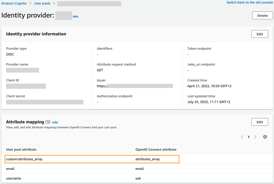


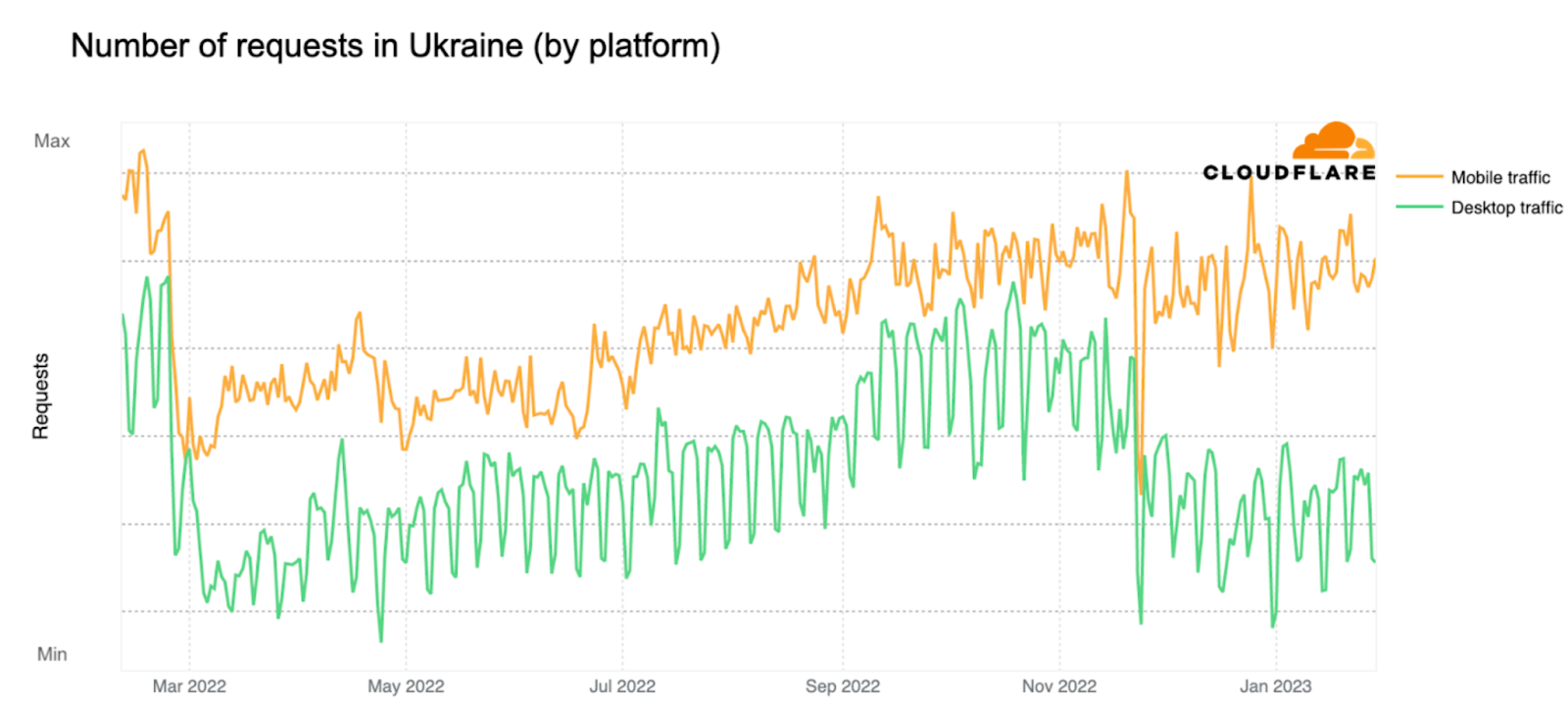
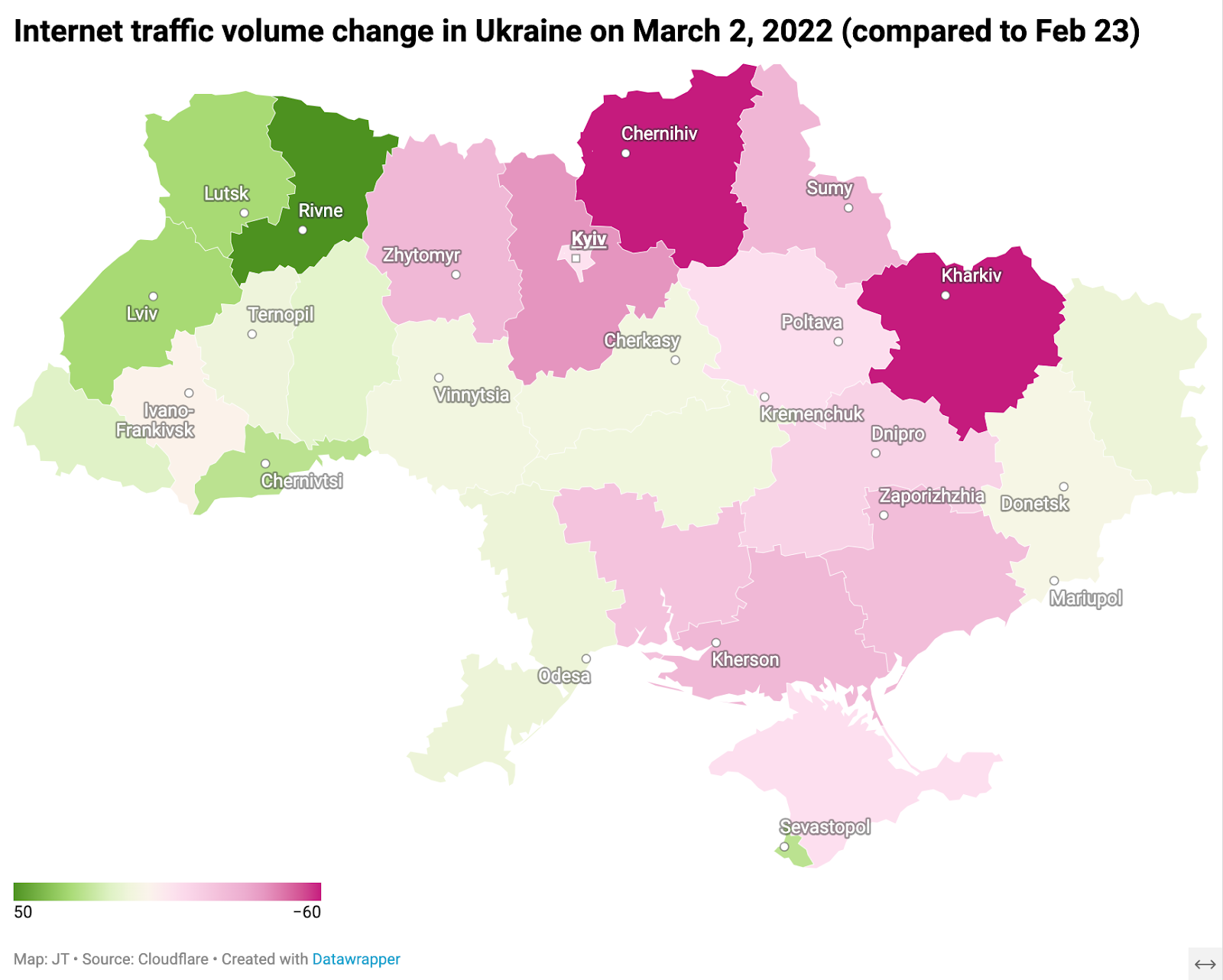
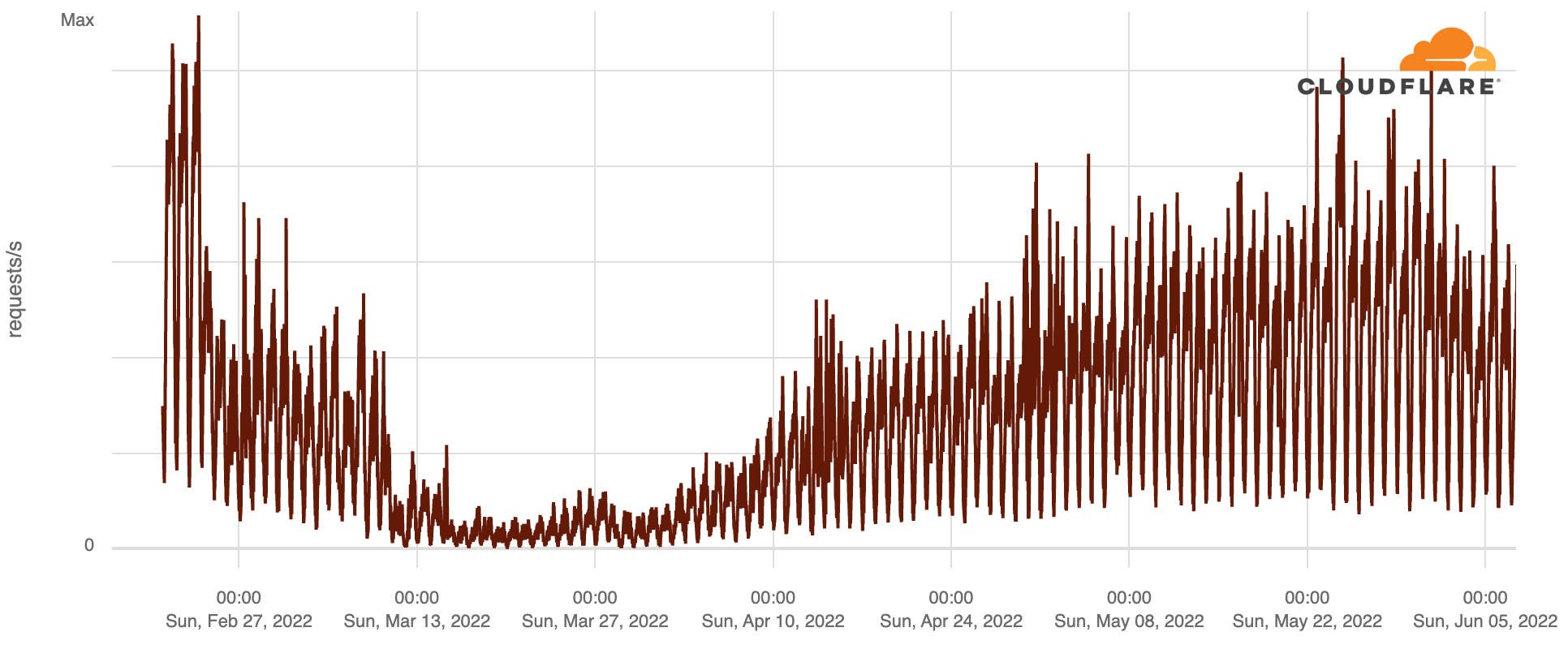
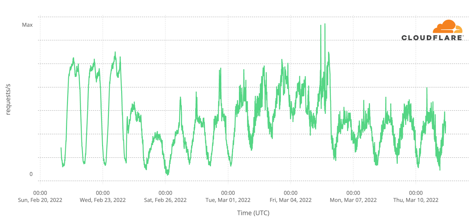
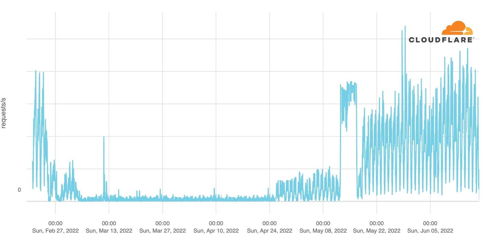
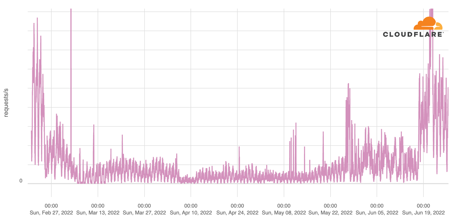
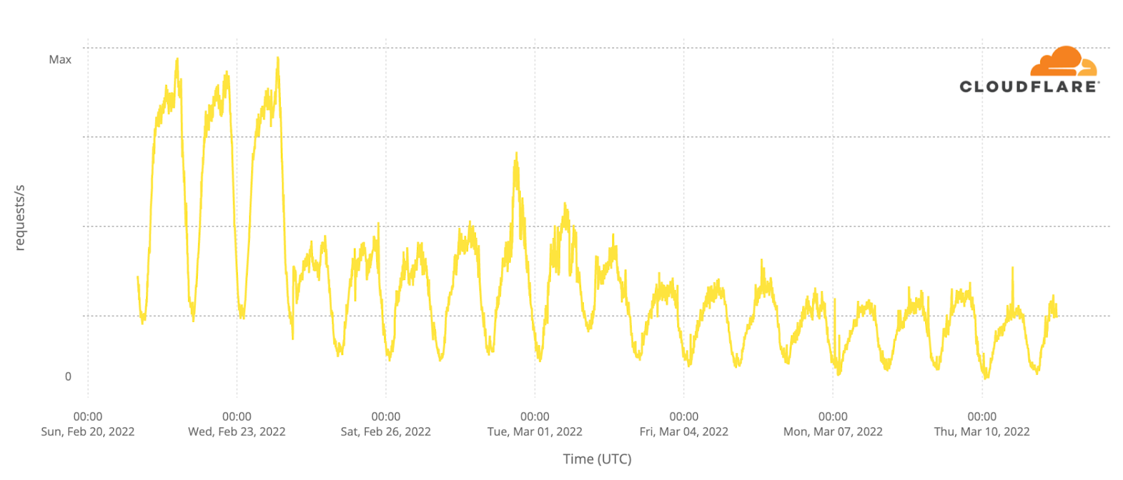
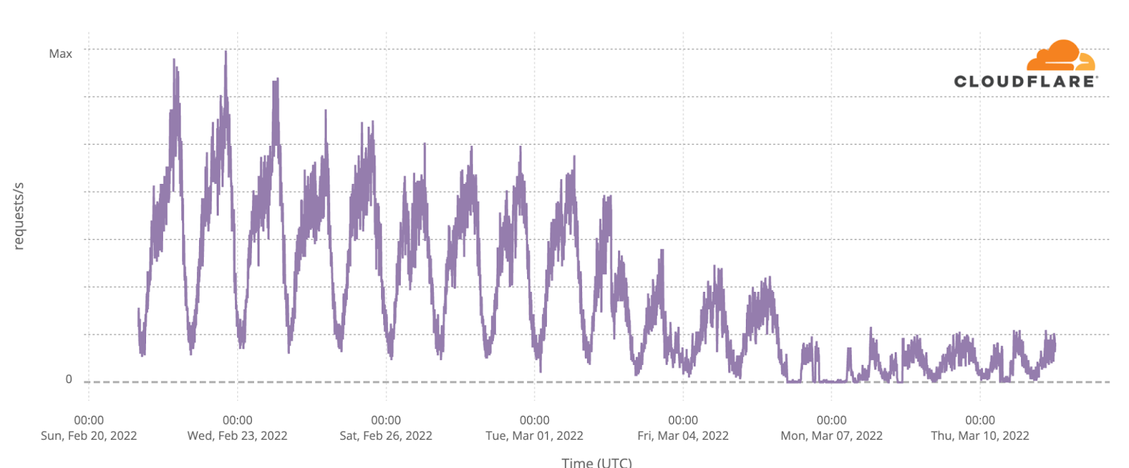
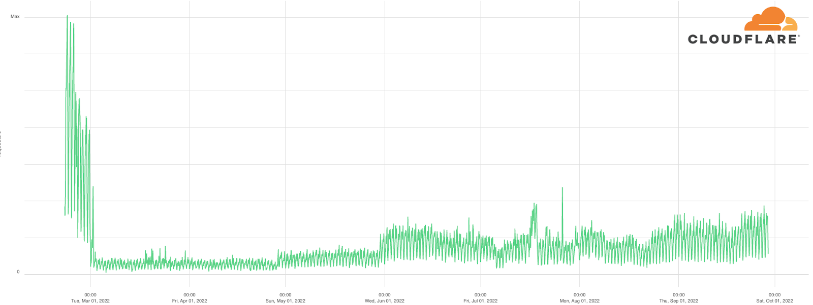
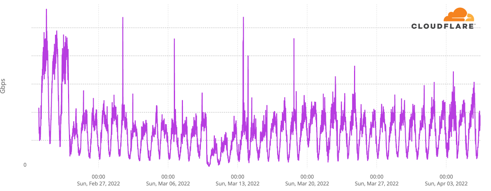
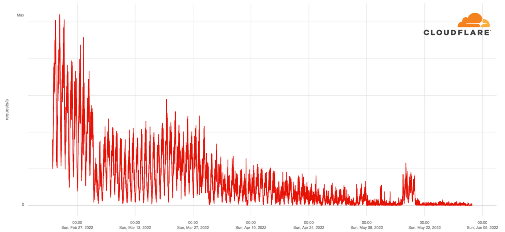
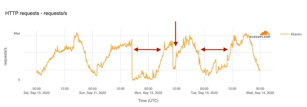


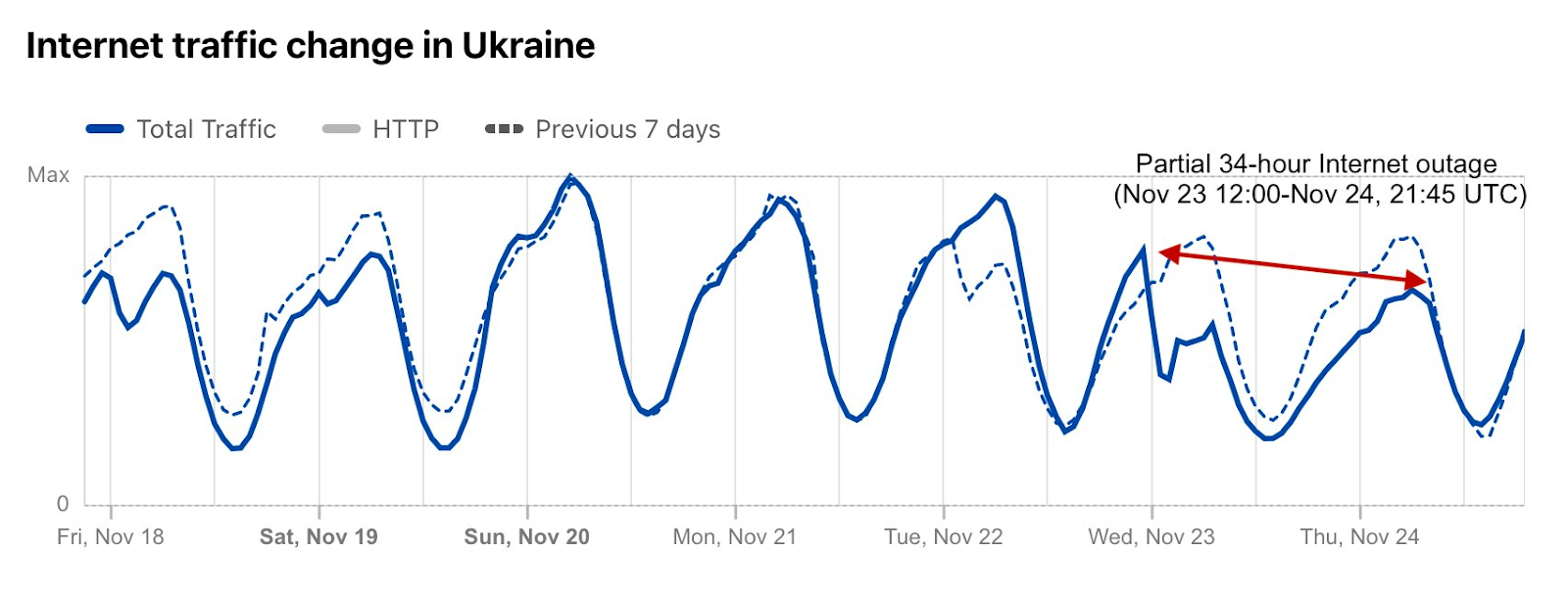
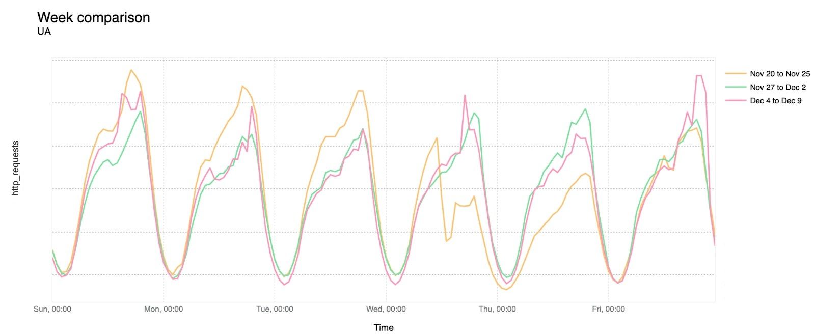


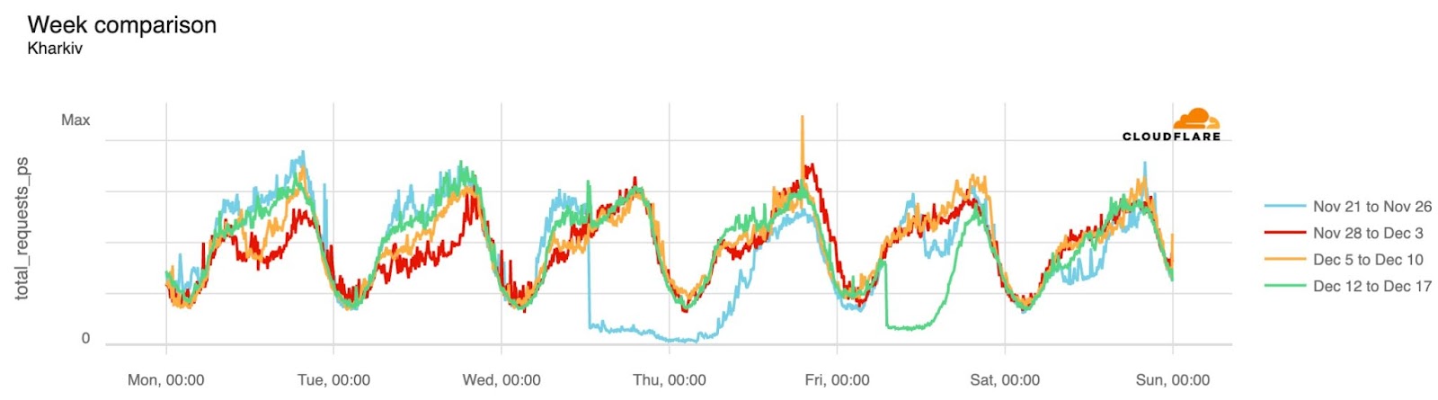
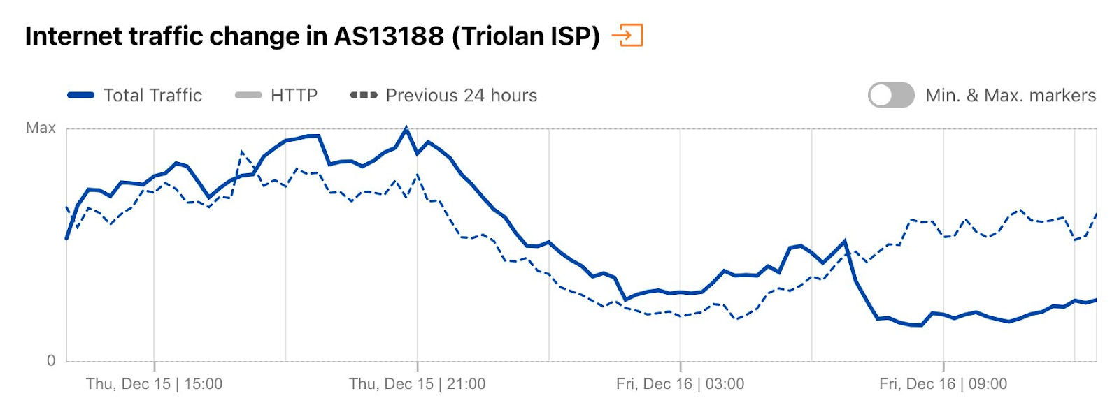
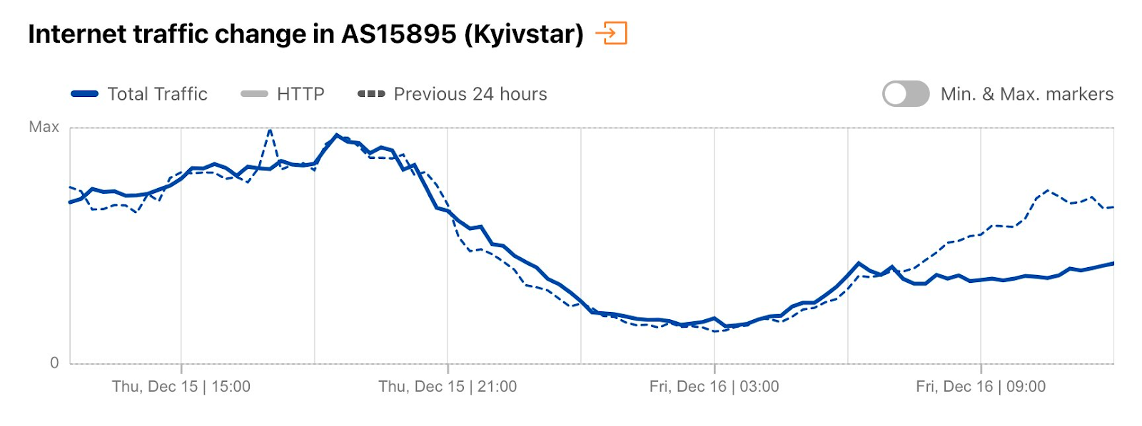


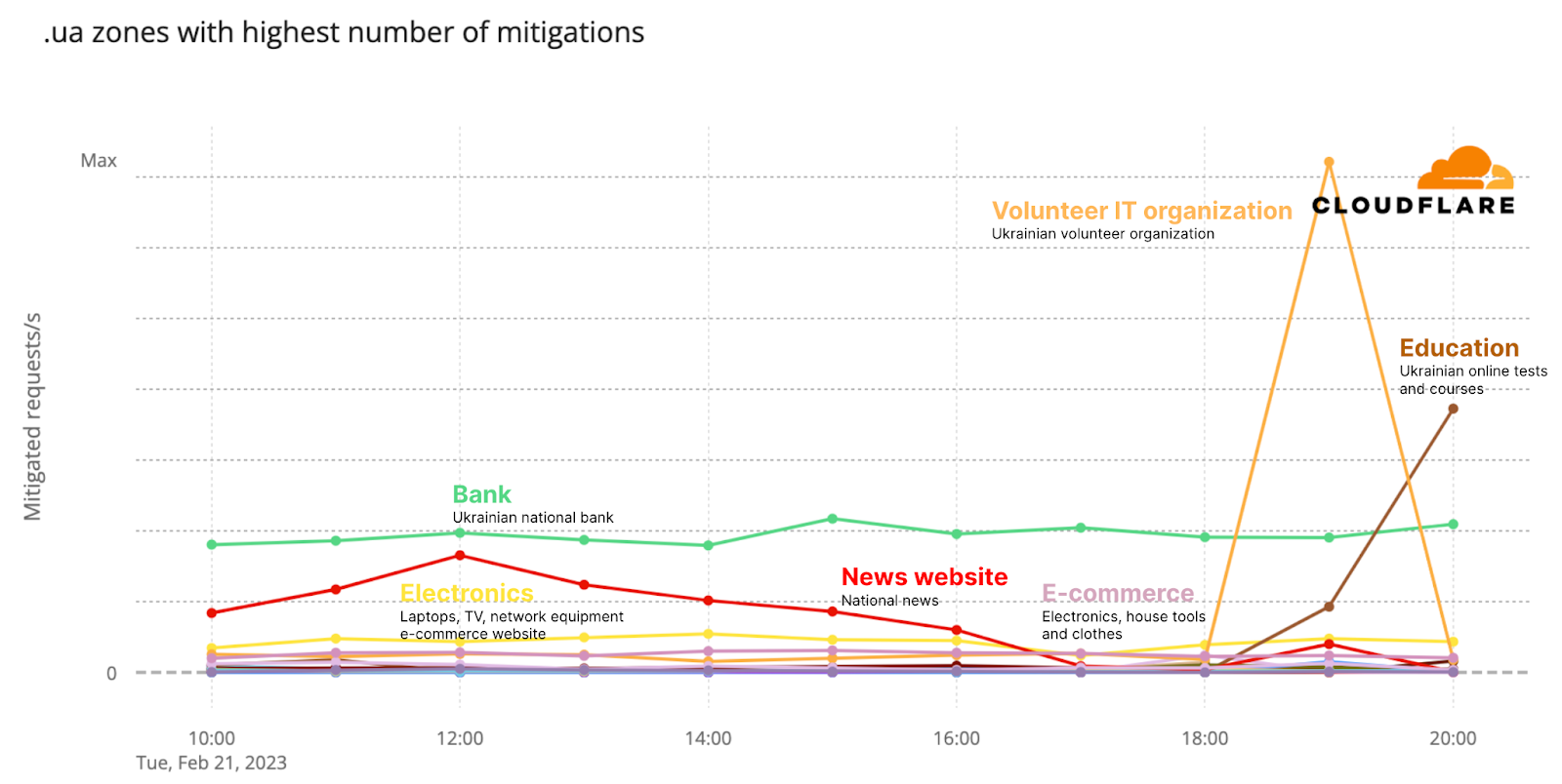


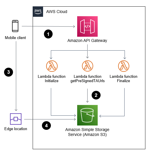


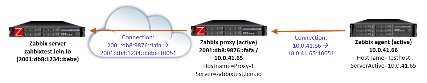
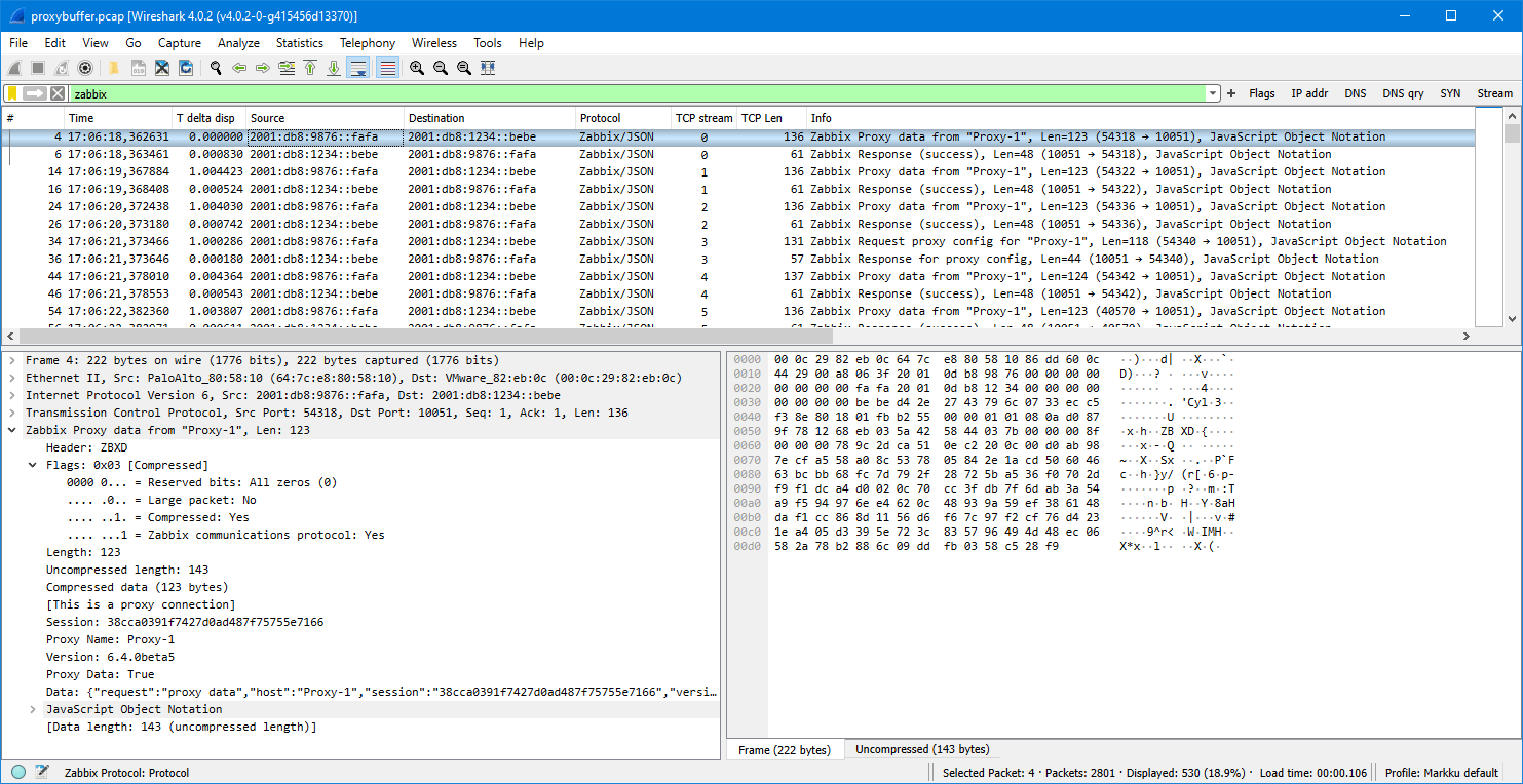

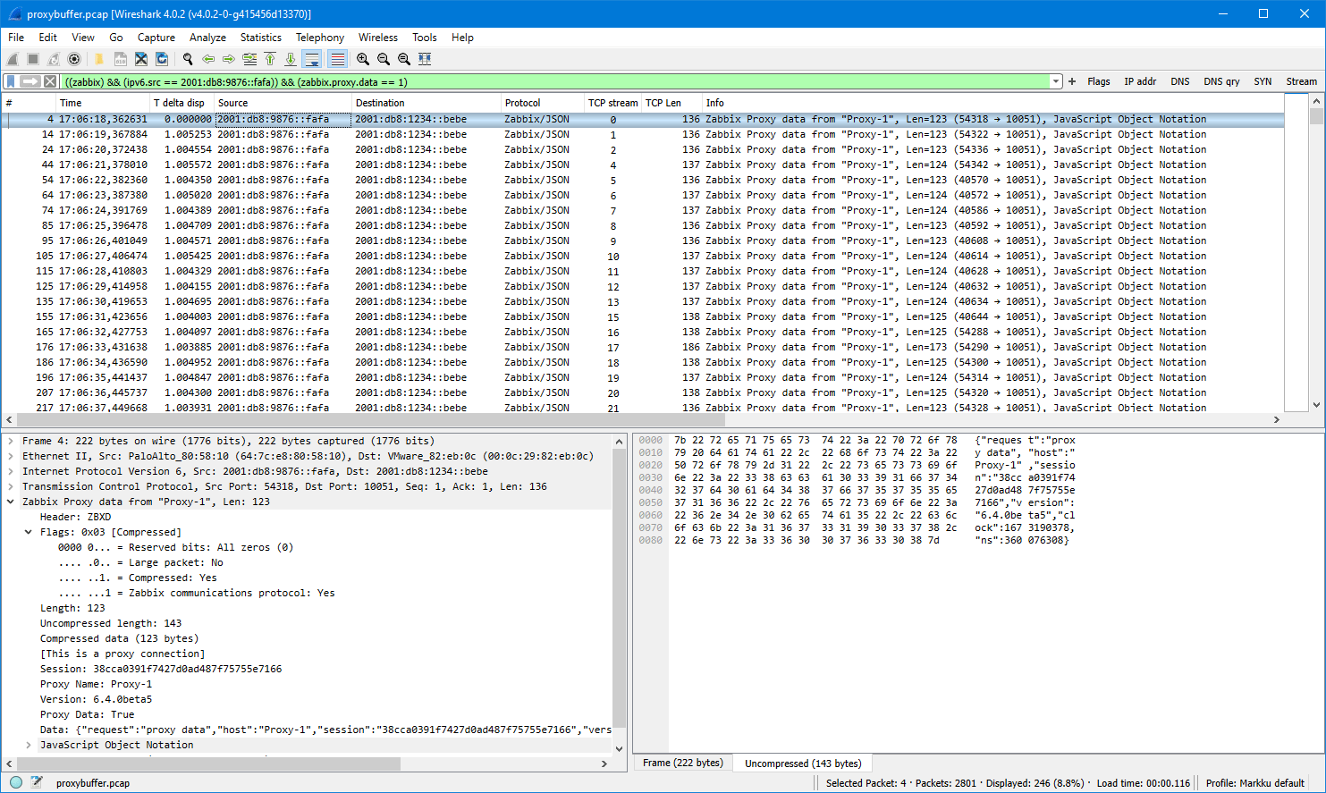


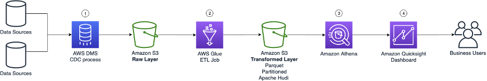
 Olivia Michele is a Data Scientist Lead at Ruparupa, where she has worked in a variety of data roles over the past 5 years, including building and integrating Ruparupa data systems with AWS to improve user experience with data and reporting tools. She is passionate about turning raw information into valuable actionable insights and delivering value to the company.
 Dariswan Janweri P. is a Data Engineer at Ruparupa. He considers challenges or problems as interesting riddles and finds satisfaction in solving them, and even more satisfaction by being able to help his colleagues and friends, “two birds one stone.” He is excited to be a major player in Indonesia’s technology transformation.
 Adrianus Budiardjo Kurnadi is a Senior Solutions Architect at Amazon Web Services Indonesia. He has a strong passion for databases and machine learning, and works closely with the Indonesian machine learning community to introduce them to various AWS Machine Learning services. In his spare time, he enjoys singing in a choir, reading, and playing with his two children.
 Nico Anandito is an Analytics Specialist Solutions Architect at Amazon Web Services Indonesia. He has years of experience working in data integration, data warehouses, and big data implementation in multiple industries. He is certified in AWS data analytics and holds a master’s degree in the data management field of computer science.