The continued growth of AI has fundamentally changed the Internet over the past 24 months. AI is increasingly ubiquitous, and Cloudflare is leaning into the new opportunities and challenges it presents in a big way. This year for Cloudflare’s birthday, we’ve extended our AI Assistant capabilities to help you build new WAF rules, added AI bot traffic insights on Cloudflare Radar, and given customers new AI bot blocking capabilities.
AI Assistant for WAF Rule Builder
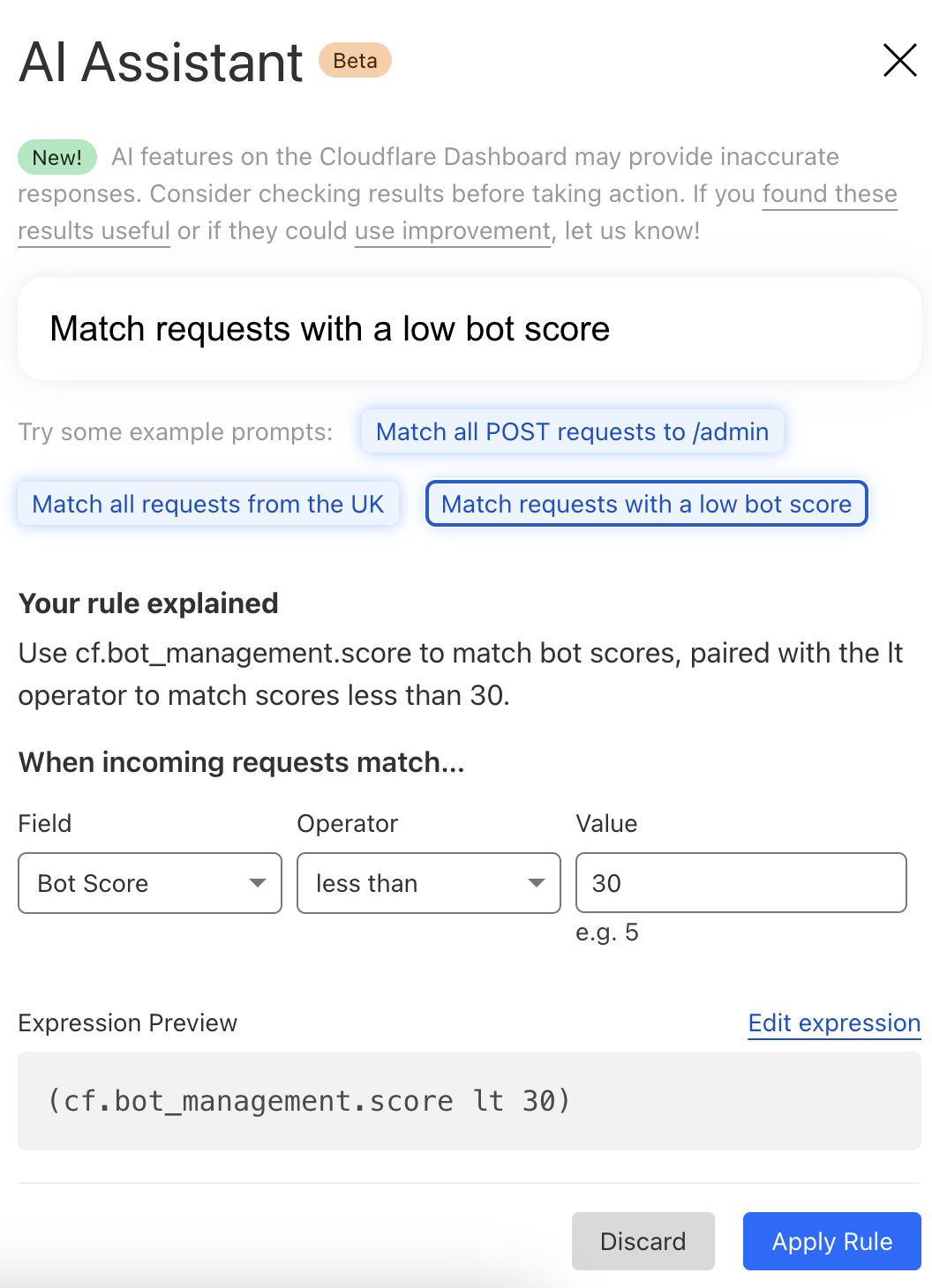
At Cloudflare, we’re always listening to your feedback and striving to make our products as user-friendly and powerful as possible. One area where we’ve heard your feedback loud and clear is in the complexity of creating custom and rate-limiting rules for our Web Application Firewall (WAF). With this in mind, we’re excited to introduce a new feature that will make rule creation easier and more intuitive: the AI Assistant for WAF Rule Builder.
By simply entering a natural language prompt, you can generate a custom or rate-limiting rule tailored to your needs. For example, instead of manually configuring a complex rule matching criteria, you can now type something like, “Match requests with low bot score,” and the assistant will generate the rule for you. It’s not about creating the perfect rule in one step, but giving you a strong foundation that you can build on.
The assistant will be available in the Custom and Rate Limit Rule Builder for all WAF users. We’re launching this feature in Beta for all customers, and we encourage you to give it a try. We’re looking forward to hearing your feedback (via the UI itself) as we continue to refine and enhance this tool to meet your needs.
AI bot traffic insights on Cloudflare Radar
AI platform providers use bots to crawl and scrape websites, vacuuming up data to use for model training. This is frequently done without the permission of, or a business relationship with, the content owners and providers. In July, Cloudflare urged content owners and providers to “declare their AIndependence”, providing them with a way to block AI bots, scrapers, and crawlers with a single click. In addition to this so-called “easy button” approach, sites can provide more specific guidance to these bots about what they are and are not allowed to access through directives in a robots.txt file. Regardless of whether a customer chooses to block or allow requests from AI-related bots, Cloudflare has insight into request activity from these bots, and associated traffic trends over time.
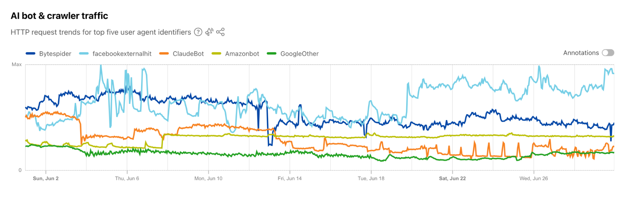
Tracking traffic trends for AI bots can help us better understand their activity over time — which are the most aggressive and have the highest volume of requests, which launch crawls on a regular basis, etc. The new AI bot & crawler traffic graph on Radar’s Traffic page provides insight into these traffic trends gathered over the selected time period for the top known AI bots. The associated list of bots tracked here is based on the ai.robots.txt list, and will be updated with new bots as they are identified. Time series and summary data is available from the Radar API as well. (Traffic trends for the full set of AI bots & crawlers can be viewed in the new Data Explorer.)
Blocking more AI bots
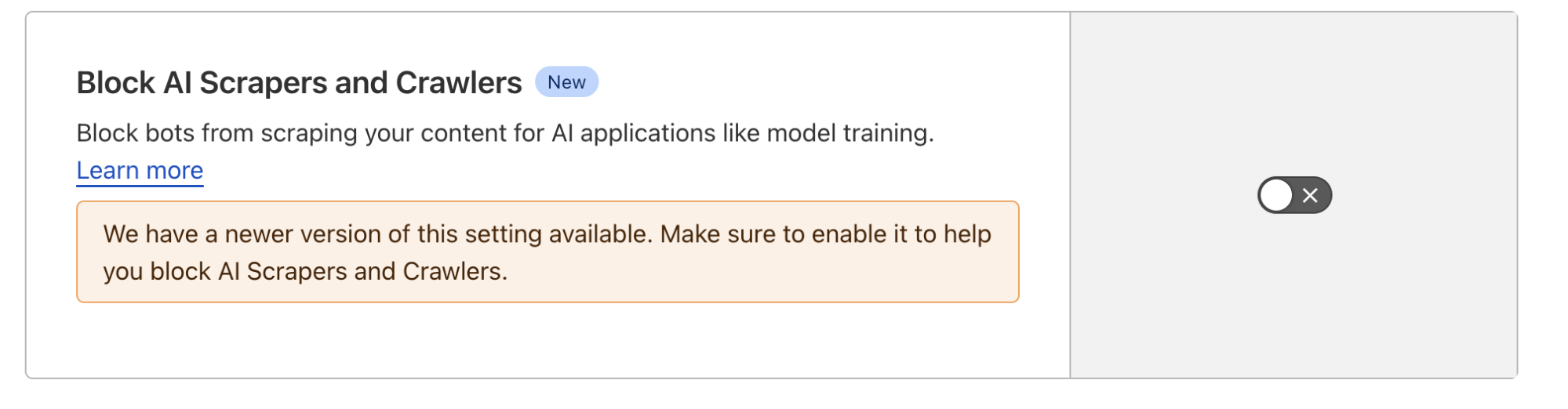
For Cloudflare’s birthday, we’re following up on our previous blog post, Declaring Your AIndependence, with an update on the new detections we’ve added to stop AI bots. Customers who haven’t already done so can simply click the button to block AI bots to gain more protection for their website.
Enabling dynamic updates for the AI bot rule
The old button allowed customers to block verified AI crawlers, those that respect robots.txt and crawl rate, and don’t try to hide their behavior. We’ve added new crawlers to that list, but we’ve also expanded the previous rule to include 27 signatures (and counting) of AI bots that don’t follow the rules. We want to take time to say “thank you” to everyone who took the time to use our “tip line” to point us towards new AI bots. These tips have been extremely helpful in finding some bots that would not have been on our radar so quickly.
For each bot we’ve added, we’re also adding them to our “Definitely automated” definition as well. So, if you’re a self-service plan customer using Super Bot Fight Mode, you’re already protected. Enterprise Bot Management customers will see more requests shift from the “Likely Bot” range to the “Definitely automated” range, which we’ll discuss more below.
Under the hood, we’ve converted this rule logic to a Cloudflare managed rule (the same framework that powers our WAF). This enables our security analysts and engineers to safely push updates to the rule in real-time, similar to how new WAF rule changes are rapidly delivered to ensure our customers are protected against the latest CVEs. If you haven’t logged back into the Bots dashboard since the previous version of our AI bot protection was announced, click the button again to update to the latest protection.
The impact of new fingerprints on the model
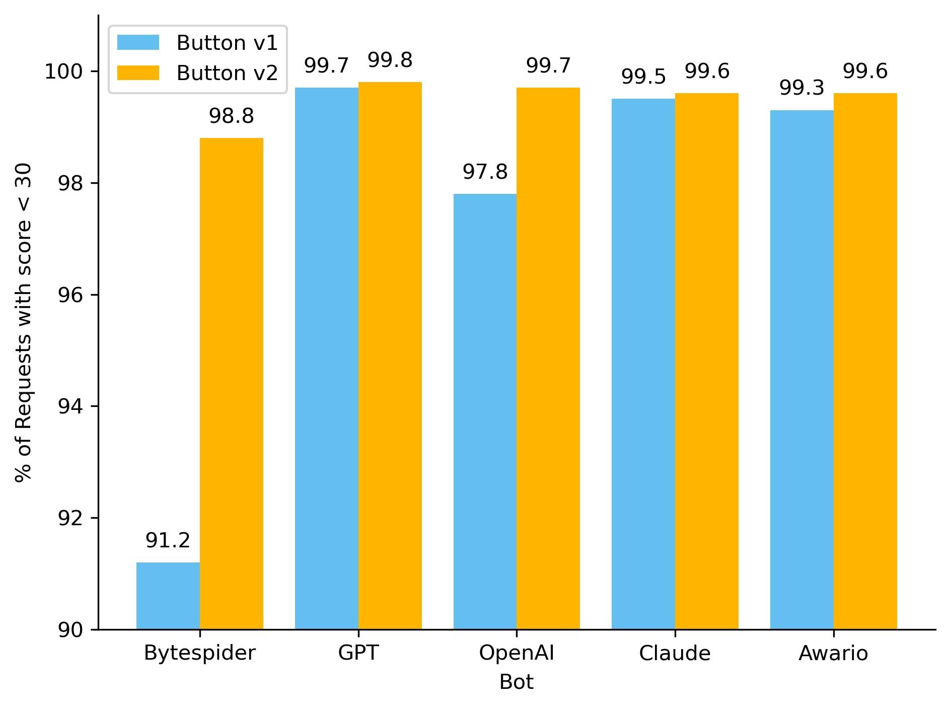
One hidden beneficiary of fingerprinting new AI bots is our ML model. As we’ve discussed before, our global ML model uses supervised machine learning and greatly benefits from more sources of labeled bot data. Below, you can see how well our ML model recognized these requests as automated, before and after we updated the button, adding new rules. To keep things simple, we have shown only the top 5 bots by the volume of requests on the chart. With the introduction of our new managed rule, we have observed an improvement in our detection capabilities for the majority of these AI bots. Button v1 represents the old option that let customers block only verified AI crawlers, while Button v2 is the newly introduced feature that includes managed rule detections.
So how did we make our detections more robust? As we have mentioned before, sometimes a single attribute can give a bot away. We developed a sophisticated set of heuristics tailored to these AI bots, enabling us to effortlessly and accurately classify them as such. Although our ML model was already detecting the vast majority of these requests, the integration of additional heuristics has resulted in a noticeable increase in detection rates for each bot, and ensuring we score every request correctly 100% of the time. Transitioning from a purely machine learning approach to incorporating heuristics offers several advantages, including faster detection times and greater certainty in classification. While deploying a machine learning model is complex and time-consuming, new heuristics can be created in minutes.
The initial launch of the AI bots block button was well-received and is now used by over 133,000 websites, with significant adoption even among our Free tier customers. The newly updated button, launched on August 20, 2024, is rapidly gaining traction. Over 90,000 zones have already adopted the new rule, with approximately 240 new sites integrating it every hour. Overall, we are now helping to protect the intellectual property of more than 146,000 sites from AI bots, and we are currently blocking 66 million requests daily with this new rule. Additionally, we’re excited to announce that support for configuring AI bots protection via Terraform will be available by the end of this year, providing even more flexibility and control for managing your bot protection settings.
Bot behavior
With the enhancements to our detection capabilities, it is essential to assess the impact of these changes to bot activity on the Internet. Since the launch of the updated AI bots block button, we have been closely monitoring for any shifts in bot activity and adaptation strategies. The most basic fingerprinting technique we use to identify AI bot looking for simple user-agent matches. User-agent matches are important to monitor because they indicate the bot is transparently announcing who they are when they’re crawling a website.
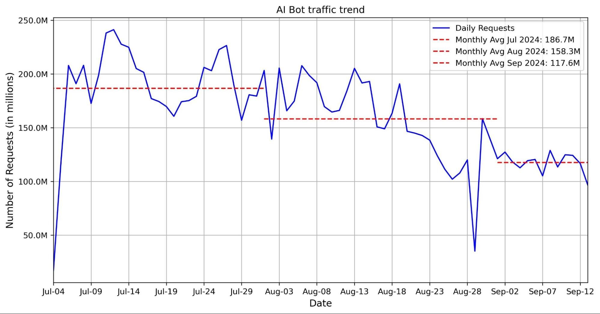
The graph below shows a volume of traffic we label as AI bot over the past two months. The blue line indicates the daily request count, while the red line represents the monthly average number of requests. In the past two months, we have seen an average reduction of nearly 30 million requests, with a decrease of 40 million in the most recent month.This decline coincides with the release of Button v1 and Button v2. Our hypothesis is that with the new AI bots blocking feature, Cloudflare is blocking a majority of these bots, which is discouraging them from crawling.
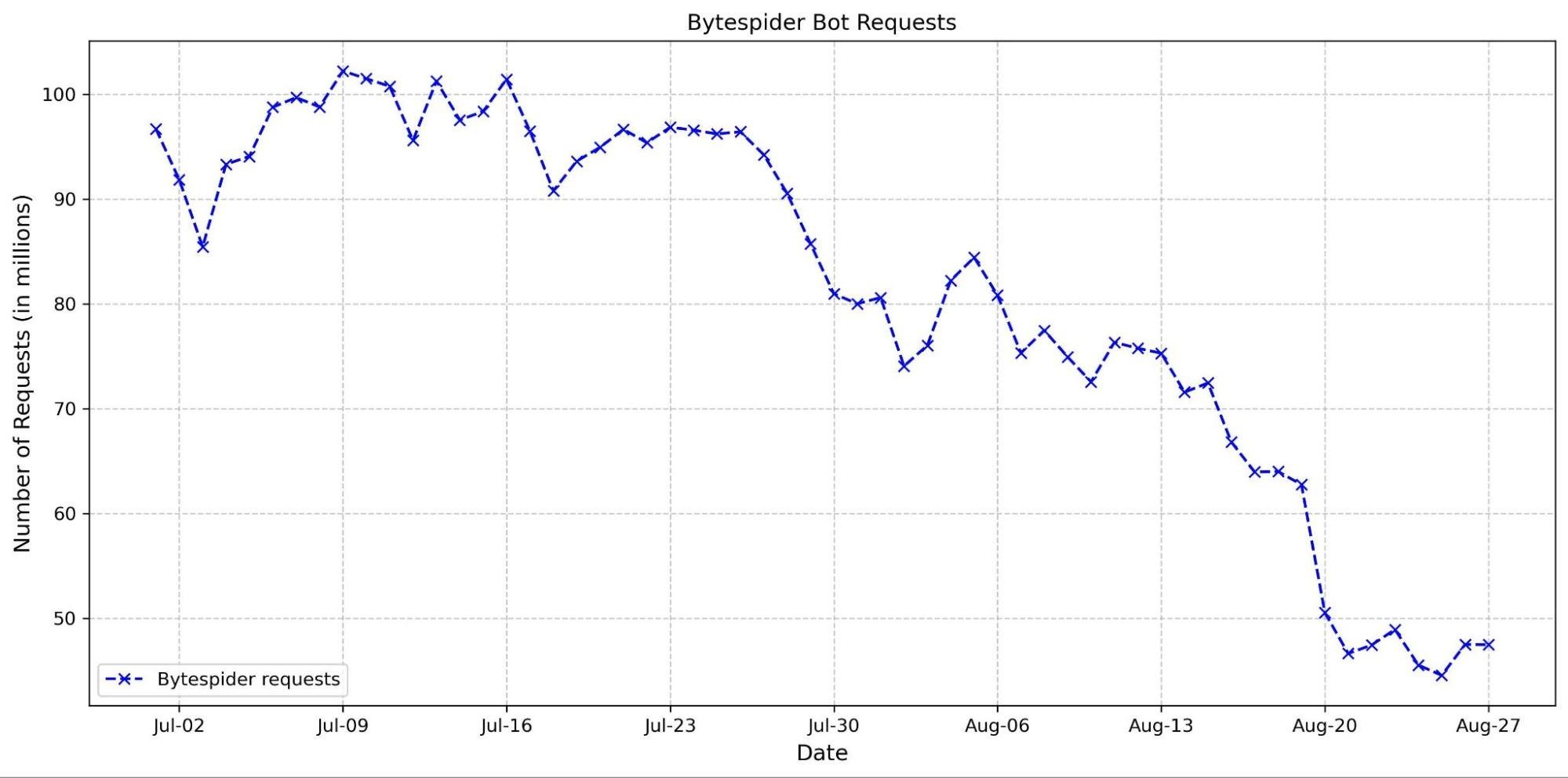
This hypothesis is supported by the observed decline in requests from several top AI crawlers. Specifically, the Bytespider bot reduced its daily requests from approximately 100 million to just 50 million between the end of June and the end of August (see graph below). This reduction could be attributed to several factors, including our new AI bots block button and changes in the crawler’s strategy.
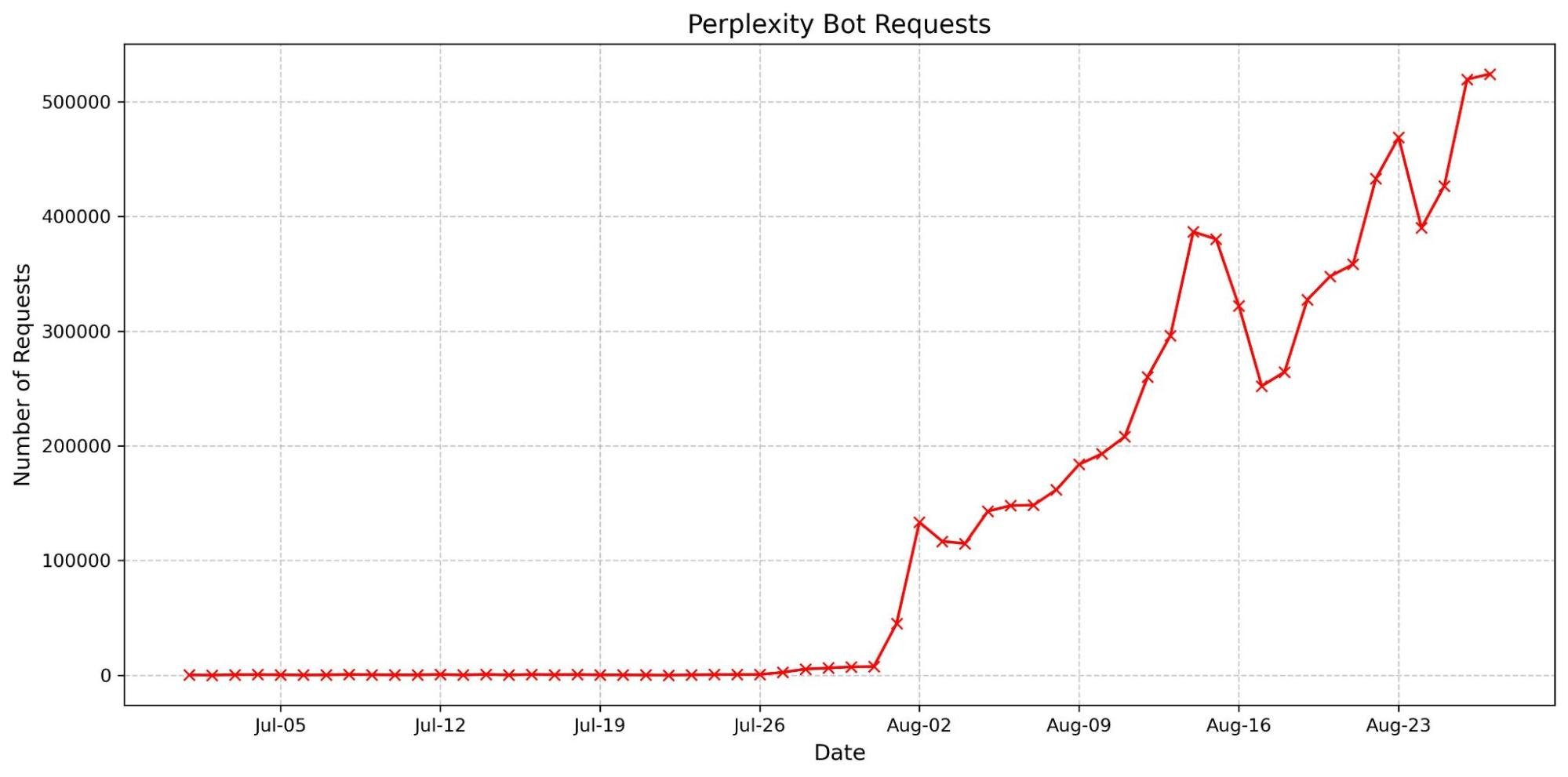
We have also observed an increase in the accountability of some AI crawlers. The most basic fingerprinting technique we use to identify AI bot looking for simple user-agent matches. User-agent matches are important to monitor because they indicate the bot is transparently announcing who they are when they’re crawling a website. These crawlers are now more frequently using their agents, reflecting a shift towards more transparent and responsible behavior. Notably, there has been a dramatic surge in the number of requests from the Perplexity user agent. This increase might be linked to previous accusationsthat Perplexity did not properly present its user agent, which could have prompted a shift in their approach to ensure better identification and compliance.
These trends suggest that our updates are likely affecting how AI crawlers interact with content. We will continue to monitor AI bot activity to help users control who accesses their content and how. By keeping a close watch on emerging patterns, we aim to provide users with the tools and insights needed to make informed decisions about managing their traffic.
Wrap up
We’re excited to continue to explore the AI landscape, whether we’re finding more ways to make the Cloudflare dashboard usable or new threats to guard against. Our AI insights on Radar update in near real-time, so please join us in watching as new trends emerge and discussing them in the Cloudflare Community.
We’ve been working on something new — a platform for running containers across Cloudflare’s network. We already use it in production for Workers AI, Workers Builds, Remote Browsing Isolation, and the Browser Rendering API. Today, we want to share an early look at how it’s built, why we built it, and how we use it ourselves.
In 2024, Cloudflare Workers celebrates its 7th birthday. When we first announced Workers, it was a completely new model for running compute in a multi-tenant way — on isolates, as opposed to containers. While, at the time, Workers was a pretty bare-bones functions-as-a-service product, we took a big bet that this was going to become the way software was going to be written going forward. Since introducing Workers, in addition to expanding our developer products in general to include storage and AI, we have been steadily adding more compute capabilities to Workers:
With each of these, we’ve faced a question — can we build this natively into the platform, in a way that removes, rather than adds complexity? Can we build it in a way that lets developers focus on building and shipping, rather than managing infrastructure, so that they don’t have to be a distributed systems engineer to build distributed systems?
In each instance, the answer has been YES. We try to solve problems in a way that simplifies things for developers in the long run, even if that is the harder path for us to take ourselves. If we didn’t, you’d be right to ask — why not self-host and manage all of this myself? What’s the point of the cloud if I’m still provisioning and managing infrastructure? These are the questions many are asking today about the earlier generation of cloud providers.
Pushing ourselves to build platform-native products and features helped us answer this question. Particularly because some of these actually use containers behind the scenes, even though as a developer you never interact with or think about containers yourself.
If you’ve used AI inference on GPUs with Workers AI, spun up headless browsers with Browser Rendering, or enqueued build jobs with the new Workers Builds, you’ve run containers on our network, without even knowing it. But to do so, we needed to be able to run untrusted code across Cloudflare’s network, outside a v8 isolate, in a way that fits what we promise:
You shouldn’t have to think about regions or data centers. Routing, scaling, load balancing, scheduling, and capacity are our problem to solve, not yours, with tools like Smart Placement.
You should be able to build distributed systems without being a distributed systems engineer.
Every millisecond matters — Cloudflare has to be fast.
There wasn’t an off-the-shelf container platform that solved for what we needed, so we built it ourselves — from scheduling to IP address management, pulling and caching images, to improving startup times and more. Our container platform powers many of our newest products, so we wanted to share how we built it, optimized it, and well, you can probably guess what’s next.
Global scheduling — “The Network is the Computer”
Cloudflare serves the entire world — region: earth. Rather than asking developers to provision resources in specific regions, data centers and availability zones, we think “The Network is the Computer”. When you build on Cloudflare, you build software that runs on the Internet, not just in a data center.
When we started working on this, Cloudflare’s architecture was to just run every service via systemd on every server (we call them “metals” — we run our own hardware), allowing all services to take advantage of new capacity we add to our network. That fits running NGINX and a few dozen other services, but cannot fit a world where we need to run many thousands of different compute heavy, resource hungry workloads. We’d run out of space just trying to load all of them! Consider a canonical AI workload — deploying Llama 3.1 8B to an inference server. If we simply ran a Llama 3.1 8B service on every Cloudflare metal, we’d have no flexibility to use GPUs for the many other models that Workers AI supports.
We needed something that would allow us to still take advantage of the full capacity of Cloudflare’s entire network, not just the capacity of individual machines. And ideally not put that burden on the developer.
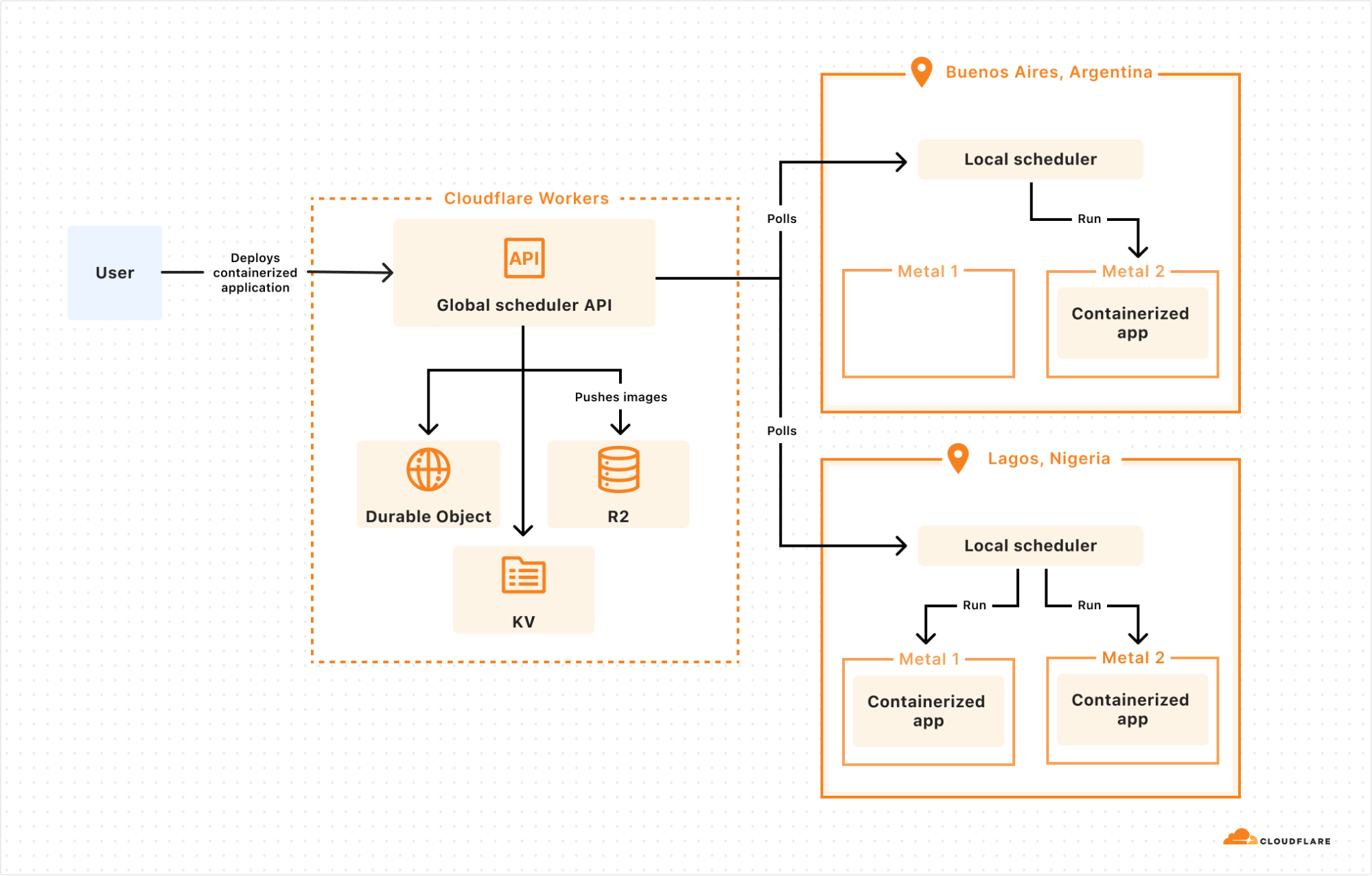
The answer: we built a control plane on our own Developer Platform that lets us schedule a container anywhere on Cloudflare’s Network:
The global scheduler is built on Cloudflare Workers, Durable Objects, and KV, and decides which Cloudflare location to schedule the container to run in. Each location then runs its own scheduler, which decides which metals within that location to schedule the container to run on. Location schedulers monitor compute capacity, and expose this to the global scheduler. This allows Cloudflare to dynamically place workloads based on capacity and hardware availability (e.g. multiple types of GPUs) across our network.
Why does global scheduling matter?
When you run compute on a first generation cloud, the “contract” between the developer and the platform is that the developer must specify what runs where. This is regional scheduling, the status quo.
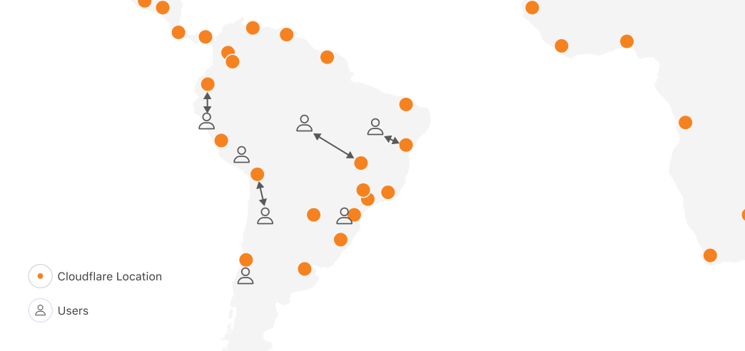
Let’s imagine for a second if we applied regional scheduling to running compute on Cloudflare’s network, with locations in 330+ cities, across 120+ countries. One of the obvious reasons people tell us they want to run on Cloudflare is because we have compute in places where others don’t, within 50ms of 95% of the world’s Internet-connected population. In South America, other clouds have one region in one city. Cloudflare has 19:
Running anywhere means you can be faster, highly available, and have more control over data location. But with regional scheduling, the more locations you run in, the more work you have to do. You configure and manage load balancing, routing, auto-scaling policies and more. Balancing performance and cost in a multi-region setup is literally a full-time job (or more) at most companies who have reached meaningful scale on traditional clouds.
But most importantly, no matter what tools you bring, you were the one who told the cloud provider, “run this container over here”. The cloud platform can’t move it for you, even if moving it would make your workload faster. This prevents the platform from adding locations, because for each location, it has to convince developers to take action themselves to move their compute workloads to the new location. Each new location carries a risk that developers won’t migrate workloads to it, or migrate too slowly, delaying the return on investment.
Global scheduling means Cloudflare can add capacity and use it immediately, letting you benefit from it. The “contract” between us and our customers isn’t tied to a specific datacenter or region, so we have permission to move workloads around to benefit customers. This flexibility plays an essential role in all of our own uses of our container platform, starting with GPUs and AI.
GPUs everywhere: Scheduling large images with Workers AI
In late 2023, we launched Workers AI, which provides fast, easy to use, and affordable GPU-backed AI inference.
The more efficiently we can use our capacity, the better pricing we can offer. And the faster we can make changes to which models run in which Cloudflare locations, the closer we can move AI inference to the application, lowering Time to First Token (TTFT). This also allows us to be more resilient to spikes in inference requests.
AI models that rely on GPUs present three challenges though:
Models have different GPU memory needs. GPU memory is the most scarce resource, and different GPUs have different amounts of memory.
Not all container runtimes, such as Firecracker, support GPU drivers and other dependencies.
AI models, particularly LLMs, are very large. Even a smaller parameter model, like @cf/meta/llama-3.1-8b-instruct, is at least 5 GB. The larger the model, the more bytes we need to pull across the network when scheduling a model to run in a new location.
Let’s dive into how we solved each of these…
First, GPU memory needs. The global scheduler knows which Cloudflare locations have blocks of GPU memory available, and then delegates scheduling the workload on a specific metal to the local scheduler. This allows us to prioritize placement of AI models that use a large amount of GPU memory, and then move smaller models to other machines in the same location. By doing this, we maximize the overall number of locations that we run AI models in, and maximize our efficiency.
Second, container runtimes and GPU support. Thankfully, from day one we built our container platform to be runtime agnostic. Using a runtime agnostic scheduler, we’re able to support gVisor, Firecracker microVMs, and traditional VMs with QEMU. We are also evaluating adding support for another one: cloud-hypervisor which is based on rust-vmm and has a few compelling advantages for our use case:
vhost-user-net support, enabling high throughput between the host network interface and the VM
vhost-user-blk support, adding flexibility to introduce novel network-based storage backed by other Cloudflare Workers products
all the while being a smaller codebase than QEMU and written in a memory-safe language
Our goal isn’t to build a platform that makes you as the developer choose between runtimes, and ask, “should I use Firecracker or gVisor”. We needed this flexibility in order to be able to run workloads with different needs efficiently, including workloads that depend on GPUs. gVisor has GPU support, while Firecracker microVMs currently does not.
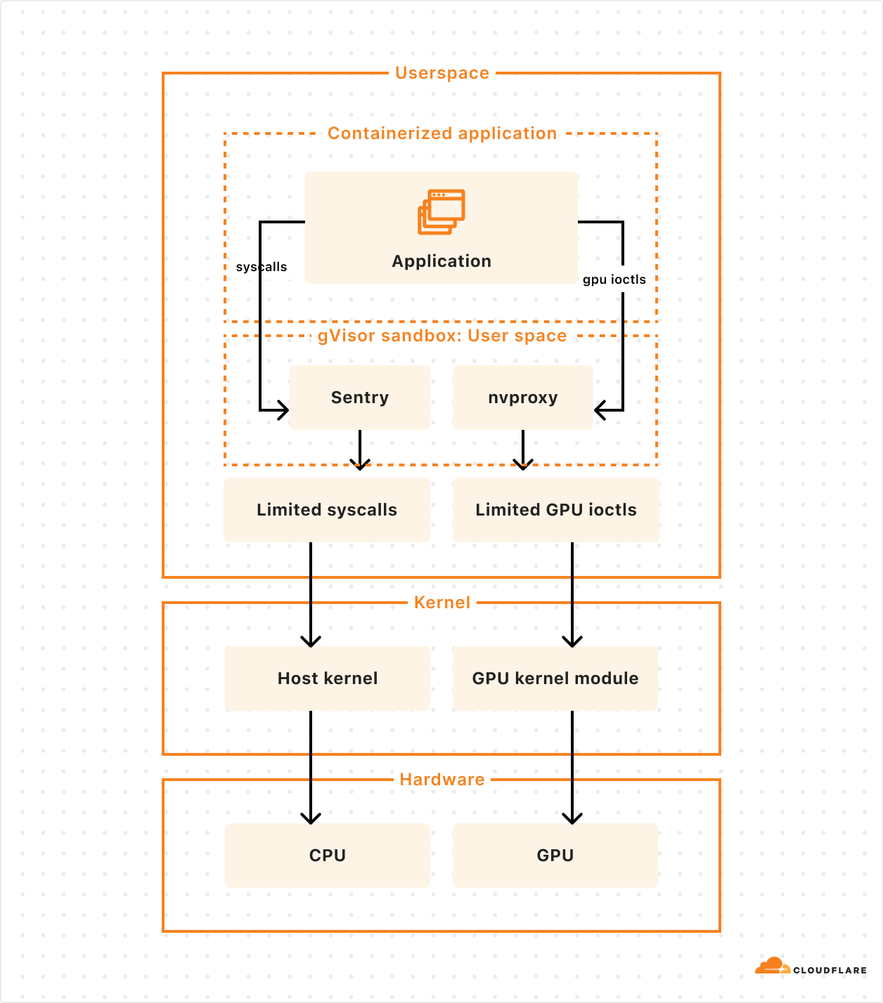
gVisor’s main component is an application kernel (called Sentry) that implements a Linux-like interface but is written in a memory-safe language (Go) and runs in userspace. It works by intercepting application system calls and acting as the guest kernel, without the need for translation through virtualized hardware.
The resource footprint of a containerized application running on gVisor is lower than a VM because it does not require managing virtualized hardware and booting up a kernel instance. However, this comes at the price of reduced application compatibility and higher per-system call overhead.
To add GPU support, the Google team introduced nvproxy which works using the same principles as described above for syscalls: it intercepts ioctls destined to the GPU and proxies a subset to the GPU kernel module.
To solve the third challenge, and make scheduling fast with large models, we weren’t satisfied with the status quo. So we did something about it.
Docker pull was too slow, so we fixed it (and cut the time in half)
Many of the images we need to run for AI inference are over 15 GB. Specialized inference libraries and GPU drivers add up fast. For example, when we make a scheduling decision to run a fresh container in Tokyo, naively running docker pull to fetch the image from a storage bucket in Los Angeles would be unacceptably slow. And scheduling speed is critical to being able to scale up and down in new locations in response to changes in traffic.
We had 3 essential requirements:
Pulling and pushing very large images should be fast
We should not rely on a single point of failure
Our teams shouldn’t waste time managing image registries
We needed globally distributed storage, so we used R2. We needed the highest cache hit rate possible, so we used Cloudflare’s Cache, and will soon use Tiered Cache. And we needed a fast container image registry that we could run everywhere, in every Cloudflare location, so we built and open-sourced serverless-registry, which is built on Workers. You can deploy serverless-registry to your own Cloudflare account in about 5 minutes. We rely on it in production.
This is fast, but we can be faster. Our performance bottleneck was, somewhat surprisingly, docker push. Docker uses gzip to compress and decompress layers of images while pushing and pulling. So we started using Zstandard (zstd) instead, which compresses and decompresses faster, and results in smaller compressed files.
In order to build, chunk, and push these images to the R2 registry, we built a custom CLI tool that we use internally in lieu of running docker build and docker push. This makes it easy to use zstd and split layers into 500 MB chunks, which allows uploads to be processed by Workers while staying under body size limits.
Using our custom build and push tool doubled the speed of image pulls. Our 30 GB GPU images now pull in 4 minutes instead of 8. We plan on open sourcing this tool in the near future.
Anycast is the gift that keeps on simplifying — Virtual IPs and the Global State Router
We still had another challenge to solve. And yes, we solved it with anycast. We’re Cloudflare, did you expect anything else?
First, a refresher — Cloudflare operates Unimog, a Layer 4 load balancer that handles all incoming Cloudflare traffic. Cloudflare’s network uses anycast, which allows a single IP address to route requests to a variety of different locations. For most Cloudflare services with anycast, the given IP address will route to the nearest Cloudflare data center, reducing latency. Since Cloudflare runs almost every service in every data center, Unimog can simply route traffic to any Cloudflare metal that is online and has capacity, without needing to map traffic to a specific service that runs on specific metals, only in some locations.
The new compute-heavy, GPU-backed workloads we were taking on forced us to confront this fundamental “everything runs everywhere” assumption. If we run a containerized workflow in 20 Cloudflare locations, how does Unimog know which locations, and which metals, it runs in? You might say “just bring your own load balancer” — but then what happens when you make scheduling decisions to migrate a workload between locations, scale up, or scale down?
Anycast is foundational to how we build fast and simple products on our network, and we needed a way to keep building new types of products this way — where a team can deploy an application, get back a single IP address, and rely on the platform to balance traffic, taking load, container health, and latency into account, without extra configuration. We started letting teams use the container platform without solving this, and it was painfully clear that we needed to do something about it.
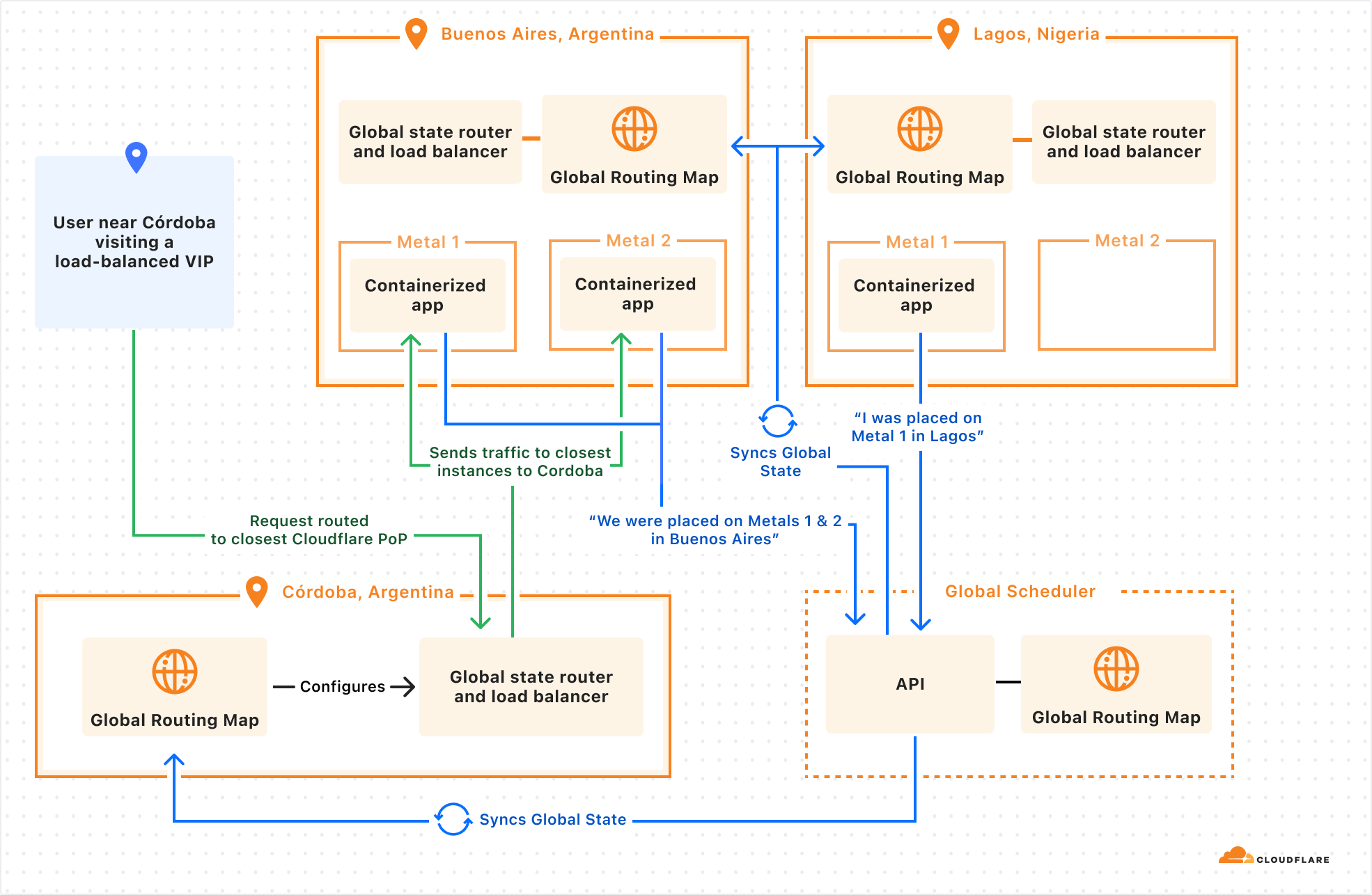
So we started integrating directly into our networking stack, building a sidecar service to Unimog. We’ll call this the Global State Router. Here’s how it works:
An eyeball makes a request to a virtual IP address issued by Cloudflare
Request sent to the best location as determined by BGP routing. This is anycast routing.
A small eBPF program sits on the main networking interface and ensures packets bound to a virtual IP address are handled by the Global State Router.
The main Global State Router program contains a mapping of all anycast IPs addresses to potential end destination container IP addresses. It updates this mapping based on container health, readiness, distance, and latency. Using this information, it picks a best-fit container.
Packets are forwarded at the L4 layer.
When a target container’s server receives a packet, its own Global State Router program intercepts the packet and routes it to the local container.
This might sound like just a lower level networking detail, disconnected from developer experience. But by integrating directly with Unimog, we can let developers:
Push a containerized application to Cloudflare.
Provide constraints, health checks, and load metrics that describe what the application needs.
Delegate scheduling and scaling many containers across Cloudflare’s network.
Get back a single IP address that can be used everywhere.
We’re actively working on this, and are excited to continue building on Cloudflare’s anycast capabilities, and pushing to keep the simplicity of running “everywhere” with new categories of workloads.
Our container platform actually started because of a very specific challenge, running Remote Browser Isolation across our network. Remote Browser Isolation provides Chromium browsers that run on Cloudflare, in containers, rather than on the end user’s own computer. Only the rendered output is sent to the end user. This provides a layer of protection against zero-day browser vulnerabilities, phishing attacks, and ransomware.
Location is critical — people expect their interactions with a remote browser to feel just as fast as if it ran locally. If the server is thousands of miles away, the remote browser will feel slow. Running across Cloudflare’s network of over 330 locations means the browser is nearly always as close to you as possible.
Imagine a user in Santiago, Chile, if they were to access a browser running in the same city, each interaction would incur negligible additional latency. Whereas a browser in Buenos Aires might add 21 ms, São Paulo might add 48 ms, Bogota might add 67 ms, and Raleigh, NC might add 128 ms. Where the container runs significantly impacts the latency of every user interaction with the browser, and therefore the experience as a whole.
It’s not just browser isolation that benefits from running near the user: WebRTC servers stream video better, multiplayer games have less lag, online advertisements can be served faster, financial transactions can be processed faster. Our container platform lets us run anything we need to near the user, no matter where they are in the world.
Using spare compute — “off-peak” jobs for Workers CI/CD builds
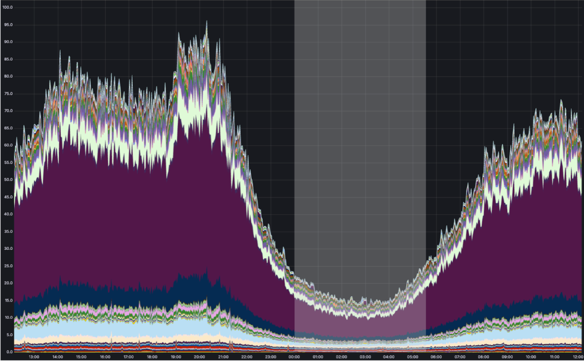
At any hour of the day, Cloudflare has many CPU cores that sit idle. This is compute power that could be used for something else.
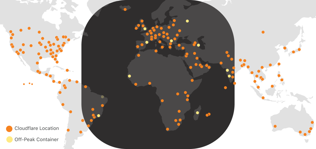
Via anycast, most of Cloudflare’s traffic is handled as close as possible to the eyeball (person) that requested it. Most of our traffic originates from eyeballs. And the eyeballs of (most) people are closed and asleep between midnight and 5:00 AM local time. While we use our compute capacity very efficiently during the daytime in any part of the world, overnight we have spare cycles. Consider what a map of the world looks like at night-time in Europe and Africa:
As shown above, we can run containers during “off-peak” in Cloudflare locations receiving low traffic at night. During this time, the CPU utilization of a typical Cloudflare metal looks something like this:
We have many “background” compute workloads at Cloudflare. These are workloads that don’t actually need to run close to the eyeball because there is no eyeball waiting on the request. The challenge is that many of these workloads require running untrusted code — either a dependency on open-source code that we don’t trust enough to run outside of a sandboxed environment, or untrusted code that customers deploy themselves. And unlike Cron Triggers, which already make a best-effort attempt to use off-peak compute, these other workloads can’t run in v8 isolates.
On Builder Day 2024, we announced Workers Builds in open beta. You connect your Worker to a git repository, and Cloudflare builds and deploys your Worker each time you merge a pull request. Workers Builds run on our containers platform, using otherwise idle “off-peak” compute, allowing us to offer lower pricing, and hold more capacity for unexpected spikes in traffic in Cloudflare locations during daytime hours when load is highest. We preserve our ability to serve requests as close to the eyeball as possible where it matters, while using the full compute capacity of our network.
We developed a purpose-built API for these types of jobs. The Workers Builds service has zero knowledge of where Cloudflare has spare compute capacity on its network — it simply schedules an “off-peak” job to run on the containers platform, by defining a scheduling policy:
scheduling_policy: "off-peak"
Making off-peak jobs faster with prewarmed images
Just because a workload isn’t “eyeball-facing” doesn’t mean speed isn’t relevant. When a build job starts, you still want it to start as soon as possible.
Each new build requires a fresh container though, and we must avoid reusing containers to provide strong isolation between customers. How can we keep build job start times low, while using a new container for each job without over-provisioning?
We prewarm servers with the proper image.
Before a server becomes eligible to receive an “off peak” job, the container platform instructs it to download the correct image. Once the image is downloaded and cached locally, new containers can start quickly in a Firecracker VM after receiving a request for a new build. When a build completes, we throw away the container, and start the next build using a fresh container based on the prewarmed image.
Without prewarming, pulling and unpacking our Workers Build images would take roughly 75 seconds. With prewarming, we’re able to spin up a new container in under 10 seconds. We expect this to get even faster as we introduce optimizations like pre-booting images before new runs, or Firecracker snapshotting, which can restore a VM in under 200ms.
Workers and containers, better together
As more of our own engineering teams rely on our containers platform in production, we’ve noticed a pattern: they want a deeper integration with Workers.
We plan to give it to them.
Let’s take a look at a project deployed on our container platform already, Key Transparency. If the container platform were highly integrated with Workers, what would this team’s experience look like?
Cloudflare regularly audits changes to public keys used by WhatsApp for encrypting messages between users. Much of the architecture is built on Workers, but there are long-running compute-intensive tasks that are better suited for containers.
We don’t want our teams to have to jump through hoops to deploy a container and integrate with Workers. They shouldn’t have to pick specific regions to run in, figure out scaling, expose IPs and handle IP updates, or set up Worker-to-container auth.
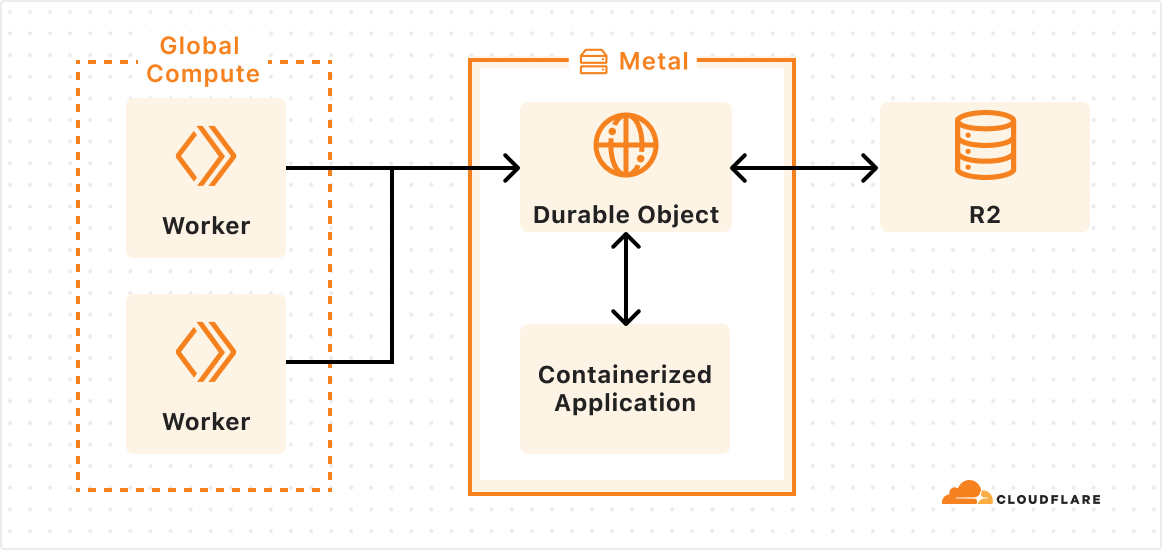
We’re still exploring many different ideas and API designs, and we want your feedback. But let’s imagine what it might look like to use Workers, Durable Objects and Containers together.
In this case, an outer layer of Workers handles most business logic and ingress, a specialized Durable Object is configured to run alongside our new container, and the platform ensures the image is loaded on the right metals and can scale to meet demand.
I didn’t have to worry about placement, scaling, service discovery authorization, and I was able to leverage integrations into other services like KV and R2 with just a few lines of code. The container platform took care of routing, placement, and auth. If I needed more instances, I could call the binding with a new ID, and the platform would scale up containers for me.
We are still in the early stages of building these integrations, but we’re excited about everything that containers will bring to Workers and vice versa.
So, what do you want to build?
If you’ve read this far, there’s a non-zero chance you were hoping to get to run a container yourself on our network. While we’re not ready (quite yet) to open up the platform to everyone, now that we’ve built a few GA products on our container platform, we’re looking for a handful of engineering teams to start building, in advance of wider availability in 2025. And we’re continuing to hire engineers to work on this.
We’ve told you about our use cases for containers, and now it’s your turn. If you’re interested, tell us here what you want to build, and why it goes beyond what’s possible today in Workers and on our Developer Platform. What do you wish you could build on Cloudflare, but can’t yet today?
Birthday Week 2024 marks our first anniversary of Cloudflare’s AI developer products — Workers AI, AI Gateway, and Vectorize. For our first birthday this year, we’re excited to announce powerful new features to elevate the way you build with AI on Cloudflare.
Workers AI is getting a big upgrade, with more powerful GPUs that enable faster inference and bigger models. We’re also expanding our model catalog to be able to dynamically support models that you want to run on us. Finally, we’re saying goodbye to neurons and revamping our pricing model to be simpler and cheaper. On AI Gateway, we’re moving forward on our vision of becoming an ML Ops platform by introducing more powerful logs and human evaluations. Lastly, Vectorize is going GA, with expanded index sizes and faster queries.
Whether you want the fastest inference at the edge, optimized AI workflows, or vector database-powered RAG, we’re excited to help you harness the full potential of AI and get started on building with Cloudflare.
The fast, global AI platform
The first thing that you notice about an application is how fast, or in many cases, how slow it is. This is especially true of AI applications, where the standard today is to wait for a response to be generated.
At Cloudflare, we’re obsessed with improving the performance of applications, and have been doubling down on our commitment to make AI fast. To live up to that commitment, we’re excited to announce that we’ve added even more powerful GPUs across our network to accelerate LLM performance.
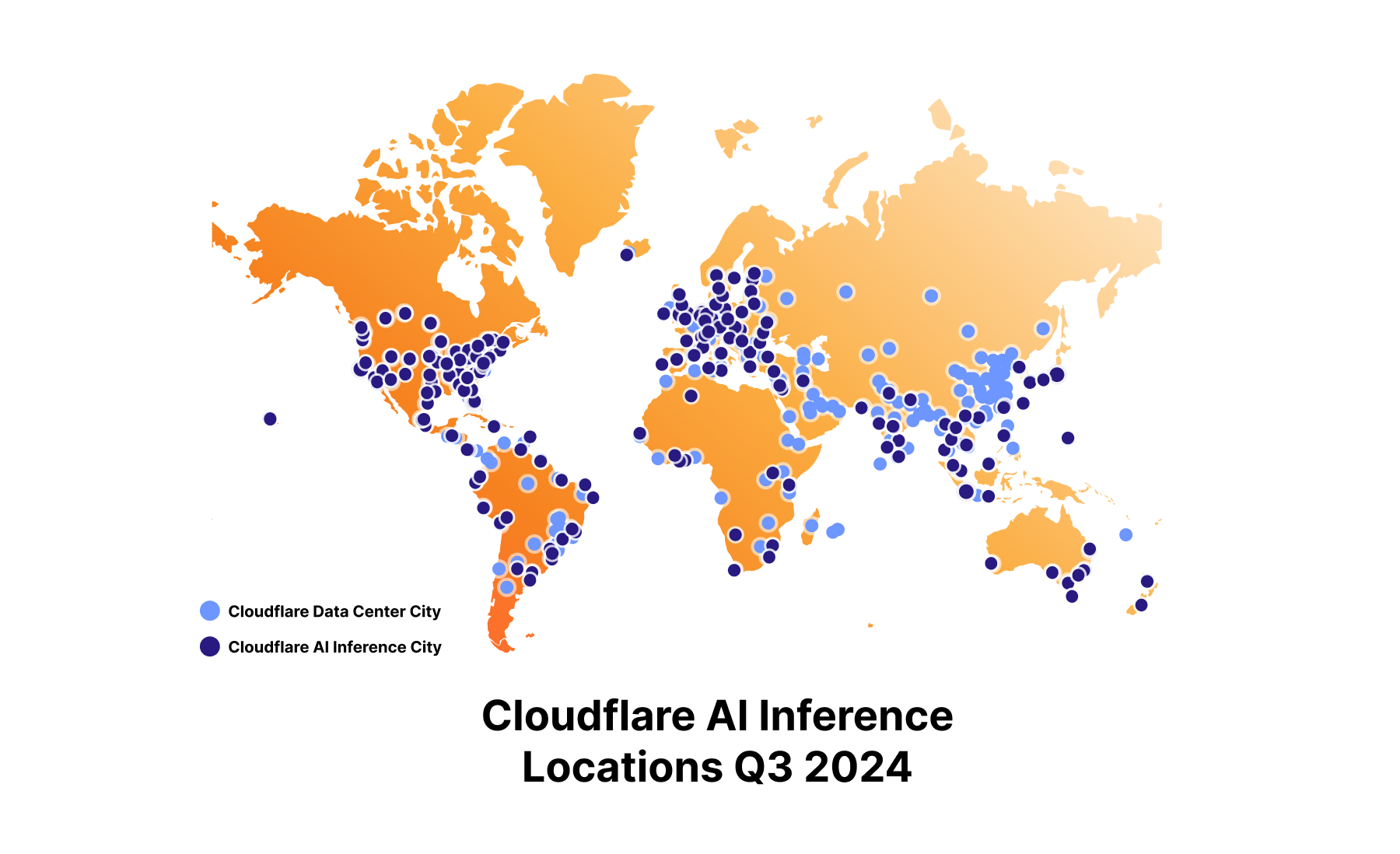
In addition to more powerful GPUs, we’ve continued to expand our GPU footprint to get as close to the user as possible, reducing latency even further. Today, we have GPUs in over 180 cities, having doubled our capacity in a year.
Bigger, better, faster
With the introduction of our new, more powerful GPUs, you can now run inference on significantly larger models, including Meta Llama 3.1 70B. Previously, our model catalog was limited to 8B parameter LLMs, but we can now support larger models, faster response times, and larger context windows. This means your applications can handle more complex tasks with greater efficiency.
Model
@cf/meta/Llama-3.2-11B-Vision-Instruct
@cf/meta/Llama-3.2-1B-Instruct
@cf/meta/Llama-3.2-3B-Instruct
@cf/meta/Llama-3.1-8B-Instruct
@cf/meta/Llama-3.1-70B-Instruct
@cf/black-forest-labs/flux-1-schnell
The set of models above are available on our new GPUs at faster speeds. If you’re using Llama 3.1, we’ve already upgraded you to the faster inference – so your applications are automatically sped up! In general, you can expect throughput of 80+ Tokens per Second (TPS) for 8b models and a Time To First Token of 300 ms (depending on where you are in the world).
Our model instances now support larger context windows, like the full 128K context window for Llama 3.1 and 3.2. To give you full visibility into performance, we’ll also be publishing metrics like TTFT, TPS, Context Window, and pricing on models in our catalog, so you know exactly what to expect.
We’re committed to bringing the best of open-source models to our platform, and that includes Meta’s release of the new Llama 3.2 collection of models. As a Meta launch partner, we were excited to have Day 0 support for the 11B vision model, as well as the 1B and 3B text-only model on Workers AI.
For more details on how we made Workers AI fast, take a look at our technical blog post, where we share a novel method for KV cache compression (it’s open-source!), as well as details on speculative decoding, our new hardware design, and more.
Greater model flexibility
With our commitment to helping you run more powerful models faster, we are also expanding the breadth of models you can run on Workers AI with our Run Any* Model feature. Until now, we have manually curated and added only the most popular open source models to Workers AI. Now, we are opening up our catalog to the public, giving you the flexibility to choose from a broader selection of models. We will support models that are compatible with our GPUs and inference stack at the start (hence the asterisk on Run Any* Model). We’re launching this feature in closed beta and if you’d like to try it out, please fill out the form, so we can grant you access to this new feature.
The Workers AI model catalog will now be split into two parts: a static catalog and a dynamic catalog. Models in the static catalog will remain curated by Cloudflare and will include the most popular open source models with guarantees on availability and speed (the models listed above). These models will always be kept warm in our network, ensuring you don’t experience cold starts. The usage and pricing model remains serverless, where you will only be charged for the requests to the model and not the cold start times.
Models that are launched via Run Any* Model will make up the dynamic catalog. If the model is public, users can share an instance of that model. In the future, we will allow users to launch private instances of models as well.
This is just the first step towards running your own custom or private models on Workers AI. While we have already been supporting private models for select customers, we are working on making this capacity available to everyone in the near future.
New Workers AI pricing
We launched Workers AI during Birthday Week 2023 with the concept of “neurons” for pricing. Neurons were intended to simplify the unit of measure across various models on our platform, including text, image, audio, and more. However, over the past year, we have listened to your feedback and heard that neurons were difficult to grasp and challenging to compare with other providers. Additionally, the industry has matured, and new pricing standards have materialized. As such, we’re excited to announce that we will be moving towards unit-based pricing and saying goodbye to neurons.
Moving forward, Workers AI will be priced based on model task, size, and units. LLMs will be priced based on the model size (parameters) and input/output tokens. Image generation models will be priced based on the output image resolution and the number of steps. Embeddings models will be priced based on input tokens. Speech-to-text models will be priced on seconds of audio input.
Model Task
Units
Model Size
Pricing
LLMs (incl. Vision models)
Tokens in/out (blended)
<= 3B parameters
$0.10 per Million Tokens
3.1B – 8B
$0.15 per Million Tokens
8.1B – 20B
$0.20 per Million Tokens
20.1B – 40B
$0.50 per Million Tokens
40.1B+
$0.75 per Million Tokens
Embeddings
Tokens in
<= 150M parameters
$0.008 per Million Tokens
151M+ parameters
$0.015 per Million Tokens
Speech-to-text
Audio seconds in
N/A
$0.0039 per minute of audio input
Image Size
Model Type
Steps
Price
<=256×256
Standard
25
$0.00125 per 25 steps
Fast
5
$0.00025 per 5 steps
<=512×512
Standard
25
$0.0025 per 25 steps
Fast
5
$0.0005 per 5 steps
<=1024×1024
Standard
25
$0.005 per 25 steps
Fast
5
$0.001 per 5 steps
<=2048×2048
Standard
25
$0.01 per 25 steps
Fast
5
$0.002 per 5 steps
We paused graduating models and announcing pricing for beta models over the past few months as we prepared for this new pricing change. We’ll be graduating all models to this new pricing, and billing will take effect on October 1, 2024.
Our free tier has been redone to fit these new metrics, and will include a monthly allotment of usage across all the task types.
Model
Free tier size
Text Generation – LLM
10,000 tokens a day across any model size
Embeddings
10,000 tokens a day across any model size
Images
Sum of 250 steps, up to 1024×1024 resolution
Whisper
10 minutes of audio a day
Optimizing AI workflows with AI Gateway
AI Gateway is designed to help developers and organizations building AI applications better monitor, control, and optimize their AI usage, and thanks to our users, AI Gateway has reached an incredible milestone — over 2 billion requests proxied by September 2024, less than a year after its inception. But we are not stopping there.
Persistent logs (open beta)
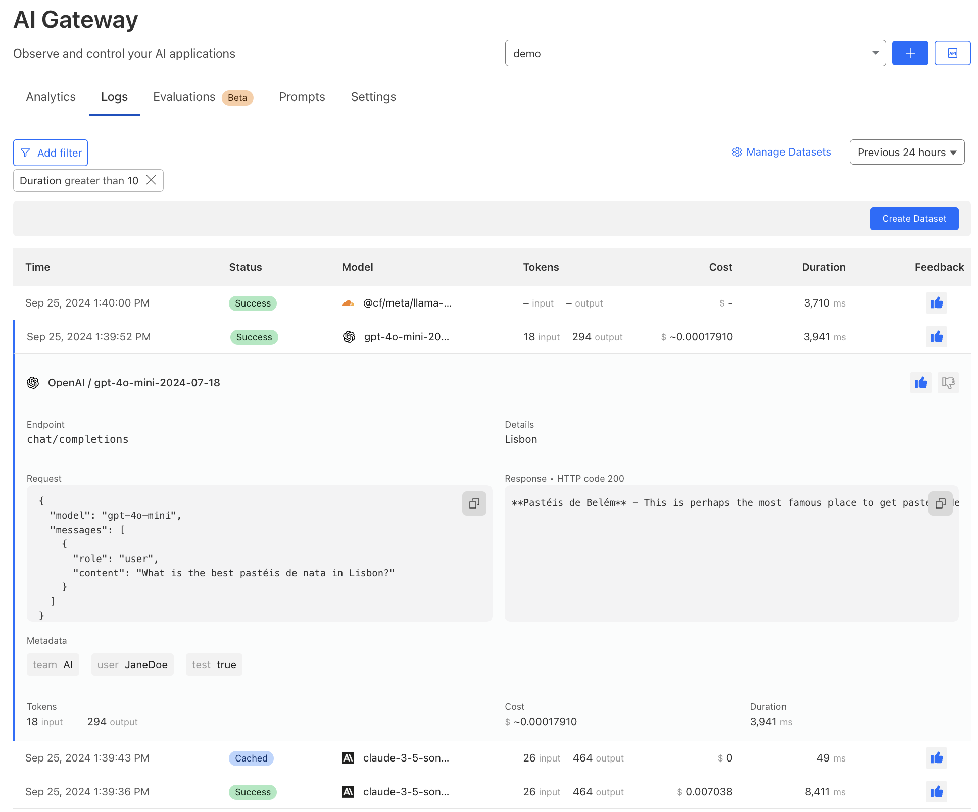
Persistent logs allow developers to store and analyze user prompts and model responses for extended periods, up to 10 million logs per gateway. Each request made through AI Gateway will create a log. With a log, you can see details of a request, including timestamp, request status, model, and provider.
We have revamped our logging interface to offer more detailed insights, including cost and duration. Users can now annotate logs with human feedback using thumbs up and thumbs down. Lastly, you can now filter, search, and tag logs with custom metadata to further streamline analysis directly within AI Gateway.
Persistent logs are available to use on all plans, with a free allocation for both free and paid plans. On the Workers Free plan, users can store up to 100,000 logs total across all gateways at no charge. For those needing more storage, upgrading to the Workers Paid plan will give you a higher free allocation — 200,000 logs stored total. Any additional logs beyond those limits will be available at $8 per 100,000 logs stored per month, giving you the flexibility to store logs for your preferred duration and do more with valuable data. Billing for this feature will be implemented when the feature reaches General Availability, and we’ll provide plenty of advance notice.
Workers Free
Workers Paid
Enterprise
Included Volume
100,000 logs stored (total)
200,000 logs stored (total)
Additional Logs
N/A
$8 per 100,000 logs stored per month
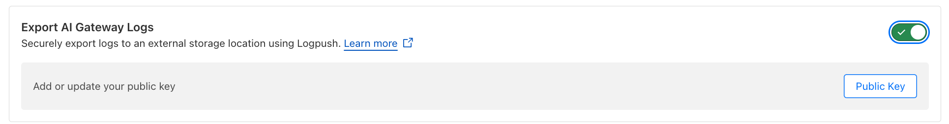
Export logs with Logpush
For users looking to export their logs, AI Gateway now supports log export via Logpush. With Logpush, you can automatically push logs out of AI Gateway into your preferred storage provider, including Cloudflare R2, Amazon S3, Google Cloud Storage, and more. This can be especially useful for compliance or advanced analysis outside the platform. Logpush follows its existing pricing model and will be available to all users on a paid plan.
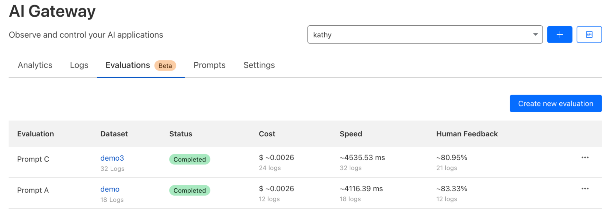
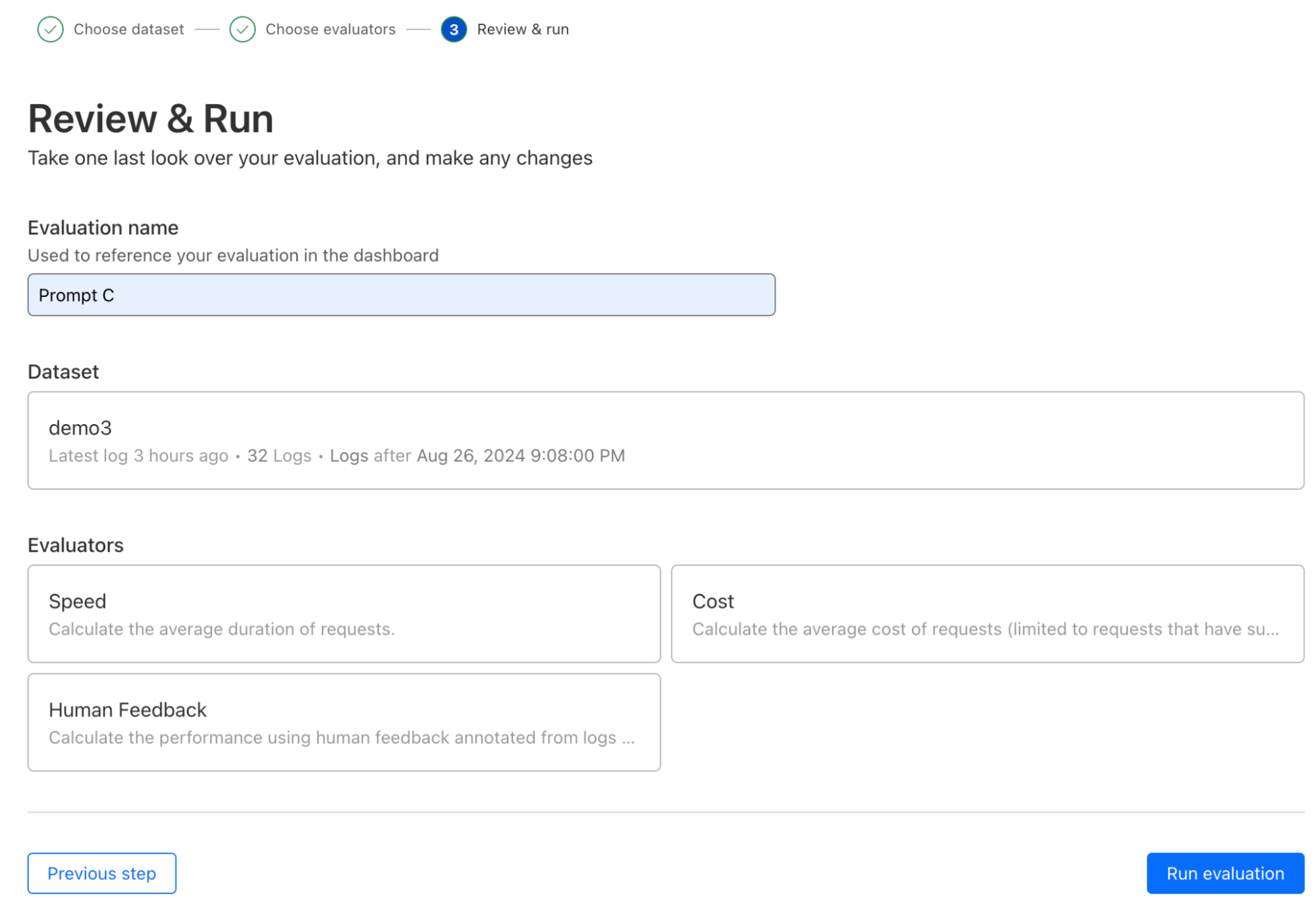
AI evaluations
We are also taking our first step towards comprehensive AI evaluations, starting with evaluation using human in the loop feedback (this is now in open beta). Users can create datasets from logs to score and evaluate model performance, speed, and cost, initially focused on LLMs. Evaluations will allow developers to gain a better understanding of how their application is performing, ensuring better accuracy, reliability, and customer satisfaction. We’ve added support for cost analysis across many new models and providers to enable developers to make informed decisions, including the ability to add custom costs. Future enhancements will include automated scoring using LLMs, comparing performance of multiple models, and prompt evaluations, helping developers make decisions on what is best for their use case and ensuring their applications are both efficient and cost-effective.
Vectorize GA
We’ve completely redesigned Vectorize since our initial announcement in 2023 to better serve customer needs. Vectorize (v2) now supports indexes of up to 5 million vectors (up from 200,000), delivers faster queries (median latency is down 95% from 500 ms to 30 ms), and returns up to 100 results per query (increased from 20). These improvements significantly enhance Vectorize’s capacity, speed, and depth of results.
Note: if you got started on Vectorize before GA, to ease the move from v1 to v2, a migration solution will be available in early Q4 — stay tuned!
New Vectorize pricing
Not only have we improved performance and scalability, but we’ve also made Vectorize one of the most cost-effective options on the market. We’ve reduced query prices by 75% and storage costs by 98%.
New Vectorize pricing
Old Vectorize pricing
Price reduction
Writes
Free
Free
n/a
Query
$.01 per 1 million vector dimensions
$0.04 per 1 million vector dimensions
75%
Storage
$0.05 per 100 million vector dimensions
$4.00 per 100 million vector dimensions
98%
You can learn more about our pricing in the Vectorize docs.
Vectorize free tier
There’s more good news: we’re introducing a free tier to Vectorize to make it easy to experiment with our full AI stack.
The free tier includes:
30 million queried vector dimensions / month
5 million stored vector dimensions / month
How fast is Vectorize?
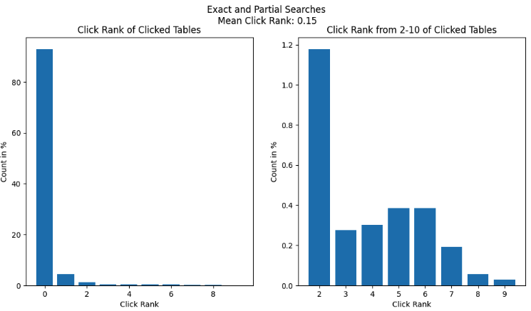
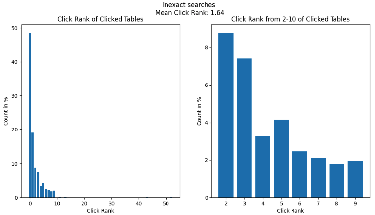
To measure performance, we conducted benchmarking tests by executing a large number of vector similarity queries as quickly as possible. We measured both request latency and result precision. In this context, precision refers to the proportion of query results that match the known true-closest results for all benchmarked queries. This approach allows us to assess both the speed and accuracy of our vector similarity search capabilities. Here are the following datasets we benchmarked on:
Laion-768-5m-ip: 5 million vectors, 768 dimensions, queried with cosine similarity at a top K of 10
We ran this again skipping the result-refinement pass to return approximate results faster
Benchmark dataset
P50 (ms)
P75 (ms)
P90 (ms)
P95 (ms)
Throughput (RPS)
Precision
dbpedia-openai-1M-1536-angular
31
56
159
380
343
95.4%
Laion-768-5m-ip
81.5
91.7
105
123
623
95.5%
Laion-768-5m-ip w/o refinement
14.7
19.3
24.3
27.3
698
78.9%
These benchmarks were conducted using a standard Vectorize v2 index, queried with a concurrency of 300 via a Cloudflare Worker binding. The reported latencies reflect those observed by the Worker binding querying the Vectorize index on warm caches, simulating the performance of an existing application with sustained usage.
Beyond Vectorize’s fast query speeds, we believe the combination of Vectorize and Workers AI offers an unbeatable solution for delivering optimal AI application experiences. By running Vectorize close to the source of inference and user interaction, rather than combining AI and vector database solutions across providers, we can significantly minimize end-to-end latency.
With these improvements, we’re excited to announce the general availability of the new Vectorize, which is more powerful, faster, and more cost-effective than ever before.
Tying it all together: the AI platform for all your inference needs
Over the past year, we’ve been committed to building powerful AI products that enable users to build on us. While we are making advancements on each of these individual products, our larger vision is to provide a seamless, integrated experience across our portfolio.
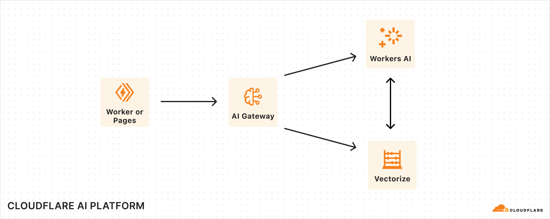
With Workers AI and AI Gateway, users can easily enable analytics, logging, caching, and rate limiting to their AI application by connecting to AI Gateway directly through a binding in the Workers AI request. We imagine a future where AI Gateway can not only help you create and save datasets to use for fine-tuning your own models with Workers AI, but also seamlessly redeploy them on the same platform. A great AI experience is not just about speed, but also accuracy. While Workers AI ensures fast performance, using it in combination with AI Gateway allows you to evaluate and optimize that performance by monitoring model accuracy and catching issues, like hallucinations or incorrect formats. With AI Gateway, users can test out whether switching to new models in the Workers AI model catalog will deliver more accurate performance and a better user experience.
In the future, we’ll also be working on tighter integrations between Vectorize and Workers AI, where you can automatically supply context or remember past conversations in an inference call. This cuts down on the orchestration needed to run a RAG application, where we can automatically help you make queries to vector databases.
If we put the three products together, we imagine a world where you can build AI apps with full observability (traces with AI Gateway) and see how the retrieval (Vectorize) and generation (Workers AI) components are working together, enabling you to diagnose issues and improve performance.
This Birthday Week, we’ve been focused on making sure our individual products are best-in-class, but we’re continuing to invest in building a holistic AI platform within our AI portfolio, but also with the larger Developer Platform Products. Our goal is to make sure that Cloudflare is the simplest, fastest, more powerful place for you to build full-stack AI experiences with all the batteries included.
We’re excited for you to try out all these new features! Take a look at our updated developer docs on how to get started and the Cloudflare dashboard to interact with your account.
Cloudflare is thrilled to announce the general deployment of our next generation of servers — Gen 12 powered by AMD EPYC 9684X (code name “Genoa-X”) processors. This next generation focuses on delivering exceptional performance across all Cloudflare services, enhanced support for AI/ML workloads, significant strides in power efficiency, and improved security features.
Here are some key performance indicators and feature improvements that this generation delivers as compared to the prior generation:
Beginning with performance, with close engineering collaboration between Cloudflare and AMD on optimization, Gen 12 servers can serve more than twice as many requests per second (RPS) as Gen 11 servers, resulting in lower Cloudflare infrastructure build-out costs.
Next, our power efficiency has improved significantly, by more than 60% in RPS per watt as compared to the prior generation. As Cloudflare continues to expand our infrastructure footprint, the improved efficiency helps reduce Cloudflare’s operational expenditure and carbon footprint as a percentage of our fleet size.
Third, in response to the growing demand for AI capabilities, we’ve updated the thermal-mechanical design of our Gen 12 server to support more powerful GPUs. This aligns with the Workers AI objective to support larger large language models and increase throughput for smaller models. This enhancement underscores our ongoing commitment to advancing AI inference capabilities
Fourth, to underscore our security-first position as a company, we’ve integrated hardware root of trust (HRoT) capabilities to ensure the integrity of boot firmware and board management controller firmware. Continuing to embrace open standards, the baseboard management and security controller (Data Center Secure Control Module or OCP DC-SCM) that we’ve designed into our systems is modular and vendor-agnostic, enabling a unified openBMC image, quicker prototyping, and allowing for reuse.
Finally, given the increasing importance of supply assurance and reliability in infrastructure deployments, our approach includes a robust multi-vendor strategy to mitigate supply chain risks, ensuring continuity and resiliency of our infrastructure deployment.
Cloudflare is dedicated to constantly improving our server fleet, empowering businesses worldwide with enhanced performance, efficiency, and security.
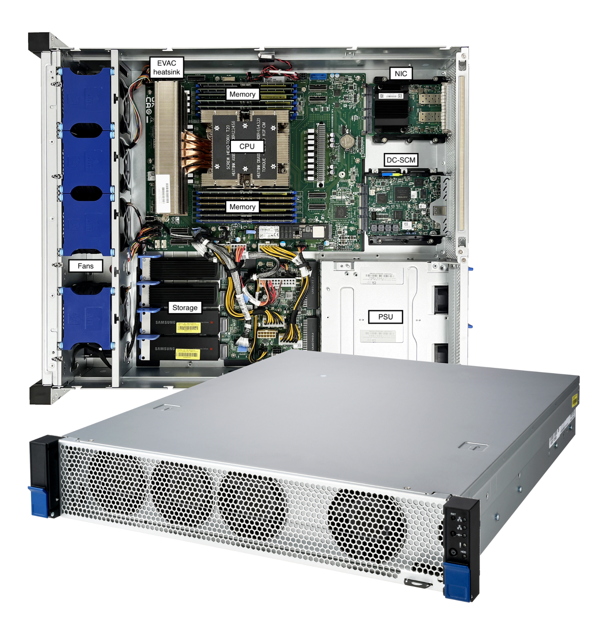
Gen 12 Servers
Let’s take a closer look at our Gen 12 server. The server is powered by a 4th generation AMD EPYC Processor, paired with 384 GB of DDR5 RAM, 16 TB of NVMe storage, a dual-port 25 GbE NIC, and two 800 watt power supply units.
During the design phase, we conducted an extensive survey of the CPU landscape. These options offer valuable choices as we consider how to shape the future of Cloudflare’s server technology to match the needs of our customers. We evaluated many candidates in the lab, and short-listed three standout CPU candidates from the 4th generation AMD EPYC Processor lineup: Genoa 9654, Bergamo 9754, and Genoa-X 9684X for production evaluation. The table below summarizes the differences in specifications of the short-listed candidates for Gen 12 servers against the AMD EPYC 7713 used in our Gen 11 servers. Notably, all three candidates offer significant increase in core count and marked increase in all core boost clock frequency.
*Note: AMD EPYC 7713 all core boost clock frequency of 2.7 GHz is not an official specification of the CPU but based on data collected at Cloudflare production fleet.
During production evaluation, the configuration of all three CPUs were optimized to the best of our knowledge, including thermal design power (TDP) configured to 400W for maximum performance. The servers are set up to run the same processes and services like any other server we have in production, which makes for a great side-by-side comparison.
Milan 7713
Genoa 9654
Bergamo 9754
Genoa-X 9684X
Production performance (request per second) multiplier
1x
2x
2.15x
2.45x
Production efficiency (request per second per watt) multiplier
1x
1.33x
1.38x
1.63x
AMD EPYC Genoa-X in Cloudflare Gen 12 server
Each of these CPUs outperforms the previous generation of processors by at least 2x. AMD EPYC 9684X Genoa-X with 3D V-cache technology gave us the greatest performance improvement, at 2.45x, when compared against our Gen 11 servers with AMD EPYC 7713 Milan.
Comparing the performance between Genoa-X 9684X and Genoa 9654, we see a ~22.5% performance delta. The primary difference between the two CPUs is the amount of L3 cache available on the CPU. Genoa-X 9684X has 1152 MB of L3 cache, which is three times the Genoa 9654 with 384 MB of L3 cache. Cloudflare workloads benefit from more low level cache being accessible and avoid the much larger latency penalty associated with fetching data from memory.
Genoa-X 9684X CPU delivered ~22.5% improved performance consuming the same amount of 400W power compared to Genoa 9654. The 3x larger L3 cache does consume additional power, but only at the expense of sacrificing 3% of highest achievable all core boost frequency on Genoa-X 9684X, a favorable trade-off for Cloudflare workloads.
More importantly, Genoa-X 9684X CPU delivered 145% performance improvement with only 50% system power increase, offering a 63% power efficiency improvement that will help drive down operational expenditure tremendously. It is important to note that even though a big portion of the power efficiency is due to the CPU, it needs to be paired with optimal thermal-mechanical design to realize the full benefit. Earlier last year, we made the thermal-mechanical design choice to double the height of the server chassis to optimize rack density and cooling efficiency across our global data centers. We estimated that moving from 1U to 2U would reduce fan power by 150W, which would decrease system power from 750 watts to 600 watts. Guess what? We were right — a Gen 12 server consumes 600 watts per system at a typical ambient temperature of 25°C.
While high performance often comes at a higher price, fortunately AMD EPYC 9684X offer an excellent balance between cost and capability. A server designed with this CPU provides top-tier performance without necessitating a huge financial outlay, resulting in a good Total Cost of Ownership improvement for Cloudflare.
Memory
AMD Genoa-X CPU supports twelve memory channels of DDR5 RAM up to 4800 mega transfers per second (MT/s) and per socket Memory Bandwidth of 460.8 GB/s. The twelve channels are fully utilized with 32 GB ECC 2Rx8 DDR5 RDIMM with one DIMM per channel configuration for a combined total memory capacity of 384 GB.
Choosing the optimal memory capacity is a balancing act, as maintaining an optimal memory-to-core ratio is important to make sure CPU capacity or memory capacity is not wasted. Some may remember that our Gen 11 servers with 64 core AMD EPYC 7713 CPUs are also configured with 384 GB of memory, which is about 6 GB per core. So why did we choose to configure our Gen 12 servers with 384 GB of memory when the core count is growing to 96 cores? Great question! A lot of memory optimization work has happened since we introduced Gen 11, including some that we blogged about, like Bot Management code optimization and our transition to highly efficient Pingora. In addition, each service has a memory allocation that is sized for optimal performance. The per-service memory allocation is programmed and monitored utilizing Linux control group resource management features. When sizing memory capacity for Gen 12, we consulted with the team who monitor resource allocation and surveyed memory utilization metrics collected from our fleet. The result of the analysis is that the optimal memory-to-core ratio is 4 GB per CPU core, or 384 GB total memory capacity. This configuration is validated in production. We chose dual rank memory modules over single rank memory modules because they have higher memory throughput, which improves server performance (read more about memory module organization and its effect on memory bandwidth).
The table below shows the result of running the Intel Memory Latency Checker (MLC) tool to measure peak memory bandwidth for the system and to compare memory throughput between 12 channels of dual-rank (2Rx8) 32 GB DIMM and 12 channels of single rank (1Rx4) 32 GB DIMM. Dual rank DIMMs have slightly higher (1.8%) read memory bandwidth, but noticeably higher write bandwidth. As write ratios increased from 25% to 50%, the memory throughput delta increased by 10%.
Benchmark
Dual rank advantage over single rank
Intel MLC ALL Reads
101.8%
Intel MLC 3:1 Reads-Writes
107.7%
Intel MLC 2:1 Reads-Writes
112.9%
Intel MLC 1:1 Reads-Writes
117.8%
Intel MLC Stream-triad like
108.6%
The table below shows the result of running the AMD STREAM benchmark to measure sustainable main memory bandwidth in MB/s and the corresponding computation rate for simple vector kernels. In all 4 types of vector kernels, dual rank DIMMs provide a noticeable advantage over single rank DIMMs.
Benchmark
Dual rank advantage over single rank
Stream Copy
115.44%
Stream Scale
111.22%
Stream Add
109.06%
Stream Triad
107.70%
Storage
Cloudflare’s Gen X server and Gen 11 server support M.2 form factor drives. We liked the M.2 form factor mainly because it was compact. The M.2 specification was introduced in 2012, but today, the connector system is dated and the industry has concerns about its ability to maintain signal integrity with the high speed signal specified by PCIe 5.0 and PCIe 6.0 specifications. The 8.25W thermal limit of the M.2 form factor also limits the number of flash dies that can be fitted, which limits the maximum supported capacity per drive. To address these concerns, the industry has introduced the E1.S specification and is transitioning from the M.2 form factor to the E1.S form factor.
In Gen 12, we are making the change to the EDSFF E1 form factor, more specifically the E1.S 15mm. E1.S 15mm, though still in a compact form factor, provides more space to fit more flash dies for larger capacity support. The form factor also has better cooling design to support more than 25W of sustained power.
While the AMD Genoa-X CPU supports 128 PCIe 5.0 lanes, we continue to use NVMe devices with PCIe Gen 4.0 x4 lanes, as PCIe Gen 4.0 throughput is sufficient to meet drive bandwidth requirements and keep server design costs optimal. The server is equipped with two 8 TB NVMe drives for a total of 16 TB available storage. We opted for two 8 TB drives instead of four 4 TB drives because the dual 8 TB configuration already provides sufficient I/O bandwidth for all Cloudflare workloads that run on each server.
Sequential Read (MB/s) :
6,700
Sequential Write (MB/s) :
4,000
Random Read IOPS:
1,000,000
Random Write IOPS:
200,000
Endurance
1 DWPD
PCIe GEN4 x4 lane throughput
7880 MB/s
Storage devices performance specification
Network
Cloudflare servers and top-of-rack (ToR) network equipment operate at 25 GbE speeds. In Gen 12, we utilized a DC-MHS motherboard-inspired design, and upgraded from an OCP 2.0 form factor to an OCP 3.0 form factor, which provides tool-less serviceability of the NIC. The OCP 3.0 form factor also occupies less space in the 2U server compared to PCIe-attached NICs, which improves airflow and frees up space for other application-specific PCIe cards, such as GPUs.
Cloudflare has been using the Mellanox CX4-Lx EN dual port 25 GbE NIC since our Gen 9 servers in 2018. Even though the NIC has served us well over the years, we are single sourced. During the pandemic, we were faced with supply constraints and extremely long lead times. The team scrambled to qualify the Broadcom M225P dual port 25 GbE NIC as our second-sourced NIC in 2022, ensuring we could continue to turn up servers to serve customer demand. With the lessons learned from single-sourcing the Gen 11 NIC, we are now dual-sourcing and have chosen the Intel Ethernet Network Adapter E810 and NVIDIA Mellanox ConnectX-6 Lx to support Gen 12. These two NICs are compliant with the OCP 3.0 specification and offer more MSI-X queues that can then be mapped to the increased core count on the AMD EPYC 9684X. The Intel Ethernet Network Adapter comes with an additional advantage, offering full Generic Segmentation Offload (GSO) support including VLAN-tagged encapsulated traffic, whereast many vendors either only support Partial GSO or do not support it at all today. With Full GSO support, the kernel spent noticeably less time in softirq segmenting packets, and servers with Intel E810 NICs are processing approximately 2% more requests per second.
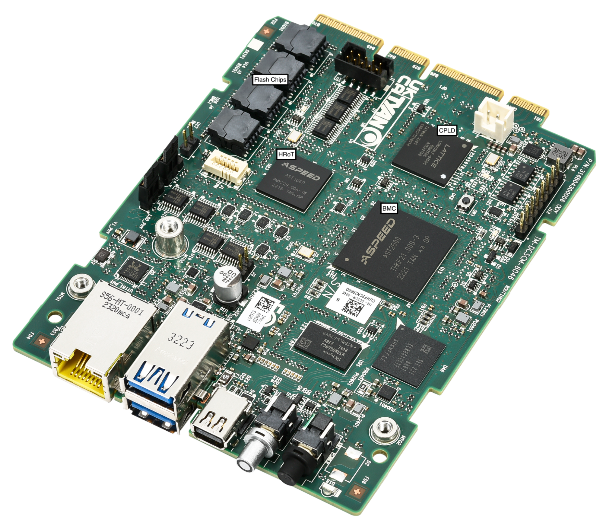
Improved security with DC-SCM: Project Argus
DC-SCM in Gen 12 server (Project Argus)
Gen 12 servers are integrated with Project Argus, one of the industry first implementations of Data Center Secure Control Module 2.0 (DC-SCM 2.0). DC-SCM 2.0 decouples server management and security functions away from the motherboard. The baseboard management controller (BMC), hardware root of trust (HRoT), trusted platform module (TPM), and dual BMC/BIOS flash chips are all installed on the DC-SCM.
On our Gen X and Gen 11 server, Cloudflare moved our secure boot trust anchor from the system Basic Input/Output System (BIOS) or the Unified Extensible Firmware Interface (UEFI) firmware to hardware-rooted boot integrity — AMD’s implementation of Platform Secure Boot (PSB) or Ampere’s implementation of Single Domain Secure Boot. These solutions helped secure Cloudflare infrastructure from BIOS / UEFI firmware attacks. However, we are still vulnerable to out-of-band attacks through compromising the BMC firmware. BMC is a microcontroller that provides out-of-band monitoring and management capabilities for the system. When compromised, attackers can read processor console logs accessible by BMC and control server power states for example. On Gen 12, the HRoT on the DC-SCM serves as the trust store of cryptographic keys and is responsible to authenticate the BIOS/UEFI firmware (independent of CPU vendor) and the BMC firmware for secure boot process.
In addition, on the DC-SCM, there are additional flash storage devices to enable storing back-up BIOS/UEFI firmware and BMC firmware to allow rapid recovery when a corrupted or malicious firmware is programmed, and to be resilient to flash chip failure due to aging.
These updates make our Gen 12 server more secure and more resilient to firmware attacks.
Power
A Gen 12 server consumes 600 watts at a typical ambient temperature of 25°C. Even though this is a 50% increase from the 400 watts consumed by the Gen 11 server, as mentioned above in the CPU section, this is a relatively small price to pay for a 145% increase in performance. We’ve paired the server up with dual 800W common redundant power supplies (CRPS) with 80 PLUS Titanium grade efficiency. Both power supply units (PSU) operate actively with distributed power and current. The units are hot-pluggable, allowing the server to operate with redundancy and maximize uptime.
80 PLUS is a PSU efficiency certification program. The Titanium grade efficiency PSU is 2% more efficient than the Platinum grade efficiency PSU between typical operating load of 25% to 50%. 2% may not sound like a lot, but considering the size of Cloudflare fleet with servers deployed worldwide, 2% savings over the lifetime of all Gen 12 deployment is a reduction of more than 7 GWh, equivalent to carbon sequestered by more than 3400 acres of U.S. forests in one year. This upgrade also means our Gen 12 server complies with EU Lot9 requirements and can be deployed in the EU region.
80 PLUS certification
10%
20%
50%
100%
80 PLUS Platinum
–
92%
94%
90%
80 PLUS Titanium
90%
94%
96%
91%
Drop-in GPU support
Demand for machine learning and AI workloads exploded in 2023, and Cloudflare introduced Workers AI to serve the needs of our customers. Cloudflare retrofitted or deployed GPUs worldwide in a portion of our Gen 11 server fleet to support the growth of Workers AI. Our Gen 12 server is also designed to accommodate the addition of more powerful GPUs. This gives Cloudflare the flexibility to support Workers AI in all regions of the world, and to strategically place GPUs in regions to reduce inference latency for our customers. With this design, the server can run Cloudflare’s full software stack. During times when GPUs see lower utilization, the server continues to serve general web requests and remains productive.
The electrical design of the motherboard is designed to support up to two PCIe add-in cards and the power distribution board is sized to support an additional 400W of power. The mechanics are sized to support either a single FHFL (full height, full length) double width GPU PCIe card, or two FHFL single width GPU PCIe cards. The thermal solution including the component placement, fans, and air duct design are sized to support adding GPUs with TDP up to 400W.
Looking to the future
Gen 12 Servers are currently deployed and live in multiple Cloudflare data centers worldwide, and already process millions of requests per second. Cloudflare’s EPYC journey has not ended — the 5th-gen AMD EPYC CPUs (code name “Turin”) are already available for testing, and we are very excited to start the architecture planning and design discussion for the Gen 13 server. Come join us at Cloudflare to help build a better Internet!
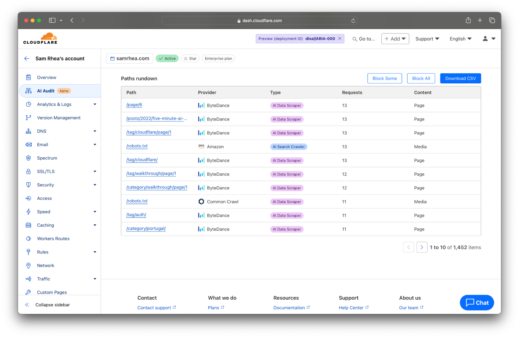
Site owners have lacked the ability to determine how AI services use their content for training or other purposes. Today, Cloudflare is releasing a set of tools to make it easy for site owners, creators, and publishers to take back control over how their content is made available to AI-related bots and crawlers. All Cloudflare customers can now audit and control how AI models access the content on their site.
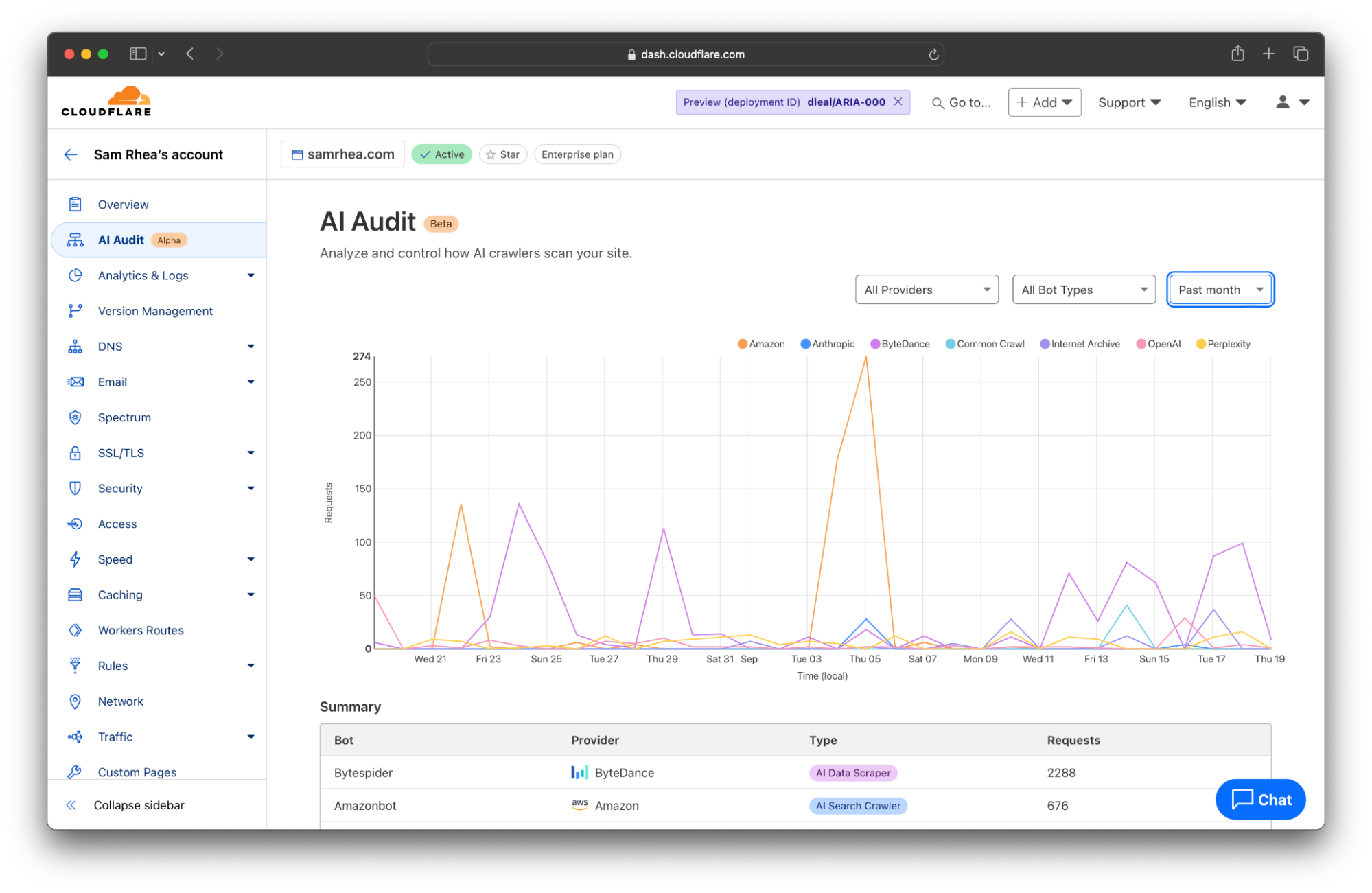
This launch starts with a detailed analytics view of the AI services that crawl your site and the specific content they access. Customers can review activity by AI provider, by type of bot, and which sections of their site are most popular. This data is available to every site on Cloudflare and does not require any configuration.
We expect that this new level of visibility will prompt teams to make a decision about their exposure to AI crawlers. To help give them time to make that decision, Cloudflare now provides a one-click option in our dashboard to immediately block any AI crawlers from accessing any site. Teams can then use this “pause” to decide if they want to allow specific AI providers or types of bots to proceed. Once that decision is made, those administrators can use new filters in the Cloudflare dashboard to enforce those policies in just a couple of clicks.
Some customers have already made decisions to negotiate deals directly with AI companies. Many of those contracts include terms about the frequency of scanning and the type of content that can be accessed. We want those publishers to have the tools to measure the implementation of these deals. As part of today’s announcement, Cloudflare customers can now generate a report with a single click that can be used to audit the activity allowed in these arrangements.
We also think that sites of any size should be able to determine how they want to be compensated for the usage of their content by AI models. Today’s announcement previews a new Cloudflare monetization feature which will give site owners the tools to set prices, control access, and capture value for the scanning of their content.
What is the problem?
Until recently, bots and scrapers on the Internet mostly fell into two clean categories: good and bad. Good bots, like search engine crawlers, helped audiences discover your site and drove traffic to you. Bad bots tried to take down your site, jump the queue ahead of your customers, or scrape competitive data. We built the Cloudflare Bot Management platform to give you the ability to distinguish between those two broad categories and to allow or block them.
The rise of AI Large Language Models (LLMs) and other generative tools created a murkier third category. Unlike malicious bots, the crawlers associated with these platforms are not actively trying to knock your site offline or to get in the way of your customers. They are not trying to steal sensitive data; they just want to scan what is already public on your site.
However, unlike helpful bots, these AI-related crawlers do not necessarily drive traffic to your site. AI Data Scraper bots scan the content on your site to train new LLMs. Your material is then put into a kind of blender, mixed up with other content, and used to answer questions from users without attribution or the need for users to visit your site. Another type of crawler, AI Search Crawler bots, scan your content and attempt to cite it when responding to a user’s search. The downside is that those users might just stay inside of that interface, rather than visit your site, because an answer is assembled on the page in front of them.
This murkiness leaves site owners with a hard decision to make. The value exchange is unclear. And site owners are at a disadvantage while they play catch up. Many sites allowed these AI crawlers to scan their content because these crawlers, for the most part, looked like “good” bots — only for the result to mean less traffic to their site as their content is repackaged in AI-written answers.
We believe this poses a risk to an open Internet. Without the ability to control scanning and realize value, site owners will be discouraged to launch or maintain Internet properties. Creators will stash more of their content behind paywalls and the largest publishers will strike direct deals. AI model providers will in turn struggle to find and access the long tail of high-quality content on smaller sites.
Both sides lack the tools to create a healthy, transparent exchange of permissions and value. Starting today, Cloudflare equips site owners with the services they need to begin fixing this. We have broken out a series of steps we recommend all of our customers follow to get started.
Step 1: Understand how AI models use your site
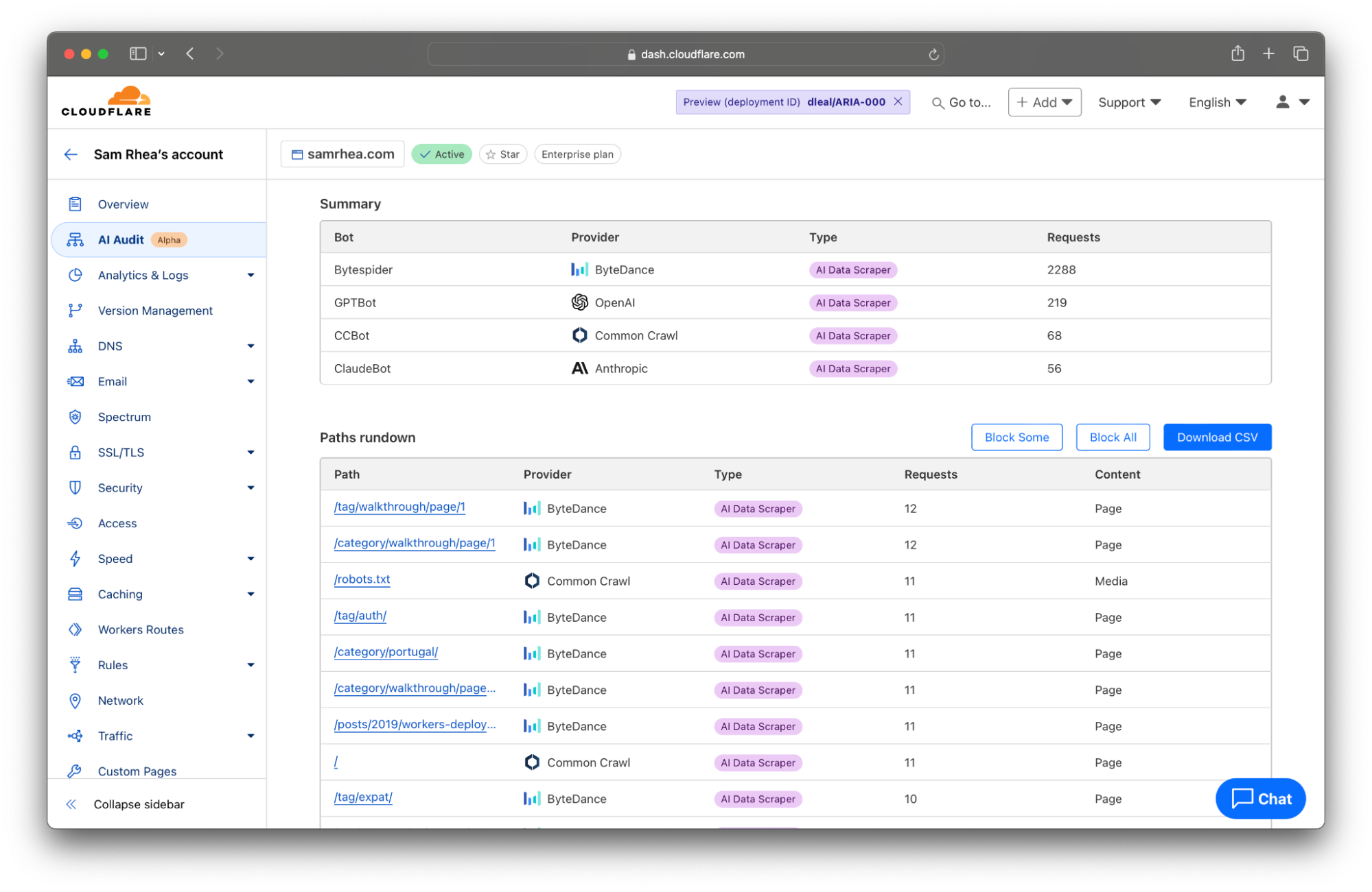
Every site on Cloudflare now has access to a new analytics view that summarizes the crawling behavior of popular and known AI services. You can begin reviewing this information to understand the AI scanning of your content by selecting a site in your dashboard and navigating to the AI Audit tab in the left-side navigation bar.
When AI model providers access content on your site, they rely on automated tools called “bots” or “crawlers” to scan pages. The bot will request the content of your page, capture the response, and store it as part of a future data training set or remember it for AI search engine results in the future.
These bots often identify themselves to your site (and Cloudflare’s network) by including an HTTP header in their request called a User Agent. Although, in some cases, a bot from one of these AI services might not send the header and Cloudflare instead relies on other heuristics like IP address or behavior to identify them.
When the bot does identify itself, the header will contain a string of text with the bot name. For example, Anthropic sometimes crawls sites on the Internet with a bot called ClaudeBot. When that service requests the content of a page from your site on Cloudflare, Cloudflare logs the User Agent as ClaudeBot.
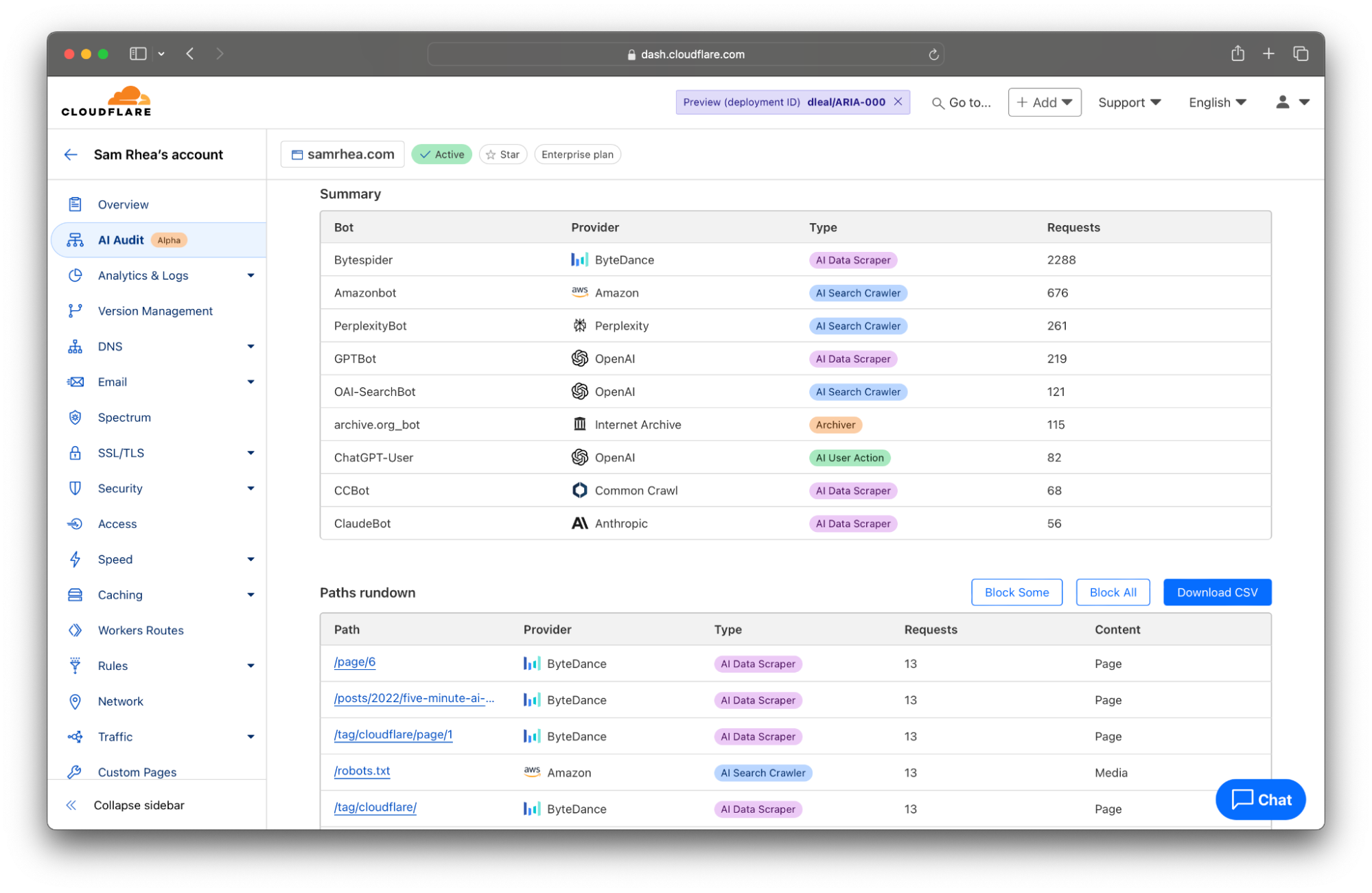
Cloudflare takes the logs gathered from visits to your site and looks for user agents that match known AI bots and crawlers. We summarize the activity of individual crawlers and also provide you with filters to review just the activities of specific AI platforms. Many AI firms rely on multiple crawlers that serve distinct purposes. When OpenAI scans sites for data scraping, they rely on GPTBot, but when they crawl sites for their new AI search engine, they use OAI-SearchBot.
And those differences matter. Scanning from different bot types can impact traffic to your site or the attribution of your content. AI search engines will often link to sites as part of their response, potentially sending visitors to your destination. In that case, you might be open to those types of bots crawling your Internet property. AI Data Scrapers, on the other hand, just exist to read as much of the Internet as possible to train future models or improve existing ones.
We think that you deserve to know why a bot is crawling your site in addition to when and how often. Today’s release gives you a filter to review bot activity by categories like AI Data Scraper, AI Search Crawler, and Archiver.
With this data, you can begin analyzing how AI models access your site. That information might be overwhelming, especially if your team has not had time yet to decide how you want to handle AI scanning of your content. If you find yourself unsure on how to respond, proceed to Step 2.
Step 2: Give yourself a pause to decide what to do next
We talked to several organizations who know their sites are valuable destinations for AI crawlers, but they do not yet know what to do about it. These teams need a “time out” so they can make an informed decision about how they make their data available to these services.
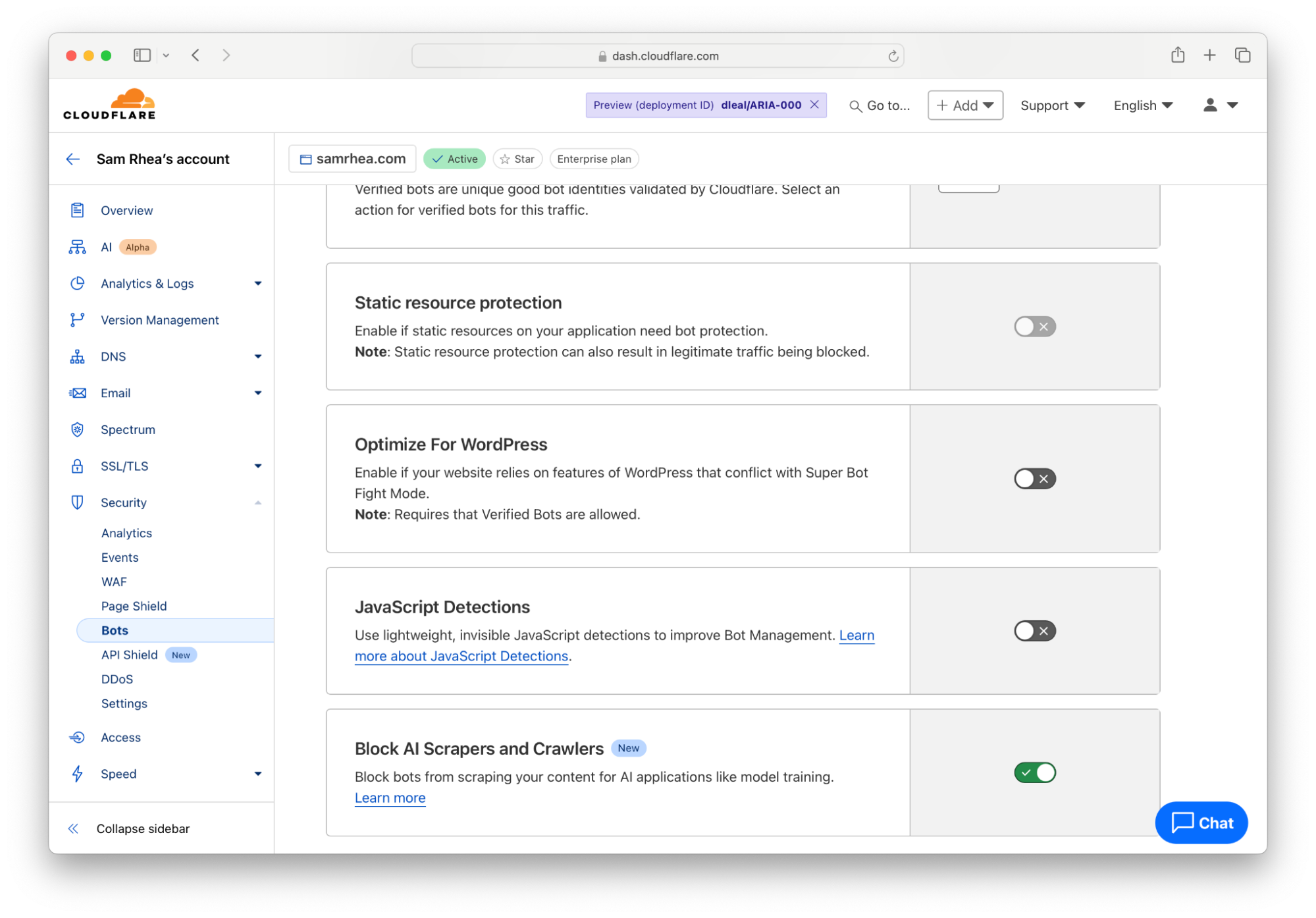
Cloudflare gives you that easy button right now. Any customer on any plan can choose to block all AI bots and crawlers to give yourself a pause while you decide what you do want to allow.
To implement that option, navigate to the Bots section under the Security tab of the Cloudflare Dashboard. Follow the blue link in the top right corner to configure how Cloudflare’s proxy handles bot traffic. Next, toggle the button in the “Block AI Scrapers and Crawlers” card to the “On” position.
The one-click option blocks known AI-related bots and crawlers from accessing your site based on a list that Cloudflare maintains. With a block in place, you and your team can make a less rushed decision about what to do next with your content.
Step 3: Control the bots you do want to allow
The pause button buys time for your team to decide what you want the relationship to be between these crawlers and your content. Once your team has reached a decision, you can begin relying on Cloudflare’s network to implement that policy.
If that decision is “we are not going to allow any crawling,” then you can leave the block button discussed above toggled to “On”. If you want to allow some selective scanning, today’s release provides you with options to permit certain types of bots, or just bots from certain providers, to access your content.
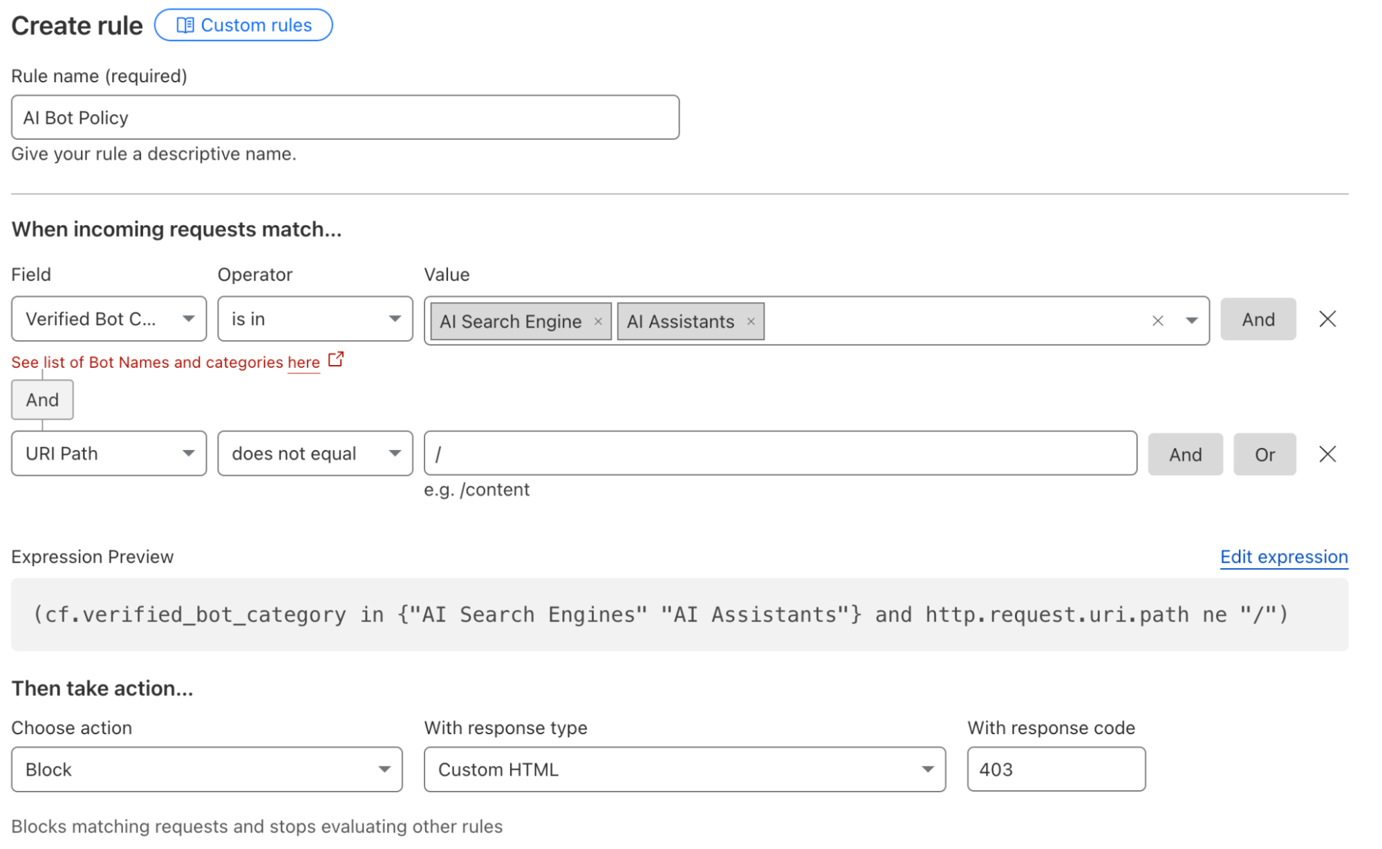
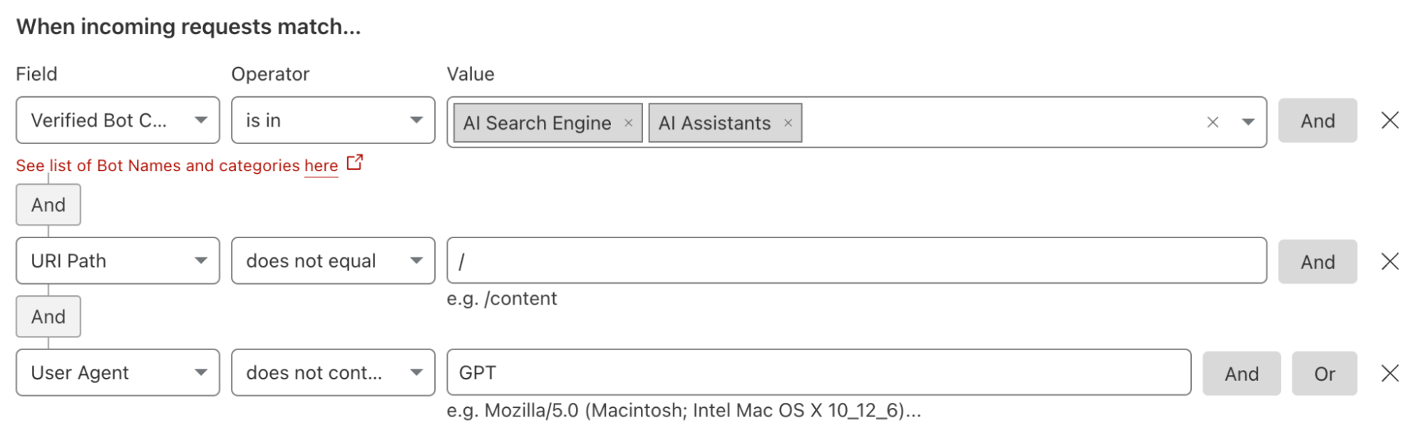
For some teams, the decision will be to allow the bots associated with AI search engines to scan their Internet properties because those tools can still drive traffic to the site. Other organizations might sign deals with a specific model provider, and they want to allow any type of bot from that provider to access their content. Customers can now navigate to the WAF section of the Cloudflare dashboard to implement these types of policies.
Administrators can also create rules that would, for example, block all AI bots except for those from a specific platform. Teams can deploy these types of filters if they are skeptical of most AI platforms but comfortable with one AI model provider and its policies. These types of rules can also be used to implement contracts where a site owner has negotiated to allow scanning from a single provider. The site administrator would need to create a rule to block all types of AI-related bots and then add an exception that allows the specific bot or bots from their AI partner.
We also recommend that customers consider updating their Terms of Service to cover this new use case in addition to applying these new filters. We have documented the steps we suggest that “good citizen” bots and crawlers take with respect to robots.txt files. As an extension of those best practices, we are adding a new section to that documentation where we provide a sample Terms of Service section that site owners can consider using to establish that AI scanning needs to follow the policies you have defined in your robots.txt file.
Step 4: Audit your existing scanning arrangements
An increasing number of sites are signing agreements directly with model providers to license consumption of their content in exchange for payment. Many of those deals contain provisions that determine the rate of crawling for certain sections or entire sites. Cloudflare’s AI Audit tab provides you with the tools to monitor those kinds of contracts.
The table at the bottom of the AI Audit tool now lists the most popular content on your site ranked by the count of scans in the time period from the filter set at the top of the page. You can click the Export to CSV button to quickly download a file with the details presented here that you can use to discuss any discrepancies with the AI platform that you are allowing to access your content.
Today, the data available to you represents key metrics we have heard from customers in these kinds of arrangements: requests against certain pages and requests against the entire site.
Step 5: Prepare your site to capture value from AI scanning
Not everyone has the time or contacts to negotiate deals with AI companies. Up to this point, only the largest publishers on the Internet have the resources to set those kinds of terms and get paid for their content.
Everyone else has been left with two basic choices on how to handle their data: block all scanning or allow unrestricted access. Today’s releases give content creators more visibility and control than just those two options, but the long tail of sites on the Internet still lack a pathway to monetization.
We think that sites of any size should be fairly compensated for the use of their content. Cloudflare plans to launch a new component of our dashboard that goes beyond just blocking and analyzing crawls. Site owners will have the ability to set a price for their site, or sections of their site, and to then charge model providers based on their scans and the price you have set. We’ll handle the rest so that you can focus on creating great content for your audience.
The fastest way to get ready to capture value through this new component is to make sure your sites use Cloudflare’s network. We plan to invite sites to participate in the beta based on the date they first joined Cloudflare. Interested in being notified when this is available? Let us know here.
Imagine a world where finding the right data is like searching for a needle in a haystack. In today’s data-driven landscape, companies are drowning in a sea of information, struggling to navigate through countless datasets to uncover valuable insights. At Grab, we faced a similar challenge. With over 200,000 tables in our data lake, along with numerous Kafka streams, production databases, and ML features, locating the most suitable dataset for our Grabber’s use cases promptly has historically been a significant hurdle.
Problem Space
Our internal data discovery tool, Hubble, built on top of the popular open-source platform Datahub, was primarily used as a reference tool. While it excelled at providing metadata for known datasets, it struggled with true data discovery due to its reliance on Elasticsearch, which performs well for keyword searches but cannot accept and use user-provided context (i.e., it can’t perform semantic search, at least in its vanilla form). The Elasticsearch parameters provided by Datahub out of the box also had limitations: our monthly average click-through rate was only 82%, meaning that in 18% of sessions, users abandoned their searches without clicking on any dataset. This suggested that the search results were not meeting their needs.
Another indispensable requirement for efficient data discovery that was missing at Grab was documentation. Documentation coverage for our data lake tables was low, with only 20% of the most frequently queried tables (colloquially referred to as P80 tables) having existing documentation. This made it difficult for users to understand the purpose and contents of different tables, even when browsing through them on the Hubble UI.
Consequently, data consumers heavily relied on tribal knowledge, often turning to their colleagues via Slack to find the datasets they needed. A survey conducted last year revealed that 51% of data consumers at Grab took multiple days to find the dataset they required, highlighting the inefficiencies in our data discovery process.
To address these challenges and align with Grab’s ongoing journey towards a data mesh architecture, the Hubble team recognised the importance of improving data discovery. We embarked on a journey to revolutionise the way our employees find and access the data they need, leveraging the power of AI and Large Language Models (LLMs).
Vision
Given the historical context, our vision was clear: to remove humans in the data discovery loop by automating the entire process using LLM-powered products. We aimed to reduce the time taken for data discovery from multiple days to mere seconds, eliminating the need for anyone to ask their colleagues data discovery questions ever again.
Goals
To achieve our vision, we set the following goals for ourselves for the first half of 2024:
Build HubbleIQ: An LLM-based chatbot that could serve as the equivalent of a Lead Data Analyst for data discovery. Just as a lead is an expert in their domain and can guide data consumers to the right dataset, we wanted HubbleIQ to do the same across all domains at Grab. We also wanted HubbleIQ to be accessible where data consumers hang out the most: Slack.
Improve documentation coverage: A new Lead Analyst joining the team would require extensive documentation coverage of very high quality. Without this, they wouldn’t know what data exists and where. Thus, it was important for us to improve documentation coverage.
Enhance Elasticsearch: We aimed to tune our Elasticsearch implementation to better meet the requirements of Grab’s data consumers.
A Systematic Path to Success
Step 1: Enhance Elasticsearch
Through clickstream analysis and user interviews, the Hubble team identified four categories of data search queries that were seen either on the Hubble UI or in Slack channels:
Exact search: Queries belonging to this category were a substring of an existing dataset’s name at Grab, with the query length being at least 40% of the dataset’s name.
Partial search: The Levenshtein distance between a query in this category and any existing dataset’s name was greater than 80. This category usually comprised queries that closely resembled an existing dataset name but likely contained spelling mistakes or were shorter than the actual name.
Exact and partial searches accounted for 75% of searches on Hubble (and were non-existent on Slack: as a human, receiving a message that just had the name of a dataset would feel rather odd). Given the effectiveness of vanilla Elasticsearch for these categories, the click rank was close to 0.
Inexact search: This category comprised queries that were usually colloquial keywords or phrases that may be semantically related to a given table, column, or piece of documentation (e.g., “city” or “taxi type”). Inexact searches accounted for the remaining 25% of searches on Hubble. Vanilla Elasticsearch did not perform well in this category since it relied on pure keyword matching and did not consider any additional context.
Semantic search: These were free text queries with abundant contextual information supplied by the user. Hubble did not see any such queries as users rightly expected that Hubble would not be able to fulfil their search needs. Instead, these queries were sent by data consumers to data producers via Slack. Such queries were numerous, but usually resulted in data hunting journeys that spanned multiple days – the root of frustration amongst data consumers.
The first two search types can be seen as “reference” queries, where the data consumer already knows what they are looking for. Inexact and contextual searches are considered “discovery” queries. The Hubble team noticed drop-offs in inexact searches because users learned that Hubble could not fulfil their discovery needs, forcing them to search for alternatives.
Through user interviews, the team discovered how Elasticsearch should be tuned to better fit the Grab context. They implemented the following optimisations:
Tagging and boosting P80 tables
Boosting the most relevant schemas
Hiding irrelevant datasets like PowerBI dataset tables
Deboosting deprecated tables
Improving the search UI by simplifying and reducing clutter
Adding relevant tags
Boosting certified tables
As a result of these enhancements, the click-through rate rose steadily over the course of the half to 94%, a 12 percentage point increase.
While this helped us make significant improvements to the first three search categories, we knew we had to build HubbleIQ to truly automate the last category – semantic search.
Step 2: Build a Context Store for HubbleIQ
To support HubbleIQ, we built a documentation generation engine that used GPT-4 to generate documentation based on table schemas and sample data. We refined the prompt through multiple iterations of feedback from data producers.
We added a “generate” button on the Hubble UI, allowing data producers to easily generate documentation for their tables. This feature also supported the ongoing Grab-wide initiative to certify tables.
In conjunction, we took the initiative to pre-populate docs for the most critical tables, while notifying data producers to review the generated documentation. Such docs were visible to data consumers with an “AI-generated” tag as a precaution. When data producers accepted or edited the documentation, the tag was removed.
As a result, documentation coverage for P80 tables increased by 70 percentage points to ~90%. User feedback showed that ~95% of users found the generated docs useful.
Step 3: Build and Launch HubbleIQ
With high documentation coverage in place, we were ready to harness the power of LLMs for data discovery. To speed up go-to-market, we decided to leverage Glean, an enterprise search tool used by Grab.
First, we integrated Hubble with Glean, making all data lake tables with documentation available on the Glean platform. Next, we used Glean Apps to create the HubbleIQ bot, which was essentially an LLM with a custom system prompt that could access all Hubble datasets that were catalogued on Glean. Finally, we integrated this bot into Hubble search, such that for any search that is likely to be a semantic search, HubbleIQ results are shown on top, followed by regular search results.
Recently, we integrated HubbleIQ with Slack, allowing data consumers to discover datasets without breaking their flow. Currently, we are working with analytics teams to add the bot to their “ask” channels (where data consumers come to ask contextual search queries for their domains). After integration, HubbleIQ will act as the first line of defence for answering questions in these channels, reducing the need for human intervention.
The impact of these improvements was significant. A follow-up survey revealed that 73% of respondents found it easy to discover datasets, marking a substantial 17 percentage point increase from the previous survey. Moreover, Hubble reached an all-time high in monthly active users, demonstrating the effectiveness of the enhancements made to the platform.
Next Steps
We’ve made significant progress towards our vision, but there’s still work to be done. Looking ahead, we have several exciting initiatives planned to further enhance data discovery at Grab.
On the documentation generation front, we aim to enrich the generator with more context, enabling it to produce even more accurate and relevant documentation. We also plan to streamline the process by allowing analysts to auto-update data docs based on Slack threads directly from Slack. To ensure the highest quality of documentation, we will develop an evaluator model that leverages LLMs to assess the quality of both human and AI-written docs. Additionally, we will implement Reflexion, an agentic workflow that utilises the outputs from the doc evaluator to iteratively regenerate docs until a quality benchmark is met or a maximum try-limit is reached.
As for HubbleIQ, our focus will be on continuous improvement. We’ve already added support for metric datasets and are actively working on incorporating other types of datasets as well. To provide a more seamless user experience, we will enable users to ask follow-up questions to HubbleIQ directly on the HubbleUI, with the system intelligently pulling additional metadata when a user mentions a specific dataset.
Conclusion
By harnessing the power of AI and LLMs, the Hubble team has made significant strides in improving documentation coverage, enhancing search capabilities, and drastically reducing the time taken for data discovery. While our efforts so far have been successful, there are still steps to be taken before we fully achieve our vision of completely replacing the reliance on data producers for data discovery. Nonetheless, with our upcoming initiatives and the groundwork we have laid, we are confident that we will continue to make substantial progress in the right direction over the next few production cycles.
As we forge ahead, we remain dedicated to refining and expanding our AI-powered data discovery tools, ensuring that Grabbers have every dataset they need to drive Grab’s success at their fingertips. The future of data discovery at Grab is brimming with possibilities, and the Hubble team is thrilled to be at the forefront of this exciting journey.
To our readers, we hope that our journey has inspired you to explore how you can leverage the power of AI to transform data discovery within your own organisations. The challenges you face may be unique, but the principles and strategies we have shared can serve as a foundation for your own data discovery revolution. By embracing innovation, focusing on user needs, and harnessing the potential of cutting-edge technologies, you too can unlock the full potential of your data and propel your organisation to new heights. The future of data-driven innovation is here, and we invite you to join us on this exhilarating journey.
Join us
Grab is the leading superapp platform in Southeast Asia, providing everyday services that matter to consumers. More than just a ride-hailing and food delivery app, Grab offers a wide range of on-demand services in the region, including mobility, food, package and grocery delivery services, mobile payments, and financial services across 700 cities in eight countries.
Powered by technology and driven by heart, our mission is to drive Southeast Asia forward by creating economic empowerment for everyone. If this mission speaks to you, join our team today!
Generative artificial intelligence (AI) is now a household topic and popular across various public applications. Users enter prompts to get answers to questions, write code, create images, improve their writing, and synthesize information. As people become familiar with generative AI, businesses are looking for ways to apply these concepts to their enterprise use cases in a simple, scalable, and cost-effective way. These same needs are shared by a variety of security stakeholders. For example, if security directors want to summarize their security posture in natural language, a security architect will need to triage alerts or findings and investigate AWS CloudTrail logs to identify high priority remediation actions or detect potential threat actors by identifying potentially malicious activity. There are many ways to deploy solutions for these use cases.
In this blog post, we review a fully serverless solution for querying data stored in Amazon Security Lake using natural language (human language) with Amazon Q in QuickSight. This solution has multiple use cases, such as generating visualizations and querying vulnerability information for vulnerability management using tools such as Amazon Inspector that feed into AWS Security Hub. The solution helps reduce the time from detection to investigation by using natural language to query CloudTrail logs and Amazon Virtual Private Cloud (VPC) Flow Logs, resulting in quicker response to threats in your environment.
Amazon Security Lake is a fully managed security data lake service that automatically centralizes security data from AWS environments, software as a service (SaaS) providers, and on-premises and cloud sources into a purpose-built data lake that’s stored in your AWS account. The data lake is backed by Amazon Simple Storage Service (Amazon S3) buckets, and you retain ownership over your data. Security Lake converts ingested data into Apache Parquet format and a standard open source schema called the Open Cybersecurity Schema Framework (OCSF). With OCSF support, Security Lake normalizes and combines security data from AWS and a broad range of enterprise security data sources.
Amazon QuickSight is a cloud-scale business intelligence (BI) service that delivers insights to stakeholders, wherever they are. QuickSight connects to your data in the cloud and combines data from a variety of different sources. With QuickSight, users can meet varying analytic needs from the same source of truth through interactive dashboards, reports, natural language queries, and embedded analytics. With Amazon Q in QuickSight, business analysts and users can use natural language to build, discover, and share meaningful insights.
The recent announcements for Amazon Q in QuickSight, Security Lake, and the OCSF present a unique opportunity to apply generative AI to fully managed hybrid multi-cloud security related logs and findings from over 100 independent software vendors and partners.
Solution overview
The solution uses Security Lake as the data lake which has native ingestion for CloudTrail, VPC Flow Logs, and Security Hub findings as shown in Figure 1. Logs from these sources are sent to S3 buckets in your AWS account and are maintained by Security Lake. We then create Amazon Athena views from tables created by Security Lake for Security Hub findings, CloudTrail logs, and VPC Flow Logs to define the interesting fields from each of the log sources. Each of these views are ingested into a QuickSight dataset. From these datasets, we generate analyses and dashboards. We use Amazon Q topics to label columns in the dataset that are human-readable and create a named entity to present contextual and multi-visual answers in response to questions. After the topics are created, users can perform their analysis using Q topics, QuickSight analyses, or QuickSight dashboards.
Figure 1: Solution architecture
You can use the rollup AWS Region feature in Security Lake to aggregate logs from multiple Regions into a single Region. Specifying a rollup Region can help you adhere to regional compliance requirements. If you use rollup Regions, you must set up the solution described in this post for datasets only in rollup Regions. If you don’t use a rollup Region, you must deploy this solution for each Region you that want to collect data from.
Prerequisites
To implement the solution described in this post, you must meet the following requirements:
Basic understanding of Security Lake, Athena, and QuickSight.
Security Lake is already deployed and accepting CloudTrail management events, VPC Flow Logs, and Security Hub findings as sources. If you haven’t deployed Security Lake yet, we recommend following the best practices established in the security reference architecture.
This solution uses Security Lake data source version 2 to create the dashboards and visualizations. If you aren’t already using data source version 2, you will see a banner in your Security Lake console with instructions to update.
An existing QuickSight deployment that will be used to visualize Security Lake data or an account that is able to sign up for QuickSight to create visualizations.
QuickSight Author Pro and Reader Pro licenses are needed for using Amazon Q features in QuickSight. Non-pro Authors and Readers can still access Q topics if an Author Pro or Admin Pro user shares the topic with them. Non-pro Authors and Readers can also access data stories if a Reader Pro, Author Pro, or Admin Pro shares one with them. Review Generative AI features supported by each QuickSight licensing tiers.
In the following section, we walk through the steps to ingest Security Lake data into QuickSight using Athena views and then using Amazon Q in QuickSight to create visualizations and query data using natural language.
Provide cross-account query access
In alignment with our security reference architecture, it’s a best practice to isolate the Security Lake account from the accounts that are running the visualization and querying workloads. It’s recommended that QuickSight for security use cases be deployed in the security tooling account. See How to visualize Amazon Security Lake findings with Amazon QuickSight for information on how to set up cross-account query access. Follow the steps in the Configure a Security Lake subscriber section and configure Athena to visualize your data section.
When you get to the create resource link steps, create a resource link for data source version 2 for Security Hub, CloudTrail, and VPC flow log tables for a total of three resource links. The way to identify data source version 2 tables is by their name; it ends in _2_0. For example:
For the remainder of this post, we will be referencing the database name security_lake_visualization and the resource link names for Security Hub findings, CloudTrail logs, and VPC Flow Logs respectively, as shown in Figure 2:
We will call the QuickSight account the visualization account. If you plan to use same account as the Security Lake delegated administrator and QuickSight, then skip this step and go to the next section where you will create views in Athena.
Create views in Athena
A view in Athena is a logical table that helps simplify your queries by working with only a subset of the relevant data. Follow these steps to create three views in Athena, one each for Security Hub findings, CloudTrail logs, and the VPC Flow Logs in the visualization account.
These queries default to the previous week’s data starting from the previous day, but you can change the time frame by modifying the last line in the query from 8 to the number of days you prefer. Keep in mind that there is a limitation on the size of each SPICE table of 1 TB. If you want to limit the volume of data, you can delete the rows that you find unnecessary. We included the fields customers have identified as relevant to reduce the burden of writing the parsing details yourself.
To create views:
Sign in to the AWS Management Console in the visualization account and navigate to the Athena console.
If a Security Lake rollup Region is used, select the rollup Region.
Choose Launch Query Editor.
If this is the first time you’re using Athena, you will need to choose a bucket to store your query results.
Choose Edit Settings.
Choose Browse S3.
Search for your bucket name.
Select the radio button next to the name of your bucket.
Select Choose.
For Data Source, select AWSDataCatalog.
Select Database as security_lake_visualization. If you used a different name for the database for cross account query access, then select that database.
Figure 3: Athena database selection
Copy the query for the security_hub_view from the GitHub repo for this post. If you’re using a different name for the database and table resource link than the one specified in this post, edit the FROM statement at the bottom of the query to reflect the correct names.
Paste the query in the query editor and then choose Run. The name of the view is set in the first line of the query which is security_insights_security_hub_vw2.
To confirm this view was created correctly, choose the three dots next to the view that was created and select Preview View.
Figure 4: Previewing the view
Repeat steps 5–9 to create the CloudTrail and VPC Flow Logs views. The queries for each can be found in the GitHub repo.
Figure 5: Athena views
Create QuickSight dataset
Now that you’ve created the views, use Athena as the data source to create a dataset in QuickSight. Repeat these steps for the Security Hub findings, CloudTrail logs, and VPC Flow Logs. Start by creating a dataset for the Security Hub findings.
To configure permissions on tables:
Sign in to the QuickSight console in the visualization account. If a Security Lake rollup Region is used, select the rollup Region.
Although there are multiple ways to sign in to QuickSight, we used IAM based access to build the dashboards. To use QuickSight with Athena and Lake Formation, you first need to authorize connections through Lake Formation.
When using a cross-account configuration with AWS Glue Data Catalog, you need to configure permissions on tables that are shared through Lake Formation. For the use case in this post, use the following steps to grant access on the cross-account tables in the Glue Catalog. You must perform these steps for each of the Security Hub, CloudTrail, and VPC Flow Logs tables that you created in the preceding cross-account query access section. Because granting permissions on a resource link doesn’t grant permissions on the target (linked) database or table, you will grant permission twice, once to the target (linked table) and then to the resource link.
In the Lake Formation console, navigate to the Tables section and select the resource link for the Security Hub table. For example:
Select Actions. Under Permissions, select Grant on target.
For the next step, you need the Amazon Resource Name (ARN) of the QuickSight users or groups that need access to the table. To obtain the ARN through the AWS Command Line Interface (AWS CLI), run following commands (replacing account ID and Region with that of the visualization account.) You can use AWS CloudShell for this purpose.
After you have the ARN of the user or group, copy it and go back to the LakeFormation console Grant on Target page. For Principals, select SAML users and groups, and then add the QuickSight user’s ARN.
Figure 6: Selecting principals
For LF-Tags or catalog resources, keep the default settings.
Figure 7: Table grant on target permissions
For Table permissions, select Select for both Table Permissions and Grantable Permissions, and then choose Grant.
Figure 8: Selecting table permissions
Navigate back to the Tables section and select the resource link for the Security Hub table. For example:
Select Actions. This time under Permissions, and then choose Grant.
For Principals, select SAML users and groups, and then add the QuickSight user’s ARN captured earlier.
For the LF-Tags or catalog resources section, use the default settings.
For Resource link permissions choose Describe for both Table Permissions and Grantable Permissions.
Repeat steps a–k for the CloudTrail and VPC Flow Logs resource links.
To create datasets from views:
After permissions are in place, you create three datasets from the views created earlier. Because both Quicksight and Lake Formation are Regional services, verify that you’re using QuickSight in the same Region where Lake Formation is sharing the data. The simplest way to determine your Region is to check the QuickSight URL in your web browser. The Region will be at the beginning of the URL, such as us-east-1. To change the Region, select the settings icon in the top right of the QuickSight screen and select the correct Region from the list of available Regions in the drop-down menu.
Navigate back to the QuickSight console.
Select Datasets, and then choose New dataset.
Select Athena from the list of available data sources.
Enter a Data source name, for example security_lake_securityhub_dataset and leave the Athena workgroup as [primary]. Choose Create data source.
At the Choose your table prompt, for Catalog, select AwsDataCatalog. For Database, select security_lake_visualization. If you used a different name for the database for cross-account query access, then select that database. For Tables, select the view name security_insights_security_hub_vw2 to build your dashboards for Security Hub findings. Then choose Select.
Figure 9: Choose a table during QuickSight dataset creation
At the Finish dataset creation prompt, select Import to SPICE for quicker analytics. Choose Visualize. This will create a new dataset in QuickSight using the name of the Athena view, which is security_insights_security_hub_vw2. You will be taken to the Analysis page, exit out of it.
Go back to the QuickSight console and repeat steps 3–8 for the CloudTrail and VPC Flow Log datasets.
Create a topic
Now that you have created a dataset, you can create a topic. Q topics are collections of one or more datasets that represent a subject area for your business users to ask questions. Topics allow users to ask questions in natural language and to build visualizations using natural language.
To create a Q topic:
Navigate to the QuickSight console.
Choose Topics in the left navigation pane.
Figure 10: QuickSight navigation pane
Choose New topic. Create one topic each for the Security Hub findings, CloudTrail logs, and VPC Flow Logs
Figure 11: QuickSight topic creation
On the New topic page, do the following:
For Topic name, enter a descriptive name for the topic. Name the first one SecurityHubTopic. Your business users will identify the topic by this name and use it to ask questions.
For Description, enter a description for the topic. Your users can use this description to get more details about the topic.
Choose Continue.
On the Add data to topic page, choose the dataset you created in the Create a QuickSight dataset section. Start with the Security Hub dataset security_insights_security_hub_vw2.
Choose Continue. It will take a few minutes to create the topic.
Now that your topic has been created, navigate to the Data tab of the topic.
Your Data Fields sub-tab should be selected already. If not, choose Data Fields.
Figure 12: Topics data fields
For each of the fields in the list, turn on Include to make sure that all fields are included. For this example, we selected all fields, but you can adjust the included columns as needed for your use case. Note, you might see a banner at the top of the page indicating that the indexing is in progress. Depending on the size of your data, it might take some time for Q to make those fields available for querying. Most of the time, indexing is complete in less than 15 minutes.
Review the Synonyms column. These alternate representations of your column name are automatically generated by Amazon Q. You can add and remove synonyms as needed for your use case.
At this point, you’re ready to ask questions about your data using Amazon Q in QuickSight. Choose Ask a question about SecurityHubTopic at the top of the page.
Figure 13: Ask questions using Q
You can now ask questions about Security Hub findings in the prompt. Enter Show me findings with compliance status failed along with control id.
Figure 14: Q answers
Under the question, you will see how it was interpreted by QuickSight.
Repeat steps 1–13 to create CloudTrail and VPC Flow Log QuickSight topics.
Create named entities for your topics
Now that you’ve created your topics, you will now add named entities. Named entities are optional, but we’re using them in the solution to help make queries more effective. The information contained in named entities, the ordering of fields, and their ranking make it possible to present contextual, multi-visual answers in response to even vague questions.
To create a named entity:
In the QuickSight console, navigate to Topics.
Select the Security Hub topic that you created in the previous section.
Under the Data tab, select the Named Entity subtab, and choose Add Named Entity.
Figure 15: Named entity subtab
Enter Security Findings as the entity name.
Select the following datafields: Status, Metadata Product Name, Finding Info Title, Region, Severity, Cloud Account Uid, Time Dt, Compliance Status, and AccountId. The order of the fields helps Q to prioritize the data, so rearrange your data fields as needed.
Choose Save in the top right corner to save your results.
Repeat steps 1–6 with the CloudTrail dataset using the following datafields: API operation, Time Dt, Region, Status, AccountId, API Response Error, Actor User Credential Uid, Actor User Name, Actor User Type, Api Service Name, Actor Idp Name, Cloud Provider, Session Issuer, and Unmapped.
Figure 17: CloudTrail named entity creation
Repeat steps 1–6 with the VPC Flow Log dataset using the following datafields: Src Endpoint IP, Src Endpoint Port, Dst Endpoint IP, Dst Endpoint Port, Connection Info Direction, Traffic Bytes, Action, Accountid, Time Dt, and Region.
Figure 18: VPC Flow log named entity creation
Create visualizations using natural language
After your topic is done indexing, you can start creating visualizations using natural language. In QuickSight, an analysis is the same thing as a dashboard, but is only accessible by the authors. You can keep it private and make it as robust and detailed as you want. When you decide to publish it, the shared version is called a dashboard.
To create visualizations:
Open the QuickSight console and navigate to the Analysis tab.
In the top right, select New analysis.
Select the dataset you created previously, it will have the same naming convention as the Athena view. For reference, the Athena view query created a Security Hub dataset called security_insights_security_hub_vw2.
Validate the information about the data set you’re going to use in the analysis and choose USE IN ANALYSIS.
On the pop up, select the interactive sheet option and choose Create.
For datasets that have a corresponding Q topic, which you created in a previous step, choose Build visual at the top of the screen.
Figure 19: Build visual using natural language
Enter your prompt and choose BUILD. For example, enter findings with product security hub group by control id include count. Q automatically generates a visualization.
Figure 20: Q response
To add to your dashboard, choose ADD TO ANALYSIS to see your new visualization module in your current analysis.
The supplied questions are targeted towards a Security Hub findings topic, where you can ask questions about your security hub findings data. For example, show all Security Hub findings for critical severity for a specific resource or ARN.
If you use Amazon Inspector for software vulnerability management and you want to monitor top common vulnerabilities and exposures (CVEs) affecting your organization, choose Build visual and enter show all ACTIVE findings with product inspector group by Title add count in the prompt. We used the keyword ACTIVE because ACTIVE is a finding state in Security Hub that indicates the finding is still active as per the finding source and Amazon Inspector has not closed the finding yet. If Amazon Inspector has closed the finding, the finding will have a state of ARCHIVED.
Figure 21: Q Response for an Amazon Inspector findings question
To add the remaining datasets, which allows you to visualize data from multiple datasets in a single view, select the dropdown in the left navigation under Dataset.
Select Add a new dataset.
Search the name of the remaining datasets you created previously.
Select anywhere on the name of the dataset to make the radial button blue for the single dataset you want to add. Choose Select.
Repeat steps 7–12 in this section to add all the corresponding datasets you created previously.
Note: When you add additional datasets to the same Analysis and use Build visual to generate visualizations using natural language, the corresponding datasets with Q Topics are populated in the drop down under the prompt. Be sure to choose the correct dataset when asking questions.
Figure 22: Choosing a QuickSight dataset
To create dashboards:
After you’ve created the visual and are ready to publish the analysis as a dashboard, select PUBLISH in the top right corner.
Enter a name for your dashboard.
Choose Publish Dashboard.
After your dashboard is published, your users can ask questions about the data through the dashboard as well. This dashboard can be shared with other users. Users with QuickSight Reader Pro licenses can ask questions using Amazon Q.
To ask questions using the dashboard:
Navigate to the Dashboards section on the left navigation.
Select the dashboard you previously published.
Select Ask a question about [Topic Name] at the top of the screen. A module will open from the side of your screen. Questions can only be addressed to a single topic. To change the topic, select the name of the topic and a drop-down will appear. Select the name of the current topic to see other options and select the topic you want to ask a question about. For this example, select CloudTrailTopic.
Figure 23: Selecting a topic
Enter a question in the prompt. For this example, enter show top API operations in the last 24 hours with accessdenied.
Figure 24: CloudTrail question 1
Enter show all activity by user johndoe in the last 3 days.
Figure 25: CloudTrail question 2
Q will automatically build a small dashboard based on the questions provided.
Now change the topic to VPCFlowTopic as described in step 3.
Enter show me the top 5 dst ip by bytes for outbound traffic with dst port 443.
Figure 26: VPC Flow Log question
You can build executive summaries using QuickSight data stories, which also use generative AI. Data stories use Amazon Q prompts and visuals to produce a draft that incorporates the details that you provide. For example, you can create a data story about how a specific CVE affects your organization by asking Q questions, then add visuals from analyses you already created.
Conclusion
In this blog post, you learned how to use generative AI for your security use cases. We showed you how to use cross-account query access to allow a QuickSight visualization account to subscribe to Security Lake data for Security Hub findings, CloudTrail logs, and VPC Flow Logs. We then provided instructions for creating, Athena views, QuickSight datasets, Q topics, named entities, and for using natural language to build dashboards and query your data. You can customize the Athena views to create, update, or delete columns and column names as needed for your use case. You can also customize the Q topics and named entities to use naming conventions and structure responses based on your organization’s needs.
If you have feedback about this post, submit comments in the Comments section below. If you have questions about this post, contact AWS Support.
Consider the case of a malicious actor attempting to inject, scrape, harvest, or exfiltrate data via an API. Such malicious activities are often characterized by the particular order in which the actor initiates requests to API endpoints. Moreover, the malicious activity is often not readily detectable using volumetric techniques alone, because the actor may intentionally execute API requests slowly, in an attempt to thwart volumetric abuse protection. To reliably prevent such malicious activity, we therefore need to consider the sequential order of API requests. We use the term sequential abuse to refer to malicious API request behavior. Our fundamental goal thus involves distinguishing malicious from benign API request sequences.
In this blog post, you’ll learn about how we address the challenge of helping customers protect their APIs against sequential abuse. To this end, we’ll unmask the statistical machine learning (ML) techniques currently underpinning our Sequence Analytics product. We’ll build on the high-level introduction to Sequence Analytics provided in a previous blog post.
API sessions
Introduced in the previous blog post, let’s consider the idea of a time-ordered series of HTTP API requests initiated by a specific user. These occur as the user interacts with a service, such as while browsing a website or using a mobile app. We refer to the user’s time-ordered series of API requests as a session. Choosing a familiar example, the session for a customer interacting with a banking service might look like:
Time Order
Method
Path
Description
1
POST
/api/v1/auth
Authenticates a user
2
GET
/api/v1/accounts/{account_id}
Displays account balance, where account_id is an account belonging to the user
3
POST
/api/v1/transferFunds
Containing a request body detailing an account to transfer funds from, an account to transfer funds to, and an amount of money to transfer
One of our aims is to enable our customers to secure their APIs by automatically suggesting rules applicable to our Sequence Mitigation product for enforcing desired sequential behavior. If we enforce the expected behavior, we can prevent unwanted sequential behavior. In our example, desired sequential behavior might entail that /api/v1/auth must always precede /api/v1/accounts/{account_id}.
One important challenge we had to address is that the number of possible sessions grows rapidly as the session length increases. To see why, we can consider the alternative ways in which a user might interact with the example banking service: The user may, for example, execute multiple transfers, and/or check the balance of multiple accounts, in any order. Assuming that there are 3 possible endpoints, the following graph illustrates possible sessions when the user interacts with the banking service:
Because of this large number of possible sessions, suggesting mitigation rules requires that we address the challenge of summarizing sequential behavior from past session data as an intermediate step. We’ll refer to a series of consecutive endpoints in a session (for example /api/v1/accounts/{account_id} → /api/v1/transferFunds) in our example as a sequence. Specifically, a challenge we needed to address is that the sequential behavior relevant for creating rules isn’t necessarily apparent from volume alone: Consider for example that /api/transferFunds might nearly always be preceded by /api/v1/accounts/{account_id}, but also that the sequence /api/v1/transferFunds → /api/v1/accounts/{account_id} might occur relatively rarely, compared to the sequence /api/v1/auth → /api/v1/accounts/{account_id}. It is therefore conceivable that if we were to summarize based on volume alone, we might potentially deem the sequence /api/v1/accounts/{account_id} → /api/v1/transferFunds as unimportant, when in fact we ought to surface it as a potential rule.
Learning important sequences from API sessions
A widely-applied modeling approach applicable to sequential data is the Markov chain, in which the probability of each endpoint in our session data depends only on a fixed number of preceding endpoints. First, we’ll show how standard Markov chains can be applied to our session data, while pointing out some of their limitations. Second, we’ll show how we use a less well-known, but powerful, type of Markov chain to determine important sequences.
For illustrative purposes, let’s assume that there are 3 possible endpoints in our session data. We’ll represent these endpoints using the letters a, b and c:
a: /api/v1/auth
b: /api/v1/accounts/{account_id}
c: /api/v1/transferFunds
In its simplest form, a Markov chain is nothing more than a table which tells us the probability of the next letter, given knowledge of the immediately preceding letter. If we were to model past session data using the simplest kind of Markov chain, we might end up with a table like this one:
Known preceding endpoint in the session
Estimated probability of next endpoint in the session
a
b
c
a
0.10 (1555)
0.89 (13718)
0.01 (169)
b
0.03 (9618)
0.63 (205084)
0.35 (113382)
c
0.02 (3340)
0.67 (109896)
0.31 (51553)
Table 1
Table 1 lists the parameters of the Markov chain, namely the estimated probabilities of observing a, b or c as the next endpoint in a session, given knowledge of the immediately preceding endpoint in the session. For example, the 3rd row cell with value 0.67 means that given knowledge of immediately preceding endpoint c, the estimated probability of observing b as the next endpoint in a session is 67%, regardless of whether c was preceded by any endpoints. Thus, each entry in the table corresponds to a sequence of two endpoints. The values in brackets are the number of times we saw each two-endpoint sequence in past session data and are used to compute the probabilities in the table. For example, the value 0.01 is the result of evaluating the fraction 169 / (1555+13718+169). This method of estimating probabilities is known as maximum likelihood estimation.
To determine important sequences, we rely on credible intervals for estimating probabilities instead of maximum likelihood estimation. Instead of producing a single point estimate (as described above), credible intervals represent a plausible range of probabilities. This range reflects the amount of data available, i.e. the total number of sequence occurrences in each row. More data produces narrower credible intervals (reflecting a greater degree of certainty) and conversely less data produces wider credible intervals (reflecting a lesser degree of certainty). Based on the values in brackets in the table above, we thus might obtain the following credible intervals (entries in boldface will be explained further on):
Known preceding endpoint in the session
Estimated probability of next endpoint in the session
a
b
c
a
0.09-0.11 (1555)
0.88-0.89 (13718)
0.01-0.01 (169)
b
0.03-0.03 (9618)
0.62-0.63 (205084)
0.34-0.35 (113382)
c
0.02-0.02 (3340)
0.66-0.67 (109896)
0.31-0.32 (51553)
Table 2
For brevity, we won’t demonstrate here how to work out the credible intervals by hand (they involve evaluating the quantile function of a beta distribution). Notwithstanding, the revised table indicates how more data causes credible intervals to shrink: note the first row with a total of 15442 occurrences in comparison to the second row with a total of 328084 occurrences.
To determine important sequences, we use slightly more complex Markov chains than those described above. As an intermediate step, let’s first consider the case where each table entry corresponds to a sequence of 3 endpoints (instead of 2 as above), exemplified by the following table:
Known preceding endpoints in the session
Estimated probability of next endpoint in the session
a
b
c
aa
0.09-0.13 (173)
0.86-0.90 (1367)
0.00-0.02 (13)
ba
0.09-0.11 (940)
0.88-0.90 (8552)
0.01-0.01 (109)
ca
0.09-0.12 (357)
0.87-0.90 (2945)
0.01-0.02 (35)
ab
0.02-0.02 (272)
0.56-0.58 (7823)
0.40-0.42 (5604)
bb
0.03-0.03 (6067)
0.60-0.60 (122796)
0.37-0.37 (75801)
cb
0.03-0.03 (3279)
0.68-0.68 (74449)
0.29-0.29 (31960)
ac
0.01-0.09 (6)
0.77-0.91 (144)
0.06-0.19 (19)
bc
0.02-0.02 (2326)
0.77-0.77 (87215)
0.21-0.21 (23612)
cc
0.02-0.02 (1008)
0.43-0.44 (22527)
0.54-0.55 (27919)
Table 3
Table 3 again lists the estimated probabilities of observing a, b or c as the next endpoint in a session, but given knowledge of 2 immediately preceding endpoints in the session (instead of 1 immediately preceding endpoint as before). That is, the 3rd row cell with interval 0.09-0.13 means that given knowledge of immediately preceding endpoints ca, the probability of observing a as the next endpoint has a credible interval spanning 9% and 13%, regardless of whether ca was preceded by any endpoints. In parlance, we say that the above table represents a Markov chain of order 2. This is because the entries in the table represent probabilities of observing the next endpoint, given knowledge of 2 immediately preceding endpoints as context.
As a special case, the Markov chain of order 0 simply represents the distribution over endpoints in a session. We can tabulate the probabilities as follows, in relation to a single row corresponding to an ‘empty context’:
Known preceding endpoints in the session
Estimated probability of next endpoint in the session
a
b
c
0.03-0.03 (15466)
0.64-0.65 (328732)
0.32-0.33 (165117)
Table 4
Note that the probabilities in Table 4 do not solely represent the case where there were no preceding endpoints in the session. Rather, the probabilities are for the occurrence of endpoints in the session, for the general case where we have no knowledge of the preceding endpoints and regardless of how many endpoints previously occurred.
Returning to our task of identifying important sequences, one possible approach might be to simply use a Markov chain of some fixed order N. For example, if we were to apply a threshold of 0.85 to the lower bounds of credible intervals in Table 3, we’d retain 3 sequences in total. On the other hand, this approach comes with two noteworthy limitations:
We need a way to select a suitable value for the model order N.
Since the model order remains fixed, identified sequences all have the same length N+1.
Variable order Markov chains
Variable order Markov chains (VOMCs) are a more powerful extension of the described fixed-order Markov chains which address the preceding limitations. VOMCs make use of the fact that for some chosen value of the Markov chain of fixed order N, the probability table might include statistically redundant information: Let’s compare Tables 3 and 2 above and consider in Table 3 the rows in boldface corresponding to contexts aa, ba, ca (these 3 contexts all share a as their suffix).
For all the 3 possible next endpoints a, b, c, these rows specify credible intervals which overlap with their respective estimates in Table 2 corresponding to context a (also indicated in boldface). We can interpret these overlapping intervals as representing no discernible difference between probability estimates, given knowledge of a as the preceding endpoint. With no discernible effect of what preceded a on the probability of the next endpoint, we can consider these 3 rows in Table 3 redundant: We may ‘collapse’ them by replacing them with the row in Table 2 corresponding to context a.
The result of revising Table 3 as described looks as follows (with the new row indicated in boldface):
Known preceding endpoints in the session
Estimated probability of next endpoint in the session
a
b
c
a
0.09-0.11 (1555)
0.88-0.89 (13718)
0.01-0.01 (169)
ab
0.02-0.02 (272)
0.56-0.58 (7823)
0.40-0.42 (5604)
ac
0.03-0.03 (6067)
0.60-0.60 (122796)
0.37-0.37 (75801)
bb
0.03-0.03 (3279)
0.68-0.68 (74449)
0.29-0.29 (31960)
bc
0.01-0.09 (6)
0.77-0.91 (144)
0.06-0.19 (19)
cb
0.02-0.02 (2326)
0.77-0.77 (87215)
0.21-0.21 (23612)
cc
0.02-0.02 (1008)
0.43-0.44 (22527)
0.54-0.55 (27919)
Table 5
Table 5 represents a VOMC, because the context length varies: In the example, we have context lengths 1 and 2. It follows that entries in the table represent sequences of length varying between 2 and 3 endpoints, depending on context length. Generalizing the described approach of collapsing contexts leads to the following algorithm sketch for learning a VOMC in an offline setting:
(1) Define the table T containing the estimated probability of the next endpoint in a session, given alternatively 0, 1, 2, …, N_max preceding endpoints in the session. That is, form a single table by concatenating the rows corresponding to Markov chains of fixed orders 0, 1, 2, …, N_max.
(2) is_modified := true
(3) DO WHILE is_modified
(4) D := all contexts in T which are not suffixes of at least 1 other context in T
(5) is_modified = false
(6) FOR ctx IN C
(7) IF length(ctx) > 0
(8) parent_ctx := the context obtained by deleting the leftmost endpoint in ctx
(9) IF is_collapsible(ctx, parent_ctx)
(10) Modify T by discarding ctx
(11) is_modified = true
In the pseudo-code, length(ctx) is the length of context ctx. On line 9, is_collapsible() involves comparing credible intervals for the contexts ctx and parent_ctx in the manner described for generating Table 5: is_collapsible() evaluates to true, if and only if we observe that all credible intervals overlap, when comparing contexts ctx and parent_ctx separately for each of the possible next endpoints. The maximum sequence length is N_max+1, where N_max is some constant. On line 4, we say that context q is a suffix of another context p if we can form p by prepending zero or more endpoints to q. (According to this definition, the ‘empty context’ mentioned above for the order 0 model is a suffix of all contexts in T.) The above algorithm sketch is a variant of the ideas first introduced by Rissanen [1], Ron et al. [2].
Finally, we take the entries in the resulting table T as our important sequences. Thus, the result of applying VOMCs is a set of sequences that we deem important. For Sequence Analytics however, we believe that it is additionally useful to rank sequences. We do this by computing a ‘precedence score’ between 0.0 and 1.0, which is the number of occurrences of the sequence divided by the number of occurrences of the last endpoint in the sequence. Thus, precedence scores close to 1.0 indicate that a given endpoint is nearly always preceded by the remaining endpoints in the sequence. In this way, manual inspection of the highest-scoring sequences is a semi-automated heuristic for creating precedence rules in our Sequence Mitigation product.
Learning sequences at scale
The preceding represents a very high-level overview of the statistical ML techniques that we use in Sequence Analytics. In practice, we have devised an efficient algorithm which does not require an upfront training step, but rather updates the model continuously as the data arrive and generates a frequently-updating summary of important sequences. This approach allows us to overcome additional challenges around memory cost not touched on in this blog post. Most significantly, a straightforward implementation of the algorithm sketch above would still result in the number of table rows (contexts) exploding with increasing maximum sequence length. A further challenge we had to address is how to ensure that our system is able to deal with high-volume APIs, without adversely impacting CPU load. We use a horizontally scalable adaptive sampling strategy upfront, such that more aggressive sampling is applied to high-volume APIs. Our algorithm then consumes the sampled streams of API requests. After a customer onboards, sequences are assembled and learned over time, so that the current summary of important sequences represents a sliding window with a look-back interval of approximately 24 hours. Sequence Analytics further stores sequences in Clickhouse and exposes them via a GraphQL API and via the Cloudflare dashboard. Customers who would like to enforce sequence rules can do so using Sequence Mitigation. Sequence Mitigation is what is responsible for ensuring that rules are shared and matched in distributed fashion on Cloudflare’s global network — another exciting topic for a future blog post!
What’s next
Now that you have a better understanding of how we surface important API request sequences, stay tuned for a future blog post in this series, where we’ll describe how we find the anomalous API request sequences that customers may want to stop. For now, API Gateway customers can get started in two ways: with Sequence Analytics to explore important API request sequences and with Sequence Mitigation to enforce sequences of API requests. Enterprise customers that haven’t purchased API Gateway can get started by enabling the API Gateway trial inside the Cloudflare Dashboard or contacting their account manager.
Tesla brought its Dojo V1 networking hardware to Hot Chips 2024 and announced that it is donating its own TTPoE protocol to the Ultra Ethernet Consortium
To provide the best experiences, we use technologies like cookies to store and/or access device information. Consenting to these technologies will allow us to process data such as browsing behavior or unique IDs on this site. Not consenting or withdrawing consent, may adversely affect certain features and functions.
Functional
Always active
The technical storage or access is strictly necessary for the legitimate purpose of enabling the use of a specific service explicitly requested by the subscriber or user, or for the sole purpose of carrying out the transmission of a communication over an electronic communications network.
Preferences
The technical storage or access is necessary for the legitimate purpose of storing preferences that are not requested by the subscriber or user.
Statistics
The technical storage or access that is used exclusively for statistical purposes.The technical storage or access that is used exclusively for anonymous statistical purposes. Without a subpoena, voluntary compliance on the part of your Internet Service Provider, or additional records from a third party, information stored or retrieved for this purpose alone cannot usually be used to identify you.
Marketing
The technical storage or access is required to create user profiles to send advertising, or to track the user on a website or across several websites for similar marketing purposes.