Tag Archives: Analytics

Juicebox recruits Amazon OpenSearch Service for improved talent search

Post Syndicated from Ishan Gupta original https://aws.amazon.com/blogs/big-data/juicebox-recruits-amazon-opensearch-service-for-improved-talent-search/

This post is cowritten by Ishan Gupta, Co-Founder and Chief Technology Officer, Juicebox.

Juicebox is an AI-powered talent sourcing search engine, using advanced natural language models to help recruiters identify the best candidates from a vast dataset of over 800 million profiles. At the core of this functionality is Amazon OpenSearch Service, which provides the backbone for Juicebox’s powerful search infrastructure, enabling a seamless combination of traditional full-text search methods with modern, cutting-edge semantic search capabilities.

In this post, we share how Juicebox uses OpenSearch Service for improved search.

Challenges in recruiting search

Recruiting search engines traditionally rely on simple Boolean or keyword-based searches. These methods aren’t effective in capturing the nuance and intent behind complex queries, often leading to large volumes of irrelevant results. Recruiters spend unnecessary time filtering through these results, a process that is both time-consuming and inefficient.

In addition, recruiting search engines often struggle to scale with large datasets, creating latency issues and performance bottlenecks as more data is indexed. At Juicebox, with a database growing to more than 1 billion documents and millions of profiles being searched per minute, we needed a solution that could not only handle massive-scale data ingestion and querying, but also support contextual understanding of complex queries.

Solution overview

The following diagram illustrates the solution architecture.

OpenSearch Service securely unlocks real-time search, monitoring, and analysis of business and operational data for use cases like application monitoring, log analytics, observability, and website search. You send search documents to OpenSearch Service and retrieve them with search queries that match text and vector embeddings for fast, relevant results.

At Juicebox, we solved five challenges with Amazon OpenSearch Service, which we discuss in the following sections.

Problem 1: High latency in candidate search

Initially, we faced significant delays in returning search results due to the scale of our dataset, especially for complex semantic queries that require deep contextual understanding. Other full-text search engines couldn’t meet our requirements for speed or relevance when it came to understanding recruiter intent behind each search.

Solution: BM25 for fast, accurate full-text search

The OpenSearch Service BM25 algorithm quickly proved invaluable by allowing Juicebox to optimize full-text search performance while maintaining accuracy. Through keyword relevance scoring, BM25 helps rank profiles based on the likelihood that they match the recruiter’s query. This optimization reduced our average query latency from around 700 milliseconds to 250 milliseconds, allowing recruiters to retrieve relevant profiles much faster than our previous search implementation.

With BM25, we observed a nearly threefold reduction in latency for keyword-based searches, improving the overall search experience for our users.

Problem 2: Matching intent, not just keywords

In recruiting, exact keyword matching can often lead to missing out on qualified candidates. A recruiter looking for “data scientists with NLP experience” might miss candidates with “machine learning” in their profiles, even though they have the right expertise.

Solution: k-NN-powered vector search for semantic understanding

To address this, Juicebox uses k-nearest neighbor (k-NN) vector search. Vector embeddings allow the system to understand the context behind recruiter queries and match candidates based on semantic meaning, not just keyword matches. We maintain a billion-scale vector search index that is capable of performing low-latency k-NN search, thanks to OpenSearch Service optimizations like product quantization capabilities. The neural search capability allowed us to build a Retrieval Augmented Generation (RAG) pipeline for embedding natural language queries before searching. OpenSearch Service allows us to optimize algorithm hyperparameters for Hidden Navigable Small Worlds (HNSW) like m, ef_search, and ef_construction. This enabled us to achieve our target latency, recall, and cost goals.

Semantic search, powered by k-NN, allowed us to surface 35% more relevant candidates compared to keyword-only searches for complex queries. The speed of these searches was still fast and accurate, with vectorized queries achieving a 0.9+ recall.

Problem 3: Difficulty in benchmarking machine learning models

There are several key performance indicators (KPIs) that measure the success of your search. When you use vector embeddings, you have a number of choices to make when selecting the model, fine-tuning the model, and choosing the hyperparameters to use. You need to benchmark your solution to make sure that you’re getting the right latency, cost, and especially accuracy. Benchmarking machine learning (ML) models for recall and performance is challenging due to the vast number of fast-evolving models available (such as MTEB leaderboard on Hugging Face). We faced difficulties in selecting and measuring models accurately while making sure we performed well across large-scale datasets.

Solution: Exact k-NN with scoring script in OpenSearch Service

Juicebox used exact k-NN with scoring script features to address these challenges. This feature allows for precise benchmarking by executing brute-force nearest neighbor searches and applying filters to a subset of vectors, making sure that recall metrics are accurate. Model testing was streamlined using the wide range of pre-trained models and ML connectors (integrated with Amazon Bedrock and Amazon SageMaker) provided by OpenSearch Service. The flexibility of applying filtering and custom scoring scripts helped us evaluate multiple models across high-dimensional datasets with confidence.

Juicebox was able to measure model performance with fine-grained control, achieving 0.9+ recall. The use of exact k-NN allowed Juicebox to benchmark faster and reliably, even on billion-scale data, providing the confidence needed for model selection.

Problem 4: Lack of data-driven insights

Recruiters need to not only find candidates, but also gain insights into broader talent industry trends. Analyzing hundreds of millions of profiles to identify trends in skills, geographies, and industries was computationally intensive. Most other search engines that support full-text search or k-NN search didn’t support aggregations.

Solution: Advanced aggregations with OpenSearch Service

The powerful aggregation features of OpenSearch Service allowed us to build Talent Insights, a feature that provides recruiters with actionable insights from aggregated data. By performing large-scale aggregations across millions of profiles, we identified key skills and hiring trends, and helped clients adjust their sourcing strategies.

Aggregation queries now run on over 100 million profiles and return results in under 800 milliseconds, allowing recruiters to generate insights instantly.

Problem 5: Streamlining data ingestion and indexing

Juicebox ingests data continuously from multiple sources across the web, reaching terabytes of new data per month. We needed a robust data pipeline to ingest, index, and query this data at scale without performance degradation.

Solution: Scalable data ingestion with Amazon OpenSearch Ingestion pipelines

Using Amazon OpenSearch Ingestion, we implemented scalable pipelines. This allowed us to efficiently process and index hundreds of millions of profiles every month without worrying about pipeline failures or system bottlenecks. We used AWS Glue to preprocess data from multiple sources, chunk it for optimal processing, and feed it into our indexing pipeline.

Conclusion

In this post, we shared how Juicebox uses OpenSearch Service for improved search. We can now index hundreds of millions of profiles per month, keeping our data fresh and up to date, while maintaining real-time availability for searches.


About the authors

Ishan Gupta is the Co-Founder and CTO of Juicebox, an AI-powered recruiting software startup backed by top Silicon Valley investors including Y Combinator, Nat Friedman, and Daniel Gross. He has built search products used by thousands of customers to recruit talent for their teams.

Jon Handler is the Director of Solutions Architecture for Search Services at Amazon Web Services, based in Palo Alto, CA. Jon works closely with OpenSearch and Amazon OpenSearch Service, providing help and guidance to a broad range of customers who have search and log analytics workloads for OpenSearch. Prior to joining AWS, Jon’s career as a software developer included four years of coding a large-scale, eCommerce search engine. Jon holds a Bachelor of the Arts from the University of Pennsylvania, and a Master of Science and a Ph. D. in Computer Science and Artificial Intelligence from Northwestern University.

Part 3: A Survey of Analytics Engineering Work at Netflix

Post Syndicated from Netflix Technology Blog original https://netflixtechblog.com/part-3-a-survey-of-analytics-engineering-work-at-netflix-e67f0aa82183

This article is the last in a multi-part series sharing a breadth of Analytics Engineering work at Netflix, recently presented as part of our annual internal Analytics Engineering conference. Need to catch up? Check out Part 1, which detailed how we’re empowering Netflix to efficiently produce and effectively deliver high quality, actionable analytic insights across the company and Part 2, which stepped through a few exciting business applications for Analytics Engineering. This post will go into aspects of technical craft.

Dashboard Design Tips

Rina Chang, Susie Lu

What is design, and why does it matter? Often people think design is about how things look, but design is actually about how things work. Everything is designed, because we’re all making choices about how things work, but not everything is designed well. Good design doesn’t waste time or mental energy; instead, it helps the user achieve their goals.

When applying this to a dashboard application, the easiest way to use design effectively is to leverage existing patterns. (For example, people have learned that blue underlined text on a website means it’s a clickable link.) So knowing the arsenal of available patterns and what they imply is useful when making the choice of when to use which pattern.

First, to design a dashboard well, you need to understand your user.

  • Talk to your users throughout the entire product lifecycle. Talk to them early and often, through whatever means you can.
  • Understand their needs, ask why, then ask why again. Separate symptoms from problems from solutions.
  • Prioritize and clarify — less is more! Distill what you can build that’s differentiated and provides the most value to your user.

Here is a framework for thinking about what your users are trying to achieve. Where do your users fall on these axes? Don’t solve for multiple positions across these axes in a given view; if that exists, then create different views or potentially different dashboards.

Second, understanding your users’ mental models will allow you to choose how to structure your app to match. A few questions to ask yourself when considering the information architecture of your app include:

  • Do you have different user groups trying to accomplish different things? Split them into different apps or different views.
  • What should go together on a single page? All the information needed for a single user type to accomplish their “job.” If there are multiple jobs to be done, split each out onto its own page.
  • What should go together within a single section on a page? All the information needed to answer a single question.
  • Does your dashboard feel too difficult to use? You probably have too much information! When in doubt, keep it simple. If needed, hide complexity under an “Advanced” section.

Here are some general guidelines for page layouts:

  • Choose infinite scrolling vs. clicking through multiple pages depending on which option suits your users’ expectations better
  • Lead with the most-used information first, above the fold
  • Create signposts that cue the user to where they are by labeling pages, sections, and links
  • Use cards or borders to visually group related items together
  • Leverage nesting to create well-understood “scopes of control.” Specifically, users expect a controller object to affect children either: Below it (if horizontal) or To the right of it (if vertical)

Third, some tips and tricks can help you more easily tackle the unique design challenges that come with making interactive charts.

  • Titles: Make sure filters are represented in the title or subtitle of the chart for easy scannability and screenshot-ability.
  • Tooltips: Core details should be on the page, while the context in the tooltip is for deeper information. Annotate multiple points when there are only a handful of lines.
  • Annotations: Provide annotations on charts to explain shifts in values so all users can access that context.
  • Color: Limit the number of colors you use. Be consistent in how you use colors. Otherwise, colors lose meaning.
  • Onboarding: Separate out onboarding to your dashboard from routine usage.

Finally, it is important to note that these are general guidelines, but there is always room for interpretation and/or the use of good judgment to adapt them to suit your own product and use cases. At the end of the day, the most important thing is that a user can leverage the data insights provided by your dashboard to perform their work, and good design is a means to that end.

Learnings from Deploying an Analytics API at Netflix

Devin Carullo

At Netflix Studio, we operate at the intersection of art and science. Data is a tool that enhances decision-making, complementing the deep expertise and industry knowledge of our creative professionals.

One example is in production budgeting — namely, determining how much we should spend to produce a given show or movie. Although there was already a process for creating and comparing budgets for new productions against similar past projects, it was highly manual. We developed a tool that automatically selects and compares similar Netflix productions, flagging any anomalies for Production Finance to review.

To ensure success, it was essential that results be delivered in real-time and integrated seamlessly into existing tools. This required close collaboration among product teams, DSE, and front-end and back-end developers. We developed a GraphQL endpoint using Metaflow, integrating it into the existing budgeting product. This solution enabled data to be used more effectively for real-time decision-making.

We recently launched our MVP and continue to iterate on the product. Reflecting on our journey, the path to launch was complex and filled with unexpected challenges. As an analytics engineer accustomed to crafting quick solutions, I underestimated the effort required to deploy a production-grade analytics API.

Fig 1. My vague idea of how my API would work
Fig 2: Our actual solution

With hindsight, below are my key learnings.

Measure Impact and Necessity of Real-Time Results

Before implementing real-time analytics, assess whether real-time results are truly necessary for your use case. This can significantly impact the complexity and cost of your solution. Batch processing data may provide a similar impact and take significantly less time. It’s easier to develop and maintain, and tends to be more familiar for analytics engineers, data scientists, and data engineers.

Additionally, if you are developing a proof of concept, the upfront investment may not be worth it. Scrappy solutions can often be the best choice for analytics work.

Explore All Available Solutions

At Netflix, there were multiple established methods for creating an API, but none perfectly suited our specific use case. Metaflow, a tool developed at Netflix for data science projects, already supported REST APIs. However, this approach did not align with the preferred workflow of our engineering partners. Although they could integrate with REST endpoints, this solution presented inherent limitations. Large response sizes rendered the API/front-end integration unreliable, necessitating the addition of filter parameters to reduce the response size.

Additionally, the product we were integrating into was using GraphQL, and deviating from this established engineering approach was not ideal. Lastly, given our goal to overlay results throughout the product, GraphQL features, such as federation, proved to be particularly advantageous.

After realizing there wasn’t an existing solution at Netflix for deploying python endpoints with GraphQL, we worked with the Metaflow team to build this feature. This allowed us to continue developing via Metaflow and allowed our engineering partners to stay on their paved path.

Align on Performance Expectations

A major challenge during development was managing API latency. Much of this could have been mitigated by aligning on performance expectations from the outset. Initially, we operated under our assumptions of what constituted an acceptable response time, which differed greatly from the actual needs of our users and our engineering partners.

Understanding user expectations is key to designing an effective solution. Our methodology resulted in a full budget analysis taking, on average, 7 seconds. Users were willing to wait for an analysis when they modified a budget, but not every time they accessed one. To address this, we implemented caching using Metaflow, reducing the API response time to approximately 1 second for cached results. Additionally, we set up a nightly batch job to pre-cache results.

While users were generally okay with waiting for analysis during changes, we had to be mindful of GraphQL’s 30-second limit. This highlighted the importance of continuously monitoring the impact of changes on response times, leading us to our next key learning: rigorous testing.

Real-Time Analysis Requires Rigorous Testing

Load Testing: We leveraged Locust to measure the response time of our endpoint and assess how the endpoint responded to reasonable and elevated loads. We were able to use FullStory, which was already being used in the product, to estimate expected calls per minute.

Fig 3. Locust allows us to simulate concurrent calls and measure response time

Unit Tests & Integration Tests: Code testing is always a good idea, but it can often be overlooked in analytics. It is especially important when you are delivering live analysis to circumvent end users from being the first to see an error or incorrect information. We implemented unit testing and full integration tests, ensuring that our analysis would return correct results.

The Importance of Aligning Workflows and Collaboration

This project marked the first time our team collaborated directly with our engineering partners to integrate a DSE API into their product. Throughout the process, we discovered significant gaps in our understanding of each other’s workflows. Assumptions about each other’s knowledge and processes led to misunderstandings and delays.

Deployment Paths: Our engineering partners followed a strict deployment path, whereas our approach on the DSE side was more flexible. We typically tested our work on feature branches using Metaflow projects and then pushed results to production. However, this lack of control led to issues, such as inadvertently deploying changes to production before the corresponding product updates were ready and difficulties in managing a test endpoint. Ultimately, we deferred to our engineering partners to establish a deployment path and collaborated with the Metaflow team and data engineers to implement it effectively.

Fig 4. Our current deployment path

Work Planning: While the engineering team operated on sprints, our DSE team planned by quarters. This misalignment in planning cycles is an ongoing challenge that we are actively working to resolve.

Looking ahead, our team is committed to continuing this partnership with our engineering colleagues. Both teams have invested significant time in building this relationship, and we are optimistic that it will yield substantial benefits in future projects.

External Speaker: Benn Stancil

In addition to the above presentations, we kicked off our Analytics Summit with a keynote talk from Benn Stancil, Founder of Mode Analytics. Benn stepped through a history of the modern data stack, and the group discussed ideas on the future of analytics.

Analytics Engineering is a key contributor to building our deep data culture at Netflix, and we are proud to have a large group of stunning colleagues that are not only applying but advancing our analytical capabilities at Netflix. The 2024 Analytics Summit continued to be a wonderful way to give visibility to one another on work across business verticals, celebrate our collective impact, and highlight what’s to come in analytics practice at Netflix.

To learn more, follow the Netflix Research Site, and if you are also interested in entertaining the world, have a look at our open roles!


Part 3: A Survey of Analytics Engineering Work at Netflix was originally published in Netflix TechBlog on Medium, where people are continuing the conversation by highlighting and responding to this story.

Part 2: A Survey of Analytics Engineering Work at Netflix

Post Syndicated from Netflix Technology Blog original https://netflixtechblog.com/part-2-a-survey-of-analytics-engineering-work-at-netflix-4f1f53b4ab0f

This article is the second in a multi-part series sharing a breadth of Analytics Engineering work at Netflix, recently presented as part of our annual internal Analytics Engineering conference. Need to catch up? Check out Part 1. In this article, we highlight a few exciting analytic business applications, and in our final article we’ll go into aspects of the technical craft.

Game Analytics

Yimeng Tang, Claire Willeck, Sagar Palao

User Acquisition Incrementality for Netflix Games

Netflix has been launching games for the past three years, during which it has initiated various marketing efforts, including User Acquisition (UA) campaigns, to promote these games across different countries. These UA campaigns typically feature static creatives, launch trailers, and game review videos on platforms like Google, Meta, and TikTok. The primary goals of these campaigns are to encourage more people to install and play the games, making incremental installs and engagement crucial metrics for evaluating their effectiveness.

Most UA campaigns are conducted at the country level, meaning that everyone in the targeted countries can see the ads. However, due to the absence of a control group in these countries, we adopt a synthetic control framework (blog post) to estimate the counterfactual scenario. This involves creating a weighted combination of countries not exposed to the UA campaign to serve as a counterfactual for the treated countries. To facilitate easier access to incrementality results, we have developed an interactive tool powered by this framework. This tool allows users to directly obtain the lift in game installs and engagement, view plots for both the treated country and the synthetic control unit, and assess the p-value from placebo tests.

To better guide the design and budgeting of future campaigns, we are developing an Incremental Return on Investment model. This model incorporates factors such as the incremental impact, the value of the incremental engagement and incremental signups, and the cost of running the campaign. In addition to using the causal inference framework mentioned earlier to estimate incrementality, we also leverage other frameworks, such as Incremental Account Lifetime Valuation (blog post), to assign value to the incremental engagement and signups resulting from the campaigns.

Measuring and Validating Incremental Signups for Netflix Games

Netflix is a subscription service meaning members buy subscriptions which include games but not the individual games themselves. This makes it difficult to measure the impact of different game launches on acquisition. We only observe signups, not why members signed up.

This means we need to estimate incremental signups. We adopt an approach developed at Netflix to estimate incremental acquisition (technical paper). This approach uses simple assumptions to estimate a counterfactual for the rate that new members start playing the game.

Because games differ from series/films, it’s crucial to validate this estimation method for games. Ideally, we would have causal estimates from an A/B test to use for validation, but since that is not available, we use another causal inference design as one of our ensemble of validation approaches. This causal inference design involves a systematic framework we designed to measure game events that relies on synthetic control (blog post).

As we mentioned above, we have been launching User Acquisition (UA) campaigns in select countries to boost game engagement and new memberships. We can use this cross-country variation to form a synthetic control and measure the incremental signups due to the UA campaign. The incremental signups from UA campaigns differ from those attributed to a game, but they should be similar. When our estimated incremental acquisition numbers over a campaign period are similar to the incremental acquisition numbers calculated using synthetic control, we feel more confident in our approach to measuring incremental signups for games.

Netflix Games Players’ Adventure: Modeled using State Machine

At Netflix Games, we aim to have a high number of members engaging with games each month, referred to as Monthly Active Accounts (MAA). To evaluate our progress toward this objective and to find areas to boost our MAA, we modeled the Netflix players’ journey as a state machine.

We track a daily state machine showing the probability of account transitions between states.

Fig: Netflix Players’ Journey as State machine

Modeling the players’ journey as a state machine allows us to simulate future states and assess progress toward engagement goals. The most basic operation involves multiplying the daily state-transition matrix with the current state values to determine the next day’s state values.

This basic operation allows us to explore various scenarios:

  • Constant Trends: If transition rates stay constant, we can predict future states by repeatedly multiplying the daily state-transition matrix to new state values, helping us assess progress towards annual goals under unchanged conditions.
  • Dynamic Scenarios: By modifying transition rates, we can simulate complex scenarios. For instance, mimicking past changes in transition rates from a game launch allows us to predict the impact of similar future launches by altering the transition rate for a specific period.
  • Steady State: We can calculate the steady state of the state-transition matrix (excluding new players) to estimate the MAA once all accounts have tried Netflix games and understand long-term retention and reactivation effects.

Beyond predicting future states, we use the state machine for sensitivity analysis to find which transition rates most impact MAA. By making small changes to each transition rate we calculate the resulting MAA and measure its impact. This guides us in prioritizing efforts on top-of-funnel improvements, member retention, or reactivation.

Content Cash Modeling

Alex Diamond

At Netflix we produce a variety of entertainment: movies, series, documentaries, stand-up specials, and more. Each format has a different production process and different patterns of cash spend, called our “Content Forecast”. Looking into the future, Netflix keeps a plan of how many titles we intend to produce, what kinds, and when. Because we don’t yet know what specific titles that content will eventually become, these generic placeholders are called “TBD Slots.” A sizable portion of our Content Forecast is represented by TBD Slots.

Almost all businesses have a cash forecasting process informing how much cash they need in a given time period to continue executing on their plans. As plans change, the cash forecast will change. Netflix has a cash forecast that projects our cash needs to produce the titles we plan to make. This presents the question: how can we optimally forecast cash needs for TBD Slots, given we don’t have details on what real titles they will become?

The large majority of our titles are funded throughout the production process — starting from when we begin developing the title to shooting the actual shows and movies to launch on our Netflix service.

Since cash spend is driven by what is happening on a production, we model it by breaking down into these three steps:

  1. Determine estimated production phase durations using historical actuals
  2. Determine estimated percent of cash spent in each production phase
  3. Model the shape of cash spend within each phase

Putting these three pieces together allows us to generate a generic estimation of cash spend per day leading up to and beyond a title’s launch date (a proxy for “completion”). We could distribute this spend linearly across each phase, but this approach allows us to capture nuance around patterns of spend that ramp up slowly, or are concentrated at the start and taper off throughout.

Before starting any math, we need to ensure a high quality historical dataset. Data quality plays a huge role in this work. For example, if we see 80% of our cash spent before production even started, it might be safe to say that either the production dates (which are manually captured) are incorrect or that title had a unique spending pattern that we don’t want to anticipate our future titles will follow.

For the first two steps, finding the estimated phase durations and cash percent per phase, we’ve found that simple math works best, for interpretability and consistency. We use a weighted average across our “clean” historical actuals to produce these estimated assumptions.

For modeling the shape of spend throughout each phase, we perform constrained optimization to fit a 3rd degree polynomial function. The constraints include:

  1. Must pass through the points (0,0) and (1,1). This ensures that 0% through the phase, 0% of that phase’s cash has been spent. Similarly, 100% through the phase, 100% of that phase’s cash has been spent.
  2. The derivative must be non-negative. This ensures that the function is monotonically increasing, avoiding counterintuitively forecasting any negative spend.

The optimization’s objective function minimizes the sum of squared residuals and returns the coefficients of the polynomial that will guide the shape of cash spend through each phase.

Once we have these coefficients, we can evaluate this polynomial at each day of the expected phase duration, and then multiply the result by the expected cash per phase. With some additional data processing, this yields an expected percent of cash spend each day leading up to and beyond the launch date, which we can base our forecasts on.

Assistive Speech Recognition in Dubbing Workflows at Netflix

Tanguy Cornau

Great stories can come from anywhere and be loved everywhere. At Netflix, we strive to make our titles accessible to a global audience, transcending language barriers to connect with viewers worldwide. One of the key ways we achieve this is through creating dubs in many languages.

From the transcription of the original titles all the way to the delivery of the dub audio, we blend innovation with human expertise to preserve the original creative intent.

Leveraging technologies like Assistive Speech Recognition (ASR), we seek to make the transcription part of the process more efficient for our linguists. Transcription, in our context, involves creating a verbatim script of the spoken dialogue, along with precise timing information to perfectly align the text with the original video. With ASR, instead of starting the transcription from scratch, linguists get a pre-generated starting point which they can use and edit for complete accuracy.

This efficiency enables linguists to focus more on other creative tasks, such as adding cultural annotations and references, which are crucial for downstream dubbing.

With ASR, and other new and enhanced technologies we introduce, rigorous analytics and measurement are essential to their success. To effectively evaluate our ASR system, we’ve established a multi-layered measurement framework that provides comprehensive insights into its performance across many dimensions (for example, the accuracy of the text and timing predictions), offline and online.

ASR is expected to perform differently for various languages; therefore, at a high level, we track metrics by original language of the show, allowing us to assess overall ASR effectiveness and identify trends across different linguistic contexts. We further break down performance by various dimensions, e.g. content type, genre, etc… to help us pinpoint specific areas where the ASR system may encounter difficulties. Furthermore, our framework allows us to conduct in-depth analyses of individual titles’ transcription, focusing on critical quality dimensions around text and timing accuracy of ASR suggestions. By zooming in on where the system falls short, we gain valuable insights into specific challenges, enabling us to further refine our understanding of ASR performance.

These measurement layers collectively empower us to continuously monitor, identify improvement areas, and implement targeted enhancements, ensuring that our ASR technology gets more and more accurate, effective, and helpful to linguists across diverse content types and languages. By refining our dubbing workflows through these innovations, we aim to keep improving the quality of our dubs to help great stories travel across the globe and bring joy to our members.

Analytics Engineering is a key contributor to building our deep data culture at Netflix, and we are proud to have a large group of stunning colleagues that are not only applying but advancing our analytical capabilities at Netflix. The 2024 Analytics Summit continued to be a wonderful way to give visibility to one another on work across business verticals, celebrate our collective impact, and highlight what’s to come in analytics practice at Netflix.

To learn more, follow the Netflix Research Site, and if you are also interested in entertaining the world, have a look at our open roles!


Part 2: A Survey of Analytics Engineering Work at Netflix was originally published in Netflix TechBlog on Medium, where people are continuing the conversation by highlighting and responding to this story.

Fitch Group achieves multi-Region resiliency for mission-critical Kafka infrastructure with Amazon MSK Replicator

Post Syndicated from Kalyan Janaki original https://aws.amazon.com/blogs/big-data/fitch-group-achieves-multi-region-resiliency-for-mission-critical-kafka-infrastructure-with-amazon-msk-replicator/

Real-time data streaming and event processing are critical components of modern distributed systems architectures. Apache Kafka has emerged as a leading platform for building real-time data pipelines and enabling asynchronous communication between microservices and applications. However, running and managing Kafka clusters at scale can be challenging, requiring specialized expertise and significant operational overhead.

Amazon Managed Streaming for Apache Kafka (Amazon MSK) is a fully managed service that allows you to build and run production Kafka applications. With Amazon MSK, you can rely on AWS to handle the heavy lifting of provisioning and managing Kafka clusters, while you focus on building innovative applications and real-time data processing pipelines.

In this post, we explore how Fitch Group, one of the top credit rating companies, used Amazon MSK and Amazon MSK Replicator to achieve multi-Region resiliency for their mission-critical Kafka infrastructure.

About Fitch Group and their need for multi-region resiliency

As a leading global financial information services provider, Fitch Group delivers vital credit and risk insights, robust data, and dynamic tools to champion more efficient, transparent financial markets. With employees in over 30 countries, Fitch Group’s culture of credibility, independence, and transparency is embedded throughout its structure, which includes Fitch Ratings, one of the world’s top three credit ratings agencies, and Fitch Solutions, a leading provider of insights, data, and analytics.

To stay competitive and efficient in the fast-paced financial industry, Fitch Group strategically adopted an event-driven microservices architecture. At the heart of this ecosystem lies Kafka, specifically Amazon MSK, which serves as the backbone for their data integration systems.

Fitch Group uses Kafka to enable applications to send ratings-related business events, facilitating automation within their ratings workflow systems and providing real-time or near real-time processing. This architectural choice has significantly reduced the time to market for end-user-facing systems like Fitch Ratings Pro and Fitch Group Ratings websites. Moreover, Kafka’s robust capabilities allow for seamless aggregation and distribution of data from many disparate systems through their data platform, enhancing data consistency, reliability, and accessibility across the organization.

Given the critical role that Kafka plays in Fitch Group architecture, providing robust disaster recovery (DR) mechanisms became paramount. Any disruption to their Kafka infrastructure could have significant repercussions on their ratings workflow automation, real-time processing, and end-user-facing systems, potentially exposing Fitch Group to regulatory, financial, and reputational risks.

To achieve the desired levels of resiliency, Fitch Group had the following key requirements:

  • Multi-Region deployment – Deploy MSK clusters across multiple AWS Regions to provide business continuity and maintain service availability during Regional or service events
  • Automated replication – Replicate Kafka data across Regions in near real time with minimal latency and data loss
  • Consistent topic namespaces – Maintain the same Kafka topic names and structures across source and destination clusters to minimize application changes
  • Rapid recovery – In the event of a failover, enable applications to seamlessly start consuming from the replicated cluster with minimal Recovery Time Objective (RTO) and Recovery Point Objective (RPO)

Solution overview

Fitch Group chose to implement their multi-Region Kafka deployment using Amazon MSK and MSK Replicator. MSK Replicator is a fully managed replication service that enables continuous, automated data replication between MSK clusters within the same Region or across different Regions. It supports replicating data between clusters with different configurations, including varying broker counts, storage volumes, and Kafka versions. Here’s how Fitch Group used MSK Replicator to achieve their multi-Region resiliency goals:

  • Deployed MSK clusters in two separate Regions, with the primary cluster in the main Region and the secondary cluster in a different Region for disaster recovery
  • Configured MSK Replicator to continuously replicate data from the primary cluster to the secondary cluster, maintaining the same topic names and structures across both clusters
  • Implemented application failover logic to automatically switch to consuming from the secondary cluster in case of a primary cluster unavailability, with minimal recovery time and data loss

The following diagram illustrates this architecture

Benefits achieved

By implementing Amazon MSK and MSK Replicator, Fitch Group realized several key benefits:

  • Enhanced disaster recovery – The multi-Region deployment provides business continuity even in the face of Regional or service events.
  • Simplified operations – The managed capability of MSK Replicator offloads the operational complexity of self-managing custom replication solutions, reducing the burden on Fitch Group’s IT team
  • Scalability – The solution can scale to handle varying data loads, making sure that DR capabilities grow alongside business needs
  • Minimal application changes – MSK Replicator supports replicating topics with the same name, which eliminates the need for consumer application modifications, reducing development effort and potential errors
  • Seamless failover and failback – Bidirectional replication capabilities enable quick switching of operations to the standby Region with minimal disruption, and straightforward reversion after the primary Region is restored
  • Improved testing capabilities – The setup facilitates regular DR exercises without impacting production systems, allowing Fitch Group to validate their DR plans consistently

Conclusion

By using Amazon MSK and MSK Replicator, Fitch Group has successfully implemented a highly resilient and scalable Kafka infrastructure that meets their stringent business continuity and disaster recovery requirements. This multi-Region deployment enables them to process mission-critical financial data at scale while providing minimal downtime and data loss in the event of service events or disasters. As Fitch Group continues to innovate and grow, their robust Kafka infrastructure provides a solid foundation for future expansion and the development of new data-driven services, ultimately enhancing their ability to deliver timely and accurate financial insights to their clients.


About the authors

Kalyan Janaki is Senior Big Data & Analytics Specialist with Amazon Web Services. He helps customers architect and build highly scalable, performant, and secure cloud-based solutions on AWS.

Venu Nemallikanti is the Enterprise Architect and Lead for Event Streaming at Fitch Group, a globally recognized financial information services provider operating in over 30 countries. His primary responsibilities include overseeing the architecture and implementation of event streaming solutions, ensuring the seamless integration and performance of systems that deliver credit ratings, research, data, and analytics to a worldwide clientele.

Chaitanya Shah is a Principal Technical Account Manager with AWS, based out of New York. He loves to code and actively contributes to the AWS solutions labs to help customers solve complex problems. He provides guidance to AWS customers on best practices for their Cloud migrations. He is also specialized in AWS data transfer and the data and analytics domain.

Oleg Chugaev is a Principal Solutions Architect and Serverless evangelist with 20+ years in IT, holding multiple AWS certifications. At AWS, he drives customers through their cloud transformation journeys by converting complex challenges into actionable roadmaps for both technical and business audiences.

Amazon Q data integration adds DataFrame support and in-prompt context-aware job creation

Post Syndicated from Bo Li original https://aws.amazon.com/blogs/big-data/amazon-q-data-integration-adds-dataframe-support-and-in-prompt-context-aware-job-creation/

Amazon Q data integration, introduced in January 2024, allows you to use natural language to author extract, transform, load (ETL) jobs and operations in AWS Glue specific data abstraction DynamicFrame. This post introduces exciting new capabilities for Amazon Q data integration that work together to make ETL development more efficient and intuitive. We’ve added support for DataFrame-based code generation that works across any Spark environment. We’ve also introduced in-prompt context-aware development that applies details from your conversations, working seamlessly with a new iterative development experience. This means you can refine your ETL jobs through natural follow-up questions—starting with a basic data pipeline and progressively adding transformations, filters, and business logic through conversation. These improvements are available through the Amazon Q chat experience on the AWS Management Console, and the Amazon SageMaker Unified Studio (preview) visual ETL and notebook interfaces.

The DataFrame code generation now extends beyond AWS Glue DynamicFrame to support a broader range of data processing scenarios. You can now generate data integration jobs for various data sources and destinations, including Amazon Simple Storage Service (Amazon S3) data lakes with popular file formats like CSV, JSON, and Parquet, as well as modern table formats such as Apache Hudi, Delta, and Apache Iceberg. Amazon Q can generate ETL jobs for connecting to over 20 different data sources, including relational databases like PostgreSQL, MySQL and Oracle; data warehouses like Amazon Redshift, Snowflake, and Google BigQuery; NoSQL databases like Amazon DynamoDB, MongoDB, and OpenSearch; tables defined in the AWS Glue Data Catalog; and custom user-supplied JDBC and Spark connectors. Your generated jobs can use a variety of data transformations, including filters, projections, unions, joins, and aggregations, giving you the flexibility to handle complex data processing requirements.

In this post, we discuss how Amazon Q data integration transforms ETL workflow development.

Improved capabilities of Amazon Q data integration

Previously, Amazon Q data integration only generated code with template values that required you to fill in the configurations such as connection properties for data source and data sink and the configurations for transforms manually. With in-prompt context awareness, you can now include this information in your natural language query, and Amazon Q data integration will automatically extract and incorporate it into the workflow. In addition, generative visual ETL in the SageMaker Unified Studio (preview) visual editor allows you to reiterate and refine your ETL workflow with new requirements, enabling incremental development.

Solution overview

This post describes the end-to-end user experiences to demonstrate how Amazon Q data integration and SageMaker Unified Studio (preview) simplify your data integration and data engineering tasks with the new enhancements, by building a low-code no-code (LCNC) ETL workflow that enables seamless data ingestion and transformation across multiple data sources.

We demonstrate how to do the following:

  • Connect to diverse data sources
  • Perform table joins
  • Apply custom filters
  • Export processed data to Amazon S3

The following diagram illustrates the architecture.

Using Amazon Q data integration with Amazon SageMaker Unified Studio (preview)

In the first example, we use Amazon SageMaker Unified Studio (preview) to develop a visual ETL workflow incrementally. This pipeline reads data from different Amazon S3 based Data Catalog tables, performs transformations on the data, and writes the transformed data back into an Amazon S3. We use the allevents_pipe and venue_pipe files from the TICKIT dataset to demonstrate this capability. The TICKIT dataset records sales activities on the fictional TICKIT website, where users can purchase and sell tickets online for different types of events such as sports games, shows, and concerts.

The process involves merging the allevents_pipe and venue_pipe files from the TICKIT dataset. Next, the merged data is filtered to include only a specific geographic region. Then the transformed output data is saved to Amazon S3 for further processing in future.

Data preparation

The two datasets are hosted as two Data Catalog tables, venue and event, in a project in Amazon SageMaker Unified Studio (preview), as shown in the following screenshots.

Data processing

To process the data, complete the following steps:

  1. On the Amazon SageMaker Unified Studio console, on the Build menu, choose Visual ETL flow.

An Amazon Q chat window will help you provide a description for the ETL flow to be built.

  1. For this post, enter the following text:
    Create a Glue ETL flow connect to 2 Glue catalog tables venue and event in my database glue_db_4fthqih3vvk1if, join the results on the venue’s venueid and event’s e_venueid, and write output to a S3 location.
    (The database name is generated with the project ID suffixed to the given database name automatically).
  2. Choose Submit.

An initial data integration flow will be generated as shown in the following screenshot to read from the two Data Catalog tables, join the results, and write to Amazon S3. We can see the join conditions are correctly inferred from our request from the join node configuration displayed.

Let’s add another filter transform based on the venue state as DC.

  1. Choose the plus sign and choose the Amazon Q icon to ask a follow-up question.
  2. Enter the instructions filter on venue state with condition as venuestate==‘DC’ after joining the results to modify the workflow.

The workflow is updated with a new filter transform.

Upon checking the S3 data target, we can see the S3 path is now a placeholder <s3-path> and the output format is Parquet.

  1. We can ask the following question in Amazon Q:
    update the s3 sink node to write to s3://xxx-testing-in-356769412531/output/ in CSV format
    in the same way to update the Amazon S3 data target.
  2. Choose Show script to see the generated code is DataFrame based, with all context in place from all of our conversation.
  3. Finally, we can preview the data to be written to the target S3 path. Note that the data is a joined result with only the venue state DC included.

With Amazon Q data integration with Amazon SageMaker Unified Studio (preview), an LCNC user can create the visual ETL workflow by providing prompts to Amazon Q and the context for data sources and transformations are preserved. Subsequently, Amazon Q also generated the DataFrame-based code for data engineers or more experienced users to use the automatic ETL generated code for scripting purposes.

Amazon Q data integration with Amazon SageMaker Unified Studio (preview) notebook

Amazon Q data integration is also available in the Amazon SageMaker Unified Studio (preview) notebook experience. You can add a new cell and enter your comment to describe what you want to achieve. After you press Tab and Enter, the recommended code is shown.

For example, we provide the same initial question:

Create a Glue ETL flow to connect to 2 Glue catalog tables venue and event in my database glue_db_4fthqih3vvk1if, join the results on the venue’s venueid and event’s e_venueid, and write output to a S3 location.

Similar to the Amazon Q chat experience, the code is recommended. If you press Tab, then the recommended code is chosen.

The following video provides a full demonstration of these two experiences in Amazon SageMaker Unified Studio (preview).

Using Amazon Q data integration with AWS Glue Studio

In this section, we walk through the steps to use Amazon Q data integration with AWS Glue Studio

Data preparation

The two datasets are hosted in two Amazon S3 based Data Catalog tables, event and venue, in the database glue_db, which we can query from Amazon Athena. The following screenshot shows an example of the venue table.

Data processing

To start using the AWS Glue code generation capability, use the Amazon Q icon on the AWS Glue Studio console. You can start authoring a new job, and ask Amazon Q the question to create the same workflow:

Create a Glue ETL flow connect to 2 Glue catalog tables venue and event in my database glue_db, join the results on the venue’s venueid and event’s e_venueid, and then filter on venue state with condition as venuestate=='DC' and write to s3://<s3-bucket>/<folder>/output/ in CSV format.

You can see the same code is generated with all configurations in place. With this response, you can learn and understand how you can author AWS Glue code for your needs. You can copy and paste the generated code to the script editor. After you configure an AWS Identity and Access Management (IAM) role on the job, save and run the job. When the job is complete, you can begin querying the data exported to Amazon S3.

After the job is complete, you can verify the joined data by checking the specified S3 path. The data is filtered by venue state as DC and is now ready for downstream workloads to process.

The following video provides a full demonstration of the experience with AWS Glue Studio.

Conclusion

In this post, we explored how Amazon Q data integration transforms ETL workflow development, making it more intuitive and time-efficient, with the latest enhancement of in-prompt context awareness to accurately generate a data integration flow with reduced hallucinations, and multi-turn chat capabilities to incrementally update the data integration flow, add new transforms and update DAG nodes. Whether you’re working with the console or other Spark environments in SageMaker Unified Studio (preview), these new capabilities can significantly reduce your development time and complexity.

To learn more, refer to Amazon Q data integration in AWS Glue.


About the Authors

Bo Li is a Senior Software Development Engineer on the AWS Glue team. He is devoted to designing and building end-to-end solutions to address customers’ data analytic and processing needs with cloud-based, data-intensive technologies.

Stuti Deshpande is a Big Data Specialist Solutions Architect at AWS. She works with customers around the globe, providing them strategic and architectural guidance on implementing analytics solutions using AWS. She has extensive experience in big data, ETL, and analytics. In her free time, Stuti likes to travel, learn new dance forms, and enjoy quality time with family and friends.

Kartik Panjabi is a Software Development Manager on the AWS Glue team. His team builds generative AI features for the Data Integration and distributed system for data integration.

Shubham Mehta is a Senior Product Manager at AWS Analytics. He leads generative AI feature development across services such as AWS Glue, Amazon EMR, and Amazon MWAA, using AI/ML to simplify and enhance the experience of data practitioners building data applications on AWS.

HEMA accelerates their data governance journey with Amazon DataZone

Post Syndicated from Luis Campos original https://aws.amazon.com/blogs/big-data/hema-accelerates-their-data-governance-journey-with-amazon-datazone/

This post is cowritten by Tommaso Paracciani and Oghosa Omorisiagbon from HEMA.

Data has become an invaluable asset for businesses, offering critical insights to drive strategic decision-making and operational optimization. However, many companies today still struggle to effectively harness and use their data due to challenges such as data silos, lack of discoverability, poor data quality, and a lack of data literacy and analytical capabilities to quickly access and use data across the organization. To address these growing data management challenges, AWS customers are using Amazon DataZone, a data management service that makes it fast and effortless to catalog, discover, share, and govern data stored across AWS, on-premises, and third-party sources.

HEMA is a household Dutch retail brand name since 1926, providing daily convenience products using unique design. HEMA’s more than 17,000 employees bring exclusive, sustainably designed products in more than 750 stores in the Netherlands but also in Belgium, Luxembourg, France, Germany, and Austria, with webstores available in all these countries. HEMA built its first ecommerce system on AWS in 2018 and 5 years later, its developers have the freedom to innovate and build software fast with their choice of tools in the AWS Cloud. Today, this is powering every part of the organization, from the customer-favorite online cake customization feature to democratizing data to drive business insight.

This post describes how HEMA used Amazon DataZone to build their data mesh and enable streamlined data access across multiple business areas. It explains HEMA’s unique journey of deploying Amazon DataZone, the key challenges they overcame, and the transformative benefits they have realized since deployment in May 2024. From establishing an enterprise-wide data inventory and improving data discoverability, to enabling decentralized data sharing and governance, Amazon DataZone has been a game changer for HEMA.

Data landscape at HEMA

After moving its entire data platform from on premises to the AWS Cloud, the wave of change presented a unique opportunity for the HEMA Data & Cloud function to invest and commit in building a data mesh.

HEMA has a bespoke enterprise architecture, built around the concept of services. These services are individual software functionalities that fulfill a specific purpose within the company. Each service is hosted in a dedicated AWS account and is built and maintained by a product owner and a development team, as illustrated in the following figure.

HEMA runs over 400 services, and 20 of them run extract, transform, and load (ETL) pipelines with dedicated data resources, which produce and consume data assets shared across the data mesh.

Data management in a data mesh

Weeks after launch, HEMA’s data platform wasn’t where the company wanted it to be. Building an agile organization that runs on reliable and streamlined processes was the primary goal. Initially, the data inventories of different services were siloed within isolated environments, making data discovery and sharing across services manual and time-consuming for all teams involved.

Implementing robust data governance is challenging. In a data mesh architecture, this complexity is amplified by the organization’s decentralized nature. In this context, HEMA concluded that data governance was no longer a nice-to-have, but had become a foundational piece required to build a healthy data organization.

Why HEMA selected Amazon DataZone

By exploring the preview, HEMA saw how Amazon DataZone covered all the critical pillars of data management in a single solution. It was clear how Amazon DataZone would bring benefit to both the technical teams as well as the business end-users. The technical organization could take advantage of a robust programmatic solution to manage the availability, accessibility, and quality of the data assets that make the enterprise data catalog. The business end-users were given a tool to discover data assets produced within the mesh and seamlessly self-serve on their data sharing needs.

Features such as AI-generated metadata were key to providing end-users with reliable and use case-driven explanations of what a certain data product could provide and solve, while the subscription feature allowed them to start using a certain data asset within their own environment in a matter of seconds, as opposed to the existing lengthy and human-driven process.

These reasons, as well as the self-service capabilities, resulted in HEMA’s decision to adopt and roll out Amazon DataZone at the enterprise level.

Solution overview

The HEMA data landscape is multifaceted, with various teams across the organization using a range of technologies and systems, including Databricks. To effectively govern this complex data environment, HEMA has adopted a data mesh architecture on AWS. This architecture maintains a central intelligence platform (CIP) that enables the activities of both data producers and data consumers by providing the necessary platform and infrastructure. The overall structure can be represented in the following figure.

Each service uses two AWS accounts, one for pre-production and one for production. This separation means changes can be tested thoroughly before being deployed to live operations.

Amazon DataZone is the central piece in this architecture. It helps HEMA centralize all data assets across disparate data stacks into a single catalog. It plays a pivotal role in bridging the gap and integrating different systems, such as Databricks and native AWS services. The integration of Databricks Delta tables into Amazon DataZone is done using the AWS Glue Data Catalog. Delta tables’ technical metadata is stored in the Data Catalog, which is a native source for creating assets in the Amazon DataZone business catalog. Access control is enforced using AWS Lake Formation, which manages fine-grained access control and data sharing on data lake data. The following figure illustrates the data mesh architecture.

The Amazon DataZone implementation follows the same approach as individual services: HEMA maintains two distinct domain data catalogs: preprod-hema-data-catalog and prod-hema-data-catalog. These catalogs serve as the backbone for data sharing across pre-production and production accounts, allowing flexible access to data assets based on the environment’s needs.

The prod-hema-data-catalog is the production-grade catalog that supports data sharing across production services and, in some cases, pre-production services. This catalog only facilitates the production of data assets from production services (disallows publishing of assets belonging to pre-production services) and allows pre-production services to access production-grade data. The following diagram illustrates the architecture of both accounts.

To establish isolation between services in the data mesh, a project is dedicated to a unique service account. The environment profiles and environments are configured to be explicitly used only by the service. This Amazon DataZone configuration is managed centrally by the core team using AWS CloudFormation. After projects are created and configured by the central team, project teams have access to self-service capabilities to create their own environments according to their needs.

The following diagram illustrates the full workflow for onboarding HEMA service teams in Amazon DataZone.

The workflow includes the following steps:

  1. A service team (either a data producer or a data consumer) initiates a request to the core data platform team to enable data sharing for their service accounts. This request is typically made when a service team has a use case where they need to either publish data to the catalog (for other teams to consume) or access data that another team has published.
  2. After the request is received, the core data platform team assesses the requirements and initiates the creation of projects and environments in Amazon DataZone. This is done using AWS CloudFormation and a continuous integration and delivery (CI/CD) pipeline. The core data platform team makes sure that the appropriate AWS account (pre-production or production) is linked to the environment within the project in the respective catalogs.
  3. After the projects and environments are set up, service teams can use Amazon DataZone features to produce and consume data assets:
    1. Producers (for example, Service A) can publish their data assets to the Data Catalog and approve or reject subscription requests.
    2. Consumers (for example, Service B) can search and access these published data assets using the Amazon DataZone catalog and request data access through subscription requests.

In a decentralized data mesh environment, there is a risk of service teams creating resources in service accounts they are not authorized to manage, which may lead to governance issues and data mismanagement. To address this challenge, HEMA followed two principles:

  • Amazon DataZone project structure – Each project contains resources that are solely managed by the service team (project members) responsible for it. Each service team’s project provides a clear boundary for the resources they manage.
  • Environment isolation – The core teams enforce governance policies in the Amazon DataZone configuration, allowing teams to only deploy resources within their own environments.

Adoption plan: Strategy

In HEMA’s data mesh, the catalog must be built in collaboration with all the services that produce data, so the key for the central data governance team was ideating an adoption plan that would add value to these teams, rather than disrupting the delivery of their projects. With that in mind, HEMA’s adoption strategy was designed on three core principles:

  • Launch it – Do not wait until you can ship to production a full-scale service that covers every single feature available. Instead, define an MVP that solves the most critical need for the business and make it available for the business as soon as you can.
  • Prove value – HEMA’s data team ran several internal seminars, and dedicated presentations with each of the involved teams to showcase how Amazon DataZone would simplify their data sharing needs. Do not tell them they must invest time to learn and start using a new service, but rather let them get drawn in by the new advantages of the new functionality and stimulate self-adoption.
  • Be there – This connects with what HEMA as a company stands for. Be close to the teams when they need support during the adoption stage, like HEMA is close to their customers whenever they need a new product for their lives. Create space for Q&A and develop a collaborative experience for everyone in their adoption curve.

Adoption plan: Action points

While deploying the adoption plan for a decentralized data marketplace using Amazon DataZone, HEMA followed a “start small, fine-tune, and iterate” approach. In practice, this meant that the Data & Cloud team started working with one business unit, expanding then to several business units, while focusing on one single feature: data asset subscription. To increase interest and adoption, this process was introduced for the core data assets that were more used in the company.

After this part of the process was well understood and embraced by everyone, the next step was to start supporting the data pipeline adaptation work needed for each business unit.

Finally, when all teams were onboarded and familiar with the subscription feature, HEMA moved to introduce the business units to the second critical feature: data publishing. In summary, HEMA released new features and allowed the domains to pick up the implementation at their preferred pace before moving onto the next one.

When adoption was at a point where all core data assets were being consumed through the Amazon DataZone catalog, the Lake Formation resource links used previously to share data across accounts were decommissioned, and at the same time the Data & Cloud team interrupted their duty to share data between business units, stimulating the peer-to-peer data sharing practice, where teams can directly talk to each other without having to involve a third party.

Results

The popularity of Amazon DataZone across the enterprise ramped up quickly, and all the involved business units started using the service daily to self-serve their needs. The existence of a central data catalog enabled teams to seamlessly search, discover, share, and subscribe to data assets produced within the business. Only a few months after launching the service, HEMA observed stunning statistics:

  • Over 200 data assets published to the catalog
  • Over 180 active subscriptions
  • Over 100 active users monthly
  • Over 20 business units (services) onboarded
  • Data sharing average turnaround time cut from 4 working days to few seconds, without the support of any other team

Additionally, they saw massive benefits that can’t be represented by statistics. Above all, the ability to autonomously discover data produced by other teams is enabling a series of new use cases for the business, which weren’t even visible to them earlier due to the lack of awareness and visibility on what others were producing. For example, the data science team quickly developed a new predictive model for sales by reusing data already available in Amazon DataZone, instead of rebuilding it from scratch. This is resulting in an energized data organization, which can collaborate and contribute to shaping the future of HEMA’s data operations.

Conclusion

At HEMA, Amazon DataZone made data governance a reality, and so the company wants to implement new features in close collaboration with AWS, while continuing to work on the rollout of items that are already in HEMA’s roadmap. The team is continuously developing the service, launching a series of new features that will continue to improve the data operations:

  • Data quality scores – This feature helps data producers monitor and optimize their data assets, while consumers can see upfront the nuances of a certain asset that they might be using or are looking to use within their ETL pipelines
  • Data lineage – This feature allows consumers and the central governance team to trace data sources, transformation stages, and observe cross-organizational usage of data assets
  • Fine-grained access control – This feature enables producers to be in full control of what they share with other units, making sure that only the relevant pieces of a data asset are shared with the consuming teams

The long-term vision of HEMA is clear: Amazon DataZone is set to become the central solution for data sharing and data cataloging across the enterprise. Although as of today, Amazon DataZone is focused on supporting the teams running ETL pipelines, the goal is to extend the service to all the business teams that work with data, with the ultimate goal of streamlining their daily operations. Data is one of the most valuable resources a company has, and HEMA is determined to democratize its role by building an efficient data organization, who relies on the most advanced data governance solution on the market.


About the authors

Luis Campos is the Data & AI Governance GTM Lead for the EMEA market at AWS where he helps customers with their data strategies starting with strong data governance and uses his expertise in end-to-end data & analytics management. Luis is also a public speaking coach, based in the Netherlands, and has two boys with 18 years apart, which has taught him to see problems from both ends of a spectrum.

Vincent Gromakowski is a Principal Analytics Solutions Architect at AWS where he enjoys solving customers’ data challenges. He uses his strong expertise on analytics, distributed systems and resource orchestration platform to be a trusted technical advisor for AWS customers.

Tommaso is the Head of Data & Cloud Platforms at HEMA. He joined the business with the goal of modernising the Data Organization by building cloud-based Data Platform – hosted in AWS – which would power a Data Mesh architecture. With a strong passion for both technical and organizational challenges, Tommaso leads the Solution Architecture efforts as well as all core Data Management and Data Governance initiatives, for which he is also a passionate public speaker. Outside the office, Tommaso is a full-time dad with a passion for traveling and sports.

Oghosa Omorisiagbon is a Senior Data Engineer at HEMA. He focuses on leveraging AWS-native tools to optimise data pipelines, modernise HEMA’s data infrastructure and introduce reliable and scalable end-to-end data architecture solutions. Outside of work, he enjoys traveling, playing video games and outdoor activities.

Accelerate queries on Apache Iceberg tables through AWS Glue auto compaction

Post Syndicated from Navnit Shukla original https://aws.amazon.com/blogs/big-data/accelerate-queries-on-apache-iceberg-tables-through-aws-glue-auto-compaction/

Data lakes were originally designed to store large volumes of raw, unstructured, or semi-structured data at a low cost, primarily serving big data and analytics use cases. Over time, as organizations began to explore broader applications, data lakes have become essential for various data-driven processes beyond just reporting and analytics. Today, they play a critical role in syncing with customer applications, enabling the ability to manage concurrent data operations while maintaining the integrity and consistency of information. This shift includes not only storing batch data but also ingesting and processing near real-time data streams, allowing businesses to merge historical insights with live data to power more responsive and adaptive decision-making. However, this new data lake architecture brings challenges around managing transactional support and handling the influx of small files generated by real-time data streams. Traditionally, customers addressed these challenges by performing complex extract, transform, and load (ETL) processes, which often led to data duplication and increased complexity in data pipelines. Additionally, to cope with the proliferation of small files, organizations had to develop custom mechanisms to compact and merge these files, leading to the creation and maintenance of bespoke solutions that were difficult to scale and manage. As data lakes increasingly handle sensitive business data and transactional workloads, maintaining strong data quality, governance, and compliance becomes vital to maintaining trust and regulatory alignment.

To simplify these challenges, organizations have adopted open table formats (OTFs) like Apache Iceberg, which provide built-in transactional capabilities and mechanisms for compaction. OTFs, such as Iceberg, address key limitations in traditional data lakes by offering features like ACID transactions, which maintain data consistency across concurrent operations, and compaction, which helps manage the issue of small files by merging them efficiently. By using features like Iceberg’s compaction, OTFs streamline maintenance, making it straightforward to manage object and metadata versioning at scale. However, although OTFs reduce the complexity of maintaining efficient tables, they still require some regular maintenance to make sure tables remain in an optimal state.

In this post, we explore new features of the AWS Glue Data Catalog, which now supports improved automatic compaction of Iceberg tables for streaming data, making it straightforward for you to keep your transactional data lakes consistently performant. Enabling automatic compaction on Iceberg tables reduces metadata overhead on your Iceberg tables and improves query performance. Many customers have streaming data continuously ingested in Iceberg tables, resulting in a large number of delete files that track changes in data files. With this new feature, as you enable the Data Catalog optimizer. It constantly monitors table partitions and runs the compaction process for both data and delta or delete files, and it regularly commits partial progress. The Data Catalog also now supports heavily nested complex data and supports schema evolution as you reorder or rename columns.

Automatic compaction with AWS Glue

Automatic compaction in the Data Catalog makes sure your Iceberg tables are always in optimal condition. The data compaction optimizer continuously monitors table partitions and invokes the compaction process when specific thresholds for the number of files and file sizes are met. For example, based on the Iceberg table configuration of the target file size, the compaction process will start and continue if the table or any of the partitions within the table have more than the default configuration (for example 100 files), each smaller than 75% of the target file size.

Iceberg supports two table modes: Merge-on-Read (MoR) and Copy-on-Write (CoW). These table modes provide different approaches for handling data updates and play a critical role in how data lakes manage changes and maintain performance:

  • Data compaction on Iceberg CoW – With CoW, any updates or deletes are directly applied to the table files. This means the entire dataset is rewritten when changes are made. Although this provides immediate consistency and simplifies reads (because readers only access the latest snapshot of the data), it can become costly and slow for write-heavy workloads due to the need for frequent rewrites. Announced during AWS re:Invent 2023, this feature focuses on optimizing data storage for Iceberg tables using the CoW mechanism. Compaction in CoW makes sure updates to the data result in new files being created, which are then compacted to improve query performance.
  • Data compaction on Iceberg MoR – Unlike CoW, MoR allows updates to be written separately from the existing dataset, and those changes are only merged when the data is read. This approach is beneficial for write-heavy scenarios because it avoids frequent full table rewrites. However, it can introduce complexity during reads because the system has to merge base and delta files as needed to provide a complete view of the data. MoR compaction, now generally available, allows for efficient handling of streaming data. It makes sure that while data is being continuously ingested, it’s also compacted in a way that optimizes read performance without compromising the ingestion speed.

Whether you are using CoW, MoR, or a hybrid of both, one challenge remains consistent: maintenance around the growing number of small files generated by each transaction. AWS Glue automatic compaction addresses this by making sure your Iceberg tables remain efficient and performant across both table modes.

This post provides a detailed comparison of query performance between auto compacted and non-compacted Iceberg tables. By analyzing key metrics such as query latency and storage efficiency, we demonstrate how the automatic compaction feature optimizes data lakes for better performance and cost savings. This comparison will help guide you in making informed decisions on enhancing your data lake environments.

Solution overview

This blog post explores the performance benefits of the newly launched feature in AWS Glue that supports automatic compaction of Iceberg tables with MoR capabilities. We run two versions of the same architecture: one where the tables are auto compacted, and another without compaction. By comparing both scenarios, this post demonstrates the efficiency, query performance, and cost benefits of auto compacted tables vs. non-compacted tables in a simulated Internet of Things (IoT) data pipeline.

The following diagram illustrates the solution architecture.

The solution consists of the following components:

  • Amazon Elastic Compute Cloud (Amazon EC2) simulates continuous IoT data streams, sending them to Amazon MSK for processing
  • Amazon Managed Streaming for Apache Kafka (Amazon MSK) ingests and streams data from the IoT simulator for real-time processing
  • Amazon EMR Serverless processes streaming data from Amazon MSK without managing clusters, writing results to the Amazon S3 data lake
  • Amazon Simple Storage Service (Amazon S3) stores data using Iceberg’s MoR format for efficient querying and analysis
  • The Data Catalog manages metadata for the datasets in Amazon S3, enabling organized data discovery and querying through Amazon Athena
  • Amazon Athena queries data from the S3 data lake with two table options:
    • Non-compacted table – Queries raw data from the Iceberg table
    • Compacted table – Queries data optimized by automatic compaction for faster performance.

The data flow consists of the following steps:

  1. The IoT simulator on Amazon EC2 generates continuous data streams.
  2. The data is sent to Amazon MSK, which acts as a streaming table.
  3. EMR Serverless processes streaming data and writes the output to Amazon S3 in Iceberg format.
  4. The Data Catalog manages the metadata for the datasets.
  5. Athena is used to query the data, either directly from the non-compacted table or from the compacted table after auto compaction.

In this post, we guide you through setting up an evaluation environment for AWS Glue Iceberg auto compaction performance using the following GitHub repository. The process involves simulating IoT data ingestion, deduplication, and querying performance using Athena.

Compaction IoT performance test

We simulated IoT data ingestion with over 20 billion events and used MERGE INTO for data deduplication across two time-based partitions, involving heavy partition reads and shuffling. After ingestion, we ran queries in Athena to compare performance between compacted and non-compacted tables using the MoR format. This test aims to have low latency on ingestion but will lead to hundreds of millions of small files.

We use the following table configuration settings:

'write.delete.mode'='merge-on-read'
'write.update.mode'='merge-on-read'
'write.merge.mode'='merge-on-read'
'write.distribution.mode=none'

We use 'write.distribution.mode=none' to lower the latency. However, it will increase the number of Parquet files. For other scenarios, you may want to use hash or range distribution write modes to reduce the file count.

This test makes make append operations because we’re appending new data to the table but we don’t have any delete operations.

The following table shows some metrics of the Athena query performance.


Execution Time (sec) Performance Improvement (%) Data Scanned (GB)
Query employee (without compaction) employeeauto (with compaction) employee (without compaction) employeeauto (with compaction)
SELECT count(*) FROM "bigdata"."<tablename>" 67.5896 3.8472 94.31% 0 0
SELECT team, name, min(age) AS youngest_age
FROM "bigdata"."<tablename>"
GROUP BY team, name
ORDER BY youngest_age ASC
72.0152 50.4308 29.97% 33.72 32.96
SELECT role, team, avg(age) AS average_age
FROM bigdata."<tablename>"
GROUP BY role, team
ORDER BY average_age DESC
74.1430 37.7676 49.06% 17.24 16.59
SELECT name, age, start_date, role, team
FROM bigdata."<tablename>"
WHERE
CAST(start_date as DATE) > CAST('2023-01-02' as DATE) and
age > 40
ORDER BY start_date DESC
limit 100
70.3376 37.1232 47.22% 105.74 110.32

Because the previous test didn’t perform any delete operations on the table, we conduct a new test involving hundreds of thousands of such operations. We use the previously auto compacted table (employeeauto) as a base, noting that this table uses MoR for all operations.

We run a query that deletes data from each even second on the table:

DELETE FROM iceberg_catalog.bigdata.employeeauto
WHERE start_date BETWEEN 'start' AND 'end'
AND SECOND(start_date) % 2 = 0;

This query runs with table optimizations enabled, using an Amazon EMR Studio notebook. After running the queries, we roll back the table to its previous state for a performance comparison. Iceberg’s time-traveling capabilities allow us to restore the table. We then disable the table optimizations, rerun the delete query, and follow up with Athena queries to analyze performance differences. The following table summarizes our results.


Execution Time (sec) Performance Improvement (%) Data Scanned (GB)
Query employee (without compaction) employeeauto (with compaction) employee (without compaction) employeeauto (with compaction)
SELECT count(*) FROM "bigdata"."<tablename>" 29.820 8.71 70.77% 0 0
SELECT team, name, min(age) as youngest_age
FROM "bigdata"."<tablename>"
GROUP BY team, name
ORDER BY youngest_age ASC
58.0600 34.1320 41.21% 33.27 19.13
SELECT role, team, avg(age) AS average_age
FROM bigdata."<tablename>"
GROUP BY role, team
ORDER BY average_age DESC
59.2100 31.8492 46.21% 16.75 9.73
SELECT name, age, start_date, role, team
FROM bigdata."<tablename>"
WHERE
CAST(start_date as DATE) > CAST('2023-01-02' as DATE) and
age > 40
ORDER BY start_date DESC
limit 100
68.4650 33.1720 51.55% 112.64 61.18

We analyze the following key metrics:

  • Query runtime – We compared the runtimes between compacted and non-compacted tables using Athena as the query engine and found significant performance improvements with both MoR for ingestion and appends and MoR for delete operations.
  • Data scanned evaluation – We compared compacted and non-compacted tables using Athena as the query engine and observed a reduction in data scanned for most queries. This reduction translates directly into cost savings.

Prerequisites

To set up your own evaluation environment and test the feature, you need the following prerequisites:

  • A virtual private cloud (VPC) with at least two private subnets. For instructions, see Create a VPC.
  • An EC2 instance c5.xlarge using Amazon Linux 2023 running on one of those private subnets where you will launch the data simulator. For the security group, you can use the default for the VPC. For more information, see Get started with Amazon EC2.
  • An AWS Identity and Access Management (IAM) user with the correct permissions to create and configure all the required resources.

Set up Amazon S3 storage

Create an S3 bucket with the following structure:

s3bucket/
/jars
/employee.desc
/warehouse
/checkpoint
/checkpointAuto

Download the descriptor file employee.desc from the GitHub repo and place it in the S3 bucket.

Download the application on the releases page

Get the packaged application from the GitHub repo, then upload the JAR file to the jars directory on the S3 bucket. The warehouse will be where the Iceberg data and metadata will live and checkpoint will be used for the Structured Streaming checkpointing mechanism. Because we use two streaming job runs, one for compacted and one for non-compacted data, we also create a checkpointAuto folder.

Create a Data Catalog database

Create a database in the Data Catalog (for this post, we name our database bigdata). For instructions, see Getting started with the AWS Glue Data Catalog.

Create an EMR Serverless application

Create an EMR Serverless application with the following settings (for instructions, see Getting started with Amazon EMR Serverless):

  • Type: Spark
  • Version: 7.1.0
  • Architecture: x86_64
  • Java Runtime: Java 17
  • Metastore Integration: AWS Glue Data Catalog
  • Logs: Enable Amazon CloudWatch Logs if desired

Configure the network (VPC, subnets, and default security group) to allow the EMR Serverless application to reach the MSK cluster.

Take note of the application-id to use later for launching the jobs.

Create an MSK cluster

Create an MSK cluster on the Amazon MSK console. For more details, see Get started using Amazon MSK.

You need to use custom create with at least two brokers using 3.5.1, Apache Zookeeper mode version, and instance type kafka.m7g.xlarge. Do not use public access; choose two private subnets to deploy it (one broker per subnet or Availability Zone, for a total of two brokers). For the security group, remember that the EMR cluster and the Amazon EC2 based producer will need to reach the cluster and act accordingly. For security, use PLAINTEXT (in production, you should secure access to the cluster). Choose 200 GB as storage size for each broker and do not enable tiered storage. For network security groups, you can choose the default of the VPC.

For the MSK cluster configuration, use the following settings:

auto.create.topics.enable=true
default.replication.factor=2
min.insync.replicas=2
num.io.threads=8
num.network.threads=5
num.partitions=32
num.replica.fetchers=2
replica.lag.time.max.ms=30000
socket.receive.buffer.bytes=102400
socket.request.max.bytes=104857600
socket.send.buffer.bytes=102400
unclean.leader.election.enable=true
zookeeper.session.timeout.ms=18000
compression.type=zstd
log.retention.hours=2
log.retention.bytes=10073741824

Configure the data simulator

Log in to your EC2 instance. Because it’s running on a private subnet, you can use an instance endpoint to connect. To create one, see Connect to your instances using EC2 Instance Connect Endpoint. After you log in, issue the following commands:

sudo yum install java-17-amazon-corretto-devel
wget https://archive.apache.org/dist/kafka/3.5.1/kafka_2.12-3.5.1.tgz
tar xzvf kafka_2.12-3.5.1.tgz

Create Kafka topics

Create two Kafka topics—remember that you need to change the bootstrap server with the corresponding client information. You can get this data from the Amazon MSK console on the details page for your MSK cluster.

cd kafka_2.12-3.5.1/bin/

./kafka-topics.sh --topic protobuf-demo-topic-pure-auto --bootstrap-server kafkaBoostrapString --create
./kafka-topics.sh --topic protobuf-demo-topic-pure --bootstrap-server kafkaBoostrapString –create

Launch job runs

Issue job runs for the non-compacted and auto compacted tables using the following AWS Command Line Interface (AWS CLI) commands. You can use AWS CloudShell to run the commands.

For the non-compacted table, you need to change the s3bucket value as needed and the application-id. You also need an IAM role (execution-role-arn) with the corresponding permissions to access the S3 bucket and to access and write tables on the Data Catalog.

aws emr-serverless start-job-run --application-id application-identifier --name job-run-name --execution-role-arn arn-of-emrserverless-role --mode 'STREAMING' --job-driver '{
"sparkSubmit": {
"entryPoint": "s3://s3bucket/jars/streaming-iceberg-ingest-1.0-SNAPSHOT.jar",
"entryPointArguments": ["true","s3://s3bucket/warehouse","s3://s3bucket/Employee.desc","s3://s3bucket/checkpoint","kafkaBootstrapString","true"],
"sparkSubmitParameters": "--class com.aws.emr.spark.iot.SparkCustomIcebergIngestMoR --conf spark.executor.cores=16 --conf spark.executor.memory=64g --conf spark.driver.cores=4 --conf spark.driver.memory=16g --conf spark.dynamicAllocation.minExecutors=3 --conf spark.jars=/usr/share/aws/iceberg/lib/iceberg-spark3-runtime.jar --conf spark.dynamicAllocation.maxExecutors=5 --conf spark.sql.catalog.glue_catalog.http-client.apache.max-connections=3000 --conf spark.emr-serverless.executor.disk.type=shuffle_optimized --conf spark.emr-serverless.executor.disk=1000G --files s3://s3bucket/Employee.desc --packages org.apache.spark:spark-sql-kafka-0-10_2.12:3.5.1"
}
}'

For the auto compacted table, you need to change the s3bucket value as needed, the application-id, and the kafkaBootstrapString. You also need an IAM role (execution-role-arn) with the corresponding permissions to access the S3 bucket and to access and write tables on the Data Catalog.

aws emr-serverless start-job-run --application-id application-identifier --name job-run-name --execution-role-arn arn-of-emrserverless-role --mode 'STREAMING' --job-driver '{
"sparkSubmit": {
"entryPoint": "s3://s3bucket/jars/streaming-iceberg-ingest-1.0-SNAPSHOT.jar",
"entryPointArguments": ["true","s3://s3bucket/warehouse","/home/hadoop/Employee.desc","s3://s3bucket/checkpointAuto","kafkaBootstrapString","true"],
"sparkSubmitParameters": "--class com.aws.emr.spark.iot.SparkCustomIcebergIngestMoRAuto --conf spark.executor.cores=16 --conf spark.executor.memory=64g --conf spark.driver.cores=4 --conf spark.driver.memory=16g --conf spark.dynamicAllocation.minExecutors=3 --conf spark.jars=/usr/share/aws/iceberg/lib/iceberg-spark3-runtime.jar --conf spark.dynamicAllocation.maxExecutors=5 --conf spark.sql.catalog.glue_catalog.http-client.apache.max-connections=3000 --conf spark.emr-serverless.executor.disk.type=shuffle_optimized --conf spark.emr-serverless.executor.disk=1000G --files s3://s3bucket/Employee.desc --packages org.apache.spark:spark-sql-kafka-0-10_2.12:3.5.1"
}
}'

Enable auto compaction

Enable auto compaction for the employeeauto table in AWS Glue. For instructions, see Enabling compaction optimizer.

Launch the data simulator

Download the JAR file to the EC2 instance and run the producer:

aws s3 cp s3://s3bucket/jars/streaming-iceberg-ingest-1.0-SNAPSHOT.jar .

Now you can start the protocol buffer producers.

For non-compacted tables, use the following commands:

java -cp streaming-iceberg-ingest-1.0-SNAPSHOT.jar 
com.aws.emr.proto.kafka.producer.ProtoProducer kafkaBoostrapString

For auto compacted tables, use the following commands:

java -cp streaming-iceberg-ingest-1.0-SNAPSHOT.jar 
com.aws.emr.proto.kafka.producer.ProtoProducerAuto kafkaBoostrapString

Test the solution in EMR Studio

For the delete test, we use an EMR Studio. For setup instructions, see Set up an EMR Studio. Next, you need to create an EMR Serverless interactive application to run the notebook; refer to Run interactive workloads with EMR Serverless through EMR Studio to create a Workspace.

Open the Workspace, select the interactive EMR Serverless application as the compute option, and attach it.

Download the Jupyter notebook, upload it to your environment, and run the cells using a PySpark kernel to run the test.

Clean up

This evaluation is for high-throughput scenarios and can lead to significant costs. Complete the following steps to clean up your resources:

  1. Stop the Kafka producer EC2 instance.
  2. Cancel the EMR job runs and delete the EMR Serverless application.
  3. Delete the MSK cluster.
  4. Delete the tables and database from the Data Catalog.
  5. Delete the S3 bucket.

Conclusion

The Data Catalog has improved automatic compaction of Iceberg tables for streaming data, making it straightforward for you to keep your transactional data lakes always performant. Enabling automatic compaction on Iceberg tables reduces metadata overhead on your Iceberg tables and improves query performance.

Many customers have streaming data that is continuously ingested in Iceberg tables, resulting in a large set of delete files that track changes in data files. With this new feature, when you enable the Data Catalog optimizer, it constantly monitors table partitions and runs the compaction process for both data and delta or delete files and regularly commits the partial progress. The Data Catalog also has expanded support for heavily nested complex data and supports schema evolution as you reorder or rename columns.

In this post, we assessed the ingestion and query performance of simulated IoT data using AWS Glue Iceberg with auto compaction enabled. Our setup processed over 20 billion events, managing duplicates and late-arriving events, and employed a MoR approach for both ingestion/appends and deletions to evaluate the performance improvement and efficiency.

Overall, AWS Glue Iceberg with auto compaction proves to be a robust solution for managing high-throughput IoT data streams. These enhancements lead to faster data processing, shorter query times, and more efficient resource utilization, all of which are essential for any large-scale data ingestion and analytics pipeline.

For detailed setup instructions, see the GitHub repo.


About the Authors

Navnit Shukla serves as an AWS Specialist Solutions Architect with a focus on Analytics. He possesses a strong enthusiasm for assisting clients in discovering valuable insights from their data. Through his expertise, he constructs innovative solutions that empower businesses to arrive at informed, data-driven choices. Notably, Navnit Shukla is the accomplished author of the book titled Data Wrangling on AWS. He can be reached through LinkedIn.

Angel Conde Manjon is a Sr. PSA Specialist on Data & AI, based in Madrid, and focuses on EMEA South and Israel. He has previously worked on research related to data analytics and artificial intelligence in diverse European research projects. In his current role, Angel helps partners develop businesses centered on data and AI.

Amit Singh currently serves as a Senior Solutions Architect at AWS, specializing in analytics and IoT technologies. With extensive expertise in designing and implementing large-scale distributed systems, Amit is passionate about empowering clients to drive innovation and achieve business transformation through AWS solutions.

Sandeep Adwankar is a Senior Technical Product Manager at AWS. Based in the California Bay Area, he works with customers around the globe to translate business and technical requirements into products that enable customers to improve how they manage, secure, and access data.

Introducing the new Amazon Kinesis source connector for Apache Flink

Post Syndicated from Lorenzo Nicora original https://aws.amazon.com/blogs/big-data/introducing-the-new-amazon-kinesis-source-connector-for-apache-flink/

On November 11, 2024, the Apache Flink community released a new version of AWS services connectors, an AWS open source contribution. This new release, version 5.0.0, introduces a new source connector to read data from Amazon Kinesis Data Streams. In this post, we explain how the new features of this connector can improve performance and reliability of your Apache Flink application.

Apache Flink has both a source and sink connector, to read from and write to Kinesis Data Streams. In this post, we focus on the new source connector, because version 5.0.0 does not introduce new functionality for the sink.

Apache Flink is a framework and distributed stream processing engine designed to perform computation at in-memory speed and at any scale. Amazon Managed Service for Apache Flink offers a fully managed, serverless experience to run your Flink applications, implemented in Java, Python or SQL, and using all the APIs available in Flink: SQL, Table, DataStream, and ProcessFunction API.

Apache Flink connectors

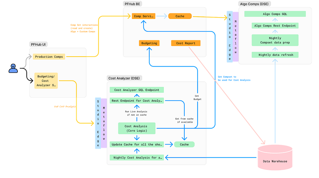
Flink supports reading and writing data to external systems, through connectors, which are components that allow your application to interact with stream-storage message brokers, databases, or object stores. Kinesis Data Streams is a popular source and destination for streaming applications. Flink provides both source and sink connectors for Kinesis Data Streams.

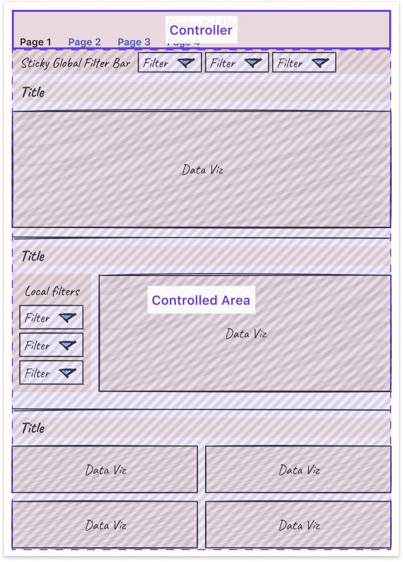
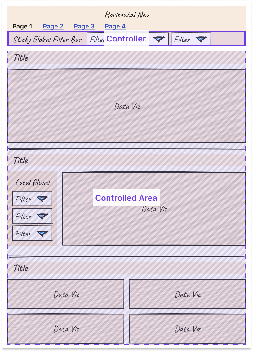
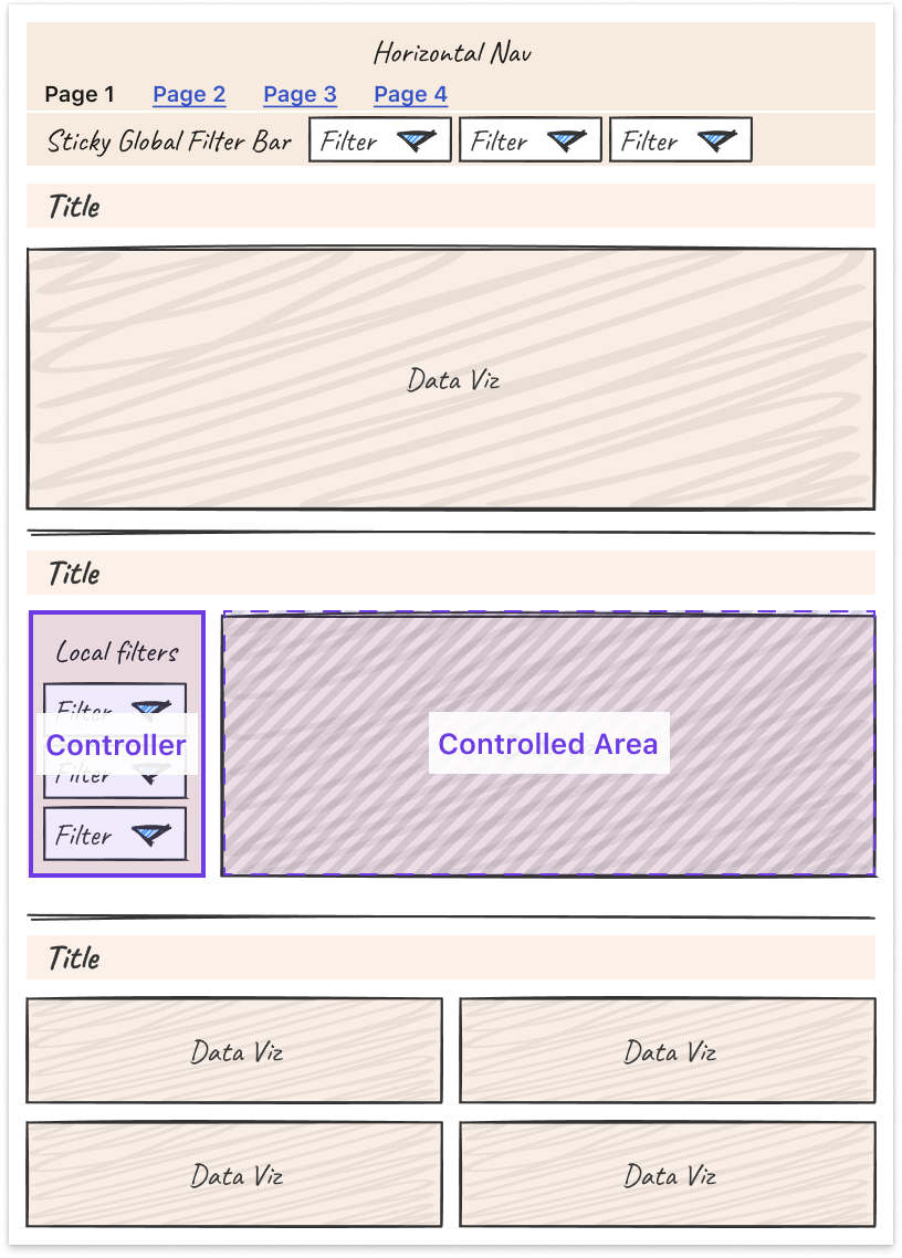
The following diagram illustrates a sample architecture.

Role of connectors in a Flink applications

Before proceeding further, it’s important to clarify three terms often used interchangeably in data streaming and in the Apache Flink documentation:

  • Kinesis Data Streams refers to the Amazon service
  • Kinesis source and Kinesis consumer refer to the Apache Flink components, in particular the source connectors, that allows reading data from Kinesis Data Streams
  • In this post, we use the term stream referring to a single Kinesis data stream

Introducing the new Flink Kinesis source connector

The launch of the version 5.0.0 of AWS connectors introduces a new connector for reading events from Kinesis Data Streams. The new connector is called Kinesis Streams Source and supersedes the Kinesis Consumer as the source connector for Kinesis Data Streams.

The new connector introduces several new features and adheres to the new Flink Source interface, and is compatible with Flink 2.x, the first major version release by the Flink community. Flink 2.x introduces a number of breaking changes, including removing the SourceFunction interface used by legacy connectors. The legacy Kinesis Consumer will no longer work with Flink 2.x.

Setting up the connector is slightly different than with the legacy Kinesis connector. Let’s start with the DataStream API.

How to use the new connector with the DataStream API

To add the new connector to your application, you need to update the connector dependency. For the DataStream API, the dependency has changed its name to flink-connector-aws-kinesis-streams.

At the time of writing, the latest connector version is 5.0.0 and it supports the most recent stable Flink versions, 1.19 and 1.20. The connector is also compatible with Flink 2.0, but no connector has been officially released for Flink 2.x yet. Assuming you are using Flink 1.20, the new dependency is the following:

<dependency>
    <groupId>org.apache.flink</groupId>
    <artifactId>flink-connector-aws-kinesis streams</artifactId>
    <version>5.0.0-1.20</version>
</dependency>

The connector uses the new Flink Source interface. This interface implements the new FLIP-27 standard, and replaces the legacy SourceFunction interface that has been deprecated. SourceFunction will be completely removed in Flink 2.x.

In your application, you can now use a fluent and expressive builder interface to instantiate and configure the source. The minimal setup only requires the stream Amazon Resource Name (ARN) and the deserialization schema:

KinesisStreamsSource<String> kdsSource = KinesisStreamsSource.<String>builder()
    .setStreamArn("arn:aws:kinesis:us-east-1:123456789012:stream/test-stream")
    .setDeserializationSchema(new SimpleStringSchema())
    .build();

The new source class is called KinesisStreamSource. Not to be confused with the legacy source, FlinkKinesisConsumer.

You can then add the source to the execution environment using the new fromSource() method. This method requires explicitly specifying the watermark strategy, along with a name for the source:

StreamExecutionEnvironment env = StreamExecutionEnvironment.getExecutionEnvironment();
// ...
DataStream<String> kinesisRecordsWithEventTimeWatermarks = env.fromSource(
    kdsSource,
    WatermarkStrategy.<String>forMonotonousTimestamps()
        .withIdleness(Duration.ofSeconds(1)),
    "Kinesis source");

These few lines of code introduce some of the main changes in the interface of the connector, which we discuss in the following sections.

Stream ARN

You can now define the Kinesis data stream ARN, as opposed to the stream name. This makes it simpler to consume from streams cross-Region and cross-account.

When running in Amazon Managed Service for Apache Flink, you only need to add to the application AWS Identity and Access Management (IAM) role permissions to access the stream. The ARN allows pointing to a stream located in a different AWS Region or account, without assuming roles or passing any external credentials.

Explicit watermark

One of the most important characteristics of the new Source interface is that you have to explicitly define a watermark strategy when you attach the source to the execution environment. If your application only implements processing-time semantics, you can specify WatermarkStrategy.noWatermarks().

This is an improvement in terms of code readability. Looking at the source, you know immediately which type of watermark you have, or if you don’t have any. Previously, many connectors were providing some type of default watermarks that the user could override. However, the default watermark of each connector was slightly different and confusing for the user.

With the new connector, you can achieve the same behavior as the legacy FlinkKinesisConsumer default watermarks, using WatermarkStrategy.forMonotonousTimestamps(), as shown in the previous example. This strategy generates watermarks based on the approximateArrivalTimestamp returned by Kinesis Data Streams. This timestamp corresponds to the time when the record was published to Kinesis Data Streams.

Idleness and watermark alignment

With the watermark strategy, you can additionally define an idleness, which allows the watermark to progress even when some shards of the stream are idle and receiving no records. Refer to Dealing With Idle Sources for more details about idleness and watermark generators.

A feature introduced by the new Source interface, and fully supported by the new Kinesis source, is watermark alignment. Watermark alignment works in the opposite direction of idleness. It slows down consuming from a shard that is progressing faster than others. This is particularly useful when replaying data from a stream, to reduce the volume of data buffered in the application state. Refer to Watermark alignment for more details.

Set up the connector with the Table API and SQL

Assuming you are using Flink 1.20, the dependency containing both Kinesis source and sink for the Table API and SQL is the following (both Flink 1.19 and 1.20 are supported, adjust the version accordingly):

<dependency>
    <groupId>org.apache.flink</groupId>
    <artifactId>flink-connector-kinesis</artifactId>
    <version>5.0.0-1.20</version>
</dependency>

This dependency contains both the new source and the legacy source. Refer to Versioning in case you are planning to use both in the same application.

When defining the source in SQL or the Table API, you use the connector name kinesis, as it was with the legacy source. However, many parameters have changed with the new source:

CREATE TABLE KinesisTable (
    `user_id` BIGINT,
    `item_id` BIGINT,
    `category_id` BIGINT,
    `behavior` STRING,
    `ts` TIMESTAMP(3)
)
PARTITIONED BY (user_id, item_id)
WITH (
    'connector' = 'kinesis',
    'stream.arn' = 'arn:aws:kinesis:us-east-1:012345678901:stream/my-stream-name',
    'aws.region' = 'us-east-1',
    'source.init.position' = 'LATEST',
    'format' = 'csv'
);

A couple of notable connector options changed from the legacy source are:

  • stream.arn specifies the stream ARN, as opposed to the stream name used in the legacy source.
  • init.initpos defines the starting position. This option works similarly to the legacy source, but the option name is different. It was previously scan.stream.initpos.

For the full list of connector options refer to Connector Options.

New features and improvements

In this section, we discuss the most important features introduced by the new connector. These features are available in the DataStream API, and also the Table API and SQL.

Ordering guarantees

The most important improvement introduced by the new connector is about ordering guarantees.

With Kinesis Data Streams, the order of the message is retained per partitionId. This is achieved by putting all records with the same partitionId in the same shard. However, when the stream scales, splitting or merging shards, records with the same partitionId end up in a new shard. Kinesis keeps track of the parent-child lineage when resharding happens.

Stream resharding

One known limitation of the legacy Kinesis source is that it was unable to follow the parent-child shard lineage. As a consequence, ordering could not be guaranteed when resharding happens. The problem was particularly relevant when the application replayed old messages from a stream that had been resharded because ordering would be lost. This also made watermark generation and event-time processing non-deterministic.

With the new connector, ordering is retained also when resharding happens. This is achieved following the parent-child shard lineage, and consuming all records from a parent shard before proceeding with the child shard.

How the connector follows shard lineage

A better default shard assigner

Each Kinesis data stream is comprised of many shards. Also, the Flink source operator runs in multiple parallel subtasks. The shard assigner is the component that decides how to assign the shards of the stream across the source subtasks. The shard assigner’s job is non-trivial, because shard split or merge operations (resharding) might happen when the stream scales up or down.

The new connector comes with a new default assigner, UniformShardAssigner. This assigner maintains uniform distribution of the stream partitionId across parallel subtasks, also when resharding happens. This is achieved by looking at the range of partition keys (HashKeyRange) of each shard.

This shard assigner was already available in the previous connector version, but for backward compatibility, it was not the default and you had to set it up explicitly. This is no longer the case with the new source. The old default shard assigner, the legacy FlinkKinesisConsumer, was evenly distributing shards (not partitionId) across subtasks. In this case, the actual data distribution might become uneven in the case of resharding, because of the combination of open and closed shards in the stream. Refer to Shard Assignment Strategy for more details.

Reduced JAR size

The size of the JAR file has been reduced by 99%, from about 60 MB down to 200 KB. This substantially reduces the size of the fat-JAR of your application using the connector. A smaller JAR can speed up many operations that require redeploying the application.

AWS SDK for Java 2.x

The new connector is based on the newer AWS SDK for Java 2.x, which adds several features and improves support for non-blocking I/O. This makes the connector future-proof because the AWS SDK v1 will reach end-of-support by end of 2025.

AWS SDK built-in retry strategy

The new connector relies on the AWS SDK built-in retry strategy, as opposed to a custom strategy implemented by the legacy connector. Relying on the AWS SDK improves the classification of some errors as retriable or non-retriable.

Removed dependency on the Kinesis Client Library and Kinesis Producer Library

The new connector package no longer includes the Kinesis Client Library (KCL) and Kinesis Producer Library (KPL), contributing to the substantial reduction of the JAR size that we have mentioned.

An implication of this change is that the new connector no longer supports de-aggregation out of the box. Unless you are publishing records to the stream using the KPL and you enabled aggregation, this will not make any difference for you. If your producers use KPL aggregation, you might consider implementing a custom DeserializationSchema to de-aggregate the records in the source.

Migrating from the legacy connector

Flink sources typically save the position in the checkpoint and savepoints, called snapshots in Amazon Managed Service for Apache Flink. When you stop and restart the application, or when you update the application to deploy a change, the default behavior is saving the source position in the snapshot just before stopping the application, and restoring the position when the application restarts. This allows Flink to provide exactly-once guarantees on the source.

However, due to the major changes introduced by the new KinesisSource, the saved state is no longer compatible with the legacy FlinkKinesisConsumer. This means that when you upgrade the source of an existing application, you can’t directly restore the source position from the snapshot.

For this reason, migrating your application to the new source requires some attention. The exact migration process depends on your use case. There are two general scenarios:

  • Your application uses the DataStream API and you are following Flink best practices defining a UID on each operator
  • Your application uses the Table API or SQL, or your application used the DataStream API and you are not defining a UID on each operator

Let’s cover each of these scenarios.

Your application uses the DataStream API and you are defining a UID on each operator

In this case, you might consider selectively resetting the state of the source operator, retaining any other application state. The general approach is as follows:

  1. Update your application dependencies and code, replacing the FlinkKinesisConsumer with the new KinesisSource.
  2. Change the UID of the source operator (use a different string). Leave all other operators’ UIDs This will selectively reset the state of the source while retaining the state of all other operators.
  3. Configure the source starting position using AT_TIMESTAMP and set the timestamp to just before the moment you will deploy the change. See Configuring Starting Position to learn how to set the starting position. We recommend passing the timestamp as a runtime property to make this more flexible. The configured source starting position is used only when the application can’t restore the state from a savepoint (or snapshot). In this case, we are deliberately forcing this, changing the UID of the source operator.
  4. Update the Amazon Managed Service for Apache Flink application, selecting the new JAR containing the modified application. Restart from the latest snapshot (default behavior) and select allowNonRestoredState = true. Without this flag, Flink would prevent restarting the application, not being able to restore the state of the old source that was saved in the snapshot. See Savepointing for more details about allowNonRestoredState.

This approach will cause the reprocessing of some records from the source, and internal state exactly-once consistency can be broken. Carefully evaluate the impact of reprocessing on your application, and the impact of duplicates on the downstream systems.

Your application uses the Table API or SQL, or your application used the DataStream API and you are not defining a UID on each operator

In this case, you can’t selectively reset the state of the source operator.

Why does this happen? When using the Table API or SQL, or the DataStream API without defining the operator’s UID explicitly, Flink automatically generates identifiers for all operators based on the structure of the job graph of your application. These identifiers are used to identify the state of each operator when saved in the snapshots, and to restore it to the correct operator when you restart the application.

Changes to the application might cause changes in the underlying data flow. This changes the auto-generated identifier. If you are using the DataStream API and you are specifying the UID, Flink uses your identifiers instead of the auto-generated identifies, and is able to map back the state to the operator, even when you make changes to the application. This is an intrinsic limitation of Flink, explained in Set UUIDs For All Operators. Enabling allowNonRestoredState does not solve this problem, because Flink is not able to map the state saved in the snapshot with the actual operators, after the changes.

In our migration scenario, the only option is resetting the state of your application. You can achieve this in Amazon Managed Service for Apache Flink by selecting Skip restore from snapshot (SKIP_RESTORE_FROM_SNAPSHOT) when you deploy the change that replaces the source connector.

After the application using the new source is up and running, you can switch back to the default behavior of when restarting the application, using the latest snapshots (RESTORE_FROM_LATEST_SNAPSHOT). This way, no data loss happens when the application is restarted.

Choosing the right connector package and version

The dependency version you need to pick is normally <connector-version>-<flink-version>. For example, the latest Kinesis connector version is 5.0.0. If you are using a Flink runtime version 1.20.x, your dependency for the DataStream API is 5.0.0-1.20.

For the most up-to-date connector versions, see Use Apache Flink connectors with Managed Service for Apache Flink.

Connector artifact

In previous versions of the connector (4.x and before), there were separate packages for the source and sink. This additional level of complexity has been removed with version 5.x.

For your Java application, or Python applications where you package JAR dependencies using Maven, as shown in the Amazon Managed Service for Apache Flink examples GitHub repository, the following dependency contains the new version of both source and sink connectors:

<dependency>
    <groupId>org.apache.flink</groupId>
    <artifactId>flink-connector-aws-kinesis-streams</artifactId>
    <version>5.0.0-1.20</version>
</dependency>

Make sure you’re using the latest available version. At the time of writing, this is 5.0.0. You can verify the available artifact versions in Maven Central. Also, use the correct version depending on your Flink runtime version. The previous example is for Flink 1.20.0.

Connector artifacts for Python application

If you use Python, we recommend packaging JAR dependencies using Maven, as shown in the Amazon Managed Service for Apache Flink examples GitHub repository. However, if you’re passing directly a single JAR to your Amazon Managed Service for Apache Flink application, you need to use the artifact that includes all transitive dependencies. In the case of the new Kinesis source and sink, this is called flink-sql-connector-aws-kinesis-streams. This artifact includes only the new source. Refer to Amazon Kinesis Data Streams SQL Connector for the right package, in case you want to use both the new and the legacy source.

Conclusion

The new Flink Kinesis source connector introduces many new features that improve stability and performance, and prepares your application for Flink 2.x. Support for watermark idleness and alignment is a particularly important feature if your application uses event-time semantics. The ability to retain record ordering improves data consistency, in particular when stream resharding happens, and when you replay old data from a stream that has been reshared.

You should carefully plan the change if you’re migrating your application from the legacy Kinesis source connector, and make sure you follow Flink’s best practices like specifying a UID on all DataStream operators.

You can find a working example of Java DataStream API application using the new connector, in the Amazon Managed Service for Apache Flink samples GitHub repository.

To learn more about the new Flink Kinesis source connector, refer to Amazon Kinesis Data Streams Connector and Amazon Kinesis Data Streams SQL Connector.


About the Author

Lorenzo NicoraLorenzo Nicora works as a Senior Streaming Solutions Architect at AWS, helping customers across EMEA. He has been building cloud-centered, data-intensive systems for over 25 years, working across industries both through consultancies and product companies. He has used open source technologies extensively and contributed to several projects, including Apache Flink.

Part 1: A Survey of Analytics Engineering Work at Netflix

Post Syndicated from Netflix Technology Blog original https://netflixtechblog.com/part-1-a-survey-of-analytics-engineering-work-at-netflix-d761cfd551ee

This article is the first in a multi-part series sharing a breadth of Analytics Engineering work at Netflix, recently presented as part of our annual internal Analytics Engineering conference. We kick off with a few topics focused on how we’re empowering Netflix to efficiently produce and effectively deliver high quality, actionable analytic insights across the company. Subsequent posts will detail examples of exciting analytic engineering domain applications and aspects of the technical craft.

At Netflix, we seek to entertain the world by ensuring our members find the shows and movies that will thrill them. Analytics at Netflix powers everything from understanding what content will excite and bring members back for more to how we should produce and distribute a content slate that maximizes member joy. Analytics Engineers deliver these insights by establishing deep business and product partnerships; translating business challenges into solutions that unblock critical decisions; and designing, building, and maintaining end-to-end analytical systems.

Each year, we bring the Analytics Engineering community together for an Analytics Summit — a 3-day internal conference to share analytical deliverables across Netflix, discuss analytic practice, and build relationships within the community. We covered a broad array of exciting topics and wanted to spotlight a few to give you a taste of what we’re working on across Analytics Engineering at Netflix!

DataJunction: Unifying Experimentation and Analytics

Yian Shang, Anh Le

At Netflix, like in many organizations, creating and using metrics is often more complex than it should be. Metric definitions are often scattered across various databases, documentation sites, and code repositories, making it difficult for analysts and data scientists to find reliable information quickly. This fragmentation leads to inconsistencies and wastes valuable time as teams end up reinventing metrics or seeking clarification on definitions that should be standardized and readily accessible.

Enter DataJunction (DJ). DJ acts as a central store where metric definitions can live and evolve. Once a metric owner has registered a metric into DJ, metric consumers throughout the organization can apply that same metric definition to a set of filtered records and aggregate to any dimensional grain.

As an example, imagine an analyst wanting to create a “Total Streaming Hours” metric. To add this metric to DJ, they need to provide two pieces of information:

  • The fact table that the metric comes from:

SELECT
account_id, country_iso_code, streaming_hours
FROM streaming_fact_table

  • The metric expression:

`SUM(streaming_hours)`

Then metric consumers throughout the organization can call DJ to request either the SQL or the resulting data. For example,

  • total_streaming_hours of each account:

dj.sql(metrics=[“total_streaming_hours”], dimensions=[“account_id”]))

  • total_streaming_hours of each country:

dj.sql(metrics=[“total_streaming_hours”], dimensions=[“country_iso_code”]))

  • total_streaming_hours of each account in the US:

dj.sql(metrics=[“total_streaming_hours”], dimensions=[“country_iso_code”], filters=[“country_iso_code = ‘US’”]))

The key here is that DJ can perform the dimensional join on users’ behalf. If country_iso_code doesn’t already exist in the fact table, the metric owner only needs to tell DJ that account_id is the foreign key to an `users_dimension_table` (we call this process “dimension linking”). DJ then can perform the joins to bring in any requested dimensions from `users_dimension_table`.

The Netflix Experimentation Platform heavily leverages this feature today by treating cell assignment as just another dimension that it asks DJ to bring in. For example, to compare the average streaming hours in cell A vs cell B, the Experimentation Platform relies on DJ to bring in “cell_assignment” as a user’s dimension (no different from country_iso_code). A metric can therefore be defined once in DJ and be made available across analytics dashboards and experimentation analysis.

DJ has a strong pedigree–there are several prior semantic layers in the industry (e.g. Minerva at Airbnb; dbt Transform, Looker, and AtScale as paid solutions). DJ stands out as an open source solution that is actively developed and stress-tested at Netflix. We’d love to see DJ easing your metric creation and consumption pain points!

LORE: How we’re democratizing analytics at Netflix

Apurva Kansara

At Netflix, we rely on data and analytics to inform critical business decisions. Over time, this has resulted in large numbers of dashboard products. While such analytics products are tremendously useful, we noticed a few trends:

  1. A large portion of such products have less than 5 MAU (monthly active users)
  2. We spend a tremendous amount of time building and maintaining business metrics and dimensions
  3. We see inconsistencies in how a particular metric is calculated, presented, and maintained across the Data & Insights organization.
  4. It is challenging to scale such bespoke solutions to ever-changing and increasingly complex business needs.

Analytics Enablement is a collection of initiatives across Data & Insights all focused on empowering Netflix analytic practitioners to efficiently produce and effectively deliver high-quality, actionable insights.

Specifically, these initiatives are focused on enabling analytics rather than on the activities that produce analytics (e.g., dashboarding, analysis, research, etc.).

As part of broad analytics enablement across all business domains, we invested in a chatbot to provide real insights to our end users using the power of LLM. One reason LLMs are well suited for such problems is that they tie the versatility of natural language with the power of data query to enable our business users to query data that would otherwise require sophisticated knowledge of underlying data models.

Besides providing the end user with an instant answer in a preferred data visualization, LORE instantly learns from the user’s feedback. This allows us to teach LLM a context-rich understanding of internal business metrics that were previously locked in custom code for each of the dashboard products.

Some of the challenges we run into:

  • Gaining user trust: To gain our end users’ trust, we focused on our model’s explainability. For example, LORE provides human-readable reasoning on how it arrived at the answer that users can cross-verify. LORE also provides a confidence score to our end users based on its grounding in the domain space.
  • Training: We created easy-to-provide feedback using 👍 and 👎 with a fully integrated fine-tuning loop to allow end-users to teach new domains and questions around it effectively. This allowed us to bootstrap LORE across several domains within Netflix.

Democratizing analytics can unlock the tremendous potential of data for everyone within the company. With Analytics enablement and LORE, we’ve enabled our business users to truly have a conversation with the data.

Leveraging Foundational Platform Data to enable Cloud Efficiency Analytics

J Han, Pallavi Phadnis

At Netflix, we use Amazon Web Services (AWS) for our cloud infrastructure needs, such as compute, storage, and networking to build and run the streaming platform that we love. Our ecosystem enables engineering teams to run applications and services at scale, utilizing a mix of open-source and proprietary solutions. In order to understand how efficiently we operate in this diverse technological landscape, the Data & Insights organization partners closely with our engineering teams to share key efficiency metrics, empowering internal stakeholders to make informed business decisions.

This is where our team, Platform DSE (Data Science Engineering), comes in to enable our engineering partners to understand what resources they’re using, how effectively they utilize those resources, and the cost associated with their resource usage. By creating curated datasets and democratizing access via a custom insights app and various integration points, downstream users can gain granular insights essential for making data-driven, cost-effective decisions for the business.

To address the numerous analytic needs in a scalable way, we’ve developed a two-component solution:

  1. Foundational Platform Data (FPD): This component provides a centralized data layer for all platform data, featuring a consistent data model and standardized data processing methodology. We work with different platform data providers to get inventory, ownership, and usage data for the respective platforms they own.
  2. Cloud Efficiency Analytics (CEA): Built on top of FPD, this component offers an analytics data layer that provides time series efficiency metrics across various business use cases. Once the foundational data is ready, CEA consumes inventory, ownership, and usage data and applies the appropriate business logic to produce cost and ownership attribution at various granularities.

As the source of truth for efficiency metrics, our team’s tenants are to provide accurate, reliable, and accessible data, comprehensive documentation to navigate the complexity of the efficiency space, and well-defined Service Level Agreements (SLAs) to set expectations with downstream consumers during delays, outages, or changes.

Looking ahead, we aim to continue onboarding platforms, striving for nearly complete cost insight coverage. We’re also exploring new use cases, such as tailored reports for platforms, predictive analytics for optimizing usage and detecting anomalies in cost, and a root cause analysis tool using LLMs.

Ultimately, our goal is to enable our engineering organization to make efficiency-conscious decisions when building and maintaining the myriad of services that allows us to enjoy Netflix as a streaming service. For more detail on our modeling approach and principles, check out this post!

Analytics Engineering is a key contributor to building our deep data culture at Netflix, and we are proud to have a large group of stunning colleagues that are not only applying but advancing our analytical capabilities at Netflix. The 2024 Analytics Summit continued to be a wonderful way to give visibility to one another on work across business verticals, celebrate our collective impact, and highlight what’s to come in analytics practice at Netflix.

To learn more, follow the Netflix Research Site, and if you are also interested in entertaining the world, have a look at our open roles!


Part 1: A Survey of Analytics Engineering Work at Netflix was originally published in Netflix TechBlog on Medium, where people are continuing the conversation by highlighting and responding to this story.

Recap of Amazon Redshift key product announcements in 2024

Post Syndicated from Neeraja Rentachintala original https://aws.amazon.com/blogs/big-data/recap-of-amazon-redshift-key-product-announcements-in-2024/

Amazon Redshift, launched in 2013, has undergone significant evolution since its inception, allowing customers to expand the horizons of data warehousing and SQL analytics. Today, Amazon Redshift is used by customers across all industries for a variety of use cases, including data warehouse migration and modernization, near real-time analytics, self-service analytics, data lake analytics, machine learning (ML), and data monetization.

Amazon Redshift made significant strides in 2024, rolling out over 100 features and enhancements. These improvements enhanced price-performance, enabled data lakehouse architectures by blurring the boundaries between data lakes and data warehouses, simplified ingestion and accelerated near real-time analytics, and incorporated generative AI capabilities to build natural language-based applications and boost user productivity.

2024 Redshift announcements summary

Figure1: Summary of the features and enhancements in 2024

Let’s walk through some of the recent key launches, including the new announcements at AWS re:Invent 2024.

Industry-leading price-performance

Amazon Redshift offers up to three times better price-performance than alternative cloud data warehouses. Amazon Redshift scales linearly with the number of users and volume of data, making it an ideal solution for both growing businesses and enterprises. For example, dashboarding applications are a very common use case in Redshift customer environments where there is high concurrency and queries require quick, low-latency responses. In these scenarios, Amazon Redshift offers up to seven times better throughput per dollar than alternative cloud data warehouses, demonstrating its exceptional value and predictable costs.

Performance improvements

Over the past few months, we have introduced a number of performance improvements to Redshift. First query response times for dashboard queries have significantly improved by optimizing code execution and reducing compilation overhead. We have enhanced data sharing performance with improved metadata handling, resulting in data sharing first query execution that is up to four times faster when the data sharing producer’s data is being updated. We have enhanced autonomics algorithms to generate and implement smarter and quicker optimal data layout recommendations for distribution and sort keys, further optimizing performance. We have launched new RA3.large instances, a new smaller size RA3 node type, to offer better flexibility in price-performance and provide a cost-effective migration option for customers using DC2.large instances. Additionally, we have rolled out AWS Graviton in Serverless, offering up to 30% better price-performance, and expanded concurrency scaling to support more types of write queries, enabling an even greater ability to maintain consistent performance at scale. These improvements collectively reinforce Amazon Redshift’s focus as a leading cloud data warehouse solution, offering unparalleled performance and value to customers.

General availability of multi-data warehouse writes

Amazon Redshift allows you to seamlessly scale with multi-cluster deployments. With the introduction of RA3 nodes with managed storage in 2019, customers obtained flexibility to scale and pay for compute and storage independently. Redshift data sharing, launched in 2020, enabled seamless cross-account and cross-Region data collaboration and live access without physically moving the data, while maintaining transactional consistency. This allowed customers to scale read analytics workloads and offered isolation to help maintain SLAs for business-critical applications. At re:Invent 2024, we announced the general availability of multi-data warehouse writes through data sharing for Amazon Redshift RA3 nodes and Serverless. You can now start writing to shared Redshift databases from multiple Redshift data warehouses in just a few clicks. The written data is available to all the data warehouses as soon as it’s committed. This allows your teams to flexibly scale write workloads such as extract, transform, and load (ETL) and data processing by adding compute resources of different types and sizes based on individual workloads’ price-performance requirements, as well as securely collaborate with other teams on live data for use cases such as customer 360.

General availability of AI-driven scaling and optimizations

The launch of Amazon Redshift Serverless in 2021 marked a significant shift, eliminating the need for cluster management while paying for what you use. Redshift Serverless and data sharing enabled customers to easily implement distributed multi-cluster architectures for scaling analytics workloads. In 2024, we launched Serverless in 10 more regions, improved functionality, and added support for a capacity configuration of 1024 RPUs, allowing you to bring larger workloads onto Redshift. Redshift Serverless is also now even more intelligent and dynamic with the new AI-driven scaling and optimization capabilities. As a customer, you choose whether you want to optimize your workloads for cost, performance, or keep it balanced, and that’s it. Redshift Serverless works behind the scenes to scale the compute up and down and deploys optimizations to meet and maintain the performance levels, even when workload demands change. In internal tests, AI-driven scaling and optimizations showcased up to 10 times price-performance improvements for variable workloads.

Seamless Lakehouse architectures

Lakehouse brings together flexibility and openness of data lakes with the performance and transactional capabilities of data warehouses. Lakehouse allows you to use preferred analytics engines and AI models of your choice with consistent governance across all your data. At re:Invent 2024, we unveiled the next generation of Amazon SageMaker, a unified platform for data, analytics, and AI. This launch brings together widely adopted AWS ML and analytics capabilities, providing an integrated experience for analytics and AI with a re-imagined lakehouse and built-in governance.

General availability of Amazon SageMaker Lakehouse

Amazon SageMaker Lakehouse unifies your data across Amazon S3 data lakes and Redshift data warehouses, enabling you to build powerful analytics and AI/ML applications on a single copy of data. SageMaker Lakehouse provides the flexibility to access and query your data using Apache Iceberg open standards so that you can use your preferred AWS, open source, or third-party Iceberg-compatible engines and tools. SageMaker Lakehouse offers integrated access controls and fine-grained permissions that are consistently applied across all analytics engines and AI models and tools. Existing Redshift data warehouses can be made available through SageMaker Lakehouse in just a simple publish step, opening up all your data warehouse data with Iceberg REST API. You can also create new data lake tables using Redshift Managed Storage (RMS) as a native storage option. Check out the Amazon SageMaker Lakehouse: Accelerate analytics & AI presented at re:Invent 2024.

Preview of Amazon SageMaker Unified Studio

Amazon SageMaker Unified Studio is an integrated data and AI development environment that enables collaboration and helps teams build data products faster. SageMaker Unified Studio brings together functionality and tools from a mix of standalone studios, query editors, and visual tools available today in Amazon EMR, AWS Glue, Amazon Redshift, Amazon Bedrock, and the existing Amazon SageMaker Studio, into one unified experience. With SageMaker Unified Studio, various users such as developers, analysts, data scientists, and business stakeholders can seamlessly work together, share resources, perform analytics, and build and iterate on models, fostering a streamlined and efficient analytics and AI journey.

Amazon Redshift SQL analytics on Amazon S3 Tables

At re:Invent 2024, Amazon S3 introduced Amazon S3 Tables, a new bucket type that is purpose-built to store tabular data at scale with built-in Iceberg support. With table buckets, you can quickly create tables and set up table-level permissions to manage access to your data lake. Amazon Redshift introduced support for querying Iceberg data in data lakes last year, and now this capability is extended to seamlessly querying S3 Tables. S3 Tables customers create are also available as part of the Lakehouse for consumption by other AWS and third-party engines.

Data lake query performance

Amazon Redshift offers high-performance SQL capabilities on SageMaker Lakehouse, whether the data is in other Redshift warehouses or in open formats. We enhanced support for querying Apache Iceberg data and improved the performance of querying Iceberg up to threefold year-over-year. A number of optimizations contribute to these speed-ups in performance, including integration with AWS Glue Data Catalog statistics, improved data and metadata filtering, dynamic partition elimination, faster/parallel processing of Iceberg manifest files, and scanner improvements. In addition, Amazon Redshift now supports incremental refresh support for materialized views on data lake tables to eliminate the need for recomputing the materialized view when new data arrives, simplifying how you build interactive applications on S3 data lakes.

Simplified ingestion and near real-time analytics

In this section, we share the improvements regarding simplified ingestion and near real-time analytics that enable you to get faster insights over fresher data.

Zero-ETL integration with AWS databases and third-party enterprise applications

Amazon Redshift first launched zero-ETL integration between Amazon Aurora MySQL-Compatible Edition, enabling near real-time analytics on petabytes of transactional data from Aurora. This capability has since expanded to support Amazon Aurora PostgreSQL-Compatible Edition, Amazon Relational Database Service (Amazon RDS) for MySQL, and Amazon DynamoDB, and includes additional features such as data filtering to selectively extract tables and schemas using regular expressions, support for incremental and auto-refresh materialized views on replicated data, and configurable change data capture (CDC) refresh rates.

Building on this innovation, at re:Invent 2024, we launched support for zero-ETL integration with eight enterprise applications, specifically Salesforce, Zendesk, ServiceNow, SAP, Facebook Ads, Instagram Ads, Pardot, and Zoho CRM. With this new capability, you can efficiently extract and load valuable data from your customer support, relationship management, and Enterprise Resource Planning (ERP) applications directly into your Redshift data warehouse for analysis. This seamless integration eliminates the need for complex, custom ingestion pipelines for ingesting the data, accelerating time to insights.

General availability of auto-copy

Auto-copy simplifies data ingestion from Amazon S3 into Amazon Redshift. This new feature enables you to set up continuous file ingestion from your Amazon S3 prefix and automatically load new files to tables in your Redshift data warehouse without the need for additional tools or custom solutions.

Streaming ingestion from Confluent Managed Cloud and self-managed Apache Kafka clusters

Amazon Redshift now supports streaming ingestion from Confluent Managed Cloud and self-managed Apache Kafka clusters on Amazon EC2instances, expanding its capabilities beyond Amazon Kinesis Data Streams and Amazon Managed Streaming for Apache Kafka (Amazon MSK). With this update, you can ingest data from a wider range of streaming sources directly into your Redshift data warehouses for near real-time analytics use cases such as fraud detection, logistics monitoring and clickstream analysis.

Generative AI capabilities

In this section, we share the improvements generative AI capabilities.

Amazon Q generative SQL for Amazon Redshift

We announced the general availability of Amazon Q generative SQL for Amazon Redshift feature in the Redshift Query Editor. Amazon Q generative SQL boosts productivity by allowing users to express queries in natural language and receive SQL code recommendations based on their intent, query patterns, and schema metadata. The conversational interface enables users to get insights faster without extensive knowledge of the database schema. It leverages generative AI to analyze user input, query history, and custom context like table/column descriptions and sample queries to provide more relevant and accurate SQL recommendations. This feature accelerates the query authoring process and reduces the time required to derive actionable data insights.

Amazon Redshift integration with Amazon Bedrock

We announced integration of Amazon Redshift with Amazon Bedrock, enabling you to invoke large language models (LLMs) from simple SQL commands on your data in Amazon Redshift. With this new feature, you can now effortlessly perform generative AI tasks such as language translation, text generation, summarization, customer classification, and sentiment analysis on your Redshift data using popular foundation models (FMs) like Anthropic’s Claude, Amazon Titan, Meta’s Llama 2, and Mistral AI. You can invoke these models using familiar SQL commands, making it simpler than ever to integrate generative AI capabilities into your data analytics workflows.

Amazon Redshift as a knowledge base in Amazon Bedrock

Amazon Bedrock Knowledge Bases now supports natural language querying to retrieve structured data from your Redshift data warehouses. Using advanced natural language processing, Amazon Bedrock Knowledge Bases can transform natural language queries into SQL queries, allowing users to retrieve data directly from the source without the need to move or preprocess the data. A retail analyst can now simply ask “What were my top 5 selling products last month?”, and Amazon Bedrock Knowledge Bases automatically translates that query into SQL, runs the query against Redshift, and returns the results—or even provides a summarized narrative response. To generate accurate SQL queries, Amazon Bedrock Knowledge Bases uses database schema, previous query history, and other contextual information that is provided about the data sources.

Launch summary

Following is the launch summary which provides the announcement links and reference blogs for the key announcements.

Industry-leading price-performance:

Reference Blogs:

Seamless Lakehouse architectures:

Reference Blogs:

Simplified ingestion and near real-time analytics:

Reference Blogs:

Generative AI:

Reference Blogs:

Conclusion

We continue to innovate and evolve Amazon Redshift to meet your evolving data analytics needs. We encourage you to try out the latest features and capabilities. Watch the Innovations in AWS analytics: Data warehousing and SQL analytics session from re:Invent 2024 for further details. If you need any support, reach out to us. We are happy to provide architectural and design guidance, as well as support for proof of concepts and implementation. It’s Day 1!


About the Author

Neeraja Rentachintala is Director, Product Management with AWS Analytics, leading Amazon Redshift and Amazon SageMaker Lakehouse. Neeraja is a seasoned technology leader, bringing over 25 years of experience in product vision, strategy, and leadership roles in data products and platforms. She has delivered products in analytics, databases, data integration, application integration, AI/ML, and large-scale distributed systems across on-premises and the cloud, serving Fortune 500 companies as part of ventures including MapR (acquired by HPE), Microsoft SQL Server, Oracle, Informatica, and Expedia.com

How DeNA Co., Ltd. accelerated anonymized data quality tests up to 100 times faster using Amazon Redshift Serverless and dbt

Post Syndicated from Momota Sasaki original https://aws.amazon.com/blogs/big-data/how-dena-co-ltd-accelerated-anonymized-data-quality-tests-up-to-100-times-faster-using-amazon-redshift-serverless-and-dbt/

This blog was co-authored by DeNA Co., Ltd. and Amazon Web Services Japan.

DeNA Co., Ltd. (DeNA) engages in a variety of businesses, from games and live communities to sports & the community and healthcare & medical, under our mission to delight people beyond their wildest dreams. Among these, the healthcare & medical business handles particularly sensitive data. To comply with their data policies for sensitive data, this healthcare & medical business set the following requirements for their data processing:

  • Process data in compliance with data policies – Mask or delete sensitive data as necessary to transform into anonymized data. Prevent the inclusion of invalid values in categorical data and process data without any data loss.
  • Conduct data quality tests on anonymized data in compliance with data policies – Conduct data quality tests to quickly identify and address data quality issues, maintaining high-quality data at all times.

This post introduces a case study where DeNA combined Amazon Redshift Serverless and dbt (dbt Core) to accelerate data quality tests in their business.

The challenge

Data quality tests require performing 1,300 tests on 10 TB of data monthly. Previously, DeNA ran Python-based batch jobs on Amazon Elastic Compute Cloud (Amazon EC2) to perform these data quality tests. As business and data volume grew over time, DeNA started to face the following challenges:

  • Performance – Data quality tests took days to weeks to complete because engineers hadn’t designed the batch jobs to handle big data.
  • Cost – Costs increased due to the batch job design, particularly for large datasets. The implementation required loading data into memory for processing. When handling large table data, DeNA needed to use large memory-optimized EC2 instances.
  • Maintainability – The batch job implementations varied significantly between engineers, leading to high maintenance overhead, because the required knowledge was siloed among individual engineers.

The switch to Redshift Serverless and dbt

To address these challenges, DeNA decided to adopt Redshift Serverless and dbt (an open source data transformation tool) for the following key reasons:

  • Scalable and cost-effective processing with Redshift Serverless
  • Standardized and maintainable data quality tests with dbt

This decision was made after careful comparison of alternative solutions. DeNA initially considered parallelizing the existing Python-based batch jobs but rejected this approach due to the high maintenance overhead and siloed knowledge associated with the batch jobs. Instead, DeNA decided to use dbt, which DeNA has been using in their healthcare & medical business, and connect it to an AWS service capable of large-scale distributed processing. dbt provides a SQL-first templating engine for repeatable and extensible data transformations, including a data tests feature, which allows verifying data models and tables against expected rules and conditions using SQL. By using dbt, DeNA could standardize the technical stack, implement data quality tests in maintainable SQL, and connect dbt to a managed service for scalable and cost-effective processing.

AWS offers several services that are compatible with dbt, including Amazon Redshift and AWS Glue. DeNA selected Redshift Serverless, primarily due to its serverless nature, optimal cost-performance, and the superior processing performance for structured data typical of a data warehouse service.

Solution overview

DeNA designed the following architecture using AWS serverless services.

The workflow consists of the following high-level steps and key design points:

  1. The source system stores the target data for the data quality tests in Amazon Simple Storage Service (Amazon S3). When new data files are added, Amazon EventBridge invokes an AWS Step Functions state machine (workflow). To make sure all files for target data are delivered, the source system stores a completion file in Amazon S3.
  2. dbt runs on Amazon Elastic Container Service (Amazon ECS) using AWS Fargate, an AWS serverless container service. DeNA selected Amazon ECS because it allows running dbt in a serverless, pay-per-use manner, and DeNA had prior experience developing and operating applications using Amazon ECS. To allow the containers to securely access Redshift Serverless, DeNA used the pass sensitive data to an ECS container feature to pass sensitive credentials that are stored in AWS Secrets Manager to the containers using an ECS task execution IAM role.
  3. DeNA segmented Redshift Serverless into separate workgroups for access control. Operation personnel may need to access the Redshift Serverless database using the Query Editor V2 to investigate issues with data quality tests, while maintaining strict access control. Redshift Serverless allows fine-grained access control to data by using database security features, similar to how the GRANT command is used in database products. However, in this workload, DeNA chose to use AWS Identity and Access Management (IAM) to control access to the workgroups at IAM level. This allowed DeNA to restrict access to specific Redshift Serverless workgroups based on users’ IAM roles, enabling unified management of authorization through IAM. Additionally, by separating the workgroups, DeNA could individually adjust Redshift Processing Units (RPUs) per workgroup, contributing to cost optimization.
  4. Amazon ECS sends execution logs of dbt running to Amazon CloudWatch Logs for observability. DeNA used metric filters to convert the logs into CloudWatch metrics, then created alarms based on these metrics. When triggered, these alarms invoke AWS Lambda functions using Amazon Simple Notification Service (Amazon SNS). The Lambda functions create result reports of dbt running and data quality tests and send them to an internal chat application. DeNA visualizes the results of data quality tests using the elementary CLI, a dbt-based data observability solution. This workflow enables even non-engineers to track data quality status effectively.

Outcomes

DeNA successfully addressed all the challenges they faced by designing the solution and migrating to a new platform:

  • Performance – Improved performance up to 100 times faster by reducing processing time from days or weeks to 1–2 hours. A certain data quality test that previously took 877 minutes now completes in 1 minute, thanks to the large-scale distributed processing capabilities of Redshift Serverless.
  • Cost – Reduced costs by 90% with AWS serverless services. Optimized expenses by incurring costs only for data quality tests.
  • Maintainability – Standardized the technical stack with dbt, eliminating siloed knowledge from custom programs. dbt’s data tests feature simplified the implementation of data quality tests. The elementary CLI improved the observability of data quality tests for non-engineers. AWS serverless services virtually eliminated the operational overhead for managing the workload infrastructure.

Conclusion

This post demonstrated how DeNA was able to securely and efficiently accelerate their data quality tests by combining Redshift Serverless and dbt. This combination is not only effective for DeNA’s use case but also applicable to various business use cases across different industries.

For more information on the combination of Redshift Serverless and dbt, refer to the following resources:


About the Author

Momota Sasaki is an Engineering Manager at DeSC Healthcare, a subsidiary of DeNA. He joined DeNA in 2021 and was seconded to DeSC Healthcare. Since then, he has been consistently involved in the healthcare business, leading and promoting the development and operation of the data platform.

Kaito Tawara is a Data Engineer at DeSC Healthcare, a subsidiary of DeNA, focusing on improving healthcare data platforms. After gaining experience in backend development for web systems and data science, he transitioned to data engineering. He joined DeNA in 2023 and was seconded to DeSC Healthcare. Currently, he works remotely from Nagoya-city, contributing to the enhancement of healthcare data platforms.

Shota Sato is an Analytics Specialist Solution Architect at AWS Japan, focusing on data analytics solutions powered by AWS for digital native business customers.

Top 6 game changers from AWS that redefine streaming data

Post Syndicated from Sai Maddali original https://aws.amazon.com/blogs/big-data/top-6-game-changers-from-aws-that-redefine-streaming-data/

Recently, AWS introduced over 50 new capabilities across its streaming services, significantly enhancing performance, scale, and cost-efficiency. Some of these innovations have tripled performance, provided 20 times faster scaling, and reduced failure recovery times by up to 90%. We have made it nearly effortless for customers to bring real-time context to AI applications and lakehouses.

In this post, we discuss the top six game changers that will redefine AWS streaming data.

Amazon MSK Express brokers: Kafka reimagined for AWS

AWS offers Express brokers for Amazon Managed Streaming for Apache Kafka (Amazon MSK)—a transformative breakthrough for customers needing high-throughput Kafka clusters that scale faster and cost less. With Express brokers, we are reimagining Kafka’s compute and storage decoupling to unlock performance and elasticity benefits. Express brokers offer up to three times more throughput than a comparable standard Apache Kafka broker, virtually unlimited storage, instant storage scaling, compute scaling in minutes vs. hours, and 90% faster recovery from failures compared to standard Kafka brokers. Customers can provision capacity in minutes without complex calculations, benefit from preset Kafka configurations, and scale capacity in a few clicks. Express brokers provide the same low-latency performance as standard Kafka, are 100% native Kafka, and offer key Amazon MSK features. There are no storage limits per broker and you only pay for the storage you use. With Express brokers for Amazon MSK, enterprises can expand their Kafka usage to support even more mission-critical use cases, while keeping both operational overhead and overall infrastructure costs low.

Amazon Kinesis Data Streams On-Demand: Scaling new heights

Amazon Kinesis Data Streams On-Demand makes it uncomplicated for developers to stream gigabytes per second of data without managing capacity or servers. Developers can create a new on-demand data stream or convert an existing data stream to on-demand mode with a single click. Kinesis Data Streams On-Demand now automatically scales to 10 GBps of write throughput and 200 GBps of read throughput per stream, a fivefold increase. Customers will automatically get this fivefold increase in scale without the need to take any action.

Streaming data to Iceberg tables in lakehouses

Enterprises are embracing lakehouses and open table formats such as Apache Iceberg to unlock value from their data. Amazon Data Firehose now supports seamless integration with Iceberg tables on Amazon Simple Storage Service (Amazon S3). Customers can stream data into Iceberg tables in Amazon S3 without any management overhead. Data Firehose compacts small files, minimizing storage inefficiencies and enhancing read performance. Data Firehose also handles schema changes while in flight, to provide consistency across evolving datasets. Because Data Firehose is fully managed and serverless, it scales seamlessly to handle high throughput streaming workloads, providing reliable and fast delivery of data. This capability also makes it straightforward to stream data stored in MSK topics and Kinesis data streams into Iceberg tables, potentially eliminating the need for custom extract, transform, and load (ETL) pipelines. Customers can now bring the power of real-time data to Iceberg tables without any additional effort—a paradigm shift for businesses. Additionally, Kinesis Data Firehose serves as a versatile bridge to stream real-time data from MSK clusters and Kinesis Data Streams into the newly launched Amazon S3 Tables and Amazon SageMaker Lakehouse. This unified approach facilitates more effective data management and analysis, supporting data-driven decision-making across the enterprise.

Unlocking the value of data stored in databases with change replication to Iceberg tables

Delivering database changes into Iceberg tables is emerging as a common pattern. Now in public preview, Data Firehose supports capturing changes made in databases such as PostgreSQL and MySQL and replicating the updates to Iceberg tables on Amazon S3. The integration uses change data capture (CDC) to continuously deliver database updates, eliminating manual processes and reducing operational overhead. Data Firehose automates tasks such as schema alignment and partitioning, making sure tables are optimized for analytics. With this new capability, customers can streamline their end-to-end data pipeline, allowing them to continually feed fresh data into an Iceberg table without needing to build a custom data pipeline.

Real-time context to generative AI applications

Customers tell us how they want to gain insights from generative AI by being able to bring their data to large language models (LLMs). They want to bring data as it’s generated to pre-trained models for more accurate and up-to-date responses. Amazon MSK provides a blueprint that allows customers to combine the context from real-time data with the powerful LLMs on Amazon Bedrock to generate accurate, up-to-date AI responses without writing custom code. Developers can configure the blueprint to generate vector embeddings using Amazon Bedrock embedding models, then index those embeddings in Amazon OpenSearch Service for data captured and stored in MSK topics. Customers can also improve the efficiency of data retrieval using built-in support for data chunking techniques from LangChain, an open source library, supporting high-quality inputs for model ingestion.

More cost-effective and reliable stream processing

AWS offers the Kinesis Client Library (KCL), an open source library, that simplifies the development of stream processing applications with Kinesis Data Streams. With KCL 3.0, customers can reduce compute costs to process streaming data by up to 33% compared to previous KCL versions. KCL 3.0 introduces an enhanced load balancing algorithm that continuously monitors the resource utilization of the stream processing workers and automatically redistributes the load from over-utilized workers to underutilized workers. These changes also enhance scalability and the overall efficiency of processing large volumes of streaming data. We have also made improvements to our Amazon Managed Service for Apache Flink. We offer the latest Flink versions on Amazon Managed Service for Apache Flink for customers to benefit from the latest innovations. Customers can also upgrade their existing applications to use new Flink versions with a new in-place version upgrade feature. Amazon Managed Service for Apache Flink now offers per-second billing, so customers can run their Flink applications for a short period and only pay for what they use, down to the nearest second.

Conclusion

AWS has made new innovations in data streaming services, bringing compelling value to customers on performance, scalability, elasticity, and ease of use. These advancements empower businesses to use real-time data more effectively, which modernizes the way for the next generation of data-driven applications and analytics. It is still Day 1!


About the authors

Sai Maddali is a Senior Manager Product Management at AWS who leads the product team for Amazon MSK. He is passionate about understanding customer needs, and using technology to deliver services that empowers customers to build innovative applications. Besides work, he enjoys traveling, cooking, and running.

Bill Crew is a Senior Product Marketing Manager. He is the lead marketer for Streaming and Messaging Services at AWS. Including Amazon Managed Streaming for Apache Kafka (Amazon MSK), Amazon Managed Service for Apache Flink, Amazon Data Firehose, Amazon Kinesis Data Streams, Amazon Message Broker (Amazon MQ), Amazon Simple Queue Service (Amazon SQS), and Amazon Simple Notification Services (Amazon SNS). Besides work, he enjoys collecting vintage vinyl records.

Introducing a new unified data connection experience with Amazon SageMaker Lakehouse unified data connectivity

Post Syndicated from Chiho Sugimoto original https://aws.amazon.com/blogs/big-data/introducing-a-new-unified-data-connection-experience-with-amazon-sagemaker-lakehouse-data-connectivity/

The need to integrate diverse data sources has grown exponentially, but there are several common challenges when integrating and analyzing data from multiple sources, services, and applications. First, you need to create and maintain independent connections to the same data source for different services. Second, the data connectivity experience is inconsistent across different services. For each service, you need to learn the supported authorization and authentication methods, data access APIs, and framework to onboard and test data sources. Third, some services require you to set up and manage compute resources used for federated connectivity, and capabilities like connection testing and data preview aren’t available in all services. This fragmented, repetitive, and error-prone experience for data connectivity is a significant obstacle to data integration, analysis, and machine learning (ML) initiatives.

To solve for these challenges, we launched Amazon SageMaker Lakehouse unified data connectivity. This feature offers the following capabilities and benefits:

  • With SageMaker Lakehouse unified data connectivity, you can set up a connection to a data source using a connection configuration template that is standardized for multiple services. Amazon SageMaker Unified Studio, AWS Glue, and Amazon Athena can share and reuse the same connection with proper permission configuration.
  • SageMaker Lakehouse unified data connectivity supports standard methods for data source connection authorization and authentications, such as basic authorization and OAuth2. This approach simplifies your data journey and helps you meet your security requirements.
  • The SageMaker Lakehouse data connection testing capability boosts your confidence in established connections. With the ability to browse metadata, you can understand the structure and schema of the data source, identify relevant tables and fields, and discover useful data assets you may not be aware of.
  • SageMaker Lakehouse unified data connectivity’s data preview capability helps you map source fields to target schemas, identify needed data transformation, and plan data standardization and normalization steps.
  • SageMaker Lakehouse unified data connectivity provides a set of APIs for you to use without the need to learn different APIs for various data sources, promoting coding efficiency and productivity.

With SageMaker Lakehouse unified data connectivity, you can confidently connect, explore, and unlock the full value of your data across AWS services and achieve your business objectives with agility.

This post demonstrates how SageMaker Lakehouse unified data connectivity helps your data integration workload by streamlining the establishment and management of connections for various data sources.

Solution overview

In this scenario, an e-commerce company sells products on their online platform. The product data is stored on Amazon Aurora PostgreSQL-Compatible Edition. Their existing business intelligence (BI) tool runs queries on Athena. Furthermore, they have a data pipeline to perform extract, transform, and load (ETL) jobs when moving data from the Aurora PostgreSQL database cluster to other data stores.

Now they have a new requirement to allow ad-hoc queries through SageMaker Unified Studio to enable data engineers, data analysts, sales representatives, and others to take advantage of its unified experience.

In the following sections, we demonstrate how to set up this connection and run queries using different AWS services.

Prerequisites

Before you begin, make sure you have the followings:

  • An AWS account.
  • A SageMaker Unified Studio domain.
  • An Aurora PostgreSQL database cluster.
  • A virtual private cloud (VPC) and private subnets required for SageMaker Unified Studio.
  • An Amazon Simple Storage Service (Amazon S3) bucket to store output from the AWS Glue ETL jobs. In the following steps, replace amzn-s3-demo-destination-bucket with the name of the S3 bucket.
  • An AWS Glue Data Catalog database. In the following steps, replace <your_database> with the name of your database.

Create an IAM role for the AWS Glue job

You can either create a new AWS Identity and Access Management (IAM) role or use an existing role that has permission to access the AWS Glue output bucket and AWS Secrets Manager.

If you want to create a new one, complete the following steps:

  1. On the IAM console, in the navigation pane, choose Roles.
  2. Choose Create role.
  3. For Trusted entity type, choose AWS service.
  4. For Service or use case, choose Glue.
  5. Choose Next.
  6. For Add permissions, choose AWSGlueServiceRole, then choose Next.
  7. For Role name, enter a role name (for this post, GlueJobRole-demo).
  8. Choose Create role.
  9. Choose the created IAM role.
  10. Under Permissions policies, choose Add permission and Create inline policy.
  11. For Policy editor, choose JSON, and enter the following policy:
    {
         "Version": "2012-10-17",
         "Statement": [
             {
                 "Effect": "Allow",
                 "Action": [
                     "s3:List*",
                     "s3:GetObject",
                     "s3:PutObject",
                     "s3:DeleteObject"
                 ],
                 "Resource": [
                     "arn:aws:s3:::amzn-s3-demo-destination-bucket/*",
                     "arn:aws:s3:::amzn-s3-demo-destination-bucket"
                 ]
             },
            {
                "Effect": "Allow",
                "Action": [
                    "secretsmanager:GetSecretValue"
                ],
                "Resource": [
                    "arn:aws:secretsmanager:<region>:<account-id>:secret:SageMakerUnifiedStudio-Glue-postgresql_source-*"
                ]
            }
         ]
     }

  12. Choose Next.
  13. For Policy name, enter a name for your policy.
  14. Choose Create policy.

Create a SageMaker Lakehouse data connection

Let’s get started with the unified data connection experience. The first step is to create a SageMaker Lakehouse data connection. Complete the following steps:

  1. Sign in to your SageMaker Unified Studio.
  2. Open your project.
  3. On your project, in the navigation pane, choose Data.
  4. Choose the plus sign.
  5. For Add data source, choose Add connection. Choose Next.
  6. Select PostgreSQL, and choose Next.
  7. For Name, enter postgresql_source.
  8. For Host, enter your host name of your Aurora PostgreSQL database cluster.
  9. For Port, enter your port number of your Aurora PostgreSQL database cluster (by default, it’s 5432).
  10. For Database, enter your database name.
  11. For Authentication, select Username and password.
  12. Enter your username and password.
  13. Choose Add data.

After the completion, it will create a new AWS Secrets Manager secret with a name like SageMakerUnifiedStudio-Glue-postgresql_source to securely store the specified username and password. It also creates a Glue connection with the same name postgresql_source.

Now you have a unified connection for Aurora PostgreSQL-Compatible.

Load data into the PostgreSQL database through the notebook

You will use a JupyterLab notebook on SageMaker Unified Studio to load sample data from an S3 bucket into a PostgreSQL database using Apache Spark.

  1. On the top left menu, choose Build, and under IDE & APPLICATIONS, choose JupyterLab.
  2. Choose Python 3 under Notebook.
  3. For the first cell, choose Local Python, python, enter following code, and run the cell:
    %%configure -f -n project.spark
    {
        "glue_version": "4.0"
    }

  4. For the second cell, choose PySpark, spark, enter following code, and run the cell:
    # Read sample data from S3 bucket
    df = spark.read.parquet("s3://aws-bigdata-blog/generated_synthetic_reviews/data/product_category=Apparel/")
    
    # Preview the data
    df.show()

The code snippet reads the sample data Parquet files from the specified S3 bucket location and stores the data in a Spark DataFrame named df. The df.show() command displays the first 20 rows of the DataFrame, allowing you to preview the sample data in a tabular format. Next, you will load this sample data into a PostgreSQL database.

  1. For the third cell, choose PySpark, spark, enter following code, and run the cell (replace <account-id> with your AWS account ID):
    import boto3
    import ast
    
    # replace you account ID before running this cell
    
    # Get secret
    secretsmanager_client = boto3.client('secretsmanager')
    get_secret_value_response = secretsmanager_client.get_secret_value(
        SecretId='SageMakerUnifiedStudio-Glue-postgresql_source' # replace the secret name if needed
    )
    secret = ast.literal_eval(get_secret_value_response["SecretString"])
    
    # Get connection
    glue_client = boto3.client('glue')
    glue_client_response = glue_client.get_connection(
        CatalogId='<account-id>',
        Name='postgresql_source' # replace the connection name if needed
    )
    connection_properties = glue_client_response["Connection"]["ConnectionProperties"]

  2. For the fourth cell, choose PySpark, spark, enter following code, and run the cell:
    # Load data into the DB
    jdbcurl = "jdbc:postgresql://{}:{}/{}".format(connection_properties["HOST"],connection_properties["PORT"],connection_properties["DATABASE"])
    df.write \
        .format("jdbc") \
        .option("url", jdbcurl) \
        .option("dbtable", "public.unified_connection_test") \
        .option("user", secret["username"]) \
        .option("password", secret["password"]) \
        .save()

Let’s see if you could successfully create the new table unified_connection_test. You can navigate to the project’s Data page to visually verify the existence of the newly created table.

  1. On the top left menu, choose your project name, and under CURRENT PROJECT, choose Data.

Within the Lakehouse section, expand the postgresql_source, then the public schema, and you should find the newly created unified_connection_test table listed there. Next, you will query the data in this table using SageMaker Unified Studio’s SQL query book feature.

Run queries on the connection through the query book using Athena

Now you can run queries using the connection you created. In this section, we demonstrate how to use the query book using Athena. Complete the following steps:

  1. In your project on SageMaker Unified Studio, choose the Lakehouse section, expand the postgresql_source, then the public
  2. On the options menu (three vertical dots) of the table unified_connection_test, choose Query with Athena.

This step will open a new SQL query book. The query statement select * from "postgresql_source"."public"."unified_connection_test" limit 10; is automatically filled.

  1. On the Actions menu, choose Save to Project.
  2. For Querybook title, enter the name of your SQL query book.
  3. Choose Save changes.

This will save the current SQL query book, and the status of the notebook will change from Draft to Saved. If you want to revert a draft notebook to its last published state, choose Revert to published version to roll back to the most recently published version. Now, let’s start running queries on your notebook.

  1. Choose Run all.

When a query finishes, results can be viewed in a few formats. The table view displays query results in a tabular format. You can download the results as JSON or CSV files using the download icon at the bottom of the output cell. Additionally, the notebook provides a chart view to visualize query results as graphs.

The sample data includes a column star_rating representing a 5-star rating for products. Let’s try a quick visualization to analyze the rating distribution.

  1. Choose Add SQL to add a new cell.
  2. Enter the following statement:
    SELECT count() as counts, star_rating FROM "postgresql_source"."public"."unified_connection_test"
    GROUP BY star_rating

  3. Choose the run icon of the cell, or you can press Ctrl+Enter or Cmd+Enter to run the query.

This will display the results in the output panel. Now you have learned how the connection works on SageMaker Unified Studio. Next, we show how you can use the connection on AWS Glue consoles.

Run Glue ETL jobs on the connection on the AWS Glue console

Next, we create an AWS Glue ETL job that reads table data from the PostgreSQL connection, converts data types, transforms the data into Parquet files, and outputs them to Amazon S3. It also creates a table in the Glue Data Catalog and add partitions so downstream data engineers can immediately use the table data. Complete the following steps:

  1. On the AWS Glue console, choose Visual ETL in the navigation pane.
  2. Under Create job, choose Visual ETL.
  3. At the top of the job, replace “Untitled job” with a name of your choice.
  4. On the Job Details tab, under Basic properties, specify the IAM role that the job will use (GlueJobRole-demo).
  5. For Glue version, choose Glue version 4.0
  6. Choose Save.
  7. On the Visual tab, choose the plus sign to open the Add nodes
  8. Search for postgresql and add PostgreSQL as Source.
  9. For JDBC source, choose JDBC connection details.
  10. For PostgreSQL connection, choose postgresql_source.
  11. For Table name, enter unified_connection_test
  1. As a child of this source, search in the Add nodes menu for timestamp and choose To Timestamp.
  2. For Column to convert, choose review_date.
  3. For Column type, choose iso.
  4. On the Visual tab, search in the Add nodes menu for s3 and add Amazon S3 as Target.
  5. For Format, choose Parquet.
  6. For Compression Type, choose Snappy.
  7. For S3 Target Location, enter your S3 output location (s3://amzn-s3-demo-destination-bucket).
  8. For Data Catalog update options, choose Create a table in the Data Catalog and on subsequent runs, update the schema and add new partitions.
  9. For Database, enter your Data Catalog database (<your_database>).
  10. For Table name, enter connection_demo_tbl.
  11. Under Partition keys, choose Add a partition key, and choose review_year.
  12. Choose Save, then choose Run to run the job.

When the job is complete, it will output Parquet files to Amazon S3 and create a table named connection_demo_tbl in the Data Catalog. You have now learned that you can use the SageMaker Lakehouse data connection not only in SageMaker Unified Studio, but also directly in AWS Glue console without needing to create separate individual connections.

Clean up

Now to the final step, cleaning up the resources. Complete the following steps:

  1. Delete the connection.
  2. Delete the Glue job.
  3. Delete the AWS Glue output S3 buckets.
  4. Delete the IAM role AWSGlueServiceRole.
  5. Delete the Aurora PostgreSQL cluster.

Conclusion

This post demonstrated how the SageMaker Lakehouse unified data connectivity works end to end, and how you can use the unified connection across different services such as AWS Glue and Athena. This new capability can simplify your data journey.

To learn more, refer to Amazon SageMaker Unified Studio.


About the Authors

Chiho Sugimoto is a Cloud Support Engineer on the AWS Big Data Support team. She is passionate about helping customers build data lakes using ETL workloads. She loves planetary science and enjoys studying the asteroid Ryugu on weekends.

Noritaka Sekiyama is a Principal Big Data Architect on the AWS Glue team. He is responsible for building software artifacts to help customers. In his spare time, he enjoys cycling with his new road bike.

Shubham Agrawal is a Software Development Engineer on the AWS Glue team. He has expertise in designing scalable, high-performance systems for handling large-scale, real-time data processing. Driven by a passion for solving complex engineering problems, he focuses on building seamless integration solutions that enable organizations to maximize the value of their data.

Joju Eruppanal is a Software Development Manager on the AWS Glue team. He strives to delight customers by helping his team build software. He loves exploring different cultures and cuisines.

Julie Zhao is a Senior Product Manager at AWS Glue. She joined AWS in 2021 and brings three years of startup experience leading products in IoT data platforms. Prior to startups, she spent over 10 years in networking with Cisco and Juniper across engineering and product. She is passionate about building products to solve customer problems.

Building end-to-end data lineage for one-time and complex queries using Amazon Athena, Amazon Redshift, Amazon Neptune and dbt

Post Syndicated from Nancy Wu original https://aws.amazon.com/blogs/big-data/building-end-to-end-data-lineage-for-one-time-and-complex-queries-using-amazon-athena-amazon-redshift-amazon-neptune-and-dbt/

One-time and complex queries are two common scenarios in enterprise data analytics. One-time queries are flexible and suitable for instant analysis and exploratory research. Complex queries, on the other hand, refer to large-scale data processing and in-depth analysis based on petabyte-level data warehouses in massive data scenarios. These complex queries typically involve data sources from multiple business systems, requiring multilevel nested SQL or associations with numerous tables for highly sophisticated analytical tasks.

However, combining the data lineage of these two query types presents several challenges:

  1. Diversity of data sources
  2. Varying query complexity
  3. Inconsistent granularity in lineage tracking
  4. Different real-time requirements
  5. Difficulties in cross-system integration

Moreover, maintaining the accuracy and completeness of lineage information while providing system performance and scalability are crucial considerations. Addressing these challenges requires a carefully designed architecture and advanced technical solutions.

Amazon Athena offers serverless, flexible SQL analytics for one-time queries, enabling direct querying of Amazon Simple Storage Service (Amazon S3) data for rapid, cost-effective instant analysis. Amazon Redshift, optimized for complex queries, provides high-performance columnar storage and massively parallel processing (MPP) architecture, supporting large-scale data processing and advanced SQL capabilities. Amazon Neptune, as a graph database, is ideal for data lineage analysis, offering efficient relationship traversal and complex graph algorithms to handle large-scale, intricate data lineage relationships. The combination of these three services provides a powerful, comprehensive solution for end-to-end data lineage analysis.

In the context of comprehensive data governance, Amazon DataZone offers organization-wide data lineage visualization using Amazon Web Services (AWS) services, while dbt provides project-level lineage through model analysis and supports cross-project integration between data lakes and warehouses.

In this post, we use dbt for data modeling on both Amazon Athena and Amazon Redshift. dbt on Athena supports real-time queries, while dbt on Amazon Redshift handles complex queries, unifying the development language and significantly reducing the technical learning curve. Using a single dbt modeling language not only simplifies the development process but also automatically generates consistent data lineage information. This approach offers robust adaptability, easily accommodating changes in data structures.

By integrating Amazon Neptune graph database to store and analyze complex lineage relationships, combined with AWS Step Functions and AWS Lambda functions, we achieve a fully automated data lineage generation process. This combination promotes consistency and completeness of lineage data while enhancing the efficiency and scalability of the entire process. The result is a powerful and flexible solution for end-to-end data lineage analysis.

Architecture overview

The experiment’s context involves a customer already using Amazon Athena for one-time queries. To better accommodate massive data processing and complex query scenarios, they aim to adopt a unified data modeling language across different data platforms. This led to the implementation of both Athena on dbt and Amazon Redshift on dbt architectures.

AWS Glue crawler crawls data lake information from Amazon S3, generating a Data Catalog to support dbt on Amazon Athena data modeling. For complex query scenarios, AWS Glue performs extract, transform, and load (ETL) processing, loading data into the petabyte-scale data warehouse, Amazon Redshift. Here, data modeling uses dbt on Amazon Redshift.

Lineage data original files from both parts are loaded into an S3 bucket, providing data support for end-to-end data lineage analysis.

The following image is the architecture diagram for the solution.

Figure 1-Architecture diagram of DBT modeling based on Athena and Redshift

Some important considerations:

This experiment uses the following data dictionary:

Source table Tool Target table
imdb.name_basics DBT/Athena stg_imdb__name_basics
imdb.title_akas DBT/Athena stg_imdb__title_akas
imdb.title_basics DBT/Athena stg_imdb__title_basics
imdb.title_crew DBT/Athena stg_imdb__title_crews
imdb.title_episode DBT/Athena stg_imdb__title_episodes
imdb.title_principals DBT/Athena stg_imdb__title_principals
imdb.title_ratings DBT/Athena stg_imdb__title_ratings
stg_imdb__name_basics DBT/Redshift new_stg_imdb__name_basics
stg_imdb__title_akas DBT/Redshift new_stg_imdb__title_akas
stg_imdb__title_basics DBT/Redshift new_stg_imdb__title_basics
stg_imdb__title_crews DBT/Redshift new_stg_imdb__title_crews
stg_imdb__title_episodes DBT/Redshift new_stg_imdb__title_episodes
stg_imdb__title_principals DBT/Redshift new_stg_imdb__title_principals
stg_imdb__title_ratings DBT/Redshift new_stg_imdb__title_ratings
new_stg_imdb__name_basics DBT/Redshift int_primary_profession_flattened_from_name_basics
new_stg_imdb__name_basics DBT/Redshift int_known_for_titles_flattened_from_name_basics
new_stg_imdb__name_basics DBT/Redshift names
new_stg_imdb__title_akas DBT/Redshift titles
new_stg_imdb__title_basics DBT/Redshift int_genres_flattened_from_title_basics
new_stg_imdb__title_basics DBT/Redshift titles
new_stg_imdb__title_crews DBT/Redshift int_directors_flattened_from_title_crews
new_stg_imdb__title_crews DBT/Redshift int_writers_flattened_from_title_crews
new_stg_imdb__title_episodes DBT/Redshift titles
new_stg_imdb__title_principals DBT/Redshift titles
new_stg_imdb__title_ratings DBT/Redshift titles
int_known_for_titles_flattened_from_name_basics DBT/Redshift titles
int_primary_profession_flattened_from_name_basics DBT/Redshift
int_directors_flattened_from_title_crews DBT/Redshift names
int_genres_flattened_from_title_basics DBT/Redshift genre_titles
int_writers_flattened_from_title_crews DBT/Redshift names
genre_titles DBT/Redshift
names DBT/Redshift
titles DBT/Redshift

The lineage data generated by dbt on Athena includes partial lineage diagrams, as exemplified in the following images. The first image shows the lineage of name_basics in dbt on Athena. The second image shows the lineage of title_crew in dbt on Athena.

Figure 3-Lineage of name_basics in DBT on Athena

Figure 4-Lineage of title_crew in DBT on Athena

The lineage data generated by dbt on Amazon Redshift includes partial lineage diagrams, as illustrated in the following image.

Figure 5-Lineage of name_basics and title_crew in DBT on Redshift

Referring to the data dictionary and screenshots, it’s evident that the complete data lineage information is highly dispersed, spread across 29 lineage diagrams. Understanding the end-to-end comprehensive view requires significant time. In real-world environments, the situation is often more complex, with complete data lineage potentially distributed across hundreds of files. Consequently, integrating a complete end-to-end data lineage diagram becomes crucial and challenging.

This experiment will provide a detailed introduction to processing and merging data lineage files stored in Amazon S3, as illustrated in the following diagram.

Figure 6-Merging data lineage from Athena and Redshift into Neptune

Prerequisites

To perform the solution, you need to have the following prerequisites in place:

  • The Lambda function for preprocessing lineage files must have permissions to access Amazon S3 and Amazon Redshift.
  • The Lambda function for constructing the directed acyclic graph (DAG) must have permissions to access Amazon S3 and Amazon Neptune.

Solution walkthrough

To perform the solution, follow the steps in the next sections.

Preprocess raw lineage data for DAG generation using Lambda functions

Use Lambda to preprocess the raw lineage data generated by dbt, converting it into key-value pair JSON files that are easily understood by Neptune: athena_dbt_lineage_map.json and redshift_dbt_lineage_map.json.

  1. To create a new Lambda function in the Lambda console, enter a Function name, select the Runtime (Python in this example), configure the Architecture and Execution role, then click the “Create function” button.

Figure 7-Basic configuration of athena-data-lineage-process Lambda

  1. Open the created Lambda function and on the Configuration tab, in the navigation pane, select Environment variables and choose your configurations. Using Athena on dbt processing as an example, configure the environment variables as follows (the process for Amazon Redshift on dbt is similar):
    • INPUT_BUCKET: data-lineage-analysis-24-09-22 (replace with the S3 bucket path storing the original Athena on dbt lineage files)
    • INPUT_KEY: athena_manifest.json (the original Athena on dbt lineage file)
    • OUTPUT_BUCKET: data-lineage-analysis-24-09-22 (replace with the S3 bucket path for storing the preprocessed output of Athena on dbt lineage files)
    • OUTPUT_KEY: athena_dbt_lineage_map.json (the output file after preprocessing the original Athena on dbt lineage file)

Figure 8-Environment variable configuration for athena-data-lineage-process-Lambda

  1. On the Code tab, in the lambda_function.py file, enter the preprocessing code for the raw lineage data. Here’s a code reference using Athena on dbt processing as an example (the process for Amazon Redshift on dbt is similar). The preprocessing code for Athena on dbt’s original lineage file is as follows:

The athena_manifest.json, redshift_manifest.json, and other files used in this experiment can be obtained from the Data Lineage Graph Construction GitHub repository.

import json
import boto3
import os

def lambda_handler(event, context):
    # Set up S3 client
    s3 = boto3.client('s3')

    # Get input and output paths from environment variables
    input_bucket = os.environ['INPUT_BUCKET']
    input_key = os.environ['INPUT_KEY']
    output_bucket = os.environ['OUTPUT_BUCKET']
    output_key = os.environ['OUTPUT_KEY']

    # Define helper function
    def dbt_nodename_format(node_name):
        return node_name.split(".")[-1]

    # Read input JSON file from S3
    response = s3.get_object(Bucket=input_bucket, Key=input_key)
    file_content = response['Body'].read().decode('utf-8')
    data = json.loads(file_content)
    lineage_map = data["child_map"]
    node_dict = {}
    dbt_lineage_map = {}

    # Process data
    for item in lineage_map:
        lineage_map[item] = [dbt_nodename_format(child) for child in lineage_map[item]]
        node_dict[item] = dbt_nodename_format(item)

    # Update key names
    lineage_map = {node_dict[old]: value for old, value in lineage_map.items()}
    dbt_lineage_map["lineage_map"] = lineage_map

    # Convert result to JSON string
    result_json = json.dumps(dbt_lineage_map)

    # Write JSON string to S3
    s3.put_object(Body=result_json, Bucket=output_bucket, Key=output_key)
    print(f"Data written to s3://{output_bucket}/{output_key}")

    return {
        'statusCode': 200,
        'body': json.dumps('Athena data lineage processing completed successfully')
    }

Merge preprocessed lineage data and write to Neptune using Lambda functions

  1. Before processing data with the Lambda function, create a Lambda layer by uploading the required Gremlin plugin. For detailed steps on creating and configuring Lambda Layers, see the AWS Lambda Layers documentation.

Because connecting Lambda to Neptune for constructing a DAG requires the Gremlin plugin, it needs to be uploaded before using Lambda. The Gremlin package can be obtained from the Data Lineage Graph Construction GitHub repository.

Figure 9-Lambda layers

  1. Create a new Lambda function. Choose the function to configure. To the recently created layer, at the bottom of the page, choose Add a layer.

Figure 10_Add a layer

Create another Lambda layer for the requests library, similar to how you created the layer for the Gremlin plugin. This library will be used for HTTP client functionality in the Lambda function.

  1. Choose the recently created Lambda function to configure. Connect to Neptune through Lambda to merge the two datasets and construct a DAG. On the Code tab, the reference code to execute is as follows:
import json
import boto3
import os
import requests
from botocore.auth import SigV4Auth
from botocore.awsrequest import AWSRequest
from botocore.credentials import get_credentials
from botocore.session import Session
from concurrent.futures import ThreadPoolExecutor, as_completed

def read_s3_file(s3_client, bucket, key):
    try:
        response = s3_client.get_object(Bucket=bucket, Key=key)
        data = json.loads(response['Body'].read().decode('utf-8'))
        return data.get("lineage_map", {})
    except Exception as e:
        print(f"Error reading S3 file {bucket}/{key}: {str(e)}")
        raise

def merge_data(athena_data, redshift_data):
    return {**athena_data, **redshift_data}

def sign_request(request):
    credentials = get_credentials(Session())
    auth = SigV4Auth(credentials, 'neptune-db', os.environ['AWS_REGION'])
    auth.add_auth(request)
    return dict(request.headers)

def send_request(url, headers, data):
    try:
        response = requests.post(url, headers=headers, data=data, timeout=30)
        response.raise_for_status()
        return response.text
    except requests.exceptions.RequestException as e:
        print(f"Request Error: {str(e)}")
        if hasattr(e.response, 'text'):
            print(f"Response content: {e.response.text}")
        raise

def write_to_neptune(data):
    endpoint = 'https://your neptune endpoint name:8182/gremlin'
    # replace with your neptune endpoint name

    # Clear Neptune database
    clear_query = "g.V().drop()"
    request = AWSRequest(method='POST', url=endpoint, data=json.dumps({'gremlin': clear_query}))
    signed_headers = sign_request(request)
    response = send_request(endpoint, signed_headers, json.dumps({'gremlin': clear_query}))
    print(f"Clear database response: {response}")

    # Verify if the database is empty
    verify_query = "g.V().count()"
    request = AWSRequest(method='POST', url=endpoint, data=json.dumps({'gremlin': verify_query}))
    signed_headers = sign_request(request)
    response = send_request(endpoint, signed_headers, json.dumps({'gremlin': verify_query}))
    print(f"Vertex count after clearing: {response}")
    
    def process_node(node, children):
        # Add node
        query = f"g.V().has('lineage_node', 'node_name', '{node}').fold().coalesce(unfold(), addV('lineage_node').property('node_name', '{node}'))"
        request = AWSRequest(method='POST', url=endpoint, data=json.dumps({'gremlin': query}))
        signed_headers = sign_request(request)
        response = send_request(endpoint, signed_headers, json.dumps({'gremlin': query}))
        print(f"Add node response for {node}: {response}")

        for child_node in children:
            # Add child node
            query = f"g.V().has('lineage_node', 'node_name', '{child_node}').fold().coalesce(unfold(), addV('lineage_node').property('node_name', '{child_node}'))"
            request = AWSRequest(method='POST', url=endpoint, data=json.dumps({'gremlin': query}))
            signed_headers = sign_request(request)
            response = send_request(endpoint, signed_headers, json.dumps({'gremlin': query}))
            print(f"Add child node response for {child_node}: {response}")

            # Add edge
            query = f"g.V().has('lineage_node', 'node_name', '{node}').as('a').V().has('lineage_node', 'node_name', '{child_node}').coalesce(inE('lineage_edge').where(outV().as('a')), addE('lineage_edge').from('a').property('edge_name', ' '))"
            request = AWSRequest(method='POST', url=endpoint, data=json.dumps({'gremlin': query}))
            signed_headers = sign_request(request)
            response = send_request(endpoint, signed_headers, json.dumps({'gremlin': query}))
            print(f"Add edge response for {node} -> {child_node}: {response}")

    with ThreadPoolExecutor(max_workers=10) as executor:
        futures = [executor.submit(process_node, node, children) for node, children in data.items()]
        for future in as_completed(futures):
            try:
                future.result()
            except Exception as e:
                print(f"Error in processing node: {str(e)}")

def lambda_handler(event, context):
    # Initialize S3 client
    s3_client = boto3.client('s3')

    # S3 bucket and file paths
    bucket_name = 'data-lineage-analysis' # Replace with your S3 bucket name
    athena_key = 'athena_dbt_lineage_map.json' # Replace with your athena lineage key value output json name
    redshift_key = 'redshift_dbt_lineage_map.json' # Replace with your redshift lineage key value output json name

    try:
        # Read Athena lineage data
        athena_data = read_s3_file(s3_client, bucket_name, athena_key)
        print(f"Athena data size: {len(athena_data)}")

        # Read Redshift lineage data
        redshift_data = read_s3_file(s3_client, bucket_name, redshift_key)
        print(f"Redshift data size: {len(redshift_data)}")

        # Merge data
        combined_data = merge_data(athena_data, redshift_data)
        print(f"Combined data size: {len(combined_data)}")

        # Write to Neptune (including clearing the database)
        write_to_neptune(combined_data)

        return {
            'statusCode': 200,
            'body': json.dumps('Data successfully written to Neptune')
        }
    except Exception as e:
        print(f"Error in lambda_handler: {str(e)}")
        return {
            'statusCode': 500,
            'body': json.dumps(f'Error: {str(e)}')
        }

Create Step Functions workflow

  1. On the Step Functions console, choose State machines, and then choose Create state machine. On the Choose a template page, select Blank template.

Figure 11-Step Functions blank template

  1. In the Blank template, choose Code to define your state machine. Use the following example code:
{
  "Comment": "Daily Data Lineage Processing Workflow",
  "StartAt": "Parallel Processing",
  "States": {
    "Parallel Processing": {
      "Type": "Parallel",
      "Branches": [
        {
          "StartAt": "Process Athena Data",
          "States": {
            "Process Athena Data": {
              "Type": "Task",
              "Resource": "arn:aws:states:::lambda:invoke",
              "Parameters": {
                "FunctionName": "athena-data-lineange-process-Lambda", ##Replace with your Athena data lineage process Lambda function name
                "Payload": {
                  "input.$": "$"
                }
              },
              "End": true
            }
          }
        },
        {
          "StartAt": "Process Redshift Data",
          "States": {
            "Process Redshift Data": {
              "Type": "Task",
              "Resource": "arn:aws:states:::lambda:invoke",
              "Parameters": {
                "FunctionName": "redshift-data-lineange-process-Lambda", ##Replace with your Redshift data lineage process Lambda function name
                "Payload": {
                  "input.$": "$"
                }
              },
              "End": true
            }
          }
        }
      ],
      "Next": "Load Data to Neptune"
    },
    "Load Data to Neptune": {
      "Type": "Task",
      "Resource": "arn:aws:states:::lambda:invoke",
      "Parameters": {
        "FunctionName": "data-lineage-analysis-lambda" ##Replace with your Lambda function Name
      },
      "End": true
    }
  }
}
  1. After completing the configuration, choose the Design tab to view the workflow shown in the following diagram.

Figure 12-Step Functions design view

Create scheduling rules with Amazon EventBridge

Configure Amazon EventBridge to generate lineage data daily during off-peak business hours. To do this:

  1. Create a new rule in the EventBridge console with a descriptive name.
  2. Set the rule type to “Schedule” and configure it to run once daily (using either a fixed rate or the Cron expression “0 0 * * ? *”).
  3. Select the AWS Step Functions state machine as the target and specify the state machine you created earlier.

Query results in Neptune

  1. On the Neptune console, select Notebooks. Open an existing notebook or create a new one.

Figure 13-Neptune notebook

  1. In the notebook, create a new code cell to perform a query. The following code example shows the query statement and its results:
%%gremlin -d node_name -de edge_name
g.V().hasLabel('lineage_node').outE('lineage_edge').inV().hasLabel('lineage_node').path().by(elementMap())

You can now see the end-to-end data lineage graph information for both dbt on Athena and dbt on Amazon Redshift. The following image shows the merged DAG data lineage graph in Neptune.

Figure 14-Merged DAG data lineage graph in Neptune

You can query the generated data lineage graph for data related to a specific table, such as title_crew.

The sample query statement and its results are shown in the following code example:

%%gremlin -d node_name -de edge_name
g.V().has('lineage_node', 'node_name', 'title_crew')
  .repeat(
    union(
      __.inE('lineage_edge').outV(),
      __.outE('lineage_edge').inV()
    )
  )
  .until(
    __.has('node_name', within('names', 'genre_titles', 'titles'))
    .or()
    .loops().is(gt(10))
  )
  .path()
  .by(elementMap())

The following image shows the filtered results based on title_crew table in Neptune.

Figure 15-Filtered results based on title_crew table in Neptune

Clean up

To clean up your resources, complete the following steps:

  1. Delete EventBridge rules
# Stop new events from triggering while removing dependencies
aws events disable-rule --name <rule-name>
# Break connections between rule and targets (like Lambda functions)
aws events remove-targets --rule <rule-name> --ids <target-id>
# Remove the rule completely from EventBridge
aws events delete-rule --name <rule-name>
  1. Delete Step Functions state machine
# Stop all running executions
aws stepfunctions stop-execution --execution-arn <execution-arn>
# Delete the state machine
aws stepfunctions delete-state-machine --state-machine-arn <state-machine-arn>
  1. Delete Lambda functions
# Delete Lambda function
aws lambda delete-function --function-name <function-name>
# Delete Lambda layers (if used)
aws lambda delete-layer-version --layer-name <layer-name> --version-number <version>
  1. Clean up the Neptune database
# Delete all snapshots
aws neptune delete-db-cluster-snapshot --db-cluster-snapshot-identifier <snapshot-id>
# Delete database instance
aws neptune delete-db-instance --db-instance-identifier <instance-id> --skip-final-snapshot
# Delete database cluster
aws neptune delete-db-cluster --db-cluster-identifier <cluster-id> --skip-final-snapshot
  1. Follow the instructions at Deleting a single object to clean up the S3 buckets

Conclusion

In this post, we demonstrated how dbt enables unified data modeling across Amazon Athena and Amazon Redshift, integrating data lineage from both one-time and complex queries. By using Amazon Neptune, this solution provides comprehensive end-to-end lineage analysis. The architecture uses AWS serverless computing and managed services, including Step Functions, Lambda, and EventBridge, providing a highly flexible and scalable design.

This approach significantly lowers the learning curve through a unified data modeling method while enhancing development efficiency. The end-to-end data lineage graph visualization and analysis not only strengthen data governance capabilities but also offer deep insights for decision-making.

The solution’s flexible and scalable architecture effectively optimizes operational costs and improves business responsiveness. This comprehensive approach balances technical innovation, data governance, operational efficiency, and cost-effectiveness, thus supporting long-term business growth with the adaptability to meet evolving enterprise needs.

With OpenLineage-compatible data lineage now generally available in Amazon DataZone, we plan to explore integration possibilities to further enhance the system’s capability to handle complex data lineage analysis scenarios.

If you have any questions, please feel free to leave a comment in the comments section.


About the authors

nancynwu+photo

Nancy Wu is a Solutions Architect at AWS, responsible for cloud computing architecture consulting and design for multinational enterprise customers. Has many years of experience in big data, enterprise digital transformation research and development, consulting, and project management across telecommunications, entertainment, and financial industries.

Xu+Feng+PhotoXu Feng is a Senior Industry Solution Architect at AWS, responsible for designing, building, and promoting industry solutions for the Media & Entertainment and Advertising sectors, such as intelligent customer service and business intelligence. With 20 years of software industry experience, currently focused on researching and implementing generative AI and AI-powered data solutions.

Xu+Da+PhotoXu Da is a Amazon Web Services (AWS) Partner Solutions Architect based out of Shanghai, China. He has more than 25 years of experience in IT industry, software development and solution architecture. He is passionate about collaborative learning, knowledge sharing, and guiding community in their cloud technologies journey.

Accelerate Amazon Redshift secure data use with Satori – Part 2

Post Syndicated from Rohit Vashishtha original https://aws.amazon.com/blogs/big-data/accelerate-amazon-redshift-secure-data-use-with-satori-part-2/

This post is co-written by Adam Gaulding, Solution Architect at Satori.

In this post, we continue from Accelerate Amazon Redshift secure data use with Satori – Part 1, and explain how Satori, an Amazon Redshift Ready partner, simplifies both the user experience of gaining access to data and the admin practice of granting and revoking access to data in Amazon Redshift. Satori enables both just-in-time and self-service access to data.

Solution overview

Satori creates a transparent layer providing visibility and control capabilities that is deployed in front of your existing Redshift data warehouse. When adding a new data store to Satori, a new, Satori-provided URL is generated for the data store, which data consumers use instead of connecting directly.

The following diagram illustrates the solution architecture.

Data consumers don’t have to change how they work with data, such as installing different database drivers, changing their queries, or compromising on features or functionality. Satori is not a data virtualization or database federation solution that abstracts your existing data stores.

Self-service access to data is fully automated. The admin is responsible for setting up the access rules. User access privileges can be preconfigured for automated dataset access. The user can see the datasets that are available to them in their personalized data portal. The user then selects the dataset they want to use and Satori automatically applies the appropriate security, privacy, and compliance requirements.

Just-in-time access to data is also flexible but requires approval from an admin. From the user’s personalized data portal, they can see the available datasets—the only datasets they have self-service access to are already included in their My Data folder. If they see a dataset that they need but don’t have access to, they can request access to this data on-demand. The request is sent to the admin and, based on the user’s credentials, the admin can choose to approve or deny access.

The ability to facilitate and automate access to data provides the following benefits:

  • Satori improves the user experience by providing quick access to data. This increases the time-to-value of data and drives innovative decision-making.
  • Admins benefit from automating the process, significantly reducing the amount of time spent on granting and revoking access to data.

Prerequisites

Follow the steps outlined in Accelerate Amazon Redshift secure data use with Satori – Part 1 to complete the following prerequisite steps:

  1. Prepare the data.
  2. Connect to Amazon Redshift.
  3. Create a dataset and give Satori control over access to the dataset.
  4. Optionally, create security policies and revisit the concepts related to secure data access and masking policies.

After you complete the prerequisites, you’re ready to explore self-service and just-in-time access to data.

Self-service access

The following steps explain how to create self-service rules from admin and user perspectives.

Create access request and self-service rules (admin perspective)

After the admin gives Satori control over access to the dataset, they need to first preconfigure the user access rules. Complete the following steps:

  1. Navigate to the Datasets page and choose User Access Requests.
  2. In the Self-Service Access section, choose Self-Service Rule.

  1. Specify the required level of access.

The admin has several options when configuring the access rules. You can set the level of access by user or group, define when it expires, and set revocation rules.

The following screenshot shows the configuration rule for data access requests we created. In this example, the self-service user group has read-only access during the next 30 days that is set to revoke within 7 days if it’s not used.

The following figure shows an example configuration rule to add a user.

The newly created access rule and details are displayed in the list of self-service rules.

The next steps outline the data user view and steps to gain self-service access to data.

Create access request and self-service rules (user perspective)

As a user, complete the following steps:

  1. Enter the Satori personalized data portal using the Data Portal option on the options menu (three vertical dots).

The data portal will display all available datasets. Any datasets that the user already has self-service access to will appear under My Data, as shown in the following screenshot. All other datasets appear under Available Datasets.

  1. Choose the desired dataset (in this case, CustomerDataset) and request immediate access to this dataset by choosing Ask for Access to Dataset.

  1. For Access Request, choose Self Service.
  2. For Request Message, enter a reason for the request.
  3. Choose Request.

Based on the user’s identity, preconfigured access rules match the user to their respective qualifications and authorizations. In this case, the user is automatically granted access to CustomerDataset using the preconfigured self-service rules. The requested dataset appears with Status – Access Granted under My Data.

The preconfigured access rules are applied so that when this user runs their queries, certain sensitive data is redacted.

Now that access is granted, query the data using a SQL editor of your choice. In this post, we use DBeaver to connect to a Redshift cluster using the Satori hostname on the data stores tab.

When you query the data, you will see the security policies applied to the result set at runtime. In the following example, the customer table is displayed with redacted field values based on security policies.

In the following example, the credit_cards table is displayed with masking policies applied to the result values.

Just-in-time access

Just-in-time access is similar to self-service access; the only difference is that it includes an additional step of requesting access from the admin.

Create access request and self-service rules (user perspective)

The user enters the Satori personalized data portal with the same view as shown in the self-service access to data.

If the data that you need isn’t included under My Data but shows under Available Datasets, you can request access to this dataset. For this example, we consider a new user John Doe trying to access CustomerDataset from the available datasets. The process consists of the following steps:

  1. User John Doe logs in to the Satori portal and finds the Available Datasets section in their data portal.
  2. The user submits a request for CustomerDataset.

The request from user John Doe for CustomerDataset stays in Pending Approval status until approved from the admin.

  1. The admin receives the request from user John Doe through email and portal notifications for dataset requests.

The admin can approve or deny the request and might also designate the level of access and when that access expires.

The following screenshot shows an example email notification.

  1. The admin can choose View Request in the email and then approve or deny the request on the Satori portal.

  1. The admin can choose the pencil icon to edit the request before approval and modify the approval conditions.

In this example, the admin modifies a couple of criteria as shown and then approves the request.

Create access request rules (admin perspective)

Users can request access to datasets and the admin can approve or reject those requests, but the admin can also preconfigure the user access rules. Complete the following steps as the admin:

  1. On the Datasets page, choose User Access Requests.
  2. Fill out the access request rule.
  3. Choose Add.

The access request rule creation will be treated as an approval workflow when dataset requests are placed from the data portal.

Dataset requests from users will follow the course of action configured by the admin during access request rules creation. The preconfigured access rules specific to that user are applied so that when this user runs their queries, security policies and masking conditions are applied, and sensitive data is redacted or masked as applicable. The access control is maintained according to the admin settings for both just-in-time access and self-service access.

Clean up

To avoid unintended costs, clean up the resources provisioned as part of Accelerate Amazon Redshift secure data use with Satori – Part 1 or provisioned for this post. Make sure to delete the following resources:

  • Redshift cluster or serverless endpoint
  • Security group to allow inbound traffic from Satori
  • Configurations within your Satori account

Summary

In this post, we described how Satori can help automate secure data access for both data users and admins. The ability to automate this process increases the time-to-value of data for users and reduces the time and resources admins need to allocate for granting and revoking data access.

Satori is available on the AWS Marketplace. To learn more, start a free trial or request a demo meeting.

Amazon Redshift provides comprehensive security and governance features to protect your data, and continues to expand its out-of-the-box capabilities. For the latest features and updates, explore Amazon Redshift What’s New.


About the Authors

Rohit Vashishtha is a Senior Analytics Specialist Solutions Architect at AWS based in Dallas, Texas. He has over 17 years of experience architecting, building, leading, and maintaining big data platforms. Rohit helps customers modernize their analytic workloads using the breadth of AWS services and ensures that customers get the best price/performance with utmost security and data governance.

Jagadish Kumar (Jag) is a Senior Specialist Solutions Architect at AWS focused on Amazon OpenSearch Service. He is deeply passionate about Data Architecture and helps customers build analytics solutions at scale on AWS.

 Adam Gaulding is a Solution Architect at Satori. At Satori, Adam is helping customers implement data security controls on databases, data lakes and data warehouses. Adam has been in and around the data space throughout his 20+ year career. He’s worked with companies large and small and prides himself in building creative solutions for technical problems.

An integrated experience for all your data and AI with Amazon SageMaker Unified Studio (preview)

Post Syndicated from Noritaka Sekiyama original https://aws.amazon.com/blogs/big-data/an-integrated-experience-for-all-your-data-and-ai-with-amazon-sagemaker-unified-studio-preview/

Organizations are building data-driven applications to guide business decisions, improve agility, and drive innovation. Many of these applications are complex to build because they require collaboration across teams and the integration of data, tools, and services. Data engineers use data warehouses, data lakes, and analytics tools to load, transform, clean, and aggregate data. Data scientists use notebook environments (such as JupyterLab) to create predictive models for different target segments.

However, building advanced data-driven applications poses several challenges. First, it can be time consuming for users to learn multiple services’ development experiences. Second, because data, code, and other development artifacts like machine learning (ML) models are stored within different services, it can be cumbersome for users to understand how they interact with each other and make changes. Third, configuring and governing access to appropriate users for data, code, development artifacts, and compute resources across services is a manual process.

To address these challenges, organizations often build bespoke integrations between services, tools, and their own access management systems. Organizations want the flexibility to adopt the best services for their use cases while empowering their data practitioners with a unified development experience.

We launched Amazon SageMaker Unified Studio in preview to tackle these challenges. SageMaker Unified Studio is an integrated development environment (IDE) for data, analytics, and AI. Discover your data and put it to work using familiar AWS tools to complete end-to-end development workflows, including data analysis, data processing, model training, generative AI app building, and more, in a single governed environment. Create or join projects to collaborate with your teams, share AI and analytics artifacts securely, and discover and use your data stored in Amazon S3, Amazon Redshift, and more data sources through the Amazon SageMaker Lakehouse. As AI and analytics use cases converge, transform how data teams work together with SageMaker Unified Studio.

This post demonstrates how SageMaker Unified Studio unifies your analytic workloads.

The following screenshot illustrates the SageMaker Unified Studio.

The SageMaker Unified Studio provides the following quick access menu options from Home:

  • Discover:
    • Data catalog – Find and query data assets and explore ML models
    • Generative AI playground – Experiment with the chat or image playground
    • Shared generative AI assets – Explore generative AI applications and prompts shared with you.
  • Build with projects:
    • ML and generative AI model – Build, train, and deploy ML and foundation models with fully managed infrastructure, tools, and workflows.
    • Generative AI app development – Build generative AI apps and experiment with foundation models, prompts, agents, functions, and guardrails in Amazon Bedrock IDE.
    • Data processing and SQL analytics – Analyze, prepare, and integrate data for analytics and AI using Amazon Athena, Amazon EMR, AWS Glue, and Amazon Redshift.
    • Data and AI governance – Publish your data products to the catalog with glossaries and metadata forms. Govern access securely in the Amazon SageMaker Catalog built on Amazon DataZone.

With SageMaker Unified Studio, you now have a unified development experience across these services. You only need to learn these tools once and then you can use them across all services.

With SageMaker Unified Studio notebooks, you can use Python or Spark to interactively explore and visualize data, prepare data for analytics and ML, and train ML models. With the SQL editor, you can query data lakes, databases, data warehouses, and federated data sources. The SageMaker Unified Studio tools are integrated with Amazon Q, can quickly build, refine, and maintain applications with text-to-code capabilities.

In addition, SageMaker Unified Studio provides a unified view of an application’s building blocks such as data, code, development artifacts, and compute resources across services to approved users. This allows data engineers, data scientists, business analysts, and other data practitioners working from the same tool to quickly understand how an application works, seamlessly review each other’s work, and make the required changes.

Furthermore, SageMaker Unified Studio automates and simplifies access management for an application’s building blocks. After these building blocks are added to a project, they are automatically accessible to approved users from all tools—SageMaker Unified Studio configures any required service-specific permissions. With SageMaker Unified Studio, data practitioners can access all the capabilities of AWS purpose-built analytics, AI/ML, and generative AI services from a single unified development experience.

In the following sections, we walk through how to get started with SageMaker Unified Studio and some example use cases.

Create a SageMaker Unified Studio domain

Complete the following steps to create a new SageMaker Unified Studio domain:

  1. On the SageMaker platform console, choose Domains in the navigation pane.
  2. Choose Create domain.
  3. For How do you want to set up your domain?, select Quick setup (recommended for exploration).

Initially, no virtual private cloud (VPC) has been specifically set up for use with SageMaker Unified Studio, so you will see a dialog box prompting you to create a VPC.

  1. Choose Create VPC.

You’re redirected to the AWS CloudFormation console to deploy a stack to configure VPC resources.

  1. Choose Create stack, and wait for the stack to complete.
  2. Return to the SageMaker Unified Studio console, and inside the dialog box, choose the refresh icon.
  3. Under Quick setup settings, for Name, enter a name (for example, demo).
  4. For Domain Execution role, Domain Service role, Provisioning role, and Manage Access role, leave as default.
  5. For Virtual private cloud (VPC), verify that the new VPC you created in the CloudFormation stack is configured.
  6. For Subnets, verify that the new private subnets you created in the CloudFormation stack are configured.
  7. Choose Continue.
  8. For Create IAM Identity Center user, search for your SSO user through your email address.

If you don’t have an IAM Identity Center instance, you will be prompted to enter your name after your email address. This will create a new local IAM Identity Center instance.

  1. Choose Create domain.

Log in to the SageMaker Unified Studio

Now that you have created your new SageMaker Unified Studio domain, complete the following steps to visit the SageMaker Unified Studio:

  1. On the SageMaker platform console, open the details page of your domain.
  2. Choose the link for Amazon SageMaker Unified Studio URL.
  3. Log in with your SSO credentials.

Now you signed in to the SageMaker Unified Studio.

Create a project

The next step is to create a project. Complete the following steps:

  1. On the SageMaker Unified Studio, choose Select a project on the top menu, and choose Create project.
  2. For Project name, enter a name (for example, demo).
  3. For Project profile, choose Data analytics and AI-ML model development.
  4. Choose Continue.
  5. Review the input, and choose Create project.

You need to wait for the project to be created. Project creation can take about 5 minutes. Then the SageMaker Unified Studio console navigates you to the project’s home page.

Now you can use a variety of tools for your analytics, ML, and AI workload. In the following sections, we provide a few example use cases.

Process your data through a multi-compute notebook

SageMaker Unified Studio provides a unified JupyterLab experience across different languages, including SQL, PySpark, and Scala Spark. It also supports unified access across different compute runtimes such as Amazon Redshift and Amazon Athena for SQL, Amazon EMR Serverless, Amazon EMR on EC2, and AWS Glue for Spark.

Complete the following steps to get started with the unified JupyterLab experience:

  1. Open your SageMaker Unified Studio project page.
  2. On the top menu, choose Build, and under IDE & APPLICATIONS, choose JupyterLab.
  3. Wait for the space to be ready.
  4. Choose the plus sign and for Notebook, choose Python 3.

The following screenshot shows an example of the unified notebook page.

There are two dropdown menus on the top left of each cell. The Connection Type menu corresponds to connection types such as Local Python, PySpark, SQL, and so on.

The Compute menu corresponds to compute options such as Athena, AWS Glue, Amazon EMR, and so on.

  1. For the first cell, choose PySpark, spark, which defaults to AWS Glue for Spark, and enter the following code to initialize SparkSession and create a DataFrame from an Amazon Simple Storage Service (Amazon S3) path, then run the cell:
    from pyspark.sql import SparkSession
    
    spark = SparkSession.builder.getOrCreate()
    
    df1 = spark.read.format("csv") \
        .option("multiLine", "true") \
        .option("header", "false") \
        .option("sep", ",") \
        .load("s3://aws-blogs-artifacts-public/artifacts/BDB-4798/data/venue.csv")
    
    df1.show()

  2. For the next cell, enter the following code to rename columns and filter the records, and run the cell:
    df1_renamed = df1.withColumnsRenamed(
        {
            "_c0" : "venueid", 
            "_c1" : "venuename", 
            "_c2" : "venuecity", 
            "_c3" : "venuestate", 
            "_c4" : "venueseats"
        }
    )
    
    df1_filtered = df1_renamed.filter("`venuestate` == 'DC'")
    
    df1_filtered.show()

  3. For the next cell, enter the following code to create another DataFrame from another S3 path, and run the cell:
    df2 = spark.read.format("csv") \
        .option("multiLine", "true") \
        .option("header", "false") \
        .option("sep", ",") \
        .load("s3://aws-blogs-artifacts-public/artifacts/BDB-4798/data/events.csv")
    df2_renamed = df2.withColumnsRenamed(
        {
            "_c0" : "eventid", 
            "_c1" : "e_venueid", 
            "_c2" : "catid", 
            "_c3" : "dateid", 
            "_c4" : "eventname", 
            "_c5" : "starttime"
        }
    )
    
    df2_renamed.show()

  4. For the next cell, enter the following code to join the frames and apply custom SQL, and run the cell:
    df_joined = df2_renamed.join(df1_filtered, (df2_renamed['e_venueid'] == df1_filtered['venueid']), "inner")
    
    df_sql = spark.sql("""
        select 
            venuename, 
            count(distinct eventid) as eventid_count
        from {myDataSource}
        group by venuename
    """, myDataSource = df_joined)
    
    df_sql.show()

  5. For the next cell, enter following code to write to a table, and run the cell (replace the AWS Glue database name with your project database name, and the S3 path with your project’s S3 path):
    df_sql.write.format("parquet") \
        .option("path", "s3://amazon-sagemaker-123456789012-us-east-2-xxxxxxxxxxxxx/dzd_1234567890123/xxxxxxxxxxxxx/dev/venue_event_agg/") \
        .option("header", False) \
        .option("compression", "snappy") \
        .mode("overwrite") \
        .saveAsTable("`glue_db_abcdefgh`.`venue_event_agg`")

Now you have successfully ingested data to Amazon S3 and created a new table called venue_event_agg.

  1. In the next cell, switch the connection type from PySpark to SQL.
  2. Run following SQL against the table (replace the AWS Glue database name with your project database name):
    SELECT * FROM glue_db_abcdefgh.venue_event_agg

The following screenshot shows an example of the results.

The SQL ran on AWS Glue for Spark. Optionally, you can switch to other analytics engines like Athena by switching the compute.

Explore your data through a SQL Query Editor

In the previous section, you learned how the unified notebook works with different connection types and different compute engines. Next, let’s use the data explorer to explore the table you created using a notebook. Complete the following steps:

  1. On the project page, choose Data.
  2. Under Lakehouse, expand AwsDataCatalog.
  3. Expand your database starting from glue_db_.
  4. Choose venue_event_agg, choose Query with Athena.
  5. Choose Run all.

The following screenshot shows an example of the query result.

As you enter text in the query editor, you will notice it provides suggestions for statements. The SQL query editor provides real-time autocomplete suggestions as you write SQL statements, covering DML/DDL statements, clauses, functions, and schemas of your catalogs like databases, tables, and columns. This enables faster, error-free query building.

You can complete editing the query and run it.

You can also open a generative SQL assistant powered by Amazon Q to help your query authoring experience.

For example, you can ask “Calculate the sum of eventid_count across all venues” in the assistant, and the query is automatically suggested. You can choose Add to querybook to copy the suggested query is copied to the querybook, and run it.

Next, coming back to the original query, and let’s try a quick visualization to analyze the data distribution.

  1. Choose the chart view icon.
  2. Under Structure, choose Traces.
  3. For Type, choose Pie.
  4. For Values, choose eventid_count.
  5. For Labels, choose venuename.

The query result will display as a pie chart like the following example. You can customize the graph title, axis title, subplot styles, and more on the UI. The generated images can also be downloaded as PNG or JPEG files.

In the above instruction, you learned how the data explorer works with different visualizations.

Clean up

To clean up your resources, complete the following steps:

  1. Delete the AWS Glue table venue_event_agg and S3 objects under the table S3 path.
  2. Delete the project you created.
  3. Delete the domain you created.
  4. Delete the VPC named SageMakerUnifiedStudioVPC.

Conclusion

In this post, we demonstrated how SageMaker Unified Studio (preview) unifies your analytics workload. We also explained the end-to-end user experience of the SageMaker Unified Studio for two different use cases of notebook and query. Discover your data and put it to work using familiar AWS tools to complete end-to-end development workflows, including data analysis, data processing, model training, generative AI app building, and more, in a single governed environment. Create or join projects to collaborate with your teams, share AI and analytics artifacts securely, and discover and use your data stored in Amazon S3, Amazon Redshift, and more data sources through the Amazon SageMaker Lakehouse. As AI and analytics use cases converge, transform how data teams work together with SageMaker Unified Studio.

To learn more, visit Amazon SageMaker Unified Studio (preview).


About the Authors

Noritaka Sekiyama is a Principal Big Data Architect on the AWS Glue team. He works based in Tokyo, Japan. He is responsible for building software artifacts to help customers. In his spare time, he enjoys cycling with his road bike.

Chiho Sugimoto is a Cloud Support Engineer on the AWS Big Data Support team. She is passionate about helping customers build data lakes using ETL workloads. She loves planetary science and enjoys studying the asteroid Ryugu on weekends.

Zach Mitchell is a Sr. Big Data Architect. He works within the product team to enhance understanding between product engineers and their customers while guiding customers through their journey to develop data lakes and other data solutions on AWS analytics services.

Chanu Damarla is a Principal Product Manager on the Amazon SageMaker Unified Studio team. He works with customers around the globe to translate business and technical requirements into products that delight customers and enable them to be more productive with their data, analytics, and AI.

Federate to Amazon Redshift Query Editor v2 with Microsoft Entra ID

Post Syndicated from Koushik Konjeti original https://aws.amazon.com/blogs/big-data/federate-to-amazon-redshift-query-editor-v2-with-microsoft-entra-id/

Amazon Redshift is a fast, petabyte-scale, cloud data warehouse that tens of thousands of customers rely on to power their analytics workloads. With its massively parallel processing (MPP) architecture and columnar data storage, Amazon Redshift delivers high price-performance for complex analytical queries against large datasets.

To interact with and analyze data stored in Amazon Redshift, AWS provides the Amazon Redshift Query Editor V2, a web-based tool that allows you to explore, analyze, and share data using SQL. The Query Editor V2 offers a user-friendly interface for connecting to your Redshift clusters, executing queries, and visualizing results.

As organizations increasingly adopt cloud-based solutions and centralized identity management, the need for seamless and secure access to data warehouses like Amazon Redshift becomes crucial. Many customers have already implemented identity providers (IdPs) like Microsoft Entra ID (formerly Azure Active Directory) for single sign-on (SSO) access across their applications and services. For more information about using Microsoft Entra ID for federation to Amazon Redshift with SQL clients, see Federate Amazon Redshift access with Microsoft Azure AD single sign-on. This post focuses on setting up federation for accessing the Redshift Query Editor.

Through this federated setup, users can connect to the Redshift Query Editor using their existing Microsoft Entra ID credentials, allowing you to control permissions for database objects based on business groups defined in your Active Directory. This approach provides a seamless user experience while centralizing the governance of authentication and permissions for end-users, eliminating the need to manage separate credentials for data warehousing. Additionally, you can restrict access to specific datasets based on the user’s business group, so users only have access to the data they are authorized to view and manage.

In the following sections, we explore the process of federating into AWS using Microsoft Entra ID and AWS Identity and Access Management (IAM), and how to restrict access to datasets based on permissions linked to AD groups. Although the integration with AWS IAM Identity Center is the recommended approach, this post focuses on setups where IAM Identity Center might not be applicable due to compliance constraints, such as organizations requiring FedRAMP Moderate compliance, which IAM Identity Center doesn’t yet meet. We cover the prerequisites, guide you through the setup process, and demonstrate how to seamlessly connect to the Redshift Query Editor while making sure data access permissions are accurately enforced based on your Microsoft Entra ID groups.

Solution overview

The following diagram illustrates the authentication flow of Microsoft Entra ID with a Redshift cluster using federated IAM roles.

The configuration of federation between Microsoft Entra ID and IAM to enable seamless access to Amazon Redshift through a SQL client such as the Redshift Query Editor V2 involves the following main components:

  1. Users start by authenticating with their Microsoft Entra ID credentials by accessing the enterprise application’s user access URL.
  2. Upon successful authentication, the custom claims provider triggers the custom authentication extension’s token issuance start event listener.
  3. The custom authentication extension calls an Azure function (your REST API endpoint) with information about the event, user profile, session data, and other context.
  4. The Azure function makes a call to the Microsoft Graph API to retrieve the authenticated user’s group membership information.
  5. The Microsoft Graph API responds with the user’s group membership details.
  6. The Azure function takes the group information and transforms it into a colon-separated list, such as group1:group2:group3, and passes this colon-separated group information back to the custom authentication extension as a response payload.
  7. The custom authentication extension processes the response and augments the token with the user’s group information as SAML claims (principal tags). The token, now enriched with the group membership, is returned to the enterprise application.
  8. The enterprise application in Azure AD generates a SAML assertion with principal tags. It sends an HTTP POST to the user’s browser containing an HTML form. This form includes the SAML assertion and specifies the AWS sign-in SAML endpoint (https://signin.aws.amazon.com/saml) as the destination where the SAML assertion should be submitted.
  9. The browser automatically submits this SAML assertion, sending an HTTP POST to the AWS SAML endpoint. This endpoint validates and processes the SAML assertion. If multiple IAM roles are available, the user selects one. The AWS SAML endpoint then uses AWS Security Token Service (AWS STS) to generate temporary credentials for that specific role, creates a console sign-in URL, and redirects the user to the AWS Management Console. From there, the user can access the Redshift Query Editor V2. To learn more about this process, refer to Enabling SAML 2.0 federated users to access the AWS Management Console.
  10. Inside Redshift Query Editor V2, the user selects the option to authenticate using their IAM identity. This triggers the Redshift Query Editor V2 to call the GetClusterCredentialsWithIAM API, which checks the principal tags to determine the user’s database roles. If this is the user’s first login, the API automatically creates a database user and assigns the necessary database roles.
  11. The GetClusterCredentialsWithIAM API issues a temporary user name and password to the user. Using these credentials, the user logs in to the Redshift database. This login authorizes the user based on the Redshift database roles assigned earlier and allows them to run queries on the datasets.

Prerequisites

On the Microsoft Entra ID side, you need the following prerequisites to set up this solution:

  • A Microsoft Entra ID tenant – Required to set up and configure the Microsoft Entra ID service for managing and securing access to AWS resources through federation.
  • An Azure Subscription – Needed to access and use Azure services like Azure Functions.

Users should be members of specific Azure AD groups based on their access needs:

  • User A – Member of the "redshift_sales" group for access to sales datasets in Amazon Redshift, and the "AWS-<acctno>_dev-bdt-team" group for access to AWS services in the development environment. <acctno> is the AWS account where you have your Redshift cluster.
  • User B – Member of the "redshift_product" group for access to product datasets in Amazon Redshift, and the "AWS-<acctno>_dev-bdt-team" group for access to AWS services.
  • User C – Member of both "redshift_sales" and "redshift_product" groups for access to both datasets, and the "AWS-<acctno>_dev-bdt-team" group for access to AWS services.

The "AWS-<acctno>_dev-bdt-team" group in Azure AD is configured to allow users to assume an IAM role in AWS, providing the necessary permissions to access the AWS account. For a multi-account setup, create multiple groups for different environments or accounts and add users based on their access needs. For example, "AWS-<acctno>_prd-bdt-team" could be used for access to the production environment, where <acctno> reflects the account number for the production account.

On the Amazon Redshift side, you need the following resources:

  • Redshift cluster – A Redshift cluster should be available in the AWS account specified by <acctno> in the AWS-<acctno>_dev-bdt-team group. If not, follow the instructions to create a sample Redshift cluster.
  • Redshift database roles – Create database roles in Amazon Redshift that correspond to Microsoft Entra ID groups:
    • redshift_sales – For users with access to sales datasets.
    • redshift_product – For users with access to product datasets.
  • Redshift schemas – You need a Redshift schema named sales with the table sales_table, which can be accessed by users of the group redshift_sales. You also need a Redshift schema named product with the table product_table, which can be accessed by users of the group redshift_product in the dev database. You can use the following SQL statements on your Redshift cluster to create the groups and tables, inserting data into the created tables and granting access to the appropriate groups:
-- Create Redshift Roles
CREATE ROLE redshift_sales;
CREATE ROLE redshift_product;
-- Create sales schema and sales_table
CREATE SCHEMA sales;
CREATE TABLE sales.sales_table (
    id INT PRIMARY KEY,
    item VARCHAR(255),
    quantity INT,
    price DECIMAL(10,2)
);

-- Create product schema and product_table
CREATE SCHEMA product;
CREATE TABLE product.product_table (
    id INT PRIMARY KEY,
    name VARCHAR(255),
    category VARCHAR(255),
    price DECIMAL(10,2)
);
-- Insert data into sales_table
INSERT INTO sales.sales_table (id, item, quantity, price) VALUES
(1, 'Laptop', 10, 999.99),
(2, 'Smartphone', 20, 499.99),
(3, 'Headphones', 15, 199.99),
(4, 'Keyboard', 12, 89.99),
(5, 'Mouse', 30, 29.99);
-- Insert data into product_table
INSERT INTO product.product_table (id, name, category, price) VALUES
(1, 'Laptop', 'Electronics', 999.99),
(2, 'Smartphone', 'Electronics', 499.99),
(3, 'Blender', 'Home Appliances', 199.99),
(4, 'Mixer', 'Home Appliances', 89.99),
(5, 'Desk Lamp', 'Furniture', 29.99);
-- Grant usage on schema and select on all tables in the schema to redshift_sales
GRANT USAGE ON SCHEMA sales TO ROLE redshift_sales;
GRANT SELECT ON ALL TABLES IN SCHEMA sales TO ROLE redshift_sales;
-- Grant usage on schema and select on all tables in the schema to redshift_product
GRANT USAGE ON SCHEMA product TO ROLE redshift_product;
GRANT SELECT ON ALL TABLES IN SCHEMA product TO ROLE redshift_product;

Setup Azure Functions and custom authentication extensions

Complete the steps in this section to set up Azure Function and custom authentication extensions.

Create a new function app

Complete the following steps to create a new function app:

  • Open your web browser and navigate to the Azure Portal (portal.azure.com).
  • Log in with your Azure account credentials.
  • Choose Create a resource.
  • Choose Create under Function App.

  • Select the Consumption hosting plan and then choose Select.

  • On the Basics tab, for Subscription, provide the subscription you want to use. For this example, we use our default subscription, Azure subscription 1.
  • Choose or create a new resource group to organize your Azure resources. We name our resource group rg-redshift-federated-sso.

  • Under Instance Details, enter a globally unique name. For this post, we use the name fn-entra-id-transformer.
  • For Runtime stack, choose as Python.
  • For Version, choose 3.11.
  • For Region, choose East Us.
  • For Operating System, select Linux.
  • Choose Review + create to review the app configuration.

  • Choose Create to create the Azure Functions app.

  • Choose Go to resource in the notification message or deployment output window to navigate directly to your newly created app.

Create a function

Next, we create a HTTP trigger function in the newly created function app, called fn-entra-id-transformer.

  1. In the function app, choose Overview, then choose Create function in the Functions section.
  2. In the Create function pane, provide the following information:
    1. For Select a template, choose v2 Programming Model.
    2. For Programming Model, choose the HTTP trigger template.
    3. choose Next.
  3. In the Template details section, provide the following information:
    1. For Job type, choose Create new app.
    2. For Provide a function name, enter CustomAuthenticationFunction.
    3. Leave the Authorization level unchanged, which is set to Function by default.
    4. Choose Create.
  4. After the function is created, choose Get function URL and copy the value for default (Function key).
  5. Store the copied URL securely; you’ll need to use this URL later when setting up a custom authentication extension later in the section.

We will come back to this function later to update the code to retrieve group information.

Create a custom authentication extension

Next, we create a custom authentication extension. Complete the following steps:

  1. Navigate to Microsoft Entra ID, Enterprise applications, Custom authentication extensions.
  2. Choose Create a custom extension.
  3. In the Basics section, provide the following information:
    1. Leave Event type as TokenIssuanceStart (which is the default option).
    2. Select it and choose Next.
  4. In the Endpoint Configuration section, provide the following information:
    1. For Name, enter Retrieve_user_group_information.
    2. For Target URL, enter the function URL you stored earlier.
    3. Leave Timeout in milliseconds and Maximum Retries as the default values.
    4. Choose Next.
  5. In the Api Authentication section, provide the following information:
    1. Select Create new app registration for App registration type.
    2. For Name, enter Retrieve_user_group_information.
    3. Choose Next.
  6. In the Claims section, provide the following information:
    1. For Claim name, enter dbGroupsqueryeditor and dbGroupssqltools.
    2. Choose Next.

  7. In the Review section, review the configuration details, and if everything looks correct, choose Create.After the creation is completed, you will be redirected to the overview page of the newly created custom authentication extension.On the overview page, in the API Authentication section, you will see a message indicating that admin consent is required.
  8. Choose Grant admin consent to grant the required permissions.

After the admin consent is granted successfully, the API Authentication section will show the status as Configured.

Now you can proceed to create the enterprise application.

Set up the Azure enterprise application

Complete the steps in this section to configure the Azure enterprise application.

Create a new Azure enterprise application

Complete the following steps to create an Azure Enterprise application:

  1. Navigate to Microsoft Entra ID, Enterprise applications, New application.

  2. Under Cloud platforms, choose Amazon Web Services (AWS).
  3. For Name, enter AWS Single-Account Access.
  4. Choose Create.

When the create process is complete, you will be redirected to the newly created enterprise application.

Configure SSO

Complete the following steps to configure SSO for your application:

  1. On the enterprise application page, choose Get started under Set up single sign on.
  2. Choose SAML.

  3. In the Basic SAML Configuration section, choose Edit.
    1. For Identifier (Entity ID) and Reply URL, enter https://signin.aws.amazon.com/saml.
    2. Choose Save.
  4. In the Attributes & Claims section, choose Edit.
    1. In the Advanced settings section, choose Configure next to the custom claims provider setting.
    2. For Custom claims provider, choose Retrieve_user_group_information.
    3. Choose Save.

Configure a group claim

We use the group claim to transform the Azure AD group assignments into corresponding IAM roles. By applying a regular expression pattern, the group names are mapped to appropriate Amazon Resource Names (ARNs) for IAM roles and SAML providers. Complete the following steps to configure the group claim:

  1. On the Attributes & Claims page, delete claim name https://aws.amazon.com/SAML/Attributes/Role.
  2. Choose Add a group claim.
  3. Select Groups assigned to the application for the associated groups.
  4. For Source attribute, choose Cloud-only group display names.
  5. Under Advanced options, select Filter groups and provide the following information:
    1. For Attribute to match, choose Display name.
    2. For Match with, choose Prefix.
    3. For String, enter AWS-.
  6. Select Customize the name of group claim and provide the following information:
    1. For Name, choose Role.
    2. For Namespace, enter https://aws.amazon.com/SAML/Attributes.
    3. Select Apply regex replace to groups claim content.
    4. For Regex pattern, enter AWS-(?'accountid'[\d]{12})_(?'env'[a-z]+)-(?'app'[a-z]+)-(?'role'[a-z]+).
    5. For Regex replacement pattern, enter arn:aws:iam::{accountid}:saml-provider/AzureADDemo,arn:aws:iam::{accountid}:role/{env}-{app}-{role}
  7. Choose Save.

Add new claims

Complete the following steps to add new claims:

  1. On the Attributes & Claims page, choose Add new claim.
  2. Add claims with the following values:
    1. Choose Add a new claim, name the new claim https://aws.amazon.com/SAML/Attributes/PrincipalTag:RedshiftDbRoles, select Attribute for Source, enter customclaimsprovider.dbGroupsqueryeditor for Source attribute, and choose Save.

    2. Choose Add a new claim, name the new claim https://aws.amazon.com/SAML/Attributes/PrincipalTag:RedshiftDbUser, select Attribute for Source, enter user.userprincipalname for Source attribute, and choose Save.
    3. Choose Add a new claim, name the new claim https://redshift.amazon.com/SAML/Attributes/AutoCreate, select Attribute for Source, enter true for Source attribute, and choose Save.

The values of PrincipalTag:RedshiftDbUser and PrincipalTag:RedshiftDbGroups must be lowercase; begin with a letter; contain only alphanumeric characters, underscore (_), plus sign (+), dot (.), at (@), or hyphen (-); and be less than 128 characters.

When you complete adding all the claims, your Attributes & Claims page should look like the following screenshot.

Save the federation metadata XML file

You use the federation metadata file to configure the IAM IdP in a later step. Complete the following steps to download the file:

  1. Navigate back to your SAML-based sign-in page.
  2. In the Single sign-on section, under SAML Certificates, choose Download for Federation Metadata XML.
  3. Save this file locally.

The name of the file is often the same as the application name; for example, AWS Single-Account Access.xml.

Create a new client secret

Complete the following steps to create a new client secret:

  1. Return to the Azure directory overview and navigate to App registrations.
  2. Choose the application AWS Single-Account Access.
  3. If you don’t see your application in the list, choose the All applications tab and register it if it’s not registered.
  4. Record the values for Application (client) ID and Directory (tenant) ID.
  5. Under Certificates & secrets, choose New client secret.
  6. In the Add a client secret pane, provide the following information:
    1. For Description, enter AWSRedshiftFederationsecret.
    2. For Expires, choose select the Microsoft’s recommended value of 180 days.
    3. Choose Add.
  7. Copy the secret value and store it securely.

The secret expires after 180 days. Make sure there is a process in place to update with a new secret before the current secret expires in your environment.

Add permissions

Complete the following steps to add permissions:

  1. Navigate to API permissions for application AWS Single-Account Access.
  2. Choose Add a permission and provide the following information:
    1. For Select an API, choose Microsoft Graph.
    2. Select Delegated permissions for the type of permission your application requires.
    3. In Select permissions, choose User and then User.Read.

    4. Choose Application permissions for the type of permission your application requires.
    5. In Select permissions, choose Directory and then Directory.Read.All.

  3. Choose Add permissions.
    This allows the Redshift enterprise application to grant admin consent to read the user profile and group data associated with the user and perform the login using SSO.
  4. Under Configured permissions, choose Grant admin consent for added permissions.
  5. In the confirmation pane, choose Yes to grant consent for the requested permissions for all accounts to the enterprise application.
  6. Navigate to your enterprise applications and select AWS Single-Account Access and choose Users and groups.
  7. Choose Add user/group.
  8. Under Users and groups select the groups redshift_product, redshift_sales, and AWS-<acctno>_dev-bdt-team, which are created as part of the prerequisites, and choose Select.
  9. On the Add Assignment page, choose Assign.

Update Azure Function code

Complete the following steps to update the Azure Function code:

  1. Return to Home and navigate to fn-entra-id-transformer under Function App.
  2. Choose CustomAuthenticationFunction under Functions.
  3. On the Code + Test page, replace the sample code with the following code, which retrieves the user’s group membership, and choose Save.

In this code, replace the values of clientId, clientSecret, and tenantId with the values recorded previously. Also, in enterprise environments, use secret management service to store these secrets and use requirements file to install required packages such as requests.

import azure.functions as func
import logging
import json
import sys
import subprocess

def install(package):
    allowed_pattern = r'^[a-zA-Z0-9\-_\.]+$'
    if not re.match(allowed_pattern, package):
        raise ValueError("Invalid package name")

    subprocess.check_call([sys.executable, "-m", "pip", "install", package], shell=False)

# Ensure the requests package is installed
try:
    import requests
except ImportError:
    install("requests")
    import requests

app = func.FunctionApp(http_auth_level=func.AuthLevel.FUNCTION)

@app.route(route="custom-extension")
def custom_extension(req: func.HttpRequest) -> func.HttpResponse:
    logging.info("Azure AD Custom Extension function triggered")

    try:
        request_body = req.get_body().decode('utf-8')
        data = json.loads(request_body)
        user_id = data['data']['authenticationContext']['user']['id']

        # Fetch access token for Microsoft Graph API
        access_token = get_access_token()
        if not access_token:
            error_response = {"error": "Failed to obtain access token for Graph API"}
            return func.HttpResponse(body=json.dumps(error_response), status_code=200, headers={"Content-Type": "application/json"})

        # Fetch user groups
        user_groups = fetch_user_groups(user_id, access_token)
        if user_groups is None:
            error_response = {"error": "Failed to fetch user groups"}
            return func.HttpResponse(body=json.dumps(error_response), status_code=200, headers={"Content-Type": "application/json"})

        # Format groups as : seperated values as needed by redshift query editor
        groups_colon_separated = ":".join(user_groups)

        # Construct response as per the required JSON structure
        response_content = {
            "data": {
                "@odata.type": "microsoft.graph.onTokenIssuanceStartResponseData",
                "actions": [
                    {
                        "@odata.type": "microsoft.graph.tokenIssuanceStart.provideClaimsForToken",
                        "claims": {
                            "dbGroupsqueryeditor": groups_colon_separated,
                            "dbGroupssqltools": user_groups
                        }
                    }
                ]
            }
        }

        return func.HttpResponse(body=json.dumps(response_content), status_code=200, headers={"Content-Type": "application/json"})

    except Exception as e:
        logging.error(f"Error in function execution: {str(e)}")
        error_response = {"error": str(e)}
        return func.HttpResponse(body=json.dumps(error_response), status_code=200, headers={"Content-Type": "application/json"})

def get_access_token():
    # Hardcoded credentials for demonstration; replace with secure storage before production
    client_id = 'client_id'
    client_secret = 'client_secret' 
    tenant_id = 'tenant_id'
    token_url = f"https://login.microsoftonline.com/{tenant_id}/oauth2/v2.0/token"

    body = {
        "client_id": client_id,
        "scope": "https://graph.microsoft.com/.default",
        "client_secret": client_secret,
        "grant_type": "client_credentials"
    }

    try:
        response = requests.post(token_url, data=body, timeout=10)
        response.raise_for_status()
        return response.json()['access_token']
    except requests.RequestException as e:
        logging.error(f"Failed to retrieve access token: {str(e)}")
        return None

def fetch_user_groups(user_id, access_token):
    graph_url = f"https://graph.microsoft.com/v1.0/users/{user_id}/memberOf?$select=displayName"

    headers = {
        "Authorization": f"Bearer {access_token}"
    }

    try:
        response = requests.get(graph_url, headers=headers, timeout=10)
        response.raise_for_status()
        return [group['displayName'] for group in response.json().get('value', []) if group["@odata.type"] == "#microsoft.graph.group"]
    except requests.RequestException as e:
        logging.error(f"Failed to fetch user groups: {str(e)}")
        return None

Now you can create an IAM IdP and role.

In IAM, an IdP represents a trusted external authentication service like Microsoft Entra ID that supports SAML 2.0, allowing AWS to recognize user identities authenticated by that service. It’s crucial to name this IdP AzureADDemo to match the previously configured SAML claims for role creation.

Create your IAM SAML IdP

Complete the following steps to create your IAM SAML IdP:

  1. On the IAM console, choose Identity providers in the navigation pane.
  2. Choose Add provider.
  3. For Provider type, select SAML.
  4. For Provider name, enter a descriptive name, such as AzureADDemo.
  5. Upload the SAML metadata document, which you downloaded as Federation Metadata.xml and stored as AWS Single-Account Access.xml.
  6. Choose Add provider.

Create an IAM role

Next, you create an IAM role for SAML-based federation, which will be used to grant access to the Redshift Query Editor and Redshift cluster. Complete the following steps:

  1. On the IAM console, choose Roles in the navigation pane.
  2. Choose Create role.
  3. For Trusted identity type, select SAML 2.0 federation.
  4. For SAML 2.0-based provider, choose AzureADDemo.
  5. For Access to be allowed, select Allow programmatic and AWS Management Console access.
  6. Choose Next.
  7. Add the permissions AmazonRedshiftQueryEditorV2ReadSharing and ReadOnlyAccess, and choose Next.
  8. For Role name, enter a descriptive name, such as dev-bdt-team.
  9. Choose Create role.

Update trust policy

  1. On the IAM console, choose Roles in the navigation pane, and search for and choose the role dev-bdt-team.
  2. In the Trusted entities section, choose Edit trust policy.
  3. Add the action sts:TagSession by removing the Action line and adding the following code:"Action": [
    "sts:AssumeRoleWithSAML",
    "sts:TagSession"
    ],
  4. Choose Update policy.

Create an IAM policy

In the following steps, you create an IAM policy to allow the dev-bdt-team role to obtain temporary credentials for connecting to Amazon Redshift using IAM:

  1. On the IAM console, choose Policies in the navigation pane.
  2. Choose Create policy.
  3. On the JSON tab, enter the following policy document, replacing placeholders with appropriate values:
    {
        "Version": "2012-10-17",
        "Statement": [
                        {
                            "Sid": "VisualEditor0",
                            "Effect": "Allow",
                            "Action": "redshift:GetClusterCredentialsWithIAM",
                            "Resource": "arn:aws:redshift:<YOUR-REGION>:<AWS-ACCOUNT-NUMBER>:dbname::<YOUR-REDSHIFT-CLUSTER-NAME>/*"
                        }
                    ]
    }
    
  4. Review the policy details and provide a descriptive name for your policy, such as redshiftAccessPolicy.
  5. Review the policy summary and resolve any warnings or errors.
  6. Choose Create policy to finalize the policy creation process.
  7. On the Roles page, search for and open dev-bdt-team role.
  8. On the Add permissions menu, choose Attach policies.
  9. Attach redshiftAccessPolicy to the role.

Your permissions under the role dev-bdt-team should look like the following screenshot.

Test the SSO setup

You can now test the SSO setup. Complete the following steps:

  1. On the Azure Portal, for your AWS Single-Account Access application, choose Single sign-on.
  2. Choose Test this application.
  3. Choose Sign in as current user.

If the setup is correct, you’re redirected to the AWS Management Console (which might be in a new tab for some browsers).

Test with Redshift Query Editor

Complete the following steps:

  • Navigate to Microsoft Entra ID, Enterprise applications, AWS Single-Account Access.
  • Go to Properties and copy the user access URL.
  • Launch your preferred web browser and enter the user access URL to navigate to the Microsoft sign-in page.
  • Log in with user A credentials.
  • You will be directed to AWS console, and you will be logged in as dev-bdt-role.
  • Open the Amazon Redshift console and choose Provisioned clusters dashboard.
  • Choose the cluster examplecluster.
  • On the Query data menu, choose Query in query editor v2.
  • Select Temporary credentials using your IAM identity.
  • For Database, enter dev.
  • Choose Create connection.

After the connection is established, you should be able to see your dev database and schemas under it, as shown in the following screenshot.

Because user A is only part of group redshift_sales, they will be able to see only the sales schema.

  • Run a SQL statement to get data from sales_table.

Because user A has access to the table, you can see output like the following screenshot.

  • Log in as user C to test access for user C.

User C is able to see both the product and sales schemas because they’re part of both the redshift_product and redshift_sales groups.

  • Run a SQL statement to get data from both sales_table and product_table.

User C has access to both tables, as you can see in the following screenshot.

Clean up

To avoid incurring future charges, delete the resources you created, including the Redshift cluster, IAM role, IAM policy, Microsoft Entra ID application, and Azure Functions app.

Conclusion

In this post, we demonstrated how to use Microsoft Entra ID to federate into your AWS account and use the Redshift Query Editor V2 to connect to a Redshift cluster and access the schemas based on the AD groups associated with the user.


About the author

Koushik Konjeti is a Senior Solutions Architect at Amazon Web Services. He has a passion for aligning architectural guidance with customer goals, ensuring solutions are tailored to their unique requirements. Outside of work, he enjoys playing cricket and tennis.

Build Write-Audit-Publish pattern with Apache Iceberg branching and AWS Glue Data Quality

Post Syndicated from Tomohiro Tanaka original https://aws.amazon.com/blogs/big-data/build-write-audit-publish-pattern-with-apache-iceberg-branching-and-aws-glue-data-quality/

Given the importance of data in the world today, organizations face the dual challenges of managing large-scale, continuously incoming data while vetting its quality and reliability. The importance of publishing only high-quality data can’t be overstated—it’s the foundation for accurate analytics, reliable machine learning (ML) models, and sound decision-making. Equally crucial is the ability to segregate and audit problematic data, not just for maintaining data integrity, but also for regulatory compliance, error analysis, and potential data recovery.

AWS Glue is a serverless data integration service that you can use to effectively monitor and manage data quality through AWS Glue Data Quality. Today, many customers build data quality validation pipelines using its Data Quality Definition Language (DQDL) because with static rules, dynamic rules, and anomaly detection capability, it’s fairly straightforward.

Apache Iceberg is an open table format that brings atomicity, consistency, isolation, and durability (ACID) transactions to data lakes, streamlining data management. One of its key features is the ability to manage data using branches. Each branch has its own lifecycle, allowing for flexible and efficient data management strategies.

This post explores robust strategies for maintaining data quality when ingesting data into Apache Iceberg tables using AWS Glue Data Quality and Iceberg branches. We discuss two common strategies to verify the quality of published data. We dive deep into the Write-Audit-Publish (WAP) pattern, demonstrating how it works with Apache Iceberg.

Strategy for managing data quality

When it comes to vetting data quality in streaming environments, two prominent strategies emerge: the dead-letter queue (DLQ) approach and the WAP pattern. Each strategy offers unique advantages and considerations.

  • The DLQ approach – Segregate problematic entries from high-quality data so that only clean data makes it into your primary dataset.
  • The WAP pattern – Using branches, segregate problematic entries from high-quality data so that only clean data is published in the main branch.

The DLQ approach

The DLQ strategy focuses on efficiently segregating high-quality data from problematic entries so that only clean data makes it into your primary dataset. Here’s how it works:

  1. As data streams in, it passes through a validation process
  2. Valid data is written directly to the table referred by downstream users
  3. Invalid or problematic data is redirected to a separate DLQ for later analysis and potential recovery

The following screenshot shows this flow.

bdb4341_0_1_dlq

Here are its advantages:

  • Simplicity – The DLQ approach is straightforward to implement, especially when there is only one writer
  • Low latency – Valid data is instantly available in the main branch for downstream consumers
  • Separate processing for invalid data – You can have dedicated jobs to process the DLQ for auditing and recovery purposes.

The DLQ strategy can present significant challenges in complex data environments. With multiple concurrent writers to the same Iceberg table, maintaining consistent DLQ implementation becomes difficult. This issue is compounded when different engines (for example, Spark, Trino, or Python) are used for writes because the DLQ logic may vary between them, making system maintenance more complex. Additionally, storing invalid data separately can lead to management overhead.

Additionally, for low-latency requirements, the processing validation step may introduce additional delays. This creates a challenge in balancing data quality with speed of delivery.

To solve those challenges in a reasonable way, we introduce the WAP pattern in the next section.

The WAP pattern

The WAP pattern implements a three-stage process:

  1. Write – Data is initially written to a staging branch
  2. Audit – Quality checks are performed on the staging branch
  3. Publish – Validated data is merged into the main branch for consumption

The following screenshot shows this flow.

bdb4341_0_2_wap

Here are its advantages:

  • Flexible data latency management – In the WAP pattern, the raw data is ingested to the staging branch without data validation, and then the high-quality data is ingested to the main branch with data validation. With this characteristic, there’s flexibility to achieve urgent, low-latency data handling on the staging branch and achieve high-quality data handling on the main branch.
  • Unified data quality management – The WAP pattern separates the audit and publish logic from the writer applications. It provides a unified approach to quality management, even with multiple writers or varying data sources. The audit phase can be customized and evolved without affecting the write or publish stages.

The primary challenge of the WAP pattern is the increased latency it introduces. The multistep process inevitably delays data availability for downstream consumers, which may be problematic for near real-time use cases. Furthermore, implementing this pattern requires more sophisticated orchestration compared to the DLQ approach, potentially increasing development time and complexity.

How the WAP pattern works with Iceberg

The following sections explore how the WAP pattern works with Iceberg.

Iceberg’s branching feature

Iceberg offers a branching feature for data lifecycle management, which is particularly useful for efficiently implementing the WAP pattern. The metadata of an Iceberg table stores a history of snapshots. These snapshots, created for each change to the table, are fundamental to concurrent access control and table versioning. Branches are independent histories of snapshots branched from another branch, and each branch can be referred to and updated separately.

When a table is created, it starts with only a main branch, and all transactions are initially written to it. You can create additional branches, such as an audit branch, and configure engines to write to them. Changes on one branch can be fast-forwarded to another branch using Spark’s fast_forward procedure, as shown in the following screenshot.

bdb4341_0_3_iceberg-branch

How to manage Iceberg branches

In this section, we cover the essential operations for managing Iceberg branches using SparkSQL. We’ll demonstrate how to use the branches, specifically, to create a new branch, write to and read from a specific branch, and set a default branch for a Spark session. These operations form the foundation for implementing the WAP pattern with Iceberg.

To create a branch, run the following SparkSQL query:

ALTER TABLE glue_catalog.db.tbl CREATE BRANCH audit

To specify a branch to be updated, use the glue_catalog.<database_name>.<table_name>.branch_<branch_name> syntax:

INSERT INTO glue_catalog.db.tbl.branch_audit VALUES (1, 'a'), (2, 'b');

To specify a branch to be queried, use the glue_catalog.<database_name>.<table_name>.branch_<branch_name> syntax:

SELECT * FROM glue_catalog.db.tbl.branch_audit;

To specify a branch for the entire Spark session scope, set the branch name to the Spark parameter spark.wap.branch. After this parameter is set, all queries will refer to the specified branch without explicit expression:

SET spark.wap.branch = audit

-- audit branch will be updated
INSERT INTO glue_catalog.db.tbl VALUES (3, 'c');

How to implement the WAP pattern with Iceberg branches

Using Iceberg’s branching feature, we can efficiently implement the WAP pattern with a single Iceberg table. Additionally, Iceberg characteristics such as ACID transactions and schema evolution are useful for handling multiple concurrent writers and varying data.

  1. Write – The data ingestion process switches branch from main and it commits updates to the audit branch, instead of the main branch. At this point, these updates aren’t accessible to downstream users who can only access the main branch.
  2. Audit – The audit process runs data quality checks on the data in the audit branch. It specifies which data is clean and ready to be provided.
  3. Publish – The audit process publishes validated data to the main branch with the Iceberg fast_forward procedure, making it available for downstream users.

This flow is shown in the following screenshot.

bdb4341_0_4_wap-w-iceberg-branch

By implementing the WAP pattern with Iceberg, we can obtain several advantages:

  • Simplicity – Iceberg branches can express multiple states of a table, such as audit and main, within one table. We can have unified data management even when handling multiple data contexts separately and uniformly.
  • Handling concurrent writers – Iceberg tables are ACID compliant, so consistent reads and writes are guaranteed even when multiple reader and writer processes run concurrently.
  • Schema evolution – If there are issues with the data being ingested, its schema may differ from the table definition. Spark supports dynamic schema merging for Iceberg tables. Iceberg tables can flexibly evolve their schema to write data with inconsistent schemas. By configuring the following parameters, when schema changes occur, new columns from the source are added to the target table with NULL values for existing rows. Columns present only in the target have their values set to NULL for new insertions or left unchanged during updates.
SET `spark.sql.iceberg.check-ordering` = false

ALTER TABLE glue_catalog.db.tbl SET TBLPROPERTIES (
    'write.spark.accept-any-schema'='true'
)
df.writeTo("glue_catalog.db.tbl").option("merge-schema","true").append()

As an intermediate wrap-up, the WAP pattern offers a robust approach to managing the balance between data quality and latency. With Iceberg branches, we can implement WAP pattern simply on single Iceberg table with handling concurrent writers and schema evolution.

Example use case

Suppose that a home monitoring system tracks room temperature and humidity. The system captures and sends the data to an Iceberg based data lake built on top of Amazon Simple Storage Service (Amazon S3). The data is visualized using matplotlib for interactive data analysis. For the system, issues such as device malfunctions or network problems can lead to partial or erroneous data being written, resulting in incorrect insights. In many cases, these issues are only detected after the data is sent to the data lake. Additionally, the correctness of such data is generally complicated.

To address these issues, the WAP pattern using Iceberg branches is applied for the system in this post. Through this approach, the incoming room data to the data lake is evaluated for quality before being visualized, and you make sure that only qualified room data is used for further data analysis. With the WAP pattern using the branches, you can achieve effective data management and promote data quality in downstream processes. The solution is demonstrated using AWS Glue Studio notebook, which is a managed Jupyter Notebook for interacting with Apache Spark.

Prerequisites

The following prerequisites are necessary for this use case:

Set up resources with AWS CloudFormation

First, you use a provided AWS CloudFormation template to set up resources to build Iceberg environments. The template creates the following resources:

  • An S3 bucket for metadata and data files of an Iceberg table
  • A database for the Iceberg table in AWS Glue Data Catalog
  • An AWS Identity and Access Management (IAM) role for an AWS Glue job

Complete the following steps to deploy the resources.

  1. Choose Launch stack.

Launch Button

  1. For the Parameters, IcebergDatabaseName is set by default. You can also change the default value. Then, choose Next.
  2. Choose Next.
  3. Choose I acknowledge that AWS CloudFormation might create IAM resources with custom names.
  4. Choose Submit.
  5. After the stack creation is complete, check the Outputs The resource values are used in the following sections.

Next, configure the Iceberg JAR files to the session to use the Iceberg branch feature. Complete the following steps:

  1. Select the following JAR files from the Iceberg releases page and download these JAR files on your local machine:
    1. 1.6.1 Spark 3.3_with Scala 2.12 runtime Jar
    2. 1.6.1 aws-bundle Jar
  2. Open the Amazon S3 console and select the S3 bucket you created through the CloudFormation stack. The S3 bucket name can be found on the CloudFormation Outputs tab.
  3. Choose Create folder and create the jars path in the S3 bucket.
  4. Upload the two downloaded JAR files to s3://<IcebergS3Bucket>/jars/ from the S3 console.

Upload a Jupyter Notebook on AWS Glue Studio

After launching the CloudFormation stack, you create an AWS Glue Studio notebook to use Iceberg with AWS Glue. Complete the following steps.

  1. Download wap.ipynb.
  2. Open AWS Glue Studio console.
  3. Under Create job, select Notebook.
  4. Select Upload Notebook, choose Choose file, and upload the notebook you downloaded.
  5. Select the IAM role name, such as IcebergWAPGlueJobRole, that you created through the CloudFormation stack. Then, choose Create notebook.
  6. For Job name at the left top of the page, enter iceberg_wap.
  7. Choose Save.

Configure Iceberg branches

Start by creating an Iceberg table that contains a room temperature and humidity dataset. After creating the Iceberg table, create branches that are used for performing the WAP practice. Complete the following steps:

  1. On the Jupyter Notebook that you created in Upload a Jupyter Notebook on AWS Glue Studio, run the following cell to use Iceberg with Glue. %additional_python_modules pandas==2.2 is used to visualize the temperature and humidity data in the notebook with pandas. Before running the cell, replace <IcebergS3Bucket> with the S3 bucket name where you uploaded the Iceberg JAR files.

bdb4341_1_session-config

  1. Initialize the SparkSession by running the following cell. The first three settings, starting with spark.sql, are required to use Iceberg with Glue. The default catalog name is set to glue_catalog using spark.sql.defaultCatalog. The configuration spark.sql.execution.arrow.pyspark.enabled is set to true and is used for data visualization with pandas.

bdb4341_2_sparksession-init

  1. After the session is created (the notification Session <Session Id> has been created. will be displayed in the notebook), run the following commands to copy the temperature and humidity dataset to the S3 bucket you created through the CloudFormation stack. Before running the cell, replace <IcebergS3Bucket> with the name of the S3 bucket for Iceberg, which you can find on the CloudFormation Outputs tab.
!aws s3 cp s3://aws-blogs-artifacts-public/artifacts/BDB-4341/data/part-00000-fa08487a-43c2-4398-bae9-9cb912f8843c-c000.snappy.parquet s3://<IcebergS3Bucket>/src-data/current/ 
!aws s3 cp s3://aws-blogs-artifacts-public/artifacts/BDB-4341/data/new-part-00000-e8a06ab0-f33d-4b3b-bd0a-f04d366f067e-c000.snappy.parquet s3://<IcebergS3Bucket>/src-data/new/
  1. Configure the data source bucket name and path (DATA_SRC), Iceberg data warehouse path (ICEBERG_LOC), and database and table names for an Iceberg table (DB_TBL). Replace <IcebergS3Bucket> with the S3 bucket from the CloudFormation Outputs tab.
  2. Read the dataset and create the Iceberg table with the dataset using the Create Table As Select (CTAS) query.

bdb4341_3_ctas

  1. Run the following code to display the temperature and humidity data for each room in the Iceberg table. Pandas and matplotlib are used to visualize the data for each room. The data from 10:05 to 10:30 is displayed in the notebook, as shown in the following screenshot, with each room showing approximately 25°C for temperature (displayed as the blue line) and 52% for humidity (displayed as the orange line).
import matplotlib.pyplot as plt
import pandas as pd

CONF = [
    {'room_type': 'myroom', 'cols':['current_temperature', 'current_humidity']},
    {'room_type': 'living', 'cols':['current_temperature', 'current_humidity']},
    {'room_type': 'kitchen', 'cols':['current_temperature', 'current_humidity']}
]

fig, axes = plt.subplots(nrows=3, ncols=1, sharex=True, sharey=True)
for ax, conf in zip(axes.ravel(), CONF):
    df_room = spark.sql(f"""
        SELECT current_time, current_temperature, current_humidity, room_type
        FROM {DB_TBL} WHERE room_type = '{conf['room_type']}'
        ORDER BY current_time ASC
        """)
    pdf = df_room.toPandas()
    pdf.set_index(pdf['current_time'], inplace=True)
    plt.xlabel('time')
    plt.ylabel('temperature/humidity')
    plt.ylim(10, 60)
    plt.yticks([tick for tick in range(10, 60, 10)])
    pdf[conf['cols']].plot.line(ax=ax, grid=True, figsize=(8, 6), title=conf['room_type'], legend=False, marker=".", markersize=2, linewidth=0)

plt.legend(['temperature', 'humidity'], loc='center', bbox_to_anchor=(0, 1, 1, 5.5), ncol=2)

%matplot plt

bdb4341_4_vis-1

  1. You create Iceberg branches by running the following queries before writing data into the Iceberg table. You can create an Iceberg branch by the ALTER TABLE db.table CREATE BRANCH <branch_name> query.
ALTER TABLE iceberg_wap_db.room_data CREATE BRANCH stg
ALTER TABLE iceberg_wap_db.room_data CREATE BRANCH audit

Now, you’re ready to build the WAP pattern with Iceberg.

Build WAP pattern with Iceberg

Use the Iceberg branches created earlier to implement the WAP pattern. You start writing the newly incoming temperature and humidity data including erroneous values to the stg branch in the Iceberg table.

Write phase: Write incoming data into the Iceberg stg branch

To write the incoming data into the stg branch in the Iceberg table, complete the following steps:

  1. Run the following cell and write the data into Iceberg table.

bdb4341_5_write

  1. After the records are written, run the following code to visualize the current temperature and humidity data in the stg On the following screenshot, notice that new data was added after 10:30. The output shows incorrect readings, such as around 100°C for temperature between 10:35 and 10:52 in the living room.
fig, axes = plt.subplots(nrows=3, ncols=1, sharex=True, sharey=True)
for ax, conf in zip(axes.ravel(), CONF):
    df_room_stg = spark.sql(f"""
        SELECT current_time, current_temperature, current_humidity, room_type
        FROM {DB_TBL}.branch_stg WHERE room_type = '{conf['room_type']}'
        ORDER BY current_time ASC
        """)
    pdf = df_room_stg.toPandas()
    pdf.set_index(pdf['current_time'], inplace=True)
    plt.xlabel('time')
    plt.ylabel('temperature/humidity')
    plt.ylim(10, 110)
    plt.yticks([tick for tick in range(10, 110, 30)])
    pdf[conf['cols']].plot.line(ax=ax, grid=True, figsize=(8, 6), title=conf['room_type'], legend=False, marker=".", markersize=2, linewidth=0)

plt.legend(['temperature', 'humidity'], loc='center', bbox_to_anchor=(0, 1, 1, 5.5), ncol=2)

%matplot plt

bdb4341_6_vis-2

The new temperature data including erroneous records was written to the stg branch. This data isn’t visible to the downstream side because it hasn’t been published to the main branch. Next, you evaluate the data quality in the stg branch.

Audit phase: Evaluate the data quality in the stg branch

In this phase, you evaluate the quality of the temperature and humidity data in the stg branch using AWS Glue Data Quality. Then, the data that doesn’t meet the criteria is filtered out based on the data quality rules, and the qualified data is used to update the latest snapshot in the audit branch. Start with the data quality evaluation:

  1. Run the following code to evaluate the current data quality using AWS Glue Data Quality. The evaluation rule is defined in DQ_RULESET, where the normal temperature range is set between −10 and 50°C based on the device specifications. Any values out of this range are considered erroneous in this scenario.
from awsglue.context import GlueContext
from awsglue.transforms import SelectFromCollection
from awsglue.dynamicframe import DynamicFrame
from awsgluedq.transforms import EvaluateDataQuality
DQ_RULESET = """Rules = [ ColumnValues "current_temperature" between -10 and 50 ]"""


dyf = DynamicFrame.fromDF(
    dataframe=spark.sql(f"SELECT * FROM {DB_TBL}.branch_stg"),
    glue_ctx=GlueContext(spark.sparkContext),
    name='dyf')

dyfc_eval_dq = EvaluateDataQuality().process_rows(
    frame=dyf,
    ruleset=DQ_RULESET,
    publishing_options={
        "dataQualityEvaluationContext": "dyfc_eval_dq",
        "enableDataQualityCloudWatchMetrics": False,
        "enableDataQualityResultsPublishing": False,
    },
    additional_options={"performanceTuning.caching": "CACHE_NOTHING"},
)

# Show DQ results
dyfc_rule_outcomes = SelectFromCollection.apply(
    dfc=dyfc_eval_dq,
    key="ruleOutcomes")
dyfc_rule_outcomes.toDF().select('Outcome', 'FailureReason').show(truncate=False)
  1. The output shows the result of the evaluation. It displays Failed because some temperature data, such as 105°C, is out of the normal temperature range of −10 to 50°C.
+-------+------------------------------------------------------+
|Outcome|FailureReason                                         |
+-------+------------------------------------------------------+
|Failed |Value: 105.0 does not meet the constraint requirement!|
+-------+------------------------------------------------------+
  1. After the evaluation, filter out the incorrect temperature data in the stg branch, then update the latest snapshot in the audit branch with the valid temperature data.

bdb4341_7_write-to-audit

Through the data quality evaluation, the audit branch in the Iceberg table now contains the valid data, which is ready for downstream use.

Publish phase: Publish the valid data to the downstream side

To publish the valid data in the audit branch to main, complete the following steps:

  1. Run the fast_forward Iceberg procedure to publish the valid data in the audit branch to the downstream side.

bdb4341_8_publish

  1. After the procedure is complete, review the published data by querying the main branch in the Iceberg table to simulate the query from the downstream side.
fig, axes = plt.subplots(nrows=3, ncols=1, sharex=True, sharey=True)
for ax, conf in zip(axes.ravel(), CONF):
    df_room_main = spark.sql(f"""
        SELECT current_time, current_temperature, current_humidity, room_type
        FROM {DB_TBL} WHERE room_type = '{conf['room_type']}'
        ORDER BY current_time ASC
        """)
    pdf = df_room_main.toPandas()
    pdf.set_index(pdf['current_time'], inplace=True)
    plt.xlabel('time')
    plt.ylabel('temperature/humidity')
    plt.ylim(10, 60)
    plt.yticks([tick for tick in range(10, 60, 10)])
    pdf[conf['cols']].plot.line(ax=ax, grid=True, figsize=(8, 6), title=conf['room_type'], legend=False, marker=".", markersize=2, linewidth=0)

plt.legend(['temperature', 'humidity'], loc='center', bbox_to_anchor=(0, 1, 1, 5.5), ncol=2)

%matplot plt

The query result shows only the valid temperature and humidity data that has passed the data quality evaluation.

bdb4341_9_vis-3

In this scenario, you successfully managed data quality by applying the WAP pattern with Iceberg branches. The room temperature and humidity data, including any erroneous records, was first written to the staging branch for quality evaluation. This approach prevented erroneous data from being visualized and leading to incorrect insights. After the data was validated by AWS Glue Data Quality, only valid data was published to the main branch and visualized in the notebook. Using the WAP pattern with Iceberg branches, you can make sure that only validated data is passed to the downstream side for further analysis.

Clean up resources

To clean up the resources, complete the following steps:

  1. On the Amazon S3 console, select the S3 bucket aws-glue-assets-<ACCOUNT_ID>-<REGION> where the Notebook file (iceberg_wap.ipynb) is stored. Delete the Notebook file located in the notebook path.
  2. Select the S3 bucket you created through the CloudFormation template. You can obtain the bucket name from IcebergS3Bucket key on the CloudFormation Outputs tab. After selecting the bucket, choose Empty to delete all objects.
  3. After you confirm the bucket is empty, delete the CloudFormation stack iceberg-wap-baseline-resources.

Conclusion

In this post, we explored common strategies for maintaining data quality when ingesting data into Apache Iceberg tables. The step-by-step instructions demonstrated how to implement the WAP pattern with Iceberg branches. For use cases requiring data quality validation, the WAP pattern provides the flexibility to manage data latency even with concurrent writer applications without impacting downstream applications.


About the Authors

Tomohiro Tanaka is a Senior Cloud Support Engineer at Amazon Web Services. He’s passionate about helping customers use Apache Iceberg for their data lakes on AWS. In his free time, he enjoys a coffee break with his colleagues and making coffee at home.

Sotaro Hikita is a Solutions Architect. He supports customers in a wide range of industries, especially the financial industry, to build better solutions. He is particularly passionate about big data technologies and open source software.

Noritaka Sekiyama is a Principal Big Data Architect on the AWS Glue team. He works based in Tokyo, Japan. He is responsible for building software artifacts to help customers. In his spare time, he enjoys cycling with his road bike.

Implement historical record lookup and Slowly Changing Dimensions Type-2 using Apache Iceberg

Post Syndicated from Tomohiro Tanaka original https://aws.amazon.com/blogs/big-data/implement-historical-record-lookup-and-slowly-changing-dimensions-type-2-using-apache-iceberg/

In today’s data-driven world, tracking and analyzing changes over time has become essential. As organizations process vast amounts of data, maintaining an accurate historical record is crucial. History management in data systems is fundamental for compliance, business intelligence, data quality, and time-based analysis. It enables organizations to maintain audit trails, perform trend analysis, identify data quality issues, and conduct point-in-time reporting. When combined with Change Data Capture (CDC), which identifies and captures database changes, history management becomes even more potent.

Common use cases for historical record management in CDC scenarios span various domains. In customer relationship management, it tracks changes in customer information over time. Financial systems use it for maintaining accurate transaction and balance histories. Inventory management benefits from historical data for analyzing sales patterns and optimizing stock levels. HR systems use it to track employee information changes. In fraud detection, historical data helps identify anomalous patterns in transactions or user behaviors.

This post will explore how to implement these functionalities using Apache Iceberg, focusing on Slowly Changing Dimensions (SCD) Type-2. This method creates new records for each data change while preserving old ones, thus maintaining a full history. By the end, you’ll understand how to use Apache Iceberg to manage historical records effectively on a typical CDC architecture.

Historical record lookup

How can we retrieve the history of given records? This is a fundamental question in data management, especially when dealing with systems that need to track changes over time. Let’s explore this concept with a practical example.

Consider a product (Heater) in an ecommerce database:

product_id product_name price
00001 Heater 250

Now, let’s say we update the price of this product from 250 to 500. After some time, we want to retrieve the price history of this heater. In a traditional database setup, this task could be challenging, especially if we haven’t explicitly designed our system to track historical changes.

This is where the concept of historical record lookup becomes crucial. We need a system that not only stores the current state of our data but also maintains a log of all changes made to each record over time. This allows us to answer questions like:

  • What was the price of the heater at a specific point in time?
  • How many times has the price changed, and when did these changes occur?
  • What was the price trend of the heater over the past year?

Implementing such a system can be complex, requiring careful consideration of data storage, retrieval mechanisms, and query optimization. This is where Apache Iceberg comes into play, offering a feature known as the change log view.

The change log view in Apache Iceberg provides a view of all changes made to a table over time, making it straightforward to query and analyze the history of any record. With change log view, we can easily track insertions, updates, and deletions, giving us a complete picture of how our data has evolved.

For our heater example, Iceberg’s change log view would allow us to effortlessly retrieve a timeline of all price changes, complete with timestamps and other relevant metadata, as shown in the following table.

product_id product_name price _change_type
00001 Heater 250 INSERT
00001 Heater 250 UPDATE_BEFORE
00001 Heater 500 UPDATE_AFTER

This capability not only simplifies historical analysis but also opens possibilities for advanced time-based analytics, auditing, and data governance.

Historical table lookup with SCD Type-2

SCD Type-2 is a key concept in data warehousing and historical data management and is particularly relevant to Change Data Capture (CDC) scenarios. SCD Type-2 creates new rows for changed data instead of overwriting existing records, allowing for comprehensive tracking of changes over time.

SCD Type-2 requires additional fields such as effective_start_date, effective_end_date, and current_flag to manage historical records. This approach has been widely used in data warehouses to track changes in various dimensions such as customer information, product details, and employee data. In the example of the previous section, here’s what the SCD Type-2 looks like assuming the update operation is performed on December 11, 2024.

product_id product_name price effective_start_date effective_end_date current_flag
00001 Heater 250 2024-12-10 2024-12-11 FALSE
00001 Heater 500 2024-12-11 NULL TRUE

SCD Type-2 is particularly valuable in CDC use cases, where capturing all data changes over time is crucial. It enables point-in-time analysis, provides detailed audit trails, aids in data quality management, and helps meet compliance requirements by preserving historical data.

In traditional implementations on data warehouses, SCD Type-2 requires its specific handling in all INSERT, UPDATE, and DELETE operations that affect those additional columns. For example, to update the price of the product, you need to run the following query.

UPDATE product SET effective_end_date = '2024-12-11', current_flag = false
WHERE product_id = '00001' AND current_flag = true;

INSERT INTO product (product_id, product_name, price, effective_start_date, effective_end_date, current_flag)
VALUES ('00001', 'Heater', 500, '2024-12-11', NULL, true);

For modern data lakes, we propose a new approach to implement SCD Type-2. With Iceberg, you can create a dedicated view of SCD Type-2 on top of the change log view, eliminating the need to implement specific handling to make changes on SCD Type-2 tables. With this approach, you can keep managing Iceberg tables without complexity considering SCD Type-2 specification. Anytime when you need SCD Type-2 snapshot of your Iceberg table, you can create the corresponding representation. This approach combines the power of Iceberg’s efficient data management with the historical tracking capabilities of SCD Type-2. By using the change log view, Iceberg can dynamically generate the SCD Type-2 structure without the overhead of maintaining additional tables or manually managing effective dates and flags.

This streamlined method not only makes the implementation of SCD Type-2 more straightforward, but also offers improved performance and scalability for handling large volumes of historical data in CDC scenarios. It represents a significant advancement in historical data management, merging traditional data warehousing concepts with modern big data capabilities.

As we delve deeper into Iceberg’s features, we’ll explore how this approach can be implemented, showcasing the efficiency and flexibility it brings to historical data analysis and CDC processes.

Prerequisites

The following prerequisites are required for the use cases:

Set up resources with AWS CloudFormation

Use a provided AWS CloudFormation template to set up resources to build Iceberg environments. The template creates the following resources:

Complete the following steps to deploy the resources.

  1. Choose Launch stack

Launch Button

  1. For the parameters, IcebergDatabaseName is set by default. You can change the default value. Then, choose Next.
  2. Choose Next
  3. Choose I acknowledge that AWS CloudFormation might create IAM resources with custom names.
  4. Choose Submit.
  5. After the stack creation is complete, check the Outputs tab and make a note of the resource values, which are used in the following sections.

Next, configure the Iceberg JAR files to the session to use the Iceberg change log view feature. Complete the following steps.

  1. Select the following JAR files from the Iceberg releases page and download these JAR files on your local machine:
    1. 1.6.1 Spark 3.3_with Scala 2.12 runtime Jar.
    2. 1.6.1 aws-bundle Jar.
  2. Open the Amazon S3 console and select the S3 bucket you created using the CloudFormation stack. The S3 bucket name can be found on the CloudFormation Outputs tab.
  3. Choose Create folder and create the jars path in the S3 bucket.
  4. Upload the two downloaded JAR files on s3://<IcebergS3Bucket>/jars/ from the S3 console.

Upload a Jupyter Notebook on AWS Glue Studio

After launching the CloudFormation stack, create an AWS Glue Studio notebook to use Iceberg with AWS Glue.

  1. Download history.ipynb.
  2. Open AWS Glue Studio console.
  3. Under Create job, select Notebook.
  4. Select Upload Notebook, choose Choose file and upload the Notebook you downloaded.
  5. Select the IAM role name such as IcebergHistoryGlueJobRole that you created using the CloudFormation template. Then, choose Create notebook.

1_upload-notebook

  1. For Job name at the left top of the page, enter iceberg_history.
  2. Choose Save.

Create an Iceberg table

To create an Iceberg table using a product dataset, complete the following steps.

  1. On the Jupyter Notebook that you created in Upload a Jupyter Notebook on AWS Glue Studio, run the following cell to use Iceberg with AWS Glue. Before running the cell, replace <IcebergS3Bucket> with the S3 bucket name where you uploaded the Iceberg JAR files.

2_session-config

  1. Initialize the SparkSession with Iceberg settings.

3_ss-init

  1. Configure database and table names for an Iceberg table (DB_TBL) and data warehouse path (ICEBERG_LOC). Replace <IcebergS3Bucket> with the S3 bucket from the CloudFormation Outputs tab.
  2. Run the following code to create the Iceberg table using the Spark DataFrame based on the product dataset.
from pyspark.sql import Row
import time
ut = time.time()
product = [
    {'product_id': '00001', 'product_name': 'Heater', 'price': 250, 'category': 'Electronics', 'updated_at': ut},
    {'product_id': '00002', 'product_name': 'Thermostat', 'price': 400, 'category': 'Electronics', 'updated_at': ut},
    {'product_id': '00003', 'product_name': 'Television', 'price': 600, 'category': 'Electronics', 'updated_at': ut},
    {'product_id': '00004', 'product_name': 'Blender', 'price': 100, 'category': 'Electronics', 'updated_at': ut},
    {'product_id': '00005', 'product_name': 'USB charger', 'price': 50, 'category': 'Electronics', 'updated_at': ut}
]
df_products = spark.createDataFrame(Row(**x) for x in product)
df_products.createOrReplaceTempView('tmp')

spark.sql(f"""
CREATE TABLE {DB_TBL} USING iceberg LOCATION '{ICEBERG_LOC}'
AS SELECT * FROM tmp
""")
  1. After creating the Iceberg table, run SELECT * FROM iceberg_history_db.products ORDER BY product_id to show the product data in the Iceberg table. Currently the following five products are stored in the Iceberg table.
+----------+------------+-----+-----------+--------------------+
|product_id|product_name|price|   category|          updated_at|
+----------+------------+-----+-----------+--------------------+
|     00001|      Heater|  250|Electronics|1.7297845122056053E9|
|     00002|  Thermostat|  400|Electronics|1.7297845122056053E9|
|     00003|  Television|  600|Electronics|1.7297845122056053E9|
|     00004|     Blender|  100|Electronics|1.7297845122056053E9|
|     00005| USB charger|   50|Electronics|1.7297845122056053E9|
+----------+------------+-----+-----------+--------------------+

Next, look up the historical changes for a product using Iceberg’s change log view feature.

Implement historical record lookup with Iceberg’s change log view

Suppose that there’s a source table whose table records are replicated to the Iceberg table through a Change Data Capture (CDC) process. When the records in the source table are updated, these changes are then mirrored in the Iceberg table. In this section, you look up the history of a given record for such a system to capture the history of product updates. For example, the following updates occur in the source table. Through the CDC process, these changes are applied to the Iceberg table.

  • Upsert (update and insert) the two records:
    • The price of Heater (product_id: 00001) is updated from 250 to 500.
    • A new product Chair (product_id: 00006) is added.
  • Television (product_id: 00003) is deleted.

To simulate the CDC workflow, you manually apply these changes to the Iceberg table in the notebook.

  1. Use the MERGE INTO query to upsert records. If an input record in the Spark DataFrame has the same product_id as an existing record, the existing record is updated. If no matching product_id is found, the input record is inserted into the Iceberg table.

4-merge-into

  1. Delete Television from the Iceberg table by running the DELETE query.
DELETE FROM iceberg_history_db.products WHERE product_id = '00003'
  1. Then, run SELECT * FROM iceberg_history_db.products ORDER BY product_id to show the product data in the Iceberg table. You can confirm that the price of Heater is updated to 500, Chair is added and Television is deleted.
+----------+------------+-----+-----------+--------------------+
|product_id|product_name|price|   category|          updated_at|
+----------+------------+-----+-----------+--------------------+
|     00001|      Heater|  500|Electronics|    1.729790106579E9|
|     00002|  Thermostat|  400|Electronics|1.7297845122056053E9|
|     00004|     Blender|  100|Electronics|1.7297845122056053E9|
|     00005| USB charger|   50|Electronics|1.7297845122056053E9|
|     00006|       Chair|   50|  Furniture|    1.729790106579E9|
+----------+------------+-----+-----------+--------------------+

For the Iceberg table, where changes from the source table are replicated, you can track the record changes using Iceberg’s change log view. To start, you first create a change log view from the Iceberg table.

  1. Run the create_changelog_view Iceberg procedure to create a change log view.

5-clv

  1. Run the following query to retrieve the historical changes for Heater.
SELECT product_id, product_name, price, category, updated_at, _change_type
FROM products_clv WHERE product_id = '00001'
ORDER BY _change_ordinal, _change_type DESC
  1. The query result shows the historical changes to Heater. You can confirm that the price of Heater was updated from 250 to 500 from the output.
+----------+------------+-----+-----------+--------------------+-------------+
|product_id|product_name|price|   category|          updated_at| _change_type|
+----------+------------+-----+-----------+--------------------+-------------+
|     00001|      Heater|  250|Electronics|1.7297902833360643E9|       INSERT|
|     00001|      Heater|  250|Electronics|1.7297902833360643E9|UPDATE_BEFORE|
|     00001|      Heater|  500|Electronics|1.7297903836233025E9| UPDATE_AFTER|
+----------+------------+-----+-----------+--------------------+-------------+

Using Iceberg’s change log view, you can obtain the history of a given record directly from the Iceberg table’s history, without needing to create a separate table for managing record history. Next, you implement Slowly Changing Dimension (SCD) Type-2 using the change log view.

Implement SCD Type-2 with Iceberg’s change log view

The SCD Type-2 based table retains the full history of record changes and it can be used in multiple cases such as historical tracking, point-in-time analysis, regulatory compliance, and so on. In this section, you implement SCD Type-2 using the change log view (products_clv) that was created in the previous section. The change log view has a schema that’s similar to the schema defined in the SCD Type-2 specifications. For this change log view, you add effective_start, effective_end, and is_current columns. To add these columns and then implement SCD Type-2, complete the following steps.

  1. Run the following query to implement SCD Type-2. In the WITH AS (...) section of the query, the change log view is merged with the Iceberg table snapshots using the snapshot_id key to include the commit time for each record change. You can obtain the table snapshots by querying for db.table.snapshots. The other part in the query identifies both current and non-current entries by comparing the commit times for each product. It then sets the effective time for each product, and marks whether a product is current or not based on the effective time and the change type from the change log view.
WITH clv_snapshots AS (
    SELECT
        clv.*,
        s.snapshot_id,
        s.committed_at,
        s.committed_at as effective_start
    FROM products_clv clv
    JOIN iceberg_history_db.products.snapshots s
    ON clv._commit_snapshot_id = s.snapshot_id
) 
SELECT
    product_id, 
    product_name, 
    price, 
    category, 
    updated_at,
    effective_start,
    CASE
        WHEN effective_start != l_part_committed_at 
            OR _change_type = 'UPDATE_BEFORE' THEN l_part_committed_at
        ELSE CAST(null as timestamp)
    END as effective_end,
    CASE
        WHEN effective_start != l_part_committed_at
            OR _change_type = 'UPDATE_BEFORE' 
            OR _change_type = 'DELETE' THEN CAST(false as boolean)
        ELSE CAST(true as boolean)
    END as is_current
FROM (SELECT *, MAX(committed_at) OVER (PARTITION BY product_id, updated_at) as l_part_committed_at FROM clv_snapshots)
WHERE _change_type != 'UPDATE_BEFORE'
ORDER BY product_id,  _change_ordinal
  1. The query result shows the SCD Type-2 based schema and records.

7-output

After the query result is displayed, this SCD Type-2 based table is stored as scdt2 to allow access for further analysis.

SCD Type-2 is useful for many use cases. To explore how this SCD Type-2 implementation can be used to track the history of table records, run the following example queries.

  1. Run the following query to retrieve deleted or updated records in a specific period. This query captures which records were changed during that timeframe, allowing you to audit changes for further use-cases such as trend analysis, regulatory compliance checks, and so on. Before running the query, replace <START_DATETIME> and <END_DATETIME> with specific time ranges such as 2024-10-24 17:18:00 and 2024-10-24 17:20:00.
SELECT product_id, product_name, price, category, updated_at, effective_start, effective_end, is_current 
FROM scdt2 WHERE product_id IN ( SELECT product_id FROM scdt2 
WHERE (_change_type = 'DELETE' or _change_type = 'UPDATE_AFTER') 
AND effective_start BETWEEN '<START_DATETIME>' AND '<END_DATETIME>') 
ORDER BY product_id, effective_start
  1. The query result shows the deleted and updated records in the specified period. You can confirm that the price of Heater was updated and Television was deleted from the table.
+----------+------------+-----+-----------+--------------------+--------------------+--------------------+----------+
|product_id|product_name|price|   category|          updated_at|     effective_start|       effective_end|is_current|
+----------+------------+-----+-----------+--------------------+--------------------+--------------------+----------+
|     00001|      Heater|  250|Electronics|1.7297902833360643E9|2024-10-24 17:18:...|2024-10-24 17:19:...|     false|
|     00001|      Heater|  500|Electronics|1.7297903836233025E9|2024-10-24 17:19:...|                null|      true|
|     00003|  Television|  600|Electronics|1.7297902833360643E9|2024-10-24 17:18:...|2024-10-24 17:19:...|     false|
|     00003|  Television|  600|Electronics|1.7297902833360643E9|2024-10-24 17:19:...|                null|     false|
+----------+------------+-----+-----------+--------------------+--------------------+--------------------+----------+
  1. As another example, run the following query to retrieve the latest records at a specific point in time from the SCD Type-2 table by filtering with is_current = true for current data reporting.
SELECT product_id, product_name, price, category, updated_at
FROM scdt2 WHERE is_current = true ORDER BY product_id
  1. The query result shows the current table records, reflecting the updated price of Heater, the deletion of Television, and the addition of Chair after the initial records.
+----------+------------+-----+-----------+--------------------+
|product_id|product_name|price|   category|          updated_at|
+----------+------------+-----+-----------+--------------------+
|     00001|      Heater|  500|Electronics|1.7297903836233025E9|
|     00002|  Thermostat|  400|Electronics|1.7297902833360643E9|
|     00004|     Blender|  100|Electronics|1.7297902833360643E9|
|     00005| USB charger|   50|Electronics|1.7297902833360643E9|
|     00006|       Chair|   50|  Furniture|1.7297903836233025E9|
+----------+------------+-----+-----------+--------------------+

You have now successfully implemented SCD Type-2 using the change log view. This SCD Type-2 implementation allows you to track the history of table records. For example, you can use it to search for deleted or updated products such as Heater and Chair in a specific period. Additionally, you can retrieve the current table records by querying the SCD Type-2 table with is_current = true. Using Iceberg’s change log view enables you to implement SCD Type-2 without making any changes to the Iceberg table itself. It also eliminates the need for creating or managing an additional table for SCD Type-2.

Clean up

To clean up the resources used in this post, complete the following steps:

  1. Open the Amazon S3 console
  2. Select the S3 bucket aws-glue-assets-<ACCOUNT_ID>-<REGION> where the Notebook file (iceberg_history.ipynb) is stored. Delete the Notebook file that’s in the notebook path.
  3. Select the S3 bucket you created using the CloudFormation template. You can obtain the bucket name from IcebergS3Bucket key on the CloudFormation Outputs tab. After selecting the bucket, choose Empty to delete all objects
  4. After you confirm the bucket is empty, delete the CloudFormation stack iceberg-history-baseline-resources.

Considerations

Here are important considerations:

Conclusion

In this post, we have explored how to look up the history of records and tables using Apache Iceberg. The instruction demonstrated how to use change log view to look up the history of the records, and also the history of the tables with SCD Type-2. With this method, you can manage the history of records and tables without extra effort.


About the Authors

Tomohiro Tanaka is a Senior Cloud Support Engineer at Amazon Web Services. He’s passionate about helping customers use Apache Iceberg for their data lakes on AWS. In his free time, he enjoys a coffee break with his colleagues and making coffee at home.

Noritaka Sekiyama is a Principal Big Data Architect on the AWS Glue team. He works based in Tokyo, Japan. He is responsible for building software artifacts to help customers. In his spare time, he enjoys cycling with his road bike.

Simplify data access for your enterprise using Amazon SageMaker Lakehouse

Post Syndicated from Srividya Parthasarathy original https://aws.amazon.com/blogs/big-data/simplify-data-access-for-your-enterprise-using-amazon-sagemaker-lakehouse/

Organizations are increasingly using data to make decisions and drive innovation. However, building data-driven applications can be challenging. It often requires multiple teams working together and integrating various data sources, tools, and services. For example, creating a targeted marketing app involves data engineers, data scientists, and business analysts using different systems and tools. This complexity leads to several issues: it takes time to learn multiple systems, it’s difficult to manage data and code across different services, and controlling access for users across various systems is complicated. Currently, organizations often create custom solutions to connect these systems, but they want a more unified approach that them to choose the best tools while providing a streamlined experience for their data teams. The use of separate data warehouses and lakes has created data silos, leading to problems such as lack of interoperability, duplicate governance efforts, complex architectures, and slower time to value.

You can use Amazon SageMaker Lakehouse to achieve unified access to data in both data warehouses and data lakes. Through SageMaker Lakehouse, you can use preferred analytics, machine learning, and business intelligence engines through an open, Apache Iceberg REST API to help ensure secure access to data with consistent, fine-grained access controls.

Solution overview

Let’s consider Example Retail Corp, which is facing increasing customer churn. Its management wants to implement a data-driven approach to identify at-risk customers and develop targeted retention strategies. However, the customer data is scattered across different systems and services, making it challenging to perform comprehensive analyses. Today, Example Retail Corp manages sales data in its data warehouse and customer data in Apache Iceberg tables in Amazon Simple Storage Service (Amazon S3). It uses Amazon EMR Serverless for data processing and machine learning. For governance, it uses AWS Glue Data Catalog as the central technical catalog and AWS Lake Formation as the permission store for enforcing fine-grained access controls. Its main objective is to implement a unified data management system that now combines data from varied sources, enables secure access across enterprise, and allow disparate teams to use preferred tools to predict, analyze, and consume customer churn information.

Let’s examine how Example Retail Corp can use SageMaker Lakehouse to achieve its unified data management vision using this reference architecture diagram.

Personas

There are four personas used in this solution.

  • The Data Lake Admin has an AWS Identity and Access Management (IAM) admin role and is a Lake Formation administrator responsible for managing user permissions to catalog objects using Lake Formation.
  • The Data Warehouse Admin has an IAM admin role and manages databases in Amazon Redshift.
  • The Data Engineer has an IAM ETL role and runs the extract, transform, and load (ETL) pipeline using Spark to populate the Lakehouse catalog on RMS.
  • The Data Analyst has an IAM analyst role and performs churn analysis on SageMaker Lakehouse data using Amazon Athena and Amazon Redshift.

Dataset

The following table describes the elements of the dataset.

Schema Table Data source
public customer_churn Lakehouse catalog with storage on RMS
customerdb customer Lakehouse catalog with storage on Amazon S3
sales store_sales Data warehouse

Prerequisites

To follow along on the solution walkthrough, you need to have the following:

  1. Create a user defined IAM role following the instruction in Requirements for roles used to register locations. For this post, we will use IAM role LakeFormationRegistrationRole.
  2. An Amazon Virtual Private Cloud (Amazon VPC) with private and public subnets.
  3. Create an S3 bucket. For this post, we will use customer_data as the bucket name.
  4. Create an Amazon Redshift serverless endpoint called sales_dw which will host store_sales dataset.
  5. Create an Amazon Redshift serverless endpoint called sales_analysis_dw for churn analysis by sales analysts.
  6. Create an IAM role named DataTransferRole following the instructions in Prerequisites for managing Amazon Redshift namespaces in the AWS Glue Data Catalog.
  7. Install or update the latest version of the AWS CLI. For instructions, see Installing or updating to the latest version of the AWS CLI.
  8. Create a data lake admin using the instructions in Create a data lake administrator. For this post, we will use an IAM role called Admin.

Configure Datalake administrators :

Sign in to the AWS Management Console as Admin and go to AWS Lake Formation. In the navigation pane, choose Administration roles and then choose Tasks under Administration. Under Data lake administrators, choose Add:

  1. In the Add administrators page, under Access type, choose Data lake administrator.
  2. Under IAM users and roles, select Admin. Choose Confirm.
  3. On the Add administrators page, for Access type select Read-only administrators. Under IAM users and roles, select AWSServiceRoleForRedshift and choose Conrm. This step enables Amazon Redshift to discover and access catalog objects in AWS Glue Data Catalog.

Solution walkthrough

Create a customer table in the Amazon S3 data lake in AWS Glue Data Catalog

  1. Create an AWS Glue database called customerdb in the default catalog in your account by going to the AWS Lake Formation console and choosing Databases in the navigation pane.
  2. Select the database that you just created and choose Edit.
  3. Clear the checkbox Use only IAM access control for new tables in this database.
  4. Sign in to the Athena console as Admin and select Workgroup that the role has access to. Run the following SQL:
    CREATE EXTERNAL TABLE `tempcustomer`(
      `c_salutation` string, 
      `c_preferred_cust_flag` string, 
      `c_first_sales_date_sk` int, 
      `c_customer_sk` int, 
      `c_login` string, 
      `c_current_cdemo_sk` int, 
      `c_first_name` string, 
      `c_current_hdemo_sk` int, 
      `c_current_addr_sk` int, 
      `c_last_name` string, 
      `c_customer_id` string, 
      `c_last_review_date_sk` int, 
      `c_birth_month` int, 
      `c_birth_country` string, 
      `c_birth_year` int, 
      `c_birth_day` int, 
      `c_first_shipto_date_sk` int, 
      `c_email_address` string)
    ROW FORMAT SERDE 
      'org.apache.hadoop.hive.ql.io.parquet.serde.ParquetHiveSerDe' 
    STORED AS INPUTFORMAT 
      'org.apache.hadoop.hive.ql.io.parquet.MapredParquetInputFormat' 
    OUTPUTFORMAT 
      'org.apache.hadoop.hive.ql.io.parquet.MapredParquetOutputFormat'
    LOCATION
      's3://customer_data/tempcustomer'
    
    INSERT INTO customer
    VALUES('Dr.','N',2452077,13251813,'Y',1381546,'Joyce',2645,2255449,'Deaton','AAAAAAAAFOEDKMAA',2452543,1,'GREECE',1987,29,2250667,'[email protected]'),
    ('Dr.','N',2450637,12755125,'Y',1581546,'Daniel',9745,4922716,'Dow','AAAAAAAAFLAKCMAA',2432545,1,'INDIA',1952,3,2450667,'[email protected]'),
    ('Dr.','N',2452342,26009249,'Y',1581536,'Marie',8734,1331639,'Lange','AAAAAAAABKONMIBA',2455549,1,'CANADA',1934,5,2472372,'[email protected]'),
    ('Dr.','N',2452342,3270685,'Y',1827661,'Wesley',1548,11108235,'Harris','AAAAAAAANBIOBDAA',2452548,1,'ROME',1986,13,2450667,'[email protected]'),
    ('Dr.','N',2452342,29033279,'Y',1581536,'Alexandar',8262,8059919,'Salyer','AAAAAAAAPDDALLBA',2952543,1,'SWISS',1980,6,2650667,'[email protected]'),
    ('Miss','N',2452342,6520539,'Y',3581536,'Jerry',1874,36370,'Tracy','AAAAAAAALNOHDGAA',2452385,1,'ITALY',1957,8,2450667,'[email protected]')
    
    CREATE TABLE customer
    WITH (table_type = 'ICEBERG',
    format = 'PARQUET',
    location = 's3://customer_data/customer/',
    is_external = false
    ) as select * from tempcustomer;

  5. Register the S3 bucket with Lake Formation:
    • Sign in to the Lake Formation console as Data Lake Admin.
    • In the navigation pane, choose Administration, and then choose Data lake locations.
    • Choose Register location.
    • For the Amazon S3 path, enter s3://customer_data/.
    • For the IAM role, choose LakeFormationRegistrationRole.
    • For Permission mode, select Lake Formation.
    • Choose Register location.

Create the salesdb database in Amazon Redshift

  1. Sign in to the Redshift endpoint sales_dw as Admin user. Run following script to create a database named salesdb.
    Create database salesdb;

  2. Connect to salesdb. Run the following script to create schema sales and the store_sales table and populate it with data.
    Create schema sales;
    CREATE TABLE sales.store_sales (
        sale_id INTEGER IDENTITY(1,1) PRIMARY KEY,
        customer_sk INTEGER NOT NULL,
        sale_date DATE NOT NULL,
        sale_amount DECIMAL(10, 2) NOT NULL,
        product_name VARCHAR(100) NOT NULL,
        last_purchase_date DATE
    );
    
    INSERT INTO sales.store_sales (customer_sk, sale_date, sale_amount, product_name, last_purchase_date)
    VALUES
        (13251813, '2023-01-15', 150.00, 'Widget A', '2023-01-15'),
        (29033279, '2023-01-20', 200.00, 'Gadget B', '2023-01-20'),
        (12755125, '2023-02-01', 75.50, 'Tool C', '2023-02-01'),
        (26009249, '2023-02-10', 300.00, 'Widget A', '2023-02-10'),
        (3270685, '2023-02-15', 125.00, 'Gadget B', '2023-02-15'),
        (6520539, '2023-03-01', 100.00, 'Tool C', '2023-03-01'),
        (10251183, '2023-03-10', 250.00, 'Widget A', '2023-03-10'),
        (10251283, '2023-03-15', 180.00, 'Gadget B', '2023-03-15'),
        (10251383, '2023-04-01', 90.00, 'Tool C', '2023-04-01'),
        (10251483, '2023-04-10', 220.00, 'Widget A', '2023-04-10'),
        (10251583, '2023-04-15', 175.00, 'Gadget B', '2023-04-15'),
        (10251683, '2023-05-01', 130.00, 'Tool C', '2023-05-01'),
        (10251783, '2023-05-10', 280.00, 'Widget A', '2023-05-10'),
        (10251883, '2023-05-15', 195.00, 'Gadget B', '2023-05-15'),
        (10251983, '2023-06-01', 110.00, 'Tool C', '2023-06-01'),
        (10251083, '2023-06-10', 270.00, 'Widget A', '2023-06-10'),
        (10252783, '2023-06-15', 185.00, 'Gadget B', '2023-06-15'),
        (10253783, '2023-07-01', 95.00, 'Tool C', '2023-07-01'),
        (10254783, '2023-07-10', 240.00, 'Widget A', '2023-07-10'),
        (10255783, '2023-07-15', 160.00, 'Gadget B', '2023-07-15');

Create the churn_lakehouse RMS catalog in Glue Data Catalog

This catalog will contain the customer churn table with managed RMS storage, which will be populated using Amazon EMR.

We will manage the customer churn data in an AWS Glue managed catalog with managed RMS storage. This data is produced from an analysis conducted in EMR Serverless and is accessible in the presentation layer to serve to business intelligence (BI) applications.

Create Lakehouse (RMS) catalog

  1. Sign in to the Lake Formation console as Data Lake Admin.
  2. In the left navigation pane, choose Data Catalog, and then Catalogs New. Choose Create catalog.
  1. Provide the details for the catalog:
    • Name: Enter churn_lakehouse.
    • Type: Select Managed catalog.
    • Storage: Select Redshift.
    • Under Access from engines, make sure that Access this catalog from Iceberg compatible engines is selected.
    • Choose Next.
    • Under Principals, select IAM users and roles. Under IAM users and roles, select the Admin Under Catalog permissions, select Super user.
    • Choose Add, and then choose Create catalog.

Access churn_lakehouse RMS catalog from Amazon EMR Spark engine

  1. Set up an EMR Studio.
  2. Create an EMR Serverless application using CLI command.
    aws emr-serverless create-application --region <aws_region> \
    --name 'Churn_Analysis' \
    --type 'SPARK' \
    --release-label emr-7.5.0 \
    --network-configuration '{"subnetIds": ["<subnet2>", "<subnet2>"], "securityGroupIds": [<security_group>]}'

Sign in to EMR Studio and use the EMR Studio Workspace

  1. Sign in to the EMR Studio console and choose Workspaces in the navigation pane, and then choose Create Workspace.
  2. Enter a name and a description for the Workspace.
  3. Choose Create Workspace. A new tab containing JupyterLab will open automatically when the Workspace is ready. Enable pop-ups in your browser if necessary.
  4. Choose the Compute icon in the navigation pane to attach the EMR Studio Workspace with a compute engine.
  5. Select EMR Serverless application for Compute type.
  6. Choose Churn_Analysis for EMR-S Application.
  7. For Runtime role, choose Admin.
  8. Choose Attach.

Download the notebook, import it, choose PySpark kernel and execute the cells that will create the table.

Manage your users’ fine-grained access to catalog objects using AWS Lake Formation

Grant the following permissions to the Analyst role on the resources as shown in the following table.

Catalog Database Table Permission
<account_id>:churn_lakehouse/dev public customer_churn Column permission:
<account_id> customerdb customer Table permission
<account_id>:sales_lakehouse/salesdb sales store_sales All table permission
  1. Sign in to the Lake Formation console as Data Lake Admin. In the navigation pane, choose Data Lake Permissions, and then choose Grant.
  2. For IAM user and roles, choose Analyst IAM role. For resources choose as shown below and grant.
  3. For IAM user and roles, choose Analyst IAM Role. For resource choose as shown below and grant.
  4. For IAM user and roles, choose Analyst IAM Role. For resource choose as shown below and grant.

Perform churn analysis using multiple engines:

Using Athena

Sign in to the Athena console using the IAM Analyst role, select the workgroup that the role has access to. Run the following SQL combining data from the data warehouse and Lake House RMS catalog for churn analysis:

SELECT 
c.c_customer_id,
c.c_first_name,
c.c_last_name,
c.c_email_address,
ss.sale_amount,
cc.is_churned
FROM 
    "customerdb"."customer" c
LEFT JOIN 
    "sales_lakehouse/salesdb"."sales"."store_sales" ss ON c.c_customer_sk = ss.customer_sk
LEFT JOIN 
    "churn_lakehouse/dev"."public"."customer_churn" cc ON c.c_customer_sk  = cc.customer_id
WHERE cc.is_churned = true
;

The following figure shows the results, which include customer IDs, names, and other information.

Using Amazon Redshift

Sign in to the Redshift Sale cluster QEV2 using the IAM Analyst role. Sign in using temporary credentials using your IAM identity and run the following SQL command:

SELECT 
c.c_customer_id,
c.c_first_name,
c.c_last_name,
c.c_email_address,
ss.sale_amount,
cc.is_churned
FROM 
   "awsdatacatalog"."customerdb"."customer" c
LEFT JOIN 
    "salesdb@sales_lakehouse"."sales"."store_sales" ss ON c.c_customer_sk = ss.customer_sk
LEFT JOIN 
    "dev@churn_lakehouse"."public"."customer_churn" cc ON c.c_customer_sk  = cc.customer_id
WHERE cc.is_churned = true
;

The following figure shows the results, which include customer IDs, names, and other information.

Clean up

Complete the following steps to delete the resources you created to avoid unexpected costs:

  1. Deletethe Redshift Serverless workgroups.
  2. Deletethe Redshift Serverless associated namespace.
  3. Delete EMR Studio and Application created.
  4. Delete Glue resources and Lake Formation permissions.
  5. Empty the bucket and delete the bucket.

Conclusion

In this post, we showcased how you can use Amazon SageMaker Lakehouse to achieve unified access to data across your data warehouses and data lakes. With unified access, you can use preferred analytics, machine learning, and business intelligence engines through an open, Apache Iceberg REST API and secure access to data with consistent, fine-grained access controls. Try Amazon SageMaker Lakehouse in your environment and share your feedback with us.


About the Authors

Srividya Parthasarathy is a Senior Big Data Architect on the AWS Lake Formation team. She works with product team and customer to build robust features and solutions for their analytical data platform. She enjoys building data mesh solutions and sharing them with the community.

Harshida Patel is a Analytics Specialist Principal Solutions Architect, with AWS.