Tag Archives: Analytics

AWS Pi Day 2025: Data foundation for analytics and AI

Post Syndicated from Sébastien Stormacq original https://aws.amazon.com/blogs/aws/aws-pi-day-data-foundation-for-analytics-and-ai/

Every year on March 14 (3.14), AWS Pi Day highlights AWS innovations that help you manage and work with your data. What started in 2021 as a way to commemorate the fifteenth launch anniversary of Amazon Simple Storage Service (Amazon S3) has now grown into an event that highlights how cloud technologies are transforming data management, analytics, and AI.

This year, AWS Pi Day returns with a focus on accelerating analytics and AI innovation with a unified data foundation on AWS. The data landscape is undergoing a profound transformation as AI emerges in most enterprise strategies, with analytics and AI workloads increasingly converging around a lot of the same data and workflows. You need an easy way to access all your data and use all your preferred analytics and AI tools in a single integrated experience. This AWS Pi Day, we’re introducing a slate of new capabilities that help you build unified and integrated data experiences.

The next generation of Amazon SageMaker: The center of all your data, analytics, and AI
At re:Invent 2024, we introduced the next generation of Amazon SageMaker, the center of all your data, analytics, and AI. SageMaker includes virtually all the components you need for data exploration, preparation and integration, big data processing, fast SQL analytics, machine learning (ML) model development and training, and generative AI application development. With this new generation of Amazon SageMaker, SageMaker Lakehouse provides you with unified access to your data and SageMaker Catalog helps you to meet your governance and security requirements. You can read the launch blog post written by my colleague Antje to learn more details.

Core to the next generation of Amazon SageMaker is SageMaker Unified Studio, a single data and AI development environment where you can use all your data and tools for analytics and AI. SageMaker Unified Studio is now generally available.

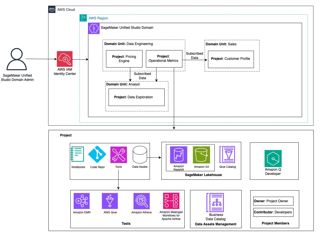
SageMaker Unified Studio facilitates collaboration among data scientists, analysts, engineers, and developers as they work on data, analytics, AI workflows, and applications. It provides familiar tools from AWS analytics and artificial intelligence and machine learning (AI/ML) services, including data processing, SQL analytics, ML model development, and generative AI application development, into a single user experience.

SageMaker Unified Studio

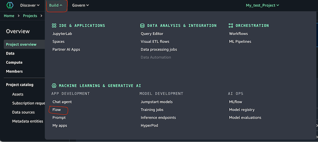
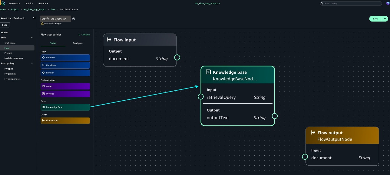
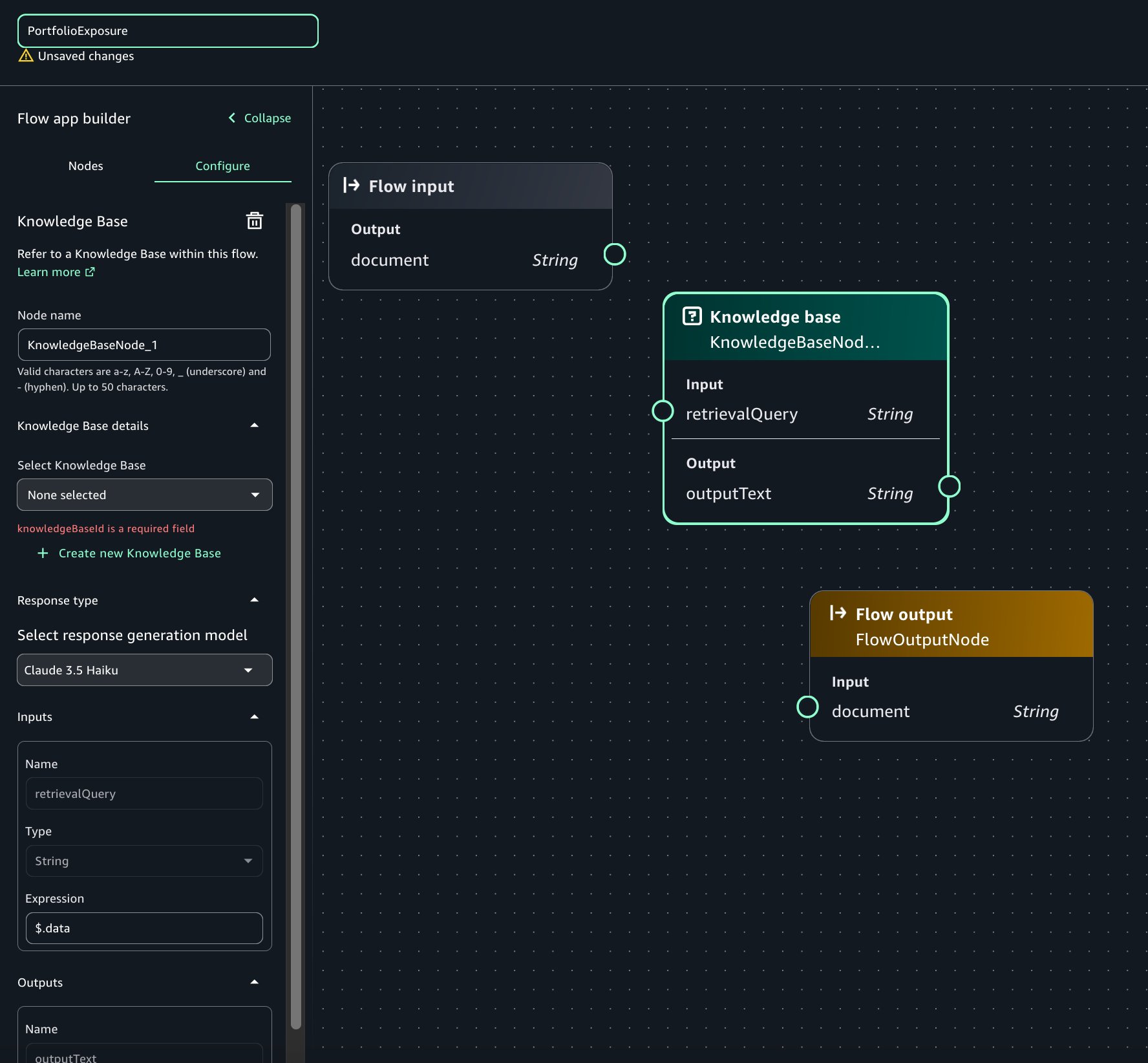
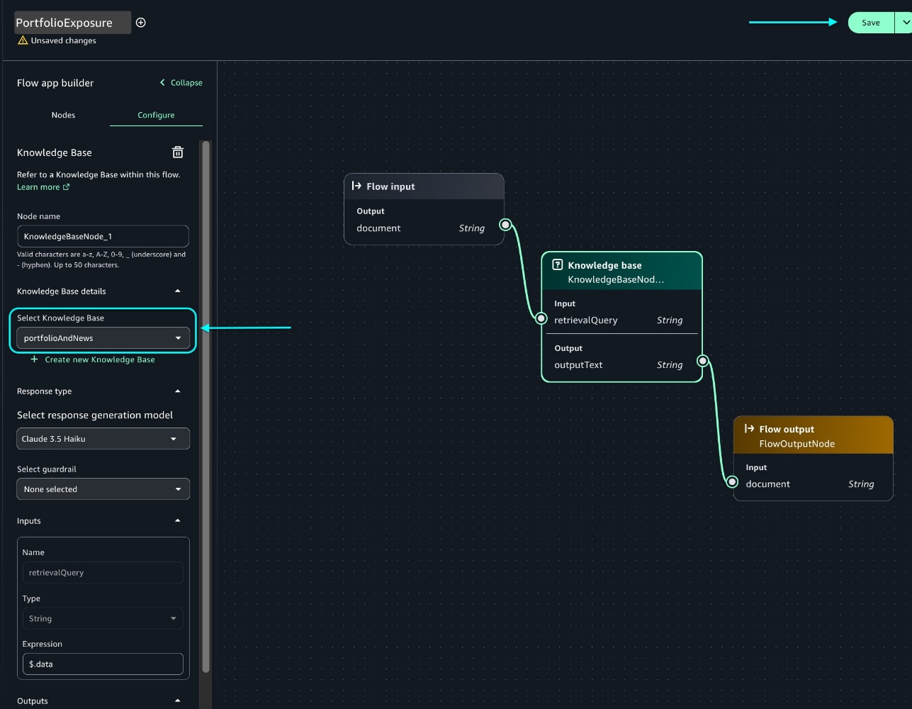
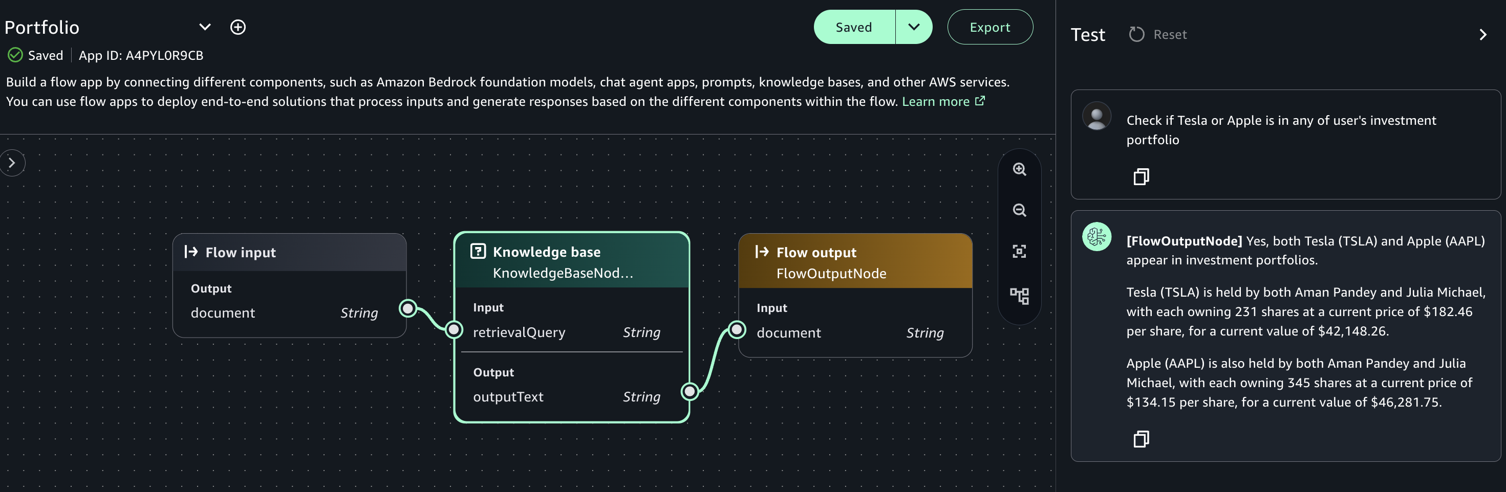
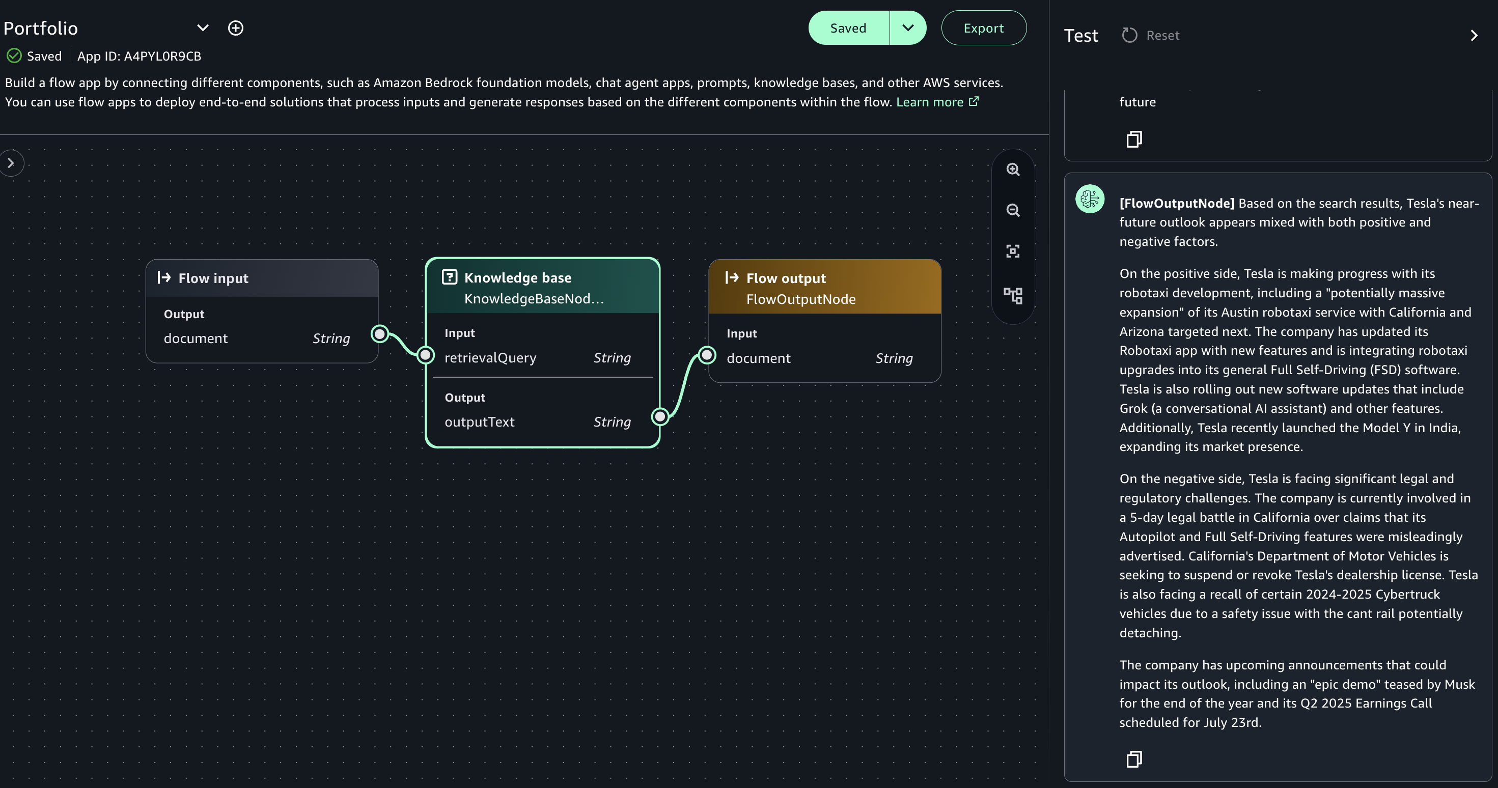
SageMaker Unified Studio also brings selected capabilities from Amazon Bedrock into SageMaker. You can now rapidly prototype, customize, and share generative AI applications using foundation models (FMs) and advanced features such as Amazon Bedrock Knowledge BasesAmazon Bedrock Guardrails, Amazon Bedrock Agents, and Amazon Bedrock Flows to create tailored solutions aligned with your requirements and responsible AI guidelines all within SageMaker.

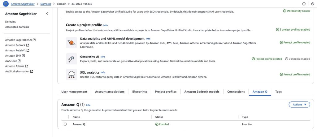
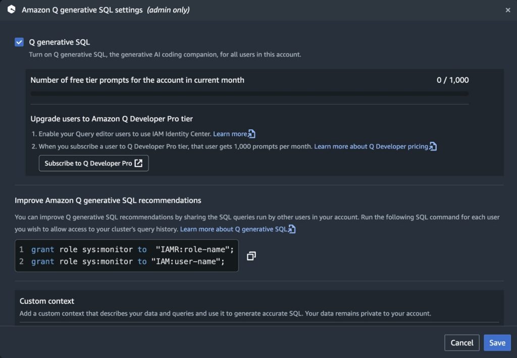
Last but not least, Amazon Q Developer is now generally available in SageMaker Unified Studio. Amazon Q Developer provides generative AI powered assistance for data and AI development. It helps you with tasks like writing SQL queries, building extract, transform, and load (ETL) jobs, and troubleshooting, and is available in the Free tier and Pro tier for existing subscribers.

You can learn more about SageMaker Unified Studio in this recent blog post written by my colleague Donnie.

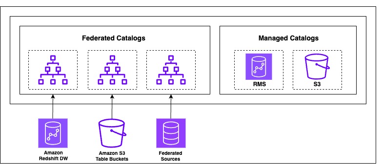
During re:Invent 2024, we also launched Amazon SageMaker Lakehouse as part of the next generation of SageMaker. SageMaker Lakehouse unifies all your data across Amazon S3 data lakes, Amazon Redshift data warehouses, and third-party and federated data sources. It helps you build powerful analytics and AI/ML applications on a single copy of your data. SageMaker Lakehouse gives you the flexibility to access and query your data in-place with Apache Iceberg–compatible tools and engines. In addition, zero-ETL integrations automate the process of bringing data into SageMaker Lakehouse from AWS data sources such as Amazon Aurora or Amazon DynamoDB and from applications such as Salesforce, Facebook Ads, Instagram Ads, ServiceNow, SAP, Zendesk, and Zoho CRM. The full list of integrations is available in the SageMaker Lakehouse FAQ.

Building a data foundation with Amazon S3
Building a data foundation is the cornerstone of accelerating analytics and AI workloads, enabling organizations to seamlessly manage, discover, and utilize their data assets at any scale. Amazon S3 is the world’s best place to build a data lake, with virtually unlimited scale, and it provides the essential foundation for this transformation.

I’m always astonished to learn about the scale at which we operate Amazon S3: It currently holds over 400 trillion objects, exabytes of data, and processes a mind-blowing 150 million requests per second. Just a decade ago, not even 100 customers were storing more than a petabyte (PB) of data on S3. Today, thousands of customers have surpassed the 1 PB milestone.

Amazon S3 stores exabytes of tabular data, and it averages over 15 million requests to tabular data per second. To help you reduce the undifferentiated heavy lifting when managing your tabular data in S3 buckets, we announced Amazon S3 Tables at AWS re:Invent 2024. S3 Tables are the first cloud object store with built-in support for Apache Iceberg. S3 tables are specifically optimized for analytics workloads, resulting in up to threefold faster query throughput and up to tenfold higher transactions per second compared to self-managed tables.

Today, we’re announcing the general availability of Amazon S3 Tables integration with Amazon SageMaker Lakehouse  Amazon S3 Tables now integrate with Amazon SageMaker Lakehouse, making it easy for you to access S3 Tables from AWS analytics services such as Amazon Redshift, Amazon Athena, Amazon EMR, AWS Glue, and Apache Iceberg–compatible engines such as Apache Spark or PyIceberg. SageMaker Lakehouse enables centralized management of fine-grained data access permissions for S3 Tables and other sources and consistently applies them across all engines.

For those of you who use a third-party catalog, have a custom catalog implementation, or only need basic read and write access to tabular data in a single table bucket, we’ve added new APIs that are compatible with the Iceberg REST Catalog standard. This enables any Iceberg-compatible application to seamlessly create, update, list, and delete tables in an S3 table bucket. For unified data management across all of your tabular data, data governance, and fine-grained access controls, you can also use S3 Tables with SageMaker Lakehouse.

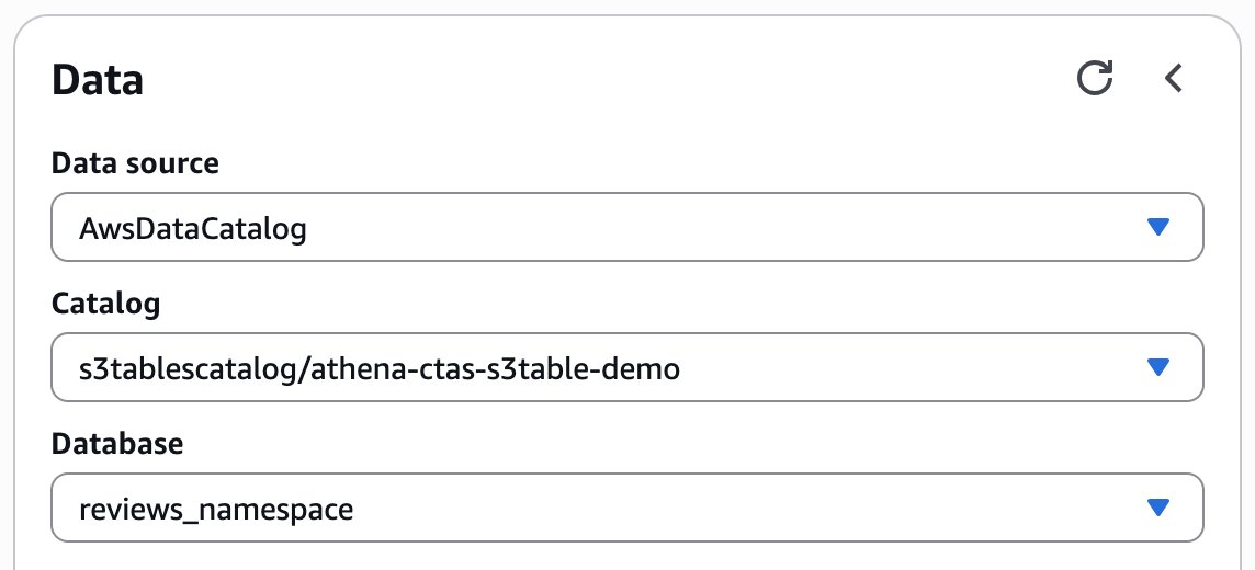
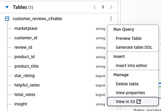
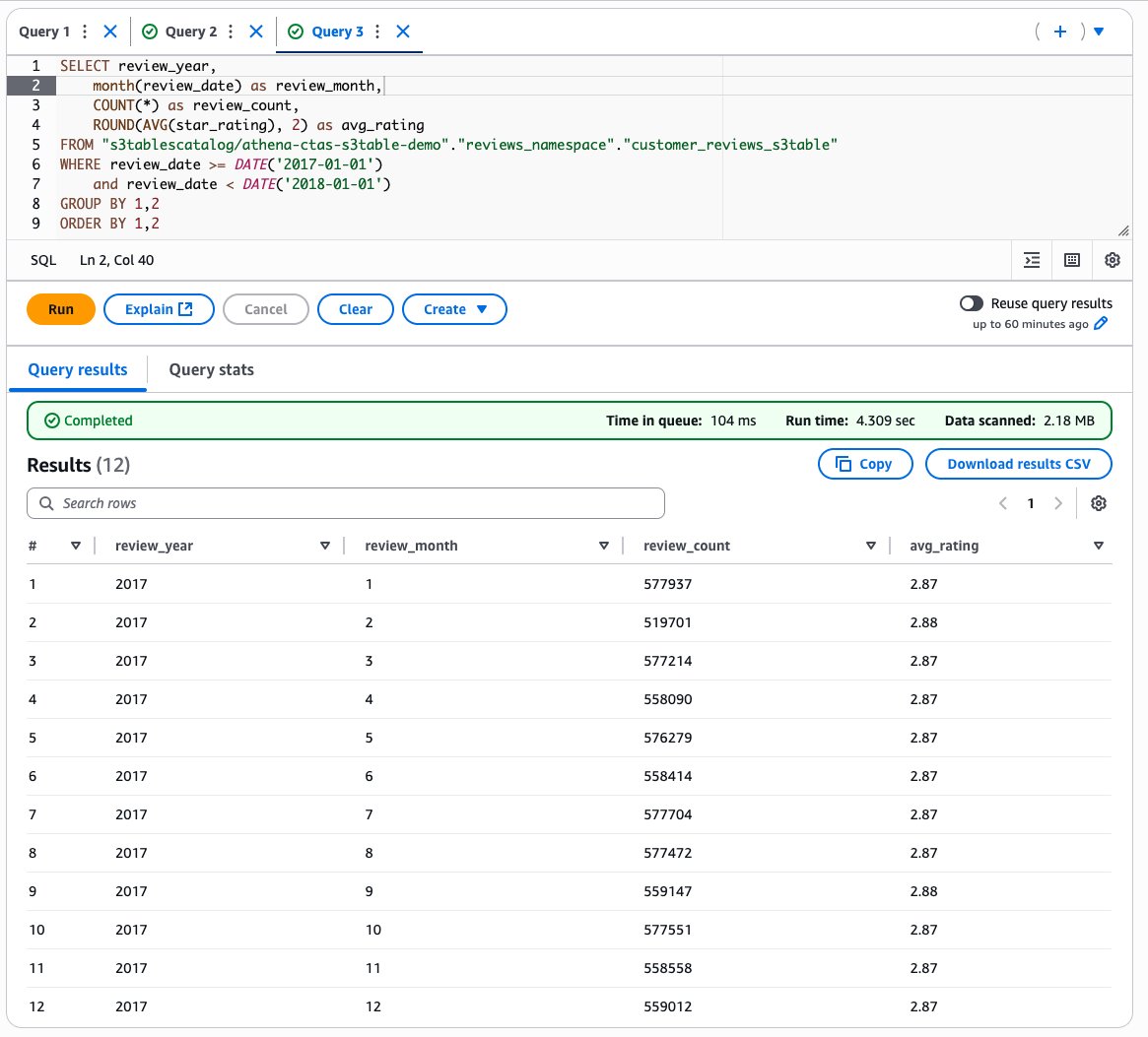
To help you access S3 Tables, we’ve launched updates in the AWS Management Console. You can now create a table, populate it with data, and query it directly from the S3 console using Amazon Athena, making it easier to get started and analyze data in S3 table buckets.

The following screenshot shows how to access Athena directly from the S3 console.

S3 console : create table with AthenaWhen I select Query tables with Athena or Create table with Athena, it opens the Athena console on the correct data source, catalog, and database.

S3 Tables in Athena

Since re:Invent 2024, we’ve continued to add new capabilities to S3 Tables at a rapid pace. For example, we added schema definition support to the CreateTable API and you can now create up to 10,000 tables in an S3 table bucket. We also launched S3 Tables into eight additional AWS Regions, with the most recent being Asia Pacific (Seoul, Singapore, Sydney) on March 4, with more to come. You can refer to the S3 Tables AWS Regions page of the documentation to get the list of the eleven Regions where S3 Tables are available today.

Amazon S3 Metadataannounced during re:Invent 2024— has been generally available since January 27. It’s the fastest and easiest way to help you discover and understand your S3 data with automated, effortlessly-queried metadata that updates in near real time. S3 Metadata works with S3 object tags. Tags help you logically group data for a variety of reasons, such as to apply IAM policies to provide fine-grained access, specify tag-based filters to manage object lifecycle rules, and selectively replicate data to another Region. In Regions where S3 Metadata is available, you can capture and query custom metadata that is stored as object tags. To reduce the cost associated with object tags when using S3 Metadata, Amazon S3 reduced pricing for S3 object tagging by 35 percent in all Regions, making it cheaper to use custom metadata.

AWS Pi Day 2025
Over the years, AWS Pi Day has showcased major milestones in cloud storage and data analytics. This year, the AWS Pi Day virtual event will feature a range of topics designed for developers and technical decision-makers, data engineers, AI/ML practitioners, and IT leaders. Key highlights include deep dives, live demos, and expert sessions on all the services and capabilities I discussed in this post.

By attending this event, you’ll learn how you can accelerate your analytics and AI innovation. You’ll learn how you can use S3 Tables with native Apache Iceberg support and S3 Metadata to build scalable data lakes that serve both traditional analytics and emerging AI/ML workloads. You’ll also discover the next generation of Amazon SageMaker, the center for all your data, analytics, and AI, to help your teams collaborate and build faster from a unified studio, using familiar AWS tools with access to all your data whether it’s stored in data lakes, data warehouses, or third-party or federated data sources.

For those looking to stay ahead of the latest cloud trends, AWS Pi Day 2025 is an event you can’t miss. Whether you’re building data lakehouses, training AI models, building generative AI applications, or optimizing analytics workloads, the insights shared will help you maximize the value of your data.

Tune in today and explore the latest in cloud data innovation. Don’t miss the opportunity to engage with AWS experts, partners, and customers shaping the future of data, analytics, and AI.

If you missed the virtual event on March 14, you can visit the event page at any time—we will keep all the content available on-demand there!

— seb


How is the News Blog doing? Take this 1 minute survey!

(This survey is hosted by an external company. AWS handles your information as described in the AWS Privacy Notice. AWS will own the data gathered via this survey and will not share the information collected with survey respondents.)

Accelerate analytics and AI innovation with the next generation of Amazon SageMaker

Post Syndicated from G2 Krishnamoorthy original https://aws.amazon.com/blogs/big-data/accelerate-analytics-and-ai-innovation-with-the-next-generation-of-amazon-sagemaker/

At AWS re:Invent 2024, we announced the next generation of Amazon SageMaker, the center for all your data, analytics, and AI. Amazon SageMaker brings together widely adopted AWS machine learning (ML) and analytics capabilities and addresses the challenges of harnessing organizational data for analytics and AI through unified access to tools and data with governance built in. It enables teams to securely find, prepare, and collaborate on data assets and build analytics and AI applications through a single experience, accelerating the path from data to value.

At the core of the next generation of Amazon SageMaker is Amazon SageMaker Unified Studio, a single data and AI development environment where you can find and access your organization’s data and act on it using the best tool for the job across virtually any use case. We are excited to announce the general availability of SageMaker Unified Studio.

In this post, we explore the benefits of SageMaker Unified Studio and how to get started.

Benefits of SageMaker Unified Studio

SageMaker Unified Studio brings together the functionality and tools from existing AWS Analytics and AI/ML services, including Amazon EMR, AWS Glue, Amazon Athena, Amazon Redshift, Amazon Bedrock, and Amazon SageMaker AI. From within the unified studio, you can discover data and AI assets from across your organization, then work together in projects to securely build and share analytics and AI artifacts, including data, models, and generative AI applications. Governance features including fine-grained access control are built into SageMaker Unified Studio using Amazon SageMaker Catalog to help you meet enterprise security requirements across your entire data estate.

Unified access to your data is provided by Amazon SageMaker Lakehouse, a unified, open, and secure data lakehouse built on Apache Iceberg open standards. Whether your data is stored in Amazon Simple Storage Service (Amazon S3) data lakes, Redshift data warehouses, or third-party and federated data sources, you can access it from one place and use it with Iceberg-compatible engines and tools. In addition, SageMaker Lakehouse now integrates with Amazon S3 Tables, the first cloud object store with native Apache Iceberg support, so you can use SageMaker Lakehouse to create, query, and process S3 Tables efficiently using various analytics engines in SageMaker Unified Studio as well as Iceberg-compatible engines like Apache Spark and PyIceberg.

Capabilities from Amazon Bedrock are now generally available in SageMaker Unified Studio, allowing you to rapidly prototype, customize, and share generative AI applications in a governed environment. Users have an intuitive interface to access high-performing foundation models (FMs) in Amazon Bedrock, including the Amazon Nova model series, and the ability to create Agents, Flows, Knowledge Bases, and Guardrails with a few clicks.

Amazon Q Developer, the most capable generative AI assistant for software development, can be used within SageMaker Unified Studio to streamline tasks across the data and AI development lifecycle, including code authoring, SQL generation, data discovery, and troubleshooting.

A new integrated way of working

The general availability of SageMaker Unified Studio represents another meaningful step in our journey to offer our customers a streamlined way to work with their data, whether for analytics or AI. Many of our customers have told us that you are building data-driven applications to guide business decisions, improve agility, and drive innovation, but that these applications are complex to build because they require collaboration across teams and the integration of data and tools. Not only is it time consuming for users to learn multiple development experiences, but because data, code, and other development artifacts are stored separately, it is challenging for users to understand how they interact with each other and to use them cohesively. Configuring and governing access is also a cumbersome manual process. To overcome these hurdles, many organizations are building bespoke integrations between services, tools, and homegrown access management systems. However, what you need is the flexibility to adopt the best services for your use case while empowering your data teams with a unified development experience.

“When we build data-driven applications for our customers, we want a unified platform where the technologies work together in an integrated way. Amazon SageMaker Unified Studio streamlines our solution delivery processes through comprehensive analytics capabilities, a unified studio experience, and a lakehouse that integrates data management across data warehouses and data lakes. Amazon SageMaker Unified Studio reduces the time-to-value for our customers’ data projects by up to 40%, helping us with our mission to accelerate our customers’ digital transformation journey.”

—Akihiro Suzue, Head of Solutions Sector, NTT DATA; Yuji Shono, Senior Manager, Apps & Data Technology Department, NTT DATA; Yuki Saito, Manager, Digital Success Solutions Division, NTT DATA

Millions of organizations trust AWS and utilize our comprehensive set of purpose-built analytics, AI/ML, and generative AI capabilities to power data-driven applications without compromising on performance, scale, or cost. Our goal for the next generation of Amazon SageMaker, including SageMaker Unified Studio, is to make data and AI workers more productive by providing access to all your data and tools in a single development environment.

Building from a single data and AI development environment

Let’s explore a common business challenge: increasing revenue through better lead generation. Consider an organization implementing an intelligent digital assistant on their website to engage with customers—a process that traditionally requires multiple tools and data sources. With SageMaker Unified Studio, this entire process can now be carried out within a single data and AI development environment.

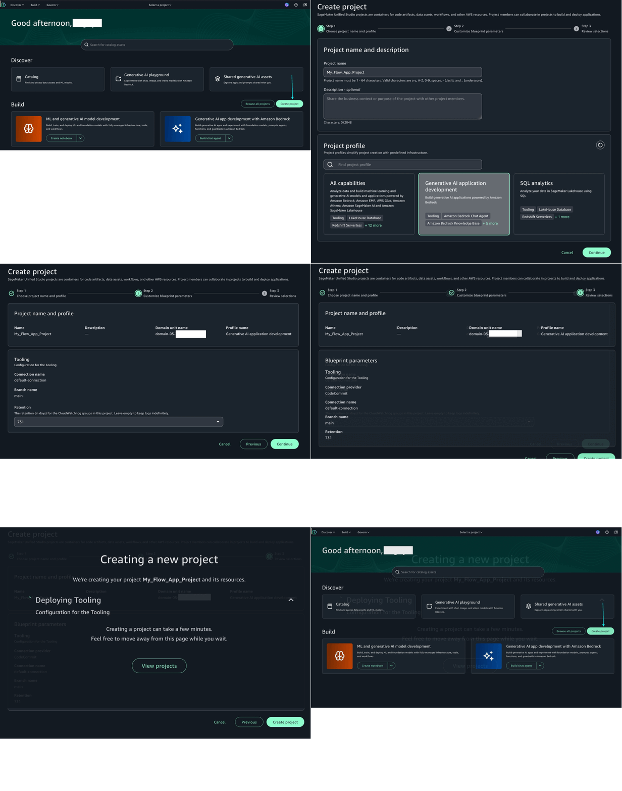
First, the data team uses the generative AI playground within SageMaker Unified Studio to quickly evaluate and select the best model for their customer interactions. They then create a project to house the tools and resources necessary for their use case and use Amazon Bedrock within the project to build and deploy a sophisticated virtual assistant that quickly begins qualifying leads through their website.

To identify the most promising opportunities, the team develops a segmentation strategy. The data engineer asks Amazon Q Developer to identify datasets that contain lead data and uses zero-ETL integrations to bring the data into SageMaker Lakehouse. The data analyst then discovers it and creates a comprehensive view of their market. They use the SQL query editor to build out marketing segments, which they then write back to SageMaker Lakehouse, where they are available to other team members.

Finally, the data scientist accesses the same dataset, which they use to train and deploy an automated lead scoring model using tools available from SageMaker AI. During the model development phase, they use Amazon Q Developer’s inline code authoring and troubleshooting capabilities to efficiently write error free-code in their JupyterLab notebook. The final model provides sales teams with the highest-value opportunities, which they can visualize in a business intelligence dashboard and take action on immediately.

Reducing time-to-value in a unified environment

What is remarkable about this example is that entire process happens in one integrated environment. Without SageMaker Unified Studio, the team would have had to work with multiple data sources, tools, and services, spending time learning multiple development environments, creating resources shares, and manually configuring access controls. The data engineer and data analyst would have worked in various data warehouses, data lakes, and analytics tools, the data scientist would have worked in an ML studio and notebook environment, and the application builder in a generative AI tool. Now, they’re able to build and collaborate with their data and tools available in one experience, dramatically reducing time-to-value.

That’s why we’re so excited about the next generation of Amazon SageMaker and the general availability of SageMaker Unified Studio. We believe that by putting everything you need for analytics and AI in one place, you can solve complex end-to-end problems more efficiently and get to innovative outcomes faster than ever before.

Getting started with SageMaker Unified Studio

To learn more, check out the following resources:


About the authors

G2 Krishnamoorthy is VP of Analytics, leading AWS data lake services, data integration, Amazon OpenSearch Service, and Amazon QuickSight. Prior to his current role, G2 built and ran the Analytics and ML Platform at Facebook/Meta, and built various parts of the SQL Server database, Azure Analytics, and Azure ML at Microsoft.

Rahul Pathak is VP of Relational Database Engines, leading Amazon Aurora, Amazon Redshift, and Amazon QLDB. Prior to his current role, he was VP of Analytics at AWS, where he worked across the entire AWS database portfolio. He has co-founded two companies, one focused on digital media analytics and the other on IP-geolocation.

Collaborate and build faster with Amazon SageMaker Unified Studio, now generally available

Post Syndicated from Donnie Prakoso original https://aws.amazon.com/blogs/aws/collaborate-and-build-faster-with-amazon-sagemaker-unified-studio-now-generally-available/

Today, we’re announcing the general availability of Amazon SageMaker Unified Studio, a single data and AI development environment where you can find and access all of the data in your organization and act on it using the best tool for the job across virtually any use case. Introduced as preview during AWS re:Invent 2024, my colleague, Antje, summarized it as:

SageMaker Unified Studio (preview) is a single data and AI development environment. It brings together functionality and tools from the range of standalone “studios,” query editors, and visual tools that we have today in Amazon AthenaAmazon EMRAWS GlueAmazon RedshiftAmazon Managed Workflows for Apache Airflow (Amazon MWAA), and the existing SageMaker Studio.

Here’s a video to see Amazon SageMaker Unified Studio in action:

SageMaker Unified Studio breaks down silos in data and tools, giving data engineers, data scientists, data analysts, ML developers and other data practitioners a single development experience. This saves development time and simplifies access control management so data practitioners can focus on what really matters to them—building data products and AI applications.

This post focuses on several important announcements that we’re excited to share:

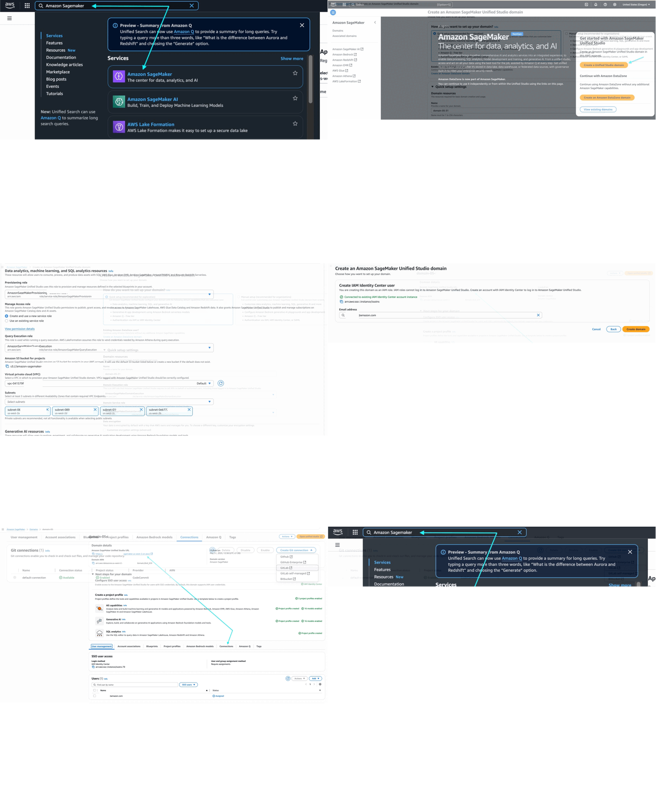
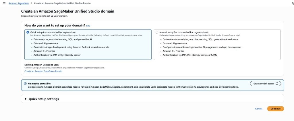
To get started, go to the Amazon SageMaker console and create a SageMaker Unified Studio domain. To learn more, visit Create an Amazon SageMaker Unified Studio domain in the AWS documentation.

New capabilities for Amazon Bedrock in SageMaker Unified Studio
The capabilities of Amazon Bedrock within Amazon SageMaker Unified Studio offer a governed collaborative environment for developers to rapidly create and customize generative AI applications. This intuitive interface caters to developers of all skill levels, providing seamless access to the high-performance FMs offered in Amazon Bedrock and advanced customization tools for collaborative development of tailored generative AI applications.

Since the preview launch, several new FMs have become available in Amazon Bedrock and are fully integrated with SageMaker Unified Studio, including Anthropic’s Claude 3.7 Sonnet and DeepSeek-R1. These models can be used for building generative AI apps and chatting in the playground in SageMaker Unified Studio.

Here’s how you can choose Anthropic’s Claude 3.7 Sonnet on the model selection in your project.

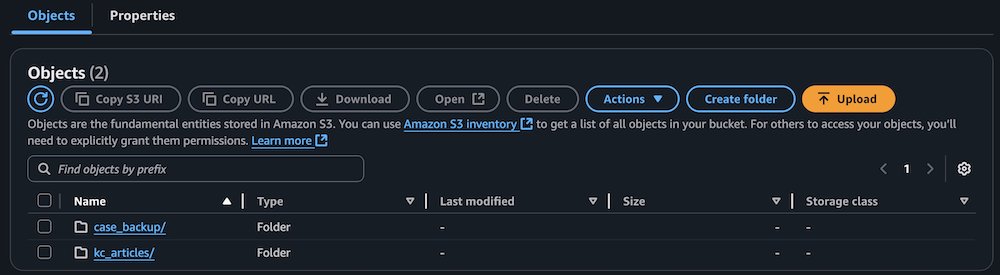
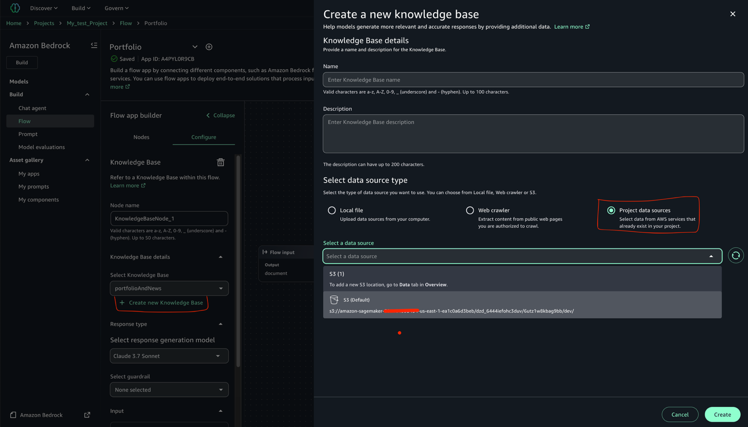
You can also source data or documents from S3 folders within your project and select specific FMs when creating knowledge bases. 

During preview, we introduced Amazon Bedrock Guardrails to help you implement safeguards for your Amazon Bedrock application based on your use cases and responsible AI policies. Now, Amazon Bedrock Guardrails is extended to Amazon Bedrock Flows with this general availability release.

Additionally, we have streamlined generative AI setup for associated accounts with a new user management interface in SageMaker Unified Studio, making it straightforward for domain administrators to grant associated account admins access to model governance projects. This enhancement eliminates the need for command line operations, streamlining the process of configuring generative AI capabilities across multiple AWS accounts.

These new features eliminate barriers between data, tools, and builders in the generative AI development process. You and your team will gain a unified development experience by incorporating the powerful generative AI capabilities of Amazon Bedrock — all within the same workspace.

Amazon Q Developer is now generally available in SageMaker Unified Studio
Amazon Q Developer is now generally available in Amazon SageMaker Unified Studio, providing data professionals with generative AI–powered assistance across the entire data and AI development lifecycle.

Amazon Q Developer integrates with the full suite of AWS analytics and AI/ML tools and services within SageMaker Unified Studio, including data processing, SQL analytics, machine learning model development, and generative AI application development, to accelerate collaboration and help teams build data and AI products faster. To get started, you can select Amazon Q Developer icon.

For new users of SageMaker Unified Studio, Amazon Q Developer serves as an invaluable onboarding assistant. It can explain core concepts such as domains and projects, provide guidance on setting up environments, and answer your questions.

Amazon Q Developer helps you discover and understand data using powerful natural language interactions with SageMaker Catalog. What makes this implementation particularly powerful is how Amazon Q Developer combines broad knowledge of AWS analytics and AI/ML services with the user’s context to provide personalized guidance.

You can chat about your data assets through a conversational interface, asking questions such as “Show all payment related datasets” without needing to navigate complex metadata structures.

Amazon Q Developer offers SQL query generation through its integration with the built-in query editor available in SageMaker Unified Studio. Data professionals of varying skill levels can now express their analytical needs in natural language, receiving properly formatted SQL queries in return.

For example, you can ask, “Analyze payment method preferences by age group and region” and Amazon Q Developer will generate the appropriate SQL with proper joins across multiple tables.

Additionally, Amazon Q Developer is also available to assist with troubleshooting and generating real-time code suggestions in SageMaker Unified Studio Jupyter notebooks, as well as building ETL jobs.

Now available

  • Availability — Amazon SageMaker Unified Studio is now available in the following AWS Regions: US East (N. Virginia, Ohio), US West (Oregon), Asia Pacific (Seoul, Singapore, Sydney, Tokyo), Canada (Central), Europe (Frankfurt, Ireland, London), South America (São Paulo). Learn more about the availability of these capabilities on supported Region documentation page.
  • Amazon Q Developer subscription — The free tier of Amazon Q Developer is available by default in SageMaker Unified Studio, requiring no additional setup or configuration. If you already have Amazon Q Developer Pro Tier subscriptions, you can use those enhanced capabilities within the SageMaker Unified Studio environment. For more information, visit the documentation page.
  • Amazon Bedrock capabilities — To learn more about the capabilities of Amazon Bedrock in Amazon SageMaker Unified Studio, refer to this documentation page

Start building with Amazon SageMaker Unified Studio today. For more information, visit the Amazon SageMaker Unified Studio page.

Happy building!

Donnie Prakoso

— How is the News Blog doing? Take this 1 minute survey! (This survey is hosted by an external company. AWS handles your information as described in the AWS Privacy Notice. AWS will own the data gathered via this survey and will not share the information collected with survey respondents.)

Amazon S3 Tables integration with Amazon SageMaker Lakehouse is now generally available

Post Syndicated from Channy Yun (윤석찬) original https://aws.amazon.com/blogs/aws/amazon-s3-tables-integration-with-amazon-sagemaker-lakehouse-is-now-generally-available/

At re:Invent 2024, we launched Amazon S3 Tables, the first cloud object store with built-in Apache Iceberg support to streamline storing tabular data at scale, and Amazon SageMaker Lakehouse to simplify analytics and AI with a unified, open, and secure data lakehouse. We also previewed S3 Tables integration with Amazon Web Services (AWS) analytics services for you to stream, query, and visualize S3 Tables data using Amazon Athena, Amazon Data Firehose, Amazon EMR, AWS Glue, Amazon Redshift, and Amazon QuickSight.

Our customers wanted to simplify the management and optimization of their Apache Iceberg storage, which led to the development of S3 Tables. They were simultaneously working to break down data silos that impede analytics collaboration and insight generation using the SageMaker Lakehouse. When paired with S3 Tables and SageMaker Lakehouse in addition to built-in integration with AWS analytics services, they can gain a comprehensive platform unifying access to multiple data sources enabling both analytics and machine learning (ML) workflows.

Today, we’re announcing the general availability of Amazon S3 Tables integration with Amazon SageMaker Lakehouse to provide unified S3 Tables data access across various analytics engines and tools. You can access SageMaker Lakehouse from Amazon SageMaker Unified Studio, a single data and AI development environment that brings together functionality and tools from AWS analytics and AI/ML services. All S3 tables data integrated with SageMaker Lakehouse can be queried from SageMaker Unified Studio and engines such as Amazon Athena, Amazon EMR, Amazon Redshift, and Apache Iceberg-compatible engines like Apache Spark or PyIceberg.

With this integration, you can simplify building secure analytic workflows where you can read and write to S3 Tables and join with data in Amazon Redshift data warehouses and third-party and federated data sources, such as Amazon DynamoDB or PostgreSQL.

You can also centrally set up and manage fine-grained access permissions on the data in S3 Tables along with other data in the SageMaker Lakehouse and consistently apply them across all analytics and query engines.

S3 Tables integration with SageMaker Lakehouse in action
To get started, go to the Amazon S3 console and choose Table buckets from the navigation pane and select Enable integration to access table buckets from AWS analytics services.

Now you can create your table bucket to integrate with SageMaker Lakehouse. To learn more, visit Getting started with S3 Tables in the AWS documentation.

1. Create a table with Amazon Athena in the Amazon S3 console
You can create a table, populate it with data, and query it directly from the Amazon S3 console using Amazon Athena with just a few steps. Select a table bucket and select Create table with Athena, or you can select an existing table and select Query table with Athena.

2. Create tables with Athena

When you want to create a table with Athena, you should first specify a namespace for your table. The namespace in an S3 table bucket is equivalent to a database in AWS Glue, and you use the table namespace as the database in your Athena queries.

Choose a namespace and select Create table with Athena. It goes to the Query editor in the Athena console. You can create a table in your S3 table bucket or query data in the table.

2. Query with Athena

2. Query with SageMaker Lakehouse in the SageMaker Unified Studio
Now you can access unified data across S3 data lakes, Redshift data warehouses, third-party and federated data sources in SageMaker Lakehouse directly from SageMaker Unified Studio.

To get started, go to the SageMaker console and create a SageMaker Unified Studio domain and project using a sample project profile: Data Analytics and AI-ML model development. To learn more, visit Create an Amazon SageMaker Unified Studio domain in the AWS documentation.

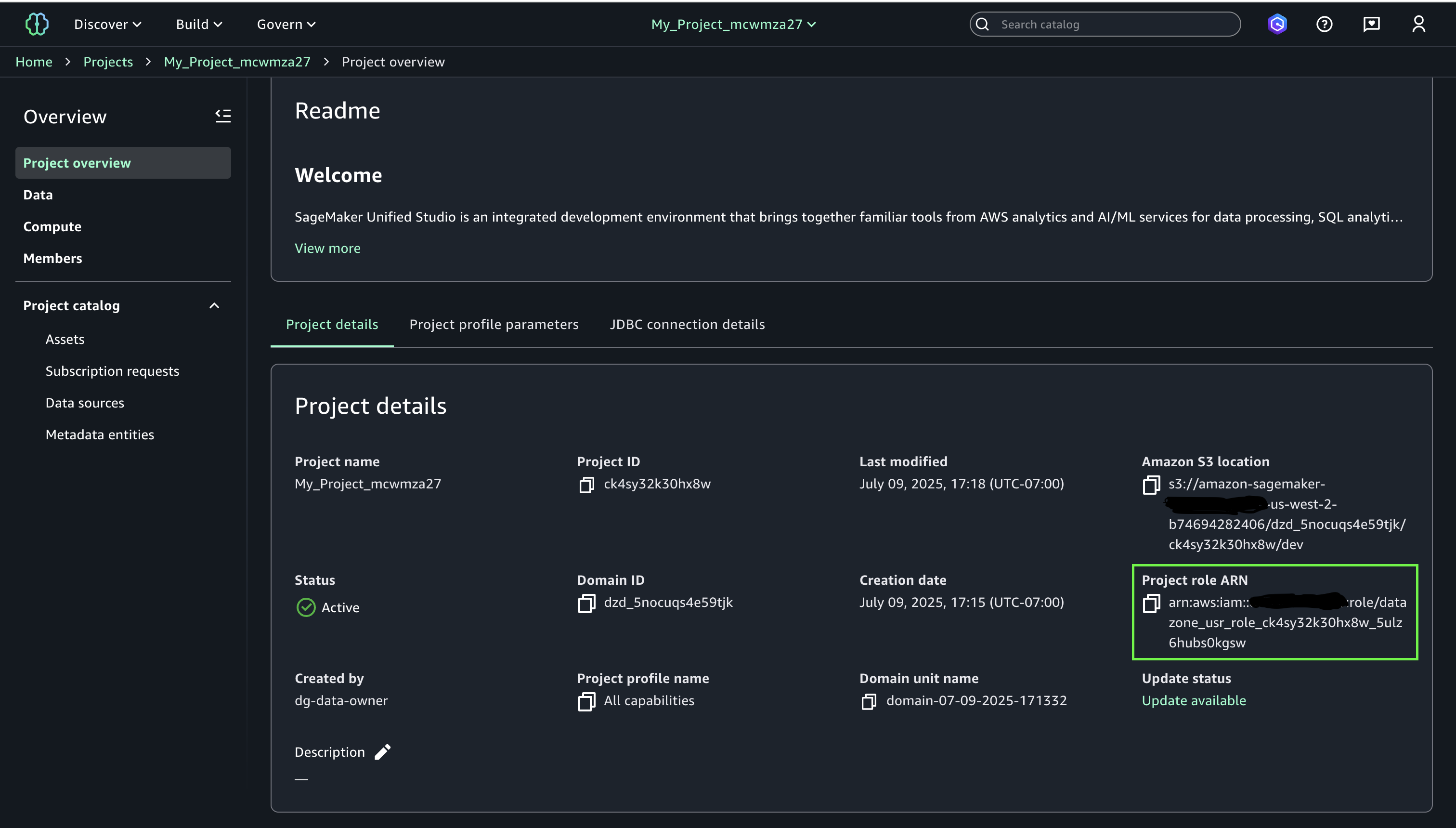
After the project is created, navigate to the project overview and scroll down to project details to note down the project role Amazon Resource Name (ARN).

3. Project details in SageMaker Unified Studio

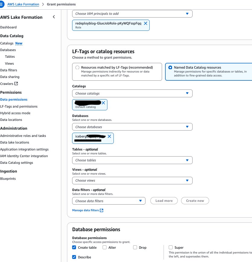
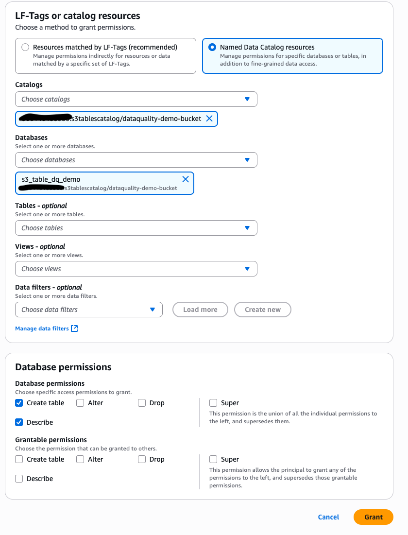
Go to the AWS Lake Formation console and grant permissions for AWS Identity and Access Management (IAM) users and roles. In the in the Principals section, select the <project role ARN> noted in the previous paragraph. Choose Named Data Catalog resources in the LF-Tags or catalog resources section and select the table bucket name you created for Catalogs. To learn more, visit Overview of Lake Formation permissions in the AWS documentation.

4. Grant permissions in Lake Formation console

When you return to SageMaker Unified Studio, you can see your table bucket project under Lakehouse in the Data menu in the left navigation pane of project page. When you choose Actions, you can select how to query your table bucket data in Amazon Athena, Amazon Redshift, or JupyterLab Notebook.

5. S3 Tables in Unified Studio

When you choose Query with Athena, it automatically goes to Query Editor to run data query language (DQL) and data manipulation language (DML) queries on S3 tables using Athena.

Here is a sample query using Athena:

select * from "s3tablecatalog/s3tables-integblog-bucket”.”proddb"."customer" limit 10;

6. Athena query in Unified Studio

To query with Amazon Redshift, you should set up Amazon Redshift Serverless compute resources for data query analysis. And then you choose Query with Redshift and run SQL in the Query Editor. If you want to use JupyterLab Notebook, you should create a new JupyterLab space in Amazon EMR Serverless.

3. Join data from other sources with S3 Tables data
With S3 Tables data now available in SageMaker Lakehouse, you can join it with data from data warehouses, online transaction processing (OLTP) sources like relational or non-relational database, Iceberg tables, and other third party sources to gain more comprehensive and deeper insights.

For example, you can add connections to data sources such as Amazon DocumentDB, Amazon DynamoDB, Amazon Redshift, PostgreSQL, MySQL, Google BigQuery, or Snowflake and combine data using SQL without extract, transform, and load (ETL) scripts.

Now you can run the SQL query in the Query editor to join the data in the S3 Tables with the data in the DynamoDB.

Here is a sample query to join between Athena and DynamoDB:

select * from "s3tablescatalog/s3tables-integblog-bucket"."blogdb"."customer", 
              "dynamodb1"."default"."customer_ddb" where cust_id=pid limit 10;

To learn more about this integration, visit Amazon S3 Tables integration with Amazon SageMaker Lakehouse in the AWS documentation.

Now available
S3 Tables integration with SageMaker Lakehouse is now generally available in all AWS Regions where S3 Tables are available. To learn more, visit the S3 Tables product page and the SageMaker Lakehouse page.

Give S3 Tables a try in the SageMaker Unified Studio today and send feedback to AWS re:Post for Amazon S3 and AWS re:Post for Amazon SageMaker or through your usual AWS Support contacts.

In the annual celebration of the launch of Amazon S3, we will introduce more awesome launches for Amazon S3 and Amazon SageMaker. To learn more, join the AWS Pi Day event on March 14.

Channy

How is the News Blog doing? Take this 1 minute survey!

(This survey is hosted by an external company. AWS handles your information as described in the AWS Privacy Notice. AWS will own the data gathered via this survey and will not share the information collected with survey respondents.)

Enhancing Adobe Marketo Engage Data Analysis with AWS Glue Integration

Post Syndicated from Kenny Rajan original https://aws.amazon.com/blogs/big-data/enhancing-adobe-marketo-engage-data-analysis-with-aws-glue-integration/

Today’s digital-first, B2B landscape presents marketers with complex challenges as they navigate sophisticated buyer journeys involving diverse decision-making groups. Adobe Marketo Engage offers a comprehensive marketing hub for orchestrating cross-channel campaigns. Using AI-driven personalization, automation, and real-time analytics, it helps businesses acquire and retain customers throughout their buying journeys. Marketo Engage empowers B2B marketers to navigate modern complexities and successfully drive measurable business growth through multi-channel engagement, automated customer journeys, and sales-marketing collaboration.

To further enhance their B2B marketing capabilities, organizations are now looking to fully use their marketing data for more informed decision-making and strategy optimization. Recognizing the need to simplify the analytics pipeline, AWS introduced software as a service (SaaS) connectivity for Marketo Engage through AWS Glue, delivering insights faster to enable data-driven decisions. The agile, serverless nature of AWS Glue meets a range of data analytics needs while reducing costs. This powerful integration links the robust marketing automation features of Marketo Engage with AWS’s advanced analytics ecosystem. By seamlessly connecting the platforms, businesses can extract greater value from marketing data, gaining deeper insights into customer behavior and campaign performance. Together, AWS Glue and Marketo Engage unlock new possibilities for data-driven marketing:

  • Marketing-sales alignment – Helps automate the transfer of lead and opportunity data between Marketo Engage and CRM systems, making sure that sales and marketing teams are aligned and responsive to customer needs
  • Enhanced analytics – Connects Marketo Engage with business intelligence (BI) tools for data-driven campaign optimization, allowing marketers to extract meaningful insights and make informed decisions
  • Data integrity – Maintains consistent, high-quality data across all systems, providing reliability and accuracy in marketing and sales operations
  • Improved lead quality – Refines lead scoring processes by using the advanced analytics capabilities of AWS, resulting in better-qualified leads and improved sales conversions
  • Unified customer view – Provides comprehensive customer insights using enriched AWS datasets for Marketo Engage, offering a holistic understanding of customer interactions and behaviors

In this post, we show you how to use AWS Glue to extract data from Marketo Engage for data processing and enrichment on AWS for use in marketing analytics workflows.

Solution Overview

We explore a use case in which a company wants to run analysis for campaign leads in multiple countries. The resulting leads will be shared with the respective regional marketing representatives. The solution uses AWS Glue to extract data from Marketo Engage and save it in an Amazon Simple Storage Service (Amazon S3) bucket. The following diagram illustrates the solution architecture.

1_Scope-of-the-solutions_AWSGLue_Marketo_Engage_Flow

In the following sections, we walk through the high-level steps to implement the solution:

  1. Create AWS resources to connect to Marketo Engine and store data.
  2. Create an AWS Glue connection.
  3. Create an extract, transform, and load (ETL) job using AWS Glue Studio.
  4. Analyze the data.

Prerequisites

To set up the integration between Marketo Engage and AWS, the following components are required:

  • A Marketo Engage account – If you don’t already have one, create a Marketo Engage application and record the Munchkin ID, client ID, and client secret for the application. Refer to the Marketo Engage developer portal to set up the connection.
  • An AWS Glue database – This will serve as the data interaction interface on AWS. The database will expose the data residing in Amazon S3 as queryable AWS Glue tables. For this post, our database is called marketodb.

Create AWS resources to connect to Marketo Engage and store data

We use an AWS CloudFormation template to create an S3 bucket to store data, an AWS Secrets Manager secret for Marketo Engage that the AWS Glue connection needs, and an AWS Identity and Access Management (IAM) role to access the secret. Complete the following steps:

  1. Click Launch Stack below.
    Click here to launch the Cloud Fromation stack
  2. On the Specify stack details page, enter a name for the stack.
  3. Specify the Marketo client secret.
  4. Choose Next.
  5. On the Configure stack options page, choose Next.
  6. On the Review page, select I acknowledge that AWS CloudFormation might create IAM resources.
  7. Choose Submit. Note: The stack takes about 2 minutes to deploy.
  8. After the stack is created, make a note of the S3AccessRoleARN You will need this to create the Marketo Engage connection.

Create an AWS Glue connection

Complete the following steps to create an AWS Glue connection:

  1. On the AWS Glue console, choose Data connections in the navigation pane.
  2. Choose Create connection.
  3. For Data sources, select Marketo.

2-Glue-Data-Source-page

  1. Enter the Adobe MUNCHKIN_ID.
  2. Choose the IAM role created in the previous section as the AWS Glue connection IAM service role.
  3. Provide the Adobe ClientId as the user-managed client application client ID.
  4. Provide the Secrets Manager secret you created earlier.
  5. Choose Next.
  6. Specify your preferred connection name.
  7. Choose Next.
  8. Review the settings, then choose Create connection.

Entering-Marketo-Connectiondetails-in-glue.jpg

Create an ETL job using AWS Glue Studio

Complete the following steps to create an ETL job:

  1. On the AWS Glue console, choose ETL jobs in the navigation pane.
  2. Choose Create job.
  3. Choose Visual ETL.
  4. Add Marketo as a source node.
  5. Add Amazon S3 as the target node.
    Selecting Source Adobe Marketo Engage as Target and Amazon S3 as the target node in the AWS glue Visual Flow
  1. Choose the Marketo Engage data source node, and the editor will show a configuration pane on the right side of the diagram.
  2. In the Data source properties pane, provide the following information:
    1. For Name, enter a name (for example, Marketo).
    2. For Marketo connection, choose your Marketo Engage connection.
    3. For Entity Name, choose Leads as the entity to retrieve from Marketo Engage.
    4. For Fields, choose All Fields as the fields to retrieve from Marketo Engage.
    5. For Filter, enter gender=’Male’ to pull leads according to the campaign criteria. Note that in this blog post you’re using a synchronous mode in which the Marketo Adobe API limits require that the retrieved data set is less that 1000. See the AWS documentation to apply the criteria and mechanisms that support your campaigns.

You can observe the data preview pane reflecting the modifications you have made.

5-Entering-Marketo-Source-Properties-in-glue

  1. Choose the Amazon S3 target node to configure it.
  2. In the Data target properties pane, provide the following information:
    1. For Name, enter a name (for example, Amazon S3).
    2. For Node parents¸ choose Marketo.
    3. For Format, choose Parquet.
    4. For Compression Type¸ choose Snappy.
    5. For S3 Target Location, enter the path to the S3 bucket you created earlier, and optionally specify a prefix. This will inform the ETL job where to store the data retrieved from Marketo Engage.
    6. For Data Catalog update options, select Create a table in the Data Catalog and on subsequent runs, update the schema and add new partitions.
    7. For Database, choose your database in the AWS Glue Data Catalog.
    8. For Table name, enter a table name for the Data Catalog (for example, marketo_leads).

After you configure the source and target nodes, both nodes in the Visual ETL Editor should have a green check mark, indicating they are correctly configured.

  1. Specify the name for the job and save it.
  2. When the job is saved, choose Run to invoke the ETL job.
  3. After the job starts, go to the Runs tab and observe the run until completion.

Depending on the size of the data in your account object in Marketo Engage, the job will take a few minutes to complete. After a successful job run, a new table called marketo_leads is created and populated with data from Marketo Engage.

Analyze the data

After a successful run, you can now use Amazon Athena analyze the data from Marketo Engage with the data residing on AWS. If you’re using Athena for the first time, refer to Create a query output location for instructions to set up the query editor. Then run the following query:

SELECT country, COUNT(*) as count FROM marketo_leads GROUP BY country ORDER BY country;

The query will output the number of people within each country who can be contacted as targeting leads for campaigns, and you can enrich this output by adding other datasets in your data lake or data warehouse. You can expect to see an output like the following screenshot.

Executing Query to find campaign information using Marketo Engage data

Clean up

To avoid incurring charges, clean up the resources in your AWS account by completing the following steps:

  1. Delete the table created from the Data Catalog:
    1. On the AWS Glue console, navigate to the Data Catalog.
    2. Select the table and choose Delete.
  2. Delete the ETL job:
    1. On the AWS Glue console, choose ETL jobs in the navigation pane.
    2. From the list of jobs, select the job you created, and on the Actions menu, choose Delete.
  3. Delete the data connection:
    1. On the AWS Glue console, choose Data connections in the navigation pane.
    2. Select the Marketo Engage connection from the list of connectors, and on the Actions menu, choose Delete.
  4. Delete the CloudFormation stack:
    1. On the CloudFormation console, choose Stacks in the navigation pane.
    2. Select the stack you created for the S3 bucket and related resources and delete it.

Conclusion

The AWS Glue connector for Marketo Engage streamlines data integration, permitting seamless data synchronization between Marketo Engage and AWS services for a holistic view of customer information. This powerful integration enhances the capacity for advanced analytics, enabling marketers to glean precise and insightful learnings from their data; these insights can then be used to inform and refine marketing strategies, boosting campaign performance and driving better business outcomes

For more information on the AWS Glue connector for Marketo Engage and AWS Glue, refer to the relevant user guides and visit the AWS Glue website.


About the Authors

Kenny Rajan is a Principal Enterprise Architect at AWS specializing in integrating generative AI with enterprise systems like SAP and Adobe. He helps organizations modernize their digital experience platforms and supply chain and back-end systems through data and AI-powered cloud solutions. Outside of work, he contributes to technology education and charitable initiatives.

Author Rafael Profile PictureRafał Pawłaszek is a Senior Cloud Application Architect at AWS. Rafał supports customer transformation to the cloud and customer enablement in the cloud. Outside of work, he is interested in astronomy, astrophysics, and psychology, and loves spending time with family.

Author Basher Profile PictureBasheer Sheriff is a Senior Solutions Architect at AWS. He loves to help customers solve interesting problems using new technology. He is based in Melbourne, Australia, and likes to play sports such as football and cricket.

Author Kamen Profile PictureKamen Sharlandjiev is a Sr. Big Data Solutions Architect, Amazon MWAA and AWS Glue ETL expert. He’s on a mission to make life easier for customers who are facing complex data integration and orchestration challenges. His secret weapon? Fully managed AWS services that can get the job done with minimal effort. Follow Kamen on LinkedIn to keep up to date with the latest Amazon MWAA and AWS Glue features and news!

Unlock the power of optimization in Amazon Redshift Serverless

Post Syndicated from Ricardo Serafim original https://aws.amazon.com/blogs/big-data/unlock-the-power-of-optimization-in-amazon-redshift-serverless/

Amazon Redshift Serverless automatically scales compute capacity to match workload demands, measuring this capacity in Redshift Processing Units (RPUs). Although traditional scaling primarily responds to query queue times, the new AI-driven scaling and optimization feature offers a more sophisticated approach by considering multiple factors including query complexity and data volume. Intelligent scaling addresses key data warehouse challenges by preventing both over-provisioning of resources for performance and under-provisioning to save costs, particularly for workloads that fluctuate based on daily patterns or monthly cycles.

Amazon Redshift serverless now offers enhanced flexibility in configuring workgroups through two primary methods. Users can either set a base capacity, specifying the baseline RPUs for query execution, with options ranging from 8 to 1024 RPUs and each RPU providing 16 GB of memory, or they can opt for the price-performance target. Amazon Redshift Serverless AI-driven scaling and optimization can adapt more precisely to diverse workload requirements and employs intelligent resource management, automatically adjusting resources during query execution for optimal performance. Consider using AI-driven scaling and optimization if your current workload requires 32 to 512 base RPUs. We don’t recommend using this feature for less than 32 base RPU or more than 512 base RPU workloads.

In this post, we demonstrate how Amazon Redshift Serverless AI-driven scaling and optimization impacts performance and cost across different optimization profiles.

Options in AI-driven scaling and optimization

Amazon Redshift Serverless AI-driven scaling and optimization offers an intuitive slider interface, letting you balance price and performance goals. You can select from five optimization profiles, ranging from Optimized for Cost to Optimized for Performance, as shown in the following diagram. Your slider position determines how Amazon Redshift allocates resources and implements AI-driven scaling and optimizations, to achieve your desired price-performance target.

Sliding bar

The slider offers the following options:

  1. Optimized for Cost (1)
    • Prioritizes cost savings over performance
    • Allocates minimum resources in favor of saving on costs
    • Best for workloads where performance isn’t time-critical
  2. Cost-Balanced (25)
    • Balances towards cost savings while maintaining reasonable performance
    • Allocates moderate resources
    • Suitable for mixed workloads with some flexibility in query time
  3. Balanced (50)
    • Provides equal emphasis on cost efficiency and performance
    • Allocates optimal resources for most use cases
    • Ideal for general-purpose workloads
  4. Performance-Balanced (75)
    • Favors performance while maintaining some cost control
    • Allocates additional resources when needed
    • Suitable for workloads requiring consistently fast query elapsed time
  5. Optimized for Performance (100)
    • Maximizes performance regardless of cost
    • Provides maximum available resources
    • Best for time-critical workloads requiring fastest possible query delivery

Which workloads to consider for AI-driven scaling and optimizations

The Amazon Redshift Serverless AI-driven scaling and optimization capabilities can be applied to almost every analytical workload. Amazon Redshift will assess and apply optimizations according to your price-performance target—cost, balance, or performance.

Most analytical workloads operate on millions or even billions of rows and generate aggregations and complex calculations. These workloads have high variability for query patterns and number of queries. The Amazon Redshift Serverless AI-driven scaling and optimization will improve the price, performance, or both because it learns the patterns (the repeatability of your workload) and will allocate more resources towards performance improvements if you’re performance-focused or fewer resources if you’re cost-focused.

Cost-effectiveness of AI-driven scaling and optimization

To effectively determine the effectiveness of Amazon Redshift Serverless AI-driven scaling and optimization we need to be able to measure your current state of price-performance. We encourage you to measure your current price-performance by using sys_query_history to calculate the total elapsed time of your workload and note the start time and end time. Then use sys_serverless_usage to calculate the cost. You can use the query from the Amazon Redshift documentation and add the same start and end times. This will establish your current price performance, and now you have a baseline to compare against.

If such measurement isn’t practical because your workloads are continuously running and it’s impractical for you to determine a fixed start and end time, then another way is to compare holistically, check your month over month cost, check your user sentiment towards performance, towards system stability, improvements in data delivery, or reduction in overall monthly processing times.

Benchmark conducted and results

We evaluated the optimization options using the TPCDS 3TB dataset from the AWS Labs GitHub repository (amazon-redshift-utils). We deployed this dataset across three Amazon Redshift Serverless workgroups configured as Optimized for Cost, Balanced, and Optimized for Performance. To create a realistic reporting environment, we configured three Amazon Elastic Compute Cloud (Amazon EC2) instances with JMeter (one per endpoint) and ran 15 selected TPCDS queries concurrently for approximately 1 hour, as shown in the following screenshot.

We disabled the result cache to make sure Amazon Redshift Serverless ran all queries directly, providing accurate measurements. This setup helped us capture authentic performance characteristics across each optimization profile. Also, we designed our test environment without setting the Amazon Redshift Serverless workgroup max capacity parameter—a key configuration that controls the maximum RPUs available to your data warehouse. By removing this limit, we could clearly showcase how different configurations affect scaling behavior in our test endpoints.

Jmeter

Our comprehensive test plan included running each of the 15 queries 355 times, generating 5,325 queries per test cycle. The AI-driven scaling and optimization needs multiple iterations to identify patterns and optimize RPUs, so we ran this workload 10 times. Through these repetitions, the AI learned and adapted its behavior, processing a total of 53,250 queries throughout our testing period.

The testing revealed how the AI-driven scaling and optimization system adapts and optimizes performance across three distinct configuration profiles: Optimized for Cost, Balanced, and Optimized for Performance.

Queries and elapsed time

Although we ran the same core workload repeatedly, we used variable parameters in JMeter to generate different values for the WHERE clause conditions. This approach created similar but not identical workloads, introducing natural variations that showed how the system handles real-world scenarios with varying query patterns.

Our elapsed time analysis demonstrates how each configuration achieved its performance objectives, as shown by the average consumption metrics for each endpoint, as shown in the following screenshot.

Average Elapsed Time per Endpoint

The results matched our expectations: the Optimized for Performance configuration delivered significant speed improvements, running queries approximately two times as the Balanced configuration and four times as the Optimized for Cost setup.

The following screenshots show the elapsed time breakdown for each test.

Optimized for Cost - Elapsed Time Balanced - Elapsed Time Optimized for Performance - Elapsed Time

The following screenshot shows tenth and final test iteration demonstrates distinct performance differences across configurations.

Per Configuration - Elapsed Time

To clarify more, we categorized our query elapsed times into three groups:

  • Short queries – Less than 10 seconds
  • Medium queries – From 10 seconds to 10 minutes
  • Long queries: More than 10 minutes

Considering our last test, the analysis shows:

Duration per configuration Optimized for Cost Balanced Optimized for Performance
Short queries (<10 sec) 1488 1743 3290
Medium queries (10 sec – 10 min) 3633 3579 2035
Long queries (>10 min) 204 3 0
TOTAL 5325 5325 5325

The configuration’s capacity directly impacts query elapsed time. The Optimized for Cost configuration limits resources to save money, resulting in longer query times, making it best suited for workloads that aren’t time critical, where cost savings are prioritized. The Balanced configuration provides moderate resource allocation, striking a middle ground by effectively handling medium-duration queries and maintaining reasonable performance for short queries while nearly eliminating long-running queries. In contrast, the Optimized for Performance configuration allocates more resources, which increases costs but delivers faster query results, making it best for latency-sensitive workloads where query speed is critical.

Capacity used during the tests

Our comparison of the three configurations reveals how Amazon Redshift Serverless AI-driven scaling and optimization technology adapts resource allocation to meet user expectations. The monitoring showed both Base RPU variations and distinct scaling patterns across configurations—scaling up aggressively for faster performance or maintaining lower RPUs to optimize costs.

The Optimized for Cost configuration starts at 128 RPUs and increases to 256 RPUs after three tests. To maintain cost-efficiency, this setup limits the maximum RPU allocation during scaling, even when facing query queuing.

In the following table, we can observe the costs for this Optimized for Cost configuration.

Test# Starting RPUs Scaled up to Cost incurred
1 128 1408  $254.17
2 128 1408  $258.39
3 128 1408  $261.92
4 256 1408  $245.57
5 256 1408  $247.11
6 256 1408  $257.25
7 256 1408  $254.27
8 256 1408  $254.27
9 256 1408  $254.11
10 256 1408  $256.15

The strategic RPU allocation by Amazon Redshift Serverless helps optimize costs, as demonstrated in tests 3 and 4, where we observed significant cost savings. This is shown in the following graph.

Optimized for Cost - Cost Average

Although the optimization for cost changed the base RPU, the balanced configuration didn’t change the base RPUs but scaled up to 2176, further than the 1408 RPUs that were the maximum used by the cost optimization setup. The following table shows the figures for the Balanced configuration.

Test# Starting RPUs Scaled up to Cost incurred
1 192 2176  $261.48
2 192 2112  $270.90
3 192 2112  $265.26
4 192 2112  $260.20
5 192 2112  $262.12
6 192 2112  $253.18
7 192 2112  $272.80
8 192 2112  $272.80
9 192 2112  $263.72
10 192 2112  $243.28

The Balanced configuration, averaging $262.57 per test, delivered significantly better performance while costing only 3% more than the Optimized for Cost configuration, which averaged $254.32 per test. As demonstrated in the previous section, this performance advantage is evident in the elapsed time comparisons. The following graph shows the costs for the Balanced configuration.

Balanced - Cost Average

As expected from the Optimized for Performance configuration, the usage of resources was higher to attend the high performance. In this configuration, we can also observe that after two tests, the engine adapted itself to start with a higher number of RPUs to attend the queries faster.

Test# Starting RPUs Scaled Up to Cost incurred
1 512 2753  $295.07
2 512 2327  $280.29
3 768 2560  $333.52
4 768 2991  $295.36
5 768 2479  $308.72
6 768 2816  $324.08
7 768 2413  $300.45
8 768 2413  $300.45
9 768 2107  $321.07
10 768 2304  $284.93

Despite a 19% cost increase in the third test, most subsequent tests remained below the $304.39 average cost.

Optimized for Performance - Cost Average

The Optimized for Performance configuration maximizes resource usage to achieve faster query times, prioritizing speed over cost efficiency.

The final cost-performance analysis reveals compelling results:

  • The Balanced configuration delivered twofold better performance while costing only 3.25% more than the Optimized for Cost setup
  • The Optimized for Performance configuration achieved fourfold faster elapsed time with a 19.39% cost increase compared to the Optimized for Cost option.

The following chart illustrates our cost-performance findings:

Average Billing and Elapsed Time per Endpoint

It’s important to note that these results reflect our specific test scenario. Each workload has unique characteristics, and the performance and cost differences between configurations might vary significantly in other use cases. Our findings serve as a reference point rather than a universal benchmark. Additionally, we didn’t test two intermediate configurations available in Amazon Redshift Serverless: one between Optimized for Cost and Balanced, and another between Balanced and Optimized for Performance.

Conclusion

The test results demonstrate the effectiveness of Amazon Redshift Serverless AI-driven scaling and optimization across different workload requirements. These findings highlight how Amazon Redshift Serverless AI-driven scaling and optimization can help organizations find their ideal balance between cost and performance. Although our test results serve as a reference point, each organization should evaluate their specific workload requirements and price-performance targets. The flexibility of five different optimization profiles, combined with intelligent resource allocation, enables teams to fine-tune their data warehouse operations for optimal efficiency.

To get started with Amazon Redshift Serverless AI-driven scaling and optimization, we recommend:

  1. Establishing your current price-performance baseline
  2. Identifying your workload patterns and requirements
  3. Testing different optimization profiles with your specific workloads
  4. Monitoring and adjusting based on your results

By using these capabilities, organizations can achieve better resource utilization while meeting their specific performance and cost objectives.

Ready to optimize your Amazon Redshift Serverless workloads? Visit the AWS Management Console today to create your own Amazon Redshift Serverless AI-driven scaling and optimization to start exploring the different optimization profiles. For more information, check out our documentation on Amazon Redshift Serverless AI-driven scaling and optimization, or contact your AWS account team to discuss your specific use case.


About the Authors

Ricardo Serafim Ricardo Serafim is a Senior Analytics Specialist Solutions Architect at AWS. He has been helping companies with Data Warehouse solutions since 2007.

Milind Oke Milind Oke is a Data Warehouse Specialist Solutions Architect based out of New York. He has been building data warehouse solutions for over 15 years and specializes in Amazon Redshift.

Andre HassAndre Hass is a Senior Technical Account Manager at AWS, specialized in AWS Data Analytics workloads. With more than 20 years of experience in databases and data analytics, he helps customers optimize their data solutions and navigate complex technical challenges. When not immersed in the world of data, Andre can be found pursuing his passion for outdoor adventures. He enjoys camping, hiking, and exploring new destinations with his family on weekends or whenever an opportunity arises.

Express brokers for Amazon MSK: Turbo-charged Kafka scaling with up to 20 times faster performance

Post Syndicated from Masudur Rahaman Sayem original https://aws.amazon.com/blogs/big-data/express-brokers-for-amazon-msk-turbo-charged-kafka-scaling-with-up-to-20-times-faster-performance/

Managing and scaling data streams efficiently is a cornerstone of success for many organizations. Apache Kafka has emerged as a leading platform for real-time data streaming, offering unmatched scalability and reliability. However, setting up and scaling Kafka clusters can be challenging, requiring significant time, expertise, and resources. This is where Amazon Managed Streaming for Apache Kafka (Amazon MSK) Express brokers come into play.

Express brokers are a new broker type in Amazon MSK that are designed to simplify Kafka deployment and scaling.

In this post, we walk you through the implementation of MSK Express brokers, highlighting their core features, benefits, and best practices for rapid Kafka scaling.

Key features of MSK Express brokers

MSK Express brokers revolutionize Kafka cluster management by delivering exceptional performance and operational simplicity. With up to three times more throughput per broker, Express brokers can sustainably handle an impressive 500 MBps ingress and 1000 MBps egress on m7g.16xl instances, setting new standards for data streaming performance.

Their standout feature is their fast scaling capability—up to 20 times faster than standard Kafka brokers—allowing rapid cluster expansion within minutes. This is complemented by 90% faster recovery from failures and built-in three-way replication, providing robust reliability for mission-critical applications.

Express brokers eliminate traditional storage management responsibility by offering unlimited storage without pre-provisioning, while simplifying operations through preconfigured best practices and automated cluster management. With full compatibility with existing Kafka APIs and comprehensive monitoring through Amazon CloudWatch and Prometheus, MSK Express brokers provide an ideal solution for organizations seeking a highly-performant and low-maintenance data streaming infrastructure.

Comparison with traditional Kafka deployment

Although Kafka provides robust fault-tolerance mechanisms, its traditional architecture, where brokers store data locally on attached storage volumes, can lead to several issues impacting the availability and resiliency of the cluster. The following diagram compares the deployment architecture.

Comparison with traditional Kafka deployment

The traditional architecture comes with the following limitations:

  • Extended recovery times – When a broker fails, recovery requires copying data from surviving replicas to the newly assigned broker. This replication process can be time-consuming, particularly for high-throughput workloads or in cases where recovery requires a new volume, resulting in extended recovery periods and reduced system availability.
  • Suboptimal load distribution – Kafka achieves load balancing by redistributing partitions across brokers. However, this rebalancing operation can strain system resources and take considerable time due to the volume of data that must be transferred between nodes.
  • Complex scaling operations – Expanding a Kafka cluster requires adding brokers and redistributing existing partitions across the new nodes. For large clusters with substantial data volumes, this scaling operation can impact performance and require significant time to complete.

MSK Express brokers offers fully managed and highly available Regional Kafka storage. This significantly decouples compute and storage resources, addressing the aforementioned challenges and improving the availability and resiliency of Kafka clusters. The benefits include:

  • Faster and more reliable broker recovery – When Express brokers recover, they do so in up to 90% less time than standard brokers and place negligible strain on the clusters’ resources, which makes recovery faster and more reliable.
  • Efficient load balancing – Load balancing in MSK Express brokers is faster and less resource-intensive, enabling more frequent and seamless load balancing operations.
  • Faster scaling – MSK Express brokers enable efficient cluster scaling through rapid broker addition, minimizing data transfer overhead and partition rebalancing time. New brokers become operational quickly due to accelerated catch-up processes, resulting in faster throughput improvements and minimal disruption during scaling operations.

Scaling use case example

Consider a use case requiring 300 MBps data ingestion on a Kafka topic. We implemented this using an MSK cluster with three m7g.4xlarge Express brokers. The configuration included a topic with 3,000 partitions and 24-hour data retention, with each broker initially managing 1,000 partitions.

To prepare for anticipated midday peak traffic, we needed to double the cluster capacity. This scenario highlights one of Express brokers’ key advantages: rapid, safe scaling without disrupting application traffic or requiring extensive advance planning. During this scenario, the cluster was actively handling approximately 300 MBps of ingestion. The following graph shows the total ingress on this cluster and the number of partitions it is holding across three brokers.

Scaling use case example

The scaling process involved two main steps:

  • Adding three additional brokers to the cluster, which completed in approximately 18 minutes
  • Using Cruise Control to redistribute the 3,000 partitions evenly across all six brokers, which took about 10 minutes

Scaling use case example

As shown in the following graph, the scaling operation completed smoothly, with partition rebalancing occurring rapidly across all six brokers while maintaining uninterrupted producer traffic.

Scaling use case example

Notably, throughout the entire process, we observed no disruption to producer traffic. The entire operation to double the cluster’s capacity was completed in just 28 minutes, demonstrating MSK Express brokers’ ability to scale efficiently with minimal impact on ongoing operations.

Best practices

Consider the following guidelines to adopt MSK Express brokers:

  • When implementing new streaming workloads on Kafka, select MSK Express brokers as your default option. If uncertain about your workload requirements, begin with express.m7g.large instances.
  • Use the Amazon MSK sizing tool to calculate optimal broker count and type for your workload. Although this provides a good baseline, always validate through load testing that simulates your real-world usage patterns.
  • Review and implement MSK Express broker best practices.
  • Choose larger instance types for high-throughput workloads. A smaller number of large instances is preferable to many smaller instances, because fewer total brokers can simplify cluster management operations and reduce operational overhead.

Conclusion

MSK Express brokers represent a significant advancement in Kafka deployment and management, offering a compelling solution for organizations seeking to modernize their data streaming infrastructure. Through its innovative architecture that decouples compute and storage, MSK Express brokers deliver simplified operations, superior performance, and rapid scaling capabilities.

The key advantages demonstrated throughout this post—including 3 times higher throughput, 20 times faster scaling, and 90% faster recovery times—make MSK Express brokers an attractive option for both new Kafka implementations and migrations from traditional deployments.

As organizations continue to face growing demands for real-time data processing, MSK Express brokers provide a future-proof solution that combines the reliability of Kafka with the operational simplicity of a fully managed service.

To get started, refer to Amazon MSK Express brokers.


About the Author

masudursMasudur Rahaman Sayem is a Streaming Data Architect at AWS with over 25 years of experience in the IT industry. He collaborates with AWS customers worldwide to architect and implement sophisticated data streaming solutions that address complex business challenges. As an expert in distributed computing, Sayem specializes in designing large-scale distributed systems architecture for maximum performance and scalability. He has a keen interest and passion for distributed architecture, which he applies to designing enterprise-grade solutions at internet scale.

Build a secure data visualization application using the Amazon Redshift Data API with AWS IAM Identity Center

Post Syndicated from Songzhi Liu original https://aws.amazon.com/blogs/big-data/build-a-secure-data-visualization-application-using-the-amazon-redshift-data-api-with-aws-iam-identity-center/

In today’s data-driven world, securely accessing, visualizing, and analyzing data is essential for making informed business decisions. Tens of thousands of customers use Amazon Redshift for modern data analytics at scale, delivering up to three times better price-performance and seven times better throughput than other cloud data warehouses.

The Amazon Redshift Data API simplifies access to your Amazon Redshift data warehouse by removing the need to manage database drivers, connections, network configurations, data buffering, and more.

With the newly released feature of Amazon Redshift Data API support for single sign-on and trusted identity propagation, you can build data visualization applications that integrate single sign-on (SSO) and role-based access control (RBAC), simplifying user management while enforcing appropriate access to sensitive information.

For instance, a global sports gear company selling products across multiple regions needs to visualize its sales data, which includes country-level details. To maintain the right level of access, the company wants to restrict data visibility based on the user’s role and region. Regional sales managers should only see sales data for their specific region, such as North America or Europe. Conversely, the global sales executives require full access to the entire dataset, covering all countries.

In this post, we dive into the newly released feature of Amazon Redshift Data API support for SSO, Amazon Redshift RBAC for row-level security (RLS) and column-level security (CLS), and trusted identity propagation with AWS IAM Identity Center to let corporate identities connect to AWS services securely. We demonstrate how to integrate these services to create a data visualization application using Streamlit, providing secure, role-based access that simplifies user management while making sure that your organization can make data-driven decisions with enhanced security and ease.

Solution overview

We use multiple AWS services and open source tools to build a simple data visualization application with SSO to access data in Amazon Redshift with RBAC. The key components that power the solution are as follows:

  • IAM Identity Center and trusted identity propagation – IAM Identity Center can simplify user management by enabling SSO across AWS services. This allows users to authenticate with their corporate credentials managed in their corporate identity provider (IdP) like Okta, providing seamless access to the application. We explore how trusted identity propagation enables managing application-level access control at scale and activity logging across AWS services, like Amazon Redshift, by propagating and maintaining identity context throughout the workflow.
  • External IdP – We use Okta as an external IdP to manage user authentication. Okta connects to IAM Identity Center, allowing users to authenticate from external systems while maintaining centralized identity management within AWS. This makes sure that user access and roles are consistently maintained across both AWS services and external tools.
  • Amazon Redshift Serverless workgroup, Amazon Redshift Data API, and Amazon Redshift RBAC – Amazon Redshift is a fully managed data warehouse service that allows for fast querying and analysis of large datasets. In this solution, we use the Redshift Data API, which offers a simple and secure HTTP-based connection to Amazon Redshift, eliminating the need for JDBC or ODBC driver-based connections. The Redshift Data API is the recommended method to connect with Amazon Redshift for web applications. We also use RBAC in Amazon Redshift to demonstrate access restrictions on sales data based on the region column, making sure that regional sales managers only see data for their assigned regions, while global sales managers have full access.
  • Streamlit application – Streamlit is a widely used open source tool that enables the creation of interactive data applications with minimal code. In this solution, we use Streamlit to build a user-friendly interface where sales managers can view and analyze sales data in a visual, accessible format. The application will integrate with Amazon Redshift, providing users with access to the data based on their roles and permissions.

The following diagram illustrates the solution architecture for SSO with the Redshift Data API using IAM Identity Center.

The user workflow for the data visualization application consists of the following steps:

  1. The user (whether a regional sales manager or global sales manager) accesses the Streamlit application, which is integrated with SSO to provide a seamless authentication experience.
  2. The application redirects the user to authenticate through Okta, the external IdP. Okta verifies the user’s credentials and returns an ID token to the application.
  3. The application uses the token issued by Okta to assume a role and temporary AWS Identity and Access Management (IAM) session credentials to call the IAM Identity Center AssumeRoleWithWebIdentity API and IAM AssumeRole API in later steps.
  4. The application exchanges the Okta ID token for a token issued by IAM Identity Center by calling the IAM Identity Center CreateTokenWithIAM API using the temporary IAM credentials from the previous step. This token makes sure that the user is authenticated with AWS services and is tied to the IAM Identity Center user profile.
  5. The application requests an identity-enhanced IAM role session using the IAM Identity Center token by calling the AssumeRole
  6. The application uses the identity-enhanced IAM role session credentials to securely query Amazon Redshift for sales data. The credentials make sure that only authorized users can interact with the Redshift data.
  7. As the query is processed, Amazon Redshift checks the identity context provided by IAM Identity Center. It verifies the user’s role and group membership, such as being a part of the North American region or the global sales manager group.
  8. Based on the user’s identity and group membership, and using Amazon Redshift RBAC and row-level security, Amazon Redshift makes an authorization decision. The groups for the illustration can be broadly classified into the following categories:
    1. Regional sales managers will be granted access to view sales data only for the specific country or region they manage. For instance, the AMER North American Sales Manager will only see sales data related to North America. Similarly, the access control based on EMEA and APAC regions will provide row-level security for the respective regions.
    2. The global sales managers will be granted full access to all regions, enabling them to view the entire global dataset.

The setup consists of two main steps:

  1. Provision the resources for IAM Identity Center, Amazon Redshift and Okta:
    1. Enable IAM Identity Center and configure Okta as the IdP to manage user authentication and group provisioning.
    2. Create an Okta application to authenticate users accessing the Streamlit application.
    3. Set up an Amazon Redshift IAM Identity Center connection application to enable trusted identity propagation for secure authentication.
    4. Provision an Amazon Redshift Serverless
    5. Create the tables and configure RBAC within the Redshift workgroup to enforce row-level security for different IAM Identity Center federated roles, mapped to IAM Identity Center groups.
  2. Download, configure, and run the Streamlit application:
    1. Create a customer managed application in IAM Identity Center for the Redshift Data API client (Streamlit application) to enable secure API-based queries and create the required IAM roles
    2. Configure the Streamlit application.
    3. Run the Streamlit application.

Prerequisites

You should have the following prerequisites:

Provision the resources for IAM Identity Center, Amazon Redshift, and Okta

In this section, we walk through the steps to provision the resources for IAM Identity Center, Amazon Redshift, and Okta.

Enable IAM Identity Center and configure Okta as the IdP

Complete the following steps to enable IAM Identity Center and configure Okta as the IdP to manage user authentication and group provisioning:

  1. Create the following users and groups in Okta:
    1. Ethan Global with email [email protected], in group exec-global
    2. Frank Amer with email [email protected], in group amer-sales
    3. Alex Emea with email [email protected], in group emea-sales
    4. Ming Apac with email [email protected], in group apac-sales

  1. Create an IAM Identity Center instance in the AWS Region where Amazon Redshift is going to be deployed. An organization instance type is recommended.
  2. Configure Okta as the identity source and enable automatic user and group provisioning. The users and groups will be pushed to IAM Identity Center using SCIM protocol.

The following screenshot shows the users synced in IAM Identity Center using SCIM protocol.

Create an Okta application

Complete the following steps to create an Okta application to authenticate users accessing the Streamlit application:

  1. Create an OIDC application in Okta.
    1. Copy and save the client ID and client secret needed later for the Streamlit application and the IAM Identity Center application to connect using the Redshift Data API.
    2. Generate the client secret and set sign-in redirect URL and sign-out URL to http://localhost:8501 (we will host the Streamlit application locally on port 8501).
    3. Under Assignments, Controlled access, grant access to everyone.
  2. Create an OIDC IdP on IAM the console. The following screenshot shows an IdP created on the IAM console.

Set up an Amazon Redshift IAM Identity Center connection application

Complete the following steps to create an Amazon Redshift IAM Identity Center connection application to enable trusted identity propagation for secure authentication:

  1. On the Amazon Redshift console, choose IAM Identity Center connection in the navigation pane.
  2. Choose Create application.
  3. Name the application redshift-data-api-okta-app.
  4. Note down the IdP namespace. The default value AWSIDC is used for this post.
  5. In the IAM role for IAM Identity Center access section, you need to provide an IAM role. You can go to the IAM console and create an IAM role called RedshiftOktaRole with the following policy and trust relationship. RedshiftOktaRole is used by the Amazon Redshift IAM Identity Center connection application to manage and interact with IAM Identity Center.
    1. The policy attached to the role needs the following permissions:
      {
        "Version": "2012-10-17",
        "Statement": [
          {
            "Effect": "Allow",
            "Action": [
              "sso:DescribeApplication",
              "sso:DescribeInstance"
            ],
            "Resource": [
              "arn:aws:sso:::instance/<IAM Identity Center Instance ID>",
              "arn:aws:sso::<AWS Account ID>:application/<IAM Identity Center Instance ID>/*"
            ]
          }
        ]
      }

    2. The role uses the following trust relationship:
      {
        "Version": "2012-10-17",
        "Statement": [
          {
            "Effect": "Allow",
            "Principal": {
              "Service": [
                "redshift.amazonaws.com",
                "redshift-serverless.amazonaws.com"
              ]
            },
            "Action": [
              "sts:AssumeRole",
              "sts:SetContext"
            ]
          }
        ]
      }

  1. Leave Trusted Identity propagation section unchanged, then choose Next. You have the option to choose AWS Lake Formation or Amazon S3 Access Grants for use cases like using Amazon Redshift Spectrum to query external tables in Lake Formation. In our use case, we only use Amazon Redshift native tables so we don’t choose either.
  2. In the Configure client connections that use third-party IdPs section, choose No.
  3. Review and choose Create application.
  4. When the application is created, navigate to your IAM Identity Center connection redshift-data-api-okta-app and choose Assign to add the groups that were synced in IAM Identity Center using SCIM protocol from Okta.

We will enable trusted identity propagation and third-party IdP (Okta) on the customer managed application for the Redshift Data API in a later step instead of configuring it in the Amazon Redshift connection application.

The following screenshot shows the IAM Identity Center connection application created on the Amazon Redshift console.

The following screenshot shows groups assigned to the Amazon Redshift IAM Identity Center connection for the managed application.

Provision a Redshift Serverless workgroup

Complete the following steps to create a Redshift Serverless workgroup. For more details, refer to Creating a workgroup with a namespace.

  1. On the Amazon Redshift console, navigate to the Redshift Serverless dashboard.
  2. Choose Create workgroup.
  3. Enter a name for your workgroup (for example, redshift-tip-enabled).
  4. Change the Base capacity to 8 RPU in the Performance and cost control
  5. You can configure network and security based on your virtual private cloud (VPC) and subnet you want to create the workgroup.
  6. In the Namespace section, create a new namespace for your workgroup. (For example, redshift-tip-enabled-namespace).
  7. In the Database name and password section, select Customize admin user credentials and set the admin user name and create a password. Note them down to use in a later step to configure RBAC in Amazon Redshift.
  8. In the Identity Center connections section, choose Enable for the cluster option and select the Amazon Redshift IAM Identity Center application created in the previous step (redshift-data-api-okta-app).
  9. Associate an IAM role with the workgroup that has the following policies attached. Make it the default role to use.
    1. AmazonS3ReadOnlyAccess
    2. AmazonRedshiftDataFullAccess
    3. AmazonRedshiftQueryEditorV2ReadSharing
  10. Leave other settings as default and choose Next.
  11. Review the settings and create the workgroup.

Wait until the workgroup is available before continuing to the next steps.

Create the tables and configure RBAC within the Redshift Serverless workgroup

Next, you use the Amazon Redshift Query Editor V2 on the Amazon Redshift console to connect to the workgroup you just created. You create the tables and configure the Amazon Redshift roles corresponding to Okta groups for the groups in IAM Identity Center and use the RBAC policy to grant users privileges to view data only for their regions. Complete the following steps:

  1. On the Amazon Redshift console, open the Query Editor V2.
  2. Choose the options menu (three dots) next to the Redshift workgroup name and choose Edit connection.
  3. Select Other ways to connect and use the database user name and password to connect.
  4. In the query editor, run the following code to create the sales table and load the data from Amazon Simple Storage Service (Amazon S3):
    # Create the table
    CREATE TABLE IF NOT EXISTS public.sales_data (
        SKU VARCHAR(50),
        Product_Name VARCHAR(255),
        Category VARCHAR(100),
        Quantity INT,
        Sales_Price DECIMAL(10,2),
        Timestamp TIMESTAMP,
        City VARCHAR(100),
        Region_Code VARCHAR(10),
        Country VARCHAR(10),
        Latitude DECIMAL(10,6),
        Longitude DECIMAL(10,6),
        Population INT,
        Elevation INT,
        Timezone VARCHAR(50)
    );
    
    # Load data from S3 to table
    COPY public.sales_data
    FROM 's3://redshift-blogs/redshift-data-api-idc/sales_data.csv'
    IAM_ROLE default
    CSV
    IGNOREHEADER 1
    DELIMITER ','
    TIMEFORMAT 'auto';
    
    # Create Redshift roles for the groups in IDC, the role format is Namespace:IDCGroupName
    CREATE ROLE "AWSIDC:amer-sales";
    CREATE ROLE "AWSIDC:emea-sales";
    CREATE ROLE "AWSIDC:apac-sales";
    CREATE ROLE "AWSIDC:exec-global";
    
    --Create RLS policy
    CREATE RLS POLICY eu_region_filter
    WITH (timezone VARCHAR(50))
    USING (timezone LIKE 'Europe%');
    
    CREATE RLS POLICY apac_region_filter
    WITH (timezone VARCHAR(50))
    USING (timezone LIKE 'Asia%');
    
    CREATE RLS POLICY amer_region_filter
    WITH (timezone VARCHAR(50))
    USING (timezone LIKE 'America%');
    
    --Attach policy
    ATTACH RLS POLICY eu_region_filter ON sales_data TO ROLE "AWSIDC:emea-sales";
    ATTACH RLS POLICY apac_region_filter ON sales_data TO ROLE "AWSIDC:apac-sales";
    ATTACH RLS POLICY amer_region_filter ON sales_data TO ROLE "AWSIDC:amer-sales";
    
    --Turn on RLS on table
    ALTER TABLE public.sales_data ROW LEVEL SECURITY ON;
    GRANT IGNORE RLS TO ROLE "AWSIDC:exec-global";

IAM Identity Center will map the groups into the Redshift roles in the format of Namespace:IDCGroupName. Therefore, create the role name as AWSIDC:emea-sales and so on to match them with Okta group names synced in IAM Identity Center. The users will be created automatically within the groups as they log in using SSO into Amazon Redshift.

Download, configure, and run the Streamlit application

In this section, we walk through the steps to download, configure, and run the Streamlit application.

Create a customer managed application in IAM Identity Center for the Redshift Data API client

In order to start a trusted identity propagation workflow and allow Amazon Redshift to make authorization decisions based on the users and groups from IAM Identity Center (provisioned from the external IdP), you need an identity-enhanced IAM role session.

This requires a couple of IAM roles and a customer managed application in IAM Identity Center to handle the trust relationship between the external IdP and IAM Identity Center and control access for the Redshift Data API client, in this case, the Streamlit application.

First, you create two IAM roles, then you create a customer managed application for the Streamlit application. Complete the following steps:

  1. Create a temporary IAM role (we named it IDCBridgeRole) to exchange the token with IAM Identity Center (assuming you don’t have an existing IAM identity to use). This role will be assumed by the Streamlit application with AssumeRoleWithWebIdentity to get a temporary set of role credentials to call the CreateTokenWithIAM and AssumeRole APIs to get the identity-enhanced role session.
    1. Attach the following policy the role:
      {
          "Version": "2012-10-17",
          "Statement": [
              {
                  "Effect": "Allow",
                  "Action": "sso-oauth:CreateTokenWithIAM",
                  "Resource": "*"
              },
              {
                  "Effect": "Allow",
                  "Action": "sts:SetContext",
                  "Resource": "*"
              },
              {
                  "Effect": "Allow",
                  "Action": "sts:AssumeRole",
                  "Resource": "*"
              }
          ]
      }

    2. In the trust relationship, provide your AWS account ID and IdP’s URL. The trusted principal to use is the Amazon Resource Name (ARN) of oidc-provider you created earlier.
      {
          "Version": "2012-10-17",
          "Statement": [
              {
                  "Effect": "Allow",
                  "Principal": {
                      "Federated": "arn:aws:iam::<accountid>:oidc-provider/<your-idp-domain>"
                  },
                  "Action": "sts:AssumeRoleWithWebIdentity"
              }
          ]
      }

  1. Create an IAM role with permissions to access the Redshift Data API (we named it RedshiftDataAPIClientRole). This role will be assumed by the Streamlit application with the enhanced identities from IAM Identity Center and then used to authenticate requests to the Redshift Data API.
    1. Attach the AmazonRedshiftDataFullAccess AWS managed policy. AWS recommends using the principle of least privilege in your IAM policy.
    2. Restrict the trust relationship to the IDCBridgeRole ARN created in the previous step), and provide your AWS account ID:
      {
          "Version": "2012-10-17",
          "Statement": [
              {
                  "Sid": "Statement1",
                  "Effect": "Allow",
                  "Principal": {
                      "AWS": "arn:aws:iam::<accountid>:role/IDCBridgeRole"
                  },
                  "Action": [
                      "sts:AssumeRole",
                      "sts:SetContext"
                  ]
              }
          ]
      }

Now you can create the customer managed application.

  1. On the IAM Identity Center console, choose Applications in the navigation pane.
  2. Choose Add application.
  3. Choose I have an application I want to setup, select the OAuth 2.0 application type, and choose Next.
  4. Enter a name for the application, for example, RedshiftStreamlitDemo.
  5. In User and group assignment method, choose Do not require assignment. This means all the users provisioned in IAM Identity Center from Okta can use their Okta credentials to sign in to the Streamlit application. You can alternatively select the Require assignments option and pick the users and groups you want to allow access to the application.
  6. In the AWS access portal section, choose Not visible, then choose Next.
  7. In the Authentication with trusted token issuer section, select Create trusted token issuer, then enter the Okta issuer URL and enter a name for the trusted token issuer.
  8. In the map attribute, use the default email to email mapping between the external IdP attribute and IAM Identity Center attribute, then create the trusted token issuer.
  9. Select the trusted token issuer you just created.
  10. In the Aud claim section, use the client ID of the Okta application you noted earlier, then choose Next.
  11. In the Specify application credentials section, choose Edit the application policy and use the following policy:
    {
      "Version": "2012-10-17",
      "Statement": [
        {
          "Effect": "Allow",
          "Principal": {
            "Service": "redshift-data.amazonaws.com"
          },
          "Action": "sso-oauth:*",
          "Resource": "*"
        }
      ]
    }

  12. Choose Submit.

After the application is created, you can view it in on the IAM Identity Center.

  1. Choose Applications in the navigation pane, and locate the Customer managed applications tab.

  1. Choose the application to navigate to the application details page.
  2. In the Trusted applications for identity propagation section, choose Specify trusted applications and select the setup type as Individual applications and specify access, then choose Next.
  3. Choose Amazon Redshift as the service, then choose Next.
  4. In the Application that can receive requests section, choose the Amazon Redshift IAM Identity Center application you created, then choose Next.
  5. In the Access Scopes to apply section, check the redshift:connect
  6. Review and then choose Trust application.

Configure and run the Streamlit application

Now that you have the roles and the customer managed application in IAM Identity Center, you can create an identity-enhanced IAM role session, which is the most critical step to enable trusted identity propagation. Following steps provide an overview of Streamlit application code to create the identity-enhanced IAM role session.

  1. Authenticate with and retrieve the id_token from the external IdP (Okta).
  2. Call CreateTokenWithIAM using the external IdP issued id_token to obtain an IAM Identity Center issued id_token.
  3. Use AssumeRoleWithWebIdentity to obtain temporary IAM credentials (by assuming IDCBridgeRole, explained later).
  4. Extract the sts:identity_context from the IAM Identity Center issued id_token.
  5. Assume the role RedshiftDataAPIClientRole with the AssumeRole API and insert the sts:identity_context to obtain the identity-enhanced IAM role session credentials.

Now you can use these credentials to make requests to the Redshift Data API, and Amazon Redshift will be able to use the identity context for authorization decisions.

At this point, you should have all the required resources for creating the Streamlit application. Complete the following steps to test the Streamlit application:

  1. Download the Streamlit application code and modify the configuration section of the code based on the resources provisioned earlier:
# TIP Token exchange configuration
AWS_REGION = "<YOUR AWS REGION>" # us-east-1
TOKEN_EXCHANGE_APP_ARN = "<YOUR IDC CUSTOM APP ARN>" # The ARN of the IDC customer-managed-App created earlier
TOKEN_GRANT_TYPE = "urn:ietf:params:oauth:grant-type:jwt-bearer" # fixed value, please don't change
TEMP_ROLE_ARN = "<TEMP ROLE ARN>" # The role created in this step for users to assume with AssumeRoleWithWebIdentity(IDCBridgeRole)
ENHANCED_ROLE_ARN = "<ENHANCED ROLE ARN>" # The role created in this step for users to assume for the Identity-enhanced role session with IAM Identity Center(RedshiftDataAPIClientRole)
IDENHANCED_ROLE_SESSION_NAME = "rs-idc-tip-session" # Use any name for the session 
ROLE_DURATION_SECS = 3600  # 1 hour

# Okta OAuth configuration, replace with your own Okta Domain
OKTA_DOMAIN = "<YOUR OKTA DOMAIN>"
AUTHORIZE_URL = f"https://{OKTA_DOMAIN}/oauth2/v1/authorize"
TOKEN_URL = f"https://{OKTA_DOMAIN}/oauth2/v1/token"
REFRESH_TOKEN_URL = f"https://{OKTA_DOMAIN}/oauth2/v1/token"
REVOKE_TOKEN_URL = f"https://{OKTA_DOMAIN}/oauth2/v1/revoke"
LOGOUT_URL = f"https://{OKTA_DOMAIN}/oauth2/v1/logout"
CLIENT_ID = "<OKTA CLIENT ID>" # The client id of the Okta app created for the Streamlit app in 2.
CLIENT_SECRET = "<OKTA CLIENT SECRET>" # The client id of the Okta app created for the Streamlit app in 2.
REDIRECT_URI = "http://localhost:8501" # This is for dev/test purpose only
SCOPE = "openid profile email" # Please do not change
WORKGROUP_NAME = "<your-redshift-workgroup-we-used:redshift-tip-enabled>" #The name of the created Redshift Workgroup
DATABASE = "dev" # The database set for the Workgroup

We recommend hosting this application on an Amazon Elastic Compute Cloud (Amazon EC2) instance for production use cases, and using AWS Secrets Manager for sensitive information like the CLIENT_ID and CLIENT_SECRET provided as configuration parameters in the code for simplicity.

For this example, we use the Okta organization URL (/oauth2/v1/). You can use the customer authorization servers as well, for example, the default authorization server, but make sure all URLs are using the same authorization server. Refer to Authorization servers for more information about authorization servers in Okta.

After you modify the script for the Streamlit application, you can run it using a Python virtual environment.

  1. Create a Python virtual environment. The application has been tested successfully with versions v3.12.8 and v3.12.2.

You need to install the following packages, which are required libraries for the Streamlit application code you downloaded in your virtual environment:

  • streamlit
  • streamlit_oauth
  • boto3
  • pyjwt
  • pydeck
  • pandas
  1. You can install these libraries directly using the following command with the requirements file:
    pip install -r https://redshift-blogs.s3.us-east-1.amazonaws.com/redshift-data-api-idc/requirements.txt

  2. Test the Streamlit application in the Python virtual environment with the following command:
    streamlit run /path/to/st_app.py

  3. Log in with the user [email protected] from the apac-sales group.

The identity-enhanced role session credentials will display on the top of the page after successful authentication with Okta.

For the APAC region manager, you should only see the data from the countries in the Asia-Pacific region based on the row-level security filter you configured earlier.

  1. Log out and log back in with the global executive user, [email protected] from the exec-global

You should see the data in all regions.

You can try other regional users’ logins and you should see only the data in the region they belong to.

Trusted identity propagation deep dive

In this section, you walk through the Python code of the Streamlit application and explain how trusted identity propagation works. The following is an explanation of key parts of the application code.

main()

The main() function of the Streamlit application implements the preceding steps to get the identity-enhanced IAM role session using the get_id_enhanded_session() function, which wraps the login to get the identity-enhanced role session credentials:

def main():
    # Create OAuth2Component instance
    oauth2 = OAuth2Component(
        CLIENT_ID, 
        CLIENT_SECRET, 
        AUTHORIZE_URL, 
        TOKEN_URL, 
        REFRESH_TOKEN_URL, 
        REVOKE_TOKEN_URL)
    
    # Other setup code omitted
    
    # Handle OAuth authentication with Okta
    if not st.session_state.is_authenticated or is_token_expired():
        # Show the login button if not authenticated
        st.title("Login to the Demo app")
        result = oauth2.authorize_button("Login with Okta", REDIRECT_URI, SCOPE)
        if result and "token" in result:
            # Save the token in session state and mark the user as authenticated
            st.session_state.token = result.get("token")
            st.session_state.user_email = get_user_email_from_token(st.session_state.token.get("id_token"))
            st.session_state.aws_creds = get_id_enhanced_session(st.session_state.token.get("id_token"))
            st.session_state.is_authenticated = True
            st.rerun()
    else:
        
        st.json(st.session_state.aws_creds)
        st.title("Total Sales by City")
    
        if not is_token_expired():
            # Use the enhanced credentials to create the Redshift client
            redshift_client = boto3.client("redshift-data", region_name=AWS_REGION,
                                        aws_access_key_id=st.session_state.aws_creds['AccessKeyId'],
                                        aws_secret_access_key=st.session_state.aws_creds['SecretAccessKey'],
                                        aws_session_token=st.session_state.aws_creds['SessionToken'])
        else:
            st.error("Session expired. Please re-authenticate.")
            logout()
            
    # more code for query execution and data visualizetion omitted

We use the Streamlit st.session_state provided by Streamlit to store important session states, including the authentication status as well as additional information like user information and the AWS identity-enhanced role session credentials.

get_id_enhanced_session()

The get_id_enhanced_session() function code has three steps:

  1. We use the id_token (variable name: jwt_token) from Okta in JWT format to call the AssumeRoleWithWebIdentity API to assume the role IDCBridgeRole. This is because the user doesn’t have any AWS credentials to interact with the IAM Identity Center API. If you plan to host this application in an AWS environment with an IAM role available, for example, on an EC2 instance, you can use the role associated with Amazon EC2 to make the call to the IAM Identity Center APIs without creating IDCBridgeRole, but make sure the EC2 role has the required permissions we specified for IDCBridgeRole.
  2. After we have the credentials of the temporary role, we use them to make a call to the CreateTokenWithIAM API of IAM Identity Center. This API handles the exchange of tokens by taking in the id_token from Okta and returning an IAM Identity Center issued token, which will be used later to get the identity-enhanced role session. For more information, refer to the CreateTokenWithIAM API reference.
  3. Lastly, we extract the sts:identity_context from the IAM Identity Center issued id_token and pass it to the AWS Security Token Service (AWS STS) AssumeRole This is done by including the sts:identity_context in the ContextAssertion parameter within ProvidedContexts, along with ProviderArn set to arn:aws:iam::aws:contextProvider/IdentityCenter.
def get_id_enhanced_session(jwt_token):
    """
    Obtains an identity-enhanced session by assuming a temporary IAM role,
    creating a token with IAM, and assuming an enhanced role session.
    
    Args:
        jwt_token (str): The JWT id token from the identity provider.
    
    Returns:
        dict or None: The enhanced session credentials if successful, otherwise None.
    """
    logging.info("Starting identity-enhanced session process.")

    # Step 1: Assume a temporary IAM role with the provided JWT token
    temp_credentials = assume_role_with_web_identity(jwt_token)
    if not temp_credentials:
        logging.error("Failed to assume role with web identity.")
        return None

    # Step 2: Use the temporary credentials to create a token with IAM
    id_token = create_token_with_iam(jwt_token, temp_credentials)
    if not id_token:
        logging.error("Failed to create ID token with IAM.")
        return None

    # Step 3: Use the ID token to assume an enhanced role session
    enhanced_creds = assume_enhanced_role_session(id_token, temp_credentials)
    if not enhanced_creds:
        logging.error("Failed to assume enhanced role session.")
        return None

    logging.info("Successfully obtained identity-enhanced session credentials.")
    return enhanced_creds

assume_role_with_web_identity()

The assume_role_with_web_identity() function code is as follows. We initialize the STS client, decode the JWT token, and then assume the role with the web identity.

def assume_role_with_web_identity(jwt_token):
    """
    Assumes an IAM role using a web identity token and returns the temporary credentials.

    Args:
        jwt_token (str): The JWT token for authentication, typically issued by an external identity provider.

    Returns:
        dict: Temporary IAM credentials (Access Key, Secret Key, Session Token) or None if an error occurs.
    """
    try:
        # Initialize the STS client
        sts_client = boto3.client('sts', region_name=AWS_REGION)
        
        # Decode the JWT token without verifying signature (for debugging purposes)
        decoded_jwt = jwt.decode(jwt_token, options={"verify_signature": False})
        logging.debug(f"Decoded JWT Token: {decoded_jwt}")

        # Prepare the request for AssumeRoleWithWebIdentity
        assume_role_request = {
            'RoleArn': TEMP_ROLE_ARN,
            'RoleSessionName': 'WebIdentitySession',
            'WebIdentityToken': jwt_token,
            'DurationSeconds': DURATION_SECS  # 1 hour
        }

        # Call the AssumeRoleWithWebIdentity API
        assume_role_response = sts_client.assume_role_with_web_identity(**assume_role_request)
        
        # Extract the temporary credentials from the response
        temp_credentials = assume_role_response['Credentials']
        logging.info("Temporary credentials successfully obtained.")
        
        # Return the temporary credentials
        return temp_credentials

    except ClientError as e:
        logging.error(f"Error calling AssumeRoleWithWebIdentity: {e}")
        return None
    except jwt.ExpiredSignatureError:
        logging.error("JWT token has expired.")
        return None
    except jwt.DecodeError:
        logging.error("Error decoding JWT token.")
        return None
    except Exception as e:
        logging.error(f"Unexpected error: {e}")
        return None

create_token_with_iam()

The create_token_with_iam() function code is called to get the id_token from IAM Identity Center. The jwt_token is the id_token in JWT format issued by Okta; the id_token is the IAM Identity Center issued id_token.

def create_token_with_iam(jwt_token, temp_credentials):
    """
    Creates an IAM token using the provided JWT token and temporary credentials.

    Args:
        jwt_token (str): The JWT token to exchange for an IAM token.
        temp_credentials (dict): Temporary AWS credentials for assuming the role.
    
    Returns:
        str or None: The IAM token if successful, otherwise None.
    """
    logging.info("Starting token creation process with IAM.")
    
    # Initialize the SSO OIDC client with temporary credentials
    try:
        sso_oidc_client = boto3.client(
            'sso-oidc', 
            region_name=AWS_REGION, 
            aws_access_key_id=temp_credentials['AccessKeyId'],
            aws_secret_access_key=temp_credentials['SecretAccessKey'],
            aws_session_token=temp_credentials['SessionToken']
        )
    except Exception as e:
        logging.error(f"Error initializing SSO OIDC client: {e}")
        return None

    # Prepare the request for CreateTokenWithIAM
    token_request = {
        'clientId': TOKEN_EXCHANGE_APP_ARN,
        'grantType': TOKEN_GRANT_TYPE,
        'assertion': jwt_token
    }

    # Call the CreateTokenWithIAM API
    try:
        token_result = sso_oidc_client.create_token_with_iam(**token_request)
        id_token = token_result['idToken']
        logging.info(f"Successfully obtained ID Token: {id_token}")
        return id_token
    except ClientError as e:
        logging.error(f"Error calling CreateTokenWithIAM API: {e}")
        return None
    except KeyError as e:
        logging.error(f"Missing expected field in response: {e}")
        return None

In the CreateTokenWithIAM call, we pass the following parameters:

  • clientId – The ARN of the IAM Identity Center application for the Redshift Data API client
  • grantTypeurn:ietf:params:oauth:grant-type:jwt-bearer
  • assertion – The id_token (jwt_token) issued by Okta

The idToken issued by IAM Identity Center is returned.

assume_enhanced_role_session()

The assume_enhanced_role_session() function uses the ID token to assume an identity-enhanced role session:

def assume_enhanced_role_session(id_token, temp_credentials):
    """
    Assumes an identity-enhanced IAM role session using the provided ID token and temporary credentials.

    Args:
        id_token (str): The ID token containing the identity context.
        temp_credentials (dict): Temporary AWS credentials for assuming the role.

    Returns:
        dict or None: The credentials for the identity-enhanced IAM role session, or None on failure.
    """
    logging.info("Extracting identity context from ID token.")
    identity_context = extract_identity_context_from_id_token(id_token)

    if not identity_context:
        logging.error("Failed to extract identity context from ID token.")
        return None

    try:
        # Initialize STS client with temporary credentials
        sts_client = boto3.client(
            'sts',
            region_name=AWS_REGION,
            aws_access_key_id=temp_credentials['AccessKeyId'],
            aws_secret_access_key=temp_credentials['SecretAccessKey'],
            aws_session_token=temp_credentials['SessionToken']
        )

        # Prepare AssumeRole request with identity context
        assume_role_request = {
            'RoleArn': ENHANCED_ROLE_ARN,
            'RoleSessionName': IDENHANCED_ROLE_SESSION_NAME,
            'DurationSeconds': ROLE_DURATION_SECS,
            'ProvidedContexts': [{
                'ContextAssertion': identity_context,
                'ProviderArn': "arn:aws:iam::aws:contextProvider/IdentityCenter"
            }]
        }

        # Call the AssumeRole API
        logging.info("Calling STS AssumeRole for identity-enhanced session.")
        assume_role_response = sts_client.assume_role(**assume_role_request)

        enhanced_role_credentials = assume_role_response['Credentials']
        logging.info("Successfully assumed enhanced role.")
        
        return enhanced_role_credentials

    except ClientError as e:
        logging.error(f"Error calling AssumeRole: {e}")
        return None

extract_identity_context_from_id_token()

The extract_identity_context_from_id_token() function extracts the sts:identity_context:

def extract_identity_context_from_id_token(id_token):
    """
    Extracts the identity context from a decoded JWT token.

    Args:
        id_token (str): The JWT token containing identity context.

    Returns:
        dict or None: The extracted identity context if available, otherwise None.
    """
    logging.info("Decoding ID token to extract identity context.")

    try:
        # Decode the JWT token (without signature verification)
        decoded_jwt = jwt.decode(id_token, options={"verify_signature": False})

        logging.debug(f"Decoded JWT Claims: {decoded_jwt}")

        # Extract the identity context from the token
        for key in ('sts:identity_context', 'sts:audit_context'):
            if key in decoded_jwt:
                return decoded_jwt[key]

        logging.warning("No valid identity context found in the token.")
        return None

    except Exception as e:
        logging.error(f"Error decoding JWT: {e}")
        return None

Now you have the identity-enhanced role session credentials to call the Amazon Redshift Data API.

execute_statement() and fetch_results()

The execute_statement() and fetch_results() functions demonstrate how to run Redshift queries and retrieve query results with trusted identity propagation for visualization:

def execute_statement(sql, redshift_client):
    """
    Executes a SQL statement on Amazon Redshift using the provided Redshift Data API client.

    Args:
        sql (str): The SQL query to execute.
        redshift_client (boto3.client): The Redshift Data API client.

    Returns:
        str: The execution ID of the statement.

    Raises:
        ClientError: If an error occurs during execution.
    """
    try:
        response = redshift_client.execute_statement(
            WorkgroupName=WORKGROUP_NAME,
            Database=DATABASE,
            Sql=sql 
        )
        return response["Id"]
    
    except ClientError as e:
        error_code = e.response.get('Error', {}).get('Code', '')
        
        if error_code == 'ExpiredTokenException':
            logging.error("Session expired. Logging out...")
            logout()
        else:
            logging.error(f"Error executing statement: {e}")
            raise
            
def fetch_results(statement_id, redshift_client):
    """
    Fetches query results from the Redshift Data API.

    Args:
        statement_id (str): The execution ID of the statement.
        redshift_client (boto3.client): The Redshift Data API client.

    Returns:
        list: A list of records from the query result.
    """
    try:
        response = redshift_client.get_statement_result(Id=statement_id)
        return response.get("Records", [])
    
    except ClientError as e:
        logging.error(f"Error fetching query results: {e}")
        raise

Conclusion

In this post, we showed how to create a third-party application backed by analytics insights arriving from Amazon Redshift securely using OIDC. With Redshift Data API support of IAM Identity Center integration, you can connect to Amazon Redshift using SSO from the IdP of your choice. You can extend this method to authenticate other AWS services that support trusted identity propagation, such as Amazon Athena and Amazon QuickSight, enabling fine-grained access control for IAM Identity Center users and groups across your AWS ecosystem. We encourage you to set up your application using IAM Identity Center integration and unify your access control directly from your IdP across all IAM Identity Center supported AWS services.

For more information on AWS services and applications that support trusted identity propagation, refer to Trusted identity propagation overview.


About the Authors

Songzhi Liu is a Principal Big Data Architect with the AWS Identity Solutions team. In this role, he collaborates closely with AWS customers and cross-functional teams to design and implement scalable data architectures, focusing on integrating big data and machine learning solutions to enhance identity awareness within the AWS ecosystem.

Rohit Vashishtha is a Senior Analytics Specialist Solutions Architect at AWS based in Dallas, Texas. He has over 19 years of experience architecting, building, leading, and maintaining big data platforms. Rohit helps customers modernize their analytic workloads using the breadth of AWS services and ensures that customers get the best price/performance with utmost security and data governance.

Fei Peng is a Senior Software Development Engineer working in the Amazon Redshift team, where he leads the development of Redshift Data API, enabling seamless and scalable access to cloud data warehouses.

Yanzhu Ji is a Product Manager in the Amazon Redshift team. She has experience in product vision and strategy in industry-leading data products and platforms. She has outstanding skill in building substantial software products using web development, system design, database, and distributed programming techniques. In her personal life, Yanzhu likes painting, photography, and playing tennis.

Top analytics announcements of AWS re:Invent 2024

Post Syndicated from Sakti Mishra original https://aws.amazon.com/blogs/big-data/top-analytics-announcements-of-aws-reinvent-2024/

AWS re:Invent 2024, the flagship annual conference, took place December 2–6, 2024, in Las Vegas, bringing together thousands of cloud enthusiasts, innovators, and industry leaders from around the globe. This premier event showcased groundbreaking advancements, keynotes from AWS leadership, hands-on technical sessions, and exciting product launches.

Analytics remained one of the key focus areas this year, with significant updates and innovations aimed at helping businesses harness their data more efficiently and accelerate insights. From enhancing data lakes to empowering AI-driven analytics, AWS unveiled new tools and services that are set to shape the future of data and analytics.

In this post, we walk you through the top analytics announcements from re:Invent 2024 and explore how these innovations can help you unlock the full potential of your data.

Amazon SageMaker

Introducing the next generation of Amazon SageMaker

AWS announces the next generation of Amazon SageMaker, a unified platform for data, analytics, and AI. This launch brings together widely adopted AWS machine learning (ML) and analytics capabilities and provides an integrated experience for analytics and AI with unified access to data and built-in governance.

The next generation of SageMaker also introduces new capabilities, including Amazon SageMaker Unified Studio (preview), Amazon SageMaker Lakehouse, and Amazon SageMaker Data and AI Governance. Amazon SageMaker Unified Studio brings together functionality and tools from the range of standalone studios, query editors, and visual tools available today in Amazon EMR, AWS Glue, Amazon Redshift, Amazon Bedrock, and the existing Amazon SageMaker Studio. Amazon SageMaker Lakehouse provides an open data architecture that reduces data silos and unifies data across Amazon Simple Storage Service (Amazon S3) data lakes, Redshift data warehouses, and third-party and federated data sources. Amazon SageMaker Data and AI Governance, including Amazon SageMaker Catalog built on Amazon DataZone, empowers you to securely discover, govern, and collaborate on data and AI workflows.

Amazon DynamoDB zero-ETL integration with Amazon SageMaker Lakehouse

Amazon DynamoDB zero-ETL integration with SageMaker Lakehouse automates the extraction and loading of data from a DynamoDB table into SageMaker Lakehouse, an open and secure lakehouse. Using the no-code interface, you can maintain an up-to-date replica of your DynamoDB data in the data lake by quickly setting up your integration to handle the complete process of replicating data and updating records. This zero-ETL integration reduces the complexity and operational burden of data replication to let you focus on deriving insights from your data. You can create and manage integrations using the AWS Management Console, the AWS Command Line Interface (AWS CLI), or the SageMaker Lakehouse APIs.

Amazon S3 Tables

Amazon S3 Tables – Fully managed Apache Iceberg tables optimized for analytics workloads

Amazon S3 Tables deliver the first cloud object store with built-in Apache Iceberg support, and the most straightforward way to store tabular data at scale. S3 Tables are specifically optimized for analytics workloads, resulting in up to 3 times faster query throughput and up to 10 times higher transactions per second compared to self-managed tables. S3 Tables are designed to perform continual table maintenance to automatically optimize query efficiency and storage cost over time, even as your data lake scales and evolves. S3 Tables integration with the AWS Glue Data Catalog is in preview, allowing you to stream, query, and visualize data—including Amazon S3 Metadata tables—using AWS analytics services such as Amazon Data Firehose, Amazon Athena, Amazon Redshift, Amazon EMR, and Amazon QuickSight.

Amazon S3 Metadata (Preview) – Easiest and fastest way to manage your metadata

Amazon S3 Metadata is the simplest and fastest way to help you instantly discover and understand your S3 data with automated, queried metadata that updates in near real time. S3 Metadata supports object metadata, which includes system-defined details like size and the source of the object, and custom metadata, which allows you to use tags to annotate your objects with information like product SKU, transaction ID, or content rating, for example.

S3 Metadata is designed to automatically capture metadata from objects as they are uploaded into a bucket, and to make that metadata queryable in a read-only table. These metadata tables are stored in S3 Tables, the new S3 storage offering optimized for tabular data. Additionally, S3 Metadata integrates with Amazon Bedrock, allowing for the annotation of AI-generated videos with metadata that specifies its AI origin, creation timestamp, and the specific model used for its generation.

Additional resources:

AWS Glue

Introducing AWS Glue 5.0

With AWS Glue 5.0, you get improved performance, enhanced security, support for SageMaker Unified Studio and SageMaker Lakehouse, and more. AWS Glue 5.0 enables you to develop, run, and scale your data integration workloads and get insights faster.

AWS Glue 5.0 upgrades the engines to Apache Spark 3.5.2, Python 3.11, and Java 17, with new performance and security improvements. It also updates open table format support to Apache Hudi 0.15.0, Apache Iceberg 1.6.1, and Delta Lake 3.2.0. AWS Glue 5.0 adds Spark native fine-grained access control with AWS Lake Formation so you can apply table-, column-, row-, and cell-level permissions on S3 data lakes. Finally, AWS Glue 5.0 adds support for SageMaker Lakehouse to unify all your data across S3 data lakes and Redshift data warehouses.

Amazon S3 Access Grants now integrate with AWS Glue

Amazon S3 Access Grants now integrate with AWS Glue for analytics, ML, and application development workloads in AWS. S3 Access Grants map identities from your identity provider (IdP), such as Entra ID and Okta or AWS Identity and Access Management (IAM) principals, to datasets stored in Amazon S3. This integration gives you the ability to manage Amazon S3 permissions for end-users running jobs with AWS Glue 5.0 or later, without the need to write and maintain bucket policies or individual IAM roles. When end-users in the appropriate user groups access Amazon S3 using AWS Glue ETL for Apache Spark, they will then automatically have the necessary permissions to read and write data.

AWS Glue Data catalog now automates generating statistics for new tables

The AWS Glue Data Catalog now automates generating statistics for new tables. These statistics are integrated with a cost-based optimizer (CBO) from Amazon Redshift and Athena, resulting in improved query performance and potential cost savings. Previously, creating statistics for Iceberg tables in the Data Catalog required you to continuously monitor and update configurations for your tables. Now, the Data Catalog lets you generate statistics automatically for new tables with one-time catalog configuration. Amazon Redshift and Athena use the updated statistics to optimize queries, using optimizations such as optimal join order or cost-based aggregation pushdown. The Data Catalog console provides you visibility into the updated statistics and statistics generation runs.

AWS expands data connectivity for Amazon SageMaker Lakehouse and AWS Glue

SageMaker Lakehouse announces unified data connectivity capabilities to streamline the creation, management, and usage of connections to data sources across databases, data lakes, and enterprise applications. SageMaker Lakehouse unified data connectivity provides a connection configuration template, support for standard authentication methods like basic authentication and OAuth 2.0, connection testing, metadata retrieval, and data preview. You can create SageMaker Lakehouse connections through SageMaker Unified Studio (preview), the AWS Glue console, or a custom-built application using APIs under AWS Glue.

With the ability to browse metadata, you can understand the structure and schema of the data source and identify relevant tables and fields. SageMaker Lakehouse unified connectivity is available where SageMaker Lakehouse or AWS Glue is available.

Announcing generative AI troubleshooting for Apache Spark in AWS Glue (Preview)

AWS Glue announces generative AI troubleshooting for Apache Spark, a new capability that helps data engineers and scientists quickly identify and resolve issues in their Spark jobs. Spark Troubleshooting uses ML and generative AI technologies to provide automated root cause analysis for Spark job issues, along with actionable recommendations to fix identified issues. With Spark troubleshooting, you can initiate automated analysis of failed jobs with a single click on the AWS Glue console. Powered by Amazon Bedrock, Spark troubleshooting reduces debugging time from days to minutes.

The generative AI troubleshooting for Apache Spark preview is available for jobs running on AWS Glue 4.0.

Amazon EMR

Introducing Advanced Scaling in Amazon EMR Managed Scaling

We are excited to announce Advanced Scaling, a new capability in Amazon EMR Managed Scaling that provides you increased flexibility to control the performance and resource utilization of your Amazon EMR on EC2 clusters. With Advanced Scaling, you can configure the desired resource utilization or performance levels for your cluster, and Amazon EMR Managed Scaling will use your intent to intelligently scale the cluster and optimize cluster compute resources.

Advanced Scaling is available with Amazon EMR release 7.0 and later and is available in all AWS Regions where Amazon EMR Managed Scaling is available.

Additional resources:

Amazon Athena

Amazon SageMaker Lakehouse integrated access controls now available in Amazon Athena federated queries

SageMaker now supports connectivity, discovery, querying, and enforcing fine-grained data access controls on federated sources when querying data with Athena. Athena is a query service that makes it simple to analyze your data lake and federated data sources such as Amazon Redshift, DynamoDB, or Snowflake using SQL without extract, transform, and load (ETL) scripts. Now, data workers can connect to and unify these data sources within SageMaker Lakehouse. Federated source metadata is unified in SageMaker Lakehouse, where you apply fine-grained policies in one place, helping to streamline analytics workflows and secure your data.

Amazon Managed Service for Apache Flink

Amazon Managed Service for Apache Flink now supports Amazon Managed Service for Prometheus as a destination

AWS announced support for a new Apache Flink connector for Amazon Managed Service for Prometheus. The new connector, contributed by AWS for the Flink open source project, adds Amazon Managed Service for Prometheus as a new destination for Flink. You can use the new connector to send processed data to an Amazon Managed Service for Prometheus destination starting with Flink version 1.19. With Amazon Managed Service for Apache Flink, you can transform and analyze data in real time. There are no servers and clusters to manage, and there is no compute and storage infrastructure to set up.

Amazon Managed Service for Apache Flink now delivers to Amazon SQS queues

AWS announced support for a new Flink connector for Amazon Simple Queue Service (Amazon SQS). The new connector, contributed by AWS for the Flink open source project, adds Amazon SQS as a new destination for Apache Flink. You can use the new connector to send processed data from Amazon Managed Service for Apache Flink to SQS messages with Flink, a popular framework and engine for processing and analyzing streaming data.

Amazon Managed Service for Apache Flink releases a new Amazon Kinesis Data Streams connector

Amazon Managed Service for Apache Flink now offers a new Flink connector for Amazon Kinesis Data Streams. This open source connector, contributed by AWS, supports Flink 2.0 and provides several enhancements. It enables in-order reads during stream scale-up or scale-down, supports Flink’s native watermarking, and improves observability through unified connector metrics. Additionally, the connector uses the AWS SDK for Java 2.x, which supports enhanced performance and security features, and native retry strategy. You can use the new connector to read data from a Kinesis data stream starting with Flink version 1.19.

Amazon Redshift

Amazon SageMaker Lakehouse and Amazon Redshift support for zero-ETL integrations from eight applications

SageMaker Lakehouse and Amazon Redshift now support zero-ETL integrations from applications, automating the extraction and loading of data from eight applications, including Salesforce, SAP, ServiceNow, and Zendesk. As an open, unified, and secure lakehouse for your analytics and AI initiatives, SageMaker Lakehouse enhances these integrations to streamline your data management processes. These zero-ETL integrations are fully managed by AWS and minimize the need to build ETL data pipelines. Optimize your data ingestion processes and focus instead on analysis and gaining insights.

Amazon Redshift multi-data warehouse writes through data sharing is now generally available

AWS announces the general availability of Amazon Redshift multi-data warehouse writes through data sharing. You can now start writing to Redshift databases from multiple Redshift data warehouses in just a few clicks. With Redshift multi-data warehouse writes through data sharing, you can keep ETL jobs more predictable by splitting workloads between multiple warehouses, helping you meet your workload performance requirements with less time and effort. Your data is immediately available across AWS accounts and Regions after it’s committed, enabling better collaboration across your organization.

Announcing Amazon Redshift Serverless with AI-driven scaling and optimization

Amazon Redshift Serverless introduces the next generation of AI-driven scaling and optimization in cloud data warehousing. Redshift Serverless uses AI techniques to automatically scale with workload changes across all key dimensions—such as data volume changes, number of concurrent users, and query complexity—to meet and maintain your price-performance targets. Amazon internal tests demonstrate that this optimization can provide you up to 10 times better price performance for variable workloads, without manual intervention.

Redshift Serverless with AI-driven scaling and optimization is available in all AWS Regions where Redshift Serverless is available.

Amazon Redshift now supports incremental refresh on Materialized Views (MVs) for data lake tables

Amazon Redshift now supports incremental refresh of materialized views on data lake tables. This capability helps you improve query performance for your data lake queries in a cost-effective and efficient manner. By enabling incremental refresh for materialized views, you can maintain up-to-date data in a more efficient and affordable way.

Support for incremental refresh for materialized views on data lake tables is now available in all commercial Regions. To get started and learn more, visit Materialized views on external data lake tables in Amazon Redshift Spectrum.

AWS announces Amazon Redshift integration with Amazon Bedrock for generative AI

AWS announces the integration of Amazon Redshift with Amazon Bedrock, a fully managed service offering high-performing foundation models (FMs) making it simpler and faster for you to build generative AI applications. This integration enables you to use large language models (LLMs) from simple SQL commands alongside your data in Amazon Redshift.

The Amazon Redshift integration with Amazon Bedrock is now generally available in all Regions where Amazon Bedrock and Amazon Redshift ML are supported. To get started, see Amazon Redshift ML integration with Amazon Bedrock.

Announcing general availability of auto-copy for Amazon Redshift

Amazon Redshift announces the general availability of auto-copy, which simplifies data ingestion from Amazon S3 into Amazon Redshift. This new feature enables you to set up continuous file ingestion from your S3 prefix and automatically load new files to tables in your Redshift data warehouse without the need for additional tools or custom solutions.

Amazon Redshift auto-copy from Amazon S3 is now generally available for both Redshift Serverless and Amazon Redshift RA3 Provisioned data warehouses in all AWS commercial Regions.

Amazon DataZone

Data Lineage is now generally available in Amazon DataZone and next generation of Amazon SageMaker

AWS announces general availability of Data Lineage in Amazon DataZone and the next generation of SageMaker, a capability that automatically captures lineage from AWS Glue and Amazon Redshift to visualize lineage events from source to consumption. Being OpenLineage compatible, this feature allows data producers to augment the automated lineage with lineage events captured from OpenLineage-enabled systems or through an API, to provide a comprehensive data movement view to data consumers. This feature automates lineage capture of schema and transformations of data assets and columns from AWS Glue, Amazon Redshift, and Spark executions in tools to maintain consistency and reduce errors. Additionally, the data lineage feature versions lineage with each event, enabling you to visualize lineage at any point in time or compare transformations across an asset’s or job’s history.

Amazon DataZone now enhances data access governance with enforced metadata rules

Amazon DataZone now supports enforced metadata rules for data access workflows, providing organizations with enhanced capabilities to strengthen governance and compliance with their organization needs. This new feature allows domain owners to define and enforce mandatory metadata requirements, making sure data consumers provide essential information when requesting access to data assets in Amazon DataZone. By streamlining metadata governance, this capability helps organizations meet compliance standards, maintain audit readiness, and simplify access workflows for greater efficiency and control.

Amazon DataZone expands data access with tools like Tableau, Power BI, and more

Amazon DataZone now supports authentication with the Athena JDBC driver, enabling data consumers to query their project’s subscribed data lake assets in Amazon DataZone using popular business intelligence (BI) and analytics tools such as Tableau, Domino, Power BI, Microsoft Excel, SQL Workbench, and more. Data analysts and scientists can seamlessly access and analyze governed data in Amazon DataZone using a standard JDBC connection with their preferred tools.

This feature is now available in all the AWS commercial Regions where Amazon DataZone is supported. Check out Expanding data analysis and visualization options: Amazon DataZone now integrates with Tableau, Power BI, and more and Connecting Amazon DataZone with external applications via JDBC connectivity to learn more about how to connect Amazon DataZone to external analytics tools via JDBC.

Amazon QuickSight

Announcing scenarios analysis capability of Amazon Q in QuickSight (preview)

A new scenario analysis capability of Amazon Q in QuickSight is now available in preview. This new capability provides an AI-assisted data analysis experience that helps you make better decisions, faster. Amazon Q in QuickSight simplifies in-depth analysis with step-by-step guidance, saving hours of manual data manipulation and unlocking data-driven decision-making across your organization. You can ask a question or state your goal in natural language and Amazon Q in QuickSight guides you through every step of advanced data analysis—suggesting analytical approaches, automatically analyzing data, surfacing relevant insights, and summarizing findings with suggested actions.

Amazon QuickSight now supports prompted reports and reader scheduling for pixel-perfect reports

We are enabling QuickSight readers to generate filtered views of pixel-perfect reports and create schedules to deliver reports through email. Readers can create up to five schedules per dashboard for themselves. Previously, only dashboard owners could create schedules and only on the default (author published) view of the dashboard. Now, if an author has added controls to the pixel-perfect report, schedules can be created or updated to respect selections on the filter control.

Prompted reports and reader scheduling are now available in all supported QuickSight Regions—see Amazon QuickSight endpoints and quotas for QuickSight Regional endpoints.

Amazon Q in QuickSight unifies insights from structured and unstructured data

Amazon Q in QuickSight provides you with unified insights from structured and unstructured data sources through integration with Amazon Q Business. With data stories in Amazon Q in QuickSight, you can upload documents, or connect to unstructured data sources from Amazon Q Business, to create richer narratives or presentations explaining your data with additional context. This integration enables organizations to harness insights from all their data without the need for manual collation, leading to more informed decision-making, time savings, and a significant competitive edge.

Amazon Q Business now provides insights from your databases and data warehouses (preview)

AWS announces the public preview of the integration between Amazon Q Business and QuickSight, delivering a transformative capability that unifies answers from structured data sources (databases, warehouses) and unstructured data (documents, wikis, emails) in a single application.

With the QuickSight integration, you can now link your structured sources to Amazon Q Business through the extensive set of data source connectors available in QuickSight. This integration unifies insights across knowledge sources, helping organizations make more informed decisions while reducing the time and complexity traditionally required to gather insights.

Amazon OpenSearch Service

Amazon OpenSearch Service zero-ETL integration with Amazon Security Lake

Amazon OpenSearch Service now offers a zero-ETL integration with Amazon Security Lake, enabling you to query and analyze security data in-place directly through OpenSearch. This integration allows you to efficiently explore voluminous data sources that were previously cost-prohibitive to analyze, helping you streamline security investigations and obtain comprehensive visibility of your security landscape.

Amazon OpenSearch Ingestion now supports writing security data to Amazon Security Lake

Amazon OpenSearch Ingestion now allows you to write data into Amazon Security Lake in real time, allowing you to ingest security data from both AWS and custom sources and uncover valuable insights into potential security issues in near real time. With this feature, you can now use OpenSearch Ingestion to ingest and transform security data from popular third-party sources like Palo Alto, CrowdStrike, and SentinelOne into OCSF format before writing the data into Amazon Security Lake. After the data is written to Amazon Security Lake, it is available in the AWS Glue Data Catalog and Lake Formation tables for the respective source.

AWS Clean Rooms

AWS Clean Rooms now supports multiple clouds and data sources

AWS Clean Rooms announces support for collaboration with datasets from multiple clouds and data sources. This launch allows companies and their partners to collaborate with data stored in Snowflake and Athena, without having to move or share their underlying data among collaborators.

Conclusion

re:Invent 2024 showcased how AWS continues to push the boundaries of data and analytics, delivering tools and services that empower organizations to derive faster, smarter, and more actionable insights. From advancements in data lakes, data warehouses, and streaming solutions to the integration of generative AI capabilities, these announcements are designed to transform the way businesses interact with their data.

As we look ahead, it’s clear that AWS is committed to helping organizations stay ahead in an increasingly data-driven world. Whether you’re modernizing your analytics stack or exploring new possibilities with AI and ML, the innovations from re:Invent 2024 provide the building blocks to unlock value from your data.

Stay tuned for more deep dives into these announcements, and don’t hesitate to explore how these tools can accelerate your journey toward data-driven success!


About the Authors

Sakti Mishra serves as Principal Data and AI Solutions Architect at AWS, where he helps customers modernize their data architecture and define end-to end-data strategies, including data security, accessibility, governance, and more. He is also the author of Simplify Big Data Analytics with Amazon EMR and AWS Certified Data Engineer Study Guide books. Outside of work, Sakti enjoys learning new technologies, watching movies, and visiting places with family. He can be reached via LinkedIn.

Navnit Shukla serves as an AWS Specialist Solutions Architect with a focus on analytics. He possesses a strong enthusiasm for assisting clients in discovering valuable insights from their data. Through his expertise, he constructs innovative solutions that empower businesses to arrive at informed, data-driven choices. Notably, Navnit Shukla is the accomplished author of the book titled “Data Wrangling on AWS.” He can be reached via LinkedIn.

Building and operating data pipelines at scale using CI/CD, Amazon MWAA and Apache Spark on Amazon EMR by Wipro

Post Syndicated from Senaka Ariyasinghe original https://aws.amazon.com/blogs/big-data/building-and-operating-data-pipelines-at-scale-using-ci-cd-amazon-mwaa-and-apache-spark-on-amazon-emr-by-wipro/

Businesses of all sizes are challenged with the complexities and constraints posed by traditional extract, transform and load (ETL) tools. These intricate solutions, while powerful, often come with a significant financial burden, particularly for small and medium enterprise customers. Beyond the substantial costs of procurement and licensing, customers must also contend with the expenses associated with installation, maintenance, and upgrades—a perpetual cycle of investment that can strain even the most robust budgets. At Wipro, scalability of data pipelines in addition to automation remains a persistent concern for their customers and they’ve learned through customer engagements that it’s not achievable without considerable effort. As data volumes continue to swell, these tools can struggle to keep pace with the ever-increasing demand, leading to processing delays and disruptions in data delivery—a critical bottleneck in an era when timely insights are paramount.

This blog post discusses how a programmatic data processing framework developed by Wipro can help data engineers overcome obstacles and streamline their organization’s ETL processes. The framework leverages Amazon EMR improved runtime for Apache Spark and integrates with AWS Managed services.  This framework is robust and capable of connecting with multiple data sources and targets. By using capabilities from AWS managed services, the framework eliminates the undifferentiated heavy lifting typically associated with infrastructure management in traditional ETL tools, enabling customers to allocate resources more strategically. Furthermore, we will show you how the framework’s inherent scalability ensures that businesses can effortlessly adapt to increasing data volumes, fostering agility and responsiveness in an evolving digital landscape.

Solution overview

The proposed solution helps build a fully automated data processing pipeline that streamlines the entire workflow. It triggers processes when code is pushed to Git, orchestrates and schedules processing of jobs, validates data with the help of defined rules, transforms data prescribed within code, and loads the transformed datasets into a specified target. The primary component of this solution is the robust framework, developed using Amazon EMR runtime for Apache Spark. The framework can be used for any ETL process where input might be fetched from various data sources, transformed, and loaded into specified targets. To enable gaining valuable insights and provide overall job monitoring and automation, the framework is integrated with AWS managed services:

Solution walkthrough

solution architecture

The solution architecture is shown in the preceding figure and includes:

  1. Continuous integration and delivery (CI/CD) for data processing
    • Data engineers can define the underlying data processing job within a JSON template. A pre-defined template is available on GitHub for you to review syntax. At a high level, this step includes the following objectives:
      • Writing the Spark job configuration to be executed on Amazon EMR.
      • Split the data processing into three phases:
        • Parallelize fetching data from source, validate source data, and prepare the dataset for further processing.
        • Provide flexibility to write business transformation rules defined in JSON, including data validation checks such as duplicate record, null value check, and their removal. It can also include any SQL based transformation written in Apache Spark SQL.
        • Take the transformed data set and load it to the target and perform reconciliation as needed.

It’s important to highlight that each step of the three phases is recorded for auditing, and error reporting, and troubleshooting and security purposes.

    • After the data engineer has prepared the configuration file following the prescribed template in step 1 and committed it to the Git repository, it triggers the Jenkins pipeline. Jenkins is an open source continuous integration tool running on an EC2 instance that takes the configuration file, processes it, and builds (compiles the Spark application code) end artifacts—a JAR file and a configuration file (.conf) that’s copied to an S3 bucket and will be used later by Amazon EMR.
  1. CI/CD for data pipeline

The CI/CD for the data pipeline is shown in the following figure.

CICD for the data pipeline

    • After the data processing job is written, the data engineers can use a similar code-driven development approach to define the data processing pipeline to schedule, orchestrate, and execute the data processing job. Apache Airflow is a popular open source platform used for developing, scheduling, and monitoring batch-oriented workflows. In this solution, we use Amazon MWAA to execute the data pipeline through a Direct Acyclic Graph (DAG). To make it easier for engineers to build the required DAG in this solution, you can define the data pipeline in simple YAML. A sample of the YAML file is available on GitHub for review.
    • When a user commits the YAML file containing the DAG details to the project Git repository, another Jenkins pipeline is triggered.
    • The Jenkins pipeline now reads the YAML configuration file and based on the task and dependencies given, it generates the DAG script file, which is copied to the configured S3 bucket.
  1. Airflow DAG execution
    • After both the data processing job and data pipeline are configured, Amazon MWAA retrieves the most recent scripts from the S3 bucket to display the latest DAG definition in the Airflow user interface. These DAGs contain at least three tasks and except for creating and terminating an EMR cluster, every task represents an ETL process. Sample DAG code is available in GitHub. The following figure shows the DAG grid view within Amazon MWAA.

    • As defined in the schedule specified in the job, Airflow executes the create Amazon EMR task that launches the Amazon EMR cluster on the EC2 instance. After the cluster is created, the ETL processes are submitted to Amazon EMR as steps.
    • Amazon EMR executes these steps concurrently (Amazon EMR provides step concurrency levels that define how many steps to process concurrently). After the tasks are finished, the Amazon EMR cluster is terminated to save costs.
  1. ETL processing
    • Each step submitted by Airflow to Amazon EMR with a Spark submit command also includes the S3 bucket path of the configuration file passed as an argument.
    • Based on the configuration file, the input data is fetched and technical validations are applied. If data mapping has been enabled within the data processing job, then the structured data is prepared based on the given schema. This output is passed to next phase where data transformations and business validations can be applied.
    • A set of reconciliation rules are applied to the transformed data to ensure the data quality dimensions. After this step, data is loaded to specified target.

The following figure shows the ETL data processing job as executed by Amazon EMR.

ETL data processing job

  1. Logging, monitoring and notification
    • Amazon MWAA provides the logs generated by each task of the DAG within the Airflow UI. Using these logs, you can monitor Apache Airflow task details, delays, and workflow errors.
    • Amazon MWAA also frequently pings the Amazon EMR cluster to fetch the latest status of the step being executed and updates the task status accordingly.
    • If a step has failed, for example, if the database connection was not established because of high traffic, Amazon MWAA repeats the process.
    • Whenever a task has failed, an email notification is sent to the configured recipients with the failure cause and logs using Amazon SNS.

The key capabilities of this solution are:

  • Full automation: After the user commits the configuration files to Git, the remainder of the process is fully automated from when the CI/CD pipelines deploy the artifacts and DAG code. The DAG code is later executed in Airflow at the scheduled time. The entire ETL job is logged and monitored, and email notifications are sent in case of any failures.
  • Flexible integration: The application can seamlessly accommodate a new ETL process with minimal effort. To create a new process, prepare a configuration file that contains the source and target details and the necessary transformation logic. An example of how to specify your data transformation is shown in the following sample code.
    "data_transformations": [{
    "functionName": "cast column date_processed",
    "sqlQuery": "Select *, from_unixtime(UNIX_TIMESTAMP(date_processed, 'yyyy-MM-dd HH:mm:ss'), 'dd/MM/yyyy') as dateprocessed from table_details",
    "outputDFName": "table_details"
    },
    {
    "functionName": "find the reference data from lookup",
    "sqlQuery": "join_query_table_lookup.sql",
    "outputDFName": "super_search_table_details"
    }]

  • Fault tolerance: In addition to Apache Spark’s fault-tolerant capabilities, this solution offers the ability to recover data even after the Amazon EMR has been terminated. The application solution has three phases. In the event of a failure in the Apache Spark job, the output of the last successful phase is temporarily stored in Amazon S3. When the job is triggered again through Airflow DAG, the Apache Spark job will resume from the point at which it previously failed, thereby ensuring continuity and minimizing disruptions to the workflow. The following figure shows job reporting in the Amazon MWAA UI.

job reporting in the Amazon MWAA UI.

  • Scalability: As shown in the following figure, the Amazon EMR cluster is configured to use instance fleet options to scale up or down the number of nodes depending on the size of the data, which makes this application an ideal choice for businesses with growing data needs.

instance fleet options to scale up or down

  • Customizable: This solution can be customized to meet the needs of specific use cases, allowing you to add your own transformations, validations, and reconciliations according to your unique data management requirements.
  • Enhanced data flexibility: By incorporating support for multiple file formats, the Apache Spark application and Airflow DAGs gain the ability to seamlessly integrate and process data from various sources. This advantage allows data engineers to work with a wide range of file formats, including JSON, XML, Text, CSV, Parquet, Avro, and so on.
  • Concurrent execution: Amazon MWAA submits the tasks to Amazon EMR for concurrent execution, using the scalability and performance of distributed computing to process large volumes of data efficiently.
  • Proactive error notification: Email notifications are sent to configured recipients whenever a task fails, providing timely awareness of failures and facilitating prompt troubleshooting.

Considerations

In our deployments, we have noticed that the average time of a DAG completion is 15–20 minutes containing 18 ETL processes concurrently and dealing with 900 thousand to 1.2 million records each. However, if you want to further optimize the DAG completion time, you can configure the core.dag_concurrency from the Amazon MWAA console as described in Example high performance use case.

Conclusion

The proposed code-driven data processing framework developed by Wipro using Amazon EMR Runtime for Apache Spark and Amazon MWAA demonstrates a solution to address the challenges associated with traditional ETL tools. By harnessing the capabilities from open source frameworks and seamlessly integrating with AWS services, you can build cost-effective, scalable, and automated approaches for your enterprise data processing pipelines.

Now that you have seen how to use Amazon EMR Runtime for Apache Spark with Amazon MWAA , we encourage you to use Amazon MWAA to create a workflow that will run your ETL jobs on Amazon EMR Runtime for Apache Spark.

The configuration file samples and example DAG code referred in this blog post can be found in GitHub.

References

Disclaimer

Sample code, software libraries, command line tools, proofs of concept, templates, or other related technology are provided as AWS Content or third-party content under the AWS Customer Agreement, or the relevant written agreement between you and AWS (whichever applies). You should not use this AWS Content or third-party content in your production accounts, or on production or other critical data. Performance metrics, including the stated DAG completion time, may vary based on the specific deployment environment. You are responsible for testing, securing, and optimizing the AWS Content or third-party content, such as sample code, as appropriate for production grade use based on your specific quality control practices and standards. Deploying AWS Content or Third-Party Content may incur AWS charges for creating or using AWS chargeable resources, such as running Amazon EC2 instances or using Amazon S3 storage.


About the Authors

Deependra Shekhawat is a Senior Energy and Utilities Industry Specialist Solutions Architect based in Sydney, Australia. In his role, Deependra helps Energy companies across APJ region use cloud technologies to drive sustainability and operational efficiency. He specializes in creating robust data foundations and advanced workflows that enable organizations to harness the power of big data, analytics, and machine learning for solving critical industry challenges.

Senaka Ariyasinghe is a Senior Partner Solutions Architect working with Global Systems Integrators at AWS. In his role, Senaka guides AWS partners in the APJ region to design and scale well-architected solutions, focusing on generative AI, machine learning, cloud migrations, and application modernization initiatives.

Sandeep Kushwaha is a Senior Data Scientist at Wipro and has extensive experience in big data and machine learning. With a strong command of Apache Spark, Sandeep has designed and implemented cutting-edge cloud solutions that optimize data processing and drive efficiency. His expertise in using AWS services and best practices, combined with his deep knowledge of data management and automation, has enabled him to lead successful projects that meet complex technical challenges and deliver high-impact results.

Supercharge your RAG applications with Amazon OpenSearch Service and Aryn DocParse

Post Syndicated from Jon Handler original https://aws.amazon.com/blogs/big-data/supercharge-your-rag-applications-with-amazon-opensearch-service-and-aryn-docparse/

The old adage “garbage in, garbage out” applies to all search systems. Whether you are building for ecommerce, document retrieval, or Retrieval Augmented Generation (RAG), the quality of your search results depends on the quality of your search documents. Downstream, RAG systems improve the quality of generated answers by adding relevant data from other systems to the generative prompt. Most RAG solutions use a search engine to search for this relevant data. To get great responses, you need great search results, and to get great search results, you need great data. If you don’t properly partition, extract, enrich, and clean your data before loading it, your search results will reflect the poor quality of your search documents.

Aryn DocParse segments and labels PDF documents, runs OCR, extracts tables and images, and more. It turns your messy documents into beautiful, structured JSON, which is the first step of document extract, transform, and load (ETL). DocParse runs the open source Aryn Partitioner and its state-of-the-art, open source deep learning DETR AI model trained on over 80,000 enterprise documents. This leads to up to 6 times more accurate data chunking and 2 times improved recall on vector search or RAG when compared to off-the-shelf systems. The following screenshot is an example of how DocParse would segment a page in an ETL pipeline. You can visualize labeled bounding boxes for each document segment using the Aryn Playground.

In this post, we demonstrate how to use Amazon OpenSearch Service with purpose-built document ETL tools, Aryn DocParse and Sycamore, to quickly build a RAG application that relies on complex documents. We use over 75 PDF reports from the National Transportation Safety Board (NTSB) about aircraft incidents. You can refer to the following example document from the collection. As you can see, these documents are complex, containing tables, images, section headings, and complicated layouts.

Let’s get started!

Prerequisites

Complete the following prerequisite steps:

  1. Create an OpenSearch Service domain. For more details, see Creating and managing Amazon OpenSearch Service domains. You can create a domain using the AWS Management Console, AWS Command Line Interface (AWS CLI), or SDK. Be sure to choose public access for your domain, and set up a user name and password for your domain’s primary user so that you can run the notebook from your laptop, Amazon SageMaker Studio, or an Amazon Elastic Compute Cloud (EC2) instance. To keep costs low, you can create an OpenSearch Service domain with a single t3.small search node in a dev/test configuration for this example. Take note of the domain’s endpoint to use in later steps.
  2. Get an Aryn API key.
  3. You will be using Anthropic’s Claude large language model (LLM) on Amazon Bedrock in the ETL pipeline, so make sure your notebook has access to AWS credentials with the required permissions.
  4. Have access to a Jupyter environment to open and run the notebook.

Use DocParse and Sycamore to chunk data and load OpenSearch Service

Although you can generate an ETL pipeline to load your OpenSearch Service domain using the Aryn DocPrep UI, we will instead focus on the underlying Sycamore document ETL library and write a pipeline from scratch.

Sycamore was designed to make it straightforward for developers and data engineers to define complex data transformations over large collections of documents. Borrowing some ideas from popular dataflow frameworks like Apache Spark, Sycamore has a core abstraction called the DocSet. Each DocSet represents a collection of unstructured documents, and is scalable from a single document to many thousands. Each document in a DocSet has an arbitrary set of key-value properties as metadata, as well as an ordered list of elements. An Element corresponds to a chunk of the document that can be processed and embedded separately, such as a table, headline, text passage, or image. Like documents, Elements can also contain arbitrary key-value properties to encode domain- or application-specific metadata.

Notebook walkthrough

We’ve created a Jupyter notebook that uses Sycamore to orchestrate data preparation and loading. This notebook uses Sycamore to create a data processing pipeline that sends documents to DocParse for initial document segmentation and data extraction, then runs entity extraction and data transforms, and finally loads data into OpenSearch Service using a connector.

Copy the notebook into your Amazon SageMaker JupyterLab space, launch it using a Python kernel, then walk through the cells along with the following procedures.

To install Sycamore with the OpenSearch Service connector and local inference features necessary to create vector embeddings, run the first cell of the notebook:

!pip install 'sycamore-ai[opensearch,local-inference]'

In the second cell of the notebook, fill in your ARYN_API_KEY. You should be able to complete the example in the notebook for less than $1.

Cell 3 does the initial work of reading the source data and preparing a DocSet for that data. After initializing the Sycamore context and setting paths, this code calls out to DocParse to create a partitioned_docset:

partitioned_docset = (
  docset.partition(
    partitioner=ArynPartitioner(
      extract_table_structure=True,
      extract_images=True
    )
  ).materialize(
      path="./opensearch-tutorial/partitioned-docset",
      source_mode=sycamore.MATERIALIZE_USE_STORED
    )
)
partitioned_docset.execute()

The previous code uses materialize to create and save a checkpoint. In future runs, the code will use the materialized view to save a few minutes of time. partitioned_docset.execute() forces the pipeline to execute. Sycamore uses lazy execution to create efficient query plans, and would otherwise execute the pipeline at a much later step.

After this step, each document in the DocSet now includes the partitioned output from DocParse, including bounding boxes, text content, and images from that document, stored as elements.

Entity extraction

Part of the key to building good retrieval for RAG is adding structured information that enables accurate filtering for the search query. Sycamore provides LLM-powered transforms that can extract this information and store it as structured properties, enriching the document. Sycamore can do unsupervised or supervised schema extraction, where it pulls out fields based on a JSON schema you provide. When executing these types of transforms, Sycamore will take a specified number of elements from each document, use an LLM to extract the specified fields, and include them as properties in the document.

Cell 4 uses supervised schema extraction, setting the schema as the fields you want to extract. You can add additional information that is passed to the LLM performing the entity extraction. The location property is an example of this:

schema = {
            'type': 'object',
            'properties': {'accidentNumber': {'type': 'string'},
                           'dateAndTime': {'type': 'date'},
                           'location': {
                             'type': 'string', 
                             'description': 'US State where the incident occured'
                           },
                           'aircraft': {'type': 'string'},
                           'aircraftDamage': {'type': 'string'},
                           'injuries': {'type': 'string'},
                           'definingEvent': {'type': 'string'}},
            'required': ['accidentNumber',
                         'dateAndTime',
                         'location',
                         'aircraft']
    }

schema_name = 'FlightAccidentReport'
property_extractor=LLMPropertyExtractor(llm=llm, num_of_elements=20, schema_name=schema_name, schema=schema)

The LLMPropertyExtractor uses the schema you provided to add additional properties to the document. Next, summarize the images to add additional information to improve retrieval.

Image summarization

There’s more information in your documents than just text—as the saying goes, a picture is worth 1,000 words! When your documents contain images, you can capture the information in those images using Sycamore’s SummarizeImages transform. SummarizeImages uses an LLM to compute a text summary for the image, then adds the summary to that element. Sycamore will also send related information about the image, like a caption, to the LLM to aid with summarization. The following code (in cell 4) takes advantage of DocParse type labeling to automatically apply SummarizeImages to image elements:

enriched_docset = enriched_docset.transform(SummarizeImages, summarizer=LLMImageSummarizer(llm=llm))

This cell can take up to 20 minutes to complete.

Now that your image elements contain additional retrieval information, it’s time to clean and normalize the text in the elements and extracted entities.

Data cleaning and formatting

Unless you are in direct control of the creation of the documents you are processing, you will likely need to normalize that data and make it ready for search. Sycamore makes it straightforward for you to clean messy data and bring it to a regular form, fixing data quality issues.

For example, in the NTSB data, dates in the incident report are not all formatted the same way, and some US state names are shown as abbreviations. Sycamore makes it straightforward to write custom transformations in Python, and also provides several useful cleaning and formatting transforms. Cell 4 uses two functions in Sycamore to format the state names and dates:

formatted_docset = (
  enriched_docset
  
  # Converts state abbreviations to their full names.
  .map(lambda doc: USStateStandardizer.standardize(
    doc, key_path = ["properties","entity","location"])
  )

  # Converts datetime into a common format
  .map(lambda doc: DateTimeStandardizer.standardize(
    doc, key_path = ["properties","entity","dateTime"])
  )
)

The elements are now in normal form, with extracted entities and image descriptions. The next step is to merge together semantically related elements to create chunks.

Create final chunks and vector embeddings

When you prepare for RAG, you create chunks—parts of the full document that are related information. You design your chunks so that as a search result they can be added to the prompt to provide a unit of meaning and information. There are many ways to approach chunking. If you have small documents, sometimes the whole document is a chunk. If you have larger documents, sentences, paragraphs, or even sections can be a chunk. As you iterate on your end application, it’s common to adjust the chunking strategy to fine-tune the accuracy of retrieval. Sycamore automates the process of building chunks by merging together the elements of the DocSet.

At this stage of the processing in cell 4, each document in our DocSet has a set of elements. The following code merges elements together using a chunking strategy to create larger elements that will improve query results. For instance, the DocSet might have an element that is a table and an element that is a caption for that table. Merging those elements together creates a chunk that’s a better search result.

We will use Sycamore’s Merge transform with the GreedySectionMerger merging strategy to add elements in the same document section together into larger chunks:

merger = GreedySectionMerger(
  tokenizer=HuggingFaceTokenizer(
    "sentence-transformers/all-MiniLM-L6-v2"),
  max_tokens=512
)
chunked_docset = formatted_docset.merge(merger=merger)

With chunks created, it’s time to add vector embeddings for the chunks.

Create vector embeddings

Use vector embeddings to enable semantic search in OpenSearch Service. With semantic search, retrieve documents that are close to a query in a multidimensional space, rather than by matching words exactly. In RAG systems, it’s common to use semantic search along with lexical search for a hybrid search. Using hybrid search, you get best-of-all-worlds retrieval.

The code in cell 4 creates vector embeddings for each chunk. You can use a variety of different AI models with Sycamore’s embed transform to create vector embeddings. You can run these locally or use a service like Amazon Bedrock or OpenAI. The embedding model you choose has a huge impact on your search quality, and it’s common to experiment with this variable as well. In this example, you create embeddings locally using a model called GTE:

model_name = "thenlper/gte-small"
embedded_docset = chunked_docset.spread_properties(["entity", "path"]).explode().embed(
      embedder=SentenceTransformerEmbedder(batch_size=10_000, model_name=model_name)
)
embedded_docset = embedded_docset.materialize(
  path="./opensearch-tutorial/embedded-docset",
  source_mode=sycamore.MATERIALIZE_USE_STORED
)
embedded_docset.execute()

You use materialize again here, so you can checkpoint the processed DocSet before loading. If there is an error when loading the indexes, you can retry without running the last few steps of the pipeline again.

Load OpenSearch Service

The final ETL step is loading the prepared data into OpenSearch Service vector and keyword indexes to power hybrid search for the RAG application. Sycamore makes loading indexes straightforward with its set of connectors. Cell 5 adds configuration, specifying the OpenSearch Service domain endpoint and what indexes to create. If you’re following along, be sure to replace YOUR-DOMAIN-ENDPOINT, YOUR-OPENSEARCH-USERNAME, and YOUR-OPENSEARCH-PASSWORD in cell 5 with the actual values.

If you copied your domain endpoint from the console, it will start with the https:// URL scheme. When you replace YOUR-DOMAIN-ENDPOINT, be sure to remove https://.

In cell 6, Sycamore’s OpenSearch connector loads the data into an OpenSearch index:

embedded_docset.write.opensearch(
    os_client_args=openSearch_client_args,
    index_name="aryn-rag-demo",
    index_settings=index_settings,
)

Congratulations! You’ve completed some of the core processing steps to take raw PDFs and prepare them as a source for retrieval in a RAG application. In the next cells, you will run a couple of RAG queries.

Run a RAG query on OpenSearch using Sycamore

In cell 7, Sycamore’s query and summarize functions create a RAG pipeline on the data. The query step uses OpenSearch’s vector search to retrieve the relevant passages for RAG. Then, cell 8 runs a second RAG query that filters on metadata that Sycamore extracted in the ETL pipeline, yielding even better results. You could also use an OpenSearch hybrid search pipeline to perform hybrid vector and lexical retrieval.

Cell 7 asks “What was common with incidents in Texas, and how does that differ from incidents in California?” Sycamore’s summarize_data transform runs the RAG query, and uses the LLM specified for generation (in this case, it’s Anthropic’s Claude):

Based on the provided data, it appears that the common factor among the incidents 
in Texas was that many of them involved substantial aircraft damage, with some resulting 
in injuries or fatalities. The incidents covered a range of aircraft types, including small
planes like Cessnas and Pipers, as well as a helicopter. The defining events varied, 
including loss of control on the ground, engine failures, fuel issues, and collisions 
with terrain or objects.

In contrast, the incidents in California seemed to primarily involve substantial aircraft
damage as well, but with fewer injuries reported. The defining events included loss of 
control on the ground, collisions during takeoff or landing, and a miscellaneous/other event.
One key difference is that the Texas incidents included a fatal accident (CEN23FA084) 
involving a Piper PA46 that resulted in 4 fatalities and 1 serious injury after impacting 
terrain. The California incidents did not appear to have any fatal accidents based on the 
provided data.

Additionally, while both states had incidents involving loss of control on the ground, the 
Texas incidents seemed to have a higher proportion of engine failures, fuel issues, and 
collisions with terrain or objects as defining events compared to California.

Overall, while both states experienced aviation incidents resulting in substantial aircraft
damage, the Texas incidents tended to be more severe in terms of injuries and fatalities, 
with a higher prevalence of engine failures, fuel issues, and terrain/object collisions as 
contributing factors.

Using metadata filters in a RAG query

Cell 8 makes a small adjustment to the code to add a filter to the vector search, filtering for documents from incidents with the location of California. Filters increase the accuracy of chatbot responses by removing irrelevant data from the result the RAG pipeline passes to the LLM in the prompt.

To add a filter, cell 8 adds a filter clause to the k-nearest neighbors (k-NN) query:

os_query["query"]["knn"]["embedding"]["filter"] = {"match_phrase": {"properties.entity.location": "California"}}

The output from the RAG query is as follows:

Based on the database entries provided, several incidents occurred in California during January 2023:

1. On January 12th, a Cessna 180K aircraft sustained substantial damage in a collision during takeoff 
or landing at Agua Caliente Springs, California. There was 1 person on board with no injuries reported.

2. On January 20th, a Cessna 195A aircraft sustained substantial damage due to a los of control on the 
ground at Calexico, California. There were 3 people on board with no injuries.  

3. On January 15th, a Piper PA-28-180 aircraft sustained substantial damage in a miscellaneous incident 
at San Diego, California during an instructional flight. There were 4 people on board with no injuries.

4. On January 1st, a Cessna 172 aircraft sustained substantial damage in a collision during takeoff or 
landing at Watsonville, California during an instructional flight. There was 1 serious injury reported.

5. On January 27th, a Cessna T210N aircraft sustained substantial damage when it descended into a ravine 
and impacted the ground about 2,000 feet short of the runway threshold at Murrieta, California. There were
1 serious injury and 1 minor injury reported. The engine did not respond during the landing approach.

The details provided in the database entries, such as aircraft type, location, date/time, damage level, 
injuries, and a brief description of the defining event, serve as evidence for these incidents occurring 
in California during the specified time period.

Clean up

Be sure to clean up the resources you deployed for this walkthrough:

  1. Delete your OpenSearch Service domain.
  2. Remove any Jupyter environments you created.

Conclusion

In this post, you used Aryn DocParse and Sycamore to parse, extract, enrich, clean, embed, and load data into vector and keyword indexes in OpenSearch Service. You then used Sycamore to run RAG queries on this data. Your second RAG query used an OpenSearch filter on metadata to get a more accurate result.

The way in which your documents are parsed, enriched, and processed has a significant impact on the quality of your RAG queries. You can use the examples in this post to build your own RAG systems with Aryn and OpenSearch Service, and iterate on the processing and retrieval strategies as you build your generative AI application.


About the Authors

Jon Handler is Director of Solutions Architecture for Search Services at Amazon Web Services, based in Palo Alto, CA. Jon works closely with OpenSearch and Amazon OpenSearch Service, providing help and guidance to a broad range of customers who have search and log analytics workloads for OpenSearch. Prior to joining AWS, Jon’s career as a software developer included four years of coding a large-scale ecommerce search engine. Jon holds a Bachelor of the Arts from the University of Pennsylvania, and a Master’s of Science and a PhD in Computer Science and Artificial Intelligence from Northwestern University.

Jon is the founding Chief Product Officer at Aryn. Prior to that, he was the SVP of Product Management at Dremio, a data lake company. Earlier, Jon was a Director at AWS, and led product management for in-memory database services (Amazon ElastiCache and Amazon MemoryDB for Redis), Amazon EMR (Apache Spark and Hadoop), and founded and was GM of the blockchain division. Jon has an MBA from Stanford Graduate School of Business and a BA in Chemistry from Washington University in St. Louis.

Streamline AWS WAF log analysis with Apache Iceberg and Amazon Data Firehose

Post Syndicated from Charishma Makineni original https://aws.amazon.com/blogs/big-data/streamline-aws-waf-log-analysis-with-apache-iceberg-and-amazon-data-firehose/

Organizations are rapidly expanding their digital presence, creating opportunities to serve customers better through web applications. AWS WAF logs play a vital role in this expansion by enabling organizations to proactively monitor security, enforce compliance, and strengthen application defense. AWS WAF log analysis is essential across many industries, including banking, retail, and healthcare, each needing to deliver secure digital experiences.

To optimize their security operations, organizations are adopting modern approaches that combine real-time monitoring with scalable data analytics. They are using data lake architectures and Apache Iceberg to efficiently process large volumes of security data while minimizing operational overhead. Apache Iceberg combines enterprise reliability with SQL simplicity when working with security data stored in Amazon Simple Storage Service (Amazon S3), enabling organizations to focus on security insights rather than infrastructure management.

Apache Iceberg enhances security analytics through several key capabilities. It seamlessly integrates with various AWS services and analysis tools while supporting concurrent read-write operations for simultaneous log ingestion and analysis. Its time travel feature enables thorough security forensics and incident investigation, and its schema evolution support allows teams to adapt to emerging security patterns without disrupting existing workflows. These capabilities make Apache Iceberg an ideal choice for building robust security analytics solutions. However, organizations often struggle when building their own solutions to deliver data to Apache Iceberg tables. These include managing complex extract, transform, and load (ETL) processes, handling schema validation, providing reliable delivery, and maintaining custom code for data transformations. Teams must also build resilient error handling, implement retry logic, and manage scaling infrastructure—all while maintaining data consistency and high availability. These challenges take valuable time away from analyzing security data and deriving insights.

To address these challenges, Amazon Data Firehose provides real-time data delivery to Apache Iceberg tables within seconds. Firehose delivers high reliability across multiple Availability Zones while automatically scaling to match throughput requirements. It is fully managed and requires no infrastructure management or custom code development. Firehose delivers streaming data with configurable buffering options that can be optimized for near-zero latency. It also provides built-in data transformation, compression, and encryption capabilities, along with automatic retry mechanisms to provide reliable data delivery. This makes it an ideal choice for streaming AWS WAF logs directly into a data lake while minimizing operational overhead.

In this post, we demonstrate how to build a scalable AWS WAF log analysis solution using Firehose and Apache Iceberg. Firehose simplifies the entire process—from log ingestion to storage—by allowing you to configure a delivery stream that delivers AWS WAF logs directly to Apache Iceberg tables in Amazon S3. The solution requires no infrastructure setup and you pay only for the data you process.

Solution overview

To implement this solution, you first configure AWS WAF logging to capture web traffic information. This captures detailed information about traffic analyzed by the web access control lists (ACLs). Each log entry includes the request timestamp, detailed request information, and rule matches that were triggered. These logs are continuously streamed to Firehose in real time.

Firehose writes these logs into an Apache Iceberg table, which is stored in Amazon S3. When Firehose delivers data to the S3 table, it uses the AWS Glue Data Catalog to store and manage table metadata. This metadata includes schema information, partition details, and file locations, enabling seamless data discovery and querying across AWS analytics services.

Finally, security teams can analyze data in the Apache Iceberg tables using various AWS services, including Amazon Redshift, Amazon Athena, Amazon EMR, and Amazon SageMaker. For this demonstration, we use Athena to run SQL queries against the security logs.

The following diagram illustrates the solution architecture.


The implementation consists of four steps:

  1. Deploy the base infrastructure using AWS CloudFormation.
  2. Create an Apache Iceberg table using an AWS Glue notebook.
  3. Create a Firehose stream to handle the log data.
  4. Configure AWS WAF logging to send data to the Apache Iceberg table through the Firehose stream.

You can deploy the required resources into your AWS environment in the US East (N. Virginia) AWS Region using a CloudFormation template. This template creates an S3 bucket for storing AWS WAF logs, an AWS Glue database for the Apache Iceberg tables, and the AWS Identity and Access Management (IAM) roles and policies needed for the solution.

Prerequisites

Before you get started, make sure you have the following prerequisites:

  • An AWS account with access to the US East (N. Virginia) Region
  • AWS WAF configured with a web ACL in the US East (N. Virginia) Region

If you don’t have AWS WAF set up, refer to the AWS WAF Workshop to create a sample web application with AWS WAF.

AWS WAF logs use case-sensitive field names (like httpRequest and webaclId). For successful log ingestion, this solution uses the Apache Iceberg API through an AWS Glue job to create tables—this is a reliable approach that preserves the exact field names from the AWS WAF logs. Although AWS Glue crawlers and Athena DDLs offer convenient ways to create Apache Iceberg tables, they convert mixed-case column names to lowercase, which can affect AWS WAF log processing. By using an AWS Glue job with the Apache Iceberg API, case-sensitivity of column names is preserved, providing proper mapping between AWS WAF log fields and table columns.

Deploy the CloudFormation stack

Complete the following steps to deploy the solution resources with AWS CloudFormation:

  1. Sign in to the AWS CloudFormation console.
  2. Choose Launch Stack.
    Launch Cloudformation Stack
  3. Choose Next.
  4. For Stack name, leave as WAF-Firehose-Iceberg-Stack.
  5. Under Parameters, specify whether AWS Lake Formation permissions are to be used for the AWS Glue tables.
  6. Choose Next.

  1. Select I acknowledge that AWS CloudFormation might create IAM resources with custom names and choose Next.


  1. Review the deployment and choose Submit.


The stack takes several minutes to deploy. After the deployment is complete, you can review the resources created by navigating to the Resources tab on the CloudFormation stack.

Create an Apache Iceberg table

Before setting up the Firehose delivery stream, you must create the destination Apache Iceberg table in the Data Catalog. This is done using AWS Glue jobs and the Apache Iceberg API, as discussed earlier. Complete the following steps to create an Apache Iceberg table:

  1. On the AWS Glue console, choose Notebooks under ETL jobs in the navigation pane.


  1. Choose Notebook option under Create job.


  1. Under Options, select Start fresh.
  2. For IAM role, choose WAF-Firehose-Iceberg-Stack-GlueServiceRole-*.
  3. Choose Create notebook.

  1. Enter the following configuration command in the notebook to configure the Spark session with Apache Iceberg extensions. Be sure to update the configuration for sql.catalog.glue_catalog.warehouse to the S3 bucket created by the CloudFormation template.
%%configure
{
    "--conf": "spark.sql.extensions=org.apache.iceberg.spark.extensions.IcebergSparkSessionExtensions --conf spark.sql.catalog.glue_catalog=org.apache.iceberg.spark.SparkCatalog --conf spark.sql.catalog.glue_catalog.warehouse=s3://<S3BucketName>/waflogdata --conf spark.sql.catalog.glue_catalog.catalog-impl=org.apache.iceberg.aws.glue.GlueCatalog --conf spark.sql.catalog.glue_catalog.io-impl=org.apache.iceberg.aws.s3.S3FileIO",
    "--datalake-formats": "iceberg"
}

  1. Enter the following SQL in the AWS Glue notebook to create the Apache Iceberg table:
# Note: This code uses Glue version 5.0 (as of April 2024)
# Please check AWS Glue release notes for the latest version and update accordingly:
# https://docs.aws.amazon.com/glue/latest/dg/release-notes.html
# To update: Change the %glue_version parameter below to the latest version

%idle_timeout 2880
%glue_version 5.0
%worker_type G.1X
%number_of_workers 5

import sys
from awsglue.transforms import *
from awsglue.utils import getResolvedOptions
from pyspark.context import SparkContext
from awsglue.context import GlueContext
from awsglue.job import Job
from pyspark.conf import SparkConf

sc = SparkContext.getOrCreate()
glueContext = GlueContext(sc)
spark = glueContext.spark_session
job = Job(glueContext)

spark.sql(""" CREATE TABLE glue_catalog.waf_logs_db.firehose_waf_logs(
  `timestamp` bigint,
  `formatVersion` int,
  `webaclId` string,
  `terminatingRuleId` string,
  `terminatingRuleType` string,
  `action` string,
  `terminatingRuleMatchDetails` array <
                                    struct <
                                        conditiontype: string,
                                        sensitivitylevel: string,
                                        location: string,
                                        matcheddata: array < string >
                                          >
                                     >,
  `httpSourceName` string,
  `httpSourceId` string,
  `ruleGroupList` array <
                      struct <
                          rulegroupid: string,
                          terminatingrule: struct <
                                              ruleid: string,
                                              action: string,
                                              rulematchdetails: array <
                                                                   struct <
                                                                       conditiontype: string,
                                                                       sensitivitylevel: string,
                                                                       location: string,
                                                                       matcheddata: array < string >
                                                                          >
                                                                    >
                                                >,
                          nonterminatingmatchingrules: array <
                                                              struct <
                                                                  ruleid: string,
                                                                  action: string,
                                                                  overriddenaction: string,
                                                                  rulematchdetails: array <
                                                                                       struct <
                                                                                           conditiontype: string,
                                                                                           sensitivitylevel: string,
                                                                                           location: string,
                                                                                           matcheddata: array < string >
                                                                                              >
                                                                   >,
                                                                  challengeresponse: struct <
                                                                            responsecode: string,
                                                                            solvetimestamp: string
                                                                              >,
                                                                  captcharesponse: struct <
                                                                            responsecode: string,
                                                                            solvetimestamp: string
                                                                              >
                                                                    >
                                                             >,
                          excludedrules: string
                            >
                       >,
`rateBasedRuleList` array <
                         struct <
                             ratebasedruleid: string,
                             limitkey: string,
                             maxrateallowed: int
                               >
                          >,
  `nonTerminatingMatchingRules` array <
                                    struct <
                                        ruleid: string,
                                        action: string,
                                        rulematchdetails: array <
                                                             struct <
                                                                 conditiontype: string,
                                                                 sensitivitylevel: string,
                                                                 location: string,
                                                                 matcheddata: array < string >
                                                                    >
                                                             >,
                                        challengeresponse: struct <
                                                            responsecode: string,
                                                            solvetimestamp: string
                                                             >,
                                        captcharesponse: struct <
                                                            responsecode: string,
                                                            solvetimestamp: string
                                                             >
                                          >
                                     >,
  `requestHeadersInserted` array <
                                struct <
                                    name: string,
                                    value: string
                                      >
                                 >,
  `responseCodeSent` string,
  `httpRequest` struct <
                    clientip: string,
                    country: string,
                    headers: array <
                                struct <
                                    name: string,
                                    value: string
                                      >
                                 >,
                    uri: string,
                    args: string,
                    httpversion: string,
                    httpmethod: string,
                    requestid: string
                      >,
  `labels` array <
               struct <
                   name: string
                     >
                >,
  `CaptchaResponse` struct <
                        responsecode: string,
                        solvetimestamp: string,
                        failureReason: string
                          >,
  `ChallengeResponse` struct <
                        responsecode: string,
                        solvetimestamp: string,
                        failureReason: string
                        >,
  `ja3Fingerprint` string,
  `overSizeFields` string,
  `requestBodySize` int,
  `requestBodySizeInspectedByWAF` int
)
USING iceberg
TBLPROPERTIES ("format-version"="2")
""")
job.commit()

  1. Navigate to the Data Catalog and waf_logs_db database to confirm the table firehose_waf_logs is created.

Create a Firehose stream

Complete the following steps to create a Firehose stream:

  1. On the Data Firehose console, choose Create Firehose stream.

  1. Choose Direct PUT for Source and Apache Iceberg Tables for Destination.

  1. For Firehose stream name, enter aws-waf-logs-firehose-iceberg-1.
  1. In the Destination settings section, enable Inline parsing for routing information. Because we’re sending all records to one table, specify the destination database and table names:
    1. For Database expression, enter "waf_logs_db".
    2. For Table expression, enter "firehose_waf_logs".

Make sure to include double quotation marks to use the literal value for the database and table name. If you don’t use double quotation marks, Firehose assumes that this is a JSON query expression and will attempt to parse the expression when processing your stream and fail. Firehose can also route to different Apache Iceberg Tables based on the content of the data. For more information, refer to Route incoming records to different Iceberg Tables.

  1. For S3 backup bucket, enter the S3 bucket created by the CloudFormation template.
  2. For S3 backup bucket error output prefix, enter error/events-1/.

  1. Under Advanced settings, select Enable server-side encryption for source records in Firehose stream.

  1. For Existing IAM roles, choose the role that starts with WAF-Firehose-Iceberg-stack-FirehoseIAMRole-*, created by the CloudFormation template.
  2. Choose Create Firehose stream.

Configure AWS WAF logs to the Firehose stream

Complete the following steps to configure AWS WAF logs to the Firehose stream.

  1. On the AWS WAF console, choose Web ACLs in the navigation pane.

  1. Choose your web ACL.
  2. On the Logging and metrics tab, choose Enable.

  1. For Amazon Data Firehose stream, choose the stream aws-waf-logs-firehose-iceberg-1.
  2. Choose Save.

Query and analyze the logs

You can query the data you’ve written to your Apache Iceberg tables using different processing engines, such as Apache Spark, Apache Flink, or Trino. In this example, we use Athena to query AWS WAF logs data stored in Apache Iceberg tables. Complete the following steps:

  1. On the Athena console, choose Settings in the top right corner.
  2. For Location of query result, enter the S3 bucket created by the CloudFormation template

s3://<S3BucketName>/athena/

  1. Enter the AWS account ID for Expected bucket owner and choose save.

  1. In the query editor, in Tables and views, choose the options menu next to firehose_waf_logs and choose Preview Table.

You should be able to see the AWS WAF logs in the Apache Iceberg tables by using Athena.

The following are some additional useful example queries:

  • Identify potential attack sources by analyzing blocked IP addresses:
-- Top 10 blocked IP addresses
SELECT httpRequest.clientip, COUNT() as block_count
FROM waf_logs_db.firehose_waf_logs
WHERE action = 'BLOCK'
GROUP BY httpRequest.clientip
ORDER BY block_count DESC
LIMIT 10;
  • Monitor attack patterns and trends over time:
-- Rate of blocked requests over time
SELECT DATE_TRUNC('hour', FROM_UNIXTIME(timestamp/1000)) as hour,
       COUNT() as request_count
FROM waf_logs_db.firehose_waf_logs
WHERE action = 'BLOCK'
GROUP BY DATE_TRUNC('hour', FROM_UNIXTIME(timestamp/1000))
ORDER BY hour;

Apache Iceberg table optimization

Although Firehose enables efficient streaming of AWS WAF logs into Apache Iceberg tables, the nature of streaming writes can result in many small files being created. This is because Firehose delivers data based on its buffering configuration, which can lead to suboptimal query performance. To address this, regular table optimization is recommended.

There are two recommended table optimization approaches:

  • Compaction – Data compaction merges small data files to reduce storage usage and improve read performance. Data files are merged and rewritten to remove obsolete data and consolidate fragmented data into larger, more efficient files.
  • Storage optimization – You can manage storage overhead by removing older, unnecessary snapshots and their associated underlying files. Additionally, this includes periodically deleting orphan files to maintain efficient storage utilization and optimal query performance.

These optimizations can be implemented using either the Data Catalog or Athena.

Table optimization using the Data Catalog

The Data Catalog provides automatic table optimization features. Within the table optimization feature, you can configure specific optimizers for compaction, snapshot retention, and orphan file deletion. A table optimization schedule can be managed and status can be monitored from the AWS Glue console.

Table optimization using Athena

Athena supports manual optimization through SQL commands. The OPTIMIZE command rewrites small files into larger files and applies file compaction:

OPTIMIZE waf_logs_db.firehose_waf_logs REWRITE DATA USING BIN_PACK 

The VACUUM command removes old snapshots and cleans up expired data files:

ALTER TABLE waf_logs_db.firehose_waf_logs SET TBLPROPERTIES (
  'vacuum_max_snapshot_age_seconds'='259200'
)
VACUUM waf_logs_db.firehose_waf_logs

You can monitor the table’s optimization status using the following query:

SELECT * FROM "waf_logs_db"."firehose_waf_logs$files"

Clean up

To avoid future charges, complete the following steps:

  1. Empty the S3 bucket.
  2. Delete the CloudFormation stack.
  3. Delete the Firehose stream.
  4. Disable AWS WAF logging.

Conclusion

In this post, we demonstrated how to build an AWS WAF log analytics pipeline using Firehose to deliver AWS WAF logs to Apache Iceberg tables on Amazon S3. The solution handles large-scale AWS WAF log processing without requiring complex code or infrastructure management. Although this post focused on Apache Iceberg tables as the destination, Data Firehose also seamlessly integrates with Amazon S3 tables. To optimize your tables for querying, Amazon S3 Tables continuously performs automatic maintenance operations, such as compaction, snapshot management, and unreferenced file removal. These operations increase table performance by compacting smaller objects into fewer, larger files.

To get started with your own implementation, try the solution in your AWS account and explore the following resources for additional features and best practices:


About the Authors

Charishma Makineni is a Senior Technical Account Manager at AWS. She provides strategic technical guidance for Independent Software Vendors (ISVs) to build and optimize solutions on AWS. She specializes in Big Data and Analytics technologies, helping organizations optimize their data-driven initiatives on AWS.

Phaneendra Vuliyaragoli is a Product Management Lead for Amazon Data Firehose at AWS. In this role, Phaneendra leads the product and go-to-market strategy for Amazon Data Firehose.

Foundational blocks of Amazon SageMaker Unified Studio: An admin’s guide to implement unified access to all your data, analytics, and AI

Post Syndicated from Lakshmi Nair original https://aws.amazon.com/blogs/big-data/foundational-blocks-of-amazon-sagemaker-unified-studio-an-admins-guide-to-implement-unified-access-to-all-your-data-analytics-and-ai/

Amazon SageMaker Unified Studio (preview) provides a unified experience for using data, analytics, and AI capabilities. You can use familiar AWS services for model development, generative AI, data processing, and analytics—all within a single, governed environment. Users can now build, deploy, and execute end-to-end workflows from a single interface. SageMaker Unified Studio is built on the foundations of Amazon DataZone, where it uses domains to categorize and structure the data assets, while offering project-based collaboration features that allow teams to securely share artifacts and work together across various compute services. This experience allows multiple personas to seamlessly collaborate, while operating under appropriate access controls and governance policies.

In this post, we focus on the admin persona and deep dive into the foundational building blocks while implementing the self-service access to all your data.

Conceptual framework

SageMaker Unified Studio offers an integrated development experience organized into three distinct planes, each serving different personas and purposes within the development lifecycle. This architecture enables seamless collaboration while maintaining clear boundaries of responsibility.

As shown in the following figure, each plane represents a distinct layer of functionality that works in harmony with the others to create a complete data and machine learning (ML) solution.

foundational planes

The planes are as follows:

  • Infrastructure plane – The infrastructure plane forms the foundation of SageMaker Unified Studio. Here administrators and domain owners of the organization provision the underlying infrastructure and define rules for users of the data factory plane to deploy the compute resources for data and ML operations in self-service mode. They can also decide to onboard existing resources or pre-create them. They can set up access controls and permissions to enforce and allocate resources to different teams and projects. This layer makes sure that all necessary computational resources are available and properly governed for downstream computation.
  • Data factory plane – The data factory plane functions like a sophisticated vending machine for compute resources, where data scientists and ML engineers can select and utilize preconfigured compute resources or deploy new ones. The data product developers, data engineers, and data scientists can create collaboration spaces and build data products by consuming infrastructure resources, with all the underlying complexity abstracted away.
  • Product experience plane – At the outermost layer, the product experience plane serves as a discovery and collaboration hub where business units (data producers and data consumers) can explore available data products from the asset catalog. This plane drives users to engage in data-driven conversations with knowledge and insights shared across the organization. Through the product experience plane, data product owners can use automated workflows to capture data lineage and data quality metrics and oversee access controls. They can track how their data products are being used and continuously improve the value proposition of their data assets.

In this post, we focus on the infrastructure plane deployment steps from an administrator’s perspective, outlining key responsibilities and actions required and how to configure and organize your assets under specific business units and teams and authorize policies during the initial setup phase.

Roles and responsibilities of the domain owner (admin) for the infrastructure plane

As shown in the following figure, the infrastructure plane revolves around three pivotal operational paradigms: onboard, organize, and authorize.

The details of the three essential functions in the foundational layer are as follows:

  • Onboard – The domain owner establishes a foundational environment by creating a domain, which represents an organization entity for you to connect together your assets, users, resources, and code repository configs. They can onboard the users who have authorization to access the self-serve unified studio. The self-serve unified studio is a browser-based web application where you can analyze, discover, catalog, govern, and share data in self-serve manner. The admin can enable the necessary blueprints and create project profiles to set up the underlying data infrastructure. In a multi-account (Mesh) scenario, the admin can also onboard the business units by associating the AWS accounts.
  • Organize – Here the domain owner creates hierarchies to organize and isolate projects within individual business units. The method of creating hierarchical representation of business units or team-level organization is through domain units. This makes sure that each business unit takes ownership of their assets. The admin can also delegate ownership within these business units.
  • Authorize – The admin or owners of individual business units or line of business (domain unit owners) can manage user policies—project-specific policies that dictate certain actions these principals can perform under a domain unit.

Now that we have discussed the core functions, let’s delve into the workflow that brings these concepts together.

Process workflow (infrastructure plane)

In the following figure, we break down the roles and responsibilities of domain owners to unit administrators through a sequence of operations, providing infrastructure deployment and management.

process workflow

The workflow consists of the following steps:

  1. The root domain owner (admin) creates a SageMaker Unified Studio domain from the console. After the domain is created, you get a SageMaker Unified Studio URL—a browser-based web application that can authenticate you with your AWS Identity and Access Management (IAM) user credentials or with credentials from your identity provider (IdP) through AWS IAM Identity Center or with your SAML credentials.
  2. As part of the onboarding process, the admin onboards single sign-on (SSO) users, SSO groups, and IAM users who are authorized to log in to SageMaker Unified Studio. IAM roles can be onboarded on the domain as well, but can be used for programmatic access only. During the quick setup deployment of the domain, default project profile templates are created. A project profile is a collection of blueprints that holds configurations of AWS tools and services. You can create following project profiles:
    1. Generative AI application development – Provides you with the tooling capabilities to build generative AI applications using Amazon Bedrock foundation models (FMs) and tools.
    2. SQL analytics – Provides you with a SQL editor to query the data in Amazon SageMaker Lakehouse, Amazon Redshift, and Amazon Athena.
    3. Data analytics and AI-ML model development – Provides you tools to build and orchestrate ML and generative AI models powered by AWS Glue, Athena, Amazon Managed Workflows for Apache Airflow (Amazon MWAA), Amazon SageMaker AI, and SageMaker Lakehouse.
    4. Custom project profile – Provides capabilities to build custom templates that can bundle multiple blueprints with varied tooling capabilities to suit your business needs.

Admins can also authorize project profile templates to specific users and groups, enforcing the capability to control resource deployment based on user personas. By default, all users are authorized to use default project profiles. However, this can be changed by the admin to limit the access of certain project profiles to certain users and groups.

The quick setup also establishes a default Git connection to AWS CodeCommit for users to manage their code repository. However, you also have the option to create and enable new Git connections to GitHub, GitHub Enterprise Server, GitLab, and GitLab self-managed. The Free Tier release of Amazon Q is enabled by default to all users of SageMaker Unified Studio domain. Amazon Q Developer Pro can be configured if IAM Identity Center is configured for users of the domain.

Finally, as part of the initial setup, the admin provides access to Amazon Bedrock serverless models.

In a multi-account scenario, the central admin associates AWS accounts, and the associated account admins accept the association and enable the blueprints for the project profiles that the central admin would create. Refer to the appendix at the end of this post for more details.

  1. To organize the data assets within the organization, the admin logs in to the SageMaker Unified Studio URL and creates domain units aligned with the business divisions.
  2. Each domain unit receives delegated ownership, enabling autonomous management of assets within their designated scope. This domain-based isolation provides clear boundaries while allowing unit owners to independently govern their assets and enforce relevant policies.

Steps 3 and 4 are optional as part of the quick deployment setup. Users can directly log in to SageMaker Unified Studio to build data products for their business use case if domain units are not part of immediate requirement. If no domain units are created, all users and groups fall back under the root domain level and authorization policies are applied on the root domain.

Behind the scenes

While users interact with a streamlined project creation interface in SageMaker Unified Studio, a sophisticated orchestration of components operates beneath the surface. This abstraction allows the admin to deploy infrastructure through simple selections while the system handles resource provisioning automatically. Let’s examine the underlying process behind the scenes, as illustrated in the following figure.

conceptual diagram of blueprints

This workflow consists of the following steps:

  1. Administrators enable the blueprints containing the AWS CloudFormation templates that have information on how to create and set up the underlying data infrastructure. These blueprints are automatically enabled during the quick setup deployment.
  2. Project profiles bundle these blueprint configurations into templates. These templates determine which infrastructure components deploy when a project is created.
  3. When users select a project profile within SageMaker Unified Studio, the system automatically triggers the relevant CloudFormation stack and deploys the necessary infrastructure resources in the form of environments. Environments are the actual data infrastructure behind a project.

In a multi-account scenario, the associated account admin enables the blueprints. However, the project profile creation happens at the root domain account. The project profile template will include the associated account details and the linked blueprints from the associated account. Refer to the appendix at the end of this post for more details.

Now that we have understood the functional building blocks of SageMaker Unified Studio, let’s proceed with the deployment walkthrough. We will create a domain using the quick setup deployment for single account. Refer to the appendix for multi-account deployment steps.

Prerequisites

You will need to complete the following prerequisites before you can follow the instructions in the next section:

  1. Sign up for an AWS account.
  2. Create a user with administrative access.
  3. Enable IAM Identity Center in the same AWS Region you want to create your SageMaker Unified Studio domain. Confirm in which Region SageMaker Unified Studio is currently available. Set up your IdP and synchronize identities and groups with IAM Identity Center. For more information, refer to IAM Identity Center Identity source tutorials.
  4. To use Amazon Bedrock FMs, grant access to base models.

Set up domain

Complete the following steps to create a new SageMaker Unified Studio domain:

  1. Sign in to the SageMaker console in the Region in which IAM Identity Center is enabled.
  2. Choose Create a Unified Studio domain.

create domain

  1. Select the Quick setup (recommended for exploration).
  2. Choose Create VPC (you can also use your own VPC but to simplify the cleanup, we opted to use a new VPC).

create vpc

This will open a new tab to deploy the CloudFormation stack to create the VPC and the necessary private and public subnets.

  1. For Stack name, enter a unique name to the stack (if the default name already exists).
  2. Keep the parameter for useVpcEndpoints as false.
  3. Choose Create stack.

create stack

  1. After the stack is created, go to the domain creation page and refresh the page, as shown in the following screenshot.

refresh

  1. For Name, enter a unique name for the domain.
  2. Keep the default selections for Domain Execution role, Domain Service role, Provisioning role, and Manage Access role.
  3. The configuration automatically selects the VPC and private subnets.

domain roles

service roles

  1. Keep the default selection for Model provisioning role and Model consumption role.
  2. Choose Continue.

prov roles

  1. Provide the email address of the SSO user that exists in IAM Identity Center.

The SSO user selected here is used as the administrator in SageMaker Unified Studio. If the account doesn’t have IAM Identity Center set up, then it will create an IAM Identity Center account instance, so long as the account is permitted to do so. An SSO or IAM user is required so that a user is able to log in to the studio after the domain is created.

  1. Choose Create domain.

create IdC

  1. After the domain is created, a dialog box pops up. You can close dialog box to set up authorization policies and onboard users.

dialog box

On the domain detail page, the Amazon SageMaker Unified Studio URL is listed. You can authenticate with your IAM user credentials or with credentials from your IdP through IAM Identity Center or with your SAML credentials. To authorize users to log in to the URL, the administrator must onboard the users to the domain. We see this as part of the next steps.

Unified Studio URL

Onboard users and associated accounts

Complete the following steps:

  1. To onboard users, go to the User management tab and choose Add.
  2. On the Add menu, choose either Add SSO users and groups or Add IAM users.

You can also add IAM roles for the purpose of managing the domain programmatically. However, you can’t use IAM roles to log in to the SageMaker Unified Studio URL. After you add the users, they will appear with the status Assigned. The status changes to Activated only when the user logs in to the SageMaker Unified Studio URL.

onboard users

  1. If you want to onboard multiple AWS accounts to your domain account, go to the Account associations tab and choose Request association.

This enables domain users to publish and consume data from these AWS accounts.

associate accounts

For a multi-account setup, by sending an association request to another AWS account, you share the root domain with the other AWS account with AWS Resource Access Manger (AWS RAM). The associated admin domain owner accepts the invitation. To access the compute resources of the associated accounts from SageMaker Unified Studio, the associated domain owner must enable the necessary blueprints. Refer to the appendix to understand the cross-account deployment steps.

Project profiles and authorizing users

For the quick setup deployment, when you navigate to the Blueprints tab, you will notice all the blueprints are automatically enabled. Also, on the Project profiles tab, you will find default project profiles are available to the user.project profiles

Leave the rest of the tabs with the default options.

Create a custom project profile and authorize users (optional)

In the following example, we show the steps to create a custom project profile by bundling selected blueprints. We also show the steps to authorize only restricted users to use this project profile template. This example creates a custom project profile with selective blueprints. This enables the user to create a data lake environment with AWS Glue database and Athena workgroup to query the data. The user can also create an Amazon MWAA environment for orchestration. You can also change or override the configuration parameters of the blueprint by using the Tooling configurations option within the project profile.

Because SageMaker Unified Studio is in preview mode, the naming conventions of some visual elements might appear different in the current version.

When you create a project profile, you can add blueprint deployment settings in two modes: on create and on demand. On create mode allows you to deploy the blueprint deployment settings as soon as the project is created. On demand mode allows you to deploy the blueprint deployment settings when users need it.

Create a project, create domain units, and delegate ownership (optional)

In the following example, the administrator logs in to SageMaker Unified Studio and creates the retail domain unit. The admin also delegates ownership to the retail business user. The retail business user logs in to SageMaker Unified Studio and creates a project with the authorized project profile template.

With these configurations in place, you have successfully completed the initial infrastructure plane deployment from an administrative perspective.

Authorization of blueprints (optional)

By default, all domain users have authorization to create projects with the enabled blueprints across domain units. If you want to restrict the usage of the blueprint within a specific domain unit (in this case, the retail domain unit, as shown in the following screenshot), you need to revoke the existing permissions and authorize the specific domain units. By limiting the use of blueprints to a particular domain unit, users can only create projects using the blueprint within that domain unit. To apply authorization settings to child domain units, enable the Cascade to all child domain units option.

blueprints authorization

Clean up

Make sure you remove the SageMaker Unified Studio resources to mitigate any unexpected costs. This involves a few steps:

  1. If you had multiple projects and subscribed to assets, unsubscribe to all assets.
  2. Note the names of all AWS Glue databases and Athena workgroups created by your projects.
  3. Delete any connections you created in the data explorer that you don’t want to keep.
  4. Note the project IDs.
  5. Delete the projects. If you encounter any errors, check the AWS CloudFormation console and find the failed stack. Fix the error that failed the stack deletion and delete the projects.
  6. Note down the domain ID.
  7. Delete the domain.
  8. Delete the S3 bucket named amazon-datazone-AWSACCOUNTID-AWSREGION-DOMAINID.
  9. Delete the AWS Glue databases and Athena workgroups you noted earlier.
  10. Delete the CloudFormation stack for the VPC (if you followed that step in the setup).

If you have additional resources that haven’t been deleted, you can also use tags to identify and delete specific resources.

Conclusion

In this post, we discussed the foundational building blocks of SageMaker Unified Studio and how, by abstracting complex technical implementations behind user-friendly interfaces, organizations can maintain standardized governance while enabling efficient resource management across business units. This approach provides consistency in infrastructure deployment while providing the flexibility needed for diverse business requirements.

To learn more, refer to the Amazon SageMaker Unified Studio Administrator Guide and the following resources:

Appendix: Multi-account administration

This section illustrates the cross-account association. After the account invitation is accepted by the associated account owner, follow the instructions as shown in the following example to understand how to enable the blueprints. After the blueprints are enabled in the associate accounts, the root domain account can create project profile templates with the parameters of the associated account, including its linked blueprints. The example then demonstrates how the retail domain unit user can deploy compute resources and create data using the resources from the associated account.


About the Authors

Lakshmi Nair is a Senior Analytics Specialist Solutions Architect at AWS. She specializes in designing advanced analytics systems across industries. She focuses on crafting cloud-based data platforms, enabling real-time streaming, big data processing, and robust data governance. She can be reached via LinkedIn.

Fabrizio Napolitano is a Principal Specialist Solutions Architect for DB and Analytics. He has worked in the analytics space for the last 20 years, and has recently and quite by surprise become a Hockey Dad after moving to Canada.

Amazon Redshift Serverless adds higher base capacity of up to 1024 RPUs

Post Syndicated from Ricardo Serafim original https://aws.amazon.com/blogs/big-data/amazon-redshift-serverless-adds-higher-base-capacity-of-up-to-1024-rpus/

In the rapidly evolving world of data and analytics, organizations are constantly seeking new ways to optimize their data infrastructure and unlock valuable insights. Amazon Redshift is changing the game for thousands of businesses every day by making analytics straightforward and more impactful. Fully managed, AI powered, and using parallel processing, Amazon Redshift helps companies uncover insights faster than ever. Whether you’re a small startup or a big player, Amazon Redshift helps you make smart decisions quickly and with the best price-performance at scale. Amazon Redshift Serverless is a pay-per-use serverless data warehousing service that eliminates the need for manual cluster provisioning and management. This approach is a game changer for organizations of all sizes with predictable or unpredictable workloads.

The key innovation of Redshift Serverless is its ability to automatically scale compute up or down based on your workload demands, maintaining optimal performance and cost-efficiency without manual intervention. Redshift Serverless allows you to specify the base data warehouse capacity the service uses to handle your queries for a steady level of performance on a well-known workload or use a price-performance target (AI-driven scaling and optimization), better suited in scenarios with fluctuating demands, optimizing costs while maintaining performance. The base capacity is measured in Redshift Processing Units (RPUs), where one RPU provides 16 GB of memory. Redshift Serverless defaults to a robust 128 RPUs, capable of analyzing petabytes of data, allowing you to scale up for more power or down for cost optimization, making sure that your data warehouse is optimally sized for your unique needs. By setting a higher base capacity, you can improve the overall performance of your queries, especially for data processing jobs that tend to consume a lot of compute resources. The more RPUs you allocate as the base capacity, the more memory and processing power Redshift Serverless will have available to tackle your most demanding workloads. This setting gives you the flexibility to optimize Redshift Serverless for your specific needs. If you have a lot of complex, resource-intensive queries, increasing the base capacity can help make sure those queries are executed efficiently, with little to no bottlenecks or delays.

In this post, we explore the new higher base capacity of 1024 RPUs in Redshift Serverless, which doubles the previous maximum of 512 RPUs. This enhancement empowers you to get high performance for your workload containing highly complex queries and write-intensive workloads, with concurrent data ingestion and transformation tasks that require high throughput and low latency with Redshift Serverless. Redshift Serverless also offers scale up to 10 times the base capacity. The focus is on helping you find the right balance between performance and cost to meet your organization’s unique data warehousing needs. By adjusting the base capacity, you can fine-tune Redshift Serverless to deliver the perfect combination of speed and efficiency for your workloads.

The need for 1024 RPUs

Data warehousing workloads are increasingly demanding high-performance computing resources to meet the challenges of modern data processing requirements. The need for 1024 RPUs is driven by several key factors. First, many data warehousing use cases involve processing petabyte-sized historical datasets, whether for initial data loading or periodic reprocessing and querying. This is particularly prevalent in industries like healthcare, financial services, manufacturing, retail, and engineering, where third-party data sources can deliver petabytes of information that must be ingested in a timely manner. Additionally, the seasonal nature of many business processes, such as month-end or quarter-end reporting, creates periodic spikes in computational needs that require substantial scalable resources.

The complexity of the queries and analytics run against data warehouses has also grown exponentially, with many workloads now scanning and processing multi-petabyte datasets. This level of complex data processing requires substantial memory and parallel processing capabilities that can be effectively provided by a 1024 RPU configuration. Furthermore, the increasing integration of data warehouses with data lakes and other distributed data sources adds to the overall computational burden, necessitating high-performing, scalable solutions.

Also, many data warehousing environments are characterized by heavy write-intensive workloads, with concurrent data ingestion and transformation tasks that require a high-throughput, low-latency processing architecture. For workloads requiring access to extremely large volumes of data with complex joins, aggregations, and numerous columns that necessitate substantial memory usage, the 1024 RPU configuration can deliver the necessary performance to help meet demanding service level agreements (SLAs) and provide timely data availability for downstream business intelligence and decision-making processes. And for the control of costs, we can set the maximum capacity (on the Limits tab at the workgroup configuration) to cap the usage of resources to a maximum. The following screenshot shows an example.

MaxCapacity

During the tests discussed later in this post, we compare using maximum capacity of 1024 RPUs vs. 512 RPUs.

When to consider using 1024 RPUs

Consider using 1024 RPUs in the following scenarios:

  • Complex and long-running queries – Large warehouses provide the compute power needed to process complex queries that involve multiple joins, aggregations, and calculations. For workloads analyzing terabytes or petabytes of data, the 1024 RPU capacity can significantly improve query completion times.
  • Data lake queries scanning large datasets – Queries that scan extensive data in external data lakes benefit from the additional compute resources. This provides faster processing and reduced latency, even for large-scale analytics.
  • High-memory queries – Queries requiring substantial memory—such as those with many columns, large intermediate results, or temporary tables—perform better with the increased capacity of a larger warehouse.
  • Accelerated data loading – Large capacity warehouses improve the performance of data ingestion tasks, such as loading massive datasets into the data warehouse. This is particularly beneficial for workloads involving frequent or high-volume data loads.
  • Performance-critical use cases – For applications or systems that demand low latency and high responsiveness, a 1024 RPU warehouse provides smooth operation by allocating sufficient compute resources to handle peak loads efficiently.

Balancing performance and cost

Choosing the right warehouse size requires evaluating your workload’s complexity and performance requirements. A larger warehouse size, such as 1024 RPUs, excels at handling computationally intensive tasks but should be balanced against cost-effectiveness. Consider testing your workload on different base capacities or using the Redshift Serverless price-performance slider to find the optimal setting.

When to avoid larger base capacity

Although larger warehouses offer powerful performance benefits, they might not always be the most cost-effective solution. Consider the following scenarios where a smaller base capacity might be more suitable:

  • Basic or small queries – Simple queries that process small datasets or involve minimal computation don’t require the high capacity of a 1024 RPU warehouse. In such cases, smaller warehouses can handle the workload effectively, avoiding unnecessary costs.
  • Cost-sensitive workloads – For workloads with predictable and moderate complexity, a smaller warehouse can deliver sufficient performance while keeping costs under control. Selecting a larger capacity might lead to overspending without proportional performance gains.

Comparison and cost-effectiveness

The previous maximum of 512 RPUs should suffice for most use cases, but there can be situations that need more. At 512 RPUs, you get 8 TB of memory on your workgroup; with 1024 RPU, it’s doubled to 16 TB. Consider a scenario where you are ingesting large volumes of data with the COPY command and there are healthcare datasets that go into the 30 TB (or more) range.

To illustrate, we ingested the TPC-H 30TB datasets available at AWS Labs Github repository amazon-redshift-utils on the 512 RPU workgroup and the 1024 RPU workgroup.

The following graph provides detailed runtimes. We see an overall 44% performance improvement on 1024 RPUs vs. 512 RPUs. You will notice that the larger ingestion workloads show a greater performance improvement.

Ingestion

The cost for running 6,809 seconds at 512 RPUs in the US East (Ohio) AWS Region at $0.36 per RPU-hour is calculated as 6809 * 512 * 0.36 / 60 / 60 = $348.62.

The cost for running 3,811 seconds at 1024 RPUs in the US East (Ohio) Region at $0.36 per RPU-hour is calculated as 3811 * 1024 * 0.36 / 60 / 60 = $390.25.

1024 RPUs is able to ingest the 30 TB of data 44% faster at a 12% higher cost compared to 512 RPUs.

Next, we ran the 22 TPC-H queries available at AWS Samples Github repository redshift-benchmarks on the same two workgroups to compare query performance.

The following graph provides detailed runtimes for each of the 22 TPC-H queries. We see an overall 17% performance improvement on 1024 RPUs vs. 512 RPUs for a single session sequential query execution, even though performance improved for some and deteriorated for others.

Queries

When running 20 sessions concurrently, we see 62% performance improvement, from 6,903 seconds on 512 RPUs down to 2,592 seconds on 1024 RPUs, with each concurrent session running the 22 TPC-H queries in a different order.

Notice the stark difference in performance improvement seen for concurrent execution (62%) vs. serial execution (17%). The concurrent executions represent a typical production system where multiple concurrent sessions are running queries against the database. It’s important to base your proof of concept decisions on production-like scenarios with concurrent executions, and not only on sequential executions, which typically come from a single user running the proof of concept. The following table compares both tests.

512 RPU 1024 RPU
Sequential (seconds) 1276 1065
Concurrent executions (seconds) 6903 2592
Total (seconds) 8179 3657
Total ($) $418.76 $374.48

The total ($) is calculated by seconds * RPUs * 0.36 / 60 / 60.

1024 RPUs are able to run the TPC-H queries against 30 TB benchmark data 55% faster, and at 11% lower cost compared to 512 RPUs.

Amazon Redshift offers system metadata views and system views, which are useful for tracking resource utilization. We analyzed additional metrics from the sys_query_history and sys_query_detail tables to identify which specific parts of query execution experienced performance improvements or declines. Notice that 1024 RPUs with 16 TB of memory is able to hold a larger number of data blocks in-memory, thereby needing to fetch 35% fewer SSD blocks compared to 512 RPUs with 8 TB of memory. It is able to run the larger workloads better by needing to fetch remote Amazon S3 blocks 71% less compared to 512 RPUs. Finally, local disk spill to SSD (when a query can’t be allocated more memory) was reduced by 63% and remote disk spill to S3 (when the SSD cache is fully occupied) was completely eliminated on 1024 RPUs compared to 512 RPUs.

Metric Improvement (percentage)
Elapsed time 60%
Queue time 23%
Runtime 59%
Compile time -8%
Planning time 64%
Lockwait time -31%
Local SSD blocks read 35%
Remote S3 blocks read 71%
Local disk spill to SSD 63%
Remote disk spill to S3 100%

The following are some run characteristic graphs captured from the Amazon Redshift console. To find these, choose Query and database monitoring and Resource monitoring under Monitoring in the navigation pane.

Thanks to the performance enhancement, queries completed sooner with 1024 RPUs than with 512 RPUs, resulting on connections ending faster.

The following graph illustrates the database connection with 512 RPUs.

Database Connections - 512 RPUs

The following graph illustrates the database connection with 1024 RPUs.

Database Connections - 1024 RPUs

Regarding query classification, there are three categories: short queries (less than 10 seconds), medium queries (10 seconds to 10 minutes), and long queries (more than 10 minutes). We observed that due to performance improvements, the 1024 RPU configuration resulted in fewer long queries compared to the 512 RPU configuration.

The following graph illustrates the queries duration with 512 RPUs.Duration of Queries (512 RPUs)

The following graph illustrates the queries duration with 1024 RPUs.

Duration of Queries (1024 RPUs)

Due to the better performance, we noticed that the number of queries handled per second is higher on 1024 RPUs.

The following graph illustrates the queries completed per second with 512 RPUs.

Queries Per Second (512 RPUs)

The following graph illustrates the queries completed per second with 1024 RPUs.

Queries Per Second (1024 RPUs)

In the following graphs, we see that although the number of queries running looks similar, the 1024 RPU endpoint ends the queries faster, which means a smaller window to run the same number of queries.

The following graph illustrates the queries running with 512 RPUs.

Queries running (512 RPUs)

The following graph illustrates the queries running with 1024 RPUs.

Queries running (1024 RPUs)

There was no queuing when we compared both tests.

The following graph illustrates the queries queued with 512 RPUs.

Queries queued (512 RPUs)

The following graph illustrates the queries queued with 1024 RPUs.

Queries queued (1024 RPUs)

The following graph illustrates the query runtime breakdown with 512 RPUs.

Query Breakdown (512 RPUs)

The following graph illustrates the query runtime breakdown with 1024 RPUs.

Query Breakdown (1024 RPUs)

Queuing was largely avoided due to the automatic scaling feature offered by Redshift Serverless. By dynamically adding more resources, we can keep queries running and match the expected performance levels, even during usage peaks. You are able to set a maximum capacity to help prevent automatic scaling from exceeding your desired resource limits.

The following graph illustrates workgroup scaling with 512 RPUs. Redshift Serverless automatically scaled to 2x/1024 RPUs and peaked at 2.5x/1280 RPUs.

Workgroup Scaling With 512 RPUs

The following graph illustrates workgroup scaling with 1024 RPUs. Redshift Serverless automatically scaled to 2x/2048 RPUs and peaked at 3x/3072 RPUs.

Workgroup Scaling With 1024 RPUs

The following graph illustrates compute consumed with 512 RPUs.

Compute Consumed - 512 RPUs

The following graph illustrates compute consumed with 1024 RPUs.

Compute Consumed - 1024 RPUs

Conclusion

The introduction of the 1024 RPUs capacity for Redshift Serverless marks a significant advancement in data warehousing capabilities, offering substantial benefits for organizations handling large-scale, complex data processing tasks. Redshift Serverless ingestion scan scales up the ingestion performance with higher capacity. As evidenced by the benchmark tests in this post using the TPC-H dataset, this higher base capacity not only accelerates processing times, but can also prove more cost-effective for workloads as described in this post, demonstrating improvements such as 44% faster data ingestion, 62% better performance in concurrent query execution, and overall cost savings of 11% for combined workloads.

Given these impressive results, it’s crucial for organizations to evaluate their current data warehousing needs and consider running a proof of concept with the 1024 RPU configuration. Analyze your workload patterns using the Amazon Redshift monitoring tools, optimize your configurations accordingly, and don’t hesitate to engage with AWS experts for personalized advice. If your company is covered by an account team, ask them for a meeting. If not, post your analysis and question to the Re:Post forum.

By taking these steps and staying informed about future developments, you can make sure that your organization fully takes advantage of Redshift Serverless, potentially unlocking new levels of performance and cost-efficiency in your data warehousing operations.


About the authors

Ricardo Serafim is a Senior Analytics Specialist Solutions Architect at AWS.

Harshida Patel is a Analytics Specialist Principal Solutions Architect, with AWS.

Milind Oke is a Data Warehouse Specialist Solutions Architect based out of New York. He has been building data warehouse solutions for over 15 years and specializes in Amazon Redshift.

Over 700 million events/second: How we make sense of too much data

Post Syndicated from Constantin Pan original https://blog.cloudflare.com/how-we-make-sense-of-too-much-data/

Cloudflare’s network provides an enormous array of services to our customers. We collect and deliver associated data to customers in the form of event logs and aggregated analytics. As of December 2024, our data pipeline is ingesting up to 706M events per second generated by Cloudflare’s services, and that represents 100x growth since our 2018 data pipeline blog post

At peak, we are moving 107 GiB/s of compressed data, either pushing it directly to customers or subjecting it to additional queueing and batching.

All of these data streams power things like Logs, Analytics, and billing, as well as other products, such as training machine learning models for bot detection. This blog post is focused on techniques we use to efficiently and accurately deal with the high volume of data we ingest for our Analytics products. A previous blog post provides a deeper dive into the data pipeline for Logs. 

The pipeline can be roughly described by the following diagram.


The data pipeline has multiple stages, and each can and will naturally break or slow down because of hardware failures or misconfiguration. And when that happens, there is just too much data to be able to buffer it all for very long. Eventually some will get dropped, causing gaps in analytics and a degraded product experience unless proper mitigations are in place.

Dropping data to retain information

How does one retain valuable information from more than half a billion events per second, when some must be dropped? Drop it in a controlled way, by downsampling.

Here is a visual analogy showing the difference between uncontrolled data loss and downsampling. In both cases the same number of pixels were delivered. One is a higher resolution view of just a small portion of a popular painting, while the other shows the full painting, albeit blurry and highly pixelated.


As we noted above, any point in the pipeline can fail, so we want the ability to downsample at any point as needed. Some services proactively downsample data at the source before it even hits Logfwdr. This makes the information extracted from that data a little bit blurry, but much more useful than what otherwise would be delivered: random chunks of the original with gaps in between, or even nothing at all. The amount of “blur” is outside our control (we make our best effort to deliver full data), but there is a robust way to estimate it, as discussed in the next section.

Logfwdr can decide to downsample data sitting in the buffer when it overflows. Logfwdr handles many data streams at once, so we need to prioritize them by assigning each data stream a weight and then applying max-min fairness to better utilize the buffer. It allows each data stream to store as much as it needs, as long as the whole buffer is not saturated. Once it is saturated, streams divide it fairly according to their weighted size.

In our implementation (Go), each data stream is driven by a goroutine, and they cooperate via channels. They consult a single tracker object every time they allocate and deallocate memory. The tracker uses a max-heap to always know who the heaviest participant is and what the total usage is. Whenever the total usage goes over the limit, the tracker repeatedly sends the “please shed some load” signal to the heaviest participant, until the usage is again under the limit.

The effect of this is that healthy streams, which buffer a tiny amount, allocate whatever they need without losses. But any lagging streams split the remaining memory allowance fairly.

We downsample more or less uniformly, by always taking some of the least downsampled batches from the buffer (using min-heap to find those) and merging them together upon downsampling.


Merging keeps the batches roughly the same size and their number under control.

Downsampling is cheap, but since data in the buffer is compressed, it causes recompression, which is the single most expensive thing we do to the data. But using extra CPU time is the last thing you want to do when the system is under heavy load! We compensate for the recompression costs by starting to downsample the fresh data as well (before it gets compressed for the first time) whenever the stream is in the “shed the load” state.

We called this approach “bottomless buffers”, because you can squeeze effectively infinite amounts of data in there, and it will just automatically be thinned out. Bottomless buffers resemble reservoir sampling, where the buffer is the reservoir and the population comes as the input stream. But there are some differences. First is that in our pipeline the input stream of data never ends, while reservoir sampling assumes it ends to finalize the sample. Secondly, the resulting sample also never ends.

Let’s look at the next stage in the pipeline: Logreceiver. It sits in front of a distributed queue. The purpose of logreceiver is to partition each stream of data by a key that makes it easier for Logpush, Analytics inserters, or some other process to consume.

Logreceiver proactively performs adaptive sampling of analytics. This improves the accuracy of analytics for small customers (receiving on the order of 10 events per day), while more aggressively downsampling large customers (millions of events per second). Logreceiver then pushes the same data at multiple resolutions (100%, 10%, 1%, etc.) into different topics in the distributed queue. This allows it to keep pushing something rather than nothing when the queue is overloaded, by just skipping writing the high-resolution samples of data.

The same goes for Inserters: they can skip reading or writing high-resolution data. The Analytics APIs can skip reading high resolution data. The analytical database might be unable to read high resolution data because of overload or degraded cluster state or because there is just too much to read (very wide time range or very large customer). Adaptively dropping to lower resolutions allows the APIs to return some results in all of those cases.

Extracting value from downsampled data

Okay, we have some downsampled data in the analytical database. It looks like the original data, but with some rows missing. How do we make sense of it? How do we know if the results can be trusted?

Let’s look at the math.

Since the amount of sampling can vary over time and between nodes in the distributed system, we need to store this information along with the data. With each event $x_i$ we store its sample interval, which is the reciprocal to its inclusion probability $\pi_i = \frac{1}{\text{sample interval}}$. For example, if we sample 1 in every 1,000 events, each of the events included in the resulting sample will have its $\pi_i = 0.001$, so the sample interval will be 1,000. When we further downsample that batch of data, the inclusion probabilities (and the sample intervals) multiply together: a 1 in 1,000 sample from a 1 in 1,000 sample is a 1 in 1,000,000 sample of the original population. The sample interval of an event can also be interpreted roughly as the number of original events that this event represents, so in the literature it is known as weight $w_i = \frac{1}{\pi_i}$.

We rely on the Horvitz-Thompson estimator (HT, paper) in order to derive analytics about $x_i$. It gives two estimates: the analytical estimate (e.g. the population total or size) and the estimate of the variance of that estimate. The latter enables us to figure out how accurate the results are by building confidence intervals. They define ranges that cover the true value with a given probability (confidence level). A typical confidence level is 0.95, at which a confidence interval (a, b) tells that you can be 95% sure the true SUM or COUNT is between a and b.

So far, we know how to use the HT estimator for doing SUM, COUNT, and AVG.

Given a sample of size $n$, consisting of values $x_i$ and their inclusion probabilities $\pi_i$, the HT estimator for the population total (i.e. SUM) would be

$$\widehat{T}=\sum_{i=1}^n{\frac{x_i}{\pi_i}}=\sum_{i=1}^n{x_i w_i}.$$

The variance of $\widehat{T}$ is:

$$\widehat{V}(\widehat{T}) = \sum_{i=1}^n{x_i^2 \frac{1 – \pi_i}{\pi_i^2}} + \sum_{i \neq j}^n{x_i x_j \frac{\pi_{ij} – \pi_i \pi_j}{\pi_{ij} \pi_i \pi_j}},$$

where $\pi_{ij}$ is the probability of both $i$-th and $j$-th events being sampled together.

We use Poisson sampling, where each event is subjected to an independent Bernoulli trial (“coin toss”) which determines whether the event becomes part of the sample. Since each trial is independent, we can equate $\pi_{ij} = \pi_i \pi_j$, which when plugged in the variance estimator above turns the right-hand sum to zero:

$$\widehat{V}(\widehat{T}) = \sum_{i=1}^n{x_i^2 \frac{1 – \pi_i}{\pi_i^2}} + \sum_{i \neq j}^n{x_i x_j \frac{0}{\pi_{ij} \pi_i \pi_j}},$$

thus

$$\widehat{V}(\widehat{T}) = \sum_{i=1}^n{x_i^2 \frac{1 – \pi_i}{\pi_i^2}} = \sum_{i=1}^n{x_i^2 w_i (w_i-1)}.$$

For COUNT we use the same estimator, but plug in $x_i = 1$. This gives us:

$$\begin{align}
\widehat{C} &= \sum_{i=1}^n{\frac{1}{\pi_i}} = \sum_{i=1}^n{w_i},\\
\widehat{V}(\widehat{C}) &= \sum_{i=1}^n{\frac{1 – \pi_i}{\pi_i^2}} = \sum_{i=1}^n{w_i (w_i-1)}.
\end{align}$$

For AVG we would use

$$\begin{align}
\widehat{\mu} &= \frac{\widehat{T}}{N},\\
\widehat{V}(\widehat{\mu}) &= \frac{\widehat{V}(\widehat{T})}{N^2},
\end{align}$$

if we could, but the original population size $N$ is not known, it is not stored anywhere, and it is not even possible to store because of custom filtering at query time. Plugging $\widehat{C}$ instead of $N$ only partially works. It gives a valid estimator for the mean itself, but not for its variance, so the constructed confidence intervals are unusable.

In all cases the corresponding pair of estimates are used as the $\mu$ and $\sigma^2$ of the normal distribution (because of the central limit theorem), and then the bounds for the confidence interval (of confidence level ) are:

$$\Big( \mu – \Phi^{-1}\big(\frac{1 + \alpha}{2}\big) \cdot \sigma, \quad \mu + \Phi^{-1}\big(\frac{1 + \alpha}{2}\big) \cdot \sigma\Big).$$

We do not know the N, but there is a workaround: simultaneous confidence intervals. Construct confidence intervals for SUM and COUNT independently, and then combine them into a confidence interval for AVG. This is known as the Bonferroni method. It requires generating wider (half the “inconfidence”) intervals for SUM and COUNT. Here is a simplified visual representation, but the actual estimator will have to take into account the possibility of the orange area going below zero.


In SQL, the estimators and confidence intervals look like this:

WITH sum(x * _sample_interval)                              AS t,
     sum(x * x * _sample_interval * (_sample_interval - 1)) AS vt,
     sum(_sample_interval)                                  AS c,
     sum(_sample_interval * (_sample_interval - 1))         AS vc,
     -- ClickHouse does not expose the erf⁻¹ function, so we precompute some magic numbers,
     -- (only for 95% confidence, will be different otherwise):
     --   1.959963984540054 = Φ⁻¹((1+0.950)/2) = √2 * erf⁻¹(0.950)
     --   2.241402727604945 = Φ⁻¹((1+0.975)/2) = √2 * erf⁻¹(0.975)
     1.959963984540054 * sqrt(vt) AS err950_t,
     1.959963984540054 * sqrt(vc) AS err950_c,
     2.241402727604945 * sqrt(vt) AS err975_t,
     2.241402727604945 * sqrt(vc) AS err975_c
SELECT t - err950_t AS lo_total,
       t            AS est_total,
       t + err950_t AS hi_total,
       c - err950_c AS lo_count,
       c            AS est_count,
       c + err950_c AS hi_count,
       (t - err975_t) / (c + err975_c) AS lo_average,
       t / c                           AS est_average,
       (t + err975_t) / (c - err975_c) AS hi_average
FROM ...

Construct a confidence interval for each timeslot on the timeseries, and you get a confidence band, clearly showing the accuracy of the analytics. The figure below shows an example of such a band in shading around the line.


Sampling is easy to screw up

We started using confidence bands on our internal dashboards, and after a while noticed something scary: a systematic error! For one particular website the “total bytes served” estimate was higher than the true control value obtained from rollups, and the confidence bands were way off. See the figure below, where the true value (blue line) is outside the yellow confidence band at all times.


We checked the stored data for corruption, it was fine. We checked the math in the queries, it was fine. It was only after reading through the source code for all of the systems responsible for sampling that we found a candidate for the root cause.

We used simple random sampling everywhere, basically “tossing a coin” for each event, but in Logreceiver sampling was done differently. Instead of sampling randomly it would perform systematic sampling by picking events at equal intervals starting from the first one in the batch.


Why would that be a problem?

There are two reasons. The first is that we can no longer claim $\pi_{ij} = \pi_i \pi_j$, so the simplified variance estimator stops working and confidence intervals cannot be trusted. But even worse, the estimator for the total becomes biased. To understand why exactly, we wrote a short repro code in Python:

import itertools

def take_every(src, period):
    for i, x in enumerate(src):
    if i % period == 0:
        yield x

pattern = [10, 1, 1, 1, 1, 1]
sample_interval = 10 # bad if it has common factors with len(pattern)
true_mean = sum(pattern) / len(pattern)

orig = itertools.cycle(pattern)
sample_size = 10000
sample = itertools.islice(take_every(orig, sample_interval), sample_size)

sample_mean = sum(sample) / sample_size

print(f"{true_mean=} {sample_mean=}")

After playing with different values for pattern and sample_interval in the code above, we realized where the bias was coming from.

Imagine a person opening a huge generated HTML page with many small/cached resources, such as icons. The first response will be big, immediately followed by a burst of small responses. If the website is not visited that much, responses will tend to end up all together at the start of a batch in Logfwdr. Logreceiver does not cut batches, only concatenates them. The first response remains first, so it always gets picked and skews the estimate up.


We checked the hypothesis against the raw unsampled data that we happened to have because that particular website was also using one of the Logs products. We took all events in a given time range, and grouped them by cutting at gaps of at least one minute. In each group, we ranked all events by time and looked at the variable of interest (response size in bytes), and put it on a scatter plot against the rank inside the group.


A clear pattern! The first response is much more likely to be larger than average.

We fixed the issue by making Logreceiver shuffle the data before sampling. As we rolled out the fix, the estimation and the true value converged.


Now, after battle testing it for a while, we are confident the HT estimator is implemented properly and we are using the correct sampling process.

Using Cloudflare’s analytics APIs to query sampled data

We already power most of our analytics datasets with sampled data. For example, the Workers Analytics Engine exposes the sample interval in SQL, allowing our customers to build their own dashboards with confidence bands. In the GraphQL API, all of the data nodes that have “Adaptive” in their name are based on sampled data, and the sample interval is exposed as a field there as well, though it is not possible to build confidence intervals from that alone. We are working on exposing confidence intervals in the GraphQL API, and as an experiment have added them to the count and edgeResponseBytes (sum) fields on the httpRequestsAdaptiveGroups nodes. This is available under confidence(level: X).

Here is a sample GraphQL query:

query HTTPRequestsWithConfidence(
  $accountTag: string
  $zoneTag: string
  $datetimeStart: string
  $datetimeEnd: string
) {
  viewer {
    zones(filter: { zoneTag: $zoneTag }) {
      httpRequestsAdaptiveGroups(
        filter: {
          datetime_geq: $datetimeStart
          datetime_leq: $datetimeEnd
      }
      limit: 100
    ) {
      confidence(level: 0.95) {
        level
        count {
          estimate
          lower
          upper
          sampleSize
        }
        sum {
          edgeResponseBytes {
            estimate
            lower
            upper
            sampleSize
          }
        }
      }
    }
  }
}

The query above asks for the estimates and the 95% confidence intervals for SUM(edgeResponseBytes) and COUNT. The results will also show the sample size, which is good to know, as we rely on the central limit theorem to build the confidence intervals, thus small samples don’t work very well.

Here is the response from this query:

{
  "data": {
    "viewer": {
      "zones": [
        {
          "httpRequestsAdaptiveGroups": [
            {
              "confidence": {
                "level": 0.95,
                "count": {
                  "estimate": 96947,
                  "lower": "96874.24",
                  "upper": "97019.76",
                  "sampleSize": 96294
                },
                "sum": {
                  "edgeResponseBytes": {
                    "estimate": 495797559,
                    "lower": "495262898.54",
                    "upper": "496332219.46",
                    "sampleSize": 96294
                  }
                }
              }
            }
          ]
        }
      ]
    }
  },
  "errors": null
}

The response shows the estimated count is 96947, and we are 95% confident that the true count lies in the range 96874.24 to 97019.76. Similarly, the estimate and range for the sum of response bytes are provided.

The estimates are based on a sample size of 96294 rows, which is plenty of samples to calculate good confidence intervals.

Conclusion

We have discussed what kept our data pipeline scalable and resilient despite doubling in size every 1.5 years, how the math works, and how it is easy to mess up. We are constantly working on better ways to keep the data pipeline, and the products based on it, useful to our customers. If you are interested in doing things like that and want to help us build a better Internet, check out our careers page.

OpenSearch Vector Engine is now disk-optimized for low cost, accurate vector search

Post Syndicated from Dylan Tong original https://aws.amazon.com/blogs/big-data/opensearch-vector-engine-is-now-disk-optimized-for-low-cost-accurate-vector-search/

OpenSearch Vector Engine can now run vector search at a third of the cost on OpenSearch 2.17+ domains. You can now configure k-NN (vector) indexes to run on disk mode, optimizing it for memory-constrained environments, and enable low-cost, accurate vector search that responds in low hundreds of milliseconds. Disk mode provides an economical alternative to memory mode when you don’t need near single-digit latency.

In this post, you’ll learn about the benefits of this new feature, the underlying mechanics, customer success stories, and getting started.

Overview of vector search and the OpenSearch Vector Engine

Vector search is a technique that improves search quality by enabling similarity matching on content that has been encoded by machine learning (ML) models into vectors (numerical encodings). It enables use cases like semantic search, allowing you to consider context and intent along with keywords to deliver more relevant searches.

OpenSearch Vector Engine enables real-time vector searches beyond billions of vectors by creating indexes on vectorized content. You can then run searches for the top K documents in an index that are most similar to a given query vector, which could be a question, keyword, or content (such as an image, audio clip, or text) that has been encoded by the same ML model.

Tuning the OpenSearch Vector Engine

Search applications have varying requirements in terms of speed, quality, and cost. For instance, ecommerce catalogs require the lowest possible response times and high-quality search to deliver a positive shopping experience. However, optimizing for search quality and performance gains generally incurs cost in the form of additional memory and compute.

The right balance of speed, quality, and cost depends on your use cases and customer expectations. OpenSearch Vector Engine provides comprehensive tuning options so you can make smart trade-offs to achieve optimal results tailored to your unique requirements.

You can use the following tuning controls:

  • Algorithms and parameters – This includes the following:
    • Hierarchical Navigable Small World (HNSW) algorithm and parameters like ef_search, ef_construct, and m
    • Inverted File Index (IVF) algorithm and parameters like nlist and nprobes
    • Exact k-nearest neighbors (k-NN), also known as brute-force k-NN (BFKNN) algorithm
  • Engines – Facebook AI Similarity Search (FAISS), Lucene, and Non-metric Space Library (NMSLIB).
  • Compression techniques – Scalar (such as byte and half precision), binary, and product quantization
  • Similarity (distance) metrics – Inner product, cosine, L1, L2, and hamming
  • Vector embedding types – Dense and sparse with variable dimensionality
  • Ranking and scoring methods – Vector, hybrid (combination of vector and Best Match 25 (BM25) scores), and multi-stage ranking (such as cross-encoders and personalizers)

You can adjust a combination of tuning controls to achieve a varying balance of speed, quality, and cost that is optimized to your needs. The following diagram provides a rough performance profiling for sample configurations.

Tuning for disk-optimization

With OpenSearch 2.17+, you can configure your k-NN indexes to run on disk mode for high-quality, low-cost vector search by trading in-memory performance for higher latency. If your use case is satisfied with 90th percentile (P90) latency in the range of 100–200 milliseconds, disk mode is an excellent option for you to achieve cost savings while maintaining high search quality. The following diagram illustrates disk mode’s performance profile among alternative engine configurations.

Disk mode was designed to run out of the box, reducing your memory requirements by 97% compared to memory mode while providing high search quality. However, you can tune compression and sampling rates to adjust for speed, quality, and cost.

The following table presents performance benchmarks for disk mode’s default settings. OpenSearch Benchmark (OSB) was used to run the first three tests, and VectorDBBench (VDBB) was used for the last two. Performance tuning best practices were applied to achieve optimal results. The low scale tests (Tasb-1M and Marco-1M) were run on a single r7gd.large data node with one replica. The other tests were run on two r7gd.2xlarge data nodes with one replica. The percent cost reduction metric is calculated by comparing an equivalent, right-sized in-memory deployment with the default settings.

Datasets Recall@100 (Search Quality) p90 Latency (ms) Dimensions Vector Count (millions) % Cost Reduction Model Source
Cohere TREC-RAG 0.94 104 1024 113 67% Cohere Embed V3 preprocessed
Tasb-1M 0.96 7 768 1 83% msmacro-distilbert-base-tas-b unprocessed
Marco-1M 0.99 7 768 1 67% msmarco-distilbert unprocessed
OpenAI 5M 0.98 62 1536 5 67% text-embedding-ada-002 generated
LAION 100M 0.93 169 768 100 67% CLIP generated

These tests are designed to demonstrate that disk mode can deliver high search quality with 32 times compression across a variety of datasets and models while maintaining our target latency (under P90 200 milliseconds). These benchmarks aren’t designed for evaluating ML models. A model’s impact on search quality varies with multiple factors, including the dataset.

Disk mode’s optimizations under the hood

When you configure a k-NN index to run on disk mode, OpenSearch automatically applies a quantization technique, compressing vectors as they’re loaded to build a compressed index. By default, disk mode converts each full-precision vector—a sequence of hundreds to thousands of dimensions, each stored as 32-bit numbers—into binary vectors, which represent each dimension as a single-bit. This conversion results in a 32 times compression rate, enabling the engine to build an index that is 97% smaller than one composed of full-precision vectors. A right-sized cluster will keep this compressed index in memory.

Compression lowers cost by reducing the memory required by the vector engine, but it sacrifices accuracy in return. Disk mode recovers accuracy, and therefore search quality, using a two-step search process. The first phase of the query execution begins by efficiently traversing the compressed index in memory for candidate matches. The second phase uses these candidates to oversample corresponding full-precision vectors. These full-precision vectors are stored on disk in a format designed to reduce I/O and optimize disk retrieval speed and efficiency. The sample of full-precision vectors is then used to augment and re-score matches from phase one (using exact k-NN), thereby recovering the search quality loss attributed to compression. Disk mode’s higher latency relative to memory mode is attributed to this re-scoring process, which requires disk access and additional computation.

Early customer successes

Customers are already running the vector engine in disk mode. In this section, we share testimonials from early adopters.

Asana is improving search quality for customers on their work management platform by phasing in semantic search capabilities through OpenSearch’s vector engine. They initially optimized the deployment by using product quantization to compress indexes by 16 times. By switching over to the disk-optimized configurations, they were able to potentially reduce cost by another 33% while maintaining their search quality and latency targets. These economics make it viable for Asana to scale to billions of vectors and democratize semantic search throughout their platform.

DevRev bridges the fundamental gap in software companies by directly connecting customer-facing teams with developers. As an AI-centered platform, it creates direct pathways from customer feedback to product development, helping over 1,000 companies accelerate growth with accurate search, fast analytics, and customizable workflows. Built on large language models (LLMs) and Retrieval Augmented Generation (RAG) flows running on OpenSearch’s vector engine, DevRev enables intelligent conversational experiences.

“With OpenSearch’s disk-optimized vector engine, we achieved our search quality and latency targets with 16x compression. OpenSearch offers scalable economics for our multi-billion vector search journey.”

– Anshu Avinash, Head of AI and Search at DevRev.

Get started with disk mode on the OpenSearch Vector Engine

First, you need to determine the resources required to host your index. Start by estimating the memory required to support your disk-optimized k-NN index (with the default 32 times compression rate) using the following formula:

Required memory (bytes) = 1.1 x ((vector dimension count)/8 + 8 x m) x (vector count)

For instance, if you use the defaults for Amazon Titan Text V2, your vector dimension count is 1024. Disk mode uses the HNSW algorithm to build indexes, so “m” is one of the algorithm parameters, and it defaults to 16. If you build an index for a 1-billion vector corpus encoded by Amazon Titan Text, your memory requirements are 282 GB.

If you have a throughput-heavy workload, you need to make sure your domain has sufficient IOPs and CPUs as well. If you follow deployment best practices, you can use instance store and storage performance optimized instance types, which will generally provide you with sufficient IOPs. You should always perform load testing for high-throughput workloads, and adjust the original estimates to accommodate for higher IOPs and CPU requirements.

Now you can deploy an OpenSearch 2.17+ domain that has been right-sized to your needs. Create your k-NN index with the mode parameter set to on_disk, and then ingest your data. If you already have a k-NN index running on the default in_memory mode, you can convert it by switching the mode to on_disk followed by a reindex task. After the index is rebuilt, you can downsize your domain accordingly.

Conclusion

In this post, we discussed how you can benefit from running the OpenSearch Vector Engine on disk mode, shared customer success stories, and provided you tips on getting started. You’re now set to run the OpenSearch Vector Engine at as low as a third of the cost.

To learn more, refer to the documentation.


About the Authors

Dylan Tong is a Senior Product Manager at Amazon Web Services. He leads the product initiatives for AI and machine learning (ML) on OpenSearch including OpenSearch’s vector database capabilities. Dylan has decades of experience working directly with customers and creating products and solutions in the database, analytics and AI/ML domain. Dylan holds a BSc and MEng degree in Computer Science from Cornell University.

Vamshi Vijay Nakkirtha is a software engineering manager working on the OpenSearch Project and Amazon OpenSearch Service. His primary interests include distributed systems.

Access Amazon S3 Iceberg tables from Databricks using AWS Glue Iceberg Rest Catalog in Amazon SageMaker Lakehouse

Post Syndicated from Srividya Parthasarathy original https://aws.amazon.com/blogs/big-data/access-amazon-s3-iceberg-tables-from-databricks-using-aws-glue-iceberg-rest-catalog-in-amazon-sagemaker-lakehouse/

Amazon SageMaker Lakehouse enables a unified, open, and secure lakehouse platform on your existing data lakes and warehouses. Its unified data architecture supports data analysis, business intelligence, machine learning, and generative AI applications, which can now take advantage of a single authoritative copy of data. With SageMaker Lakehouse, you get the best of both worlds—the flexibility to use cost effective Amazon Simple Storage Service (Amazon S3) storage with the scalable compute of a data lake, along with the performance, reliability and SQL capabilities typically associated with a data warehouse.

SageMaker Lakehouse enables interoperability by providing open source Apache Iceberg REST APIs to access data in the lakehouse. Customers can now use their choice of tools and a wide range of AWS services such as Amazon Redshift, Amazon EMR, Amazon Athena and Amazon SageMaker, in addition to third-party analytics engines that are compatible with Apache Iceberg REST specifications to query their data in-place.

Finally, SageMaker Lakehouse now provides secure and fine-grained access controls on data in both data warehouses and data lakes. With resource permission controls from AWS Lake Formation integrated into the AWS Glue Data Catalog, SageMaker Lakehouse lets customers securely define and share access to a single authoritative copy of data across their entire organization.

Organizations managing workloads in AWS analytics and Databricks can now use this open and secure lakehouse capability to unify policy administration and oversight of their data lake in Amazon S3. In this post, we will show you how Databricks on AWS general purpose compute can integrate with the AWS Glue Iceberg REST Catalog for metadata access and use Lake Formation for data access. To keep the setup in this post straightforward, the Glue Iceberg REST Catalog and Databricks cluster share the same AWS account.

Solution overview

In this post, we show how tables cataloged in Data Catalog and stored on Amazon S3 can be consumed from Databricks compute using Glue Iceberg REST Catalog with data access secured using Lake Formation. We will show you how the cluster can be configured to interact with Glue Iceberg REST Catalog, use a notebook to access the data using Lake Formation temporary vended credentials, and run analysis to derive insights.

The following figure shows the architecture described in the preceding paragraph.

Prerequisites

To follow along with the solution presented in this post, you need the following AWS prerequisites:

  1. Access to the Lake Formation data lake administrator in your AWS account. A Lake Formation data lake administrator is an IAM principal that can register Amazon S3 locations, access the Data Catalog, grant Lake Formation permissions to other users, and view AWS CloudTrail See Create a data lake administrator for more information.
  2. Enable full table access for external engines to access data in Lake Formation.
    • Sign into Lake Formation console as an IAM administrator and choose Administration in the navigation pane.
    • Choose Application integration settings and select Allow external engines to access data in Amazon S3 locations with full table access.
    • Choose Save.
  3. An existing AWS Glue database and tables. For this post, we will use an AWS Glue database named icebergdemodb, which contains an Iceberg table named person and data is stored in an S3 general purpose bucket named icebergdemodatalake.

  4. A user-defined IAM role that Lake Formation assumes when accessing the data in the above S3 location to vend scoped credentials. Follow the instructions provided in Requirements for roles used to register locations. For this post, we will use the IAM role LakeFormationRegistrationRole.

In addition to the AWS prerequisites, you need access to Databricks Workspace (on AWS) and the ability to create a cluster with No isolation shared access mode.

Set up an instance profile role. For instructions on how to create and set up the role, see Manage instance profiles in Databricks. Create customer managed policy named: dataplane-glue-lf-policy with below policies and attach the same to the instance profile role:

{
    "Version": "2012-10-17",
    "Statement": [
        {
            "Effect": "Allow",
               "Action": [
                "glue:UpdateTable",
                "glue:GetDatabase",
                "glue:GetDatabases",
                "glue:GetCatalog",
                "glue:GetCatalogs",
                "glue:GetPartitions",
                "glue:GetPartition",
                "glue:GetTable",
                "glue:GetTables"
            ],
            "Resource": [
                "arn:aws:glue:<aws_region>:<accountid>:table/icebergdemodb/*",
                "arn:aws:glue:<aws_region>:<accountid>:database/icebergdemodb",
                "arn:aws:glue:<aws_region>:<accountid>:catalog"
            ]
        },
        {
            "Effect": "Allow",
            "Action": [
                "lakeformation:GetDataAccess"
            ],
            "Resource": "*"
        }
    ]
}

For this post, we will use an instance profile role (databricks-dataplane-instance-profile-role), which will be attached to the previously created cluster.

Register the Amazon S3 location as the data lake location

Registering an Amazon S3 location with Lake Formation provides an IAM role with read/write permissions to the S3 location. In this case, you are required to register the icebergdemodatalake bucket location using the LakeFormationRegistrationRole IAM role.

After the location is registered, Lake Formation assumes the LakeFormationRegistrationRole role when it grants temporary credentials to the integrated AWS services/third-party analytics engines that are compatible(prerequisite Step 2) that access data in that S3 bucket location.

To register the Amazon S3 location as the data lake location, complete the following steps:

  1. Sign in to the AWS Management Console for Lake Formation as the data lake administrator .
  2. In the navigation pane, choose Data lake locations under Administration.
  3. Choose Register location.
  4. For Amazon S3 path, enter s3://icebergdemodatalake.
  5. For IAM role, select LakeFormationRegistrationRole.
  6. For Permission mode, select Lake Formation.
  7. Choose Register location.

Grant database and table permissions to the IAM role used within Databricks

Grant DESCRIBE permission on the icebergdemodb database to the Databricks IAM instance role.

  1. Sign in to the Lake Formation console as the data lake administrator.
  2. In the navigation pane, choose Data lake permissions and choose Grant.
  3. In the Principles section, select IAM users and roles and choose databricks-dataplane-instance-profile-role.
  4. In the LF-Tags or catalog resources section, select Named Data Catalog resources. Choose <accountid> for Catalogs and icebergdemodb for Databases.
  5. Select DESCRIBE for Database permissions.
  6. Choose Grant.

Grant SELECT and DESCRIBE permissions on the person table in the icebergdemodb database to the Databricks IAM instance role.

  1. In the navigation pane, choose Data lake permissions and choose Grant.
  2. In the Principles section, select IAM users and roles and choose databricks-dataplane-instance-profile-role.
  3. In the LF-Tags or catalog resources section, select Named Data Catalog resources. Choose <accountid> for Catalogs, icebergdemodb for Databases and person for table.
  4. Select SUPER for Table permissions.
  5. Choose Grant.

Grant data location permissions on the bucket to the Databricks IAM instance role.

  1. In the Lake Formation console navigation pane, choose Data Locations, and then choose Grant.
  2. For IAM users and roles, choose databricks-dataplane-instance-profile-role.
  3. For Storage locations, select the s3://icebergdemodatalake.
  4. Choose Grant.

Databricks workspace

Create a cluster and configure it to connect with a Glue Iceberg REST Catalog endpoint. For this post, we will use a Databricks cluster with runtime version 15.4 LTS (includes Apache Spark 3.5.0, Scala 2.12).

  1. In Databricks console, choose Compute in the navigation pane.
  2. Create a cluster with runtime version 15.4 LTS, access mode as ‘No isolation shared‘ and choose databricks-dataplane-instance-profile-role as instance profile role under Configuration section.
  3. Expand the Advanced options section. In the Spark section, for Spark Config include the following details:
    spark.sql.extensions org.apache.iceberg.spark.extensions.IcebergSparkSessionExtensions 
    spark.sql.catalog.spark_catalog org.apache.iceberg.spark.SparkCatalog
    spark.sql.catalog.spark_catalog.type rest 
    spark.sql.catalog.spark_catalog.uri https://glue.<aws region>.amazonaws.com/iceberg
    spark.sql.catalog.spark_catalog.warehouse <aws account number> 
    spark.sql.catalog.spark_catalog.rest.sigv4-enabled true 
    spark.sql.catalog.spark_catalog.rest.signing-name glue 
    spark.sql.defaultCatalog spark_catalog 

  4. In the Cluster section, for Libraries include the following jars:
    1. org.apache.iceberg-spark-runtime-3.5_2.12:1.6.1
    2. software.amazon.awssdk:bundle:2.29.5

Create a notebook for analyzing data managed in Data Catalog:

  1. In the workspace browser, create a new notebook and attach it to the cluster created above.
  2. Run the following commands in the notebook cell to query the data.
    #Show Databases
    df= spark.sql(“show databases”)
    display (df)


  3. Further modify the data in the S3 data lake using the AWS Glue Iceberg REST Catalog.

This shows that you can now analyze data in a Databricks cluster using an AWS Glue Iceberg REST Catalog endpoint with Lake Formation managing the data access.

Clean up

To clean up the resources used in this post and avoid possible charges:

  1. Delete the cluster created in Databricks.
  2. Delete the IAM roles created for this post.
  3. Delete the resources created in Data Catalog.
  4. Empty and then delete the S3 bucket.

Conclusion

In this post, we have showed you how to manage a dataset centrally in AWS Glue Data Catalog and make it accessible to Databricks compute using the Iceberg REST Catalog API. The solution also enables you to use Databricks to use existing access control mechanisms with Lake Formation, which is used to manage metadata access and enable underlying Amazon S3 storage access using credential vending.

Try the feature and share your feedback in the comments.


About the authors

Srividya Parthasarathy is a Senior Big Data Architect on the AWS Lake Formation team. She works with the product team and customers to build robust features and solutions for their analytical data platform. She enjoys building data mesh solutions and sharing them with the community.

Venkatavaradhan (Venkat) Viswanathan is a Global Partner Solutions Architect at Amazon Web Services. Venkat is a Technology Strategy Leader in Data, AI, ML, generative AI, and Advanced Analytics. Venkat is a Global SME for Databricks and helps AWS customers design, build, secure, and optimize Databricks workloads on AWS.
Pratik Das is a Senior Product Manager with AWS Lake Formation. He is passionate about all things data and works with customers to understand their requirements and build delightful experiences. He has a background in building data-driven solutions and machine learning systems.

Generate vector embeddings for your data using AWS Lambda as a processor for Amazon OpenSearch Ingestion

Post Syndicated from Jagadish Kumar original https://aws.amazon.com/blogs/big-data/generate-vector-embeddings-for-your-data-using-aws-lambda-as-a-processor-for-amazon-opensearch-ingestion/

On Nov 22, 2024, Amazon OpenSearch Ingestion launched support for AWS Lambda processors. With this launch, you now have more flexibility enriching and transforming your logs, metrics, and trace data in an OpenSearch Ingestion pipeline. Some examples include using foundation models (FMs) to generate vector embeddings for your data and looking up external data sources like Amazon DynamoDB to enrich your data.

Amazon OpenSearch Ingestion is a fully managed, serverless data pipeline that delivers real-time log, metric, and trace data to Amazon OpenSearch Service domains and Amazon OpenSearch Serverless collections.

Processors are components within an OpenSearch Ingestion pipeline that enable you to filter, transform, and enrich events using your desired format before publishing records to a destination of your choice. If no processor is defined in the pipeline configuration, then the events are published in the format specified by the source component. You can incorporate multiple processors within a single pipeline, and they are run sequentially as defined in the pipeline configuration.

OpenSearch Ingestion gives you the option of using Lambda functions as processors along with built-in native processors when transforming data. You can batch events into a single payload based on event count or size before invoking Lambda to optimize the pipeline for performance and cost. Lambda enables you to run code without provisioning or managing servers, eliminating the need to create workload-aware cluster scaling logic, maintain event integrations, or manage runtimes.

In this post, we demonstrate how to use the OpenSearch Ingestion’s Lambda processor to generate embeddings for your source data and ingest them to an OpenSearch Serverless vector collection. This solution uses the flexibility of OpenSearch Ingestion pipelines with a Lambda processor to dynamically generate embeddings. The Lambda function will invoke the Amazon Titan Text Embeddings Model hosted in Amazon Bedrock, allowing for efficient and scalable embedding creation. This architecture simplifies various use cases, including recommendation engines, personalized chatbots, and fraud detection systems.

Integrating OpenSearch Ingestion, Lambda, and OpenSearch Serverless creates a fully serverless pipeline for embedding generation and search. This combination offers automatic scaling to match workload demands and a usage-driven model. Operations are simplified because AWS manages infrastructure, updates, and maintenance. This serverless approach allows you to focus on developing search and analytics solutions rather than managing infrastructure.

Note that Amazon OpenSearch Service also provides Neural search which transforms text into vectors and facilitates vector search both at ingestion time and at search time. During ingestion, neural search transforms document text into vector embeddings and indexes both the text and its vector embeddings in a vector index. Neural search is available for managed clusters running version 2.9 and above.

Solution overview

This solution builds embeddings on a dataset stored in Amazon Simple Storage Service (Amazon S3). We use the Lambda function to invoke the Amazon Titan model on the payload delivered by OpenSearch Ingestion.

Prerequisites

You should have an appropriate role with permissions to invoke your Lambda function and Amazon Bedrock model and also write to the OpenSearch Serverless collection.

To provide access to the collection, you must configure an AWS Identity and Access Management (IAM) pipeline role with a permissions policy that grants access to the collection. For more details, see Granting Amazon OpenSearch Ingestion pipelines access to collections. The following is example code:

{
    "Version": "2012-10-17",
    "Statement": [
        {
            "Sid": "allowinvokeFunction",
            "Effect": "Allow",
            "Action": [
                "lambda:InvokeFunction"
                
            ],
            "Resource": "arn:aws:lambda:{{region}}:{{account-id}}:function:{{function-name}}"
            
        }
    ]
}

The role must have the following trust relationship, which allows OpenSearch Ingestion to assume it:

{
    "Version": "2012-10-17",
    "Statement": [
        {
            "Effect": "Allow",
            "Principal": {
                "Service": "osis-pipelines.amazonaws.com"
            },
            "Action": "sts:AssumeRole"
        }
    ]
}

Create an ingestion pipeline

You can create a pipeline using a blueprint. For this post, we select the AWS Lambda custom enrichment blueprint.

We use the IMDB title basics dataset, which that contains movie information, including originalTitle, runtimeMinutes, and genres.

The OpenSearch Ingestion pipeline uses a Lambda processor to create embeddings for the field original_title and store the embeddings as original_title_embeddings along with other data.

See the following pipeline code:

version: "2"
s3-log-pipeline:
  source:
    s3:
      acknowledgments: true
      compression: "none"
      codec:
        csv:
      aws:
        # Provide the region to use for aws credentials
        region: "us-west-2"
        # Provide the role to assume for requests to SQS and S3
        sts_role_arn: "<<arn:aws:iam::123456789012:role/ Example-Role>>"
      scan:
        buckets:
          - bucket:
              name: "lambdaprocessorblog"
      
  processor:
     - aws_lambda:
        function_name: "generate_embeddings_bedrock"
        response_events_match: true
        tags_on_failure: ["lambda_failure"]
        batch:
          key_name: "documents"
          threshold:
            event_count: 4
        aws:
          region: us-west-2
          sts_role_arn: "<<arn:aws:iam::123456789012:role/Example-Role>>"
  sink:
    - opensearch:
        hosts:
          - 'https://myserverlesscollection.us-region.aoss.amazonaws.com'
        index: imdb-data-embeddings
        aws:
          sts_role_arn: "<<arn:aws:iam::123456789012:role/Example-Role>>"
          region: us-west-2
          serverless : true

Let’s take a closer look at the Lambda processor in the ingestion pipeline .Pay attention to the key_name, parameter. You can choose any value for key_name and your Lambda function will need to reference this key in your Lambda function when processing the payload from OpenSearch Ingestion. The payload size is determined by the batch setting. When batching is enabled in the Lambda processor, OpenSearch Ingestion groups multiple events into a single payload before invoking the Lambda function. A batch is sent to Lambda when any of the following thresholds are met:

    • event_count – The number of events reaches the specified limit
    • maximum_size – The total size of the batch reaches the specified size (for example, 5 MB) and is configurable up to 6MB (Invocation payload limit for AWS Lambda)

Lambda function

The Lambda function receives the data from OpenSearch Ingestion, invokes Amazon Bedrock to generate the embedding, and adds it to the source record. “documents” is used to reference the events coming in from OpenSearch Ingestion and matches the key_name declared in the pipeline. We add the embedding from Amazon Bedrock back to the original record. This new record with the appended embedding value is then sent to the OpenSearch Serverless sink by OpenSearch Ingestion. See the following code:

import json
import boto3
import os

# Initialize Bedrock client
bedrock = boto3.client('bedrock-runtime')

def generate_embedding(text):
    """Generate embedding for the given text using Bedrock."""
    response = bedrock.invoke_model(
        modelId="amazon.titan-embed-text-v1",
        contentType="application/json",
        accept="application/json",
        body=json.dumps({"inputText": text})
    )
    embedding = json.loads(response['body'].read())['embedding']
    return embedding

def lambda_handler(event, context):
    # Assuming the input is a list of JSON documents
    documents = event['documents']
    
    processed_documents = []
    
    for doc in documents:
        if originalTitle' in doc:
            # Generate embedding for the 'originalTitle' field
            embedding = generate_embedding(doc[originalTitle'])
            
            # Add the embedding to the document
            doc['originalTitle_embeddings'] = embedding
        
        processed_documents.append(doc)
    
    # Return the processed documents
    return  processed_documents

In case of any exceptions while using the lambda processor, all the documents in the batch are considered failed events and are forwarded the next chain of processors if any or to the sink with a failed tag. The tag can be configured to the pipeline with the tags_on_failure parameter and the errors are also sent to CloudWatch logs for further action.

After the pipeline runs, you can see that the embeddings were created and stored as originalTitle_embeddings within the document in a k-NN index, imdb-data-embeddings. The following screenshot shows an example.

Summary

In this post, we showed how you can use Lambda as part of your OpenSearch Ingestion pipeline to enable complex transformation and enrichment of your data. For more details on the feature, refer to Using an OpenSearch Ingestion pipeline with AWS Lambda.


About the Authors

Jagadish Kumar (Jag) is a Senior Specialist Solutions Architect at AWS focused on Amazon OpenSearch Service. He is deeply passionate about Data Architecture and helps customers build analytics solutions at scale on AWS.
Sam Selvan is a Principal Specialist Solution Architect with Amazon OpenSearch Service.

Srikanth Govindarajan is a Software Development Engineer at Amazon Opensearch Service. Srikanth is passionate about architecting infrastructure and building scalable solutions for search, analytics, security, AI and machine learning based usecases.

Automate topic provisioning and configuration using Terraform with Amazon MSK

Post Syndicated from Vijay Kardile original https://aws.amazon.com/blogs/big-data/automate-topic-provisioning-and-configuration-using-terraform-with-amazon-msk/

As organizations deploy Amazon Managed Streaming for Apache Kafka (Amazon MSK) clusters across multiple use cases, the manual management of topic configurations can be challenging. This can lead to several issues:

  • Inefficiency – Manual configuration is time-consuming and error-prone, especially for large deployments. Maintaining consistency across multiple configurations can be difficult. To avoid this, Kafka administrators often set the create.topics.enable property on brokers, which leads to cluster operation inefficiency.
  • Human error – Manual configuration increases the risk of mistakes that can disrupt data flow and impact applications relying on Amazon MSK.
  • Scalability challenges – Scaling an Amazon MSK environment with manual configuration is cumbersome. Adding new topics or modifying existing ones requires manual intervention, hindering agility.

These challenges highlight the need for a more automated and robust approach to MSK topic configuration management.

In this post, we address this problem by using Terraform to optimize the configuration of MSK topics. This solution supports both provisioned and serverless MSK clusters.

Solution overview

Customers want a better way to manage the overhead of topics and their configurations. Manually handling topic configurations can be cumbersome and error-prone, making it difficult to keep track of changes and updates.

To address these challenges, you can use Terraform, an infrastructure as code (IaC) tool by HashiCorp. Terraform allows you to manage and provision infrastructure declaratively. It uses human-readable configuration files written in HashiCorp Configuration Language (HCL) to define the desired state of infrastructure resources. These resources can span virtual machines, networks, databases, and a vast array of cloud provider-specific offerings.

Terraform offers a compelling solution to the challenges of manual Kafka topic configuration. Terraform allows you to define and manage your Kafka topics through code. This approach provides several key benefits:

  • Automation – Terraform automates the creation, modification, and deletion of MSK topics.
  • Consistency and repeatability – Terraform configurations provide consistent topic structures and settings across your entire Amazon MSK environment. This simplifies management and reduces the likelihood of configuration drift.
  • Scalability – Terraform enables you to provision and manage large numbers of MSK topics, facilitating the growth of your Amazon MSK environment.
  • Version control – Terraform configurations are stored in version control systems, allowing you to track changes, roll back if needed, and collaborate effectively on your Amazon MSK infrastructure.

By using Terraform for MSK topic configuration management, you can streamline your operations, minimize errors, and have a robust and scalable Amazon MSK environment.

In this post, we provide a comprehensive guide for using Terraform to manage Amazon MSK configurations. We explore the process of installing Terraform on Amazon Elastic Compute Cloud (Amazon EC2), defining and decentralizing topic configurations, and deploying and updating configurations in an automated manner.

Prerequisites

Before proceeding with the solution, make sure you have the following resources and access:

By making sure you have these prerequisites in place, you will be ready to streamline your topic configurations with Terraform.

Install Terraform on your client machine

When your cluster and client machine are ready, SSH to your client machine (Amazon EC2) and install Terraform.

  1. Run the following commands to install Terraform:
    sudo yum update -y
    sudo yum install -y yum-utils shadow-utils
    sudo yum-config-manager --add-repo https://rpm.releases.hashicorp.com/AmazonLinux/hashicorp.repo
    sudo yum -y install terraform

  2. Run the following command to check the installation:
    terraform -v
    

This indicates that Terraform installation is successful and you are ready to automate your MSK topic configuration.

Provision an MSK topic using Terraform

To provision the MSK topic, complete the following steps:

  1. Create a new file called main.tf and copy the following code into this file, replacing the BOOTSTRAP_SERVERS and AWS_REGION information with the details for your cluster. For instructions on retrieving the bootstrap_servers information for IAM authentication from your MSK cluster, see Getting the bootstrap brokers for an Amazon MSK cluster. This script is common for Amazon MSK provisioned and MSK Serverless.
    terraform {
    required_providers {
    kafka = {
    source = "Mongey/kafka" }}}
    provider "kafka" {
    bootstrap_servers = [{BOOTSTRAP_SERVERS}]
    tls_enabled       = true
    sasl_mechanism    = "aws-iam"
    sasl_aws_region   ={AWS_REGION}
    sasl_aws_profile  = "dev" }
    resource "kafka_topic" "sampleTopic" {
    name               = "sampleTopic"
    replication_factor = 1
    partitions         = 50 }

  2. Add IAM bootstrap servers endpoints in a comma separated list format:
    BOOTSTRAP_SERVERS = ["b-2.mskcluster…. ","b-3.mskcluster…. ","b-1.mskcluster…. "]

  3. Run the command terraform init to initialize Terraform and download the required providers.

The terraform init command initializes a working directory containing Terraform configuration files(main.tf). This is the first command that should be run after writing a new Terraform configuration.

  1. Run the command terraform plan to review the run plan.

This command shows the changes that Terraform will make to the infrastructure based on the provided configuration. This step is optional but is often used as a preview of the changes Terraform will make.

  1. If the plan looks correct, run the command terraform apply to apply the configuration.
  2. When prompted for confirmation before proceeding, enter yes.

The terraform apply command runs the actions proposed in a Terraform plan. Terraform will create the sampleTopic topic in your MSK cluster.

  1. After the terraform apply command is complete, verify the infrastructure has been created with the help of the kafka-topics.sh utility:
    kafka/bin/kafka-topics.sh 
    --bootstrap-server "b-1…..amazonaws.com:9098" 
    --command-config ./kafka/bin/client.properties  
    --list

You can use the kafka-toipcs.sh tool with the --list option to retrieve a list of topics associated with your MSK cluster. For more information, refer to the createtopic documentation.

Update the MSK topic configuration using Terraform

To update the MSK topic configuration, let’s assume we want to change the number of partitions from 50 to 10 on our topic. We need to perform the following steps:

  1. Verify the number of partitions on the topic using the --describe command:
    kafka/bin/kafka-topics.sh 
    --bootstrap-server "b-1…...amazonaws.com:9098" 
    --command-config ./kafka/bin/client.properties  
    --describe 
    --topic sampleTopic

This command will show 50 partitions on the sampleTopic topic.

  1. Modify the Terraform file main.tf and change the value of the partitions parameter to 10:
    resource "kafka_topic" "sampleTopic" {
    name               = " sampleTopic "
    replication_factor = 1
    partitions         = 10 }

  2. Run the command terraform plan to review the run plan.

  1. If the plan shows the changes, run the command terraform apply to apply the configuration.
  2. When prompted for confirmation before proceeding, enter yes.

Terraform will drop and recreate the sampleTopic topic with the changed configuration.

  1. Verify the changed number of partitions on the topic, ad rerun the --describe command:
    kafka/bin/kafka-topics.sh 
    --bootstrap-server "b-1…...amazonaws.com:9098" 
    --command-config ./kafka/bin/client.properties  
    --describe --topic sampleTopic

Now, this command will show 10 partitions on the sampleTopic topic.

Delete the MSK topic using Terraform

When you no longer need the infrastructure, you can remove all resources created by your Terraform file.

  1. Run the command terraform destroy to remove the topic.
  2. When prompted for confirmation before proceeding, enter yes.

Terraform will delete the sampleTopic topic from your MSK cluster.

  1. To verify, rerun the --list command:
    kafka/bin/kafka-topics.sh 
    --bootstrap-server "b-1…..amazonaws.com:9098" 
    --command-config ./kafka/bin/client.properties  
    --list

Now, this command will not show the sampleTopic topic.

Conclusion

In this post, we addressed the common challenges associated with manual MSK topic configuration management and presented a robust Terraform-based solution. Using Terraform for automated topic provisioning and configuration streamlines your processes, fosters scalability, and enhances flexibility. Additionally, it facilitates automated deployments and centralized management.

We encourage you to explore Terraform as a means to optimize Amazon MSK configurations and unlock further efficiencies within your streaming data pipelines.


About the author

Vijay Kardile is a Sr. Technical Account Manager with Enterprise Support, India. With over two decades of experience in IT Consulting and Engineering, he specializes in Analytics services, particularly Amazon EMR and Amazon MSK. He has empowered numerous enterprise clients by facilitating their adoption of various AWS services and offering expert guidance on attaining operational excellence.

How EUROGATE established a data mesh architecture using Amazon DataZone

Post Syndicated from Dr. Leonard Heilig original https://aws.amazon.com/blogs/big-data/how-eurogate-established-a-data-mesh-architecture-using-amazon-datazone/

This post is co-written by Dr. Leonard Heilig and Meliena Zlotos from EUROGATE.

For container terminal operators, data-driven decision-making and efficient data sharing are vital to optimizing operations and boosting supply chain efficiency. Internally, making data accessible and fostering cross-departmental processing through advanced analytics and data science enhances information use and decision-making, leading to better resource allocation, reduced bottlenecks, and improved operational performance. Externally, sharing real-time data with partners such as shipping lines, trucking companies, and customs agencies fosters better coordination, visibility, and faster decision-making across the logistics chain. Together, these capabilities enable terminal operators to enhance efficiency and competitiveness in an industry that is increasingly data driven.

EUROGATE is a leading independent container terminal operator in Europe, known for its reliable and professional container handling services. Every day, EUROGATE handles thousands of freight containers moving in and out of ports as part of global supply chains. Their terminal operations rely heavily on seamless data flows and the management of vast volumes of data. Recently, EUROGATE has developed a digital twin for its container terminal Hamburg (CTH), generating millions of data points every second from Internet of Things (IoT)devices attached to its container handling equipment (CHE).

In this post, we show you how EUROGATE uses AWS services, including Amazon DataZone, to make data discoverable by data consumers across different business units so that they can innovate faster. Two use cases illustrate how this can be applied for business intelligence (BI) and data science applications, using AWS services such as Amazon Redshift and Amazon SageMaker. We encourage you to read Amazon DataZone concepts and terminology to become familiar with the terms used in this post.

Data landscape in EUROGATE and current challenges faced in data governance

The EUROGATE Group is a conglomerate of container terminals and service providers, providing container handling, intermodal transports, maintenance and repair, and seaworthy packaging services. In recent years, EUROGATE has made significant investments in modern cloud applications to enhance its operations and services along the logistics chains. With the addition of these technologies alongside existing systems like terminal operating systems (TOS) and SAP, the number of data producers has grown substantially. However, much of this data remains siloed and making it accessible for different purposes and other departments remains complex. Thus, managing data at scale and establishing data-driven decision support across different companies and departments within the EUROGATE Group remains a challenge.

Need for a data mesh architecture

Because entities in the EUROGATE group generate vast amounts of data from various sources—across departments, locations, and technologies—the traditional centralized data architecture struggles to keep up with the demands for real-time insights, agility, and scalability. The following requirements were essential to decide for adopting a modern data mesh architecture:

  • Domain-oriented ownership and data-as-a-product: EUROGATE aims to:
    • Enable scalable and straightforward data sharing across organizational boundaries.
    • Enhance agility by localizing changes within business domains and clear data contracts.
    • Improve accuracy and resiliency of analytics and machine learning by fostering data standards and high-quality data products.
    • Eliminate centralized bottlenecks and complex data pipelines.
  • Self-service and data governance: EUROGATE wants to ensure that the discovery, access, and use of data by consumers is as direct as possible through a data portal where information about shared data sets can be published, while data governance is streamlined through automated policy enforcement, ensuring compliance during key stages such as data discovery, access, and deployment.
  • Plug-and-play integration: A seamless, plug-and-play integration between data producers and consumers should facilitate rapid use of new data sets and enable quick proof of concepts, such as in the data science teams.

How Amazon DataZone helped EUROGATE address those challenges

In the first phase of establishing a data mesh, EUROGATE focused on standardized processes to allow data producers to share data in Amazon DataZone and to allow data consumers to discover and access data. The vision, as shown in the following figure, is that data from digital services, such as from the terminal operating system (TOS) and TwinSim (a project to create a digital twin of real-world operations), can be shared with Amazon DataZone and used by BI dashboards and data science teams, among others, while those digital services and other domain users can also consume subscribed data from Amazon DataZone.

EUROGATE_pic1

In the following section, two use cases demonstrate how the data mesh is established with Amazon DataZone to better facilitate machine learning for an IoT-based digital twin and BI dashboards and reporting using Tableau.

Use case 1: Machine learning for IoT-based digital twin

Through the TwinSim project, EUROGATE has developed a digital twin using AWS services that gathers real-time data (for example, positions, machinery, and pick/deck events) from CHE (including straddle carriers and quay cranes), integrates it with planning data from the TOS, and enhances it with additional sources such as weather information. In addition to real-time analytics and visualization, the data needs to be shared for long-term data analytics and machine learning applications. EUROGATE’s data science team aims to create machine learning models that integrate key data sources from various AWS accounts, allowing for training and deployment across different container terminals. To achieve this, EUROGATE designed an architecture that uses Amazon DataZone to publish specific digital twin data sets, enabling access to them with SageMaker in a separate AWS account.

As part of the required data, CHE data is shared using Amazon DataZone. The data originates in Amazon Kinesis Data Streams, from which it is copied to a dedicated Amazon Simple Storage Service (Amazon S3) bucket by using Amazon Data Firehose in combination with an AWS Lambda function for data filtering. An extract, transform, and load (ETL) process using AWS Glue is triggered once a day to extract the required data and transform it into the required format and quality, following the data product principle of data mesh architectures. From here, the metadata is published to Amazon DataZone by using AWS Glue Data Catalog. This process is shown in the following figure.

EUROGATE_2

To work with the shared data, the data science and AI teams subscribe to the data and query it using Amazon Athena by using Amazon SageMaker Data Wrangler. The following is an example query.

import awswrangler as wr
wr.athena.read_sql_query('SELECT * FROM "sagemakedatalakeenvironment_sub_db"."cycle_end"', "sagemakedatalakeenvironment_sub_db", ctas_approach=False)

A similar approach is used to connect to shared data from Amazon Redshift, which is also shared using Amazon DataZone.

import awswrangler as wr
con = wr.redshift.connect(secret_id="ai-dev-redshift-credentials",is_serverless=True,serverless_work_group="ai-dev-workgroup")
with con.cursor() as cursor:
cursor.execute('SELECT * FROM 
"datazone_datashare_db_269e5790f589258657fcc48d8cfd65ea3f3cd7f7"."datazone_env_twinsimsilverdata"."cycle_end";')
con.close()

With this, as the data lands in the curated data lake (Amazon S3 in parquet format) in the producer account, the data science and AI teams gain instant access to the source data eliminating traditional delays in the data availability. The data science and AI teams are able to explore and use new data sources as they become available through Amazon DataZone. Because Amazon DataZone integrates the data quality results, by subscribing to the data from Amazon DataZone, the teams can make sure that the data product meets consistent quality standards.

After experimentation, the data science teams can share their assets and publish their models to an Amazon DataZone business catalog using the integration between Amazon SageMaker and Amazon DataZone. This will be the future use case of EUROGATE where the ability to publish trained machine learning (ML) models back to an Amazon DataZone catalog promotes reusability, allowing models to be discovered by other teams and projects. This approach fosters knowledge sharing across the ML lifecycle.

Use case 2: BI for cloud applications

In recent years, EUROGATE has developed several cloud applications for supporting key container logistics processes and services, such as special container terminal and container depot applications or digital platforms for organizing container transports using rail and truck. The applications are hosted in dedicated AWS accounts and require a BI dashboard and reporting services based on Tableau. In the past, one-to-one connections were established between Tableau and respective applications. This led to a complex and slow computations. In this use case, EUROGATE implemented a hybrid data mesh architecture using Amazon Redshift as a centralized data platform. This approach transformed their fragmented Tableau connections into a scalable, efficient analytics ecosystem.

By centralizing container and logistics application data through Amazon Redshift and establishing a governance framework with Amazon DataZone, EUROGATE achieved both performance optimization and cost efficiency. The hybrid data mesh enables batch processing at scale while maintaining the data access controls, security, and governance; effectively balancing the distributed ownership with centralized analytics capabilities.

The data is shared from on-premises to an Amazon Relational Database Service (Amazon RDS) database in the AWS Cloud. AWS Database Migration Service (AWS DMS) is used to securely transfer the relevant data to a central Amazon Redshift cluster. AWS DMS tasks are orchestrated using AWS Step Functions. A Step Functions state machine is run on a daily using Amazon EventBridge scheduler. The data in the central data warehouse in Amazon Redshift is then processed for analytical needs and the metadata is shared to the consumers through Amazon DataZone. The consumer subscribes to the data product from Amazon DataZone and consumes the data with their own Amazon Redshift instance. This is further integrated into Tableau dashboards. The architecture is depicted in the following figure.

EUROGATE_3

Implementation benefits

As we continue to scale, efficient and seamless data sharing across services and applications becomes increasingly important. By using Amazon DataZone and other AWS services including Amazon Redshift and Amazon SageMaker, we can achieve a secure, streamlined, and scalable solution for data and ML model management, fostering effective collaboration and generating valuable insights. This approach supports both the immediate needs of visualization tools such as Tableau and the long-term demands of digital twin and IoT data analytics.

  • Centralized, scalable data sharing and native integration

Amazon DataZone facilitates integration with applications such as Tableau, enabling data to flow seamlessly within the AWS ecosystem. Those integrations reduce the need for complex, manual configurations, allowing EUROGATE to share data across the organization efficiently. The architecture centralizes key data, such as CHE data, for analytics and ML, ensuring that teams across the organization have access to consistent, up-to-date information, enhancing collaboration and decision-making at all levels. Insights from ML models can be channeled through Amazon DataZone to inform internal key decision makers internally and external partners.

  • Reduced complexity, greater scalability, and cost efficiency

The Amazon DataZone architecture reduces unnecessary complexity and scales with EUROGATE’s growing needs, whether through new data sources or increased user demand. In parallel, using Amazon Data Firehose to stream data into an S3 bucket and AWS Glue for daily ETL transformations provides an automated pipeline that prepares the data for long-term analytics. This batch-oriented approach reduces computational overhead and associated costs, allowing resources to be allocated efficiently. While real-time data is processed by other applications, this setup maintains high-performance analytics without the expense of continuous processing.

  • Faster and easier data integration for Tableau and enhanced data preparation for ML

Amazon DataZone streamlines data integration for tools such as Tableau, enabling BI teams to quickly add and visualize data without building complex pipelines. This agility accelerates EUROGATE’s insight generation, keeping decision-making aligned with current data. Additionally, daily ETL transformations through AWS Glue ensure high-quality, structured data for ML, enabling efficient model training and predictive analytics. This combination of ease and depth in data management equips EUROGATE to support both rapid BI needs and robust analytical processing for IoT and digital twin projects.

  • Faster onboarding and data sharing of data assets between organizational units

Amazon DataZone helps the teams to autonomously discover data assets that are created in the organization and to onboard data assets across AWS accounts within minutes with metadata synchronization. EUROGATE has already onboarded 500 data assets from different organizational units using Amazon DataZone. The new process of onboarding data assets is 15 times faster, leading to immediate visibility of data assets while simplifying data sharing and discovery through an intuitive point-and-click interface that removes traditional barriers to data access.

Conclusion

The implementation of Amazon DataZone marks a transformative step for EUROGATE’s data management by providing a scalable, and efficient solution for data sharing, machine learning and analytics. By integrating various data producers and connecting them to data consumers such as Amazon SageMaker and Tableau, Amazon DataZone functions as a digital library to streamline data sharing and integration across EUROGATE’s operations. In the first phase of production, Amazon DataZone has already demonstrated measurable benefits, including access to data and ML and the ability to incorporate a wider range of datasets to its unified catalog repository. By centralizing metadata with Amazon DataZone, EUROGATE is setting a solid foundation for efficient operations and improved data and ML governance, because teams can now discover, govern, and analyze data with greater confidence and speed. This capability supports rapid responses to business needs, helping EUROGATE to maintain agility and stay ahead of the curve. With this, EUROGATE is better positioned to onboard new data sources, integrate additional terminals, and expand machine learning applications across our container terminals.

Amazon DataZone empowers EUROGATE by setting the stage for long-term operational excellence and scalability. With a unified catalog, enhanced analytics capabilities, and efficient data transformation processes, we’re laying the groundwork for future growth. This infrastructure enables EUROGATE to extract predictive insights, drive smarter business decisions, and scale operations efficiently, ultimately supporting our goal of sustained innovation and competitive advantage.

Future vision and next steps

As EUROGATE continues to advance its digital transformation, the integration of Amazon DataZone and EUROGATE’s architecture lays the groundwork for a more data-driven and intelligent future. In the upcoming phases, the vision is to further expand the role of Amazon DataZone as the central platform for all data management, enabling seamless integration across an even broader set of data sources and consumers. This will include additional data from more container terminals and logistics service providers, enhanced operational metrics, IoT sensor data, and advanced third-party sources such as global supply chain data and maritime analytics.

The continued focus on secure data sharing and governance will also foster better collaboration with partners, suppliers, and customers, leading to improved service levels and a more resilient supply chain. This future vision will help EUROGATE maintain its position as a leader in container terminal operations while continuously adapting to technological advancements and market dynamics.

Ultimately, EUROGATE’s investment in this architecture ensures that the organization is well-positioned to scale and innovate in a dynamic industry through a future of smarter, more connected, and highly efficient container terminal operations.

To learn more about Amazon DataZone and how to get started, see the Getting started guide. See the YouTube playlist for some of the latest demos of Amazon DataZone and short descriptions of the capabilities available.


About the Authors

Dr. Leonard Heilig is CTO at driveMybox and drives digitalization and AI initiatives at EUROGATE, bringing over 10 years of research and industry experience in cloud-based platform development, data management, and AI. Combining a deep understanding of advanced technologies with a passion for innovation, Leonard is dedicated to transforming logistics processes through digitalization and AI-driven solutions.

Meliena ZlotosMeliena Zlotos is a DevOps Engineer at EUROGATE with a background in Industrial Engineering. She has been heavily involved in the Data Sharing Project, focusing on the implementation of Amazon DataZone into EUROGATE’s IT environment. Through this project, Meliena has gained valuable experience and insights into DataZone and Data Engineering, contributing to the successful integration and optimization of data management solutions within the organization.

Lakshmi Nair is a Senior Specialist Solutions Architect for Data Analytics at AWS. She focuses on architecting solutions for organizations across their end-to-end data analytics estate, including batch and real-time streaming, data governance, big data, data warehousing, and data lake workloads. She can reached via LinkedIn.
Siamak NarimanSiamak Nariman is a Senior Product Manager at AWS. He is focused on AI/ML technology, ML model management, and ML governance to improve overall organizational efficiency and productivity. He has extensive experience automating processes and deploying various technologies.