Tag Archives: Compute

Create, Use, and Troubleshoot Launch Scripts on Amazon Lightsail

Post Syndicated from Macey Neff original https://aws.amazon.com/blogs/compute/create-use-and-troubleshoot-launch-scripts-on-amazon-lightsail/

This blog post is written by Brian Graf, Senior Developer Advocate, Amazon Lightsail and Sophia Parafina, Senior Developer Advocate. 

Amazon Lightsail is a virtual private server (VPS) for deploying both operating systems (OS) and pre-packaged applications, such as WordPress, Plesk, cPanel, PrestaShop, and more. When deploying these instances, you can run launch scripts with additional commands such as installation of applications, configuration of system files, or installing pre-requisites for your application.

Where do I add a launch script?

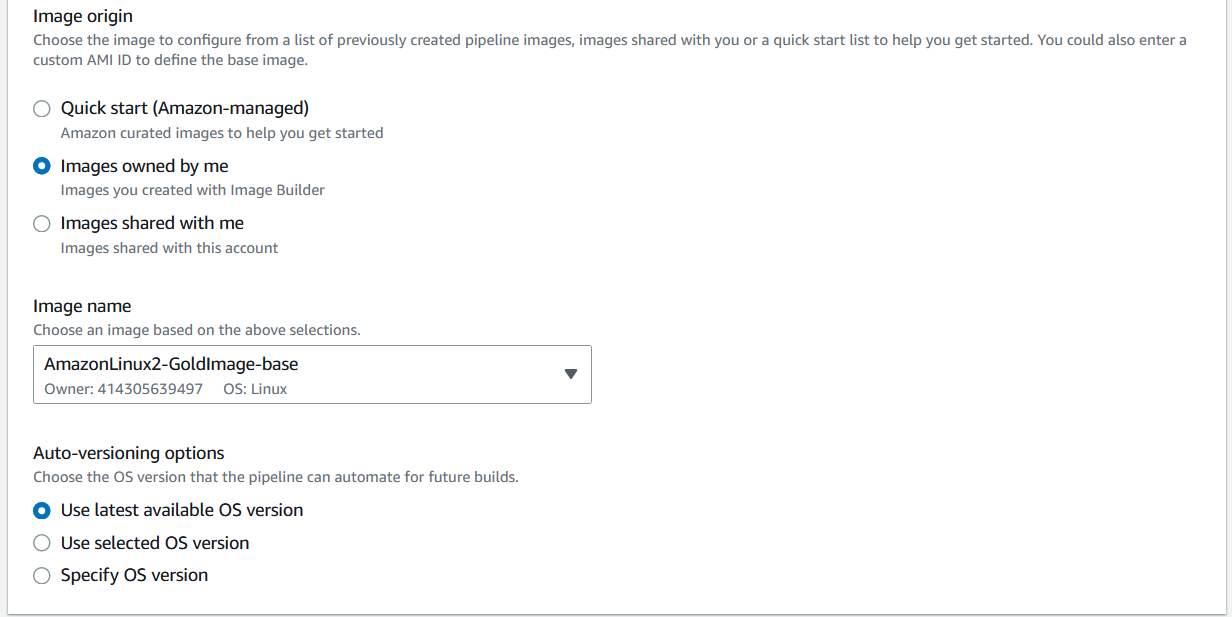
If you’re deploying an instance with the Lightsail console, launch scripts can be added to an instance at deployment. They are added in the ‘deploy instance’ page:

Image of Amazon Lightsail deploy an instance page

The launch script must be added before the instance is deployed, because launch scripts can’t retroactively run after deployment.

Anatomy of a Windows Launch Script

When deploying a Lightsail Windows instance, you can use a batch script or a PowerShell script in the ‘launch script’ textbox.  Of the two options, PowerShell is more extensible and provides greater flexibility for configuration and control.

If you choose to write your launch script as a batch file, you must add <script> </script> tags at the beginning and end of your code respectively. Alternatively, a launch script in PowerShell, must use the <powershell></powershell> tags in a similar fashion.

After the closing </script> or </powershell> tag, you must add a <persist></persist> tag on the following line. The persist tag is used to determine if this is a run-once command or if it should run every time your instance is rebooted or changed from the ‘Stop’ to ‘Start’ state. If you want your script to run every time the instance is rebooted or started, then you must set the persist tag to ‘true’. If you want your launch script to just run once, then you would set your persist tag to ‘false’.

Anatomy of a Linux Launch Script

Like a Windows launch script, a Linux launch script requires specific code on the first row of the textbox to successfully execute during deployment. You must place ‘#!/bin/bash’ as the first line of code to set the shell that executes the rest of the script. After first line of code, you can continue adding additional commands to achieve the results you want.

How do I know if my Launch Script ran successfully?

Although running launch scripts is convenient to create a baseline instance, it’s possible that your instance doesn’t achieve the desired end-state because of an error in your script or permissions issues. You must troubleshoot to see why the launch script didn’t complete successfully. To find if the launch script ran successfully, refer to the instance logs to determine whether your launch script was successful or not.

For Windows, the launch log can be found in: C:\ProgramData\Amazon\EC2-Windows\launch\Log\UserdataExecution.log. Note that ProgramData is a hidden folder, and unless you access the file from PowerShell or Command Prompt, you must use Windows File Explorer (`View > Show > Hidden items`) folders to see it.

For Linux, the launch log can be found in: /var/log/cloud-init-output.log and can be monitored after your instance launches by tailing the log by typing the following in the terminal:

tail -f /var/log/cloud-init-output.log

If you want to see the entire log file including commands that have already run before you opened the log file, then you can type the following in the terminal:

less +F /var/log/cloud-init-output.log

On a Windows instance, an easy way to monitor the UserdataExecution.log is to add the following code in your launch script, which creates a shortcut to tail or watch the log as commands are executing:

# Create a log-monitoring script to monitor the progress of the launch script execution

$monitorlogs = @"
get-content C:\ProgramData\Amazon\EC2-Windows\launch\Log\UserdataExecution.log -wait
"@

# Save the log-monitoring script to the desktop for the user

$monitorlogs | out-file -FilePath C:\Users\Administrator\Desktop\MonitorLogs.ps1 -Encoding utf8 -Force

</powershell>
<persist>false</persist>

If the script was executed, then the last line of the log should say ‘{Timestamp}: User data script completed’.

However, if you want more detail, you can build the logging into your launch script. For example, you can append a text or log file with each command so that you can read the output in an easy-to-access location:

<powershell>
# Set the location for the log file. In this case,
# it will appear on the desktop of your Lightsail instance
$loc = "c:\Users\Administrator\Desktop\mylog.txt"

# Write text to the log file
Write-Output "Starting Script" >> $loc

# Download and install Chocolatey to do unattended installations of the rest of the apps.
iex ((New-Object System.Net.WebClient).DownloadString('https://chocolatey.org/install.ps1'))

# You could run commands like this to output the progress to the log file:

# Install vscode and all dependencies
choco install -y vscode --force --force-dependencies --verbose >> $loc

# Install git and all dependencies
choco install -y git --force --force-dependencies --verbose >> $loc

# Completed
Write-Output "Completed" >> $loc
</powershell>
<persist>false</persist>

This code creates a log file, outputs data, and appends it along the way. If there is an issue, then you can see where the logs stopped or errors appeared.

For Ubuntu and Amazon Linux 2

If the cloud-init-output.log isn’t comprehensive enough, then you can re-direct the output from your commands to a log file of your choice. In this example, we create a log file in the /tmp/ directory and push all output from our commands to this file.

# Create the log file
touch /tmp/launchscript.log

# Add text to the log file if you so choose
echo 'Starting' >> /tmp/launchscript.log

# Update package index
sudo apt update >> /tmp/launchscript.log

# Install software to manage independent software vendor sources
sudo apt -y install software-properties-common >> /tmp/launchscript.log

# Add the repository for all PHP versions
sudo add-apt-repository -y ppa:ondrej/php >> /tmp/launchscript.log

# Install Web server, mySQL client, PHP (and packages), unzip, and curl
sudo apt -y install apache2 mysql-client-core-8.0 php8.0 libapache2-mod-php8.0 php8.0-common php8.0-imap php8.0-mbstring php8.0-xmlrpc php8.0-soap php8.0-gd php8.0-xml php8.0-intl php8.0-mysql php8.0-cli php8.0-bcmath php8.0-ldap php8.0-zip php8.0-curl unzip curl >> /tmp/launchscript.log

# Any final text you want to include
echo 'Completed' >> /tmp/launchscript.log

It’s possible to check the logs before the launch script has finished executing. One way to follow along is to ‘tail’ the log file. This lets you stream all updates as they occur. You can monitor the log using:

‘tail -f /tmp/launchscript.log’. </code>

Using Launch Scripts from AWS Command Line Interface (AWS CLI)

You can deploy their Lightsail instances from the AWS Command Line Interface (AWS CLI) instead of the Lightsail console. You can add launch scripts to the AWS CLI command as a parameter by creating a variable with the script and referencing the variable, or by saving the launch script as a file and referencing the local file location on your computer.

The launch script is still written the same way as the previous examples. For a Windows instance with a PowerShell launch script, you can deploy a Lightsail instance with a launch script with the following code:

# PowerShell script saved in the Downloads folder:

$loc = "c:\Users\Administrator\Desktop\mylog.txt"

# Write text to the log file

Write-Output "Starting Script" >> $loc

# Download and install Chocolatey to do unattended installations of the rest of the apps.

iex ((New-Object System.Net.WebClient).DownloadString('https://chocolatey.org/install.ps1'))

# You could run commands like this to output the progress to the log file:

# Install vscode and all dependencies

choco install -y vscode --force --force-dependencies --verbose >> $loc

# Install git and all dependencies

choco install -y git --force --force-dependencies --verbose >> $loc

# Completed

Write-Output "Completed" >> $loc

AWS CLI code to deploy a Windows Server 2019 medium instance in the us-west-2a Availability Zone:

aws lightsail create-instances \

--instance-names "my-windows-instance-1" \

--availability-zone us-west-2a \

--blueprint-id windows_server_2019 \

--bundle-id medium_win_2_0 \

--region us-west-2 \

--user-data file://~/Downloads/powershell_script.ps1

Clean up

Remember to delete resources when you are finished using them to avoid incurring future costs.

Conclusion

You now have the understanding and examples of how to create and troubleshoot Lightsail launch scripts both through the Lightsail console and AWS CLI. As demonstrated in this blog, using launch scripts, you can increase your productivity and decrease the deployment time and configuration of your applications. For more examples of using launch scripts, check out the aws-samples GitHub repository. You now have all the foundational building blocks you need to successfully script automated instance configuration. To learn more about Lightsail, visit the Lightsail service page.

Building a high-performance Windows workstation on AWS for graphics intensive applications

Post Syndicated from Macey Neff original https://aws.amazon.com/blogs/compute/building-a-high-performance-windows-workstation-on-aws-for-graphics-intensive-applications/

This blog post is written by Mike Lim, Senior Public Sector SA.

Video editing, professional visualization, and video games can be resource demanding applications that require high performance Windows workstations with GPUs. When developing these resource demanding applications, a high-performance remote display protocol is desirable in order to access the instances’ graphical desktops from the internet. Using NICE DCV provides a bandwidth-adaptive streaming protocol that provides near real-time responsiveness without compromising image quality. Customers using NICE DCV can leverage Amazon EC2 G4 and Amazon EC2 G5 GPU instances which support graphic-intensive applications in the cloud using a pay-as-you-go pricing model. By using Amazon Elastic Compute Cloud (Amazon EC2) with NICE DCV, customers can run graphically intensive applications remotely and stream their user interface to simpler client machines, eliminating the need for expensive dedicated workstations.

This post shows how you can provision and manage an Amazon EC2 GPU Windows instance and access it via the high-performance NICE DCV remote display protocol.

Solution overview

The solution is illustrated in the following figure.

Solution overview

Figure 1: Solution overview

We used the AWS CloudFormation Infrastructure-as-Code (IaC) service to provision our solution. Our CloudFormation template provides the following functionality:

1.       Using AWS CloudFormation, you can specify your choice of EC2 instance type, the Amazon Virtual Private Cloud (Amazon VPC), and subnet in which to provision. You also have the option to assign a static IPv4 address. NICE DCV server is installed to provide remote access, and you can specify the choice of graphics driver to install.

2.       A security group is created and associated with the EC2 instance, and it acts as a firewall.

3.       An AWS Identity and Access Management (IAM) role is created and associated with the EC2 instance using an instance profile. It lets your instance access Amazon Simple Storage Service (Amazon S3) buckets for NICE DCV server license validation, and download and install the latest graphics drivers.

4.       The IAM role also makes sure that your EC2 instance can be managed by AWS Systems Manager. This service provides in-browser command line and graphical access to your Windows instance via Session Manager and Fleet Manager from the AWS Management Console.

Walkthrough

The following sections walk through the steps to setup and maintain your graphics workstation. To begin, you need an AWS account. For this walkthrough, we provision a g5.xlarge instance for cloud gaming.

Check instance type availability

For best performance and lowest latency, you will want to provision EC2 in the AWS Region nearest to you. Before proceeding, verify that the g5.xlarge instance type is available in your desired AWS Region, and the Availability Zones (AZs) in which it is available.

Log in to your Amazon EC2 console and select your AWS Region. From the navigation pane, choose Instance Types to view the instance types available. In the search bar, filter instances types to the specific instance type you want, in this case g5.xlarge. Toggle the display preferences (gear) icon to display Availability zones column.

In the following screenshot, the g5.xlarge instance is available in two of the three AZs in eu-west-2 Europe London Region.

Amazon EC2 console instance types

Figure 2: Amazon EC2 console instance types

Check Amazon EC2 running on-demand G instances quota

Your AWS account has a limit on the number and type of EC2 instances types you can run, and you need to make sure you have enough quota to run the g5.xlarge instance.

Go to the Service Quotas console for your AWS Region. Under AWS services in the navigation pane, select Amazon Elastic Compute Cloud (Amazon EC2) and search for Running On-Demand G and VT instances. Verify that the Applied quota value number is equal or more than the number of vCPUs for the instance size you need. In the following screenshot, the applied quota value is 64. It lets us launch instance sizes from 4 vCPUs xlarge up to 64 vCPUs 16xlarge instance size.

Service Quotas console

Figure 3: Service Quotas console

You can request a higher quota value by selecting Request quota increase.

Using CloudFormation template

Download the CloudFormation template file from aws-samples GitHub repository. Go to the CloudFormation console for your AWS Region to create a stack, and upload your downloaded file.

The CloudFormation parameters page is divided into the following sections:

  1. AMI and instance type
  2. EC2 configuration
  3. Allowed inbound source IP prefixes to NICE DCV port 8443
  4. EBS volume configuration

We go through the configuration settings for each section in detail.

AMI and instance type

In this section, we select the Windows Amazon Machine Image (AMI) to use, EC2 instance type to provision, and graphics driver to install. The default AMI is Microsoft Windows Server 2022.

Replace the instanceType value with g5.xlarge.

CloudFormation parameters: AMI and instance type

Figure 4: CloudFormation parameters: AMI and instance type

Select driverType based on your instance type and the following use case:

  1. AMD: select this for instance types with AMD GPU (G4ad instance).
  2. NVIDIA-Gaming: select this to install the NVIDIA gaming driver, which is optimized for gaming (G5 and G4dn instances).
  3. NVIDIA-GRID: select this to install the GRID driver, which is optimized for professional visualization applications that render content such as 3D models or high-resolution videos (G5, G4dn, and G3 instances).
  4. none: select this option for accelerated computing instances, such as P2 and P3 instances where you download and install public NVIDIA drivers manually.
  5. NICE-DCV: this installs the NICE DCV Virtual Display driver and is suitable for all other instance types.

Note that GRID and NVIDIA gaming drivers’ downloads are available to AWS customers only. Upon installation of the software, you are bound by the terms of the NVIDIA GRID Cloud End User License Agreement.

For our walkthrough, select NVIDIA-Gaming for driverType.

Amazon EC2 configuration

In this section, we specify the VPC and subnet in which to provision our EC2 instance. You can select default VPC from the vpcID dropdown. Make sure that the subnetID value you select is in your selected VPC and resides in an AZ that has your instance type offering. You can also change the EC2 instance name.

Select Yes for the assignStaticIP option if you want to associate a static Internet IPv4 address. Note that there is a small hourly charge when the instance is not running.

CloudFormation parameters: Amazon EC2 configuration

Figure 5: CloudFormation parameters: Amazon EC2 configuration

Allowed inbound source IP prefixes to NICE DCV port 8443

Here, we specify the source prefixes allowed to access our instance. The default values allow access from all addresses. To secure access to your instance, you may want to limit the source prefix to your IP address.

To get your IPv4 address, go to https://checkip.amazonaws.com and append /32 to the value for ingressIPv4. The default VPC and subnet is IPv4 only. Therefore, you can enter ::1/128 to explicitly block all IPv6 access for ingressIPv6.

CloudFormation parameters: Allowed inbound source IP prefixes

Figure 6: CloudFormation parameters: Allowed inbound source IP prefixes

Amazon EBS volume configuration

The default Amazon Elastic Block Store (Amazon EBS) volume size is 30 GiB. You can specify a larger size by changing the volumeSize value.

CloudFormation parameters: Amazon EBS volume configuration

Figure 7: CloudFormation parameters: Amazon EBS volume configuration

Continue to provision your stack.

NICE DCV client

NICE DCV provides an HTML5 client for web browser access. For performance and additional features, such as QUIC UDP transport protocol support and USB remotization support, install the native client from the NICE DCV download page. NICE DCV offers native clients for Windows, MacOS for both Intel and Apple M1 processors, and modern Linux distributions including RHEL, SUSE Linux, and Ubuntu.

Cloudformation Outputs

Once provisioning is complete, go to the Outputs section.

CloudFormation Outputs

Figure 8: CloudFormation Outputs

The following URLs are available.

  1. DCVwebConsole
  2. EC2instance
  3. RdpConnect
  4. SSMsessionManager

We go through the purpose of each URL in the following sections.

SSMsessionManager: Change administrator password

To log in, you must specify an administrator password. Open the SSMsessionManager value URL in a new browser tab and run the command net user administrator <YOUR-PASSWORD> where <YOUR-PASSWORD> is the password on which you decided.

Systems Manager session manager

Figure 9: Systems Manager session manager

DCVwebConsole: Connecting to the EC2 instance

Copy DCVWebConsole value, open the NICE DCV client from your local machine and either use the copied value or the IP address to connect. Log in as administrator with the password that you have configured. Alternatively, enter the URL in the format dcv://<EC2-IP-Address> in a browser URL bar to automatically launch and connect a locally installed NICE DCV client to your EC2 instance.

NICE DCV client

Figure 10: NICE DCV client

EC2instance: manage EC2 instance

Use this link to manage your EC2 instance in the Amazon EC2 console. If you did not select the static IP address option, then use this page to get the assigned IP address whenever you stop and start your instance.

RdpConnect: Fleet Manager console access

The RdpConnect link provides in-browser Remote Desktop Protocol (RDP) console access to your Windows instance. Choose User credentials for Authentication Type. Enter administrator for username and the password that you have configured.

Fleet Manager Remote Desktop

Figure 11: Fleet Manager Remote Desktop

Updating NICE DCV server

To update NICE DCV server, log in via Fleet Manager Remote Desktop and run c:\users\administrator\update-DCV.cmd script. In the following screenshot, we successfully upgraded NICE DCV server from version 2022.2-14521 to 2023.0-15065.

Updating NICE DCV server

Figure 12: Updating NICE DCV server

Updating graphics drivers

You can use the download-<DRIVER_TYPE>-driver.cmd batch file to download the latest graphics driver for your instance type GPU. Downloaded files are located in the Downloads\Drivers folder.

Graphics driver download scripts

Figure 13: Graphics driver download scripts

AWS Command Line interface (AWS CLI v2) is installed in the instance. You can use it to view the different versions available on the driver S3 bucket. For example, the command aws s3 ls –recursive s3://nvidia-gaming/windows/ | sort /R lists NVIDIA gaming drivers available for download. NVIDIA GRID and AMD drivers are in the s3://ec2-windows-nvidia-drivers and s3://ec2-amd-windows-drivers S3 buckets respectively.

Listing graphics drivers on S3 bucket

Figure 14: Listing graphics drivers on S3 bucket

Use the command aws s3 cp s3://<S3_BUCKET_PATH>/<FILE-NAME>. to copy a specific driver from the S3 bucket to your local directory.

You can refer to Install NVIDIA drivers on Windows instances and Install AMD drivers on Windows instances for NVIDIA and AMD drivers installation instructions respectively.

Customizing your EC2 instance environment

You may want to customize the instance to your needs. For NVIDIA GPU instances, you can optimize GPU settings to achieve the best performance.

If you are doing video editing, then you can enable high color accuracy, configure multi-channel audio, and enable accurate audio/video sync. For gaming, you may enable gamepad support to use a DualShock 4 or Xbox 360 controller. NICE DCV session storage is enabled. This lets you transfer files using NICE DCV client. More configuration options are available from the NICE DCV User Guide and Administrator Guide.

Terminating your EC2 instance

When you have finished using your EC2 instance, you can release all provisioned resources by going to CloudFormation console to delete your stack.

Conclusion

The Amazon G4 and G5 GPU instance types are suitable for graphics-intensive applications, and NICE DCV provides a responsive and high image quality display protocol for remote access. Using the CloudFormation template from amazon-ec2-nice-dcv-samples GitHub site, you can build and maintain your own high performance Windows graphics workstation in the AWS cloud

New Amazon EC2 Instances (C7gd, M7gd, and R7gd) Powered by AWS Graviton3 Processor with Local NVMe-based SSD Storage

Post Syndicated from Channy Yun original https://aws.amazon.com/blogs/aws/new-amazon-ec2-instances-c7gd-m7gd-and-r7gd-powered-by-aws-graviton3-processor-with-local-nvme-based-ssd-storage/

We launched Amazon EC2 C7g instances in May 2022 and M7g and R7g instances in February 2023. Powered by the latest AWS Graviton3 processors, the new instances deliver up to 25 percent higher performance, up to two times higher floating-point performance, and up to 2 times faster cryptographic workload performance compared to AWS Graviton2 processors.

Graviton3 processors deliver up to 3 times better performance compared to AWS Graviton2 processors for machine learning (ML) workloads, including support for bfloat16. They also support DDR5 memory that provides 50 percent more memory bandwidth compared to DDR4. Graviton3 also uses up to 60 percent less energy for the same performance as comparable EC2 instances, which helps you reduce your carbon footprint.

The C7g instances are well suited for compute-intensive workloads, such as high performance computing (HPC), batch processing, ad serving, video encoding, gaming, scientific modeling, distributed analytics, and CPU-based machine learning inference. The M7g instances are for general purpose workloads such as application servers, microservices, gaming servers, mid-sized data stores, and caching fleets. The R7g instances are a great fit for memory-intensive workloads such as open-source databases, in-memory caches, and real-time big data analytics.

Today, we’re adding a d variant to all three instance families. The new Amazon EC2 C7gd, M7gd, and R7gd instance types have NVM Express (NVMe) locally attached up to 2 x 1.9 TB SSD drives that are physically connected to the host server and provide block-level storage that is coupled to the lifetime of the instance. These instances have up to 45 percent better real-time NVMe storage performance than comparable Graviton2-based instances.

These are a great fit for applications that need access to high-speed, low-latency local storage, including those that need temporary storage of data for scratch space, temporary files, and caches. The data on an instance store volume persists only during the life of the associated EC2 instance.

Here are the specs for these instances:

Instance Size vCPU Memory
(GiB)
Local NVMe Storage (GB) Network Bandwidth
(Gbps)
EBS Bandwidth
(Gbps)
C7gd/M7gd/R7gd C7gd/M7gd/R7gd C7gd/M7gd/R7gd
medium 1 2/ 4 / 8 1 x 59 Up to 12.5 Up to 10
large 2 4 / 8 / 16 1 x 118 Up to 12.5 Up to 10
xlarge 4 8 / 16 / 32 1 x 237 Up to 12.5 Up to 10
2xlarge 8 16 / 32 / 64 1 x 474 Up to 15 Up to 10
4xlarge 16 32 / 64 / 128 1 x 950 Up to 15 Up to 10
8xlarge 32 64 / 128 / 256 1 x 1900 15 10
12xlarge 48 96 / 192/ 384 2 x 1425 22.5 15
16xlarge 64 128 / 256 / 512 2 x 1900 30 20

These instances are built on the AWS Nitro System, a combination of AWS-designed dedicated hardware and a lightweight hypervisor that allows the delivery of isolated multitenancy, private networking, and fast local storage. They provide up to 20 Gbps Amazon Elastic Block Store (Amazon EBS) bandwidth and up to 30 Gbps network bandwidth. The 16xlarge instances also support Elastic Fabric Adapter (EFA) for applications that need a high level of inter-node communication.

Now Available
Amazon EC2 C7gd, M7gd, and R7gd instances are now available in the following AWS Regions: US East (Ohio), US East (N. Virginia), US West (Oregon), and Europe (Ireland). As usual with Amazon EC2, you only pay for what you use. For more information, see the Amazon EC2 pricing page.

If you’re optimizing applications for Arm architecture, be sure to have a look at our Getting Started collection of resources or learn more about AWS Graviton3-based EC2 instances.

To learn more, visit our Amazon EC2 C7g instances, M7g instances or R7g instances page, and please send feedback to AWS re:Post for EC2 or through your usual AWS Support contacts.

Channy

New – Amazon EC2 Hpc7g Instances Powered by AWS Graviton3E Processors Optimized for High Performance Computing Workloads

Post Syndicated from Channy Yun original https://aws.amazon.com/blogs/aws/new-amazon-ec2-hpc7g-instances-powered-by-aws-graviton3e-processors-optimized-for-high-performance-computing-workloads/

At AWS re:Invent 2022, Adam Selipsky, CEO of AWS, explained high performance computing (HPC) workloads typically can either be compute-intensive, compute- and networking-intensive, or data- and memory-intensive in his keynote.

Compute workloads include weather forecasting, computational fluid dynamics, and financial options pricing. To help with this, you have Amazon EC2 Hpc6a instances, which deliver up to 65 percent better price performance over comparable compute optimized x86-based instances.

Other HPC workloads require modeling the performance of complex structures—things like wind turbines, concrete buildings, and industrial equipment. Without enough data and memory, these models can take days or weeks to run in a cost-effective way. The Amazon EC2 Hpc6id instance is designed to deliver leading price performance for data and memory-intensive HPC workloads with higher memory bandwidth per core, faster local solid-state drive (SSD) storage, and enhanced networking with Elastic Fabric Adapter (EFA).

Announcing Amazon EC2 Hpc7g Instances
Compute-intensive HPC workloads such as weather forecasting, computational fluid dynamics, and financial options pricing also require more network performance, even better price performance, and greater energy efficiency.

Today we are announcing the general availability of Amazon EC2 Hpc7g instances, a new purpose-built instance type for tightly coupled compute and network-intensive HPC workloads.

Hpc7g instances are powered by AWS Graviton3E processors that provide up to two times better floating-point performance and 200 Gbps dedicated EFA bandwidth than EC2 C6gn instances powered by AWS Graviton2 processors and are up to 60 percent more energy efficient than comparable x86 instances.

Here’s a quick infographic that shows you how the Hpc7g instances and the Graviton3E processors compare to previous instances and processors:

Hpc7g instances feature sizes of up to 64 cores of the latest AWS custom Graviton3E CPUs with 128 GiB RAM. Here are the detailed specs:

Instance Name
CPUs RAM (GiB)
EFA Network Bandwidth (Gbps) Attached Storage
hpc7g.4xlarge 16 128 Up to 200 EBS Only
hpc7g.8xlarge 32 128 Up to 200 EBS Only
hpc7g.16xlarge 64 128 Up to 200 EBS Only

Hpc7g instances are the most cost-efficient option to scale your HPC clusters on AWS. If you are considering migrating your largest HPC workloads requiring tens of thousands of cores at scale to AWS, you can take advantage of up to 200 Gbps EFA bandwidth to reduce the latency and run message passing interface (MPI) applications on parallel computing architectures while ensuring minimized power consumption on Hpc7g instances.

You can choose to use smaller sizes of Hpc7g instances to pick a lower number of cores and evenly distribute memory and network resources across the remaining cores to increase per-core performance to help reduce software licensing costs.

You can also use Hpc7g instances with AWS ParallelCluster to offer a complete HPC run-time environment that spans both x86 and arm64 instance types, giving you the flexibility to run different workload types within the same HPC cluster. You can compare and contrast performance, thus making it easier to find out what’s best for you and enabling easier porting of your workload.

Customer Story
The Water Institute is an independent, non-profit applied research organization that works across disciplines to advance science and develop integrated methods used to solve complex environmental and societal challenges.

They benchmarked the Hpc7g instances with 200 Gbps EFA using the Advanced Circulation (ADCIRC) model. ADCIRC is deployed throughout many US government agencies to simulate the movement of water due to astronomic tides, riverine flows, and atmospheric forces, including hurricanes and it is often used for real-time forecasting applications and design studies.

The model run for this application is targeted at Southern Louisiana and is the basis for most of the analysis conducted there including levee design, planning studies, and real-time hurricane storm surge forecasting applications. The left graphic above shows the full extent of the domain, while to the right of that, the high-resolution area targeted at Southern Louisiana shows flooding around the levees in New Orleans during a simulation of Hurricane Katrina.

The model contains 1.6 million vertices and 3 million elements. It’s these parameters that affect the computational complexity of the simulations. The simulations depict 18 days of astronomic tide, river inflows, and atmospheric wind and pressure forcing.

The Water Institute benchmarked against many of the instance types that would be useful for their workload types at AWS, including c6gn.16xlarge, hpc7g.16xlarge, hpc6a.48xlarge, and hpc6id.36xlarge.

The Hpc7g instance shows more than 40 percent better performance than the C6gn instance and has comparable performance to other high performance x86 instance types but with a better price-to-performance ratio. With Hpc7g instances, the Water Institute can lower its costs while maintaining the performance levels they expect.

RIKEN, who has built the powerful supercomputer, FUGAKU using arm64, is collaborating with AWS to create a virtual Fugaku using Hpc7g with Graviton3E to support Japanese manufacturers’ increasing demand for compute power. RIKEN has already confirmed that multiple Fugaku applications provide excellent performance on the AWS Graviton3E processor in the AWS cloud environment.

Also, Siemens has optimized the scalability of Simcenter STAR-CCM+ across a broad range of CPU and GPU instances on AWS. This technology is supported on Linux and available through Arm-based EC2 instances or the Fugaku supercomputer.

To hear more voices of customers and partners such as Ansys, Arup, CERFACS, ESI, Jij, ParTec, Rescale, and TotalCAE, see the Hpc7g instances page.

Now Available
Amazon EC2 Hpc7g instances are now generally available in the US East (N. Virginia) Region for purchase in On-Demand, Reserved Instance, and Savings Plan form.

To learn more, see the Amazon EC2 Hpc7g instances page. Give it a try, and please send feedback to AWS re:Post for High Performance Compute or through your usual AWS support contacts.

Channy

Deploying an automated Amazon CloudWatch dashboard for AWS Outposts using AWS CDK

Post Syndicated from Sheila Busser original https://aws.amazon.com/blogs/compute/deploying-an-automated-amazon-cloudwatch-dashboard-for-aws-outposts-using-aws-cdk/

This post is written by Enrico Liguori, Networking Solutions Architect, Hybrid Cloud and Sumeeth Siriyur, Sr. Hybrid Cloud Solutions Architect.

AWS Outposts is a fully managed service that brings the same AWS infrastructure, services, APIs, and tools to virtually any data center, colocation space, manufacturing floor, or on-premises facility where it might be needed. With Outposts, you can run some AWS services on-premises and connect to a broad range of services available in the local AWS Region. Outposts supports workloads requiring low latency, local data processing, data residency, and application migration.

Outposts capacity is driven as per your compute and storage requirements to run workloads. You can monitor Outposts resources using metrics gathered by Amazon CloudWatch. Using these metrics, you can effectively monitor and manage the Outposts resources as they would in the Region, levereging cloud native tools such as CloudWatch dashboards. Check the Monitoring best practices for AWS Outposts blog post to dive deep into the available monitoring options for Outposts.

CloudWatch dashboards are customizable home pages in the CloudWatch console that can be used to monitor resources running on Outposts in a single view. For example, you can monitor in a single pane the number Amazon EC2 instances used per EC2 instance type, the available capacity of Amazon EBS volumes and Amazon S3 buckets, and the operational status of the service link of Outposts.

As a you start deploying additional Outposts resources as a part of their capacity expansion, they must all be integrated and visualized within CloudWatch in an automated way. Traditionally CloudWatch dashboards are built manually and may be time consuming to tune. This post provides also an overview of building CloudWatch dashboards in an automated way using AWS Cloud Development Kit (AWS CDK).

Overview

CloudWatch metrics available to monitor Outposts resources and capacity

CloudWatch metrics for Outposts are available to customers in all public AWS Regions and AWS GovCloud (US) at no additional cost. We can classify the available metrics in two main categories:

To identify the metrics published under the service specific namespaces, we can leverage metadata in the form of tags. A tag is a label that you assign to an AWS resource and consists of a key and an optional value. For the purpose of the monitoring strategy described in this post, we use a tag that contains the OutpostID of the Outpost where the resource is deployed. In this way, we can easily filter the CloudWatch metrics that we would like to show in our dashboard.

To enforce the assignment of tags to our resources we can implement a tagging strategy using AWS tag Policies and Service Control Policies (SCPs).

The following sections describe two different methods to build a CloudWatch dashboard that includes the different types of metrics described so far. In both cases, we see how particularly useful the presence of tags is to identify the service-specific metrics.

Manual approach to building a CloudWatch dashboard for Outposts

This section describes a manual (i.e., non-automated) approach to building a dashboard that could summarize both the capacity utilization metrics and the service specific metrics for your resources running on Outposts.

The benefit of this approach is that we can implement a fully operational dashboard directly from the CloudWatch console. However, it will simultaneously require more effort to properly tune the dashboard to satisfy your monitoring requirements.

You can start creating the dashboard opening the CloudWatch console and following the steps listed in the public documentation.

To display a metric under AWS/Outposts namespace we can choose any of the widgets available. Based on the nature of the data, we can choose different types of Widgets such as Number, Line, Gauge, Explorer, or you can even build your own custom widget.

Together with the Widget type, we must select Outposts namespace in the metric graph dialog box and then navigate to the specific metric of interest.

In case we are creating the dashboard in a different account than the Outposts owner, we must select the right account in the View data drop-down menu to see the Outposts metric in which we are interested.

View data drop-down menu

After selecting one or more metrics we can select Create widget button.

For the service specific metrics, we recommend using the explorer widget. In this way, we can utilize the tagging strategy described earlier to automatically identify the metrics belonging to the resources running on Outposts. Check the documentation page for a step-by-step guide for creating an explorer widget based on tags.

Automated outpost dashboard

After we’ve seen how to build a dashboard manually from the console, in this secton we describe an automated approach to deploy a dashboard for Outposts through AWS CDK.

AWS CDK is an open source software development framework to model and provision your cloud application resources using familiar programming languages, including TypeScript, JavaScript, Python, C#, and Java. For the solution in this post, we use Python.

Architecture overview

The AWS CDK stack described in this post, assumes that the resources running on Outposts (EC2 instances, S3 buckets, Application Load Balancers (ALBs), and RDS instances) are tagged using the tagging strategy described earlier.

Specifying a tag name and a tag value in a configuration file automatically discovers the resources with that tag and adds the related metrics to the CloudWatch dashboard.

Together with the service specific metrics, it creates a series of widgets that we can use to monitor the capacity available and utilized in each Outpost that belongs to the account where the script is running.

The workflow is made of the following phases:

  1. The AWS CDK stack creates an AWS CodeCommit repository and uploads its own code into it. The code contains a series of modules, one for each section of the CloudWatch dashboard. A section of the dashboard contains one or more widgets showing the metrics of a specific service.
  2. To maintain the CloudWatch dashboard always up-to-date with the resources matching the tag, it creates a pipeline in AWS CodePipeline that can dynamically create and or update the dashboard. The pipeline runs the code in the CodeCommit repository and is made of two stages. In the first one, the build stage, it builds the dependencies needed by the AWS CDK stack. In the second stage, the Deploy stage, it loads and runs the modules used to build the dashboard.
  3. Each module contains the code to automatically discover the tagged resources of a specific service. This discovery phase uses standard AWS APIs called through the Python SDK Boto3.
  4. Based on the results of the discovery phase, AWS CDK produces an AWS CloudFormation template containing the definition of the CloudWatch dashboard sections. The template is submitted to CloudFormation.
  5. CloudFormation creates or, if already defined, updates the CloudWatch dashboard.
  6. Together with the dashboard, the AWS CDK script also contains the definition of a CloudWatch Event that, once deployed, triggers the pipeline each time a resource tagged with the specified tag is created or destroyed.

Prerequisites

To implement the solution presented in this post, you must configure:

  1. git as distributed version control system.
  2. In case it is the first time that you’re using AWS CDK in this account and region, you must:

a. Install the AWS CDK, and its prerequisites, following these instructions.

b. Go through the AWS CDK bootstrapping process. This is required only for the first time that we use AWS CDK in a specific AWS environment (an AWS environment is a combination of an AWS account and Region).

How to install

Step 1: Clone the AWS CDK code hosted on GitHub with:

$ git clone https://github.com/aws-samples/automated-cloudwatch-dashboard.git

Step 2: enter the directory using the following:

$ cd  automated-cloudwatch-dashboard/

Step 3: Install the needed Python dependencies with:

$ pip install -r requirements.txt

Step 4: Modify the configuration file

Before deploying the stack, we must modify the configuration file to specify the tag we use for identifying our resources running on Outposts. Open the file with the name config.yaml with your preferred text editor and specify:

      • A name for the dashboard. The default name used is Automated-CloudWatch-Dashboard.
      • Replace <tag_name> placeholder following the tag_name variable with the tag name used to tag the resources that you want to include in the dashboard.
      • Replace <tag_value> placeholder under tag_values variable with the tag value that you used.

Here is an example config.yaml configuration file:

dashboard_name: Automated-CloudWatch-Dahsboard
tag_name: OutpostID
tag_values:
  - op-1234567890abcdefg 

Stack deployment

We can deploy the stack with the following:

$ cdk deploy

At the end of the deployment process, the pipeline that creates the dashboard is provisioned. You can now go to your CloudWatch console to view it.

Automated Outposts dashboard overview

Now that we have built our dashboard, let’s review each section:

  1. Outpost capacity

Outpost Capacity diagram

The AWS CDK stacks define a capacity section for each Outpost available to the AWS account where the script runs.

In this section, we find four widgets showing metrics published under the AWS/Outpost namespace. The first widget shows for each EC2 instance type available on the Outposts the number of instances utilized and available for that instance type. In the second row, we can visualize the available capacity for the Amazon EBS volumes and for the S3 buckets. The last widget shows the operational status of the service link of Outposts.

2. EC2 instances

CPU, Network, and Disk Utilization for an EC2 instance diagram

In this section of the dashboard, we find the metrics showing the CPU, Network, and Disk Utilization for an EC2 instance. It has defined a section of this type for each EC2 instance with a tag assigned matching the name and the value specified in the configuration file of the script.

3. Application Load Balancer

The ALB section aggregates metrics showing the operational status of a load balancer hosted on Outposts

The ALB section aggregates metrics showing the operational status of a load balancer hosted on Outposts. A section of this type is defined for each ALB with an assigned tag matching the one specified in the configuration file.

4. S3 buckets

The S3 buckets section diagram

The S3 buckets section is defined only once and aggregates the utilization metrics for all S3 buckets with an assigned tag.

5. AutoScaling group

The AutoScaling group section diagram

The AutoScaling group section can be used to monitor the number of instances in service in a specific AS group with a tag assigned. This section is defined once and can aggregate the metrics for multiple AutoScaling groups.

Clean up

To terminate the resources that we created in this post, run the following:

$ cdk destroy

Then, go to the Cloudformation console and delete the stack with the name “Deploy-AutomatedCloudWatchDashboard”.

Conclusion

In conclusion, this post demonstrates a manual way of creating CloudWatch Metrics dashboard using the CloudWatch console and an automated way using AWS CDK. The automated approach is also scalable by automatically discovering any new resources added to the existing Outposts in the your environment without any changes to the code.

Secure Connectivity from Public to Private: Introducing EC2 Instance Connect Endpoint

Post Syndicated from Sheila Busser original https://aws.amazon.com/blogs/compute/secure-connectivity-from-public-to-private-introducing-ec2-instance-connect-endpoint-june-13-2023/

This blog post is written by Ariana Rahgozar, Solutions Architect, and Kenneth Kitts, Sr. Technical Account Manager, AWS.

Imagine trying to connect to an Amazon Elastic Compute Cloud (Amazon EC2) instance within your Amazon Virtual Private Cloud (Amazon VPC) over the Internet. Typically, you’d first have to connect to a bastion host with a public IP address that your administrator set up over an Internet Gateway (IGW) in your VPC, and then use port forwarding to reach your destination.

Today we launched Amazon EC2 Instance Connect (EIC) Endpoint, a new feature that allows you to connect securely to your instances and other VPC resources from the Internet. With EIC Endpoint, you no longer need an IGW in your VPC, a public IP address on your resource, a bastion host, or any agent to connect to your resources. EIC Endpoint combines identity-based and network-based access controls, providing the isolation, control, and logging needed to meet your organization’s security requirements. As a bonus, your organization administrator is also relieved of the operational overhead of maintaining and patching bastion hosts for connectivity. EIC Endpoint works with the AWS Management Console and AWS Command Line Interface (AWS CLI). Furthermore, it gives you the flexibility to continue using your favorite tools, such as PuTTY and OpenSSH.

In this post, we provide an overview of how the EIC Endpoint works and its security controls, guide you through your first EIC Endpoint creation, and demonstrate how to SSH to an instance from the Internet over the EIC Endpoint.

EIC Endpoint product overview

EIC Endpoint is an identity-aware TCP proxy. It has two modes: first, AWS CLI client is used to create a secure, WebSocket tunnel from your workstation to the endpoint with your AWS Identity and Access Management (IAM) credentials. Once you’ve established a tunnel, you point your preferred client at your loopback address (127.0.0.1 or localhost) and connect as usual. Second, when not using the AWS CLI, the Console gives you secure and seamless access to resources inside your VPC. Authentication and authorization is evaluated before traffic reaches the VPC. The following figure shows an illustration of a user connecting via an EIC Endpoint:

Figure 1 shows a user connecting to private EC2 instances within a VPC through an EIC Endpoint

Figure 1. User connecting to private EC2 instances through an EIC Endpoint

EIC Endpoints provide a high degree of flexibility. First, they don’t require your VPC to have direct Internet connectivity using an IGW or NAT Gateway. Second, no agent is needed on the resource you wish to connect to, allowing for easy remote administration of resources which may not support agents, like third-party appliances. Third, they preserve existing workflows, enabling you to continue using your preferred client software on your local workstation to connect and manage your resources. And finally, IAM and Security Groups can be used to control access, which we discuss in more detail in the next section.

Prior to the launch of EIC Endpoints, AWS offered two key services to help manage access from public address space into a VPC more carefully. First is EC2 Instance Connect, which provides a mechanism that uses IAM credentials to push ephemeral SSH keys to an instance, making long-lived keys unnecessary. However, until now EC2 Instance Connect required a public IP address on your instance when connecting over the Internet. With this launch, you can use EC2 Instance Connect with EIC Endpoints, combining the two capabilities to give you ephemeral-key-based SSH to your instances without exposure to the public Internet. As an alternative to EC2 Instance Connect and EIC Endpoint based connectivity, AWS also offers Systems Manager Session Manager (SSM), which provides agent-based connectivity to instances. SSM uses IAM for authentication and authorization, and is ideal for environments where an agent can be configured to run.

Given that EIC Endpoint enables access to private resources from public IP space, let’s review the security controls and capabilities in more detail before discussing creating your first EIC Endpoint.

Security capabilities and controls

Many AWS customers remotely managing resources inside their VPCs from the Internet still use either public IP addresses on the relevant resources, or at best a bastion host approach combined with long-lived SSH keys. Using public IPs can be locked down somewhat using IGW routes and/or security groups. However, in a dynamic environment those controls can be hard to manage. As a result, careful management of long-lived SSH keys remains the only layer of defense, which isn’t great since we all know that these controls sometimes fail, and so defense-in-depth is important. Although bastion hosts can help, they increase the operational overhead of managing, patching, and maintaining infrastructure significantly.

IAM authorization is required to create the EIC Endpoint and also to establish a connection via the endpoint’s secure tunneling technology. Along with identity-based access controls governing who, how, when, and how long users can connect, more traditional network access controls like security groups can also be used. Security groups associated with your VPC resources can be used to grant/deny access. Whether it’s IAM policies or security groups, the default behavior is to deny traffic unless it is explicitly allowed.

EIC Endpoint meets important security requirements in terms of separation of privileges for the control plane and data plane. An administrator with full EC2 IAM privileges can create and control EIC Endpoints (the control plane). However, they cannot use those endpoints without also having EC2 Instance Connect IAM privileges (the data plane). Conversely, DevOps engineers who may need to use EIC Endpoint to tunnel into VPC resources do not require control-plane privileges to do so. In all cases, IAM principals using an EIC Endpoint must be part of the same AWS account (either directly or by cross-account role assumption). Security administrators and auditors have a centralized view of endpoint activity as all API calls for configuring and connecting via the EIC Endpoint API are recorded in AWS CloudTrail. Records of data-plane connections include the IAM principal making the request, their source IP address, the requested destination IP address, and the destination port. See the following figure for an example CloudTrail entry.

Figure 2 shows a sample cloud trail entry for SSH data-plane connection for an IAMUser. Specific entry:  Figure 2. Partial CloudTrail entry for an SSH data-plane connection

EIC Endpoint supports the optional use of Client IP Preservation (a.k.a Source IP Preservation), which is an important security consideration for certain organizations. For example, suppose the resource you are connecting to has network access controls that are scoped to your specific public IP address, or your instance access logs must contain the client’s “true” IP address. Although you may choose to enable this feature when you create an endpoint, the default setting is off. When off, connections proxied through the endpoint use the endpoint’s private IP address in the network packets’ source IP field. This default behavior allows connections proxied through the endpoint to reach as far as your route tables permit. Remember, no matter how you configure this setting, CloudTrail records the client’s true IP address.

EIC Endpoints strengthen security by combining identity-based authentication and authorization with traditional network-perimeter controls and provides for fine-grained access control, logging, monitoring, and more defense in depth. Moreover, it does all this without requiring Internet-enabling infrastructure in your VPC, minimizing the possibility of unintended access to private VPC resources.

Getting started

Creating your EIC Endpoint

Only one endpoint is required per VPC. To create or modify an endpoint and connect to a resource, a user must have the required IAM permissions, and any security groups associated with your VPC resources must have a rule to allow connectivity. Refer to the following resources for more details on configuring security groups and sample IAM permissions.

The AWS CLI or Console can be used to create an EIC Endpoint, and we demonstrate the AWS CLI in the following. To create an EIC Endpoint using the Console, refer to the documentation.

Creating an EIC Endpoint with the AWS CLI

To create an EIC Endpoint with the AWS CLI, run the following command, replacing [SUBNET] with your subnet ID and [SG-ID] with your security group ID:

aws ec2 create-instance-connect-endpoint \
    --subnet-id [SUBNET] \
    --security-group-id [SG-ID]

After creating an EIC Endpoint using the AWS CLI or Console, and granting the user IAM permission to create a tunnel, a connection can be established. Now we discuss how to connect to Linux instances using SSH. However, note that you can also use the OpenTunnel API to connect to instances via RDP.

Connecting to your Linux Instance using SSH

With your EIC Endpoint set up in your VPC subnet, you can connect using SSH. Traditionally, access to an EC2 instance using SSH was controlled by key pairs and network access controls. With EIC Endpoint, an additional layer of control is enabled through IAM policy, leading to an enhanced security posture for remote access. We describe two methods to connect via SSH in the following.

One-click command

To further reduce the operational burden of creating and rotating SSH keys, you can use the new ec2-instance-connect ssh command from the AWS CLI. With this new command, we generate ephemeral keys for you to connect to your instance. Note that this command requires use of the OpenSSH client. To use this command and connect, you need IAM permissions as detailed here.

Once configured, you can connect using the new AWS CLI command, shown in the following figure:
Figure 3 shows the AWS CLI view if successfully connecting to your instance using the one-click command. When running the command, you are prompted to connect and can access your instance.

Figure 3. AWS CLI view upon successful SSH connection to your instance

To test connecting to your instance from the AWS CLI, you can run the following command where [INSTANCE] is the instance ID of your EC2 instance:

aws ec2-instance-connect ssh --instance-id [INSTANCE]

Note that you can still use long-lived SSH credentials to connect if you must maintain existing workflows, which we will show in the following. However, note that dynamic, frequently rotated credentials are generally safer.

Open-tunnel command

You can also connect using SSH with standard tooling or using the proxy command. To establish a private tunnel (TCP proxy) to the instance, you must run one AWS CLI command, which you can see in the following figure:

Figure 4 shows the AWS CLI view after running the aws ec2-instance-connect open-tunnel command and connecting to your instance.Figure 4. AWS CLI view after running new SSH open-tunnel command, creating a private tunnel to connect to our EC2 instance

You can run the following command to test connectivity, where [INSTANCE] is the instance ID of your EC2 instance and [SSH-KEY] is the location and name of your SSH key. For guidance on the use of SSH keys, refer to our documentation on Amazon EC2 key pairs and Linux instances.

ssh ec2-user@[INSTANCE] \
    -i [SSH-KEY] \
    -o ProxyCommand='aws ec2-instance-connect open-tunnel \
    --instance-id %h'

Once we have our EIC Endpoint configured, we can SSH into our EC2 instances without a public IP or IGW using the AWS CLI.

Conclusion

EIC Endpoint provides a secure solution to connect to your instances via SSH or RDP in private subnets without IGWs, public IPs, agents, and bastion hosts. By configuring an EIC Endpoint for your VPC, you can securely connect using your existing client tools or the Console/AWS CLI. To learn more, visit the EIC Endpoint documentation.

AWS Week in Review – Automate DLQ Redrive for SQS, Lambda Supports Ruby 3.2, and More – June 12, 2023

Post Syndicated from Marcia Villalba original https://aws.amazon.com/blogs/aws/aws-week-in-review-automate-dlq-redrive-for-sqs-lambda-supports-ruby-3-2-and-more-june-12-2023/

Today I’m boarding a plane for Madrid. I will attend the AWS Summit Madrid this Thursday, and I will take Serverlesspresso with me. Serverlesspresso is a demo that we take to events, in where you can learn how to build event-driven architectures with serverless. If you are visiting an AWS Summit, most probably you will find one of our booths.

Serverlesspresso at Madrid

Last Week’s Launches
Here are some launches that got my attention during the previous week.

Amazon SQS – Customers were very excited when we announced the DLQ redrive for Amazon SQS as that feature helped them to easily redirect the failed messages. This week we added support for AWS SDK and CLI for this feature, allowing you to redrive the messages on the DLQ automatically, making it even easier to use this feature. You can read Seb’s blog post about this new feature to learn how to get started.

AWS Lambda – AWS Lambda now supports Ruby 3.2. Ruby 3.2 has many new improvements, for example, passing anonymous arguments to functions or having endless methods. Check out this blog post that goes in depth into each of the new features.

Amazon Fraud DetectorAmazon Fraud Detector supports event orchestration with Amazon EventBridge. This is a very important feature because now you can act on the different events that Fraud Detector emits, for example, send notifications to different stakeholders.

AWS Glue – This week, AWS Glue made two important announcements. First, it announced the general availability of AWS Glue for Ray, a new data integration engine option for AWS Glue. Ray is a popular new open-source compute framework that helps developers to scale their Python workloads. In addition, AWS Glue announced AWS Glue Data Quality, a new capability that automatically measures and monitors data lake and data pipeline quality.

Amazon Elastic Container Registry (Amazon ECR)AWS Signer and Amazon ECR announced a new feature that allows you to sign and verify container images. You can use Signer to validate that only container images you have approved are deployed in your Amazon Elastic Kubernetes Service (Amazon EKS) clusters.

Amazon QuickSightAmazon QuickSight now supports APIs to automate asset deployment, so you can replicate the same QuickSight assets in multiple Regions and account easily. You can read more on how to use those APIs in this blog post.

For a full list of AWS announcements, be sure to keep an eye on the What’s New at AWS page.

Other AWS News
Some other updates and news that you may have missed:

Upcoming AWS Events
Check your calendars and sign up for these AWS events:

  • AWS Silicon Innovation Day (June 21) – A one-day virtual event that focuses on AWS Silicon and how you can take advantage of AWS’s unique offerings. Learn more and register here.
  • AWS Global Summits – There are many summits going on right now around the world: Toronto (June 14), Madrid (June 15), and Milano (June 22).
  • AWS Community Day – Join a community-led conference run by AWS user group leaders in your region: Chicago (June 15), Manila (June 29–30), Chile (July 1), and Munich (September 14).
  • CDK Day CDK Day is happening again this year on September 29. The call for papers for this event is open, and this year we are also accepting talks in Spanish. Submit your talk here.

That’s all for this week. Check back next Monday for another Week in Review!

This post is part of our Week in Review series. Check back each week for a quick roundup of interesting news and announcements from AWS!

— Marcia

Selecting cost effective capacity reservations for your business-critical workloads on Amazon EC2

Post Syndicated from Sheila Busser original https://aws.amazon.com/blogs/compute/selecting-cost-effective-capacity-reservations-for-your-business-critical-workloads-on-amazon-ec2/

This blog post is written by Sarath Krishnan, Senior Solutions Architect and Navdeep Singh, Senior Customer Solutions Manager.

Amazon CTO Werner Vogels famously said, “everything fails all the time.” Designing your systems for failure is important for ensuring availability, scalability, fault tolerance and business continuity. Resilient systems scale with your business demand changes, prevent data loss, and allow for seamless recovery from failures. There are many strategies and architectural patterns to build resilient systems on AWS. Building resiliency often involves running duplicate workloads and maintaining backups and failover mechanisms. However, these additional resources may translate into higher costs. It is important to balance the cost of implementing resiliency measures against the potential cost of downtime and the associated risks to the organization.

In addition to the resilient architectural patterns, if your business-critical workloads are running on Amazon Elastic Compute Cloud (Amazon EC2) instances, it is imperative to understand different EC2 capacity reservation options available in AWS. Capacity reservations ensure that you always have access to Amazon EC2 capacity when you need it. For instance, Multi-AZ deployment is one of the architectural patterns to build highly resilient systems on AWS. In a Multi-AZ deployment, you spread your workload across multiple Availability Zones (AZs) with an Auto Scaling group. In an unlikely event of an AZ failure, the Auto Scaling group will try to bring up your instance in another AZ. In a rare scenario, the other AZ may not have the capacity at that time for your specific instance type, hence capacity reservations are important for your crucial workloads.

While implementing capacity reservations, it is important to understand how to control costs for your capacity reservations. In this post, we describe different EC2 capacity reservation and cost savings options available at AWS.

Amazon EC2 Purchase Options

Before we dive into the capacity reservation options, it is important to understand different EC2 instance purchase options available on AWS. EC2 On-Demand purchase option enables you to pay by the second for the instance you launch. Spot Instances purchase option allows you to request unused EC2 capacity for a steep discount. Savings Plans enable you to reduce cost through one- or three-year usage commitments.

Dedicated Hosts and Dedicated Instances allow you to run EC2 instances on single-tenant hardware. But only the On-Demand Capacity Reservations and zonal reservations can reserve capacity for your EC2 instances..

On-Demand Capacity Reservations Deep Dive

On-Demand Capacity Reservations enable you to reserve compute capacity for your Amazon EC2 instances in a specific AZ for any duration. On-Demand Capacity Reservations ensure On-Demand capacity allocation during capacity constraints without entering into a long-term commitment. With On-Demand Capacity Reservations, you pay on-demand price irrespective of your instance running or not. If your business needs capacity reservations only for a shorter duration, like a holiday season, or for a critical business event, such as large streaming event held once a quarter, On-Demand Capacity Reservations is the right fit for your needs. However, if you need capacity reservations for your business-critical workloads for a longer period consistently, we recommend combining On-Demand Capacity Reservations with Savings Plans to achieve capacity reservations and cost savings.

Savings Plans

Savings Plans is a flexible pricing model that can help you reduce your bill by up to 72% compared to On-Demand prices, in exchange for a one – or three-year hourly spend commitment. AWS offers three types of Savings Plans: Compute Savings Plans, EC2 Instance Savings Plans, and Amazon SageMaker Savings Plans.

With EC2 Instance Savings Plans, you can make an hourly spend commitment for instance family and region (e.g. M5 usage in N. Virginia) for one- or three-year terms. Savings are automatically applied to the instances launched in the selected instance family and region irrespective of size, tenancy and operating system. EC2 Instance Savings Plans also give you the flexibility to change your usage between instances within a family in that region. For example, you can move from c5.xlarge running Windows to c5.2xlarge running Linux and automatically benefit from the Savings Plans prices. EC2 Instance Savings Plans gets you the maximum discount of up to 72%.

Compute Savings Plans offer great flexibility as you can change the instance types, migrate workloads between regions, or move workloads to AWS Fargate or AWS Lambda and automatically continue to pay the discounted Savings Plans price. If you are an EC2 customer today, and planning to modernize your applications by leveraging AWS Fargate or AWS Lambda, evaluating Compute Savings Plans is recommended. This plan offers great flexibility so that your commercial agreements support your long-term changing architectural needs and offer cost savings of up to 66%. For example, with Compute Savings Plans, you can change from C4 to M5 instances, shift a workload from EU (Ireland) to EU (London), or move a workload from EC2 to Fargate or Lambda at any time and automatically continue to pay the Savings Plans price. Combining On-Demand Capacity Reservations with Compute Savings Plans give the capacity reservations, significant discounts and maximum flexibility.

We recommend utilizing Savings Plans for discounts due to its flexibility. However, some of the AWS customers might still have older Reserved Instances. If you have already purchased Reserved Instances and want to ensure capacity reservations, you can combine On-Demand Capacity Reservations with Reserved Instances to get the capacity reservations and the discounts. As your Reserved Instances expire, we recommend to sign up for Savings Plans as they offer the same savings as Reserved Instances, but with additional flexibility.

You may find Savings Plans pricing discount examples explained in the Savings Plans documentation.

Zonal Reservations

Zonal reservations offer reservation of capacity in a specific AZ. Zonal reservation requires one- or three- years commitment and reservation applies to a pre-defined instance family. Zonal reservation provides less flexibility as compared to Savings Plans. With zonal reservations, you do not have flexibility to change the instance family and its size. Zonal reservation also does not support queuing your purchase for a future date. We recommend to consider Savings Plans and On-Demand Capacity Reservations over zonal Reserved Instances so that you can get similar discounts and you get much better flexibility. If you are already on a zonal reservation, as your plan expires, we recommend you sign up for Savings Plans and On-Demand Capacity Reservations .

Working with Capacity Reservations and Savings Plans

You may provision capacity reservations using AWS console, Command Line Interface(CLI), and Application Programming Interface (API).

Work with capacity reservations documentation explains the steps to provision the On-Demand Capacity Reservations using AWS console and CLI in detail. You may find the steps to purchase the Savings Plans explained in the documentation.

Conclusion

In this post, we discussed different options for capacity reservations and cost control for your mission-critical workloads on EC2. For most flexibility and value, we recommend using On-Demand Capacity Reservations with Savings Plans. If you have a steady EC2 workloads which are not suitable candidates for modernization, EC2 Savings Plans is recommended. If you are looking for more flexibility of changing the instance types, migrate workloads between regions or planning to modernize your workloads leveraging AWS Fargate or AWS Lambda, consider Compute Savings Plans. Zonal reservations are not the preferred capacity reservation approach due to its lack of flexibility. If you need the capacity reservation for a short period of time, you may leverage the flexibility of On-Demand Capacity Reservations to book and cancel the reservations anytime.

You may refer to the blog to implement Reserving EC2 Capacity across Availability Zones by utilizing On Demand Capacity Reservations.

Reserving EC2 Capacity across Availability Zones by utilizing On Demand Capacity Reservations (ODCRs)

Post Syndicated from Sheila Busser original https://aws.amazon.com/blogs/compute/reserving-ec2-capacity-across-availability-zones-by-utilizing-on-demand-capacity-reservations-odcrs/

This post is written by Johan Hedlund, Senior Solutions Architect, Enterprise PUMA.

Many customers have successfully migrated business critical legacy workloads to AWS, utilizing services such as Amazon Elastic Compute Cloud (Amazon EC2), Auto Scaling Groups (ASGs), as well as the use of Multiple Availability Zones (AZs), Regions for Business Continuity, and High Availability.

These critical applications require increased levels of availability to meet strict business Service Level Agreements (SLAs), even in extreme scenarios such as when EC2 functionality is impaired (see Advanced Multi-AZ Resilience Patterns for examples). Following AWS best practices such as architecting for flexibility will help here, but for some more rigid designs there can still be challenges around EC2 instance availability.

In this post, I detail an approach for Reserving Capacity for this type of scenario to mitigate the risk of the instance type(s) that your application needs being unavailable, including code for building it and ways of testing it.

Baseline: Multi-AZ application with restrictive instance needs

To focus on the problem of Capacity Reservation, our reference architecture is a simple horizontally scalable monolith. This consists of a single executable running across multiple instances as a cluster in an Auto Scaling group across three AZs for High Availability.

Architecture diagram featuring an Auto Scaling Group spanning three Availability Zones within one Region for high availability.

The application in this example is both business critical and memory intensive. It needs six r6i.4xlarge instances to meet the required specifications. R6i has been chosen to meet the required memory to vCPU requirements.

The third-party application we need to run, has a significant license cost, so we want to optimize our workload to make sure we run only the minimally required number of instances for the shortest amount of time.

The application should be resilient to issues in a single AZ. In the case of multi-AZ impact, it should failover to Disaster Recovery (DR) in an alternate Region, where service level objectives are instituted to return operations to defined parameters. But this is outside the scope for this post.

The problem: capacity during AZ failover

In this solution, the Auto Scaling Group automatically balances its instances across the selected AZs, providing a layer of resilience in the event of a disruption in a single AZ. However, this hinges on those instances being available for use in the Amazon EC2 capacity pools. The criticality of our application comes with SLAs which dictate that even the very low likelihood of instance types being unavailable in AWS must be mitigated.

The solution: Reserving Capacity

There are 2 main ways of Reserving Capacity for this scenario: (a) Running extra capacity 24/7, (b) On Demand Capacity Reservations (ODCRs).

In the past, another recommendation would have been to utilize Zonal Reserved Instances (Non Zonal will not Reserve Capacity). But although Zonal Reserved Instances do provide similar functionality as On Demand Capacity Reservations combined with Savings Plans, they do so in a less flexible way. Therefore, the recommendation from AWS is now to instead use On Demand Capacity Reservations in combination with Savings Plans for scenarios where Capacity Reservation is required.

The TCO impact of the licensing situation rules out the first of the two valid options. Merely keeping the spare capacity up and running all the time also doesn’t cover the scenario in which an instance needs to be stopped and started, for example for maintenance or patching. Without Capacity Reservation, there is a theoretical possibility that that instance type would not be available to start up again.

This leads us to the second option: On Demand Capacity Reservations.

How much capacity to reserve?

Our failure scenario is when functionality in one AZ is impaired and the Auto Scaling Group must shift its instances to the remaining AZs while maintaining the total number of instances. With a minimum requirement of six instances, this means that we need 6/2 = 3 instances worth of Reserved Capacity in each AZ (as we can’t know in advance which one will be affected).

Illustration of number of instances required per Availability Zone, in order to keep the total number of instances at six when one Availability Zone is removed. When using three AZs there are two instances per AZ. When using two AZs there are three instances per AZ.

Spinning up the solution

If you want to get hands-on experience with On Demand Capacity Reservations, refer to this CloudFormation template and its accompanying README file for details on how to spin up the solution that we’re using. The README also contains more information about the Stack architecture. Upon successful creation, you have the following architecture running in your account.

Architecture diagram featuring adding a Resource Group of On Demand Capacity Reservations with 3 On Demand Capacity Reservations per Availability Zone.

Note that the default instance type for the AWS CloudFormation stack has been downgraded to t2.micro to keep our experiment within the AWS Free Tier.

Testing the solution

Now we have a fully functioning solution with Reserved Capacity dedicated to this specific Auto Scaling Group. However, we haven’t tested it yet.

The tests utilize the AWS Command Line Interface (AWS CLI), which we execute using AWS CloudShell.

To interact with the resources created by CloudFormation, we need some names and IDs that have been collected in the “Outputs” section of the stack. These can be accessed from the console in a tab under the Stack that you have created.

Example of outputs from running the CloudFormation stack. AutoScalingGroupName, SubnetForManuallyAddedInstance, and SubnetsToKeepWhenDroppingASGAZ.

We set these as variables for easy access later (replace the values with the values from your stack):

export AUTOSCALING_GROUP_NAME=ASGWithODCRs-CapacityBackedASG-13IZJWXF9QV8E
export SUBNET_FOR_MANUALLY_ADDED_INSTANCE=subnet-03045a72a6328ef72
export SUBNETS_TO_KEEP=subnet-03045a72a6328ef72,subnet-0fd00353b8a42f251

How does the solution react to scaling out the Auto Scaling Group beyond the Capacity Reservation?

First, let’s look at what happens if the Auto Scaling Group wants to Scale Out. Our requirements state that we should have a minimum of six instances running at any one time. But the solution should still adapt to increased load. Before knowing anything about how this works in AWS, imagine two scenarios:

  1. The Auto Scaling Group can scale out to a total of nine instances, as that’s how many On Demand Capacity Reservations we have. But it can’t go beyond that even if there is On Demand capacity available.
  2. The Auto Scaling Group can scale just as much as it could when On Demand Capacity Reservations weren’t used, and it continues to launch unreserved instances when the On Demand Capacity Reservations run out (assuming that capacity is in fact available, which is why we have the On Demand Capacity Reservations in the first place).

The instances section of the Amazon EC2 Management Console can be used to show our existing Capacity Reservations, as created by the CloudFormation stack.

Listing of consumed Capacity Reservations across the three Availability Zones, showing two used per Availability Zone.

As expected, this shows that we are currently using six out of our nine On Demand Capacity Reservations, with two in each AZ.

Now let’s scale out our Auto Scaling Group to 12, thus using up all On Demand Capacity Reservations in each AZ, as well as requesting one extra Instance per AZ.

aws autoscaling set-desired-capacity \
--auto-scaling-group-name $AUTOSCALING_GROUP_NAME \
--desired-capacity 12

The Auto Scaling Group now has the desired Capacity of 12:

Group details of the Auto Scaling Group, showing that Desired Capacity is set to 12.

And in the Capacity Reservation screen we can see that all our On Demand Capacity Reservations have been used up:

Listing of consumed Capacity Reservations across the three Availability Zones, showing that all nine On Demand Capacity Reservations are used.

In the Auto Scaling Group we see that – as expected – we weren’t restricted to nine instances. Instead, the Auto Scaling Group fell back on launching unreserved instances when our On Demand Capacity Reservations ran out:

Listing of Instances in the Auto Scaling Group, showing that the total count is 12.

How does the solution react to adding a matching instance outside the Auto Scaling Group?

But what if someone else/another process in the account starts an EC2 instance of the same type for which we have the On Demand Capacity Reservations? Won’t they get that Reservation, and our Auto Scaling Group will be left short of its three instances per AZ, which would mean that we won’t have enough reservations for our minimum of six instances in case there are issues with an AZ?

This all comes down to the type of On Demand Capacity Reservation that we have created, or the “Eligibility”. Looking at our Capacity Reservations, we can see that they are all of the “targeted” type. This means that they are only used if explicitly referenced, like we’re doing in our Target Group for the Auto Scaling Group.

Listing of existing Capacity Reservations, showing that they are of the targeted type.

It’s time to prove that. First, we scale in our Auto Scaling Group so that only six instances are used, resulting in there being one unused capacity reservation in each AZ. Then, we try to add an EC2 instance manually, outside the target group.

First, scale in the Auto Scaling Group:

aws autoscaling set-desired-capacity \
--auto-scaling-group-name $AUTOSCALING_GROUP_NAME \
--desired-capacity 6

Listing of consumed Capacity Reservations across the three Availability Zones, showing two used reservations per Availability Zone.

Listing of Instances in the Auto Scaling Group, showing that the total count is six

Then, spin up the new instance, and save its ID for later when we clean up:

export MANUALLY_CREATED_INSTANCE_ID=$(aws ec2 run-instances \
--image-id resolve:ssm:/aws/service/ami-amazon-linux-latest/amzn2-ami-hvm-x86_64-gp2 \
--instance-type t2.micro \
--subnet-id $SUBNET_FOR_MANUALLY_ADDED_INSTANCE \
--query 'Instances[0].InstanceId' --output text) 

Listing of the newly created instance, showing that it is running.

We still have the three unutilized On Demand Capacity Reservations, as expected, proving that the On Demand Capacity Reservations with the “targeted” eligibility only get used when explicitly referenced:

Listing of consumed Capacity Reservations across the three Availability Zones, showing two used reservations per Availability Zone.

How does the solution react to an AZ being removed?

Now we’re comfortable that the Auto Scaling Group can grow beyond the On Demand Capacity Reservations if needed, as long as there is capacity, and that other EC2 instances in our account won’t use the On Demand Capacity Reservations specifically purchased for the Auto Scaling Group. It’s time for the big test. How does it all behave when an AZ becomes unavailable?

For our purposes, we can simulate this scenario by changing the Auto Scaling Group to be across two AZs instead of the original three.

First, we scale out to seven instances so that we can see the impact of overflow outside the On Demand Capacity Reservations when we subsequently remove one AZ:

aws autoscaling set-desired-capacity \
--auto-scaling-group-name $AUTOSCALING_GROUP_NAME \
--desired-capacity 7

Then, we change the Auto Scaling Group to only cover two AZs:

aws autoscaling update-auto-scaling-group \
--auto-scaling-group-name $AUTOSCALING_GROUP_NAME \
--vpc-zone-identifier $SUBNETS_TO_KEEP

Give it some time, and we see that the Auto Scaling Group is now spread across two AZs, On Demand Capacity Reservations cover the minimum six instances as per our requirements, and the rest is handled by instances without Capacity Reservation:

Network details for the Auto Scaling Group, showing that it is configured for two Availability Zones.

Listing of consumed Capacity Reservations across the three Availability Zones, showing two Availability Zones using three On Demand Capacity Reservations each, with the third Availability Zone not using any of its On Demand Capacity Reservations.

Listing of Instances in the Auto Scaling Group, showing that there are 4 instances in the eu-west-2a Availability Zone.

Cleanup

It’s time to clean up, as those Instances and On Demand Capacity Reservations come at a cost!

  1. First, remove the EC2 instance that we made:
    aws ec2 terminate-instances --instance-ids $MANUALLY_CREATED_INSTANCE_ID
  2. Then, delete the CloudFormation stack.

Conclusion

Using a combination of Auto Scaling Groups, Resource Groups, and On Demand Capacity Reservations (ODCRs), we have built a solution that provides High Availability backed by reserved capacity, for those types of workloads where the requirements for availability in the case of an AZ becoming temporarily unavailable outweigh the increased cost of reserving capacity, and where the best practices for architecting for flexibility cannot be followed due to limitations on applicable architectures.

We have tested the solution and confirmed that the Auto Scaling Group falls back on using unreserved capacity when the On Demand Capacity Reservations are exhausted. Moreover, we confirmed that targeted On Demand Capacity Reservations won’t risk getting accidentally used by other solutions in our account.

Now it’s time for you to try it yourself! Download the IaC template and give it a try! And if you are planning on using On Demand Capacity Reservations, then don’t forget to look into Savings Plans, as they significantly reduce the cost of that Reserved Capacity..

Best practices to optimize your Amazon EC2 Spot Instances usage

Post Syndicated from Sheila Busser original https://aws.amazon.com/blogs/compute/best-practices-to-optimize-your-amazon-ec2-spot-instances-usage/

This blog post is written by Pranaya Anshu, EC2 PMM, and Sid Ambatipudi, EC2 Compute GTM Specialist.

Amazon EC2 Spot Instances are a powerful tool that thousands of customers use to optimize their compute costs. The National Football League (NFL) is an example of customer using Spot Instances, leveraging 4000 EC2 Spot Instances across more than 20 instance types to build its season schedule. By using Spot Instances, it saves 2 million dollars every season! Virtually any organization – small or big – can benefit from using Spot Instances by following best practices.

Overview of Spot Instances

Spot Instances let you take advantage of unused EC2 capacity in the AWS cloud and are available at up to a 90% discount compared to On-Demand prices. Through Spot Instances, you can take advantage of the massive operating scale of AWS and run hyperscale workloads at a significant cost saving. In exchange for these discounts, AWS has the option to reclaim Spot Instances when EC2 requires the capacity. AWS provides a two-minute notification before reclaiming Spot Instances, allowing workloads running on those instances to be gracefully shut down.

In this blog post, we explore four best practices that can help you optimize your Spot Instances usage and minimize the impact of Spot Instances interruptions: diversifying your instances, considering attribute-based instance type selection, leveraging Spot placement scores, and using the price-capacity-optimized allocation strategy. By applying these best practices, you’ll be able to leverage Spot Instances for appropriate workloads and ultimately reduce your compute costs. Note for the purposes of this blog, we will focus on the integration of Spot Instances with Amazon EC2 Auto Scaling groups.

Pre-requisites

Spot Instances can be used for various stateless, fault-tolerant, or flexible applications such as big data, containerized workloads, CI/CD, web servers, high-performance computing (HPC), and AI/ML workloads. However, as previously mentioned, AWS can interrupt Spot Instances with a two-minute notification, so it is best not to use Spot Instances for workloads that cannot handle individual instance interruption — that is, workloads that are inflexible, stateful, fault-intolerant, or tightly coupled.

Best practices

  1. Diversify your instances

The fundamental best practice when using Spot Instances is to be flexible. A Spot capacity pool is a set of unused EC2 instances of the same instance type (for example, m6i.large) within the same AWS Region and Availability Zone (for example, us-east-1a). When you request Spot Instances, you are requesting instances from a specific Spot capacity pool. Since Spot Instances are spare EC2 capacity, you want to base your selection (request) on as many spare pools of capacity as possible in order to increase your likelihood of getting Spot Instances. You should diversify across instance sizes, generations, instance types, and Availability Zones to maximize your savings with Spot Instances. For example, if you are currently using c5a.large in us-east-1a, consider including c6a instances (newer generation of instances), c5a.xl (larger size), or us-east-1b (different Availability Zone) to increase your overall flexibility. Instance diversification is beneficial not only for selecting Spot Instances, but also for scaling, resilience, and cost optimization.

To get hands-on experience with Spot Instances and to practice instance diversification, check out Amazon EC2 Spot Instances workshops. And once you’ve diversified your instances, you can leverage AWS Fault Injection Simulator (AWS FIS) to test your applications’ resilience to Spot Instance interruptions to ensure that they can maintain target capacity while still benefiting from the cost savings offered by Spot Instances. To learn more about stress testing your applications, check out the Back to Basics: Chaos Engineering with AWS Fault Injection Simulator video and AWS FIS documentation.

  1. Consider attribute-based instance type selection

We have established that flexibility is key when it comes to getting the most out of Spot Instances. Similarly, we have said that in order to access your desired Spot Instances capacity, you should select multiple instance types. While building and maintaining instance type configurations in a flexible way may seem daunting or time-consuming, it doesn’t have to be if you use attribute-based instance type selection. With attribute-based instance type selection, you can specify instance attributes — for example, CPU, memory, and storage — and EC2 Auto Scaling will automatically identify and launch instances that meet your defined attributes. This removes the manual-lift of configuring and updating instance types. Moreover, this selection method enables you to automatically use newly released instance types as they become available so that you can continuously have access to an increasingly broad range of Spot Instance capacity. Attribute-based instance type selection is ideal for workloads and frameworks that are instance agnostic, such as HPC and big data workloads, and can help to reduce the work involved with selecting specific instance types to meet specific requirements.

For more information on how to configure attribute-based instance selection for your EC2 Auto Scaling group, refer to Create an Auto Scaling Group Using Attribute-Based Instance Type Selection documentation. To learn more about attribute-based instance type selection, read the Attribute-Based Instance Type Selection for EC2 Auto Scaling and EC2 Fleet news blog or check out the Using Attribute-Based Instance Type Selection and Mixed Instance Groups section of the Launching Spot Instances workshop.

  1. Leverage Spot placement scores

Now that we’ve stressed the importance of flexibility when it comes to Spot Instances and covered the best way to select instances, let’s dive into how to find preferred times and locations to launch Spot Instances. Because Spot Instances are unused EC2 capacity, Spot Instances capacity fluctuates. Correspondingly, it is possible that you won’t always get the exact capacity at a specific time that you need through Spot Instances. Spot placement scores are a feature of Spot Instances that indicates how likely it is that you will be able to get the Spot capacity that you require in a specific Region or Availability Zone. Your Spot placement score can help you reduce Spot Instance interruptions, acquire greater capacity, and identify optimal configurations to run workloads on Spot Instances. However, it is important to note that Spot placement scores serve only as point-in-time recommendations (scores can vary depending on current capacity) and do not provide any guarantees in terms of available capacity or risk of interruption.  To learn more about how Spot placement scores work and to get started with them, see the Identifying Optimal Locations for Flexible Workloads With Spot Placement Score blog and Spot placement scores documentation.

As a near real-time tool, Spot placement scores are often integrated into deployment automation. However, because of its logging and graphic capabilities, you may find it to be a valuable resource even before you launch a workload in the cloud. If you are looking to understand historical Spot placement scores for your workload, you should check out the Spot placement score tracker, a tool that automates the capture of Spot placement scores and stores Spot placement score metrics in Amazon CloudWatch. The tracker is available through AWS Labs, a GitHub repository hosting tools. Learn more about the tracker through the Optimizing Amazon EC2 Spot Instances with Spot Placement Scores blog.

When considering ideal times to launch Spot Instances and exploring different options via Spot placement scores, be sure to consider running Spot Instances at off-peak hours – or hours when there is less demand for EC2 Instances. As you may assume, there is less unused capacity – Spot Instances – available during typical business hours than after business hours. So, in order to leverage as much Spot capacity as you can, explore the possibility of running your workload at hours when there is reduced demand for EC2 instances and thus greater availability of Spot Instances. Similarly, consider running your Spot Instances in “off-peak Regions” – or Regions that are not experiencing business hours at that certain time.

On a related note, to maximize your usage of Spot Instances, you should consider using previous generation of instances if they meet your workload needs. This is because, as with off-peak vs peak hours, there is typically greater capacity available for previous generation instances than current generation instances, as most people tend to use current generation instances for their compute needs.

  1. Use the price-capacity-optimized allocation strategy

Once you’ve selected a diversified and flexible set of instances, you should select your allocation strategy. When launching instances, your Auto Scaling group uses the allocation strategy that you specify to pick the specific Spot pools from all your possible pools. Spot offers four allocation strategies: price-capacity-optimized, capacity-optimized, capacity-optimized-prioritized, and lowest-price. Each of these allocation strategies select Spot Instances in pools based on price, capacity, a prioritized list of instances, or a combination of these factors.

The price-capacity-optimized strategy launched in November 2022. This strategy makes Spot Instance allocation decisions based on the most capacity at the lowest price. It essentially enables Auto Scaling groups to identify the Spot pools with the highest capacity availability for the number of instances that are launching. In other words, if you select this allocation strategy, we will find the Spot capacity pools that we believe have the lowest chance of interruption in the near term. Your Auto Scaling groups then request Spot Instances from the lowest priced of these pools.

We recommend you leverage the price-capacity-optimized allocation strategy for the majority of your workloads that run on Spot Instances. To see how the price-capacity-optimized allocation strategy selects Spot Instances in comparison with lowest-price and capacity-optimized allocation strategies, read the Introducing the Price-Capacity-Optimized Allocation Strategy for EC2 Spot Instances blog post.

Clean-up

If you’ve explored the different Spot Instances workshops we recommended throughout this blog post and spun up resources, please remember to delete resources that you are no longer using to avoid incurring future costs.

Conclusion

Spot Instances can be leveraged to reduce costs across a wide-variety of use cases, including containers, big data, machine learning, HPC, and CI/CD workloads. In this blog, we discussed four Spot Instances best practices that can help you optimize your Spot Instance usage to maximize savings: diversifying your instances, considering attribute-based instance type selection, leveraging Spot placement scores, and using the price-capacity-optimized allocation strategy.

To learn more about Spot Instances, check out Spot Instances getting started resources. Or to learn of other ways of reducing costs and improving performance, including leveraging other flexible purchase models such as AWS Savings Plans, read the Increase Your Application Performance at Lower Costs eBook or watch the Seven Steps to Lower Costs While Improving Application Performance webinar.

AWS Nitro System gets independent affirmation of its confidential compute capabilities

Post Syndicated from Sheila Busser original https://aws.amazon.com/blogs/compute/aws-nitro-system-gets-independent-affirmation-of-its-confidential-compute-capabilities/

This blog post was written By Anthony Liguori, VP/Distinguished Engineer, EC2 AWS.

Customers around the world trust AWS to keep their data safe, and keeping their workloads secure and confidential is foundational to how we operate. Since the inception of AWS, we have relentlessly innovated on security, privacy tools, and practices to meet, and even exceed, our customers’ expectations.

The AWS Nitro System is the underlying platform for all modern AWS compute instances which has allowed us to deliver the data isolation, performance, cost, and pace of innovation that our customers require. It’s a pioneering design of specialized hardware and software that protects customer code and data from unauthorized access during processing.

When we launched the Nitro System in 2017, we delivered a unique architecture that restricts any operator access to customer data. This means no person or even service from AWS, can access data when it is being used in an Amazon EC2 instance. We knew that designing the system this way would present several architectural and operational challenges for us. However, we also knew that protecting customers’ data in this way was the best way to support our customer’s needs.

When AWS made its Digital Sovereignty Pledge last year, we committed to providing greater transparency and assurances to customers about how AWS services are designed and operated, especially when it comes to handling customer data. As part of that increased transparency, we engaged NCC Group, a leading cybersecurity consulting firm based in the United Kingdom, to conduct an independent architecture review of the Nitro System and the security assurances we make to our customers. NCC has now issued its rand affirmed our claims.

The report states, “As a matter of design, NCC Group found no gaps in the Nitro System that would compromise [AWS] security claims.” Specifically, the report validates the following statements about our Nitro System production hosts:

  1. There is no mechanism for a cloud service provider employee to log in to the underlying host.
  2. No administrative API can access customer content on the underlying host.
  3. There is no mechanism for a cloud service provider employee to access customer content stored on instance storage and encrypted EBS volumes.
  4. There is no mechanism for a cloud service provider employee to access encrypted data transmitted over the network.
  5. Access to administrative APIs always requires authentication and authorization.
  6. Access to administrative APIs is always logged.
  7. Hosts can only run tested and signed software that is deployed by an authenticated and authorized deployment service. No cloud service provider employee can deploy code directly onto hosts.

The report details NCC’s analysis for each of these claims. You can also find additional details about the scope, methodology, and steps that NCC used to evaluate the claims.

How Nitro System protects customer data

At AWS, we know that our customers, especially those who have sensitive or confidential data, may have worries about putting that data in the cloud. That’s why we’ve architected the Nitro System to ensure that your confidential information is as secure as possible. We do this in several ways:

There is no mechanism for any system or person to log in to Amazon EC2 servers, read the memory of EC2 instances, or access any data on encrypted Amazon Elastic Block Store (EBS) volumes.

If any AWS operator, including those with the highest privileges, needs to perform maintenance work on the EC2 server, they can do so only by using a strictly limited set of authenticated, authorized, and audited administrative APIs. Critically, none of these APIs have the ability to access customer data on the EC2 server. These restrictions are built into the Nitro System itself, and no AWS operator can circumvent these controls and protections.

The Nitro System also protects customers from AWS system software through the innovative design of our lightweight Nitro Hypervisor, which manages memory and CPU allocation. Typical commercial hypervisors provide administrators with full access to the system, but with the Nitro System, the only interface operators can use is a restricted API. This means that customers and operators cannot interact with the system in unapproved ways and there is no equivalent of a “root” user. This approach enhances security and allows AWS to update systems in the background, fix system bugs, monitor performance, and even perform upgrades without impacting customer operations or customer data. Customers are unaffected during system upgrades, and their data remains protected.

Finally, the Nitro System can also provide customers an extra layer of data isolation from their own operators and software. AWS created  , which allow for isolated compute environments, which is ideal for organizations that need to process personally identifiable information, as well as healthcare, financial, and intellectual property data within their compute instances. These enclaves do not share memory or CPU cores with the customer instance. Further, Nitro Enclaves have cryptographic attestation capabilities that let customers verify that all of the software deployed has been validated and not compromised.

All of these prongs of the Nitro System’s security and confidential compute capabilities required AWS to invest time and resources into building the system’s architecture. We did so because we wanted to ensure that our customers felt confident entrusting us with their most sensitive and confidential data, and we have worked to continue earning that trust. We are not done and this is just one step AWS is taking to increase the transparency about how our services are designed and operated. We will continue to innovate on and deliver unique features that further enhance our customers’ security without compromising on performance.

Learn more:

Watch Anthony speak about AWS Nitro System Security here.

Build efficient, cross-Regional, I/O-intensive workloads with Dask on AWS

Post Syndicated from Patrick O'Connor original https://aws.amazon.com/blogs/big-data/build-efficient-cross-regional-i-o-intensive-workloads-with-dask-on-aws/

Welcome to the era of data. The sheer volume of data captured daily continues to grow, calling for platforms and solutions to evolve. Services such as Amazon Simple Storage Service (Amazon S3) offer a scalable solution that adapts yet remains cost-effective for growing datasets. The Amazon Sustainability Data Initiative (ASDI) uses the capabilities of Amazon S3 to provide a no-cost solution for you to store and share climate science workloads across the globe. Amazon’s Open Data Sponsorship Program allows organizations to host free of charge on AWS.

Over the last decade, we’ve seen a surge in data science frameworks coming to fruition, along with mass adoption by the data science community. One such framework is Dask, which is powerful for its ability to provision an orchestration of worker compute nodes, thereby accelerating complex analysis on large datasets.

In this post, we show you how to deploy a custom AWS Cloud Development Kit (AWS CDK) solution that extends Dask’s functionality to work inter-Regionally across Amazon’s global network. The AWS CDK solution deploys a network of Dask workers across two AWS Regions, connecting into a client Region. For more information, refer to Guidance for Distributed Computing with Cross Regional Dask on AWS and the GitHub repo for open-source code.

After deployment, the user will have access to a Jupyter notebook, where they can interact with two datasets from ASDI on AWS: Coupled Model Intercomparison Project 6 (CMIP6) and ECMWF ERA5 Reanalysis. CMIP6 focuses on the sixth phase of global coupled ocean-atmosphere general circulation model ensemble; ERA5 is the fifth generation of ECMWF atmospheric reanalyses of the global climate, and the first reanalysis produced as an operational service.

This solution was inspired by work with a key AWS customer, the UK Met Office. The Met Office was founded in 1854 and is the national meteorological service for the UK. They provide weather and climate predictions to help you make better decisions to stay safe and thrive. A collaboration between the Met Office and EUMETSAT, detailed in Data Proximate Computation on a Dask Cluster Distributed Between Data Centres, highlights the growing need to develop a sustainable, efficient, and scalable data science solution. This solution achieves this by bringing compute closer to the data, rather than forcing the data to come closer to compute resources, which adds cost, latency, and energy.

Solution overview

Each day, the UK Met Office produces up to 300 TB of weather and climate data, a portion of which is published to ASDI. These datasets are distributed across the world and hosted for public use. The Met Office would like to enable consumers to make the more of their data to help inform critical decisions on addressing issues such as better preparation for climate change-induced wildfires and floods, and reducing food insecurity through better crop yield analysis.

Traditional solutions in use today, particularly with climate data, are time consuming and unsustainable, replicating datasets cross Regions. Unnecessary data transfer on the petabyte scale is costly, slow, and consumes energy.

We estimated that if this practice were adopted by the Met Office users, the equivalent of 40 homes’ daily power consumption could be saved every day, and they could also reduce the transfer of data between regions.

The following diagram illustrates the solution architecture.

The solution can be broken into three major segments: client, workers, and network. Let’s dive into each and see how they come together.

Client

The client represents the source Region where data scientists connect. This Region (Region A in the diagram) contains an Amazon SageMaker notebook, an Amazon OpenSearch Service domain, and a Dask scheduler as key components. System administrators have access to the built-in Dask dashboard exposed via an Elastic Load Balancer.

Data scientists have access to the Jupyter notebook hosted on SageMaker. The notebook is able to connect and run workloads on the Dask scheduler. The OpenSearch Service domain stores metadata on the datasets connected at the Regions. Notebook users can query this service to retrieve details such as the correct Region of Dask workers without needing to know the data’s Regional location beforehand.

Worker

Each of the worker Regions (Regions B and C in the diagram) is comprised of an Amazon Elastic Container Service (Amazon ECS) cluster of Dask workers, an Amazon FSx for Lustre file system, and a standalone Amazon Elastic Compute Cloud (Amazon EC2) instance. FSx for Lustre allows Dask workers to access and process Amazon S3 data from a high-performance file system by linking your file systems to S3 buckets. It provides sub-millisecond latencies, up to hundreds of GBs/s of throughput, and millions of IOPS. A key feature of Lustre is that only the file system’s metadata is synced. Lustre manages the balance of files to be loaded in and kept warm, based on demand.

Worker clusters scale based on CPU usage, provision additional workers in extended periods of demand, and scale down as resources become idle.

Each night at 0:00 UTC, a data sync job prompts the Lustre file system to resync with the attached S3 bucket, and pulls an up-to-date metadata catalog of the bucket. Subsequently, the standalone EC2 instance pushes these updates into OpenSearch Service respective to that Region’s index. OpenSearch Service provides the necessary information to the client as to which pool of workers should be called upon for a particular dataset.

Network

Networking forms the crux of this solution, utilizing Amazon’s internal backbone network. By using AWS Transit Gateway, we’re able to connect each of the Regions to each other without needing to traverse the public internet. Each of the workers are able to connect dynamically into the Dask scheduler, allowing data scientists to run inter-regional queries through Dask.

Prerequisites

The AWS CDK package uses the TypeScript programming language. Follow the steps in Getting Started for AWS CDK to set up your local environment and bootstrap your development account (you’ll need to bootstrap all Regions specified in the GitHub repo).

For a successful deployment, you’ll need Docker installed and running on your local machine.

Deploy the AWS CDK package

Deploying an AWS CDK package is straightforward. After you install the prerequisites and bootstrap your account, you can proceed with downloading the code base.

  1. Download the GitHub repository:
    # Command to clone the repository
    git clone https://github.com/aws-solutions-library-samples/distributed-compute-on-aws-with-cross-regional-dask.git
    cd distributed-compute-on-aws-with-cross-regional-dask

  2. Install node modules:
    npm install

  3. Deploy the AWS CDK:
    npx cdk deploy --all

The stack can take over an hour and a half to deploy.

Code walkthrough

In this section, we inspect some of the key features of the code base. If you’d like to inspect the full code base, refer to the GitHub repository.

Configure and customize your stack

In the file bin/variables.ts, you’ll find two variable declarations: one for the client and one for workers. The client declaration is a dictionary with a reference to a Region and CIDR range. Customizing these variables will change both the Region and CIDR range of where client resources will deploy.

The worker variable copies this same functionality; however, it’s a list of dictionaries to accommodate adding or subtracting datasets the user wishes to include. Additionally, each dictionary contains the added fields of dataset and lustreFileSystemPath. Dataset is used to specify the connecting S3 URI for Lustre to connect to. The lustreFileSystemPath variable is used as a mapping for how the user wants that dataset to map locally on the worker file system. See the following code:

export const client: IClient = { region: "eu-west-2", cidr: "10.0.0.0/16" };

export const workers: IWorker[] = [
  {
    region: "us-east-1",
    cidr: "10.1.0.0/16",
    // The public s3 dataset on https://registry.opendata.aws/ you wish to connect to
    dataset: "s3://era5-pds",
    lustreFileSystemPath: "era5-pds",
  },
...]

Dynamically publish the scheduler IP

A challenge inherent to the cross-Regional nature of this project was maintaining a dynamic connection between the Dask workers and the scheduler. How could we publish an IP address, which is capable of changing, across AWS Regions? We were able to accomplish this through the use of AWS Cloud Map and associate-vpc-with-hosted-zone. The service abstracts allowing AWS to manage this DNS namespace privately. See the following code:

    /**
     * Below we initialise a private namespace which will keep track of the changing schedulers IP
     * The workers will need this IP to connect to, so instead of tracking it statically, they can
     * Simply reference the DNS which will resolve to the IP every time
     */
    const PrivateNP = new PrivateDnsNamespace(this, "local-dask", {
      name: "local-dask",
      vpc: this.vpc,
    });
    // Other regions will have to associate-vpc-with-hosted-zone to access this namespace
    new StringParameter(this, "PrivateNP Param", {
      parameterName: `privatenp-hostedid-param-${this.region}`,
      stringValue: PrivateNP.namespaceHostedZoneId,
    });
    this.schedulerDisovery = new Service(this, "Scheduler Discovery", {
      name: "Dask-Scheduler",
      namespace: PrivateNP,
    });

Jupyter notebook UI

The Jupyter notebook hosted on SageMaker provides scientists with a ready-made environment for deployment to easily connect and experiment on the loaded datasets. We used a lifecycle configuration script to provision the notebook with a preconfigured developer environment and example code base. See the following code:

  // The Sagemaker Notebook
  new CfnNotebookInstance(this, "Dask Notebook", {
    notebookInstanceName: "Dask-Notebook",
    rootAccess: "Disabled",
    directInternetAccess: "Disabled",
    defaultCodeRepository: repo.repositoryCloneUrlHttp,
    instanceType: "ml.t3.2xlarge",
    roleArn: role.roleArn,
    subnetId: this.vpc.privateSubnets[0].subnetId,
    securityGroupIds: [SagemakerSec.securityGroupId],
    lifecycleConfigName: lifecycle.notebookInstanceLifecycleConfigName,
    kmsKeyId: nbKey.keyId,
    platformIdentifier: "notebook-al2-v1",
    volumeSizeInGb: 50,
  });

Dask worker nodes

When it comes to the Dask workers, greater customizability is provided, more specifically on instance type, threads per container, and scaling alarms. By default, the workers provision on instance type m5d.4xlarge, mount to the Lustre file system on launch, and subdivide its workers and threads dynamically to ports. All this is optionally customizable. See the following code:

capacity: {
  instanceType: new InstanceType("m5d.4xlarge"),
  minCapacity: 0,
  maxCapacity: 12,
  vpcSubnets: {
    subnetType: SubnetType.PRIVATE_WITH_EGRESS,
  },
},

command: [
  "bin/sh",
  "-c",
  `pip3 install --upgrade xarray[complete] intake_esm s3fs eccodes git+https://github.com/gjoseph92/dask-worker-pools.git@main && dask worker Dask-Scheduler.local-dask:8786 --worker-port 9000:${
    9000 + NWORKERS - 1
  } --nanny-port ${9000 + NWORKERS}:${
    9000 + NWORKERS * 2 - 1
  } --resources pool-${
    this.region
  }=1 --nworkers ${NWORKERS} --nthreads ${THREADS} --no-dashboard`,
],

Performance

To assess performance, we use a sample computation and plotting of air temperature at 2 meters based on the difference between CMIP6 prediction for a month and ERA5 mean air temperature for 10 years. We set a benchmark of two workers in each Region and assess the difference in time reduction as additional workers were added. In theory, as the solution scales, there should be a productive material difference in reducing overall time.

The following table summarizes our dataset details.

Dataset Variables Disk Size Xarray Dataset Size Region
ERA5 2011–2020 (120 netcdf files) 53.5GB 364.1 GB us-east-1
CMIP6
variable_ids = ['tas'] # tas is air temperature at 2m above surface
table_id = 'Amon' # Monthly data from Atmosphere 
grid = 'gn' 
experiment_id = 'ssp245' 
activity_ids = ['ScenarioMIP', 'CMIP'] 
institution_id = 'MOHC'

1.13GB 0.11 GB us-west-2

The following table shows the results collected, showcasing the time (in seconds) for each computation and prediction in three stages in computing CMIP6 prediction, ERA5, and difference.

. . Number of Workers
Compute Region 2(CMIP) + 2(ERA) 2(CMIP) + 4(ERA) 2(CMIP) + 8(ERA)

2(CMIP)

+ 12(ERA)

CMIP6 (predicted_tas_regridded) us-west-2 11.8 11.5 11.2 11.6
ERA5 (historic_temp_regridded) us-east-1 1512 711 427 202
Difference (propogated pool) us-west-2 and us-east-1 1527 906 469 251

The following graph visualizes the performance and scale.

From our experiment, we observed a linear improvement on computation for the ERA5 dataset as the number of workers increased. As the numbers of workers increased, computation times were at times halved.

Jupyter notebook

As part of the solution launch, we deploy a preconfigured Jupyter notebook to help test the cross-Regional Dask solution. The notebook demonstrates the removed worry of needing to know the Regional location of datasets, instead querying a catalog through a series of Jupyter notebooks running in the background.

To get started, follow the instructions in this section.

The code for the notebooks can be found in lib/SagemakerCode with the primary notebook being ux_notebook.ipynb. This notebook calls upon other notebooks, triggering helper scripts. ux_notebook is designed to be the entry point for scientists, without the need for going elsewhere.

To get started, open this notebook in SageMaker after you have deployed the AWS CDK. The AWS CDK creates a notebook instance with all of the files in the repository loaded and backed up to an AWS CodeCommit repository.

To run the application, open and run the first cell of ux_notebook. This cell runs the get_variables notebook in the background, which prompts you for an input for the data you would like to select. We include an example; however, note that questions will only appear after the previous option has been selected. This is intentional in limiting the drop-down choices and is optionally configurable by editing the get_variables notebook.

The preceding code stores variables globally so that other notebooks can retrieve and load your selection of choices. For demonstration, the next cell should output the save variables from before.

Next, a prompt for further data specifications appears. This cell refines the data you’re after by presenting the IDs of tables in human-readable format. Users select as if it were a form, but the titles map to tables in the background that help the system retrieve the appropriate datasets.

After you have stored all your choices and selection cells, load the data into the Regions by running the cell in the Getting the data set section. The %%capture command will suppress unnecessary outputs from the get_data notebook. Note you may remove this to inspect outputs from the other notebooks. Data is then retrieved in the backend.

While other notebooks are being run in the background, the only touchpoint for the user is the ux_notebook. This is to abstract the tedious process of importing data into a format any user is able to follow with ease.

With the data now loaded, we can start interacting with it. The following cells are examples of calculations you may run on weather data. Using xarrays, we import, calculate, and then plot those datasets.

Our sample illustrates a plot of predictive data retrieving data, running the computation, and plotting the results in under 7.5 seconds—orders of magnitude faster than a typical approach.

Under the hood

The notebooks get_catalog_input and get_variables use the library ipywidgets to display widgets such as drop-downs and multi-box selections. These options are saved globally using the %%store command so that they can be accessed from the ux_notebook. One of the options prompts you on whether you want historical data, predictive data, or both. This variable is passed to the get_data notebook to determine which subsequent notebooks to run.

The get_data notebook first retrieves the shared OpenSearch Service domain saved to AWS Systems Manager Parameter Store. This domain allows our notebook to run a query on collecting information that will indicate where the selected datasets are stored Regionally. With those datasets located Regionally, the notebook will make a connection attempt to the Dask scheduler, passing the information collected from OpenSearch Service. The Dask scheduler in turn will be able to call on workers in the correct Regions.

How to customize and continue development

These notebooks are meant to be an example of how you can create a way for users to interface and interact with the data. The notebook in this post serves as an illustration for what’s possible, and we invite you to continue building upon the solution to further improve user engagement. The core part of this solution is the backend technology, but without some mechanism to interact with that backend, users won’t realize the full potential of the solution.

Clean up

To avoid incurring future charges, delete the resources. Let’s destroy our deployed solution with the following command:

npx cdk destroy –all

Conclusion

This post showcases the extension of Dask inter-Regionally on AWS, and a possible integration with public datasets on AWS. The solution was built as a generic pattern, and further datasets can be loaded in to accelerate high I/O analyses on complex data.

Data is transforming every field and every business. However, with data growing faster than most companies can keep track of, collecting data and getting value out of that data is challenging. A modern data strategy can help you create better business outcomes with data. AWS provides the most complete set of services for the end-to-end data journey to help you unlock value from your data and turn it into insight.

To learn more about the various ways to use your data on the cloud, visit the AWS Big Data Blog. We further invite you to comment with your thoughts on this post, and whether this is a solution you plan on trying out.


About the Authors

 Patrick O’Connor is a WWSO Prototyping Engineer based in London. He is a creative problem-solver, adaptable across a wide range of technologies, such as IoT, serverless tech, 3D spatial tech, and ML/AI, along with a relentless curiosity on how technology can continue to evolve everyday approaches.

Chakra Nagarajan is a Principal Machine Learning Prototyping SA with 21 years of experience in machine learning, big data, and high-performance computing. In his current role, he helps customers solve real-world complex business problems by building prototypes with end-to-end AI/ML solutions in cloud and edge devices. His ML specialization includes computer vision, natural language processing, time series forecasting, and personalization.

Val Cohen is a senior WWSO Prototyping Engineer based in London. A problem solver by nature, Val enjoys writing code to automate processes, build customer obsessed tools, and create infrastructure for various applications for her global customer base. Val has experience across a wide variety of technologies, such as front-end web development, backend work, and AI/ML.

Niall Robinson is Head of product futures at the UK Met Office. He and his team explore new ways the Met Office can provide value through product innovation and strategic partnerships. He’s had a varied career, leading a multidisciplinary informatics R&D team, academic research in data science, and field scientist along with climate modeler expertise.

Best Practices for managing data residency in AWS Local Zones using landing zone controls

Post Syndicated from Sheila Busser original https://aws.amazon.com/blogs/compute/best-practices-for-managing-data-residency-in-aws-local-zones-using-landing-zone-controls/

This blog post is written by Abeer Naffa’, Sr. Solutions Architect, Solutions Builder AWS, David Filiatrault, Principal Security Consultant, and Jared Thompson Hybrid Edge SA Specialist.

In this post, we discuss how you can leverage AWS Control Tower landing zone and AWS Organizations custom policies – guardrails – at the root level, known as Service Control Policies (SCPS) to enable certain data residency requirements on AWS Local Zones. Using the suggested controls lets you limit the ability to store data, process data outside a geographic location, and keep your data within specific Local Zone(s).

Data residency is a critical consideration for organizations that collect and store sensitive information, such as Personal Identifiable Information (PII), financial data, and healthcare data. With the rise of cloud computing and the global nature of the Internet, it can be challenging for organizations to make sure that their data is being stored and processed in compliance with local laws and regulations.

One potential solution for addressing data residency challenges with AWS is utilizing Local Zones, which places AWS infrastructure in large metro areas. This enables organizations to store and process data in specific geographic locations. By using Local Zones, organizations can architect their environment to meet data residency requirements when an AWS Region is unavailable within the same legal jurisdiction. Local Zones can be configured to utilize landing zone to further adhere to data residency requirements.

A landing zone is a well-architected, multi-account AWS environment that is scalable and secure. This is a starting point from which your organization can quickly launch and deploy workloads and applications with confidence in your security and infrastructure environment.

When leveraging a Local Zone to meet data residency requirements, you must have control over the in-scope data movement from the Local Zones to the AWS Region. This can be accomplished by implementing landing zone best practices and the suggested guardrails. The main focus of this post is the custom policies that restrict data snapshots, prohibit data creation within the Region, and limit data transfer to the Region. Furthermore, this post covers which prerequisites organizations should consider before implementing these guardrails.

Prerequisites

Landing zones best practices and custom guardrails can help when data must remain in a specific locality where the Local Zone is also located. This can be completed by defining and enforcing policies for data storage and usage within the landing zone organization that you set up. The following prerequisites should be considered before implementing the suggested guardrails:

  1. AWS Local Zones

Local Zones are enabled through the Amazon Elastic Compute Cloud (Amazon EC2) console or the AWS Command Line Interface (AWS CLI).

You can start using available AWS services on the designated Local Zone directly from the console. Moreover, you can manage the Local Zone using the same tools and interfaces that you use in AWS Region.

2. AWS Control Tower landing zone

AWS Control Tower is a managed service that provides a pre-packaged set of best-practice blueprints for setting up and governing multi-account AWS environments. You must have Control Tower fully implemented in your environment before you can deploy custom guardrails.

Control Tower launches a key resource associated with your account, called a landing zone, which serves as a home for your organizations and their accounts.

Note that Control Tower relies on Organizations to create and manage multi-account structures.

  1. Set up the data residency guardrails

Using Organizations, you must make sure that the Local Zone is enabled within a workload account in the landing zones.

Figure 1 Landing Zones Accelerator Local Zones workload on AWS high level Architecture

Figure 1: Landing Zones Accelerator – Local Zones workload on AWS high level Architecture

Utilizing Local Zones for regulated components

The availability of Local Zones provides an excellent opportunity to meet data residency requirements and comply with local regulations that restrict the use of the Region outside of your required geo-political boundary. By leveraging Local Zones, organizations can maintain compliance while utilizing AWS services to support their business needs. AWS owns and manages the infrastructure, including hardware, software, and networking for Local Zones. However, as part of the shared responsibility model, customers are responsible for the security of their applications and data, including access control, data encryption, etc.

You must also comply with all applicable regulations and security standards, such as HIPAA, PCI DSS, and GDPR. You should conduct regular security assessments and implement appropriate security controls to protect their applications and data.

In this post, we consider a scenario where there is a single Local Zones location in a metro. However, you must analyze the specific requirements of your workloads and the relevant regulations that apply to determine the most appropriate high availability configurations for your case.

Local Zones workload data residency guardrails

Organizations provides central governance and management for multiple accounts. Central security administrators use SCPs with Organizations to establish controls to which all AWS Identity and Access Management (IAM) principals (users and roles) adhere.

Now you can use SCPs to set permission guardrails. The suggested preventative controls that leverage the implementation of SCPs for data residency on Local Zones are shown in the next paragraph. SCPs let you set permission guardrails by defining the maximum available permissions for IAM entities in an account and all accounts within the Organization root or Organizational Unit (OU). If an SCP denies an action for an account, then none of the entities in any member account, including the member account’s root user, can take that action, even if their IAM permissions let them. The guardrails set in SCPs apply to all IAM entities in the account, which include all users, roles, and the account root user.

 Upon finalizing these prerequisites, you can create the guardrails for the chosen OU.

Note that although the following guidelines serve as helpful guardrails – SCPs – for data residency, you should consult internally with legal and security teams for specific organizational requirements.

 To exercise better control over the workload in Local Zones and prevent data transfer from Local Zones or data storage outside of the Local Zones, consider implementing the following guardrails:

  1. When your data residency requirements require restricting data transfer/saving to the Region, consider the following guardrails:

a. Deny copying data from Local Zones to the Region for Amazon EC2), Amazon Relational Database Service (Amazon RDS), Amazon ElastiCache, and data sync “DenyCopyToRegion”.

As the available services in Local Zones can vary based on location, you must review the services available in the chosen Local Zone and Adjust the SCPs accordingly.

b. Deny Amazon Simple Storage Service (Amazon S3) put action to the Region “DenyPutObjectToRegionalBuckets”.

If your data residency requirements mandate restrictions on data storage in the Region, then consider implementing this guardrail to prevent the use of Amazon S3 in the Region.

c. If your data residency requirements mandate restrictions on data storage in the Region, then consider implementing “DenyDirectTransferToRegion”

Out of Scope is metadata such as tags or operational data such as AWS Key Management Service (AWS KMS) keys.

{
  "Version": "2012-10-17",
  "Statement": [
      {
      "Sid": "DenyCopyToRegion",
      "Action": [
        "ec2:ModifyImageAttribute",
        "ec2:CopyImage",  
        "ec2:CreateImage",
        "ec2:CreateInstanceExportTask",
        "ec2:ExportImage",
        "ec2:ImportImage",
        "ec2:ImportInstance",
        "ec2:ImportSnapshot",
        "ec2:ImportVolume",
        "rds:CreateDBSnapshot",
        "rds:CreateDBClusterSnapshot",
        "rds:ModifyDBSnapshotAttribute",
        "elasticache:CreateSnapshot",
        "elasticache:CopySnapshot",
        "datasync:Create*",
        "datasync:Update*"
      ],
      "Resource": "*",
      "Effect": "Deny"
    },
    {
      "Sid": "DenyDirectTransferToRegion",
      "Action": [
        "dynamodb:PutItem",
        "dynamodb:CreateTable",
        "ec2:CreateTrafficMirrorTarget",
        "ec2:CreateTrafficMirrorSession",
        "rds:CreateGlobalCluster",
        "es:Create*",
        "elasticfilesystem:C*",
        "elasticfilesystem:Put*",
        "storagegateway:Create*",
        "neptune-db:connect",
        "glue:CreateDevEndpoint",
        "glue:UpdateDevEndpoint",
        "datapipeline:CreatePipeline",
        "datapipeline:PutPipelineDefinition",
        "sagemaker:CreateAutoMLJob",
        "sagemaker:CreateData*",
        "sagemaker:CreateCode*",
        "sagemaker:CreateEndpoint",
        "sagemaker:CreateDomain",
        "sagemaker:CreateEdgePackagingJob",
        "sagemaker:CreateNotebookInstance",
        "sagemaker:CreateProcessingJob",
        "sagemaker:CreateModel*",
        "sagemaker:CreateTra*",
        "sagemaker:Update*",
        "redshift:CreateCluster*",
        "ses:Send*",
        "ses:Create*",
        "sqs:Create*",
        "sqs:Send*",
        "mq:Create*",
        "cloudfront:Create*",
        "cloudfront:Update*",
        "ecr:Put*",
        "ecr:Create*",
        "ecr:Upload*",
        "ram:AcceptResourceShareInvitation"
      ],
      "Resource": "*",
      "Effect": "Deny"
    },
    {
      "Sid": "DenyPutObjectToRegionalBuckets",
      "Action": [
        "s3:PutObject"
      ],
      "Resource": ["arn:aws:s3:::*"],
      "Effect": "Deny"
    }
  ]
}
  1. If your data residency requirements require limitations on data storage in the Region, then consider implementing this guardrail “DenyAllSnapshots” to restrict the use of snapshots in the Region.

Note that the following guardrail restricts the creation of snapshots on AWS Outposts as well. If you’re using Outposts in the same AWS account, then you may need to customize this guardrail to make sure that it aligns with your organization’s specific needs and requirements. For more information on data residency considerations for Outposts, please refer to Architecting for data residency with AWS Outposts rack and landing zone guardrails.

{
  "Version": "2012-10-17",
  "Statement": [

    {
      "Sid": "DenyAllSnapshots",
      "Effect":"Deny",
      "Action":[
        "ec2:CreateSnapshot",
        "ec2:CreateSnapshots",
        "ec2:CopySnapshot",
        "ec2:ModifySnapshotAttribute"
      ],
      "Resource":"arn:aws:ec2:*::snapshot/*"
    }
  ]
}
  1. This guardrail helps prevent the launch of EC2 instances or the creation of network interfaces by subnet as opposed to Local Zones You should keep data residency workloads within the Local Zones rather than the Region to make sure of better control over regulated workloads. This approach can help your organization achieve better control over data residency workloads and improve governance over your Organization.

 Make sure to update the Local Zones subnets < localzones_subnet_arns>.

{
"Version": "2012-10-17",
  "Statement":[{
    "Sid": "DenyNotLocalZonesSubnet",
    "Effect":"Deny",
    "Action": [
      "ec2:RunInstances",
      "ec2:CreateNetworkInterface"
    ],
    "Resource": [
      "arn:aws:ec2:*:*:network-interface/*"
    ],
    "Condition": {
      "ForAllValues:ArnNotEquals": {
        "ec2:Subnet": ["<localzones_subnet_arns>"]
      }
    }
  }]
}

Additional considerations

When implementing data residency guardrails on Local Zones, consider backup and disaster recovery strategies to make sure that your data is protected in the event of an outage or other unexpected events. This may include creating regular backups of your data, implementing disaster recovery plans and procedures, and using redundancy and failover systems to minimize the impact of any potential disruptions. Additionally, you should make sure that your backup and disaster recovery systems are compliant with any relevant data residency regulations and requirements. You should also test your backup and disaster recovery systems regularly to make sure that they are functioning as intended.

Additionally, the provided SCPs for Local Zones in the above example do not block the “logs:PutLogEvents”. Therefore, even if you implemented data residency guardrails on Local Zones, the application may log data to Amazon CloudWatch Logs in the Region.

Highlights

By default, application-level logs on Local Zones are not automatically sent to CloudWatch Logs in the Region. You can configure CloudWatch Logs agent on Local Zones to collect and send your application-level logs to CloudWatch Logs.

logs:PutLogEvents does transmit data to the Region, but it is not blocked by the provided SCPs, as it’s expected that most use cases still want to be able to use this logging API. However, if blocking is desired, then add the action to the first recommended guardrail. If you want specific roles to be allowed, then combine with the ArnNotLike condition example referenced in the Customization Guide.

Conclusion

The combined use of Local Zones and the suggested guardrails via Organizations policies enables you to exercise better control over the movement of the data. By creating a landing zone for your organization, you can apply SCPs to your Local Zones that will help make sure that your data remains within a specific geographic location, as required by the data residency regulations.

Note that, although custom guardrails can help you manage data residency on Local Zones, it’s critical to thoroughly review your policies, procedures, and configurations. This lets you make sure that they are compliant with all relevant data residency regulations and requirements. Regularly testing and monitoring your systems can help make sure that your data is protected and your organization stays compliant.

References

Optimizing Amazon EC2 Spot Instances with Spot Placement Scores

Post Syndicated from Sheila Busser original https://aws.amazon.com/blogs/compute/optimizing-amazon-ec2-spot-instances-with-spot-placement-scores/

This blog post is written by Steve Cole, Principal Specialist SA, and Robert McCone, Sr. Specialist SA.

Getting the compute resources you need, even vCPUS numbering in the millions, and completing a workload using Amazon EC2 Spot Instances is just a configuration away. In this post you will learn how to use Spot placement scores to reduce interruptions, acquire greater capacity, and identify optimal configurations, times, and locations to run workloads on Spot Instances. Amazon EC2 Spot Instances let you take advantage of unused EC2 capacity in the AWS cloud and are available at up to a 90% discount compared to On-Demand prices. Spot placement scores is a feature that many customers use to identify optimal instance types or to choose the best Availability Zone (AZ) for ephemeral work like data analytics or high-performance computing. As a real-time tool, Spot placement scores are often integrated into deployment automation. However, because of its logging and graphic capabilities, you may find it be a valuable resource even before you launch a workload into the cloud. Now available through AWS Labs, a Github repository hosting tools for customers, the Spot placement score tracker tackles the undifferentiated heavy lifting and can do this for any customer.

About Spot placement score

Spot placement scores are a feature available through AWS APIs – also implemented in the Amazon EC2 Spot requests console – that uses internal capacity and interruption data to scrutinize the size and shape of a Spot Instance request and responds with a “likelihood of success” rating of 1 to imply lower likelihood of success and 10 to imply higher likelihood of success. The score represents confidence in being able to acquire the desired capacity (size) using the instance configuration (shape) for the next few hours. The shape of the request can be a list of specific instances or can be requirements-based with attribute-based instance type selection. The size of the request can be instance count, number of vCPUs, or GB of RAM. It’s based on known capacity, allocation strategies, and the trending of capacities over time.

Before the release of Spot placement score, customers could track the trends of their existing workloads and configurations. This might have helped them to anticipate capacity constraints over time, but the ability to do something more meaningful when assessing configurations was something customers requested often. With the launch of Spot placement score, that capability was delivered and enabled customers to receive guidance on how a configuration change might affect the effectiveness of Spot Instances in a workload.

Customers immediately recognized the power of this new feature and started writing tooling around their workloads to incorporate the new functionality provided by Spot placement scores. For examples, customers leveraged Spot placement scores to find the highest scoring AZ in a region for work that requires low latency within a cluster. Customers running data analytics with services like Amazon EMR could more confidently launch clusters on Spot Instances. This reduces costs and the time necessary to process data because of fewer interruptions. Financial customers, health care and life sciences, and high tech were some of the early adopters of this strategy.

Benefits of Spot placement scores

One specific customer used tools like the Spot instance advisor and Spot pricing history tools to make decisions about what instances to run every night. If the customer’s analytics workload received too many interruptions, then it would inevitably be relaunched using On-Demand Instances, increasing costs and time-to-complete. The addition of Spot placement scores to the customer’s tooling allowed for more informed decisions about which configurations worked best and, more specifically, which AZ(s) to use. Ultimately, this led not only to higher confidence in using Spot instances, but also to significant cost savings over time.

Other customers tracked Spot placement scores over time with regular queries stored in time series databases to identify not only the best configuration or location, but also the best time-of-day or day-of-week to run their workloads. Different configurations of instance types were queried through automation and the results were logged into a time series database that could then be presented as graphs. These graphs were scrutinized, configurations were tuned, and ultimately these customers could take greater advantage of the cost optimization that Spot instances offer through fewer interruptions by running their workloads where and when scores were higher.

AWS was interested in how this solved problems for customers, and after some more research with customers and design ideation, led to the creation of an OSS tool that AWS has recently released: Spot placement score tracker. Spot placement score tracker helps customers evaluate different configurations against multiple times and locations. It’s an AWS-native solution that leverages the Spot placement score API along with AWS Lambda and Amazon CloudWatch to create a dashboard that enables any AWS customer to benefit from this model without having to write it themselves.

How to use the Spot placement score tracker

The project provides Infrastructure as Code (IaC) automation using the AWS Cloud Development Kit (AWS CDK) to deploy the infrastructure and permissions required to run Lambda. This gets executed every five minutes to collect the placement scores of as many diversified configurations as defined.

Architectural diagram: CDK building connections between EventBridge, Lambda, S3, and CloudWatch to generate dashboards

After installing the CloudWatch dashboard, and given some time to collect and record data, you will be provided valuable insights in an intuitive graph such as those in the following example.

Sample CloudWatch dashboard with four graphs showing Spot placement score results over time for different configurations

Insights available through the Spot placement score tracker

The first thing you may notice by observing data over time is that instance diversification is the primary driver of high placement scores. This has always been a best practice for the use of Spot Instances, and it extends to On-Demand Instances as well. In short, if you can only run on one instance type, then the likelihood of experiencing interruptions is far greater than if you can run on six or twelve. Sometimes the simple inclusion of -a, -d, and -n instance types (e.g. m5.large, m5a.large, m5d.large, m5d.large), previous generations (e.g., m5.large, m4.large), different sizes in a container environment (e.g., m5.large, m5.xlarge, m5.2xlarge), and even the inclusion of AWS Graviton will have a material impact on placement scores, which equates to fewer interruptions. This ultimately leads to more efficient use of resources through less restarted processes, resulting in increased efficiency and reduced costs.

The second insight that you can realize through the use of placement scores over time is identifying the optimal AZ in which an ephemeral process can be placed. Perhaps the best use case for this type of insight is data analytics clusters that are launched to complete many calculations overnight. This is common in financial institutions for various reasons including risk analysis and compliance, but could apply to medical research examining results of experiments during the day as well as other situations where a 24/7 presence isn’t required by the workload. These customers are typically using a single AZ to allow for faster communication between nodes and to reduce data transfer costs. Therefore, the ability for Spot placement scores to provide different scores for different AZs is highly advantageous.

Third, with access to placement scores over time, it becomes possible to identify exactly how large a workload’s footprint can be. By submitting identical configurations to Spot placement scores but with different sizes, you can surface the ideal workload size. Not too small, where perhaps the job takes too long to complete, but also not so large that the interruptions are too frequent and cause restarts too often. This can benefit not only ephemeral workloads, but also persistent clusters or fleets by understanding what the lowest score would be over time and giving you solid information regarding what they can expect from Spot Instances and where. This might inform you to be ready to launch On-Demand Instances to compensate when Spot Instance availability is lower. This can also help to forecast pricing and inform decisions about the consideration of AWS Savings Plans or On-Demand Capacity Reservations.

Finally, analyzing Spot placement scores over time can provide regional scoring. Through this lens it’s possible for you to identify entire regions that they may have overlooked without the knowledge that Spot Instances outside the your primary region(s) might offer lower interruptions during daylight hours due to them being off-peak. When it’s possible to place a workload in another region, unconstrained by local data access requirements, it’s quite possible to harness the compute of a significant footprint in locations that are otherwise un(der)-utilized. Workloads that require less data transfer and more compute can benefit tremendously from access to Spot Instances in other regions. For example, things like build servers might run extraordinarily well in Europe during North American business hours and the reduction in compute cost might offset the data transfer to complete the job.

Conclusion

Spot placement scores can be used to make decisions about how, when, and where Spot Instances can be most efficiently utilized to deliver business needs, and at greatly reduced prices. We’re very excited to release this tool to enable you to tap into information which was previously unavailable and make data-driven decisions for your business. The information in this post, combined with the output of placement scores over time, is a significant evolution.

Install the Spot placement score tracker today, configure it to match an existing Spot workload, and see how you might perform at different times or different locations.  Explore more robust options and discover greater capacity and lower interruptions. Or investigate how On-Demand workloads could migrate to Spot Instances.

Optimizing GPU utilization for AI/ML workloads on Amazon EC2

Post Syndicated from Sheila Busser original https://aws.amazon.com/blogs/compute/optimizing-gpu-utilization-for-ai-ml-workloads-on-amazon-ec2/

­­­­This blog post is written by Ben Minahan, DevOps Consultant, and Amir Sotoodeh, Machine Learning Engineer.

Machine learning workloads can be costly, and artificial intelligence/machine learning (AI/ML) teams can have a difficult time tracking and maintaining efficient resource utilization. ML workloads often utilize GPUs extensively, so typical application performance metrics such as CPU, memory, and disk usage don’t paint the full picture when it comes to system performance. Additionally, data scientists conduct long-running experiments and model training activities on existing compute instances that fit their unique specifications. Forcing these experiments to be run on newly provisioned infrastructure with proper monitoring systems installed might not be a viable option.

In this post, we describe how to track GPU utilization across all of your AI/ML workloads and enable accurate capacity planning without needing teams to use a custom Amazon Machine Image (AMI) or to re-deploy their existing infrastructure. You can use Amazon CloudWatch to track GPU utilization, and leverage AWS Systems Manager Run Command to install and configure the agent across your existing fleet of GPU-enabled instances.

Overview

First, make sure that your existing Amazon Elastic Compute Cloud (Amazon EC2) instances have the Systems Manager Agent installed, and also have the appropriate level of AWS Identity and Access Management (IAM) permissions to run the Amazon CloudWatch Agent. Next, specify the configuration for the CloudWatch Agent in Systems Manager Parameter Store, and then deploy the CloudWatch Agent to our GPU-enabled EC2 instances. Finally, create a CloudWatch Dashboard to analyze GPU utilization.

Architecture Diagram depicting the integration between AWS Systems Manager with RunCommand Arguments stored in SSM Parameter Store, your Amazon GPU enabled EC2 instance with installed Amazon CloudWatch Agen­t, and Amazon CloudWatch Dashboard that aggregates and displays the ­reported metrics.

  1. Install the CloudWatch Agent on your existing GPU-enabled EC2 instances.
  2. Your CloudWatch Agent configuration is stored in Systems Manager Parameter Store.
  3. Systems Manager Documents are used to install and configure the CloudWatch Agent on your EC2 instances.
  4. GPU metrics are published to CloudWatch, which you can then visualize through the CloudWatch Dashboard.

Prerequisites

This post assumes you already have GPU-enabled EC2 workloads running in your AWS account. If the EC2 instance doesn’t have any GPUs, then the custom configuration won’t be applied to the CloudWatch Agent. Instead, the default configuration is used. For those instances, leveraging the CloudWatch Agent’s default configuration is better suited for tracking resource utilization.

For the CloudWatch Agent to collect your instance’s GPU metrics, the proper NVIDIA drivers must be installed on your instance. Several AWS official AMIs including the Deep Learning AMI already have these drivers installed. To see a list of AMIs with the NVIDIA drivers pre-installed, and for full installation instructions for Linux-based instances, see Install NVIDIA drivers on Linux instances.

Additionally, deploying and managing the CloudWatch Agent requires the instances to be running. If your instances are currently stopped, then you must start them to follow the instructions outlined in this post.

Preparing your EC2 instances

You utilize Systems Manager to deploy the CloudWatch Agent, so make sure that your EC2 instances have the Systems Manager Agent installed. Many AWS-provided AMIs already have the Systems Manager Agent installed. For a full list of the AMIs which have the Systems Manager Agent pre-installed, see Amazon Machine Images (AMIs) with SSM Agent preinstalled. If your AMI doesn’t have the Systems Manager Agent installed, see Working with SSM Agent for instructions on installing based on your operating system (OS).

Once installed, the CloudWatch Agent needs certain permissions to accept commands from Systems Manager, read Systems Manager Parameter Store entries, and publish metrics to CloudWatch. These permissions are bundled into the managed IAM policies AmazonEC2RoleforSSM, AmazonSSMReadOnlyAccess, and CloudWatchAgentServerPolicy. To create a new IAM role and associated IAM instance profile with these policies attached, you can run the following AWS Command Line Interface (AWS CLI) commands, replacing <REGION_NAME> with your AWS region, and <INSTANCE_ID> with the EC2 Instance ID that you want to associate with the instance profile:

aws iam create-role --role-name CloudWatch-Agent-Role --assume-role-policy-document  '{"Statement":{"Effect":"Allow","Principal":{"Service":"ec2.amazonaws.com"},"Action":"sts:AssumeRole"}}'
aws iam attach-role-policy --role-name CloudWatch-Agent-Role --policy-arn arn:aws:iam::aws:policy/service-role/AmazonEC2RoleforSSM
aws iam attach-role-policy --role-name CloudWatch-Agent-Role --policy-arn arn:aws:iam::aws:policy/AmazonSSMReadOnlyAccess
aws iam attach-role-policy --role-name CloudWatch-Agent-Role --policy-arn arn:aws:iam::aws:policy/CloudWatchAgentServerPolicy
aws iam create-instance-profile --instance-profile-name CloudWatch-Agent-Instance-Profile
aws iam add-role-to-instance-profile --instance-profile-name CloudWatch-Agent-Instance-Profile --role-name CloudWatch-Agent-Role
aws ec2 associate-iam-instance-profile --region <REGION_NAME> --instance-id <INSTANCE_ID> --iam-instance-profile Name=CloudWatch-Agent-Instance-Profile

Alternatively, you can attach the IAM policies to your existing IAM role associated with an existing IAM instance profile.

aws iam attach-role-policy --role-name <ROLE_NAME> --policy-arn arn:aws:iam::aws:policy/service-role/AmazonEC2RoleforSSM
aws iam attach-role-policy --role-name <ROLE_NAME> --policy-arn arn:aws:iam::aws:policy/AmazonSSMReadOnlyAccess
aws iam attach-role-policy --role-name <ROLE_NAME> --policy-arn arn:aws:iam::aws:policy/CloudWatchAgentServerPolicy
aws ec2 associate-iam-instance-profile --region <REGION_NAME> --instance-id <INSTANCE_ID> --iam-instance-profile Name=<INSTANCE_PROFILE>

Once complete, you should see that your EC2 instance is associated with the appropriate IAM role.

An Amazon EC2 Instance with the CloudWatch-Agent-Role IAM Role attached

This role should have the AmazonEC2RoleforSSM, AmazonSSMReadOnlyAccess and CloudWatchAgentServerPolicy IAM policies attached.

The CloudWatch-Agent-Role IAM Role’s attached permission policies, Amazon EC2 Role for SSM, CloudWatch Agent Server ¬Policy, and Amazon SSM Read Only Access

Configuring and deploying the CloudWatch Agent

Before deploying the CloudWatch Agent onto our EC2 instances, make sure that those agents are properly configured to collect GPU metrics. To do this, you must create a CloudWatch Agent configuration and store it in Systems Manager Parameter Store.

Copy the following into a file cloudwatch-agent-config.json:

{
    "agent": {
        "metrics_collection_interval": 60,
        "run_as_user": "cwagent"
    },
    "metrics": {
        "aggregation_dimensions": [
            [
                "InstanceId"
            ]
        ],
        "append_dimensions": {
            "AutoScalingGroupName": "${aws:AutoScalingGroupName}",
            "ImageId": "${aws:ImageId}",
            "InstanceId": "${aws:InstanceId}",
            "InstanceType": "${aws:InstanceType}"
        },
        "metrics_collected": {
            "cpu": {
                "measurement": [
                    "cpu_usage_idle",
                    "cpu_usage_iowait",
                    "cpu_usage_user",
                    "cpu_usage_system"
                ],
                "metrics_collection_interval": 60,
                "resources": [
                    "*"
                ],
                "totalcpu": false
            },
            "disk": {
                "measurement": [
                    "used_percent",
                    "inodes_free"
                ],
                "metrics_collection_interval": 60,
                "resources": [
                    "*"
                ]
            },
            "diskio": {
                "measurement": [
                    "io_time"
                ],
                "metrics_collection_interval": 60,
                "resources": [
                    "*"
                ]
            },
            "mem": {
                "measurement": [
                    "mem_used_percent"
                ],
                "metrics_collection_interval": 60
            },
            "swap": {
                "measurement": [
                    "swap_used_percent"
                ],
                "metrics_collection_interval": 60
            },
            "nvidia_gpu": {
                "measurement": [
                    "utilization_gpu",
                    "temperature_gpu",
                    "utilization_memory",
                    "fan_speed",
                    "memory_total",
                    "memory_used",
                    "memory_free",
                    "pcie_link_gen_current",
                    "pcie_link_width_current",
                    "encoder_stats_session_count",
                    "encoder_stats_average_fps",
                    "encoder_stats_average_latency",
                    "clocks_current_graphics",
                    "clocks_current_sm",
                    "clocks_current_memory",
                    "clocks_current_video"
                ],
                "metrics_collection_interval": 60
            }
        }
    }
}

Run the following AWS CLI command to deploy a Systems Manager Parameter CloudWatch-Agent-Config, which contains a minimal agent configuration for GPU metrics collection. Replace <REGION_NAME> with your AWS Region.

aws ssm put-parameter \
--region <REGION_NAME> \
--name CloudWatch-Agent-Config \
--type String \
--value file://cloudwatch-agent-config.json

Now you can see a CloudWatch-Agent-Config parameter in Systems Manager Parameter Store, containing your CloudWatch Agent’s JSON configuration.

CloudWatch-Agent-Config stored in Systems Manager Parameter Store

Next, install the CloudWatch Agent on your EC2 instances. To do this, you can leverage Systems Manager Run Command, specifically the AWS-ConfigureAWSPackage document which automates the CloudWatch Agent installation.

  1. Run the following AWS CLI command, replacing <REGION_NAME> with the Region into which your instances are deployed, and <INSTANCE_ID> with the EC2 Instance ID on which you want to install the CloudWatch Agent.
aws ssm send-command \
--query 'Command.CommandId' \
--region <REGION_NAME> \
--instance-ids <INSTANCE_ID> \
--document-name AWS-ConfigureAWSPackage \
--parameters '{"action":["Install"],"installationType":["In-place update"],"version":["latest"],"name":["AmazonCloudWatchAgent"]}'

2. To monitor the status of your command, use the get-command-invocation AWS CLI command. Replace <COMMAND_ID> with the command ID output from the previous step, <REGION_NAME> with your AWS region, and <INSTANCE_ID> with your EC2 instance ID.

aws ssm get-command-invocation --query Status --region <REGION_NAME> --command-id <COMMAND_ID> --instance-id <INSTANCE_ID>

3.Wait for the command to show the status Success before proceeding.

$ aws ssm send-command \
	 --query 'Command.CommandId' \
    --region us-east-2 \
    --instance-ids i-0123456789abcdef \
    --document-name AWS-ConfigureAWSPackage \
    --parameters '{"action":["Install"],"installationType":["Uninstall and reinstall"],"version":["latest"],"additionalArguments":["{}"],"name":["AmazonCloudWatchAgent"]}'

"5d8419db-9c48-434c-8460-0519640046cf"

$ aws ssm get-command-invocation --query Status --region us-east-2 --command-id 5d8419db-9c48-434c-8460-0519640046cf --instance-id i-0123456789abcdef

"Success"

Repeat this process for all EC2 instances on which you want to install the CloudWatch Agent.

Next, configure the CloudWatch Agent installation. For this, once again leverage Systems Manager Run Command. However, this time the AmazonCloudWatch-ManageAgent document which applies your custom agent configuration is stored in the Systems Manager Parameter Store to your deployed agents.

  1. Run the following AWS CLI command, replacing <REGION_NAME> with the Region into which your instances are deployed, and <INSTANCE_ID> with the EC2 Instance ID on which you want to configure the CloudWatch Agent.
aws ssm send-command \
--query 'Command.CommandId' \
--region <REGION_NAME> \
--instance-ids <INSTANCE_ID> \
--document-name AmazonCloudWatch-ManageAgent \
--parameters '{"action":["configure"],"mode":["ec2"],"optionalConfigurationSource":["ssm"],"optionalConfigurationLocation":["/CloudWatch-Agent-Config"],"optionalRestart":["yes"]}'

2. To monitor the status of your command, utilize the get-command-invocation AWS CLI command. Replace <COMMAND_ID> with the command ID output from the previous step, <REGION_NAME> with your AWS region, and <INSTANCE_ID> with your EC2 instance ID.

aws ssm get-command-invocation --query Status --region <REGION_NAME> --command-id <COMMAND_ID> --instance-id <INSTANCE_ID>

3. Wait for the command to show the status Success before proceeding.

$ aws ssm send-command \
    --query 'Command.CommandId' \
    --region us-east-2 \
    --instance-ids i-0123456789abcdef \
    --document-name AmazonCloudWatch-ManageAgent \
    --parameters '{"action":["configure"],"mode":["ec2"],"optionalConfigurationSource":["ssm"],"optionalConfigurationLocation":["/CloudWatch-Agent-Config"],"optionalRestart":["yes"]}'

"9a4a5c43-0795-4fd3-afed-490873eaca63"

$ aws ssm get-command-invocation --query Status --region us-east-2 --command-id 9a4a5c43-0795-4fd3-afed-490873eaca63 --instance-id i-0123456789abcdef

"Success"

Repeat this process for all EC2 instances on which you want to install the CloudWatch Agent. Once finished, the CloudWatch Agent installation and configuration is complete, and your EC2 instances now report GPU metrics to CloudWatch.

Visualize your instance’s GPU metrics in CloudWatch

Now that your GPU-enabled EC2 Instances are publishing their utilization metrics to CloudWatch, you can visualize and analyze these metrics to better understand your resource utilization patterns.

The GPU metrics collected by the CloudWatch Agent are within the CWAgent namespace. Explore your GPU metrics using the CloudWatch Metrics Explorer, or deploy our provided sample dashboard.

  1. Copy the following into a file, cloudwatch-dashboard.json, replacing instances of <REGION_NAME> with your Region:
{
    "widgets": [
        {
            "height": 10,
            "width": 24,
            "y": 16,
            "x": 0,
            "type": "metric",
            "properties": {
                "metrics": [
                    [{"expression": "SELECT AVG(nvidia_smi_utilization_gpu) FROM SCHEMA(\"CWAgent\", InstanceId) GROUP BY InstanceId","id": "q1"}]
                ],
                "view": "timeSeries",
                "stacked": false,
                "region": "<REGION_NAME>",
                "stat": "Average",
                "period": 300,
                "title": "GPU Core Utilization",
                "yAxis": {
                    "left": {"label": "Percent","max": 100,"min": 0,"showUnits": false}
                }
            }
        },
        {
            "height": 7,
            "width": 8,
            "y": 0,
            "x": 0,
            "type": "metric",
            "properties": {
                "metrics": [
                    [{"expression": "SELECT AVG(nvidia_smi_utilization_gpu) FROM SCHEMA(\"CWAgent\", InstanceId)", "label": "Utilization","id": "q1"}]
                ],
                "view": "gauge",
                "stacked": false,
                "region": "<REGION_NAME>",
                "stat": "Average",
                "period": 300,
                "title": "Average GPU Core Utilization",
                "yAxis": {"left": {"max": 100, "min": 0}
                },
                "liveData": false
            }
        },
        {
            "height": 9,
            "width": 24,
            "y": 7,
            "x": 0,
            "type": "metric",
            "properties": {
                "metrics": [
                    [{ "expression": "SEARCH(' MetricName=\"nvidia_smi_memory_used\" {\"CWAgent\", InstanceId} ', 'Average')", "id": "m1", "visible": false }],
                    [{ "expression": "SEARCH(' MetricName=\"nvidia_smi_memory_total\" {\"CWAgent\", InstanceId} ', 'Average')", "id": "m2", "visible": false }],
                    [{ "expression": "SEARCH(' MetricName=\"mem_used_percent\" {CWAgent, InstanceId} ', 'Average')", "id": "m3", "visible": false }],
                    [{ "expression": "100*AVG(m1)/AVG(m2)", "label": "GPU", "id": "e2", "color": "#17becf" }],
                    [{ "expression": "AVG(m3)", "label": "RAM", "id": "e3" }]
                ],
                "view": "timeSeries",
                "stacked": false,
                "region": "<REGION_NAME>",
                "stat": "Average",
                "period": 300,
                "yAxis": {
                    "left": {"min": 0,"max": 100,"label": "Percent","showUnits": false}
                },
                "title": "Average Memory Utilization"
            }
        },
        {
            "height": 7,
            "width": 8,
            "y": 0,
            "x": 8,
            "type": "metric",
            "properties": {
                "metrics": [
                    [ { "expression": "SEARCH(' MetricName=\"nvidia_smi_memory_used\" {\"CWAgent\", InstanceId} ', 'Average')", "id": "m1", "visible": false } ],
                    [ { "expression": "SEARCH(' MetricName=\"nvidia_smi_memory_total\" {\"CWAgent\", InstanceId} ', 'Average')", "id": "m2", "visible": false } ],
                    [ { "expression": "100*AVG(m1)/AVG(m2)", "label": "Utilization", "id": "e2" } ]
                ],
                "sparkline": true,
                "view": "gauge",
                "region": "<REGION_NAME>",
                "stat": "Average",
                "period": 300,
                "yAxis": {
                    "left": {"min": 0,"max": 100}
                },
                "liveData": false,
                "title": "GPU Memory Utilization"
            }
        }
    ]
}

2. run the following AWS CLI command, replacing <REGION_NAME> with the name of your Region:

aws cloudwatch put-dashboard \
    --region <REGION_NAME> \
    --dashboard-name My-GPU-Usage \
    --dashboard-body file://cloudwatch-dashboard.json

View the My-GPU-Usage CloudWatch dashboard in the CloudWatch console for your AWS region..

An example CloudWatch dashboard, My-GPU-Usage, showing the GPU usage metrics over time.

Cleaning Up

To avoid incurring future costs for resources created by following along in this post, delete the following:

  1. My-GPU-Usage CloudWatch Dashboard
  2. CloudWatch-Agent-Config Systems Manager Parameter
  3. CloudWatch-Agent-Role IAM Role

Conclusion

By following along with this post, you deployed and configured the CloudWatch Agent across your GPU-enabled EC2 instances to track GPU utilization without pausing in-progress experiments and model training. Then, you visualized the GPU utilization of your workloads with a CloudWatch Dashboard to better understand your workload’s GPU usage and make more informed scaling and cost decisions. For other ways that Amazon CloudWatch can improve your organization’s operational insights, see the Amazon CloudWatch documentation.

Streaming Android games from cloud to mobile with AWS Graviton-based Amazon EC2 G5g instances

Post Syndicated from Sheila Busser original https://aws.amazon.com/blogs/compute/streaming-android-games-from-cloud-to-mobile-with-aws-graviton-based-amazon-ec2-g5g-instances/

This blog post is written by Vincent Wang, GCR EC2 Specialist SA, Compute.

Streaming games from the cloud to mobile devices is an emerging technology that allows less powerful and less expensive devices to play high-quality games with lower battery consumption and less storage capacity. This technology enables a wider audience to enjoy high-end gaming experiences from their existing devices, such as smartphones, tablets, and smart TVs.

To load games for streaming on AWS, it’s necessary to use Android environments that can utilize GPU acceleration for graphics rendering and optimize for network latency. Cloud-native products, such as the Anbox Cloud Appliance or Genymotion available on the AWS Marketplace, can provide a cost-effective containerized solution for game streaming workloads on Amazon Elastic Compute Cloud (Amazon EC2).

For example, Anbox Cloud’s virtual device infrastructure can run games with low latency and high frame rates. When combined with the AWS Graviton-based Amazon EC2 G5g instances, which offer a cost reduction of up to 30% per-game stream per-hour compared to x86-based GPU instances, it enables companies to serve millions of customers in a cost-efficient manner.

In this post, we chose the Anbox Cloud Appliance to demonstrate how you can use it to stream a resource-demanding game called Genshin Impact. We use a G5g instance along with a mobile phone to run the streamed game inside of a Firefox browser application.

Overview

Graviton-based instances utilize fewer compute resources than x86-based instances due to the 64-bit architecture of Arm processors used in AWS Graviton servers. As shown in the following diagram, Graviton instances eliminate the need for cross-compilation or Android emulation. This simplifies development efforts and reduces time-to-market, thereby lowering the cost-per-stream. With G5g instances, customers can now run their Android games natively, encode CPU or GPU-rendered graphics, and stream the game over the network to multiple mobile devices.

Architecture difference when running Android on X86-based instance and Graviton-based instance.

Figure 1: Architecture difference when running Android on X86-based instance and Graviton-based instance.

Real-time ray-traced rendering is required for most modern games to deliver photorealistic objects and environments with physically accurate shadows, reflections, and refractions. The G5g instance, which is powered by AWS Graviton2 processors and NVIDIA T4G Tensor Core GPUs, provides a cost-effective solution for running these resource-intensive games.

Architecture

Architecture of Android Streaming Game.

Figure 2: Architecture of Android Streaming Game.

When streaming games from a mobile device, only input data (touchscreen, audio, etc.) is sent over the network to the game streaming server hosted on a G5g instance. Then, the input is directed to the appropriate Android container designated for that particular client. The game application running in the container processes the input and updates the game state accordingly. Then, the resulting rendered image frames are sent back to the mobile device for display on the screen. In certain games, such as multiplayer games, the streaming server must communicate with external game servers to reflect the full game state. In these cases, additional data is transferred to and from game servers and back to the mobile client. The communication between clients and the streaming server is performed using the WebRTC network protocol to minimize latency and make sure that users’ gaming experience isn’t affected.

The Graviton processor handles compute-intensive tasks, such as the Android runtime and I/O transactions on the streaming server. However, for resource-demanding games, the Nvidia GPU is utilized for graphics rendering. To scale effortlessly, the Anbox Cloud software can be utilized to manage and execute several game sessions on the same instance.

Prerequisites

First, you need an Ubuntu single sign-on (SSO) account. If you don’t have one yet, you may create one from Ubuntu One website. Then you need an Android mobile phone with Firefox or Chrome browser installed to play the streaming games.

Setup

We can install Anbox Cloud Appliance in the AWS Marketplace. Select the Arm variant so that it works on Graviton-based instances. If the subscription doesn’t work on the first try, then you receive an email which guides you to a page where you can try again.

Figure 3: Subscribe Anbox Cloud Appliance in AWS Marketplace.

Figure 3: Subscribe Anbox Cloud Appliance in AWS Marketplace.

In this demonstration, we select G5g.xlarge in the Instance type section and leave all settings with default values, except the storage as per the following:

  1. A root disk with minimum 50 GB (required)
  2. An additional Amazon Elastic Block Store (Amazon EBS) volume with at least 100 GB (recommended)

For the Genshin Impact demo, we recommend a specific amount of storage. However, when deploying your Android applications, you must select an appropriate storage size based on the package size. Additionally, you should choose an instance size based on the resources that you plan to utilize for your gaming sessions, such as CPU, memory, and networking. In our demo, we launched only one session from a single mobile device.

Launch the instance and wait until it reaches running status. Then you can secure shell (SSH) to the instance to configure the Android environment.

Install Anbox cloud

To make sure of the security and reliability of some of the package repositories used, we update the CUDA Linux GPG Repository Key. View this Nvidia blog post for more details on this procedure.

$ sudo apt-key del 7fa2af80

$ wget

https://developer.download.nvidia.com/compute/cuda/repos/ubuntu2004/sbsa/cuda keyring_1.0-1_all.deb

$ sudo dpkg -i cuda-keyring_1.0-1_all.deb

As the Android in Anbox Cloud Appliance is running in an LXD container environment, upgrade LXD to the latest version.

  $ sudo snap refresh –channel=5.0/stable lxd

Install the Anbox Cloud Appliance software using the following command and selecting the default answers:

  $ sudo anbox-cloud-appliance init

Watch the status page at https://$(ec2_public_DNS_name) for progress information.

Figure 4: The status of deploying Anbox Cloud.

Figure 4: The status of deploying Anbox Cloud.

The initialization process takes approximately 20 minutes. After it’s complete, register the Ubuntu SSO account previously created, then follow the instructions provided to finalize the process.

  $ anbox-cloud-appliance dashboard register <your Ubuntu SSO email address>

Stream an Android game application

Use the sample from the following repo to setup the service on the streaming server:

  $ git clone https://github.com/anbox-cloud/cloud-gaming-demo.git

Build the Flutter web UI:

$ sudo snap install flutter –classic

$ cd cloud-gaming-demo/ui && flutter build web && cd ..

$ mkdir -p backend/service/static

$ cp -av ui/build/web/* backend/service/static

Then build the backend service which processes requests and interacts with the Anbox Stream Gateway to create instances of game applications. Start by preparing the environment:

$ sudo apt-get install python3-pip

$ sudo pip3 install virtualenv

$ cd backend && virtualenv venv

Create the configuration file for the backend service so that it can access the Anbox Stream Gateway. There are two parameters to set: gateway-URL and gateway-token. The gateway token can be obtained from the following command:

$ anbox-cloud-appliance gateway account create <account-name>

Create a file called config.yaml that contains the two values:

gateway-url: https:// <EC2 public DNS name>

gateway-token: <gateway_token>

Add the following line to the activate hook in the backend/venv/bin/ directory so that the backend service can read config.yaml on its startup:

$ export CONFIG_PATH=<path_to_config_yaml>

Now we can launch the backend service which will be served by default on TCP port 8002.

$./run.sh

In the next steps, we download a game and build it via Anbox Cloud. We need an Android APK and a configuration file. Create a folder under the HOME directory and create a manifest.yaml file in the folder. In this example, we must add the following details in the file. You can refer to the Anbox Cloud documentation for more information on the format.

name: genshin

instance-type: g10.3

resources:

cpus: 10

memory: 25GB

disk-size: 50GB

gpu-slots: 15

features: [“enable_virtual_keyboard”]

Select an APK for the arm64-v8a architecture which is natively supported on Graviton. In this example, we download Genshin Impact, an action role-playing game developed and published by miHoYo. You must supply your own Android APK if you want to try these steps. Download the APK into the folder and rename it to app.apk. Overall, the final layout of the game folder should look as follows:

.

├── app.apk

└── manifest.yaml

Run the following command from the folder to create the application:

$ amc application create  .

Wait until the application status changes to ready. You can monitor the status with the following command:

$ amc application ls

Edit the following:

  1. Update the gameids variable defined in the ui/lib/homepage.dart file to include the name of the game (as declared in the manifest file).
  2. Insert a new key/value pair to the static appNameMap and appDesMap variables defined in the lib/api/application.dart file.
  3. Provide a screenshot of the game (in jpeg format), rename it to <game-name>.jpeg, and put it into the ui/lib/assets directory.

Then, re-build the web UI, copy the contents from the ui/build/web folder to the backend/service/static directory, and refresh the webpage.

Test the game

Using your mobile phone, open the Firefox browser or another browser that supports WebRTC. Type the public DNS name of the G5g instance with the 8002 TCP port, and you should see something similar to the following:

Figure 5: The webpage of the Android streaming game portal.

Figure 5: The webpage of the Android streaming game portal.

Select the Play now button, wait a moment for the application to be setup on the server side, and then enjoy the game.

Figure 6: The screen capture of playing Android streaming game.

Figure 6: The screen capture of playing Android streaming game.

Clean-up

Please cancel the subscription of the Anbox Cloud Appliance in the AWS Marketplace, you can follow the AWS Marketplace Buyer Guide for more details, then terminate the G5g.xlarge instance to avoid incurring future costs.

Conclusion

In this post, we demonstrated how a resource-intensive Android game runs natively on a Graviton-based G5g instance and is streamed to an Arm-based mobile device. The benefits include better price-performance, reduced development effort, and faster time-to-market. One way to run your games efficiently on the cloud is through software available on the AWS Marketplace, such as the Anbox Cloud Appliance, which was showcased as an example method.

To learn more about AWS Graviton, visit the official product page and the technical guide.

Amazon EC2 Inf2 Instances for Low-Cost, High-Performance Generative AI Inference are Now Generally Available

Post Syndicated from Antje Barth original https://aws.amazon.com/blogs/aws/amazon-ec2-inf2-instances-for-low-cost-high-performance-generative-ai-inference-are-now-generally-available/

Innovations in deep learning (DL), especially the rapid growth of large language models (LLMs), have taken the industry by storm. DL models have grown from millions to billions of parameters and are demonstrating exciting new capabilities. They are fueling new applications such as generative AI or advanced research in healthcare and life sciences. AWS has been innovating across chips, servers, data center connectivity, and software to accelerate such DL workloads at scale.

At AWS re:Invent 2022, we announced the preview of Amazon EC2 Inf2 instances powered by AWS Inferentia2, the latest AWS-designed ML chip. Inf2 instances are designed to run high-performance DL inference applications at scale globally. They are the most cost-effective and energy-efficient option on Amazon EC2 for deploying the latest innovations in generative AI, such as GPT-J or Open Pre-trained Transformer (OPT) language models.

Today, I’m excited to announce that Amazon EC2 Inf2 instances are now generally available!

Inf2 instances are the first inference-optimized instances in Amazon EC2 to support scale-out distributed inference with ultra-high-speed connectivity between accelerators. You can now efficiently deploy models with hundreds of billions of parameters across multiple accelerators on Inf2 instances. Compared to Amazon EC2 Inf1 instances, Inf2 instances deliver up to 4x higher throughput and up to 10x lower latency. Here’s an infographic that highlights the key performance improvements that we have made available with the new Inf2 instances:

Performance improvements with Amazon EC2 Inf2

New Inf2 Instance Highlights
Inf2 instances are available today in four sizes and are powered by up to 12 AWS Inferentia2 chips with 192 vCPUs. They offer a combined compute power of 2.3 petaFLOPS at BF16 or FP16 data types and feature an ultra-high-speed NeuronLink interconnect between chips. NeuronLink scales large models across multiple Inferentia2 chips, avoids communication bottlenecks, and enables higher-performance inference.

Inf2 instances offer up to 384 GB of shared accelerator memory, with 32 GB high-bandwidth memory (HBM) in every Inferentia2 chip and 9.8 TB/s of total memory bandwidth. This type of bandwidth is particularly important to support inference for large language models that are memory bound.

Since the underlying AWS Inferentia2 chips are purpose-built for DL workloads, Inf2 instances offer up to 50 percent better performance per watt than other comparable Amazon EC2 instances. I’ll cover the AWS Inferentia2 silicon innovations in more detail later in this blog post.

The following table lists the sizes and specs of Inf2 instances in detail.

Instance Name
vCPUs AWS Inferentia2 Chips Accelerator Memory NeuronLink Instance Memory Instance Networking
inf2.xlarge 4 1 32 GB N/A 16 GB Up to 15 Gbps
inf2.8xlarge 32 1 32 GB N/A 128 GB Up to 25 Gbps
inf2.24xlarge 96 6 192 GB Yes 384 GB 50 Gbps
inf2.48xlarge 192 12 384 GB Yes 768 GB 100 Gbps

AWS Inferentia2 Innovation
Similar to AWS Trainium chips, each AWS Inferentia2 chip has two improved NeuronCore-v2 engines, HBM stacks, and dedicated collective compute engines to parallelize computation and communication operations when performing multi-accelerator inference.

Each NeuronCore-v2 has dedicated scalar, vector, and tensor engines that are purpose-built for DL algorithms. The tensor engine is optimized for matrix operations. The scalar engine is optimized for element-wise operations like ReLU (rectified linear unit) functions. The vector engine is optimized for non-element-wise vector operations, including batch normalization or pooling.

Here is a short summary of additional AWS Inferentia2 chip and server hardware innovations:

  • Data Types – AWS Inferentia2 supports a wide range of data types, including FP32, TF32, BF16, FP16, and UINT8, so you can choose the most suitable data type for your workloads. It also supports the new configurable FP8 (cFP8) data type, which is especially relevant for large models because it reduces the memory footprint and I/O requirements of the model. The following image compares the supported data types.AWS Inferentia2 Supported Data Types
  • Dynamic Execution, Dynamic Input Shapes – AWS Inferentia2 has embedded general-purpose digital signal processors (DSPs) that enable dynamic execution, so control flow operators don’t need to be unrolled or executed on the host. AWS Inferentia2 also supports dynamic input shapes that are key for models with unknown input tensor sizes, such as models processing text.
  • Custom Operators – AWS Inferentia2 supports custom operators written in C++. Neuron Custom C++ Operators enable you to write C++ custom operators that natively run on NeuronCores. You can use standard PyTorch custom operator programming interfaces to migrate CPU custom operators to Neuron and implement new experimental operators, all without any intimate knowledge of the NeuronCore hardware.
  • NeuronLink v2 – Inf2 instances are the first inference-optimized instance on Amazon EC2 to support distributed inference with direct ultra-high-speed connectivity—NeuronLink v2—between chips. NeuronLink v2 uses collective communications (CC) operators such as all-reduce to run high-performance inference pipelines across all chips.

The following Inf2 distributed inference benchmarks show throughput and cost improvements for OPT-30B and OPT-66B models over comparable inference-optimized Amazon EC2 instances.

Amazon EC2 Inf2 Benchmarks

Now, let me show you how to get started with Amazon EC2 Inf2 instances.

Get Started with Inf2 Instances
The AWS Neuron SDK integrates AWS Inferentia2 into popular machine learning (ML) frameworks like PyTorch. The Neuron SDK includes a compiler, runtime, and profiling tools and is constantly being updated with new features and performance optimizations.

In this example, I will compile and deploy a pre-trained BERT model from Hugging Face on an EC2 Inf2 instance using the available PyTorch Neuron packages. PyTorch Neuron is based on the PyTorch XLA software package and enables the conversion of PyTorch operations to AWS Inferentia2 instructions.

SSH into your Inf2 instance and activate a Python virtual environment that includes the PyTorch Neuron packages. If you’re using a Neuron-provided AMI, you can activate the preinstalled environment by running the following command:

source aws_neuron_venv_pytorch_p37/bin/activate

Now, with only a few changes to your code, you can compile your PyTorch model into an AWS Neuron-optimized TorchScript. Let’s start with importing torch, the PyTorch Neuron package torch_neuronx, and the Hugging Face transformers library.

import torch
import torch_neuronx from transformers import AutoTokenizer, AutoModelForSequenceClassification
import transformers
...

Next, let’s build the tokenizer and model.

name = "bert-base-cased-finetuned-mrpc"
tokenizer = AutoTokenizer.from_pretrained(name)
model = AutoModelForSequenceClassification.from_pretrained(name, torchscript=True)

We can test the model with example inputs. The model expects two sentences as input, and its output is whether or not those sentences are a paraphrase of each other.

def encode(tokenizer, *inputs, max_length=128, batch_size=1):
    tokens = tokenizer.encode_plus(
        *inputs,
        max_length=max_length,
        padding='max_length',
        truncation=True,
        return_tensors="pt"
    )
    return (
        torch.repeat_interleave(tokens['input_ids'], batch_size, 0),
        torch.repeat_interleave(tokens['attention_mask'], batch_size, 0),
        torch.repeat_interleave(tokens['token_type_ids'], batch_size, 0),
    )

# Example inputs
sequence_0 = "The company Hugging Face is based in New York City"
sequence_1 = "Apples are especially bad for your health"
sequence_2 = "Hugging Face's headquarters are situated in Manhattan"

paraphrase = encode(tokenizer, sequence_0, sequence_2)
not_paraphrase = encode(tokenizer, sequence_0, sequence_1)

# Run the original PyTorch model on examples
paraphrase_reference_logits = model(*paraphrase)[0]
not_paraphrase_reference_logits = model(*not_paraphrase)[0]

print('Paraphrase Reference Logits: ', paraphrase_reference_logits.detach().numpy())
print('Not-Paraphrase Reference Logits:', not_paraphrase_reference_logits.detach().numpy())

The output should look similar to this:

Paraphrase Reference Logits:     [[-0.34945598  1.9003887 ]]
Not-Paraphrase Reference Logits: [[ 0.5386365 -2.2197142]]

Now, the torch_neuronx.trace() method sends operations to the Neuron Compiler (neuron-cc) for compilation and embeds the compiled artifacts in a TorchScript graph. The method expects the model and a tuple of example inputs as arguments.

neuron_model = torch_neuronx.trace(model, paraphrase)

Let’s test the Neuron-compiled model with our example inputs:

paraphrase_neuron_logits = neuron_model(*paraphrase)[0]
not_paraphrase_neuron_logits = neuron_model(*not_paraphrase)[0]

print('Paraphrase Neuron Logits: ', paraphrase_neuron_logits.detach().numpy())
print('Not-Paraphrase Neuron Logits: ', not_paraphrase_neuron_logits.detach().numpy())

The output should look similar to this:

Paraphrase Neuron Logits: [[-0.34915772 1.8981738 ]]
Not-Paraphrase Neuron Logits: [[ 0.5374032 -2.2180378]]

That’s it. With just a few lines of code changes, we compiled and ran a PyTorch model on an Amazon EC2 Inf2 instance. To learn more about which DL model architectures are a good fit for AWS Inferentia2 and the current model support matrix, visit the AWS Neuron Documentation.

Available Now
You can launch Inf2 instances today in the AWS US East (Ohio) and US East (N. Virginia) Regions as On-Demand, Reserved, and Spot Instances or as part of a Savings Plan. As usual with Amazon EC2, you pay only for what you use. For more information, see Amazon EC2 pricing.

Inf2 instances can be deployed using AWS Deep Learning AMIs, and container images are available via managed services such as Amazon SageMaker, Amazon Elastic Kubernetes Service (Amazon EKS), Amazon Elastic Container Service (Amazon ECS), and AWS ParallelCluster.

To learn more, visit our Amazon EC2 Inf2 instances page, and please send feedback to AWS re:Post for EC2 or through your usual AWS Support contacts.

— Antje

Implementing up-to-date images with automated EC2 Image Builder pipelines

Post Syndicated from Sheila Busser original https://aws.amazon.com/blogs/compute/implementing-up-to-date-images-with-automated-ec2-image-builder-pipelines/

This blog post is written by Devin Gordon, Senior Solutions Architect, WWPS, and Brad Watson, Senior Solutions Architect, WWPS.

Amazon EC2 Image Builder is a service designed to simplify the creation and deployment of customized Virtual Machine (VM) and container images on AWS or on-premises. The posts Automate OS Image Build Pipelines with EC2 Image Builder and Quickly build STIG-compliant Amazon Machine Images using Amazon EC2 Image Builder show how you can create secure images using EC2 Image Builder pipelines.

In this post, we demonstrate how to automatically keep your base or standard images current, incorporating patches and any other changes using EC2 Image Builder pipelines. We also demonstrate how to keep workload-specific images current using Cascading Pipelines, a feature of EC2 Image Builder.

Dependency updates

You can use the Dependency update feature of EC2 Image Builder pipelines to automatically update your standard image based on changes to your build components.

When you create an EC2 Image Builder pipeline, you can choose to run the pipeline on a schedule, either using a schedule builder or a CRON expression (a method of defining minute, hour, day and month for scheduling). Furthermore, you can choose to only run the pipeline if a component in the pipeline or the source image has changed. This is referred to as a dependency update as shown in the following image.

Figure 1 An example EC2 Image Builder pipeline schedule with dependency update settings

Figure 1: An example EC2 Image Builder pipeline schedule with dependency update settings

When you select “Run pipeline at the scheduled time if there are dependency updates,” your pipeline only executes if the Base AMI or any Build or Test components have changed. The version of your components must be updated for this capability to work. Amazon-provided components include versioning out of the box. Here is an example of three versions of an Amazon-provided Build component that apply Security Technical Implementation Guide (STIG) baselines to Linux images.

Figure 2 Different versions of one Amazon-managed Build component

Figure 2: Different versions of one Amazon-managed Build component

When a new STIG baseline build component is released, the component’s version is incremented. If a pipeline includes this type of versioned Build component and utilizes the dependency updates capability, then the pipeline automatically runs at the next scheduled interval after the component is updated. Pipelines utilizing this capability will run when the base AMI changes or when a Build or Test component changes.

Notifications

To receive notifications about the pipeline execution, you can enable an Amazon Simple Notification Service (Amazon SNS) topic from within EC2 Image Builder. Under the Infrastructure Configuration section of the EC2 Image Builder pipeline, identify an SNS topic as shown in the following image.

Figure 3 An example SNS topic for sending pipeline execution notifications

Figure 3: An example SNS topic for sending pipeline execution notifications

The SNS topic receives a notification if a pipeline runs and completes with a status of AVAILABLE or FAILED. This occurs even when a pipeline execution is triggered by a component change that you didn’t directly initiate, such as when a new version of an Amazon-managed build component is released.

Even if no other aspects of the infrastructure configuration are used in the pipeline (instance type, security group, subnet, etc.), the SNS topic capability can be used to send a notification when the pipeline executes. With this in mind, you can leverage Amazon SNS to make sure that you’re always notified of any pipeline executions as well as trigger AWS Lambda functions for automation.

Cascading pipelines

Cascading Pipelines are a feature of EC2 Image Builder that you can use to create workload-specific images from a standard secured image (aka “gold image”) of an organization. The following image shows how you can use Cascading Pipelines to keep workload specific images updated.

Figure 4 An example workflow for a EC2 Image Builder Cascading Pipelines

Figure 4: An example workflow for a EC2 Image Builder Cascading Pipelines

You create a gold image pipeline for a hardened base operating system (OS) using the steps outlined in Automate OS Image Build Pipelines with EC2 Image Builder. This pipeline could include a base OS, OS patches, Build components to harden the OS (such as STIG or CIS baselines), as well as any additional software required by the organization (agents, etc.). Do not include application- or workload-specific software in the pipeline. Infrastructure or distribution components may not be included in the pipeline to maintain flexibility for using the gold image. For example, you typically wouldn’t want to include VPC configurations in your golden AMI build because that would constrain the AMI to a particular VPC.

To create a Cascading Pipeline that uses the gold image for applications or workloads, in the Base Image section of the EC2 Image Builder console, choose Select Managed Images.

Figure 5 Selecting the base image of a pipeline

Figure 5: Selecting the base image of a pipeline

Then, select “Images Owned by Me” and under Image Name, select the EC2 Image Builder pipeline used to create the gold image. Moreover, select “Use Latest Available OS Version” under Auto-versioning options to make sure that the Cascading Pipeline is executed any time there is a change to the base image.

Figure 6 Choosing the base golden image from a previous pipeline execution

Figure 6: Choosing the base golden image from a previous pipeline execution

Use this configuration to maintain images for each application or workload which utilizes the gold image. Any time that an update is made to the gold image, application pipelines execute, thus providing updated images. To send notifications, SNS topics are enabled on each workload-specific pipeline.

In this post, we demonstrated how to automatically update images for any changes using EC2 Image Builder pipelines. We also demonstrated how to keep workload specific images using Cascading Pipelines. Using these features, you can make sure that your organization stays up-to-date on the latest OS patches and dependency changes, without requiring human intervention. For more information on EC2 Image Builder, see the official documentation.

Amazon GuardDuty Now Supports Amazon EKS Runtime Monitoring

Post Syndicated from Channy Yun original https://aws.amazon.com/blogs/aws/amazon-guardduty-now-supports-amazon-eks-runtime-monitoring/

Since Amazon GuardDuty launched in 2017, GuardDuty has been capable of analyzing tens of billions of events per minute across multiple AWS data sources, such as AWS CloudTrail event logs, Amazon Virtual Private Cloud (Amazon VPC) Flow Logs, and DNS query logs, Amazon Simple Storage Service (Amazon S3) data plane events, Amazon Elastic Kubernetes Service (Amazon EKS) audit logs, and Amazon Relational Database Service (Amazon RDS) login events to protect your AWS accounts and resources.

In 2020, GuardDuty added Amazon S3 protection to continuously monitor and profile S3 data access events and configurations to detect suspicious activities in Amazon S3. Last year, GuardDuty launched Amazon EKS protection to monitor control plane activity by analyzing Kubernetes audit logs from existing and new EKS clusters in your accounts, Amazon EBS malware protection to scan malicious files residing on an EC2 instance or container workload using EBS volumes, and Amazon RDS protection to identify potential threats to data stored in Amazon Aurora databases—recently generally available.

GuardDuty combines machine learning (ML), anomaly detection, network monitoring, and malicious file discovery using various AWS data sources. When threats are detected, GuardDuty automatically sends security findings to AWS Security Hub, Amazon EventBridge, and Amazon Detective. These integrations help centralize monitoring for AWS and partner services, automate responses to malware findings, and perform security investigations from GuardDuty.

Today, we are announcing the general availability of Amazon GuardDuty EKS Runtime Monitoring to detect runtime threats from over 30 security findings to protect your EKS clusters. The new EKS Runtime Monitoring uses a fully managed EKS add-on that adds visibility into individual container runtime activities, such as file access, process execution, and network connections.

GuardDuty can now identify specific containers within your EKS clusters that are potentially compromised and detect attempts to escalate privileges from an individual container to the underlying Amazon EC2 host and the broader AWS environment. GuardDuty EKS Runtime Monitoring findings provide metadata context to identify potential threats and contain them before they escalate.

Configure EKS Runtime Monitoring in GuardDuty
To get started, first enable EKS Runtime Monitoring with just a few clicks in the GuardDuty console.

Once you enable EKS Runtime Monitoring, GuardDuty can start monitoring and analyzing the runtime-activity events for all the existing and new EKS clusters for your accounts. If you want GuardDuty to deploy and update the required EKS-managed add-on for all the existing and new EKS clusters in your account, choose Manage agent automatically. This will also create a VPC endpoint through which the security agent delivers the runtime events to GuardDuty.

If you configure EKS Audit Log Monitoring and runtime monitoring together, you can achieve optimal EKS protection both at the cluster control plane level, and down to the individual pod or container operating system level. When used together, threat detection will be more contextual to allow quick prioritization and response. For example, a runtime-based detection on a pod exhibiting suspicious behavior can be augmented by an audit log-based detection, indicating the pod was unusually launched with elevated privileges.

These options are default, but they are configurable, and you can uncheck one of the boxes in order to disable EKS Runtime Monitoring. When you disable EKS Runtime Monitoring, GuardDuty immediately stops monitoring and analyzing the runtime-activity events for all the existing EKS clusters. If you had configured automated agent management through GuardDuty, this action also removes the security agent that GuardDuty had deployed.

Manage GuardDuty Agent Manually
If you want to manually deploy and update the EKS managed add-on, including the GuardDuty agent, per cluster in your account, uncheck Manage agent automatically in the EKS protection configuration.

When managing the add-on manually, you are also responsible for creating the VPC endpoint through which the security agent delivers the runtime events to GuardDuty. In the VPC endpoint console, choose Create endpoint. In the step, choose Other endpoint services for Service category, enter com.amazonaws.us-east-1.guardduty-data for Service name in the US East (N. Virginia) Region, and choose Verify service.

After the service name is successfully verified, choose VPC and subnets where your EKS cluster resides. Under Additional settings, choose Enable DNS name. Under Security groups, choose a security group that has the in-bound port 443 enabled from your VPC (or your EKS cluster).

Add the following policy to restrict VPC endpoint usage to the specified account only:

{
	"Version": "2012-10-17",
	"Statement": [
		{
			"Action": "*",
			"Resource": "*",
			"Effect": "Allow",
			"Principal": "*"
		},
		{
			"Condition": {
				"StringNotEquals": {
					"aws:PrincipalAccount": "123456789012"
				}
			},
			"Action": "*",
			"Resource": "*",
			"Effect": "Deny",
			"Principal": "*"
		}
	]
}

Now, you can install the Amazon GuardDuty EKS Runtime Monitoring add-on for your EKS clusters. Select this add-on in the Add-ons tab in your EKS cluster profile on the Amazon EKS console.

When you enable EKS Runtime Monitoring in GuardDuty and deploy the Amazon EKS add-on for your EKS cluster, you can view the new pods with the prefix amazon-guardduty-agent. GuardDuty now starts to consume runtime-activity events from all EC2 hosts and containers in the cluster. GuardDuty then analyzes these events for potential threats.

These pods collect various event types and send them to the GuardDuty backend for threat detection and analysis. When managing the add-on manually, you need to go through these steps for each EKS cluster that you want to monitor, including new EKS clusters. To learn more, see Managing GuardDuty agent manually in the AWS documentation.

Checkout EKS Runtime Security Findings
When GuardDuty detects a potential threat and generates a security finding, you can view the details of the corresponding findings. These security findings indicate either a compromised EC2 instance, container workload, an EKS cluster, or a set of compromised credentials in your AWS environment.

If you want to generate EKS Runtime Monitoring sample findings for testing purposes, see Generating sample findings in GuardDuty in the AWS documentation. Here is an example of potential security issues: a newly created or recently modified binary file in an EKS cluster has been executed.

The ResourceType for an EKS Protection finding type could be an Instance, EKSCluster, or Container. If the Resource type in the finding details is EKSCluster, it indicates that either a pod or a container inside an EKS cluster is potentially compromised. Depending on the potentially compromised resource type, the finding details may contain Kubernetes workload details, EKS cluster details, or instance details.

The Runtime details such as process details and any required context describe information about the observed process, and the runtime context describes any additional information about the potentially suspicious activity.

To remediate a compromised pod or container image, see Remediating Kubernetes security issues discovered by GuardDuty in the AWS documentation. This document describes the recommended remediation steps for each resource type. To learn more about security finding types, see GuardDuty EKS Runtime Monitoring finding types in the AWS documentation.

Now Available
You can now use Amazon GuardDuty for EKS Runtime Monitoring. For a full list of Regions where EKS Runtime Monitoring is available, visit region-specific feature availability.

The first 30 days of GuardDuty for EKS Runtime Monitoring are available at no additional charge for existing GuardDuty accounts. If you enabled GuardDuty for the first time, EKS Runtime Monitoring is not enabled by default, and needs to be enabled as described above. After the trial period ends in the GuardDuty, you can see the estimated cost of EKS Runtime Monitoring. To learn more, see the GuardDuty pricing page.

For more information, see the Amazon GuardDuty User Guide and send feedback to AWS re:Post for Amazon GuardDuty or through your usual AWS support contacts.

Channy

Building diversified and cost-optimized EC2 server groups in Spinnaker

Post Syndicated from Sheila Busser original https://aws.amazon.com/blogs/compute/building-diversified-and-cost-optimized-ec2-server-groups-in-spinnaker/

This blog post is written by Sandeep Palavalasa, Sr. Specialist Containers SA, and Prathibha Datta-Kumar, Software Development Engineer

Spinnaker is an open source continuous delivery platform created by Netflix for releasing software changes rapidly and reliably. It enables teams to automate deployments into pipelines that are run whenever a new version is released with proven deployment strategies that are faster and more dependable with zero downtime. For many AWS customers, Spinnaker is a critical piece of technology that allows developers to deploy their applications safely and reliably across different AWS managed services.

Listening to customer requests on the Spinnaker open source project and in the Amazon EC2 Spot Instances integrations roadmap, we have further enhanced Spinnaker’s ability to deploy on Amazon Elastic Compute Cloud (Amazon EC2). The enhancements make it easier to combine Spot Instances with On-Demand, Reserved, and Savings Plans Instances to optimize workload costs with performance. You can improve workload availability when using Spot Instances with features such as allocation strategies and proactive Spot capacity rebalancing, when you are flexible about Instance types and Availability Zones. Combinations of these features offer the best possible experience when using Amazon EC2 with Spinnaker.

In this post, we detail the recent enhancements, along with a walkthrough of how you can use them following the best practices.

Amazon EC2 Spot Instances

EC2 Spot Instances are spare compute capacity in the AWS Cloud available at steep discounts of up to 90% when compared to On-Demand Instance prices. The primary difference between an On-Demand Instance and a Spot Instance is that a Spot Instance can be interrupted by Amazon EC2 with a two-minute notification when Amazon EC2 needs the capacity back. Amazon EC2 now sends rebalance recommendation notifications when Spot Instances are at an elevated risk of interruption. This signal can arrive sooner than the two-minute interruption notice. This lets you proactively replace your Spot Instances before it’s interrupted.

The best way to adhere to Spot best practices and instance fleet management is by using an Amazon EC2 Auto Scaling group When using Spot Instances in Auto Scaling group, enabling Capacity Rebalancing helps you maintain workload availability by proactively augmenting your fleet with a new Spot Instance before a running instance is interrupted by Amazon EC2.

Spinnaker concepts

Spinnaker uses three key concepts to describe your services, including applications, clusters, and server groups, and how your services are exposed to users is expressed as Load balancers and firewalls.

An application is a collection of clusters, a cluster is a collection of server groups, and a server group identifies the deployable artifact and basic configuration settings such as the number of instances, autoscaling policies, metadata, etc. This corresponds to an Auto Scaling group in AWS. We use Auto Scaling groups and server groups interchangeably in this post.

Spinnaker and Amazon EC2 Integration

In mid-2020, we started looking into customer requests and gaps in the Amazon EC2 feature set supported in Spinnaker. Around the same time, Spinnaker OSS added support for Amazon EC2 Launch Templates. Thanks to their effort, we could follow-up and expand the Amazon EC2 feature set supported in Spinnaker. Now that we understand the new features, let’s look at how to use some of them in the following tutorial spinnaker.io.

Here are some highlights of the features contributed recently:

Feature Why use it? (Example use cases)
  Multiple Instance Types   Tap into multiple capacity pools to achieve and maintain the desired scale using Spot Instances.
  Combining On-Demand and Spot Instances

  – Control the proportion of On-Demand and Spot Instances launched in your sever group.

– Combine Spot Instances with Amazon EC2 Reserved Instances or Savings Plans.

  Amazon EC2 Auto Scaling allocation strategies   Reduce overall Spot interruptions by launching from Spot pools that are optimally chosen based on the available Spot capacity, using capacity-optimized Spot allocation strategy.
  Capacity rebalancing   Improve your workload availability by proactively shifting your Spot capacity to optimal pools by enabling capacity rebalancing along with capacity-optimized allocation strategy.
  Improved support for burstable performance instance types with custom credit specification   Reduce costs by preventing wastage of CPU cycles.

We recommend using Spinnaker stable release 1.28.x for API users and 1.29.x for UI users. Here is the Git issue for related PRs and feature releases.

Now that we understand the new features, let’s look at how to use some of them in the following tutorial.

Example tutorial: Deploy a demo web application on an Auto Scaling group with On-Demand and Spot Instances

In this example tutorial, we setup Spinnaker to deploy to Amazon EC2, create an Application Load Balancer, and deploy a demo application on a server group diversified across multiple instance types and purchase options – this case On-Demand and Spot Instances.

We leverage Spinnaker’s API throughout the tutorial to create new resources, along with a quick guide on how to deploy the same using Spinnaker UI (Deck) and leverage UI to view them.

Prerequisites

As a prerequisite to complete this tutorial, you must have an AWS Account with an AWS Identity and Access Management (IAM) User that has the AdministratorAccess configured to use with AWS Command Line Interface (AWS CLI).

1. Spinnaker setup

We will use the AWS CloudFormation template setup-spinnaker-with-deployment-vpc.yml to setup Spinnaker and the required resources.

1.1 Create an Secure Shell(SSH) keypair used to connect to Spinnaker and EC2 instances launched by Spinnaker.

AWS_REGION=us-west-2 # Change the region where you want Spinnaker deployed
EC2_KEYPAIR_NAME=spinnaker-blog-${AWS_REGION}
aws ec2 create-key-pair --key-name ${EC2_KEYPAIR_NAME} --region ${AWS_REGION} --query KeyMaterial --output text > ~/${EC2_KEYPAIR_NAME}.pem
chmod 600 ~/${EC2_KEYPAIR_NAME}.pem

1.2 Deploy the Cloudformation stack.

STACK_NAME=spinnaker-blog
SPINNAKER_VERSION=1.29.1 # Change the version if newer versions are available
NUMBER_OF_AZS=3
AVAILABILITY_ZONES=${AWS_REGION}a,${AWS_REGION}b,${AWS_REGION}c
ACCOUNT_ID=$(aws sts get-caller-identity --query "Account" --output text)
S3_BUCKET_NAME=spin-persitent-store-${ACCOUNT_ID}

# Download template
curl -o setup-spinnaker-with-deployment-vpc.yml https://raw.githubusercontent.com/awslabs/ec2-spot-labs/master/ec2-spot-spinnaker/setup-spinnaker-with-deployment-vpc.yml

# deploy stack
aws cloudformation deploy --template-file setup-spinnaker-with-deployment-vpc.yml \
    --stack-name ${STACK_NAME} \
    --parameter-overrides NumberOfAZs=${NUMBER_OF_AZS} \
    AvailabilityZones=${AVAILABILITY_ZONES} \
    EC2KeyPairName=${EC2_KEYPAIR_NAME} \
    SpinnakerVersion=${SPINNAKER_VERSION} \
    SpinnakerS3BucketName=${S3_BUCKET_NAME} \
    --capabilities CAPABILITY_NAMED_IAM --region ${AWS_REGION}

1.3 Connecting to Spinnaker

1.3.1 Get the SSH command to port forwarding for Deck – the browser-based UI (9000) and Gate – the API Gateway (8084) to access the Spinnaker UI and API.

SPINNAKER_INSTANCE_DNS_NAME=$(aws cloudformation describe-stacks --stack-name ${STACK_NAME} --region ${AWS_REGION} --query "Stacks[].Outputs[?OutputKey=='SpinnakerInstance'].OutputValue" --output text)
echo 'ssh -A -L 9000:localhost:9000 -L 8084:localhost:8084 -L 8087:localhost:8087 -i ~/'${EC2_KEYPAIR_NAME}' ubuntu@$'{SPINNAKER_INSTANCE_DNS_NAME}''

1.3.2 Open a new terminal and use the SSH command (output from the previous command) to connect to the Spinnaker instance. After you successfully connect to the Spinnaker instance via SSH, access the Spinnaker UI here and API here.

2. Deploy a demo web application

Let’s make sure that we have the environment variables required in the shell before proceeding. If you’re using the same terminal window as before, then you might already have these variables.

STACK_NAME=spinnaker-blog
AWS_REGION=us-west-2 # use the same region as before
EC2_KEYPAIR_NAME=spinnaker-blog-${AWS_REGION}
VPC_ID=$(aws cloudformation describe-stacks --stack-name ${STACK_NAME} --region ${AWS_REGION} --query "Stacks[].Outputs[?OutputKey=='VPCID'].OutputValue" --output text)

2.1 Create a Spinnaker Application

We start by creating an application in Spinnaker, a placeholder for the service that we deploy.

curl 'http://localhost:8084/tasks' \
-H 'Content-Type: application/json;charset=utf-8' \
--data-raw \
'{
   "job":[
      {
         "type":"createApplication",
         "application":{
            "cloudProviders":"aws",
            "instancePort":80,
            "name":"demoapp",
            "email":"[email protected]",
            "providerSettings":{
               "aws":{
                  "useAmiBlockDeviceMappings":true
               }
            }
         }
      }
   ],
   "application":"demoapp",
   "description":"Create Application: demoapp"
}'

Spin Create Server Group

2.2 Create an Application Load Balancer

Let’s create an Application Load Balanacer and a target group for port 80, spanning the three availability zones in our public subnet. We use the Demo-ALB-SecurityGroup for Firewalls to allow public access to the ALB on port 80.

As Spot Instances are interrupted with a two minute warning, you must adjust the Target Group’s deregistration delay to a slightly lower time. Recommended values are 90 seconds or less. This allows time for in-flight requests to complete and gracefully close existing connections before the instance is interrupted.

curl 'http://localhost:8084/tasks' \
-H 'Content-Type: application/json;charset=utf-8' \
--data-binary \
'{
   "application":"demoapp",
   "description":"Create Load Balancer: demoapp",
   "job":[
      {
         "type":"upsertLoadBalancer",
         "name":"demoapp-lb",
         "loadBalancerType":"application",
         "cloudProvider":"aws",
         "credentials":"my-aws-account",
         "region":"'"${AWS_REGION}"'",
         "vpcId":"'"${VPC_ID}"'",
         "subnetType":"public-subnet",
         "idleTimeout":60,
         "targetGroups":[
            {
               "name":"demoapp-targetgroup",
               "protocol":"HTTP",
               "port":80,
               "targetType":"instance",
               "healthCheckProtocol":"HTTP",
               "healthCheckPort":"traffic-port",
               "healthCheckPath":"/",
               "attributes":{
                  "deregistrationDelay":90
               }
            }
         ],
         "regionZones":[
            "'"${AWS_REGION}"'a",
            "'"${AWS_REGION}"'b",
            "'"${AWS_REGION}"'c"
         ],
         "securityGroups":[
            "Demo-ALB-SecurityGroup"
         ],
         "listeners":[
            {
               "protocol":"HTTP",
               "port":80,
               "defaultActions":[
                  {
                     "type":"forward",
                     "targetGroupName":"demoapp-targetgroup"
                 }
               ]
            }
         ]
      }
   ]
}'

Spin Create ALB

2.3 Create a server group

Before creating a server group (Auto Scaling group), here is a brief overview of the features used in the example:

      • onDemandBaseCapacity (default 0): The minimum amount of your ASG’s capacity that must be fulfilled by On-Demand instances (can also be applied toward Reserved Instances or Savings Plans). The example uses an onDemandBaseCapacity of three.
      • onDemandPercentageAboveBaseCapacity (default 100): The percentages of On-Demand and Spot Instances for additional capacity beyond OnDemandBaseCapacity. The example uses onDemandPercentageAboveBaseCapacity of 10% (i.e. 90% Spot).
      • spotAllocationStrategy: This indicates how you want to allocate instances across Spot Instance pools in each Availability Zone. The example uses the recommended Capacity Optimized strategy. Instances are launched from optimal Spot pools that are chosen based on the available Spot capacity for the number of instances that are launching.
      • launchTemplateOverridesForInstanceType: The list of instance types that are acceptable for your workload. Specifying multiple instance types enables tapping into multiple instance pools in multiple Availability Zones, designed to enhance your service’s availability. You can use the ec2-instance-selector, an open source AWS Command Line Interface(CLI) tool to narrow down the instance types based on resource criteria like vcpus and memory.
      • capacityRebalance: When enabled, this feature proactively manages the EC2 Spot Instance lifecycle leveraging the new EC2 Instance rebalance recommendation. This increases the emphasis on availability by automatically attempting to replace Spot Instances in an ASG before they are interrupted by Amazon EC2. We enable this feature in this example.

Learn more on spinnaker.io: feature descriptions and use cases and sample API requests.

Let’s create a server group with a desired capacity of 12 instances diversified across current and previous generation instance types, attach the previously created ALB, use Demo-EC2-SecurityGroup for the Firewalls which allows http traffic only from the ALB, use the following bash script for UserData to install httpd, and add instance metadata into the index.html.

2.3.1 Save the userdata bash script into a file user-date.sh.

Note that Spinnaker only support base64 encoded userdata. We use base64 bash command to encode the file contents in the next step.

cat << "EOF" > user-data.sh
#!/bin/bash
yum update -y
yum install httpd -y
echo "<html>
    <head>
        <title>Demo Application</title>
        <style>body {margin-top: 40px; background-color: #Gray;} </style>
    </head>
    <body>
        <h2>You have reached a Demo Application running on</h2>
        <ul>
            <li>instance-id: <b> `curl http://169.254.169.254/latest/meta-data/instance-id` </b></li>
            <li>instance-type: <b> `curl http://169.254.169.254/latest/meta-data/instance-type` </b></li>
            <li>instance-life-cycle: <b> `curl http://169.254.169.254/latest/meta-data/instance-life-cycle` </b></li>
            <li>availability-zone: <b> `curl http://169.254.169.254/latest/meta-data/placement/availability-zone` </b></li>
        </ul>
    </body>
</html>" > /var/www/html/index.html
systemctl start httpd
systemctl enable httpd
EOF

2.3.2 Create the server group by running the following command. Note we use the KeyPairName that we created as part of the prerequisites.

curl 'http://localhost:8084/tasks' \
-H 'Content-Type: application/json;charset=utf-8' \
-d \
'{
   "job":[
      {
         "type":"createServerGroup",
         "cloudProvider":"aws",
         "account":"my-aws-account",
         "application":"demoapp",
         "stack":"",
         "credentials":"my-aws-account",
	"healthCheckType": "ELB",
	"healthCheckGracePeriod":600,
	"capacityRebalance": true,
         "onDemandBaseCapacity":3, 
         "onDemandPercentageAboveBaseCapacity":10,
         "spotAllocationStrategy":"capacity-optimized",
         "setLaunchTemplate":true,
         "launchTemplateOverridesForInstanceType":[
            {
               "instanceType":"m4.large"
            },
            {
               "instanceType":"m5.large"
            },
            {
               "instanceType":"m5a.large"
            },
            {
               "instanceType":"m5ad.large"
            },
            {
               "instanceType":"m5d.large"
            },
            {
               "instanceType":"m5dn.large"
            },
            {
               "instanceType":"m5n.large"
            }

         ],
         "capacity":{
            "min":6,
            "max":21,
            "desired":12
         },
         "subnetType":"private-subnet",
         "availabilityZones":{
            "'"${AWS_REGION}"'":[
               "'"${AWS_REGION}"'a",
               "'"${AWS_REGION}"'b",
               "'"${AWS_REGION}"'c"
            ]
         },
         "keyPair":"'"${EC2_KEYPAIR_NAME}"'",
         "securityGroups":[
            "Demo-EC2-SecurityGroup"
         ],
         "instanceType":"m5.large",
         "virtualizationType":"hvm",
         "amiName":"'"$(aws ec2 describe-images --owners amazon --filters "Name=name,Values=amzn2-ami-hvm-2*x86_64-gp2" --query 'reverse(sort_by(Images, &CreationDate))[0].Name' --region ${AWS_REGION} --output text)"'",
         "targetGroups":[
            "demoapp-targetgroup"
         ],
         "base64UserData":"'"$(base64 user-data.sh)"'",,
        "associatePublicIpAddress":false,
         "instanceMonitoring":false
      }
   ],
   "application":"demoapp",
   "description":"Create New server group in cluster demoapp"
}'

Spin Create ServerGroup

Spinnaker creates an Amazon EC2 Launch Template and an ASG with specified parameters and waits until the ALB health check passes before sending traffic to the EC2 Instances.

The server group and launch template that we just created will look like this in Spinnaker UI:

Spin View ServerGroup

The UI also displays capacity type, such as the purchase option for each instance type in the Instance Information section:

Spin View ServerGroup Purchase Options 1Spin View ServerGroup Purchase Options 2

3. Access the application

Copy the Application Load Balancer URL by selecting the tree icon in the right top corner of the server group, and access it in a browser. You can refresh multiple times to see that the requests are going to different instances every time.

Spin Access App

Congratulations! You successfully deployed the demo application on an Amazon EC2 server group diversified across multiple instance types and purchase options.

Moreover, you can clone, modify, disable, and destroy these server groups, as well as use them with Spinnaker pipelines to effectively release new versions of your application.

Cost savings

Check the savings you realized by deploying your demo application on EC2 Spot Instances by going to EC2 console > Spot Requests > Saving Summary.

Spin Spot Savings

Cleanup

To avoid incurring any additional charges, clean up the resources created in the tutorial.

Frist, delete the server group, application load balancer and application in Spinnaker.

curl 'http://localhost:8084/tasks' \
-H 'Content-Type: application/json;charset=utf-8' \
--data-raw \
'{
   "job":[
      {
         "reason":"Cleanup",
         "asgName":"demoapp-v000",
         "moniker":{
            "app":"demoapp",
            "cluster":"demoapp",
            "sequence":0
         },
         "serverGroupName":"demoapp-v000",
         "type":"destroyServerGroup",
         "region":"'"${AWS_REGION}"'",
         "credentials":"my-aws-account",
         "cloudProvider":"aws"
      },
      {
         "cloudProvider":"aws",
         "loadBalancerName":"demoapp-lb",
         "loadBalancerType":"application",
         "regions":[
            "'"${AWS_REGION}"'"
         ],
         "credentials":"my-aws-account",
         "vpcId":"'"${VPC_ID}"'",
         "type":"deleteLoadBalancer"
      },
      {
         "type":"deleteApplication",
         "application":{
            "name":"demoapp",
            "cloudProviders":"aws"
         }
      }
   ],
   "application":"demoapp",
   "description":"Deleting ServerGroup, ALB and Application: demoapp"
}'

Wait for Spinnaker to delete all of the resources before proceeding further. You can confirm this either on the Spinnaker UI or AWS Management Console.

Then delete the Spinnaker infrastructure by running the following command:

aws ec2 delete-key-pair --key-name ${EC2_KEYPAIR_NAME} --region ${AWS_REGION}
rm ~/${EC2_KEYPAIR_NAME}.pem
aws s3api delete-objects \
--bucket ${S3_BUCKET_NAME} \
--delete "$(aws s3api list-object-versions \
--bucket ${S3_BUCKET_NAME} \
--query='{Objects: Versions[].{Key:Key,VersionId:VersionId}}')" #If error occurs, there are no Versions and is OK
aws s3api delete-objects \
--bucket ${S3_BUCKET_NAME} \
--delete "$(aws s3api list-object-versions \
--bucket ${S3_BUCKET_NAME} \
--query='{Objects: DeleteMarkers[].{Key:Key,VersionId:VersionId}}')" #If error occurs, there are no DeleteMarkers and is OK
aws s3 rb s3://${S3_BUCKET_NAME} --force #Delete Bucket
aws cloudformation delete-stack --region ${AWS_REGION} --stack-name ${STACK_NAME}

Conclusion

In this post, we learned about the new Amazon EC2 features recently added to Spinnaker, and how to use them to build diversified and optimized Auto Scaling Groups. We also discussed recommended best practices for EC2 Spot and how they can improve your experience with it.

We would love to hear from you! Tell us about other Continuous Integration/Continuous Delivery (CI/CD) platforms that you want to use with EC2 Spot and/or Auto Scaling Groups by adding an issue on the Spot integrations roadmap.