Post Syndicated from Rick Armstrong original https://aws.amazon.com/blogs/compute/re-platform-java-web-applications-on-aws/

This post is written by: Bill Chan, Enterprise Solutions Architect

According to a report from Grand View Research, “the global application server market size was valued at USD 15.84 billion in 2020 and is expected to expand at a compound annual growth rate (CAGR) of 13.2% from 2021 to 2028.” The report also suggests that Java based application servers “accounted for the largest share of around 50% in 2020.” This means that many organizations continue to rely on Java application server capabilities to deliver middleware services that underpin the web applications running their transactional, content management and business process workloads.

The maturity of the application server technology also means that many of these web applications were built on traditional three-tier web architectures running in on-premises data centers. And as organizations embark on their journey to cloud, the question arises as to what is the best approach to migrate these applications?

There are seven common migration strategies when moving applications to the cloud, including:

• Retain – keeping applications running as is and revisiting the migration at a later stage
• Retire – decommissioning applications that are no longer required
• Repurchase – switching from existing applications to a software-as-a-service (SaaS) solution
• Rehost – moving applications as is (lift and shift), without making any changes to take advantage of cloud capabilities
• Relocate – moving applications as is, but at a hypervisor level
• Replatform – moving applications as is, but introduce capabilities that take advantage of cloud-native features
• Refactor – re-architect the application to take full advantage of cloud-native features

Refer to Migrating to AWS: Best Practices & Strategies and the 6 Strategies for Migrating Applications to the Cloud for more details.

This blog focuses on the ‘replatform’ strategy, which suits customers who have large investments in application server technologies and the business case for re-architecting doesn’t stack up. By re-platforming their applications into the cloud, customers can benefit from the flexibility of a ‘pay-as-you-go’ model, dynamically scale to meet demand and provision infrastructure as code. Additionally, customers can increase the speed and agility to modernize existing applications and build new cloud-native applications to deliver better customer experiences.

In this post, we walk through the steps to replatform a simple contact management Java application running on an open-source Tomcat application server, along with modernization aspects that include:

• Deploying a Tomcat web application with automatic scaling capabilities
• Integrating Tomcat with Redis cache (using Redisson Session Manager for Tomcat)
• Integrating Tomcat with Amazon Cognito for authentication (using Boyle Software’s OpenID Connect Authenticator for Tomcat)
• Delegating user log in and sign up to Amazon Cognito

Overview of solution

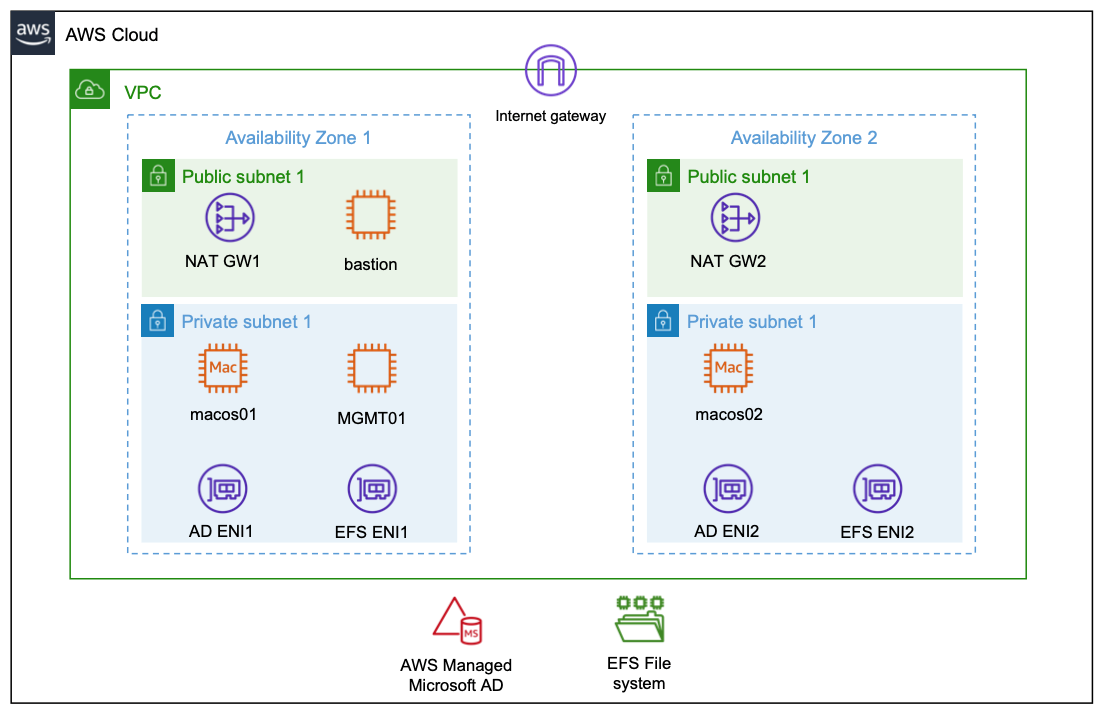
The solution is comprised of the following components:

• A VPC across two Availability Zones
• Two public subnets, two private app subnets, and two private DB subnets
• An Internet Gateway attached to the VPC
  • A public route table routing internet traffic to the Internet Gateway
  • Two private route tables routing traffic internally within the VPC
• A frontend web server application Elastic Load Balancing that routes traffic to the Apache Web Servers
• An Auto Scaling group that launches additional Apache Web Servers based on defined scaling policies. Each instance of the web server is based on a launch template, which defines the same configuration for each new web server.
• A hosted zone in Amazon Route 53 with a domain name that routes to the frontend web server Elastic Load Balancing
• An application Elastic Load Balancing that routes traffic to the Tomcat application servers
• An Auto Scaling group that launches additional Tomcat Application Servers based on defined scaling policies. Each instance of the Tomcat application server is based on a launch template, which defines the same configuration and software components for each new application server
• A Redis cache cluster with a primary and replica node to store session data after the user has authenticated, making your application servers stateless
• A Redis open-source Java client, with a Tomcat Session Manager implementation to store authenticated user session data in Redis cache
• A MySQL Amazon Relational Database Service (Amazon RDS) Multi-AZ deployment for MySQL RDS to store the contact management and role access tables
• An Amazon Simple Storage Service (Amazon S3) bucket to store the application and framework artifacts, images, scripts and configuration files that are referenced by any new Tomcat application server instances provisioned by automatic scaling
• Amazon Cognito with a sign-up Lambda function to register users and insert a corresponding entry in the user account tables. Cognito acts as an identity provider and performs the user authentication using an OpenID Connect Authenticator Java component

Walkthrough

The following steps overviews how to deploy the blog solution:

• Clone and build the Sample Web Application and AWS Signup Lambda Maven projects from GitHub repository
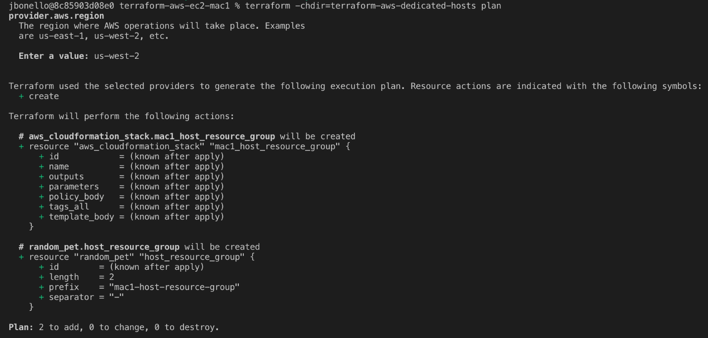
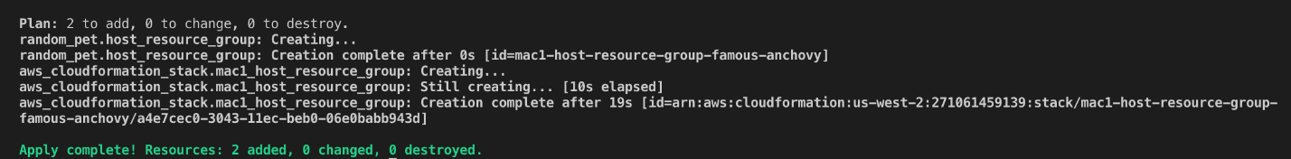
• Deploy the CloudFormation template (java-webapp-infra.yaml) to create the AWS networking infrastructure and the CloudFormation template (java-webapp-rds.yaml) to create the database instance
• Update and build the sample web application and signup Lambda function
• Upload the packages into your S3 bucket
• Deploy the CloudFormation template (java-webapp-components.yaml) to create the blog solution components
• Update the solution configuration files and upload them into your S3 bucket
• Run a script to provision the underlying database tables
• Validate the web application, session cache and automatic scaling functionality
• Clean up resources

Prerequisites

For this walkthrough, you should have the following prerequisites:

• An AWS account
• An Amazon Elastic Compute Cloud (Amazon EC2) key pair (required for authentication). For more details, see Amazon EC2 key pairs
• A Java Integrated Development Environment (IDE) such as Eclipse or NetBeans. AWS also offers a cloud-based IDE that lets you write, run and debug code in your browser without having to install files or configure your development machine, called AWS Cloud9. I will show how AWS Cloud9 can be used as part of a DevOps solution in a subsequent post
• A valid domain name and SSL certificate for the deployed web application. To validate the OAuth 2.0 integration, Cognito requires the URL that the user is redirected to after successful sign-in to be HTTPS. Refer to a configuring a user pool app client for more details
• Downloaded the following JARs:
  • apache-tomcat-9.0.41.tar.gz
  • tomcat-oidcauth-2.3.0-tomcat90
  • redisson-all-3.14.1.jar
  • redisson-tomcat-9-3.14.1

Note: the solution was validated in the preceding versions and therefore, the launch template created for the CloudFormation solution stack refers to these specific JARs. If you decide to use different versions, then the ‘java-webapp-components.yaml’ will need to be updated to reflect the new versions. Alternatively, you can externalize the parameters in the template.

Clone the GitHub repository to your local machine

This repository contains the sample code for the Java web application and post confirmation sign-up Lambda function. It also contains the CloudFormation templates required to set up the AWS infrastructure, SQL script to create the supporting database and configuration files for the web server, Tomcat application server and Redis cache.

Deploy infrastructure CloudFormation template

1. Log in to the AWS Management Console and open the CloudFormation service.

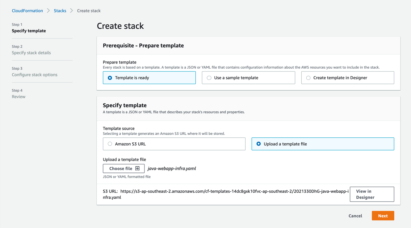
2. Create the infrastructure stack using the java-webapp-infra.yaml template (located in the ‘config’ directory of the repo).

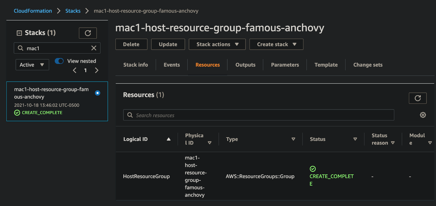
3. Infrastructure stack outputs:

Deploy database CloudFormation template

1.  Log in to the AWS Management Console and open the CloudFormation service.
2. Create the infrastructure stack using the java-webapp-rds.yaml template (located in the ‘config’ directory of the repo).
3. Database stack outputs.

Update and build sample web application and signup Lambda function

1. Import the ‘sample-webapp’ and ‘aws-signup-lambda’ Maven projects from the repository into your IDE.
2. Update the sample-webapp’s UserDAO class to reflect the RDSEndpoint, DBUserName, and DBPassword from the previous step:”

   // Externalize and update jdbcURL, jdbcUsername, jdbcPassword parameters specific to your environment
   	private String jdbcURL = "jdbc:mysql://<RDSEndpoint>:3306/webappdb?useSSL=false";
   	private String jdbcUsername = "<DBUserName>";
   	private String jdbcPassword = "<DBPassword>";

3. To build the ‘sample-webapp’ Maven project, use the standard ‘clean install’ goals.
4. Update the aws-signup-lambda’s signupHandler class to reflect RDSEndpoint, DBUserName, and DBPassword from the solution stack:

   // Update with your database connection details
   		String jdbcURL = "jdbc:mysql://<RDSEndpoint>:3306/webappdb?useSSL=false";
   		String jdbcUsername = "<DBUserName>";
   		String jdbcPassword = "<DBPassword>";

5. To build the aws-signup-lambda Maven project, use the ‘package shade:shade’ goals to include all dependencies in the package.
6. Two packages are created in their respective target directory: ‘sample-webapp.war’ and ‘create-user-lambda-1.0.jar’

Upload the packages into your S3 bucket

1. Log in to the AWS Management Console and open the S3 service.
2. Select the bucket created by the infrastructure CloudFormation template in an earlier step.

3.  Create a ‘config’ and ‘lib’ folder in the bucket.

4.  Upload the ‘sample-webapp.war’ and ‘create-user-lambda-1.0.jar’ created an earlier step (along with the downloaded packages from the pre-requisites section) into the ‘lib’ folder of the bucket. The ‘lib’ folder should look like this:

Note: the solution was validated in the preceding versions and therefore, the launch template created for the CloudFormation solution stack refers to these specific package names.

Deploy the solution components CloudFormation template

1.       Log in to the AWS Management Console and open the CloudFormation service (if you aren’t already logged in from the previous step).

2.       Create the web application solution stack using the ‘java-webapp-components.yaml’ template (located in the ‘config’ directory of the repo).

3.       Guidance on the different template input parameters:

a.       BastionSGSource – default is 0.0.0.0/0, but it is recommended to restrict this to your allowed IPv4 CIDR range for additional security

b.       BucketName – the bucket name created as part of the infrastructure stack. This blog uses the bucket name is ‘chanbi-java-webapp-bucket’

c.       CallbackURL – the URL that the user is redirected to after successful sign up/sign in is composed of your domain name (blog.example.com), the application root (sample-webapp), and the authentication form action ‘j_security_check’. As noted earlier, this needs to be over HTTPS

d.       CreateUserLambdaKey – the S3 object key for the signup Lambda package. This blog uses the key ‘lib/create-user-lambda-1.0.jar’

e.       DBUserName – the database user name for the MySQL RDS. Make note of this as it will be required in a subsequent step

f.        DBUserPassword – the database user password. Make note of this as it will be required in a subsequent step

g.       KeyPairName – the key pair to use when provisioning the EC2 instances. This key pair was created in the pre-requisite step

h.       WebALBSGSource – the IPv4 CIDR range allowed to access the web app. Default is 0.0.0.0/0

i.         The remaining parameters are import names from the infrastructure stack. Use default settings

4.       After successful stack creation, you should see the following java web application solution stack output:

Update configuration files

1. The GitHub repository’s ‘config’ folder contains the configuration files for the web server, Tomcat application server and Redis cache, which needs to be updated to reflect the parameters specific to your stack output in the previous step.
2. Update the virtual hosts in ‘httpd.conf’ to proxy web traffic to the internal app load balancer. Use the value defined by the key ‘AppALBLoadBalancerDNS’ from the stack output.

   <VirtualHost *:80>
   ProxyPass / http://<AppALBLoadBalancerDNS>:8080/
   ProxyPassReverse / http://<AppALBLoadBalancerDNS>:8080/
   </VirtualHost>

3. Update JDBC resource for the ‘webappdb’ in the ‘context.xml, with the values defined by the RDSEndpoint, DBUserName, and DBPassword from the solution components CloudFormation stack:

   <Resource name="jdbc/webappdb" auth="Container" type="javax.sql.DataSource"
                  maxTotal="100" maxIdle="30" maxWaitMillis="10000"
                  username="<DBUserName>" password="<DBPassword>" driverClassName="com.mysql.jdbc.Driver"
                  url="jdbc:mysql://<RDSEndpoint>:3306/webappdb"/>

4. Log in to the AWS Management Console and open the Amazon Cognito service. Select ‘Manage User Pools’ and you will notice that a ‘java-webapp-pool’ has been created by the solution components CloudFormation stack. Select the ‘java-webapp-pool’ and make note of the ‘Pool Id’, ‘App client id’ and ‘App client secret’.

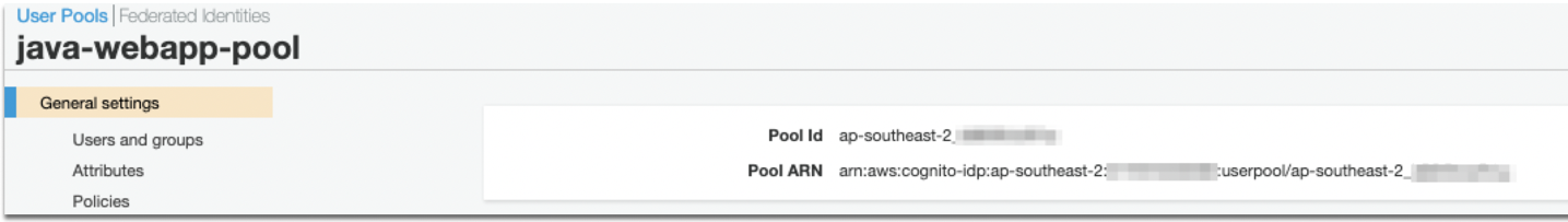
5.  Update ‘Valve’ configuration in the ‘context.xml’, with the ‘Pool Id’, ‘App client id’ and ‘App client secret’ values from the previous step. The Cognito IDP endpoint specific to your Region can be found here. The host base URI needs to be replaced with the domain for your web application.

    <Valve className="org.bsworks.catalina.authenticator.oidc.tomcat90.OpenIDConnectAuthenticator"
       providers="[
           {
               name: 'Amazon Cognito',
               issuer: https://<cognito-idp-endpoint-for-you-region>/<cognito-pool-id>,
               clientId: <user-pool-app-client-id>,
               clientSecret: <user-pool-app-client-secret>
           }
       ]"
        hostBaseURI="https://<your-sample-webapp-domain>" usernameClaim="email" />

6.  Update the ‘address’ parameter in ‘redisson.yaml’ with Redis cluster endpoint. Use the value defined by the key ‘RedisClusterEndpoint’ from the solution components CloudFormation stack output.

singleServerConfig:
    address: "redis://<RedisClusterEndpoint>:6379"

7.  No updates are required to the following files:

a.  server.xml – defines a data source realm for the user names, passwords, and roles assigned to users

      <Realm className="org.apache.catalina.realm.DataSourceRealm"
   dataSourceName="jdbc/webappdb" localDataSource="true"
   userTable="user_accounts" userNameCol="user_name" userCredCol="user_pass"
   userRoleTable="user_account_roles" roleNameCol="role_name" debug="9" />
      </Realm>

b.  tomcat.service – allows Tomcat to run as a service

c.  uninstall-sample-webapp.sh – removes the sample web application

Upload configuration files into your S3 bucket

1. Upload the configuration files from the previous step into the ‘config’ folder of the bucket. The ‘config’ folder should look like this:

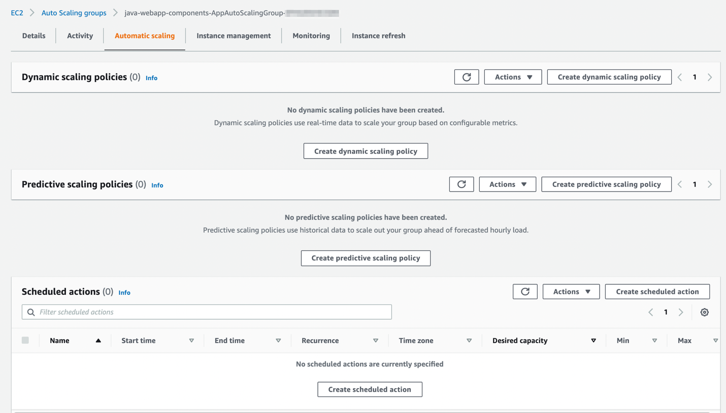
Update the Auto Scaling groups

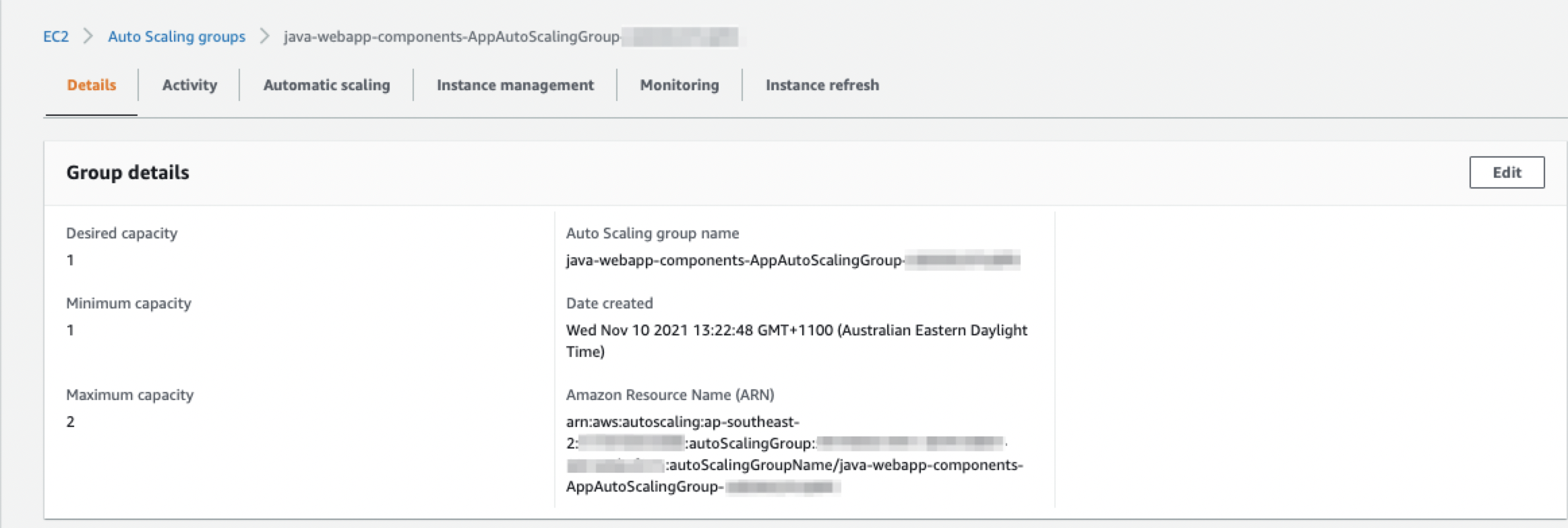
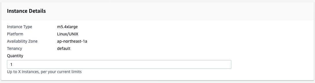
1. Auto Scaling groups manage the provisioning and removal of the web and application instances in our solution. To start an instance of the web server, update the Auto Scaling group’s desired capacity (1), minimum capacity (1) and maximum capacity (2) as shown in the following image:

2.  To start an instance of the application server, update the Auto Scaling group’s desired capacity (1), minimum capacity (1) and maximum capacity (2) for as shown in the following image:

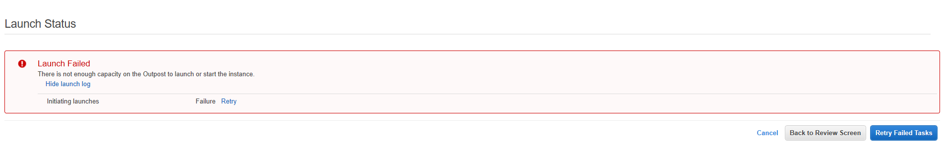
The web and application scaling groups will show a status of “Updating capacity” (as shown in the following image) as the instances start up.

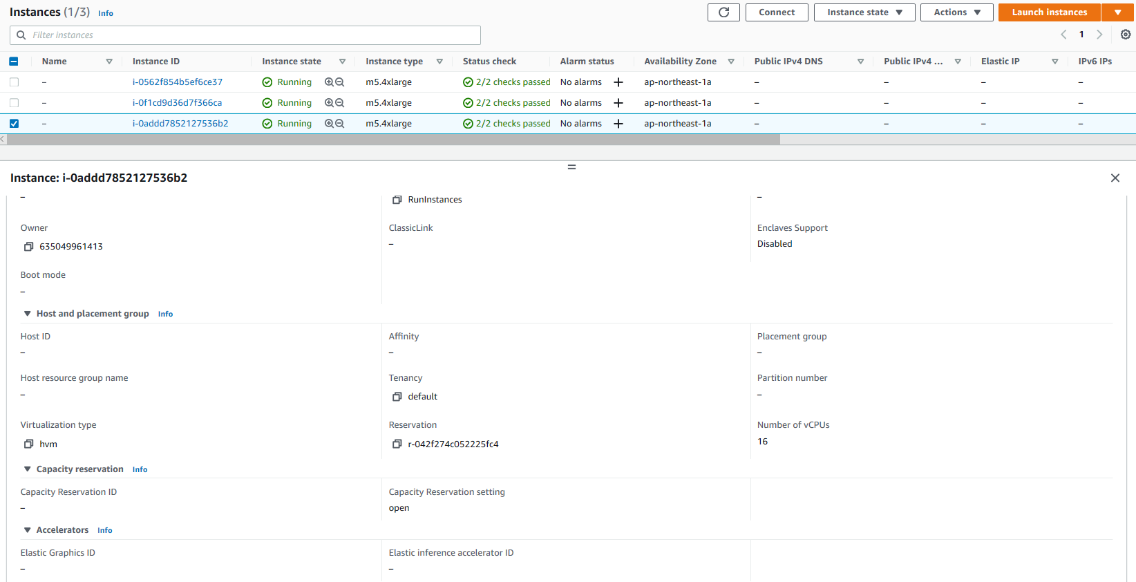
After web and application servers have started, an instance will appear under ‘Instance management’ with a ‘Healthy’ status for each Auto Scaling group (as shown in the following image).

Run the database script webappdb_create_tables.sql

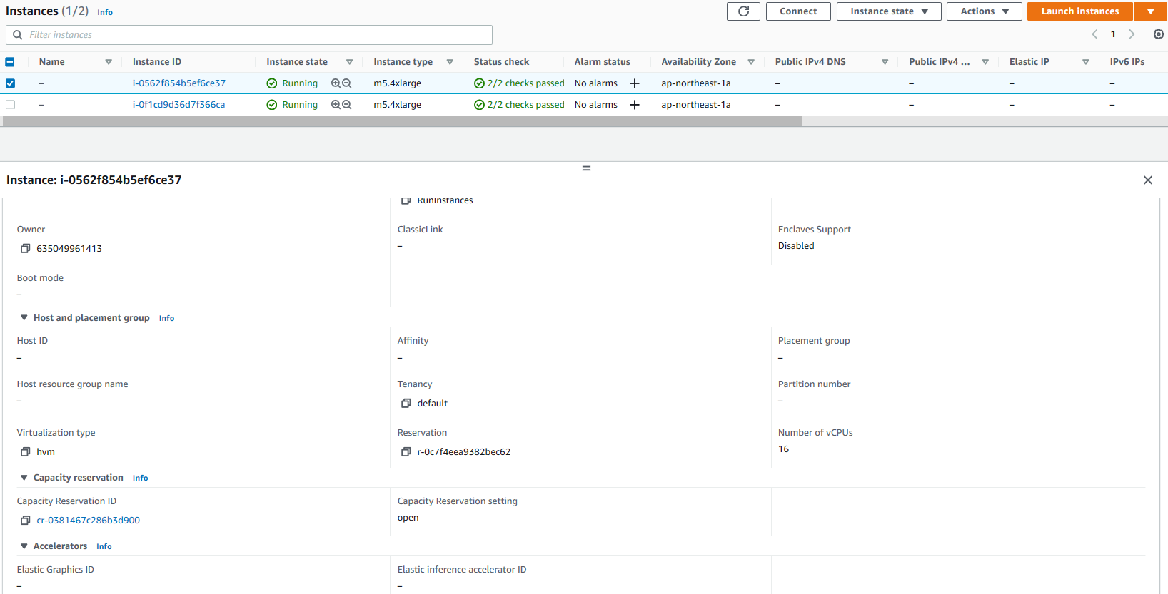
1. The database script creates the database and underlying tables required by the web application. As the database server resides in the DB private subnet and is only accessible from the application server instance, we need to first connect (via SSH) to the bastion host (using public IPv4 DNS), and from there we can connect (via SSH) to the application server instance (using its private IPv4 address). This will in turn allow us to connect to the database instance and run the database script. Refer to connecting to your Linux instance using SSH for more details. Instance details are located under the ‘Instances’ view (as shown in the following image).

2.  Transfer the database script webappdb_create_tables.sql to the application server instance via the Bastion Host. Refer to transferring files using a client for details.

3.  Once connected to the application server via SSH, execute the command to connect to the database instance:

mysql -h <RDSEndpoint> -P 3306 -u <DBUserName> -p

4. Enter the DB user password used when creating the database instance. You will be presented with the MySQL prompt after successful login:

Welcome to the MariaDB monitor.  Commands end with ; or \g.
Your MySQL connection id is 300
Server version: 8.0.23 Source distribution

Copyright (c) 2000, 2018, Oracle, MariaDB Corporation Ab and others.

Type 'help;' or '\h' for help. Type '\c' to clear the current input statement.

MySQL [(none)]>

5. Run the command to run the database script webappdb_create_tables.sql:

source /home/ec2-user/webappdb_create_tables.sql

Add an HTTPS listener to the external web load balancer

1. Log in to the AWS Management Console and select Load Balancers as part of the EC2 service
   
2. Add a HTTPS listener on port 443 for the web load balancer. The default action for the listener is to forward traffic to the web instance target group. Refer to create an HTTPS listener for your Application Load Balancer for more details.
   

Reference the SSL certificate for your domain. In the following example, I have used a certificate from AWS Certificate Manager (ACM) for my domain. You also have the option of using a certificate from Identity Access Management or importing your own certificate.

Update your DNS to route traffic from the external web load balancer

1. In this example, I use Amazon Route 53 as the Domain Name Server (DNS) service, but the steps will be similar when using your own DNS service.
2. Create an A record type that routes traffic from your domain name to the external web load balancer. For more details, refer to creating records by using the Amazon Route 53 console.
   

Validate the web application

1. In your browser, access the following https://<yourdomain.example.com>/sample-webapp
   
2. Select “Amazon Cognito” to authenticate using Cognito as the Identity Provider (IdP). You will be redirected to the login page for your Cognito domain.
   
3. Select the “Sign up” to create a new user and enter your email and password. Note the password strength requirements that can be configured as part of the user pool’s policies.
   
4. An email with the verification code will be sent to the sign-up email address. Enter the code on the verification code screen.
   
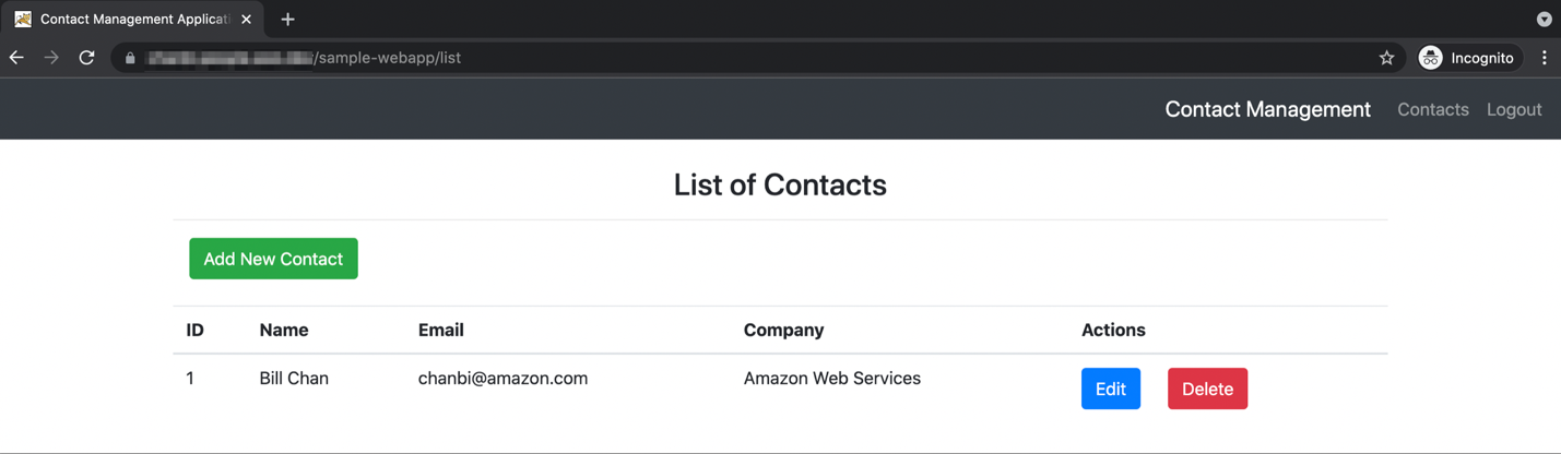
5. After successful confirmation, you will be re-directed to the authenticated landing page for the web application.
   
6. The simple web application allows you to add, edit, and delete contacts as shown in the following image.
   

Validate the session data on Redis

1. Follow the steps outlined in connecting to nodes for details on connecting to your Redis cache cluster. You will need to connect to your application server instance (via the bastion host) to perform this as the Redis cache is only accessible from the private subnet.
2. After successfully installing the Redis client, search for your authenticated user session key in the cluster by running the command (from within the ‘redis-stable’ directory):

   src/redis-cli -c -h <RedisClusterEndpoint> -p 6379 -–bigkeys

3. You should see an output with your Tomcat authenticated session (if you can’t, perform another login via the Cognito login screen):

   # Scanning the entire keyspace to find biggest keys as well as
   # average sizes per key type.  You can use -i 0.1 to sleep 0.1 sec
   # per 100 SCAN commands (not usually needed).
   
   [00.00%] Biggest hash   found so far '"redisson:tomcat_session:AE647D93F2BECEFEE07B5B42C435E3DE"' with 8 fields

4. Connect to the cache cluster:

   # src/redis-cli -c -h <RedisClusterEndpoint> -p 6379

5. Run the HGETALL command to get the session details:

   java-webapp-redis-cluster.<xxxxxx>.0001.apse2.cache.amazonaws.com:6379> HGETALL "redisson:tomcat_session:AE647D93F2BECEFEE07B5B42C435E3DE"
    1) "session:creationTime"
    2) "\x04L\x00\x00\x01}\x16\x92\x1bX"
    3) "session:lastAccessedTime"
    4) "\x04L\x00\x00\x01}\x16\x92%\x9c"
    5) "session:principal"
    6) "\x04\x04\t>@org.apache.catalina.realm.GenericPrincipal$SerializablePrincipal\x00\x00\x00\x00\x00\x00\x00\x01\x00\x00\x00\x04>\x04name\x16\x00>\bpassword\x16\x00>\tprincipal\x16\x00>\x05roles\x16\x00\x16>\[email protected]>\[email protected]\x01B\x01\x14>\bstandard"
    7) "session:maxInactiveInterval"
    8) "\x04K\x00\x00\a\b"
    9) "session:isValid"
   10) "\x04P"
   11) "session:authtype"
   12) "\x04>\x04FORM"
   13) "session:isNew"
   14) "\x04Q"
   15) "session:thisAccessedTime"
   16) "\x04L\x00\x00\x01}\x16\x92%\x9c"

Scale your web and application server instances

1. Amazon EC2 Auto Scaling provides several ways for you to scale instances in your Auto Scaling group such as scaling manually as we did in an earlier step. But you also have the option to scale dynamically to meet changes in demand (such as maintaining CPU Utilization at 50%), predictively scale in advance of daily and weekly patterns in traffic flows, or scale based on a scheduled time. Refer to scaling the size of your Auto Scaling group for more details.
   
2. We will create a scheduled action to provision another application server instance.
   
3. As per our scheduled action, at 11.30 am, an additional application server instance is started.
   
4. Under instance management, you will see an additional instance in ‘Pending’ state as it starts.
   
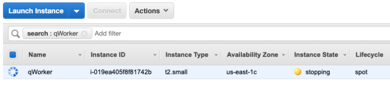
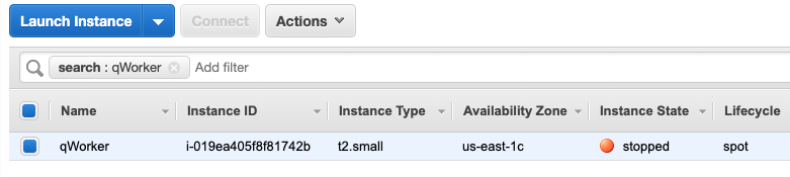
5. To test the stateless nature of your application, you can manually stop the original application server instance and observe that your end-user experience is unaffected i.e. you are not prompted to re-authenticate and can continue using the application as your session data is stored in Redis ElastiCache and not tied to the original instance.

Cleaning up

To avoid incurring future charges, remove the resources by deleting the java-webapp-components, java-webapp-rds and java-webapp-infra CloudFormation stacks.

Conclusion

Customers with significant investments in Java application server technologies have options to migrate to the cloud without requiring a complete re-architecture of their applications. In this blog, we’ve shown an approach to modernizing Java applications running on Tomcat Application Server in AWS. And in doing so, take advantage of cloud-native features such as automatic scaling, provisioning infrastructure as code, and leveraging managed services (such as ElastiCache for Redis and Amazon RDS) to make our application stateless. We also demonstrated modernization features such as authentication and user provisioning via an external IdP (Amazon Cognito). For more information on different re-platforming patterns refer to the AWS Prescriptive Guidance on Migration.