How Netflix’s Container Platform Connects Linux Kernel Panics to Kubernetes Pods
By Kyle Anderson
With a recent effort to reduce customer (engineers, not end users) pain on our container platform Titus, I started investigating “orphaned” pods. There are pods that never got to finish and had to be garbage collected with no real satisfactory final status. Our Service job (think ReplicatSet) owners don’t care too much, but our Batch users care a lot. Without a real return code, how can they know if it is safe to retry or not?
These orphaned pods represent real pain for our users, even if they are a small percentage of the total pods in the system. Where are they going, exactly? Why did they go away?
This blog post shows how to connect the dots from the worst case scenario (a kernel panic) through to Kubernetes (k8s) and eventually up to us operators so that we can track how and why our k8s nodes are going away.
Where Do Orphaned Pods Come From?
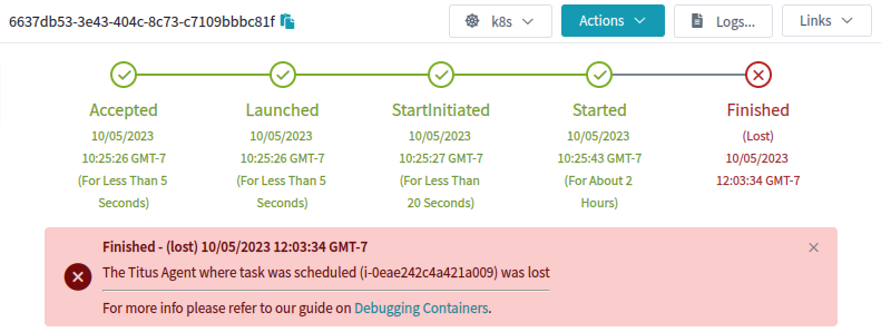
Orphaned pods get lost because the underlying k8s node object goes away. Once that happens a GC process deletes the pod. On Titus we run a custom controller to store the history of Pod and Node objects, so that we can save some explanation and show it to our users. This failure mode looks like this in our UI:
What it looks like to our users when a k8s node and its pods disappear
This is an explanation, but it wasn’t very satisfying to me or to our users. Why was the agent lost?
Where Do Lost Nodes Come From?
Nodes can go away for any reason, especially in “the cloud”. When this happens, usually a k8s cloud-controller provided by the cloud vendor will detect that the actual server, in our case an EC2 Instance, has actually gone away, and will in turn delete the k8s node object. That still doesn’t really answer the question of why.
How can we make sure that every instance that goes away has a reason, account for that reason, and bubble it up all the way to the pod? It all starts with an annotation:
Just making a place to put this data is a great start. Now all we have to do is make our GC controllers aware of this annotation, and then sprinkle it into any process that could potentially make a pod or node go away unexpectedly. Adding an annotation (as opposed to patching the status) preserves the rest of the pod as-is for historical purposes. (We also add annotations for what did the terminating, and a short reason-code for tagging)
The pod-termination-reason annotation is useful to populate human readable messages like:
“This pod was preempted by a higher priority job ($id)”
“This pod had to be terminated because the underlying hardware failed ($failuretype)”
“This pod had to be terminated because $user ran sudo halt on the node”
“This pod died unexpectedly because the underlying node kernel panicked!”
But wait, how are we going to annotate a pod for a node that kernel panicked?
Capturing Kernel Panics
When the Linux kernel panics, there is just not much you can do. But what if you could send out some sort of “with my final breath, I curse Kubernetes!” UDP packet?
Inspired by this Google Spanner paper, where Spanner nodes send out a “last gasp” UDP packet to release leases & locks, you too can configure your servers to do the same upon kernel panic using a stock Linux module: netconsole.
Configuring Netconsole
The fact that the Linux kernel can even send out UDP packets with the string ‘kernel panic’, while it is panicking, is kind of amazing. This works because netconsole needs to be configured with almost the entire IP header filled out already beforehand. That is right, you have to tell Linux exactly what your source MAC, IP, and UDP Port are, as well as the destination MAC, IP, and UDP ports. You are practically constructing the UDP packet for the kernel. But, with that prework, when the time comes, the kernel can easily construct the packet and get it out the (preconfigured) network interface as things come crashing down. Luckily the netconsole-setup command makes the setup pretty easy. All the configuration options can be set dynamically as well, so that when the endpoint changes one can point to the new IP.
Once this is setup, kernel messages will start flowing right after modprobe. Imagine the whole thing operating like a dmesg | netcat -u $destination 6666, but in kernel space.
Netconsole “Last Gasp” Packets
With netconsole setup, the last gasp from a crashing kernel looks like a set of UDP packets exactly like one might expect, where the data of the UDP packet is simply the text of the kernel message. In the case of a kernel panic, it will look something like this (one UDP packet per line):
The last piece is to connect is Kubernetes (k8s). We need a k8s controller to do the following:
Listen for netconsole UDP packets on port 6666, watching for things that look like kernel panics from nodes.
Upon kernel panic, lookup the k8s node object associated with the IP address of the incoming netconsole packet.
For that k8s node, find all the pods bound to it, annotate, then delete those pods (they are toast!).
For that k8s node, annotate the node and then delete it too (it is also toast!).
Parts 1&2 might look like this:
for {
    n, addr, err := serverConn.ReadFromUDP(buf)
    if err != nil {
        klog.Errorf("Error ReadFromUDP: %s", err)
    } else {
        line := santizeNetConsoleBuffer(buf[0:n])
        if isKernelPanic(line) {
            panicCounter = 20
            go handleKernelPanicOnNode(ctx, addr, nodeInformer, podInformer, kubeClient, line)
        }
    }
    if panicCounter > 0 {
        klog.Infof("KernelPanic context from %s: %s", addr.IP, line)
        panicCounter++
    }
}
And then parts 3&4 might look like this:
func handleKernelPanicOnNode(ctx context.Context, addr *net.UDPAddr, nodeInformer cache.SharedIndexInformer, podInformer cache.SharedIndexInformer, kubeClient kubernetes.Interface, line string) {
    node := getNodeFromAddr(addr.IP.String(), nodeInformer)
    if node == nil {
        klog.Errorf("Got a kernel panic from %s, but couldn't find a k8s node object for it?", addr.IP.String())
    } else {
        pods := getPodsFromNode(node, podInformer)
        klog.Infof("Got a kernel panic from node %s, annotating and deleting all %d pods and that node.", node.Name, len(pods))
        annotateAndDeletePodsWithReason(ctx, kubeClient, pods, line)
        err := deleteNode(ctx, kubeClient, node.Name)
        if err != nil {
            klog.Errorf("Error deleting node %s: %s", node.Name, err)
        } else {
            klog.Infof("Deleted panicked node %s", node.Name)
        }
    }
}
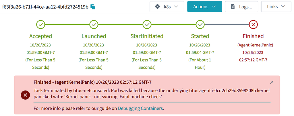
With that code in place, as soon as a kernel panic is detected, the pods and nodes immediately go away. No need to wait for any GC process. The annotations help document what happened to the node & pod:
A real pod lost on a real k8s node that had a real kernel panic!
Conclusion
Marking that a job failed because of a kernel panic may not be that satisfactory to our customers. But they can take satisfaction in knowing that we now have the required observability tools to start fixing those kernel panics!
Do you also enjoy really getting to the bottom of why things fail in your systems or think kernel panics are cool? Join us on the Compute Team where we are building a world-class container platform for our engineers.
The Compute team at Netflix is charged with managing all AWS and containerized workloads at Netflix, including autoscaling, deployment of containers, issue remediation, etc. As part of this team, I work on fixing strange things that users report.
This particular issue involved a custom internal FUSE filesystem: ndrive. It had been festering for some time, but needed someone to sit down and look at it in anger. This blog post describes how I poked at /procto get a sense of what was going on, before posting the issue to the kernel mailing list and getting schooled on how the kernel’s wait code actually works!
Here, our management engine has made an HTTP call to the Docker API’s unix socket asking it to kill a container. Our containers are configured to be killed via SIGKILL. But this is strange. kill(SIGKILL) should be relatively fatal, so what is the container doing?
$ docker exec -it 6643cd073492 bash
OCI runtime exec failed: exec failed: container_linux.go:380: starting container process caused: process_linux.go:130: executing setns process caused: exit status 1: unknown
Hmm. Seems like it’s alive, but setns(2) fails. Why would that be? If we look at the process tree via ps awwfux, we see:
It is in the process of exiting, but it seems stuck. The only child is the ndrive process in Z (i.e. “zombie”) state, though. Zombies are processes that have successfully exited, and are waiting to be reaped by a corresponding wait() syscall from their parents. So how could the kernel be stuck waiting on a zombie?
# ls /proc/1544450/task
1544450  1544574
Ah ha, there are two threads in the thread group. One of them is a zombie, maybe the other one isn’t:
Indeed it is not a zombie. It is trying to become one as hard as it can, but it’s blocking inside FUSE for some reason. To find out why, let’s look at some kernel code. If we look at zap_pid_ns_processes(), it does:
/*
 * Reap the EXIT_ZOMBIE children we had before we ignored SIGCHLD.
 * kernel_wait4() will also block until our children traced from the
 * parent namespace are detached and become EXIT_DEAD.
 */
do {
        clear_thread_flag(TIF_SIGPENDING);
        rc = kernel_wait4(-1, NULL, __WALL, NULL);
} while (rc != -ECHILD);
which is where we are stuck, but before that, it has done:
/* Don't allow any more processes into the pid namespace */
disable_pid_allocation(pid_ns);
which is why docker can’t setns() — the namespace is a zombie. Ok, so we can’t setns(2), but why are we stuck in kernel_wait4()? To understand why, let’s look at what the other thread was doing in FUSE’s request_wait_answer():
/*
 * Either request is already in userspace, or it was forced.
 * Wait it out.
 */
wait_event(req->waitq, test_bit(FR_FINISHED, &req->flags));
Ok, so we’re waiting for an event (in this case, that userspace has replied to the FUSE flush request). But zap_pid_ns_processes()sent a SIGKILL! SIGKILL should be very fatal to a process. If we look at the process, we can indeed see that there’s a pending SIGKILL:
Viewing process status this way, you can see 0x100 (i.e. the 9th bit is set) under SigPnd, which is the signal number corresponding to SIGKILL. Pending signals are signals that have been generated by the kernel, but have not yet been delivered to userspace. Signals are only delivered at certain times, for example when entering or leaving a syscall, or when waiting on events. If the kernel is currently doing something on behalf of the task, the signal may be pending. Signals can also be blocked by a task, so that they are never delivered. Blocked signals will show up in their respective pending sets as well. However, man 7 signal says: “The signals SIGKILL and SIGSTOP cannot be caught, blocked, or ignored.” But here the kernel is telling us that we have a pending SIGKILL, aka that it is being ignored even while the task is waiting!
Red Herring: How do Signals Work?
Well that is weird. The wait code (i.e. include/linux/wait.h) is used everywhere in the kernel: semaphores, wait queues, completions, etc. Surely it knows to look for SIGKILLs. So what does wait_event() actually do? Digging through the macro expansions and wrappers, the meat of it is:
So it loops forever, doing prepare_to_wait_event(), checking the condition, then checking to see if we need to interrupt. Then it does cmd, which in this case is schedule(), i.e. “do something else for a while”. prepare_to_wait_event() looks like:
long prepare_to_wait_event(struct wait_queue_head *wq_head, struct wait_queue_entry *wq_entry, int state) { unsigned long flags; long ret = 0;
spin_lock_irqsave(&wq_head->lock, flags); if (signal_pending_state(state, current)) { /* * Exclusive waiter must not fail if it was selected by wakeup, * it should "consume" the condition we were waiting for. * * The caller will recheck the condition and return success if * we were already woken up, we can not miss the event because * wakeup locks/unlocks the same wq_head->lock. * * But we need to ensure that set-condition + wakeup after that * can't see us, it should wake up another exclusive waiter if * we fail. */ list_del_init(&wq_entry->entry); ret = -ERESTARTSYS; } else { if (list_empty(&wq_entry->entry)) { if (wq_entry->flags & WQ_FLAG_EXCLUSIVE) __add_wait_queue_entry_tail(wq_head, wq_entry); else __add_wait_queue(wq_head, wq_entry); } set_current_state(state); } spin_unlock_irqrestore(&wq_head->lock, flags);
It looks like the only way we can break out of this with a non-zero exit code is if signal_pending_state() is true. Since our call site was just wait_event(), we know that state here is TASK_UNINTERRUPTIBLE; the definition of signal_pending_state() looks like:
static inline int signal_pending_state(unsigned int state, struct task_struct *p) { if (!(state & (TASK_INTERRUPTIBLE | TASK_WAKEKILL))) return 0; if (!signal_pending(p)) return 0;
Our task is not interruptible, so the first if fails. Our task should have a signal pending, though, right?
static inline int signal_pending(struct task_struct *p)
{
        /*
         * TIF_NOTIFY_SIGNAL isn't really a signal, but it requires the same
         * behavior in terms of ensuring that we break out of wait loops
         * so that notify signal callbacks can be processed.
         */
        if (unlikely(test_tsk_thread_flag(p, TIF_NOTIFY_SIGNAL)))
                return 1;
        return task_sigpending(p);
}
As the comment notes, TIF_NOTIFY_SIGNAL isn’t relevant here, in spite of its name, but let’s look at task_sigpending():
static inline int task_sigpending(struct task_struct *p)
{
        return unlikely(test_tsk_thread_flag(p,TIF_SIGPENDING));
}
Hmm. Seems like we should have that flag set, right? To figure that out, let’s look at how signal delivery works. When we’re shutting down the pid namespace in zap_pid_ns_processes(), it does:
Using PIDTYPE_MAX here as the type is a little weird, but it roughly indicates “this is very privileged kernel stuff sending this signal, you should definitely deliver it”. There is a bit of unintended consequence here, though, in that __send_signal_locked() ends up sending the SIGKILL to the shared set, instead of the individual task’s set. If we look at the __fatal_signal_pending() code, we see:
But it turns out this is a bit of a red herring (althoughittookawhile for me to understand that).
How Signals Actually Get Delivered To a Process
To understand what’s really going on here, we need to look at complete_signal(), since it unconditionally adds a SIGKILL to the task’s pending set:
sigaddset(&t->pending.signal, SIGKILL);
but why doesn’t it work? At the top of the function we have:
/*
 * Now find a thread we can wake up to take the signal off the queue.
 *
 * If the main thread wants the signal, it gets first crack.
 * Probably the least surprising to the average bear.
 */
if (wants_signal(sig, p))
        t = p;
else if ((type == PIDTYPE_PID) || thread_group_empty(p))
        /*
         * There is just one thread and it does not need to be woken.
         * It will dequeue unblocked signals before it runs again.
         */
        return;
but as Eric Biederman described, basically every thread can handle a SIGKILL at any time. Here’s wants_signal():
So… if a thread is already exiting (i.e. it has PF_EXITING), it doesn’t want a signal. Consider the following sequence of events:
1. a task opens a FUSE file, and doesn’t close it, then exits. During that exit, the kernel dutifully calls do_exit(), which does the following:
exit_signals(tsk); /* sets PF_EXITING */
2. do_exit() continues on to exit_files(tsk);, which flushes all files that are still open, resulting in the stack trace above.
3. the pid namespace exits, and enters zap_pid_ns_processes(), sends a SIGKILL to everyone (that it expects to be fatal), and then waits for everyone to exit.
4. this kills the FUSE daemon in the pid ns so it can never respond.
5. complete_signal() for the FUSE task that was already exiting ignores the signal, since it has PF_EXITING.
6. Deadlock. Without manually aborting the FUSE connection, things will hang forever.
Solution: don’t wait!
It doesn’t really make sense to wait for flushes in this case: the task is dying, so there’s nobody to tell the return code of flush() to. It also turns out that this bug can happen with several filesystems (anything that calls the kernel’s wait code in flush(), i.e. basically anything that talks to something outside the local kernel).
Individual filesystems will need to be patched in the meantime, for example the fix for FUSE is here, which was released on April 23 in Linux 6.3.
While this blog post addresses FUSE deadlocks, there are definitely issues in the nfs code and elsewhere, which we have not hit in production yet, but almost certainly will. You can also see it as a symptom of other filesystem bugs. Something to look out for if you have a pid namespace that won’t exit.
This is just a small taste of the variety of strange issues we encounter running containers at scale at Netflix. Our team is hiring, so please reach out if you also love red herrings and kernel deadlocks!
Have you noticed how simple questions sometimes lead to complex answers? Today we will tackle one such question. Category: our favorite – Linux networking.
When can two TCP sockets share a local address?
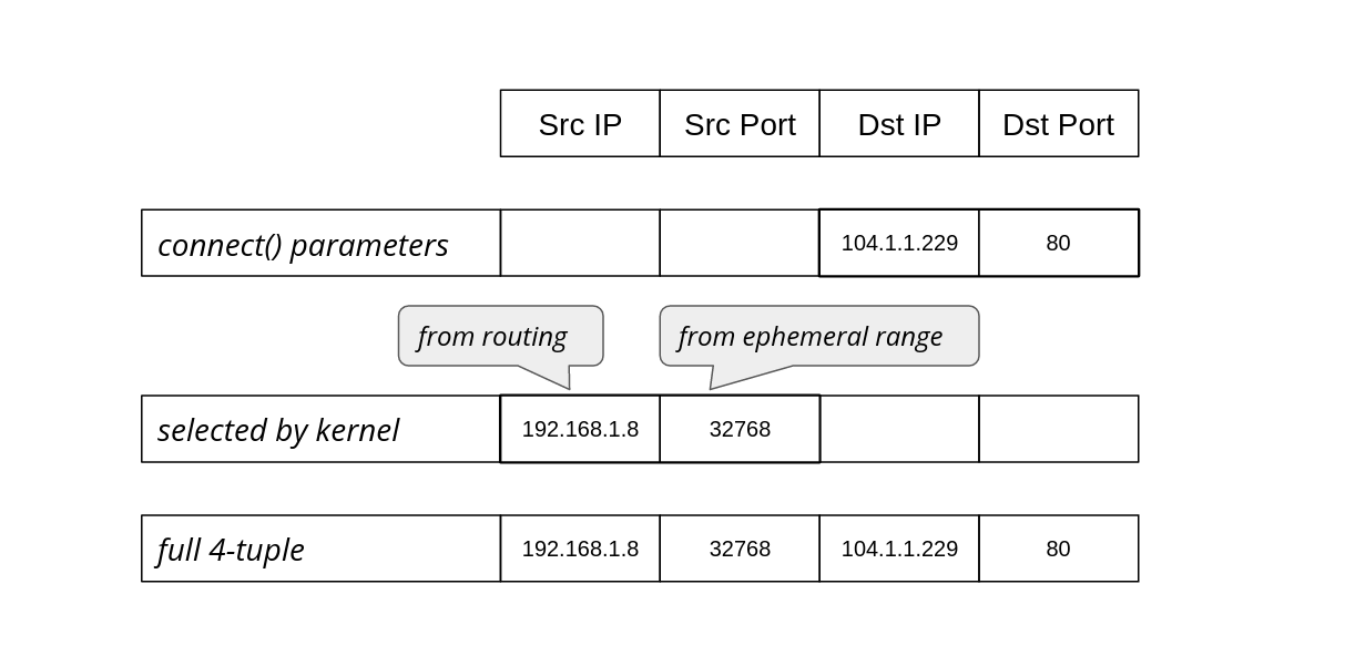
If I navigate to https://blog.cloudflare.com/, my browser will connect to a remote TCP address, might be 104.16.132.229:443 in this case, from the local IP address assigned to my Linux machine, and a randomly chosen local TCP port, say 192.0.2.42:54321. What happens if I then decide to head to a different site? Is it possible to establish another TCP connection from the same local IP address and port?
To find the answer let’s do a bit of learning by discovering. We have prepared eight quiz questions. Each will let you discover one aspect of the rules that govern local address sharing between TCP sockets under Linux. Fair warning, it might get a bit mind-boggling.
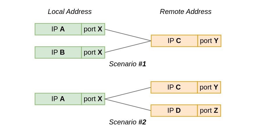
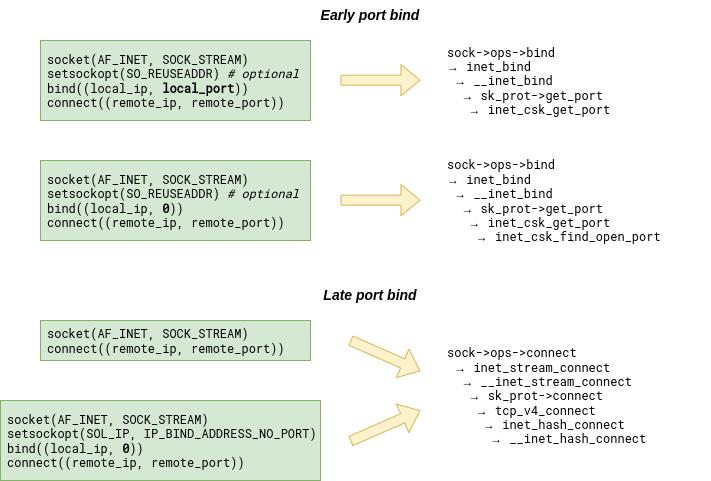
Questions are split into two groups by test scenario:
In the first test scenario, two sockets connect from the same local port to the same remote IP and port. However, the local IP is different for each socket.
While, in the second scenario, the local IP and port is the same for all sockets, but the remote address, or actually just the IP address, differs.
In our quiz questions, we will either:
let the OS automatically select the the local IP and/or port for the socket, or
Because we will be examining corner cases in the bind() logic, we need a way to exhaust available local addresses, that is (IP, port) pairs. We could just create lots of sockets, but it will be easier to tweak the system configuration and pretend that there is just one ephemeral local port, which the OS can assign to sockets:
Each quiz question is a short Python snippet. Your task is to predict the outcome of running the code. Does it succeed? Does it fail? If so, what fails? Asking ChatGPT is not allowed 😉
There is always a common setup procedure to keep in mind. We will omit it from the quiz snippets to keep them short:
from os import system
from socket import *

# Missing constants
IP_BIND_ADDRESS_NO_PORT = 24

# Our network namespace has just *one* ephemeral port
system("sysctl -w net.ipv4.ip_local_port_range='60000 60000'")

# Open a listening socket at *:1234. We will connect to it.
ln = socket(AF_INET, SOCK_STREAM)
ln.bind(("", 1234))
ln.listen(SOMAXCONN)
With the formalities out of the way, let us begin. Ready. Set. Go!
Scenario #1: When the local IP is unique, but the local port is the same
In Scenario #1 we connect two sockets to the same remote address – 127.9.9.9:1234. The sockets will use different local IP addresses, but is it enough to share the local port?
local IP
local port
remote IP
remote port
unique
same
same
same
127.0.0.1 127.1.1.1 127.2.2.2
60_000
127.9.9.9
1234
Quiz #1
On the local side, we bind two sockets to distinct, explicitly specified IP addresses. We will allow the OS to select the local port. Remember: our local ephemeral port range contains just one port (60,000).
Here, the setup is almost identical as before. However, we ask the OS to select the local IP address and port for the first socket. Do you think the result will differ from the previous question?
This quiz question is just like the one above. We just changed the ordering. First, we connect a socket from an explicitly specified local address. Then we ask the system to select a local address for us. Obviously, such an ordering change should not make any difference, right?
Scenario #2: When the local IP and port are the same, but the remote IP differs
In Scenario #2 we reverse our setup. Instead of multiple local IP’s and one remote address, we now have one local address 127.0.0.1:60000 and two distinct remote addresses. The question remains the same – can two sockets share the local port? Reminder: ephemeral port range is still of size one.
local IP
local port
remote IP
remote port
same
same
unique
same
127.0.0.1
60_000
127.8.8.8 127.9.9.9
1234
Quiz #4
Let’s start from the basics. We connect() to two distinct remote addresses. This is a warm up 🙂
Just when you thought it couldn’t get any weirder, we add SO_REUSEADDR into the mix.
First, we ask the OS to allocate a local address for us. Then we explicitly bind to the same local address, which we know the OS must have assigned to the first socket. We enable local address reuse for both sockets. Is this allowed?
Is it all clear now? Well, probably no. It feels like reverse engineering a black box. So what is happening behind the scenes? Let’s take a look.
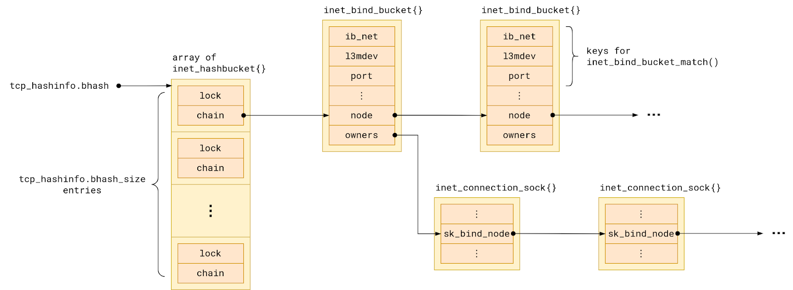
Linux tracks all TCP ports in use in a hash table named bhash. Not to be confused with with ehash table, which tracks sockets with both local and remote address already assigned.
Each hash table entry points to a chain of so-called bind buckets, which group together sockets which share a local port. To be precise, sockets are grouped into buckets by:
But in the simplest possible setup – single network namespace, no VRFs – we can say that sockets in a bind bucket are grouped by their local port number.
The set of sockets in each bind bucket, that is sharing a local port, is backed by a linked list named owners.
When we ask the kernel to assign a local address to a socket, its task is to check for a conflict with any existing socket. That is because a local port number can be shared only under some conditions:
/* There are a few simple rules, which allow for local port reuse by
 * an application.  In essence:
 *
 *   1) Sockets bound to different interfaces may share a local port.
 *      Failing that, goto test 2.
 *   2) If all sockets have sk->sk_reuse set, and none of them are in
 *      TCP_LISTEN state, the port may be shared.
 *      Failing that, goto test 3.
 *   3) If all sockets are bound to a specific inet_sk(sk)->rcv_saddr local
 *      address, and none of them are the same, the port may be
 *      shared.
 *      Failing this, the port cannot be shared.
 *
 * The interesting point, is test #2.  This is what an FTP server does
 * all day.  To optimize this case we use a specific flag bit defined
 * below.  As we add sockets to a bind bucket list, we perform a
 * check of: (newsk->sk_reuse && (newsk->sk_state != TCP_LISTEN))
 * As long as all sockets added to a bind bucket pass this test,
 * the flag bit will be set.
 * ...
 */
The comment above hints that the kernel tries to optimize for the happy case of no conflict. To this end the bind bucket holds additional state which aggregates the properties of the sockets it holds:
Let’s focus our attention just on the first aggregate property – fastreuse. It has existed since, now prehistoric, Linux 2.1.90pre1. Initially in the form of a bit flag, as the comment says, only to evolve to a byte-sized field over time.
The other six fields came on much later with the introduction of SO_REUSEPORT in Linux 3.9. Because they play a role only when there are sockets with the SO_REUSEPORT flag set. We are going to ignore them today.
Whenever the Linux kernel needs to bind a socket to a local port, it first has to look for the bind bucket for that port. What makes life a bit more complicated is the fact that the search for a TCP bind bucket exists in two places in the kernel. The bind bucket lookup can happen early – at bind() time – or late – at connect() – time. Which one gets called depends on how the connected socket has been set up:
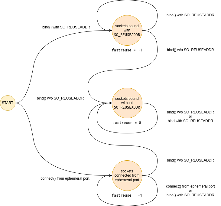
However, whether we land in inet_csk_get_port or __inet_hash_connect, we always end up walking the bucket chain in the bhash looking for the bucket with a matching port number. The bucket might already exist or we might have to create it first. But once it exists, its fastreuse field is in one of three possible states: -1, 0, or +1. As if Linux developers were inspired by quantum mechanics.
That state reflects two aspects of the bind bucket:
What sockets are in the bucket?
When can the local port be shared?
So let us try to decipher the three possible fastreuse states then, and what they mean in each case.
First, what does the fastreuse property say about the owners of the bucket, that is the sockets using that local port?
fastreuse is
owners list contains
-1
sockets connect()’ed from an ephemeral port
0
sockets bound without SO_REUSEADDR
+1
sockets bound with SO_REUSEADDR
While this is not the whole truth, it is close enough for now. We will soon get to the bottom of it.
When it comes port sharing, the situation is far less straightforward:
yes IFF local IP is unique OR conflicting socket uses SO_REUSEADDR ①
← idem
yes ②
connect() from the same ephemeral port to the same remote (IP, port)
yes IFF local IP unique ③
no ③
no ③
connect() from the same ephemeral port to a unique remote (IP, port)
yes ③
no ③
no ③
① Determined by inet_csk_bind_conflict() called from inet_csk_get_port() (specific port bind) or inet_csk_get_port() → inet_csk_find_open_port() (ephemeral port bind).
③ Because inet_hash_connect() → __inet_hash_connect()skips buckets with fastreuse != -1.
While it all looks rather complicated at first sight, we can distill the table above into a few statements that hold true, and are a bit easier to digest:
bind(), or early local address allocation, always succeeds if there is no local IP address conflict with any existing socket,
connect(), or late local address allocation, always fails when TCP bind bucket for a local port is in any state other than fastreuse = -1,
connect() only succeeds if there is no local and remote address conflict,
SO_REUSEADDR socket option allows local address sharing, if all conflicting sockets also use it (and none of them is in the listening state).
This is crazy. I don’t believe you.
Fortunately, you don’t have to. With drgn, the programmable debugger, we can examine the bind bucket state on a live kernel:
#!/usr/bin/env drgn

"""
dump_bhash.py - List all TCP bind buckets in the current netns.

Script is not aware of VRF.
"""

import os

from drgn.helpers.linux.list import hlist_for_each, hlist_for_each_entry
from drgn.helpers.linux.net import get_net_ns_by_fd
from drgn.helpers.linux.pid import find_task


def dump_bind_bucket(head, net):
    for tb in hlist_for_each_entry("struct inet_bind_bucket", head, "node"):
        # Skip buckets not from this netns
        if tb.ib_net.net != net:
            continue

        port = tb.port.value_()
        fastreuse = tb.fastreuse.value_()
        owners_len = len(list(hlist_for_each(tb.owners)))

        print(
            "{:8d}  {:{sign}9d}  {:7d}".format(
                port,
                fastreuse,
                owners_len,
                sign="+" if fastreuse != 0 else " ",
            )
        )


def get_netns():
    pid = os.getpid()
    task = find_task(prog, pid)
    with open(f"/proc/{pid}/ns/net") as f:
        return get_net_ns_by_fd(task, f.fileno())


def main():
    print("{:8}  {:9}  {:7}".format("TCP-PORT", "FASTREUSE", "#OWNERS"))

    tcp_hashinfo = prog.object("tcp_hashinfo")
    net = get_netns()

    # Iterate over all bhash slots
    for i in range(0, tcp_hashinfo.bhash_size):
        head = tcp_hashinfo.bhash[i].chain
        # Iterate over bind buckets in the slot
        dump_bind_bucket(head, net)


main()
Let’s take this script for a spin and try to confirm what Table 1 claims to be true. Keep in mind that to produce the ipython --classic session snippets below I’ve used the same setup as for the quiz questions.
Two connected sockets sharing ephemeral port 60,000:
With such tooling, proving that Table 2 holds true is just a matter of writing a bunch of exploratory tests.
But what has happened in that last snippet? The bind bucket has clearly transitioned from one fastreuse state to another. This is what Table 1 fails to capture. And it means that we still don’t have the full picture.
We have yet to find out when the bucket’s fastreuse state can change. This calls for a state machine.
Das State Machine
As we have just seen, a bind bucket does not need to stay in the initial fastreuse state throughout its lifetime. Adding sockets to the bucket can trigger a state change. As it turns out, it can only transition into fastreuse = 0, if we happen to bind() a socket that:
Now that we have the full picture, this begs the question…
Why are you telling me all this?
Firstly, so that the next time bind() syscall rejects your request with EADDRINUSE, or connect() refuses to cooperate by throwing the EADDRNOTAVAIL error, you will know what is happening, or at least have the tools to find out.
Secondly, because we have previously advertised a technique for opening connections from a specific range of ports which involves bind()’ing sockets with the SO_REUSEADDR option. What we did not realize back then, is that there exists a corner case when the same port can’t be shared with the regular, connect()‘ed sockets. While that is not a deal-breaker, it is good to understand the consequences.
To make things better, we have worked with the Linux community to extend the kernel API with a new socket option that lets the user specify the local port range. The new option will be available in the upcoming Linux 6.3. With it we no longer have to resort to bind()-tricks. This makes it possible to yet again share a local port with regular connect()‘ed sockets.
Closing thoughts
Today we posed a relatively straightforward question – when can two TCP sockets share a local address? – and worked our way towards an answer. An answer that is too complex to compress it into a single sentence. What is more, it’s not even the full answer. After all, we have decided to ignore the existence of the SO_REUSEPORT feature, and did not consider conflicts with TCP listening sockets.
If there is a simple takeaway, though, it is that bind()’ing a socket can have tricky consequences. When using bind() to select an egress IP address, it is best to combine it with IP_BIND_ADDRESS_NO_PORT socket option, and leave the port assignment to the kernel. Otherwise we might unintentionally block local TCP ports from being reused.
It is too bad that the same advice does not apply to UDP, where IP_BIND_ADDRESS_NO_PORT does not really work today. But that is another story.
Until next time 🖖.
If you enjoy scratching your head while reading the Linux kernel source code, we are hiring.
USER namespaces power the functionality of our favorite tools such as docker, podman, and kubernetes. We wrote about Linux namespaces back in June and explained them like this:
Most of the namespaces are uncontroversial, like the UTS namespace which allows the host system to hide its hostname and time. Others are complex but straightforward – NET and NS (mount) namespaces are known to be hard to wrap your head around. Finally, there is this very special, very curious USER namespace. USER namespace is special since it allows the – typically unprivileged owner to operate as “root” inside it. It’s a foundation to having tools like Docker to not operate as true root, and things like rootless containers.
Due to its nature, allowing unprivileged users access to USER namespace always carried a great security risk. With its help the unprivileged user can in fact run code that typically requires root. This code is often under-tested and buggy. Today we will look into one such case where USER namespaces are leveraged to exploit a kernel bug that can result in an unprivileged denial of service attack.
Enter Linux Traffic Control queue disciplines
In 2019, we were exploring leveraging Linux Traffic Control’squeue discipline (qdisc) to schedule packets for one of our services with the Hierarchy Token Bucket (HTB) classful qdisc strategy. Linux Traffic Control is a user-configured system to schedule and filter network packets. Queue disciplines are the strategies in which packets are scheduled. In particular, we wanted to filter and schedule certain packets from an interface, and drop others into the noqueue qdisc.
noqueue is a special case qdisc, such that packets are supposed to be dropped when scheduled into it. In practice, this is not the case. Linux handles noqueue such that packets are passed through and not dropped (for the most part). The documentation states as much. It also states that “It is not possible to assign the noqueue queuing discipline to physical devices or classes.” So what happens when we assign noqueue to a class?
Let’s write some shell commands to show the problem in action:
First we need to log in as root because that gives us CAP_NET_ADMIN to be able to configure traffic control.
We then assign a network interface to a variable. These can be found with ip a. Virtual interfaces can be located by calling ls /sys/devices/virtual/net. These will match with the output from ip a.
Our interface is currently assigned to the pfifo_fast qdisc, so we replace it with the HTB classful qdisc and assign it the handle of 1:. We can think of this as the root node in a tree. The “default 1” configures this such that unclassified traffic will be routed directly through this qdisc which falls back to pfifo_fast queuing. (more on this later)
Next we add a class to our root qdisc 1:, assign it to the first leaf node 1 of root 1: 1:1, and give it some reasonable configuration defaults.
Lastly, we add the noqueue qdisc to our first leaf node in the hierarchy: 1:1. This effectively means traffic routed here will be scheduled to noqueue
Assuming our setup executed without a hitch, we will receive something similar to this kernel panic:
We know that the root user is responsible for setting qdisc on interfaces, so if root can crash the kernel, so what? We just do not apply noqueue qdisc to a class id of a HTB qdisc:
# dev=enp0s5
# tc qdisc replace dev $dev root handle 1: htb default 1
# tc class add dev $dev parent 1: classid 1:2 htb rate 10mbit // A
// B is missing, so anything not filtered into 1:2 will be pfifio_fast
Here, we leveraged the default case of HTB where we assign a class id 1:2 to be rate-limited (A), and implicitly did not set a qdisc to another class such as id 1:1 (B). Packets queued to (A) will be filtered to HTB_DIRECT and packets queued to (B) will be filtered into pfifo_fast.
Because we were not familiar with this part of the codebase, we notified the mailing lists and created a ticket. The bug did not seem all that important to us at that time.
Fast-forward to 2022, we are pushing USER namespace creation hardening. We extended the Linux LSM framework with a new LSM hook: userns_create to leverage eBPF LSM for our protections, and encourage others to do so as well. Recently while combing our ticket backlog, we rethought this bug. We asked ourselves, “can we leverage USER namespaces to trigger the bug?” and the short answer is yes!
Demonstrating the bug
The exploit can be performed with any classful qdisc that assumes a struct Qdisc.enqueue function to not be NULL (more on this later), but in this case, we are demonstrating just with HTB.
We use the “lo” interface to demonstrate that this bug is triggerable with a virtual interface. This is important for containers because they are fed virtual interfaces most of the time, and not the physical interface. Because of that, we can use a container to crash the host as an unprivileged user, and thus perform a denial of service attack.
Why does that work?
To understand the problem a bit better, we need to look back to the original patch series, but specifically this commit that introduced the bug. Before this series, achieving noqueue on interfaces relied on a hack that would set a device qdisc to noqueue if the device had a tx_queue_len = 0. The commit d66d6c3152e8 (“net: sched: register noqueue qdisc”) circumvents this by explicitly allowing noqueue to be added with the tc command without needing to get around that limitation.
The way the kernel checks for whether we are in a noqueue case or not, is to simply check if a qdisc has a NULL enqueue() function. Recall from earlier that noqueue does not necessarily drop packets in practice? After that check in the fail case, the following logic handles the noqueue functionality. In order to fail the check, the author had to cheat a reassignment from noop_enqueue() to NULL by making enqueue = NULL in the init which is called way afterregister_qdisc() during runtime.
Here is where classful qdiscs come into play. The check for an enqueue function is no longer NULL. In this call path, it is now set to HTB (in our example) and is thus allowed to enqueue the struct skb to a queue by making a call to the function htb_enqueue(). Once in there, HTB performs a lookup to pull in a qdisc assigned to a leaf node, and eventually attempts to queue the struct skb to the chosen qdisc which ultimately reaches this function:
We can see that the enqueueing process is fairly agnostic from physical/virtual interfaces. The permissions and validation checks are done when adding a queue to an interface, which is why the classful qdics assume the queue to not be NULL. This knowledge leads us to a few solutions to consider.
Solutions
We had a few solutions ranging from what we thought was best to worst:
Follow tc-noqueue documentation and do not allow noqueue to be assigned to a classful qdisc
For each classful qdisc, check for NULL and fallback
While we ultimately went for the first option: “disallow noqueue for qdisc classes”, the third option creates a lot of churn in the code, and does not solve the problem completely. Future qdiscs implementations could forget that important check as well as the maintainers. However, the reason for passing on the second option is a bit more interesting.
The reason we did not follow that approach is because we need to first answer these questions:
Why not allow noqueue for classful qdiscs?
This contradicts the documentation. The documentation does have some precedent for not being totally followed in practice, but we will need to update that to reflect the current state. This is fine to do, but does not address the behavior change problem other than remove the NULL dereference bug.
What behavior changes if we do allow noqueue for qdiscs?
This is harder to answer because we need to determine what that behavior should be. Currently, when noqueue is applied as the root qdisc for an interface, the path is to essentially allow packets to be processed. Claiming a fallback for classes is a different matter. They may each have their own fallback rules, and how do we know what is the right fallback? Sometimes in HTB the fallback is pass-through with HTB_DIRECT, sometimes it is pfifo_fast. What about the other classes? Perhaps instead we should fall back to the default noqueue behavior as it is for root qdiscs?
We felt that going down this route would only add confusion and additional complexity to queuing. We could also make an argument that such a change could be considered a feature addition and not necessarily a bug fix. Suffice it to say, adhering to the current documentation seems to be the more appealing approach to prevent the vulnerability now, while something else can be worked out later.
Takeaways
First and foremost, apply this patch as soon as possible. And consider hardening USER namespaces on your systems by setting sysctl -w kernel.unprivileged_userns_clone=0, which only lets root create USER namespaces in Debian kernels, sysctl -w user.max_user_namespaces=[number] for a process hierarchy, or consider backporting these two patches: security_create_user_ns() and the SELinux implementation (now in Linux 6.1.x) to allow you to protect your systems with either eBPF or SELinux. If you are sure you’re not using USER namespaces and in extreme cases, you might consider turning the feature off with CONFIG_USERNS=n. This is just one example of many where namespaces are leveraged to perform an attack, and more are surely to crop up in varying levels of severity in the future.
Special thanks to Ignat Korchagin and Jakub Sitnicki for code reviews and helping demonstrate the bug in practice.
A few months ago we started getting a handful of crash reports for flowtrackd, our Advanced TCP Protection system that runs on our global network. The provided stack traces indicated that the panics occurred while parsing a TCP packet that was truncated.
What was most interesting wasn’t that we failed to parse the packet. It isn’t rare that we receive malformed packets from the Internet that are (deliberately or not) truncated. Those packets will be caught the first time we parse them and won’t make it to the latter processing stages. However, in our case, the panic occurred the second time we parsed the packet, indicating it had been truncated after we received it and successfully parsed it the first time. Both parse calls were made from a single green thread and referenced the same packet buffer in memory, and we made no attempts to mutate the packet in between.
It can be easy to dread discovering a bug like this. Is there a race condition? Is there memory corruption? Is this a kernel bug? A compiler bug? Our plan to get to the root cause of this potentially complex issue was to identify symptom(s) related to the bug, create theories on what may be occurring and create a way to test our theories or gather more information.
Before we get into the details we first need some background information about AF_XDP and our setup.
AF_XDP overview
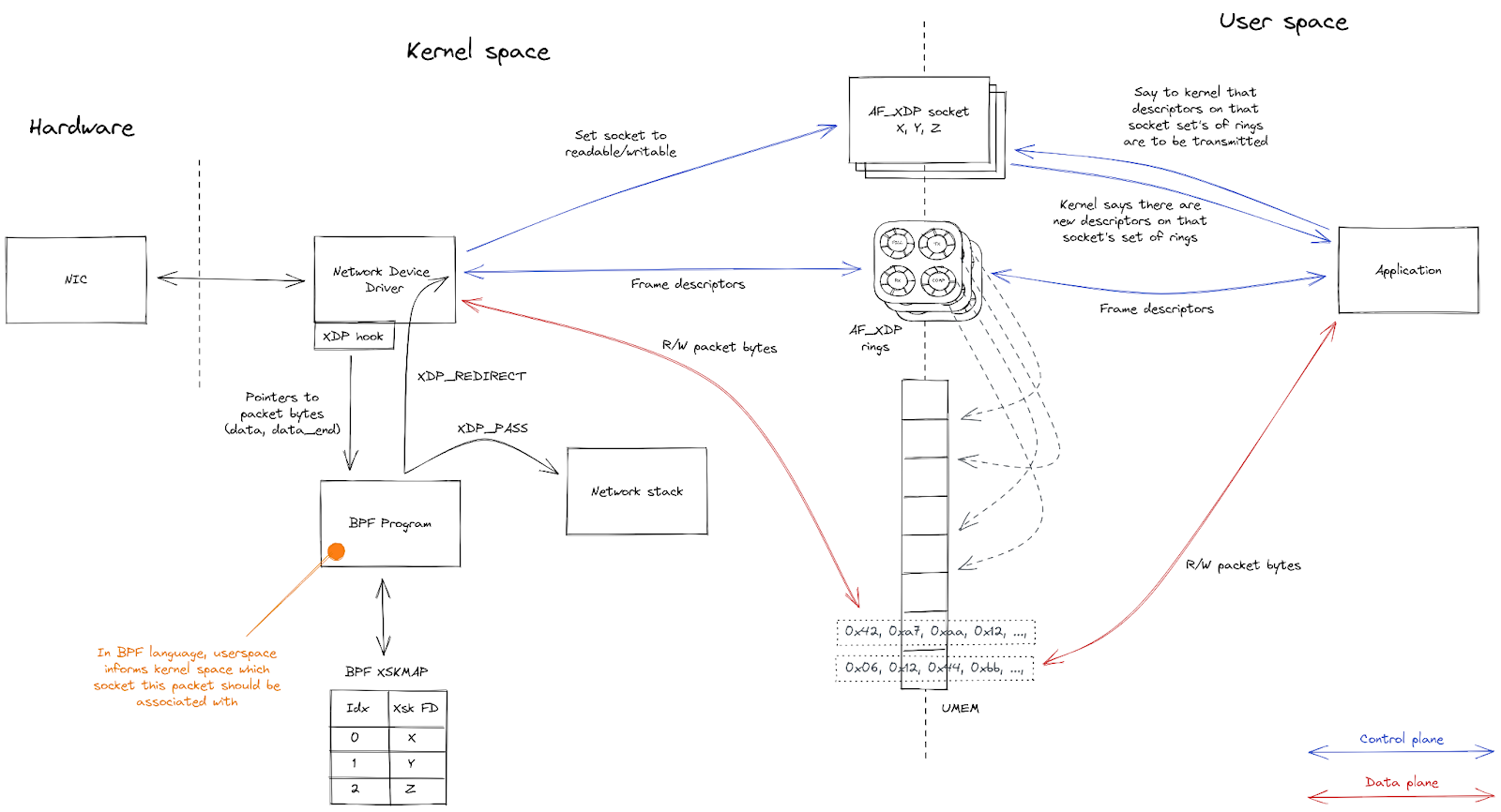
AF_XDP is the high performance asynchronous user-space networking API in the Linux kernel. For network devices that support it, AF_XDP provides a way to perform extremely fast, zero-copy packet forwarding using a memory buffer that’s shared between the kernel and a user-space application.
A number of components need to be set up by the user-space application to start interacting with the packets entering a network device using AF_XDP.
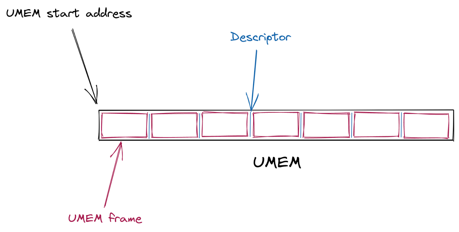
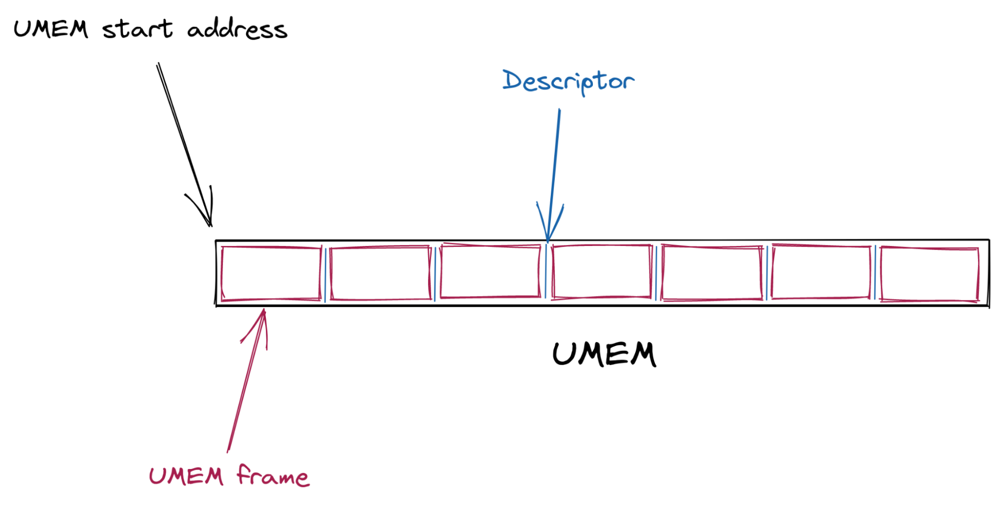
First, a shared packet buffer (UMEM) is created. This UMEM is divided into equal-sized “frames” that are referenced by a “descriptor address,” which is just the offset from the start of the UMEM.
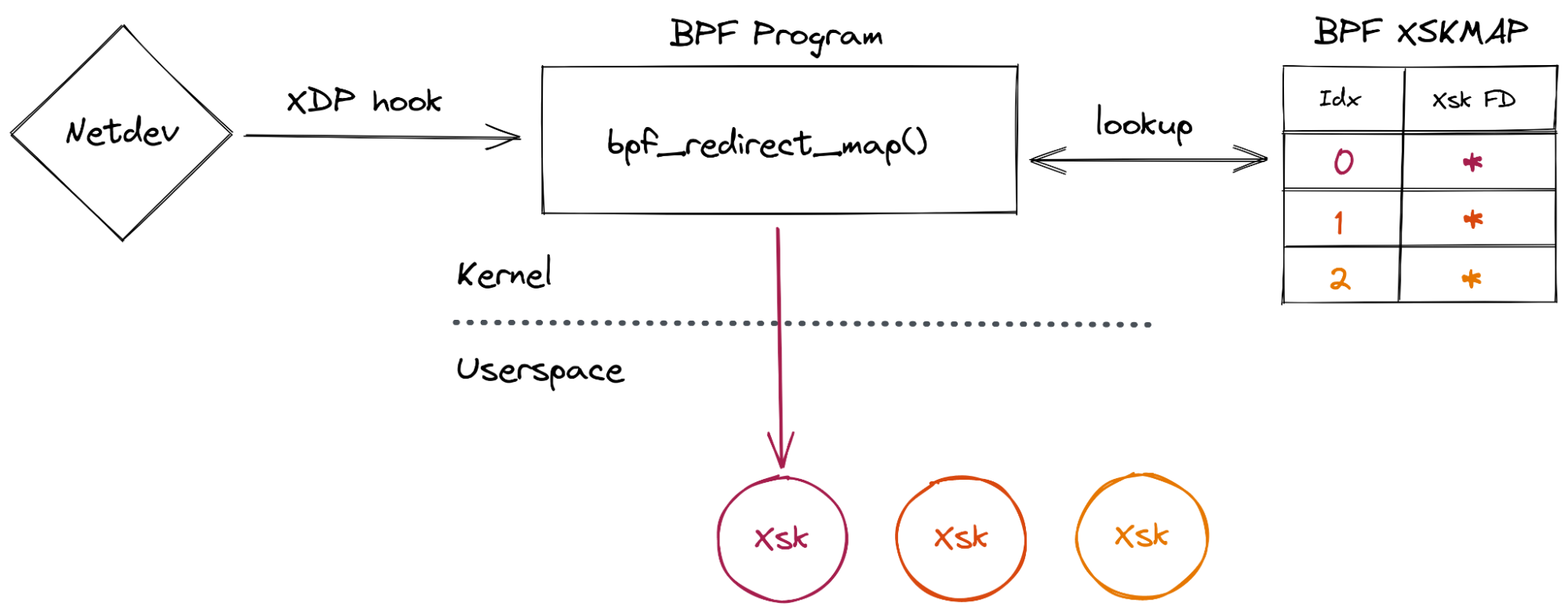
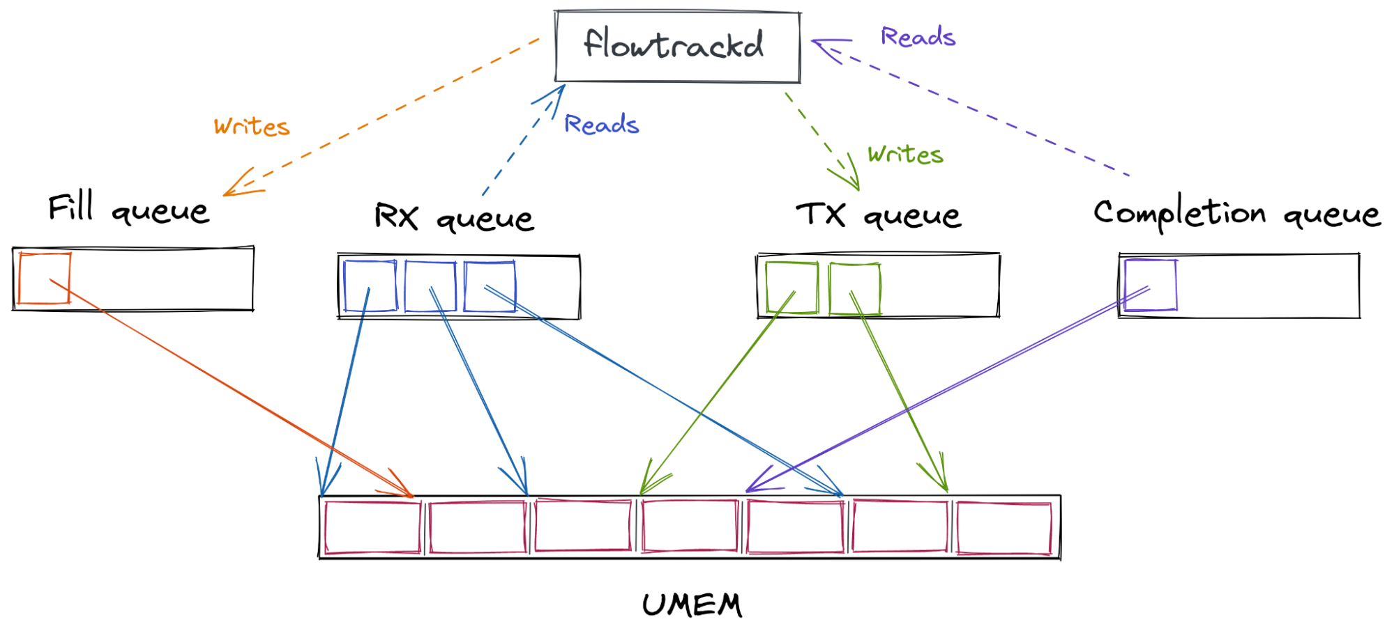
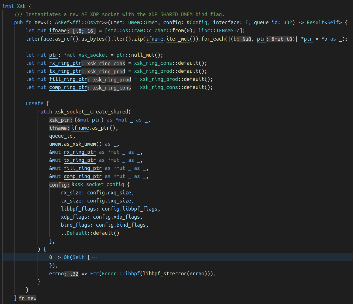
Next, multiple AF_XDP sockets (XSKs) are created – one for each hardware queue on the network device – and bound to the UMEM. Each of these sockets provides four ring buffers (or “queues”) which are used to send descriptors back and forth between the kernel and user-space.
User-space sends packets by taking an unused descriptor and copying the packet into that descriptor (or rather, into the UMEM frame that the descriptor points to). It gives the descriptor to the kernel by enqueueing it on the TX queue. Some time later, the kernel dequeues the descriptor from the TX queue and transmits the packet that it points to out of the network device. Finally, the kernel gives the descriptor back to user-space by enqueueing it on the COMPLETION queue, so that user-space can reuse it later to send another packet.
To receive packets, user-space provides the kernel with unused descriptors by enqueueing them on the FILL queue. The kernel copies packets it receives into these unused descriptors, and then gives them to user-space by enqueueing them on the RX queue. Once user-space processes the packets it dequeues from the RX queue, it either transmits them back out of the network device by enqueueing them on the TX queue, or it gives them back to the kernel for later reuse by enqueueing them on the FILL queue.
Queue
User space
Kernel space
Content description
COMPLETION
Consumes
Produces
Descriptors containing a packet that was successfully transmitted by the kernel
FILL
Produces
Consumes
Descriptors that are empty and ready to be used by the kernel to receive packets
RX
Consumes
Produces
Descriptors containing a packet that was recently received by the kernel
TX
Produces
Consumes
Descriptors containing a packet that is ready to be transmitted by the kernel
Finally, a BPF program is attached to the network device. Its job is to direct incoming packets to whichever XSK is associated with the specific hardware queue that the packet was received on.
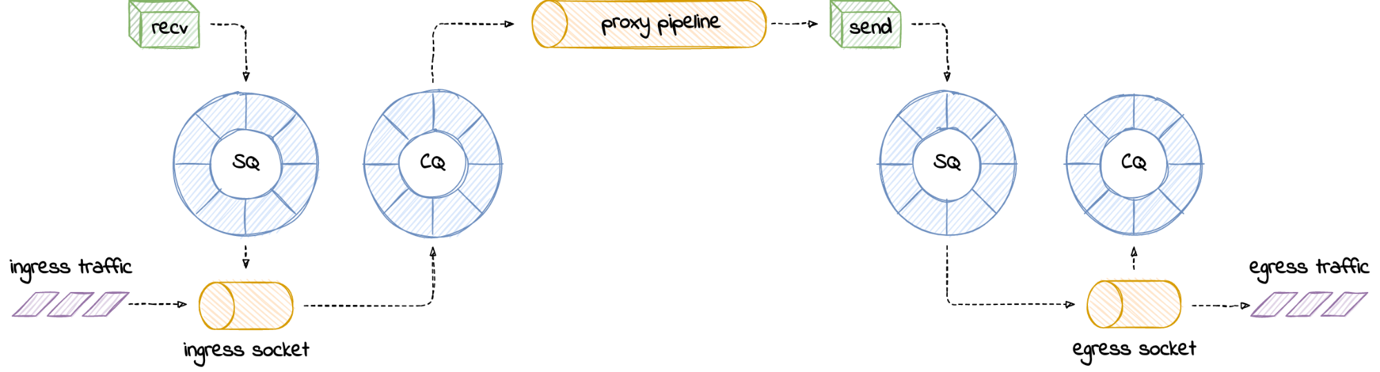
Here is an overview of the interactions between the kernel and user-space:
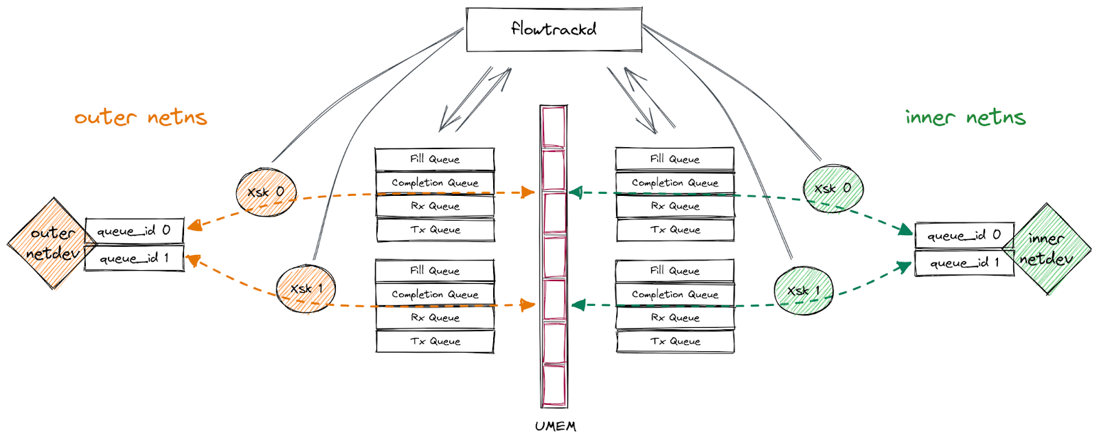
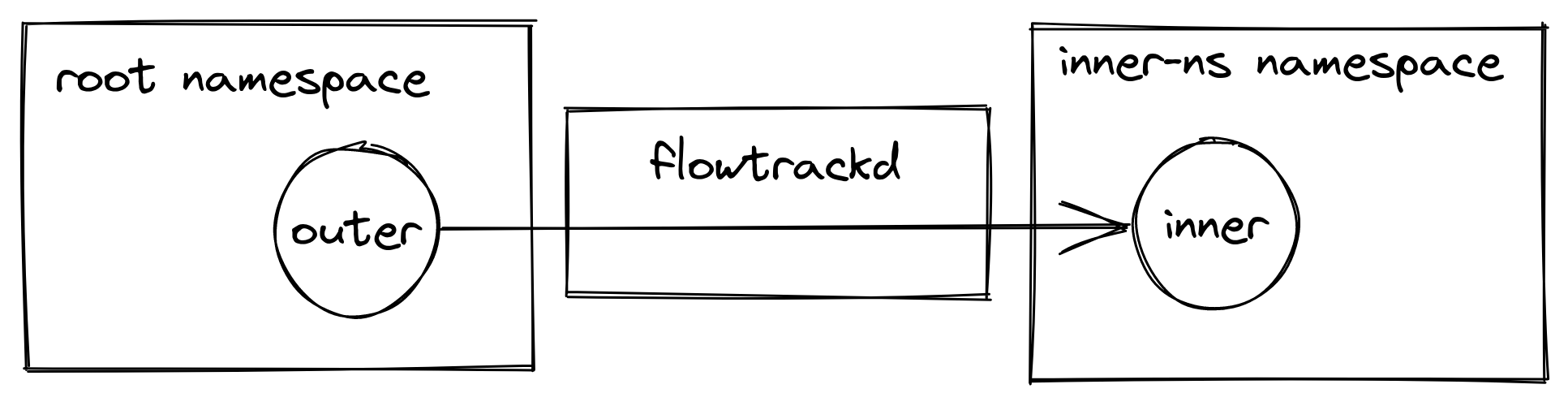
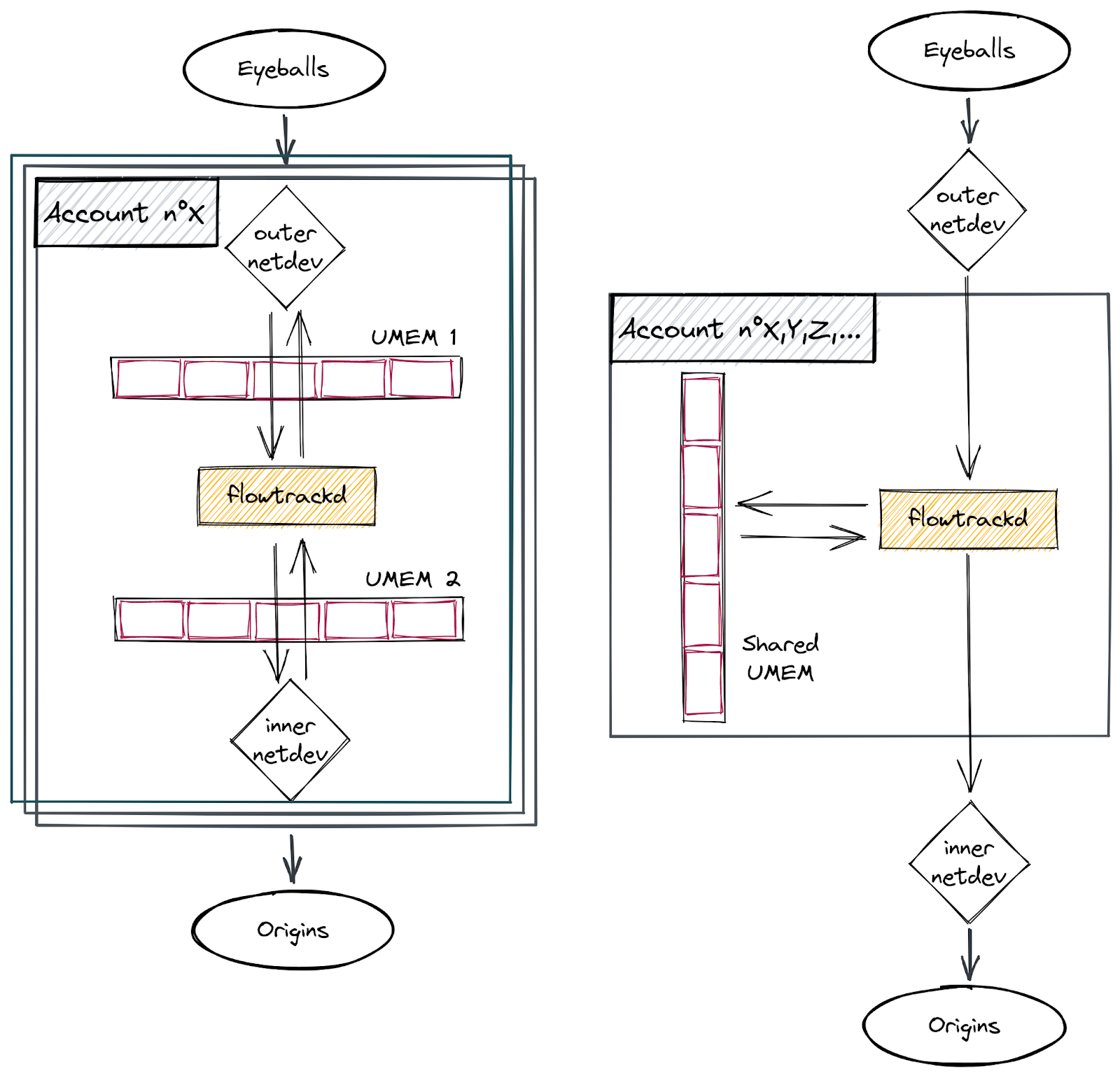
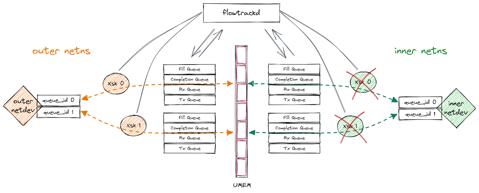
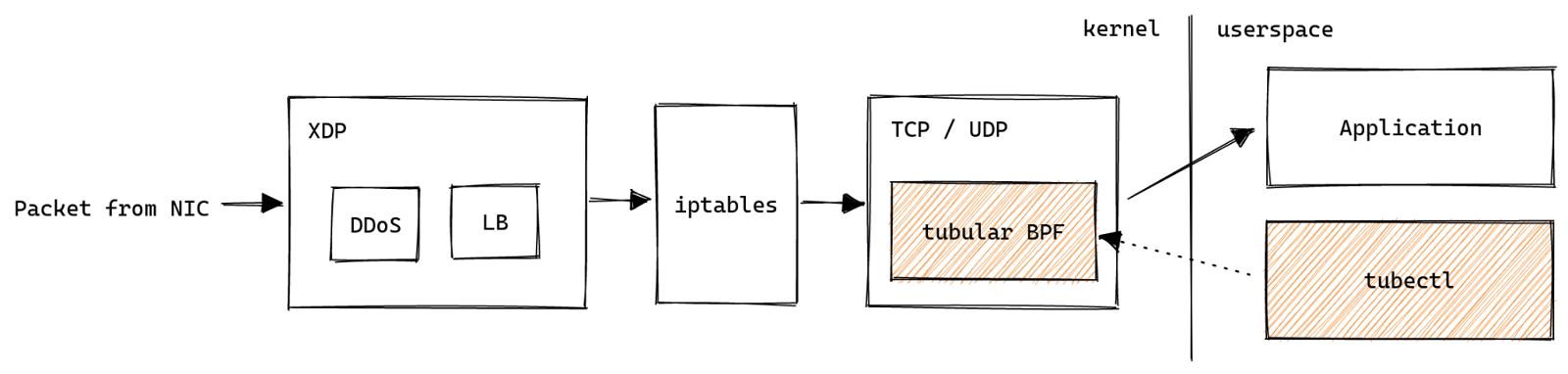
Our setup
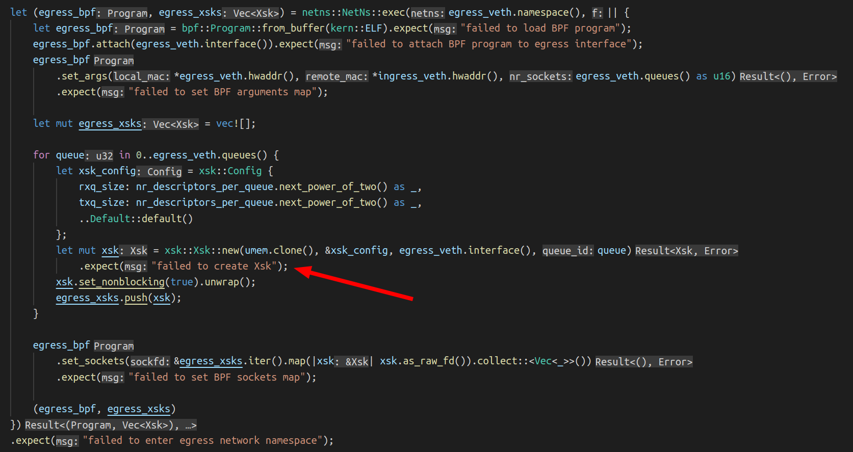
Our application uses AF_XDP on a pair of multi-queue veth interfaces (“outer” and “inner”) that are each in different network namespaces. We follow the process outlined above to bind an XSK to each of the interfaces’ queues, forward packets from one interface to the other, send packets back out of the interface they were received on, or drop them. This functionality enables us to implement bidirectional traffic inspection to perform DDoS mitigation logic.
This setup is depicted in the following diagram:
Information gathering
All we knew to start with was that our program was occasionally seeing corruption that seemed to be impossible. We didn’t know what these corrupt packets actually looked like. It was possible that their contents would reveal more details about the bug and how to reproduce it, so our first step was to log the packet bytes and discard the packet instead of panicking. We could then take the logs with packet bytes in them and create a PCAP file to analyze with Wireshark. This showed us that the packets looked mostly normal, except for Wireshark’s TCP analyzer complaining that their “IPv4 total length exceeds packet length”. In other words, the “total length” IPv4 header field said the packet should be (for example) 60 bytes long, but the packet itself was only 56 bytes long.
Lengths mismatch
Could it be possible that the number of bytes we read from the RX ring was incorrect? Let’s check.
This context structure contains two pointers (as __u32) referring to start and the end of the packet. Getting the packet length can be done by subtracting data from data_end.
If we compare that value with the one we get from the descriptors, we would surely find they are the same right?
We can use the BPF helper function bpf_xdp_adjust_meta() (since the veth driver supports it) to declare a metadata space that will hold the packet buffer length that we computed. We use it the same way this kernel sample code does.
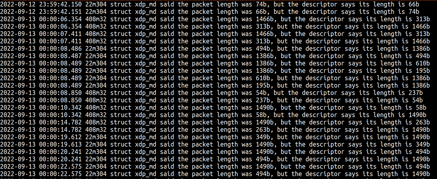
After deploying the new code in production, we saw the following lines in our logs:
Here you can see three interesting things:
As we theorized, the length of the packet when first seen in XDP doesn’t match the length present in the descriptor.
We had already observed from our truncated packet panics that sometimes the descriptor length is shorter than the actual packet length, however the prints show that sometimes the descriptor length might be larger than the real packet bytes.
These often appeared to happen in “pairs” where the XDP length and descriptor length would swap between packets.
Two packets and one buffer?
Seeing the XDP and descriptor lengths swap in “pairs” was perhaps the first lightbulb moment. Are these two different packets being written to the same buffer? This also revealed a key piece of information that we failed to add to our debug prints, the descriptor address! We took this opportunity to print additional information like the packet bytes, and to print at multiple locations in the path to see if anything changed over time.
The real key piece of information that these debug prints revealed was that not only were each swapped “pair” sharing a descriptor address, but nearly every corrupt packet on a single server was always using the same descriptor address. Here you can see 49750 corrupt packets that all used descriptor address 69837056:
This was the second lightbulb moment. Not only are we trying to copy two packets to the same buffer, but it is always the same buffer. Perhaps the problem is that this descriptor has been inserted into the AF_XDP rings twice? We tested this theory by updating our consumer code to test if a batch of descriptors read from the RX ring ever contained the same descriptor twice. This wouldn’t guarantee that the descriptor isn’t in the ring twice since there is no guarantee that the two descriptors will be in the same read batch, but we were lucky enough that it did catch the same descriptor twice in a single read proving this was our issue. In hindsight the linux kernel AF_XDP documentation points out this very issue:
Q: My packets are sometimes corrupted. What is wrong?
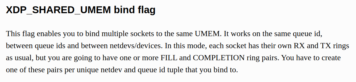
A: Care has to be taken not to feed the same buffer in the UMEM into more than one ring at the same time. If you for example feed the same buffer into the FILL ring and the TX ring at the same time, the NIC might receive data into the buffer at the same time it is sending it. This will cause some packets to become corrupted. Same thing goes for feeding the same buffer into the FILL rings belonging to different queue ids or netdevs bound with the XDP_SHARED_UMEM flag.
We now understand why we have corrupt packets, but we still don’t understand how a descriptor ever ends up in the AF_XDP rings twice. I would love to blame this on a kernel bug, but as the documentation points out this is more likely that we’ve placed the descriptor in the ring twice in our application. Additionally, since this is listed as a FAQ for AF_XDP we will need sufficient evidence proving that this is caused by a kernel bug and not user error before reporting to the kernel mailing list(s).
Tracking descriptor transitions
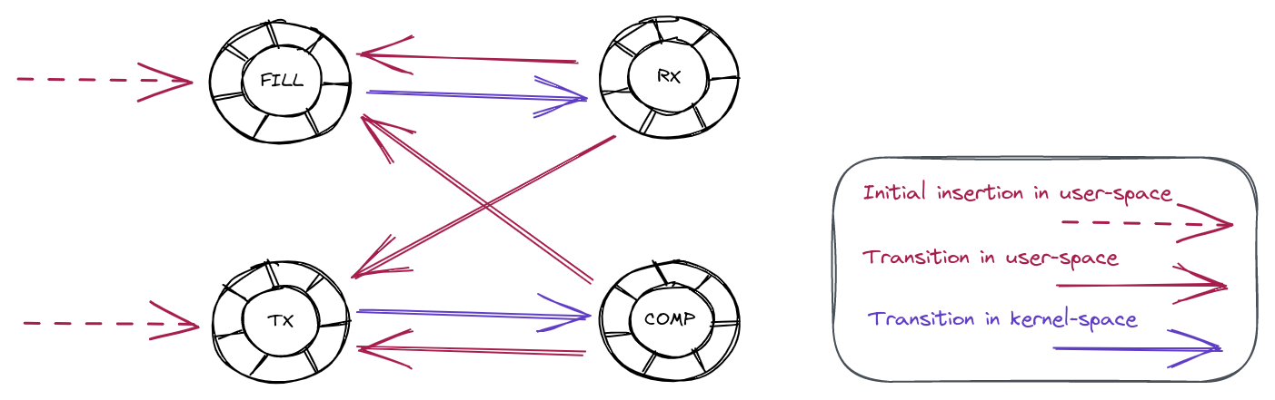
Auditing our application code did not show any obvious location where we might be inserting the same descriptor address into either the FILL or TX ring twice. We do however know that descriptors transition through a set of known states, and we could track those transitions with a state machine. The below diagram shows all the possible valid transitions:
For example, a descriptor going from the RX ring to either the FILL or the TX ring is a perfectly valid transition. On the other hand, a descriptor going from the FILL ring to the COMP ring is an invalid transition.
To test the validity of the descriptor transitions, we added code to track their membership across the rings. This produced some of the following log messages:
Nov 16 23:49:01 fuzzer4 flowtrackd[45807]: thread 'flowtrackd-ZrBh' panicked at 'descriptor 26476800 transitioned from Fill to Tx'
Nov 17 02:09:01 fuzzer4 flowtrackd[45926]: thread 'flowtrackd-Ay0i' panicked at 'descriptor 18422016 transitioned from Comp to Rx'
Nov 29 10:52:08 fuzzer4 flowtrackd[83849]: thread 'flowtrackd-5UYF' panicked at 'descriptor 3154176 transitioned from Tx to Rx'
The first print shows a descriptor was put on the FILL ring and transitioned directly to the TX ring without being read from the RX ring first. This appears to hint at a bug in our application, perhaps indicating that our application duplicates the descriptor putting one copy in the FILL ring and the other copy in the TX ring.
The second invalid transition happened for a descriptor moving from the COMP ring to the RX ring without being put first on the FILL ring. This appears to hint at a kernel bug, perhaps indicating that the kernel duplicated a descriptor and put it both in the COMP ring and the RX ring.
The third invalid transition was from the TX to the RX ring without going through the FILL or COMP ring first. This seems like an extended case of the previous COMP to RX transition and again hints at a possible kernel bug.
Confused by the results we double-checked our tracking code and attempted to find any possible way our application could duplicate a descriptor putting it both in the FILL and TX rings. With no bugs found we felt we needed to gather more information.
Using ftrace as a “flight recorder”
While using a state machine to catch invalid descriptor transitions was able to catch these cases, it still lacked a number of important details which might help track down the ultimate cause of the bug. We still didn’t know if the bug was a kernel issue or an application issue. Confusingly the transition states seemed to indicate it was both.
To gather some more information we ideally wanted to be able to track the history of a descriptor. Since we were using a shared UMEM a descriptor could in theory transition between interfaces, and receive queues. Additionally, our application uses a single green thread to handle each XSK, so it might be interesting to track those descriptor transitions by XSK, CPU, and thread. A simple but unscalable way to achieve this would be to simply print this information at every transition point. This of course is not really an option for a production environment that needs to be able to process millions of packets per second. Both the amount of data produced and the overhead of printing that information will not work.
Up to this point we had been carefully debugging this issue in production systems. The issue was rare enough that even with our large production deployment it might take a day for some production machines to start to display the issue. If we did want to explore more resource intensive debugging techniques we needed to see if we could reproduce this in a test environment. For this we created 10 virtual machines that were continuously load testing our application with iperf. Fortunately with this setup we were able to reproduce the issue about once a day, giving us some more freedom to try some more resource intensive debugging techniques.
Even using a virtual machine it still doesn’t scale to print logs at every descriptor transition, but do you really need to see every transition? In theory the most interesting events are the events right before the bug occurs. We could build something that internally keeps a log of the last N events and only dump that log when the bug occurs. Something like a black box flight recorder used in airplanes to track the events leading up to a crash. Fortunately for us, we don’t really need to build this, and instead can use the Linux kernel’s ftrace feature, which has some additional features that might help us ultimately track down the cause of this bug.
ftrace is a kernel feature that operates by internally keeping a set of per-CPU ring buffers of trace events. Each event stored in the ring buffer is time-stamped and contains some additional information about the context where the event occurred, the CPU, and what process or thread was running at the time of the event. Since these events are stored in per-CPU ring buffers, once the ring is full, new events will overwrite the oldest events leaving a log of the most recent events on that CPU. Effectively we have our flight recorder that we desired, all we need to do is add our events to the ftrace ring buffers and disable tracing when the bug occurs.
ftrace is controlled using virtual files in the debugfs filesystem. Tracing can be enabled and disabled by writing either a 1 or a 0 to:
/sys/kernel/debug/tracing/tracing_on
We can update our application to insert our own events into the tracing ring buffer by writing our messages into the trace_marker file:
/sys/kernel/debug/tracing/trace_marker
And finally after we’ve reproduced the bug and our application has disabled tracing we can extract the contents of all the ring buffers into a single trace file by reading the trace file:
/sys/kernel/debug/tracing/trace
It is worth noting that writing messages to the trace_marker virtual file still involves making a system call and copying your message into the ring buffers. This can still add overhead and in our case where we are logging several prints per packet that overhead might be significant. Additionally, ftrace is a systemwide kernel tracing feature, so you may need to either adjust the permissions of virtual files, or run your application with the appropriate permissions.
There is of course one more big advantage of using ftrace to assist in debugging this issue. As shown above we can log or own application messages to ftrace using the trace_marker file, but at its core ftrace is a kernel tracing feature. This means that we can additionally use ftrace to log events from the kernel side of the AF_XDP packet processing. There are several ways to do this, but for our purposes we used kprobes so that we could target very specific lines of code and print some variables. kprobes can be created directly in ftrace, but I find it easier to create them using the “perf probe” command of perf tool in Linux. Using the “-L” and “-V” arguments you can find which lines of a function can be probed and which variables can be viewed at those probe points. Finally, you can add the probe with the “-a” argument. For example after examining the kernel code we insert the following probe in the receive path of a XSK:
perf probe -a '__xsk_rcv_zc:7 addr len xs xs->pool->fq xs->dev'
This will probe line 7 of __xsk_rcv_zc() and print the descriptor address, the packet length, the XSK address, the fill queue address and the net device address. For context here is what __xsk_rcv_zc() looks like from the perf probe command:
In our case line 7 is the call to xskq_prod_reserve_desc(). At this point in the code the kernel has already removed a descriptor from the FILL queue and copied a packet into that descriptor. The call to xsk_prod_reserve_desc() will ensure that there is space in the RX queue, and if there is space will add that descriptor to the RX queue. It is important to note that while xskq_prod_reserve_desc() will put the descriptor in the RX queue it does not update the producer pointer of the RX ring or notify the XSK that packets are ready to be read because the kernel tries to batch these operations.
Similarly, we wanted to place a probe in the transmit path on the kernel side and ultimately placed the following probe:
perf probe -a 'xp_raw_get_data:0 addr'
There isn’t much interesting to show here in the code, but this probe is placed at a location where descriptors have been removed from the TX queue but have not yet been put in the COMPLETION queue.
In both of these probes it would have been nice to put the probes at the earliest location where descriptors were added or removed from the XSK queues, and to print as much information as possible at these locations. However, in practice the locations where kprobes can be placed and the variables available at those locations limits what can be seen.
With the probes created we still need to enable them to be seen in ftrace. This can be done with:
With our application updated to trace the transition of every descriptor and stop tracing when an invalid transition occurred we were ready to test again.
Tracking descriptor state is not enough
Unfortunately our initial test of our “flight recorder” didn’t immediately tell us anything new. Instead, it mostly confirmed what we already knew, which was that somehow we would end up in a state with the same descriptor twice. It also highlighted the fact that catching an invalid descriptor transition doesn’t mean you have caught the earliest point where the duplicate descriptor appeared. For example assume we have our descriptor A and our duplicate A’. If these are already both present in the FILL queue it is perfectly valid to:
RX A -> FILL A RX A’ -> FILL A’
This can occur for many cycles, before an invalid transition eventually occurs when both descriptors are seen either in the same batch or between queues.
Instead, we needed to rethink our approach. We knew that the kernel removes descriptors from the FILL queue, fills them, and places them in the RX queue. This means that for any given XSK the order that descriptors are inserted into the FILL queue should match the order that they come out of the RX queue. If a descriptor was ever duplicated in this kernel RX path we should see the duplicate descriptor appear out-of-order. With this in mind we updated our application to independently track the order of the FILL queue using a double ended queue. As our application puts descriptors into the FILL queue we also push the descriptor address into the tail of our tracking queue and when we receive packets we pop the descriptor address from the head of our tracking queue and ensure the address matches. If it ever doesn’t match we again can log to trace_marker and stop ftrace.
Below is the end of the first trace we captured with the updated code tracking the order of the FILL to RX queues. The color has been added to improve readability:
Here you can see the power of our ftrace flight recorder. For example, we can follow the full cycle of descriptor 0x16ce900 as it is first received in the kernel, received by our application which forwards the packet by adding to the TX queue, the kernel transmitting, and finally our application receiving the completion and placing the descriptor back in the FILL queue.
The trace starts to get interesting on the next two packets received by the kernel. We can see 0x160a100 received first in the kernel and then by our application. However things go wrong when the kernel receives 0x13d3900 but our application receives 0x1229100. The last print of the trace shows the result of our descriptor order tracking. We can see that the kernel side appears to match our next expected descriptor and the next two descriptors, yet unexpectedly we see 0x1229100 arrive out of nowhere. We do think that the descriptor is present in the FILL queue, but it is much further down the line in the queue. Another potentially interesting detail is that between 0x160a100 and 0x13d3900 the kernel’s softirq switches from CPU 1 to CPU 2.
If you recall, our __xsk_rcv_zc_L7 kprobe was placed on the call to xskq_prod_reserve_desc() which adds the descriptor to the RX queue. Below we can examine that function to see if there are any clues on how the descriptor address received by our application could be different from what we think should have been inserted by the kernel.
Here you can see that the queue’s cached_prod pointer is incremented first before we update the descriptor address and length. As the name implies the cached_prod pointer isn’t the actual producer pointer which means that at some point xsk_flush() must be called to sync the cached_prod pointer and the prod pointer to actually expose the newly received descriptors to user-mode. Perhaps there is a race where xsk_flush() is called after updating the cached_prod pointer, but before the actual descriptor address has been updated in the ring? If this were to occur our application would see the old descriptor address from that slot in the RX queue and would cause us to “duplicate” that descriptor.
We can test our theory by making two more changes. First we can update our application to write back a known “poisoned” descriptor address to each RX queue slot after we have received a packet. In this case we chose 0xdeadbeefdeadbeef as our known invalid address and if we ever receive this value back out of the RX queue we know a race has occurred and exposed an uninitialized descriptor. The second change we can make is to add a kprobe on xsk_flush() to see if we can actually capture the race in the trace.
Here we appear to have our smoking gun. As we predicted we can see that xsk_flush() is called on CPU 0 while a softirq is currently in progress on CPU 2. After the flush our application sees the expected 0xff0900 filled in from the softirq on CPU 0, and then 0xdeadbeefdeadbeef which is our poisoned uninitialized descriptor address.
We now have evidence that the following order of operations is happening:
CPU 2                                                   CPU 0
-----------------------------------                     --------------------------------
__xsk_rcv_zc(struct xdp_sock *xs):                      xsk_flush(struct xdp_sock *xs):

idx = xs->rx->cached_prod++ & xs->rx->ring_mask;
                                                        // Flush the cached pointer as the new head pointer of
                                                        // the RX ring.
                                                        smp_store_release(&xs->rx->ring->producer, xs->rx->cached_prod);

                                                        // Notify user-side that new descriptors have been produced to
                                                        // the RX ring.
                                                        sock_def_readable(&xs->sk);

                                                        // flowtrackd reads a descriptor "too soon" where the addr
                                                        // and/or len fields have not yet been updated.
xs->rx->ring->desc[idx].addr = addr;
xs->rx->ring->desc[idx].len = len;
The AF_XDP documentation states that: “All rings are single-producer/single-consumer, so the user-space application needs explicit synchronization of multiple processes/threads are reading/writing to them.” The explicit synchronization requirement must also apply on the kernel side. How can two operations on the RX ring of a socket run at the same time?
On Linux, a mechanism called NAPI prevents CPU interrupts from occurring every time a packet is received by the network interface. It instructs the network driver to process a certain amount of packets at a frequent interval. For the veth driver that polling function is called veth_poll, and it is registered as the function handler for each queue of the XDP enabled network device. A NAPI-compliant network driver provides the guarantee that the processing of the packets tied to a NAPI context (struct napi_struct *napi) will not be happening at the same time on multiple processors. In our case, a NAPI context exists for each queue of the device which means per AF_XDP socket and their associated set of ring buffers (RX, TX, FILL, COMPLETION).
static int veth_poll(struct napi_struct *napi, int budget)
{
	struct veth_rq *rq =
		container_of(napi, struct veth_rq, xdp_napi);
	struct veth_stats stats = {};
	struct veth_xdp_tx_bq bq;
	int done;

	bq.count = 0;

	xdp_set_return_frame_no_direct();
	done = veth_xdp_rcv(rq, budget, &bq, &stats);

	if (done < budget && napi_complete_done(napi, done)) {
		/* Write rx_notify_masked before reading ptr_ring */
		smp_store_mb(rq->rx_notify_masked, false);
		if (unlikely(!__ptr_ring_empty(&rq->xdp_ring))) {
			if (napi_schedule_prep(&rq->xdp_napi)) {
				WRITE_ONCE(rq->rx_notify_masked, true);
				__napi_schedule(&rq->xdp_napi);
			}
		}
	}

	if (stats.xdp_tx > 0)
		veth_xdp_flush(rq, &bq);
	if (stats.xdp_redirect > 0)
		xdp_do_flush();
	xdp_clear_return_frame_no_direct();

	return done;
}
veth_xdp_rcv() processes as many packets as the budget variable is set to, marks the NAPI processing as complete, potentially reschedules a NAPI polling, and then, calls xdp_do_flush(), breaking the NAPI guarantee cited above. After the call to napi_complete_done(), any CPU is free to execute the veth_poll() function before all the flush operations of the previous call are complete, allowing the race on the RX ring.
The race condition can be fixed by completing all the packet processing before signaling the NAPI poll as complete. The patch as well as the discussion on the kernel mailing list that lead to the fix are available here: [PATCH] veth: Fix race with AF_XDP exposing old or uninitialized descriptors. The patch was recently merged upstream.
Conclusion
We’ve found and fixed a race condition in the Linux virtual ethernet (veth) driver that was corrupting packets for AF_XDP enabled devices!
This issue was a tough one to find (and to reproduce) but logical iterations lead us all the way down to the internals of the Linux kernel where we saw that a few lines of code were not executed in the correct order.
A rigorous methodology and the knowledge of the right debugging tools are essential to go about tracking down the root cause of potentially complex bugs.
This was important for us to fix because while TCP was designed to recover from occasional packet drops, randomly dropping legitimate packets slightly increased the latency of connection establishments and data transfers across our network.
Interested about other deep dive kernel debugging journeys? Read more of them on our blog!
We want our digital data to be safe. We want to visit websites, send bank details, type passwords, sign documents online, login into remote computers, encrypt data before storing it in databases and be sure that nobody can tamper with it. Cryptography can provide a high degree of data security, but we need to protect cryptographic keys.
At the same time, we can’t have our key written somewhere securely and just access it occasionally. Quite the opposite, it’s involved in every request where we do crypto-operations. If a site supports TLS, then the private key is used to establish each connection.
Unfortunately cryptographic keys sometimes leak and when it happens, it is a big problem. Many leaks happen because of software bugs and security vulnerabilities. In this post we will learn how the Linux kernel can help protect cryptographic keys from a whole class of potential security vulnerabilities: memory access violations.
Memory access violations
According to the NSA, around 70% of vulnerabilities in both Microsoft’s and Google’s code were related to memory safety issues. One of the consequences of incorrect memory accesses is leaking security data (including cryptographic keys). Cryptographic keys are just some (mostly random) data stored in memory, so they may be subject to memory leaks like any other in-memory data. The below example shows how a cryptographic key may accidentally leak via stack memory reuse:
broken.c
#include <stdio.h>
#include <stdint.h>

static void encrypt(void)
{
    uint8_t key[] = "hunter2";
    printf("encrypting with super secret key: %s\n", key);
}

static void log_completion(void)
{
    /* oh no, we forgot to init the msg */
    char msg[8];
    printf("not important, just fyi: %s\n", msg);
}

int main(void)
{
    encrypt();
    /* notify that we're done */
    log_completion();
    return 0;
}
Compile and run our program:
$ gcc -o broken broken.c
$ ./broken
encrypting with super secret key: hunter2
not important, just fyi: hunter2
Oops, we printed the secret key in the “fyi” logger instead of the intended log message! There are two problems with the code above:
we didn’t securely destroy the key in our pseudo-encryption function (by overwriting the key data with zeroes, for example), when we finished using it
our buggy logging function has access to any memory within our process
And while we can probably easily fix the first problem with some additional code, the second problem is the inherent result of how software runs inside the operating system.
Each process is given a block of contiguous virtual memory by the operating system. It allows the kernel to share limited computer resources among several simultaneously running processes. This approach is called virtual memory management. Inside the virtual memory a process has its own address space and doesn’t have access to the memory of other processes, but it can access any memory within its address space. In our example we are interested in a piece of process memory called the stack.
The stack consists of stack frames. A stack frame is dynamically allocated space for the currently running function. It contains the function’s local variables, arguments and return address. When compiling a function the compiler calculates how much memory needs to be allocated and requests a stack frame of this size. Once a function finishes execution the stack frame is marked as free and can be used again. A stack frame is a logical block, it doesn’t provide any boundary checks, it’s not erased, just marked as free. Additionally, the virtual memory is a contiguous block of addresses. Both of these statements give the possibility for malware/buggy code to access data from anywhere within virtual memory.
The stack of our program broken.c will look like:
At the beginning we have a stack frame of the main function. Further, the main() function calls encrypt() which will be placed on the stack immediately below the main() (the code stack grows downwards). Inside encrypt() the compiler requests 8 bytes for the key variable (7 bytes of data + C-null character). When encrypt() finishes execution, the same memory addresses are taken by log_completion(). Inside the log_completion() the compiler allocates eight bytes for the msg variable. Accidentally, it was put on the stack at the same place where our private key was stored before. The memory for msg was only allocated, but not initialized, the data from the previous function left as is.
Additionally, to the code bugs, programming languages provide unsafe functions known for the safe-memory vulnerabilities. For example, for C such functions are printf(), strcpy(), gets(). The function printf() doesn’t check how many arguments must be passed to replace all placeholders in the format string. The function arguments are placed on the stack above the function stack frame, printf() fetches arguments according to the numbers and type of placeholders, easily going off its arguments and accessing data from the stack frame of the previous function.
The NSA advises us to use safety-memory languages like Python, Go, Rust. But will it completely protect us?
The Python compiler will definitely check boundaries in many cases for you and notify with an error:
>>> print("x: {}, y: {}, {}".format(1, 2))
Traceback (most recent call last):
  File "<stdin>", line 1, in <module>
IndexError: Replacement index 2 out of range for positional args tuple
However, this is a quote from one of 36 (for now) vulnerabilities:
Python 2.7.14 is vulnerable to a Heap-Buffer-Overflow as well as a Heap-Use-After-Free.
Golang has its own list of overflow vulnerabilities, and has an unsafe package. The name of the package speaks for itself, usual rules and checks don’t work inside this package.
Heartbleed
In 2014, the Heartbleed bug was discovered. The (at the time) most used cryptography library OpenSSL leaked private keys. We experienced it too.
Mitigation
So memory bugs are a fact of life, and we can’t really fully protect ourselves from them. But, given the fact that cryptographic keys are much more valuable than the other data, can we do better protecting the keys at least?
As we already said, a memory address space is normally associated with a process. And two different processes don’t share memory by default, so are naturally isolated from each other. Therefore, a potential memory bug in one of the processes will not accidentally leak a cryptographic key from another process. The security of ssh-agent builds on this principle. There are always two processes involved: a client/requester and the agent.
The agent will never send a private key over its request channel. Instead, operations that require a private key will be performed by the agent, and the result will be returned to the requester. This way, private keys are not exposed to clients using the agent.
A requester is usually a network-facing process and/or processing untrusted input. Therefore, the requester is much more likely to be susceptible to memory-related vulnerabilities but in this scheme it would never have access to cryptographic keys (because keys reside in a separate process address space) and, thus, can never leak them.
At Cloudflare, we employ the same principle in Keyless SSL. Customer private keys are stored in an isolated environment and protected from Internet-facing connections.
Linux Kernel Key Retention Service
The client/requester and agent approach provides better protection for secrets or cryptographic keys, but it brings some drawbacks:
we need to develop and maintain two different programs instead of one
we also need to design a well-defined-interface for communication between the two processes
we need to implement the communication support between two processes (Unix sockets, shared memory, etc.)
we might need to authenticate and support ACLs between the processes, as we don’t want any requester on our system to be able to use our cryptographic keys stored inside the agent
we need to ensure the agent process is up and running, when working with the client/requester process
What if we replace the agent process with the Linux kernel itself?
it is already running on our system (otherwise our software would not work)
it has a well-defined interface for communication (system calls)
Initially it was designed for kernel services like dm-crypt/ecryptfs, but later was opened to use by userspace programs. It gives us some advantages:
the keys are stored outside the process address space
the well-defined-interface and the communication layer is implemented via syscalls
the keys are kernel objects and so have associated permissions and ACLs
the keys lifecycle can be implicitly bound to the process lifecycle
The Linux Kernel Key Retention Service operates with two types of entities: keys and keyrings, where a keyring is a key of a special type. If we put it into analogy with files and directories, we can say a key is a file and a keyring is a directory. Moreover, they represent a key hierarchy similar to a filesystem tree hierarchy: keyrings reference keys and other keyrings, but only keys can hold the actual cryptographic material similar to files holding the actual data.
Keys have types. The type of key determines which operations can be performed over the keys. For example, keys of user and logon types can hold arbitrary blobs of data, but logon keys can never be read back into userspace, they are exclusively used by the in-kernel services.
For the purposes of using the kernel instead of an agent process the most interesting type of keys is the asymmetric type. It can hold a private key inside the kernel and provides the ability for the allowed applications to either decrypt or sign some data with the key. Currently, only RSA keys are supported, but work is underway to add ECDSA key support.
While keys are responsible for safeguarding the cryptographic material inside the kernel, keyrings determine key lifetime and shared access. In its simplest form, when a particular keyring is destroyed, all the keys that are linked only to that keyring are securely destroyed as well. We can create custom keyrings manually, but probably one the most powerful features of the service are the “special keyrings”.
These keyrings are created implicitly by the kernel and their lifetime is bound to the lifetime of a different kernel object, like a process or a user. (Currently there are four categories of “implicit” keyrings), but for the purposes of this post we’re interested in two most widely used ones: process keyrings and user keyrings.
User keyring lifetime is bound to the existence of a particular user and this keyring is shared between all the processes of the same UID. Thus, one process, for example, can store a key in a user keyring and another process running as the same user can retrieve/use the key. When the UID is removed from the system, all the keys (and other keyrings) under the associated user keyring will be securely destroyed by the kernel.
Process keyrings are bound to some processes and may be of three types differing in semantics: process, thread and session. A process keyring is bound and private to a particular process. Thus, any code within the process can store/use keys in the keyring, but other processes (even with the same user id or child processes) cannot get access. And when the process dies, the keyring and the associated keys are securely destroyed. Besides the advantage of storing our secrets/keys in an isolated address space, the process keyring gives us the guarantee that the keys will be destroyed regardless of the reason for the process termination: even if our application crashed hard without being given an opportunity to execute any clean up code – our keys will still be securely destroyed by the kernel.
A thread keyring is similar to a process keyring, but it is private and bound to a particular thread. For example, we can build a multithreaded web server, which can serve TLS connections using multiple private keys, and we can be sure that connections/code in one thread can never use a private key, which is associated with another thread (for example, serving a different domain name).
A session keyring makes its keys available to the current process and all its children. It is destroyed when the topmost process terminates and child processes can store/access keys, while the topmost process exists. It is mostly useful in shell and interactive environments, when we employ the keyctl tool to access the Linux Kernel Key Retention Service, rather than using the kernel system call interface. In the shell, we generally can’t use the process keyring as every executed command creates a new process. Thus, if we add a key to the process keyring from the command line – that key will be immediately destroyed, because the “adding” process terminates, when the command finishes executing. Let’s actually confirm this with bpftrace.
In one terminal we will trace the user_destroy function, which is responsible for deleting a user key:
And in another terminal let’s try to add a key to the process keyring:
$ keyctl add user mykey hunter2 @p
742524855
Going back to the first terminal we can immediately see:
…
Attaching 1 probe...
destroying key 742524855
And we can confirm the key is not available by trying to access it:
$ keyctl print 742524855
keyctl_read_alloc: Required key not available
So in the above example, the key “mykey” was added to the process keyring of the subshell executing keyctl add user mykey hunter2 @p. But since the subshell process terminated the moment the command was executed, both its process keyring and the added key were destroyed.
Instead, the session keyring allows our interactive commands to add keys to our current shell environment and subsequent commands to consume them. The keys will still be securely destroyed, when our main shell process terminates (likely, when we log out from the system).
So by selecting the appropriate keyring type we can ensure the keys will be securely destroyed, when not needed. Even if the application crashes! This is a very brief introduction, but it will allow you to play with our examples, for the whole context, please, reach the official documentation.
Replacing the ssh-agent with the Linux Kernel Key Retention Service
We gave a long description of how we can replace two isolated processes with the Linux Kernel Retention Service. It’s time to put our words into code. We talked about ssh-agent as well, so it will be a good exercise to replace our private key stored in memory of the agent with an in-kernel one. We picked the most popular SSH implementation OpenSSH as our target.
Some minor changes need to be added to the code to add functionality to retrieve a key from the kernel:
$ autoreconf
$ ./configure --with-libs=-lkeyutils --disable-pkcs11
…
$ make
…
Note that we instruct the build system to additionally link with libkeyutils, which provides convenient wrappers to access the Linux Kernel Key Retention Service. Additionally, we had to disable PKCS11 support as the code has a function with the same name as in `libkeyutils`, so there is a naming conflict. There might be a better fix for this, but it is out of scope for this post.
Now that we have the patched OpenSSH – let’s test it. Firstly, we need to generate a new SSH RSA key that we will use to access the system. Because the Linux kernel only supports private keys in the PKCS8 format, we’ll use it from the start (instead of the default OpenSSH format):
Normally, we would be using `ssh-add` to add this key to our ssh agent. In our case we need to use a replacement script, which would add the key to our current session keyring:
ssh-add-keyring.sh
#/bin/bash -e

in=$1
key_desc=$2
keyring=$3

in_pub=$in.pub
key=$(mktemp)
out="${in}_keyring"

function finish {
    rm -rf $key
}
trap finish EXIT

# https://github.com/openssh/openssh-portable/blob/master/PROTOCOL.key
# null-terminanted openssh-key-v1
printf 'openssh-key-v1\0' > $key
# cipher: none
echo '00000004' | xxd -r -p >> $key
echo -n 'none' >> $key
# kdf: none
echo '00000004' | xxd -r -p >> $key
echo -n 'none' >> $key
# no kdf options
echo '00000000' | xxd -r -p >> $key
# one key in the blob
echo '00000001' | xxd -r -p >> $key

# grab the hex public key without the (00000007 || ssh-rsa) preamble
pub_key=$(awk '{ print $2 }' $in_pub | base64 -d | xxd -s 11 -p | tr -d '\n')
# size of the following public key with the (0000000f || ssh-rsa-keyring) preamble
printf '%08x' $(( ${#pub_key} / 2 + 19 )) | xxd -r -p >> $key
# preamble for the public key
# ssh-rsa-keyring in prepended with length of the string
echo '0000000f' | xxd -r -p >> $key
echo -n 'ssh-rsa-keyring' >> $key
# the public key itself
echo $pub_key | xxd -r -p >> $key

# the private key is just a key description in the Linux keyring
# ssh will use it to actually find the corresponding key serial
# grab the comment from the public key
comment=$(awk '{ print $3 }' $in_pub)
# so the total size of the private key is
# two times the same 4 byte int +
# (0000000f || ssh-rsa-keyring) preamble +
# a copy of the public key (without preamble) +
# (size || key_desc) +
# (size || comment )
priv_sz=$(( 8 + 19 + ${#pub_key} / 2 + 4 + ${#key_desc} + 4 + ${#comment} ))
# we need to pad the size to 8 bytes
pad=$(( 8 - $(( priv_sz % 8 )) ))
# so, total private key size
printf '%08x' $(( $priv_sz + $pad )) | xxd -r -p >> $key
# repeated 4-byte int
echo '0102030401020304' | xxd -r -p >> $key
# preamble for the private key
echo '0000000f' | xxd -r -p >> $key
echo -n 'ssh-rsa-keyring' >> $key
# public key
echo $pub_key | xxd -r -p >> $key
# private key description in the keyring
printf '%08x' ${#key_desc} | xxd -r -p >> $key
echo -n $key_desc >> $key
# comment
printf '%08x' ${#comment} | xxd -r -p >> $key
echo -n $comment >> $key
# padding
for (( i = 1; i <= $pad; i++ )); do
    echo 0$i | xxd -r -p >> $key
done

echo '-----BEGIN OPENSSH PRIVATE KEY-----' > $out
base64 $key >> $out
echo '-----END OPENSSH PRIVATE KEY-----' >> $out
chmod 600 $out

# load the PKCS8 private key into the designated keyring
openssl pkcs8 -in $in -topk8 -outform DER -nocrypt | keyctl padd asymmetric $key_desc $keyring
Depending on how our kernel was compiled, we might also need to load some kernel modules for asymmetric private key support:
$ sudo modprobe pkcs8_key_parser
$ ./ssh-add-keyring.sh ~/.ssh/id_rsa myssh @s
Enter pass phrase for ~/.ssh/id_rsa:
723263309
Finally, our private ssh key is added to the current session keyring with the name “myssh”. In addition, the ssh-add-keyring.sh will create a pseudo-private key file in ~/.ssh/id_rsa_keyring, which needs to be passed to the main ssh process. It is a pseudo-private key, because it doesn’t have any sensitive cryptographic material. Instead, it only has the “myssh” identifier in a native OpenSSH format. If we use multiple SSH keys, we have to tell the main ssh process somehow which in-kernel key name should be requested from the system.
Before we start testing it, let’s make sure our SSH server (running locally) will accept the newly generated key as a valid authentication:
$ cat ~/.ssh/id_rsa.pub >> ~/.ssh/authorized_keys
Now we can try to SSH into the system:
$ SSH_AUTH_SOCK="" ./ssh -i ~/.ssh/id_rsa_keyring localhost
The authenticity of host 'localhost (::1)' can't be established.
ED25519 key fingerprint is SHA256:3zk7Z3i9qZZrSdHvBp2aUYtxHACmZNeLLEqsXltynAY.
This key is not known by any other names.
Are you sure you want to continue connecting (yes/no/[fingerprint])? yes
Warning: Permanently added 'localhost' (ED25519) to the list of known hosts.
Linux dev 5.15.79-cloudflare-2022.11.6 #1 SMP Mon Sep 27 00:00:00 UTC 2010 x86_64
…
It worked! Notice that we’re resetting the `SSH_AUTH_SOCK` environment variable to make sure we don’t use any keys from an ssh-agent running on the system. Still the login flow does not request any password for our private key, the key itself is resident of the kernel address space, and we reference it using its serial for signature operations.
User or session keyring?
In the example above, we set up our SSH private key into the session keyring. We can check if it is there:
We might have used user keyring as well. What is the difference? Currently, the “myssh” key lifetime is limited to the current login session. That is, if we log out and login again, the key will be gone, and we would have to run the ssh-add-keyring.sh script again. Similarly, if we log in to a second terminal, we won’t see this key:
Notice that the serial number of the session keyring _ses in the second terminal is different. A new keyring was created and “myssh” key along with the previous session keyring doesn’t exist anymore:
$ SSH_AUTH_SOCK="" ./ssh -i ~/.ssh/id_rsa_keyring localhost
Load key "/home/ignat/.ssh/id_rsa_keyring": key not found
…
If instead we tell ssh-add-keyring.sh to load the private key into the user keyring (replace @s with @u in the command line parameters), it will be available and accessible from both login sessions. In this case, during logout and re-login, the same key will be presented. Although, this has a security downside – any process running as our user id will be able to access and use the key.
Summary
In this post we learned about one of the most common ways that data, including highly valuable cryptographic keys, can leak. We talked about some real examples, which impacted many users around the world, including Cloudflare. Finally, we learned how the Linux Kernel Retention Service can help us to protect our cryptographic keys and secrets.
We also introduced a working patch for OpenSSH to use this cool feature of the Linux kernel, so you can easily try it yourself. There are still many Linux Kernel Key Retention Service features left untold, which might be a topic for another blog post. Stay tuned!
The malware was dubbed “Shikitega” for its extensive use of the popular Shikata Ga Nai polymorphic encoder, which allows the malware to “mutate” its code to avoid detection. Shikitega alters its code each time it runs through one of several decoding loops that AT&T said each deliver multiple attacks, beginning with an ELF file that’s just 370 bytes.
Shikitega also downloads Mettle, a Metasploit interpreter that gives the attacker the ability to control attached webcams and includes a sniffer, multiple reverse shells, process control, shell command execution and additional abilities to control the affected system.
[…]
The final stage also establishes persistence, which Shikitega does by downloading and executing five shell scripts that configure a pair of cron jobs for the current user and a pair for the root user using crontab, which it can also install if not available.
Shikitega also uses cloud hosting solutions to store parts of its payload, which it further uses to obfuscate itself by contacting via IP address instead of domain name. “Without [a] domain name, it’s difficult to provide a complete list of indicators for detections since they are volatile and they will be used for legitimate purposes in a short period of time,” AT&T said.
Bottom line: Shikitega is a nasty piece of code. AT&T recommends Linux endpoint and IoT device managers keep security patches installed, keep EDR software up to date and make regular backups of essential systems.
Over the years I’ve been lurking around the Linux kernel and have investigated the TCP code many times. But when recently we were working on Optimizing TCP for high WAN throughput while preserving low latency, I realized I have gaps in my knowledge about how Linux manages TCP receive buffers and windows. As I dug deeper I found the subject complex and certainly non-obvious.
In this blog post I’ll share my journey deep into the Linux networking stack, trying to understand the memory and window management of the receiving side of a TCP connection. Specifically, looking for answers to seemingly trivial questions:
How much data can be stored in the TCP receive buffer? (it’s not what you think)
How fast can it be filled? (it’s not what you think either!)
Our exploration focuses on the receiving side of the TCP connection. We’ll try to understand how to tune it for the best speed, without wasting precious memory.
A case of a rapid upload
To best illustrate the receive side buffer management we need pretty charts! But to grasp all the numbers, we need a bit of theory.
We’ll draw charts from a receive side of a TCP flow, running a pretty straightforward scenario:
The client opens a TCP connection.
The client does send(), and pushes as much data as possible.
The server doesn’t recv() any data. We expect all the data to stay and wait in the receive queue.
How much data can fit in the server’s receive buffer? It turns out it’s not exactly the same as the default read buffer size on Linux; we’ll get there.
Assuming infinite bandwidth, what is the minimal time – measured in RTT – for the client to fill the receive buffer?
First, there is the buffer budget limit. ss manpage calls it skmem_rb, in the kernel it’s named sk_rcvbuf. This value is most often controlled by the Linux autotune mechanism using the net.ipv4.tcp_rmem setting:
Alternatively it can be manually set with setsockopt(SO_RCVBUF) on a socket. Note that the kernel doubles the value given to this setsockopt. For example SO_RCVBUF=16384 will result in skmem_rb=32768. The max value allowed to this setsockopt is limited to meager 208KiB by default:
The aforementioned blog post discusses why manual buffer size management is problematic – relying on autotuning is generally preferable.
Here’s a diagram showing how skmem_rb budget is being divided:
In any given moment, we can think of the budget as being divided into four parts:
Recv-q: part of the buffer budget occupied by actual application bytes awaiting read().
Another part of is consumed by metadata handling – the cost of struct sk_buff and such.
Those two parts together are reported by ss as skmem_r – kernel name is sk_rmem_alloc.
What remains is “free”, that is: it’s not actively used yet.
However, a portion of this “free” region is an advertised window – it may become occupied with application data soon.
The remainder will be used for future metadata handling, or might be divided into the advertised window further in the future.
The upper limit for the window is configured by tcp_adv_win_scale setting. By default, the window is set to at most 50% of the “free” space. The value can be clamped further by the TCP_WINDOW_CLAMP option or an internal rcv_ssthresh variable.
How much data can a server receive?
Our first question was “How much data can a server receive?”. A naive reader might think it’s simple: if the server has a receive buffer set to say 64KiB, then the client will surely be able to deliver 64KiB of data!
But this is totally not how it works. To illustrate this, allow me to temporarily set sysctl tcp_adv_win_scale=0. This is not a default and, as we’ll learn, it’s the wrong thing to do. With this setting the server will indeed set 100% of the receive buffer as an advertised window.
Here’s our setup:
The client tries to send as fast as possible.
Since we are interested in the receiving side, we can cheat a bit and speed up the sender arbitrarily. The client has transmission congestion control disabled: we set initcwnd=10000 as the route option.
The server has a fixed skmem_rb set at 64KiB.
The server has tcp_adv_win_scale=0.
There are so many things here! Let’s try to digest it. First, the X axis is an ingress packet number (we saw about 65). The Y axis shows the buffer sizes as seen on the receive path for every packet.
First, the purple line is a buffer size limit in bytes – skmem_rb. In our experiment we called setsockopt(SO_RCVBUF)=32K and skmem_rb is double that value. Notice, by calling SO_RCVBUF we disabled the Linux autotune mechanism.
Green recv-q line is how many application bytes are available in the receive socket. This grows linearly with each received packet.
Then there is the blue skmem_r, the used data + metadata cost in the receive socket. It grows just like recv-q but a bit faster, since it accounts for the cost of the metadata kernel needs to deal with.
The orange rcv_win is an advertised window. We start with 64KiB (100% of skmem_rb) and go down as the data arrives.
Finally, the dotted line shows rcv_ssthresh, which is not important yet, we’ll get there.
Running over the budget is bad
It’s super important to notice that we finished with skmem_r higher than skmem_rb! This is rather unexpected, and undesired. The whole point of the skmem_rb memory budget is, well, not to exceed it. Here’s how ss shows it:
$ ss -m
Netid  State  Recv-Q  Send-Q  Local Address:Port  Peer Address:Port
tcp    ESTAB  62464   0       127.0.0.3:1234      127.0.0.2:1235
     skmem:(r73984,rb65536,...)
As you can see, skmem_rb is 65536 and skmem_r is 73984, which is 8448 bytes over! When this happens we have an even bigger issue on our hands. At around the 62nd packet we have an advertised window of 3072 bytes, but while packets are being sent, the receiver is unable to process them! This is easily verifiable by inspecting an nstat TcpExtTCPRcvQDrop counter:
In our run 13 packets were dropped. This variable counts a number of packets dropped due to either system-wide or per-socket memory pressure – we know we hit the latter. In our case, soon after the socket memory limit was crossed, new packets were prevented from being enqueued to the socket. This happened even though the TCP advertised window was still open.
This results in an interesting situation. The receiver’s window is open which might indicate it has resources to handle the data. But that’s not always the case, like in our example when it runs out of the memory budget.
The sender will think it hit a network congestion packet loss and will run the usual retry mechanisms including exponential backoff. This behavior can be looked at as desired or undesired, depending on how you look at it. On one hand no data will be lost, the sender can eventually deliver all the bytes reliably. On the other hand the exponential backoff logic might stall the sender for a long time, causing a noticeable delay.
The root of the problem is straightforward – Linux kernel skmem_rb sets a memory budget for both the data and metadata which reside on the socket. In a pessimistic case each packet might incur a cost of a struct sk_buff + struct skb_shared_info, which on my system is 576 bytes, above the actual payload size, plus memory waste due to network card buffer alignment:
We now understand that Linux can’t just advertise 100% of the memory budget as an advertised window. Some budget must be reserved for metadata and such. The upper limit of window size is expressed as a fraction of the “free” socket budget. It is controlled by tcp_adv_win_scale, with the following values:
By default, Linux sets the advertised window at most at 50% of the remaining buffer space.
Even with 50% of space “reserved” for metadata, the kernel is very smart and tries hard to reduce the metadata memory footprint. It has two mechanisms for this:
TCP Coalesce – on the happy path, Linux is able to throw away struct sk_buff. It can do so, by just linking the data to the previously enqueued packet. You can think about it as if it was extending the last packet on the socket.
TCP Collapse – when the memory budget is hit, Linux runs “collapse” code. Collapse rewrites and defragments the receive buffer from many small skb’s into a few very long segments – therefore reducing the metadata cost.
Here’s an extension to our previous chart showing these mechanisms in action:
TCP Coalesce is a very effective measure and works behind the scenes at all times. In the bottom chart, the packets where the coalesce was engaged are shown with a pink line. You can see – the skmem_r bumps (blue line) are clearly correlated with a lack of coalesce (pink line)! The nstat TcpExtTCPRcvCoalesce counter might be helpful in debugging coalesce issues.
The TCP Collapse is a bigger gun. Mike wrote about it extensively, and I wrote a blog post years ago, when the latency of TCP collapse hit us hard. In the chart above, the collapse is shown as a red circle. We clearly see it being engaged after the socket memory budget is reached – from packet number 63. The nstat TcpExtTCPRcvCollapsed counter is relevant here. This value growing is a bad sign and might indicate bad latency spikes – especially when dealing with larger buffers. Normally collapse is supposed to be run very sporadically. A prominent kernel developer describes this pessimistic situation:
This also means tcp advertises a too optimistic window for a given allocated rcvspace: When receiving frames, sk_rmem_alloc can hit sk_rcvbuf limit and we call tcp_collapse() too often, especially when application is slow to drain its receive queue […] This is a major latency source.
If the memory budget remains exhausted after the collapse, Linux will drop ingress packets. In our chart it’s marked as a red “X”. The nstat TcpExtTCPRcvQDrop counter shows the count of dropped packets.
rcv_ssthresh predicts the metadata cost
Perhaps counter-intuitively, the memory cost of a packet can be much larger than the amount of actual application data contained in it. It depends on number of things:
Network card: some network cards always allocate a full page (4096, or even 16KiB) per packet, no matter how small or large the payload.
Payload size: shorter packets, will have worse metadata to content ratio since struct skb will be comparably larger.
Whether XDP is being used.
L2 header size: things like ethernet, vlan tags, and tunneling can add up.
Cache line size: many kernel structs are cache line aligned. On systems with larger cache lines, they will use more memory (see P4 or S390X architectures).
The first two factors are the most important. Here’s a run when the sender was specially configured to make the metadata cost bad and the coalesce ineffective (the details of the setup are messy):
You can see the kernel hitting TCP collapse multiple times, which is totally undesired. Each time a collapse kernel is likely to rewrite the full receive buffer. This whole kernel machinery, from reserving some space for metadata with tcp_adv_win_scale, via using coalesce to reduce the memory cost of each packet, up to the rcv_ssthresh limit, exists to avoid this very case of hitting collapse too often.
* The scheme does not work when sender sends good segments opening
* window and then starts to feed us spaghetti. But it should work
* in common situations. Otherwise, we have to rely on queue collapsing.
Notice that the rcv_ssthresh line dropped down on the TCP collapse. This variable is an internal limit to the advertised window. By dropping it the kernel effectively says: hold on, I mispredicted the packet cost, next time I’m given an opportunity I’m going to open a smaller window. Kernel will advertise a smaller window and be more careful – all of this dance is done to avoid the collapse.
Normal run – continuously updated window
Finally, here’s a chart from a normal run of a connection. Here, we use the default tcp_adv_win_wcale=1 (50%):
Early in the connection you can see rcv_win being continuously updated with each received packet. This makes sense: while the rcv_ssthresh and tcp_adv_win_scale restrict the advertised window to never exceed 32KiB, the window is sliding nicely as long as there is enough space. At packet 18 the receiver stops updating the window and waits a bit. At packet 32 the receiver decides there still is some space and updates the window again, and so on. At the end of the flow the socket has 56KiB of data. This 56KiB of data was received over a sliding window reaching at most 32KiB .
The saw blade pattern of rcv_win is enabled by delayed ACK (aka QUICKACK). You can see the “acked” bytes in red dashed line. Since the ACK’s might be delayed, the receiver waits a bit before updating the window. If you want a smooth line, you can use quickack 1 per-route parameter, but this is not recommended since it will result in many small ACK packets flying over the wire.
In normal connection we expect the majority of packets to be coalesced and the collapse/drop code paths never to be hit.
Large receive windows – rcv_ssthresh
For large bandwidth transfers over big latency links – big BDP case – it’s beneficial to have a very wide advertised window. However, Linux takes a while to fully open large receive windows:
In this run, the skmem_rb is set to 2MiB. As opposed to previous runs, the buffer budget is large and the receive window doesn’t start with 50% of the skmem_rb! Instead it starts from 64KiB and grows linearly. It takes a while for Linux to ramp up the receive window to full size – ~800KiB in this case. The window is clamped by rcv_ssthresh. This variable starts at 64KiB and then grows at a rate of two full-MSS packets per each packet which has a “good” ratio of total size (truesize) to payload size.
Stack is conservative about RWIN increase, it wants to receive packets to have an idea of the skb->len/skb->truesize ratio to convert a memory budget to RWIN. Some drivers have to allocate 16K buffers (or even 32K buffers) just to hold one segment (of less than 1500 bytes of payload), while others are able to pack memory more efficiently.
$ ip route change local 127.0.0.0/8 dev lo initrwnd 1000
With the patch and the route change deployed, this is how the buffers look:
The advertised window is limited to 64KiB during the TCP handshake, but with our kernel patch enabled it’s quickly bumped up to 1MiB in the first ACK packet afterwards. In both runs it took ~1800 packets to fill the receive buffer, however it took different time. In the first run the sender could push only 64KiB onto the wire in the second RTT. In the second run it could immediately push full 1MiB of data.
This trick of aggressive window opening is not really necessary for most users. It’s only helpful when:
You have high-bandwidth TCP transfers over big-latency links.
The metadata + buffer alignment cost of your NIC is sensible and predictable.
Immediately after the flow starts your application is ready to send a lot of data.
The sender has configured large initcwnd.
You care about shaving off every possible RTT.
On our systems we do have such flows, but arguably it might not be a common scenario. In the real world most of your TCP connections go to the nearest CDN point of presence, which is very close.
Getting it all together
In this blog post, we discussed a seemingly simple case of a TCP sender filling up the receive socket. We tried to address two questions: with our isolated setup, how much data can be sent, and how quickly?
With the default settings of net.ipv4.tcp_rmem, Linux initially sets a memory budget of 128KiB for the receive data and metadata. On my system, given full-sized packets, it’s able to eventually accept around 113KiB of application data.
Then, we showed that the receive window is not fully opened immediately. Linux keeps the receive window small, as it tries to predict the metadata cost and avoid overshooting the memory budget, therefore hitting TCP collapse. By default, with the net.ipv4.tcp_adv_win_scale=1, the upper limit for the advertised window is 50% of “free” memory. rcv_ssthresh starts up with 64KiB and grows linearly up to that limit.
On my system it took five window updates – six RTTs in total – to fill the 128KiB receive buffer. In the first batch the sender sent ~64KiB of data (remember we hacked the initcwnd limit), and then the sender topped it up with smaller and smaller batches until the receive window fully closed.
I hope this blog post is helpful and explains well the relationship between the buffer size and advertised window on Linux. Also, it describes the often misunderstood rcv_ssthresh which limits the advertised window in order to manage the memory budget and predict the unpredictable cost of metadata.
In case you wonder, similar mechanisms are in play in QUIC. The QUIC/H3 libraries though are still pretty young and don’t have so many complex and mysterious toggles…. yet.
This blogpost describes the debugging journey to find the bug, as well as a fix.
flowtrackd is a volumetric denial of service defense mechanism that sits in the Magic Transit customer’s data path and protects the network from complex randomized TCP floods. It does so by challenging TCP connection establishments and by verifying that TCP packets make sense in an ongoing flow.
It uses the Linux kernel AF_XDP feature to transfer packets from a network device in kernel space to a memory buffer in user space without going through the network stack. We use most of the helper functions of the C libbpf with the Rust bindings to interact with AF_XDP.
In our setup, both the ingress and the egress network interfaces are in different network namespaces. When a packet is determined to be valid (after a challenge or under some thresholds), it is forwarded to the second network interface.
For the rest of this post the network setup will be the following:
e.g. eyeball packets arrive at the outer device in the root network namespace, they are picked up by flowtrackd and then forwarded to the inner device in the inner-ns namespace.
AF_XDP
The kernel and the userspace share a memory buffer called the UMEM. This is where packet bytes are written to and read from.
The UMEM is split in contiguous equal-sized “frames” that are referenced by “descriptors” which are just offsets from the start address of the UMEM.
The interactions and synchronization between the kernel and userspace happen via a set of queues (circular buffers) as well as a socket from the AF_XDP family.
Most of the work is about managing the ownership of the descriptors. Which descriptors the kernel owns and which descriptors the userspace owns.
The interface provided for the ownership management are a set of queues:
Queue
User space
Kernel space
Content description
COMPLETION
Consumes
Produces
Frame descriptors that have successfully been transmitted
FILL
Produces
Consumes
Frame descriptors ready to get new packet bytes written to
RX
Consumes
Produces
Frame descriptors of a newly received packet
TX
Produces
Consumes
Frame descriptors to be transmitted
When the UMEM is created, a FILL and a COMPLETION queue are associated with it.
An RX and a TX queue are associated with the AF_XDP socket (abbreviated Xsk) at its creation. This particular socket is bound to a network device queue id. The userspace can then poll() on the socket to know when new descriptors are ready to be consumed from the RX queue and to let the kernel deal with the descriptors that were set on the TX queue by the application.
The last plumbing operation to be done to use AF_XDP is to load a BPF program attached with XDP on the network device we want to interact with and insert the Xsk file descriptor into a BPF map (of type XSKMAP). Doing so will enable the BPF program to redirect incoming packets (with the bpf_redirect_map()function) to a specific socket that we created in userspace:
Once everything has been allocated and strapped together, what I call “the descriptors dance” can start. While this has nothing to do with courtship behaviors it still requires a flawless execution:
When the kernel receives a packet (more specifically the device driver), it will write the packet bytes to a UMEM frame (from a descriptor that the userspace put in the FILL queue) and then insert the frame descriptor in the RX queue for the userspace to consume. The userspace can then read the packet bytes from the received descriptor, take a decision, and potentially send it back to the kernel for transmission by inserting the descriptor in the TX queue. The kernel can then transmit the content of the frame and put the descriptor from the TX to the COMPLETION queue. The userspace can then “recycle” this descriptor in the FILL or TX queue.
The overview of the queue interactions from the application perspective is represented on the following diagram (note that the queues contain descriptors that point to UMEM frames):
flowtrackd I/O rewrite project
To increase flowtrackd performance and to be able to scale with the growth of the Magic Transit product we decided to rewrite the I/O subsystem.
There will be a public blogpost about the technical aspects of the rewrite.
Prior to the rewrite, each customer had a dedicated flowtrackd instance (Unix process) that attached itself to dedicated network devices. A dedicated UMEM was created per network device (see schema on the left side below). The packets were copied from one UMEM to the other.
In this blogpost, we will only focus on the new usage of the AF_XDP shared UMEM feature which enables us to handle all customer accounts with a single flowtrackd instance per server and with a single shared UMEM (see schema on the right side below).
The Linux kernel documentation describes the additional plumbing steps to share a UMEM across multiple AF_XDP sockets:
Followed by the instructions for our use case:
Hopefully for us a helper function in libbpf does it all for us: xsk_socket__create_shared()
The final setup is the following: Xsks are created for each queue of the devices in their respective network namespaces. flowtrackd then handles the descriptors like a puppeteer while applying our DoS mitigation logic on the packets that they reference with one exception… (notice the red crosses on the diagram):
What “Invalid argument” ??!
We were happily near the end of the rewrite when, suddenly, after porting our integration tests in the CI, flowtrackd crashed!
The following errors was displayed:
[...]
Thread 'main' panicked at 'failed to create Xsk: Libbpf("Invalid argument")', flowtrack-io/src/packet_driver.rs:144:22
note: run with `RUST_BACKTRACE=1` environment variable to display a backtrace
According to the line number, the first socket was created with success and flowtrackd crashed when the second Xsk was created:
Here is what we do: we enter the network namespace where the interface sits, load and attach the BPF program and for each queue of the interface, we create a socket. The UMEM and the config parameters are the same with the ingress Xsk creation. Only the ingress_veth and egress_veth are different.
This is what the code to create an Xsk looks like:
Which argument is “invalid”? And why is this error not showing up when we run flowtrackd locally but only in the CI?
We can try to reproduce locally with a similar network setup script used in the CI:
#!/bin/bash

set -e -u -x -o pipefail

OUTER_VETH=${OUTER_VETH:=outer}
TEST_NAMESPACE=${TEST_NAMESPACE:=inner-ns}
INNER_VETH=${INNER_VETH:=inner}
QUEUES=${QUEUES:=$(grep -c ^processor /proc/cpuinfo)}

ip link delete $OUTER_VETH &>/dev/null || true
ip netns delete $TEST_NAMESPACE &>/dev/null || true
ip netns add $TEST_NAMESPACE
ip link \
  add name $OUTER_VETH numrxqueues $QUEUES numtxqueues $QUEUES type veth \
  peer name $INNER_VETH netns $TEST_NAMESPACE numrxqueues $QUEUES numtxqueues $QUEUES
ethtool -K $OUTER_VETH tx off rxvlan off txvlan off
ip link set dev $OUTER_VETH up
ip addr add 169.254.0.1/30 dev $OUTER_VETH
ip netns exec $TEST_NAMESPACE ip link set dev lo up
ip netns exec $TEST_NAMESPACE ethtool -K $INNER_VETH tx off rxvlan off txvlan off
ip netns exec $TEST_NAMESPACE ip link set dev $INNER_VETH up
ip netns exec $TEST_NAMESPACE ip addr add 169.254.0.2/30 dev $INNER_VETH
For the rest of the blogpost, we set the number of queues per interface to 1. If you have questions about the set command in the script, check this out.
Not much success triggering the error.
What differs between my laptop setup and the CI setup?
I managed to find out that when the outer and inner interface index numbers are the same then it crashes. Even though the interfaces don’t have the same name, and they are not in the same network namespace. When the tests are run by the CI, both interfaces got index number 5 which was not the case on my laptop since I have more interfaces:
We can edit the script to set a fixed interface index number:
ip link \
  add name $OUTER_VETH numrxqueues $QUEUES numtxqueues $QUEUES index 4242 type veth \
  peer name $INNER_VETH netns $TEST_NAMESPACE numrxqueues $QUEUES numtxqueues $QUEUES index 4242
And we can now reproduce the issue locally!
Interesting observation: I was not able to reproduce this issue with the previous flowtrackd version. Is this somehow related to the shared UMEM feature that we are now using?
Back to the “invalid” argument. strace to the rescue:
The bind function of the protocol specific socket operations gets called. Searching for “AF_XDP” in the code, we quickly found the bind function call related to the AF_XDP socket address family.
So, where in the syscall could this value be returned?
First, let’s examine the syscall parameters to see if the libbpf xsk_socket__create_shared() function sets weird values for us.
We use the pahole tool to print the structure definitions:
File descriptor of the first AF_XDP socket associated to the UMEM
expected
The arguments look good…
We could statically try to infer where the EINVAL was returned looking at the source code. But this analysis has its limits and can be error-prone.
Overall, it seems that the network namespaces are not taken into account somewhere because it seems that there is some confusion with the interface indexes.
Is the issue on the kernel-side?
Digging deeper
It would be nice if we had step-by-step runtime inspection of code paths and variables.
Let’s:
Compile a Linux kernel version closer to the one used on our servers (5.15) with debug symbols.
Generate a root filesystem for the kernel to boot.
Attach gdb to it and set a breakpoint on the syscall.
Check where the EINVAL value is returned.
We could have used buildroot with a minimal reproduction code, but it wasn’t funny enough. Instead, we install a minimal Ubuntu and load our custom kernel. This has the benefit of having a package manager if we need to install other debugging tools.
Let’s install a minimal Ubuntu server 21.10 (with ext4, no LVM and a ssh server selected in the installation wizard):
After executing the network setup script and running flowtrackd, we hit the xsk_bind breakpoint:
We continue to hit the second xsk_bind breakpoint (the one that returns EINVAL) and after a few next and step commands, we find which function returned the EINVAL value:
In our Rust code, we allocate a new FILL and a COMPLETION queue for each queue id of the device prior to calling xsk_socket__create_shared(). Why are those set to NULL? Looking at the code, pool->fq comes from a struct field named fq_tmp that is accessed from the sock pointer (print ((struct xdp_sock *)sock->sk)->fq_tmp). The field is set in the first call to xsk_bind() but isn’t in the second call. We note that at the end of the xsk_bind() function, fq_tmp and cq_tmp are set to NULL as per this comment: “FQ and CQ are now owned by the buffer pool and cleaned up with it.”.
Something is definitely going wrong in libbpf because the FILL queue and COMPLETION queue pointers are missing.
Back to the libbpf xsk_socket__create_shared() function to check where the queues are set for the socket and we quickly notice two functions that interact with the FILL and COMPLETION queues:
Remembering our setup, can you spot what the issue is?
The bug / missing feature
The issue is in the comparison performed in the xsk_get_ctx() to find the right socket context structure associated with the (ifindex, queue_id) pair in the linked-list. The UMEM being shared across Xsks, the same umem->ctx_list linked list head is used to find the sockets that use this UMEM. Remember that in our setup, flowtrackd attaches itself to two network devices that live in different network namespaces. Using the interface index and the queue_id to find the right context (FILL and COMPLETION queues) associated to a socket is not sufficient because another network interface with the same interface index can exist at the same time in another network namespace.
What can we do about it?
We need to tell apart two network devices “system-wide”. That means across the network namespace boundaries.
Could we fetch and store the network namespace inode number of the current process (stat -c%i -L /proc/self/ns/net) at the context creation and then use it in the comparison? According to man 7 inode: “Each file in a filesystem has a unique inode number. Inode numbers are guaranteed to be unique only within a filesystem”. However, inode numbers can be reused:
# ip netns add a
# stat -c%i /run/netns/a
4026532570
# ip netns delete a
# ip netns add b
# stat -c%i /run/netns/b
4026532570
Here are our options:
Do a quick hack to ensure that the interface indexes are not the same (as done in the integration tests).
Explain our use case to the libbpf maintainers and see how the API for the xsk_socket__create_shared() function should change. It could be possible to pass an opaque “cookie” as a parameter at the socket creation and pass it to the functions that access the socket contexts.
Take our chances and look for Linux patches that contain the words “netns” and “cookie”
This is almost what we need! This patch adds a kernel function named bpf_get_netns_cookie() that would get us the network namespace cookie linked to a socket:
A second patch enables us to get this cookie from userspace:
I know this Lorenz from somewhere 😀
Note that this patch was shipped with the Linux v5.14 release.
We have more guaranties now:
The cookie is generated for us by the kernel.
There is a strong bound to the socket from its creation (the netns cookie value is present in the socket structure).
The network namespace cookie remains stable for its lifetime.
It provides a global identifier that can be assumed unique and not reused.
A patch
At the socket creation, we retrieve the netns_cookie from the Xsk file descriptor with getsockopt(), insert it in the xsk_ctx struct and add it in the comparison performed in xsk_get_ctx().
Our initial patch was tested on Linux v5.15 with libbpf v0.8.0.
Testing the patch
We keep the same network setup script, but we set the number of queues per interface to two (QUEUES=2). This will help us check that two sockets created in the same network namespace have the same netns_cookie.
After recompiling flowtrackd to use our patched libbpf, we can run it inside our guest with gdb and set breakpoints on xsk_get_ctx as well as xsk_create_ctx. We now have two instances of gdb running at the same time, one debugging the system and the other debugging the application running in that system. Here is the gdb guest view:
Here is the gdb system view:
We can see that the netns_cookie value for the first two Xsks is 1 (root namespace) and the net_cookie value for the two other Xsks is 8193 (inner-ns namespace).
flowtrackd didn’t crash and is behaving as expected. It works!
Conclusion
Situation
Creating AF_XDP sockets with the XDP_SHARED_UMEM flag set fails when the two devices’ ifindex (and the queue_id) are the same. This can happen with devices in different network namespaces.
In the shared UMEM mode, each Xsk is expected to have a dedicated fill and completion queue. Context data about those queues are set by libbpf in a linked-list stored by the UMEM object. The comparison performed to pick the right context in the linked-list only takes into account the device ifindex and the queue_id which can be the same when devices are in different network namespaces.
Resolution
We retrieve the netns_cookie associated with the socket at its creation and add it in the comparison operation.
The fix has been submitted and merged in libxdp which is where the AF_XDP parts of libbpf now live.
Here’s a short list of recent technical blog posts to give you something to read today.
Internet Explorer, we hardly knew ye
Microsoft has announced the end-of-life for the venerable Internet Explorer browser. Here we take a look at the demise of IE and the rise of the Edge browser. And we investigate how many bots on the Internet continue to impersonate Internet Explorer versions that have long since been replaced.
Live-patching security vulnerabilities inside the Linux kernel with eBPF Linux Security Module
Looking for something with a lot of technical detail? Look no further than this blog about live-patching the Linux kernel using eBPF. Code, Makefiles and more within!
Hertzbleed explained
Feeling mathematical? Or just need a dose of CPU-level antics? Look no further than this deep explainer about how CPU frequency scaling leads to a nasty side channel affecting cryptographic algorithms.
Early Hints update: How Cloudflare, Google, and Shopify are working together to build a faster Internet for everyone
The HTTP standard for Early Hints shows a lot of promise. How much? In this blog post, we dig into data about Early Hints in the real world and show how much faster the web is with it.
Private Access Tokens: eliminating CAPTCHAs on iPhones and Macs with open standards
Dislike CAPTCHAs? Yes, us too. As part of our program to eliminate captures there’s a new standard: Private Access Tokens. This blog shows how they work and how they can be used to prove you’re human without saying who you are.
Optimizing TCP for high WAN throughput while preserving low latency
Network nerd? Yeah, me too. Here’s a very in depth look at how we tune TCP parameters for low latency and high throughput.
Linux Security Modules (LSM) is a hook-based framework for implementing security policies and Mandatory Access Control in the Linux kernel. Until recently users looking to implement a security policy had just two options. Configure an existing LSM module such as AppArmor or SELinux, or write a custom kernel module.
Linux 5.7 introduced a third way: LSM extended Berkeley Packet Filters (eBPF) (LSM BPF for short). LSM BPF allows developers to write granular policies without configuration or loading a kernel module. LSM BPF programs are verified on load, and then executed when an LSM hook is reached in a call path.
Let’s solve a real-world problem
Modern operating systems provide facilities allowing “partitioning” of kernel resources. For example FreeBSD has “jails”, Solaris has “zones”. Linux is different – it provides a set of seemingly independent facilities each allowing isolation of a specific resource. These are called “namespaces” and have been growing in the kernel for years. They are the base of popular tools like Docker, lxc or firejail. Many of the namespaces are uncontroversial, like the UTS namespace which allows the host system to hide its hostname and time. Others are complex but straightforward – NET and NS (mount) namespaces are known to be hard to wrap your head around. Finally, there is this very special very curious USER namespace.
USER namespace is special, since it allows the owner to operate as “root” inside it. How it works is beyond the scope of this blog post, however, suffice to say it’s a foundation to having tools like Docker to not operate as true root, and things like rootless containers.
Due to its nature, allowing unpriviledged users access to USER namespace always carried a great security risk. One such risk is privilege escalation.
Privilege escalation is a common attack surface for operating systems. One way users may gain privilege is by mapping their namespace to the root namespace via the unshare syscall and specifying the CLONE_NEWUSER flag. This tells unshare to create a new user namespace with full permissions, and maps the new user and group ID to the previous namespace. You can use the unshare(1) program to map root to our original namespace:
$ id
uid=1000(fred) gid=1000(fred) groups=1000(fred) …
$ unshare -rU
# id
uid=0(root) gid=0(root) groups=0(root),65534(nogroup)
# cat /proc/self/uid_map
         0       1000          1
In most cases using unshare is harmless, and is intended to run with lower privileges. However, this syscall has been known to be used to escalate privileges.
Syscalls clone and clone3 are worth looking into as they also have the ability to CLONE_NEWUSER. However, for this post we’re going to focus on unshare.
Since upstreaming code that restricts USER namespace seem to not be an option, we decided to use LSM BPF to circumvent these issues. This requires no modifications to the kernel and allows us to express complex rules guarding the access.
Track down an appropriate hook candidate
First, let us track down the syscall we’re targeting. We can find the prototype in the include/linux/syscalls.h file. From there, it’s not as obvious to track down, but the line:
/* kernel/fork.c */
Gives us a clue of where to look next in kernel/fork.c. There a call to ksys_unshare() is made. Digging through that function, we find a call to unshare_userns(). This looks promising.
Up to this point, we’ve identified the syscall implementation, but the next question to ask is what hooks are available for us to use? Because we know from the man-pages that unshare is used to mutate tasks, we look at the task-based hooks in include/linux/lsm_hooks.h. Back in the function unshare_userns()we saw a call to prepare_creds(). This looks very familiar to the cred_prepare hook. To verify we have our match via prepare_creds(), we see a call to the security hook security_prepare_creds()which ultimately calls the hook:
Without going much further down this rabbithole, we know this is a good hook to use because prepare_creds() is called right before create_user_ns() in unshare_userns() which is the operation we’re trying to block.
LSM BPF solution
We’re going to compile with the eBPF compile once-run everywhere (CO-RE) approach. This allows us to compile on one architecture and load on another. But we’re going to target x86_64 specifically. LSM BPF for ARM64 is still in development, and the following code will not run on that architecture. Watch the BPF mailing list to follow the progress.
This solution was tested on kernel versions >= 5.15 configured with the following:
Next we set up our necessary structures for CO-RE relocation in the following way:
deny_unshare.bpf.c:
…

typedef unsigned int gfp_t;

struct pt_regs {
	long unsigned int di;
	long unsigned int orig_ax;
} __attribute__((preserve_access_index));

typedef struct kernel_cap_struct {
	__u32 cap[_LINUX_CAPABILITY_U32S_3];
} __attribute__((preserve_access_index)) kernel_cap_t;

struct cred {
	kernel_cap_t cap_effective;
} __attribute__((preserve_access_index));

struct task_struct {
    unsigned int flags;
    const struct cred *cred;
} __attribute__((preserve_access_index));

char LICENSE[] SEC("license") = "GPL";

…
We don’t need to fully-flesh out the structs; we just need the absolute minimum information a program needs to function. CO-RE will do whatever is necessary to perform the relocations for your kernel. This makes writing the LSM BPF programs easy!
deny_unshare.bpf.c:
SEC("lsm/cred_prepare")
int BPF_PROG(handle_cred_prepare, struct cred *new, const struct cred *old,
             gfp_t gfp, int ret)
{
    struct pt_regs *regs;
    struct task_struct *task;
    kernel_cap_t caps;
    int syscall;
    unsigned long flags;

    // If previous hooks already denied, go ahead and deny this one
    if (ret) {
        return ret;
    }

    task = bpf_get_current_task_btf();
    regs = (struct pt_regs *) bpf_task_pt_regs(task);
    // In x86_64 orig_ax has the syscall interrupt stored here
    syscall = regs->orig_ax;
    caps = task->cred->cap_effective;

    // Only process UNSHARE syscall, ignore all others
    if (syscall != UNSHARE_SYSCALL) {
        return 0;
    }

    // PT_REGS_PARM1_CORE pulls the first parameter passed into the unshare syscall
    flags = PT_REGS_PARM1_CORE(regs);

    // Ignore any unshare that does not have CLONE_NEWUSER
    if (!(flags & CLONE_NEWUSER)) {
        return 0;
    }

    // Allow tasks with CAP_SYS_ADMIN to unshare (already root)
    if (caps.cap[CAP_TO_INDEX(CAP_SYS_ADMIN)] & CAP_TO_MASK(CAP_SYS_ADMIN)) {
        return 0;
    }

    return -EPERM;
}
Creating the program is the first step, the second is loading and attaching the program to our desired hook. There are several ways to do this: Cilium ebpf project, Rust bindings, and several others on the ebpf.io project landscape page. We’re going to use native libbpf.
deny_unshare.c:
#include <bpf/libbpf.h>
#include <unistd.h>
#include "deny_unshare.skel.h"

static int libbpf_print_fn(enum libbpf_print_level level, const char *format, va_list args)
{
    return vfprintf(stderr, format, args);
}

int main(int argc, char *argv[])
{
    struct deny_unshare_bpf *skel;
    int err;

    libbpf_set_strict_mode(LIBBPF_STRICT_ALL);
    libbpf_set_print(libbpf_print_fn);

    // Loads and verifies the BPF program
    skel = deny_unshare_bpf__open_and_load();
    if (!skel) {
        fprintf(stderr, "failed to load and verify BPF skeleton\n");
        goto cleanup;
    }

    // Attaches the loaded BPF program to the LSM hook
    err = deny_unshare_bpf__attach(skel);
    if (err) {
        fprintf(stderr, "failed to attach BPF skeleton\n");
        goto cleanup;
    }

    printf("LSM loaded! ctrl+c to exit.\n");

    // The BPF link is not pinned, therefore exiting will remove program
    for (;;) {
        fprintf(stderr, ".");
        sleep(1);
    }

cleanup:
    deny_unshare_bpf__destroy(skel);
    return err;
}
Lastly, to compile, we use the following Makefile:
Makefile:
CLANG ?= clang-13
LLVM_STRIP ?= llvm-strip-13
ARCH := x86
INCLUDES := -I/usr/include -I/usr/include/x86_64-linux-gnu
LIBS_DIR := -L/usr/lib/lib64 -L/usr/lib/x86_64-linux-gnu
LIBS := -lbpf -lelf

.PHONY: all clean run

all: deny_unshare.skel.h deny_unshare.bpf.o deny_unshare

run: all
	sudo ./deny_unshare

clean:
	rm -f *.o
	rm -f deny_unshare.skel.h

#
# BPF is kernel code. We need to pass -D__KERNEL__ to refer to fields present
# in the kernel version of pt_regs struct. uAPI version of pt_regs (from ptrace)
# has different field naming.
# See: https://git.kernel.org/pub/scm/linux/kernel/git/torvalds/linux.git/commit/?id=fd56e0058412fb542db0e9556f425747cf3f8366
#
deny_unshare.bpf.o: deny_unshare.bpf.c
	$(CLANG) -g -O2 -Wall -target bpf -D__KERNEL__ -D__TARGET_ARCH_$(ARCH) $(INCLUDES) -c $< -o $@
	$(LLVM_STRIP) -g $@ # Removes debug information

deny_unshare.skel.h: deny_unshare.bpf.o
	sudo bpftool gen skeleton $< > $@

deny_unshare: deny_unshare.c deny_unshare.skel.h
	$(CC) -g -Wall -c $< -o [email protected]
	$(CC) -g -o $@ $(LIBS_DIR) [email protected] $(LIBS)

.DELETE_ON_ERROR:
Result
In a new terminal window run:
$ make run
…
LSM loaded! ctrl+c to exit.
In another terminal window, we’re successfully blocked!
$ sudo su
# cd /sys/kernel/debug/tracing
# echo 1 > events/syscalls/sys_enter_unshare/enable ; echo 1 > events/syscalls/sys_exit_unshare/enable
At this point, we’re enabling tracing for the syscall enter and exit for unshare specifically. Now we set the time-resolution of our enter/exit calls to count CPU cycles:
unshare-92014 used 63294 cycles. unshare-92019 used 70138 cycles.
We have a 6,844 (~10%) cycle penalty between the two measurements. Not bad!
These numbers are for a single syscall, and add up the more frequently the code is called. Unshare is typically called at task creation, and not repeatedly during normal execution of a program. Careful consideration and measurement is needed for your use case.
Outro
We learned a bit about what LSM BPF is, how unshare is used to map a user to root, and how to solve a real-world problem by implementing a solution in eBPF. Tracking down the appropriate hook is not an easy task, and requires a bit of playing and a lot of kernel code. Fortunately, that’s the hard part. Because a policy is written in C, we can granularly tweak the policy to our problem. This means one may extend this policy with an allow-list to allow certain programs or users to continue to use an unprivileged unshare. Finally, we looked at the performance impact of this program, and saw the overhead is worth blocking the attack vector.
“Cannot allocate memory” is not a clear error message for denying permissions. We proposed a patch to propagate error codes from the cred_prepare hook up the call stack. Ultimately we came to the conclusion that a new hook is better suited to this problem. Stay tuned!
What makes Symbiote different from other Linux malware that we usually come across, is that it needs to infect other running processes to inflict damage on infected machines. Instead of being a standalone executable file that is run to infect a machine, it is a shared object (SO) library that is loaded into all running processes using LD_PRELOAD (T1574.006), and parasitically infects the machine. Once it has infected all the running processes, it provides the threat actor with rootkit functionality, the ability to harvest credentials, and remote access capability.
Researchers have unearthed a discovery that doesn’t occur all that often in the realm of malware: a mature, never-before-seen Linux backdoor that uses novel evasion techniques to conceal its presence on infected servers, in some cases even with a forensic investigation.
No public attribution yet.
So far, there’s no evidence of infections in the wild, only malware samples found online. It’s unlikely this malware is widely active at the moment, but with stealth this robust, how can we be sure?
In kernel version 5.17, both /dev/random and /dev/urandom have been replaced with a new — identical — algorithm based on the BLAKE2 hash function, which is an excellent security improvement.
As we develop new products, we often push our operating system – Linux – beyond what is commonly possible. A common theme has been relying on eBPF to build technology that would otherwise have required modifying the kernel. For example, we’ve built DDoS mitigation and a load balancer and use it to monitor our fleet of servers.
This software usually consists of a small-ish eBPF program written in C, executed in the context of the kernel, and a larger user space component that loads the eBPF into the kernel and manages its lifecycle. We’ve found that the ratio of eBPF code to userspace code differs by an order of magnitude or more. We want to shed some light on the issues that a developer has to tackle when dealing with eBPF and present our solutions for building rock-solid production ready applications which contain eBPF.
For this purpose we are open sourcing the production tooling we’ve built for the sk_lookup hook we contributed to the Linux kernel, called tubular. It exists because we’ve outgrown the BSD sockets API. To deliver some products we need features that are just not possible using the standard API.
Our services are available on millions of IPs.
Multiple services using the same port on different addresses have to coexist, e.g. 1.1.1.1 resolver and our authoritative DNS.
The source code for tubular is at https://github.com/cloudflare/tubular, and it allows you to do all the things mentioned above. Maybe the most interesting feature is that you can change the addresses of a service on the fly:
How tubular works
tubular sits at a critical point in the Cloudflare stack, since it has to inspect every connection terminated by a server and decide which application should receive it.
Failure to do so will drop or misdirect connections hundreds of times per second. So it has to be incredibly robust during day to day operations. We had the following goals for tubular:
Releases must be unattended and happen online tubular runs on thousands of machines, so we can’t babysit the process or take servers out of production.
Releases must fail safely A failure in the process must leave the previous version of tubular running, otherwise we may drop connections.
Reduce the impact of (userspace) crashes When the inevitable bug comes along we want to minimise the blast radius.
In the past we had built a proof-of-concept control plane for sk_lookup called inet-tool, which proved that we could get away without a persistent service managing the eBPF. Similarly, tubular has tubectl: short-lived invocations make the necessary changes and persisting state is handled by the kernel in the form of eBPF maps. Following this design gave us crash resiliency by default, but left us with the task of mapping the user interface we wanted to the tools available in the eBPF ecosystem.
The tubular user interface
tubular consists of a BPF program that attaches to the sk_lookup hook in the kernel and userspace Go code which manages the BPF program. The tubectl command wraps both in a way that is easy to distribute.
tubectl manages two kinds of objects: bindings and sockets. A binding encodes a rule against which an incoming packet is matched. A socket is a reference to a TCP or UDP socket that can accept new connections or packets.
Bindings and sockets are “glued” together via arbitrary strings called labels. Conceptually, a binding assigns a label to some traffic. The label is then used to find the correct socket.
Adding bindings
To create a binding that steers port 80 (aka HTTP) traffic destined for 127.0.0.1 to the label “foo” we use tubectl bind:
$ sudo tubectl bind "foo" tcp 127.0.0.1 80
Due to the power of sk_lookup we can have much more powerful constructs than the BSD API. For example, we can redirect connections to all IPs in 127.0.0.0/24 to a single socket:
$ sudo tubectl bind "bar" tcp 127.0.0.0/24 80
A side effect of this power is that it’s possible to create bindings that “overlap”:
The first binding says that HTTP traffic to localhost should go to “foo”, while the second asserts that HTTP traffic in the localhost subnet should go to “bar”. This creates a contradiction, which binding should we choose? tubular resolves this by defining precedence rules for bindings:
A prefix with a longer mask is more specific, e.g. 127.0.0.1/32 wins over 127.0.0.0/24.
A port is more specific than the port wildcard, e.g. port 80 wins over “all ports” (0).
Applying this to our example, HTTP traffic to all IPs in 127.0.0.0/24 will be directed to foo, except for 127.0.0.1 which goes to bar.
Getting ahold of sockets
sk_lookup needs a reference to a TCP or a UDP socket to redirect traffic to it. However, a socket is usually accessible only by the process which created it with the socket syscall. For example, an HTTP server creates a TCP listening socket bound to port 80. How can we gain access to the listening socket?
A fairly well known solution is to make processes cooperate by passing socket file descriptors via SCM_RIGHTS messages to a tubular daemon. That daemon can then take the necessary steps to hook up the socket with sk_lookup. This approach has several drawbacks:
Requires modifying processes to send SCM_RIGHTS
Requires a tubular daemon, which may crash
There is another way of getting at sockets by using systemd, provided socket activation is used. It works by creating an additional service unit with the correct Sockets setting. In other words: we can leverage systemd oneshot action executed on creation of a systemd socket service, registering the socket into tubular. For example:
Since we can rely on systemd to execute tubectl at the correct times we don’t need a daemon of any kind. However, the reality is that a lot of popular software doesn’t use systemd socket activation. Dealing with systemd sockets is complicated and doesn’t invite experimentation. Which brings us to the final trick: pidfd_getfd:
The pidfd_getfd() system call allocates a new file descriptor in the calling process. This new file descriptor is a duplicate of an existing file descriptor, targetfd, in the process referred to by the PID file descriptor pidfd.
We can use it to iterate all file descriptors of a foreign process, and pick the socket we are interested in. To return to our example, we can use the following command to find the TCP socket bound to 127.0.0.1 port 8080 in the httpd process and register it under the “foo” label:
The way the state is structured differs from how the command line interface presents it to users. Labels like “foo” are convenient for humans, but they are of variable length. Dealing with variable length data in BPF is cumbersome and slow, so the BPF program never references labels at all. Instead, the user space code allocates numeric IDs, which are then used in the BPF. Each ID represents a (label, domain, protocol) tuple, internally called destination.
For example, adding a binding for “foo” tcp 127.0.0.1 … allocates an ID for (“foo“, AF_INET, TCP). Including domain and protocol in the destination allows simpler data structures in the BPF. Each allocation also tracks how many bindings reference a destination so that we can recycle unused IDs. This data is persisted into the destinations hash table, which is keyed by (Label, Domain, Protocol) and contains (ID, Count). Metrics for each destination are tracked in destination_metrics in the form of per-CPU counters.
bindings is a longest prefix match (LPM) trie which stores a mapping from (protocol, port, prefix) to (ID, prefix length). The ID is used as a key to the sockets map which contains pointers to kernel socket structures. IDs are allocated in a way that makes them suitable as an array index, which allows using the simpler BPF sockmap (an array) instead of a socket hash table. The prefix length is duplicated in the value to work around shortcomings in the BPF API.
Encoding the precedence of bindings
As discussed, bindings have a precedence associated with them. To repeat the earlier example:
The first binding should be matched before the second one. We need to encode this in the BPF somehow. One idea is to generate some code that executes the bindings in order of specificity, a technique we’ve used to great effect in l4drop:
1: if (mask(ip, 32) == 127.0.0.1) return "foo"
2: if (mask(ip, 24) == 127.0.0.0) return "bar"
...
This has the downside that the program gets longer the more bindings are added, which slows down execution. It’s also difficult to introspect and debug such long programs. Instead, we use a specialised BPF longest prefix match (LPM) map to do the hard work. This allows inspecting the contents from user space to figure out which bindings are active, which is very difficult if we had compiled bindings into BPF. The LPM map uses a trie behind the scenes, so lookup has complexity proportional to the length of the key instead of linear complexity for the “naive” solution.
However, using a map requires a trick for encoding the precedence of bindings into a key that we can look up. Here is a simplified version of this encoding, which ignores IPv6 and uses labels instead of IDs. To insert the binding tcp 127.0.0.0/24 80 into a trie we first convert the IP address into a number.
127.0.0.0 = 0x7f 00 00 00
Since we’re only interested in the first 24 bits of the address we, can write the whole prefix as
127.0.0.0/24 = 0x7f 00 00 ??
where “?” means that the value is not specified. We choose the number 0x01 to represent TCP and prepend it and the port number (80 decimal is 0x50 hex) to create the full key:
tcp 127.0.0.0/24 80 = 0x01 50 7f 00 00 ??
Converting tcp 127.0.0.1/32 80 happens in exactly the same way. Once the converted values are inserted into the trie, the LPM trie conceptually contains the following keys and values.
To find the binding for a TCP packet destined for 127.0.0.1:80, we again encode a key and perform a lookup.
input:  0x01 50 7f 00 00 01   TCP packet to 127.0.0.1:80
---------------------------
LPM trie:
        0x01 50 7f 00 00 ?? = "bar"
           y  y  y  y  y
        0x01 50 7f 00 00 01 = "foo"
           y  y  y  y  y  y
---------------------------
result: "foo"

y = byte matches
The trie returns “foo” since its key shares the longest prefix with the input. Note that we stop comparing keys once we reach unspecified “?” bytes, but conceptually “bar” is still a valid result. The distinction becomes clear when looking up the binding for a TCP packet to 127.0.0.255:80.
input:  0x01 50 7f 00 00 ff   TCP packet to 127.0.0.255:80
---------------------------
LPM trie:
        0x01 50 7f 00 00 ?? = "bar"
           y  y  y  y  y
        0x01 50 7f 00 00 01 = "foo"
           y  y  y  y  y  n
---------------------------
result: "bar"

n = byte doesn't match
In this case “foo” is discarded since the last byte doesn’t match the input. However, “bar” is returned since its last byte is unspecified and therefore considered to be a valid match.
Observability with minimal privileges
Linux has the powerful ss tool (part of iproute2) available to inspect socket state:
$ ss -tl src 127.0.0.1
State      Recv-Q      Send-Q           Local Address:Port           Peer Address:Port
LISTEN     0           128                  127.0.0.1:ipp                 0.0.0.0:*
With tubular in the picture this output is not accurate anymore. tubectl bindings makes up for this shortcoming:
Running this command requires super-user privileges, despite in theory being safe for any user to run. While this is acceptable for casual inspection by a human operator, it’s a dealbreaker for observability via pull-based monitoring systems like Prometheus. The usual approach is to expose metrics via an HTTP server, which would have to run with elevated privileges and be accessible to the Prometheus server somehow. Instead, BPF gives us the tools to enable read-only access to tubular state with minimal privileges.
The key is to carefully set file ownership and mode for state in /sys/fs/bpf. Creating and opening files in /sys/fs/bpf uses BPF_OBJ_PIN and BPF_OBJ_GET. Calling BPF_OBJ_GET with BPF_F_RDONLY is roughly equivalent to open(O_RDONLY) and allows accessing state in a read-only fashion, provided the file permissions are correct. tubular gives the owner full access but restricts read-only access to the group:
$ sudo ls -l /sys/fs/bpf/4026532024_dispatcher | head -n 3
total 0
-rw-r----- 1 root root 0 Feb  2 13:19 bindings
-rw-r----- 1 root root 0 Feb  2 13:19 destination_metrics
It’s easy to choose which user and group should own state when loading tubular:
$ sudo -u root -g tubular tubectl load
created dispatcher in /sys/fs/bpf/4026532024_dispatcher
loaded dispatcher into /proc/self/ns/net
$ sudo ls -l /sys/fs/bpf/4026532024_dispatcher | head -n 3
total 0
-rw-r----- 1 root tubular 0 Feb  2 13:42 bindings
-rw-r----- 1 root tubular 0 Feb  2 13:42 destination_metrics
There is one more obstacle, systemd mounts /sys/fs/bpf in a way that makes it inaccessible to anyone but root. Adding the executable bit to the directory fixes this.
$ sudo chmod -v o+x /sys/fs/bpf
mode of '/sys/fs/bpf' changed from 0700 (rwx------) to 0701 (rwx-----x)
Finally, we can export metrics without privileges:
There is a caveat, unfortunately: truly unprivileged access requires unprivileged BPF to be enabled. Many distros have taken to disabling it via the unprivileged_bpf_disabled sysctl, in which case scraping metrics does require CAP_BPF.
Safe releases
tubular is distributed as a single binary, but really consists of two pieces of code with widely differing lifetimes. The BPF program is loaded into the kernel once and then may be active for weeks or months, until it is explicitly replaced. In fact, a reference to the program (and link, see below) is persisted into /sys/fs/bpf:
/sys/fs/bpf/4026532024_dispatcher
├── link
├── program
└── ...
The user space code is executed for seconds at a time and is replaced whenever the binary on disk changes. This means that user space has to be able to deal with an “old” BPF program in the kernel somehow. The simplest way to achieve this is to compare what is loaded into the kernel with the BPF shipped as part of tubectl. If the two don’t match we return an error:
$ sudo tubectl bind foo tcp 127.0.0.1 80
Error: bind: can't open dispatcher: loaded program #158 has differing tag: "938c70b5a8956ff2" doesn't match "e007bfbbf37171f0"
tag is the truncated hash of the instructions making up a BPF program, which the kernel makes available for every loaded program:
$ sudo bpftool prog list id 158
158: sk_lookup  name dispatcher  tag 938c70b5a8956ff2
...
By comparing the tag tubular asserts that it is dealing with a supported version of the BPF program. Of course, just returning an error isn’t enough. There needs to be a way to update the kernel program so that it’s once again safe to make changes. This is where the persisted link in /sys/fs/bpf comes into play. bpf_links are used to attach programs to various BPF hooks. “Enabling” a BPF program is a two-step process: first, load the BPF program, next attach it to a hook using a bpf_link. Afterwards the program will execute the next time the hook is executed. By updating the link we can change the program on the fly, in an atomic manner.
$ sudo tubectl upgrade
Upgraded dispatcher to 2022.1.0-dev, program ID #159
$ sudo bpftool prog list id 159
159: sk_lookup  name dispatcher  tag e007bfbbf37171f0
…
$ sudo tubectl bind foo tcp 127.0.0.1 80
bound foo#tcp:[127.0.0.1/32]:80
Behind the scenes the upgrade procedure is slightly more complicated, since we have to update the pinned program reference in addition to the link. We pin the new program into /sys/fs/bpf:
/sys/fs/bpf/4026532024_dispatcher
├── link
├── program
├── program-upgrade
└── ...
Once the link is updated we atomically rename program-upgrade to replace program. In the future we may be able to use RENAME_EXCHANGE to make upgrades even safer.
Preventing state corruption
So far we’ve completely neglected the fact that multiple invocations of tubectl could modify the state in /sys/fs/bpf at the same time. It’s very hard to reason about what would happen in this case, so in general it’s best to prevent this from ever occurring. A common solution to this is advisory file locks. Unfortunately it seems like BPF maps don’t support locking.
Each tubectl invocation likewise invokes flock(), thereby guaranteeing that only ever a single process is making changes.
Conclusion
tubular is in production at Cloudflare today and has simplified the deployment of Spectrum and our authoritative DNS. It allowed us to leave behind limitations of the BSD socket API. However, its most powerful feature is that the addresses a service is available on can be changed on the fly. In fact, we have built tooling that automates this process across our global network. Need to listen on another million IPs on thousands of machines? No problem, it’s just an HTTP POST away.
Chances are you might have heard of io_uring. It first appeared in Linux 5.1, back in 2019, and was advertised as the new API for asynchronous I/O. Its goal was to be an alternative to the deemed-to-be-broken-beyond-repair AIO, the “old” asynchronous I/O API.
Calling io_uring just an asynchronous I/O API doesn’t do it justice, though. Underneath the API calls, io_uring is a full-blown runtime for processing I/O requests. One that spawns threads, sets up work queues, and dispatches requests for processing. All this happens “in the background” so that the user space process doesn’t have to, but can, block while waiting for its I/O requests to complete.
A runtime that spawns threads and manages the worker pool for the developer makes life easier, but using it in a project begs the questions:
1. How many threads will be created for my workload by default?
2. How can I monitor and control the thread pool size?
By default, io_uring limits the unbounded workers created to the maximum processor count set by RLIMIT_NPROC and the bounded workers is a function of the SQ ring size and the number of CPUs in the system.
… it also leads to more questions:
3. What is an unbounded worker?
4. How does it differ from a bounded worker?
Things seem a bit under-documented as is, hence this blog post. Hopefully, it will provide the clarity needed to put io_uring to work in your project when the time comes.
Before we dig in, a word of warning. This post is not meant to be an introduction to io_uring. The existing documentation does a much better job at showing you the ropes than I ever could. Please give it a read first, if you are not familiar yet with the io_uring API.
Not all I/O requests are created equal
io_uring can perform I/O on any kind of file descriptor; be it a regular file or a special file, like a socket. However, the kind of file descriptor that it operates on makes a difference when it comes to the size of the worker pool.
io-wq divides work into two categories: 1. Work that completes in a bounded time, like reading from a regular file or a block device. This type of work is limited based on the size of the SQ ring. 2. Work that may never complete, we call this unbounded work. The amount of workers here is limited by RLIMIT_NPROC.
This answers the latter two of our open questions. Unbounded workers handle I/O requests that operate on neither regular files (S_IFREG) nor block devices (S_ISBLK). This is the case for network I/O, where we work with sockets (S_IFSOCK), and other special files like character devices (e.g. /dev/null).
We now also know that there are different limits in place for how many bounded vs unbounded workers there can be running. So we have to pick one before we dig further.
Capping the unbounded worker pool size
Pushing data through sockets is Cloudflare’s bread and butter, so this is what we are going to base our test workload around. To put it in io_uring lingo – we will be submitting unbounded work requests.
While doing that, we will observe how io_uring goes about creating workers.
To observe how io_uring goes about creating workers we will ask it to read from a UDP socket multiple times. No packets will arrive on the socket, so we will have full control over when the requests complete.
$ ./target/debug/udp-read -h
udp-read 0.1.0
read from UDP socket with io_uring

USAGE:
    udp-read [FLAGS] [OPTIONS]

FLAGS:
    -a, --async      Set IOSQE_ASYNC flag on submitted SQEs
    -h, --help       Prints help information
    -V, --version    Prints version information

OPTIONS:
    -c, --cpu <cpu>...                     CPU to run on when invoking io_uring_enter for Nth ring (specify multiple
                                           times) [default: 0]
    -w, --workers <max-unbound-workers>    Maximum number of unbound workers per NUMA node (0 - default, that is
                                           RLIMIT_NPROC) [default: 0]
    -r, --rings <num-rings>                Number io_ring instances to create per thread [default: 1]
    -t, --threads <num-threads>            Number of threads creating io_uring instances [default: 1]
    -s, --sqes <sqes>                      Number of read requests to submit per io_uring (0 - fill the whole queue)
                                           [default: 0]
While it is parametrized for easy experimentation, at its core it doesn’t do much. We fill the submission queue with read requests from a UDP socket and then wait for them to complete. But because data doesn’t arrive on the socket out of nowhere, and there are no timeouts set up, nothing happens. As a bonus, we have complete control over when requests complete, which will come in handy later.
Let’s run the test workload to convince ourselves that things are working as expected. strace won’t be very helpful when using io_uring. We won’t be able to tie I/O requests to system calls. Instead, we will have to turn to in-kernel tracing.
Thankfully, io_uring comes with a set of ready to use static tracepoints, which save us the trouble of digging through the source code to decide where to hook up dynamic tracepoints, known as kprobes.
We can discover the tracepoints with perf list or bpftrace -l, or by browsing the events/ directory on the tracefs filesystem, usually mounted under /sys/kernel/tracing.
$ sudo perf list 'io_uring:*'

List of pre-defined events (to be used in -e):

  io_uring:io_uring_complete                         [Tracepoint event]
  io_uring:io_uring_cqring_wait                      [Tracepoint event]
  io_uring:io_uring_create                           [Tracepoint event]
  io_uring:io_uring_defer                            [Tracepoint event]
  io_uring:io_uring_fail_link                        [Tracepoint event]
  io_uring:io_uring_file_get                         [Tracepoint event]
  io_uring:io_uring_link                             [Tracepoint event]
  io_uring:io_uring_poll_arm                         [Tracepoint event]
  io_uring:io_uring_poll_wake                        [Tracepoint event]
  io_uring:io_uring_queue_async_work                 [Tracepoint event]
  io_uring:io_uring_register                         [Tracepoint event]
  io_uring:io_uring_submit_sqe                       [Tracepoint event]
  io_uring:io_uring_task_add                         [Tracepoint event]
  io_uring:io_uring_task_run                         [Tracepoint event]
Judging by the number of tracepoints to choose from, io_uring takes visibility seriously. To help us get our bearings, here is a diagram that maps out paths an I/O request can take inside io_uring code annotated with tracepoint names – not all of them, just those which will be useful to us.
Starting on the left, we expect our toy workload to push entries onto the submission queue. When we publish submitted entries by calling io_uring_enter(), the kernel consumes the submission queue and constructs internal request objects. A side effect we can observe is a hit on the io_uring:io_uring_submit_sqe tracepoint.
$ sudo perf stat -e io_uring:io_uring_submit_sqe -- timeout 1 ./udp-read

 Performance counter stats for 'timeout 1 ./udp-read':

              4096      io_uring:io_uring_submit_sqe

       1.049016083 seconds time elapsed

       0.003747000 seconds user
       0.013720000 seconds sys
But, as it turns out, submitting entries is not enough to make io_uring spawn worker threads. Our process remains single-threaded:
So, by default, io_uring performs a non-blocking read on sockets. This is bound to fail with -EAGAIN in our case. What follows is that io_uring registers a wake-up call (io_async_wake()) for when the socket becomes readable. There is no need to perform a blocking read, when we can wait to be notified.
This resembles polling the socket with select() or [e]poll() from user space. There is no timeout, if we didn’t ask for it explicitly by submitting an IORING_OP_LINK_TIMEOUT request. io_uring will simply wait indefinitely.
We can observe io_uring when it calls vfs_poll, the machinery behind non-blocking I/O, to monitor the sockets. If that happens, we will be hitting the io_uring:io_uring_poll_arm tracepoint. Meanwhile, the wake-ups that follow, if the polled file becomes ready for I/O, can be recorded with the io_uring:io_uring_poll_wake tracepoint embedded in io_async_wake() wake-up call.
This is what we are experiencing. io_uring is polling the socket for read-readiness:
To make io_uring spawn worker threads, we have to force the read requests to be processed concurrently in a blocking fashion. We can do this by marking the I/O requests as asynchronous. As io_uring_enter(2) man-page says:
  IOSQE_ASYNC
         Normal operation for io_uring is to try and  issue  an
         sqe  as non-blocking first, and if that fails, execute
         it in an async manner. To support more efficient over‐
         lapped  operation  of  requests  that  the application
         knows/assumes will always (or most of the time) block,
         the  application can ask for an sqe to be issued async
         from the start. Available since 5.6.
The thread count went up by the number of submitted I/O requests (4,096). And there is one extra thread – the main thread. io_uring has spawned workers.
If we trace it again, we see that requests are now taking the blocking-read path, and we are hitting the io_uring:io_uring_queue_async_work tracepoint on the way.
$ sudo perf stat -a -e io_uring:io_uring_poll_arm,io_uring:io_uring_queue_async_work -- ./udp-read --async
^C./udp-read: Interrupt

 Performance counter stats for 'system wide':

                 0      io_uring:io_uring_poll_arm
              4096      io_uring:io_uring_queue_async_work

       1.335559294 seconds time elapsed

$
We got what we wanted. We are now using the worker thread pool.
However, having 4,096 threads just for reading one socket sounds like overkill. If we were to limit the number of worker threads, how would we go about that? There are four ways I know of.
Method 1 – Limit the number of in-flight requests
If we take care to never have more than some number of in-flight blocking I/O requests, then we will have more or less the same number of workers. This is because:
io_uring spawns workers only when there is work to process. We control how many requests we submit and can throttle new submissions based on completion notifications.
io_uring retires workers when there is no more pending work in the queue. Although, there is a grace period before a worker dies.
The downside of this approach is that by throttling submissions, we reduce batching. We will have to drain the completion queue, refill the submission queue, and switch context with io_uring_enter() syscall more often.
We can convince ourselves that this method works by tweaking the number of submitted requests, and observing the thread count as the requests complete. The --sqes <n> option (submission queue entries) controls how many read requests get queued by our workload. If we want a request to complete, we simply need to send a packet toward the UDP socket we are reading from. The workload does not refill the submission queue.
In 5.15 the io_uring_register() syscall gained a new command for setting the maximum number of bound and unbound workers.
  IORING_REGISTER_IOWQ_MAX_WORKERS
         By default, io_uring limits the unbounded workers cre‐
         ated   to   the   maximum   processor   count  set  by
         RLIMIT_NPROC and the bounded workers is a function  of
         the SQ ring size and the number of CPUs in the system.
         Sometimes this can be excessive (or  too  little,  for
         bounded),  and  this  command provides a way to change
         the count per ring (per NUMA node) instead.

         arg must be set to an unsigned int pointer to an array
         of  two values, with the values in the array being set
         to the maximum count of workers per NUMA node. Index 0
         holds  the bounded worker count, and index 1 holds the
         unbounded worker  count.  On  successful  return,  the
         passed  in array will contain the previous maximum va‐
         lyes for each type. If the count being passed in is 0,
         then  this  command returns the current maximum values
         and doesn't modify the current setting.  nr_args  must
         be set to 2, as the command takes two values.

         Available since 5.15.
By the way, if you would like to grep through the io_uring man pages, they live in the liburing repo maintained by Jens Axboe – not the go-to repo for Linux API man-pages maintained by Michael Kerrisk.
Since it is a fresh addition to the io_uring API, the io-uring Rust library we are using has not caught up yet. But with a bit of patching, we can make it work.
We can tell our toy program to set IORING_REGISTER_IOWQ_MAX_WORKERS (= 19 = 0x13) by running it with the --workers <N> option:
This works perfectly. We have spawned just eight io_uring worker threads to handle 4k of submitted read requests.
Question remains – is the set limit per io_uring instance? Per thread? Per process? Per UID? Read on to find out.
Method 3 – Set RLIMIT_NPROC resource limit
A resource limit for the maximum number of new processes is another way to cap the worker pool size. The documentation for the IORING_REGISTER_IOWQ_MAX_WORKERS command mentions this.
This resource limit overrides the IORING_REGISTER_IOWQ_MAX_WORKERS setting, which makes sense because bumping RLIMIT_NPROC above the configured hard maximum requires CAP_SYS_RESOURCE capability.
Setting the new process limit without using a dedicated UID or outside a dedicated user namespace, where other processes are running under the same UID, can have surprising effects.
Why? io_uring will try over and over again to scale up the worker pool, only to generate a bunch of -EAGAIN errors from create_io_worker() if it can’t reach the configured RLIMIT_NPROC limit:
We are hogging one core trying to spawn new workers. This is not the best use of CPU time.
So, if you want to use RLIMIT_NPROC as a safety cap over the IORING_REGISTER_IOWQ_MAX_WORKERS limit, you better use a “fresh” UID or a throw-away user namespace:
Anti-Method 4 – cgroup process limit – pids.max file
There is also one other way to cap the worker pool size – limit the number of tasks (that is, processes and their threads) in a control group.
It is an anti-example and a potential misconfiguration to watch out for, because just like with RLIMIT_NPROC, we can fall into the same trap where io_uring will burn CPU:
Here, we again see io_uring wasting time trying to spawn more workers without success. The kernel does not let the number of tasks within the service’s control group go over the limit.
Okay, so we know what is the best and the worst way to put a limit on the number of io_uring workers. But is the limit per io_uring instance? Per user? Or something else?
One ring, two ring, three ring, four …
Your process is not limited to one instance of io_uring, naturally. In the case of a network proxy, where we push data from one socket to another, we could have one instance of io_uring servicing each half of the proxy.
How many worker threads will be created in the presence of multiple io_urings? That depends on whether your program is single- or multithreaded.
In the single-threaded case, if the main thread creates two io_urings, and configures each io_uring to have a maximum of two unbound workers, then:
… four workers will be spawned in total – two for each of the program threads. This is reflected by the owner thread ID present in the worker’s name (iou-wrk-<tid>).
So you might think – “It makes sense! Each thread has their own dedicated pool of I/O workers, which service all the io_uring instances operated by that thread.”
And you would be right1. If we follow the code – task_struct has an instance of io_uring_task, aka io_uring context for the task2. Inside the context, we have a reference to the io_uring work queue (struct io_wq), which is actually an array of work queue entries (struct io_wqe). More on why that is an array soon.
Moving down to the work queue entry, we arrive at the work queue accounting table (struct io_wqe_acct [2]), with one record for each type of work – bounded and unbounded. This is where io_uring keeps track of the worker pool limit (max_workers) the number of existing workers (nr_workers).
The perhaps not-so-obvious consequence of this arrangement is that setting just the RLIMIT_NPROC limit, without touching IORING_REGISTER_IOWQ_MAX_WORKERS, can backfire for multi-threaded programs.
See, when the maximum number of workers for an io_uring instance is not configured, it defaults to RLIMIT_NPROC. This means that io_uring will try to scale the unbounded worker pool to RLIMIT_NPROC for each thread that operates on an io_uring instance.
A multi-threaded process, by definition, creates threads. Now recall that the process management in the kernel tracks the number of tasks per UID within the user namespace. Each spawned thread depletes the quota set by RLIMIT_NPROC. As a consequence, io_uring will never be able to fully scale up the worker pool, and will burn the CPU trying to do so.
Lastly, there’s the case of NUMA systems with more than one memory node. io_uring documentation clearly says that IORING_REGISTER_IOWQ_MAX_WORKERS configures the maximum number of workers per NUMA node.
That is why, as we have seen, io_wq.wqes is an array. It contains one entry, struct io_wqe, for each NUMA node. If your servers are NUMA systems like Cloudflare, that is something to take into account.
Luckily, we don’t need a NUMA machine to experiment. QEMU happily emulates NUMA architectures. If you are hardcore enough, you can configure the NUMA layout with the right combination of -smp and -numa options.
But why bother when the libvirt provider for Vagrant makes it so simple to configure a 2 node / 4 CPU layout:
… we get just two workers on a machine with two NUMA nodes. Not the outcome we were hoping for.
Why are we not reaching the expected pool size of <max workers> × <# NUMA nodes> = 2 × 2 = 4 workers? And is it possible to make it happen?
Reading the code reveals that – yes, it is possible. However, for the per-node worker pool to be scaled up for a given NUMA node, we have to submit requests, that is, call io_uring_enter(), from a CPU that belongs to that node. In other words, the process scheduler and thread CPU affinity have a say in how many I/O workers will be created.
We can demonstrate the effect that jumping between CPUs and NUMA nodes has on the worker pool by operating two instances of io_uring. We already know that having more than one io_uring instance per thread does not impact the worker pool limit.
This time, however, we are going to ask the workload to pin itself to a particular CPU before submitting requests with the --cpu option – first it will run on CPU 0 to enter the first ring, then on CPU 2 to enter the second ring.
Voilà. We have reached the said limit of <max workers> x <# NUMA nodes>.
Outro
That is all for the very first installment of the Missing Manuals. io_uring has more secrets that deserve a write-up, like request ordering or handling of interrupted syscalls, so Missing Manuals might return soon.
In the meantime, please tell us what topic would you nominate to have a Missing Manual written?
Oh, and did I mention that if you enjoy putting cutting edge Linux APIs to use, we are hiring? Now also remotely 🌎.
_____
1And it probably does not make the users of runtimes that implement a hybrid threading model, like Golang, too happy. 2To the Linux kernel, processes and threads are just kinds of tasks, which either share or don’t share some resources.
Often programmers have assumptions that turn out, to their surprise, to be invalid. From my experience this happens a lot. Every API, technology or system can be abused beyond its limits and break in a miserable way.
It’s particularly interesting when basic things used everywhere fail. Recently we’ve reached such a breaking point in a ubiquitous part of Linux networking: establishing a network connection using the connect() system call.
Since we are not doing anything special, just establishing TCP and UDP connections, how could anything go wrong? Here’s one example: we noticed alerts from a misbehaving server, logged in to check it out and saw:
marek@:~# ssh 127.0.0.1
ssh: connect to host 127.0.0.1 port 22: Cannot assign requested address
You can imagine the face of my colleague who saw that. SSH to localhost refuses to work, while she was already using SSH to connect to that server! On another occasion:
marek@:~# dig cloudflare.com @1.1.1.1
dig: isc_socket_bind: address in use
This time a basic DNS query failed with a weird networking error. Failing DNS is a bad sign!
In both cases the problem was Linux running out of ephemeral ports. When this happens it’s unable to establish any outgoing connections. This is a pretty serious failure. It’s usually transient and if you don’t know what to look for it might be hard to debug.
The root cause lies deeper though. We can often ignore limits on the number of outgoing connections. But we encountered cases where we hit limits on the number of concurrent outgoing connections during normal operation.
In this blog post I’ll explain why we had these issues, how we worked around them, and present an userspace code implementing an improved variant of connect() syscall.
Outgoing connections on Linux part 1 – TCP
Let’s start with a bit of historical background.
Long-lived connections
Back in 2014 Cloudflare announced support for WebSockets. We wrote two articles about it:
If you skim these blogs, you’ll notice we were totally fine with the WebSocket protocol, framing and operation. What worried us was our capacity to handle large numbers of concurrent outgoing connections towards the origin servers. Since WebSockets are long-lived, allowing them through our servers might greatly increase the concurrent connection count. And this did turn out to be a problem. It was possible to hit a ceiling for a total number of outgoing connections imposed by the Linux networking stack.
In a pessimistic case, each Linux connection consumes a local port (ephemeral port), and therefore the total connection count is limited by the size of the ephemeral port range.
Basics – how port allocation works
When establishing an outbound connection a typical user needs the destination address and port. For example, DNS might resolve cloudflare.com to the ‘104.1.1.229’ IPv4 address. A simple Python program can establish a connection to it with the following code:
cd = socket.socket(AF_INET, SOCK_STREAM)
cd.connect(('104.1.1.229', 80))
The operating system’s job is to figure out how to reach that destination, selecting an appropriate source address and source port to form the full 4-tuple for the connection:
The operating system chooses the source IP based on the routing configuration. On Linux we can see which source IP will be chosen with ip route get:
$ ip route get 104.1.1.229
104.1.1.229 via 192.168.1.1 dev eth0 src 192.168.1.8 uid 1000
	cache
The src parameter in the result shows the discovered source IP address that should be used when going towards that specific target.
The source port, on the other hand, is chosen from the local port range configured for outgoing connections, also known as the ephemeral port range. On Linux this is controlled by the following sysctls:
The ip_local_port_range sets the low and high (inclusive) port range to be used for outgoing connections. The ip_local_reserved_ports is used to skip specific ports if the operator needs to reserve them for services.
Vanilla TCP is a happy case
The default ephemeral port range contains more than 28,000 ports (60999+1-32768=28232). Does that mean we can have at most 28,000 outgoing connections? That’s the core question of this blog post!
In TCP the connection is identified by a full 4-tuple, for example:
full 4-tuple
192.168.1.8
32768
104.1.1.229
80
In principle, it is possible to reuse the source IP and port, and share them against another destination. For example, there could be two simultaneous outgoing connections with these 4-tuples:
full 4-tuple #A
192.168.1.8
32768
104.1.1.229
80
full 4-tuple #B
192.168.1.8
32768
151.101.1.57
80
This “source two-tuple” sharing can happen in practice when establishing connections using the vanilla TCP code:
But slightly different code can prevent this sharing, as we’ll discuss.
In the rest of this blog post, we’ll summarise the behaviour of code fragments that make outgoing connections showing:
The technique’s description
The typical `errno` value in the case of port exhaustion
And whether the kernel is able to reuse the {source IP, source port}-tuple against another destination
The last column is the most important since it shows if there is a low limit of total concurrent connections. As we’re going to see later, the limit is present more often than we’d expect.
technique description
errno on port exhaustion
possible src 2-tuple reuse
connect(dst_IP, dst_port)
EADDRNOTAVAIL
yes (good!)
In the case of generic TCP, things work as intended. Towards a single destination it’s possible to have as many connections as an ephemeral range allows. When the range is exhausted (against a single destination), we’ll see EADDRNOTAVAIL error. The system also is able to correctly reuse local two-tuple {source IP, source port} for ESTABLISHED sockets against other destinations. This is expected and desired.
Manually selecting source IP address
Let’s go back to the Cloudflare server setup. Cloudflare operates many services, to name just two: CDN (caching HTTP reverse proxy) and WARP.
For Cloudflare, it’s important that we don’t mix traffic types among our outgoing IPs. Origin servers on the Internet might want to differentiate traffic based on our product. The simplest example is CDN: it’s appropriate for an origin server to firewall off non-CDN inbound connections. Allowing Cloudflare cache pulls is totally fine, but allowing WARP connections which contain untrusted user traffic might lead to problems.
To achieve such outgoing IP separation, each of our applications must be explicit about which source IPs to use. They can’t leave it up to the operating system; the automatically-chosen source could be wrong. While it’s technically possible to configure routing policy rules in Linux to express such requirements, we decided not to do that and keep Linux routing configuration as simple as possible.
Instead, before calling connect(), our applications select the source IP with the bind() syscall. A trick we call “bind-before-connect”:
This code looks rather innocent, but it hides a considerable drawback. When calling bind(), the kernel attempts to find an unused local two-tuple. Due to BSD API shortcomings, the operating system can’t know what we plan to do with the socket. It’s totally possible we want to listen() on it, in which case sharing the source IP/port with a connected socket will be a disaster! That’s why the source two-tuple selected when calling bind() must be unique.
Due to this API limitation, in this technique the source two-tuple can’t be reused. Each connection effectively “locks” a source port, so the number of connections is constrained by the size of the ephemeral port range. Notice: one source port is used up for each connection, no matter how many destinations we have. This is bad, and is exactly the problem we were dealing with back in 2014 in the WebSockets articles mentioned above.
Fortunately, it’s fixable.
IP_BIND_ADDRESS_NO_PORT
Back in 2014 we fixed the problem by setting the SO_REUSEADDR socket option and manually retrying bind()+ connect() a couple of times on error. This worked ok, but later in 2015 Linux introduced a proper fix: the IP_BIND_ADDRESS_NO_PORT socket option. This option tells the kernel to delay reserving the source port:
This gets us back to the desired behavior. On modern Linux, when doing bind-before-connect for TCP, you should set IP_BIND_ADDRESS_NO_PORT.
Explicitly selecting a source port
Sometimes an application needs to select a specific source port. For example: the operator wants to control full 4-tuple in order to debug ECMP routing issues.
Recently a colleague wanted to run a cURL command for debugging, and he needed the source port to be fixed. cURL provides the --local-port option to do this¹ :
In other situations source port numbers should be controlled, as they can be used as an input to a routing mechanism.
But setting the source port manually is not easy. We’re back to square one in our hackery since IP_BIND_ADDRESS_NO_PORT is not an appropriate tool when calling bind() with a specific source port value. To get the scheme working again and be able to share source 2-tuple, we need to turn to SO_REUSEADDR:
Here, the user takes responsibility for handling conflicts, when an ESTABLISHED socket sharing the 4-tuple already exists. In such a case connect will fail with EADDRNOTAVAIL and the application should retry with another acceptable source port number.
Userspace connectx implementation
With these tricks, we can implement a common function and call it connectx. It will do what bind()+connect() should, but won’t have the unfortunate ephemeral port range limitation. In other words, created sockets are able to share local two-tuples as long as they are going to distinct destinations:
The name we chose isn’t an accident. MacOS (specifically the underlying Darwin OS) has exactly that function implemented as a connectx() system call (implementation):
It’s more powerful than our connectx code, since it supports TCP Fast Open.
Should we, Linux users, be envious? For TCP, it’s possible to get the right kernel behaviour with the appropriate setsockopt/bind/connect dance, so a kernel syscall is not quite needed.
But for UDP things turn out to be much more complicated and a dedicated syscall might be a good idea.
Outgoing connections on Linux – part 2 – UDP
In the previous section we listed three use cases for outgoing connections that should be supported by the operating system:
Vanilla egress: operating system chooses the outgoing IP and port
Source IP selection: user selects outgoing IP but the OS chooses port
Full 4-tuple: user selects full 4-tuple for the connection
We demonstrated how to implement all three cases on Linux for TCP, without hitting connection count limits due to source port exhaustion.
It’s time to extend our implementation to UDP. This is going to be harder.
For UDP, Linux maintains one hash table that is keyed on local IP and port, which can hold duplicate entries. Multiple UDP connected sockets can not only share a 2-tuple but also a 4-tuple! It’s totally possible to have two distinct, connected sockets having exactly the same 4-tuple. This feature was created for multicast sockets. The implementation was then carried over to unicast connections, but it is confusing. With conflicting sockets on unicast addresses, only one of them will receive any traffic. A newer connected socket will “overshadow” the older one. It’s surprisingly hard to detect such a situation. To get UDP connectx() right, we will need to work around this “overshadowing” problem.
Vanilla UDP is limited
It might come as a surprise to many, but by default, the total count for outbound UDP connections is limited by the ephemeral port range size. Usually, with Linux you can’t have more than ~28,000 connected UDP sockets, even if they point to multiple destinations.
Ok, let’s start with the simplest and most common way of establishing outgoing UDP connections:
The simplest case is not a happy one. The total number of concurrent outgoing UDP connections on Linux is limited by the ephemeral port range size. On our multi-tenant servers, with potentially long-lived gaming and H3/QUIC flows containing WebSockets, this is too limiting.
On TCP we were able to slap on a setsockopt and move on. No such easy workaround is available for UDP.
For UDP, without REUSEADDR, Linux avoids sharing local 2-tuples among UDP sockets. During connect() it tries to find a 2-tuple that is not used yet. As a side note: there is no fundamental reason that it looks for a unique 2-tuple as opposed to a unique 4-tuple during ‘connect()’. This suboptimal behavior might be fixable.
SO_REUSEADDR is hard
To allow local two-tuple reuse we need the SO_REUSEADDR socket option. Sadly, this would also allow established sockets to share a 4-tuple, with the newer socket overshadowing the older one.
In other words, we can’t just set SO_REUSEADDR and move on, since we might hit a local 2-tuple that is already used in a connection against the same destination. We might already have an identical 4-tuple connected socket underneath. Most importantly, during such a conflict we won’t be notified by any error. This is unacceptably bad.
Detecting socket conflicts with eBPF
We thought a good solution might be to write an eBPF program to detect such conflicts. The idea was to put a code on the connect() syscall. Linux cgroups allow the BPF_CGROUP_INET4_CONNECT hook. The eBPF is called every time a process under a given cgroup runs the connect() syscall. This is pretty cool, and we thought it would allow us to verify if there is a 4-tuple conflict before moving the socket from UNCONNECTED to CONNECTED states.
However, this solution is limited. First, it doesn’t work for sockets with an automatically assigned source IP or source port, it only works when a user manually creates a 4-tuple connection from userspace. Then there is a second issue: a typical race condition. We don’t grab any lock, so it’s technically possible a conflicting socket will be created on another CPU in the time between our eBPF conflict check and the finish of the real connect() syscall machinery. In short, this lockless eBPF approach is better than nothing, but fundamentally racy.
Socket traversal – SOCK_DIAG ss way
There is another way to verify if a conflicting socket already exists: we can check for connected sockets in userspace. It’s possible to do it without any privileges quite effectively with the SOCK_DIAG_BY_FAMILY feature of netlink interface. This is the same technique the ss tool uses to print out sockets available on the system.
This code has the same race condition issue as the connect inet eBPF hook before. But it’s a good starting point. We need some locking to avoid the race condition. Perhaps it’s possible to do it in the userspace.
SO_REUSEADDR as a lock
Here comes a breakthrough: we can use SO_REUSEADDR as a locking mechanism. Consider this:
We need REUSEADDR around bind, otherwise it wouldn’t be possible to reuse a local port. It’s technically possible to clear REUSEADDR after bind. Doing this technically makes the kernel socket state inconsistent, but it doesn’t hurt anything in practice.
By clearing REUSEADDR, we’re locking new sockets from using that source port. At this stage we can check if we have ownership of the 4-tuple we want. Even if multiple sockets enter this critical section, only one, the newest, can win this verification. This is a cooperative algorithm, so we assume all tenants try to behave.
At this point, if the verification succeeds, we can perform connect() and have a guarantee that the 4-tuple won’t be reused by another socket at any point in the process.
This is rather convoluted and hacky, but it satisfies our requirements:
technique description
errno on port exhaustion
possible src 2-tuple reuse
risk of overshadowing
REUSEADDR as a lock
EAGAIN
yes
no
Sadly, this schema only works when we know the full 4-tuple, so we can’t rely on kernel automatic source IP or port assignments.
Faking source IP and port discovery
In the case when the user calls ‘connect’ and specifies only target 2-tuple – destination IP and port, the kernel needs to fill in the missing bits – the source IP and source port. Unfortunately the described algorithm expects the full 4-tuple to be known in advance.
One solution is to implement source IP and port discovery in userspace. This turns out to be not that hard. For example, here’s a snippet of our code:
def _get_udp_port(family, src_addr, dst_addr):
    if ephemeral_lo == None:
        _read_ephemeral()
    lo, hi = ephemeral_lo, ephemeral_hi
    start = random.randint(lo, hi)
    ...
Putting it all together
Combining the manual source IP, port discovery and the REUSEADDR locking dance, we get a decent userspace implementation of connectx() for UDP.
We have covered all three use cases this API should support:
This post described a problem we hit in production: running out of ephemeral ports. This was partially caused by our servers running numerous concurrent connections, but also because we used the Linux sockets API in a way that prevented source port reuse. It meant that we were limited to ~28,000 concurrent connections per protocol, which is not enough for us.
We explained how to allow source port reuse and prevent having this ephemeral-port-range limit imposed. We showed an userspace connectx() function, which is a better way of creating outgoing TCP and UDP connections on Linux.
Our UDP code is more complex, based on little known low-level features, assumes cooperation between tenants and undocumented behaviour of the Linux operating system. Using REUSEADDR as a locking mechanism is rather unheard of.
The connectx() functionality is valuable, and should be added to Linux one way or another. It’s not trivial to get all its use cases right. Hopefully, this blog post shows how to achieve this in the best way given the operating system API constraints.
___
¹ On a side note, on the second cURL run it fails due to TIME-WAIT sockets: “bind failed with errno 98: Address already in use”.
One option is to wait for the TIME_WAIT socket to die, or work around this with the time-wait sockets kill script. Killing time-wait sockets is generally a bad idea, violating protocol, unneeded and sometimes doesn’t work. But hey, in some extreme cases it’s good to know what’s possible. Just saying.
Linux users on Tuesday got a major dose of bad news — a 12-year-old vulnerability in a system tool called Polkit gives attackers unfettered root privileges on machines running most major distributions of the open source operating system.
Previously called PolicyKit, Polkit manages system-wide privileges in Unix-like OSes. It provides a mechanism for nonprivileged processes to safely interact with privileged processes. It also allows users to execute commands with high privileges by using a component called pkexec, followed by the command.
It was discovered in October, and disclosed last week — after most Linux distributions issued patches. Of course, there’s lots of Linux out there that never gets patched, so expect this to be exploited in the wild for a long time.
Of course, this vulnerability doesn’t give attackers access to the system. They have to get that some other way. But if they get access, this vulnerability gives them root privileges.
The Crowdstrike findings aren’t surprising as they confirm an ongoing trend that emerged in previous years.
For example, an Intezer report analyzing 2020 stats found that Linux malware families increased by 40% in 2020 compared to the previous year.
In the first six months of 2020, a steep rise of 500% in Golang malware was recorded, showing that malware authors were looking for ways to make their code run on multiple platforms.
This programming, and by extension, targeting trend, has already been confirmed in early 2022 cases and is likely to continue unabated.
In the part 2 of our series we learned how to process relocations in object files in order to properly wire up internal dependencies in the code. In this post we will look into what happens if the code has external dependencies — that is, it tries to call functions from external libraries. As before, we will be building upon the code from part 2. Let’s add another function to our toy object file:
In the above scenario our say_hello function now depends on the putsfunction from the C standard library. To try it out we also need to modify our loader to import the new function and execute it:
loader.c:
...

static void execute_funcs(void)
{
    /* pointers to imported functions */
    int (*add5)(int);
    int (*add10)(int);
    const char *(*get_hello)(void);
    int (*get_var)(void);
    void (*set_var)(int num);
    void (*say_hello)(void);

...

    say_hello = lookup_function("say_hello");
    if (!say_hello) {
        fputs("Failed to find say_hello function\n", stderr);
        exit(ENOENT);
    }

    puts("Executing say_hello...");
    say_hello();
}
...
Let’s run it:
$ gcc -c obj.c
$ gcc -o loader loader.c
$ ./loader
No runtime base address for section
Seems something went wrong when the loader tried to process relocations, so let’s check the relocations table:
The compiler generated a relocation for the puts invocation. The relocation type is R_X86_64_PLT32 and our loader already knows how to process these, so the problem is elsewhere. The above entry shows that the relocation references 17th entry (0x11 in hex) in the symbol table, so let’s check that:
$ readelf --symbols obj.o

Symbol table '.symtab' contains 18 entries:
   Num:    Value          Size Type    Bind   Vis      Ndx Name
     0: 0000000000000000     0 NOTYPE  LOCAL  DEFAULT  UND
     1: 0000000000000000     0 FILE    LOCAL  DEFAULT  ABS obj.c
     2: 0000000000000000     0 SECTION LOCAL  DEFAULT    1
     3: 0000000000000000     0 SECTION LOCAL  DEFAULT    3
     4: 0000000000000000     0 SECTION LOCAL  DEFAULT    4
     5: 0000000000000000     0 SECTION LOCAL  DEFAULT    5
     6: 0000000000000000     4 OBJECT  LOCAL  DEFAULT    3 var
     7: 0000000000000000     0 SECTION LOCAL  DEFAULT    7
     8: 0000000000000000     0 SECTION LOCAL  DEFAULT    8
     9: 0000000000000000     0 SECTION LOCAL  DEFAULT    6
    10: 0000000000000000    15 FUNC    GLOBAL DEFAULT    1 add5
    11: 000000000000000f    36 FUNC    GLOBAL DEFAULT    1 add10
    12: 0000000000000033    13 FUNC    GLOBAL DEFAULT    1 get_hello
    13: 0000000000000040    12 FUNC    GLOBAL DEFAULT    1 get_var
    14: 000000000000004c    19 FUNC    GLOBAL DEFAULT    1 set_var
    15: 000000000000005f    19 FUNC    GLOBAL DEFAULT    1 say_hello
    16: 0000000000000000     0 NOTYPE  GLOBAL DEFAULT  UND _GLOBAL_OFFSET_TABLE_
    17: 0000000000000000     0 NOTYPE  GLOBAL DEFAULT  UND puts
Oh! The section index for the puts function is UND (essentially 0 in the code), which makes total sense: unlike previous symbols, puts is an external dependency, and it is not implemented in our obj.o file. Therefore, it can’t be a part of any section within obj.o.
So how do we resolve this relocation? We need to somehow point the code to jump to a puts implementation. Our loader actually already has access to the C library puts function (because it is written in C and we’ve used puts in the loader code itself already), but technically it doesn’t have to be the C library puts, just some puts implementation. For completeness, let’s implement our own custom puts function in the loader, which is just a decorator around the C library puts:
loader.c:
...

/* external dependencies for obj.o */
static int my_puts(const char *s)
{
    puts("my_puts executed");
    return puts(s);
}
...
Now that we have a puts implementation (and thus its runtime address) we should just write logic in the loader to resolve the relocation by instructing the code to jump to the correct function. However, there is one complication: in part 2 of our series, when we processed relocations for constants and global variables, we learned we’re mostly dealing with 32-bit relative relocations and that the code or data we’re referencing needs to be no more than 2147483647 (0x7fffffff in hex) bytes away from the relocation itself. R_X86_64_PLT32 is also a 32-bit relative relocation, so it has the same requirements, but unfortunately we can’t reuse the trick from part 2 as our my_puts function is part of the loader itself and we don’t have control over where in the address space the operating system places the loader code.
Luckily, we don’t have to come up with any new solutions and can just borrow the approach used in shared libraries.
Exploring PLT/GOT
Real world ELF executables and shared libraries have the same problem: often executables have dependencies on shared libraries and shared libraries have dependencies on other shared libraries. And all of the different pieces of a complete runtime program may be mapped to random ranges in the process address space. When a shared library or an ELF executable is linked together, the linker enumerates all the external references and creates two or more additional sections (for a refresher on ELF sections check out the part 1 of our series) in the ELF file. The two mandatory ones are the Procedure Linkage Table (PLT) and the Global Offset Table (GOT).
We will not deep-dive into specifics of the standard PLT/GOT implementation as there are many other great resources online, but in a nutshell PLT/GOT is just a jumptable for external code. At the linking stage the linker resolves all external 32-bit relative relocations with respect to a locally generated PLT/GOT table. It can do that, because this table would become part of the final ELF file itself, so it will be "close" to the main code, when the file is mapped into memory at runtime. Later, at runtime the dynamic loader populates PLT/GOT tables for every loaded ELF file (both the executable and the shared libraries) with the runtime addresses of all the dependencies. Eventually, when the program code calls some external library function, the CPU "jumps" through the local PLT/GOT table to the final code:
Why do we need two ELF sections to implement one jumptable you may ask? Well, because real world PLT/GOT is a bit more complex than described above. Turns out resolving all external references at runtime may significantly slow down program startup time, so symbol resolution is implemented via a "lazy approach": a reference is resolved by the dynamic loader only when the code actually tries to call a particular function. If the main application code never calls a library function, that reference will never be resolved.
Implementing a simplified PLT/GOT
For learning and demonstrative purposes though we will not be reimplementing a full-blown PLT/GOT with lazy resolution, but a simple jumptable, which resolves external references when the object file is loaded and parsed. First of all we need to know the size of the table: for ELF executables and shared libraries the linker will count the external references at link stage and create appropriately sized PLT and GOT sections. Because we are dealing with raw object files we would have to do another pass over the .rela.text section and count all the relocations, which point to an entry in the symbol table with undefined section index (or 0 in code). Let’s add a function for this and store the number of external references in a global variable:
loader.c:
...

/* number of external symbols in the symbol table */
static int num_ext_symbols = 0;
...
static void count_external_symbols(void)
{
    const Elf64_Shdr *rela_text_hdr = lookup_section(".rela.text");
    if (!rela_text_hdr) {
        fputs("Failed to find .rela.text\n", stderr);
        exit(ENOEXEC);
    }

    int num_relocations = rela_text_hdr->sh_size / rela_text_hdr->sh_entsize;
    const Elf64_Rela *relocations = (Elf64_Rela *)(obj.base + rela_text_hdr->sh_offset);

    for (int i = 0; i < num_relocations; i++) {
        int symbol_idx = ELF64_R_SYM(relocations[i].r_info);

        /* if there is no section associated with a symbol, it is probably
         * an external reference */
        if (symbols[symbol_idx].st_shndx == SHN_UNDEF)
            num_ext_symbols++;
    }
}
...
This function is very similar to our do_text_relocations function. Only instead of actually performing relocations it just counts the number of external symbol references.
Next we need to decide the actual size in bytes for our jumptable. num_ext_symbols has the number of external symbol references in the object file, but how many bytes per symbol to allocate? To figure this out we need to design our jumptable format. As we established above, in its simple form our jumptable should be just a collection of unconditional CPU jump instructions — one for each external symbol. However, unfortunately modern x64 CPU architecture does not provide a jump instruction, where an address pointer can be a direct operand. Instead, the jump address needs to be stored in memory somewhere "close" — that is within 32-bit offset — and the offset is the actual operand. So, for each external symbol we need to store the jump address (64 bits or 8 bytes on a 64-bit CPU system) and the actual jump instruction with an offset operand (6 bytes for x64 architecture). We can represent an entry in our jumptable with the following C structure:
loader.c:
...

struct ext_jump {
    /* address to jump to */
    uint8_t *addr;
    /* unconditional x64 JMP instruction */
    /* should always be {0xff, 0x25, 0xf2, 0xff, 0xff, 0xff} */
    /* so it would jump to an address stored at addr above */
    uint8_t instr[6];
};

struct ext_jump *jumptable;
...
We’ve also added a global variable to store the base address of the jumptable, which will be allocated later. Notice that with the above approach the actual jump instruction will always be constant for every external symbol. Since we allocate a dedicated entry for each external symbol with this structure, the addr member would always be at the same offset from the end of the jump instruction in instr: -14 bytes or 0xfffffff2 in hex for a 32-bit operand. So instr will always be {0xff, 0x25, 0xf2, 0xff, 0xff, 0xff}: 0xff and 0x25 is the encoding of the x64 jump instruction and its modifier and 0xfffffff2 is the operand offset in little-endian format.
Now that we have defined the entry format for our jumptable, we can allocate and populate it when parsing the object file. First of all, let’s not forget to call our new count_external_symbols function from the parse_obj to populate num_ext_symbols (it has to be done before we allocate the jumptable):
loader.c:
...

static void parse_obj(void)
{
...

    count_external_symbols();

    /* allocate memory for `.text`, `.data` and `.rodata` copies rounding up each section to whole pages */
    text_runtime_base = mmap(NULL, page_align(text_hdr->sh_size)...
...
}
Next we need to allocate memory for the jumptable and store the pointer in the jumptable global variable for later use. Just a reminder that in order to resolve 32-bit relocations from the .text section to this table, it has to be "close" in memory to the main code. So we need to allocate it in the same mmap call as the rest of the object sections. Since we defined the table’s entry format in struct ext_jump and have num_ext_symbols, the size of the table would simply be sizeof(struct ext_jump) * num_ext_symbols:
loader.c:
...

static void parse_obj(void)
{
...

    count_external_symbols();

    /* allocate memory for `.text`, `.data` and `.rodata` copies and the jumptable for external symbols, rounding up each section to whole pages */
    text_runtime_base = mmap(NULL, page_align(text_hdr->sh_size) + \
                                   page_align(data_hdr->sh_size) + \
                                   page_align(rodata_hdr->sh_size) + \
                                   page_align(sizeof(struct ext_jump) * num_ext_symbols),
                                   PROT_READ | PROT_WRITE, MAP_PRIVATE | MAP_ANONYMOUS, -1, 0);
    if (text_runtime_base == MAP_FAILED) {
        perror("Failed to allocate memory");
        exit(errno);
    }

...
    rodata_runtime_base = data_runtime_base + page_align(data_hdr->sh_size);
    /* jumptable will come after .rodata */
    jumptable = (struct ext_jump *)(rodata_runtime_base + page_align(rodata_hdr->sh_size));

...
}
...
Finally, because the CPU will actually be executing the jump instructions from our instr fields from the jumptable, we need to mark this memory readonly and executable (after do_text_relocations earlier in this function has completed):
loader.c:
...

static void parse_obj(void)
{
...

    do_text_relocations();

...

    /* make the jumptable readonly and executable */
    if (mprotect(jumptable, page_align(sizeof(struct ext_jump) * num_ext_symbols), PROT_READ | PROT_EXEC)) {
        perror("Failed to make the jumptable executable");
        exit(errno);
    }
}
...
At this stage we have our jumptable allocated and usable — all is left to do is to populate it properly. We’ll do this by improving the do_text_relocations implementation to handle the case of external symbols. The No runtime base address for section error from the beginning of this post is actually caused by this line in do_text_relocations:
loader.c:
...
static void do_text_relocations(void)
{
...
for (int i = 0; i < num_relocations; i++) {
...
/* symbol, with respect to which the relocation is performed */
uint8_t *symbol_address = = section_runtime_base(§ions[symbols[symbol_idx].st_shndx]) + symbols[symbol_idx].st_value;
...
}
...
Currently we try to determine the runtime symbol address for the relocation by looking up the symbol’s section runtime address and adding the symbol’s offset. But we have established above that external symbols do not have an associated section, so their handling needs to be a special case. Let’s update the implementation to reflect this:
loader.c:
...
static void do_text_relocations(void)
{
...
for (int i = 0; i < num_relocations; i++) {
...
/* symbol, with respect to which the relocation is performed */
uint8_t *symbol_address;
/* if this is an external symbol */
if (symbols[symbol_idx].st_shndx == SHN_UNDEF) {
static int curr_jmp_idx = 0;
/* get external symbol/function address by name */
jumptable[curr_jmp_idx].addr = lookup_ext_function(strtab + symbols[symbol_idx].st_name);
/* x64 unconditional JMP with address stored at -14 bytes offset */
/* will use the address stored in addr above */
jumptable[curr_jmp_idx].instr[0] = 0xff;
jumptable[curr_jmp_idx].instr[1] = 0x25;
jumptable[curr_jmp_idx].instr[2] = 0xf2;
jumptable[curr_jmp_idx].instr[3] = 0xff;
jumptable[curr_jmp_idx].instr[4] = 0xff;
jumptable[curr_jmp_idx].instr[5] = 0xff;
/* resolve the relocation with respect to this unconditional JMP */
symbol_address = (uint8_t *)(&jumptable[curr_jmp_idx].instr);
curr_jmp_idx++;
} else {
symbol_address = section_runtime_base(§ions[symbols[symbol_idx].st_shndx]) + symbols[symbol_idx].st_value;
}
...
}
...
If a relocation symbol does not have an associated section, we consider it external and call a helper function to lookup the symbol’s runtime address by its name. We store this address in the next available jumptable entry, populate the x64 jump instruction with our fixed operand and store the address of the instruction in the symbol_address variable. Later, the existing code in do_text_relocations will resolve the .text relocation with respect to the address in symbol_address in the same way it does for local symbols in part 2 of our series.
The only missing bit here now is the implementation of the newly introduced lookup_ext_function helper. Real world loaders may have complicated logic on how to find and resolve symbols in memory at runtime. But for the purposes of this article we’ll provide a simple naive implementation, which can only resolve the puts function:
loader.c:
...

static void *lookup_ext_function(const char *name)
{
    size_t name_len = strlen(name);

    if (name_len == strlen("puts") && !strcmp(name, "puts"))
        return my_puts;

    fprintf(stderr, "No address for function %s\n", name);
    exit(ENOENT);
}
...
Notice though that because we control the loader logic we are free to implement resolution as we please. In the above case we actually "divert" the object file to use our own "custom" my_puts function instead of the C library one. Let’s recompile the loader and see if it works:
Hooray! We not only fixed our loader to handle external references in object files — we have also learned how to "hook" any such external function call and divert the code to a custom implementation, which might be useful in some cases, like malware research.
As in the previous posts, the complete source code from this post is available on GitHub.
The collective thoughts of the interwebz
Manage Consent
To provide the best experiences, we use technologies like cookies to store and/or access device information. Consenting to these technologies will allow us to process data such as browsing behavior or unique IDs on this site. Not consenting or withdrawing consent, may adversely affect certain features and functions.
Functional
Always active
The technical storage or access is strictly necessary for the legitimate purpose of enabling the use of a specific service explicitly requested by the subscriber or user, or for the sole purpose of carrying out the transmission of a communication over an electronic communications network.
Preferences
The technical storage or access is necessary for the legitimate purpose of storing preferences that are not requested by the subscriber or user.
Statistics
The technical storage or access that is used exclusively for statistical purposes.The technical storage or access that is used exclusively for anonymous statistical purposes. Without a subpoena, voluntary compliance on the part of your Internet Service Provider, or additional records from a third party, information stored or retrieved for this purpose alone cannot usually be used to identify you.
Marketing
The technical storage or access is required to create user profiles to send advertising, or to track the user on a website or across several websites for similar marketing purposes.