Noisy Neighbor Detection with eBPF

Post Syndicated from Netflix Technology Blog original https://netflixtechblog.com/noisy-neighbor-detection-with-ebpf-64b1f4b3bbdd

By Jose Fernandez, Sebastien Dabdoub, Jason Koch, Artem Tkachuk

The Compute and Performance Engineering teams at Netflix regularly investigate performance issues in our multi-tenant environment. The first step is determining whether the problem originates from the application or the underlying infrastructure. One issue that often complicates this process is the "noisy neighbor" problem. On Titus, our multi-tenant compute platform, a "noisy neighbor" refers to a container or system service that heavily utilizes the server's resources, causing performance degradation in adjacent containers. We usually focus on CPU utilization because it is our workload's most frequent source of noisy neighbor issues.

Detecting the effects of noisy neighbors is complex. Traditional performance analysis tools such as perf can introduce significant overhead, risking further performance degradation. Additionally, these tools are typically deployed after the fact, which is too late for effective investigation. Another challenge is that debugging noisy neighbor issues requires significant low-level expertise and specialized tooling. In this blog post, we'll reveal how we leveraged eBPF to achieve continuous, low-overhead instrumentation of the Linux scheduler, enabling effective self-serve monitoring of noisy neighbor issues. Learn how Linux kernel instrumentation can improve your infrastructure observability with deeper insights and enhanced monitoring.

Continuous Instrumentation of the Linux Scheduler

To ensure the reliability of our workloads that depend on low latency responses, we instrumented the run queue latency for each container, which measures the time processes spend in the scheduling queue before being dispatched to the CPU. Extended waiting in this queue can be a telltale of performance issues, especially when containers are not utilizing their total CPU allocation. Continuous instrumentation is critical to catching such matters as they emerge, and eBPF, with its hooks into the Linux scheduler with minimal overhead, enabled us to monitor run queue latency efficiently.

To emit a run queue latency metric, we leveraged three eBPF hooks: sched_wakeup, sched_wakeup_new, and sched_switch.

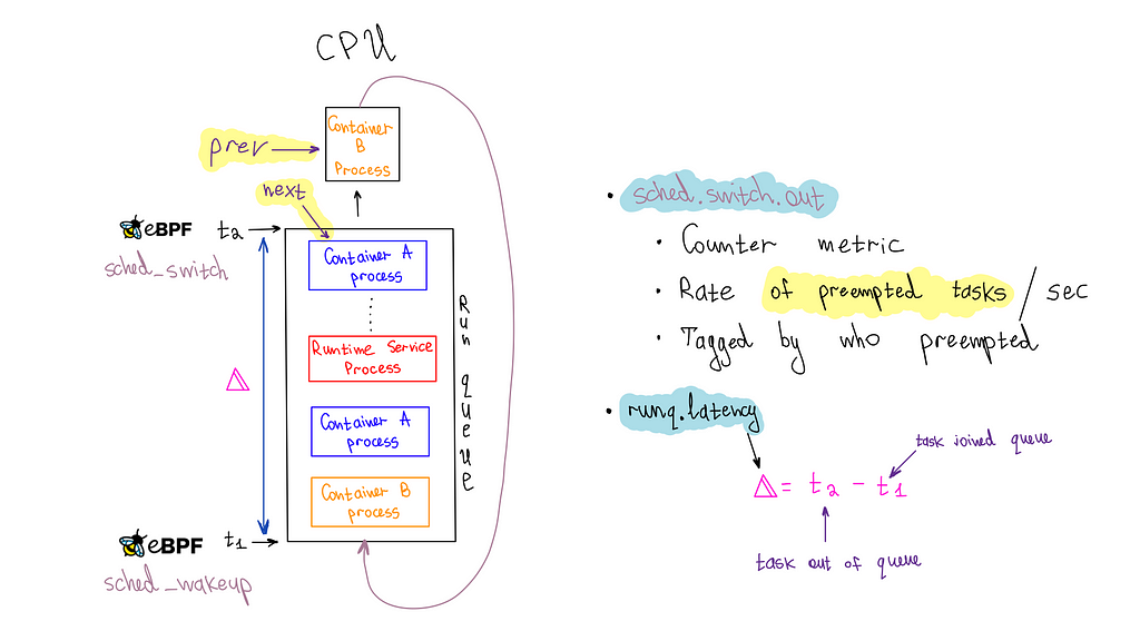
The sched_wakeup and sched_wakeup_new hooks are invoked when a process changes state from 'sleeping' to 'runnable.' They let us identify when a process is ready to run and is waiting for CPU time. During this event, we generate a timestamp and store it in an eBPF hash map using the process ID as the key.

struct {
__uint(type, BPF_MAP_TYPE_HASH);
__uint(max_entries, MAX_TASK_ENTRIES);
__uint(key_size, sizeof(u32));
__uint(value_size, sizeof(u64));
} runq_lat SEC(".maps");

SEC("tp_btf/sched_wakeup")
int tp_sched_wakeup(u64 *ctx)
{
struct task_struct *task = (void *)ctx[0];
u32 pid = task->pid;
u64 ts = bpf_ktime_get_ns();

bpf_map_update_elem(&runq_lat, &pid, &ts, BPF_NOEXIST);
return 0;
}

Conversely, the sched_switch hook is triggered when the CPU switches between processes. This hook provides pointers to the process currently utilizing the CPU and the process about to take over. We use the upcoming task's process ID (PID) to fetch the timestamp from the eBPF map. This timestamp represents when the process entered the queue, which we had previously stored. We then calculate the run queue latency by simply subtracting the timestamps.

SEC("tp_btf/sched_switch")
int tp_sched_switch(u64 *ctx)
{
struct task_struct *prev = (struct task_struct *)ctx[1];
struct task_struct *next = (struct task_struct *)ctx[2];
u32 prev_pid = prev->pid;
u32 next_pid = next->pid;

// fetch timestamp of when the next task was enqueued
u64 *tsp = bpf_map_lookup_elem(&runq_lat, &next_pid);
if (tsp == NULL) {
return 0; // missed enqueue
}

// calculate runq latency before deleting the stored timestamp
u64 now = bpf_ktime_get_ns();
u64 runq_lat = now - *tsp;

// delete pid from enqueued map
bpf_map_delete_elem(&runq_lat, &next_pid);
....

One of the advantages of eBPF is its ability to provide pointers to the actual kernel data structures representing processes or threads, also known as tasks in kernel terminology. This feature enables access to a wealth of information stored about a process. We required the process's cgroup ID to associate it with a container for our specific use case. However, the cgroup information in the struct is safeguarded by an RCU (Read Copy Update) lock.

To safely access this RCU-protected information, we can leverage kfuncs in eBPF. kfuncs are kernel functions that can be called from eBPF programs. There are kfuncs available to lock and unlock RCU read-side critical sections. These functions ensure that our eBPF program remains safe and efficient while retrieving the cgroup ID from the task struct.

void bpf_rcu_read_lock(void) __ksym;
void bpf_rcu_read_unlock(void) __ksym;

u64 get_task_cgroup_id(struct task_struct *task)
{
struct css_set *cgroups;
u64 cgroup_id;
bpf_rcu_read_lock();
cgroups = task->cgroups;
cgroup_id = cgroups->dfl_cgrp->kn->id;
bpf_rcu_read_unlock();
return cgroup_id;
}

Having the data ready, we must package it and send it to userspace. For this purpose, we chose the eBPF ring buffer. It is efficient, high-performing, and user-friendly. It can handle variable-length data records and allows data reading without necessitating extra memory copying or syscalls. However, the sheer amount of data points was causing the userspace program to use too much CPU, so we implemented a rate limiter in eBPF to sample the data effectively.

struct {
__uint(type, BPF_MAP_TYPE_RINGBUF);
__uint(max_entries, 256 * 1024);
} events SEC(".maps");

struct {
__uint(type, BPF_MAP_TYPE_PERCPU_HASH);
__uint(max_entries, MAX_TASK_ENTRIES);
__uint(key_size, sizeof(u64));
__uint(value_size, sizeof(u64));
} cgroup_id_to_last_event_ts SEC(".maps");

struct runq_event {
u64 prev_cgroup_id;
u64 cgroup_id;
u64 runq_lat;
u64 ts;
};

SEC("tp_btf/sched_switch")
int tp_sched_switch(u64 *ctx)
{
// ....
// The previous code
// ....

u64 prev_cgroup_id = get_task_cgroup_id(prev);
u64 cgroup_id = get_task_cgroup_id(next);

// per-cgroup-id-per-CPU rate-limiting
// to balance observability with performance overhead
u64 *last_ts =
bpf_map_lookup_elem(&cgroup_id_to_last_event_ts, &cgroup_id);
u64 last_ts_val = last_ts == NULL ? 0 : *last_ts;

// check the rate limit for the cgroup_id in consideration
// before doing more work
if (now - last_ts_val < RATE_LIMIT_NS) {
// Rate limit exceeded, drop the event
return 0;
}

struct runq_event *event;
event = bpf_ringbuf_reserve(&events, sizeof(*event), 0);

if (event) {
event->prev_cgroup_id = prev_cgroup_id;
event->cgroup_id = cgroup_id;
event->runq_lat = runq_lat;
event->ts = now;
bpf_ringbuf_submit(event, 0);
// Update the last event timestamp for the current cgroup_id
bpf_map_update_elem(&cgroup_id_to_last_event_ts, &cgroup_id,
&now, BPF_ANY);

}

return 0;
}

Our userspace application, developed in Go, processes events from the ring buffer to emit metrics to our metrics backend, Atlas. Each event includes a run queue latency sample with a cgroup ID, which we associate with running containers on the host. We categorize it as a system service if no such association is found. When a cgroup ID correlates with a container, we emit a percentile timer Atlas metric (runq.latency) for that container. We also increment a counter metric (sched.switch.out) to monitor preemptions occurring for the container's processes. Access to the prev_cgroup_id of the preempted process allows us to tag the metric with the cause of the preemption, whether it's due to a process within the same container (or cgroup), a process in another container, or a system service.

It's important to highlight that both the runq.latency metric and the sched.switch.out metrics are needed to determine if a container is affected by noisy neighbors, which is the goal we aim to achieve — relying solely on the runq.latency metric can lead to misconceptions. For example, if a container is at or over its cgroup CPU limit, the scheduler will throttle it, resulting in an apparent spike in run queue latency due to delays in the queue. If we were only to consider this metric, we might incorrectly attribute the performance degradation to noisy neighbors when it's actually because the container is hitting its CPU request limits. However, simultaneous spikes in both metrics, mainly when the cause is a different container or system process, clearly indicate a noisy neighbor issue.

A Noisy Neighbor Story

Below is the runq.latency metric for a server running a single container with ample CPU overhead. The 99th percentile averages 83.4µs (microseconds), serving as our baseline. Although there are some spikes reaching 400µs, the latency remains within acceptable parameters.

container1’s 99th percentile runq.latency averages 83µs (microseconds), with spikes up to 400µs, without adjacent containers. This serves as our baseline for a container not contending for CPU on a host.

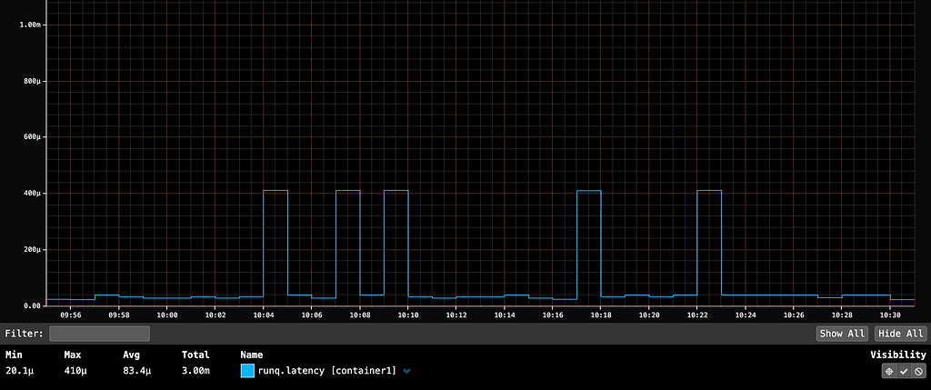
At 10:35, launching container2, which fully utilized all CPUs on the host, caused a significant 131-millisecond spike (131,000 microseconds) in container1's P99 run queue latency. This spike would be noticeable in the userspace application if it were serving HTTP traffic. If userspace app owners reported an unexplained latency spike, we could quickly identify the noisy neighbor issue through run queue latency metrics.

Launching container2 at 10:35, which maxes out all CPUs on the host, caused a 131-millisecond spike in container1’s P99 run queue latency due to increased preemptions by system processes. This indicates a noisy neighbor issue, where system services compete for CPU time with containers.

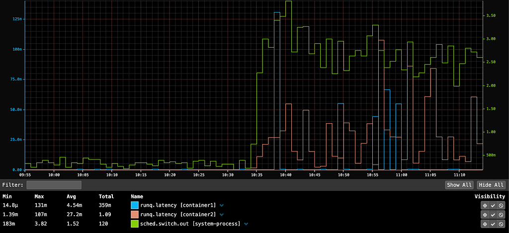
The sched.switch.out metric indicates that the spike was due to increased preemptions by system processes, highlighting a noisy neighbor issue where system services compete with containers for CPU time. Our metrics show that the noisy neighbors were actually system processes, likely triggered by container2 consuming all available CPU capacity.

Optimizing eBPF Code

We developed an open-source eBPF process monitor called bpftop to measure the overhead of eBPF code in this hot kernel path. Our estimates suggest that the instrumentation adds less than 600 nanoseconds to each sched_* hook. We conducted a performance analysis on a Java service running in a container, and the instrumentation did not introduce significant overhead. The performance variance with the run queue profiling code active versus inactive was not measurable in milliseconds.

During our research on how eBPF statistics are measured in the kernel, we identified an opportunity to improve its calculation. We submitted this patch, which was included in the Linux kernel 6.10 release.

Through trial and error and using bpftop, we identified several optimizations that helped maintain low overhead for this code:

  • We found that BPF_MAP_TYPE_HASH was the most performant for storing enqueued timestamps. Using BPF_MAP_TYPE_TASK_STORAGE resulted in nearly a twofold performance decline. BPF_MAP_TYPE_PERCPU_HASH was slightly less performant than BPF_MAP_TYPE_HASH, which was unexpected and requires further investigation.
  • The BPF_CORE_READ helper adds 20–30 nanoseconds per invocation. In the case of raw tracepoints, specifically those that are "BTF-enabled" (tp_btf/*), it is safe and more efficient to access the task struct members directly. Andrii Nakryiko recommends this approach in this blog post.
  • BPF_MAP_TYPE_LRU_HASH maps are 40–50 nanoseconds slower per operation than regular hash maps. Due to space concerns from PID churn, we initially used them for enqueued timestamps. We have since increased the map size, mitigating this risk.
  • The sched_switch, sched_wakeup, and sched_wakeup_new are all triggered for kernel tasks, which are identifiable by their PID of 0. We found monitoring these tasks unnecessary, so we implemented several early exit conditions and conditional logic to prevent executing costly operations, such as accessing BPF maps, when dealing with a kernel task. Notably, kernel tasks operate through the scheduler queue like any regular process.

Conclusion

Our findings highlight the value of low-overhead continuous instrumentation of the Linux kernel with eBPF. We have integrated these metrics into customer dashboards, enabling actionable insights and guiding multitenancy performance discussions. We can also now use these metrics to refine CPU isolation strategies to minimize the impact of noisy neighbors. Additionally, thanks to these metrics, we've gained deeper insights into the Linux scheduler.

This project has also deepened our understanding of eBPF technology and underscored the importance of tools like bpftop for optimizing eBPF code. As eBPF adoption increases, we foresee more infrastructure observability and business logic shifting to it. One promising project in this space is sched_ext, potentially revolutionizing how scheduling decisions are made and tailored to specific workload needs.


Noisy Neighbor Detection with eBPF was originally published in Netflix TechBlog on Medium, where people are continuing the conversation by highlighting and responding to this story.

Here is Why You Should Fully Populate Memory Channels on CPUs Featuring AMD EPYC Genoa

Post Syndicated from John Lee original https://www.servethehome.com/here-is-why-you-should-fully-populate-memory-channels-on-cpus-featuring-amd-epyc-genoa/

We test why you should populate your servers to fill all memory channels using an AMD EPYC 9004 Genoa 12-channel platform

The post Here is Why You Should Fully Populate Memory Channels on CPUs Featuring AMD EPYC Genoa appeared first on ServeTheHome.

Amazon SageMaker HyperPod introduces Amazon EKS support

Post Syndicated from Elizabeth Fuentes original https://aws.amazon.com/blogs/aws/amazon-sagemaker-hyperpod-introduces-amazon-eks-support/

Today, we are pleased to announce Amazon Elastic Kubernetes Service (EKS) support in Amazon SageMaker HyperPod — purpose-built infrastructure engineered with resilience at its core for foundation model (FM) development. This new capability enables customers to orchestrate HyperPod clusters using EKS, combining the power of Kubernetes with Amazon SageMaker HyperPod‘s resilient environment designed for training large models. Amazon SageMaker HyperPod helps efficiently scale across more than a thousand artificial intelligence (AI) accelerators, reducing training time by up to 40%.

Amazon SageMaker HyperPod now enables customers to manage their clusters using a Kubernetes-based interface. This integration allows seamless switching between Slurm and Amazon EKS for optimizing various workloads, including training, fine-tuning, experimentation, and inference. The CloudWatch Observability EKS add-on provides comprehensive monitoring capabilities, offering insights into CPU, network, disk, and other low-level node metrics on a unified dashboard. This enhanced observability extends to resource utilization across the entire cluster, node-level metrics, pod-level performance, and container-specific utilization data, facilitating efficient troubleshooting and optimization.

Launched at re:Invent 2023, Amazon SageMaker HyperPod has become a go-to solution for AI startups and enterprises looking to efficiently train and deploy large scale models. It is compatible with SageMaker’s distributed training libraries, which offer Model Parallel and Data Parallel software optimizations that help reduce training time by up to 20%. SageMaker HyperPod automatically detects and repairs or replaces faulty instances, enabling data scientists to train models uninterrupted for weeks or months. This allows data scientists to focus on model development, rather than managing infrastructure.

The integration of Amazon EKS with Amazon SageMaker HyperPod uses the advantages of Kubernetes, which has become popular for machine learning (ML) workloads due to its scalability and rich open-source tooling. Organizations often standardize on Kubernetes for building applications, including those required for generative AI use cases, as it allows reuse of capabilities across environments while meeting compliance and governance standards. Today’s announcement enables customers to scale and optimize resource utilization across more than a thousand AI accelerators. This flexibility enhances the developer experience, containerized app management, and dynamic scaling for FM training and inference workloads.

Amazon EKS support in Amazon SageMaker HyperPod strengthens resilience through deep health checks, automated node recovery, and job auto-resume capabilities, ensuring uninterrupted training for large scale and/or long-running jobs. Job management can be streamlined with the optional HyperPod CLI, designed for Kubernetes environments, though customers can also use their own CLI tools. Integration with Amazon CloudWatch Container Insights provides advanced observability, offering deeper insights into cluster performance, health, and utilization. Additionally, data scientists can use tools like Kubeflow for automated ML workflows. The integration also includes Amazon SageMaker managed MLflow, providing a robust solution for experiment tracking and model management.

At a high level, Amazon SageMaker HyperPod cluster is created by the cloud admin using the HyperPod cluster API and is fully managed by the HyperPod service, removing the undifferentiated heavy lifting involved in building and optimizing ML infrastructure. Amazon EKS is used to orchestrate these HyperPod nodes, similar to how Slurm orchestrates HyperPod nodes, providing customers with a familiar Kubernetes-based administrator experience.

Let’s explore how to get started with Amazon EKS support in Amazon SageMaker HyperPod
I start by preparing the scenario, checking the prerequisites, and creating an Amazon EKS cluster with a single AWS CloudFormation stack following the Amazon SageMaker HyperPod EKS workshop, configured with VPC and storage resources.

To create and manage Amazon SageMaker HyperPod clusters, I can use either the AWS Management Console or AWS Command Line Interface (AWS CLI). Using the AWS CLI, I specify my cluster configuration in a JSON file. I choose the Amazon EKS cluster created previously as the orchestrator of the SageMaker HyperPod Cluster. Then, I create the cluster worker nodes that I call “worker-group-1”, with a private Subnet, NodeRecovery set to Automatic to enable automatic node recovery and for OnStartDeepHealthChecks I add InstanceStress and InstanceConnectivity to enable deep health checks.

cat > eli-cluster-config.json << EOL
{
    "ClusterName": "example-hp-cluster",
    "Orchestrator": {
        "Eks": {
            "ClusterArn": "${EKS_CLUSTER_ARN}"
        }
    },
    "InstanceGroups": [
        {
            "InstanceGroupName": "worker-group-1",
            "InstanceType": "ml.p5.48xlarge",
            "InstanceCount": 32,
            "LifeCycleConfig": {
                "SourceS3Uri": "s3://${BUCKET_NAME}",
                "OnCreate": "on_create.sh"
            },
            "ExecutionRole": "${EXECUTION_ROLE}",
            "ThreadsPerCore": 1,
            "OnStartDeepHealthChecks": [
                "InstanceStress",
                "InstanceConnectivity"
            ],
        },
  ....
    ],
    "VpcConfig": {
        "SecurityGroupIds": [
            "$SECURITY_GROUP"
        ],
        "Subnets": [
            "$SUBNET_ID"
        ]
    },
    "ResilienceConfig": {
        "NodeRecovery": "Automatic"
    }
}
EOL

You can add InstanceStorageConfigs to provision and mount an additional Amazon EBS volumes on HyperPod nodes.

To create the cluster using the SageMaker HyperPod APIs, I run the following AWS CLI command:

aws sagemaker create-cluster \ 
--cli-input-json file://eli-cluster-config.json

The AWS command returns the ARN of the new HyperPod cluster.

{
"ClusterArn": "arn:aws:sagemaker:us-east-2:ACCOUNT-ID:cluster/wccy5z4n4m49"
}

I then verify the HyperPod cluster status in the SageMaker Console, awaiting until the status changes to InService.

Alternatively, you can check the cluster status using the AWS CLI running the describe-cluster command:

aws sagemaker describe-cluster --cluster-name my-hyperpod-cluster

Once the cluster is ready, I can access the SageMaker HyperPod cluster nodes. For most operations, I can use kubectl commands to manage resources and jobs from my development environment, using the full power of Kubernetes orchestration while benefiting from SageMaker HyperPod’s managed infrastructure. On this occasion, for advanced troubleshooting or direct node access, I use AWS Systems Manager (SSM) to log into individual nodes, following the instructions in the Access your SageMaker HyperPod cluster nodes page.

To run jobs on the SageMaker HyperPod cluster orchestrated by EKS, I follow the steps outlined in the Run jobs on SageMaker HyperPod cluster through Amazon EKS page. You can use the HyperPod CLI and the native kubectl command to find avaible HyperPod clusters and submit training jobs (Pods). For managing ML experiments and training runs, you can use Kubeflow Training Operator, Kueue and Amazon SageMaker-managed MLflow.

Finally, in the SageMaker Console, I can view the Status and Kubernetes version of recently added EKS clusters, providing a comprehensive overview of my SageMaker HyperPod environment.

And I can monitor cluster performance and health insights using Amazon CloudWatch Container.

Things to know
Here are some key things you should know about Amazon EKS support in Amazon SageMaker HyperPod:

Resilient Environment – This integration provides a more resilient training environment with deep health checks, automated node recovery, and job auto-resume. SageMaker HyperPod automatically detects, diagnoses, and recovers from faults, allowing you to continually train foundation models for weeks or months without disruption. This can reduce training time by up to 40%.

Enhanced GPU Observability Amazon CloudWatch Container Insights provides detailed metrics and logs for your containerized applications and microservices. This enables comprehensive monitoring of cluster performance and health.

Scientist-Friendly Tool – This launch includes a custom HyperPod CLI for job management, Kubeflow Training Operators for distributed training, Kueue for scheduling, and integration with SageMaker Managed MLflow for experiment tracking. It also works with SageMaker’s distributed training libraries, which provide Model Parallel and Data Parallel optimizations to significantly reduce training time. These libraries, combined with auto-resumption of jobs, enable efficient and uninterrupted training of large models.

Flexible Resource Utilization – This integration enhances developer experience and scalability for FM workloads. Data scientists can efficiently share compute capacity across training and inference tasks. You can use your existing Amazon EKS clusters or create and attach new ones to HyperPod compute, bring your own tools for job submission, queuing and monitoring.

To get started with Amazon SageMaker HyperPod on Amazon EKS, you can explore resources such as the SageMaker HyperPod EKS Workshop, the aws-do-hyperpod project, and the awsome-distributed-training project. This release is generally available in the AWS Regions where Amazon SageMaker HyperPod is available except Europe(London). For pricing information, visit the Amazon SageMaker Pricing page.

This blog post was a collaborative effort. I would like to thank Manoj Ravi, Adhesh Garg, Tomonori Shimomura, Alex Iankoulski, Anoop Saha, and the entire team for their significant contributions in compiling and refining the information presented here. Their collective expertise was crucial in creating this comprehensive article.

– Eli.

Migrate Delta tables from Azure Data Lake Storage to Amazon S3 using AWS Glue

Post Syndicated from Nitin Kumar original https://aws.amazon.com/blogs/big-data/migrate-delta-tables-from-azure-data-lake-storage-to-amazon-s3-using-aws-glue/

Organizations are increasingly using a multi-cloud strategy to run their production workloads. We often see requests from customers who have started their data journey by building data lakes on Microsoft Azure, to extend access to the data to AWS services. Customers want to use a variety of AWS analytics, data, AI, and machine learning (ML) services like AWS Glue, Amazon Redshift, and Amazon SageMaker to build more cost-efficient, performant data solutions harnessing the strength of individual cloud service providers for their business use cases.

In such scenarios, data engineers face challenges in connecting and extracting data from storage containers on Microsoft Azure. Customers typically use Azure Data Lake Storage Gen2 (ADLS Gen2) as their data lake storage medium and store the data in open table formats like Delta tables, and want to use AWS analytics services like AWS Glue to read the delta tables. AWS Glue, with its ability to process data using Apache Spark and connect to various data sources, is a suitable solution for addressing the challenges of accessing data across multiple cloud environments.

AWS Glue is a serverless data integration service that makes it straightforward to discover, prepare, and combine data for analytics, ML, and application development. AWS Glue custom connectors allow you to discover and integrate additional data sources, such as software as a service (SaaS) applications and your custom data sources. With just a few clicks, you can search for and subscribe to connectors from AWS Marketplace and begin your data preparation workflow in minutes.

In this post, we explain how you can extract data from ADLS Gen2 using the Azure Data Lake Storage Connector for AWS Glue. We specifically demonstrate how to import data stored in Delta tables in ADLS Gen2. We provide step-by-step guidance on how to configure the connector, author an AWS Glue ETL (extract, transform, and load) script, and load the extracted data into Amazon Simple Storage Service (Amazon S3).

Azure Data Lake Storage Connector for AWS Glue

The Azure Data Lake Storage Connector for AWS Glue simplifies the process of connecting AWS Glue jobs to extract data from ADLS Gen2. It uses the Hadoop’s FileSystem interface and the ADLS Gen2 connector for Hadoop. The Azure Data Lake Storage Connector for AWS Glue also includes the hadoop-azure module, which lets you run Apache Hadoop or Apache Spark jobs directly with data in ADLS. When the connector is added to the AWS Glue environment, AWS Glue loads the library from the Amazon Elastic Container Registry (Amazon ECR) repository during initialization (as a connector). When AWS Glue has internet access, the Spark job in AWS Glue can read from and write to ADLS.

With the availability of the Azure Data Lake Storage Connector for AWS Glue in AWS Marketplace, an AWS Glue connection makes sure you have the required packages to use in your AWS Glue job.

For this post, we use the Shared Key authentication method.

Solution overview

In this post, our objective is to migrate a product table named sample_delta_table, which currently resides in ADLS Gen2, to Amazon S3. To accomplish this, we use AWS Glue, the Azure Data Lake Storage Connector for AWS Glue, and AWS Secrets Manager to securely store the Azure shared key. We employed an AWS Glue serverless ETL job, configured with the connector, to establish a connection to ADLS using shared key authentication over the public internet. After the table is migrated to Amazon S3, we use Amazon Athena to query Delta Lake tables.

The following architecture diagram illustrates how AWS Glue facilitates data ingestion from ADLS.

Prerequisites

You need the following prerequisites:

Configure your ADLS Gen2 account in Secrets Manager

Complete the following steps to create a secret in Secrets Manager to store the ADLS credentials:

  1. On the Secrets Manager console, choose Store a new secret.
  2. For Secret type, select Other type of secret.
  3. Enter the key accountName for the ADLS Gen2 storage account name.
  4. Enter the key accountKey for the ADLS Gen2 storage account key.
  5. Enter the key container for the ADLS Gen2 container.
  6. Leave the rest of the options as default and choose Next.

  1. Enter a name for the secret (for example, adlstorage_credentials).
  2. Choose Next.
  3. Complete the rest of the steps to store the secret.

Subscribe to the Azure Data Lake Storage Connector for AWS Glue

The Azure Data Lake Storage Connector for AWS Glue simplifies the process of connecting AWS Glue jobs to extract data from ADLS Gen2. The connector is available as an AWS Marketplace offering.

Complete the following steps to subscribe to the connector:

  1. Log in to your AWS account with the necessary permissions.
  2. Navigate to the AWS Marketplace page for the Azure Data Lake Storage Connector for AWS Glue.
  3. Choose Continue to Subscribe.
  4. Choose Continue to Configuration after reading the EULA.

  1. For Fulfilment option, choose Glue 4.0.
  2. For Software version, choose the latest software version.
  3. Choose Continue to Launch.

Create a custom connection in AWS Glue

After you’re subscribed to the connector, complete the following steps to create an AWS Glue connection based on it. This connection will be added to the AWS Glue job to make sure the connector is available and the data store connection information is accessible to establish a network pathway.

To create the AWS Glue connection, you need to activate the Azure Data Lake Storage Connector for AWS Glue on the AWS Glue Studio console. After you choose Continue to Launch in the previous steps, you’re redirected to the connector landing page.

  1. In the Configuration details section, choose Usage instructions.
  2. Choose Activate the Glue connector from AWS Glue Studio.

The AWS Glue Studio console allows the option to either activate the connector or activate it and create the connection in one step. For this post, we choose the second option.

  1. For Connector, confirm Azure ADLS Connector for AWS Glue 4.0 is selected.
  2. For Name, enter a name for the connection (for example, AzureADLSStorageGen2Connection).
  3. Enter an optional description.
  4. Choose Create connection and activate connector.

The connection is now ready for use. The connector and connection information is visible on the Data connections page of the AWS Glue console.


Read Delta tables from ADLS Gen2 using the connector in an AWS Glue ETL job

Complete the following steps to create an AWS Glue job and configure the AWS Glue connection and job parameter options:

  1. On the AWS Glue console, choose ETL jobs in the navigation pane.
  2. Choose Author code with a script editor and choose Script editor.
  3. Choose Create script and go to the Job details section.
  4. Update the settings for Name and IAM role.
  5. Under Advanced properties, add the AWS Glue connection AzureADLSStorageGen2Connection created in previous steps.
  1. For Job parameters, add the key --datalake-formats with the value as delta.
  1. Use the following script to read the Delta table from ADLS. Provide the path to where you have Delta table files in your Azure storage account container and the S3 bucket for writing delta files to the output S3 location.
from pyspark.sql import SparkSession
from delta.tables import *
import boto3
import json

spark = SparkSession.builder.getOrCreate()

sm = boto3.client('secretsmanager')
response = sm.get_secret_value(SecretId="adlstorage_credentials")
value = json.loads(response['SecretString'])
account_name_sparkconfig = f"fs.azure.account.key.{value['accountName']}.dfs.core.windows.net"
account_name = value['accountName']
account_key = value['accountKey']
container_name = value['container']
path = f"abfss://{container_name}@{account_name}.dfs.core.windows.net/path-to-delta-table-files/"
s3DeltaTablePath="s3://yourdatalakebucketname/deltatablepath/"

# Method: Shared Key  
spark.conf.set(account_name_sparkconfig, account_key)

# Read delta table from ADLS gen2 storage
df = spark.read.format("delta").load(path)

# Write delta table to S3 path.
if DeltaTable.isDeltaTable(spark,s3DeltaTablePath):
    s3deltaTable = DeltaTable.forPath(spark,s3DeltaTablePath)
    print("Merge to existing s3 delta table")
    (s3deltaTable.alias("target")
        .merge(df.alias("source"), "target.product_id = source.product_id")
        .whenMatchedUpdateAll()
        .whenNotMatchedInsertAll()
        .execute()
    )
else:
    print("Create delta table to S3.")
    df.write.format("delta").save(s3DeltaTablePath)
  1. Choose Run to start the job.
  2. On the Runs tab, confirm the job ran successfully.
  3. On the Amazon S3 console, verify the delta files in the S3 bucket (Delta table path).
  4. Create a database and table in Athena to query the migrated Delta table in Amazon S3.

You can accomplish this step using an AWS Glue crawler. The crawler can automatically crawl your Delta table stored in Amazon S3 and create the necessary metadata in the AWS Glue Data Catalog. Athena can then use this metadata to query and analyze the Delta table seamlessly. For more information, see Crawl Delta Lake tables using AWS Glue crawlers.

CREATE DATABASE deltadb;
CREATE EXTERNAL TABLE deltadb.sample_delta_table
LOCATION 's3://yourdatalakebucketname/deltatablepath/'
TBLPROPERTIES ('table_type'='DELTA');

12. Query the Delta table:

SELECT * FROM "deltadb"."sample_delta_table" limit 10;

By following the steps outlined in the post, you have successfully migrated a Delta table from ADLS Gen2 to Amazon S3 using an AWS Glue ETL job.

Read the Delta table in an AWS Glue notebook

The following are optional steps if you want to read the Delta table from ADLS Gen2 in an AWS Glue notebook:

  1. Create a notebook and run the following code in the first notebook cell to configure the AWS Glue connection and --datalake-formats in an interactive session:
%idle_timeout 30
%glue_version 4.0
%worker_type G.1X
%number_of_workers 5
%connections AzureADLSStorageGen2Connection
%%configure
{
   "--datalake-formats": "delta"
}

  1. Run the following code in a new cell to read the Delta table stored in ADLS Gen 2. Provide the path to where you have delta files in an Azure storage account container and the S3 bucket for writing delta files to Amazon S3.
from pyspark.sql import SparkSession
from delta.tables import *
import boto3
import json

spark = SparkSession.builder.getOrCreate()

sm = boto3.client('secretsmanager')
response = sm.get_secret_value(SecretId="adlstorage_credentials")
value = json.loads(response['SecretString'])
account_name_sparkconfig = f"fs.azure.account.key.{value['accountName']}.dfs.core.windows.net"
account_name = value['accountName']
account_key = value['accountKey']
container_name = value['container']
path = f"abfss://{container_name}@{account_name}.dfs.core.windows.net/path-to-delta-table-files/"
s3DeltaTablePath="s3://yourdatalakebucketname/deltatablepath/"

# Method: Shared Key  
spark.conf.set(account_name_sparkconfig, account_key)

# Read delta table from ADLS gen2 storage
df = spark.read.format("delta").load(path)

# Write delta table to S3 path.
if DeltaTable.isDeltaTable(spark,s3DeltaTablePath):
    s3deltaTable = DeltaTable.forPath(spark,s3DeltaTablePath)
    print("Merge to existing s3 delta table")
    (s3deltaTable.alias("target")
        .merge(df.alias("source"), "target.product_id = source.product_id")
        .whenMatchedUpdateAll()
        .whenNotMatchedInsertAll()
        .execute()
    )
else:
    print("Create delta table to S3.")
    df.write.format("delta").save(s3DeltaTablePath)

Clean up

To clean up your resources, complete the following steps:

  1. Remove the AWS Glue job, database, table, and connection:
    1. On the AWS Glue console, choose Tables in the navigation pane, select sample_delta_table, and choose Delete.
    2. Choose Databases in the navigation pane, select deltadb, and choose Delete.
    3. Choose Connections in the navigation pane, select AzureADLSStorageGen2Connection, and on the Actions menu, choose Delete.
  2. On the Secrets Manager console, choose Secrets in the navigation pane, select adlstorage_credentials, and on the Actions menu, choose Delete secret.
  3. If you are no longer going to use this connector, you can cancel the subscription to the connector:
    1. On the AWS Marketplace console, choose Manage subscriptions.
    2. Select the subscription for the product that you want to cancel, and on the Actions menu, choose Cancel subscription.
    3. Read the information provided and select the acknowledgement check box.
    4. Choose Yes, cancel subscription.
  4. On the Amazon S3 console, delete the data in the S3 bucket that you used in the previous steps. 

You can also use the AWS Command Line Interface (AWS CLI) to remove the AWS Glue and Secrets Manager resources. Remove the AWS Glue job, database, table, connection, and Secrets Manager secret with the following command:

aws glue delete-job —job-name <your_job_name>
aws glue delete-connection —connection-name <your_connection_name>
aws secretsmanager delete-secret —secret-id <your_secretsmanager_id>
aws glue delete-table --database-name deltadb --name sample_delta_table
aws glue delete-database --name deltadb

Conclusion

In this post, we demonstrated a real-world example of migrating a Delta table from Azure Delta Lake Storage Gen2 to Amazon S3 using AWS Glue. We used an AWS Glue serverless ETL job, configured with an AWS Marketplace connector, to establish a connection to ADLS using shared key authentication over the public internet. Additionally, we used Secrets Manager to securely store the shared key and seamlessly integrate it within the AWS Glue ETL job, providing a secure and efficient migration process. Lastly, we provided guidance on querying the Delta Lake table from Athena.

Try out the solution for your own use case, and let us know your feedback and questions in the comments.


About the Authors

Nitin Kumar is a Cloud Engineer (ETL) at Amazon Web Services, specialized in AWS Glue. With a decade of experience, he excels in aiding customers with their big data workloads, focusing on data processing and analytics. He is committed to helping customers overcome ETL challenges and develop scalable data processing and analytics pipelines on AWS. In his free time, he likes to watch movies and spend time with his family.

Shubham Purwar is a Cloud Engineer (ETL) at AWS Bengaluru, specialized in AWS Glue and Amazon Athena. He is passionate about helping customers solve issues related to their ETL workload and implement scalable data processing and analytics pipelines on AWS. In his free time, Shubham loves to spend time with his family and travel around the world.

Pramod Kumar P is a Solutions Architect at Amazon Web Services. With 19 years of technology experience and close to a decade of designing and architecting connectivity solutions (IoT) on AWS, he guides customers to build solutions with the right architectural tenets to meet their business outcomes.

Madhavi Watve is a Senior Solutions Architect at Amazon Web Services, providing help and guidance to a broad range of customers to build highly secure, scalable, reliable, and cost-efficient applications on the cloud. She brings over 20 years of technology experience in software development and architecture and is data analytics specialist.

Swathi S is a Technical Account Manager with the Enterprise Support team in Amazon Web Services. She has over 6 years of experience with AWS on big data technologies and specializes in analytics frameworks. She is passionate about helping AWS customers navigate the cloud space and enjoys assisting with design and optimization of analytics workloads on AWS.

Evaluating sample Amazon Redshift data sharing architecture using Redshift Test Drive and advanced SQL analysis

Post Syndicated from Ayan Majumder original https://aws.amazon.com/blogs/big-data/evaluating-sample-amazon-redshift-data-sharing-architecture-using-redshift-test-drive-and-advanced-sql-analysis/

With the launch of Amazon Redshift Serverless and the various provisioned instance deployment options, customers are looking for tools that help them determine the most optimal data warehouse configuration to support their Amazon Redshift workloads.

Amazon Redshift is a widely used, fully managed, petabyte-scale data warehouse service. Tens of thousands of customers use Amazon Redshift to process exabytes of data every day to power their analytics workloads.

Redshift Test Drive is a tool hosted on the GitHub repository that let customers evaluate which data warehouse configurations options are best suited for their workload. The Test Drive Workload Replicator utility consists of scripts that can be used to extract the workload queries from your source warehouse audit logs and replay them on a target warehouse you launched. The Test Drive Configuration Comparison utility automates this process by deploying target Amazon Redshift warehouses and orchestrating the replay of the source workload through a combination of AWS CloudFormation and AWS StepFunctions.

Both utilities unload the performance metrics from the replay of the source workload on the target configuration(s) to Amazon Simple Storage Service (Amazon S3), which is used as a storage to store the performance metrics. Although the Replay Analysis UI and Configuration Comparison utility can provide a preliminary performance comparison, many customers want to dig deeper by analyzing the raw data themselves.

The walkthrough illustrates an example workload replayed on a single Amazon Redshift data warehouse and data sharing architecture using the Workload Replicator utility, the output of which will be used to evaluate the performance of the workload.

Use case overview

For the sample use case, we assumed we have an existing 2 x ra3.4xlarge provisioned data warehouse that currently runs extract, transform, and load (ETL), ad hoc, and business intelligence (BI) queries. We’re interested in breaking these workloads apart using data sharing into a 32 base Redshift Processing Unit (RPU) Serverless producer running ETL and a 64 base RPU Serverless consumer running the BI workload. We used Workload Replicator to replay the workload on a replica baseline of the source and target data sharing configuration as specified in the tutorial. The following image shows the process flow.

Generating and accessing Test Drive metrics

The results of Amazon Redshift Test Drive can be accessed using an external schema for analysis of a replay. Refer to the Workload Replicator README and the Configuration Comparison README for more detailed instructions to execute a replay using the respective tool.

The external schema for analysis is automatically created with the Configuration Comparison utility, in which case you can proceed directly to the SQL analysis in the Deploy the QEv2 SQL Notebook and analyze workload section. If you use Workload Replicator, however, the external schema is not created automatically, and therefore needs to be configured as a prerequisite to the SQL analysis. We demonstrate in the following walkthrough how the external schema can be set up, using sample analysis of the Data Sharing use case.

Executing Test Drive Workload Replicator for data sharing

To execute Workload Replicator, use Amazon Elastic Compute Cloud (Amazon EC2) to run the automation scripts used to extract the workload from the source.

Configure Amazon Redshift Data Warehouse

  1. Create a snapshot following the guidance in the Amazon Redshift Management Guide.
  2. Enable audit logging following the guidance in Amazon Redshift Management Guide.
  3. Enable the user activity logging of the source cluster following the guidance Amazon Redshift Management Guide.

Enabling logging requires a change of the parameter group. Audit logging needs to be enabled prior to the workload that will be replayed because this is where the connections and SQL queries of the workload will be extracted from.

  1. Launch the baseline replica from the snapshot by restoring a 2 node ra3.4xlarge provisioned cluster from the snapshot.
  2. Launch the producer warehouse by restoring the snapshot to a 32 RPU serverless namespace.
  3. The consumer should not contain the schema and tables that will be shared from the producer. You can launch the 64 RPU Serverless consumer either from the snapshot and then drop the relevant objects, or you can create a new 64 RPU Serverless consumer warehouse and recreate consumer users.
  4. Create a datashare from the producer to the consumer and add the relevant objects.

Data share objects can be read using two mechanisms: using three-part notation (database.schema.table), or by creating an external schema pointing to a shared schema and querying that using two-part notation (external_schema.table). Because we want to seamlessly run the source workload, which uses two-part notation on the local objects, this post demonstrates the latter approach. For each schema shared from the producer, run the following command on the consumer:

CREATE EXTERNAL SCHEMA schema_name 
FROM REDSHIFT DATABASE ‘datashare_database_name’ SCHEMA ‘schema_name’;

Make sure to use the same schema name as the source for the external schema. Also, if any queries are run on the public schema, drop the local public schema first before creating the external equivalent.

  1. Grant usage on the schema for any relevant users.

Configure Redshift Test Drive Workload Replicator

  1. Create an S3 bucket to store the artifacts required by the utility (such as the metrics, extracted workload, and output data from running UNLOAD commands).
  2. Launch the following three types of EC2 instances using the recommended configuration of m5.8xlarge, 32GB of SSD storage, and Amazon Linux AMI:
    1. Baseline instance
    2. Target-producer instance
    3. Target-consumer instance

Make sure you can connect to the EC2 instance to run the utility.

  1. For each instance, install the required libraries by completing the following steps from the GitHub repository:
    a. 2.i
    b. 2.ii (if an ODBC driver should be used—the default is the Amazon Redshift Python driver)
    c. 2.iii
    d. 2.iv
    e. 2.v
  2. Create an AWS Identity and Access Management (IAM) role for the EC2 instances to access the Amazon Redshift warehouses, to read from the S3 audit logging bucket, and with both read and write access to the new S3 bucket created for storing replay artifacts.
  3. If you are going to run COPY and UNLOAD commands, create an IAM role with access to the S3 buckets required, and attach it to the Amazon Redshift warehouses that will execute the load and unload.

In this example, the IAM role is attached to the baseline replica and producer warehouses because these will be executing the ETL processes. The utility will update UNLOAD commands to unload data to a bucket you define, which as a best practice should be the bucket created for S3 artifacts. Write permissions need to be granted to the Amazon Redshift warehouse for this location.

Run Redshift Test Drive Workload Replicator

  1. Run aws configure on the EC2 instances and populate the default Region with the Region the utility is being executed in.
  2. Extract only needs to be run once, so connect to the baseline EC2 instance and run vi config/extract.yaml to open the extract.yaml file and configure the extraction details (select i to begin configuring elements, then use escape to leave edit mode and :wq! to leave vi). For more details on the parameters, see Configure parameters.

The following code is an example of a configured extract that unloads the logs for a half hour window to the Test Drive artifacts bucket and updates COPY commands to run with the POC Amazon Redshift role.

Configuration Extract File

  1. Run make extract to extract the workload. When completed, make note of the folder created at the path specified for the workload_location parameter in the extract (s3://testdriveartifacts/myworkload/Extraction_xxxx-xx-xxTxx:xx:xx.xxxxxx+00:00).
  2. On the same baseline EC2 instance that will run the full workload on the source replica, run vi config/replay.yaml and configure the details with the workload location copied in the previous step 3 and the baseline warehouse endpoint. (See additional details on the parameters Configure parameters to run an extract job. The values after the analysis_iam_role parameter can be left as the default).

The following code is an example for the beginning of a replay configuration for the source replica.

Config Reply File

  1. On the EC2 instance that will run the target-producer workload, run vi config/replay.yaml. Configure the details with the workload location copied in the previous step 3, the producer warehouse endpoint and other configuration as in step 4. In order to replay only the producer workload, add the appropriate users to include or exclude for the filters parameter.

The following code is an example of the filters used to exclude the BI workload from the producer.

Producer Configuration

  1. On the EC2 instance that will run the target-consumer workload, run vi config/replay.yaml and configure the details with the workload location copied in the previous step 3, the consumer warehouse endpoint, and appropriate filters as for step 5. The same users that were excluded on the producer workload replay should be included in the consumer workload replay.

The following is an example of the filters used to only run the BI workload from the consumer.

Consumer Configuration

  1. Run make replay on the baseline instance, target-producer instance, and target-consumer instance simultaneously to run the workload on the target warehouses.

Analyze the Workload Replicator output

  1. Create the folder structure in the S3 bucket that was created in the previous step.
'{comparison_stats_s3_path}/{what_if_timestamp}/{cluster_identifier}/'

For comparison_stats_s3_path, enter the S3 bucket and path name. For what_if_timestamp, enter the replay start time. For cluster_identifier, enter the target cluster name for easy identification.

The following screenshot shows

Configuration of S3

  1. Use the following script to unload system table data for each target cluster to a corresponding Amazon S3 target path that was created previously in the baseline Redshift cluster using QEv2.
UNLOAD ($$
SELECT a.*,Trim(u.usename) as username FROM sys_query_history a , pg_user u
WHERE a.user_id = u.usesysid
and a.start_time > to_timestamp('{what_if_timestamp}','YYYY-MM- DD-HH24-MI-SS')
$$) TO '{comparison_stats_s3_path}/{what_if_timestamp}/{cluster_identifier}/'
FORMAT AS PARQUET PARALLEL OFF ALLOWOVERWRITE 
IAM_ROLE '{redshift_iam_role}';

For what_if_timestamp, enter the replay start time. For comparison_stats_s3_path, enter the S3 bucket and path name. For cluster_identifier, enter the target cluster name for easy identification. For redshift_iam_role, enter the Amazon Resource Name (ARN) of the Redshift IAM role for the target cluster.

Unload File

  1. Create an external schema in Amazon Redshift with the name comparison_stats.
CREATE EXTERNAL SCHEMA comparison_stats from DATA CATALOG
DATABASE 'redshift_config_comparison'
IAM_ROLE '{redshift-iam-role}'
CREATE EXTERNAL DATABASE IF NOT EXISTS;
  1. Create an external table in Amazon Redshift with the name redshift_config_comparision_aggregate based on the Amazon S3 file location.
CREATE EXTERNAL TABLE comparison_stats.redshift_config_comparision_aggregate 
(user_id int,
query_id bigint,
query_label VARCHAR,
transaction_id bigint,
session_id int,
database_name VARCHAR,
query_type VARCHAR,
status VARCHAR,
result_cache_hit boolean,
start_time timestamp,
end_time timestamp,
elapsed_time bigint,
queue_time bigint,
execution_time bigint,
error_message VARCHAR,
returned_rows bigint,
returned_bytes bigint,
query_text VARCHAR,
redshift_version VARCHAR,
usage_limit VARCHAR,
compute_type VARCHAR,
compile_time bigint,
planning_time bigint,
lock_wait_time bigint,
username VARCHAR)
PARTITIONED BY (cluster_identifier VARCHAR)
STORED AS PARQUET
LOCATION '{comparison_stats_s3_path}/{what_if_timestamp}';
  1. After creating a partitioned table, alter the table using the following statement to register partitions to the external catalog.

When you add a partition, you define the location of the subfolder on Amazon S3 that contains the partition data. Run that statement for each cluster identifier.

ALTER TABLE comparison_stats.redshift_config_comparision_aggregate 
ADD PARTITION (cluster_identifier='{cluster_identifier}')
LOCATION '{comparison_stats_s3_path}/{what_if_timestamp}/{cluster_identifier}/';

Example:

ALTER TABLE comparison_stats.redshift_config_comparision_aggregate 
ADD PARTITION (cluster_identifier='baseline-ra3-4xlarge-2')
LOCATION 's3://workload-replicator-redshift/2024-03-05-21-00-00/baseline-ra3-4xlarge-2/';
ALTER TABLE comparison_stats.redshift_config_comparision_aggregate 
ADD PARTITION (cluster_identifier='producer-serverless32RPU')
LOCATION 's3://workload-replicator-redshift/2024-03-05-21-00-00/producer-serverless32RPU/';
ALTER TABLE comparison_stats.redshift_config_comparision_aggregate 
ADD PARTITION (cluster_identifier='consumer-serverless64RPU')
LOCATION 's3://workload-replicator-redshift/2024-03-05-21-00-00/consumer-serverless64RPU/';

Deploy the QEv2 SQL Notebook and analyze workload

In this section, we analyze the queries that were replayed in both the baseline and target clusters. We analyze the workload based on the common queries that are executed in the baseline and target clusters.

  1. Download the analysis notebook from Amazon S3.
  2. Import the notebook into the baseline Redshift clusters using QEv2. For guidance, refer to the Authoring and running notebooks.
  3. Create the stored procedure common_queries_sp in the same database that was used to create the external schema.
  4. The stored procedure will create a view called common_queries by querying the external table redshift_config_comparison_aggregate that was created in previous steps.

The view will identify the queries common to both the baseline and target clusters as mentioned in the notebook.

  1. Execute the stored procedure by passing the cluster identifiers for the baseline and target clusters as parameters to the stored procedure.

For this post, we passed the baseline and producer cluster identifier as the parameters. Passing the cluster identifiers as parameters will retrieve the data only for those specific clusters.

Once the common_queries view is created, you can perform further analysis using subsequent queries that are available in the notebook. If you have more than one target cluster, you can follow the same analysis process for each one. For this post, we have two target clusters: producer and consumer. We first performed the analysis between the baseline and producer clusters, then repeated the same process to analyze the data for the baseline versus consumer clusters.

To analyze our workload, we will use the sys_query_history view. We frequently use several columns from this view, including the following:

  • elapsed_time: The end-to-end time of the query run
  • execution_time: The time the query spent running. In the case of a SELECT query, this also includes the return time.
  • compile_time: The time the query spent compiling

For more information on sys_query_history, refer to SYS_QUERY_HISTORY in the Amazon Redshift Database Developer Guide. The following table shows the descriptions of the analysis queries.

Name of the query Description
1 Overall workload by user Count of common queries between baseline and target clusters based on user
2 Overall workload by query type Count of common queries between baseline and target clusters based on query type
3 Overall workload comparison (in seconds) Compare the overall workload between the baseline and target clusters by analyzing the execution time, compile time, and elapsed time
4 Percentile workload comparison The percentage of queries that perform at or below that runtime (for example, p50_s having the value of 5 seconds means 50% of queries in that workload were 5 seconds or faster)
5 Number of improve/degrade/stay same queries The number of queries degraded/stayed the same/improved when comparing the elapsed time between the baseline and target clusters
6 Degree of query-level performance change (proportion) The degree of change of the query from the baseline to target relative to the baseline performance
7 Comparison by query type (in seconds) Compare the elapsed time of different query types such as SELECT, INSERT, and COPY commands between the baseline cluster and target cluster
8 Top 10 slowest running queries (in seconds) Top 10 slowest queries between the baseline and target cluster by comparing the elapsed time of both clusters
9 Top 10 improved queries (in seconds) The top 10 queries with the most improved elapsed time when comparing the baseline cluster to the target cluster

Sample Results analysis

In our example, the overall workload improvement for workload isolation architecture using data sharing for ETL workload between baseline and producer is 858 seconds (baseline_elapsed_timetarget_elapsed_time) for the sample TPC data, as shown in the following screenshots.

Baseline vs Producer Analysis

Baseline vs Producer Analysis Grpah

The overall workload improvement for workload isolation architecture using data sharing for BI workload between baseline and consumer is 1148 seconds (baseline_elapsed_timetarget_elapsed_time) for sample TPC data, as shown in the following screenshots.

Baseline vs Consumer Analysis

Baseline vs Consumer Analysis Graph

Cleanup

Complete the following steps to clean up your resources:

  1. Delete the Redshift provisioned replica cluster and the two Redshift serverless endpoints (32 RPU and 64 RPU)
  2. Delete the S3 bucket used to store the artifacts
  3. Delete the baseline, target-producer, and target-consumer EC2 instances
  4. Delete the IAM role created for the EC2 instances to access Redshift clusters and S3 buckets
  5. Delete the IAM roles created for Amazon Redshift warehouses to access S3 buckets for COPY and UNLOAD commands

Conclusion

In this post, we walked you through the process of testing workload isolation architecture using Amazon Redshift Data Sharing and Test Drive utility. We demonstrated how you can use SQL for advanced price performance analysis and compare different workloads on different target Redshift cluster configurations. We encourage you to evaluate your Amazon Redshift data sharing architecture using the Redshift Test Drive tool. Use the provided SQL script to analyze the price-performance of your Amazon Redshift cluster.


About the Authors

Ayan Majumder is an Analytics Specialist Solutions Architect at AWS. His expertise lies in designing robust, scalable, and efficient cloud solutions for customers. Beyond his professional life, he derives joy from traveling, photography, and outdoor activities.

Ekta Ahuja is an Amazon Redshift Specialist Solutions Architect at AWS. She is passionate about helping customers build scalable and robust data and analytics solutions. Before AWS, she worked in several different data engineering and analytics roles. Outside of work, she enjoys landscape photography, traveling, and board games.

Julia BeckJulia Beck is an Analytics Specialist Solutions Architect at AWS. She is passionate about supporting customers in validating and optimizing analytics solutions by architecting proof of concept workloads designed to meet their specific needs.

A good day to trie-hard: saving compute 1% at a time

Post Syndicated from Kevin Guthrie original https://blog.cloudflare.com/pingora-saving-compute-1-percent-at-a-time


Cloudflare’s global network handles a lot of HTTP requests – over 60 million per second on average. That in and of itself is not news, but it is the starting point to an adventure that started a few months ago and ends with the announcement of a new open-source Rust crate that we are using to reduce our CPU utilization, enabling our CDN to handle even more of the world’s ever-increasing Web traffic. 

Motivation

Let’s start at the beginning. You may recall a few months ago we released Pingora (the heart of our Rust-based proxy services) as an open-source project on GitHub. I work on the team that maintains the Pingora framework, as well as Cloudflare’s production services built upon it. One of those services is responsible for the final step in transmitting users’ (non-cached) requests to their true destination. Internally, we call the request’s destination server its “origin”, so our service has the (unimaginative) name of “pingora-origin”.

One of the many responsibilities of pingora-origin is to ensure that when a request leaves our infrastructure, it has been cleaned to remove the internal information we use to route, measure, and optimize traffic for our customers. This has to be done for every request that leaves Cloudflare, and as I mentioned above, it’s a lot of requests. At the time of writing, the rate of requests leaving pingora-origin (globally) is 35 million requests per second. Any code that has to be run per-request is in the hottest of hot paths, and it’s in this path that we find this code and comment:

// PERF: heavy function: 1.7% CPU time
pub fn clear_internal_headers(request_header: &mut RequestHeader) {
    INTERNAL_HEADERS.iter().for_each(|h| {
        request_header.remove_header(h);
    });
}

This small and pleasantly-readable function consumes more than 1.7% of pingora-origin’s total cpu time. To put that in perspective, the total cpu time consumed by pingora-origin is 40,000 compute-seconds per second. You can think of this as 40,000 saturated CPU cores fully dedicated to running pingora-origin. Of those 40,000, 1.7% (680) are only dedicated to evaluating clear_internal_headers. The function’s heavy usage and simplicity make it seem like a great place to start optimizing.

Benchmarking

Benchmarking the function shown above is straightforward because we can use the wonderful criterion Rust crate. Criterion provides an api for timing rust code down to the nanosecond by aggregating multiple isolated executions. It also provides feedback on how the performance improves or regresses over time. The input for the benchmark is a large set of synthesized requests with a random number of headers with a uniform distribution of internal vs. non-internal headers. With our tooling and test data we find that our original clear_internal_headers function runs in an average of 3.65µs. Now for each new method of clearing headers, we can measure against the same set of requests and get a relative performance difference. 

Reducing Reads

One potentially quick win is to invert how we find the headers that need to be removed from requests. If you look at the original code, you can see that we are evaluating request_header.remove_header(h) for each header in our list of internal headers, so 100+ times. Diagrammatically, it looks like this:


Since an average request has significantly fewer than 100 headers (10-30), flipping the lookup direction should reduce the number of reads while yielding the same intersection. Because we are working in Rust (and because retain does not exist for http::HeaderMap yet), we have to collect the identified internal headers in a separate step before removing them from the request. Conceptually, it looks like this:


Using our benchmarking tool, we can measure the impact of this small change, and surprisingly this is already a substantial improvement. The runtime improves from 3.65µs to 1.53µs. That’s a 2.39x speed improvement for our function. We can calculate the theoretical CPU percentage by multiplying the starting utilization by the ratio of the new and old times: 1.71% * 1.53 / 3.65 = 0.717%. Unfortunately, if we subtract that from the original 1.71% that only equates to saving 1.71% – 0.717% = 0.993% of the total CPU time. We should be able to do better. 

Searching Data Structures

Now that we have reorganized our function to search a static set of internal headers instead of the actual request, we have the freedom to choose what data structure we store our header name in simply by changing the type of INTERNAL_HEADER_SET.

pub fn clear_internal_headers(request_header: &mut RequestHeader) {
   let to_remove = request_header
       .headers
       .keys()
       .filter_map(|name| INTERNAL_HEADER_SET.get(name))
       .collect::<Vec<_>>();


   to_remove.into_iter().for_each(|k| {
       request_header.remove_header(k);
   });

Our first attempt used std::HashMap, but there may be other data structures that better suit our needs. All computer science students were taught at some point that hash tables are great because they have constant-time asymptotic behavior, or O(1), for reading. (If you are not familiar with big O notation, it is a way to express how an algorithm consumes a resource, in this case time, as the input size changes.) This means no matter how large the map gets, reads always take the same amount of time. Too bad this is only partially true. In order to read from a hash table, you have to compute the hash. Computing a hash for strings requires reading every byte, so while read time for a hashmap is constant over the table’s size, it’s linear over key length. So, our goal is to find a data structure that is better than O(L) where L is the length of the key.

There are a few common data structures that provide for reads that have read behavior that meets our criteria. Sorted sets like BTreeSet use comparisons for searching, and that makes them logarithmic over key length O(log(L)), but they are also logarithmic in size too. The net effect is that even very fast sorted sets like FST work out to be a little (50 ns) slower in our benchmarks than the standard hashmap.

State machines like parsers and regex are another common tool for searching for strings, though it’s hard to consider them data structures. These systems work by accepting input one unit at a time and determining on each step whether or not to keep evaluating. Being able to make these determinations at every step means state machines are very fast to identify negative cases (i.e. when a string is not valid or not a match). This is perfect for us because only one or two headers per request on average will be internal. In fact, benchmarking an implementation of clear_internal_headers using regular expressions clocks in as taking about twice as long as the hashmap-based solution. This is impressively fast given that regexes, while powerful, aren’t known for their raw speed. This approach feels promising – we just need something in between a data structure and a state machine.

That’s where the trie comes in.

Don’t Just Trie

A trie (pronounced like “try” or “tree”) is a type of tree data structure normally used for prefix searches or auto-complete systems over a known set of strings. The structure of the trie lends itself to this because each node in the trie represents a substring of characters found in the initial set. The connections between the nodes represent the characters that can follow a prefix. Here is a small example of a trie built from the words: “and”, “ant”, “dad”, “do”, & “dot”. 


The root node represents an empty string prefix, so the two lettered edges directed out of it are the only letters that can appear as the first letter in the list of strings, “a” and “d”. Subsequent nodes have increasingly longer prefixes until the final valid words are reached. This layout should make it easy to see how a trie could be useful for quickly identifying strings that are not contained. Even at the root node, we can eliminate any strings that are presented that do not start with “a” or “d”. This paring down of the search space on every step gives reading from a trie the O(log(L)) we were looking for … but only for misses. Hits within a trie are still O(L), but that’s okay, because we are getting misses over 90% of the time.

Benchmarking a few trie implementations from crates.io was disheartening. Remember, most tries are used in response to keyboard events, so optimizing them to run in the hot path of tens of millions of requests per second is not a priority. The fastest existing implementation we found was radix_trie, but it still clocked in at a full microsecond slower than hashmap. The only thing left to do was write our own implementation of a trie that was optimized for our use case.

Trie Hard

And we did! Today we are announcing trie-hard. The repository gives a full description of how it works, but the big takeaway is that it gets its speed from storing node relationships in the bits of unsigned integers and keeping the entire tree in a contiguous chunk of memory. In our benchmarks, we found that trie-hard reduced the average runtime for clear_internal_headers to under a microsecond (0.93µs). We can reuse the same formula from above to calculate the expected CPU utilization for trie-hard to be 1.71% * 3.65 / 0.93 = 0.43% That means we have finally achieved and surpassed our goal by reducing the compute utilization of pingora-origin by 1.71% – 0.43% =  1.28%

Up until now we have been working only in theory and local benchmarking. What really matters is whether our benchmarking reflects real-life behavior. Trie-hard has been running in production since July 2024, and over the course of this project we have been collecting performance metrics from the running production of pingora-origin using a statistical sampling of its stack trace over time. Using this technique, the CPU utilization percentage of a function is estimated by the percent of samples in which the function appears. If we compare the sampled performance of the different versions of clear_internal_headers, we can see that the results from the performance sampling closely match what our benchmarks predicted.

Implementation

Stack trace samples containing clear_internal_headers

Actual CPU Usage (%)

Predicted CPU Usage (%)

Original 

19 / 1111

1.71

n/a

Hashmap

9 / 1103

0.82

0.72

trie-hard

4 / 1171

0.34

0.43

Conclusion

Optimizing functions and writing new data structures is cool, but the real conclusion for this post is that knowing where your code is slow and by how much is more important than how you go about optimizing it. Take a moment to thank your observability team (if you’re lucky enough to have one), and make use of flame graphs or any other profiling and benchmarking tool you can. Optimizing operations that are already measured in microseconds may seem a little silly, but these small improvements add up.

[$] The trouble with iowait

Post Syndicated from corbet original https://lwn.net/Articles/989272/

CPU scheduling is a challenging job; since it inherently requires making
guesses about what the demands on the system will be in the future, it
remains reliant on heuristics, despite ongoing efforts to remove them.
Some of those heuristics take special note of tasks that are (or appear to
be) waiting for fast I/O operations. There is some unhappiness, though,
with how this factor is used, leading to a couple of patches taking rather
different approaches to improve the situation.

Radicle 1.0 released

Post Syndicated from corbet original https://lwn.net/Articles/989605/

Version 1.0
of the Radicle development platform has been released.

Radicle 1.0 represents the culmination of years of experimentation
and hard work from our team and community, where we set out to
ensure that free and open source software ecosystems can flourish
without having to rely on the whims of Big Tech. We designed
Radicle with a first-principles approach, as a natural extension to
Git, expanding it to work in a collaborative, local-first,
peer-to-peer setting.

LWN looked at Radicle in March.

Rapid7 Named a Leader in IDC MarketScape: Worldwide SIEM for SMB

Post Syndicated from Meaghan Buchanan original https://blog.rapid7.com/2024/09/10/rapid7-named-a-leader-in-idc-marketscape-worldwide-siem-for-smb/

Rapid7 Named a Leader in IDC MarketScape: Worldwide SIEM for SMB

Rapid7 is excited to share we have been recognized as a Leader in the IDC MarketScape: Worldwide SIEM for SMB 2024 Vendor Assessment (doc #US52038824, September 2024). We want to thank our customers for their partnership, feedback, and trust, all of which continue to guide how we build and innovate toward our mission to deliver command of the attack surface and keep security teams ready for whatever comes next.

Rapid7 Named a Leader in IDC MarketScape: Worldwide SIEM for SMB

What sets InsightIDR apart from other SIEMs

When we entered this space almost nine years ago, we were driven by customers who were bogged down by the complexity and ineffectiveness of traditional SIEMs. Unfortunately, challenging deployments, constant tuning, unmanageable alerts, and inflated total cost of ownership continue to plague many SIEM users today – making it impossible to maximize utility of these products and challenging team effectiveness.

InsightIDR is different.

1. Intuitive deployment and UI to maximize efficiency

A strong SIEM product can be the nucleus of the SOC – helping to harmonize otherwise disparate data into a clear picture of the attack surface and relevant insights. Unfortunately, many SIEMs are off track from the start due to:

  • Complex deployments
  • High operational overhead
  • Tedious configuration work that consumes team resources

InsightIDR’s cloud-native, SaaS delivery makes it fast and easy to get started without the burdens of heavy infrastructure management, while ensuring you have the scale to grow with your business when you need it. Easily identify the priority data to ingest and quickly start collecting the right information with:

  • Intuitive onboarding wizards
  • Flexibility to leverage our native data collection (endpoint agent, network sensor, collectors)
  • Ability to connect your extended security ecosystem with vast integrations
  • Auto-enrichment of logs with user and asset details via our attribution engine
  • Custom log parsers
  • In-product guidance

With 13 months of readily searchable data and flexible search modes that can accommodate your most experienced to your most junior analysts, InsightIDR puts your data to work for you – not the other way around.

2. Optimized for modern threat detection

While collecting the right telemetry is a critical piece of unifying the attack surface, too many SIEMs are overly indexed on log aggregation. Lost in logs and making sense of data, teams can lose sight of the thing that matters most: staying ahead of an attack.

InsightIDR has taken a detections-first approach to SIEM and is proud to deliver a robust library of out-of-the-box detections that customers can trust and use as a starting line to augment their own threat intelligence and detections engineering programs. With coverage across all phases of the MITRE ATT&CK framework, this is the same detections library used in the field by our own Rapid7 MDR SOC experts – ensuring strong signal-to-noise detections and constant curation to keep teams ahead of emergent threats.

This library marries both AI-charged user and attacker behavioral detections alongside known IOC coverage to ensure you are ready for both evasive, headline-making unknown threats as well as recognized adversary TTPs. Detections are comprehensive across the modern attack surface – from endpoint-to-cloud – and can easily be customized or added onto so customers can feel confident they are covered no matter where threats begin.

3. Ready to respond across the attack surface

With a rapidly expanding attack surface, all teams are challenged to ensure they know how to investigate and respond effectively to alerts. It’s harder than ever to understand lateral movement and the full blast radius, so it’s critical to ensure analysts have enough context to take action – and the right playbooks and tools in place to execute when they’re ready to do so.

InsightIDR is built around making sure analyst teams are ready to respond effectively to threats every time. Highly correlated investigation timelines unify related alerts and events across the security ecosystem to give a cohesive view of an attack and all relevant evidence in one place.

Integrated access to the Velociraptor DFIR framework enables teams to quickly query fleets of endpoints to assess and understand the blast radius of an attack. And when it’s time to take action, alerts are paired with descriptive guidance and recommendations vetted by our own SOC experts. Fully embedded SOAR capabilities and pre-built playbooks accelerate readiness and time-to-respond. We understand the friction and toll that noisy alerts and complex investigations can take on SOC teams; InsightIDR reduces this burnout and the likelihood of analyst churn by decreasing cycles and friction across investigation workflows – creating happier and more effective teams.

4. Tangible return on investment

Probably one of the things that many SIEMs are most notorious for is high and unpredictable costs and resource consumption – with few results to show for it. Traditional ingestion-based models have always been a challenge for security teams – and it’s getting even more difficult as the attack surface becomes increasingly dynamic.

InsightIDR is available in a number of flexible packages designed around real customer needs and security journeys. Our Threat Complete product marries InsightIDR with our leading vulnerability management to deliver proactive, threat-informed risk management to further reduce noise and strengthen security posture.

Predictable, asset-based pricing across our packages means no surprise charges to explain to your C-Suite or Board. And executive dashboards help you share insights and show progress to your wider organization to be able to show how you are advancing your threat detection and incident response program.

We are proud to be a Leader

Thank you to the IDC MarketScape for this recognition. We are proud to be named a Leader, but we are always most proud of the thousands of customers and partners across the globe who trust Rapid7 at the center of their security program. To learn more, access a complimentary excerpt of the IDC MarketScape or start exploring InsightIDR.

Security updates for Tuesday

Post Syndicated from corbet original https://lwn.net/Articles/989602/

Security updates have been issued by Debian (cacti), Fedora (aardvark-dns, expat, and firefox), Mageia (ffmpeg, ntfs-3g, and vim), Oracle (emacs, glib2, java-11-openjdk, and qt5-qtbase), Red Hat (emacs, python-setuptools, python3.11, python3.11-setuptools, python3.12-setuptools, python3.9, and python39:3.9), Slackware (netatalk), SUSE (buildah, expat, java-1_8_0-ibm, kanidm, kernel, and postgresql16), and Ubuntu (netty, php7.0, php7.2, tiff, and webkit2gtk).

Experience AI at UNESCO’s Digital Learning Week

Post Syndicated from Ben Garside original https://www.raspberrypi.org/blog/experience-ai-unescos-digital-learning-week/

Last week, we were honoured to attend UNESCO’s Digital Learning Week conference to present our free Experience AI resources and how they can help teachers demystify AI for their learners.  

A group of educators at a UNESCO conference.

The conference drew a worldwide audience in-person and online to hear about the work educators and policy makers are doing to support teachers’ use of AI tools in their teaching and learning. Speaker after speaker reiterated that the shared goal of our work is to support learners to become critical consumers and responsible creators of AI systems.

In this blog, we share how our conference talk demonstrated the use of Experience AI for pursuing this globally shared goal, and how the Experience AI resources align with UNESCO’s newly launched AI competency framework for students.

Presenting the design principles behind Experience AI

Our talk about Experience AI, our learning programme developed with Google DeepMind, focused on the research-informed approach we are taking in our resource development. Specifically, we spoke about three key design principles that we embed in the Experience AI resources:

Firstly, using AI and machine learning to solve problems requires learners and educators to think differently to traditional computational thinking and use a data-driven approach instead, as laid out in the research around computational thinking 2.0.

Secondly, every word we use in our teaching about AI is important to help young people form accurate mental models about how AI systems work. In particular, we focused our examples around the need to avoid anthropomorphising language when we describe AI systems. Especially given that some developers produce AI systems with the aim to make them appear human-like in their design and outputs, it’s important that young people understand that AI systems are in fact built and designed by humans.

Thirdly we described how we used the SEAME framework we adapted from work by Jane Waite (Raspberry Pi Foundation) and Paul Curzon (Queen Mary University, London) to categorise hundreds of AI education resources and inform the design of our Experience AI resources. The framework offers a common language for educators when assessing the content of resources, and when supporting learners to understand the different aspects of AI systems. 

By presenting our design principles, we aimed to give educators, policy makers, and attendees from non-governmental organisations practical recommendations and actionable considerations for designing learning materials on AI literacy.   

How Experience AI aligns with UNESCO’s new AI competency framework for students

At Digital Learning Week, UNESCO launched two AI competency frameworks:

  • A framework for students, intended to help teachers around the world with integrating AI tools in activities to engage their learners
  • A framework for teachers, “defining the knowledge, skills, and values teachers must master in the age of AI”

AI competency framework for students

We have had the chance to map the Experience AI resources to UNESCO’s AI framework for students at a high level, finding that the resources cover 10 of the 12 areas of the framework (see image below).

An adaptation of a summary table from UNESCO’s new student competency framework (CC-BY-SA 3.0 IGO), highlighting the 10 areas covered by our Experience AI resources

For instance, throughout the Experience AI resources runs a thread of promoting “citizenship in the AI era”: the social and ethical aspects of AI technologies are highlighted in all the lessons and activities. In this way, they provide students with the foundational knowledge of how AI systems work, and where they may work badly. Using the resources, educators can teach their learners core AI and machine learning concepts and make these concepts concrete through practical activities where learners create their own models and critically evaluate their outputs. Importantly, by learning with Experience AI, students not only learn to be responsible users of AI tools, but also to consider fairness, accountability, transparency, and privacy when they create AI models.  

Teacher competency framework for AI 

UNESCO’s AI competency framework for teachers outlines 15 competencies across 5 dimensions (see image below).  We enjoyed listening to the launch panel members talk about the strong ambitions of the framework as well as the realities of teachers’ global and local challenges. The three key messages of the panel were:

  • AI will not replace the expertise of classroom teachers
  • Supporting educators to build AI competencies is a shared responsibility
  • Individual countries’ education systems have different needs in terms of educator support

All three messages resonate strongly with the work we’re doing at the Raspberry Pi Foundation. Supporting all educators is a fundamental part of our resource development. For example, Experience AI offers everything a teacher with no technical background needs to deliver the lessons, including lesson plans, videos, worksheets and slide decks. We also provide a free online training course on understanding AI for educators. And in our work with partner organisations around the world, we adapt and translate Experience AI resources so they are culturally relevant, and we organise locally delivered teacher professional development. 

A summary table from UNESCO’s new teacher competency framework (CC-BY-SA 3.0 IGO)

 The teachers’ competency framework is meant as guidance for educators, policy makers, training providers, and application developers to support teachers in using AI effectively, and in helping their learners gain AI literacy skills. We will certainly consult the document as we develop our training and professional development resources for teachers further.

Towards AI literacy for all young people

Across this year’s UNESCO’s Digital Learning Week, we saw that the role of AI in education took centre stage across the presentations and the informal conversations among attendees. It was a privilege to present our work and see how well Experience AI was received, with attendees recognising that our design principles align with the values and principles in UNESCO’s new AI competency frameworks.

A conference table setup with a pair of headphones resting on top of a UNESCO brochure.

We look forward to continuing this international conversation about AI literacy and working in aligned ways to support all young people to develop a foundational understanding of AI technologies.

The post Experience AI at UNESCO’s Digital Learning Week appeared first on Raspberry Pi Foundation.

Monitoring Zabbix Security Advisories

Post Syndicated from Brian van Baekel original https://blog.zabbix.com/monitoring-zabbix-security-advisories/28672/

Zabbix plays a crucial role in monitoring all kinds of “things” – IoT devices, domains, cloud infrastructures and more. It can also be integrated with third-party solutions – for example, with Oxidized for configuration backup monitoring. Given the nature of Zabbix, it usually contains a lot of confidential information as well as (more importantly) some kind of elevated access to network elements while being used by operators, engineers, and customers. This requires that Zabbix as a product should be as secure as possible.

Zabbix has upped their security game and is actively working with HackerOne to take full advantage of the reach of their global community by providing a bug bounty program. And though it doesn’t happen too often, from time to time a security issue arises in Zabbix or one of its dependencies, warranting the release of a Security Advisory.

The issue

Zabbix typically releases a Security Advisory and might even assign a CVE to the issue. Cool, that is what we expect from reputable software developers. They even inform their customers with support contracts before publishing the advisory, in order to allow them to patch installations beforehand.

Unfortunately, if you don’t have a support contract you’re expected to find out about these security advisories on your own, either by monitoring the Security Advisory page or by monitoring the published CVEs for Zabbix. NIST has a public API that can be used and that works well, but the issue with CVE’s is that they are often incomplete and thus useless. For example, CVE-2024-22119 contains far less information than the advisory.

Currently, Zabbix does not publish an API for their Security Advisories. There is the public tracker which contains all entries and can be queried via API, but because it is unstructured text, it is really hard to parse.

The solution

We want to automatically be notified of new security advisories, and the only data source that contains all data in a structured way is the Zabbix Security Advisory page. However, structured doesn’t mean easily parseable – in fact, it is just raw HTML. We could try to solve this issue in Zabbix, but the easier solution in this case is to scrape the page and generate a JSON file which then can be parsed by Zabbix to achieve our goal, which is automated notifications of new advisories.

Webscraping

We’ve chosen to scrape the Zabbix site using Rust, utilizing the Scraper crate to parse the HTML and flesh out the relevant parts we want. Without going into too much detail, the interesting information is stored in 2 tables, one with the table-simple class applied and one with the table-vertical class applied. Using CSS selectors (which is what the Scraper crate requires), we can retrieve the information we want.

This information is then stored in a struct, which gets added to a hashmap. The result is stored in a vector, which is added to a struct, which eventually is used to generate the JSON we require. Phew.

The resulting JSON is easily parseable by Zabbix:

{
  "last_updated": {
    "secs": ,
    "nanos": ,
  },
  "reports": [
    _list of reports_
  ]
}

The ‘reports’ array contains one entry per advisory, and each entry has the following layout. Unsurprisingly, this closely matches the information that is available on the Zabbix Security Advisory page:

    {
      "_zbxref_": {
        "zbxref": "_zbxref_",
        "cveref": "CVE-XXXX-XXXX",
        "score": X.X,
        "synopsis": "_synopsis_",
        "description": "_description_",
        "vectors": "_vectors_",
        "resolution": "_resolution_",
        "workaround": "_workaround_",
        "acknowledgement": "_acknowledgement_",
        "components": [
          _list of components_,
          _list of components_
        ],
        "affected_version": [
          {
            "affected": "_version_",
            "fixed": "_version_"
          }
        ]
      }
    }

Now, we could provide you with the code of the scraping tool and wish you good luck with making sure the tool runs every X hours and somehow, somewhere stores the resulting JSON for Zabbix to parse. That would be the easy way out, right?

Instead, we’ve chosen to host the Rust program as an AWS Lambda function, triggered every 2 hours by the AWS EventBridge Scheduler and with some code added to the Rust program (function?) to upload the resulting JSON to an AWS S3 bucket. This chain of AWS products not only makes sure that our cloud bill increases, but also guarantees we don’t have to host (and maintain!) anything ourselves.

The result? Just one HTTP GET away…

Template

TL;DR: Download the template here.

Now that the data is available in JSON, it’s fairly easy to parse it using Zabbix. Using the HTTP Agent data collection, we download the JSON from AWS. The URI is stored in the {$ZBX_ADVISORY_URI} macro, which allows for easy modification. By default, it points to the JSON file hosted on AWS S3. This retrieval is done by the Retrieve the Zabbix Security Advisories item, which acts as the source for every other operation. It retrieves the JSON every hour, and with the JSON being generated every 2 hours, the maximum delay between Zabbix publishing a new advisory and you getting it into Zabbix is 3 hours.

The retrieve the Zabbix Security Advisories item acts as a master item for the Last Updated item. This item uses a JSONPath preprocessing step to flesh out the information we want: $.last_updated.secs. The resulting data is stored as unixtime so that we mere mortals can easily read when the last update of the JSON file was performed.

A trigger is configured for this item to ensure that the JSON file isn’t too old. The trigger JSON Feed is out of date has the following expression:
last(/Zabbix Security Advisories/zbx_sec.last_updated)>{$ZBX_ADVISORY_UPDATE_INTERVAL}*{$ZBX_ADVISORY_UPDATE_THRESHOLD}

By default, {$ZBX_ADVISORY_UPDATE_INTERVAL} is set to 2 hours (which is the interval the file gets updated by our tool) and {$ZBX_ADVISORY_UPDATE_THRESHOLD} is set to 3. So, when the JSON file hasn’t been updated within the last 6 hours, this trigger will trigger.

The item Number of advisories uses the same principle, where a JSONPath preprocessing step is used to flesh out the information we want: $.reports. However, as $.reports is an array, we can use functions on it. In this case .length(), which returns an integer. This number is used in the associated trigger A new Zabbix Security Advisory has been published, which simply triggers when the value changes.

This is all very cool, but the JSON has a lot more information, including details about each report. In order to get these details into Zabbix, we use a discovery rule to ‘loop’ through the JSON and create items based on what we’ve discovered: Discover Advisories. This rule uses (again) a JSONPath preprocessing step to get the details we want: $.reports[*][*]. Based on the resulting data (which is a single report in this case), 2 LLD Macros are assigned: {#ZBXREF} – based on the JSONpath $.zbxref and {{#CVEREF} – based on the JSONpath $.cveref.

For each discovered report, 8 items are created. They all work using the same principle, so I will only describe one: Advisory {#ZBXREF} / {#CVEREF} – Acknowledgement. This item uses the master item Zabbix Security Advisories, just like all other items described so far. JSONPath is once again used to get the information we want. The expression $.reports[*][“{#ZBXREF}”].acknowledgement.first() provides exactly what we need, where we combine a LLD macro ({#ZBXREF}) and a JSONpath function (.first()) to first ‘select’ the correct advisory in the JSON and then retrieve the value.

All other 7 items work like this, and there is only one exception: Advisory {#ZBXREF} / {#CVEREF} – Components. The ‘components’ value in the JSON file is actually an array with 1 or more items, describing which components might be affected. But we cannot store arrays in Zabbix, so we use another preprocessing step to convert the array into a string. A few lines of Javascript is all we need:

components = JSON.parse(value);
return components.toString();

First, we parse the JSON input (‘value’) into an array, only to apply the javascript .toString() function on it. The toString method of arrays calls join() internally, which joins the array and returns one string containing each array element separated by commas, which is exactly what we want: a string, separated by commas.

To make working with these advisories easier, each item has the component tag applied, with the value zabbix_security. If the item belongs to an advisory, the advisory tag is added with the value of {#ZBXREF} (which is the advisory number/name). That way, we can easily filter on all Zabbix Security items, filter on all items for a single advisory, and (to make things even better) the type tag is also applied, with the actual type being ‘workaround’ or ‘description.’ This allows for filtering on all Zabbix Security items, of the type ‘score’ (et cetera) to easily gain insight into the different advisories and their score, synopsis, description, components, et cetera.

Dashboard

The tags on the items allow for filtering, but with Zabbix 7.0 we can use all great new nifty features, such as the Item Navigator widget combined with the Item Value widget. Let’s take a look at what configuring such a dashboard might look like if you set up the Item Navigator widget as follows:

Item Navigator configuration

And then ‘link’ the Item Value widget to it:

You should get a somewhat decent dashboard. It isn’t perfect (given that the Item Value widget only seems to be able to display a single line of text) but it’s something.

Disclaimer

Though we use this functionality ourselves, this all comes without any guarantee. The technology used to retrieve data (screen scraping) is mediocre at best and could break at any moment if and when Zabbix changes the layout of their page.

The post Monitoring Zabbix Security Advisories appeared first on Zabbix Blog.

Unveiling the process: The creation of our powerful campaign builder

Post Syndicated from Grab Tech original https://engineering.grab.com/the-creation-of-our-powerful-campaign-builder

In a previous blog, we introduced Trident, Grab’s internal marketing campaign platform. Trident empowers our marketing team to configure If This, Then That (IFTTT) logic and processes real-time events based on that.

While we mainly covered how we scaled up the system to handle large volumes of real-time events, we did not explain the implementation of the event processing mechanism. This blog will fill up this missing piece. We will walk you through the various processing mechanisms supported in Trident and how they were built.

Base building block: Treatment

In our system, we use the term “treatment” to refer to the core unit of a full IFTTT data structure. A treatment is an amalgamation of three key elements – an event, conditions (which are optional), and actions. For example, consider a promotional campaign that offers “100 GrabPoints for completing a ride paid with GrabPay Credit”. This campaign can be transformed into a treatment in which the event is “ride completion”, the condition is “payment made using GrabPay Credit”, and the action is “awarding 100 GrabPoints”.

Data generated across various Kafka streams by multiple services within Grab forms the crux of events and conditions for a treatment. Trident processes these Kafka streams, treating each data object as an event for the treatments. It evaluates the set conditions against the data received from these events. If all conditions are met, Trident then executes the actions.

Figure 1. Trident processes Kafka streams as events for treatments.

When the Trident user interface (UI) was first established, campaign creators had to grasp the treatment concept and configure the treatments accordingly. As we improved the UI, it became more user-friendly.

Building on top of treatment

Campaigns can be more complex than the example we provided earlier. In such scenarios, a single campaign may need transformation into several treatments. All these individual treatments are categorised under what we refer to as a “treatment group”. In this section, we discuss features that we have developed to manage such intricate campaigns.

Counter

Let’s say we have a marketing campaign that “rewards users after they complete 4 rides”. For this requirement, it’s necessary for us to keep track of the number of rides each user has completed. To make this possible, we developed a capability known as counter.

On the backend, a single counter setup translates into two treatments.

Treatment 1:

  • Event: onRideCompleted
  • Condition: N/A
  • Action: incrementUserStats

Treatment 2:

  • Event: onProfileUpdate
  • Condition: Ride Count == 4
  • Action: awardReward

In this feature, we introduce a new event, onProfileUpdate. The incrementUserStats action in Treatment 1 triggers the onProfileUpdate event following the update of the user counter. This allows Treatment 2 to consume the event and perform subsequent evaluations.

Figure 2. The end-to-end evaluation process when using the Counter feature.

When the onRideCompleted event is consumed, Treatment 1 is evaluated which then executes the incrementUserStat action. This action increments the user’s ride counter in the database, gets the latest counter value, and publishes an onProfileUpdate event to Kafka.

There are also other consumers that listen to onProfileUpdate events. When this event is consumed, Treatment 2 is evaluated. This process involves verifying whether the Ride Count equals to 4. If the condition is satisfied, the awardReward action is triggered.

This feature is not limited to counting the number of event occurrences only. It’s also capable of tallying the total amount of transactions, among other things.

Delay

Another feature available on Trident is a delay function. This feature is particularly beneficial in situations where we want to time our actions based on user behaviour. For example, we might want to give a ride voucher to a user three hours after they’ve ordered a ride to a theme park. The intention for this is to offer them a voucher they can use for their return trip.

On the backend, a delay setup translates into two treatments. Given the above scenario, the treatments are as follows:

Treatment 1:

  • Event: onRideCompleted
  • Condition: Dropoff Location == Universal Studio
  • Action: scheduleDelayedEvent

Treatment 2:

  • Event: onDelayedEvent
  • Condition: N/A
  • Action: awardReward

We introduce a new event, onDelayedEvent, which Treatment 1 triggers during the scheduleDelayedEvent action. This is made possible by using Simple Queue Service (SQS), given its built-in capability to publish an event with a delay.

Figure 3. The end-to-end evaluation process when using the Delay feature.

The maximum delay that SQS supports is 15 minutes; meanwhile, our platform allows for a delay of up to x hours. To address this limitation, we publish the event multiple times upon receiving the message, extending the delay by another 15 minutes each time, until it reaches the desired delay of x hours.

Limit

The Limit feature is used to restrict the number of actions for a specific campaign or user within that campaign. This feature can be applied on a daily basis or for the full duration of the campaign.

For instance, we can use the Limit feature to distribute 1000 vouchers to users who have completed a ride and restrict it to only one voucher for one user per day. This ensures a controlled distribution of rewards and prevents a user from excessively using the benefits of a campaign.

In the backend, a limit setup translates into conditions within a single treatment. Given the above scenario, the treatment would be as follows:

  • Event: onRideCompleted
  • Condition: TotalUsageCount <= 1000 AND DailyUserUsageCount <= 1
  • Action: awardReward

Similar to the Counter feature, it’s necessary for us to keep track of the number of completed rides for each user in the database.

Figure 4. The end-to-end evaluation process when using the Limit feature.

A better campaign builder

As our campaigns grew more and more complex, the treatment creation quickly became overwhelming. A complex logic flow often required the creation of many treatments, which was cumbersome and error-prone. The need for a more visual and simpler campaign builder UI became evident.

Our design team came up with a flow-chart-like UI. Figure 5, 6, and 7 show examples of how certain imaginary campaign setup would look like in the new UI.

Figure 5. When users complete a food order, if they are a gold user, award them with A. However, if they are a silver user, award them with B.
Figure 6. When users complete a food or mart order, increment a counter. When the counter reaches 5, send them a message. Once the counter reaches 10, award them with points.
Figure 7. When a user confirms a ride booking, wait for 1 minute, and then conduct A/B testing by sending a message 50% of the time.

The campaign setup in the new UI can be naturally stored as a node tree structure. The following is how the example in figure 5 would look like in JSON format. We assign each node a unique number ID, and store a map of the ID to node content.

{
  "1": {
    "type": "scenario",
    "data": { "eventType": "foodOrderComplete"  },
    "children": ["2", "3"]
  },
  "2": {
    "type": "condition",
    "data": { "lhs": "var.user.tier", "operator": "eq", "rhs": "gold" },
    "children": ["4"]
  },
  "3": {
    "type": "condition",
    "data": { "lhs": "var.user.tier", "operator": "eq", "rhs": "silver" },
    "children": ["5"]
  },
  "4": {
    "type": "action",
    "data": {
      "type": "awardReward",
      "payload": { "rewardID": "ID-of-A"  }
    }
  },
  "5": {
    "type": "action",
    "data": {
      "type": "awardReward",
      "payload": { "rewardID": "ID-of-B"  }
    }
  }
}

Conversion to treatments

The question then arises, how do we execute this node tree as treatments? This requires a conversion process. We then developed the following algorithm for converting the node tree into equivalent treatments:

// convertToTreatments is the main function
func convertToTreatments(rootNode) -> []Treatment:
  output = []

  for each scenario in rootNode.scenarios:
    // traverse down each branch
    context = createConversionContext(scenario)
    for child in rootNode.children:
      treatments = convertHelper(context, child)
      output.append(treatments)

  return output

// convertHelper is a recursive helper function
func convertHelper(context, node) -> []Treatment:
  output = []
  f = getNodeConverterFunc(node.type)
  treatments, updatedContext = f(context, node)

  output.append(treatments)

  for child in rootNode.children:
    treatments = convertHelper(updatedContext, child)
    output.append(treatments)

  return output

The getNodeConverterFunc will return different handler functions according to the node type. Each handler function will either update the conversion context, create treatments, or both.

Table 1. The handler logic mapping for each node type.
Node type Logic
condition Add conditions into the context and return the updated context.
action Return a treatment with the event type, condition from the context, and the action itself.
delay Return a treatment with the event type, condition from the context, and a scheduleDelayedEvent action.
count Return a treatment with the event type, condition from the context, and an incrementUserStats action.
count condition Form a condition with the count key from the context, and return an updated context with the condition.

It is important to note that treatments cannot always be reverted to their original node tree structure. This is because different node trees might be converted into the same set of treatments.

The following is an example where two different node trees setups correspond to the same set of treatments:

  • Food order complete -> if gold user -> then award A
  • Food order complete -> if silver user -> then award B
Figure 8. An example of two node tree setups corresponding to the the same set of treatments.

Therefore, we need to store both the campaign node tree JSON and treatments, along with the mapping between the nodes and the treatments. Campaigns are executed using treatments, but displayed using the node tree JSON.

Figure 9. For each campaign, we store both the node tree JSON and treatments, along with their mapping.

How we handle campaign updates

There are instances where a marketing user updates a campaign after its creation. For such cases we need to identify:

  • Which existing treatments should be removed.
  • Which existing treatments should be updated.
  • What new treatments should be added.

We can do this by using the node-treatment mapping information we stored. The following is the pseudocode for this process:

func howToUpdateTreatments(oldTreatments []Treatment, newTreatments []Treatment):
  treatmentsUpdate = map[int]Treatment // treatment ID -> updated treatment
  treatmentsRemove = []int // list of treatment IDs
  treatmentsAdd = []Treatment // list of new treatments to be created

  matchedOldTreamentIDs = set()

  for newTreatment in newTreatments:
    matched = false

    // see whether the nodes match any old treatment
    for oldTreatment in oldTreatments:
      // two treatments are considered matched if their linked node IDs are identical
      if isSame(oldTreatment.nodeIDs, newTreatment.nodeIDs):
        matched = true
        treatmentsUpdate[oldTreament.ID] = newTreatment
        matchedOldTreamentIDs.Add(oldTreatment.ID)
        break

    // if no match, that means it is a new treatment we need to create
    if not matched:
      treatmentsAdd.Append(newTreatment)

  // all the non-matched old treatments should be deleted
  for oldTreatment in oldTreatments:
    if not matchedOldTreamentIDs.contains(oldTreatment.ID):
      treatmentsRemove.Append(oldTreatment.ID)

  return treatmentsAdd, treatmentsUpdate, treatmentsRemove

For a visual illustration, let’s consider a campaign that initially resembles the one shown in figure 10. The node IDs are highlighted in red.

Figure 10. A campaign in node tree structure.

This campaign will generate two treatments.

Table 2. The campaign shown in the figure 10 will generated two treatments.
ID Treatment Linked node IDs
1 Event: food order complete
Condition: gold user
Action: award A
1, 2, 3
2 Event: food order complete
Condition: silver user
Action: award B
1, 4, 5

After creation, the campaign creator updates the upper condition branch, deletes the lower branch, and creates a new branch. Note that after node deletion, the deleted node ID will not be reused.

Figure 11. An updated campaign in node tree structure.

According to our logic in figure 11, the following update will be performed:

  • Update action for treatment 1 to “award C”.
  • Delete treatment 2
  • Create a new treatment: food -> is promo used -> send push

Conclusion

This article reveals the workings of Trident, our bespoke marketing campaign platform. By exploring the core concept of a “treatment” and additional features like Counter, Delay and Limit, we illustrated the flexibility and sophistication of our system.

We’ve explained changes to the Trident UI that have made campaign creation more intuitive. Transforming campaign setups into executable treatments while preserving the visual representation ensures seamless campaign execution and adaptation.

Our devotion to improving Trident aims to empower our marketing team to design engaging and dynamic campaigns, ultimately providing excellent experiences to our users.

Join us

Grab is the leading superapp platform in Southeast Asia, providing everyday services that matter to consumers. More than just a ride-hailing and food delivery app, Grab offers a wide range of on-demand services in the region, including mobility, food, package and grocery delivery services, mobile payments, and financial services across 700 cities in eight countries.

Powered by technology and driven by heart, our mission is to drive Southeast Asia forward by creating economic empowerment for everyone. If this mission speaks to you, join our team today!

More NPM packages on Cloudflare Workers: Combining polyfills and native code to support Node.js APIs

Post Syndicated from James M Snell original https://blog.cloudflare.com/more-npm-packages-on-cloudflare-workers-combining-polyfills-and-native-code

Today, we are excited to announce a preview of improved Node.js compatibility for Workers and Pages. Broader compatibility lets you use more NPM packages and take advantage of the JavaScript ecosystem when writing your Workers.

Our newest version of Node.js compatibility combines the best features of our previous efforts. Cloudflare Workers have supported Node.js in some form for quite a while. We first announced polyfill support in 2021, and later built-in support for parts of the Node.js API that has expanded over time.

The latest changes make it even better:

To give it a try, add the following flag to wrangler.toml, and deploy your Worker with Wrangler:

compatibility_flags = ["nodejs_compat_v2"]

Packages that could not be imported with nodejs_compat, even as a dependency of another package, will now load. This includes popular packages such as body-parser, jsonwebtoken, pg, got, passport, md5, mongodb, knex, mailparser, csv-stringify, cookie-signature, stream-slice, and many more.

This behavior will soon become the default for all Workers with the existing nodejs_compat compatibility flag enabled, and a compatibility date of 2024-09-23 or later. As you experiment with improved Node.js compatibility, share your feedback by opening an issue on GitHub.

Workerd is not Node.js

To understand the latest changes, let’s start with a brief overview of how the Workers runtime differs from Node.js.

Node.js was built primarily for services run directly on a host OS and pioneered server-side JavaScript. Because of this, it includes functionality necessary to interact with the host machine, such as process or fs, and a variety of utility modules, such as crypto.

Cloudflare Workers run on an open source JavaScript/Wasm runtime called workerd. While both Node.js and workerd are built on V8, workerd is designed to run untrusted code in shared processes, exposes bindings for interoperability with other Cloudflare services, including JavaScript-native RPC, and uses web-standard APIs whenever possible.

Cloudflare helped establish WinterCG, the Web-interoperable Runtimes Community Group to improve interoperability of JavaScript runtimes, both with each other and with the web platform. You can build many applications using only web-standard APIs, but what about when you want to import dependencies from NPM that rely on Node.js APIs?

For example, if you attempt to import pg, a PostgreSQL driver, without Node.js compatibility turned on…

import pg from 'pg'

You will see the following error when you run wrangler dev to build your Worker:

✘ [ERROR] Could not resolve "events"
    ../node_modules/.pnpm/[email protected]/node_modules/pg-cloudflare/dist/index.js:1:29:
      1 │ import { EventEmitter } from 'events';
        ╵                              ~~~~~~~~
  The package "events" wasn't found on the file system but is built into node.

This happens because the pg package imports the events module from Node.js, which is not provided by workerd by default.

How can we enable this?

Our first approach – build-time polyfills

Polyfills are code that add functionality to a runtime that does not natively support it. They are often added to provide modern JavaScript functionality to older browsers, but can be used for server-side runtimes as well.

In 2022, we added functionality to Wrangler that injected polyfill implementations of some Node.js APIs into your Worker if you set node_compat = true in your wrangler.toml. For instance, the following code would work with this flag, but not without:

import EventEmitter from 'events';
import { inherits } from 'util';

These polyfills are essentially just additional JavaScript code added to your Worker by Wrangler when deploying the Worker. This behavior is enabled by @esbuild-plugins/node-globals-polyfill which in itself uses rollup-plugin-node-polyfills.

This allows you to import and use some NPM packages, such as pg. However, many modules cannot be polyfilled with fast enough code or cannot be polyfilled at all.

For instance, Buffer is a common Node.js API used to handle binary data. Polyfills exist for it, but JavaScript is often not optimized for the operations it performs under the hood, such as copy, concat, substring searches, or transcoding. While it is possible to implement in pure JavaScript, it could be far faster if the underlying runtime could use primitives from different languages. Similar limitations exist for other popular APIs such as Crypto, AsyncLocalStorage, and Stream.

Our second approach – native support for some Node.js APIs in the Workers runtime

In 2023, we started adding a subset of Node.js APIs directly to the Workers runtime. You can enable these APIs by adding the nodejs_compat compatibility flag to your Worker, but you cannot use polyfills with node_compat = true at the same time.

Also, when importing Node.js APIs, you must use the node: prefix:

import { Buffer } from 'node:buffer';

Since these Node.js APIs are built directly into the Workers runtime, they can be written in C++, which allows them to be faster than JavaScript polyfills. APIs like AsyncLocalStorage, which cannot be polyfilled without safety or performance issues, can be provided natively.

Requiring the node: prefix made imports more explicit and aligns with modern Node.js conventions. Unfortunately, existing NPM packages may import modules without node:. For instance, revisiting the example above, if you import the popular package pg in a Worker with the nodejs_compat flag, you still see the following error:

✘ [ERROR] Could not resolve "events"
    ../node_modules/.pnpm/[email protected]/node_modules/pg-cloudflare/dist/index.js:1:29:
      1 │ import { EventEmitter } from 'events';
        ╵                              ~~~~~~~~
  The package "events" wasn't found on the file system but is built into node.

Many NPM packages still didn’t work in Workers, even if you enabled the nodejs_compat compatibility flag. You had to choose between a smaller set of performant APIs, exposed in a way that many NPM packages couldn’t access, or a larger set of incomplete and less performant APIs. And APIs like process that are exposed as globals in Node.js could still only be accessed by importing them as modules.

The new approach: a hybrid model

What if we could have the best of both worlds, and it just worked?

  • A subset of Node.js APIs implemented directly in the Workers Runtime 

  • Polyfills for the majority of other Node.js APIs

  • No node: prefix required

  • One simple way to opt-in

Improved Node.js compatibility does just that.

Let’s take a look at two lines of code that look similar, but now act differently under the hood when nodejs_compat_v2 is enabled:

import { Buffer } from 'buffer';  // natively implemented
import { isIP } from 'net'; // polyfilled

The first line imports Buffer from a JavaScript module in workerd that is backed by C++ code. Various other Node.js modules are similarly implemented in a combination of Typescript and C++, including AsyncLocalStorage and Crypto. This allows for highly performant code that matches Node.js behavior.

Note that the node: prefix is not needed when importing buffer, but the code would also work with node:buffer.

The second line imports net which Wrangler automatically polyfills using a library called unenv. Polyfills and built-in runtime APIs now work together.

Previously, when you set node_compat = true, Wrangler added polyfills for every Node.js API that it was able to, even if neither your Worker nor its dependencies used that API. When you enable the nodejs_compat_v2 compatibility flag, Wrangler only adds polyfills for Node.js APIs that your Worker or its dependencies actually use. This results in small Worker sizes, even with polyfills.

For some Node.js APIs, there is not yet native support in the Workers runtime nor a polyfill implementation. In these cases, unenv “mocks” the interface. This means it adds the module and its methods to your Worker, but calling methods of the module will either do nothing or will throw an error with a message like:

[unenv] <method name> is not implemented yet!

This is more important than it might seem. Because if a Node.js API is “mocked”, NPM packages that depend on it can still be imported. Consider the following code:

// Package name: my-module

import fs from "fs";

export function foo(path) {
  const data = fs.readFileSync(path, 'utf8');
  return data;
}

export function bar() {
  return "baz";
}
import { bar } from "my-module"

bar(); // returns "baz"
foo(); // throws readFileSync is not implemented yet!

Previously, even with the existing nodejs_compat compatibility flag enabled, attempting to import my-module would fail at build time, because the fs module could not be resolved. Now, the fs module can be resolved, methods that do not rely on an unimplemented Node.js API work, and methods that do throw a more specific error – a runtime error that a specific Node.js API method is not yet supported, rather than a build-time error that the module could not be resolved.

This is what enables some packages to transition from “doesn’t even load on Workers” to, “loads, but with some unsupported methods”.

Still missing an API from Node.js? Module aliasing to the rescue

Let’s say you need an NPM package to work on Workers that relies on a Node.js API that isn’t yet implemented in the Workers runtime or as a polyfill in unenv. You can use module aliasing to implement just enough of that API to make things work.

For example, let’s say the NPM package you need to work calls fs.readFile. You can alias the fs module by adding the following to your Worker’s wrangler.toml:

[alias]
"fs" = "./fs-polyfill"

Then, in the fs-polyfill.js file, you can define your own implementation of any methods of the fs module:

export function readFile() {
  console.log("readFile was called");
  // ...
}

Now, the following code, which previously threw the error message “[unenv] readFile is not implemented yet!”, runs without errors:

import { readFile } from 'fs';

export default {
  async fetch(request, env, ctx) {
    readFile();
    return new Response('Hello World!');
  },
};

You can also use module aliasing to provide an implementation of an NPM package that does not work on Workers, even if you only rely on that NPM package indirectly, as a dependency of one of your Worker’s dependencies.

For example, some NPM packages, such as cross-fetch, depend on node-fetch, a package that provided a polyfill of the fetch() API before it was built into Node.js. The node-fetch package isn’t needed in Workers, because the fetch() API is provided by the Workers runtime. And node-fetch doesn’t work on Workers, because it relies on currently unsupported Node.js APIs from the http and https modules.

You can alias all imports of node-fetch to instead point directly to the fetch() API that is built into the Workers runtime using the popular nolyfill package:

[alias]
"node-fetch" = "./fetch-nolyfill"

All your replacement module needs to do in this case is to re-export the fetch API that is built into the Workers runtime:

export default fetch;

Contributing back to unenv

Cloudflare is actively contributing to unenv. We think unenv is solving the problem of cross-runtime compatibility the right way — it adds only the necessary polyfills to your application, based on what APIs you use and what runtime you target. The project supports a variety of runtimes beyond workerd and is already used by other popular projects including Nuxt and Nitro. We want to thank Pooya Parsa and the unenv maintainers and encourage others in the ecosystem to adopt or contribute.

The path forward

Currently, you can enable improved Node.js compatibility by setting the nodejs_compat_v2 flag in wrangler.toml. We plan to make the new behavior the default when using the nodejs_compat flag on September 23rd. This will require updating your compatibility_date.

We are excited about the changes coming to Node.js compatibility, and encourage you to try it today. See the documentation on how to opt-in for your Workers, and please send feedback and report bugs by opening an issue. Doing so will help us identify any gaps in support and ensure that as much of the Node.js ecosystem as possible runs on Workers.