Donning a MASQUE: building a new protocol into Cloudflare WARP

Post Syndicated from Mari Galicer original http://blog.cloudflare.com/masque-building-a-new-protocol-into-cloudflare-warp/

Donning a MASQUE: building a new protocol into Cloudflare WARP

Donning a MASQUE: building a new protocol into Cloudflare WARP

When we originally announced WARP, we knew we were launching a product that was different from other VPNs. Cloudflare has not only hundreds more data centers than your typical VPN provider, but also a unique purview into the adoption of open Internet standards. The confluence of these two factors have led us to today’s announcement: support for MASQUE, a cutting-edge new protocol for the beta version of our consumer WARP iOS app.

MASQUE is a set of mechanisms that extend HTTP/3 and leverage the unique properties of the QUIC transport protocol to efficiently proxy IP and UDP traffic. Most importantly, it will make your Internet browsing experience faster and more stable without sacrificing privacy.

Like many products at Cloudflare, we’re offering this first as a free, consumer offering. Once we’ve had an opportunity to learn from what it’s like to operate MASQUE on mobile devices, at scale, we plan to integrate it into our Zero Trust enterprise product suite.

We’re not saying goodbye to Wireguard

When we first built WARP we chose to go with Wireguard for many reasons – among them, simplicity. This is where Wireguard shines: ~4,000 lines of code that use public-key cryptography to create an encrypted tunnel between one computer and another. The cryptographic parts – encapsulation and decapsulation –  are fast, simple, and secure. This simplicity has allowed us to implement it cross-platform without much effort; today, we support Wireguard clients on iOS, Android, macOS, Windows, and Linux.

That being said, the protocol is not without its issues. Like many tradeoffs in technology, Wireguard’s strengths are also its drawbacks. While simple, it is also rigid: it’s not possible to extend it easily, for example, for session management, congestion control, or to recover more quickly from error-state behaviors we’re familiar with. Finally, neither the protocol nor the cryptography it uses are standards-based, making it difficult to keep up with the strongest known cryptography (post-quantum crypto, for example).

We want to move QUIC-ly

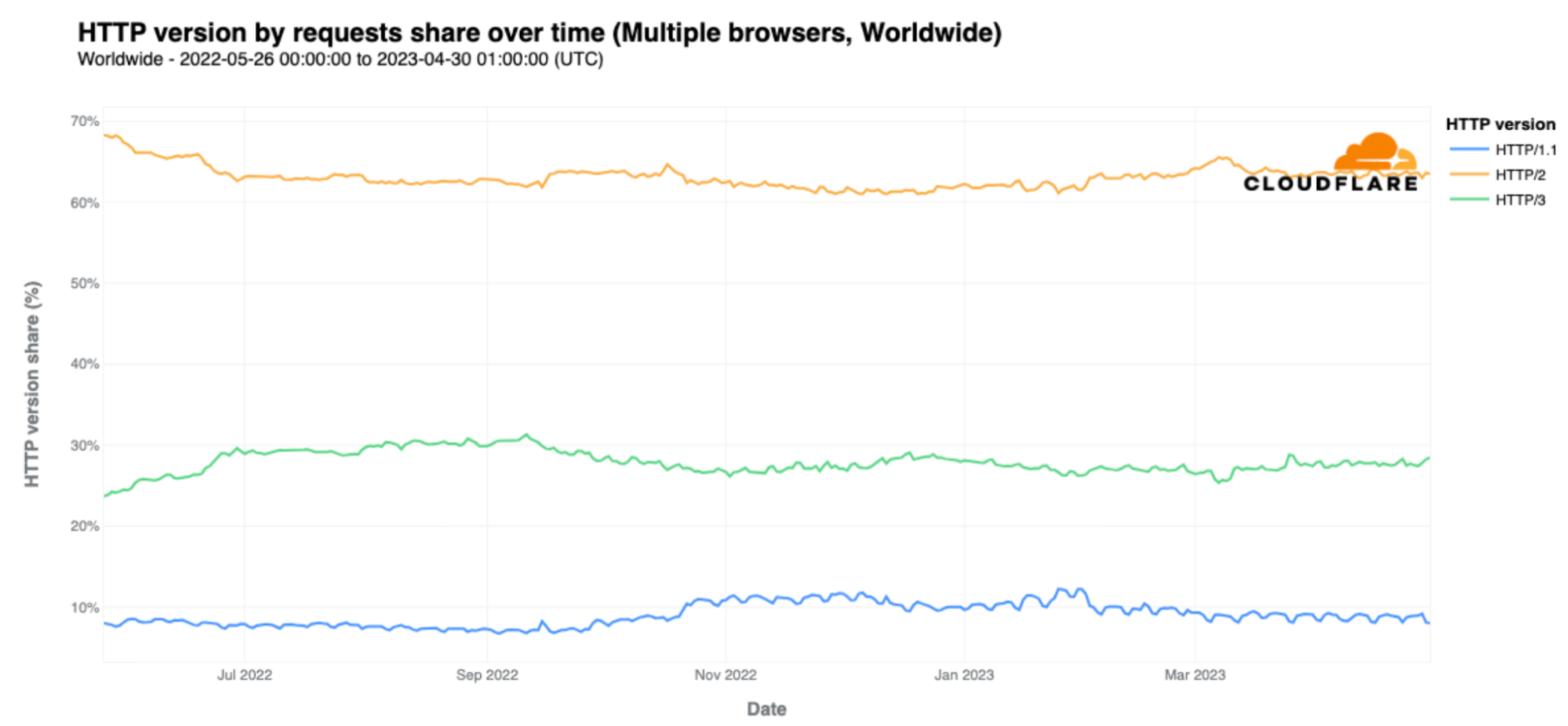
We’re excited about MASQUE because it fits into the way the Internet is evolving. According to this year’s usage report from our Radar team, HTTP/2 is currently the standard in use by the majority of Internet traffic, but HTTP/3 occupies a growing share – 28% as of June 2023. Cloudflare has always been dedicated towards adopting the cutting edge when it comes to standards: when RFC 9000 (the QUIC transport protocol) was published, we enabled it for all Cloudflare customers the very next day.

Donning a MASQUE: building a new protocol into Cloudflare WARP

So why do we think HTTP/3 is so promising? Well, a lot of it has to do with solving performance issues with HTTP/2. HTTP/3 promises a number of things.

Faster connection establishment: the TCP+TLS handshake of earlier HTTP versions typically takes two to three round trips. QUIC performs the transport and security handshake at the same time, cutting down on the total required round trips.

No more head of line blocking: when one packet of information does not make it to its destination, it will no longer block all streams of information.

Agility and evolution: QUIC has strong extension and version negotiation mechanisms. And because it encrypts all but a few bits of its wire image, deploying new transport features is easier and more practical. In contrast, TCP evolution was hampered by middleboxes that failed to keep up with the times.

Naturally, we’d want the proxying protocol we use for so many people’s everyday browsing to take advantage of these benefits. For example, the QUIC unreliable datagram extension doesn't help much for standard web traffic but it's ideal for tunneling UDP or IP packets that expect an unreliable substrate beneath them. Without the unreliable aspect, the protocols on top can get upset and start to perform badly. Datagrams help unlock QUIC's proxying potential.

MASQUE: A new era for VPN performance and flexibility

You may have heard of HTTP GET, POST, and PUT, but what about CONNECT? HTTP-CONNECT is a method that opens up a tunnel between servers and proxies traffic between them. For a deeper dive, check out our Primer on Proxies. Many Cloudflare services use this method like so:

Donning a MASQUE: building a new protocol into Cloudflare WARP

Clients send a CONNECT request, and if the proxy sends back a 2xx (success) status code, tunnel secured! Simple. However, remember that QUIC is UDP-based. Luckily, the MASQUE working group has figured out how to run multiple concurrently stream and datagram-based connections. Establishing one looks like this:

Donning a MASQUE: building a new protocol into Cloudflare WARP

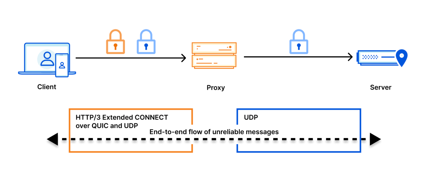
Here’s what this MASQUE proxying looks like:

Donning a MASQUE: building a new protocol into Cloudflare WARP

From a development perspective, MASQUE also allows us to improve our performance in other ways: we’re already running it for iCloud Private Relay and other Privacy Proxy partners. The services that power these partnerships, from our Rust-based proxy framework to our open source QUIC implementation, are already deployed globally in our network and have proven to be fast, resilient, and reliable. We've already learned a lot about how to operate proxies at scale, but there’s plenty of room for improvement. The good news is that every performance improvement we make to speed up MASQUE-based connections for our WARP clients will also improve performance for our customers that use HTTP-CONNECT, and vice-versa.

From a protocol perspective, we also think that MASQUE will prove to be resilient over time. As you can see above, connections are made through port 443, which for both TCP and UDP blends in well with general HTTP/3 traffic and is less susceptible than Wireguard to blocking.

Finally, because MASQUE is an IETF standard, innovations via extensions are already underway. One we’re particularly excited about is Multipath QUIC, an extension whose implementation would allow us to use multiple concurrent network interfaces for a single logical QUIC connection. For example, using both LTE and WiFi on a single mobile device could allow for seamless switching between the two, helping to avoid pesky disruptions when you’re coming to and from work or home.

The magic of supporting MASQUE is that it combines some pretty cool (and very Cloudflare-y!) elements: a standards-based proxying protocol that provides real user-facing performance benefits, built upon Cloudflare’s widely available Anycast network, and encryption of that last-mile between that network and your phone.

So how can I use it?

If you’d like to join the waitlist for our beta tester program for MASQUE, you can sign up here.

You’ll first need to download Testflight on a valid iOS device. We will be sending out invites to download the app via Testflight first come, first served, as early as next week. Once you’ve downloaded the app, MASQUE will be available as the default connection in our beta iOS version, only available in iOS 17 (and up).

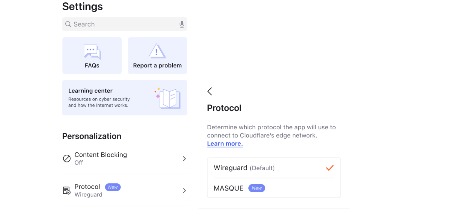
To toggle between Wireguard and MASQUE, go to Settings > Personalization > Protocol:

Donning a MASQUE: building a new protocol into Cloudflare WARP

Protocols come and go, but our privacy promise remains the same

While the protocols that dominate the Internet may change, our promise to consumers remains the same – a more private Internet, free of cost. When using WARP, we still route all DNS queries through 1.1.1.1, our privacy-respecting DNS resolver; we will never write user-identifiable log data to disk; we will never sell your browsing data or use it in any way to target you with advertising data; and you can still use WARP without providing any personal information like your name, phone number, or email address.

The Raspberry Pi Foundation and edX: A new way to learn about teaching computing

Post Syndicated from Ben Hall original https://www.raspberrypi.org/blog/the-raspberry-pi-foundation-and-edx-learn-about-teaching-computing/

We are delighted to announce that we’ve joined the partner network of edX, the global online learning platform. Through our free online courses we enable any educator to teach students about computing and how to create with digital technologies. Since 2017, over 250,000 people have taken our online courses, including 19,000 teachers in England alone. The move to edX builds on this success to help us bring high-quality training to many more teachers worldwide. 

“I feel that this course was essential in my understanding of where I may take my students on their journey as coders. Extremely practical advice and exercises.” – Online course participant

Free training to support all educators to teach computing

Supporting teachers and educators is crucial for our mission to enable young people to realise their full potential through the power of computing and digital technologies. Through our online courses educators can learn the skills, knowledge, and confidence to teach computing in an engaging way. As a result, they empower young people to in turn develop the knowledge, skills, and confidence to use digital technologies effectively, and to be able to critically evaluate these technologies and confidently engage with technological change.

Twenty of our most popular online courses are now available for sign-up on the edX platform. They will start in two blocks of ten in August and September, respectively. 

The courses are written with educators in mind, and are also useful to anyone with an interest in computing. The scope of topics is broad and includes programming in Python and Scratch, web development and design, cybersecurity, and machine learning and AI. Our aim is to support educators of all levels of experience to learn about computing, including teachers, club volunteers, youth workers, parents, and more. The courses also draw on content from our Computing Curriculum and provide support for teachers who want to engage their students with Experience AI, our pioneering education initiative about the field of AI.

“Our partnership with edX gives teachers everywhere a new way to engage with our free, expert-led computing education training. As people design and deploy new and powerful digital technologies, it’s important that no-one is left behind and we are all able to shape technology together.” – Sian Harris, Chief Education Officer at the Raspberry Pi Foundation

What are our courses like?

Designed, created, and facilitated by us, each of our courses is a cross-team project. When we put together a course we:

  • Use pedagogical best practice: we lead with concepts, model processes, and include activities that are ready for the classroom; add variety in terms of what content to present as text, images, or videos; and include opportunities to create projects
  • Use language carefully so that it is easy to follow for all participants, as are engaging with us online and may have English as an additional language
  • Put accessibility front and centre so that as many people as possible can learn with us

Offering our courses on the edX platform gives us flexibility in how we present the content, meaning we can better meet learner needs.

“Not only did the course present a thorough grounding in computing pedagogy, references were made to supporting research, and the structure and presentation was deceptively straightforward — despite dealing with some tricky concepts.” – Online course participant

We especially strive to exemplify the pedagogical approaches we recommend to teachers within the courses themselves. For example, semantic waves are woven throughout our learning resources and help learners to unpack new concepts, then repack them into more complex contexts to encourage knowledge acquisition. This teaching strategy, along with many others, is used widely in the courses and in all our teaching and learning resources.

How you can learn with us on edX

Taking our courses on edX you can:

  • Learn at your computer or on the edX mobile app
  • Join a course’s dedicated discussion are to discuss and collaborate with other participants
  • Ask our team questions — we’ll have experienced facilitators on hand

All the courses can be completed at your own pace, in your own time. Based on a commitment of between 1 to 2 hours per week, you can complete our courses in 2 to 4 weeks. You’re also welcome to work through them more quickly (or slowly) if you prefer.

Browse our selection of free courses and decide what your next learning adventure will be. 

We look forward to catching up with you in the course discussions on our new platform.

The post The Raspberry Pi Foundation and edX: A new way to learn about teaching computing appeared first on Raspberry Pi Foundation.

Да погледнем към Гърция

Post Syndicated from Александър Нуцов original https://www.toest.bg/da-poglednem-kum-gurtsiya/

Да погледнем към Гърция

На 21 май в Гърция се проведоха предсрочни парламентарни избори, спечелени убедително от дясноцентристката партия „Нова демокрация“ на Кириакос Мицотакис. След рулетката на мандатите за съставяне на правителство обаче такова не бе сформирано, а президентът насрочи нови избори за 25 юни. Какво и защо се случва в Гърция и влияе ли това на България? На тези въпроси ще потърсим отговор в следващите редове.

Преди изборите

На 22 април действащият тогава премиер Мицотакис официално поиска от президента Катерина Сакеларопулу да разпусне парламента и да насрочи нови избори. Формално четиригодишният мандат на правителството трябваше да изтече през юли, но според Мицотакис кабинетът бе изпълнил своята управленска програма предсрочно. Така по чл. 41 (ал. 2) от гръцката Конституция, във връзка с нуждата от разрешаване на национален въпрос от изключителна важност, парламентът беше разпуснат, а изборите се проведоха на 21 май 2023 г.

Конкретната тема от национално значение, изтъкната от Мицотакис, е свързана с усилията на Гърция да възвърне своя инвестиционен кредитен рейтинг в рамките на тази година. Такава заявка той направи още през януари, подчертавайки нуждата от провеждане на избори, които да осигурят политическа стабилност и дългосрочен мандат за управление.

Очакваше се Мицотакис да поиска нови избори още през април, но трагичната влакова катастрофа през февруари, отнела живота на 57 души, отложи намеренията на управляващите. Освен от натиска на последвалите протести срещу начина на управление на железопътния транспорт, майските избори бяха белязани от още няколко ключови събития.

През февруари гръцкият парламент забрани на партии, чиито ръководители са били осъждани, да участват в изборите. Така например най-популярната политическа партия в крайнодясното пространство „Златна зора“, обявена от съда през 2020 г. за криминална групировка по обвинения за извършени престъпления от омраза, беше възпряна да излъчи собствени кандидати. Правителството на Мицотакис беше подложено на продължителни атаки и заради скандала с подслушването на Никос Андрулакис – лидера на третата по големина парламентарна формация ПАСОК, както и на други високопоставени фигури и журналисти.

Демокрация по гръцки

Въпреки неблагоприятните обстоятелства и атаките от лявото, център-лявото и крайнодясното пространство „Нова демокрация“ драстично надмина очакванията на социологическите агенции и постигна повече от убедителна победа, получавайки 40,8% от гласовете (146 места в парламента) срещу само 20,1% за социалистите на Алексис Ципрас от СИРИЗА. На трето място с 11,5% се наредиха социалдемократите от ПАСОК, следвани от Комунистическата партия със 7,2% и дясната популистка формация „Гръцко решение“ с 4,5%. Анализатори отдават успеха на високия икономически ръст, възстановяването на страната след COVID кризата, понижаването на напрежението с Турция и цялостната стабилност по отношение на фискалната и икономическата политика.

Подобно на България, и Гърция се превърна в арена на остри политически и обществени сблъсъци през последните месеци. Въпреки това избирателната активност в южната ни съседка беше с над 20 процентни пункта по-висока, отколкото у нас (61,1% там срещу само 40,69% на последните избори тук). В сравнение с предходния парламентарен вот в Гърция през 2019 г., страната също бележи лек ръст – тогава избирателната активност възлизаше на 57,78%.

И макар сами по себе си тези числа да не са отлични за една добре функционираща демокрация, подобна избирателна активност изглежда като мираж за българската действителност. Основните причини за това са няколко. От една страна, съседите ни притежават по-солидна политическа и гражданска култура като част от богатото си демократично историческо наследство. От друга, изборите там произвеждат устойчиви парламентарни мнозинства и правителства, които (макар и не без перипетии и скандали) изпълняват своите мандати. Така в сравнение с българите гръцките граждани са много по-добре защитени от феномена „избирателна умора“ и чувството за безсмислие на изборния процес, неспособен да произведе устойчиво управление.

Най-важната разлика вероятно е тази, че гръцките партии и парламент отразяват много по-добре политическия спектър – от крайнолявото, през центъра, до крайнодясното, представлявайки широка палитра от обществени групи, които традиционно отъждествяват себе си с идеите на една или друга политически сила. Резултатът от вота през май и същността на парламентарно представените партии онагледяват това разнообразие. Поради конюнктурни специфики лявото и дясното в България се размиват, а вотът се опростява до протестен и непротестен, корупционен и антикорупционен, простатукво и антистатукво. Така партиите нямат дълбоки устои и лесно губят идентичността си при негативна за тях промяна на политическите обстоятелства, защото страдат от липса на идеи и визия, с които хората да се асоциират.

По обратния логически път може да обясним успеха на „Нова демокрация“. Център-дясната партия спечели кампанията с център-десни политики. Стъпвайки на идейните си начала, Мицотакис наблегна на постигнатите икономически успехи, намалените данъците върху доходите на бизнеса и физическите лица, по-ниската безработицата, ръста на чуждестранните инвестиции и балансираната бюджетна политика. Занапред той обеща допълнително орязване на данъците, повишаване на износа и по-високи заплати.

На този фон основните му конкуренти от СИРИЗА и ПАСОК (борещи се за сходен тип електорат в лявото пространство) наблегнаха на очерняща кампания срещу „Нова демокрация“, свързана със споменатите скандали. Те обаче не успяха да очертаят ясна политическа и икономическа визия като контрапункт на своите опоненти и претърпяха логичен изборен крах. И нито скандалите, нито трагичният железопътен инцидент, предизвикал гнева на десетки хиляди граждани, нито фактът, че цяло едно ново поколение от близо половин милион млади избиратели (традиционно привлечени от прогресивните идеи на лявото) за пръв път получиха право да гласуват, бяха в състояние да променят съдбата на безидейната опозиция. Събития, от които нашите политически сили определено могат да се поучат.

С ново изборно законодателство към нови избори

Само няколко мандата не достигнаха на „Нова демокрация“ да състави самостоятелно мнозинство в 300-местния гръцки парламент. След като и победителите, и победените отказаха да водят преговори за коалиционно управление, президентът насрочи нови избори за 25 юни и назначи служебно правителство начело с шефа на Сметната палата Йоанис Сармас.

Докато майските избори се проведоха по въведената от СИРИЗА през 2016 г. обикновена пропорционална система (подобна на тази в България), с изборите на 25 юни се завръща типичната за Гърция бонусна схема, възстановена от „Нова демокрация“ със законови поправки през 2020 г. Този модел доминира в Гърция през последните три десетилетия. При него мандатите се разпределят на пропорционален принцип, но с бонус за първата политическа сила под формата на допълнителен брой депутати.

Прагът за влизане в парламента остава 3%. При изборен резултат от над 25% победителят автоматично получава 20 допълнителни депутати – плюс един депутат за всеки половин процентен пункт над този резултат. Максималният брой допълнителни народни представители за първата политическа сила може да достигне 50. Това е и основната причина, поради която Мицотакис отказа да води преговори за коалиционно правителство и тласна страната към още едни избори, очаквайки да спечели стабилно мнозинство благодарение на бонусната система.

Бонусната схема не беше приложена на изборите през май поради конституционната поправка от 2019 г. Според нея промените в изборното законодателство влизат в сила не от следващите, а от по-следващите поред избори след тяхното приемане.

Българо-гръцките отношения

Със значителните промени в геополитическата обстановка през последните години отношенията между България и Гърция сякаш започнаха да процъфтяват. Още през лятото и есента на 2021 г., когато цените на енергоносителите започнаха да се покачват, двете страни осъзнаха необходимостта от по-тясно сътрудничество – най вече в сферата на енергетиката. Неслучайно един от приоритетите на коалиционния кабинет на Кирил Петков по това време беше да реабилитира и ускори строежа на газовия интерконектор между Стара Загора и Комотини, който се бавеше повече от десетилетие.

По този повод се проведоха множество двустранни срещи на най-високо равнище между премиерите Петков и Мицотакис, между енергийните министри, шефовете на газопреносните и газоразпределителните оператори и други високопоставени длъжностни лица. Проектът има стратегическо значение за енергийната сигурност на страната и вноса на евтин газ по договора с Азербайджан, особено след руската инвазия в Украйна и едностранното прекратяване на доставките от страна на „Газпром“.

В края на април 2022 г. започна и строежът на плаващия терминал за втечнен природен газ в Александруполис – ключов инфраструктурен проект за диверсификацията на газовите доставки в региона. В него България участва с дял от 20%, а първоначално запазеният от страната ни капацитет от 500 млн. куб.м газ на година беше удвоен до 1 млрд. куб.м годишно за период от десет години. Доставките за България трябва да започнат в началото на 2024 г., когато се очаква съоръжението да бъде пуснато в експлоатация.

В началото на тази година двете страни възродиха и позабравената идея за изграждане на петролен тръбопровод между Бургас и Александруполис. През февруари България и Гърция подписаха меморандум за сътрудничество, а по-късно съставиха и двустранна работна група. Целевият срок за завършване на проекта е краят на 2024 г., когато изтича дерогацията на България за внос на руски петрол по наложените на Русия европейски санкции. Освен това двете държави се споразумяха да складират гръцки газ в българското газохранилище в Чирен. Това се налага поради липсата на инфраструктура за съхранение в южната ни съседка, докато Европейският съюз изисква от страните членки да поддържат стратегически резерви в размер на 15% от годишното си потребление.

Както става ясно, през последните две години енергетиката измести по важност други традиционни сфери на сътрудничество между България и Гърция, каквито са туризмът и търговията. Това се дължи главно на нарастващата роля на енергетиката като част от националната сигурност на европейските държави след сътресенията с цените на енергоносителите, руската агресия в Украйна и използването на енергийните доставки като лост за изнудване и влияние. При тези обстоятелства и България, и Гърция имат интерес сътрудничеството им в енергетиката и други ключови сфери да продължи да се задълбочава независимо от състава на бъдещото управление в южната ни съседка.

Заглавно изображение: Смяна на караула пред гръцкия парламент в Атина. Източник: Canva

Вечният длъжник остава, въпреки новия закон за несъстоятелност на физическите лица. Кой може да се възползва от него на практика?

Post Syndicated from VassilKendov original http://kendov.com/debt_to_the_death/

Вечният длъжник остава, въпреки новия закон за несъстоятелност на физическите лица. Кой може да се възползва от него на практика?

Започвам направо

На какви условия трябва да отговаряте, за да се възползвате от този закон и какво можете да очаквате?

„Чл. 2. Законът не се прилага по отношение на физическите лица, които упражняват търговска дейност, стопанска дейност, занаят или свободна професия.”

За тези лица се прилагат разпоредбите на търговския закон. За тях в друг пост, за да не става сложно. Друг е въпросът, че това са най-реномираните професии и те реално не ползват процедури по фалит, камо ли път тази. Говорим за адвокати, архитекти, лекари, застрахователи, земеделски производители, търговци ЕТ, художници, артисти, попфолк тупалки и др…
Тоест, на практика тези хора отпадат от разпоредбите на този закон.
И понеже много знаещи и незнаещи ще се упражняват с мнения, тук ключовите думи са „НА ПРАКТИКА”. Защото на теория ще могат, но по стара традиция създаваме закони, които да са неприложими или да не си вършат работата. Та този закон е точно такъв. Той НА ПРАКТИКА няма да се прилага за посочените дейности!

За да се възползвате, трябва да отговаряте на определението – ДОБРОСЪВЕСТЕН!

Много обичам когато се дава определение за добросъвестност. Да знаете, че добросъвестността не е въпрост на съвест, а на юридическо определение. Ето по-точно какво е то:

„Добросъвестен е длъжникът, който поема задължения съобразно своето имуществено състояние и доходи и който със своите действия не уврежда умишлено или поради небрежност интересите на кредиторите си.

(2) Не се счита за добросъвестен длъжник, който:

  1. е осъден за злоупотреба на доверие, за престъпление срещу кредиторите или за престъпление срещу финансовата, данъчната или осигурителната системи, освен ако е реабилитиран;
  2. през последната година преди подаване на молбата за откриване на производството по несъстоятелност не е упражнявал трудова или стопанска дейност по занятие, която да е източник на доходи, независимо от начина на нейното възлагане и изпълнение и не търси активно работа;
  3. през последните 5 години преди подаване на молбата за откриване на производството по несъстоятелност не е извършил нарушение на задължение за деклариране на доходи или имущество;
  4. се е разпоредил безвъзмездно със свое имущество на значителна стойност през последните 5 години преди подаване на молбата за откриване на производство по несъстоятелност;
  5. през последните 5 години преди подаване на молбата за откриване на производство по несъстоятелност е поел задължение по договор за заем, договор за покупка на стоки и услуги или друг възмезден договор, който не е предназначен за задоволяване на негови или на членовете на семейството, които издържа, основни жизнени потребности и когато това задължение е явно несъобразено с имуществото и доходите му;
  6. е представил неверни или непълни данни, документи или доказателства за своето имущество пред съда или синдика във връзка с производство по несъстоятелност;
  7. не е оказал съдействие или е препятствал упражняването на правомощията на съда и на синдика относно проверката на имуществото му, опазването и попълването на масата на несъстоятелността;
  8. не е изпълнил задължения, предвидени в този закон, в одобрен погасителен план или в извънсъдебно споразумение с кредиторите, с което е създал опасност за интересите на кредиторите.

(3) Значителна стойност на имуществото по ал. 2, т. 4 е стойност, която надхвърля средния месечен доход на длъжника за последните 12 месеца, определена към момента на разпореждането.

(4) Явно несъобразено с имуществото и доходите на длъжника е задължение, чието изпълнение, самостоятелно или в съвкупност с други задължения на длъжника, е несъвместимо с разходите за задоволяване на жизнените потребности на длъжника и на членовете на неговото семейство, на които той дължи издръжка. При преценката на обстоятелствата по ал. 2, т. 5 се вземат предвид всички задължения на длъжника, както и имуществото и доходите на длъжника към момента на поемане на задължението.”

Аз не мисля, че има смисъл да коментирам горното, но мога да се закълна в 2 неща:

За  срещa с мен моля използвайте посочената форма.

[contact-form-7]

1. Това определение отхвърли възможността на 99% от хората да се възползват от тази процедура.

2. На останалия 1% от хората, ще им се отще да плащат адвокатски хонорари през следващите 3-4 години, само докато се докаже дали те са добросъвестни или не.

За да не разводняваме по-нататък анализа, искам да Ви обърна внимание на чл. 15, в който се казва, че ако се окаже, че сте подали молба, а не е трябвало, защото не отговаряте на горните определения освен сумата, която очевидно не можете да плащате, дължите и обезщетение на кредиторите.
Това винаги ми е било любимото когато изпаднеш в просрочие по банков кредит. Ти не можеш да погасяваш редовната главница и лихвите, но те ти начисляват допълнително такси, ЧСИ разноски и наказателни лихви, за да може дългът ти да нарастне още повече.

За финал, ето и текста на чл. 15 от новивия закон:

„Чл. 15. (1) Длъжник, който подаде молба за откриване на производство по несъстоятелност, като знае, че няма основание за това, дължи обезщетение на кредиторите за претърпените във връзка с производството имуществени и неимуществени вреди, които са пряка и непосредствена последица от увреждането.

(2) Отговорността за заплащане на обезщетение по ал. 1 възниква, в случай че молбата на длъжника за откриване на производство по несъстоятелност е отхвърлена или образуваното производство по несъстоятелност е прекратено с влязло в сила решение поради недобросъвестност на длъжника.”

СИНДИКЪТ – новият душманин в закона за фалита на физическите лица

И ако сте стигнали до тук да знаете, че предварителната консултация е несравнимо по-евтина от бъдещите разходи и разправии

Васил Кендов – финансов съветник

За  срещa с мен моля използвайте посочената форма.

[contact-form-7]

The post Вечният длъжник остава, въпреки новия закон за несъстоятелност на физическите лица. Кой може да се възползва от него на практика? appeared first on Kendov.com.

Amazon OpenSearch Service’s vector database capabilities explained

Post Syndicated from Jon Handler original https://aws.amazon.com/blogs/big-data/amazon-opensearch-services-vector-database-capabilities-explained/

OpenSearch is a scalable, flexible, and extensible open-source software suite for search, analytics, security monitoring, and observability applications, licensed under the Apache 2.0 license. It comprises a search engine, OpenSearch, which delivers low-latency search and aggregations, OpenSearch Dashboards, a visualization and dashboarding tool, and a suite of plugins that provide advanced capabilities like alerting, fine-grained access control, observability, security monitoring, and vector storage and processing. Amazon OpenSearch Service is a fully managed service that makes it simple to deploy, scale, and operate OpenSearch in the AWS Cloud.

As an end-user, when you use OpenSearch’s search capabilities, you generally have a goal in mind—something you want to accomplish. Along the way, you use OpenSearch to gather information in support of achieving that goal (or maybe the information is the original goal). We’ve all become used to the “search box” interface, where you type some words, and the search engine brings back results based on word-to-word matching. Let’s say you want to buy a couch in order to spend cozy evenings with your family around the fire. You go to Amazon.com, and you type “a cozy place to sit by the fire.” Unfortunately, if you run that search on Amazon.com, you get items like fire pits, heating fans, and home decorations—not what you intended. The problem is that couch manufacturers probably didn’t use the words “cozy,” “place,” “sit,” and “fire” in their product titles or descriptions.

In recent years, machine learning (ML) techniques have become increasingly popular to enhance search. Among them are the use of embedding models, a type of model that can encode a large body of data into an n-dimensional space where each entity is encoded into a vector, a data point in that space, and organized such that similar entities are closer together. An embedding model, for instance, could encode the semantics of a corpus. By searching for the vectors nearest to an encoded document — k-nearest neighbor (k-NN) search — you can find the most semantically similar documents. Sophisticated embedding models can support multiple modalities, for instance, encoding the image and text of a product catalog and enabling similarity matching on both modalities.

A vector database provides efficient vector similarity search by providing specialized indexes like k-NN indexes. It also provides other database functionality like managing vector data alongside other data types, workload management, access control and more. OpenSearch’s k-NN plugin provides core vector database functionality for OpenSearch, so when your customer searches for “a cozy place to sit by the fire” in your catalog, you can encode that prompt and use OpenSearch to perform a nearest neighbor query to surface that 8-foot, blue couch with designer arranged photographs in front of fireplaces.

Using OpenSearch Service as a vector database

With OpenSearch Service’s vector database capabilities, you can implement semantic search, Retrieval Augmented Generation (RAG) with LLMs, recommendation engines, and search rich media.

Semantic search

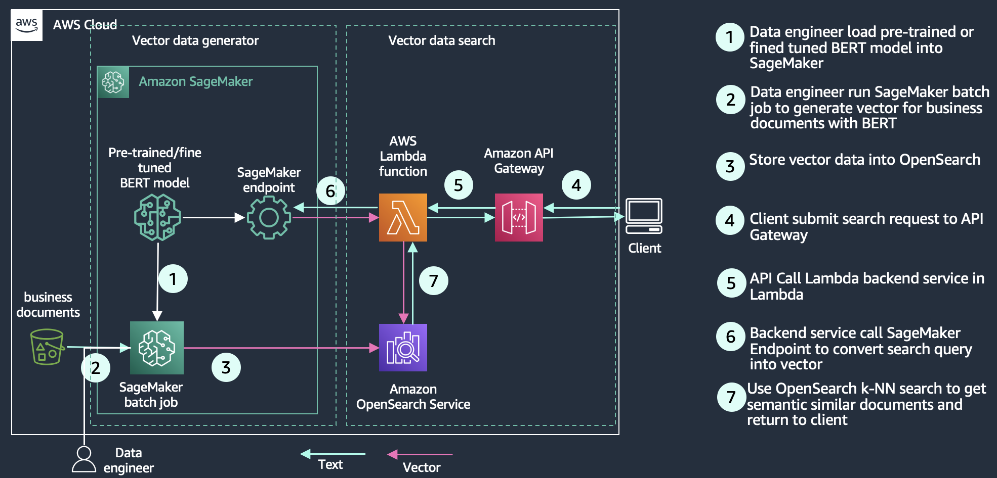
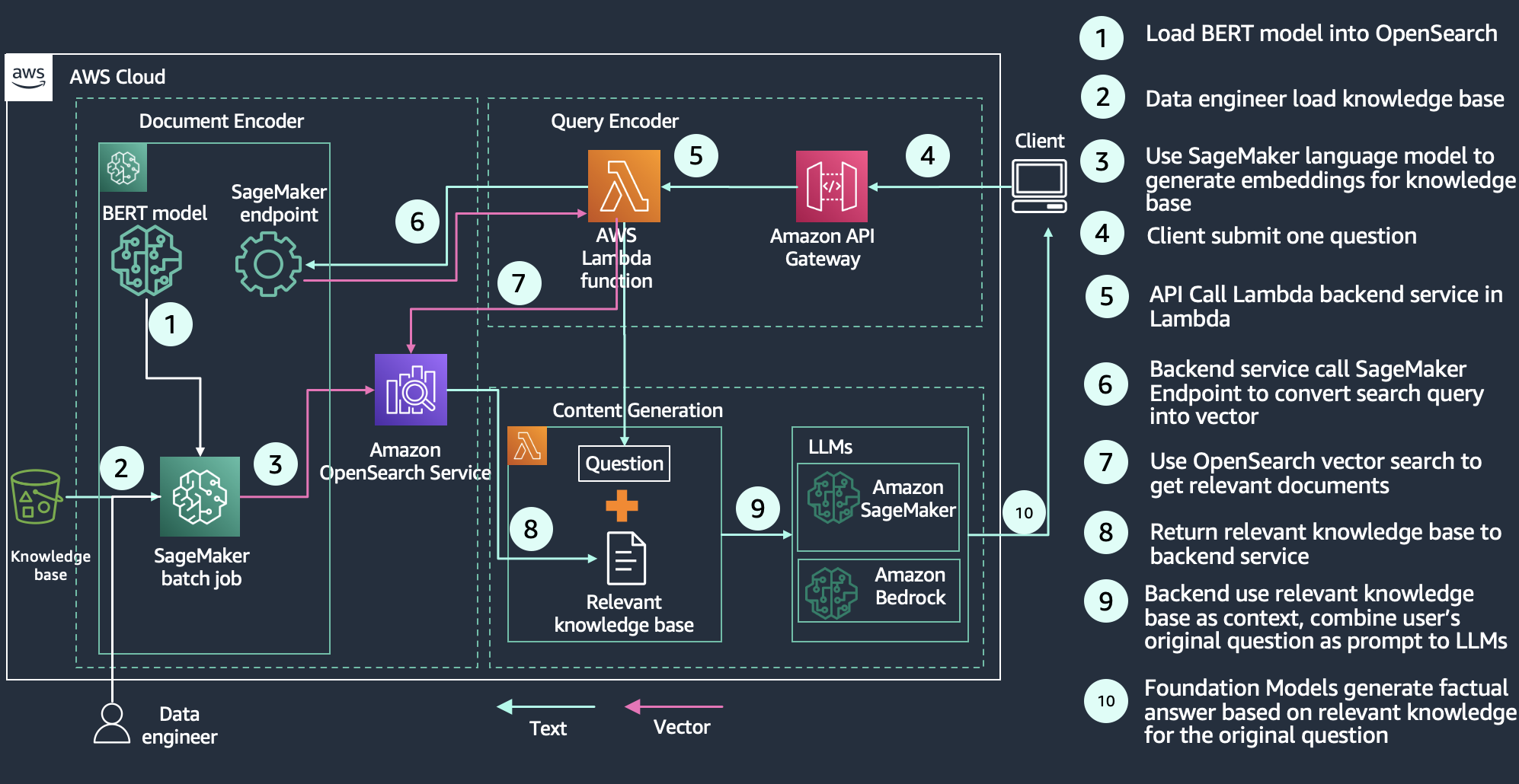
With semantic search, you improve the relevance of retrieved results using language-based embeddings on search documents. You enable your search customers to use natural language queries, like “a cozy place to sit by the fire” to find their 8-foot-long blue couch. For more information, refer to Building a semantic search engine in OpenSearch to learn how semantic search can deliver a 15% relevance improvement, as measured by normalized discounted cumulative gain (nDCG) metrics compared with keyword search. For a concrete example, our Improve search relevance with ML in Amazon OpenSearch Service workshop explores the difference between keyword and semantic search, based on a Bidirectional Encoder Representations from Transformers (BERT) model, hosted by Amazon SageMaker to generate vectors and store them in OpenSearch. The workshop uses product question answers as an example to show how keyword search using the keywords/phrases of the query leads to some irrelevant results. Semantic search is able to retrieve more relevant documents by matching the context and semantics of the query. The following diagram shows an example architecture for a semantic search application with OpenSearch Service as the vector database.

Architecture diagram showing how to use Amazon OpenSearch Service to perform semantic search to improve relevance

Retrieval Augmented Generation with LLMs

RAG is a method for building trustworthy generative AI chatbots using generative LLMs like OpenAI, ChatGPT, or Amazon Titan Text. With the rise of generative LLMs, application developers are looking for ways to take advantage of this innovative technology. One popular use case involves delivering conversational experiences through intelligent agents. Perhaps you’re a software provider with knowledge bases for product information, customer self-service, or industry domain knowledge like tax reporting rules or medical information about diseases and treatments. A conversational search experience provides an intuitive interface for users to sift through information through dialog and Q&A. Generative LLMs on their own are prone to hallucinations—a situation where the model generates a believable but factually incorrect response. RAG solves this problem by complementing generative LLMs with an external knowledge base that is typically built using a vector database hydrated with vector-encoded knowledge articles.

As illustrated in the following diagram, the query workflow starts with a question that is encoded and used to retrieve relevant knowledge articles from the vector database. Those results are sent to the generative LLM whose job is to augment those results, typically by summarizing the results as a conversational response. By complementing the generative model with a knowledge base, RAG grounds the model on facts to minimize hallucinations. You can learn more about building a RAG solution in the Retrieval Augmented Generation module of our semantic search workshop.

Architecture diagram showing how to use Amazon OpenSearch Service to perform retrieval-augmented generation

Recommendation engine

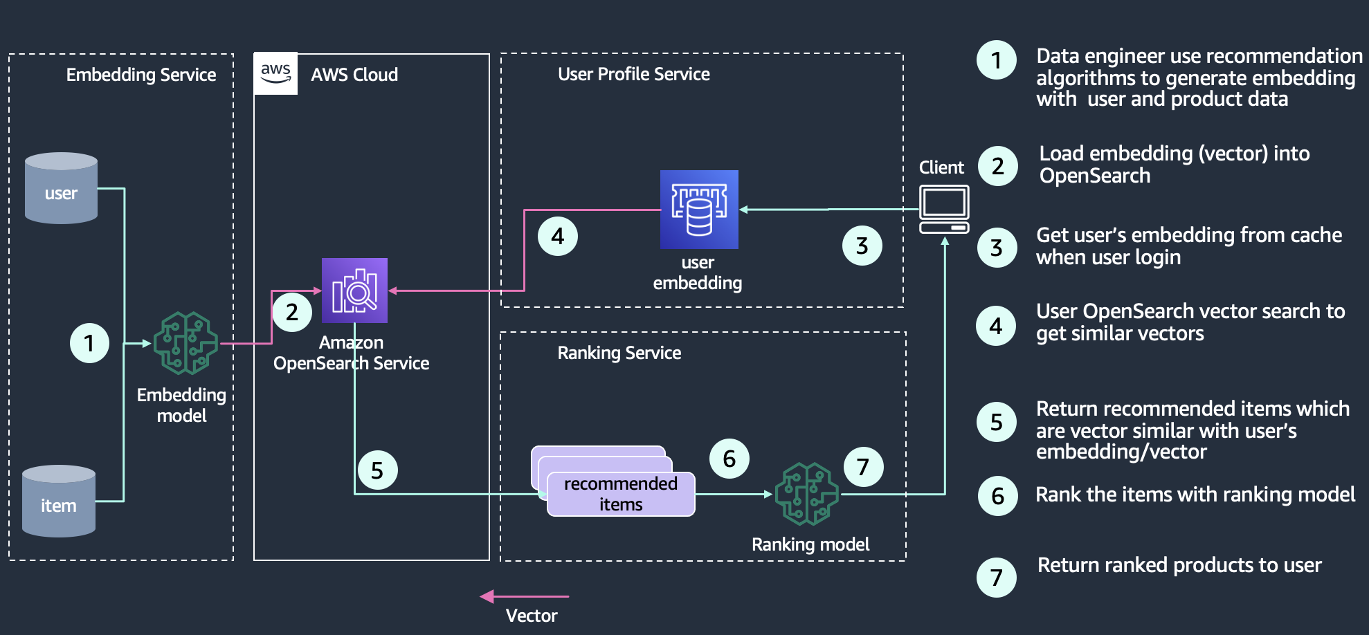
Recommendations are a common component in the search experience, especially for ecommerce applications. Adding a user experience feature like “more like this” or “customers who bought this also bought that” can drive additional revenue through getting customers what they want. Search architects employ many techniques and technologies to build recommendations, including Deep Neural Network (DNN) based recommendation algorithms such as the two-tower neural net model, YoutubeDNN. A trained embedding model encodes products, for example, into an embedding space where products that are frequently bought together are considered more similar, and therefore are represented as data points that are closer together in the embedding space. Another possibility
is that product embeddings are based on co-rating similarity instead of purchase activity. You can employ this affinity data through calculating the vector similarity between a particular user’s embedding and vectors in the database to return recommended items. The following diagram shows an example architecture of building a recommendation engine with OpenSearch as a vector store.

Architecture diagram showing how to use Amazon OpenSearch Service as a recommendation engine

Media search

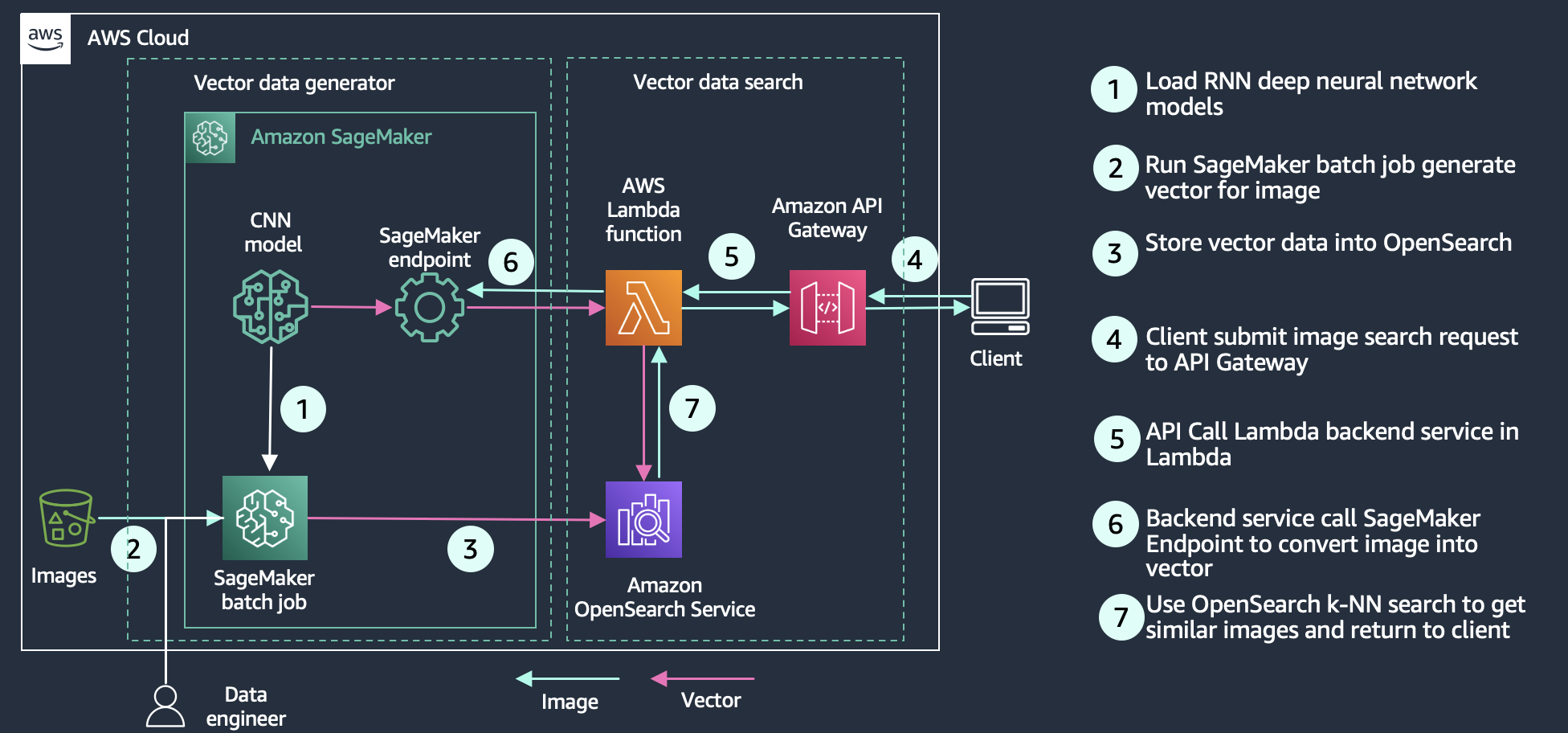
Media search enables users to query the search engine with rich media like images, audio, and video. Its implementation is similar to semantic search—you create vector embeddings for your search documents and then query OpenSearch Service with a vector. The difference is you use a computer vision deep neural network (e.g. Convolutional Neural Network (CNN)) such as ResNet to convert images into vectors. The following diagram shows an example architecture of building an image search with OpenSearch as the vector store.

Architecture diagram showing how to use Amazon OpenSearch Service to search rich media like images, videos, and audio files

Understanding the technology

OpenSearch uses approximate nearest neighbor (ANN) algorithms from the NMSLIB, FAISS, and Lucene libraries to power k-NN search. These search methods employ ANN to improve search latency for large datasets. Of the three search methods the k-NN plugin provides, this method offers the best search scalability for large datasets. The engine details are as follows:

  • Non-Metric Space Library (NMSLIB) – NMSLIB implements the HNSW ANN algorithm
  • Facebook AI Similarity Search (FAISS) – FAISS implements both HNSW and IVF ANN algorithms
  • Lucene – Lucene implements the HNSW algorithm

Each of the three engines used for approximate k-NN search has its own attributes that make one more sensible to use than the others in a given situation. You can follow the general information in this section to help determine which engine will best meet your requirements.

In general, NMSLIB and FAISS should be selected for large-scale use cases. Lucene is a good option for smaller deployments, but offers benefits like smart filtering where the optimal filtering strategy—pre-filtering, post-filtering, or exact k-NN—is automatically applied depending on the situation. The following table summarizes the differences between each option.

.

NMSLIB-HNSW

FAISS-HNSW

FAISS-IVF

Lucene-HNSW

Max Dimension

16,000

16,000

16,000

1024

Filter

Post filter

Post filter

Post filter

Filter while search

Training Required

No

No

Yes

No

Similarity Metrics

l2, innerproduct, cosinesimil, l1, linf

l2, innerproduct

l2, innerproduct

l2, cosinesimil

Vector Volume

Tens of billions

Tens of billions

Tens of billions

< Ten million

Indexing latency

Low

Low

Lowest

Low

Query Latency & Quality

Low latency & high quality

Low latency & high quality

Low latency & low quality

High latency & high quality

Vector Compression

Flat

Flat

Product Quantization

Flat

Product Quantization

Flat

Memory Consumption

High

High

Low with PQ

Medium

Low with PQ

High

Approximate and exact nearest-neighbor search

The OpenSearch Service k-NN plugin supports three different methods for obtaining the k-nearest neighbors from an index of vectors: approximate k-NN, score script (exact k-NN), and painless extensions (exact k-NN).

Approximate k-NN

The first method takes an approximate nearest neighbor approach—it uses one of several algorithms to return the approximate k-nearest neighbors to a query vector. Usually, these algorithms sacrifice indexing speed and search accuracy in return for performance benefits such as lower latency, smaller memory footprints, and more scalable search. Approximate k-NN is the best choice for searches over large indexes (that is, hundreds of thousands of vectors or more) that require low latency. You should not use approximate k-NN if you want to apply a filter on the index before the k-NN search, which greatly reduces the number of vectors to be searched. In this case, you should use either the score script method or painless extensions.

Score script

The second method extends the OpenSearch Service score script functionality to run a brute force, exact k-NN search over knn_vector fields or fields that can represent binary objects. With this approach, you can run k-NN search on a subset of vectors in your index (sometimes referred to as a pre-filter search). This approach is preferred for searches over smaller bodies of documents or when a pre-filter is needed. Using this approach on large indexes may lead to high latencies.

Painless extensions

The third method adds the distance functions as painless extensions that you can use in more complex combinations. Similar to the k-NN score script, you can use this method to perform a brute force, exact k-NN search across an index, which also supports pre-filtering. This approach has slightly slower query performance compared to the k-NN score script. If your use case requires more customization over the final score, you should use this approach over score script k-NN.

Vector search algorithms

The simple way to find similar vectors is to use k-nearest neighbors (k-NN) algorithms, which compute the distance between a query vector and the other vectors in the vector database. As we mentioned earlier, the score script k-NN and painless extensions search methods use the exact k-NN algorithms under the hood. However, in the case of extremely large datasets with high dimensionality, this creates a scaling problem that reduces the efficiency of the search. Approximate nearest neighbor (ANN) search methods can overcome this by employing tools that restructure indexes more efficiently and reduce the dimensionality of searchable vectors. There are different ANN search algorithms; for example, locality sensitive hashing, tree-based, cluster-based, and graph-based. OpenSearch implements two ANN algorithms: Hierarchical Navigable Small Worlds (HNSW) and Inverted File System (IVF). For a more detailed explanation of how the HNSW and IVF algorithms work in OpenSearch, see blog post “Choose the k-NN algorithm for your billion-scale use case with OpenSearch”.

Hierarchical Navigable Small Worlds

The HNSW algorithm is one of the most popular algorithms out there for ANN search. The core idea of the algorithm is to build a graph with edges connecting index vectors that are close to each other. Then, on search, this graph is partially traversed to find the approximate nearest neighbors to the query vector. To steer the traversal towards the query’s nearest neighbors, the algorithm always visits the closest candidate to the query vector next.

Inverted File

The IVF algorithm separates your index vectors into a set of buckets, then, to reduce your search time, only searches through a subset of these buckets. However, if the algorithm just randomly split up your vectors into different buckets, and only searched a subset of them, it would yield a poor approximation. The IVF algorithm uses a more elegant approach. First, before indexing begins, it assigns each bucket a representative vector. When a vector is indexed, it gets added to the bucket that has the closest representative vector. This way, vectors that are closer to each other are placed roughly in the same or nearby buckets.

Vector similarity metrics

All search engines use a similarity metric to rank and sort results and bring the most relevant results to the top. When you use a plain text query, the similarity metric is called TF-IDF, which measures the importance of the terms in the query and generates a score based on the number of textual matches. When your query includes a vector, the similarity metrics are spatial in nature, taking advantage of proximity in the vector space. OpenSearch supports several similarity or distance measures:

  • Euclidean distance – The straight-line distance between points.
  • L1 (Manhattan) distance – The sum of the differences of all of the vector components. L1 distance measures how many orthogonal city blocks you need to traverse from point A to point B.
  • L-infinity (chessboard) distance – The number of moves a King would make on an n-dimensional chessboard. It’s different than Euclidean distance on the diagonals—a diagonal step on a 2-dimensional chessboard is 1.41 Euclidean units away, but 2 L-infinity units away.
  • Inner product – The product of the magnitudes of two vectors and the cosine of the angle between them. Usually used for natural language processing (NLP) vector similarity.
  • Cosine similarity – The cosine of the angle between two vectors in a vector space.
  • Hamming distance – For binary-coded vectors, the number of bits that differ between the two vectors.

Advantage of OpenSearch as a vector database

When you use OpenSearch Service as a vector database, you can take advantage of the service’s features like usability, scalability, availability, interoperability, and security. More importantly, you can use OpenSearch’s search features to enhance the search experience. For example, you can use Learning to Rank in OpenSearch to integrate user clickthrough behavior data into your search application and improve search relevance. You can also combine OpenSearch text search and vector search capabilities to search documents with keyword and semantic similarity. You can also use other fields in the index to filter documents to improve relevance. For advanced users, you can use a hybrid scoring model to combine OpenSearch’s text-based relevance score, computed with the Okapi BM25 function and its vector search score to improve the ranking of your search results.

Scale and limits

OpenSearch as vector database support billions of vector records. Keep in mind the following calculator regarding number of vectors and dimensions to size your cluster.

Number of vectors

OpenSearch VectorDB takes advantage of the sharding capabilities of OpenSearch and can scale to billions of vectors at single-digit millisecond latencies by sharding vectors and scale horizontally by adding more nodes. The number of vectors that can fit in a single machine is a function of the off-heap memory availability on the machine. The number of nodes required will depend on the amount of memory that can be used for the algorithm per node and the total amount of memory required by the algorithm. The more nodes, the more memory and better performance. The amount of memory available per node is computed as memory_available = (node_memory – jvm_size) * circuit_breaker_limit, with the following parameters:

  • node_memory – The total memory of the instance.
  • jvm_size – The OpenSearch JVM heap size. This is set to half of the instance’s RAM, capped at approximately 32 GB.
  • circuit_breaker_limit – The native memory usage threshold for the circuit breaker. This is set to 0.5.

Total cluster memory estimation depends on total number of vector records and algorithms. HNSW and IVF have different memory requirements. You can refer to Memory Estimation for more details.

Number of dimensions

OpenSearch’s current dimension limit for the vector field knn_vector is 16,000 dimensions. Each dimension is represented as a 32-bit float. The more dimensions, the more memory you’ll need to index and search. The number of dimensions is usually determined by the embedding models that translate the entity to a vector. There are a lot of options to choose from when building your knn_vector field. To determine the correct methods and parameters to choose, refer to Choosing the right method.

Customer stories:

Amazon Music

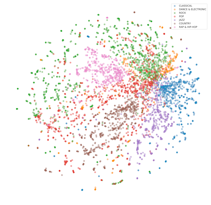
Amazon Music is always innovating to provide customers with unique and personalized experiences. One of Amazon Music’s approaches to music recommendations is a remix of a classic Amazon innovation, item-to-item collaborative filtering, and vector databases. Using data aggregated based on user listening behavior, Amazon Music has created an embedding model that encodes music tracks and customer representations into a vector space where neighboring vectors represent tracks that are similar. 100 million songs are encoded into vectors, indexed into OpenSearch, and served across multiple geographies to power real-time recommendations. OpenSearch currently manages 1.05 billion vectors and supports a peak load of 7,100 vector queries per second to power Amazon Music recommendations.

The item-to-item collaborative filter continues to be among the most popular methods for online product recommendations because of its effectiveness at scaling to large customer bases and product catalogs. OpenSearch makes it easier to operationalize and further the scalability of the recommender by providing scale-out infrastructure and k-NN indexes that grow linearly with respect to the number of tracks and similarity search in logarithmic time.

The following figure visualizes the high-dimensional space created by the vector embedding.

A visualization of the vector encoding of Amazon Music entries in the large vector space

Brand protection at Amazon

Amazon strives to deliver the world’s most trustworthy shopping experience, offering customers the widest possible selection of authentic products. To earn and maintain our customers’ trust, we strictly prohibit the sale of counterfeit products, and we continue to invest in innovations that ensure only authentic products reach our customers. Amazon’s brand protection programs build trust with brands by accurately representing and completely protecting their brand. We strive to ensure that public perception mirrors the trustworthy experience we deliver. Our brand protection strategy focuses on four pillars: (1) Proactive Controls (2) Powerful Tools to Protect Brands (3) Holding Bad Actors Accountable (4) Protecting and Educating Customers. Amazon OpenSearch Service is a key part of Amazon’s Proactive Controls.

In 2022, Amazon’s automated technology scanned more than 8 billion attempted changes daily to product detail pages for signs of potential abuse. Our proactive controls found more than 99% of blocked or removed listings before a brand ever had to find and report it. These listings were suspected of being fraudulent, infringing, counterfeit, or at risk of other forms of abuse. To perform these scans, Amazon created tooling that uses advanced and innovative techniques, including the use of advanced machine learning models to automate the detection of intellectual property infringements in listings across Amazon’s stores globally. A key technical challenge in implementing such automated system is the ability to search for protected intellectual property within a vast billion-vector corpus in a fast, scalable and cost effective manner. Leveraging Amazon OpenSearch Service’s scalable vector database capabilities and distributed architecture, we successfully developed an ingestion pipeline that has indexed a total of 68 billion, 128- and 1024-dimension vectors into OpenSearch Service to enable brands and automated systems to conduct infringement detection, in real-time, through a highly available and fast (sub-second) search API.

Conclusion

Whether you’re building a generative AI solution, searching rich media and audio, or bringing more semantic search to your existing search-based application, OpenSearch is a capable vector database. OpenSearch supports a variety of engines, algorithms, and distance measures that you can employ to build the right solution. OpenSearch provides a scalable engine that can support vector search at low latency and up to billions of vectors. With OpenSearch and its vector DB capabilities, your users can find that 8-foot-blue couch easily, and relax by a cozy fire.


About the Authors

Jon Handler is a Senior Principal Solutions Architect with AWSJon Handler is a Senior Principal Solutions Architect at Amazon Web Services based in Palo Alto, CA. Jon works closely with OpenSearch and Amazon OpenSearch Service, providing help and guidance to a broad range of customers who have search and log analytics workloads that they want to move to the AWS Cloud. Prior to joining AWS, Jon’s career as a software developer included four years of coding a large-scale, eCommerce search engine. Jon holds a Bachelor of the Arts from the University of Pennsylvania, and a Master of Science and a Ph. D. in Computer Science and Artificial Intelligence from Northwestern University.

Jianwei Li is a Principal Analytics Specialist TAM at Amazon Web Services. Jianwei provides consultant service for customers to help customer design and build modern data platform. Jianwei has been working in big data domain as software developer, consultant and tech leader.

Dylan Tong is a Senior Product Manager at AWS. He works with customers to help drive their success on the AWS platform through thought leadership and guidance on designing well architected solutions. He has spent most of his career building on his expertise in data management and analytics by working for leaders and innovators in the space.

Vamshi Vijay Nakkirtha is a Software Engineering Manager working on the OpenSearch Project and Amazon OpenSearch Service. His primary interests include distributed systems. He is an active contributor to various plugins, like k-NN, GeoSpatial, and dashboard-maps.

Let’s Architect! Open-source technologies on AWS

Post Syndicated from Vittorio Denti original https://aws.amazon.com/blogs/architecture/lets-architect-open-source-technologies-on-aws/

We brought you a Let’s Architect! blog post about open-source on AWS that covered some technologies with development led by AWS/Amazon, as well as well-known solutions available on managed AWS services. Today, we’re following the same approach to share more insights about the process itself for developing open-source. That’s why the first topic we discuss in this post is a re:Invent talk from Heitor Lessa, Principal Solutions Architect at AWS, explaining some interesting approaches for developing and scaling successful open-source projects.

This edition of Let’s Architect! also touches on observability with Open Telemetry, Apache Kafka on AWS, and Infrastructure as Code with an hands-on workshop on AWS Cloud Development Kit (AWS CDK).

Powertools for AWS Lambda: Lessons from the road to 10 million downloads

Powertools for AWS Lambda is an open-source library to help engineering teams implement serverless best practices. In two years, Powertools went from an initial prototype to a fast-growing project in the open-source world. Rapid growth along with support from a wide community led to challenges from balancing new features with operational excellence to triaging bug reports and RFCs and scaling and redesigning documentation.

In this session, you can learn about Powertools for AWS Lambda to understand what it is and the problems it solves. Moreover, there are many valuable lessons to learn how to create and scale a successful open-source project. From managing the trade-off between releasing new features and achieving operational stability to measuring the impact of the project, there are many challenges in open-source projects that require careful thought.

Take me to this video!

Heitor Lessa describing one the key lessons: development and releasing new features should be as important as the other activities (governance, operational excellence, and more)

Heitor Lessa describing one of the key lessons: development and releasing new features should be as important as the other activities (governance, operational excellence, and more).

Observability the open-source way

The recent blog post Let’s Architect! Monitoring production systems at scale talks about the importance of monitoring. Setting up observability is critical to maintain application and infrastructure health, but instrumenting applications to collect monitoring signals such as metrics and logs can be challenging when using vendor-specific SDKs.

This video introduces you to OpenTelemetry, an open-source observability framework. OpenTelemetry provides a flexible, single vendor-agnostic SDK based on open-source specifications that developers can use to instrument and collect signals from applications. This resource explains how it works in practice and how to monitor microservice-based applications with the OpenTelemetry SDK.

Take me to this video!

With AWS Distro for OpenTelemetry, you can collect data from your AWS resources.

With AWS Distro for OpenTelemetry, you can collect data from your AWS resources.

Best practices for right-sizing your Apache Kafka clusters to optimize performance and cost

Apache Kafka is an open-source streaming data store that decouples applications producing streaming data (producers) into its data store from applications consuming streaming data (consumers) from its data store. Amazon Managed Streaming for Apache Kafka (Amazon MSK) allows you to use the open-source version of Apache Kafka with the service managing infrastructure and operations for you.

This blog post explains how the underlying infrastructure configuration can affect Apache Kafka performance. You can learn strategies on how to size the clusters to meet the desired throughput, availability, and latency requirements. This resource helps you discover strategies to find the optimal sizing for your resources, and learn the mental models adopted to conduct the investigation and derive the conclusions.

Take me to this blog!

Comparisons of put latencies for three clusters with different broker sizes

Comparisons of put latencies for three clusters with different broker sizes

AWS Cloud Development Kit workshop

AWS Cloud Development Kit (AWS CDK) is an open-source software development framework that allows you to provision cloud resources programmatically (Infrastructure as Code or IaC) by using familiar programming languages such as Python, Typescript, Javascript, Java, Go, and C#/.Net.

CDK allows you to create reusable template and assets, test your infrastructure, make deployments repeatable, and make your cloud environment stable by removing manual (and error-prone) operations. This workshop introduces you to CDK, where you can learn how to provision an initial simple application as well as become familiar with more advanced concepts like CDK constructs.

Take me to this workshop!

This construct can be attached to any Lambda function that is used as an API Gateway backend. It counts how many requests were issued to each URL.

This construct can be attached to any Lambda function that is used as an API Gateway backend. It counts how many requests were issued to each URL.

See you next time!

Thanks for joining our conversation! To find all the blogs from this series, you can check out the Let’s Architect! list of content on the AWS Architecture Blog.

Amazon SES – How to track email deliverability to domain level with CloudWatch

Post Syndicated from Alaa Hammad original https://aws.amazon.com/blogs/messaging-and-targeting/amazon-ses-how-to-track-email-deliverability-to-domain-level-with-cloudwatch/

Why is it important to track email deliverability per domain with Amazon Simple Email Service (SES)?

Amazon Simple Email Service (Amazon SES) is a scalable cloud email service provider that enables businesses to build a large-scale email solution and host multiple domains from the same SES account for different purposes ex: one domain for sending marketing emails such as special offers, another domain to send transactional emails such as order confirmations, and other types of correspondence such as newsletters.

As your product, service or solution built on Amazon SES grows and you require multiple domains verified, it is important to track email deliverability for emails you send from each domain for business continuity, billing purposes or incidents investigations. This can be useful to identify if you have low email deliverability for your business domain or if you have a domain generating high bounce or complaint rates and take proactive actions before impacting the account’s ability to send emails from any other domains.

SES offers features that automatically manage deliverability per domain through Virtual Deliverability Manager. Virtual Deliverability Manager helps enhance email deliverability and provides insights into sending and delivery data, as well as offering solutions to fix negative email sending reputation. You can learn more about Virtual Deliverability Manager here.

Solution Walkthrough

Amazon SES provides a way to monitor sender reputation metrics such as bounce and complaint rates per account or configuration sets using event publishing. This blog will discuss how you can use Amazon SES message auto-tags to monitor and publish email deliverability events (Send, Delivery, Bounce, Complaints) to CloudWatch custom metrics per domain. In addition, you will see how to create a custom CloudWatch dashboard that’s easy to access in a single view to monitor your domain metrics. This CloudWatch dashboard can help to provide guidance for your team members during operational events about how to respond to specific incidents for your sending domain.

What are Amazon SES Auto-Tags:

Message tags are a form of name/value pairs to categorize the email you are sending. For example, if you advertise books, you could name a message tag general, and assign a value of sci-fi or western, when you send an email for the associated campaign. Depending on which email sending interface you use, you can provide the message tag as a parameter to the API call (SendEmail, SendRawEmail) or as an Amazon SES-specific email header.

In addition to the message tags you add to any emails you send, Amazon SES adds a set of Auto-Tags that are automatically included in any emails you send. You don’t need to pass the parameters of the auto-tags to the API call or email headers since SES does this automatically.

The auto-tags in the list below are used to track the email deliverability for specific events ( ex: Send, Delivery, Bounce, Complaint). SES does this by using the name/value pairs of the auto-tag name as a dimension in CloudWatch metric to track the count of events of specific auto-tag. This blog post will use “ses:from-domain” auto-tag to configure event publishing for tracking and publish email deliverability events (Send, Delivery, Bounce, Complaints) you receive per domain to CloudWatch metrics and CloudWatch dashboard.

Amazon SES auto-tags added to messages you send

Prerequisites:

For this walkthrough, you should have the following prerequisites:

Configure Amazon SES to publish email deliverability events to CloudWatch destination:

To configure event publishing for tracking email deliverability events, you first need to create a configuration set. Configuration sets in SES are groups of rules, that you can apply to your verified identities. When you apply a configuration set to an email, all of the rules in that configuration set are applied to the email.

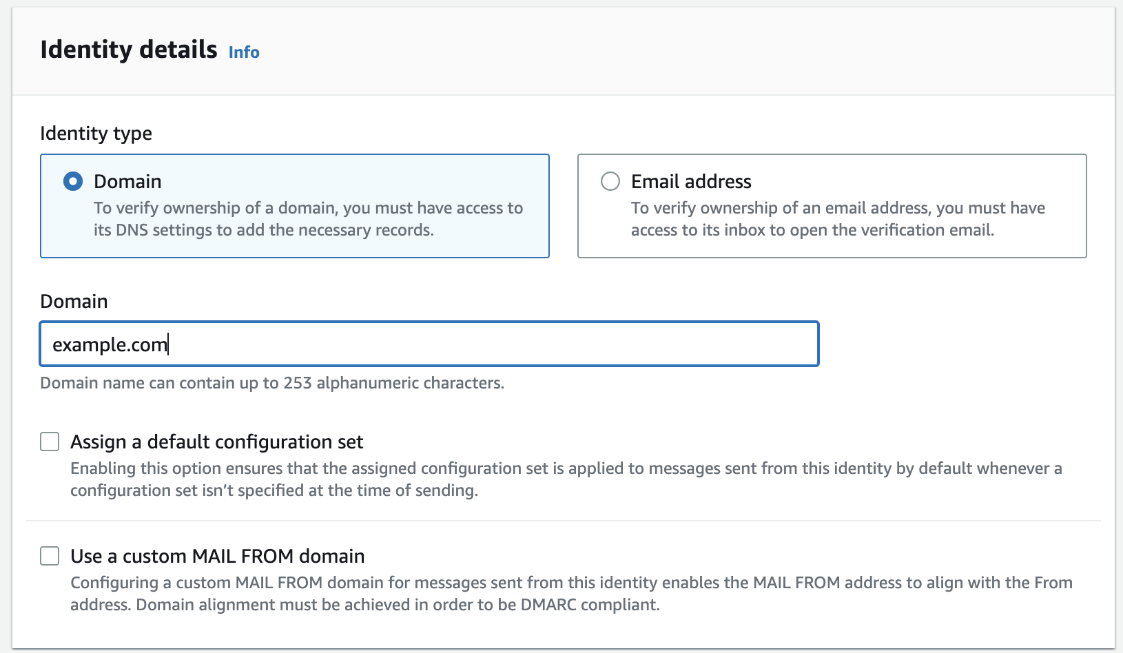
After your configuration set is created, you need to create Amazon SES event destination. Amazon SES will send all email deliverability events you intend to track to this event destination. In this blog the event destination is Amazon CloudWatch.

    1. Sign in to the Amazon SES console.
    2. In the navigation pane, under Configuration, choose Configuration sets. Choose Create set.
    3. Enter Configuration set name, leave the rest of fields to default, scroll to the send and click on Create set.
    4. Under configuration set home page click on Event destinations tab and select Add destination
    5. Add SES event destination to configuration set
    6. Under Select event types, check Sends, Deliveries, Hard bounces and Complaints boxes and click Next.
    7. selecting event types to track
    8. Under Specify destination, Select Amazon CloudWatch.
    9. Select event destination as Amazon CloudWatch
    10. Name – enter the name of the destination for this configuration set. The name can include letters, numbers, dashes, and hyphens. (example : Tracking_per_Domain)
    11. Under Amazon CloudWatch dimensions, Select Value source: Message tag , Dimension name: ses:from-domain and Default value: example.com (you will need to add the verified domain name you want to track) as shown below:
    12. add message auto-tag as CloudWatch dimension to track
    13. Review, When you are satisfied that your entries are correct, Click Add destination to add your event destination.

Send a test email via Amazon SES mailbox simulator to trigger events in CloudWatch custom metric.

After selected Amazon CloudWatch as event destination , Amazon CloudWatch will create a custom metric with the auto-tag dimension and value you chose. For this custom metric to appear in CloudWatch Console, you must send an email to trigger each selected event. We recommend using the Amazon SES Mailbox Simulator to avoid generating real bounces or complaints that could impact your account’s reputation.

In the below section, This blog will show how to send those test emails to the following recipients manually using CLI. If you would like to use the console method to send those emails. you will need to send three separate test emails since the console will only allow one recipient per message:

Amazon SES Mailbox Simulator recipients to trigger the events in CloudWatch metrics:
[email protected]
[email protected]
[email protected]

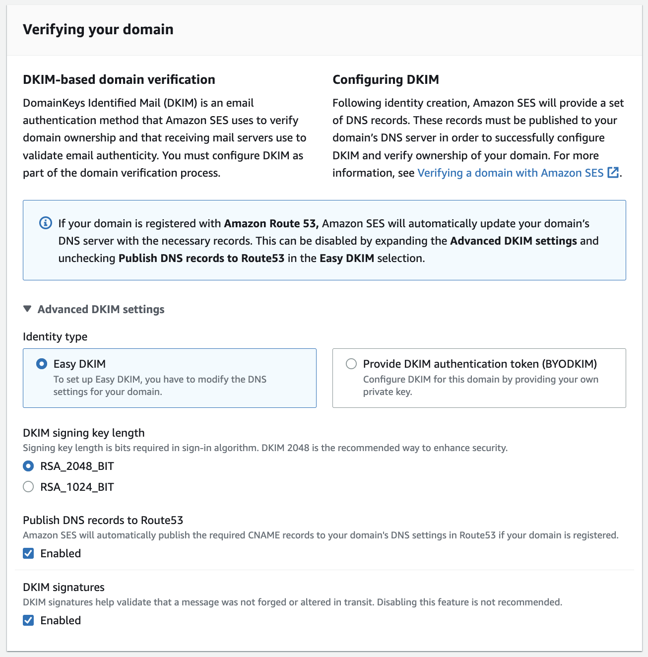
Note: You must pass the name of the configuration set when sending an email. This can be done by either specifying the configuration set name in the headers of emails, or specifying it as a default configuration set. This can be done at the time of identity creation, or later while editing a verified identity.

The following example uses send-emailCLI command to send a formatted email to the Amazon SES simulator recipients:

Before you run any commands, set your default credentials by following Configuring the AWS CLI. The IAM user must has “ses:SendEmail” permission to send email.

  1. Navigate to your terminal where the AWS CLI is installed and configured. Create message.json file for the message to send and add the following content:
  2. {
    "Subject": {
    "Data": "Testing CW events with email simulator",
    "Charset": "UTF-8"
    },
    "Body": {
    "Text": {
    "Data": "This is the message body of testing CW events with email similulator.",
    "Charset": "UTF-8"
    }
    }
    }
  3. Create a destination.json file to add Amazon SES simulator recipients for bounces, complaints and delivery events as shown below:
  4. { 
    
    "ToAddresses": ["[email protected]", "[email protected]" , "[email protected]"]
    
    }
  5. Send a test email using send-email CLI command to send a formatted email to the Amazon SES simulator recipients:
  6. aws ses send-email --from [email protected] --destination file://destination.json --message file://message.json --configuration-set-name SES_Config_Set --region <AWS Region>
  7. After the message sent, you are expected to see the following output:
  8. {
    
    "MessageId": "EXAMPLEf3a5efcd1-51adec81-d2a4-4e3f-9fe2-5d85c1b23783-000000"
    
    }

Now you sent a test email to trigger the events you want to track in CloudWatch custom metrics. Lets create the CloudWatch dashboard to see those metrics.

Create CloudWatch dashboard to track the email deliverability events for my domain.

  1. Sign in to the Amazon CloudWatch console.
  2. In the navigation pane, choose Dashboards, and then choose Create dashboard.
  3. In the Create new dashboard dialog box, enter a name like ‘CW_Domain_Tracking’ for the dashboard, and then choose Create dashboard.
  4. In the Add Widget dialog box, Choose Number to add a number displaying a metric to the dashboard and then choose Next
  5. Under Add metric graph, click on edit sign to rename the graph with your domain example.com . this will make it easy for you to select the dashboard of the domain if you have multiple domains.
  6. In the Browse tab , Select the AWS region where you are running your SES account and in the search bar, search for “ses:from-domain”.
  7. You will get four metrics returned with your domain name “example.com”. Select checkbox beside the four metrics and click Create widget.
  8. CloudWatch dashboard with the metrics
  9. Save dashboard in the top right corner of the dashboard page to save the widget settings.
  10. Save CloudWatch dashboard settings

After the CloudWatch dashboard created, for any email you send from example.com domain with configuration set name passed in the email header, The email deliverability events will be counted in your CloudWatch metrics and you will be able to see them in the CloudWatch dashboard.

As an additional step. You can also setup a CloudWatch alarms for this custom metrics and add a threshold for each metric. When the metric breach the threshold, the alarm goes on and send an SNS notification to you to take the necessary actions.

Cleaning Up:

This setup includes Amazon CloudWatch and Amazon SES service charges. To avoid incurring any extra charges, remember to delete any resources created manually if you no longer need them for monitoring.

Resources to delete from Amazon SES console.

  1. In the navigation pane, under Configuration, choose Configuration sets.
  2. Check the box beside Configuration set you created and select Delete.

Resources to delete from Amazon CloudWatch console.

  1. In the navigation pane, choose Dashboards, and then choose the dashboard you created.
  2. In the upper-right corner of the graph that you want to remove, choose Actions, and then choose Delete Dashboard.
  3. Save dashboard.

Conclusion:

You have now seen how to configure Amazon SES to track email deliverability at domain level with CloudWatch dashboard. Tracking email deliverability for emails you send from each domain is essential for business continuity, billing purposes or incidents investigations. Using SES message auto-tags and CloudWatch metrics you can identify the domains that have low email deliverability quickly and take necessary actions to maximize your email deliverability and take proactive actions before impacting the account’s ability to send emails from any other domains.

About the author:

Alaa Hammad

Alaa Hammad is a Senior Cloud Support Engineer at AWS and subject matter expert in Amazon Simple Email Service and AWS Backup service. She has a 10 years of diverse experience in supporting enterprise customers across different industries. She enjoys cooking and try new recipes from different cuisines.

Use AWS Private Certificate Authority to issue device attestation certificates for Matter

Post Syndicated from Ramesh Nagappan original https://aws.amazon.com/blogs/security/use-aws-private-certificate-authority-to-issue-device-attestation-certificates-for-matter/

In this blog post, we show you how to use AWS Private Certificate Authority (CA) to create Matter device attestation CAs to issue device attestation certificates (DAC). By using this solution, device makers can operate their own device attestation CAs, building on the solid security foundation provided by AWS Private CA. This post assumes that you are familiar with the public key infrastructure (PKI) — if needed, you can review the topic What is public key infrastructure?.

Overview

Matter, governed by the Connectivity Standard Alliance (CSA), is a new open standard for seamless and secure cross-vendor connectivity for smart home devices. It provides a common language for devices manufactured by different vendors to communicate on a smart home network by using the Wi-Fi and Thread wireless protocols. The Matter 1.0 specification, released in October 2022, supports smart home bridges and controllers, door locks, HVAC controls, lighting and electrical devices, media devices, safety and security sensors, and window coverings and shades. Future versions of the Matter specification will support additional smart home devices such as cameras, home appliances, robot vacuums, and other market segments such as electric vehicle (EV) charging and energy management.

To help achieve security and interoperability, Matter requires device certification and authenticity checks before devices can join a smart home network (known as the Matter fabric). The authenticity of a Matter device is established by using an X.509 certificate called a DAC, which is provisioned by device makers. When a customer purchases a Matter-compliant smart home device and uses a smart home hub to add that device to their Matter fabric, the hub validates the DAC before allowing the device to operate on the smart home’s Matter fabric.

Matter requires DACs to be issued by a device attestation CA that is compliant with the Matter PKI certificate policy (CP). Device vendors can use AWS Private CA to host their device attestation CAs. AWS Private CA is a highly available service that helps organizations secure their applications and devices by using private certificates. In Q1 2023, AWS Private CA launched support for Matter certificates, published the Matter PKI Compliance Customer Guide, and released open source samples to help customers create and operate Matter-compliant device attestation CAs.

In this post, we demonstrate how to build a Matter device attestation CA hierarchy by using AWS Private CA. The examples will use AWS Cloud Development Kit (AWS CDK) and AWS CloudFormation to create and provision the CAs and to issue Matter-compliant DACs. We also show how you can configure other AWS services like Amazon CloudWatch, AWS CloudTrail, and Amazon Simple Storage Service (Amazon S3) to help perform the event logging, record keeping, and audit log retention that is required in the Matter standard.

The Matter CA hierarchy for DACs

When a smart home device vendor makes the decision to adopt the Matter standard, they first apply to the CSA to get a vendor ID for their organization, and one or more product IDs for the products that will be Matter-certified. Using the vendor ID and product ID, the vendor can then set up their Matter CA hierarchy to issue DACs that will be provisioned on to their Matter-certified devices. Matter prescribes a two-level CA hierarchy for issuing DACs. The product attestation authority (PAA) is at the top of the hierarchy and forms the root of trust for the DACs that chain up to it. The product attestation intermediate (PAI) is at the second level of the CA hierarchy and is the CA that issues DACs. Figure 1 illustrates a sample Matter CA hierarchy for a vendor that manufactures devices with two different product IDs.

Figure 1: Matter CA three-tier hierarchy and the role of PAA, PAIs, and DACs

Figure 1: Matter CA three-tier hierarchy and the role of PAA, PAIs, and DACs

PAA certificates must be approved by the CSA before they are made available to the Matter community through the Distributed Compliance Ledger (DCL). The DCL is a shared database based on blockchain technology that holds the data elements that are necessary to attest the validity of a Matter device. CSA provides access to a public DCL node that it maintains, and private nodes can be created for dedicated access. To indicate whether a particular device is Matter compliant, a certification declaration (CD) is used. A CD is a CSA-created cryptographic document encoded in the Cryptographic Message Syntax (CMS) format described in RFC 5652. The data elements in the DCL include the list of PAAs (the roots of trust) and the vendor IDs, product IDs, and CD for each Matter certified product. The DCL also contains a description of each Matter certified product, which includes elements such as the device name, vendor, firmware version, and localized strings to support internationalization.

After the Matter CA hierarchy is set up, the CA operator must complete a certification practice statement (CPS) that describes how the CA operator will comply with the physical, operational, and logical controls specified in the Matter PKI CP. These controls address a large list of scenarios. These include the creation of the CA keys, storage of these key pairs, physical access controls for the HSMs, and separation of roles that perform administrative and operational tasks. The CA operators must submit their CPS, along with the PAA certificate, to the CSA for final approval. After the CPS is approved by the CSA, the PAA certificate is added to the list of approved Matter root certificates. This will now allow a Matter-compliant smart home network hub to verify the validity of the DAC that is provisioned on the Matter-certified device.

Build Matter CA hierarchies by using AWS Private CA

AWS Private CA has open sourced samples on GitHub that help you to create Matter-ready CA hierarchies and can issue DACs for your devices. These samples use the AWS CDK and CloudFormation templates to set up and configure services like Amazon CloudWatch, AWS CloudTrail and Amazon S3, to help you meet the Matter PKI compliance requirements. In the following sections, we walk you through an introduction to these samples, and discuss how you can use them to build your Matter CA hierarchies in AWS Private CA.

Solution architecture and building blocks

Figure 2 shows the Matter device attestation PKI architecture that is created when you run the GitHub samples. The architecture works as follows:

  1. A PAA is created by a PKI administrator, using the generatePaa key.
  2. You create PAIs by using the generatePaiCnt key in a single AWS Region, or you can choose to house the PAIs in different Regions.
  3. AWS CloudTrail captures the AWS API actions that are performed.
  4. Amazon CloudWatch receives a stream of filtered events specific to AWS Private CA and stores it in a dedicated MatterAudit log group.
  5. The logs are stored in Amazon S3 buckets.
  6. Logs can only be read by using the auditor-specific AWS Identity and Access Management (IAM) role that is configured for read-only access.
  7. The sample script configures the S3 buckets to automatically move log data to Amazon S3 Glacier storage by using S3 Lifecycle rules (Figure 2 shows an example of monthly backup plan for S3), in order to meet the long-term log retention requirements of the Matter standard.
  8. To issue DACs by using the PAIs created by the samples, you upload your certificate signing requests (CSRs) to the input/output S3 bucket.
  9. New CSRs are picked up by an AWS Lambda function through the use of Amazon Simple Queue Service (Amazon SQS).
  10. The DAC Signing Lambda function uses a PAI to generate a certificate.
  11. The Lambda function writes the generated certificates (which are the DACs) in the input/output S3 bucket in the Privacy Enhanced Mail (PEM) format.
Figure 2: Matter device attestation PKI architecture topology that uses AWS Private CA

Figure 2: Matter device attestation PKI architecture topology that uses AWS Private CA

Prerequisites

For a typical deployment, make sure you have a working host with the following software dependencies installed:

Using the following Git command, download sample scripts from the Matter PKI CDK samples on GitHub.

$ git clone https://github.com/aws-samples/aws-private-ca-matter-infrastructure.git
$ cd aws-private-ca-matter-infrastructure

Finally, set up the AWS CDK Toolkit with your AWS account’s credentials (see the AWS Cloud Development Kit documentation for details).

Deploy the PAA

The first step is to create and deploy a Matter PAA by running the following command:

$ cdk deploy ‐‐context generatePaa=1 ‐‐parameters vendorId=FFF1 ‐‐parameters validityInDays=3600

After the command completes, you should see the following output:

MatterStackPAA.CloudTrailArn = arn:aws:cloudtrail:us-east-1:111111111111:trail/MatterStackPAA-MatterAuditTrail586D7D12-akSFjLJyEumz

MatterStackPAA.LogGroupName = MatterAudit

MatterStackPAA.PAA = VID=FFF1 CN=PAA arn:aws:acm-pca:us-east-1:111111111111:certificate-authority/99999999-9999-9999-9999-999999999999

MatterStackPAA.PAACertArn = arn:aws:acm-pca:us-east-1:111111111111:certificate-authority/99999999-9999-9999-9999-999999999999/certificate/99999999999999999999999999999999

MatterStackPAA.PAACertLink = https://console.aws.amazon.com/acm-pca/home?region=us-east-1#/details?arn=arn:aws:acm-pca:us-east-1:111111111111:certificate-authority/99999999-9999-9999-9999-999999999999&tab=certificate

Stack ARN:
    arn:aws:cloudformation:us-east-1:111111111111:stack/MatterStackPAA/11111111-1111-1111-1111-111111111111

Note the following fields in the output:

  • CloudTrailArn — The Amazon Resource Name (ARN) of the CloudTrail trail that is collecting logs of performed operations.
  • LogGroupName — The ARN of the CloudWatch log group where you can find logs of Matter-relevant operations.
  • PAA — The vendor ID, common name, and ARN of the AWS Private CA root certificate authority created as the PAA.
  • PAACertArn — The ARN of the certificate of the PAA in AWS Private CA.
  • PAACertLink — The link to the PAA certificate in the AWS Private CA console.

Deploy one or more PAIs

To deploy two PAIs that chain up to the PAA that you created in the previous step, run the following command:

$ PAA_ARN=$(awk '/MatterStackPAA.PAA = /{ print substr($0, match($0, "arn")); }' DeployPAA.log)
$ cdk deploy --context generatePaiCnt=2 ‐‐parameters vendorId=FFF1 ‐‐parameters productIds=0100,0102 ‐‐parameters validityInDays=365 ‐‐parameters paaArn=$PAA_ARN

If you want to create more or fewer PAIs, you can modify the generatePaiCnt and productIds parameters to reflect the correct number of PAIs that you want.

After the command completes, you should see the following output:

MatterStackPAI.CertArnPAI0 = arn:aws:acm-pca:us-east-1:111111111111:certificate-authority/99999999-9999-9999-9999-999999999999/certificate/11111111111111111111111111111111

MatterStackPAI.CertArnPAI1 = arn:aws:acm-pca:us-east-1:111111111111:certificate-authority/99999999-9999-9999-9999-999999999999/certificate/22222222222222222222222222222222

MatterStackPAI.CertLinkPAI0 = https://console.aws.amazon.com/acm-pca/home?region=us-west-1#/details?arn=arn:aws:acm-pca:us-west-1:111111111111:certificate-authority/11111111-1111-1111-1111-111111111111&tab=certificate

MatterStackPAI.CertLinkPAI1 = https://console.aws.amazon.com/acm-pca/home?region=us-west-1#/details?arn=arn:aws:acm-pca:us-west-1:111111111111:certificate-authority/22222222-2222-2222-2222-222222222222&tab=certificate

MatterStackPAI.PAI0 = VID=FFF1 PID=0100 CN=PAI0 arn:aws:acm-pca:us-west-1:111111111111:certificate-authority/11111111-1111-1111-1111-111111111111

MatterStackPAI.PAI1 = VID=FFF1 PID=0102 CN=PAI1 arn:aws:acm-pca:us-west-1:111111111111:certificate-authority/22222222-2222-2222-2222-222222222222

Note the following fields in the output:

  • CertArnPAI0 — The ARN of the certificate of the first PAI in AWS Private CA.
  • CertArnPAI1 — The ARN of the certificate of the second PAI in AWS Private CA.
  • CertLinkPAI0 — The link to the first PAI certificate in the AWS Private CA console.
  • CertLinkPAI1 — The link to the second PAI certificate in the AWS Private CA console.
  • PAI0 — The vendor ID, product ID, common name, and ARN of the AWS Private CA subordinate certificate authority created as the first PAI.
  • PAI1 — The vendor ID, product ID, common name, and ARN of the AWS Private CA subordinate certificate authority created as the second PAI.

Deploy multi-Region PAIs

The following command is an example of how you can generate a PAI in a different Region. To specify a Region, either use the CDK_DEFAULT_REGION environment variable or specify a different AWS profile by using the –profile parameter (see AWS CDK documentation for more details).

$ CDK_DEFAULT_REGION=us-east-1
$ cdk deploy ‐‐context generatePaiCnt=1 ‐‐parameters vendorId=FFF1 ‐‐parameters productIds=0100 ‐‐parameters validityInDays=365 ‐‐parameters paaArn=<PAA-ARN-FROM-PAA-OUTPUT>

Issue DACs

After the Matter CA hierarchy is set up, you can issue DACs by writing your CSRs directly to the DacInputS3ToSQSS3Bucket S3 bucket. The SqsToDacIssuingLambda function signs the CSRs by using the specified PAI to create a DAC, and then the function writes that DAC back to the S3 bucket.

To test this procedure by using OpenSSL

  1. Use the following command to create a key pair for the DAC:
    $ openssl ecparam -name prime256v1 -out certificates/ecparam

  2. Create the DAC CSR with DAC as the common name; the following is an example:
    $ openssl req -config certificates/config.ssl -newkey param:certificates/ecparam -keyout key-DAC.pem -out cert-DAC.csr -sha256 -subj "/CN=DAC"

  3. Request CSR signing by using a PAI identified by its UUID:
    $ aws s3 cp cert-DAC.csr s3://Matterstackpai-dacinputs3tosqss3bucket<remainder of your bucket name>/arn:aws:acm-pca:<region>:<account>:certificate-authority/<PAI UUID>/<PID>/cert-DAC.csr

  4. The PAI will respond with the certificate as soon as it finishes processing the CSR, and the certificate will be made available in the same S3 bucket:
    $ aws s3 cp s3://Matterstackpai-dacinputs3tosqss3bucket<remainder of your bucket name>/arn:aws:acm-pca:<region>:<account>:certificate-authority/<PAI UUID>/<PID>/cert-DAC.pem

Audit trails, record keeping, and retention

The Matter PKI CP mandates controls and processes that are required to operate Matter device attestation CAs. The Matter PKI CDK samples on GitHub configure IAM roles, AWS CloudTrail, Amazon CloudWatch, and Amazon S3 to help you meet these requirements. Specifically, the samples configure the following:

  • Permissions
    • The /MatterPKI/MatterIssueDACRole role, for issuing and revoking DACs from PAIs in AWS Private CA.
    • The /MatterPKI/MatterIssuePAIRole role, for issuing and revoking PAIs from the PAA in AWS Private CA.
    • The /MatterPKI/MatterManagePAARole role, for monitoring and managing the PAA.
    • The /MatterPKI/MatterAuditorRole role, for viewing, collecting, and managing the logs that pertain to Matter PKI resources.
  • Logging
    • Audit logs should be maintained for operations performed in AWS that are related to the Matter PKI. This is accomplished by using AWS CloudTrail to store logs of API calls in S3.
    • In order to preserve the integrity of the data in the audit logging S3 bucket, the sample scripts configure S3 Object Lock to make objects write-once, read-many.
    • A resource policy is applied to the S3 bucket that grants IAM role access only to the auditor.
    • Data in this S3 bucket is backed up to a vault by using AWS Backup. From there, the data can be restored in case of an emergency.
    • The logs are retained in S3 for two months after creation and then are automatically moved into S3 Glacier for the rest of their five-year lifecycle, where they can be restored if necessary.
    • In order to make sure that the logs can be quickly queried by an auditor, the sample script sets up CloudTrail to continuously send events that are filtered to include only events relevant to Matter PKI to the AWS CloudWatch log group MatterAudit. You should restrict access to the stored logs by enabling log integrity validation to assure that the log remains computationally infeasible to modify, delete or forge.

Verify and validate certificates for Matter compliance

The Matter standards working group provides the CHIP Certificate Tool (chip-cert), a CLI utility that you can use to verify the conformance of the certificates that form a DAC chain. If you use the sample script we provided earlier to generate DACs, this tool is run as part of the certificate issuance process to verify that the certificate and chain are Matter compliant and no misconfiguration has taken place.

Use the following command to validate a DAC chain by using chip-cert manually.

$./chip-cert validate-att-cert ‐‐dac <dac-certificate-file-in-PEM> ‐‐pai <pai-certificate-file-in-PEM> ‐‐paa <paa-certificate-file-in-PEM> 

Best practices for assuring security, scalability, and resiliency

For a list of best practices and recommendations for using AWS Private CA effectively, see AWS Private CA best practices.

Cost considerations

When you install the Matter PKI CDK, you will incur charges for the deployment and use of AWS Private CA and the associated services. To delete a private CA permanently, see Deleting your private CA.

Conclusion

In this blog post, we discussed in depth the use of AWS Private CA to create and operate Matter device attestation CAs in order to issue DACs. We walked you through how you can use our open source samples on GitHub to create Matter PAAs and PAIs, and how to configure other AWS services like Amazon CloudWatch, AWS CloudTrail and Amazon S3 to help you meet the compliance requirements that are stipulated by the Matter PKI CP. We also showed you how you can use the Matter PAIs to issue DACs for your smart home devices and verify that the issued DACs meet the Matter requirements. To learn more about using the GitHub samples, see the README file located in the GitHub repository. We welcome your feedback to help us improve the samples.

 
If you have feedback about this post, submit comments in the Comments section below. If you have questions about this post, contact AWS Support.

Want more AWS Security news? Follow us on Twitter.

Ramesh Nagappan

Ramesh Nagappan

Ramesh is a Principal Security Engineer in the Devices and Services Trust Security (DSTS) organization at Amazon. With extensive experience, he remains focused on technologies related to applied cryptography, identity management, IoT, and Cloud infrastructure.

Leonid Wilde

Leonid Wilde

Leonid is a Software Engineer in the AWS Cryptography organization who also worked in various teams within Amazon. In his previous life, he worked on various products involving cryptographic algorithms, compilers, drivers, networking, and more.

Lukas Rash

Lukas Rash

Lukas is a Software Engineer in the AWS Cryptography organization. He is passionate about building robust cloud services to help customers improve the security of their systems.

Lorey Spade

Lorey Spade

Lorey is a Senior Industry Specialist in the AWS Cryptography organization, specializing in public key infrastructure compliance. She has extensive experience in the area of information technology auditing and compliance.

How to send your first email on SES

Post Syndicated from Dustin Taylor original https://aws.amazon.com/blogs/messaging-and-targeting/how-to-send-your-first-email-on-ses/

Introduction

Sending your first email on any service can be complicated. In this blog we will walk you through how to send your first email on Amazon Simple Email Service (SES) through the SES Console and to direct you to examples of how you can send email through the AWS SDK. Our public documentation includes additional information on how you can configure SES. We encourage you to read through these documents to learn about these other mechanisms in the future.

Getting Started

Getting started with sending an email on SES requires three actions which are: 1) verifying a domain or email address 2) requesting production access to SES and 3) sending your first email. Let’s walk through each of these steps and send our first email.

Verifying an Identity

To start, you will configure what email address or domain your customers will receive emails from. As part of this verification, you will need to be able to either receive a confirmation email at the email address you are trying to setup, or to publish CNAME records for your intended domain. Generally, we recommend using a domain for your email sending as this gives you the ability to set up SPF, DKIM, and DMARC alignment which will increase recipient trust in your emails. Email addresses can be used for account-specific email sending where a customer may not own a domain, but this type of use-case is prone to receiving entities having low trust in the sender and a lower probability of inbox placement. For more in-depth instructions please review our public documentation as I will briefly touch on the most important pieces to verifying a domain or email address.

To verify an identity, you can go to the SES Console and click the ‘Verified identities’ link on the left-hand side of the screen. It will then present you with a list of verified domains or email addresses currently in your account if they were previously verified. There is a yellow button that states ‘Create identity’, when you click this you will be presented with a screen to choose whether to verify an email address or domain.

Email Address Verification

To verify an email address, you will be prompted with the following dialog:

The dialog presented to a sender when they choose to verify an email address in the SES console.

To verify an email address to use as your sending identity, you will include the address in the ‘Email address’ field and then click the ‘Create identity’ button. This will trigger an automated email to the address with a verification link that will need to be clicked to verify ownership of the email address. Once verified, you can begin sending emails from your new email address identity.

Domain Verification

To start verifying a domain you will click the ‘Verified identities’ option from the ‘Configuration’ dropdown which can be found on the left side of the screen. When choosing to verify a domain, you will be presented with a series of dialogs which include:

The dialog presented to a sender that prompts a decision to verify a domain or email address.

Here you will need to include the domain you intend to use for email sending. If you are keeping to a basic configuration on SES this will be the only data you need to add to this dialog. However, it is recommended to also use a custom mail-from. A custom mail-from is a way for you to remove the amazonses.com domain from your mail-from header to ensure domain alignment throughout your headers. You can find more information about the custom mail-from addresses in our documentation.

After finishing your changes in the first dialog you will then be presented with a second dialog that looks like the following:

The dialog which allows a sender to verify the domain they intend to use to send email.

To verify the domain, you will need to utilize either the Easy DKIM feature, or to provide a DKIM authentication token if you plan to DKIM sign your own messages. In selecting the ‘Easy DKIM’ option, you will be presented with the option to use either 1024 bit or 2048 bit signing key length. We would recommend utilizing the 2048 bit signing key length for most customers as this is the more secure key.

If you use Amazon Route53 as your DNS provider, SES can automatically publish DNS records for your domain. If not, this step will require you to edit your DNS records to include three CNAME records which are used for the DKIM signature process and as a mechanism to prove domain ownership. An example of the CNAME records is as follows:

An example dialog of the CNAME records that are generated when attempting to verify an identity.

Once you have placed these DNS records SES will periodically attempt to look-up the records to change the status of your domain verification. If SES doesn’t automatically update the status, you are presented with the option to force another check to verify the records are present.

After your domain verification is successful, you are now ready to send emails from any email address for your domain.

Requesting Production Access

Now that you’ve verified an identity, the next step is to be able to send an email to an unverified identity you will need to request production access. If you only want to test to your own domain or email address you can skip this step until you are ready to send to unverified recipients.

Note: This is region-based, a request for production access is limited to the region in which you are requesting. 

To begin this process, you will navigate to the SES Console and the ‘Account dashboard’ section. Once you are on this page you will be presented with the following dialog at the top of your screen.

Clicking the ‘Request production access’ button will then navigate to the ‘Request details’ page which you can reference below.

The dialog from the SES console showing that the SES account is still in the sandbox.
Fill out each section with the details of your mail-type, website URL, use case description, and then acknowledging that you have read and agree to the AWS Service Terms and Acceptable Use Policy (AUP). When filling out the use case description, provide as much detail as you can for your request as our teams will review to determine if we need more information before approving or denying your request. An example of a good use case description would look like the following:

“Example.com is the domain my company intends to use to send our transactional emails. Our recipients are all customers who have either signed up for an account, requested a new password, or have made purchases through our website. We require confirmation of opt-in for all our new accounts and if no confirmation is received, we do not attempt to send an email to that address.”

Note: SES will review your production access request and will provide feedback on your use case and whether it could pose a risk to the sending reputation of SES, our customers, or your own sending domain.

Finally, click the ‘Submit request’ button to submit your request for production access. This will create an AWS Support case and will be reviewed by our team. These requests are reviewed with a 24-hour Service Level Agreement (SLA). While you are waiting for production access you can send test emails to any of the Mailbox Simulator endpoints or to your own verified domain(s) or email address(es).

Sending Your First Email

From the Console

To send your first email from the SES Console you will need to start by clicking the ‘Verified identities’ option from the ‘Configuration’ dropdown which can be found on the left side of the screen. From here you will select the domain and/or email address you want to send your email from and then click the ‘Send test email’ button, which will open the following screen:

The message details dialog where a sender can send an email from the SES console

From here you will fill out the ‘From-address’ box with the local name (anything before the @ sign) that you want to use to send the email. If you want to test SES functionality you can choose any of the dropdown events present, or you can choose the ‘Custom’ option which will allow you to set a ‘Custom recipient’ address of your choosing. Then you will fill out the ‘Subject’ and ‘Body’ fields with the content you will use for this first test email and then click the ‘Send test email’ button.

Congratulations, you’ve sent your first email from the SES Console! Now, utilizing SES to send single emails from the console isn’t the most scalable way to send email. In the next section, I will provide you links to our documentation for the 5 programming languages supported with the AWS SDK so that you can begin building your integration with SES.

From Code

The AWS Documentation includes some code snippets on how to send an email with SES via the AWS SDK. You can find examples of how to send an email from languages such as: .NET, Java, PHP, Ruby, and Python. We highly recommend reviewing our documentation to see these introductory code snippets to get you started.

Conclusion

Hopefully this blog post has aided you in your journey to send your first email through SES. From verifying a domain, requesting production access, and finally sending an email through the console. Take this knowledge and build upon it for future success in sending email through SES. Happy sending!

Intel Manufacturing Gets its Own Profit and Loss Potentially Gearing Up for a Spin-Off

Post Syndicated from Patrick Kennedy original https://www.servethehome.com/intel-manufacturing-gets-its-own-profit-and-loss-potentially-gearing-up-for-a-spin-off/

Intel is giving its manufacturing arm its own P&L to help drive cost reductions. The announcement feels a lot like it is gearing for a split

The post Intel Manufacturing Gets its Own Profit and Loss Potentially Gearing Up for a Spin-Off appeared first on ServeTheHome.

Accelerate onboarding and seamless integration with ThoughtSpot using Amazon Redshift partner integration

Post Syndicated from Antony Prasad Thevaraj original https://aws.amazon.com/blogs/big-data/accelerate-onboarding-and-seamless-integration-with-thoughtspot-using-amazon-redshift-partner-integration/

Amazon Redshift is a fast, petabyte-scale cloud data warehouse that makes it simple and cost-effective to analyze all of your data using standard SQL. Tens of thousands of customers today rely on Amazon Redshift to analyze exabytes of data and run complex analytical queries, making it the most widely used cloud data warehouse. You can run and scale analytics in seconds on all your data without having to manage your data warehouse infrastructure.

Today, we are excited to announce ThoughtSpot as a new BI partner available through Amazon Redshift partner integration. You can onboard with ThoughtSpot in minutes directly from the Amazon Redshift console and gain faster data-driven insights. Businesses typically look at ways to derive business insights. This is where modern analytics providers such as ThoughtSpot provide value. With its powerful AI-based search, live visualizations, and developer tools and APIs for sharing embedded analytics, ThoughtSpot democratizes access to data by providing self-service tools for all users.

In this post, you will learn how to integrate seamlessly with ThoughtSpot from the Amazon Redshift console. With the loosely coupled nature of the modern data stack, it’s simple to connect Amazon Redshift with ThoughtSpot. No data movement or replication is required.

ThoughtSpot: Live analytics for your modern data stack

Static dashboards cannot deliver consistent and reliable insights at the speed and global scale that customers demand. They lack the following:

  • Opportunities for collaboration
  • Discovery and reusability
  • Secure remote data and insight access
  • Rapid use case development with single-touch insight provisioning

ThoughtSpot empowers everyone to create, consume, and operationalize data-driven insights. ThoughtSpot consumer-grade search and AI technology delivers true self-service analytics that anyone can use, while its developer-friendly platform ThoughtSpot Everywhere makes it easy to build interactive data apps that integrate with your existing cloud provider.

As organizations increasingly move to the cloud, ThoughtSpot helps them quickly unlock value from their investment. ThoughtSpot’s simple search functionality enables you to easily ask and answer data questions in seconds to unearth impactful insights directly in Amazon Redshift. ThoughtSpot for AWS provides enterprises with more freedom and flexibility by eliminating the need to move data between cloud sources so that businesses can immediately benefit from data-driven decision-making.

ThoughtSpot is an AWS Data and Analytics Competency Partner with the Amazon Redshift Ready product designation. ThoughtSpot is also part of the Powered by Amazon Redshift program.

Integrate ThoughtSpot using Amazon Redshift partner integration

Complete the following steps to integrate ThoughtSpot with Amazon Redshift:

  1. On the Amazon Redshift console, choose Clusters in the navigation pane.
  2. Select your cluster and on the Actions menu, choose Add AWS Partner integration.

Alternatively, you can choose your individual cluster and on its details page, choose Add partner integration.

  1. Select ThoughtSpot as your desired BI partner.
  2. Choose Next.

  1. Choose Add partner.

  1. Log in on the ThoughtSpot landing page.

  1. Select Continue to Setup.

  1. On the Amazon Redshift connection details page, enter your Amazon Redshift database password for Password.
  2. Choose Continue.

To connect to your Amazon Redshift cluster, make sure to enable the Publicly accessible option and allow list the ThoughtSpot IP in your Amazon Redshift cluster’s security group.

  1. Select your desired tables and choose Update.
  2. If a prompt appears, choose Update again.

After you have successfully integrated with ThoughtSpot, you will see an Active status in the Integrations section on the Amazon Redshift console.

Congratulations! You’re now ready to start visualizing data using ThoughtSpot. The following example shows you trends in sales growth YTD, current sales trends across regions, and a comparison between product type sales between the current year and the previous year. You can slice and dice the dataset based on the granularity defined by the user.

Partner feedback

“ThoughtSpot is thrilled to expand our long-time cooperation with AWS with the announcement of our Amazon Redshift partner integration. Leading organizations are already extracting value from their data using AI-powered analytics on Amazon Redshift, and today we are making it even more frictionless for Amazon Redshift users to launch ThoughtSpot’s free trial to solve real problems quickly.”

– Kuntal Vahalia, SVP of WW Partners & APAC

Conclusion

In this post, we discussed how Amazon Redshift partner integration provides a fast-onboarding experience and allows you to create valuable business insights by integrating with ThoughtSpot. ThoughtSpot enables you to unlock the value of your modern data stack by empowering your entire organization with live analytics and data search, while Amazon Redshift provides a modern data warehouse experience for you to manage analytics at scale.

If you’re an AWS Partner and would like to integrate your product into the Amazon Redshift console, contact [email protected] for additional information and guidance. This console partner integration functionality is available to new and existing customers at no additional cost. To get started and learn more, see Integrating Amazon Redshift with an AWS Partner.


About the Authors

Antony Prasad Thevaraj is a Sr. Partner Solutions Architect in Data and Analytics at AWS. He has over 12 years of experience as a Big Data Engineer, and has worked on building complex ETL and ELT pipelines for various business units.

Maneesh Sharma is a Senior Database Engineer at AWS with more than a decade of experience designing and implementing large-scale data warehouse and analytics solutions. He collaborates with various Amazon Redshift Partners and customers to drive better integration.

[$] Merging copy offload

Post Syndicated from original https://lwn.net/Articles/935260/

Kernel support for copy offload is a feature that has been floating around
in limbo for a decade or more at this point; it has been implemented along
the way, but never merged. The idea is that the host
system can simply ask a block storage device to copy some data within the device
and it
will do so without further involving the host; instead of reading data into
the host so that it can be written back out again, the device circumvents
that process. At the
2023 Linux Storage, Filesystem,
Memory-Management and BPF Summit
, Nitesh Shetty led a storage and
filesystem session to discuss the current status of a patch set that he and
others have been working on, with an
eye toward getting something merged fairly soon.

Ethical Problems in Computer Security

Post Syndicated from Bruce Schneier original https://www.schneier.com/blog/archives/2023/06/ethical-problems-in-computer-security.html

Tadayoshi Kohno, Yasemin Acar, and Wulf Loh wrote excellent paper on ethical thinking within the computer security community: “Ethical Frameworks and Computer Security Trolley Problems: Foundations for Conversation“:

Abstract: The computer security research community regularly tackles ethical questions. The field of ethics / moral philosophy has for centuries considered what it means to be “morally good” or at least “morally allowed / acceptable.” Among philosophy’s contributions are (1) frameworks for evaluating the morality of actions—including the well-established consequentialist and deontological frameworks—and (2) scenarios (like trolley problems) featuring moral dilemmas that can facilitate discussion about and intellectual inquiry into different perspectives on moral reasoning and decision-making. In a classic trolley problem, consequentialist and deontological analyses may render different opinions. In this research, we explicitly make and explore connections between moral questions in computer security research and ethics / moral philosophy through the creation and analysis of trolley problem-like computer security-themed moral dilemmas and, in doing so, we seek to contribute to conversations among security researchers about the morality of security research-related decisions. We explicitly do not seek to define what is morally right or wrong, nor do we argue for one framework over another. Indeed, the consequentialist and deontological frameworks that we center, in addition to coming to different conclusions for our scenarios, have significant limitations. Instead, by offering our scenarios and by comparing two different approaches to ethics, we strive to contribute to how the computer security research field considers and converses about ethical questions, especially when there are different perspectives on what is morally right or acceptable. Our vision is for this work to be broadly useful to the computer security community, including to researchers as they embark on (or choose not to embark on), conduct, and write about their research, to program committees as they evaluate submissions, and to educators as they teach about computer security and ethics.

The paper will be presented at USENIX Security.

Crafting a better, faster code view

Post Syndicated from Joshua Brown original https://github.blog/2023-06-21-crafting-a-better-faster-code-view/

Reading code is not as simple as reading the text of a file end-to-end. It is a non-linear, sometimes chaotic process of jumping between files to follow a trail, building a mental picture of how code relates to its surrounding context. GitHub’s mission is to be the home for all developers, and reading code is one of the core experiences we offer. Every day, millions of users use GitHub to view and interact with code. So, about a year ago we set out to create a new code view that supports the entire code reading experience with features like a file tree, symbol navigation, code search integration, sticky lines, and code section folding. The new code view is powerful, intelligent, and interactive, but it is not an attempt to turn the repository browsing experience into an IDE.

While building the new code view, our team had a few guiding principles on which we refused to compromise:

  • It must add these powerful new features to transform how users read code on GitHub.
  • It must be intuitive and easy to use for all of GitHub’s millions of users.
  • It must be fast.

Initial efforts

The first step was to build out the features we wanted in a natural, straightforward way, taking the advice that “premature optimization is the root of all evil.”1 After all, if simple code satisfactorily solves our problems, then we should stop there. We knew we wanted to build a highly interactive and stateful code viewing experience, so we decided to use React to enable us to iterate more quickly on the user interface. Our initial implementation for the code blob was dead-simple: our syntax highlighting service converted the raw file contents to a list of HTML strings corresponding to the lines of the file, and each of these lines was added to the document.

There was one key problem: our performance scaled badly with the number of lines in the file. In particular, our LCP and TTI times measurably increased at around 500 lines, and this increase became noticeable at around 2,000 lines. Around those same thresholds, interactions like highlighting a line or collapsing a code section became similarly sluggish. We take these performance metrics seriously for a number of reasons. Most importantly, they are user-centric—that is, they are meant to measure aspects of the quality of a user’s experience on the page. On top of that, they are also part of how search engines like Google determine where to rank pages in their search results; fast pages get shown first, and the code view is one of the many ways GitHub’s users can show their work to the world.

As we dug in, we discovered that there were a few things at play:

  • When there are many DOM nodes on the page, style calculations and paints take longer.
  • When there are many DOM nodes on the page, DOM queries take longer, and the results can have a significant memory footprint.
  • When there are many React nodes on the page, renders and DOM reconciliation both take longer.

It’s worth noting that none of these are problems with React specifically; any page with a very large DOM would experience the first two problems, and any solution where a large DOM is created and managed by JavaScript would experience the third.

We mitigated these problems considerably by ensuring that we were not running these expensive operations more than necessary. Typical React optimization techniques like memoization and debouncing user input, as well as some less common solutions like pulling in an observer pattern went a long way toward ensuring that React state updates, and therefore DOM updates, only occurred as needed.

Mitigating the problem, however, is not solving the problem. Even with all of these optimizations in place, the initial render of the page remained a fundamentally expensive operation for large files. In the repository that builds GitHub.com, for example, we have a CODEOWNERS file that is about 18,000 lines long, and pushes the 2MB size limit for displaying files in the UI. With no optimizations besides the ones described above, React’s first pass at building the DOM for this page takes nearly 27 seconds.2 Considering more than half of users will abandon a page if it loads for more than three seconds, there was obviously lots of work left to do.

A promising but incomplete solution

Enter virtualization. Virtualization is a performance optimization technique that examines the scroll state of the page to determine what content to include in the DOM. For example, if we are viewing a 10,000 line file but only about 75 lines fit on the screen at a time, we can save lots of time by only rendering the lines that fit in the viewport. As the user scrolls, we add any lines that need to appear, and remove any lines that can disappear, as illustrated by this demo.3

This satisfies the most basic requirements of the page with flying colors. It loads on average more quickly than the existing experience, and the experience of scrolling through the file is nearly indistinguishable from the non-virtualized case. Remember that 27 second initial render? Virtualizing the file content gets that time down to under a second, and that number does not increase substantially even if we artificially remove our file size limit and pull in hundreds of megabytes of text.

Unfortunately, virtualization is not a cure-all. While our initial implementation added features to the page at the expense of performance, naïvely virtualizing the code lines delivers a fast experience at the expense of vital functionality. The biggest problem was that without the entire text of the file on the page at once, the browser’s built-in find-in-file only surfaced results that are visible in the viewport. Breaking users’ ability to find text on the page breaks our hard requirement that the page remain intuitive and easy to use. Before we could ship any of this to real users, we had to ensure that this use case would be covered.

The immediate solution was to implement our own version of find-in-file by implementing a custom handler for the Ctrl+F shortcut (⌘+F on Mac). We added a new piece of UI in the sidebar to show results as part of our integration with symbol navigation and code search.

Screenshot of the "find" sidebar, showing a search bar with the term "isUn" and a list offive lines of code from the current file that contain that string, the second of which is highlighted as selected.

There is precedent for overriding this native browser feature to allow users to find text in virtualized code lines. Monaco, the text editor behind VS Code, does exactly this to solve the same problem, as do many other online code editors, including Repl.it and CodePen. Some other editors like the official Ruby playground ignore the problem altogether and accept that Ctrl+F will be partially broken within their virtualized editor.

At the time, we felt confident leaning on this precedent. These examples are applications that run in a browser window, and as users, we expect applications to implement their own controls. Writing our own way to find text on the page was a step toward making GitHub’s Code View less of a web page and more of a web application.

When we released the new code view experience as a private beta at GitHub Universe, we received clear feedback that our users think of GitHub as a page, not as an app. We tried to rework the experience to be as similar as possible to the native implementation, both in terms of user experience and performance. But ultimately, there are plenty of good reasons not to override this kind of native browser behavior.

  • Users of assistive technologies often use Ctrl+F to locate elements on a page, so restricting the scope to the contents of the file broke these workflows.
  • Users rely heavily on specific muscle memory for common actions, and we followed a deep rabbit hole to get the custom control to support all of the shortcuts used by various browsers.
  • Finally, the native browser implementation is simply faster.

Despite plenty of precedent for an overridden find experience, this user feedback drove us to dig deeper into how we could lean on the browser for something it already does well.

Virtualization has an important role to play in our final product, but it is only one piece of the puzzle.

How the pieces fit together

Our complete solution for the code view features two pieces:

  1. A textarea that contains the entire text of the raw file. The contents are accessible, keyboard-navigable, copyable, and findable, yet invisible.
  2. A virtualized, syntax-highlighted overlay. The contents are visible, yet hidden from both mouse events and the browser’s find.

Together, these pieces deliver a code view that supports the complete code reading experience with many new features. Despite the added complexity, this new experience is faster to render than the static HTML page that has displayed code on GitHub for more than a decade.

A textarea and a read-only cursor

The first half of this solution came to us from an unexpected angle.

Beyond adding functionality to the code view, we wanted to improve the code reading experience for users of assistive technologies like screen readers. The previous code view was minimally accessible; a code document was displayed as a table, which created a very surprising experience for screen reader users. A code document is not a table, but likewise it is not a paragraph of text. To support a familiar interface for interacting with the code on the page, we added an invisible textarea underneath the virtualized, syntax-highlighted code lines so that users can move through the code with the keyboard in a familiar way. And for the browser, rendering a textarea is much simpler than using JavaScript to insert syntax-highlighted HTML. Browsers can render megabytes of text in a textarea with ease.

Since this textarea contains the entire text of the raw file, it is not just an accessibility feature, but an opportunity to remove our custom implementation of Ctrl+F in favor of native browser implementations.

Hiding text from Ctrl+F

With the addition of the textarea, we now have two copies of every line that is visible in the viewport: one in the textarea, and another in the virtualized, syntax-highlighted overlay. In this state, searching for text yields duplicated results, which is more confusing than a slow or unfamiliar experience.

The question, then, is how to expose only one copy of the text to the browser’s native Ctrl+F. That brings us to the next key part of our solution: how we hid the syntax-highlighted overlay from find.

For a code snippet like this line of Python:

print("Hello!")

the old code view created a bit of HTML that looks like this:

<span class="pl-en">print</span>(<span class="pl-s">"Hello!"</span>)

But the text nodes containing print, (,"Hello!", and ) are all findable. It took two iterations to arrive at a format that looks identical but is consistently hidden fromCtrl+F on all major browsers. And as it turns out, this is not a question that is very easy to research!

The first approach we tried relied on the fact that :before pseudoelements are not part of the DOM, and therefore do not appear in find results. With a bit of a change to our HTML format that moves all text into a data- attribute, we can use CSS to inject the code text into the page without any findable text nodes.

HTML

<span class="pl-en" data-code-text="print"></span>
<span data-code-text="("></span>
<span class="pl-s" data-code-text=""Hello!""></span>
<span data-code-text=")"></span>

CSS

[data-code-text]:before {
   content: attr(data-code-text);
}

But that’s not the end of the story, because the major browsers do not agree on whether text in :before pseudoelements should be findable; Firefox in particular has a powerful Ctrl+F implementation that is not fooled by our first trick.

Our second attempt relied on a fact on which all browsers seem to agree: that text in adjacent pseudoelements is not treated as a contiguous block of text.4 So, even though Firefox would find print in the first example, it would not find print(. The solution, then, is to break up the text character-by-character:

<span class="pl-en">
   <span data-code-text="p"></span>
   <span data-code-text="r"></span>
   <span data-code-text="i"></span>
   <span data-code-text="n"></span>
   <span data-code-text="t"></span>
</span>
<span data-code-text="("></span>
<span class="pl-s">
   <span data-code-text="""></span>
   <span data-code-text="H"></span>
   <span data-code-text="e"></span>
   <span data-code-text="l"></span>
   <span data-code-text="l"></span>
   <span data-code-text="o"></span>
   <span data-code-text="!"></span>
   <span data-code-text="""></span>
</span>
<span data-code-text=")"></span>

At first glance, this might seem to complicate the DOM so much that it might outweigh the performance gains for which we worked so hard. But since these lines are virtualized, we create this overlay for at most a few hundred lines at a time.

Syntax highlighting in a compact format

The path we took to build a faster code view with more features was, like the path one might follow when reading code in a new repository, highly non-linear. Performance optimizations led us to fix behaviors which were not quite right, and those behavior fixes led us to need further performance optimizations. Knowing how we wanted the HTML for the syntax-highlighted overlay to look, we had a few options for how to make it happen. After a number of experiments, we completed our puzzle with a performance optimization that ended this cycle without causing any behavior changes.

Our syntax-highlighting service previously gave us a list of HTML strings, one for each line of code:

[
   "<span class=\"pl-en\">print</span>(<span class=\"pl-s\">"Hello!"</span>)"
]

In order to display code in a different format, we introduced a new format that simply gives the locations and css classes of highlighted segments:

[
   [
       {"start": 0, "end": 5, "cssClass": "pl-en"},
       {"start": 6, "end": 14, "cssClass": "pl-s"}
   ]
]

From here, we can easily generate whatever HTML we want. And that brings us to our final optimization:

within our syntax-highlighted overlay, we save React the trouble of managing the code lines by generating the HTML strings ourselves. This can deliver a surprisingly large performance boost in certain cases, like scrolling all the way through the 18,000-line CODEOWNERS file mentioned earlier. With React managing the entire DOM, we hit the “end” key to move all the way to the end of the file, and it takes the browser 870 milliseconds to finish handling the “keyup” event, followed by 3,700 milliseconds of JavaScript blocking the main thread. When we generate the code lines as HTML strings, handling the “keyup” event takes only 80 milliseconds, followed by about 700 milliseconds of blocking JavaScript.5

In summary

GitHub’s mission is to be the home for all developers. Developers spend a substantial amount of their time reading code, and reading code is hard! We spent the past year building a new code view that supports the entire code reading experience because we are passionate about bringing great tools to the developers of the world to make their lives a bit easier.

After a lot of difficult work, we have created a code view that introduces tons of new features for understanding code in context, and those features can be used by anyone. And we did it all while also making the page faster!

We’re proud of what we built, and we would love for everyone to try it out and send us feedback!

Notes


  1. This quote, popularized by and often attributed to Donald Knuth, was first said by Sir Tony Hoare, the developer of the quicksort algorithm. ↩
  2. All performance metrics generated for this post use a development build of React in order to better compare apples to apples. ↩
  3. Check out the source code for this virtualization demo here! ↩
  4. The fact that browsers do not treat adjacent :before elements as part of the same block of text also introduces another complication: it resets the tab stop location for each node, which means that tabs are not rendered with the correct width! We need the syntax-highlighted overlay to align exactly with the text content underneath because any discrepancy creates a highly confusing user experience. Luckily, since the overlay is neither findable nor copyable, we can modify it however we like. The tab width problem is solved neatly by converting tabs to the appropriate number of spaces in the overlay. ↩
  5. Although code on GitHub is often nested deeply, the syntax information for a line of code can still be described linearly much of the time—we have a keyword followed by some plain text and then a string literal, etc. But sometimes it is not so simple—we might have a Markdown document with a code section. That code section might be an HTML document with a script tag. That script tag might contain JavaScript. That JavaScript might contain doc comments on a function. Those doc comments might contain @param tags which are rendered as keywords. We can handle this kind of arbitrarily nested syntax tree with a recursive React component. But that means the shape of our tree of React nodes, and therefore the amount of time it takes to perform DOM reconciliation, is determined by the code our users have chosen to write. On top of that, React adds DOM nodes one-at-a-time, and our overlay uses one DOM node per character of code. These are the main reasons that sidestepping React for this part of the page gives us such a dramatic performance boost. ↩

Build an Amazon Redshift data warehouse using an Amazon DynamoDB single-table design

Post Syndicated from Altaf Hussain original https://aws.amazon.com/blogs/big-data/build-an-amazon-redshift-data-warehouse-using-an-amazon-dynamodb-single-table-design/

Amazon DynamoDB is a fully managed NoSQL service that delivers single-digit millisecond performance at any scale. It’s used by thousands of customers for mission-critical workloads. Typical use cases for DynamoDB are an ecommerce application handling a high volume of transactions, or a gaming application that needs to maintain scorecards for players and games. In traditional databases, we would model such applications using a normalized data model (entity-relation diagram). This approach comes with a heavy computational cost in terms of processing and distributing the data across multiple tables while ensuring the system is ACID-compliant at all times, which can negatively impact performance and scalability. If these entities are frequently queried together, it makes sense to store them in a single table in DynamoDB. This is the concept of single-table design. Storing different types of data in a single table allows you to retrieve multiple, heterogeneous item types using a single request. Such requests are relatively straightforward, and usually take the following form:

SELECT * FROM TABLE WHERE Some_Attribute = 'some_value'

In this format, some_attribute is a partition key or part of an index.

Nonetheless, many of the same customers using DynamoDB would also like to be able to perform aggregations and ad hoc queries against their data to measure important KPIs that are pertinent to their business. Suppose we have a successful ecommerce application handling a high volume of sales transactions in DynamoDB. A typical ask for this data may be to identify sales trends as well as sales growth on a yearly, monthly, or even daily basis. These types of queries require complex aggregations over a large number of records. A key pillar of AWS’s modern data strategy is the use of purpose-built data stores for specific use cases to achieve performance, cost, and scale. Deriving business insights by identifying year-on-year sales growth is an example of an online analytical processing (OLAP) query. These types of queries are suited for a data warehouse.

The goal of a data warehouse is to enable businesses to analyze their data fast; this is important because it means they are able to gain valuable insights in a timely manner. Amazon Redshift is fully managed, scalable, cloud data warehouse. Building a performant data warehouse is non-trivial because the data needs to be highly curated to serve as a reliable and accurate version of the truth.

In this post, we walk through the process of exporting data from a DynamoDB table to Amazon Redshift. We discuss data model design for both NoSQL databases and SQL data warehouses. We begin with a single-table design as an initial state and build a scalable batch extract, load, and transform (ELT) pipeline to restructure the data into a dimensional model for OLAP workloads.

DynamoDB table example

We use an example of a successful ecommerce store allowing registered users to order products from their website. A simple ERD (entity-relation diagram) for this application will have four distinct entities: customers, addresses, orders, and products. For customers, we have information such as their unique user name and email address; for the address entity, we have one or more customer addresses. Orders contain information regarding the order placed, and the products entity provides information about the products placed in an order. As we can see from the following diagram, a customer can place one or more orders, and an order must contain one or more products.

We could store each entity in a separate table in DynamoDB. However, there is no way to retrieve customer details alongside all the orders placed by the customer without making multiple requests to the customer and order tables. This is inefficient from both a cost and performance perspective. A key goal for any efficient application is to retrieve all the required information in a single query request. This ensures fast, consistent performance. So how can we remodel our data to avoid making multiple requests? One option is to use single-table design. Taking advantage of the schema-less nature of DynamoDB, we can store different types of records in a single table in order to handle different access patterns in a single request. We can go further still and store different types of values in the same attribute and use it as a global secondary index (GSI). This is called index overloading.

A typical access pattern we may want to handle in our single table design is to get customer details and all orders placed by the customer.

To accommodate this access pattern, our single-table design looks like the following example.

By restricting the number of addresses associated with a customer, we can store address details as a complex attribute (rather than a separate item) without exceeding the 400 KB item size limit of DynamoDB.

We can add a global secondary index (GSIpk and GSIsk) to capture another access pattern: get order details and all product items placed in an order. We use the following table.

We have used generic attribute names, PK and SK, for our partition key and sort key columns. This is because they hold data from different entities. Furthermore, the values in these columns are prefixed by generic terms such as CUST# and ORD# to help us identify the type of data we have and ensure that the value in PK is unique across all records in the table.

A well-designed single table will not only reduce the number of requests for an access pattern, but will service many different access patterns. The challenge comes when we need to ask more complex questions of our data, for example, what was the year-on-year quarterly sales growth by product broken down by country?

The case for a data warehouse

A data warehouse is ideally suited to answer OLAP queries. Built on highly curated structured data, it provides the flexibility and speed to run aggregations across an entire dataset to derive insights.

To house our data, we need to define a data model. An optimal design choice is to use a dimensional model. A dimension model consists of fact tables and dimension tables. Fact tables store the numeric information about business measures and foreign keys to the dimension tables. Dimension tables store descriptive information about the business facts to help understand and analyze the data better. From a business perspective, a dimension model with its use of facts and dimensions can present complex business processes in a simple-to-understand manner.

Building a dimensional model

A dimensional model optimizes read performance through efficient joins and filters. Amazon Redshift automatically chooses the best distribution style and sort key based on workload patterns. We build a dimensional model from the single DynamoDB table based on the following star schema.

We have separated each item type into individual tables. We have a single fact table (Orders) containing the business measures price and numberofitems, and foreign keys to the dimension tables. By storing the price of each product in the fact table, we can track price fluctuations in the fact table without continually updating the product dimension. (In a similar vein, the DynamoDB attribute amount is a simple derived measure in our star schema: amount is the summation of product prices per orderid).

By splitting the descriptive content of our single DynamoDB table into multiple Amazon Redshift dimension tables, we can remove redundancy by only holding in each dimension the information pertinent to it. This allows us the flexibility to query the data under different contexts; for example, we may want to know the frequency of customer orders by city or product sales by date. The ability to freely join dimensions and facts when analyzing the data is one of the key benefits of dimensional modeling. It’s also good practice to have a Date dimension to allow us to perform time-based analysis by aggregating the fact by year, month, quarter, and so forth.

This dimensional model will be built in Amazon Redshift. When setting out to build a data warehouse, it’s a common pattern to have a data lake as the source of the data warehouse. The data lake in this context serves a number of important functions:

  • It acts as a central source for multiple applications, not just exclusively for data warehousing purposes. For example, the same dataset could be used to build machine learning (ML) models to identify trends and predict sales.
  • It can store data as is, be it unstructured, semi-structured, or structured. This allows you to explore and analyze the data without committing upfront to what the structure of the data should be.
  • It can be used to offload historical or less-frequently-accessed data, allowing you to manage your compute and storage costs more effectively. In our analytic use case, if we are analyzing quarterly growth rates, we may only need a couple of years’ worth of data; the rest can be unloaded into the data lake.

When querying a data lake, we need to consider user access patterns in order to reduce costs and optimize query performance. This is achieved by partitioning the data. The choice of partition keys will depend on how you query the data. For example, if you query the data by customer or country, then they are good candidates for partition keys; if you query by date, then a date hierarchy can be used to partition the data.

After the data is partitioned, we want to ensure it’s held in the right format for optimal query performance. The recommended choice is to use a columnar format such as Parquet or ORC. Such formats are compressed and store data column-wise, allowing for fast retrieval times, and are parallelizable, allowing for fast load times when moving the data into Amazon Redshift. In our use case, it makes sense to store the data in a data lake with minimal transformation and formatting to enable easy querying and exploration of the dataset. We partition the data by item type (Customer, Order, Product, and so on), and because we want to easily query each entity in order to move the data into our data warehouse, we transform the data into the Parquet format.

Solution overview

The following diagram illustrates the data flow to export data from a DynamoDB table to a data warehouse.

We present a batch ELT solution using AWS Glue for exporting data stored in DynamoDB to an Amazon Simple Storage Service (Amazon S3) data lake and then a data warehouse built in Amazon Redshift. AWS Glue is a fully managed extract, transform, and load (ETL) service that allows you to organize, cleanse, validate, and format data for storage in a data warehouse or data lake.

The solution workflow has the following steps:

  1. Move any existing files from the raw and data lake buckets into corresponding archive buckets to ensure any fresh export from DynamoDB to Amazon S3 isn’t duplicating data.
  2. Begin a new DynamoDB export to the S3 raw layer.
  3. From the raw files, create a data lake partitioned by item type.
  4. Load the data from the data lake to landing tables in Amazon Redshift.
  5. After the data is loaded, we take advantage of the distributed compute capability of Amazon Redshift to transform the data into our dimensional model and populate the data warehouse.

We orchestrate the pipeline using an AWS Step Functions workflow and schedule a daily batch run using Amazon EventBridge.

For simpler DynamoDB table structures you may consider skipping some of these steps by either loading data directly from DynamoDB to Redshift or using Redshift’s auto-copy or copy command to load data from S3.

Prerequisites

You must have an AWS account with a user who has programmatic access. For setup instructions, refer to AWS security credentials.

Use the AWS CloudFormation template cf_template_ddb-dwh-blog.yaml to launch the following resources:

  • A DynamoDB table with a GSI and point-in-time recovery enabled.
  • An Amazon Redshift cluster (we use two nodes of RA3.4xlarge).
  • Three AWS Glue database catalogs: raw, datalake, and redshift.
  • Five S3 buckets: two for the raw and data lake files; two for their respective archives, and one for the Amazon Athena query results.
  • Two AWS Identity and Access Management (IAM) roles: An AWS Glue role and a Step Functions role with the requisite permissions and access to resources.
  • A JDBC connection to Amazon Redshift.
  • An AWS Lambda function to retrieve the s3-prefix-list-id for your Region. This is required to allow traffic from a VPC to access an AWS service through a gateway VPC endpoint.
  • Download the following files to perform the ELT:
    • The Python script to load sample data into our DynamoDB table: load_dynamodb.py.
    • The AWS Glue Python Spark script to archive the raw and data lake files: archive_job.py.
    • The AWS Glue Spark scripts to extract and load the data from DynamoDB to Amazon Redshift: GlueSparkJobs.zip.
    • The DDL and DML SQL scripts to create the tables and load the data into the data warehouse in Amazon Redshift: SQL Scripts.zip.

Launch the CloudFormation template

AWS CloudFormation allows you to model, provision, and scale your AWS resources by treating infrastructure as code. We use the downloaded CloudFormation template to create a stack (with new resources).

  1. On the AWS CloudFormation console, create a new stack and select Template is ready.
  2. Upload the stack and choose Next.

  1. Enter a name for your stack.
  2. For MasterUserPassword, enter a password.
  3. Optionally, replace the default names for the Amazon Redshift database, DynamoDB table, and MasterUsername (in case these names are already in use).
  4. Reviewed the details and acknowledge that AWS CloudFormation may create IAM resources on your behalf.
  5. Choose Create stack.

Load sample data into a DynamoDB table

To load your sample data into DynamoDB, complete the following steps:

  1. Create an AWS Cloud9 environment with default settings.
  2. Upload the load DynamoDB Python script. From the AWS Cloud9 terminal, use the pip install command to install the following packages:
    1. boto3
    2. faker
    3. faker_commerce
    4. numpy
  3. In the Python script, replace all placeholders (capital letters) with the appropriate values and run the following command in the terminal:
python load_dynamodb.py

This command loads the sample data into our single DynamoDB table.

Extract data from DynamoDB

To extract the data from DynamoDB to our S3 data lake, we use the new AWS Glue DynamoDB export connector. Unlike the old connector, the new version uses a snapshot of the DynamoDB table and doesn’t consume read capacity units of your source DynamoDB table. For large DynamoDB tables exceeding 100 GB, the read performance of the new AWS Glue DynamoDB export connector is not only consistent but also significantly faster than the previous version.

To use this new export connector, you need to enable point-in-time recovery (PITR) for the source DynamoDB table in advance. This will take continuous backups of the source table (so be mindful of cost) and ensures that each time the connector invokes an export, the data is fresh. The time it takes to complete an export depends on the size of your table and how uniformly the data is distributed therein. This can range from a few minutes for small tables (up to 10 GiB) to a few hours for larger tables (up to a few terabytes). This is not a concern for our use case because data lakes and data warehouses are typically used to aggregate data at scale and generate daily, weekly, or monthly reports. It’s also worth noting that each export is a full refresh of the data, so in order to build a scalable automated data pipeline, we need to archive the existing files before beginning a fresh export from DynamoDB.

Complete the following steps:

  1. Create an AWS Glue job using the Spark script editor.
  2. Upload the archive_job.py file from GlueSparkJobs.zip.

This job archives the data files into timestamped folders. We run the job concurrently to archive the raw files and the data lake files.

  1. In Job details section, give the job a name and choose the AWS Glue IAM role created by our CloudFormation template.
  2. Keep all defaults the same and ensure maximum concurrency is set to 2 (under Advanced properties).

Archiving the files provides a backup option in the event of disaster recovery. As such, we can assume that the files will not be accessed frequently and can be kept in Standard_IA storage class so as to save up to 40% on costs while providing rapid access to the files when needed.

This job typically runs before each export of data from DynamoDB. After the datasets have been archived, we’re ready to (re)-export the data from our DynamoDB table.

We can use AWS Glue Studio to visually create the jobs needed to extract the data from DynamoDB and load into our Amazon Redshift data warehouse. We demonstrate how to do this by creating an AWS Glue job (called ddb_export_raw_job) using AWS Glue Studio.

  1. In AWS Glue Studio, create a job and select Visual with a blank canvas.
  2. Choose Amazon DynamoDB as the data source.

  1. Choose our DynamoDB table to export from.
  2. Leave all other options as is and finish setting up the source connection.

We then choose Amazon S3 as our target. In the target properties, we can transform the output to a suitable format, apply compression, and specify the S3 location to store our raw data.

  1. Set the following options:
    1. For Format, choose Parquet.
    2. For Compression type, choose Snappy.
    3. For S3 Target Location, enter the path for RawBucket (located on the Outputs tab of the CloudFormation stack).
    4. For Database, choose the value for GlueRawDatabase (from the CloudFormation stack output).
    5. For Table name, enter an appropriate name.

  1. Because our target data warehouse requires data to be in a flat structure, verify that the configuration option dynamodb.unnestDDBJson is set to True on the Script tab.

  1. On the Job details tab, choose the AWS Glue IAM role generated by the CloudFormation template.
  2. Save and run the job.

Depending on the data volumes being exported, this job may take a few minutes to complete.

Because we’ll be adding the table to our AWS Glue Data Catalog, we can explore the output using Athena after the job is complete. Athena is a serverless interactive query service that makes it simple to analyze data directly in Amazon S3 using standard SQL.

  1. In the Athena query editor, choose the raw database.

We can see that the attributes of the Address structure have been unnested and added as additional columns to the table.

  1. After we export the data into the raw bucket, create another job (called raw_to_datalake_job) using AWS Glue Studio (select Visual with a blank canvas) to load the data lake partitioned by item type (customer, order, and product).
  2. Set the source as the AWS Glue Data Catalog raw database and table.

  1. In the ApplyMapping transformation, drop the Address struct because we have already unnested these attributes into our flattened raw table.

  1. Set the target as our S3 data lake.

  1. Choose the AWS Glue IAM role in the job details, then save and run the job.

Now that we have our data lake, we’re ready to build our data warehouse.

Build the dimensional model in Amazon Redshift

The CloudFormation template launches a two-node RA3.4xlarge Amazon Redshift cluster. To build the dimensional model, complete the following steps:

  1. In Amazon Redshift Query Editor V2, connect to your database (default: salesdwh) within the cluster using the database user name and password authentication (MasterUserName and MasterUserPassword from the CloudFormation template).
  2. You may be asked to configure your account if this is your first time using Query Editor V2.
  3. Download the SQL scripts SQL Scripts.zip to create the following schemas and tables (run the scripts in numbered sequence).

In the landing schema:

  • address
  • customer
  • order
  • product

In the staging schema:

  • staging.address
  • staging.address_maxkey
  • staging.addresskey
  • staging.customer
  • staging.customer_maxkey
  • staging.customerkey
  • staging.date
  • staging.date_maxkey
  • staging.datekey
  • staging.order
  • staging.order_maxkey
  • staging.orderkey
  • staging.product
  • staging.product_maxkey
  • staging.productkey

In the dwh schema:

  • dwh.address
  • dwh.customer
  • dwh.order
  • dwh.product

We load the data from our data lake to the landing schema as is.

  1. Use the JDBC connector to Amazon Redshift to build an AWS Glue crawler to add the landing schema to our Data Catalog under the ddb_redshift database.

  1. Create an AWS Glue crawler with the JDBC data source.

  1. Select the JDBC connection you created and choose Next.

  1. Choose the IAM role created by the CloudFormation template and choose Next.

  1. Review your settings before creating the crawler.

The crawler adds the four landing tables in our AWS Glue database ddb_redshift.

  1. In AWS Glue Studio, create four AWS Glue jobs to load the landing tables (these scripts are available to download, and you can use the Spark script editor to upload these scripts individually to create the jobs):
    1. land_order_job
    2. land_product_job
    3. land_customer_job
    4. land_address_job

Each job has the structure as shown in the following screenshot.

  1. Filter the S3 source on the partition column type:
    1. For product, filter on type=‘product’.
    2. For order, filter on type=‘order’.
    3. For customer and address, filter on type=‘customer’.

  1. Set the target for the data flow as the corresponding table in the landing schema in Amazon Redshift.
  2. Use the built-in ApplyMapping transformation in our data pipeline to drop columns and, where necessary, convert the data types to match the target columns.

For more information about built-in transforms available in AWS Glue, refer to AWS Glue PySpark transforms reference.

The mappings for our four jobs are as follows:

  • land_order_job:
    mappings=[
    ("pk", "string", "pk", "string"),
    ("orderid", "string", "orderid", "string"),
    ("numberofitems", "string", "numberofitems", "int"),
    ("orderdate", "string", "orderdate", "timestamp"),
    ]

  • land_product_job:
    mappings=[
    ("orderid", "string", "orderid", "string"),
    ("category", "string", "category", "string"),
    ("price", "string", "price", "decimal"),
    ("productname", "string", "productname", "string"),
    ("productid", "string", "productid", "string"),
    ("color", "string", "color", "string"),
    ]

  • land_address_job:
    mappings=[
    ("username", "string", "username", "string"),
    ("email", "string", "email", "string"),
    ("fullname", "string", "fullname", "string"),
    ]

  • land_customer_job:
    mappings=[
    ("username", "string", "username", "string"),
    ("email", "string", "email", "string"),
    ("fullname", "string", "fullname", "string"),
    ]

  1. Choose the AWS Glue IAM role, and under Advanced properties, verify the JDBC connector to Amazon Redshift as a connection.
  2. Save and run each job to load the landing tables in Amazon Redshift.

Populate the data warehouse

From the landing schema, we move the data to the staging layer and apply the necessary transformations. Our dimensional model has a single fact table, the orders table, which is the largest table and as such needs a distribution key. The choice of key depends on how the data is queried and the size of the dimension tables being joined to. If you’re unsure of your query patterns, you can leave the distribution keys and sort keys for your tables unspecified. Amazon Redshift automatically assigns the correct distribution and sort keys based on your queries. This has the advantage that if and when query patterns change over time, Amazon Redshift can automatically update the keys to reflect the change in usage.

In the staging schema, we keep track of existing records based on their business key (the unique identifier for the record). We create key tables to generate a numeric identity column for each table based on the business key. These key tables allow us to implement an incremental transformation of the data into our dimensional model.

CREATE TABLE IF NOT EXISTS staging.productkey ( 
    productkey integer identity(1,1), 
    productid character varying(16383), 
    CONSTRAINT products_pkey PRIMARY KEY(productkey));   

When loading the data, we need to keep track of the latest surrogate key value to ensure that new records are assigned the correct increment. We do this using maxkey tables (pre-populated with zero):

CREATE TABLE IF NOT EXISTS staging.product_maxkey ( 
    productmaxkey integer);

INSERT INTO staging.product_maxkey
select 0;    

We use staging tables to store our incremental load, the structure of which will mirror our final target model in the dwh schema:

---staging tables to load data from data lake 
   
CREATE TABLE IF NOT EXISTS staging.product ( 
    productkey integer,
    productname character varying(200), 
    color character varying(50), 
    category character varying(100),
    PRIMARY KEY (productkey));
---dwh tables to load data from staging schema
     
CREATE TABLE IF NOT EXISTS dwh.product ( 
    productkey integer,
    productname character varying(200), 
    color character varying(50), 
    category character varying(100),
    PRIMARY KEY (productkey)); 

Incremental processing in the data warehouse

We load the target data warehouse using stored procedures to perform upserts (deletes and inserts performed in a single transaction):

CREATE OR REPLACE PROCEDURE staging.load_order() LANGUAGE plpgsql AS $$
DECLARE
BEGIN

TRUNCATE TABLE staging.order;

--insert new records to get new ids
insert into staging.orderkey
(
orderid
)
select
c.orderid
from landing.order c
LEFT JOIN staging.orderkey i
ON c.orderid=i.orderid
where i.orderid IS NULL;

--update the max key
update staging.order_maxkey
set ordermaxkey = (select max(orderkey) from staging.orderkey);


insert into staging.order
(
orderkey,
customerkey,
productkey,
addresskey,
datekey,
numberofitems,
price
)
select
xid.orderkey,
cid.customerkey,
pid.productkey,
aid.addresskey,
d.datekey,
o.numberofitems,
p.price
from
landing.order o
join staging.orderkey xid on o.orderid=xid.orderid
join landing.customer c on substring(o.pk,6,length(o.pk))=c.username   ---order table needs username
join staging.customerkey cid on cid.username=c.username
join landing.address a on a.username=c.username
join staging.addresskey aid on aid.pk=a.buildingnumber::varchar+'||'+a.postcode  ---maybe change pk to addressid
join staging.datekey d on d.orderdate=o.orderdate
join landing.product p on p.orderid=o.orderid
join staging.productkey pid on pid.productid=p.productid;

COMMIT;

END;
$$ 
CREATE OR REPLACE PROCEDURE dwh.load_order() LANGUAGE plpgsql AS $$
DECLARE
BEGIN

---delete old records 
delete from dwh.order
using staging.order as stage
where dwh.order.orderkey=stage.orderkey;

--insert new and modified
insert into dwh.order
(
orderkey,
customerkey,  
productkey,
addresskey,
price,
datekey  
)
select
orderkey,
customerkey,  
productkey,
addresskey,
price,
datekey
from staging.order;

COMMIT;
END;
$$

Use Step Functions to orchestrate the data pipeline

So far, we have stepped through each component in our workflow. We now need to stitch them together to build an automated, idempotent data pipeline. A good orchestration tool must manage failures, retries, parallelization, service integrations, and observability, so developers can focus solely on the business logic. Ideally, the workflow we build is also serverless so there is no operational overhead. Step Functions is an ideal choice to automate our data pipeline. It allows us to integrate the ELT components we have built on AWS Glue and Amazon Redshift and conduct some steps in parallel to optimize performance.

  1. On the Step Functions console, create a new state machine.
  2. Select Write your workflow in code.

  1. Enter the stepfunction_workflow.json code into the definition, replacing all placeholders with the appropriate values:
    1. [REDSHIFT-CLUSTER-IDENTIFIER] – Use the value for ClusterName (from the Outputs tab in the CloudFormation stack).
    2. [REDSHIFT-DATABASE] – Use the value for salesdwh (unless changed, this is the default database in the CloudFormation template).

We use the Step Functions IAM role from the CloudFormation template.

This JSON code generates the following pipeline.

Starting from the top, the workflow contains the following steps:

  1. We archive any existing raw and data lake files.
  2. We add two AWS Glue StartJobRun tasks that run sequentially: first to export the data from DynamoDB to our raw bucket, then from the raw bucket to our data lake.
  3. After that, we parallelize the landing of data from Amazon S3 to Amazon Redshift.
  4. We transform and load the data into our data warehouse using the Amazon Redshift Data API. Because this is asynchronous, we need to check the status of the runs before moving down the pipeline.
  5. After we move the data load from landing to staging, we truncate the landing tables.
  6. We load the dimensions of our target data warehouse (dwh) first, and finally we load our single fact table with its foreign key dependency on the preceding dimension tables.

The following figure illustrates a successful run.

After we set up the workflow, we can use EventBridge to schedule a daily midnight run, where the target is a Step Functions StartExecution API calling our state machine. Under the workflow permissions, choose Create a new role for this schedule and optionally rename it.

Query the data warehouse

We can verify the data has been successfully loaded into Amazon Redshift with a query.

After we have the data loaded into Amazon Redshift, we’re ready to answer the query asked at the start of this post: what is the year-on-year quarterly sales growth by product and country? The query looks like the following code (depending on your dataset, you may need to select alternative years and quarters):

with sales2021q2
as
(
  select d.year, d.quarter,a.country,p.category,sum(o.price) as revenue2021q2
  from dwh.order o
  join dwh.date d on o.datekey=d.datekey
  join dwh.product p on o.productkey=p.productkey
  join dwh.address a on a.addresskey=o.addresskey
  where d.year=2021 and d.quarter=2
  group by d.year, d.quarter,a.country,p.category
  ),
sales2022q2
as
(
  select d.year, d.quarter,a.country,p.category,sum(o.price) as revenue2022q2
  from dwh.order o
  join dwh.date d on o.datekey=d.datekey
  join dwh.product p on o.productkey=p.productkey
  join dwh.address a on a.addresskey=o.addresskey
  where d.year=2022 and d.quarter=2
  group by d.year, d.quarter,a.country,p.category
  )

select a.country,a.category, ((revenue2022q2 - revenue2021q2)/revenue2021q2)*100 as quarteronquartergrowth
from sales2022q2 a
join sales2021q2 b on a.country=b.country and a.category=b.category
order by a.country,a.category

We can visualize the results in Amazon Redshift Query Editor V2 by toggling the chart option and setting Type as Pie, Values as quarteronquartergrowth, and Labels as category.

Cost considerations

We give a brief outline of the indicative costs associated with the key services covered in our solution based on us-east-1 Region pricing using the AWS Pricing Calculator:

  • DynamoDB – With on-demand settings for 1.5 million items (average size of 355 bytes) and associated write and read capacity plus PITR storage, the cost of DynamoDB is approximately $2 per month.
  • AWS Glue DynamoDB export connector – This connector utilizes the DynamoDB export to Amazon S3 feature. This has no hourly cost—you only pay for the gigabytes of data exported to Amazon S3 ($0.11 per GiB).
  • Amazon S3 – You pay for storing objects in your S3 buckets. The rate you’re charged depends on your objects’ size, how long you stored the objects during the month, and the storage class. In our solution, we used S3 Standard for our data lake and S3 Standard – Infrequent Access for archive. Standard-IA storage is $0.0125 per GB/month; Standard storage is $0.023 per GB/month.
  • AWS Glue Jobs – With AWS Glue, you only pay for the time your ETL job takes to run. There are no resources to manage, no upfront costs, and you are not charged for startup or shutdown time. AWS charges you an hourly rate based on the number of Data Processing Units (DPUs) used to run your ETL job. A single DPU provides 4 vCPU and 16 GB of memory. Every one of our nine Spark jobs uses 10 DPUs and has an average runtime of 3 minutes. This gives an approximate cost of $0.29 per job.
  • Amazon Redshift – We provisioned two RA3.4xlarge nodes for our Amazon Redshift cluster. If run on-demand, each node costs $3.26 per hour. If utilized 24/7, our monthly cost would be approximately $4,759.60. You should evaluate your workload to determine what cost savings can be achieved by using Amazon Redshift Serverless or using Amazon Redshift provisioned reserved instances.
  • Step Functions – You are charged based on the number of state transitions required to run your application. Step Functions counts a state transition as each time a step of your workflow is run. You’re charged for the total number of state transitions across all your state machines, including retries. The Step Functions free tier includes 4,000 free state transitions per month. Thereafter, it’s $0.025 per 1,000 state transitions.

Clean up

Remember to delete any resources created through the CloudFormation stack. You first need to manually empty and delete the S3 buckets. Then you can delete the CloudFormation stack using the AWS CloudFormation console or AWS Command Line Interface (AWS CLI). For instructions, refer to Clean up your “hello, world!” application and related resources.

Summary

In this post, we demonstrated how you can export data from DynamoDB to Amazon S3 and Amazon Redshift to perform advanced analytics. We built an automated data pipeline that you can use to perform a batch ELT process that can be scheduled to run daily, weekly, or monthly and can scale to handle very large workloads.

Please leave your feedback or comments in the comments section.


About the Author

Altaf Hussain is an Analytics Specialist Solutions Architect at AWS. He helps customers around the globe design and optimize their big data and data warehousing solutions.


Appendix

To extract the data from DynamoDB and load it into our Amazon Redshift database, we can use the Spark script editor and upload the files from GlueSparkJobs.zip to create each individual job necessary to perform the extract and load. If you choose to do this, remember to update, where appropriate, the account ID and Region placeholders in the scripts. Also, on the Job details tab under Advanced properties, add the Amazon Redshift connection.


Red Hat cutting back RHEL source availability

Post Syndicated from original https://lwn.net/Articles/935592/

Red Hat has announced
that public source releases will be restricted to CentOS Stream going
forward:

As the CentOS Stream community grows and the enterprise software
world tackles new dynamics, we want to sharpen our focus on CentOS
Stream as the backbone of enterprise Linux innovation. We are
continuing our investment in and increasing our commitment to
CentOS Stream. CentOS Stream will now be the sole repository for
public RHEL-related source code releases
. For Red Hat customers
and partners, source code will remain available via the Red Hat
Customer Portal.

(Emphasis in original; thanks to Janne Blomqvist).

How to send messages to multiple recipients with Amazon Simple Email Service (SES)

Post Syndicated from Joydeep Dutta original https://aws.amazon.com/blogs/messaging-and-targeting/how-to-send-messages-to-multiple-recipients-with-amazon-simple-email-service-ses/

Introduction

Customers frequently ask what is the best way to send messages to multiple recipients using Amazon Simple Email Service (SES) with the best deliverability and without exceeding the maximum recipient’s per message limit. In this blog, we will show you how to determine the best approach for sending a message to multiple recipients based on different use-cases. We will also discuss why in most situations sending messages to a single recipient at a time is the best approach.
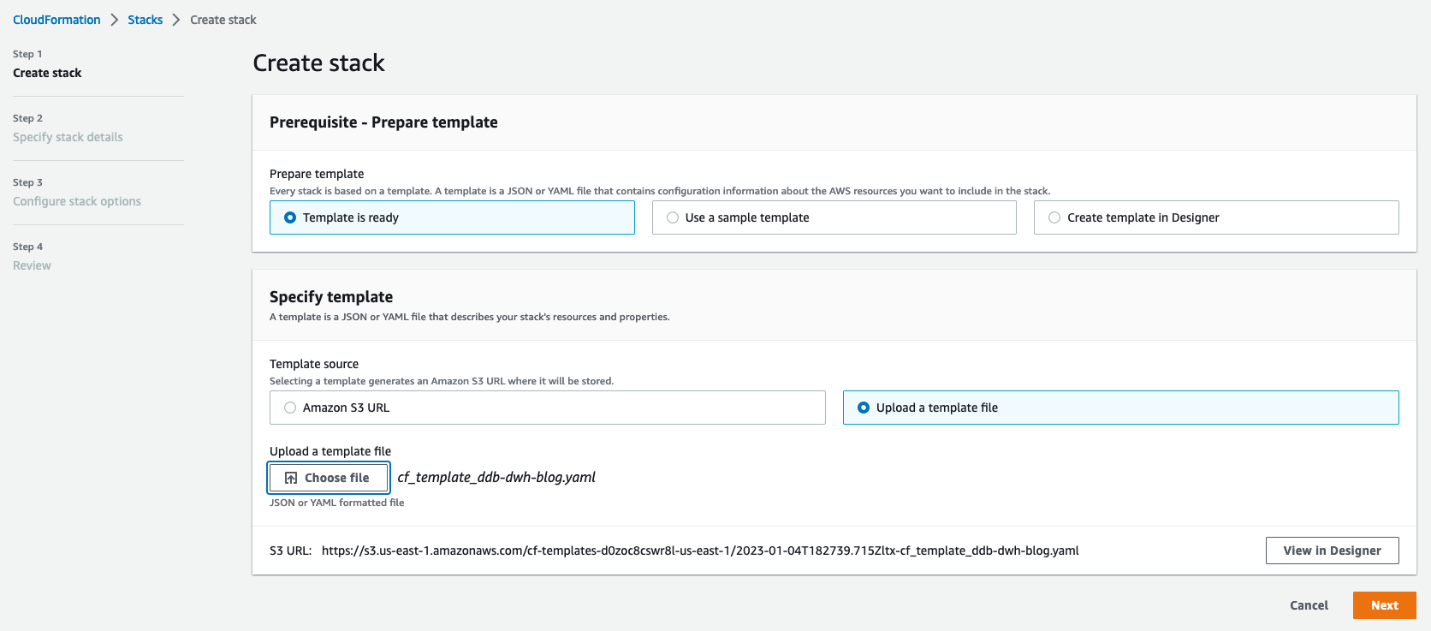
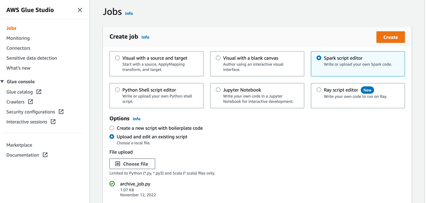
Difference between message Header addresses and Envelope addresses

Before we dive into the use cases, let’s discuss how message addressing works in SES. When a client makes a request, SES constructs an email message compliant with the RFC 5322 Internet Message Format specification . An email comprises of a header, a body, and an RFC 5321 envelope, as described in the Email format in Amazon SES document.

The email addresses in the RFC 5322 To, Cc and Bcc headers are for display. These headers enable your email client interface to display to whom the message was addressed. These addresses do not control which recipients receive the messages; the envelope addresses do. The sending mail client provides the envelope recipient addresses to a mail server using the RFC 5321 RCPT TO commands. RCPT is an abbreviation for recipient.

An apt analogy (see diagram below) is how a physical letter within an envelope can address a person whose address is not the envelope. The address on the envelope is what the mail carrier to deliver the envelope. The postal worker should not need to open the envelope to know which address to deliver the mail.

Analogy to show physical mail compares to electronic mail

As an example, a school district may send letters informing residents of enrollment details for their children, but they do not know all of the names of the people who live at each address. The envelope may only list the address, and the letter may just be addressed “To Resident” if the school district doesn’t have a name to address the letter. The message is delivered to the resident’s address regardless of the accuracy of the information on the letter.

To simplify, let’s summarize the differences between To & Cc header and envelope addresses:

Header To & Cc Addresses Envelope Addresses (RCPT)
Used by email clients to display the list of recipients Used by mail servers to deliver the email message
Not used for mail delivery Used for mail delivery
Displayed to recipients Not displayed to recipients

The Bcc address is different than the To and Cc headers because it is used to send a copy of the message to an additional set of recipients that are “blind” to the other recipients. Bcc addresses are only defined by envelope addresses, not as a header address. Mail servers will commonly remove a Bcc header when handling a message, but delivery to the envelope recipient address still occurs.

When to use multiple recipients in a Destination

SES supports sending messages to multiple recipients in a single SendEmail operation. The Destination argument of the SendEmail operation represents the destination of the message. A Destination consists of To, Cc, and Bcc fields which represent both the header addresses and the envelope addresses.

When multiple recipients are defined in the Destination argument to the SendEmail operation, the defining characteristic is that every recipient receives the exact same message with the same message-id. A message-id is used for event handling (bounces, complaints, etc) among other purposes. A message-id pertains to exactly one version of a particular message.

Did you know: The use cases for recipients having a message with the same message-id are limited to situations in which the recipients are expected to interact with the message as a group. For example, recipients may reply-all to the email and have a resulting email conversation. The original message-id is used by email client applications to display a “conversation” view using the References and In-Reply-To headers. This behavior may be a good fit if the use case is a mailing list or internal announcement to employees within a company.

The recipient limit in the Destination argument is 50 because that is a reasonable break-point when the “conversational” use case runs the risk of the “reply all storm“ described in the next section. Consider using a robust mailing list solution or hosted service with capabilities similar to GNU Mailman to facilitate large group email conversations.

Why bulk mail recipients should not see other recipients

For bulk sending purposes, and most transactional sending, the recipients don’t need to know that other recipients also received the message:

  • The recipients likely gain no value from seeing the other recipient addresses, as they may be arbitrarily segmented into batches of 50 or less, and most email client interfaces have trouble displaying more than 50 addresses.
  • There is a risk of a “reply-all storm“, which is when a recipient replies to all of the To and Cc addresses from the original message, and then those people reply back asking everyone to stop replying. This scenario is fun to talk about around the water cooler, but should be avoided.
  • If recipients are defined as Bcc recipients in the Destinations argument of the SendEmail operation, it would not contain a To address, and that can look suspicious when read by the recipients.

Note: There is no authentication mechanism protecting the To or Cc headers from spoofing, so be careful about assuming any trust placed into the values of those headers. This means that it is possible for an attacker to spoof the To or Cc headers in an email message. Therefor the only meaningful address to include in the To header is the recipient’s own address, which they know isn’t spoofed because of the fact that they are reading the message.

For bulk mail it is best practice to have each recipient see only their own name and email address in the To header of the messages they receive. This makes the messages look more personable and can improve deliverability and recipient engagement.

This approach can be achieved by sending the message to each recipient individually via the SendEmail operation. You would use a single address in the “ToAddressses” field of the “Destination” argument.

Use the ToAddress field to individual message in the SendEmail API

How email event notifications are associated with recipients

If you need email event notifications to be associated to each recipient, then you will need each recipient to receive a message with a unique message-id; one recipient per Destination.

The following event types will be associated with every recipient in the Destination:

  • asynchronous bounces
  • complaints
  • opens
  • clicks

Learn more about Amazon SES events in the documentation: how email sending works in Amazon SES

For example, if one of the recipients triggers a open engagement event, and if that recipient was in a group of 50 recipients within the Destination argument to the SendEmail operation, then all 50 of those recipients will be registered as having opened the message.

Other considerations:

  • If the recipients are defined by ToAddresses and CcAddresses they will all appear in the message headers, but the To and Cc headers will be truncated in the event notifications if the headers are over 10 KB. Multi-recipient Destinations may cause you to lose observability needed to troubleshoot deliverability issues.
  • SES Virtual Deliverability Manager only tracks metrics from emails that have one recipient. Multi-recipient Destinations are not counted in any of the Virtual Deliverability Manager dashboard metrics.
  • SES counts the number of envelope recipients in an email toward the account’s sending quotas. Multi-recipient Destinations is not a way to achieve higher sending limits.
  • SES charges for each recipient receiving a message regardless of how many recipients are included in the Destination for each API invocation. Multi-recipient Destinations is not a way to reduce costs.

For bulk sending use cases, it is best practice to have each recipient have a copy of the message with a unique message-id to achieve the highest level of observability of your email sending program. High observability leads to high deliverability. This can be achieved by sending the message to each recipient individually.

How to send Emails to multiple recipients with SES

At this point, you should understand why it is a best practice to send a message to multiple recipients by iteratively using a single recipient in the Destination argument of the SendEmail operation.

Sending a message to a single recipient at a time is the best way to get started delivering messages to multiple recipients. Sending email in this fashion ensures that your deliverability metrics are giving you the observability needed to achieve the highest engagement with your recipients.

The following example uses the SES version 2 command line interface (CLI) to send a message to a list of recipients. If you do not want to use the CLI, use SES with an AWS SDK and adapt the commands into the syntax of the SDK of your choice.

#!/bin/bash

# Replace these variables with your own values
# sender 
# - Consider not using no-reply@, and instead use SES Inbound to receive replies
# - Consider a descriptive username@; some mobile clients will display it prominently, so it should make sense to the recipient.
# - Consider using a subdomain for bulk and transactional mail. Don't use the domain used by your users.
# - Consider using a verified domain identity. Don't use an email address identity within a domain that has a DMARC policy.
sender="[email protected]"
subject="Email subject"
body="Email body"
region="us-east-1"

# List of recipients, one per line. Defaults to SES mailbox simulator addresses (https://docs.aws.amazon.com/ses/latest/dg/send-an-email-from-console.html#send-email-simulator-how-to-use)
recipients=(
  "[email protected]"
# ... 
  "[email protected]"
)

# Send an email to each recipient
# Iterate through the list of recipients.
# Invoke the AWS SES SendEmail operation with a single recipient defined in the Destination
for recipient in "${recipients[@]}"; do
  aws sesv2 send-email \
    --from-email-address "$sender" \
    --destination "ToAddresses=$recipient" \
    --content "Simple={Subject={Data='$subject',Charset='UTF-8'},Body={Text={Data='$body',Charset='UTF-8'}}}" \
    --region "$region"
done

# The output will look similar to this, with a unique MessageID associated with each recipent.
# {
#    "MessageId": "010001874edd1765-be4ea5c2-d2b1-4ffb-bfb9-46461d18d80c-000000"
# }
# ... 51 total message-ids
# {
#    "MessageId": "010001874edd1b94-468ecee9-9198-4356-9f53-a108097777e5-000000"
# }

In this example script, the SendEmail operation is invoked multiple times using the CLI to deliver the message individually to each recipient, and each recipient only sees their own address in the To header. We called the SendEmail operation 51 times and a total of 51 Message Ids were returned in the response.

How to use SendEmail for multiple recipient advanced use cases

Consider a scenario where a memo needs to be sent to an entire team, the team is large, and only a few of the recipients need to be displayed in the headers. In this use case, it is desirable to send multiple copies of an email to many recipients who all receive the same To and Cc headers.

To customize the headers, you must use the Raw field of the Content argument instead of the Simple field.

The example below will reference another internet standard called Multipurpose Internet Mail Extensions (MIME): Format of Internet Message Bodies.

What’s in a MIME object:

  • Headers (such as From, Subject, and Reply-to)
  • Body – Plain text and HTML
  • Attachments – Files and images

MIME extends the capabilities of RFC 5322 and is used to format most email messages to this day. There are a variety of packages that can assist in creating a MIME structured messages, which you can find by searching relevant package managers.

This is an example in Python to create a MIME formatted message for the next script.

#!/usr/bin/env python
from email.mime.multipart import MIMEMultipart
from email.mime.text import MIMEText
import base64

# You must change the 'fromAddress' variable for this example to work in your environment.
#
# When choosing a From header address:
# - Consider not using no-reply@, and instead use SES Inbound to receive replies
# - Consider a descriptive username@; some mobile clients will display it prominently, so it should make sense to the recipient.
# - Consider using a subdomain for bulk and transactional mail. Don't use the domain used by your users.
# - Consider using a verified domain identity. Don't use an email address identity within a domain that has a DMARC policy.

fromAddress = "Descriptive Name <[email protected]>"

# The To and Cc addresses here are for the email header. They are what will be displayed to the recipient.
# The actual recipient, or evelope recipient, will be set later.
toAddresses = ['Founder Name <[email protected]>']
ccAddresses = ['President <[email protected]>', 'Director <[email protected]>']
subjectTxt = "Success and Scale Bring Broad Responsibility"
messageTxt = "We started in a garage, but we’re not there anymore. We are big, we impact the world, and we are far from perfect. We must be humble and thoughtful about even the secondary effects of our actions. Our local communities, planet, and future generations need us to be better every day. We must begin each day with a determination to make better, do better, and be better for our customers, our employees, our partners, and the world at large. And we must end every day knowing we can do even more tomorrow. Leaders create more than they consume and always leave things better than how they found them."
messageHtml = "<html><body><p>" + messageTxt + "</p></body></html>"
CHARSET = "utf-8"

multiPartEmail = MIMEMultipart()
multiPartEmail['From'] = fromAddress
toAddressesJoined = ",".join(toAddresses)
multiPartEmail['To'] = toAddressesJoined
ccAddressesJoined = ",".join(ccAddresses)
multiPartEmail['Cc'] = ccAddressesJoined
multiPartEmail['Subject'] = subjectTxt
msg_body = MIMEMultipart('alternative')
textpart = MIMEText(messageTxt.encode(CHARSET), 'plain', CHARSET)
htmlpart = MIMEText(messageHtml.encode(CHARSET), 'html', CHARSET)
msg_body.attach(textpart)
msg_body.attach(htmlpart)
multiPartEmail.attach(msg_body)

print("Human readable blob:")
print((multiPartEmail.as_string()))
print("Base64 Encoded Blob:")
print(base64.b64encode(multiPartEmail.as_bytes()))
Running this script will produce output similar to the following:
Human readable blob:
Content-Type: multipart/mixed; boundary="===============0865862865556646150=="
MIME-Version: 1.0
From: [email protected]
To: [email protected]
Cc: [email protected], [email protected]
Subject: Success and Scale Bring Broad Responsibility

--===============0865862865556646150==
Content-Type: text/text/plain; charset="us-ascii"
MIME-Version: 1.0
Content-Transfer-Encoding: 7bit

We started in a garage, but we’re not there anymore. We are big, we impact the world, and we are far from perfect. We must be humble and thoughtful about even the secondary effects of our actions. Our local communities, planet, and future generations need us to be better every day. We must begin each day with a determination to make better, do better, and be better for our customers, our employees, our partners, and the world at large. And we must end every day knowing we can do even more tomorrow. Leaders create more than they consume and always leave things better than how they found them.

--===============0865862865556646150==--

Base64 Encoded Blob:
b'Q29udGVudC1U...TRIMMED...'

The following script has an option to divide the list into batches of 50 or fewer for each SendEmail operation and will send a Base 64 encoded MIME object to a list of recipients. The headers of the message are always the same for every recipient because the headers are defined within the MIME object, which is obtained from running the previous script With SendEmail, the Destination argument does not define the To or Cc headers.

#!/bin/bash

# Replace these variables with your own values
region="us-east-1"

# List of recipients, one per line. Defaults to SES mailbox simulator addresses (https://docs.aws.amazon.com/ses/latest/dg/send-an-email-from-console.html#send-email-simulator-how-to-use)
# These are the actual envelope recipients who will get the above email in their inbox. The To and Cc addresses set above will be displayed, not these.
recipients=(
"[email protected]"
# ...
"[email protected]"
)

# Raw message content
# Paste the base64 encoded message blob that is returned from the python script (the string within b'')
content=''

# Maximum number of recipients per batch
# Increase batch_size up to 50 if your use case requires every recipient have the same message-it. This sacrifices observability into deliverability metrics.
batch_size=1

# Send an email to batch size of 1 to 50 recipients
recipients_count=${#recipients[@]}
echo $recipients_count
for ((i=0; i<$recipients_count; i+=batch_size)); do
to_addresses="${recipients[@]:${i}:${batch_size}}"
to_addresses="${to_addresses// /,}"
aws sesv2 send-email \
--destination "ToAddresses=$to_addresses" \
--content "Raw={Data='$content'}" \
--region "$region"
done

# The output will look similar to this, with a unique MessageID associated with each send-email.
#{
# "MessageId": "010001874ee5cdca-3fe4fb4b-4d36-4ae7-b4e4-cc7fae988a42-000000"
#}
#... 51 total message-ids
#{
# "MessageId": "010001874ee5d210-9225f471-e330-4f01-9044-63a941358477-000000"
#}

Screenshot of email client, viewing email sent by the above code. The sender of the email is “Descriptive Name”, the To recipient is Founder Name, and the President and Director are displayed as Cc addresses.

Remember: If you increase the batch size to greater than 1. Every recipient in each batch will have a message with the same message-id and will all be treated the same for event processing.

Running these scripts will have the effect of each team member receiving exactly the same looking message regardless of how many recipients were defined in each SendEmail Destination. The To and CC addresses were set in the email headers, but the actual envelope recipients were set in the API operation.

SES SendEmail and SendBulkEmail APIs

The latest version of SES API (version 2) offers SendEmail and SendBulkEmail APIs.

With SendBulkEmail, you can only use a pre-defined SES template while, with SendEmail, you can send any email format including raw, text, HTML and templates.

SendEmail operation can send a single email to one Destination (50 recipients across the To:, Cc:, and Bc: fields) while the SendBulkEmail operation can send 50 unique emails to 50 Destinations by leveraging a SES template.

Both operations have the capability to send templated emails, but the SendBulkEmail operation requires less computational resources. This is due to its ability to send emails to 50 Destinations using just a single API call.

Conclusion

In this blog post we discussed how message recipient addresses are displayed by email clients, how message delivery is defined by envelope recipients, and how email sending events are associated with the recipients. Defining multiple recipients in a message destination can lead to poor observability and therefore poor deliverability and should not be used unless your use case specifically requires it

Sending messages to one recipient at a time is a best practice and leads to the highest engagement with your recipients.

About the authors

Jesse Thompson is an Email Deliverability Manager with the Amazon Simple Email Service team. His background is in enterprise IT development and operations, with a focus on email abuse mitigation and encouragement of authenticity practices with open standard protocols. Jesse’s favorite activity outside of technology is recreational curling.
Samuel Wallan is a Software Development Engineer at AWS Simple Email Service. Within SES, Sam works on the Digital User Experience Deliverability team. In his free time, he enjoys hanging out with friends and staying fit.
Farnam Farshneshani is a Technical Account Manager at AWS. He specializes in AWS Simple Email service and helps customers with operational and architectural issues.  In his free time, he enjoys traveling and participating in various outdoor activities.
Joydeep Dutta is a Senior Solutions architect at AWS. Joydeep enjoys working with AWS customers to migrate their workloads to the AWS Cloud, optimize for cost and help with architectural best practices. He is passionate about enterprise architecture to help reduce cost and complexity in the enterprise. He lives in New Jersey and enjoys listening to music and spending time in the outdoors in his spare time.

The collective thoughts of the interwebz