Code scanning and Ruby: turning source code into a queryable database

Post Syndicated from Nick Rolfe original https://github.blog/2022-02-01-code-scanning-and-ruby-turning-source-code-into-a-queryable-database/

We recently added beta support for Ruby to the CodeQL engine that powers GitHub code scanning, as part of our efforts to make it easier for developers to build and ship secure code. Ruby support is particularly exciting for us, since GitHub itself is a Ruby on Rails app. Any improvements we or the community make to CodeQL’s vulnerability detection will help secure our own code, in addition to helping Ruby’s open source ecosystem.

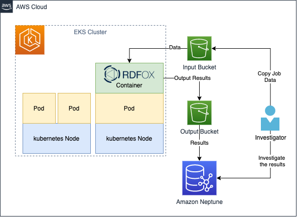
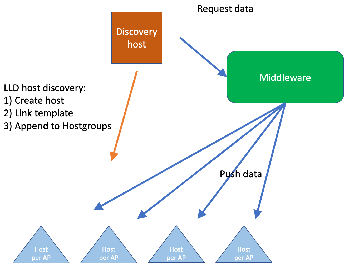
CodeQL’s static analysis works by running queries over a database representation of a program. The following diagram gives a high-level overview of the process:

codeql diagram

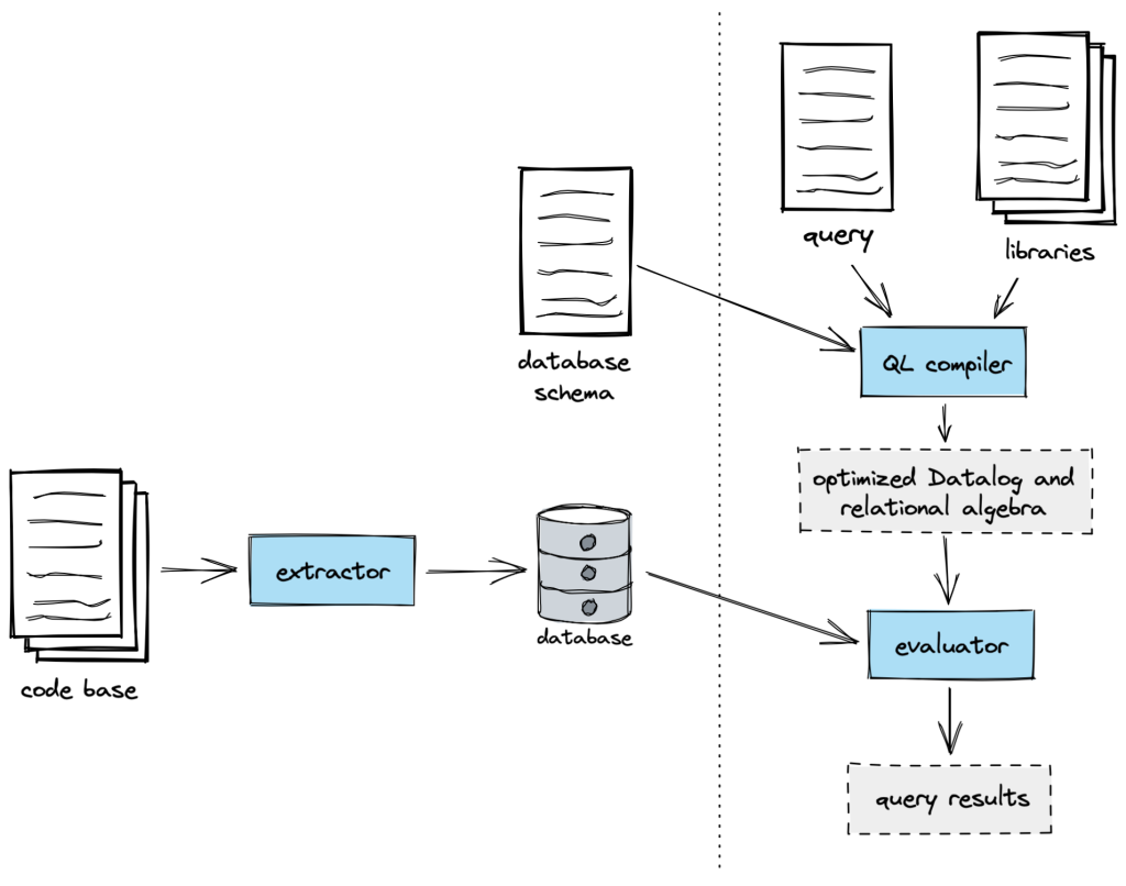
While there’s plenty I’d love to tell you about how we write queries, and about our rich set of analysis libraries, I’m going to focus in this post on how we build those databases: how we’ve typically done it for other languages and how we did things a little differently for Ruby.

Introducing the extractor

If you want to be able to create databases for a new language in CodeQL, you need to write an extractor. An extractor is a tool that:

  1. parses the source code to obtain a parse tree,
  2. converts that parse tree into a relational form, and
  3. writes those relations (database tables) to disk.

You also need to define a schema for the database produced by your extractor. The schema specifies the names of tables in the database and the names and types of columns in each table.

Let’s visit parse trees, parsers, and database schemas in more detail.

Parse trees

Source code is just text. If you’re writing a compiler, performing static analysis, or even just doing syntax highlighting, you want to convert that text to a structure that is easier to work with. The structure we use is a parse tree, also known as a concrete syntax tree.

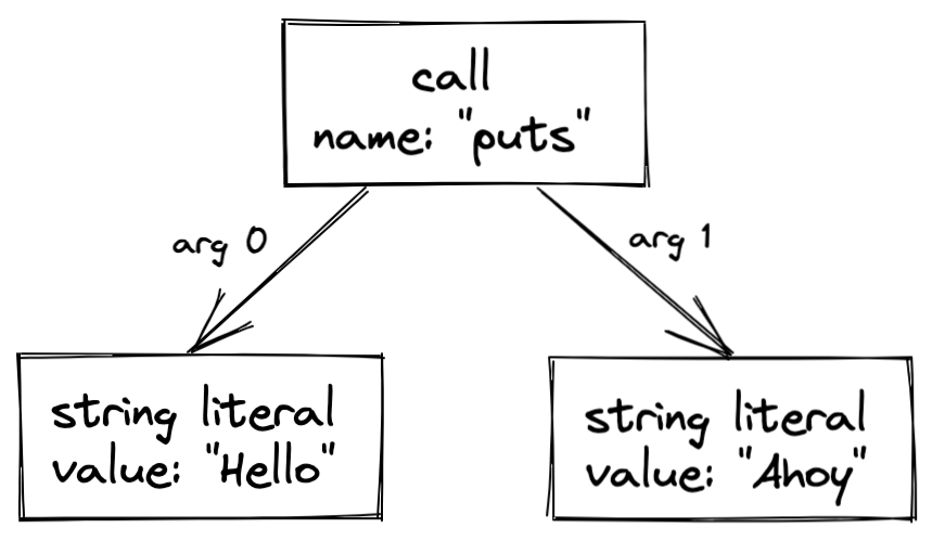
Here’s a friendly little Ruby program that prints a couple of greetings:

puts("Hello", "Ahoy")

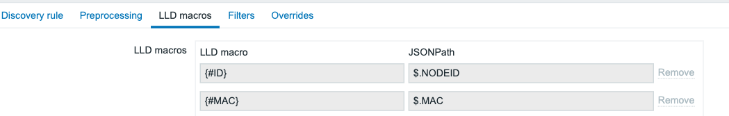
The program contains three expressions: the string literals "Hello" and "Ahoy" and a call to a method named puts. I could draw a minimal parse tree for the program like this:

P

Compilers and static analysis tools like CodeQL often convert the parse tree into a simpler format known as an abstract syntax tree (AST), so-called because it abstracts away some of the syntactic details that do not affect the meaning of the program, such as comments, whitespace, and parentheses. If I wanted – and if I assume that puts is a method built into the language – I could write a simple interpreter that executes the program by walking the AST.

For CodeQL, the Ruby extractor stores the parse tree in the database, since those syntactic details can sometimes be useful. We then provide a query library to transform this into an AST, and most of our queries and query libraries build on top of that transformed AST, either directly or after applying further transformations (such as the construction of a data-flow graph).

Choosing a parser

For each language we’ve supported so far, we’ve used a different parser, choosing the one that gives the best performance and compatibility across all the codebases we want to analyze. For example, our C# extractor parses C# source code using Microsoft’s open source Roslyn compiler, while our JavaScript extractor uses a parser that was derived from the Acorn project.

For Ruby, we decided to use tree-sitter and its Ruby parser. Tree-sitter is a parser framework developed by our friends in GitHub’s Semantic Code Team and is the technology underlying the syntax highlighting and code navigation (jump-to-definition) features on GitHub.com.

Tree-sitter is fast, has excellent error recovery, and provides bindings for several languages (we chose to use the Rust bindings, which are particularly pleasant). It has parsers not only for Ruby, but for most other popular languages, and provides machine-readable descriptions of each language’s grammar. These opened up some exciting possiblities for us, which I’ll describe later.

In practice, the parse tree produced by tree-sitter for our example program is a little more complicated than the diagram above (for one thing, string literal nodes have child nodes in order to support string interpolation). If you’re curious, you can go to the tree-sitter playground, select Ruby from the dropdown, and try it for yourself.

Handling ambiguity

Ruby has a flexible syntax that delights (most of) the people who program in it. The word ‘elegant’ gets thrown around a lot, and Ruby programs often read more like English prose than code. However, this elegance comes at a significant cost: the language is ambiguous in several places, and dealing with it in a parser creates a lot of complexity.

Ruby is simple in appearance, but is very complex inside, just like our human body.

– Yukihiro 'Matz' Matsumoto, Ruby's creator

Matz’s Ruby Interpreter (MRI) is the canonical implementation of the Ruby language, and its parser is implemented in the file parse.y (from which Bison generates the actual parser code). That file is currently 14,000 lines long, which should give you a sense of the complexity involved in parsing Ruby.

One interesting example of Ruby’s ambiguity occurs when parsing an unadorned identifier like foo. If it had parentheses – foo() – we could parse it unambiguously as a method call, but parentheses are optional in Ruby. Is foo a method call with zero arguments, or is it a variable reference? Well, that ultimately depends on whether a variable named foo is in scope. If so, it’s a variable reference; otherwise, we can assume it’s a call to a method named foo.

What type of parse-tree node should the parser return in this case? The parser does not track which variables are in scope, so it cannot decide. The way tree-sitter and the extractor handle this is to emit an identifier node rather than a call node. It’s only later, as we evaluate queries, that our AST library builds a control-flow graph of the program and uses that to decide whether the node is a method call or a variable reference.

Representing a parse tree in a relational database

While the parse trees produced by most parser libraries typically represent nodes and edges in the tree as objects and pointers, CodeQL uses a relational database. Going back to the simple diagram above, I can attempt to convert it to relational form. To do that, I should first define a schema (in a simplified version of CodeQL’s schema syntax):

expressions(id: int, kind: int)
calls(expr_id: int, name: string)
call_arguments(call_id: int, arg_id: int, arg_index: int)
string_literals(expr_id: int, val: string)

The expressions table has a row for each expression in the program. Each one is given a unique id, a primary key that I can use to reference the expression from other tables. The kind column defines what kind of expression it is. I can decide that a value of 1 means the expression is a method call, 2 means it’s a string literal, and so on.

The calls table has a row for each method call, and it allows me to specify data that is specific to call expressions. The first column is a foreign key, i.e. the id of the corresponding entry in the expressions table, while the second column specifies the name of the method. You might have expected that I’d add columns for the call’s arguments, but calls can take any number of arguments, so I wouldn’t know how many columns to add. Instead, I put them in a separate call_arguments table.

The call_arguments table, therefore, has one row per argument in the program. It has three columns: one that’s a reference to the call expression, another that’s a reference to an argument, and a third that specifies the index, or number, of that argument.

Finally, the string_literals table lets me associate the literal text value with the corresponding entry in the expressions table.

Populating our small database

Now that I’ve defined my schema, I’m going to manually populate a matching database with rows for my little greeting program:

expressions

id kind
100 1 (call)
101 2 (string literal)
102 2 (string literal)

calls

expr_id name
100 “puts”

call_arguments

call_id arg_id arg_index
100 101 0
100 102 1

string_literals

expr_id val
101 “Hello”
102 “Ahoy”

Suppose this were a SQL database, and I wanted to write a query to find all the expressions that are arguments in calls to the puts method. It might look like this:

SELECT call_arguments.arg_id
FROM call_arguments
INNER JOIN calls ON calls.expr_id = call_arguments.call_id
WHERE calls.name = "puts";

In practice, we don’t use SQL. Instead, CodeQL queries are written in the QL language and evaluated using our custom database engine. QL is an object-oriented, declarative logic-programming language that is superficially similar to SQL but based on Datalog. Here’s what the same query might look like in QL:

from MethodCall call, Expr arg
where
  call.getMethodName() = "puts" and
  arg = call.getAnArgument()
select arg

MethodCall and Expr are classes that wrap the database tables, providing a high-level, object-oriented interface, with helpful predicates like getMethodName() and getAnArgument().

Language-specific schemas

The toy database schema I defined might look as though it could be reused for just about every programming language that has string literals and method calls. However, in practice, I’d need to extend it to support some features that are unique to Ruby, such as the optional blocks that can be passed with every method call.

Every language has these unique quirks, so each one GitHub supports has its own schema, perfectly tuned to match that language’s syntax. Whereas my toy schema had only two kinds of expression, our JavaScript and C/C++ schemas, for example, both define over 100 kinds of expression. Those schemas were written manually, being refined and expanded over the years as we made improvements and added support for new language features.

In contrast, one of the major differences in how we approached Ruby is that we decided to generate the database schema automatically. I mentioned earlier that tree-sitter provides a machine-readable description of its grammar. This is a file called node-types.json, and it provides information about all the nodes tree-sitter can return after parsing a Ruby program. It defines, for example, a type of node named binary, representing binary operation expressions, with fields named left, operator, and right, each with their own type information. It turns out this is exactly the kind of information we want in our database schema, so we built a tool to read node-types.json and spit out a CodeQL database schema.

You can see the schema it produces for Ruby here.

Bridging the gap

I’ve talked about how the parser gives us a parse tree, and how we could represent that same tree in a database. That’s really the main job of an extractor – massaging the parse tree into a relational database format. How easy or difficult that is depends a lot on how similar those two structures look. For some languages, we defined our database schema to closely match the structure (and naming scheme) of the tree produced by the parser. That is, there’s a high level of correspondence between the parser’s node names and the database’s table names. For those languages, an extractor’s job is fairly simple. For other languages, where we perhaps decided that the tree produced by the parser didn’t map nicely to our ideal database schema, we have to do more work to convert from one to the other.

For Ruby, where we wrote a schema-generator to automatically translate tree-sitter’s description of its node types, our extractor’s job is quite simple: when tree-sitter parses the program and gives us those tree nodes, we can perform the same translations and automatically produce a database that conforms to the schema.

Language independence

This extraction process is not only straightforward, it’s also completely language-agnostic. That is, the process is entirely mechanical and works for any tree-sitter grammar. Our schema-generator and extractor know nothing about Ruby or its syntax – they simply know how to translate tree-sitter’s node-types.json. Since tree-sitter has parsers for dozens of languages, and they all have corresponding node-types.json files, we have effectively written a pair of tools that could produce CodeQL databases for any of them.

One early benefit of this approach came when we realized that, to provide comprehensive analysis of Ruby on Rails applications, we’d also need to parse the ERB templates used to render Rails views. ERB is a distinct language that needs to be parsed separately and extracted into our database. Thankfully, tree-sitter has an existing ERB parser, so we simply had to point our tooling at that node-types.json file as well, and suddenly we had a schema-generator and extractor that could handle both Ruby and ERB.

As an aside, the ERB language is quite simple, mostly consisting of tags that differentiate between the parts of the template that are text and the parts that are Ruby code. The ERB parser only cares about those tags and doesn’t parse the Ruby code itself. This is because tree-sitter provides an elegant feature that will return a series of byte offsets delimiting the parts that are Ruby code, which we can then pass on to the Ruby parser. So, when we extract an ERB file, we parse and extract the ERB parse tree first, and then perform a second pass that parses and extracts the Ruby parse tree, ignoring the text parts of the template file.

Of course, this automated approach to extraction does come with some tradeoffs, since it involves deferring some work from the extraction stage to the analysis stage. Our QL AST library, for example, has to do more work to transform the parse tree into a user-friendly AST representation, compared with some languages where the AST classes are thin wrappers over database tables. And if we look at our existing extractor for C#, for example, we see that it gets type information from the Roslyn compiler frontend, and stores it in the database. Our language-independent tooling, meanwhile, does not attempt any kind of type analysis, so if we wanted to use it on a static language, we’d have to implement that type analysis ourselves in QL.

Nonetheless, we are excited about the possibilities this language-independent tooling opens up as we look to expand CodeQL analysis to cover more languages in the future, especially for dynamic languages. There’s a lot more to analyzing a language than producing a database, but getting that part working with little to no effort should be a major time-saver.

github/github: so good, they named it twice

github/github is the Ruby on Rails application that powers GitHub.com, and it’s rather large. I’ve heard it said that it’s one of the largest Rails apps in the world. That means it’s an excellent stress test for our Ruby extractor.

It was actually the second Ruby program we ever extracted (the first was “Hello, World!”).

Of course, extraction wasn’t quite perfect. We observed a number of parser errors that we fixed upstream in the tree-sitter-ruby project, so our work not only resulted in improved Ruby code-viewing on GitHub.com, but also improvements in the other projects that use tree-sitter, such as Neovim’s syntax highlighting.

It was also a useful benchmark in our goal of making extraction as fast as possible. CodeQL can’t start doing the valuable work of analyzing for vulnerabilities until the code has been extracted and a database produced, so we wanted to make this as fast as possible. It certainly helps that tree-sitter itself is fast, and that our automatic translation of tree-sitter’s parse tree is simple.

The biggest speedup – and where our choice to implement the extractor in Rust really helped – was in implementing multi-threaded extraction. With the design we chose for the Ruby extractor, the work it performs on each source file is completely independent of any other source file. That makes extraction an embarrassingly parallel problem, and using the Rayon library meant we barely had to change any code at all to take advantage of that. We simply changed a for loop to use a Rayon parallel-iterator, and it handled the rest. Suddenly extraction got eight times faster on my eight-core laptop.

CodeQL now runs on every pull request against github/github, using a 32-core Actions runner, where Ruby extraction takes just 15 seconds. The core engine still has to perform ‘database finalization’ after the extractor finishes, and this takes a little longer (it parallelizes, but not “embarrassingly”), but we are extremely pleased with the extractor’s performance given the size of the github/github codebase, and given our experiences with extracting other languages.

We should be in a good place to accommodate all our users’ Ruby codebases, large and small.

Try it out

I hope you’ve enjoyed this dive into the technical details of extracting CodeQL databases. If you’d like to try CodeQL on your Ruby projects, please refer to the blog post announcing the Ruby public beta, which contains several handy links to help you get started.

Financial Crime Discovery using Amazon EKS and Graph Databases

Post Syndicated from Severin Gassauer-Fleissner original https://aws.amazon.com/blogs/architecture/financial-crime-discovery-using-amazon-eks-and-graph-databases/

Discovering and solving financial crimes has become a challenge due to an increasing amount of financial data. While storing transactional payment data in a structured table format is useful for searching, filtering, and calculations, it is not always an ideal way to represent transactional data. For example, determining if there is a suspicious financial relationship between entity A and entity B is difficult to visualize in a table. Using tables, we would have to do SQL joins for every possible transaction from entity A to every possible subsequent transaction. We would then have to iterate this process until we found a relationship to entity B. Moreover, certain queries are challenging to run on a relational database management system (RDBMS). For example, it can be quite time consuming to discover which account received a minimum amount of $10,000,000 from other accounts.

Graph databases such as Amazon Neptune can be helpful with performing queries, because they can traverse the data and perform calculations simultaneously. Graphs enable us to represent transactions and parties over a multi-connected network, and discover patterns and chains of connections. It is common to use them in anti-money laundering (AML) applications, as they can help find patterns of suspicious transactions.

We needed a solution that could scale and process millions of transactions, by effectively using high memory and CPU configurations to perform complex queries quickly. As part of our customer demonstration to show how graph databases can help discover financial crimes, we also sourced a large dataset on which to test the solution. We used a graph database, Amazon Elastic Kubernetes Service (EKS), and Amazon Neptune, to search for suspicious financial chains across large amounts of transactional data in minutes.

Overview of our conceptual financial crime discovery solution

Figure 1. Workflow for financial crime discovery

Figure 1. Workflow for financial crime discovery

We first needed to find a rules engine that could perform transaction inferencing and reasoning. It had to be able to process various rules on our data, be efficient, and able to scale. Next, we needed a straightforward way to ingest data into the solution. Once we had the data available, we needed to initiate a task to begin our inference job. Finally, we needed a location to store the result for further analysis and persistence, see Figure 1.

Using the AWS Cloud to scale up a graph database

We used multiple AWS services to create a fully automated end-to-end batch-based transaction process, shown in Figure 2. We used RDFox, which is an AWS Marketplace product, created by Oxford Semantic Technologies. RDFox is a high-performance in-memory graph database and semantic reasoner. To orchestrate RDFox, we used Amazon EKS Autoscaler to spin up a cluster to instantiate the RDFox container. Amazon EKS can spin up multiple containers for difference inference jobs and recycle the resources when the job finishes. We also used Amazon Neptune, an Amazon managed distributed graph database that can store up to 64 TiB of the results for diagnosis and long-term retention.

The data is stored in Amazon S3 buckets, which provide a streamlined way to feed a large dataset for processing.

Figure 2. Architecture diagram for financial crime discovery

Figure 2. Architecture diagram for financial crime discovery

Financial crimes rules

The power of graphs can help discover financial crimes that are reflected in relationships and monetary transactions. To demonstrate this, we will write two rules to detect two scenarios:

  1. Given two suspicious parties X and Y, find out if there is a transactional relationship between them, and if so, provide the chain that connects them. This is a common scenario that financial institutions must detect.
  2. Given a chain identifying suspicious behavior, find out if the minimum transaction amount that reached the beneficiary exceeds a threshold of Z dollars.

Generating data

To generate data for testing, we used a synthetic data generator written in Python (see GitHub repo in References). The generator built two sets of graph artifacts – parties and transactions. Every transaction is being paired with two random parties, and this iterative process creates a network of connected transactions and parties.

We created a dataset with a small percentage (0.01%) of parties tagged as “Suspicious Party,” to simulate the preceding business scenario. Note that those parties will have transactions going both in and out. In some cases, this will collide with other suspicious parties and establish a chain. This method enables us to get simulated data without engineering the suspicious chains.
The test dataset used with this solution comprises 1M transactions and thousands of parties.
For more information on generating data, see GitHub: Transaction Chains Data Generator.

Walkthrough of the financial investigator workflow

Once deployed, this solution can assist investigators as follows:

  1. An investigator places the transactions and party data (nt triples) in a subdirectory within the input bucket. Typically, subdirectories can be named as a date or range of dates. In addition, the investigator uploads the particular rules (dlog files) and queries (rq files) that must be processed on the data.
  2. Once the data is ready, the investigator uploads a job spec file (simple JSON, see References section). This contains the description of what resources the job requires (CPUs and memory), along with other configurations for the job.
  3. Once the job spec has been uploaded to the bucket’s subdirectory, the job is automatically initiated. The Kubernetes scheduler will allocate enough resources to initiate the RDFox pod. The containers in the pod will then load, process, query results, and upload them to the output bucket.
  4. Once the data reaches the output bucket, an AWS Lambda function is initiated. This invokes the Amazon Neptune Bulk Loader, which asynchronously loads the results to the Neptune cluster in a parallelized manner.
  5. Once the load completes, the investigator gets an email notification that the job has been completed, and the results are ready for view.

Additionally:

  • The investigator can upload multiple rules and queries, they will all be processed automatically.
  • The investigator can launch multiple jobs with different/same data, and with different rules and queries at the same time.
  • All jobs outputs are saved in a unique job ID subdirectory in the output bucket.

To create the solution in your account, follow the instruction here: GitHub repo

Prerequisites

For this walkthrough, you should have the following prerequisites:

Rules

We create two materialization rule sets to fetch the two scenarios described.

1. detect-suspicious-parties-pair.dlog

The purpose of this first set of rules is to detect chains that might exist between two suspicious parties. The idea of these chains is to represent all the possible relationships that contain monetary transfers between a suspicious originator and the beneficiary. This will include non-suspicious parties in the chain. The rule tags these chains with the “SuspiciousChain” flag.

2. detect-chains-exceed-100-dollars.dlog

This set of rules is designed to tag the chains identified by the first set of rules. It also contains a minimum amount of $100 passed to the beneficiary. We can change the amount to check for different compliance requirements. We tag those chains as “HighValueChain.”

Run the job and check your results

Now we can run our job, with the given data, rules, and two additional queries (to extract “SuspiciousChain” and “HighValueChain” respectively). The result of the queries will be loaded to Amazon Neptune automatically for persistent storage, and is made durably available for further analysis.

Let’s look at the results. The following query can be initiated against RDFox console or Amazon Neptune.

Visualization

PREFIX : <http://oxfordsemantic.tech/transactions/entities#>

PREFIX prop: <http://oxfordsemantic.tech/transactions/properties#>

PREFIX type: <http://oxfordsemantic.tech/transactions/classes#>

PREFIX tt: <http://oxfordsemantic.tech/transactions/tupletables#>

SELECT ?S ?P ?O WHERE {

            ?S a type:SuspiciousChain .

            ?S ?P ?O .

}

Figure 3. Visualizing suspicious chains

Figure 3. Visualizing suspicious chains

Whoa! Figure 3 might look complicated at first, but this is because we are visualizing every pair of suspicious parties that have a relationship with another suspicious party. Let’s filter the query to look only at a single particular chain, which exceeds a minimum of $100 to the beneficiary. The following query can be executed against RDFox console or Amazon Neptune.

PREFIX : <http://oxfordsemantic.tech/transactions/entities#>
PREFIX prop: <http://oxfordsemantic.tech/transactions/properties#>
PREFIX type: <http://oxfordsemantic.tech/transactions/classes#>
PREFIX tt: <http://oxfordsemantic.tech/transactions/tupletables#>

SELECT * WHERE {
?S ?P ?O
{
SELECT ?S WHERE {
?S a type:HighValueChain .

} Limit 1

}

Figure 4. Visualizing a particular chain

Figure 4. Visualizing a particular chain

In Figure 4, we can see that Allison, the suspicious originator of the chain, has sent a transaction to Troy. Troy, who is not suspicious, sent the transaction to Karina. Karina is the suspicious beneficiary. We can also see additional information, such as the transaction amount that Karina received, and the chain length of 2 in this case.

In our testing, we were able to scale up to 500M transactions with 50M parties and process this in less than two hours! And we performed this at a significant lower cost when compared to running constant, fixed similar hardware.

Cleaning up

Follow Terraform cleanup instructions.

Conclusion

Graph databases are a powerful tool to apply reasoning on complex financial relationships. The combination of Amazon Web Services and the RDFox engine results in an automated, scalable, and cost-effective, thanks to the dynamic Kubernetes Cluster Autoscaler. Customers can use this solution and provide their investigators with a tool they can experiment and reason on financial transactions. This solution simplifies the process, and makes it easier to try different rules and queries on complex large data collections.

This blog post is written with Oxford Semantic.

Oxford Semantic Logo

References

Solution:

Further reading

RDFox:

Other:

Backblaze Drive Stats for 2021

Post Syndicated from original https://www.backblaze.com/blog/backblaze-drive-stats-for-2021/

In 2021, Backblaze added 40,460 hard drives and as of December 31, 2021, we had 206,928 drives under management. Of that number, there were 3,760 boot drives and 203,168 data drives. This report will focus on our data drives. We will review the hard drive failure rates for 2021, compare those rates to previous years, and present the lifetime failure statistics for all the hard drive models active in our data center as of the end of 2021. Along the way, we share our observations and insights on the data presented and, as always, we look forward to you doing the same in the comments section at the end of the post.

2021 Hard Drive Failure Rates

At the end of 2021, Backblaze was monitoring 203,168 hard drives used to store data. For our evaluation, we removed 409 drives from consideration which were used for either testing purposes or drive models for which we did not have at least 60 drives. This leaves us with 202,759 hard drives to analyze for this report.

Observations and Notes

The Old Guy Rules: For 2021, the 6TB Seagate (model: ST6000DX000) had the lowest failure rate of any drive model, clocking in with an annualized failure rate (AFR) of 0.11%. This is even more impressive when you consider that this 6TB drive model is the oldest in the fleet with an average age of 80.4 months. The number of drives, 886, and 2021 drive days, 323,390, are on the lower side, but after nearly seven years in operation, these drives are thumbing their nose at the tail end of the bathtub curve.

The Kids Are Alright: Two drive models are new for 2021 and both are performing well. The 16TB WDC drive cohort (model: WUH721816ALE6L0) has an average age of 5.06 months and an AFR of 0.14%. While the 16TB Toshiba drive cohort (model: MG08ACA16TE) has an average age of 3.57 months and an AFR of 0.91%. In both cases, the number of drive days is on the lower side, but these two drive models are off to a good start.

AFR, What Does That Mean?

AFR stands for annualized failure rate. This is different from an annual failure rate in which the number of drives is the same for each model (cohort) throughout the annual period. In our environment, drives are added and leave throughout the year. For example, a new drive installed in Q4 might contribute just 43 days, while a drive that failed in July might contribute 186 days, while drives in continuous operation for the year could contribute 365 days each. We count the number of drive days each drive contributes throughout the period and annualize the total using this formula:

AFR = (drive failures / (drive days / 365)) * 100

The Patient Is Stable: Last quarter, we reported on the state of our 14TB Seagate drives (model: ST14000NM0138) provisioned in Dell storage servers. They were failing at a higher than expected rate and everyone—Backblaze, Seagate, and Dell—wanted to know why. The failed drives were examined by fault analysis specialists and in late Q3 it was decided as a first step to upgrade the firmware for that cohort of drives still in service. The results were that the quarterly failure rate dropped from 6.29% in Q3 to 4.66% in Q4, stabilizing the rapid rise in failures we’d seen in Q2 and Q3. The 19 drives that failed in Q4 were shipped off for further analysis. We’ll continue to follow this process over the coming quarters.

The AFR for 2021 for all drive models was 1.01%, which was slightly higher than the 0.93% we reported for 2020. The next section will compare the data from the last three years.

Comparing Drive Stats for 2019, 2020, and 2021

The chart below compares the AFR for each of the last three years. The data for each year is inclusive of that year only and for the active drive models present at the end of each year.

Digging a little deeper, we can aggregate the different drive models by manufacturer to see how failure rates per manufacturer have fared over the last three years.

Note that for the WDC data, a blank value means we did not have any countable WDC drives in our data center in that quarter.

Trends for 2021

The AFR Stayed Low in 2021: In 2021, the AFR for all drives was 1.01%. This was slightly higher than 2020 at 0.93%, but a good sign that the drop in 2020 from 1.83% in 2019 was not an anomaly. What’s behind the 1.01% for 2021? Large drives, as seen below:

The AFR for larger drives, defined here as 12TB, 14TB, and 16TB drives, are all below the 2021 AFR of 1.01% for all drives. The larger drives make up 69% of the total drive population, but more importantly, they total 66% of the drive days total, while only producing 57% of the drive failures.

The larger drives are also the newer drives, which tend to fail less versus older drives. In fact, the oldest large drive has an average age 33 months, while the youngest “small” (4TB, 6TB, 8TB, and 10TB) drive has an average age of 44.9 months.

In summary, the lower AFR for the larger drives is a major influence in keeping the overall AFR for 2021 low.

Drive Model Diversity Continues: In 2021, we added two new drive models to our farm with no models retired. We now have a total of 24 different drive models in operation. That’s up from a low point of 14 in 2019 and 22 in 2020. The chart below for “Backblaze Quarterly Hard Drive Population Percentage by Manufacturer” examines the changing complexion of our drive farm as we look at the number of models from each manufacturer we used over the past six years.

When we first started, we often mixed and matched drive models, mostly out of financial necessity—we bought what we could afford. As we grew, we bought and deployed drives in larger lots and drive homogeneity settled in. Over the past few years, we have gotten more comfortable with mixing and matching again, enabled by our Backblaze Vault architecture. A Vault is composed of sixty tomes, with each tome being 20 drives. We make each tome the same drive model, but each of the tomes within a vault can have different drive models, and even different drive sizes. This allows us to be less reliant on any particular drive model, so the more drive models the better.

Drive Vendor Diversity Continues, Too: When looking at the chart above for “Backblaze Hard Drive Population by Model Count per Manufacturer Over Time,” you might guess that we have increased the percentage of Seagate drives over the last couple of years. Let’s see if that’s true.

It appears the opposite is true, we have lowered the percentage of Seagate drives in our data centers, even though we have added additional Seagate models.

Why is it important to diversify across multiple manufacturers? Flexibility, just like increasing the number of models. Having relationships with all the primary hard drive vendors gives us the opportunity to get the resources we need in a timely fashion. The fact that we can utilize any one of several different models from these vendors adds to that flexibility.

Lifetime Hard Drive Stats

The chart below shows the lifetime annualized failure rates of all the drive models in production as of December 31, 2021.

Observations and Caveats

The lifetime AFR for all the drives listed above is 1.4% and continues to go down year over year. At the end of 2020, the AFR was 1.54% and at the end of 2019, the AFR stood at 1.62%.

When looking at the chart above, several of the drives have a fairly wide confidence interval (>0.5). In these cases, we do not really have enough information about the drive’s performance to be reasonably confident (>95%) in the AFR listed. This is typically the case with lower drive counts or newer drives.

Looking for SSD Numbers?

We’ll be covering our annual failure rates for our SSD drives in a separate post in the next few weeks. We realized that combining the analysis of our data drives and our boot drives in one post was confusing. Stay tuned.

The Hard Drive Stats Data

The complete data set used to create the information used in this review is available on our Hard Drive Test Data page. You can download and use this data for free for your own purpose. All we ask are three things: 1) you cite Backblaze as the source if you use the data, 2) you accept that you are solely responsible for how you use the data, and 3) you do not sell this data to anyone; it is free.

If you just want the summarized data used to create the tables and charts in this blog post, you can download the ZIP file containing the CSV files for each chart.

Good luck and let us know if you find anything interesting.

The post Backblaze Drive Stats for 2021 appeared first on Backblaze Blog | Cloud Storage & Cloud Backup.

Security updates for Tuesday

Post Syndicated from original https://lwn.net/Articles/883423/rss

Security updates have been issued by Debian (ipython), Fedora (kernel and usbview), Gentoo (webkit-gtk), Oracle (java-1.8.0-openjdk), Red Hat (kpatch-patch and samba), Scientific Linux (samba), Slackware (kernel), SUSE (kernel and samba), and Ubuntu (samba).

Demystifying Interviewing for Backend Engineers @ Netflix

Post Syndicated from Netflix Technology Blog original https://netflixtechblog.com/demystifying-interviewing-for-backend-engineers-netflix-aceb26a83495

By Karen Casella, Director of Engineering, Access & Identity Management

Have you ever experienced one of the following scenarios while looking for your next role?

  • You study and practice coding interview problems for hours/days/weeks/months, only to be asked to merge two sorted lists.
  • You apply for multiple roles at the same company and proceed through the interview process with each hiring team separately, despite the fact that there is tremendous overlap in the roles.
  • You go through the interview process, do really well, get really excited about the company and the people you meet, and in the end, you are “matched” to a role that does not excite you, working with a manager and team you have not even met during the interview process.

Interviewing can be a daunting endeavor and how companies, and teams, approach the process varies greatly. We hope that by demystifying the process, you will feel more informed and confident about your interview experience.

Backend Engineering Interview Loop

When you apply for a backend engineering role at Netflix, or if one of our recruiters or hiring managers find your LinkedIn profile interesting, a recruiter or hiring manager reviews your technical background and experience to see if your experience is aligned with our requirements. If so, we invite you to begin the interview process.

Most backend engineering teams follow a process very similar to what is shown below. While this is a relatively stream-lined process, it is not as efficient if a candidate is interested in or qualified for multiple roles within the organization.

Following is a brief description of each of these stages.

Recruiter Phone Screen: A member of our talent team contacts you to explain the process and to assess high-level qualifications . The recruiter also reviews the relevant open roles to see if you have a strong affinity for one or another. If your interests and experience align well with one or more of the roles, they schedule a phone screen with one of the hiring managers.

Manager Phone Screen: The purpose of this discussion is to get a sense for your technical background, your approach to problem solving, and how you work. It’s also a great opportunity for you to learn more about the available roles, the technical challenges the teams are facing and what it’s like to work on a backend engineering team at Netflix.

Technical Screen: The final screen before on-site interviews is used to assess your technical skills and match for the team. For many roles, you will be given a choice between a take-home coding exercise or a one-hour discussion with one of the engineers from the team. The problems you are asked to solve are related to the work of the team.

Round 1 Interviews: If you are invited on-site, the first round interview is with four or five people for 45 minutes each. The interview panel consists of two or three engineers, a hiring manager and a recruiter. The engineers assess your technical skills by asking you to solve various design and coding problems. These questions reflect actual challenges that our teams face.

Round 2 Interviews: You meet with two or three additional people, for 45 minutes each. The interview panel comprises an engineering director, a partner engineer or manager, and another engineering leader. The focus of this round is to assess how well you partner with other teams and your non-technical skills.

Decision & Offer: After round 2, we review the feedback and decide whether or not we will be offering you a role. If so, you will work with the recruiter to discuss compensation expectations, answer any questions that remain for you, and discuss a start date with your new team.

Enter Centralized Hiring

Some Netflix backend engineering teams, seeking stunning colleagues with similar backgrounds and talents, are joining forces and adopting a centralized hiring model. Centralized hiring is an approach of making multiple hiring decisions through one unified hiring process across multiple teams with shared needs in skill, function and experience level.

The interview approach does not vary much from what is shown above, with one big exception: there are several potential “pivot points” where you and / or Netflix may decide to focus on a particular role based on your experience and preference. At each stage of the process, we consider your preference and skills and may focus your remaining interviews with a specific team if we both consider it a strong match. It’s important to note that, even though your experience may not be an exact match for one team, you might be more closely aligned with another team. In that case, we would pivot you to another team rather than disqualify you from the process.

Interview Tips

Interviewing can be intimidating and stressful! Being prepared can help you minimize stress and anxiety. Following are a few quick tips to help you prepare:

  • Review your profile and make connections between your experience and the job description.
  • Think about your past work experiences and prepare some examples of when you achieved something amazing, or had some tough challenges.
  • We recommend against interview coding practice puzzle-type exercises, as we don’t ask those types of questions. If you want to practice, focus on medium-difficulty real-world problems you might encounter in a software engineering role.
  • Be sure to have questions prepared to ask the interviewers. This is a conversation, not an inquisition!

We are here to accommodate any accessibility needs you may have, to ensure that you’re set up for success during your interview. Let us know if you need any assistive technology or other accommodations ahead of time, and we’ll be sure to work with you to get it set up.

We want to see you at your best — we are not trying to trick you or trip you up! Try to relax, remember to breathe, and be honest and curious. Remember, this is not just about whether Netflix thinks you are a fit for the role, it’s about you deciding that Netflix and the role are right for you!

Yes, We Are Hiring!

Several of our backend engineering teams are searching for our next stunning colleagues. Some of the areas for which we are actively seeking backend engineers include Streaming & Gaming Technologies, Product Innovation, Infrastructure, and Studio Technologies. If any of the high-level descriptions below are of interest to you and seem like a good match for your experience and career goals, we’d like to hear from you! Simply click on the job description link and submit your application through our jobs site.

Streaming & Gaming Technologies

(https://jobs.netflix.com/jobs/175726412)

  • You are a distributed systems engineer working on product backend systems that support streaming video and/or mobile & cloud games.
  • You’re passionate about resilience, scalability, availability, and observability. Passion for large data sets, APIs, access & identity management, or delivering backend systems that enable mobile and cloud gaming is a big plus.
  • Your work centers around architecting, building and operating fault-tolerant distributed systems at massive scale.

Product Innovation

(https://jobs.netflix.com/jobs/175728345)

  • You are a distributed systems engineer working on core backend services that support our user journeys in signup, subscription, search, personalization and messaging.
  • You’re passionate about working at the intersection of business, product and technology at large scale.
  • Your work centers around building fault-tolerant backend systems and services that make a direct impact on users and the business.

Infrastructure

(https://jobs.netflix.com/jobs/122163878)

  • You are a distributed systems engineer working on infrastructure and platforms that enable or amplify the work of other engineering teams or systems.
  • You’re passionate about scalable and highly available complex distributed systems and have a deep understanding of how they operate and fail.
  • Your work centers around raising levels of abstraction to improve development at scale and creating engineering efficiencies.

Studio Technologies

(https://jobs.netflix.com/jobs/175745345)

  • You are a software engineer that builds products and services used by creative partners across the studio and external productions to produce and manage all of Netflix global content. Our products enable the entire workflow of content acquisition, production, promotion and financing from script to screen. We create innovative solutions that develop and manage entertainment at scale while helping entertain the world as members find joy in the shows and movies they love.
  • You’re passionate about innovation, scalability, functionality, shipping high-value features quickly and are committed to delivering exceptional backend systems for our consumers. You’re humble, curious, and looking to deliver results with other stunning colleagues.
  • Your work centers around building products and services targeting creative partners producing/managing global content.

Conclusion

Netflix has a Freedom & Responsibility culture in which every Netflix employee has the freedom to do their best work and the responsibility to achieve excellence. We value strong judgment, communication, impact, curiosity, innovation, courage, passion, integrity, selflessness, inclusion, and diversity. For more information on the culture, see http://jobs.netflix.com/culture.

Karen Casella is the Director of Engineering for Access & Identity Management technologies for Netflix streaming and gaming products. Connect with Karen on LinkedIn or Twitter.


Demystifying Interviewing for Backend Engineers @ Netflix was originally published in Netflix TechBlog on Medium, where people are continuing the conversation by highlighting and responding to this story.

Celebrate Black history this month with code!

Post Syndicated from Kevin Johnson original https://www.raspberrypi.org/blog/black-history-month-2022-free-coding-resources/

For those of us living in the USA, February is Black History Month, our month-long celebration of Black history. This is an occasion to highlight the amazing accomplishments of Black Americans through time. Simply put, the possibilities are endless! Black history touches every area of our lives, and it is so important that we seize the opportunity to honor Black freedom fighters who fought for the equality and freedom of ALL people.

That’s why we encourage you to join us in celebrating Black History Month with the help of free, specially chosen coding and computing education resources. We’ve got something for everyone: whether you’re a learner, an educator, a volunteer, or any lover of tech, everyone can participate.

For learners: Celebrate Black History Month with free coding resources

This month, we want to empower young people to think about how they can use code as a tool to celebrate Black history with innovation and creativity. We’ve designed a project card listing the perfect projects to jumpstart young learners’ imagination: 

There are projects for beginner coders, as well as intermediate and advanced coders, in Scratch, Python, HTML/CSS, and Ruby plus Raspberry Pi.

Three young tech creators show off their tech project at Coolest Projects.

For educators: Support Black learners and their communities

We’re working on research to better understand how to support the Black community and other underrepresented communities to engage with computer science.

At Coolest Projects, a group of people explore a coding project.

Take some time this month to explore the following resources to make sure we’re growing into a more diverse and inclusive community: 

  • Culturally relevant pedagogy guide: We’ve worked with a group of teachers and researchers to co-create a guide sharing the key elements of a culturally relevant and responsive teaching approach to curriculum design and teaching in the classroom. Download the guide to see how to teach computing and computer science in a way that values all your learners’ knowledge, ways of learning, and heritage.
A female computing educator with three female students at laptops in a classroom.

For everyone: Listen to Black voices

Uplifting Black voices is one of the best things we can all do this February in observance of Black History Month. We’ve had the privilege of hearing from members in our community about their experiences in tech, and their stories are incredibly insightful and inspiring. 

  • Community stories: Yolanda Payne
    • Meet Yolanda Payne, a highly regarded community member from Atlanta, Georgia who is passionate about connecting young people in her community to opportunities to create with technology.
  • Community stories: Avye 
    • Meet Avye, an accomplished 13-year old girl who is taking the world of robotics by storm and works to help other girls get involved too.

Happy Black History Month! Share with us on Twitter, LinkedIn, Facebook, or Instagram how you’re celebrating in your community.

The post Celebrate Black history this month with code! appeared first on Raspberry Pi.

Monitoring Juniper Mist wireless network

Post Syndicated from Brian van Baekel original https://blog.zabbix.com/monitoring-juniper-mist-wireless-network/19093/

As Premium Zabbix partner, Opensource ICT Solutions is building Zabbix solutions all over the world. That means we have customers with a broad variety of requirements, thoughts on how to monitor things, which metrics are important and how to alert upon it. If one of those customers approaches us with a question concerning a task the likes of which we have never done before, it’s a challenge. And we love challenges! This blog post will cover one such challenge that we solved some time ago.

Quanza is a leading infrastructure operator offering a broad portfolio of services to completely take over the management of networks, data centers and cloud services. With more than 70 colleagues and at least as many specializations, everyone at Quanza works towards the same goal: designing, building, and operating an optimal IT infrastructure. Exactly like you would expect it… and then some. Quanza understands that you prefer to focus on your own innovation. By continuously mapping out your wishes, Quanza provides customized solutions that keep your network up and running 24×7. Today and in the future.

With a relentless focus on mission-critical environments, often of relevance to society, Quanza has an impressive line-up of customers. Some enterprises that chose to partner up with Quanza are SURF, Payvision, the Volksbank, and the Amsterdam Internet Exchange (AMS-IX), one of the world’s largest internet hubs.

Recently, customers started asking Quanza to embed Juniper MIST products for wired and wireless networks in their service portfolio. In order to fully support the network’s lifecycle (build, operate and innovate), the Juniper MIST products will need to be monitored by their 24×7 NOC. This is where we came into play, with our Zabbix knowledge.

We quickly decided to combine the knowledge Quanza has of the Juniper MIST equipment and API and our Zabbix knowledge to build the best possible monitoring solution.

SNMP or cloud?

The Juniper MIST solution is a cloud-based solution that provides a single pane of management for Juniper Networks products. As it’s cloud-based, it’s not a “traditional” network solution. As such, SNMP is not an option for device monitoring as they are communicating only with “the cloud” and we cannot access them directly like we used to do with traditional network equipment.

So, we started to investigate other options. One of the most common options right now is talking to some sort of API and pulling the metrics from that API. With Zabbix “HTTP agent” item key, this is no problem at all. Unfortunately, that’s not how the MIST API works. It’s pushing data instead of letting you pull it (actually, it does – but this doesn’t scale at all). Now, the Zabbix HTTP Agent item type allows trapping, but only in a specific Zabbix sender format. Of course, the MIST API does not allow that.

This means we have a problem. SNMP is not available. Pulling data is not a viable, scalable option. Pushing the data is an option, but Zabbix does not understand that.

Since we are not talking about some sort of proprietary monitoring tool which is completely closed and way too static, there is always a solution with Zabbix as long as you’re creative enough.

Getting data into Zabbix

We needed some middleware. Something that was able to receive that data from MIST and convert it into something that we can push into Zabbix.

That’s exactly what we did. We, together with Quanza, built a middleware that uses an API token to authenticate against the MIST API endpoint. Once the authentication is successful, the middleware is allowed to subscribe to certain “channels”. These channels provide event and performance data. You can compare it with MQTT, where a subscription to channels/topics is needed to get the information you are interested in.

Mist Middleware explained

  • Step 1:  Authenticate using an API token.
  • Step 2: Subscribe to channels
  • Step 3: Receive performance and event data
  • Step 4: Filter out only the relevant (performance) data for Zabbix
  • Step 5: Push into Zabbix

Once we had this in place, the MIST part was finished. We had our data and were able to push it into the monitoring solution.

Parsing in Zabbix

So, right now we have the data available for Zabbix. Time to find a neat way to use it. As the environments (both inventory and the types of equipment that are used) might be dynamic, we definitely do not want to apply any manual work to monitor newly added sites/equipment.

That means that low-level discovery rules are pretty much the only viable solution.

Here we go:

Describing host prototypes


Within Zabbix, we configure 1 host (the Discovery host) and apply a template on that host, with exactly 1 LLD rule: Query our middleware, and based on the information received, create new hosts (Host prototypes).

The data that is received looks like this:

{
"NODEID":"<NODEID>",
"NAME":"AP-<SITE>-<NUMBER",
"SITENAME":"<SITENAME>",
"SITEID":"<SITEID>",
"MAC":"<MAC ADDRESS>",
"ORGNAME":"<ORG NAME>"
},

Those new/discovered hosts will have the names of the AP and corresponding organization and location (in Mist: site). We also link a template to the discovered host and add it to a Host group with the variables we’ll need later, such as the organization, site name, siteID etc.

So, We need to parse those JSON elements. Luckily Zabbix provides, within the LLD rule config the option to parse this into LLD macros, so for example the Node id is parsed into {#ID} with the use of JSONPath $.NODEID:

LLD macro configuration

Once this process is complete, we have a new host per AP. Of course, there is no data on that host and querying the middleware or Mist is a bad idea. Scalability will be extremely problematic with more than a few organizations and sites configured in the Mist environment. As we’re building this with a big network integrator, scalability is a thing and we do not want to risk having a noticeable performance impact by using polling.

How about pushing data from the middleware into Zabbix? Once the data is received from Mist by the middleware, it’s parsed, filtered and then it pushes out whatever must be pushed out to Zabbix. We decided the best option is to push per host as we have those already available in Zabbix.

Now we should ensure two things:

    • do not overwhelm Zabbix with data being pushed in
    • Getting all the data with the least number of ‘pushes’ into Zabbix

Again, the flexibility of Zabbix is extremely useful here. On the AP hosts, there is a template with exactly 1 trapper item: receive performance data. From there, everything will be handled by the Zabbix ‘Master/Dependent’ item concept. We then extract data like temperatures, CPU load, memory usage, etc.

At the same time, we receive data regarding network usage (interface statistics) and radio information. As we do not know upfront how many network interfaces and radio’s there are on a particular Access Point, we do not want to hard-code such information. Here we are combining the concept of low-level discovery with dependent items (The following blog post covers the logic behind such an approach: Low-Level Discovery with Dependent items – Zabbix Blog)

Using ‘low-level discovery with dependent Items’, all relevant items are created ‘dynamically’ in such a way that a change on the MIST side (for example a new type of Access Point) doesn’t require changes on the Zabbix side. Monitoring starts within minutes and you’ll never miss any problem that might arise!
Just to give you an idea of the flow:
The Master Item gets a JSON format like this (and we’ve parsed only a small portion here) pushed into it from the middleware:

{
"mac":"<MAC ADDRESS>",
"model":"<MODEL>",
"port_stat":{
"eth0":{
"up":true,
"speed":1000,
"full_duplex":true,
"tx_bytes":37291245,
"tx_pkts":169443,
"rx_bytes":123742282,
"rx_pkts":779249,
"rx_errors":0,
"rx_peak_bps":14184,
"tx_peak_bps":5444
}
},
"cpu_util":2,
"cpu_user":652611,
"cpu_system":901455,
"radio_stat":{
"band_5":{
"num_clients":<CLIENTS>,
"channel":<CHANNEL>,
"bandwidth":0,
"power":0,
"tx_bytes":0,
"tx_pkts":0,
"rx_bytes":0,
"rx_pkts":0,
"noise_floor":<NOISE>,
"disabled":true,
"usage":"5",
"util_all":0,
"util_tx":0,
"util_rx_in_bss":0,
"util_rx_other_bss":0,
"util_unknown_wifi":0,
"util_non_wifi":0
}
"env_stat":{
"cpu_temp":<CPU TEMP>,
"ambient_temp":<AMBIENT TEMP>,
"humidity":0,
"attitude":0,
"pressure":0
}
}

Within the Master item, we’re basically not parsing anything, it’s just there to receive the values and push them into the Dependent items. In the dependent items, we start “cherry-picking” only those metrics that we would like to see. As it’s JSON format, preprocessing step “JSONPath” comes in handy. At the same time, we’re looking into efficiency, so a second step is added: discard unchanged with heartbeat (1d):

Example: Getting out the statistics of the 2.4Ghz band radio:

Item prototype proprocessing

Of course, this has to be done with all items.

So far, we’ve heavily focussed on the technical part, but Zabbix does have quite a few options to visualize the data as well. As we’re waiting on the next LTS release, we have only set up a very small dashboard with a few widgets. One of the better ones:

number_clients

Here we’re using the new graph type widget, but instead of plotting the number of clients per AP, we’re plotting a dataset with an “aggregate” function. Of course, if we look at the dashboard widgets, there are many more things that can be visualized…

Efficiency and security considerations

As we were building this, we had 2 main considerations:

    • Efficiency
    • Security

Efficiency, as we are anticipating that Quanza will be responsible for quite a few MIST environments on top of the current environments in the near future, combined with a strict limit of allowed API calls against the MIST API. As such, it is really important to keep those API calls as low as possible. Next to that, with every new Access Point added, the load on the Zabbix server is increasing. Now that is not really a problem, as Zabbix is perfectly capable of monitoring thousands of metrics simultaneously, though it has its limits. And you do not want to hit those limits in a production environment with the only solution being migration to beefier hardware.

Security-wise this challenge had a few things going on since we’re talking to an external exposed API. MIST can invoke webhooks. This might’ve been a bit easier (we explored it, but there were of course other things to keep in mind while going down that road), but the main concern was the requirement that Zabbix / an interface to Zabbix is exposed to the internet. That didn’t look too appealing and required a bit more maintenance. The preferable solution was to create that middleware where we have full control of what queries are executed, how the API token is protected, which connections are established etc. etc.

Conclusion

Although this question was challenging, together with Quanza we created a scalable, secure, and dynamic solution. Zabbix is flexible enough to facilitate the tricks required to provide reliable monitoring and alerting in an efficient and secure manner. We strongly believe the only limitation is your own creativity and this case proves that once again.

Quanza can now ensure the availability of their customer Juniper MIST-based networks, and in case something breaks their 24×7 manned NOC will be able to take whatever action is required to ensure the availability of the customers’ network – all thanks to the flexibility of Zabbix.

The post Monitoring Juniper Mist wireless network appeared first on Zabbix Blog.

Monday Night Itch #1: Mystery Trap Adventure

Post Syndicated from Eevee original https://eev.ee/blog/2022/01/31/monday-night-itch-1-mystery-trap-adventure/

Welcome to Monday Night Itch, a harebrained scheme to encourage folks to play more non-AAA games by adding a touch of social gamification. I thought I would be tweeting my adventures here, but I just had an experience so profound it can only be captured within a blog post.

The rules

Rules” is a strong word, but nevertheless:

  • Every Monday, find a game on itch.io, and pay at least $2 for it.

    You can buy a game with a price tag, or download a free game and leave a tip, but the point of this endeavor is to put money into more places in the ecosystem. (Note that it is possible, though uncommon, for a developer to disable payments altogether.)

  • Play it.

  • Leave a nice comment.

  • Tell at least one person what you played, and what you thought about it.

That’s it. Buy a game, play it, tell someone about it. You can stream it, tweet it, screenshot it, or just tell your boyfriend about it. You don’t have to like it

Your score is how many times you’ve done this, and your streak is how many weeks you’ve done it in a row.

Some other quick tips about itch

The itch app is cool. It’s a pretty thin wrapper around the website, but it adds automatic updating and big red “Launch” buttons and other stuff to make it feel a bit more like a Steam-ish thing. Do keep in mind that devs can upload whatever they want, and sometimes the itch app gets confused.

If you’re not a fan of running mystery software you downloaded from the Internet, you can just play web games and leave tips on those.

There are a lot of NSFW games on itch, but they’re hidden from the main browse pages by default. You can enable them site-wide in your user settings, or add /nsfw to the end of a browse page URL (for example, https://itch.io/gameshttps://itch.io/games/nsfw) to force a list of only NSFW games.

The main event

I decided I wanted to reward Linux releases, and also chip a few bucks towards games with a price tag that aren’t necessarily getting much exposure, so I went to the full list of recent paid Linux games. This is how I discovered Mystery Trap Adventure.

I found myself very much wanting to play this, but I also found myself wondering what sort of impact I should be trying for as the very first iteration of this project. Would I torpedo it if I played a game made by a less experienced dev? Are people looking to this expecting me to uncover unknown indie gems, like I’m wandering a beach with a metal detector?

I checked the dev’s itch profile and this is their ninth project. Every single previous work of their has only a single comment: from them, announcing that comments can be left below. That’s heartbreaking to me, and what made me absolutely sure I wanted to play this. I want to make their day.

And then, dear reader, I felt ashamed. Because who the fuck cares. The world already has enough people who believe that indie games are only valuable if they create the illusion of an eight-digit budget, and I am not here to enable them. Creative work does not need to be polished, mass-appeal, least common denominator stuff handed down from heaven by a billion-dollar international corporation in order to be interesting or worthwhile.

But more importantly, it’s my thing and I’m gonna do whatever the hell I want.

The title screen for Mystery Trap Adventure: a collage of mismatched artwork on a nearly cyan background

And so, Mystery Trap Adventure.

The first thing to note is that the game does not, in fact, have a Linux release. I did strongly suspect this, since a single download is flagged as all of Windows, Mac, and Linux, but the only way to be sure was to buy it. (They’re asking $4; I paid them $10.) Even Wine had trouble with it, for some reason, so I had to play it on our Windows media center.

It’s a sidescrolling platformer where you play as a dragon; you can jump about one tile high (roughly your own height) and shoot fireballs (useful for destroying bricks and defeating the boss). The main obstacle is spikes, which kill you instantly.

Right at the beginning, there’s a block you have to jump on top of, and it was very obvious that I sort of “stuck” to the side of it if I touched it. I thought at first that this was the result of a common platforming gotcha: if you model the player as a dynamic body and implement movement (including air control) as a force on them, then they will stick to walls as long as the corresponding direction is held. This happens because forces on dynamic bodies are external, as though a giant ghost hand were pushing them — so if a player is trying to air control into a wall, the friction against the wall will hold them in place, just as if you were holding a book against a wall with your hand.

(Solving that problem is beyond the scope of this post, sorry.)

Okay, common pitfall, no big deal. I wander ahead a bit. I encounter a slice of watermelon, which allows me to teleport a short distance once. I screw this up the first time while messing with the controls — there’s a wall directly in front of it, so the teleport must be used to skip past that wall — and have to restart.

Now something interesting happens. I’m in a pit with walls on both sides. I can’t teleport again, and even if I could, there are spikes beyond the next wall, so that would kill me immediately.

A screenshot of the situation just described

It dawns on me that this microscopic game has walljumping.

I’m still fairly certain that the player character is a dynamic body, but now I wonder: is the wall stickiness actually due to the friction interaction, or is it a deliberate feature to enable walljumping?

Or, perhaps more likely, is it both? Did the developer trip over this pitfall, and decide to make a gameplay feature out of it? It almost seems unbelievable. I wouldn’t consider walljumping a basic platforming ability, and it’s not obvious how to solve the friction problem, but it seems that this relatively new developer may have solved both problems by simply smashing them together.

And if that’s the case, dearest reader: I fucking love it. That is the true spirit of game development, I think — you have a big complicated simulation you want to make, and you have a big complicated engine that you want to make do it, and you have to kinda mold both of them into fitting better with the other.

I don’t know. I could be completely wrong about this came to be. Or they could have copy/pasted from someone else who had this idea. Either way, it made me smile to see.

The walljumping controls are, ahem, not exactly intuitive, which is why it took me nonzero time to realize it was an ability at all. But honestly, I liked that too. Nowadays, everyone knows exactly how every platforming ability is “supposed” to work, because devs are all copying the same ideas from each other that have been refined over a thousand different iterations. This reminded me of playing games in the early and mid 90s, before everything had standardized as much, when part of the game itself was just working out the right muscle memory to make the right things happen. It’s surprising to find nostalgia in a game because it’s not like others I’ve played before, but there it was. Working out the right timing without any visual cues felt like a puzzle in itself, and getting out of the pit without landing in the spikes was remarkably satisfying. (If it helps: I used different hands for movement and jumping, and I landed on top of the right wall before trying to jump over the spikes.)

Beyond this, the tone changes somewhat to IWBTG-esque traps with no telegraphing. Walking directly to the right will cause spikes to appear from the ground, killing you instantly. Thankfully there aren’t too many of these, and the game is very short, so simply memorizing the handful of places they appear is easy enough.

I have less to say about the rest of the game; you get another quirky powerup you only use once, dodge another couple surprise traps, and face a single boss. The boss is a very large human warrior dude who walks straight at you and swings his sword, which kills you. There’s another fruit above you, but it seems out of reach. He is definitely too tall to jump over. The only solution I found is to simply spam fireballs at him before he can reach you, but I don’t know if this is intended. It seems like it can’t be, since his “health bar” takes the form of a grid of his face behind him, and from where you enter the area, you can’t actually see the whole grid? So surely I’m supposed to be able to get further to the right? But I don’t know.


I finished the game and came back to the following reply to my original thread about this whole concept:

most, i.e. all, small Indy games are terrible.

What a snotty, entitled, mean-spirited sentiment. As if the very existence of a game with lower production values than Resident Evil 8 were a personal offense. It seems to be fairly common, too, and I just do not understand it. Small indie games aren’t trying to squeeze you for more money, lure you in with gambling, exploit your friendships, make your entire life revolve around them. They’re just there.

This attitude is like showing up to everyone who mentions YouTube just to proclaim that everything on it sucks, because Paramount movies are better. That’s great, no one asked! Sometimes I just want to see a seven-second clip of a kitten filmed in a dark room by a $20 phone, because dammit, kittens are still fun to watch. No one makes a point of dunking on videos like that, so I don’t know why anyone is so harsh on amateur games either. Especially when making games is so much more difficult!

Mystery Trap Adventure is that video. Someone had an idea, worked out how to express it, and put it out into the world just because they wanted to. I don’t expect anyone else to buy it or play it; I just want you to know that I did, and it made me smile for a few minutes.

No, a researcher didn’t find Olympics app spying on you

Post Syndicated from original https://blog.erratasec.com/2022/01/no-researcher-didnt-find-olympics-app.html

For the Beijing 2022 Winter Olympics, the Chinese government requires everyone to download an app onto their phone. It has many security/privacy concerns, as CitizenLab documents. However, another researcher goes further, claiming his analysis proves the app is recording all audio all the time. His analysis is fraudulent. He shows a lot of technical content that looks plausible, but nowhere does he show anything that substantiates his claims.

Average techies may not be able to see this. It all looks technical. Therefore, I thought I’d describe one example of the problems with this data — something the average techie can recognize.

His “evidence” consists screenshots from reverse-engineering tools, with red arrows pointing to the suspicious bits. An example of one of these screenshots is this on:

This screenshot is that of a reverse-engineering tool (Hopper, I think) that takes code and “disassembles” it. When you dump something into a reverse-engineering tool, it’ll make a few assumptions about what it sees. These assumptions are usually wrong. There’s a process where the human user looks at the analyzed output, does a “sniff-test” on whether it looks reasonable, and works with the tool until it gets the assumptions correct.
That’s the red flag above: the researcher has dumped the results of a reverse-engineering tool without recognizing that something is wrong in the analysis.

It fails the sniff test. Different researchers will notice different things first. Famed google researcher Tavis Ormandy points out one flaw. In this post, I describe what jumps out first to me. That would be the ‘imul’ (multiplication) instruction shown in the blowup below:

It’s obviously ASCII. In other words, it’s a series of bytes. The tool has tried to interpret these bytes as Intel x86 instructions (like ‘and’, ‘insd’, ‘das’, ‘imul’, etc.). But it’s obviously not Intel x86, because those instructions make no sense.

That ‘imul’ instruction is multiplying something by the (hex) number 0x6b657479. That doesn’t look like a number — it looks like four lower-case ASCII letters. ASCII lower-case letters are in the range 0x61 through 0x7A, so it’s not the single 4-byte number 0x6b657479 but the 4 individual bytes 6b 65 74 79, which map to the ASCII letters ‘k’, ‘e’, ‘t’, ‘y’ (actually, because “little-endian”, reverse order, so “ytek”).

No, no. Techies aren’t expected to be able to read hex this way. Instead, we are expected to recognize what’s going on. I just used a random website to interpret hex bytes as ASCII.

There are 26 lower case letters, roughly 10% of the 256 possible values for a byte. Thus, the chance that a random 4 byte number will consist of all lower-case letters is 1-in-10,000. Moreover, multiplication by strange constants happens even more rarely. You’ll commonly see multiplications by small numbers like 48, or large well-formed numbers like 0x1000000. You pretty much never see multiplication by a number like 0x6b657479, baring something rare like an LCG.

QED: this isn’t actually an Intel x86 imul instruction, it’s ASCII text that the tool has tried to interpret as x86 instructions.

Conclusion

At first glance, all those screenshots by the researcher look very technical, which many will assume supports his claims. But when we actually look at them, none of them support his claims. Instead, it’s all just handwaving nonsense. It’s clear the researchers doesn’t understand them, either.

Security practices in AWS multi-tenant SaaS environments

Post Syndicated from Keith P original https://aws.amazon.com/blogs/security/security-practices-in-aws-multi-tenant-saas-environments/

Securing software-as-a-service (SaaS) applications is a top priority for all application architects and developers. Doing so in an environment shared by multiple tenants can be even more challenging. Identity frameworks and concepts can take time to understand, and forming tenant isolation in these environments requires deep understanding of different tools and services.

While security is a foundational element of any software application, specific considerations apply to SaaS applications. This post dives into the challenges, opportunities and best practices for securing multi-tenant SaaS environments on Amazon Web Services (AWS).

SaaS application security considerations

Single tenant applications are often deployed for a specific customer, and typically only deal with this single entity. While security is important in these environments, the threat profile does not include potential access by other customers. Multi-tenant SaaS applications have unique security considerations when compared to single tenant applications.

In particular, multi-tenant SaaS applications must pay special attention to identity and tenant isolation. These considerations are in addition to the security measures all applications must take. This blog post reviews concepts related to identity and tenant isolation, and how AWS can help SaaS providers build secure applications.

Identity

SaaS applications are accessed by individual principals (often referred to as users). These principals may be interactive (for example, through a web application) or machine-based (for example, through an API). Each principal is uniquely identified, and is usually associated with information about the principal, including email address, name, role and other metadata.

In addition to the unique identification of each individual principal, a SaaS application has another construct: a tenant. A paper on multi-tenancy defines a tenant as a group of one or more users sharing the same view on an application they use. This view may differ for different tenants. Each individual principal is associated with a tenant, even if it is only a 1:1 mapping. A tenant is uniquely identified, and contains information about the tenant administrator, billing information and other metadata.

When a principal makes a request to a SaaS application, the principal provides their tenant and user identifier along with the request. The SaaS application validates this information and makes an authorization decision. In well-designed SaaS applications, this authorization step should not rely on a centralized authorization service. A centralized authorization service is a single point of failure in an application. If it fails, or is overwhelmed with requests, the application will no longer be able to process requests.

There are two key techniques to providing this type of experience in a SaaS application: using an identity provider (IdP) and representing identity or authorization in a token.

Using an Identity Provider (IdP)

In the past, some web applications often stored user information in a relational database table. When a principal authenticated successfully, the application issued a session ID. For subsequent requests, the principal passed the session ID to the application. The application made authorization decisions based on this session ID. Figure 1 provides an example of how this setup worked.

Figure 1 - An example of legacy application authentication.

Figure 1 – An example of legacy application authentication.

In applications larger than a simple web application, this pattern is suboptimal. Each request usually results in at least one database query or cache look up, creating a bottleneck on the data store holding the user or session information. Further, because of the tight coupling between the application and its user management, federation with external identity providers becomes difficult.

When designing your SaaS application, you should consider the use of an identity provider like Amazon Cognito, Auth0, or Okta. Using an identity provider offloads the heavy lifting required for managing identity by having user authentication, including federation, handled by external identity providers. Figure 2 provides an example of how a SaaS provider can use an identity provider in place of the self-managed solution shown in Figure 1.

Figure 2 – An example of an authentication flow that involves an identity provider.

Figure 2 – An example of an authentication flow that involves an identity provider.

Once a user authenticates with an identity provider, the identity provider issues a standardized token. This token is the same regardless of how a user authenticates, which means your application does not need to build in support for multiple different authentication methods tenants might use.

Identity providers also commonly support federated access. Federated access means that a third party maintains the identities, but the identity provider has a trust relationship with this third party. When a customer tries to log in with an identity managed by the third party, the SaaS application’s identity provider handles the authentication transaction with the third-party identity provider.

This authentication transaction commonly uses a protocol like Security Assertion Markup Language (SAML) 2.0. The SaaS application’s identity provider manages the interaction with the tenant’s identity provider. The SaaS application’s identity provider issues a token in a format understood by the SaaS application. Figure 3 provides an example of how a SaaS application can provide support for federation using an identity provider.

Figure 3 - An example of authentication that involves a tenant-provided identity provider

Figure 3 – An example of authentication that involves a tenant-provided identity provider

For an example, see How to set up Amazon Cognito for federated authentication using Azure AD.

Representing identity with tokens

Identity is usually represented by signed tokens. JSON Web Signatures (JWS), often referred to as JSON Web Tokens (JWT), are signed JSON objects used in web applications to demonstrate that the bearer is authorized to access a particular resource. These JSON objects are signed by the identity provider, and can be validated without querying a centralized database or service.

The token contains several key-value pairs, called claims, which are issued by the identity provider. Besides several claims relating to the issuance and expiration of the token, the token can also contain information about the individual principal and tenant.

Sample access token claims

The example below shows the claims section of a typical access token issued by Amazon Cognito in JWT format.

{
  "sub": "aaaaaaaa-bbbb-cccc-dddd-eeeeeeeeeeee",
  "cognito:groups": [
"TENANT-1"
  ],
  "token_use": "access",
  "auth_time": 1562190524,
  "iss": "https://cognito-idp.us-west-2.amazonaws.com/us-west-2_example",
  "exp": 1562194124,
  "iat": 1562190524,
  "origin_jti": "bbbbbbbbb-cccc-dddd-eeee-aaaaaaaaaaaa",
  "jti": "cccccccc-dddd-eeee-aaaa-bbbbbbbbbbbb",
  "client_id": "12345abcde",

The principal, and the tenant the principal is associated with, are represented in this token by the combination of the user identifier (the sub claim) and the tenant ID in the cognito:groups claim. In this example, the SaaS application represents a tenant by creating a Cognito group per tenant. Other identity providers may allow you to add a custom attribute to a user that is reflected in the access token.

When a SaaS application receives a JWT as part of a request, the application validates the token and unpacks its contents to make authorization decisions. The claims within the token set what is known as the tenant context. Much like the way environment variables can influence a command line application, the tenant context influences how the SaaS application processes the request.

By using a JWT, the SaaS application can process a request without frequent reference to an external identity provider or other centralized service.

Tenant isolation

Tenant isolation is foundational to every SaaS application. Each SaaS application must ensure that one tenant cannot access another tenant’s resources. The SaaS application must create boundaries that adequately isolate one tenant from another.

Determining what constitutes sufficient isolation depends on your domain, deployment model and any applicable compliance frameworks. The techniques for isolating tenants from each other depend on the isolation model and the applications you use. This section provides an overview of tenant isolation strategies.

Your deployment model influences isolation

How an application is deployed influences how tenants are isolated. SaaS applications can use three types of isolation: silo, pool, and bridge.

Silo deployment model

The silo deployment model involves customers deploying one set of infrastructure per tenant. Depending on the application, this may mean a VPC-per-tenant, a set of containers per tenant, or some other resource that is deployed for each tenant. In this model, there is one deployment per tenant, though there may be some shared infrastructure for cross-tenant administration. Figure 4 shows an example of a siloed deployment that uses a VPC-per-tenant model.

Figure 4 - An example of a siloed deployment that provisions a VPC-per-tenant

Figure 4 – An example of a siloed deployment that provisions a VPC-per-tenant

Pool deployment model

The pool deployment model involves a shared set of infrastructure for all tenants. Tenant isolation is implemented logically in the application through application-level constructs. Rather than having separate resources per tenant, isolation enforcement occurs within the application. Figure 5 shows an example of a pooled deployment model that uses serverless technologies.

Figure 5 - An example of a pooled deployment model using serverless technologies

Figure 5 – An example of a pooled deployment model using serverless technologies

In Figure 5, an AWS Lambda function that retrieves an item from an Amazon DynamoDB table shared by all tenants needs temporary credentials issued by the AWS Security Token Service. These credentials only allow the requester to access items in the table that belong to the tenant making the request. A requester gets these credentials by assuming an AWS Identity and Access Management (IAM) role. This allows a SaaS application to share the underlying infrastructure, while still isolating tenants from one another. See Isolation enforcement depends on service below for more details on this pattern.

Bridge deployment model

The bridge model combines elements of both the silo and pool models. Some resources may be separate, others may be shared. For example, suppose your application has a shared application layer and an Amazon Relational Database Service (RDS) instance per tenant. The application layer evaluates each request and connects to the database for the tenant that made the request.

This model is useful in a situation where each tenant may require a certain response time and one set of resources acts as a bottleneck. In the RDS example, the application layer could handle the requests imposed by the tenants, but a single RDS instance could not.

The decision on which isolation model to implement depends on your customer’s requirements, compliance needs or industry needs. You may find that some customers can be deployed onto a pool model, while larger customers may require their own silo deployment.

Your tiering strategy may also influence the type of isolation model you use. For example, a basic tier customer might be deployed onto pooled infrastructure, while an enterprise tier customer is deployed onto siloed infrastructure.

For more information about different tenant isolation models, read the tenant isolation strategies whitepaper.

Isolation enforcement depends on service

Most SaaS applications will need somewhere to store state information. This could be a relational database, a NoSQL database, or some other storage medium which persists state. SaaS applications built on AWS use various mechanisms to enforce tenant isolation when accessing a persistent storage medium.

IAM provides fine grain access controls access for the AWS API. Some services, like Amazon Simple Storage Service (Amazon S3) and DynamoDB, provide the ability to control access to individual objects or items with IAM policies. When possible, your application should use IAM’s built-in functionality to limit access to tenant resources. See Isolating SaaS Tenants with Dynamically Generated IAM Policies for more information about using IAM to implement tenant isolation.

AWS IAM also offers the ability to restrict access to resources based on tags. This is known as attribute-based access control (ABAC). This technique allows you to apply tags to supported resources, and make access control decisions based on which tags are applied. This is a more scalable access control mechanism than role-based access control (RBAC), because you do not need to modify an IAM policy each time a resource is added or removed. See How to implement SaaS tenant isolation with ABAC and AWS IAM for more information about how this can be applied to a SaaS application.

Some relational databases offer features that can enforce tenant isolation. For example, PostgreSQL offers a feature called row level security (RLS). Depending on the context in which the query is sent to the database, only tenant-specific items are returned in the results. See Multi-tenant data isolation with PostgreSQL Row Level Security for more information about row level security in PostgreSQL.

Other persistent storage mediums do not have fine grain permission models. They may, however, offer some kind of state container per tenant. For example, when using MongoDB, each tenant is assigned a MongoDB user and a MongoDB database. The secret associated with the user can be stored in AWS Secrets Manager. When retrieving a tenant’s data, the SaaS application first retrieves the secret, then authenticates with MongoDB. This creates tenant isolation because the associated credentials only have permission to access collections in a tenant-specific database.

Generally, if the persistent storage medium you’re using offers its own permission model that can enforce tenant isolation, you should use it, since this keeps you from having to implement isolation in your application. However, there may be cases where your data store does not offer this level of isolation. In this situation, you would need to write application-level tenant isolation enforcement. Application-level tenant isolation means that the SaaS application, rather than the persistent storage medium, makes sure that one tenant cannot access another tenant’s data.

Conclusion

This post reviews the challenges, opportunities and best practices for the unique security considerations associated with a multi-tenant SaaS application, and describes specific identity considerations, as well as tenant isolation methods.

If you’d like to know more about the topics above, the AWS Well-Architected SaaS Lens Security pillar dives deep on performance management in SaaS environments. It also provides best practices and resources to help you design and improve performance efficiency in your SaaS application.

Get Started with the AWS Well-Architected SaaS Lens

The AWS Well-Architected SaaS Lens focuses on SaaS workloads, and is intended to drive critical thinking for developing and operating SaaS workloads. Each question in the lens has a list of best practices, and each best practice has a list of improvement plans to help guide you in implementing them.

The lens can be applied to existing workloads, or used for new workloads you define in the tool. You can use it to improve the application you’re working on, or to get visibility into multiple workloads used by the department or area you’re working with.

The SaaS Lens is available in all Regions where the AWS Well-Architected Tool is offered, as described in the AWS Regional Services List. There are no costs for using the AWS Well-Architected Tool.

If you’re an AWS customer, find current AWS Partners that can conduct a review by learning about AWS Well-Architected Partners and AWS SaaS Competency Partners.

 
If you have feedback about this post, submit comments in the Comments section below. If you have questions about this post, start a new thread on the Security Hub forum. To start your 30-day free trial of Security Hub, visit AWS Security Hub.

Want more AWS Security how-to content, news, and feature announcements? Follow us on Twitter.

Keith P

Keith is a senior partner solutions architect on the SaaS Factory team.

Andy Powell

Andy is the global lead partner for solutions architecture on the SaaS Factory team.

[$] Restartable sequences in glibc

Post Syndicated from original https://lwn.net/Articles/883104/rss

“Restartable sequences” are small segments of user-space code designed to
access per-CPU data structures without the need for heavyweight locking.
It is a relatively obscure feature, despite having been supported by the
Linux kernel since the 4.18 release. Among other things, there is no
support in the GNU C Library (glibc) for this feature. That is about to
change with the upcoming glibc 2.35
release, though, so a look at the user-space API
for this feature is warranted.

Mocking service integrations with AWS Step Functions Local

Post Syndicated from Benjamin Smith original https://aws.amazon.com/blogs/compute/mocking-service-integrations-with-aws-step-functions-local/

This post is written by Sam Dengler, Principal Specialist Solutions Architect, and Dhiraj Mahapatro, Senior Specialist Solutions Architect.

AWS Step Functions now supports over 200 AWS Service integrations via AWS SDK Integration. Developers want to build and test control flow logic for workflows using branching logicerror handling, and retries. This allows for precise workflow execution with deterministic results. Additionally, developers use Step Functions’ input and output processing features to transform data as it enters and exits tasks.

Developers can test their state machines locally using Step Functions Local before deploying them to an AWS account. However state machines that use service integrations like AWS Lambda, Amazon SQS, or Amazon SNS require Step Functions Local to perform calls to AWS service endpoints. Often, developers want to test the control and data flows of their state machine executions in isolation, without any dependency on service integration availability.

Today, AWS is releasing Mocked Service Integrations for Step Functions Local. This allows developers to define sample outputs from AWS service integrations. You can combine them into test case scenarios to validate workflow control and data flow definitions. You can find the code used in this post in the Step Functions examples GitHub repository.

Sales lead generation sample workflow

In this example, new sales leads are created in a customer relationship management system. This triggers the sample workflow execution using input data, which provides information about the contact.

Using the sales lead data, the workflow first validates the contact’s identity and address. If valid, it uses Step Functions’ AWS SDK integration for Amazon Comprehend to call the DetectSentiment API. It uses the sales lead’s comments as input for sentiment analysis.

If the comments have a positive sentiment, it adds the sales leads information to a DynamoDB table for follow-up. The event is published to Amazon EventBridge to notify subscribers.

If the sales lead data is invalid or a negative sentiment is detected, it publishes events to EventBridge for notification. No record is added to the Amazon DynamoDB table. The following Step Functions Workflow Studio diagram shows the control logic:

The full workflow definition is available in the code repository. Note the workflow task names in the diagram, such as DetectSentiment, which are important when defining the mocked responses.

Sentiment analysis test case

In this example, you test a scenario in which:

  1. The identity and address are successfully validated using a Lambda function.
  2. A positive sentiment is detected using the Comprehend.DetectSentiment API after three retries.
  3. A contact item is written to a DynamoDB table successfully
  4. An event is published to an EventBridge event bus successfully

The execution path for this test scenario is shown in the following diagram (the red and green numbers have been added). 0 represents the first execution; 1, 2, and 3 represent the max retry attempts (MaxAttempts), in case of an InternalServerException.

Mocked response configuration

To use service integration mocking, create a mock configuration file with sections specifying mock AWS service responses. These are grouped into test cases that can be activated when executing state machines locally. The following example provides code snippets and the full mock configuration is available in the code repository.

To mock a successful Lambda function invocation, define a mock response that conforms to the Lambda.Invoke API response elements. Associate it to the first request attempt:

"CheckIdentityLambdaMockedSuccess": {
  "0": {
    "Return": {
      "StatusCode": 200,
      "Payload": {
        "statusCode": 200,
        "body": "{\"approved\":true,\"message\":\"identity validation passed\"
}"
      }
    }
  }
}

To mock the DetectSentiment retry behavior, define failure and successful mock responses that conform to the Comprehend.DetectSentiment API call. Associate the failure mocks to three request attempts, and associate the successful mock to the fourth attempt:

"DetectSentimentRetryOnErrorWithSuccess": {
  "0-2": {
    "Throw": {
      "Error": "InternalServerException",
      "Cause": "Server Exception while calling DetectSentiment API in Comprehend Service"
    }
  },
  "3": {
    "Return": {
      "Sentiment": "POSITIVE",
      "SentimentScore": {
        "Mixed": 0.00012647535,
        "Negative": 0.00008031699,
        "Neutral": 0.0051454515,
        "Positive": 0.9946478
      }
    }
  }
}

Note that Step Functions Local does not validate the structure of the mocked responses. Ensure that your mocked responses conform to actual responses before testing. To review the structure of service responses, either perform the actual service calls using Step Functions or view the documentation for those services.

Next, associate the mocked responses to a test case identifier:

"RetryOnServiceExceptionTest": {
  "Check Identity": "CheckIdentityLambdaMockedSuccess",
  "Check Address": "CheckAddressLambdaMockedSuccess",
  "DetectSentiment": "DetectSentimentRetryOnErrorWithSuccess",
  "Add to FollowUp": "AddToFollowUpSuccess",
  "CustomerAddedToFollowup": "CustomerAddedToFollowupSuccess"
}

With the test case and mock responses configured, you can use them for testing with Step Functions Local.

Test case execution using Step Functions Local

The Step Functions Developer Guide describes the steps used to set up Step Functions Local on your workstation and create a state machine.

After these steps are complete, you can run a workflow locally using the start-execution AWS CLI command. Activate the mocked responses by appending a pound sign and the test case identifier to the state machine ARN:

aws stepfunctions start-execution \
  --endpoint http://localhost:8083 \
  --state-machine arn:aws:states:us-east-1:123456789012:stateMachine: LeadGenerationStateMachine#RetryOnServiceExceptionTest \
  --input file://events/sfn_valid_input.json

Test case validation

To validate the workflow executed correctly in the test case, examine the state machine execution events using the StepFunctions.GetExecutionHistory API. This ensures that the correct states are used. There are a variety of validation tools available. This post shows how to achieve this using the AWS CLI filtering feature using JMESPath syntax.

In this test case, you validate the TaskFailed and TaskSucceeded events match the retry definition for the DetectSentiment task, which specifies three retries. Use the following AWS CLI command to get the execution history and filter on the execution events:

aws stepfunctions get-execution-history \
  --endpoint http://localhost:8083 \
  --execution-arn <ExecutionArn>
  --query 'events[?(type==`TaskFailed` && contains(taskFailedEventDetails.cause, `Server Exception while calling DetectSentiment API in Comprehend Service`)) || (type==`TaskSucceeded` && taskSucceededEventDetails.resource==`comprehend:detectSentiment`)]'

The results include matching events:

{
  "timestamp": "2022-01-13T17:24:32.276000-05:00",
  "type": "TaskFailed",
  "id": 19,
  "previousEventId": 18,
  "taskFailedEventDetails": {
    "error": "InternalServerException",
    "cause": "Server Exception while calling DetectSentiment API in Comprehend Service"
  }
}

These results should be compared to the test acceptance criteria to verify the execution behavior. Test cases, acceptance criteria, and validation expressions vary by customer and use case. These techniques are flexible to accommodate various happy path and error scenarios. To explore additional sample test cases and examples, visit the example code repository.

Conclusion

This post introduces a new robust way to test AWS Step Functions state machines in isolation. With mocking, developers get more control over the type of scenarios that a state machine can handle, leading to assertion of multiple behaviors. Testing a state machine with mocks can also be part of the software release. Asserting on behaviors like error handling, branching, parallel, dynamic parallel (map state) helps test the entire state machine’s behavior. For any new behavior in the state machine, such as a new type of exception from a state, you can mock and add as a test.

See the Step Functions Developer Guide for more information on service mocking with Step Functions Local. The sample application covers basic scenarios of testing a state machine. You can use a similar approach for complex scenarios including other Step Functions flows, like map and wait.

For more serverless learning resources, visit Serverless Land.

Using the circuit breaker pattern with AWS Step Functions and Amazon DynamoDB

Post Syndicated from Eric Johnson original https://aws.amazon.com/blogs/compute/using-the-circuit-breaker-pattern-with-aws-step-functions-and-amazon-dynamodb/

This post is written by Anitha Deenadayalan, Developer Specialist SA, DevAx

Modern applications use microservices as an architectural and organizational approach to software development, where the application comprises small independent services that communicate over well-defined APIs.

When multiple microservices collaborate to handle requests, one or more services may become unavailable or exhibit a high latency. Microservices communicate through remote procedure calls, and it is always possible that transient errors could occur in the network connectivity, causing failures.

This can cause performance degradation in the entire application during synchronous execution because of the cascading of timeouts or failures causing poor user experience. When complex applications use microservices, an outage in one microservice can lead to application failure. This post shows how to use the circuit breaker design pattern to help with a graceful service degradation.

Introducing circuit breakers

Michael Nygard popularized the circuit breaker pattern in his book, Release It. This design pattern can prevent a caller service from retrying another callee service call that has previously caused repeated timeouts or failures. It can also detect when the callee service is functional again.

Fallacies of distributed computing are a set of assertions made by Peter Deutsch and others at Sun Microsystems. They say the programmers new to distributed applications invariably make false assumptions. The network reliability, zero-latency expectations, and bandwidth limitations result in software applications written with minimal error handling for network errors.

During a network outage, applications may indefinitely wait for a reply and continually consume application resources. Failure to retry the operations when the network becomes available can also lead to application degradation. If API calls to a database or an external service time-out due to network issues, repeated calls with no circuit breaker can affect cost and performance.

The circuit breaker pattern

There is a circuit breaker object that routes the calls from the caller to the callee in the circuit breaker pattern. For example, in an ecommerce application, the order service can call the payment service to collect the payments. When there are no failures, the order service routes all calls to the payment service by the circuit breaker:

Circuit breaker with no failures

Circuit breaker with no failures

If the payment service times out, the circuit breaker can detect the timeout and track the failure. If the timeouts exceed a specified threshold, the application opens the circuit:

Circuit breaker with payment service failure

Circuit breaker with payment service failure

Once the circuit is open, the circuit breaker object does not route the calls to the payment service. It returns an immediate failure when the order service calls the payment service:

Circuit breaker stops routing to payment service

Circuit breaker stops routing to payment service

The circuit breaker object periodically tries to see if the calls to the payment service are successful:

Circuit breaker retries payment service

Circuit breaker retries payment service

When the call to payment service succeeds, the circuit is closed, and all further calls are routed to the payment service again:

Circuit breaker with working payment service again

Circuit breaker with working payment service again

Architecture overview

This example uses the AWS Step Functions, AWS Lambda, and Amazon DynamoDB to implement the circuit breaker pattern:

Circuit breaker architecture

Circuit breaker architecture

The Step Functions workflow provides circuit breaker capabilities. When a service wants to call another service, it starts the workflow with the name of the callee service.

The workflow gets the circuit status from the CircuitStatus DynamoDB table, which stores the currently degraded services. If the CircuitStatus contains a record for the service called, then the circuit is open. The Step Functions workflow returns an immediate failure and exit with a FAIL state.

If the CircuitStatus table does not contain an item for the called service, then the service is operational. The ExecuteLambda step in the state machine definition invokes the Lambda function sent through a parameter value. The Step Functions workflow exits with a SUCCESS state, if the call succeeds.

The items in the DynamoDB table have the following attributes:

DynamoDB items list

DynamoDB items list

If the service call fails or a timeout occurs, the application retries with exponential backoff for a defined number of times. If the service call fails after the retries, the workflow inserts a record in the CircuitStatus table for the service with the CircuitStatus as OPEN, and the workflow exits with a FAIL state. Subsequent calls to the same service return an immediate failure as long as the circuit is open.

I enter the item with an associated time-to-live (TTL) value to ensure eventual connection retries and the item expires at the defined TTL time. DynamoDB’s time to live (TTL) allows you to define a per-item timestamp to determine when an item is no longer needed. Shortly after the date and time of the specified timestamp, DynamoDB deletes the item from your table without consuming write throughput.

For example, if you set the TTL value to 60 seconds to check a service status after a minute, DynamoDB deletes the item from the table after 60 seconds. The workflow invokes the service to check for availability when a new call comes in after the item has expired.

Circuit breaker Step Function

Circuit breaker Step Function

Prerequisites

For this walkthrough, you need:

Setting up the environment

Use the .NET Core 3.1 code in the GitHub repository and the AWS SAM template to create the AWS resources for this walkthrough. These include IAM roles, DynamoDB table, the Step Functions workflow, and Lambda functions.

  1. You need an AWS access key ID and secret access key to configure the AWS Command Line Interface (AWS CLI). To learn more about configuring the AWS CLI, follow these instructions.
  2. Clone the repo:
    git clone https://github.com/aws-samples/circuit-breaker-netcore-blog
  3. After cloning, this is the folder structure:

    Project file structure

    Project file structure

Deploy using Serverless Application Model (AWS SAM)

The AWS Serverless Application Model (AWS SAM) CLI provides developers with a local tool for managing serverless applications on AWS.

  1. The sam build command processes your AWS SAM template file, application code, and applicable language-specific files and dependencies. The command copies build artifacts in the format and location expected for subsequent steps in your workflow. Run these commands to process the template file:
    cd circuit-breaker
    sam build
  2. After you build the application, test using the sam deploy command. AWS SAM deploys the application to AWS and displays the output in the terminal.
    sam deploy --guided

    Output from sam deploy

    Output from sam deploy

  3. You can also view the output in AWS CloudFormation page.

    Output in CloudFormation console

    Output in CloudFormation console

  4. The Step Functions workflow provides the circuit-breaker function. Refer to the circuitbreaker.asl.json file in the statemachine folder for the state machine definition in the Amazon States Language (ASL).

To deploy with the CDK, refer to the GitHub page.

Running the service through the circuit breaker

To provide circuit breaker capabilities to the Lambda microservice, you must send the name or function ARN of the Lambda function to the Step Functions workflow:

{
  "TargetLambda": "<Name or ARN of the Lambda function>"
}

Successful run

To simulate a successful run, use the HelloWorld Lambda function provided by passing the name or ARN of the Lambda function the stack has created. Your input appears as follows:

{
  "TargetLambda": "circuit-breaker-stack-HelloWorldFunction-pP1HNkJGugQz"
}

During the successful run, the Get Circuit Status step checks the circuit status against the DynamoDB table. Suppose that the circuit is CLOSED, which is indicated by zero records for that service in the DynamoDB table. In that case, the Execute Lambda step runs the Lambda function and exits the workflow successfully.

Step Function with closed circuit

Step Function with closed circuit

Service timeout

To simulate a timeout, use the TestCircuitBreaker Lambda function by passing the name or ARN of the Lambda function the stack has created. Your input appears as:

{
  "TargetLambda": "circuit-breaker-stack-TestCircuitBreakerFunction-mKeyyJq4BjQ7"
}

Again, the circuit status is checked against the DynamoDB table by the Get Circuit Status step in the workflow. The circuit is CLOSED during the first pass, and the Execute Lambda step runs the Lambda function and timeout.

The workflow retries based on the retry count and the exponential backoff values, and finally returns a timeout error. It runs the Update Circuit Status step where a record is inserted in the DynamoDB table for that service, with a predefined time-to-live value specified by TTL attribute ExpireTimeStamp.

Step Function with open circuit

Step Function with open circuit

Repeat timeout

As long as there is an item for the service in the DynamoDB table, the circuit breaker workflow returns an immediate failure to the calling service. When you re-execute the call to the Step Functions workflow for the TestCircuitBreaker Lambda function within 20 seconds, the circuit is still open. The workflow immediately fails, ensuring the stability of the overall application performance.

Step Function workflow immediately fails until retry

Step Function workflow immediately fails until retry

The item in the DynamoDB table expires after 20 seconds, and the workflow retries the service again. This time, the workflow retries with exponential backoffs, and if it succeeds, the workflow exits successfully.

Cleaning up

To avoid incurring additional charges, clean up all the created resources. Run the following command from a terminal window. This command deletes the created resources that are part of this example.

sam delete --stack-name circuit-breaker-stack --region <region name>

Conclusion

This post showed how to implement the circuit breaker pattern using Step Functions, Lambda, DynamoDB, and .NET Core 3.1. This pattern can help prevent system degradation in service failures or timeouts. Step Functions and the TTL feature of DynamoDB can make it easier to implement the circuit breaker capabilities.

To learn more about developing microservices on AWS, refer to the whitepaper on microservices. To learn more about serverless and AWS SAM, visit the Sessions with SAM series and find more resources at Serverless Land.

Scaling DLT to 1M TPS on AWS: Optimizing a Regulated Liabilities Network

Post Syndicated from Erica Salinas original https://aws.amazon.com/blogs/architecture/scaling-dlt-to-1m-tps-on-aws-optimizing-a-regulated-liabilities-network/

SETL is an open source, distributed ledger technology (DLT) company that enables tokenisation, digital custody, and DLT for securities markets and payments. In mid-2021, they developed a blueprint for a Regulated Liabilities Network (RLN) that enables holding and managing a variety of tokenized value irrespective of its form. In a December 2021 collaboration with Amazon Web Services (AWS), SETL demonstrated that their RLN platform could support one million transactions per second. These findings were published in their whitepaper, The Regulated Liability Network: Whitepaper on scalability and performance.

This AWS-hosted architecture scaled each processing component and the complete transaction flow. It was built using Amazon Elastic Kubernetes Service (EKS), Amazon Elastic Cloud Compute (EC2), and Amazon Managed Streaming for Apache Kafka (MSK).

This post discusses the technical implementation of the simulated network. We show how scaling characteristics were achieved, while maintaining the business requirements of atomicity and finality. We also discuss how each RLN component was optimized for high performance.

Background: What is an RLN?

In The Regulated Internet of Value, Tony McLaughlin of Citi proposed a single network to record ownership of multiple token types, each which represents a liability of a regulated entity. The RLN would give commercial banks, e-money providers, and central banks, the ability to issue liabilities and immutably record all balances and owners. Because it is designed to maintain a globally sequenced set of state changes, an unambiguous ledger of token balances can be computed and updated. Transactions, which result in two or more ledger updates, are proposed to the network. They are authorized by all impacted network participants, ordered for distribution to participant ledgers, and then persisted by multiple participant ledgers. This process is completed with five processing components.

Figure 1. Core components and queues of RLN

Figure 1. Core components and queues of RLN

Given the existing performance limitations faced by many DLT platforms, a main concern with the network design was its ability to meet throughput requirements. SETL collaborated with AWS to define an architecture that integrated decoupled processing components, as shown in Figure 2. The target throughput was 1,000,000 TPS for each component through the simulated network.

Figure 2. Simulated RLN architecture in the AWS Cloud

Figure 2. Simulated RLN architecture in the AWS Cloud

A queue – process – queue architectural model

The basic architectural model applied was “queue – process – queue.” Each component consumed transactions from one or more Kafka topics, performed its requisite activities, and produced output to a second Kafka topic. Components of the message flow used Amazon EKS, Amazon EC2, and Amazon MSK.

Specific techniques were applied to achieve the scaling characteristics of components in the main message flow.

  • A distinct EKS-managed node group was used for each RLN component. Each node within the group had its own EC2 instance that housed at most two Kubernetes Pods. This technique decreased potential network throttling and enabled the monitoring of pod resource utilization using Amazon CloudWatch at the EC2 level. This aided in identifying bottlenecks, which can be challenging if large EC2 nodes house many Kubernetes Pods.
  • Each RLN queue component had its own dedicated Kafka cluster. By isolating the Kafka topics to their own cluster, we were able to scale and monitor the cluster individually. This decreased potential chokepoints.
  • A combination of eksctl, kubectl, and EC2 Auto Scaling groups was used to deploy and horizontally scale each RLN component. The tooling enabled rapid results by controlling pod configuration, automating deployments, and supporting multiple performance testing iterations.

Fine tuning RLN system components

The key metric tested was message throughput in transactions per second (TPS) consumed, processed, and produced for each component. An end-to-end test was performed, which measured throughput of the complete simulated network. Each RLN component was tuned to meet this metric as follows.

The Transaction Generator acted as the customer entering transactions into the system (see Figure 3.) The Kafka producer property buffer.memory was changed to 536870912 to simulate an increase in producer TPS for each component.

Figure 3. Simulated RLN Transaction Generator

Figure 3. Simulated RLN Transaction Generator

The Scheduler’s scaling technique was a dedicated Compute (one Pod/EC2 node) that listened to one Kafka partition in the Transaction Queue as seen in Figure 4. Additionally, turning on gzip compression (compression.type) on the producer resolved a network bottleneck for the downstream Kafka cluster.

Figure 4. Simulated RLN Scheduler

Figure 4. Simulated RLN Scheduler

The Approver’s scaling technique was like the Scheduler, however, the Proposal Queue had 10 topics as opposed to one. The approver is stateless, so it randomly selects a Kafka topic and partition to listen to. When scaling to 100 Kubernetes Pods, there would be roughly one Kafka partition per pod. As shown in Figure 5, each pod has its own EC2 instance. The Assembler’s scaling techniques were the same as for the Scheduler and Approver components.

Figure 5. Simulated RLN Approver

Figure 5. Simulated RLN Approver

The Sequencer, as designed, cannot scale horizontally due to the nature of the sequencing algorithm. However, without any special tuning of the Kafka consumer configuration or any significant increase in EC2 sizing, it was able to achieve one million TPS. Its architecture is shown in Figure 6.

Figure 6. Simulated RLN Sequencer

Figure 6. Simulated RLN Sequencer

The State Updater scaled with each Kubernetes Pod listening to an assigned Approved Proposal topic (one-to-one mapping) and receiving all sequenced hashes from the Hash Queue. Achieving 1 million TPS throughput required 10 nodes configured with c5.4xlarge, as seen in Figure 7.

Figure 7. Simulated RLN State Updater

Figure 7. Simulated RLN State Updater

Successful throughput testing

Test results demonstrate that each component can sustain over 1 million TPS. While horizontal scaling was applied, even a single instance achieved over 10,000 TPS. Individual component performance test results can be seen in Table 1.

Component Single Instance (TPS) # of Instances Multiple Instances (TPS)
Generator ~ 629,219 2 1,258,438
Scheduler ~11,019 100 1,101,928
Approver ~10,348 100 1,034,868
Assembler ~10,691 100 1,069,100
Sequencer ~1,052,845 1 N/A
State Updater ~100,256 10 1,002,569

Table 1. Test results per individual component

Network tests were performed with all components integrated to create a simulated RLN network. The tests were executed with transaction generation of ~1,000,000 TPS. Throughput was measured at the output of the final component’s (State Updater) instances (see Figure 8). It was also measured in aggregate at over 1.2 million TPS (see Figure 9).

Figure 8. Individual TPS for State Update component nodes

Figure 8. Individual TPS for State Update component nodes

Figure 9. Aggregate TPS for State Update component nodes

Figure 9. Aggregate TPS for State Update component nodes

While this study was designed to demonstrate capacity and throughput, the tests did replicate Kafka partitions across three Availability Zones in the selected AWS Region. Thus, testing demonstrated that the proposed architecture supports geographic resilience while meeting the throughput benchmark. Resiliency and security are areas of focus for testing in the next phases of architecting a production-ready version of RLN.

Looking forward

During the month of joint work between the SETL and AWS technical teams, we stood up and tuned basic RLN functionality. We successfully demonstrated the scalability of the environment to at least 1M TPS. By using Kafka queues and the horizontal and vertical scalability of AWS services, we addressed the primary concern of reaching production-level throughput.

The industry group collaborating on the RLN concept now has a solid technical foundation on which to build a production-ready RLN architecture. Future experimentation will include integration with financial institutions and technology partners that will provide the capabilities needed to build a successful RLN ecosystem.

Further explorations include enabling digital signing, verification at scale, and expanding the network to include financial institution environments integrated with their own RLN partitions.

The collective thoughts of the interwebz