Grab’s real-time data platform team, Coban, has been managing infrastructure resources via Infrastructure-as-code (IaC). Through the IaC approach, Terraform is used to maintain infrastructure consistency, automation, and ease of deployment of our streaming infrastructure, notably:
With Grab’s exponential growth, there needs to be a better way to scale infrastructure automatically. Moving towards GitOps processes benefits us in many ways:
Versioned and immutable: With our source code being stored in Git repositories, the desired state of infrastructure is stored in an environment that enforces immutability, versioning, and retention of version history, which helps with auditing and traceability.
Faster deployment: By automating the process of deploying resources after code is merged, we eliminate manual steps and improve overall engineering productivity while maintaining consistency.
Easier rollbacks: It’s as simple as making a revert for a Git commit as compared to creating a merge request (MR) and commenting Atlantis commands, which add extra steps and contribute to a higher mean-time-to-resolve (MTTR) for incidents.
Background
Originally, Coban implemented automation on Terraform resources using Atlantis, an application that operates based on user comments on MRs.
Fig. 1 User flow with Atlantis
We have come a long way with Atlantis. It has helped us to automate our workflows and enable self-service capabilities for our engineers. However, there were a few limitations in our setup, which we wanted to improve:
Course grained: There is no way to restrict the kind of Terraform resources users can create, which introduces security issues. For example, if a user is one of the Code owners, they can create another IAM role with Admin privileges with approval from their own team anywhere in the repository.
Limited automation: Users are still required to make comments in their MR such as atlantis apply. This requires the learning of Atlantis commands and is prone to human errors.
Limited capability: Having to rely entirely on Terraform and Hashicorp Configuration Language (HCL) functions to validate user input comes with limitations. For example, the ability to validate an input variable based on the value of another has been a requested feature for a long time.
Not adhering to Don’t Repeat Yourself (DRY) principle: Users need to create an entire Terraform project with boilerplate codes such as Terraform environment, local variables, and Terraform provider configurations to create a simple resource such as a Kafka topic.
Solution
We have developed an in-house GitOps solution named Khone. Its name was inspired by the Khone Phapheng Waterfall. We have evaluated some of the best and most widely used GitOps products available but chose not to go with any as the majority of them aim to support Kubernetes native or custom resources, and we needed infrastructure provisioning that is beyond Kubernetes. With our approach, we have full control of the entire user flow and its implementation, and thus we benefit from:
Security: The ability to secure the pipeline with many customised scripts and workflows.
Simple user experience (UX): Simplified user flow and prevents human errors with automation.
DRY: Minimise boilerplate codes. Users only need to create a single Terraform resource and not an entire Terraform project.
Fig. 2 User flow with Khone
With all types of streaming infrastructure resources that we support, be it Kafka topics or Flink pipelines, we have identified they all have common properties such as namespace, environment, or cluster name such as Kafka cluster and Kubernetes cluster. As such, using those values as file paths help us to easily validate users input and de-couple them from the resource specific configuration properties in their HCL source code. Moreover, it helps to remove redundant information to maintain consistency. If the piece of information is in the file path, it won’t be elsewhere in resource definition.
Fig. 3 Khone directory structure
With this approach, we can utilise our pipeline scripts, which are written in Python and perform validations on the types of resources and resource names using Regular Expressions (Regex) without relying on HCL functions. Furthermore, we helped prevent human errors and improved developers’ efficiency by deriving these properties and reducing boilerplate codes by automatically parsing out other necessary configurations such as Kafka brokers endpoint from the cluster name and environment.
Pipeline stages
Khone’s pipeline implementation is designed with three stages. Each stage has different duties and responsibilities in verifying user input and securely creating the resources.
Fig. 4 An example of a Khone pipeline
Initialisation stage
At this stage, we categorise the changes into Deleted, Created or Changed resources and filter out unsupported resource types. We also prevent users from creating unintended resources by validating them based on resource path and inspecting the HCL source code in their Terraform module. This stage also prepares artefacts for subsequent stages.
Fig. 5 Terraform changes detected by Khone
Terraform stage
This is a downstream pipeline that runs either the Terraform plan or Terraform apply command depending on the state of the MR, which can either be pending review or merged. Individual jobs run in parallel for each resource change, which helps with performance and reduces the overall pipeline run time.
For each individual job, we implemented multiple security checkpoints such as:
Code inspection: We use the python-hcl2 library to read HCL content of Terraform resources to perform validation, restrict the types of Terraform resources users can create, and ensure that resources have the intended configurations. We also validate whitelisted Terraform module source endpoint based on the declared resource type. This enables us to inherit the flexibility of Python as a programming language and perform validations more dynamically rather than relying on HCL functions.
Resource validation: We validate configurations based on resource path to ensure users are following the correct and intended directory structure.
Linting and formatting: Perform HCL code linting and formatting using Terraform CLI to ensure code consistency.
Furthermore, our Terraform module independently validates parameters by verifying the working directory instead of relying on user input, acting as an additional layer of defence for validation.
In this stage, we consolidate previous jobs’ status and publish our pipeline metrics such as success or error rate.
For our metrics, we identified actual users by omitting users from Coban. This helps us measure success metrics more consistently as we could isolate metrics from test continuous integration/continuous deployment (CI/CD) pipelines.
For the second half of 2022, we achieved a 100% uptime for Khone pipelines.
Fig. 6 Khone’s success metrics for the second half of 2022
Preventing pipeline config tampering
By default, with each repository on GitLab that has CI/CD pipelines enabled, owners or administrators would need to have a pipeline config file at the root directory of the repository with the name .gitlab-ci.yml. Other scripts may also be stored somewhere within the repository.
With this setup, whenever a user creates an MR, if the pipeline config file is modified as part of the MR, the modified version of the config file will be immediately reflected in the pipeline’s run. Users can exploit this by running arbitrary code on the privileged GitLab runner.
In order to prevent this, we utilise GitLab’s remote pipeline config functionality. We have created another private repository, khone-admin, and stored our pipeline config there.
Fig. 7 Khone’s remote pipeline config
In Fig. 7, our configuration is set to a file called khone-gitlab-ci.yml residing in the khone-admin repository under snd group.
Preventing pipeline scripts tampering
We had scripts that ran before the MR and they were approved and merged to perform preliminary checks or validations. They were also used to run the Terraform plan command. Users could modify these existing scripts to perform malicious actions. For example, they could bypass all validations and directly run the Terraform apply command to create unintended resources.
This can be prevented by storing all of our scripts in the khone-admin repository and cloning them in each stage of our pipeline using the before_script clause.
Even though this adds an overhead to each of our pipeline jobs and increases run time, the amount is insignificant as we have optimised the process by using shallow cloning. The Git clone command included in the above script with depth=1 and single-branch flag has reduced the time it takes to clone the scripts down to only 0.59 seconds.
Testing our pipeline
With all the security measures implemented for Khone, this raises a question of how did we test the pipeline? We have done this by setting up an additional repository called khone-dev.
Fig. 8 Repositories relationship
Pipeline config
Within this khone-dev repository, we have set up a remote pipeline config file following this format:
<File Name>@<Repository Ref>:<Branch Name>
Fig. 9 Khone-dev’s remote pipeline config
In Fig. 9, our configuration is set to a file called khone-gitlab-ci.yml residing in the khone-admin repository under the snd group and under a branch named ci-test. With this approach, we can test our pipeline config without having to merge it to master branch that affects the main Khone repository. As a security measure, we only allow users within a certain GitLab group to push changes to this branch.
Pipeline scripts
Following the same method for pipeline scripts, instead of cloning from the master branch in the khone-admin repository, we have implemented a logic to clone them from the branch matching our lightweight directory access protocol (LDAP) user account if it exists. We utilised the GITLAB_USER_LOGIN environment variable that is injected by GitLab to each individual CI job to get the respective LDAP account to perform this logic.
default:
  before_script:
    - rm -rf khone_admin
    - |
      if git ls-remote --exit-code --heads "https://gitlab-ci-token:${CI_JOB_TOKEN}@gitlab.myteksi.net/snd/khone-admin.git" "$GITLAB_USER_LOGIN" > /dev/null; then
        echo "Cloning khone-admin from dev branch ${GITLAB_USER_LOGIN}"
        git clone --depth 1 --branch "$GITLAB_USER_LOGIN" --single-branch "https://gitlab-ci-token:${CI_JOB_TOKEN}@gitlab.myteksi.net/snd/khone-admin.git" khone_admin
      else
        echo "Dev branch ${GITLAB_USER_LOGIN} not found, cloning from master instead"
        git clone --depth 1 --single-branch "https://gitlab-ci-token:${CI_JOB_TOKEN}@gitlab.myteksi.net/snd/khone-admin.git" khone_admin
      fi
What’s next?
With security being our main focus for our Khone GitOps pipeline, we plan to abide by the principle of least privilege and implement separate GitLab runners for different types of resources and assign them with just enough IAM roles and policies, and minimal network security group rules to access our Kafka or Kubernetes clusters.
Furthermore, we also plan to maintain high standards and stability by including unit tests in our CI scripts to ensure that every change is well-tested before being deployed.
Special thanks to Fabrice Harbulot for kicking off this project and building a strong foundation for it.
Join us
Grab is the leading superapp platform in Southeast Asia, providing everyday services that matter to consumers. More than just a ride-hailing and food delivery app, Grab offers a wide range of on-demand services in the region, including mobility, food, package and grocery delivery services, mobile payments, and financial services across 428 cities in eight countries.
Powered by technology and driven by heart, our mission is to drive Southeast Asia forward by creating economic empowerment for everyone. If this mission speaks to you, join our team today!
Today we are announcing the general availability of Amazon Lightsail for Research, a new offering that makes it easy for researchers and students to create and manage a high-performance CPU or a GPU research computer in just a few clicks on the cloud. You can use your preferred integrated development environments (IDEs) like preinstalled Jupyter, RStudio, Scilab, VSCodium, or native Ubuntu operating system on your research computer.
You no longer need to use your own research laptop or shared school computers for analyzing larger datasets or running complex simulations. You can create your own research environments and directly access the application running on the research computer remotely via a web browser. Also, you can easily upload data to and download from your research computer via a simple web interface.
You pay only for the duration the computers are in use and can delete them at any time. You can also use budgeting controls that can automatically stop your computer when it’s not in use. Lightsail for Research also includes all-inclusive prices of compute, storage, and data transfer, so you know exactly how much you will pay for the duration you use the research computer.
Get Started with Amazon Lightsail for Research To get started, navigate to the Lightsail for Research console, and choose Virtual computers in the left menu. You can see my research computers naming “channy-jupyter” or “channy-rstudio” already created.
Choose Create virtual computer to create a new research computer, and select which software you’d like preinstalled on your computer and what type of research computer you’d like to create.
In the first step, choose the application you want installed on your computer and the AWS Region to be located in. We support Jupyter, RStudio, Scilab, and VSCodium. You can install additional packages and extensions through the interface of these IDE applications.
Next, choose the desired virtual hardware type, including a fixed amount of compute (vCPUs or GPUs), memory (RAM), SSD-based storage volume (disk) space, and a monthly data transfer allowance. Bundles are charged on an hourly and on-demand basis.
Standard types are compute-optimized and ideal for compute-bound applications that benefit from high-performance processors.
Name
vCPUs
Memory
Storage
Monthly data transfer allowance*
Standard XL
4
8 GB
50 GB
0.5TB
Standard 2XL
8
16 GB
50 GB
0.5TB
Standard 4XL
16
32 GB
50 GB
0.5TB
GPU types provide a high-performance platform for general-purpose GPU computing. You can use these bundles to accelerate scientific, engineering, and rendering applications and workloads.
Name
GPU
vCPUs
Memory
Storage
Monthly data transfer allowance*
GPU XL
1
4
16 GB
50 GB
1 TB
GPU 2XL
1
8
32 GB
50 GB
1 TB
GPU 4XL
1
16
64 GB
50 GB
1 TB
* AWS created the Global Data Egress Waiver (GDEW) program to help eligible researchers and academic institutions use AWS services by waiving data egress fees. To learn more, see the blog post.
After making your selections, name your computer and choose Create virtual computer to create your research computer. Once your computer is created and running, choose the Launch application button to open a new window that will display the preinstalled application you selected.
Lightsail for Research Features As with existing Lightsail instances, you can create additional block-level storage volumes (disks) that you can attach to a running Lightsail for Research virtual computer. You can use a disk as a primary storage device for data that requires frequent and granular updates. To create your own storage, choose Storage and Create disk.
You can also create Snapshots, a point-in-time copy of your data. You can create a snapshot of your Lightsail for Research virtual computers and use it as baselines to create new computers or for data backup. A snapshot contains all of the data that is needed to restore your computer from the moment when the snapshot was taken.
When you restore a computer by creating it from a snapshot, you can easily create a new one or upgrade your computer to a larger size using a snapshot backup. Create snapshots frequently to protect your data from corrupt applications or user errors.
You can use Cost control rules that you define to help manage the usage and cost of your Lightsail for Research virtual computers. You can create rules that stop running computers when average CPU utilization over a selected time period falls below a prescribed level.
For example, you can configure a rule that automatically stops a specific computer when its CPU utilization is equal to or less than 1 percent for a 30-minute period. Lightsail for Research will then automatically stop the computer so that you don’t incur charges for running computers.
In the Usage menu, you can view the cost estimate and usage hours for your resources during a specified time period.
Now Available Amazon Lightsail for Research is now available in the US East (Ohio), US West (Oregon), Asia Pacific (Mumbai), Asia Pacific (Seoul), Asia Pacific (Singapore), Asia Pacific (Sydney), Asia Pacific (Tokyo), Canada (Central), Europe (Frankfurt), Europe (Ireland), Europe (London), Europe (Paris), Europe (Stockholm), and Europe (Sweden) Regions.
Linux users often work with text files; tools like grep, awk,
and sed are standard utilities in their toolbox. However, these
tools fall
short when trying to extract or edit data from files in a binary format, analyze
corrupt
media files, or for parsing a binary data format. FOSDEM 2023 in Brussels had a whole binary tools
devroom dedicated to open-source programs that deal with binary data.
Спомняте ли си скандала с бившия служебен министър на здравеопазването – д-р Стойчо Кацаров, през лятото на 2021-ва година, по време на COVID пандемията? Тогава той публично обяви, че е…
In June 2020, AWS announced the general availability of Amazon EMR Managed Scaling. With EMR Managed Scaling, you specify the minimum and maximum compute limits for your clusters, and Amazon EMR automatically resizes your cluster for optimal performance and resource utilization. EMR Managed Scaling constantly monitors key workload-related metrics and uses an algorithm that optimizes the cluster size for best resource utilization. Given that the feature is completely managed, improvements to the algorithm are immediately realized without needing a version upgrade. Amazon EMR can scale the cluster up during peaks and scale it down gracefully during idle periods, reducing your costs and optimizing cluster capacity for the best performance.
Throughout 2022, we made multiple enhancements to the EMR Managed Scaling algorithm. With these improvements, we observed that for clusters enabled with EMR Managed Scaling, utilization improved by up to 15 percent, and total costs were reduced further by up to 19 percent. Starting mid-December 2022, EMR Managed Scaling enhancements were enabled by default for clusters using Amazon EMR versions 5.34.0 and later and Amazon EMR versions 6.4.0 and later for both new and existing clusters. Further, given that the feature is completely managed, you will get the new optimized Managed Scaling algorithm by default, and no action is needed on your end.
Listed below are some of the key enhancements we enabled for EMR Managed Scaling:
Improved cluster utilization with targeted scale-down of your EMR cluster
Reduced costs by preventing scale-down of instances that store intermediate shuffle data using Spark Shuffle data awareness
Improved cluster utilization and reduce costs with gradual scale-up of your EMR cluster
Customer success stories
How the enhanced EMR Managed Scaling algorithm helped a technology enterprise reduce costs:
To illustrate the cost savings by examples, we looked at an EMR clusters for a technology enterprise, which heavily uses Amazon EMR to process real time billing data between Kafka and S3 using Spark. They run a persistent EMR cluster with EMR version 5.35 and have EMR Managed Scaling turned-on. The following Amazon CloudWatch dashboard shows how starting December 21, the enhanced Managed Scaling algorithm provisioned (total nodes requested) only 70 nodes vs. the previous Managed Scaling algorithm which provisioned 179 nodes for a similar job profile. The lower the number of resources provisioned to run your jobs, the lower the total cost of your EMR cluster.
How the enhanced EMR Managed Scaling algorithm helped an advertising enterprise reduce costs:
We also looked at an EMR cluster for an advertising enterprise, which leverages Amazon EMR for their data analytics strategy and executes their batch ETL jobs using Spark. They run their clusters on EMR version 6.5 and have EMR Managed Scaling turned-on. The following Amazon CloudWatch dashboard shows how starting December 15, the enhanced Managed Scaling algorithm provisioned (total units requested) only 41 nodes vs. the previous Managed Scaling algorithm which provisioned 86 nodes for a similar job profile.
Estimating the cost savings and utilization improvements for your EMR clusters:
Cluster cost savings:
To view estimated cost savings for your EMR cluster with the EMR Managed Scaling enhancements, please follow the steps below:
From the list of metrics available for EMR, select the following two metrics:
Running capacity – Based on the unit type you specified in your Managed Scaling policy, this will be available as either “TotalUnitsRunning” or “TotalNodesRunning” or “TotalVCPURunning”.
Capacity requested by Managed Scaling – Based on the unit type you specified in your Managed Scaling policy, this will be available as either “TotalUnitsRequested” or “TotalNodesRequested” or “TotalVCPURequested”.
Plot both of the metrics to your CloudWatch dashboard.
Select the time frame as the 3 months between November 2022 and January 2023 to view the improvements with the enhanced Managed Scaling algorithm when compared to the previous Managed Scaling algorithm.
Cluster utilization improvements:
To estimate the improvements in your EMR cluster utilization with the EMR Managed Scaling enhancements, please follow the steps below:
Open the CloudWatch metrics console and, under EMR, search by your ClusterId.
From the list of metrics available for EMR, select the “YARNMemoryAvailablePercentage” metric.
To derive memory utilized by YARN, add a math expression such as “Add Math → Start with empty expression”
For the new math expression, set Label=Yarn Utilization and set Details=100-YARNMemoryAvailablePercentage.
Plot the cluster utilization metric to your CloudWatch dashboard.
Select the time frame as the 3 months between November 2022 and January 2023 to view the improvements with the enhanced Managed Scaling algorithm when compared to the previous Managed Scaling algorithm.
What’s next
We will continue to tune the Managed Scaling algorithm with every new EMR release and thereby improve the customer experience when scaling clusters with EMR Managed Scaling.
Conclusion
In this post, we provided an overview of the key enhancement we launched in EMR Managed Scaling. With these enhancements, we observed that the cluster utilization improved by up to 15 percent, and cluster cost was reduced by up to 19 percent. Starting mid-December 2022, these enhancements were enabled by default for EMR clusters using Amazon EMR versions 5.34.0 and later, and Amazon EMR versions 6.4.0 and later. Given that EMR Managed Scaling is a completely managed feature, you will get the new, optimized EMR Managed Scaling algorithm by default, and no action is needed from your end.
In GitHub’s recent 2022 State of the Octoverse report, HashiCorp Configuration Language (HCL) was the fastest growing programming language on GitHub. HashiCorp is a leading provider of Infrastructure as Code (IaC) automation for cloud computing. HCL is HashiCorp’s configuration language used with tools like Terraform and Vault to deliver IaC capabilities in a human-readable configuration file across multi-cloud and on-premises environments.
HCL’s growth shows the importance of bringing together the worlds of infrastructure, operations, and developers. This was always the goal of DevOps. But in reality, these worlds remain siloed for many enterprises.
In this post we’ll look at the business and cultural influences that bring development and operations together, as well as security, governance, and networking teams. Then, we’ll explore how GitHub and HashiCorp can enable consistent workflows and guardrails throughout the entire CI/CD pipeline.
The traditional world of operations (Ops)
Armon Dadgar, co-founder of HashiCorp, uses the analogy of a tree to explain the traditional world of Ops. The trunk includes all of the shared and consistent services you need in an enterprise to get stuff done. Think of things like security requirements, Active Directory, and networking configurations. A branch represents the different lines of business within an enterprise, providing services and products internally or externally. The leaves represent the different environments and technologies where your software or services are deployed: cloud, on-premises, and container environment, among others.
In many enterprises, the communication channels and processes between these different business areas can be cumbersome and expensive. If there is a significant change to the infrastructure or architecture, multiple tickets are typically submitted to multiple teams for reviews and approvals across different parts of the enterprise. Change Advisory Boards are commonly used to protect the organization. The change is usually unable to proceed unless the documentation is complete. Commonly, there’s a set of governance logs and auditable artifacts which are required for future audits.
Wouldn’t it be more beneficial for companies if teams had an optimized, automated workflow that could be used to speed up delivery and empower teams to get the work done in a set of secure guardrails? This could result in significant time and cost savings, leading to added business value.
After all, a recent Forrester report found that over three years, using GitHub drove 433% ROI for a composite organization simply with the combined power of all GitHub’s enterprise products. Not to mention the potential for time savings and efficiency increase, along with other qualitative benefits that come with consistency and streamlining work.
Your products and services would be deployed through an optimized path with security and governance built-in, rather than a sluggish, manual and error-prone process. After all, isn’t that the dream of DevOps, GitOps, and Cloud Native?
Introducing IaC
Let’s use a different analogy. Think of IaC as the blueprint for resources (such as servers, databases, networking components, or PaaS services) that host our software and services.
If you were architecting a hospital or a school, you wouldn’t use the same overall blueprint for both scenarios as they serve entirely different purposes with significantly different requirements. But there are likely building blocks or foundations that can be reused across the two designs.
IaC solutions, such as HCL, allow us to define and reuse these building blocks, similarly to how we reuse methods, modules, and package libraries in software development. With it being IaC, we can start adopting the same recommended practices for infrastructure that we use when collaborating and deploying on applications.
After all, we know that teams that adopt DevOps methodologies will see improved productivity, cloud-enabled scalability, collaboration, and security.
A better way to deliver
With that context, let’s explore the tangible benefits that we gain in codifying our infrastructure and how they can help us transform our traditional Ops culture.
Storing code in repositories
Let’s start with the lowest-hanging fruit. With it being IaC, we can start storing infrastructure and architectural patterns in source code repositories such as GitHub. This gives us a single source of truth with a complete version history. This allows us to easily rollback changes if needed, or deploy a specific version of the truth from history.
Teams across the enterprise can collaborate in separate branches in a Git repository. Branches allow teams and individuals to be productive in “their own space” and not have to worry about negatively impacting the in-progress work of other teams, away from the “production” source of truth (typically, the main branch).
Terraform modules, the reusable building blocks mentioned in the last section, are also stored and versioned in Git repositories. From there, modules can be imported to the private registry in Terraform Cloud to make them easily discoverable by all teams. When a new release version is tagged in GitHub, it is automatically updated in the registry.
Collaborate early and often
As we discussed above, teams can make changes in separate branches to not impact the current state. But what happens when you want to bring those changes to the production codebase? If you’re unfamiliar with Git, then you may not have heard of a pull request before. As the name implies, we can “pull” changes from one branch into another.
Pull requests in GitHub are a great way to collaborate with other users in the team, being able to get peer reviews so feedback can be incorporated into your work. The pull request process is deliberately very social, to foster collaboration across the team.
In GitHub, you could consider setting branch protection rules so that direct changes to your main branch are not allowed. That way, all users must go through a pull request to get their code into production. You can even specify the minimum number of reviewers needed in branch protection rules.
Tip: you could use a special type of file, the CODEOWNERS file in GitHub, to automatically add reviewers to a pull request based on the files being edited. For example, all HCL files may need a review by the core infrastructure team. Or IaC configurations for line of business core banking systems might require review by a compliance team.
Unlike Change Advisory Boards, which typically take place on a specified cadence, pull requests become a natural part of the process to bring code into production. The quality of the decisions and discussions also evolves. Rather than being a “yes/no” decision with recommendations in an external system, the context and recommendations can be viewed directly in the pull request.
Collaboration is also critical in the provisioning process, and GitHub’s integrations with Terraform Cloud will help you scale these processes across multiple teams. Terraform Cloud offers workflow features like secure storage for your Terraform state and direct integration with your GitHub repositories for a turnkey experience around the pull request and merge lifecycle.
Bringing automated quality reviews into the process
Building on from the previous section, pull requests also allow us to automatically check the quality of the changes that are being proposed. It is common in software to check that the application still compiles correctly, that unit tests pass, that no security vulnerabilities are introduced, and more.
From an IaC perspective, we can bring similar automated checks into our process. This is achieved by using GitHub status checks and gives us a clear understanding of whether certain criteria has been met or not.
GitHub Actions are commonly used to execute some of these automated checks in pull requests on GitHub. To determine the quality of IaC, you could include checks such as:
Validating that the code is syntactically correct (for example, Terraform validate).
Linting the code to ensure a certain set of standards are being followed (for example, TFLint or Terraform format).
Static code analysis to identify any misconfigurations in your infrastructure at “design time” (for example, tfsec or terrascan).
Relevant unit or integration tests (using tools such as Terratest).
Deploying the infrastructure into a “smoke test”environment to verify that the infrastructure configuration (along with a known set of parameters) results deploy into a desired state.
We recently blogged about building compliance, security, and audit into your delivery pipelines and the benefits of this approach. When you add IaC to your existing development pipelines and workflows, you’ll have the ability to describe previously manual compliance testing and artifacts as code directly into your HCL configurations files.
A natural extension to IaC, policy as code allows your security and compliance teams to centralize the definitions of your organization’s requirements. Terraform Cloud’s built-in support for the HashiCorp Sentinel and Open Policy Agent (OPA) frameworks allows policy sets to be automatically ingested from GitHub repositories and applied consistently across all provisioning runs. This ensures policies are applied before misconfigurations have a chance to make it to production.
An added bonus mentioned in another recent blog is the ability to leverage AI-powered compliance solutions to optimize your delivery even more. Imagine a future where generative AI could create compliance-focused unit-tests across your entire development and infrastructure delivery pipeline with no manual effort.
With the checks complete, it’s now time for us to deploy our new infrastructure configuration! Branching and deployment strategies is beyond the scope of this post, so we’ll leave that for another discussion.
But you can take this even further! In Terraform, it is very common to use the command terraform plan to understand the impact of changes before you push them to production. terraform apply is then used to execute the changes.
Reviewing environment changes in a pull request
HashiCorp provides an example of automating Terraform with GitHub Actions. This example orchestrates a release through Terraform Cloud by using GitHub Actions. The example takes the output of the terraform plan command and copies the output into your pull request for approval (again, this depends on the development flow that you’ve chosen).
Reviewing environment changes using GitHub Actions environments
Let’s consider another example, based on the example from HashiCorp. GitHub Actions has a built-in concept of environments. Think of these environments as a logical mapping to a target deployment location. You can associate a protection rule with an environment so that an approval is given before deploying.
So, with that context, let’s create a GitHub Action workflow that has two environments—one which is used for planning purposes, and another which is used for deployment:
Before executing the workflow, we can create an environment in the GitHub repository and associate protection rules with the environment_a_deploy. This means that a review is required before a production deployment.
Ever feel like you’re coding on a plane mid-flight? When I first learned to code about five years ago, my laptop was painstakingly slow, but I couldn’t afford a better one. That’s why I relied on browser-based IDEs like jsbin.com to run my code.
Now fast forward to today, where GitHub Codespaces provides a fully-fledged, browser-based Integrated Development Environment (IDE) on a virtual machine. This means you can code without draining your local machine’s resources. Cloud-powered development is a game-changer for folks with less powerful machines, but that barely scratches the surface of GitHub Codespaces’ versatility.
In this blog post, we’ll discuss a few ways that you can get the most out of GitHub Codespaces!
Generate AI images
You can run Stable Diffusion with GitHub Codespaces. Like DALL-E and Midjourney, Stable Diffusion is one of many machine-learning models using deep learning to convert text into art.
Stable Diffusion takes the following steps to convert text into art:
AI receives an image
AI adds noise to the image until the image becomes completely unrecognizable. (Noise is another way of saying pixelated dots.)
AI removes the noise until it produces a clear, high-quality image
AI learns from a database called LAION-Aesthetics. The database has image-text pairs to learn to convert text into images.
This entire process is resource-intensive! Experts recommend using a computer with a powerful graphics processing unit (GPU) to run data-heavy tasks like Stable Diffusion. However, not everyone has a computer with that type of computing power (including me), so instead, I use GitHub Codespaces.
Since your codespace is hosted on a virtual machine, you can set the machine type from 2-core to 32-core. You can request access to a GPU-powered codespace if you need a more powerful machine. This means a machine learning engineer can use an iPad or Chromebook to perform data-heavy deep learning computations via GitHub Codespaces.
Check out my DEV post and repository to learn more about how I generated art inside my codespace.
Below you can see the code and AI image that GitHub Codespaces helped me produce:
from torch import autocast

# Change prompt for image here!
prompt = "a cartoon black girl with cotton candy hair and a pink dress standing in front of a pink sky with cotton candy clouds"
with autocast(device):
  image = pipe(prompt, height=768, width=768).images[0]
image
Manage GitHub Codespaces from the command line
Back in the 2000s, I would inadvertently close my documents, or my computer would suddenly shut down, and my work would be lost forever. Fortunately, it’s 2023, and many editors protect against that, including GitHub Codespaces. If you close a codespace, it will save your work even if you forget to commit your changes.
However, if you’re done with a codespace because you pushed your code to a repository, you can feel free to delete it. GitHub Codespace management is important for the following reasons:
You don’t want to get confused with all your GitHub Codespaces and accidentally delete the wrong one.
By default, inactive GitHub Codespaces automatically delete every 30 days.
You can manage your GitHub Codespaces through the GitHub UI or GitHub CLI. The GitHub CLI allows you to do things like:
This is not an exhaustive list of all ways you can manage GitHub Codespaces via the CLI. You learn more about managing your codespaces from the command line here!
Pair program with a teammate
Pair programming when you’re working remotely is challenging. It’s harder to share your screen and your code when you’re not sitting next to your teammate. However, it’s worthwhile when it works because it helps both parties improve their communication and technical skills. Installing the Live Share extension and forward ports can make remote pair programming easier with GitHub Codespaces.
Share your forwarded ports
You can share the URL of your locally hosted web app and make it available to your teammates or collaborators. If you right-click on the port you’d like to share, you’ll see the option to switch the port visibility from “Private” to “Public.” If you copy the value in the local address and share it with necessary collaborators, they can view, test, and debug your locally hosted web app even though they’re in a different room than you.
Live Share
The Live Share extension allows you and your teammate(s) to type in the same project simultaneously. It highlights your teammate’s cursor versus your cursor, so you can easily identify who is typing, and it’s completely secure!
Pair program with AI
Visual Studio Code’s marketplace offers a wide variety of extensions compatible with GitHub Codespaces, including GitHub Copilot. If you need to exchange ideas while you code, but there’s no one around, try installing the GitHub Copilot extension to pair program with AI. GitHub Copilot is an AI-powered code completion tool that helps you write code faster by suggesting code snippets and completing code for you.
Beyond productivity through code completion, GitHub Copilot empowers developers of varied backgrounds. One of my favorite GitHub Copilot tools is “Hey, GitHub,” a hands-free, voice-activated AI programmer. Check out the video below to learn how “Hey, GitHub” improves the developer experience for folks with limited physical dexterity or visual impairments.
Learn about more use cases for GitHub Copilot here.
Teach people to code
While educating people about coding via bootcamps, classrooms, meetups, and conferences, I’ve learned that teaching people how to code is hard. Sometimes in workshops, attendees spend most of the time trying to set up their environment so that they can follow along. However, teaching people to code or running a workshop in GitHub Codespaces creates a better experience for all participants. Instead of expecting beginner developers to understand how to clone repositories to work with a template, they can open up a codespace and work in a development environment you’ve configured. Now, you can have the peace of mind that everyone has the same environment as you and can easily follow along. This reduces tons of time, stress, and chaos.
We made GitHub Codespaces more accessible for teachers and students by offering 180 free hours of usage (equivalent to five assignments per month for a class of 50). Check out my tutorial on configuring GitHub Codespaces and leveraging extensions like CodeTour to run self-guided workshops.
Learn how CS50, Harvard’s largest class, uses GitHub Codespaces to teach students to code.
Learn a new framework
When you’re learning to code, it’s easy to over-invest your time into following tutorials. Learning is often more effective when you balance tutorial consumption with building projects. GitHub Codespaces’ quickstart templates are a speedy and efficient way to learn a framework.
Quickstart templates include boilerplate code, forwarded ports, and a configured development container for some of the most common application frameworks, including Next.js, React.js, Django, Express, Ruby on Rails, Preact, Flask, and Jupyter Notebook. Templates provide developers with a sandbox to build, test, and debug applications in a codespace. It only takes one click to open a template and experiment with a new framework.
Experimenting with a framework in a codespace can help developers better understand a framework’s structure and functionalities, leading to better retention and mastery. For example, I’m not familiar with Jupyter Notebook, but I’ve used a Jupyter Notebook template in GitHub Codespaces. The boilerplate code helped me to experiment with and better understand the structure of a Jupyter Notebook. I even built a small project with it!
Check out this blog post and template, where we use GitHub Codespaces to guide developers through writing their first lines of React.
Store environment variables
In the past, I’ve had multiple moments where I’ve accidentally shared or mishandled my environment variables. Here are a few cringe-worthy moments where I’ve mishandled environment variables:
I’ve shown them to an audience during a live demo.
I’ve pushed them to GitHub.
I couldn’t figure out a great way to share the values with teammates.
To avoid these moments, I could’ve used GitHub Codespaces secrets. You can store API Keys, environment variables, and secret credentials in your GitHub Codespaces secrets for each of your GitHub Codespaces.
After you store them in your GitHub Codespaces secrets, you can refer to the environment variables in your code as: process.env.{SUPER_SECRET_API_KEY}.
Check out this tutorial for more information on securely storing your environment variables with GitHub Codespaces
Onboard developers faster
Typically, software engineers are responsible for setting up their local environment when they join a team. Local environment setup can take a day or a week, depending on the quality of the documentation. Fortunately, organizations can automate the onboarding process using GitHub Codespaces to configure a custom environment. When a new engineer joins the team, they can open a codespace and skip the local environment setup because the required extensions, dependencies, and environment variables exist within the codespace.
In 2021, the GitHub Engineering Team migrated from our macOS model to GitHub Codespaces for the development of GitHub.com. After over 14 years, our repository accrued almost 13 GB on disk. It took approximately 45 minutes to clone, set up dependencies, and bootstrap our repository. After fully migrating to GitHub Codespaces, it only takes 10 seconds to launch GitHub.com in a preconfigured, reliable codespace.
However, you don’t have to take our word for it. Ketan Shah, Manager of Information Services at TELUS, a telecommunications company, attests, “GitHub shaves off entire days from the new employee onboarding process. New developers are up and running within minutes because everything is all in one place.”
Learn more about GitHub Codespaces can quickly onboard developers:
How your team can use GitHub Codespace to configure a positive onboarding experience with development containers
Conduct technical interviews
Take-home projects, technical screens, and live coding are often painful, but necessary parts of the interview experience for software developers, but using GitHub Codespaces can help ease some of the difficulties. By providing candidates with a well-configured and reliable environment, interviewers can help reduce anxiety and improve performance. With GitHub Codespaces, candidates no longer have to worry about setting up their environment. Interviewers can use GitHub codespaces to provide real-time feedback and collaborate using built-in tools like Visual Studio Code Live Share. Furthermore, GitHub Codespaces offers a secure and isolated environment for the interview process, ensuring that sensitive information and data remain protected.
I love Visual Studio Code; it’s my primary editor. However, depending on your role and other factors, you might have a different preference. GitHub Codespaces supports the following editors, in addition to Visual Studio Code:
Jupyter Notebook
IntelliJ IDEA
RubyMine
GoLand
PyCharm
PhpStorm
WebStorm
But, wait, there’s more!
GitHub Codespaces’ superpower is that you can code from any device and get a standardized environment as long as you have internet. However, it also includes features that make software development workflows easier. With 60 hours of free access per month for GitHub users and 90 hours per month for GitHub Pro users, there’s no reason not to try it out and experience its benefits for yourself. So why not give it a try today?
The job of a Chief Information Security Officer (CISO) is never truly done. Just as soon as one threat is neutralized and mitigating controls have been put in place, some industrious cybercriminal finds a new way to make life miserable.
Even those of us working in information technology aren’t immune to these attacks. For example, Coinbase recently shared lessons learned from a phishing attempt on one of their employees. No customer account information was compromised, but the incident goes to show that “anyone can be social engineered.”
Coinbase took the right approach by assuming they’d be attacked and understanding that humans make mistakes, even the most diligent among us. In sharing what they learned, they make the whole community more aware. A rising tide lifts all boats, as they say. In that spirit, I’m sharing some of the lessons I’ve learned over the course of my career as a CISO that might help you be better prepared for the inevitable cyberattack.
Read on for best practices you can follow to mitigate your ransomware risk.
Ransomware Prevention, Detection, Mitigation, and Recovery Best Practices
The best way to address the threat of ransomware is to reduce the likelihood of a successful attack. First, help your employees through training and mitigating controls:
User Training: Making sure end users are savvy enough to spot a malicious email will ensure that you get fewer well-intentioned folks clicking on links. Things like phishing simulations can train users not to click on suspicious links or download unexpected attachments. While training is the first line of defense, you can’t rely on it alone. Even gold standard security training companies have been hit with successful phishing attacks.
Endpoint Detection and Response: An endpoint detection and response (EDR) tool can provide additional guardrails. Backblaze leverages EDR to help block and quarantine malicious payloads as they attempt to execute on the workstation.
Multifactor Authentication: Password strength can be weak, and people often reuse passwords across websites, so another essential component is multifactor authentication (MFA). If you click on a phishing link, or a cybercriminal gains privileged access to your system through some other means, they may be able to retrieve your account password from memory using readily available tools like Mimikatz on Windows or dscl on a Mac. MFA in the form of a logical or physical token, provides for an additional authentication credential that is random, and changes after a brief period of time.
Limiting Applications: Only allowing authorized applications to be installed by users, either through operating system configuration or third-party software, can help limit what employees can download. Be sure that people aren’t permitted to install applications that may open up additional vulnerabilities.
In addition to helping end users from falling for phishing, there are some best practices you can implement on your systems, network, and backend to reduce vulnerabilities as well.
Implement a Strong Vulnerability Management Program: A robust program can help you reduce your overall risk by being proactive in identifying and remediating your vulnerabilities.
Conduct Static Analysis Security Tests: These focus on looking for vulnerabilities in source code.
Perform Dynamic Application Security Tests: These look for vulnerabilities in running applications.
Execute Software Composition Analysis Security Tests: These can focus on enumerating and identifying vulnerabilities in versions of the third-party libraries and frameworks leveraged by your application.
Engage Third Parties to Conduct Penetration Testing: Third parties can discover weaknesses in your systems that your own team may miss.
Implement a Bug Bounty Program: Security researchers are incentivized to find security vulnerabilities in your application through bug bounty program rewards.
Stay on Top of Your Patching Cadence: Test and deploy system and application updates as soon as possible, but also have a rollback strategy in the event of a bad patch.
Implement Least Privilege: Users and programs/processes should only have the privileges they need to accomplish their tasks.
Use Standard User Accounts for Non-Admin Tasks: Admins can fall for the same types of phishing attacks as any other user. Using a regular non-admin account to read email, browse the web, etc., can help protect the admin from drive-by downloads, phishing, ransomware, and other forms of attack.
Segment Your Network: Implement physical separation, virtual local area networks (VLAN), and/or microsegmentation to limit what a server or device is able to communicate with.
Realistically, attacks may slip through, and smart CISOs work from that assumption (and assume breach mindset).
Limiting the Blast Radius
As I mentioned during a 2021 SpiceWorld presentation, limiting the blast radius is key. When you’re experiencing a ransomware attack, you also want to isolate the infected system before the ransomware can attempt to access and encrypt other files on network shares. Once it has been isolated, you can investigate whether or not the ransomware has spread to other systems, collect digital forensics, wipe the system, reimage the system, restore the data from backup, and block the command and control IP addresses while monitoring the network to see if other systems attempt to communicate with those IP addresses.
Restoring Your Data
Once you have identified and remediated the root cause of the compromise, you can restore the data from backup after making sure that the backup doesn’t contain the malware you just cleaned up.
Of course, you can only back up if you’ve planned ahead. If you haven’t, you now have a difficult choice.
Should I Pay?
That really depends on what you have done to prepare for a ransomware attack. If you have backups that are disconnected, there’s a high likelihood you will be able to successfully recover to a known good state. It’s in everybody’s best interest not to pay the ransom, because it continues to fuel this type of criminal activity, and there’s no guarantee that any decrypter or key that a cybercriminal gives you is going to unlock your files. Ransomware, like any other code, can contain bugs, which may add to the recovery challenges.
There is, of course, cyber insurance, but you should know that organizations that have been hit are likely to pay higher premiums or have a more difficult time securing cyber insurance that covers ransomware.
Planning for a Fast Recovery
It is important to have a robust recovery plan, and to practice executing the plan. Some elements of a strong recovery plan include:
Train and Test Your Team: Regularly test your plan and train those with incident response and recovery responsibilities on what to do if and when an incident occurs. Tensions are high when an incident occurs, and regular testing and training builds muscle memory and increases familiarity so your team knows exactly what to do.
Plan, Implement, and Test Your Backups: Ensure that you have immutable backups that cannot be compromised during an attack. Test your restore process frequently to ensure backups are working properly. Focus on your data most importantly, but also your system images and configurations. Have a solid change management process that includes updating the system images and configuration files/scripts.
Know Who to Call: Maintain a list of internal and external contacts, so you know who to contact within your organization.
Establish Relationships With Law Enforcement: Building relationships with your local FBI field office and local law enforcement before an attack goes a long way toward being able to take the steps required to recover quickly from a ransomware attack while also collecting legally defensible evidence. Sharing indicators of compromise with the FBI or other partner law enforcement agencies may help with attribution and (later) prosecution efforts.
Don’t Be a Soft Target
Ransomware continues to cause problems for companies large and small. It’s not going away anytime soon. Cybercriminals are also targeting backups and Windows Shadow Volumes as part of their attacks. As a backup provider, of course, we have some thoughts on tools that can help, including:
Object Lock: Object Lock provides the immutability you need to know your backups are protected from ransomware. With Object Lock, no one can modify or delete your data, including cybercriminals and even the person who set the lock.
The reality is that attacks happen all the time, but you can take steps to prepare, prevent, respond to, and then recover from them in a way that doesn’t take your business down for weeks or months.
Amazon Redshift is a fully managed, petabyte-scale, massively parallel data warehouse that makes it fast, simple, and cost-effective to analyze all your data using standard SQL and your existing business intelligence (BI) tools.
We are continuously investing to make analytics easy with Redshift by simplifying SQL constructs and adding new operators. Now we are adding ROLLUP, CUBE, and GROUPING SETS SQL aggregation extensions to perform multiple aggregate operations in single statement and easily include subtotals, totals, and collections of subtotals in a query.
In this post, we discuss how to use these extensions to simplify your queries in Amazon Redshift.
Solution overview
Online Analytical Processing (OLAP) is an effective tool for today’s data and business analysts. It helps you see your mission-critical metrics at different aggregation levels in a single pane of glass. An analyst can use OLAP aggregations to analyze buying patterns by grouping customers by demographic, geographic, and psychographic data, and then summarizing the data to look for trends. This could include analyzing the frequency of purchases, the time frames between purchases, and the types of items being purchased. Such analysis can provide insight into customer preferences and behavior, which can be used to inform marketing strategies and product development. For example, a data analyst can query the data to display a spreadsheet showing a company’s certain type of products sold in the US in the month of July, compare revenue figures with those for the same products in September, and then see a comparison of other product sales in the US at the same time period.
Traditionally, business analysts and data analysts use a set of SQL UNION queries to achieve the desired level of detail and rollups. However, it can be very time consuming and cumbersome to write and maintain. Furthermore, the level of detail and rollups that can be achieved with this approach is limited, because it requires the user to write multiple queries for each different level of detail and rollup.
Many customers are considering migrating to Amazon Redshift from other data warehouse systems that support OLAP GROUP BY clauses. To make this migration process as seamless as possible, Amazon Redshift now offers support for ROLLUP, CUBE, and GROUPING SETS. This will allow for a smoother migration of OLAP workloads, with minimal rewrites. Ultimately, this will result in a faster and streamlined transition to Amazon Redshift. Business and data analysts can now write a single SQL to do the job of multiple UNION queries.
In the next sections, we use sample supplier balances data from TPC-H dataset as a running example to demonstrate the use of ROLLUP, CUBE, and GROUPING SETS extensions. This dataset consists of supplier account balances across different regions and countries. We demonstrate how to find account balance subtotals and grand totals at each nation level, region level, and a combination of both. All these analytical questions can be answered by a business user by running simple single-line SQL statements. Along with aggregations, this post also demonstrates how the results can be traced back to attributes participated in generating subtotals.
Data preparation
To set up the use case, complete the following steps:
On the Amazon Redshift console, in the navigation pane, choose Editor¸ then Query editor v2.
The query editor v2 opens in a new browser tab.
Create a supplier sample table and insert sample data:
We took a sample from the result of the following query run on TPC-H dataset. You can use the following query and take sample records to try the SQL statement described in this post:
select s_suppkey supp_id, r.r_name region_nm,n.n_name nation_nm, s.s_acctbal acct_balance
from supplier s, nation n, region r
where
s.s_nationkey = n.n_nationkey
and n.n_regionkey = r.r_regionkey
Let’s review the sample data before running the SQLs using GROUPING SETS, ROLLUP, and CUBE extensions.
The supp_sample table consists of supplier account balances from various nations and regions across the world. The following are the attribute definitions:
supp_id – The unique identifier for each supplier
region_nm – The region in which the supplier operates
nation_nm – The nation in which the supplier operates
acct_balance – The supplier’s outstanding account balance
GROUPING SETS
GROUPING SETS is a SQL aggregation extension to group the query results by one or more columns in a single statement. You can use GROUPING SETS instead of performing multiple SELECT queries with different GROUP BY keys and merge (UNION) their results.
In this section, we show how to find the following:
Account balances aggregated for each region
Account balances aggregated for each nation
Merged results of both aggregations
Run the following SQL statement using GROUPING SETS:
SELECT region_nm, nation_nm, sum(acct_balance) as total_balance
FROM supp_sample
GROUP BY GROUPING SETS (region_nm, nation_nm);
As shown in the following screenshot, the result set includes aggregated account balances by region_nm, followed by nation_nm, and then both results combined in a single output.
ROLLUP
The ROLLUP function generates aggregated results at multiple levels of grouping, starting from the most detailed level and then aggregating up to the next level. It groups data by particular columns and extra rows that represent the subtotals, and assumes a hierarchy among the GROUP BY columns.
In this section, we show how to find the following:
Account balances for each combination of region_nm and nation_nm
Rolled-up account balances for each region_nm
Rolled-up account balances for all regions
Use the following SQL statement using ROLLUP:
SELECT region_nm, nation_nm, sum(acct_balance) as total_balance
FROM supp_sample
GROUP BY ROLLUP (region_nm, nation_nm)
ORDER BY region_nm,nation_nm;
The following result shows rolled-up values starting from each combination of region_nm and nation_nm and rolls up in the hierarchy from nation_nm to region_nm. The rows with a value for region_nm and NULL value for nation_nm represent the subtotals for the region (marked in green). The rows with NULL value for both region_nm and nation_nm has the grand total—the rolled-up account balances for all regions (marked in red).
ROLLUP is structurally equivalent to the following GROUPING SETS query:
SELECT region_nm, nation_nm, sum(acct_balance) as total_balance
FROM supp_sample
GROUP BY GROUPING SETS((region_nm, nation_nm), (region_nm), ())
ORDER BY region_nm,nation_nm;
You can rewrite the preceding ROLLUP query using GROUPING SETS. However, using ROLLUP is a much simpler and readable construct for this use case.
CUBE
CUBE groups data by the provided columns, returning extra subtotal rows representing the totals throughout all levels of grouping columns, in addition to the grouped rows. CUBE returns the same rows as ROLLUP, while adding additional subtotal rows for every combination of grouping column not covered by ROLLUP.
In this section, we show how to find the following:
Account balance subtotals for each nation_nm
Account balance subtotals for each region_nm
Account balance subtotals for each group of region_nm and nation_nm combination
Overall total account balance for all regions
Run the following SQL statement using CUBE:
SELECT region_nm, nation_nm, sum(acct_balance) as total_balance
FROM supp_sample
WHERE region_nm in ('AFRICA','AMERICA','ASIA') GROUP BY CUBE(region_nm, nation_nm)
ORDER BY region_nm, nation_nm;
In the preceding query, we added a filter to limit results for easy explanation. You can remove this filter in your test to view data for all regions.
In the following result sets, you can see the subtotals at region level (marked in green). These subtotal records are the same records generated by ROLLUP. Additionally, CUBE generated subtotals for each nation_nm (marked in yellow). Finally, you can also see the grand total for all three regions mentioned in the query (marked in red).
CUBE is structurally equivalent to the following GROUPING SETS query:
SELECT region_nm, nation_nm, sum(acct_balance) as total_balance
FROM supp_sample
WHERE region_nm in ('AFRICA','AMERICA','ASIA') -- added the filter to limit results.  You can remove this filter in your test to view data for all regions
GROUP BY GROUPING SETS((region_nm, nation_nm), (region_nm), (nation_nm), ())
ORDER BY region_nm;
You can rewrite the preceding CUBE query using GROUPING SETS. However, using CUBE is a much simpler and readable construct for this use.
NULL values
NULL is a valid value in a column that participates in GROUPING SETS, ROLLUP, and CUBE, and it’s not aggregated with the NULL values added explicitly to the result set to satisfy the schema of returning tuples.
Let’s create an example table orders containing details about items ordered, item descriptions, and quantity of the items:
-- Create example orders table and insert sample records
CREATE TABLE orders(item_no int,description varchar,quantity int);
INSERT INTO orders(item_no,description,quantity)
VALUES
(101,'apples',10),
(102,null,15),
(103,'banana',20);

--View the data
SELECT * FROM orders;
We use the following ROLLUP query to aggregate quantities by item_no and description:
SELECT item_no, description, sum(quantity)
FROM orders
GROUP BY ROLLUP(item_no, description)
ORDER BY 1,2;
In the following result, there are two output rows for item_no 102. The row marked in green is the actual data record in the input, and the row marked in red is the subtotal record added by the ROLLUP function.
This demonstrates that NULL values in input are separate from the NULL values added by SQL aggregate extensions.
Grouping and Grouping_ID functions
GROUPING indicates whether a column in the GROUP BY list is aggregated or not. GROUPING(expr) returns 0 if a tuple is grouped on expr; otherwise it returns 1. GROUPING_ID(expr1, expr2, …, exprN) returns an integer representation of the bitmap that consists of GROUPING(expr1), GROUPING(expr2), …, GROUPING(exprN).
This feature helps us clearly understand the aggregation grain, slice and dice data, and apply filters when business users are performing analysis. Also provides auditability for the generated aggregations.
For example, let’s use the preceding supp_sampe table. The following ROLLUP query utilizes GROUPING and GROUPING_ID functions:
SELECT region_nm,
nation_nm,
sum(acct_balance) as total_balance,
GROUPING(region_nm) as gr,
GROUPING(nation_nm) as gn,
GROUPING_ID(region_nm, nation_nm) as grn
FROM supp_sample
GROUP BY ROLLUP(region_nm, nation_nm)
ORDER BY region_nm;
In the following result set, the rows rolled up at nation_nm have 1 value for gn. This indicates that the total_balance is the aggregated value for all the nation_nm values in the region. The last row has gr value as 1. It indicates that total_balance is an aggregated value at region level including all the nations. The grn is an integer representation of bitmap (11 in binary translated to 3 in integer representation).
Performance assessment
Performance is often a key factor, and we wanted to make sure we’re offering most performant SQL features in Amazon Redshift. We performed benchmarking with the 3 TB TPC-H public dataset on an Amazon Redshift cluster with different sizes (5-node Ra3-4XL, 2-node Ra3-4XL, 2-node-Ra3-XLPLUS). Additionally, we disabled query caching so that query results aren’t cached. This allows us to measure the performance of the database as opposed to its ability to serve results from cache. The results were consistent across multiple runs.
We loaded the supplier, region, and nation files from the 3 TB public dataset and created a view on top of those three tables, as shown in the following code. This query joins the three tables to create a unified record. The joined dataset is used for performance assessment.
create view v_supplier_balances as
select r.r_name region_nm,n.n_name nation_nm, s.s_acctbal acct_balance
from supplier s, nation n, region r
where
s.s_nationkey = n.n_nationkey
and n.n_regionkey = r.r_regionkey;
We ran the following example SELECT queries using GROUPING SETS, CUBE, and ROLLUP, and captured performance metrics in the following tables. ROLLUP:
SELECT region_nm, nation_nm, sum(acct_balance) as total_balance
FROM v_supplier_balances
GROUP BY ROLLUP (region_nm, nation_nm)
ORDER BY region_nm;
Cluster
Run 1 in ms
Run 2 in ms
Run 3 in ms
5-node-Ra3-4XL
120
118
117
2-node-Ra3-4XL
405
389
391
2-node-Ra3-XLPLUS
490
460
461
CUBE:
SELECT region_nm, nation_nm, sum(acct_balance) as total_balance
FROM v_supplier_balances
GROUP BY CUBE(region_nm, nation_nm)
ORDER BY region_nm;
Cluster
Run 1 in ms
Run 2 in ms
Run 3 in ms
5-node-Ra3-4XL
224
215
214
2-node-Ra3-4XL
412
392
392
2-node-Ra3-XLPLUS
872
798
793
GROUPING SETS:
SELECT region_nm, nation_nm, sum(acct_balance) as total_balance
FROM v_supplier_balances
GROUP BY GROUPING SETS(region_nm, nation_nm)
ORDER BY region_nm;
Cluster
Run 1 in ms
Run 2 in ms
Run 3 in ms
5-node-Ra3-4XL
210
198
198
2-node-Ra3-4XL
345
328
328
2-node-Ra3-XLPLUS
675
674
674
When we ran the same set of queries for ROLLUP and CUBE and ran with UNION ALL, we saw better performance with ROLLUP and CUBE functionality.
Cluster
CUBE (run in ms)
ROLLUP (run in ms)
UNION ALL (run in ms)
5-node-Ra3-4XL
214
117
321
2-node-Ra3-4XL
392
391
543
2-node-Ra3-XLPLUS
793
461
932
Clean up
To clean up your resources, drop the tables and views you created while following along with the example in this post.
Conclusion
In this post, we talked about the new aggregated extensions ROLLUP, CUBE, and GROUPING SETS added to Amazon Redshift. We also discussed general uses cases, implementation examples, and performance results. You can simplify your existing aggregation queries using these new SQL aggregation extensions and use them in future development for building more simplified, readable queries. If you have any feedback or questions, please leave them in the comments section.
About the Authors
Satesh Sonti is a Sr. Analytics Specialist Solutions Architect based out of Atlanta, specialized in building enterprise data platforms, data warehousing, and analytics solutions. He has over 16 years of experience in building data assets and leading complex data platform programs for banking and insurance clients across the globe.
Yanzhu Ji is a Product Manager on the Amazon Redshift team. She worked on the Amazon Redshift team as a Software Engineer before becoming a Product Manager. She has a rich experience of how the customer-facing Amazon Redshift features are built from planning to launching, and always treats customers’ requirements as first priority. In her personal life, Yanzhu likes painting, photography, and playing tennis.
Dinesh Kumar is a Database Engineer with more than a decade of experience working in the databases, data warehousing, and analytics space. Outside of work, he enjoys trying different cuisines and spending time with his family and friends.
Last week, Rapid7 presented part one of a webinar called “Confronting Security Fears to Control Cyber Risk”. The webinar, which is available on demand, focused on cybersecurity simplicity and why everyone associated with your organization must develop a cybersecurity mindset. To do so, CISOs must decentralize cybersecurity and instil accountability and ownership across a business.
In the session, which you can view below, Jason Hart, Rapid7’s Chief Technology Officer, EMEA, shared his experiences to help executives enhance their cyber mission and vision statements to create a positive cybersecurity culture that permeates the business.
Cybersecurity effectiveness
Historically, cybersecurity was seen as a very technical discipline, and as a result, it was siloed as a department. Today, cybersecurity has become a responsibility of the entire organization, and as a result, mindsets within organizations need to change to reflect this shift.
Additionally, many organizations have good ideas and intentions when it comes to cybersecurity, but poor execution results in under-utilized security stacks. Stakeholders and other executives assume CISOs know what they are doing and trust them to get on with it. Meanwhile, CISOs, coming from a very technical background, need more business transformation experience and communicate their vision. This must change to encourage cybersecurity effectiveness.
“As an industry, we have an amazing ability to overcomplicate cybersecurity,” Hart said. “With this presentation, I want to enable organizations to execute an effective cyber security target operating model that reduces risk.”
Operating model for cybersecurity
Organizations need an operating model that works with its technology platform to decentralize cybersecurity. The operating model should translate the technical aspects of cybersecurity into something more digestible for stakeholders.
It is critical that the operating model takes a top-down approach. To be effective, accountability for security measures should be led by teams at the top. It doesn’t stop there, however. Roles and responsibilities must be defined across the entire organization – every single individual needs to be part of the cybersecurity process. A successful operating model for cybersecurity empowers everyone within the business to think about security.By involving every individual, organizations can increase their cybersecurity effectiveness and share accountability across the business.
Additionally, the operating model should include tools to measure outcomes and effectiveness, so organizations can understand which processes are working. This ensures technology is fully utilized to deliver the best possible outcomes and ROI. You can watch part one of our presentation below that discusses these points in greater detail:
Part two of Confronting Security Fears to Control Cyber Risk will be presented live on March 9th for EMEA and March 16th for APAC.
In this session, you’ll learn why modern organizations need to develop the ability to adapt while being able to quickly revert to their original structure after times of great stress and impact. Hart will also detail how executives can create a Protection Level Agreement (PLA) with the security department, ensuring everyone works to a common timeline and goals.
Confronting Security Fears to Control Cyber Risk: Part Two
Build AI and ML into Email & SMS for customer engagement
Customers engage with businesses through various channels like email, SMS, Push, and in-app. With the availability and ease of usage of mobile phones, businesses can use 2-way Short Service Messages (SMS) to engage with their customers. Text messaging does not need applications and provides immediate interaction with your customers. Amazon Pinpoint enables businesses & organizations to interact in 2-way SMS messages with their customers. Since it is not practical and scalable for organizations to have people responding to millions of their customer’s texts, we can leverage Amazon Lex which helps build the conversational AI into the 2-way SMS. Amazon Lex is a fully managed artificial intelligent (AI) AWS service with advanced natural language models to design, build, test, and deploy conversational interfaces in applications. Machine Learning (ML) is used in digital marketing to help businesses detect patterns in customer bhevaior.
Today, if customers want to know the latest status on their order, they have to send an email, which is hard for businesses to monitor and respond, and time consuming for the customer to call regarding their order status and also expensive for businesses to field the calls.
This blog post shows how you can elevate your customer’s experience using Amazon Pinpoint’s omni-channel capabilities, Amazon Lex’s AI powered chat, and ML-powered personalization using Amazon Personalize.
The solution presented in this blog helps resolve all the above issues. The example I have used to depict this where a customer orders a bike and since the delivery has been delayed, he wants to get timely updates on the progress. He has been given a phone number by the bike company to text them with any questions. This solution elevates the customer’s experience by providing him with timely update by checking the latest from the database and also sending additional product recommendations, predicting what the customer might need.
Go to Amazon S3 console and create a bucket. I created one for this example as ‘pinpointreinventaiml-code’. Under that S3 bucket, create a sub-folder and name it Lambda.
Upload the 2 zip files you downloaded earlier from the Github.
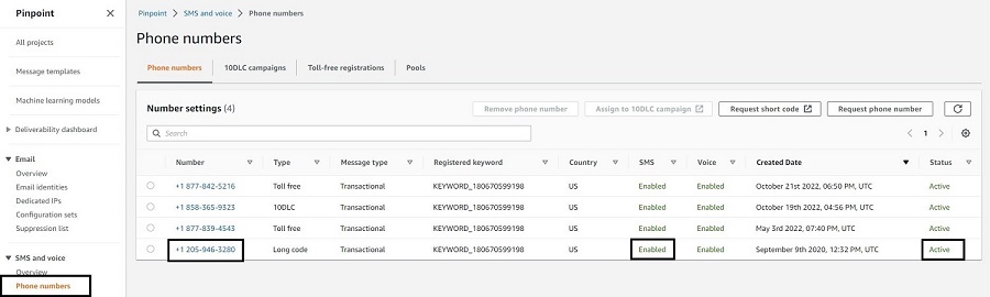
In Amazon Pinpoint > Phone numbers, Check to make sure the phone number you are using is enabled for SMS and its status is active.
Give a Bot name ‘Order Status’ under Bot name Configuration. (Use the same Bot name as mentioned here. If you change the Bot name here, your CloudFormation will fail)
Under IAM permissions, select the radio button Create a role with basic Amazon Lex permissions.
For COPPA, choose No. Click Next
Under Language dropdown, choose the language of usage. I chose Language as English in my example.
Click Done, to complete the Bot creation.
You have to create an Intent within the Bot you just created
Click on the Bot you just created. Click on Intents and click the dropdown Add intent and select Add empty intent.
Give an intent name and click Ok.
Once the intent is created, go to the intent and open the Conversation flow section in the intent and create a flow that that has the following info and looks like below image:
Click on Sample utterance and it takes you to Sample Utterance and type in Order status.
Click on initial response and type in Okay, I can help with that. What is your order number?
Click on the slot value and click on Add a slot. Name: OrderNumber and Slot type is AMAZON.AlphaNumeric. In the prompt, enter Please enter your order number.
Click on Save Intent button. The conversation flow should look like the below screenshot:
6. Go back to the Intent you just created and click on the Build button that is to the right side of the page.
7. Once the build is successfully completed, go back to the Bot you created and click on Aliases on the left frame. Click on the Alias that was created earlier, TestBotAlias.
8. In the Languages section, click on the English language that we created earlier. 9. Open the Lambda function – optional section and point the source to RE_Order_Validation Lambda that we downloaded earlier. 10. For Lambda function version or alias, select $LATEST. Click on Save.
11. Go to Intents, choose the intent you just built and click on Build button again. Once build is complete, you can test the intent.
Import and execute CloudFormation:
Navigate to the Amazon CloudFormation console in the AWS region you want to deploy this solution.
Select Create stack and With new resources. Choose Template is ready as Prerequisite – Prepare template and Upload a template file as Specify template. Upload the template downloaded in step 1 under Preparation section of this document. Click Next.
Fill the AWS CloudFormation parameters as shown below:
Stack name: Give a name to this stack.
Under Parameters, for BotAlias: The Bot Alias that you created as part of Amazon Lex above.
BotId: The Bot ID for the bot that you created as part of Amazon Lex above.
CodeS3Bucket: Give the name of the S3 bucket you created in step3 of the Preparation topic above.
OriginationNumber: This is the origination identity phone number you created in step4 of the Preparation topic above.
PinpointProjectId: Use the ProjectID you have from step2 of the Prerequisites phase above.
After entering all the parameter info, it would look something like this below:
Click Next. Leave the default options on the next page and click Next again.
Check the box I acknowledge that AWS CloudFormation might create IAM resources with custom names. Click Submit.
Set up data in Amazon Dynamo DB
We are using DynamoDB table here as the transactional database that stores order information for the bike store.
Once the solution has been successfully deployed, navigate to the Amazon DynamoDB console and access the OrderStatus DynamoDB table. Each row created in this table represents an order and it’s details. Each row should have a unique Order_Num that holds the order number and it’s related information. You can put additional information about the order like the example below:
Once you enter the data, it should look like the image below. Click on Create item.
Set up Amazon Simple Notification Service (SNS) topic
We need the Amazon Simple Notification Service here, to provide internal message delivery from publishers (customer’s text message) to subscribers (Amazon Lex in this example). This is used for internal notifications in this use case.
As part of the CloudFormation above, check if you have an SNS topic created by the name LexPinpointIntegrationDemo.
Now, we have successfully created an Amazon SNS topic.
Set up Lambda Functions
Go to AWS Lambda console and open the Lambda function LexIntegration. Under the Function overview, click on the Add trigger. Under Trigger configuration dropdown, select SNS and under SNS Topic select LexPinpointIntegrationDemo topic. Click on Add.
Note: In this example, I used Node.js in a Lambda and Python in another, to show how AWS Lambda functions are flexible to use the scripting language of your choice.
Setting up 2-way SMS in Amazon Pinpoint
Go to Amazon Pinpoint console and click on Phone numbers under SMS & Voice in the left frame. If you don’t see any phone numbers, please refer to #3 under prerequisites section above.
This is how your screen should look like
Click on the number.
On the right frame, expand Two-way SMS drop down arrow.
Click on the check box ‘Enable two-way SMS’.
In the ‘Incoming message destination’ select the radio button ‘Choose an existing SNS topic’ and in the drop down below, choose the SNS topic you built above.
The result would look like the screenshot below:
Click on Save.
Import Machine Learning model into Pinpoint
Go to Amazon Pinpoint.
Click on Machine Learning Models. Click on Add recommender model.
Give a recommender model name and description under model details.
Under Model configuration, choose the radio button ‘Automatically create a role’ and give an IAM role name in the textbox below.
Under recommender model, choose the recommender model campaign that you created in Amazon Personalize earlier in the project.
If you did not create it, use this Pinpoint workshop to create a recommender model in Amazon Personalize.
The data used in this example is for retail industry, please edit the data as needed for your use case and industry.
Under the settings section:
Select ‘User Id’ as identifier.
Click on the drop down ‘Number of recommendations per message’ and select 3.
For Processing method, choose ‘Use value returned by model’.
Click on Next.
You are presented with attributes section. Give a display name as ‘product_name’ for the attributes and click next.
On the next screen, you can review all the information provided and click on Publish.
The completed model after publishing looks like the screen below:
Once the template is created, you need to add recommendations to the message template using this Amazon Pinpoint Workshop details. Change the type of data needed for your use case and industry in this workshop. I used sample retail data.
To create a Amazon Pinpoint Journey, navigate to the Amazon Pinpoint console , select Journeys and click on Create journey.
Give a name, click on Set entry condition in the Journey entry block.
Choose the radio button Add participants when they perform an activity.
Click in the ‘Events’ text box and type in OrderStatus.
Click on Add activity and select Send an email.
Click on choose an email template and select the email message template we created earlier in this blog. Click on choose template button.
Select a Sender email address from the drop down list.
Click Save. The final journey should look like this:
Click on Actions > Settings where you will review the journey settings. There you set the start and end date of the journey if applicable as well as other advanced settings. Configure your journey settings to look like the screenshot below and click Save.
To publish your journey click on Review. On the Review your journey click Next > Mark as reviewed > Publish. A 5 minutes countdown will begin after, which your journey will be live.
Once the journey is live, we need to pass the event OrderStatus and the endpoints will go through that journey and will receive an email.
Testing the solution
Use a phone with a valid number (in this example, I took a US phone number) and send a text ‘Order Status’ to the number generated in Amazon Pinpoint above.
You should get a response “Okay, I can help with that. What is your order number?”
You should type in the order number you generated earlier and stored it in Amazon DynamoDB table.
You should get a response “Your order <order number> was shipped on <shipped_dt> and is expected to be delivered to your address on <delivery_dt>. Your order details have been emailed to you.”
Alternatively, you can test this solution from the Lex bot.
In Amazon Lex, go to the intent you created above and click on the Test button. Next steps:
In the text box, enter Order Status.
Bot should respond with Okay, I can help with that. What is your order number?
You can respond with the order number you entered in the DynamoDB table.
Bot should respond with Your order <Order_Num> was shipped on <Shipping_Dt> and is expected to be delivered to your address on <Delivery_Dt>. Your order details have been emailed to you.
Conclusion
Using this blog post, you can elevate your customer’s experience by using Amazon Lex’s AI chat capabilities, Amazon Personalize’s ML recommendation models and trigger a Pinpoint Journey. This blog highlights how organizations can interact in a 2-way SMS with their customers and convert that engagement to a triggered email, with product recommendations, if needed.
Next Steps
You can use the above solution and modify it easily to use it across different verticals and applicable use cases. You can also extend this solution to Amazon Connect to an agent via SMS chat, using this blog.
Clean-up
To delete the solution, go to CloudFormation you created as part od this project. Click on the stack and click Delete.
Navigate to Amazon Pinpoint and stop the Journey you ran in this solution. Delete the Journey, Machine learning models, Message templates you created for this solution. Delete the Project you created for this solution.
In Amazon Lex, delete the intent and bot you created for this solution.
Delete the folder and bucket you created in S3 as part of this project.
Amazon Personalize resources like Dataset groups, datasets, etc. are not created via AWS Cloudformation, thus you have to delete them manually. Please follow the instructions in the AWS documentation on how to clean up the created resources.
Vinay Ujjini is an Amazon Pinpoint and Amazon Simple Email Service Principal Specialist Solutions Architect at AWS. He has been solving customer’s omni-channel challenges for over 15 years. In his spare time, he enjoys playing tennis & cricket.
Each year, the research team at Rapid7 analyzes thousands of vulnerabilities in order to identify their root causes, broaden understanding of attacker behavior, and provide actionable intelligence that guides security professionals at critical moments. Our annual Vulnerability Intelligence Report examines notable vulnerabilities and high-impact attacks from 2022 to highlight trends that drive significant risk for organizations of all sizes.
Today, we’re excited to release Rapid7’s 2022 Vulnerability Intelligence Report—a deep dive into 50 of the most notable vulnerabilities our research team investigated throughout the year. The report offers insight into critical vulnerabilities, widespread threats, prominent attack surface area, and changing exploitation trends.
2022 attack trends
The threat landscape today is radically different than it was even a few years ago. Over the past three years, we’ve seen zero-day exploits and widespread attacks chart a meteoric rise that’s strained security teams to their breaking point and beyond. While 2022 saw a modest decline in zero-day and widespread exploitation from 2021’s record highs, the multi-year trend of rising attack speed and scale remains strikingly consistent overall.
Report findings include:
Widespread exploitation of newvulnerabilities decreased 15% year over year in 2022, but mass exploitation events were still the norm. Our 2022 vulnerability intelligence dataset tracks 28 net-new widespread threats, many of which were used to deploy webshells, cryptocurrency miners, botnet malware, and/or ransomware on target systems.
Zero-day exploitation remained a significant challenge for security teams, with 43% of widespread threats arising from a zero-day exploit.
Attackers are still developing and deploying exploits faster than ever before. More than half of the vulnerabilities in our report dataset were exploited within seven days of public disclosure—a 12% increase from 2021 and an 87% increase over 2020.
Vulnerabilities mapped definitively to ransomware operations dropped 33% year over year—a troubling trend that speaks more to evolving attacker behavior and lower industry visibility than to any actual reprieve for security practitioners. This year’s report explores the growing complexity of the cybercrime ecosystem, the rise of initial access brokers, and industry-wide ransomware reporting trends.
How to manage risk from critical vulnerabilities
In today’s threat landscape, security teams are frequently forced into reactive positions, lowering security program efficacy and sustainability. Strong foundational security program components, including vulnerability and asset management processes, are essential to building resilience in a persistently elevated threat climate.
Have emergency patching procedures and incident response playbooks in place so that in the event of a widespread threat or breach, your team has a well-understood mechanism to drive immediate action.
Have a defined, regular patch cycle that includes prioritization of actively exploited CVEs, as well as network edge technologies like VPNs and firewalls. These network edge devices continue to be popular attack vectors and should adhere to a zero-day patch cycle wherever possible, meaning that updates and/or downtime should be scheduled as soon as new critical advisories are released.
Keep up with operating system-level and cumulative updates. Falling behind on these regular updates can make it difficult to install out-of-band security patches at critical moments.
Limit and monitor internet exposure of critical infrastructure and services, including domain controllers and management or administrative interfaces. The exploitation of many of the CVEs in this year’s report could be slowed down or prevented by taking management interfaces off the public internet.
2022 Vulnerability Intelligence Report
Read the report to see our full list of high-priority CVEs and learn more about attack trends from 2022.
On April 1, 2018, Cloudflare announced the 1.1.1.1 public DNS resolver. Over the years, we added the debug page for troubleshooting, global cache purge, 0 TTL for zones on Cloudflare, Upstream TLS, and 1.1.1.1 for families to the platform. In this post, we would like to share some behind the scenes details and changes.
When the project started, Knot Resolver was chosen as the DNS resolver. We started building a whole system on top of it, so that it could fit Cloudflare’s use case. Having a battle tested DNS recursive resolver, as well as a DNSSEC validator, was fantastic because we could spend our energy elsewhere, instead of worrying about the DNS protocol implementation.
Knot Resolver is quite flexible in terms of its Lua-based plugin system. It allowed us to quickly extend the core functionality to support various product features, like DoH/DoT, logging, BPF-based attack mitigation, cache sharing, and iteration logic override. As the traffic grew, we reached certain limitations.
Lessons we learned
Before going any deeper, let’s first have a bird’s-eye view of a simplified Cloudflare data center setup, which could help us understand what we are going to talk about later. At Cloudflare, every server is identical: the software stack running on one server is exactly the same as on another server, only the configuration may be different. This setup greatly reduces the complexity of fleet maintenance.
Figure 1 Data center layout
The resolver runs as a daemon process, kresd, and it doesn’t work alone. Requests, specifically DNS requests, are load-balanced to the servers inside a data center by Unimog. DoH requests are terminated at our TLS terminator. Configs and other small pieces of data can be delivered worldwide by Quicksilver in seconds. With all the help, the resolver can concentrate on its own goal – resolving DNS queries, and not worrying about transport protocol details. Now let’s talk about 3 key areas we wanted to improve here – blocking I/O in plugins, a more efficient use of cache space, and plugin isolation.
Callbacks blocking the event loop
Knot Resolver has a very flexible plugin system for extending its core functionality. The plugins are called modules, and they are based on callbacks. At certain points during request processing, these callbacks will be invoked with current query context. This gives a module the ability to inspect, modify, and even produce requests / responses. By design, these callbacks are supposed to be simple, in order to avoid blocking the underlying event loop. This matters because the service is single threaded, and the event loop is in charge of serving many requests at the same time. So even just one request being held up in a callback means that no other concurrent requests can be progressed until the callback finishes.
The setup worked well enough for us until we needed to do blocking operations, for example, to pull data from Quicksilver before responding to the client.
Cache efficiency
As requests for a domain could land on any node inside a data center, it would be wasteful to repetitively resolve a query when another node already has the answer. By intuition, the latency could be improved if the cache could be shared among the servers, and so we created a cache module which multicasted the newly added cache entries. Nodes inside the same data center could then subscribe to the events and update their local cache.
The default cache implementation in Knot Resolver is LMDB. It is fast and reliable for small to medium deployments. But in our case, cache eviction shortly became a problem. The cache itself doesn’t track for any TTL, popularity, etc. When it’s full, it just clears all the entries and starts over. Scenarios like zone enumeration could fill the cache with data that is unlikely to be retrieved later.
Furthermore, our multicast cache module made it worse by amplifying the less useful data to all the nodes, and led them to the cache high watermark at the same time. Then we saw a latency spike because all the nodes dropped the cache and started over around the same time.
Module isolation
With the list of Lua modules increasing, debugging issues became increasingly difficult. This is because a single Lua state is shared among all the modules, so one misbehaving module could affect another. For example, when something went wrong inside the Lua state, like having too many coroutines, or being out of memory, we got lucky if the program just crashed, but the resulting stack traces were hard to read. It is also difficult to forcibly tear down, or upgrade, a running module as it not only has state in the Lua runtime, but also FFI, so memory safety is not guaranteed.
Hello BigPineapple
We didn’t find any existing software that would meet our somewhat niche requirements, so eventually we started building something ourselves. The first attempt was to wrap Knot Resolver’s core with a thin service written in Rust (modified edgedns).
This proved to be difficult due to having to constantly convert between the storage, and C/FFI types, and some other quirks (for example, the ABI for looking up records from cache expects the returned records to be immutable until the next call, or the end of the read transaction). But we learned a lot from trying to implement this sort of split functionality where the host (the service) provides some resources to the guest (resolver core library), and how we would make that interface better.
In the later iterations, we replaced the entire recursive library with a new one based around an async runtime; and a redesigned module system was added to it, sneakily rewriting the service into Rust over time as we swapped out more and more components. That async runtime was tokio, which offered a neat thread pool interface for running both non-blocking and blocking tasks, as well as a good ecosystem for working with other crates (Rust libraries).
After that, as the futures combinators became tedious, we started converting everything to async/await. This was before the async/await feature that landed in Rust 1.39, which led us to use nightly (Rust beta) for a while and had some hiccups. When the async/await stabilized, it enabled us to write our request processing routine ergonomically, similar to Go.
All the tasks can be run concurrently, and certain I/O heavy ones can be broken down into smaller pieces, to benefit from a more granular scheduling. As the runtime executes tasks on a threadpool, instead of a single thread, it also benefits from work stealing. This avoids a problem we previously had, where a single request taking a lot of time to process, that blocks all the other requests on the event loop.
Figure 2 Components overview
Finally, we forged a platform that we are happy with, and we call it BigPineapple. The figure above shows an overview of its main components and the data flow between them. Inside BigPineapple, the server module gets inbound requests from the client, validates and transforms them into unified frame streams, which can then be processed by the worker module. The worker module has a set of workers, whose task is to figure out the answer to the question in the request. Each worker interacts with the cache module to check if the answer is there and still valid, otherwise it drives the recursor module to recursively iterate the query. The recursor doesn’t do any I/O, when it needs anything, it delegates the sub-task to the conductor module. The conductor then uses outbound queries to get the information from upstream nameservers. Through the whole process, some modules can interact with the Sandbox module, to extend its functionality by running the plugins inside.
Let’s look at some of them in more detail, and see how they helped us overcome the problems we had before.
Updated I/O architecture
A DNS resolver can be seen as an agent between a client and several authoritative nameservers: it receives requests from the client, recursively fetches data from the upstream nameservers, then composes the responses and sends them back to the client. So it has both inbound and outbound traffic, which are handled by the server and the conductor component respectively.
The server listens on a list of interfaces using different transport protocols. These are later abstracted into streams of “frames”. Each frame is a high level representation of a DNS message, with some extra metadata. Underneath, it can be a UDP packet, a segment of TCP stream, or the payload of a HTTP request, but they are all processed the same way. The frame is then converted into an asynchronous task, which in turn is picked up by a set of workers in charge of resolving these tasks. The finished tasks are converted back into responses, and sent back to the client.
This “frame” abstraction over the protocols and their encodings simplified the logic used to regulate the frame sources, such as enforcing fairness to prevent starving and controlling pacing to protect the server from being overwhelmed. One of the things we’ve learned with the previous implementations is that, for a service open to the public, a peak performance of the I/O matters less than the ability to pace clients fairly. This is mainly because the time and computational cost of each recursive request is vastly different (for example a cache hit from a cache miss), and it’s difficult to guess it beforehand. The cache misses in recursive service not only consume Cloudflare’s resources, but also the resources of the authoritative nameservers being queried, so we need to be mindful of that.
On the other side of the server is the conductor, which manages all the outbound connections. It helps to answer some questions before reaching out to the upstream: Which is the fastest nameserver to connect to in terms of latency? What to do if all the nameservers are not reachable? What protocol to use for the connection, and are there any better options? The conductor is able to make these decisions by tracking the upstream server’s metrics, such as RTT, QoS, etc. With that knowledge, it can also guess for things like upstream capacity, UDP packet loss, and take necessary actions, e.g. retry when it thinks the previous UDP packet didn’t reach the upstream.
Figure 3 I/O conductor
Figure 3 shows a simplified data flow about the conductor. It is called by the exchanger mentioned above, with upstream requests as input. The requests will be deduplicated first: meaning in a small window, if a lot of requests come to the conductor and ask for the same question, only one of them will pass, the others are put into a waiting queue. This is common when a cache entry expires, and can reduce unnecessary network traffic. Then based on the request and upstream metrics, the connection instructor either picks an open connection if available, or generates a set of parameters. With these parameters, the I/O executor is able to connect to the upstream directly, or even take a route via another Cloudflare data center using our Argo Smart Routing technology!
The cache
Caching in a recursive service is critical as a server can return a cached response in under one millisecond, while it will be hundreds of milliseconds to respond on a cache miss. As the memory is a finite resource (and also a shared resource in Cloudflare’s architecture), more efficient use of space for cache was one of the key areas we wanted to improve. The new cache is implemented with a cache replacement data structure (ARC), instead of a KV store. This makes good use of the space on a single node, as less popular entries are progressively evicted, and the data structure is resistant to scans.
Moreover, instead of duplicating the cache across the whole data center with multicast, as we did before, BigPineapple is aware of its peer nodes in the same data center, and relays queries from one node to another if it cannot find an entry in its own cache. This is done by consistent hashing the queries onto the healthy nodes in each data center. So, for example, queries for the same registered domain go through the same subset of nodes, which not only increases the cache hit ratio, but also helps the infrastructure cache, which stores information about performance and features of nameservers.
Figure 4 Updated data center layout
Async recursive library
The recursive library is the DNS brain of BigPineapple, as it knows how to find the answer to the question in the query. Starting from the root, it breaks down the client query into subqueries, and uses them to collect knowledge recursively from various authoritative nameservers on the internet. The product of this process is the answer. Thanks to the async/await it can be abstracted as a function like such:
The function contains all the logic necessary to generate a response to a given request, but it doesn’t do any I/O on its own. Instead, we pass an Exchanger trait(Rust interface) that knows how to exchange DNS messages with upstream authoritative nameservers asynchronously. The exchanger is usually called at various await points – for example, when a recursion starts, one of the first things it does is that it looks up the closest cached delegation for the domain. If it doesn’t have the final delegation in cache, it needs to ask what nameservers are responsible for this domain and wait for the response, before it can proceed any further.
Thanks to this design, which decouples the “waiting for some responses” part from the recursive DNS logic, it is much easier to test by providing a mock implementation of the exchanger. In addition, it makes the recursive iteration code (and DNSSEC validation logic in particular) much more readable, as it’s written sequentially instead of being scattered across many callbacks.
Fun fact: writing a DNS recursive resolver from scratch is not fun at all!
Not only because of the complexity of DNSSEC validation, but also because of the necessary “workarounds” needed for various RFC incompatible servers, forwarders, firewalls, etc. So we ported deckard into Rust to help test it. Additionally, when we started migrating over to this new async recursive library, we first ran it in “shadow” mode: processing real world query samples from the production service, and comparing differences. We’ve done this in the past on Cloudflare’s authoritative DNS service as well. It is slightly more difficult for a recursive service due to the fact that a recursive service has to look up all the data over the Internet, and authoritative nameservers often give different answers for the same query due to localization, load balancing and such, leading to many false positives.
In December 2019, we finally enabled the new service on a public test endpoint (see the announcement) to iron out remaining issues before slowly migrating the production endpoints to the new service. Even after all that, we continued to find edge cases with the DNS recursion (and DNSSEC validation in particular), but fixing and reproducing these issues has become much easier due to the new architecture of the library.
Sandboxed plugins
Having the ability to extend the core DNS functionality on the fly is important for us, thus BigPineapple has its redesigned plugin system. Before, the Lua plugins run in the same memory space as the service itself, and are generally free to do what they want. This is convenient, as we can freely pass memory references between the service and modules using C/FFI. For example, to read a response directly from cache without having to copy to a buffer first. But it is also dangerous, as the module can read uninitialized memory, call a host ABI using a wrong function signature, block on a local socket, or do other undesirable things, in addition the service doesn’t have a way to restrict these behaviors.
So we looked at replacing the embedded Lua runtime with JavaScript, or native modules, but around the same time, embedded runtimes for WebAssembly (Wasm for short) started to appear. Two nice properties of WebAssembly programs are that it allows us to write them in the same language as the rest of the service, and that they run in an isolated memory space. So we started modeling the guest/host interface around the limitations of WebAssembly modules, to see how that would work.
BigPineapple’s Wasm runtime is currently powered by Wasmer. We tried several runtimes over time like Wasmtime, WAVM in the beginning, and found Wasmer was simpler to use in our case. The runtime allows each module to run in its own instance, with an isolated memory and a signal trap, which naturally solved the module isolation problem we described before. In addition to this, we can have multiple instances of the same module running at the same time. Being controlled carefully, the apps can be hot swapped from one instance to another without missing a single request! This is great because the apps can be upgraded on the fly without a server restart. Given that the Wasm programs are distributed via Quicksilver, BigPineapple’s functionality can be safely changed worldwide within a few seconds!
To better understand the WebAssembly sandbox, several terms need to be introduced first:
Host: the program which runs the Wasm runtime. Similar to a kernel, it has full control through the runtime over the guest applications.
Guest application: the Wasm program inside the sandbox. Within a restricted environment, it can only access its own memory space, which is provided by the runtime, and call the imported Host calls. We call it an app for short.
Host call: the functions defined in the host that can be imported by the guest. Comparable to syscall, it’s the only way guest apps can access the resources outside the sandbox.
Guest runtime: a library for guest applications to easily interact with the host. It implements some common interfaces, so an app can just use async, socket, log and tracing without knowing the underlying details.
Now it’s time to dive into the sandbox, so stay awhile and listen. First let’s start from the guest side, and see what a common app lifespan looks like. With the help of the guest runtime, guest apps can be written similar to regular programs. So like other executables, an app begins with a start function as an entrypoint, which is called by the host upon loading. It is also provided with arguments as from the command line. At this point, the instance normally does some initialization, and more importantly, registers callback functions for different query phases. This is because in a recursive resolver, a query has to go through several phases before it gathers enough information to produce a response, for example a cache lookup, or making subrequests to resolve a delegation chain for the domain, so being able to tie into these phases is necessary for the apps to be useful for different use cases. The start function can also run some background tasks to supplement the phase callbacks, and store global state. For example – report metrics, or pre-fetch shared data from external sources, etc. Again, just like how we write a normal program.
But where do the program arguments come from? How could a guest app send log and metrics? The answer is, external functions.
Figure 5 Wasm based Sandbox
In figure 5, we can see a barrier in the middle, which is the sandbox boundary, that separates the guest from the host. The only way one side can reach out to the other, is via a set of functions exported by the peer beforehand. As in the picture, the “hostcalls” are exported by the host, imported and called by the guest; while the “trampoline” are guest functions that the host has knowledge of.
It is called trampoline because it is used to invoke a function or a closure inside a guest instance that’s not exported. The phase callbacks are one example of why we need a trampoline function: each callback returns a closure, and therefore can’t be exported on instantiation. So a guest app wants to register a callback, it calls a host call with the callback address “hostcall_register_callback(pre_cache, #30987)”, when the callback needs to be invoked, the host cannot just call that pointer as it’s pointing to the guest’s memory space. What it can do instead is, to leverage one of the aforementioned trampolines, and give it the address of the callback closure: “trampoline_call(#30987)”.
Isolation overhead Like a coin that has two sides, the new sandbox does come with some additional overhead. The portability and isolation that WebAssembly offers bring extra cost. Here, we’ll list two examples.
Firstly, guest apps are not allowed to read host memory. The way it works is the guest provides a memory region via a host call, then the host writes the data into the guest memory space. This introduces a memory copy that would not be needed if we were outside the sandbox. The bad news is, in our use case, the guest apps are supposed to do something on the query and/or the response, so they almost always need to read data from the host on every single request. The good news, on the other hand, is that during a request life cycle, the data won’t change. So we pre-allocate a bulk of memory in the guest memory space right after the guest app instantiates. The allocated memory is not going to be used, but instead serves to occupy a hole in the address space. Once the host gets the address details, it maps a shared memory region with the common data needed by the guest into the guest’s space. When the guest code starts to execute, it can just access the data in the shared memory overlay, and no copy is needed.
Another issue we ran into was when we wanted to add support for a modern protocol, oDoH, into BigPineapple. The main job of it is to decrypt the client query, resolve it, then encrypt the answers before sending it back. By design, this doesn’t belong to core DNS, and should instead be extended with a Wasm app. However, the WebAssembly instruction set doesn’t provide some crypto primitives, such as AES and SHA-2, which prevents it from getting the benefit of host hardware. There is ongoing work to bring this functionality to Wasm with WASI-crypto. Until then, our solution for this is to simply delegate the HPKE to the host via host calls, and we already saw 4x performance improvements, compared to doing it inside Wasm.
Async in Wasm Remember the problem we talked about before that the callbacks could block the event loop? Essentially, the problem is how to run the sandboxed code asynchronously. Because no matter how complex the request processing callback is, if it can yield, we can put an upper bound on how long it is allowed to block. Luckily, Rust’s async framework is both elegant and lightweight. It gives us the opportunity to use a set of guest calls to implement the “Future”s.
In Rust, a Future is a building block for asynchronous computations. From the user’s perspective, in order to make an asynchronous program, one has to take care of two things: implement a pollable function that drives the state transition, and place a waker as a callback to wake itself up, when the pollable function should be called again due to some external event (e.g. time passes, socket becomes readable, and so on). The former is to be able to progress the program gradually, e.g. read buffered data from I/O and return a new state indicating the status of the task: either finished, or yielded. The latter is useful in case of task yielding, as it will trigger the Future to be polled when the conditions that the task was waiting for are fulfilled, instead of busy looping until it’s complete.
Let’s see how this is implemented in our sandbox. For a scenario when the guest needs to do some I/O, it has to do so via the host calls, as it is inside a restricted environment. Assuming the host provides a set of simplified host calls which mirror the basic socket operations: open, read, write, and close, the guest can have its pseudo poller defined as below:
Here the host call reads data from a socket into a buffer, depending on its return value, the function can move itself to one of the states we mentioned above: finished(Ready), or yielded(Pending). The magic happens inside the host call. Remember in figure 5, that it is the only way to access resources? The guest app doesn’t own the socket, but it can acquire a “handle” via “hostcall_socket_open”, which will in turn create a socket on the host side, and return a handle. The handle can be anything in theory, but in practice using integer socket handles map well to file descriptors on the host side, or indices in a vector or slab. By referencing the returned handle, the guest app is able to remotely control the real socket. As the host side is fully asynchronous, it can simply relay the socket state to the guest. If you noticed that the waker function isn’t used above, well done! That’s because when the host call is called, it not only starts opening a socket, but also registers the current waker to be called then the socket is opened (or fails to do so). So when the socket becomes ready, the host task will be woken up, it will find the corresponding guest task from its context, and wakes it up using the trampoline function as shown in figure 5. There are other cases where a guest task needs to wait for another guest task, an async mutex for example. The mechanism here is similar: using host calls to register wakers.
All of these complicated things are encapsulated in our guest async runtime, with easy to use API, so the guest apps get access to regular async functions without having to worry about the underlying details.
(Not) The End
Hopefully, this blog post gave you a general idea of the innovative platform that powers 1.1.1.1. It is still evolving. As of today, several of our products, such as 1.1.1.1 for Families, AS112, and Gateway DNS, are supported by guest apps running on BigPineapple. We are looking forward to bringing new technologies into it. If you have any ideas, please let us know in the community or via email.
To provide the best experiences, we use technologies like cookies to store and/or access device information. Consenting to these technologies will allow us to process data such as browsing behavior or unique IDs on this site. Not consenting or withdrawing consent, may adversely affect certain features and functions.
Functional
Always active
The technical storage or access is strictly necessary for the legitimate purpose of enabling the use of a specific service explicitly requested by the subscriber or user, or for the sole purpose of carrying out the transmission of a communication over an electronic communications network.
Preferences
The technical storage or access is necessary for the legitimate purpose of storing preferences that are not requested by the subscriber or user.
Statistics
The technical storage or access that is used exclusively for statistical purposes.The technical storage or access that is used exclusively for anonymous statistical purposes. Without a subpoena, voluntary compliance on the part of your Internet Service Provider, or additional records from a third party, information stored or retrieved for this purpose alone cannot usually be used to identify you.
Marketing
The technical storage or access is required to create user profiles to send advertising, or to track the user on a website or across several websites for similar marketing purposes.
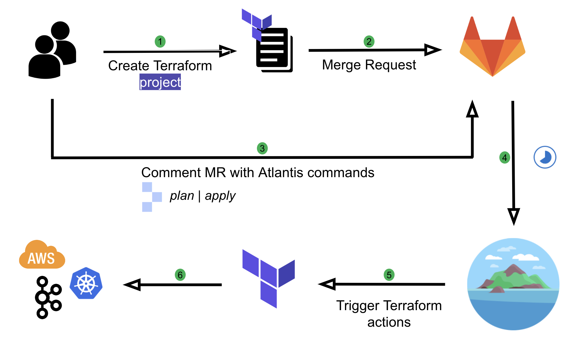
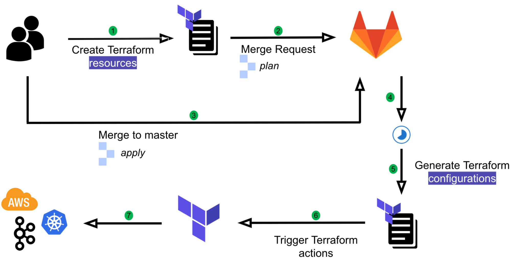
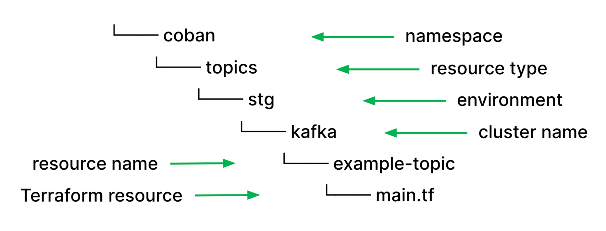
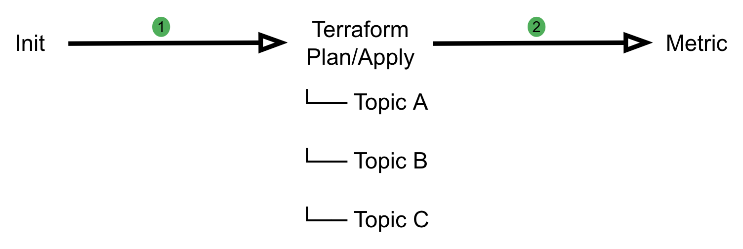
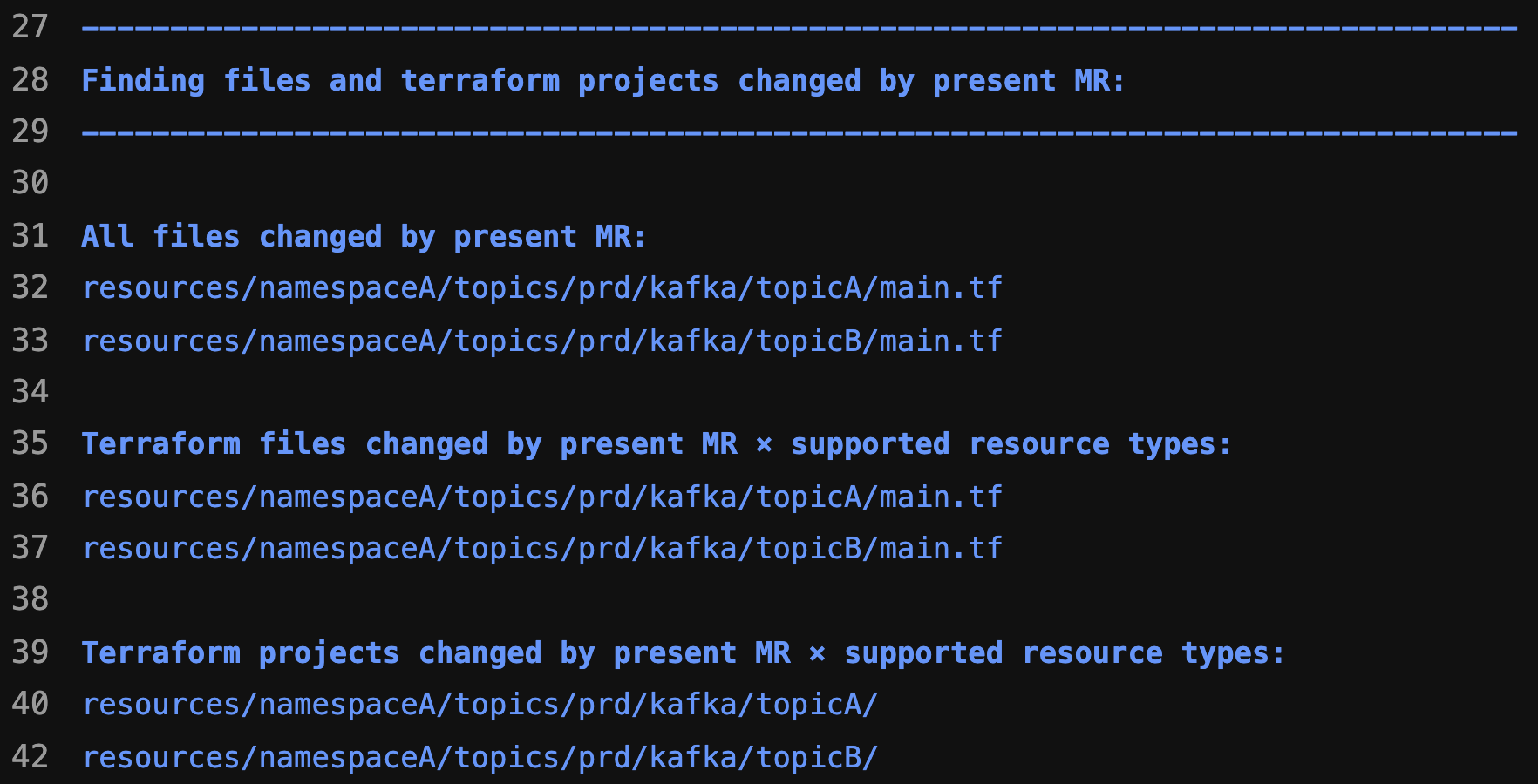
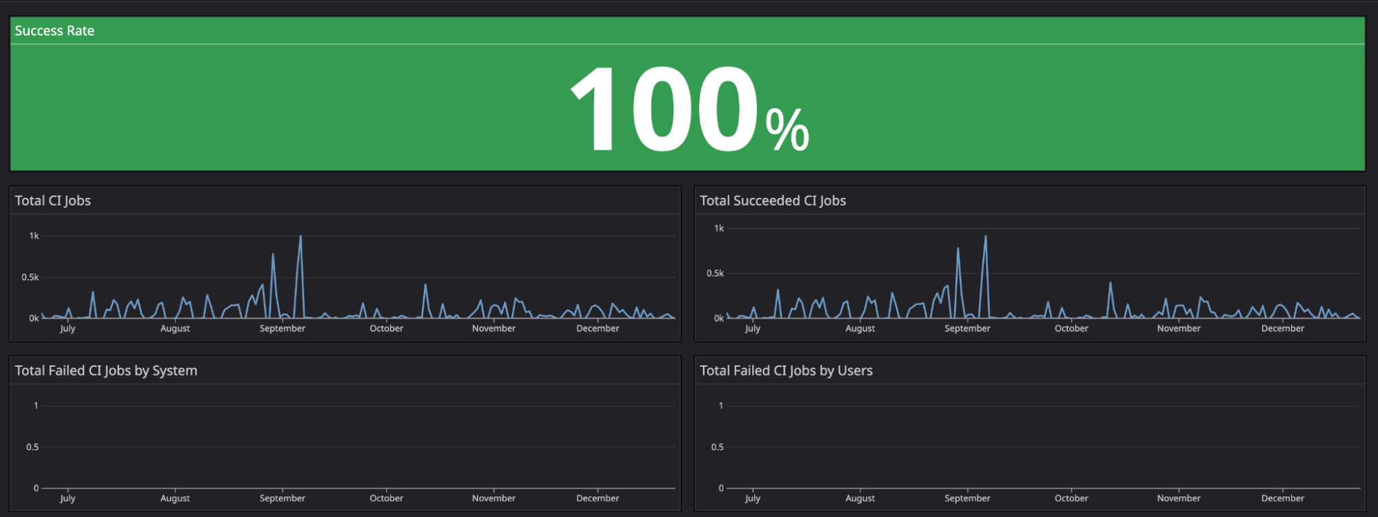

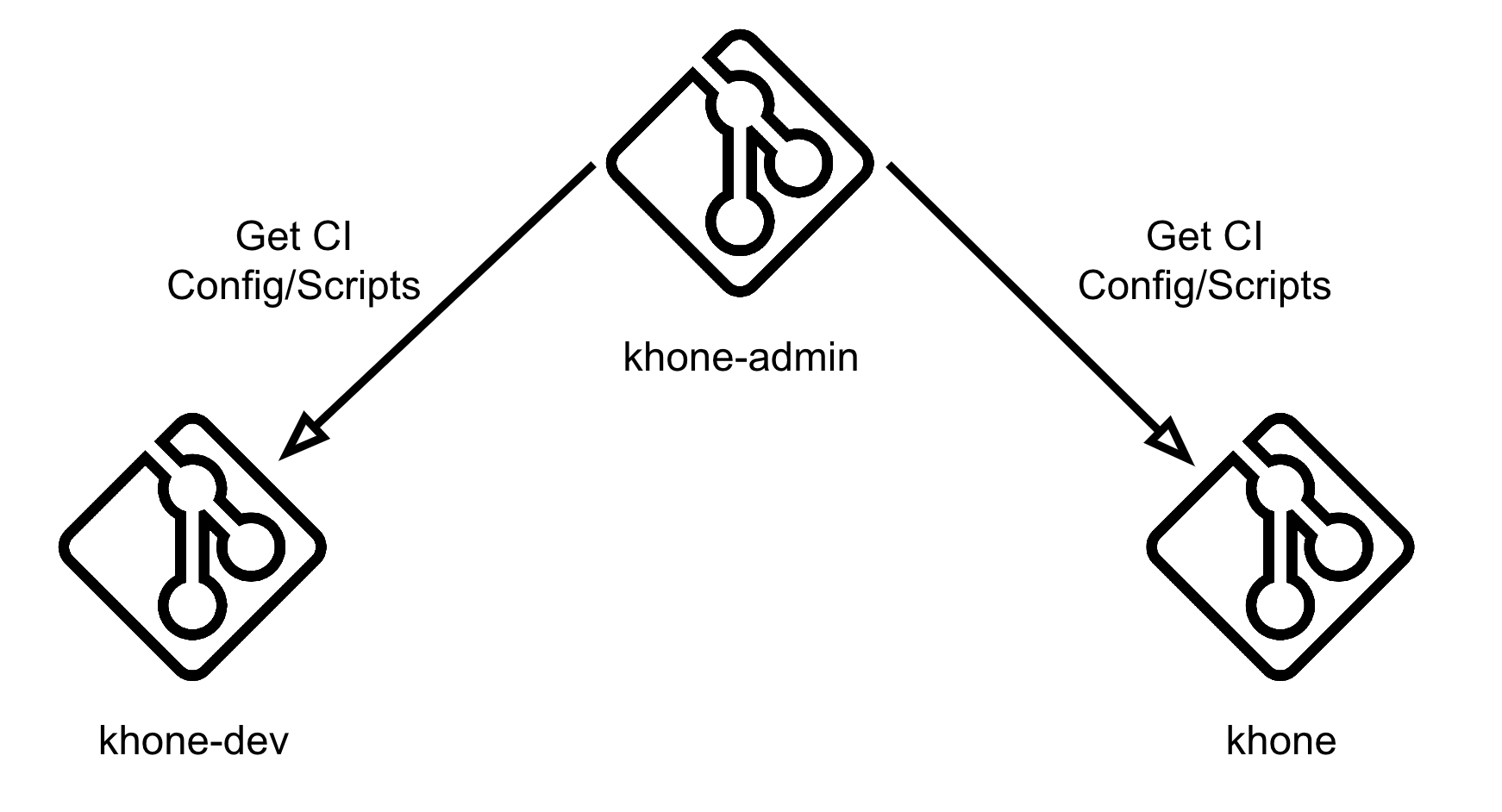

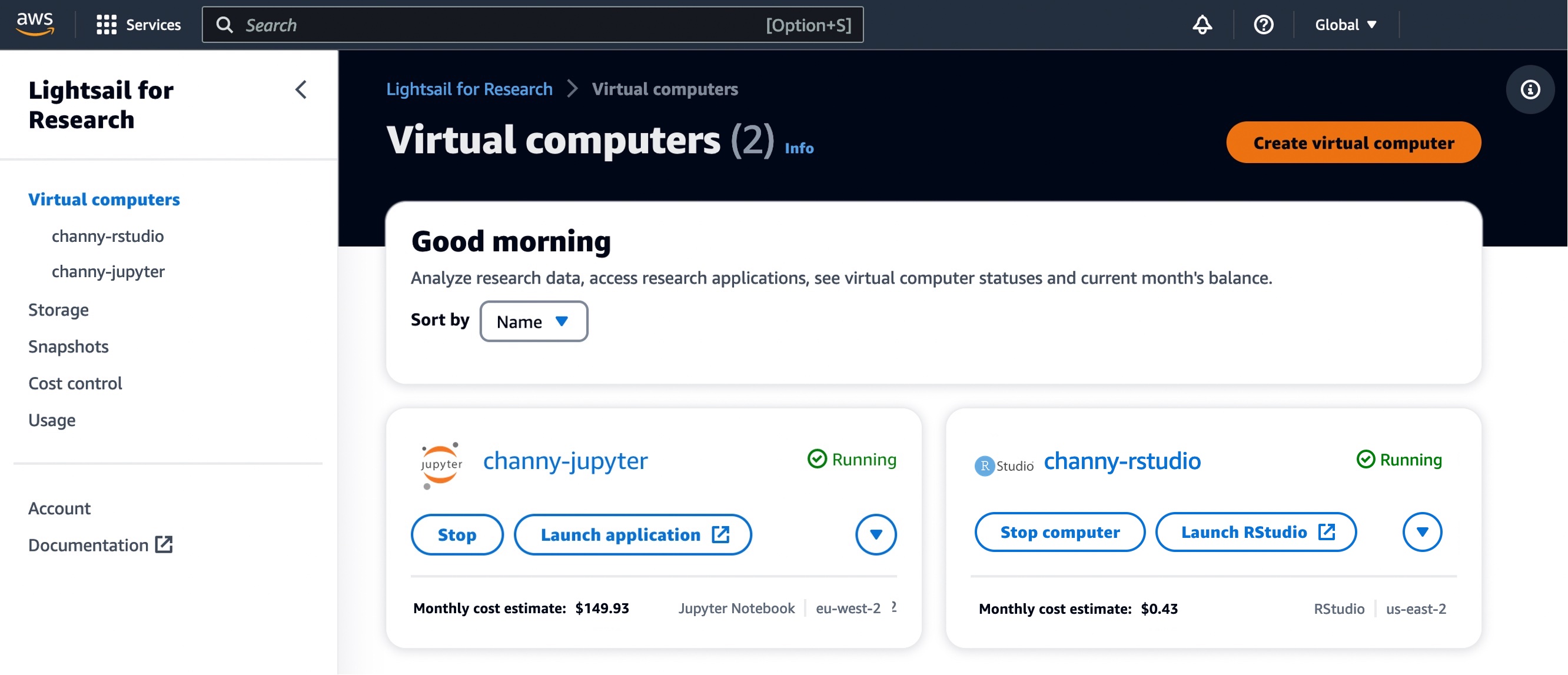

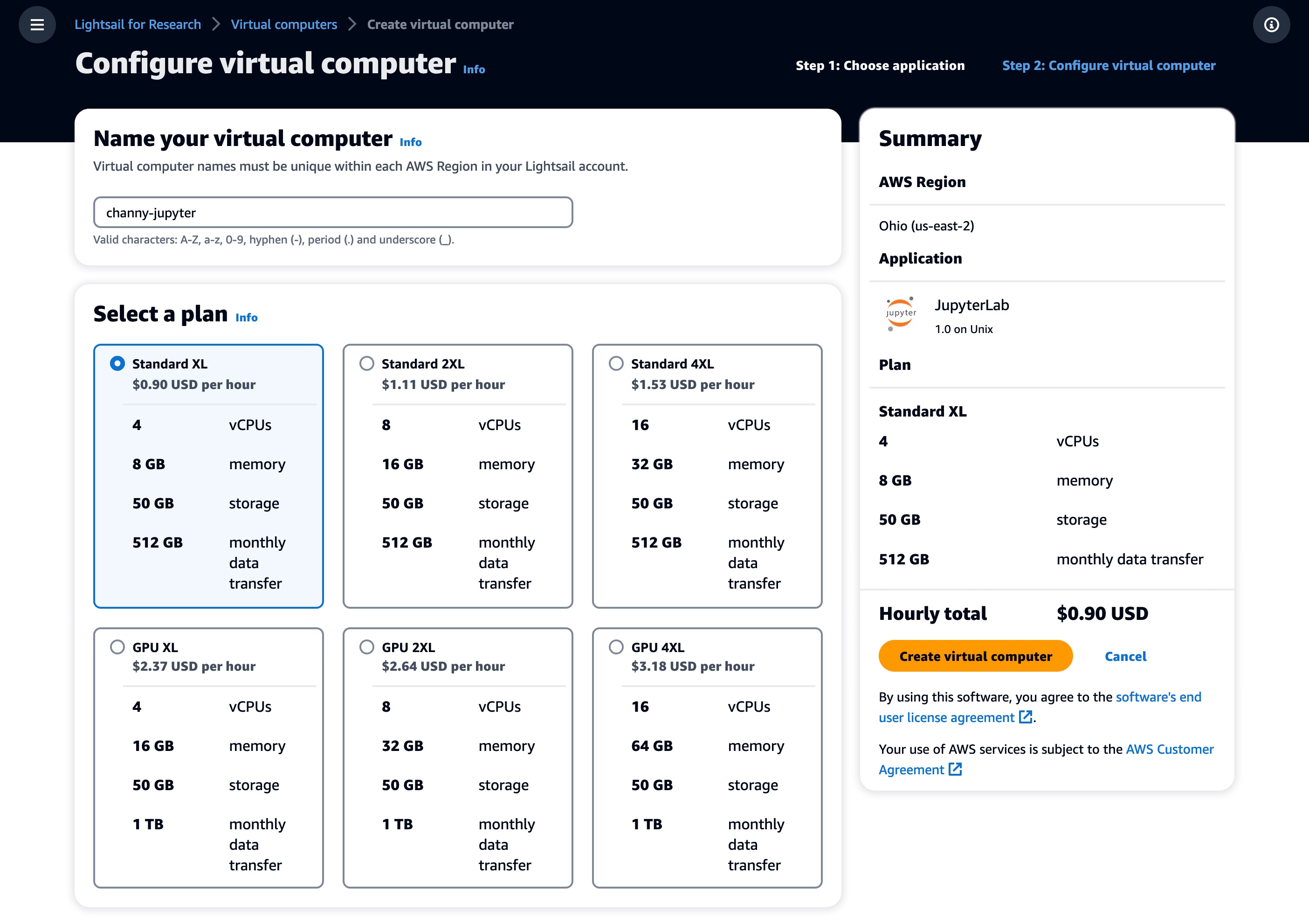
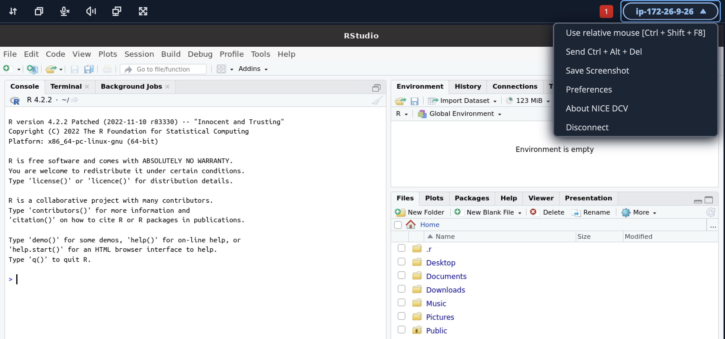
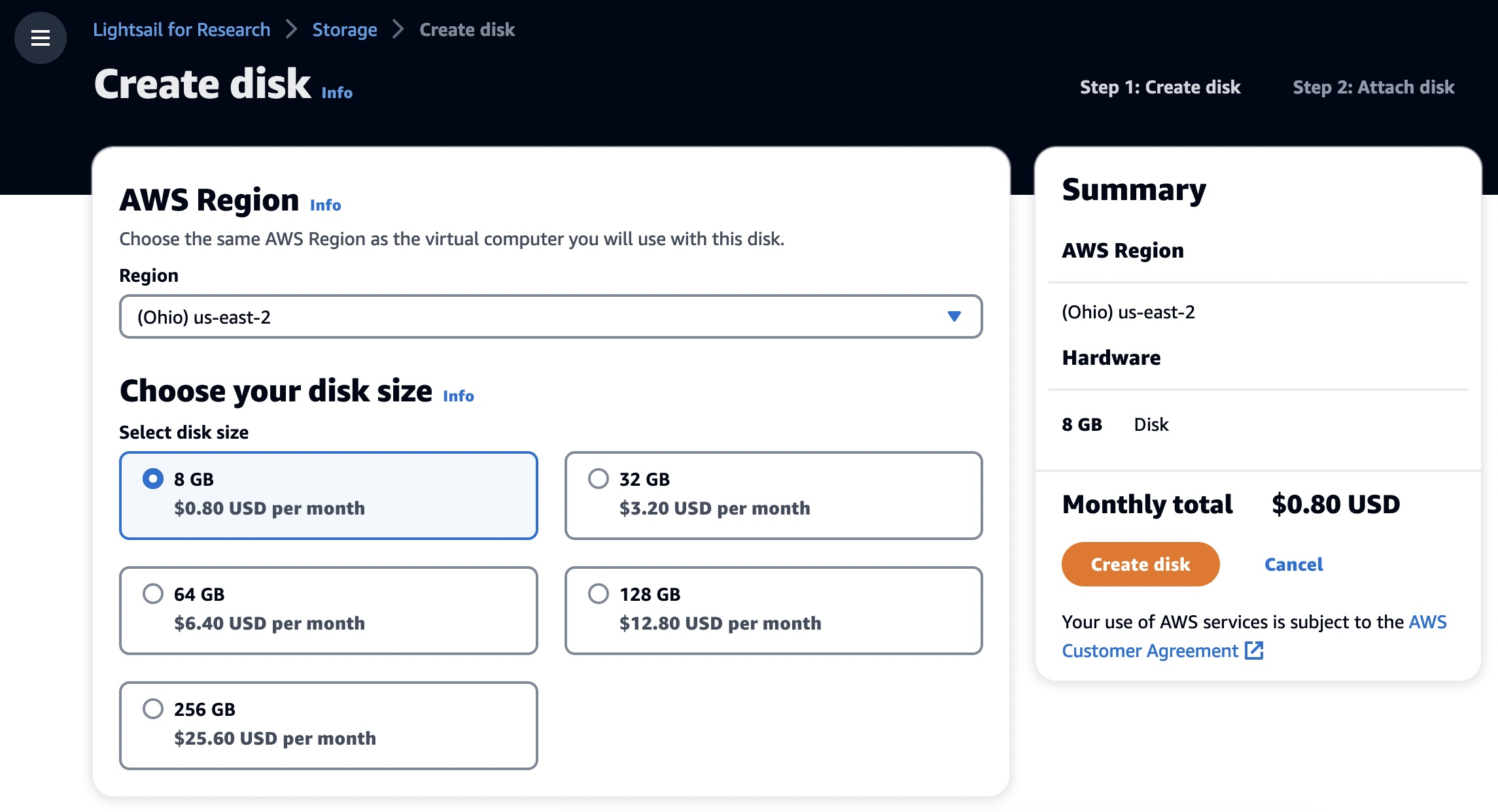
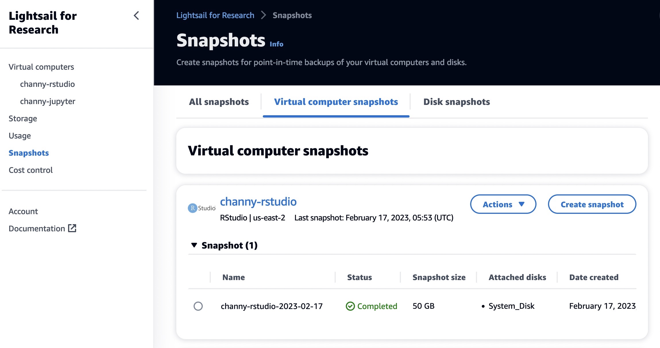
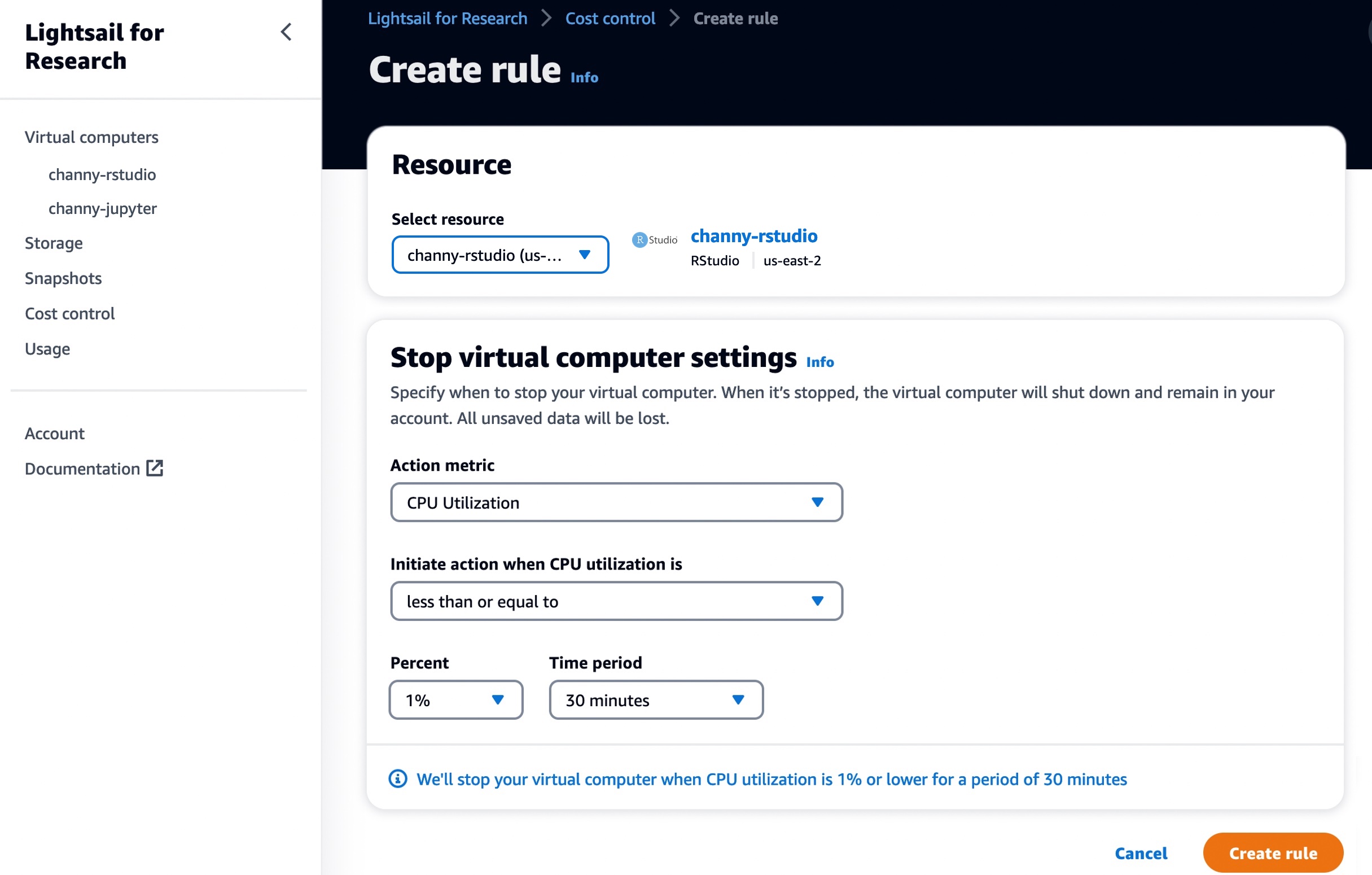
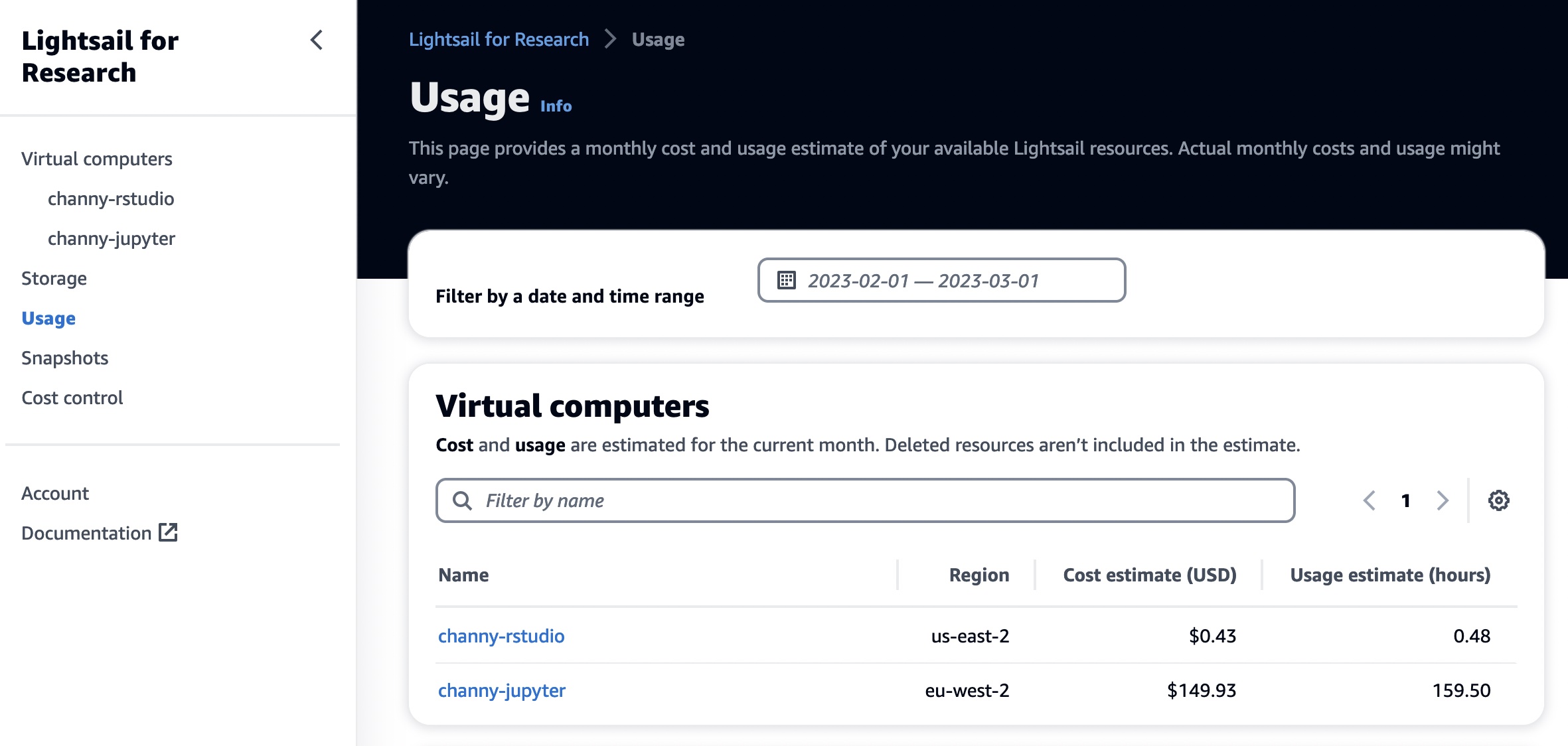



 Sushant Majithia is a Principal Product Manager for EMR at Amazon Web Services.
 Vishal Vyas is a Senior Software Engineer for EMR at Amazon Web Services.
 Matthew Liem is a Senior Solution Architecture Manager at AWS.




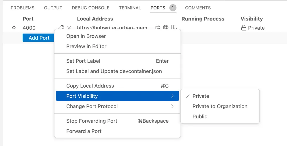
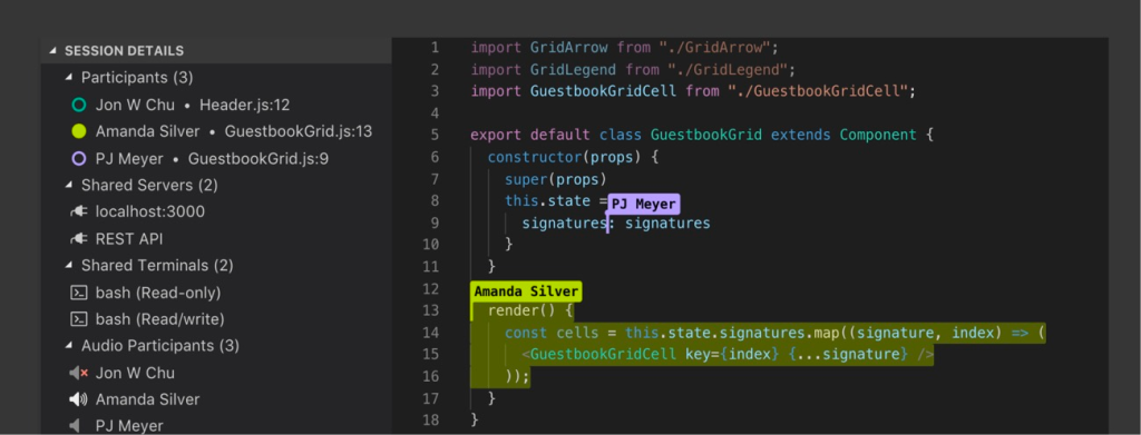

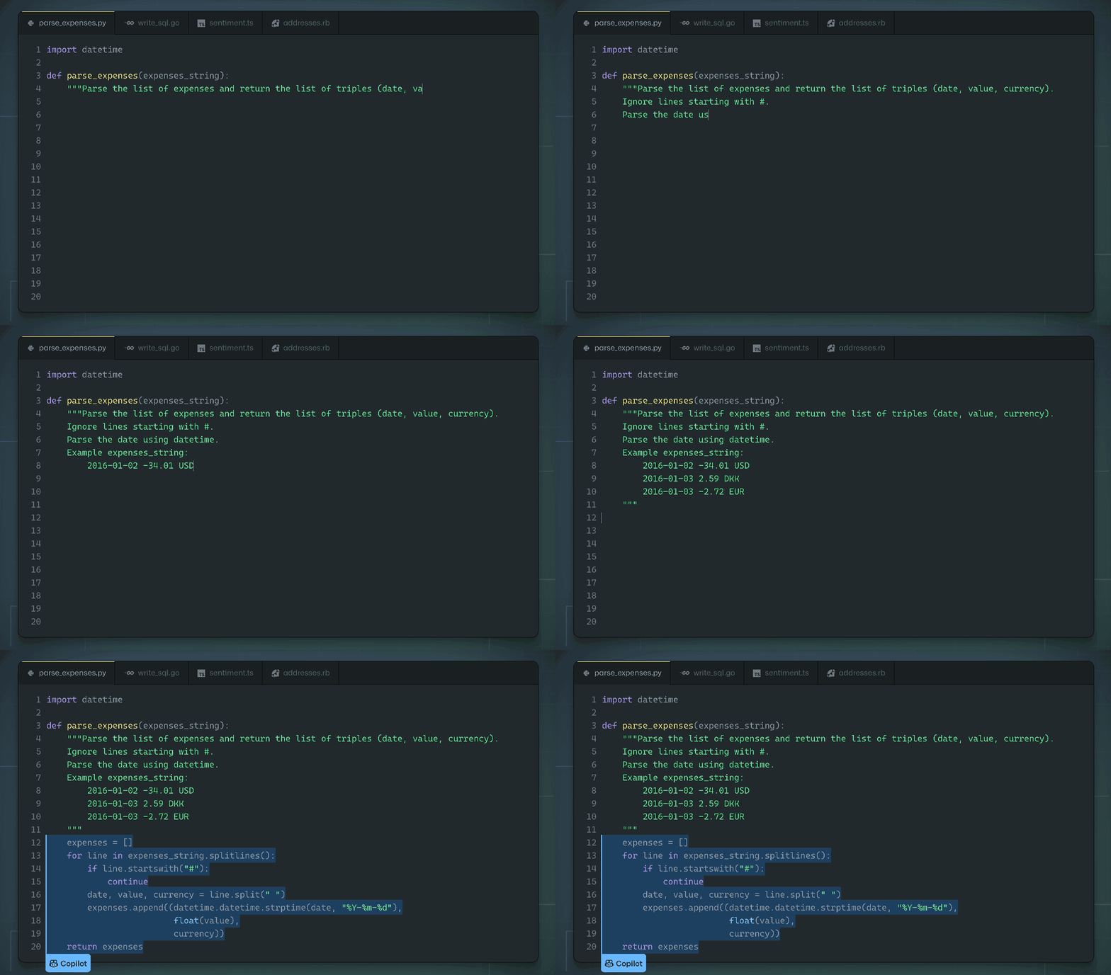


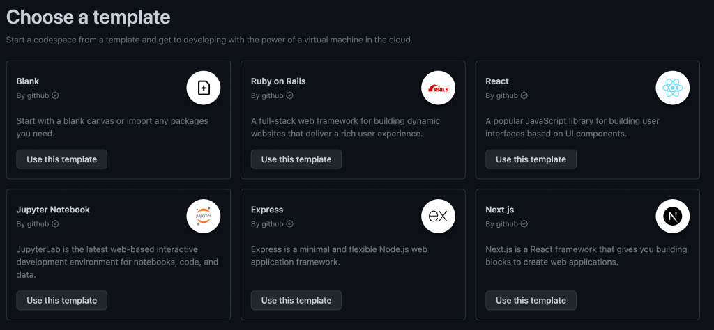

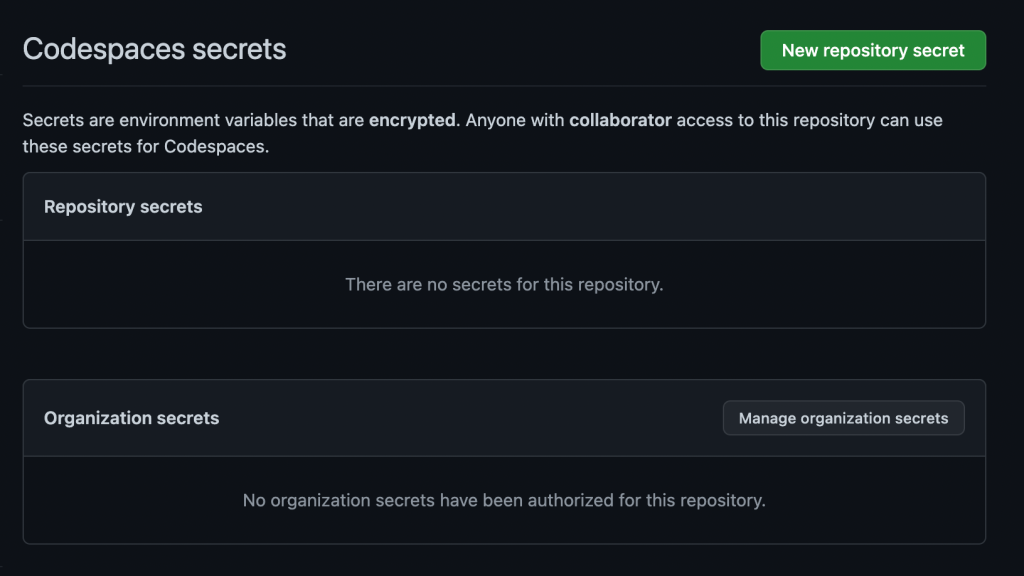





 Satesh Sonti is a Sr. Analytics Specialist Solutions Architect based out of Atlanta, specialized in building enterprise data platforms, data warehousing, and analytics solutions. He has over 16 years of experience in building data assets and leading complex data platform programs for banking and insurance clients across the globe.
 Yanzhu Ji is a Product Manager on the Amazon Redshift team. She worked on the Amazon Redshift team as a Software Engineer before becoming a Product Manager. She has a rich experience of how the customer-facing Amazon Redshift features are built from planning to launching, and always treats customers’ requirements as first priority. In her personal life, Yanzhu likes painting, photography, and playing tennis.
 Dinesh Kumar is a Database Engineer with more than a decade of experience working in the databases, data warehousing, and analytics space. Outside of work, he enjoys trying different cuisines and spending time with his family and friends.