Post Syndicated from Bartlomiej Plotka (@bwplotka) original https://prometheus.io/blog/2021/11/16/agent/
Bartek Płotka has been a Prometheus Maintainer since 2019 and Principal Software Engineer at Red Hat. Co-author of the CNCF Thanos project. CNCF Ambassador and tech lead for the CNCF TAG Observability. In his free time, he writes a book titled “Efficient Go” with O’Reilly. Opinions are my own!
What I personally love in the Prometheus project, and one of the many reasons why I joined the team, was the laser focus on the project’s goals. Prometheus was always about pushing boundaries when it comes to providing pragmatic, reliable, cheap, yet invaluable metric-based monitoring. Prometheus’ ultra-stable and robust APIs, query language, and integration protocols (e.g. Remote Write and OpenMetrics) allowed the Cloud Native Computing Foundation (CNCF) metrics ecosystem to grow on those strong foundations. Amazing things happened as a result:
- We can see community exporters for getting metrics about virtually everything e.g. containers, eBPF, Minecraft server statistics and even plants’ health when gardening.
- Most people nowadays expect cloud-native software to have an HTTP/HTTPS
/metrics endpoint that Prometheus can scrape. A concept developed in secret within Google and pioneered globally by the Prometheus project.
- The observability paradigm shifted. We see SREs and developers rely heavily on metrics from day one, which improves software resiliency, debuggability, and data-driven decisions!
In the end, we hardly see Kubernetes clusters without Prometheus running there.
The strong focus of the Prometheus community allowed other open-source projects to grow too to extend the Prometheus deployment model beyond single nodes (e.g. Cortex, Thanos and more). Not mentioning cloud vendors adopting Prometheus’ API and data model (e.g. Amazon Managed Prometheus, Google Cloud Managed Prometheus, Grafana Cloud and more). If you are looking for a single reason why the Prometheus project is so successful, it is this: Focusing the monitoring community on what matters.
In this (lengthy) blog post, I would love to introduce a new operational mode of running Prometheus called “Agent”. It is built directly into the Prometheus binary. The agent mode disables some of Prometheus’ usual features and optimizes the binary for scraping and remote writing to remote locations. Introducing a mode that reduces the number of features enables new usage patters. In this blog post I will explain why it is a game-changer for certain deployments in the CNCF ecosystem. I am super excited about this!
History of the Forwarding Use Case
The core design of Prometheus has been unchanged for the project’s entire lifetime. Inspired by Google’s Borgmon monitoring system, you can deploy a Prometheus server alongside the applications you want to monitor, tell Prometheus how to reach them, and allow to scrape the current values of their metrics at regular intervals. Such a collection method, which is often referred to as the “pull model”, is the core principle that allows Prometheus to be lightweight and reliable. Furthermore, it enables application instrumentation and exporters to be dead simple, as they only need to provide a simple human-readable HTTP endpoint with the current value of all tracked metrics (in OpenMetrics format). All without complex push infrastructure and non-trivial client libraries. Overall, a simplified typical Prometheus monitoring deployment looks as below:

This works great, and we have seen millions of successful deployments like this over the years that process dozens of millions of active series. Some of them for longer time retention, like two years or so. All allow to query, alert, and record metrics useful for both cluster admins and developers.
However, the cloud-native world is constantly growing and evolving. With the growth of managed Kubernetes solutions and clusters created on-demand within seconds, we are now finally able to treat clusters as “cattle”, not as “pets” (in other words, we care less about individual instances of those). In some cases, solutions do not even have the cluster notion anymore, e.g. kcp, Fargate and other platforms.
The other interesting use case that emerges is the notion of Edge clusters or networks. With industries like telecommunication, automotive and IoT devices adopting cloud-native technologies, we see more and more much smaller clusters with a restricted amount of resources. This is forcing all data (including observability) to be transferred to remote, bigger counterparts as almost nothing can be stored on those remote nodes.
What does that mean? That means monitoring data has to be somehow aggregated, presented to users and sometimes even stored on the global level. This is often called a Global-View feature.
Naively, we could think about implementing this by either putting Prometheus on that global level and scraping metrics across remote networks or pushing metrics directly from the application to the central location for monitoring purposes. Let me explain why both are generally very bad ideas:
🔥 Scraping across network boundaries can be a challenge if it adds new unknowns in a monitoring pipeline. The local pull model allows Prometheus to know why exactly the metric target has problems and when. Maybe it’s down, misconfigured, restarted, too slow to give us metrics (e.g. CPU saturated), not discoverable by service discovery, we don’t have credentials to access or just DNS, network, or the whole cluster is down. By putting our scraper outside of the network, we risk losing some of this information by introducing unreliability into scrapes that is unrelated to an individual target. On top of that, we risk losing important visibility completely if the network is temporarily down. Please don’t do it. It’s not worth it. (:
🔥 Pushing metrics directly from the application to some central location is equally bad. Especially when you monitor a larger fleet, you know literally nothing when you don’t see metrics from remote applications. Is the application down? Is my receiver pipeline down? Maybe the application failed to authorize? Maybe it failed to get the IP address of my remote cluster? Maybe it’s too slow? Maybe the network is down? Worse, you may not even know that the data from some application targets is missing. And you don’t even gain a lot as you need to track the state and status of everything that should be sending data. Such a design needs careful analysis as it can be a recipe for a failure too easily.
NOTE: Serverless functions and short-living containers are often cases where we think about push from application as the rescue. At this point however we talk about events or pieces of metrics we might want to aggregate to longer living time series. This topic is discussed
here, feel free to contribute and help us support those cases better!
Prometheus introduced three ways to support the global view case, each with its own pros and cons. Let’s briefly go through those. They are shown in orange color in the diagram below:
-
Federation was introduced as the first feature for aggregation purposes. It allows a global-level Prometheus server to scrape a subset of metrics from a leaf Prometheus. Such a “federation” scrape reduces some unknowns across networks because metrics exposed by federation endpoints include the original samples’ timestamps. Yet, it usually suffers from the inability to federate all metrics and not lose data during longer network partitions (minutes).
-
Prometheus Remote Read allows selecting raw metrics from a remote Prometheus server’s database without a direct PromQL query. You can deploy Prometheus or other solutions (e.g. Thanos) on the global level to perform PromQL queries on this data while fetching the required metrics from multiple remote locations. This is really powerful as it allows you to store data “locally” and access it only when needed. Unfortunately, there are cons too. Without features like Query Pushdown we are in extreme cases pulling GBs of compressed metric data to answer a single query. Also, if we have a network partition, we are temporarily blind. Last but not least, certain security guidelines are not allowing ingress traffic, only egress one.
- Finally, we have Prometheus Remote Write, which seems to be the most popular choice nowadays. Since the agent mode focuses on remote write use cases, let’s explain it in more detail.
Remote Write
The Prometheus Remote Write protocol allows us to forward (stream) all or a subset of metrics collected by Prometheus to the remote location. You can configure Prometheus to forward some metrics (if you want, with all metadata and exemplars!) to one or more locations that support the Remote Write API. In fact, Prometheus supports both ingesting and sending Remote Write, so you can deploy Prometheus on a global level to receive that stream and aggregate data cross-cluster.
While the official Prometheus Remote Write API specification is in review stage, the ecosystem adopted the Remote Write protocol as the default metrics export protocol. For example, Cortex, Thanos, OpenTelemetry, and cloud services like Amazon, Google, Grafana, Logz.io, etc., all support ingesting data via Remote Write.
The Prometheus project also offers the official compliance tests for its APIs, e.g. remote-write sender compliance for solutions that offer Remote Write client capabilities. It’s an amazing way to quickly tell if you are correctly implementing this protocol.
Streaming data from such a scraper enables Global View use cases by allowing you to store metrics data in a centralized location. This also enables separation of concerns, which is useful when applications are managed by different teams than the observability or monitoring pipelines. Furthermore, it is also why Remote Write is chosen by vendors who want to offload as much work from their customers as possible.
Wait for a second, Bartek. You just mentioned before that pushing metrics directly from the application is not the best idea!
Sure, but the amazing part is that, even with Remote Write, Prometheus still uses a pull model to gather metrics from applications, which gives us an understanding of those different failure modes. After that, we batch samples and series and export, replicate (push) data to the Remote Write endpoints, limiting the number of monitoring unknowns that the central point has!
It’s important to note that a reliable and efficient remote-writing implementation is a non-trivial problem to solve. The Prometheus community spent around three years to come up with a stable and scalable implementation. We reimplemented the WAL (write-ahead-log) a few times, added internal queuing, sharding, smart back-offs and more. All of this is hidden from the user, who can enjoy well-performing streaming or large amounts of metrics stored in a centralized location.
Hands-on Remote Write Example: Katacoda Tutorial
All of this is not new in Prometheus. Many of us already use Prometheus to scrape all required metrics and remote-write all or some of them to remote locations.
Suppose you would like to try the hands-on experience of remote writing capabilities. In that case, we recommend the Thanos Katacoda tutorial of remote writing metrics from Prometheus, which explains all steps required for Prometheus to forward all metrics to the remote location. It’s free, just sign up for an account and enjoy the tutorial! 🤗
Note that this example uses Thanos in receive mode as the remote storage. Nowadays, you can use plenty of other projects that are compatible with the remote write API.
So if remote writing works fine, why did we add a special Agent mode to Prometheus?
Prometheus Agent Mode
From Prometheus v2.32.0 (next release), everyone will be able to run the Prometheus binary with an experimental --enable-feature=agent flag. If you want to try it before the release, feel free to use Prometheus v2.32.0-beta.0 or use our quay.io/prometheus/prometheus:v2.32.0-beta.0 image.
The Agent mode optimizes Prometheus for the remote write use case. It disables querying, alerting, and local storage, and replaces it with a customized TSDB WAL. Everything else stays the same: scraping logic, service discovery and related configuration. It can be used as a drop-in replacement for Prometheus if you want to just forward your data to a remote Prometheus server or any other Remote-Write-compliant project. In essence it looks like this:
The best part about Prometheus Agent is that it’s built into Prometheus. Same scraping APIs, same semantics, same configuration and discovery mechanism.
What are the benefits of using the Agent mode if you plan not to query or alert on data locally and stream metrics outside? There are a few:
First of all, efficiency. Our customized Agent TSDB WAL removes the data immediately after successful writes. If it cannot reach the remote endpoint, it persists the data temporarily on the disk until the remote endpoint is back online. This is currently limited to a two-hour buffer only, similar to non-agent Prometheus, hopefully unblocked soon. This means that we don’t need to build chunks of data in memory. We don’t need to maintain a full index for querying purposes. Essentially the Agent mode uses a fraction of the resources that a normal Prometheus server would use in a similar situation.
Does this efficiency matter? Yes! As we mentioned, every GB of memory and every CPU core used on edge clusters matters for some deployments. On the other hand, the paradigm of performing monitoring using metrics is quite mature these days. This means that the more relevant metrics with more cardinality you can ship for the same cost – the better.
NOTE: With the introduction of the Agent mode, the original Prometheus server mode still stays as the recommended, stable and maintained mode. Agent mode with remote storage brings additional complexity. Use with care.
Secondly, the benefit of the new Agent mode is that it enables easier horizontal scalability for ingestion. This is something I am excited about the most. Let me explain why.
The Dream: Auto-Scalable Metric Ingestion
A true auto-scalable solution for scraping would need to be based on the amount of metric targets and the number of metrics they expose. The more data we have to scrape, the more instances of Prometheus we deploy automatically. If the number of targets or their number of metrics goes down, we could scale down and remove a couple of instances. This would remove the manual burden of adjusting the sizing of Prometheus and stop the need for over-allocating Prometheus for situations where the cluster is temporarily small.
With just Prometheus in server mode, this was hard to achieve. This is because Prometheus in server mode is stateful. Whatever is collected stays as-is in a single place. This means that the scale-down procedure would need to back up the collected data to existing instances before termination. Then we would have the problem of overlapping scrapes, misleading staleness markers etc.
On top of that, we would need some global view query that is able to aggregate all samples across all instances (e.g. Thanos Query or Promxy). Last but not least, the resource usage of Prometheus in server mode depends on more things than just ingestion. There is alerting, recording, querying, compaction, remote write etc., that might need more or fewer resources independent of the number of metric targets.
Agent mode essentially moves the discovery, scraping and remote writing to a separate microservice. This allows a focused operational model on ingestion only. As a result, Prometheus in Agent mode is more or less stateless. Yes, to avoid loss of metrics, we need to deploy an HA pair of agents and attach a persistent disk to them. But technically speaking, if we have thousands of metric targets (e.g. containers), we can deploy multiple Prometheus agents and safely change which replica is scraping which targets. This is because, in the end, all samples will be pushed to the same central storage.
Overall, Prometheus in Agent mode enables easy horizontal auto-scaling capabilities of Prometheus-based scraping that can react to dynamic changes in metric targets. This is definitely something we will look at with the Prometheus Kubernetes Operator community going forward.
Now let’s take a look at the currently implemented state of agent mode in Prometheus. Is it ready to use?
Agent Mode Was Proven at Scale
The next release of Prometheus will include Agent mode as an experimental feature. Flags, APIs and WAL format on disk might change. But the performance of the implementation is already battle-tested thanks to Grafana Labs’ open-source work.
The initial implementation of our Agent’s custom WAL was inspired by the current Prometheus server’s TSDB WAL and created by Robert Fratto in 2019, under the mentorship of Tom Wilkie, Prometheus maintainer. It was then used in an open-source Grafana Agent project that was since then used by many Grafana Cloud customers and community members. Given the maturity of the solution, it was time to donate the implementation to Prometheus for native integration and bigger adoption. Robert (Grafana Labs), with the help of Srikrishna (Red Hat) and the community, ported the code to the Prometheus codebase, which was merged to main 2 weeks ago!
The donation process was quite smooth. Since some Prometheus maintainers contributed to this code before within the Grafana Agent, and since the new WAL is inspired by Prometheus’ own WAL, it was not hard for the current Prometheus TSDB maintainers to take it under full maintenance! It also really helps that Robert is joining the Prometheus Team as a TSDB maintainer (congratulations!).
Now, let’s explain how you can use it! (:
How to Use Agent Mode in Detail
From now on, if you show the help output of Prometheus (--help flag), you should see more or less the following:
usage: prometheus [<flags>]

The Prometheus monitoring server

Flags:
  -h, --help                     Show context-sensitive help (also try --help-long and --help-man).
      (... other flags)
      --storage.tsdb.path="data/"
                                 Base path for metrics storage. Use with server mode only.
      --storage.agent.path="data-agent/"
                                 Base path for metrics storage. Use with agent mode only.
      (... other flags)
      --enable-feature= ...      Comma separated feature names to enable. Valid options: agent, exemplar-storage, expand-external-labels, memory-snapshot-on-shutdown, promql-at-modifier, promql-negative-offset, remote-write-receiver,
                                 extra-scrape-metrics, new-service-discovery-manager. See https://prometheus.io/docs/prometheus/latest/feature_flags/ for more details.
Since the Agent mode is behind a feature flag, as mentioned previously, use the --enable-feature=agent flag to run Prometheus in the Agent mode. Now, the rest of the flags are either for both server and Agent or only for a specific mode. You can see which flag is for which mode by checking the last sentence of a flag’s help string. “Use with server mode only” means it’s only for server mode. If you don’t see any mention like this, it means the flag is shared.
The Agent mode accepts the same scrape configuration with the same discovery options and remote write options.
It also exposes a web UI with disabled query capabitilies, but showing build info, configuration, targets and service discovery information as in a normal Prometheus server.
Hands-on Prometheus Agent Example: Katacoda Tutorial
Similarly to Prometheus remote-write tutorial, if you would like to try the hands-on experience of Prometheus Agent capabilities, we recommend the Thanos Katacoda tutorial of Prometheus Agent, which explains how easy it is to run Prometheus Agent.
Summary
I hope you found this interesting! In this post, we walked through the new cases that emerged like:
- edge clusters
- limited access networks
- large number of clusters
- ephemeral and dynamic clusters
We then explained the new Prometheus Agent mode that allows efficiently forwarding scraped metrics to the remote write endpoints.
As always, if you have any issues or feedback, feel free to submit a ticket on GitHub or ask questions on the mailing list.
This blog post is part of a coordinated release between CNCF, Grafana, and Prometheus. Feel free to also read the CNCF announcement and the angle on the Grafana Agent which underlies the Prometheus Agent.


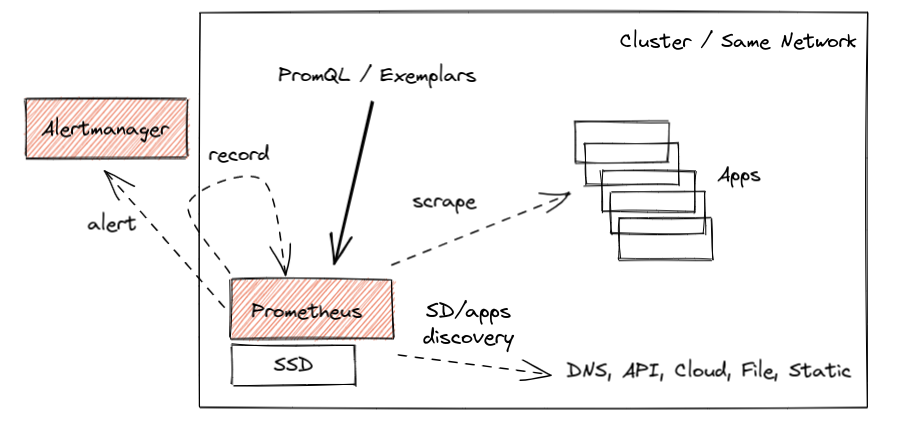

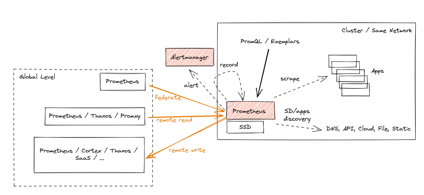
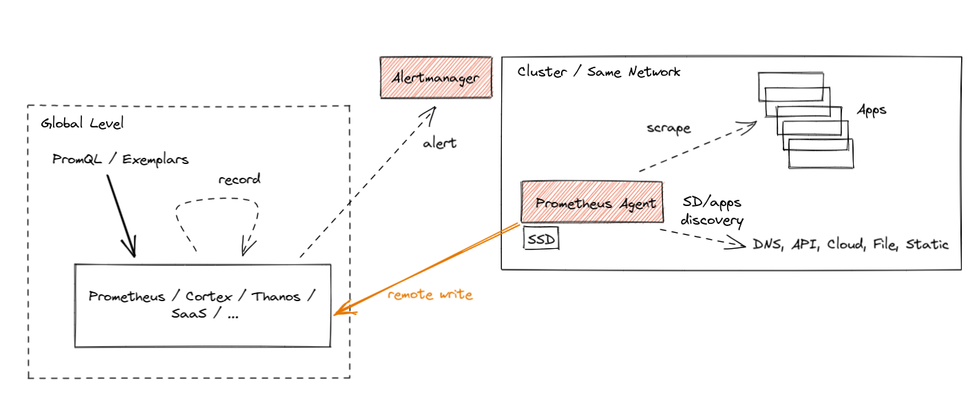


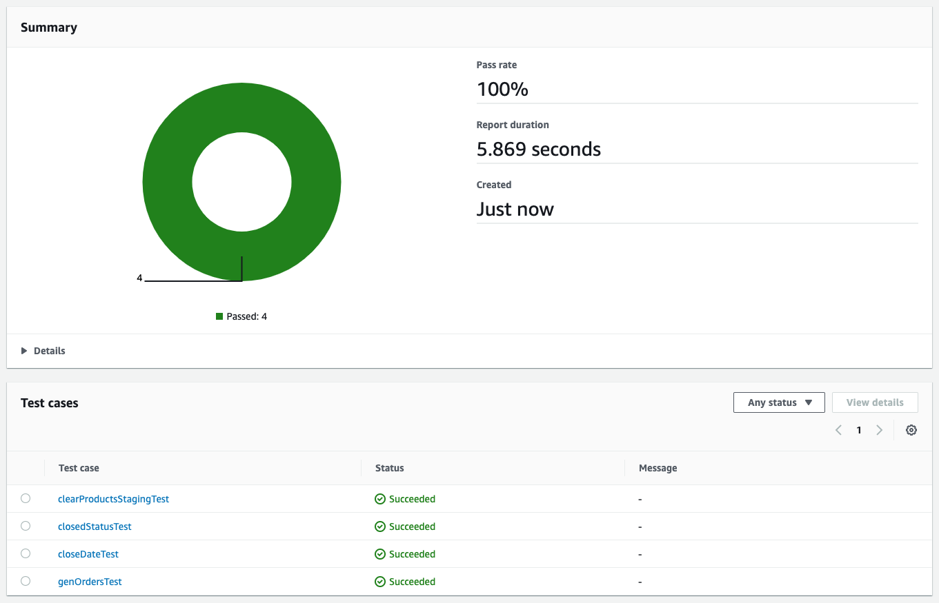


 Figure 1. AVA displays anomalies raised from L4E. A prediction score of > 0 indicates that an anomaly has been detected, and AVA will raise an issue with the underlying sensor details.