Build a high-performance, ACID compliant, evolving data lake using Apache Iceberg on Amazon EMR

Post Syndicated from Sekar Srinivasan original https://aws.amazon.com/blogs/big-data/build-a-high-performance-acid-compliant-evolving-data-lake-using-apache-iceberg-on-amazon-emr/

Amazon EMR is a cloud big data platform for running large-scale distributed data processing jobs, interactive SQL queries, and machine learning (ML) applications using open-source analytics frameworks such as Apache Spark, Apache Hive, and Presto.

Apache Iceberg is an open table format for huge analytic datasets. Table formats typically indicate the format and location of individual table files. Iceberg adds functionality on top of that to help manage petabyte-scale datasets as well as newer data lake requirements such as transactions, upsert/merge, time travel, and schema and partition evolution. Iceberg adds tables to compute engines including Spark, Trino, PrestoDB, Flink, and Hive using a high-performance table format that works just like a SQL table.

Amazon EMR release 6.5.0 and later includes Apache Iceberg so you can reliably work with huge tables with full support for ACID (Atomic, Consistent, Isolated, Durable) transactions in a highly concurrent and performant manner without getting locked into a single file format.

In this post, we discuss the modern data lake requirements and the challenges—including support for ACID transactions and concurrent writers, partition and schema evolution—that come with these. We also discuss how Iceberg solves these challenges. Additionally, we provide a step-by-step guide on how to get started with an Iceberg notebook in Amazon EMR Studio. You can access this sample notebook from the GitHub repo. You can also find this notebook in your EMR Studio workspace under Notebook Examples.

Modern data lake challenges

Amazon EMR integrates with Amazon Simple Storage Service (Amazon S3) natively for persistent data storage, and allows you to independently scale your data in Amazon S3 and compute on your EMR cluster. This enables you to bring in data from multiple sources (for example, transactional data from operational databases, social media feeds, and SaaS data sources) using different tools, and each data source has its own transient EMR cluster to perform transformation and ingestion in parallel. You can now keep one central copy of your data and share it with multiple user groups that run analytics and even make in-place updates on a data lake. We’re increasingly seeing the following requirements (and challenges) emerge as mainstream:

  • Consistent reads and writes across multiple concurrent users – There are two primary concerns:
    • Reader-writer isolation – When a job is updating a huge dataset, another job accessing the same data frequently works on a partially updated dataset, leaving the data in an inconsistent state.
    • Concurrent writes on the same dataset – Table formats relying on coarse-grained locks slow down the system. This limitation is even more telling in real-time streaming workloads.
  • Consistent table updates across multiple files or partitions – With Hive tables, writing to multiple partitions at once isn’t an atomic operation. If you’re overwriting a partition, for instance, you might delete several files across partitions without having any guarantees that you will replace them, potentially resulting in data loss. For huge tables, it’s not practical to use global locks and keep the readers and writers waiting. Common workarounds (such as rewriting all the data in all the partitions that need to be changed at the same time and then pointing to the new locations) cause huge data duplication and redundant extract, transform, and load (ETL) jobs.
  • Continuous schema evolution – Simple DDL commands often render the data unusable. For instance, say a data engineer renames a column and writes some data. The consuming analytics tool now can’t read it because the metastore can’t track former names for columns. That rename operation has effectively dropped a column and added a new column. Now there is data written in both schemas. Historically, schema changes required expensive backfills and redundant ETL processes.
  • Different query patterns on the same data – If you change the partitioning to optimize your query after a year, say from daily to hourly, you have to rewrite the table with the new hour column as the partition. In addition, you have to rewrite queries to use the new partition column in your table.
  • ACID transactions, streaming upserts, file size optimization, and data snapshots – Existing tools that support these features lock you into specific file formats, complicating interoperability across the analytics ecosystem.
  • Support for mixed file formats – With existing solutions, if you rename a column in one file format (say Parquet, ORC, or Avro), you get a different behavior than if you rename a column in a different file format. There is inconsistency in data types supported by different file formats. These limitations necessitate additional ETL steps.

The problem

When multiple users share the same data, varied requirements ensue. The data platform needs to be transactional to handle concurrent upserts and reads.

Table formats such as Hive track a list of partitions inside the table within a data catalog. However, the underlying files are still not tracked transactionally, because we’re relying on an immutable object storage that is just not designed to be transactional. After the specific partitions to be updated or inserted have been identified, we still need to list all the files in those partitions at the leaf level of the partition hierarchy before we can filter out which of those files are relevant. For huge analytic datasets with thousands of files in each partition, listing all those files each time you run a query slows it down considerably. Furthermore, doing atomic commits—getting thousands of files in the table live in exactly the same moment—becomes impractical.

Apache Iceberg on Amazon EMR

Iceberg development was started by Netflix in December 2017 and was donated to the Apache software foundation in November 2018 as an incubator project. In May 2020, it graduated from the incubator.

Iceberg on Amazon EMR comes completely integrated and tested for running in production backed by Enterprise Support. This means you get 24/7 technical support from Amazon EMR experts, tools and technology to automatically manage the health of your environment, and consultative architectural, performance, and troubleshooting guidance on Iceberg issues.

Iceberg has integrations with other AWS services. For example, you can use the AWS Glue Data Catalog as the metastore for Iceberg tables. Iceberg also supports other catalog types such as Hive, Hadoop, Amazon DynamoDB, Amazon Relational Database Service (Amazon RDS), and other custom implementations. When using AWS Glue as the data catalog, the AWS Glue database serves as your Iceberg namespace. Similarly, the AWS Glue table and AWS Glue TableVersion serve as the Iceberg table and table version, respectively. Your AWS Glue Data Catalog could be in the same or different account or even a different Region, making multi-account, multi-Region pipelines easily deployable. Amazon Athena supports read, time travel, write, and DDL queries for Apache Iceberg tables that use the Apache Parquet format for data and the AWS Glue Data Catalog for their metastore.

How Iceberg addresses these challenges

Iceberg tracks individual data files in a table instead of simply maintaining a pointer to high-level table or partition locations. This allows writers to create data files in-place and only adds files to the table in an explicit commit. Every time new datasets are ingested into this table, a new point-in-time snapshot gets created. At query time, there is no need to list a directory to find the files we need to work with, because the snapshot already has that information pre-populated during the write time. Because of this design, Iceberg solves the problems listed earlier in the following ways:

  • Consistent reads and writes across multiple concurrent users – Iceberg relies on optimistic concurrency to support concurrent reads and writes from multiple user groups. If two operations are running at the same time, only one of them will be successful. The other job will retry, but that retry will be implicit to the user and that will be done at the metadata level. If Iceberg detects that the second update is not in conflict, it will commit it successfully.
  • Consistent table updates across multiple partitions – In Iceberg, the partition of a file isn’t determined by the physical location of the files within directories or prefixes. Instead, Iceberg stores partition information within manifests of the data files. Therefore, updates across multiple partitions entail a simple, atomic metadata change.
  • Continuous schema evolution – Iceberg tracks columns by using unique IDs and not by the column name, which enables easy schema evolution. You can safely add, drop, rename, or even reorder columns. You can also update column data types if the update is safe (such as widening from INT to BIGINT or float to double)
  • Different query patterns on the same data – Iceberg keeps track of the relationship between partitioning values and the column that they came from. Logical data is decoupled from physical layout, which enables easy partition evolution as well. Partition values can be implicitly derived using a transform such as day(timestamp) or hour(timestamp) of an existing column.
  • ACID transactions, streaming upserts, file size optimization, and data snapshots – Iceberg supports ACID transactions with serializable isolation. Furthermore, Iceberg supports deletes, upserts, change data capture (CDC), time travel (getting the state of the data from a past time regardless of the current state of the data), and compaction (consolidating small files into larger files to reduce metadata overhead and improve query speed). Table changes are atomic, and readers never see partial or uncommitted changes.
  • Support for mixed file formats – Because schema fields are tracked by unique IDs independent of the underlying file format, you can have consistent queries across file formats such as Avro, Parquet, and ORC.

Using Apache Iceberg with Amazon EMR

In this post, we demonstrate creating an Amazon EMR cluster that supports Iceberg using the AWS Command Line Interface (AWS CLI). You can also create the cluster from the Amazon EMR console. We use Amazon EMR Studio to run notebook code on our EMR cluster. To set up an EMR Studio, refer to Set up an EMR Studio. First, we note down the subnets that we specified when we created our EMR Studio. Now we launch our EMR cluster using the AWS CLI:

aws emr create-cluster \
--name iceberg-emr-cluster \
--use-default-roles \
--release-label emr-6.6.0 \
--instance-count 1 \
--instance-type r5.4xlarge \
--applications Name=Hadoop Name=Livy Name=Spark Name=JupyterEnterpriseGateway \
--ec2-attributes SubnetId=<EMR-STUDIO-SUBNET>\
--configurations '[{"Classification":"iceberg-
defaults","Properties":{"iceberg.enabled":"true"}},{"Classification":"spark-hive-
site","Properties":{"hive.metastore.client.factory.class":"com.amazonaws.glue.catalog.met
astore.AWSGlueDataCatalogHiveClientFactory"}}]'

We choose emr-6.6.0 as the release label. This release comes with Iceberg version 0.13.1 pre-installed. We launch a single-node EMR cluster with the instance type R5.4xlarge and with the following applications installed: Hadoop, Spark, Livy, and Jupyter Enterprise Gateway. Make sure that you replace <EMR-STUDIO-SUBNET> with a subnet ID from the list of EMR Studio’s subnets you noted earlier. We need to enable Iceberg and the AWS Glue Data Catalog on our cluster. To do this, we use the following configuration classifications:

[
  {
    "Classification": "iceberg-defaults ",
    "Properties": {
      "iceberg.enabled":"true"
    }
  },
  {
    "Classification": "spark-hive-site ",
    "Properties": {
      "hive.metastore.client.factory.class":        
         "com.amazonaws.glue.catalog.metastore.AWSGlueDataCatalogHiveClientFactory"
    }
  }
]

Initial setup

Let’s first create an S3 bucket location in the same Region as the EMR cluster to save a sample dataset that we’re going to create and work with. In this post, we use the placeholder bucket name YOUR-BUCKET-NAME. Remember to replace this with a globally unique bucket name when testing this out in your environment. From our EMR Studio workspace, we attach our cluster and use the PySpark kernel.

You can upload the sample notebook from the GitHub repo or use the Iceberg example under Notebook Examples in your own EMR Studio workspace and run the cells following the instructions in the notebook.

Configure a Spark session

In this command, we set our AWS Glue Data Catalog name as glue_catalog1. You can replace it with a different name. But if you do so, remember to change the Data Catalog name throughout this example, because we use the fully qualified table name including the Data Catalog name in all of our commands going forward. In the following command, remember to replace YOUR-BUCKET-NAME with your own bucket name:

%%configure -f
{
    "conf":  {
             "spark.sql.catalog.glue_catalog1": "org.apache.iceberg.spark.SparkCatalog",
             "spark.sql.catalog.glue_catalog1.warehouse": 
                   "s3://YOUR-BUCKET-NAME/iceberg/glue_catalog1/tables/",
             "spark.sql.catalog.glue_catalog1.catalog-impl":    "org.apache.iceberg.aws.glue.GlueCatalog",
             "spark.sql.catalog.glue_catalog1.io-impl": "org.apache.iceberg.aws.s3.S3FileIO",
             "spark.sql.catalog.glue_catalog1.lock-impl": "org.apache.iceberg.aws.glue.DynamoLockManager",
             "spark.sql.catalog.glue_catalog1.lock.table": "myGlueLockTable",
  "spark.sql.extensions": "org.apache.iceberg.spark.extensions.IcebergSparkSessionExtensions"
           } 
}

Let’s assume that the name of your catalog is glue_catalog1. The preceding code has the following components:

  • glue_catalog1.warehouse points to the Amazon S3 path where you want to store your data and metadata.
  • To make the catalog an AWS Glue Data Catalog, set glue_catalog1.catalog-impl to org.apache.iceberg.aws.glue.GlueCatalog. This key is required to point to an implementation class for any custom catalog implementation.
  • Use org.apache.iceberg.aws.s3.S3FileIO as the glue_catalog1.io-impl in order to take advantage of Amazon S3 multipart upload for high parallelism.
  • We use an Amazon DynamoDB table for lock implementation. This is optional, and is recommended for high concurrency workloads. To do that, we set lock-impl for our catalog to org.apache.iceberg.aws.glue.DynamoLockManager and we set lock.table to myGlueLockTable as the table name so that for every commit, the Data Catalog first obtains a lock using this table and then tries to safely modify the AWS Glue table. If you choose this option, the table gets created in your own account. Note that you need to have the necessary access permissions to create and use a DynamoDB table. Furthermore, additional DynamoDB charges apply.

Now that you’re all set with your EMR cluster for compute, S3 bucket for data, and AWS Glue Data Catalog for metadata, you can start creating a table and running the DML statements.

For all commands going forward, we use the %%sql cell magic to run Spark SQL commands in our EMR Studio notebook. However, for brevity, we don’t show the cell magic command. But you may need to use that in your Studio notebook for the SQL commands to work.

Create an Iceberg table in the AWS Glue Data Catalog

The default catalog is the AwsDataCatalog. Let’s switch to our AWS Glue catalog glue_catalog1, which has support for Iceberg tables. There are no namespaces as yet. A namespace in Iceberg is the same thing as a database in AWS Glue.

%%sql
use glue_catalog1

Let’s create a table called orders. The DDL syntax looks the same as creating a Hive table, for example, except that we include USING iceberg:

CREATE TABLE glue_catalog1.salesdb.orders
    (
      order_id              int,
      product_name          string,
      product_category      string,
      qty                   int,
      unit_price            decimal(7,2),
      order_datetime        timestamp
    )
USING iceberg
PARTITIONED BY (days(order_datetime))

Note that we’re also partitioning this table by extracting the day out of the order_datetime column. We don’t have to create a separate column for the partition.

DML statements

We then insert records to our table. Here is an example:

INSERT INTO glue_catalog1.salesdb.orders VALUES 
    (
        1, 
        'Harry Potter and the Prisoner of Azkaban',
        'Books',
        2,
        7.99,
        current_timestamp()
    )

DML statements result in snapshots getting created. Note the snapshot_id and the timestamp column called committed_at:

SELECT * FROM glue_catalog1.salesdb.orders.snapshots;

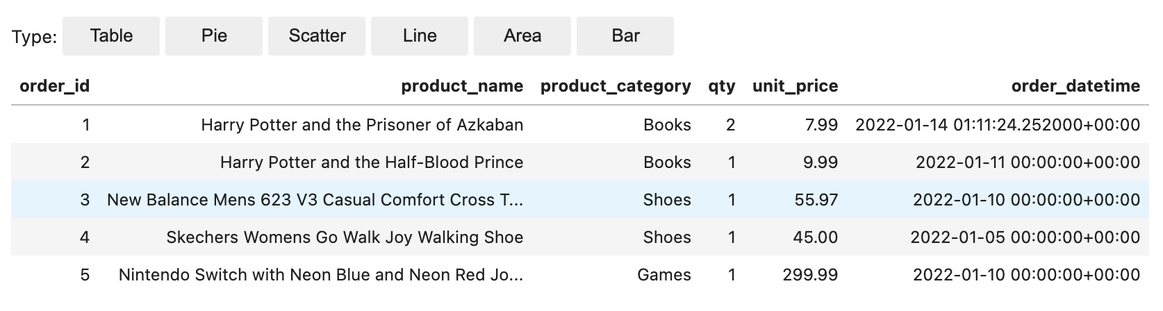
We now insert four more records and then query the orders table and confirm that the five records are present:

SELECT * FROM glue_catalog1.salesdb.orders

Querying from Athena

Because Iceberg on Amazon EMR comes pre-integrated with the AWS Glue Data Catalog, we can now query the Iceberg tables from AWS analytics services that support Iceberg. Let’s query the salesdb/orders table from Athena as shown in the following screenshot.

Upserts

The notebook then gives examples for updates and deletes, and even upserts. We use the MERGE INTO statement for upserts, which uses the source table orders_update with new and updated records:

MERGE INTO glue_catalog1.salesdb.orders target 
USING glue_catalog1.salesdb.orders_update source          
ON target.order_id = source.order_id              
WHEN MATCHED THEN 
    UPDATE SET
        order_id = source.order_id,
        product_name = source.product_name,
        product_category = source.product_category,
        qty = source.qty,
        unit_price = source.unit_price,
        order_datetime = source.order_datetime
WHEN NOT MATCHED THEN
    INSERT *
select * from glue_catalog1.salesdb.orders;

Schema evolution

We then walk through schema evolution using simple ALTER TABLE commands to add, rename, and drop columns. The following example how simple it is to rename a column:

ALTER TABLE glue_catalog1.salesdb.orders RENAME COLUMN qty TO quantity
DESC table glue_catalog1.salesdb.orders

Time travel

Iceberg also allows us to travel backward or forward by storing point-in-time snapshots. We can travel using timestamps when the snapshots were created or directly using the snapshot_id. The following is an example of a CALL statement that uses rollback_to_snapshot:

%%sql
CALL glue_catalog1.system.rollback_to_snapshot('salesdb.orders', 8008410363488501197)

We then travel forward in time by calling set_current_snapshot:

%%sql
CALL glue_catalog1.system.set_current_snapshot('salesdb.orders', 8392090950225782953)

Partition evolution

The notebook ends with an example that shows how partition evolution works in Iceberg. Iceberg stores partition information as part of the metadata. Because there is no separate partition column in the data itself, changing the partitioning scheme to hourly partitions for example is just a matter of calling a different partition transform hours(…) on an existing column order_datetime as shown in the following example:

%%sql
ALTER TABLE glue_catalog1.salesdb.orders ADD PARTITION FIELD hours(order_datetime)

You can continue to use the old partition on the old data. New data is written using the new spec in a new layout. Metadata for each of the partition versions is kept separately.

The notebook shows how you can query the table using the new hourly partition:

%%sql
SELECT * FROM glue_catalog1.salesdb.orders where hour(order_datetime)=1

You can continue to query your old data using the day() transform. There is only the original order_datetime column in the table.

%%sql
SELECT * FROM glue_catalog1.salesdb.orders where day(order_datetime)>=14

You don’t have to store additional columns to accommodate multiple partitioning schemes. The partition definitions are in the metadata, providing the flexibility to evolve and change the partition definitions in the future.

Conclusion

In this post, we introduced Apache Iceberg and explained how Iceberg solves some challenges in modern data lakes. We then walked you through how to run Iceberg on Amazon EMR using the AWS Glue Data Catalog as the metastore, and query the data using Athena. You can also run upserts on this data from Athena. There is no additional cost to using Iceberg with Amazon EMR.

For more information about Iceberg, refer to How Iceberg works. Iceberg on Amazon EMR, with its integration with AWS Analytics services, can simplify the way you process, upsert, and delete data, with full support for ACID transactions in Amazon S3. You can also implement schema evolution, partition evolution, time travel, and compaction of data.


About the Author

Sekar Srinivasan is a Sr. Specialist Solutions Architect at AWS focused on Big Data and Analytics. Sekar has over 20 years of experience working with data. He is passionate about helping customers build scalable solutions modernizing their architecture and generating insights from their data. In his spare time he likes to work on non-profit projects, especially those focused on underprivileged Children’s education.

AWS Week in Review – June 27, 2022

Post Syndicated from Danilo Poccia original https://aws.amazon.com/blogs/aws/aws-week-in-review-june-27-2022/

This post is part of our Week in Review series. Check back each week for a quick roundup of interesting news and announcements from AWS!

It’s the beginning of a new week, and I’d like to start with a recap of the most significant AWS news from the previous 7 days. Last week was special because I had the privilege to be at the very first EMEA AWS Heroes Summit in Milan, Italy. It was a great opportunity of mutual learning as this community of experts shared their thoughts with AWS developer advocates, product managers, and technologists on topics such as containers, serverless, and machine learning.

Participants at the EMEA AWS Heroes Summit 2022

Last Week’s Launches
Here are the launches that got my attention last week:

Amazon Connect Cases (available in preview) – This new capability of Amazon Connect provides built-in case management for your contact center agents to create, collaborate on, and resolve customer issues. Learn more in this blog post that shows how to simplify case management in your contact center.

Many updates for Amazon RDS and Amazon Aurora – Amazon RDS Custom for Oracle now supports Oracle database 12.2 and 18c, and Amazon RDS Multi-AZ deployments with one primary and two readable standby database instances now supports M5d and R5d instances and is available in more Regions. There is also a Regional expansion for RDS Custom. Finally, PostgreSQL 14, a new major version, is now supported by Amazon Aurora PostgreSQL-Compatible Edition.

AWS WAF Captcha is now generally available – You can use AWS WAF Captcha to block unwanted bot traffic by requiring users to successfully complete challenges before their web requests are allowed to reach resources.

Private IP VPNs with AWS Site-to-Site VPN – You can now deploy AWS Site-to-Site VPN connections over AWS Direct Connect using private IP addresses. This way, you can encrypt traffic between on-premises networks and AWS via Direct Connect connections without the need for public IP addresses.

AWS Center for Quantum Networking – Research and development of quantum computers have the potential to revolutionize science and technology. To address fundamental scientific and engineering challenges and develop new hardware, software, and applications for quantum networks, we announced the AWS Center for Quantum Networking.

Simpler access to sustainability data, plus a global hackathon – The Amazon Sustainability Data Initiative catalog of datasets is now searchable and discoverable through AWS Data Exchange. As part of a new collaboration with the International Research Centre in Artificial Intelligence, under the auspices of UNESCO, you can use the power of the cloud to help the world become sustainable by participating to the Amazon Sustainability Data Initiative Global Hackathon.

For a full list of AWS announcements, be sure to keep an eye on the What’s New at AWS page.

Other AWS News
A couple of takeaways from the Amazon re:MARS conference:

Amazon CodeWhisperer (preview) – Amazon CodeWhisperer is a coding companion powered by machine learning with support for multiple IDEs and languages.

Synthetic data generation with Amazon SageMaker Ground Truth – Generate labeled synthetic image data that you can combine with real-world data to create more complete training datasets for your ML models.

Some other updates you might have missed:

AstraZeneca’s drug design program built using AWS wins innovation award – AstraZeneca received the BioIT World Innovative Practice Award at the 20th anniversary of the Bio-IT World Conference for its novel augmented drug design platform built on AWS. More in this blog post.

Large object storage strategies for Amazon DynamoDB – A blog post showing different options for handling large objects within DynamoDB and the benefits and disadvantages of each approach.

Amazon DevOps Guru for RDS under the hood – Some details of how DevOps Guru for RDS works, with a specific focus on its scalability, security, and availability.

AWS open-source news and updates – A newsletter curated by my colleague Ricardo to bring you the latest open-source projects, posts, events, and more.

Upcoming AWS Events
It’s AWS Summits season and here are some virtual and in-person events that might be close to you:

On June 30, the AWS User Group Ukraine is running an AWS Tech Conference to discuss digital transformation with AWS. Join to learn from many sessions including a fireside chat with Dr. Werner Vogels, CTO at Amazon.com.

That’s all from me for this week. Come back next Monday for another Week in Review!

— Danilo

Highlights from Git 2.37

Post Syndicated from Taylor Blau original https://github.blog/2022-06-27-highlights-from-git-2-37/

The open source Git project just released Git 2.37, with features and bug fixes from over 75 contributors, 20 of them new. We last caught up with you on the latest in Git back when 2.36 was released.

To celebrate this most recent release, here’s GitHub’s look at some of the most interesting features and changes introduced since last time.

Before we get into the details of Git 2.37.0, we first wanted to let you know that Git Merge is returning this September. The conference features talks, workshops, and more all about Git and the Git ecosystem. There is still time to submit a proposal to speak. We look forward to seeing you there!

A new mechanism for pruning unreachable objects

In Git, we often talk about classifying objects as either “reachable” or “unreachable”. An object is “reachable” when there is at least one reference (a branch or a tag) from which you can start an object walk (traversing from commits to their parents, from trees into their sub-trees, and so on) and end up at your destination. Similarly, an object is “unreachable” when no such reference exists.

A Git repository needs all of its reachable objects to ensure that the repository is intact. But it is free to discard unreachable objects at any time. And it is often desirable to do just that, particularly when many unreachable objects have piled up, you’re running low on disk space, or similar. In fact, Git does this automatically when running garbage collection.

But observant readers will notice the gc.pruneExpire configuration. This setting defines a “grace period” during which unreachable objects which are not yet old enough to be removed from the repository completely are left alone. This is done in order to mitigate a race condition where an unreachable object that is about to be deleted becomes reachable by some other process (like an incoming reference update or a push) before then being deleted, leaving the repository in a corrupt state.

Setting a small, non-zero grace period makes it much less likely to encounter this race in practice. But it leads us to another problem: how do we keep track of the age of the unreachable objects which didn’t leave the repository? We can’t pack them together into a single packfile; since all objects in a pack share the same modification time, updating any object drags them all forward. Instead, prior to Git 2.37, each surviving unreachable object was written out as a loose object, and the mtime of the individual objects was used to store their age. This can lead to serious problems when there are many unreachable objects which are too new and can’t be pruned.

Git 2.37 introduces a new concept, cruft packs, which allow unreachable objects to be stored together in a single packfile by writing the ages of individual objects in an auxiliary table stored in an *.mtimes file alongside the pack.

While cruft packs don’t eliminate the data race we described earlier, in practice they can help make it much less likely by allowing repositories to prune with a much longer grace period, without worrying about the potential to create many loose objects. To try it out yourself, you can run:

$ git gc --cruft --prune=1.day.ago

and notice that your $GIT_DIR/objects/pack directory will have an additional .mtimes file, storing the ages of each unreachable object written within the last 24 hours

$ ls -1 .git/objects/pack
pack-243103d0f640e0096edb3ef0c842bc5534a9f9a4.idx
pack-243103d0f640e0096edb3ef0c842bc5534a9f9a4.mtimes
pack-243103d0f640e0096edb3ef0c842bc5534a9f9a4.pack
pack-5a827af6f1a793a45c816b05d40dfd4d5f5edf28.idx
pack-5a827af6f1a793a45c816b05d40dfd4d5f5edf28.pack

There’s a lot of detail we haven’t yet covered on cruft packs, so expect a more comprehensive technical overview in a separate blog post soon.

[source]

A builtin filesystem monitor for Windows and macOS

As we have discussed often before, one of the factors that significantly impact Git’s performance is the size of your working directory. When you run git status, for example, Git has to crawl your entire working directory (in the worst case) in order to figure out which files have been modified.

Git has its own cached understanding of the filesystem to avoid this whole-directory traversal in many cases. But it can be expensive for Git to update its cached understanding of the filesystem with the actual state of the disk while you work.

In the past, Git has made it possible to integrate with tools like Watchman via a hook, making it possible to replace Git’s expensive refreshing process with a long-running daemon which tracks the filesystem state more directly.

But setting up this hook and installing a third-party tool can be cumbersome. In Git 2.37, this functionality is built into Git itself on Windows and macOS, removing the need to install an external tool and configure the hook.

You can enable this for your repository by enabling the core.fsmonitor config setting.

$ git config core.fsmonitor true

After setting up the config, an initial git status will take the normal amount of time, but subsequent commands will take advantage of the monitored data and run significantly faster.

The full implementation is impossible to describe completely in this post. Interested readers can follow along later this week with a blog post written by Jeff Hostetler for more information. We’ll be sure to add a link here when that post is published.

[source, source, source, source]

The sparse index is ready for wide use

We previously announced Git’s sparse index feature, which helps speed up Git commands when using the sparse-checkout feature in a large repository.

In case you haven’t seen our earlier post, here’s a brief refresher. Often when working in an extremely large repository, you don’t need the entire contents of your repository present locally in order to contribute. For example, if your company uses a single monorepo, you may only be interested in the parts of that repository that correspond to the handful of products you work on.

Partial clones make it possible for Git to only download the objects that you care about. The sparse index is an equally important component of the equation. The sparse index makes it possible for the index (a key data structure which tracks the content of your next commit, which files have been modified, and more) to only keep track of the parts of your repository that you’re interested in.

When we originally announced the sparse index, we explained how different Git subcommands would have to be updated individually to take advantage of the sparse index. With Git 2.37.0, all of those integrations are now included in the core Git project and available to all users.

In this release, the final integrations were for git show, git sparse-checkout, and git stash. In particular, git stash has the largest performance boost of all of the integrations so far because of how the command reads and writes indexes multiple times in a single process, achieving a near 80% speed-up in certain cases (though see this thread for all of the details).

[source, source, source]

That’s just a sample of changes from the latest release. For more, check out the release notes for 2.37, or any previous version in the Git repository.

Tidbits

Now that we have looked at some of the bigger features in detail, let’s turn to a handful of smaller topics from this release.

  • Speaking of sparse checkouts, this release deprecates the non---cone-mode style of sparse checkout definitions.

    For the uninitiated, the git sparse-checkout command supports two kinds of patterns which dictate which parts of your repository should be checked out: “cone” mode, and “non-cone” mode. The latter, which allows specifying individual files with a .gitignore-style syntax, can be confusing to use correctly, and has performance problems (namely that in the worst case all patterns must try to be matched with all files, leading to slow-downs). Most importantly, it is incompatible with the sparse-index, which brings the performance enhancements of using a sparse checkout to all of the Git commands you’re familiar with.

    For these reasons (and more!), the non---cone mode style of patterns is discouraged, and users are instead encouraged to use --cone mode.

    [source]

  • In our highlights from the last Git release, we talked about more flexible fsync configuration, which made it possible to more precisely define what files Git would explicitly synchronize with fsync() and what strategy it would use to do that synchronization.

    This release brings a new strategy to the list supported by core.fsyncMethod: “batch”, which can provide significant speed-ups on supported filesystems when writing many individual files. This new mode works by staging many updates to the disk’s writeback cache before preforming a single fsync() causing the disk to flush its writeback cache. Files are then atomically moved into place, guaranteeing that they are fsync()-durable by the time they enter the object directory.

    For now, this mode only supports batching loose object writes, and will only be enabled when core.fsync includes the loose-objects value. On a synthetic test of adding 500 files to the repository with git add (each resulting in a new loose object), the new batch mode imposes only a modest penalty over not fsyncing at all.

    On Linux, for example, adding 500 files takes .06 seconds without any fsync() calls, 1.88 seconds with an fsync() after each loose object write, and only .15 seconds with the new batched fsync(). Other platforms display similar speed-ups, with a notable example being Windows, where the numbers are .35 seconds, 11.18 seconds, and just .41 seconds, respectively.

    [source]

  • If you’ve ever wondered, “what’s changed in my repository since yesterday?”, one way you can figure that out is with the --since option, which is supported by all standard revision-walking commands, like log and rev-list.

    This option works by starting with the specified commits, and walking recursively along each commit’s parents, stopping the traversal as soon as it encounters a commit older than the --since date. But in occasional circumstances (particularly when there is) clock skew this can produce confusing results.

    For example, suppose you have three commits, C1, C2, and C3, where C2 is the parent of C3, and C1 is the parent of C2. If both C1 and C3 were written in the last hour, but C2 is a day old (perhaps because the committer’s clock is running slow), then a traversal with --since=1.hour.ago will only show C3, since seeing C2 causes Git to halt its traversal.

    If you expect your repository’s history has some amount of clock skew, then you can use --since-as-filter in place of --since, which only prints commits newer than the specified date, but does not halt its traversal upon seeing an older one.

    [source]

  • If you work with partial clones, and have a variety of different Git remotes, it can be confusing to remember which partial clone filter is attached to which remote.

    Even in a simple example, trying to remember what object filter was used to clone your repository requires this incantation:

    $ git config remote.origin.partialCloneFilter
    

    In Git 2.37, you can now access this information much more readily behind the -v flag of git remote, like so:

    $ git remote -v
    origin    [email protected]:git/git.git (fetch) [tree:0]
    origin    [email protected]:git/git.git (push)
    

    Here, you can easily see between the square-brackets that the remote origin uses a tree:0 filter.

    This work was contributed by Abhradeep Chakraborty, a Google Summer of Code student, who is one of three students participating this year and working on Git.

    [source]

  • Speaking of remote configuration, Git 2.37 ships with support for warning or exiting when it encounters plain-text credentials stored in your configuration with the new transfer.credentialsInUrl setting.

    Storing credentials in plain-text in your repository’s configuration is discouraged, since it forces you to ensure you have appropriately restrictive permissions on the configuration file. Aside from storing the data unencrypted at rest, Git often passes the full URL (including credentials) to other programs, exposing them on systems where other processes have access to arguments list of sensitive processes. In most cases, it is encouraged to use Git’s credential mechanism, or tools like GCM.

    This new setting allows Git to either ignore or halt execution when it sees one of these credentials by setting the transfer.credentialsInUrl to “warn” or “die” respectively. The default, “allow”, does nothing.

    [source, source]

  • If you’ve ever used git add -p to stage the contents of your working tree incrementally, then you may be familiar with git add‘s “interactive mode”, or git add -i, of which git add -p is a sub-mode.

    In addition to “patch” mode, git add -i supports “status”, “update”, “revert”, “add untracked”, “patch”, and “diff”. Until recently, this mode of git add -i was actually written in Perl. This command has been the most recent subject of a long-running effort to port Git commands written in Perl into C. This makes it possible to use Git’s libraries without spawning sub-processes, which can be prohibitively expensive on certain platforms.

    The C reimplementation of git add -i has shipped in releases of Git as early as v2.25.0. In more recent versions, this reimplementation has been in “testing” mode behind an opt-in configuration. Git 2.37 promotes the C reimplementation by default, so Windows users should notice a speed-up when using git add -p.

    [source, source, source, source, source, source, source]

  • Last but not least, there is a lot of exciting work going on for Git developers, too, like improving the localization workflow, improving CI output with GitHub Actions, and reducing memory leaks in internal APIs.

    If you’re interested in contributing to Git, now is a more exciting time than ever to start. Check out this guide for some tips on getting started.

The rest of the iceberg

That’s just a sample of changes from the latest release. For more, check out the release notes for 2.37 or any previous version in the Git repository.

Building a low-code speech “you know” counter using AWS Step Functions

Post Syndicated from Julian Wood original https://aws.amazon.com/blogs/compute/building-a-low-code-speech-you-know-counter-using-aws-step-functions/

This post is written by Doug Toppin, Software Development Engineer, and Kishore Dhamodaran, Solutions Architect.

In public speaking, filler phrases can distract the audience and reduce the value and impact of what you are telling them. Reviewing recordings of presentations can be helpful to determine whether presenters are using filler phrases. Instead of manually reviewing prior recordings, automation can process media files and perform a speech-to-text function. That text can then be processed to report on the use of filler phrases.

This blog explains how to use AWS Step Functions, Amazon EventBridge, Amazon Transcribe and Amazon Athena to report on the use of the common phrase “you know” in media files. These services can automate and reduce the time required to find the use of filler phrases.

Step Functions can automate and chain together multiple activities and other Amazon services. Amazon Transcribe is a speech to text service that uses media files as input and produces textual transcripts from them. Athena is an interactive query service that makes it easier to analyze data in Amazon S3 using standard SQL. Athena enables the use of standard SQL to query data in S3.

This blog shows a low-code, configuration driven approach to implementing this solution. Low-code means writing little or no custom software to perform a function. Instead, you use a configuration drive approach using service integrations where state machine tasks call AWS services using existing SDKs, APIs, or interfaces. A configuration driven approach in this example is using Step Functions’ Amazon States Language (ASL) to tie actions together rather than writing traditional code. This requires fewer details for data management and error handling combined with a visual user interface for composing the workflow. As the actions and logic are clearly defined with the visual workflow, this reduces maintenance.

Solution overview

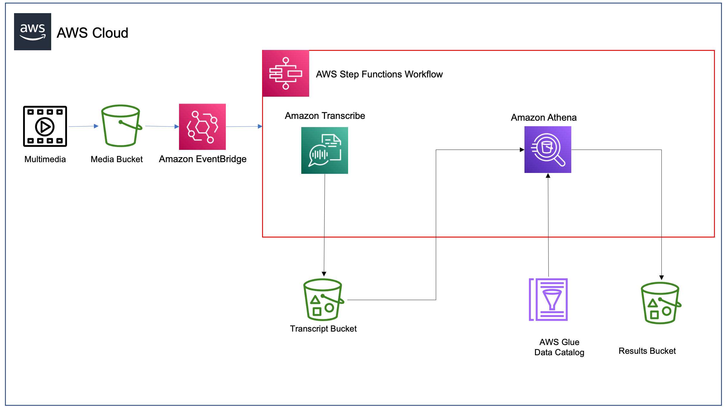
The following diagram shows the solution architecture.

SolutionOverview

Solution Overview

  1. You upload a media file to an Amazon S3 Media bucket.
  2. The media file upload to S3 triggers an EventBridge rule.
  3. The EventBridge rule starts the Step Functions state machine execution.
  4. The state machine invokes Amazon Transcribe to process the media file.
  5. The transcription output file is stored in the Amazon S3 Transcript bucket.
  6. The state machine invokes Athena to query the textual transcript for the filler phrase. This uses the AWS Glue table to describe the format of the transcription results file.
  7. The filler phrase count determined by Athena is returned and stored in the Amazon S3 Results bucket.

Prerequisites

  1. An AWS account and an AWS user or role with sufficient permissions to create the necessary resources.
  2. Access to the following AWS services: Step Functions, Amazon Transcribe, Athena, and Amazon S3.
  3. Latest version of the AWS Serverless Application Model (AWS SAM) CLI, which helps developers create and manage serverless applications in the AWS Cloud.
  4. Test media files (for example, the Official AWS Podcast).

Example walkthrough

  1. Clone the GitHub repository to your local machine.
  2. git clone https://github.com/aws-samples/aws-stepfunctions-examples.git
  3. Deploy the resources using AWS SAM. The deploy command processes the AWS SAM template file to create the necessary resources in AWS. Choose you-know as the stack name and the AWS Region that you want to deploy your solution to.
  4. cd aws-stepfunctions-examples/sam/app-low-code-you-know-counter/
    sam deploy --guided

Use the default parameters or replace with different values if necessary. For example, to get counts of a different filler phrase, replace the FillerPhrase parameter.

GlueDatabaseYouKnowP Name of the AWS Glue database to create.
AthenaTableName Name of the AWS Glue table that is used by Athena to query the results.
FillerPhrase The filler phrase to check.
AthenaQueryPreparedStatementName Name of the Athena prepared statement used to run SQL queries on.
AthenaWorkgroup Athena workgroup to use
AthenaDataCatalog The data source for running the Athena queries
SAM Deploy

SAM Deploy

Running the filler phrase counter

  1. Navigate to the Amazon S3 console and upload an mp3 or mp4 podcast recording to the bucket named bucket-{account number}-{Region}-you-know-media.
  2. Navigate to the Step Functions console. Choose the running state machine, and monitor the execution of the transcription state machine.
  3. State Machine Execution

    State Machine Execution

  4. When the execution completes successfully, select the QueryExecutionSuccess task to examine the output and see the filler phrase count.
  5. State Machine Output

    State Machine Output

  6. Amazon Transcribe produces the transcript text of the media file. You can examine the output in the Results bucket. Using the S3 console, navigate to the bucket, choose the file matching the media file name and use ‘Query with S3 Select’ to view the content.
  7. If the transcription job does not execute, the state machine reports the failure and exits.
  8. State Machine Fail

    State Machine Fail

Exploring the state machine

The state machine orchestrates the transcription processing:

State Machine Explore

State Machine Explore

The StartTranscriptionJob task starts the transcription job. The Wait state adds a 60-second delay before checking the status of the transcription job. Until the status of the job changes to FAILED or COMPLETED, the choice state continues.

When the job successfully completes, the AthenaStartQueryExecutionUsingPreparedStatement task starts the Athena query, and stores the results in the S3 results bucket. The AthenaGetQueryResults task retrieves the count from the resultset.

The TranscribeMediaBucket holds the media files to be uploaded. The configuration sends the upload notification event to EventBridge:

      
   NotificationConfiguration:
     EventBridgeConfiguration:
       EventBridgeEnabled: true
	  

The TranscribeResultsBucket has an associated policy to provide access to Amazon Transcribe. Athena stores the output from the queries performed by the state machine in the AthenaQueryResultsBucket .

When a media upload occurs, the YouKnowTranscribeStateMachine uses Step Functions’ native event integration to trigger an EventBridge rule. This contains an event object similar to:

{
  "version": "0",
  "id": "99a0cb40-4b26-7d74-dc59-c837f5346ac6",
  "detail-type": "Object Created",
  "source": "aws.s3",
  "account": "012345678901",
  "time": "2022-05-19T22:21:10Z",
  "region": "us-east-2",
  "resources": [
    "arn:aws:s3:::bucket-012345678901-us-east-2-you-know-media"
  ],
  "detail": {
    "version": "0",
    "bucket": {
      "name": "bucket-012345678901-us-east-2-you-know-media"
    },
    "object": {
      "key": "Podcase_Episode.m4a",
      "size": 202329,
      "etag": "624fce93a981f97d85025e8432e24f48",
      "sequencer": "006286C2D604D7A390"
    },
    "request-id": "B4DA7RD214V1QG3W",
    "requester": "012345678901",
    "source-ip-address": "172.0.0.1",
    "reason": "PutObject"
  }
}

The state machine allows you to prepare parameters and use the direct SDK integrations to start the transcription job by calling the Amazon Transcribe service’s API. This integration means you don’t have to write custom code to perform this function. The event triggering the state machine execution contains the uploaded media file location.

  StartTranscriptionJob:
	Type: Task
	Comment: Start a transcribe job on the provided media file
	Parameters:
	  Media:
		MediaFileUri.$: States.Format('s3://{}/{}', $.detail.bucket.name, $.detail.object.key)
	  TranscriptionJobName.$: "$.detail.object.key"
	  IdentifyLanguage: true
	  OutputBucketName: !Ref TranscribeResultsBucket
	Resource: !Sub 'arn:${AWS::Partition}:states:${AWS::Region}:${AWS::AccountId}:aws-sdk:transcribe:startTranscriptionJob'

The SDK uses aws-sdk:transcribe:getTranscriptionJob to get the status of the job.


  GetTranscriptionJob:
	Type: Task
	Comment: Retrieve the status of an Amazon Transcribe job
	Parameters:
	  TranscriptionJobName.$: "$.TranscriptionJob.TranscriptionJobName"
	Resource: !Sub 'arn:${AWS::Partition}:states:${AWS::Region}:${AWS::AccountId}:aws-sdk:transcribe:getTranscriptionJob'
	Next: TranscriptionJobStatus

The state machine uses a polling loop with a delay to check the status of the transcription job.


  TranscriptionJobStatus:
	Type: Choice
	Choices:
	- Variable: "$.TranscriptionJob.TranscriptionJobStatus"
	  StringEquals: COMPLETED
	  Next: AthenaStartQueryExecutionUsingPreparedStatement
	- Variable: "$.TranscriptionJob.TranscriptionJobStatus"
	  StringEquals: FAILED
	  Next: Failed
	Default: Wait

When the transcription job completes successfully, the filler phrase counting process begins.

An Athena prepared statement performs the query with the transcription job name as a runtime parameter. The AWS SDK starts the query and the state machine execution pauses, waiting for the results to return before progressing to the next state:

athena:startQueryExecution.sync

When the query completes, Step Functions uses the SDK integration to retrieve the results using athena:getQueryResults:

athena:getQueryResults

It creates an Athena prepared statement to pass the transcription jobname as a parameter for the query execution:

  ResultsQueryPreparedStatement:
    Type: AWS::Athena::PreparedStatement
    Properties:
      Description: Create a statement that allows the use of a parameter for specifying an Amazon Transcribe job name in the Athena query
      QueryStatement: !Sub >-
        select cardinality(regexp_extract_all(results.transcripts[1].transcript, '${FillerPhrase}')) AS item_count from "${GlueDatabaseYouKnow}"."${AthenaTableName}" where jobname like ?
      StatementName: !Ref AthenaQueryPreparedStatementName
      WorkGroup: !Ref AthenaWorkgroup

There are several opportunities to enhance this tool. For example, adding support for multiple filler phrases. You could build a larger application to upload media and retrieve the results. You could take advantage of Amazon Transcribe’s real-time transcription API to display the results while a presentation is in progress to provide immediate feedback to the presenter.

Cleaning up

  1. Navigate to the Amazon Transcribe console. Choose Transcription jobs in the left pane, select the jobs created by this example, and choose Delete.
  2. Cleanup Delete

    Cleanup Delete

  3. Navigate to the S3 console. In the Find buckets by name search bar, enter “you-know”. This shows the list of buckets created for this example. Choose each of the radio buttons next to the bucket individually and choose Empty.
  4. Cleanup S3

    Cleanup S3

  5. Use the following command to delete the stack, and confirm the stack deletion.
  6. sam delete

Conclusion

Low-code applications can increase developer efficiency by reducing the amount of custom code required to build solutions. They can also enable non-developer roles to create automation to perform business functions by providing drag-and-drop style user interfaces.

This post shows how a low-code approach can build a tool chain using AWS services. The example processes media files to produce text transcripts and count the use of filler phrases in those transcripts. It shows how to process EventBridge data and how to invoke Amazon Transcribe and Athena using Step Functions state machines.

For more serverless learning resources, visit Serverless Land.

[$] Two memory-tiering patch sets

Post Syndicated from original https://lwn.net/Articles/898766/

Once upon a time, computers just had one type memory, so memory within
a given system was interchangeable. The arrival of non-uniform
memory access (NUMA) systems complicated the situation significantly; now
some memory was faster to access than the rest, and memory-management
algorithms had to adapt or performance would suffer. But NUMA was just the
start; today’s tiered-memory systems, which may include several tiers of
memory with different performance characteristics, are adding new
challenges. A couple of relevant patch sets currently under review help to
illustrate the types of problems that will have to be solved.

KDE Apps Mid-Year Update (KDE.news)

Post Syndicated from original https://lwn.net/Articles/899167/

Here’s an
update on recent KDE application development
on KDE.news:

KStars is probably the most feature-rich free astronomy software around and the 3.5.9
release adds some exciting new features.

HiPS (Hierarchical Progressive Surveys) is a technology that provides
progressive high resolution images of the sky at different zoom
levels. KStars fully supports online HiPS where data is downloaded from
online servers and cached to be displayed on the Sky Map.

Ojeda: Memory Safety for the World’s Largest Software Project

Post Syndicated from original https://lwn.net/Articles/899164/

Miguel Ojeda has posted an
update on the Rust-for-Linux project
.

This second year since the RFC we are looking forward to several
milestones which hopefully we will achieve:

  • More users or use cases inside the kernel, including example drivers – this is pretty important to get merged into the kernel.
  • Splitting the kernel crate and managing dependencies to allow better development.
  • Extending the current integration of the kernel documentation, testing and other tools.
  • Getting more subsystem maintainers, companies and researchers involved.
  • Seeing most of the remaining Rust features stabilized.
  • Possibly being able to start compiling the Rust code in the kernel with GCC.
  • And, of course, getting merged into the mainline kernel, which
    should make everything else easier!

API Security: Best Practices for a Changing Attack Surface

Post Syndicated from Ray Cochrane original https://blog.rapid7.com/2022/06/27/api-security-best-practices-for-a-changing-attack-surface/

API Security: Best Practices for a Changing Attack Surface

API usage is skyrocketing. According to the latest State of the API Report, API requests increased by 56% last year to a total of 855 million, and Google says the growth isn’t expected to slow any time soon.

APIs – short for application programming interfaces – are a critical component of how applications are built. They control the type of requests that occur between programs, how requests are made, and the format of those requests.

The huge increase in usage stems from the important role APIs – and web applications more broadly – play in digital transformation. APIs have helped facilitate the transition from monolithic applications to microservices. They’ve enabled businesses to provide user-oriented API-based services for B2B use cases, including automation and integration. And they’re integral to modern web applications, which are no longer just HTML with links but rich user interfaces, built as single-page apps with REST API backends. Nearly every modern application utilizes – or is – an API.
Today, it’s almost impossible to do anything online without interacting with an API. That’s why cyberattacks are increasingly targeting APIs, and they’ve become a large part of the application attack surface.

Why securing APIs is important

APIs are a lucrative target that can allow hackers to gain access to an otherwise secure system and exploit vulnerabilities. Not only do APIs often suffer from the same vulnerabilities as web applications – like broken access controls, injections, security misconfigurations, and vulnerabilities inherited from other dependent code libraries – but they are also more susceptible to resource consumption and rate limiting issues due to the automated nature of their users.

Due to a lack of knowledge in the market, it’s also common that legacy issues from early APIs are carried forward. For example, not all APIs will be fronted by an API gateway, with older APIs sitting in the background with little or no protection simply due to a lack of awareness of them. Many unused APIs will also not have been decommissioned, as newer APIs are produced and replace them as a product evolves, due to a lack of standard process and bad practice. This can leave legacy APIs vulnerable to attacks.

How to secure an API

The first step in securing your APIs is to audit your environment and/or applications to take an inventory of what APIs you have and which ones you’re actually utilizing. Then, you must understand the purpose of each individual API to allow you to validate that it is working as expected. You must also understand the expected behavior of the API to allow identification of threats more readily by being able to capture abnormal activity. Once you have a firm understanding of what the API’s functionality is and what expected behavior is, you can then both manage and test your API more effectively and efficiently.

API management is a key element for API security. APIs not only require the same controls as web apps but also additional controls specific to the API’s unique function. Documentation and version control of APIs is of vital importance, as one product can have multiple APIs – even hundreds or thousands.

Poor management can lead to issues with legacy and defunct APIs, as you will often find that only a small portion of APIs pass through an API gateway. Meanwhile, older APIs – which haven’t been decommissioned, or which teams simply aren’t aware of – can sit in the background with no protection. The probability of known vulnerabilities with older APIs is also significantly higher, which amplifies the risk profile.

The same legacy issues can also lead to coverage gaps, and calls that are outside of an API gateway could leave a blind spot when it comes to intra-API calls. Publishing and clearly defining your API will simplify users’ understanding of the API, allowing them to connect in the most appropriate and effective way. Ensuring your API is appropriately monitored is a key management technique. Continuously undertaking performance checks will allow you to understand if the API is under stress from being overloaded. It can also provide an indication of traffic volumes to monitor usage, potentially gauge malicious activity (via audit logs), and judge whether you need to scale up your operation. Lastly, having a response plan in place for attacks is a vital control in API security, allowing for a rapid but controlled response to potential threats.


There have been many recent examples of API-based attacks, such as those experienced by WordPress – and even on the dating scene with Bumble’s recent vulnerability issues. Some simple but effective steps you can take to secure your API and reduce the risk of such exposures include:

  • Authentication: Do you have a control in place to understand who’s calling your API?
  • Authorization: Should the person calling be able to access this data?
  • Encryption: Have you encrypted your network traffic?
  • Traffic management: Have you set rate limits or thresholds to keep a customer from pulling too much data or running scripts to tie up an API?
  • Audit logging: Effective logging ensures you can understand what normal traffic looks like and allows you to identify abnormal activity.

How to test your API

API testing is still evolving to keep up with the increase in volume and complexity. While manual API security testing can be done with traditional testing tools, and fully automated API security testing is partially supported by most major DAST solutions, there are many open-source tools written for guided API security testing. API testing used in conjunction with proper API management will increase API security.

API testing is most effective when you have a full risk profile of your business – i.e. you are fully aware of all of your APIs (including legacy or defunct APIs) to ensure you have no blindspots that could be exposed or manipulated. Taking time to identify vulnerabilities in API frameworks, your network, configuration, and policy all enhance your API security.

Anticipating threats by understanding expected behavior and having adequate testing in place will allow for proactive coverage and enhanced protection and threat identification.

Finally, you must continuously test your endpoint to ensure protection is maintained at all times and optimum security is in place. The ability to identify and block security risks before they occur is vital in the fight to provide the best protection against threats to your API.

Additional reading:

NEVER MISS A BLOG

Get the latest stories, expertise, and news about security today.

Orchestrating AWS Glue crawlers using AWS Step Functions

Post Syndicated from Benjamin Smith original https://aws.amazon.com/blogs/compute/orchestrating-aws-glue-crawlers-using-aws-step-functions/

This blog post is written by Justin Callison, General Manager, AWS Workflow.

Organizations generate terabytes of data every day in a variety of semistructured formats. AWS Glue and Amazon Athena can give you a simpler and more cost-effective way to analyze this data with no infrastructure to manage. AWS Glue crawlers identify the schema of your data and manage the metadata required to analyze the data in place, without the need to transform this data and load into a data warehouse.

The timing of when your crawlers run and complete is important. You must ensure the crawler runs after your data has updated and before you query it with Athena or analyze with an AWS Glue job. If not, your analysis may experience errors or return incomplete results.

In this blog, you learn how to use AWS Step Functions, a low-code visual workflow service that integrates with over 220 AWS services. The service orchestrates your crawlers to control when they start, confirm completion, and combine them into end-to-end, serverless data processing workflows.

Using Step Functions to orchestrate multiple AWS Glue crawlers, provides a number of benefits when compared to implementing a solution directly with code. Firstly, the workflow provides an instant visual understanding of the application, and any errors that might occur during execution. Step Functions’ ability to run nested workflows inside a Map state helps to decouple and reuse application components with native array iteration. Finally, the Step Functions wait state lets the workflow periodically poll the status of the crawl job, without incurring additional cost for idol wait time.

Deploying the example

With this example, you create three datasets in Amazon S3, then use Step Functions to orchestrate AWS Glue crawlers to analyze the datasets and make them available to query using Athena.

You deploy the example with AWS CloudFormation using the following steps:

  1. Download the template.yaml file from here.
  2. Log in to the AWS Management Console and go to AWS CloudFormation.
  3. Navigate to Stacks -> Create stack and select With new resources (standard).
  4. Select Template is ready and Upload a template file, then Choose File and select the template.yaml file that you downloaded in Step 1 and choose Next.
  5. Enter a stack name, such as glue-stepfunctions-demo, and choose Next.
  6. Choose Next, check the acknowledgement boxes in the Capabilities and transforms section, then choose Create stack.
  7. After deployment, the status updates to CREATE_COMPLETE.

Create your datasets

Navigate to Step Functions in the AWS Management Console and select the create-dataset state machine from the list. This state machine uses Express Workflows and the Parallel state to build three datasets concurrently in S3. The first two datasets include information by user and location respectively and include files per day over the 5-year period from 2016 to 2020. The third dataset is a simpler, all-time summary of data by location.

To create the datasets, you choose Start execution from the toolbar for the create-dataset state machine, then choose Start execution again in the dialog box. This runs the state machine and creates the datasets in S3.

Navigate to the S3 console and view the glue-demo-databucket created for this example. In this bucket, in a folder named data, there are three subfolders, each containing a dataset.

The all-time-location-summaries folder contains a set of JSON files, one for each location.

The daily-user-summaries and daily-location-summaries contain a folder structure with nested folders for each year, month, and date. In addition to making this data easier to navigate via the console, this folder structure provides hints to AWS Glue that it can use to partition this dataset and make it more efficient to query.

Crawling

You now use AWS Glue crawlers to analyze these datasets and make them available to query. Navigate to the AWS Glue console, select Crawlers to see the list of Crawlers that you created when you deployed this example. Select the daily-user-summaries crawler to view details and note that they have tags assigned to indicate metadata such as the datatype of the data and whether the dataset is-partitioned.

Now, return to the Step Functions console and view the run-crawlers-with-tags state machine. This state machine uses AWS SDK service integrations to get a list of all crawlers matching the tag criteria you enter. It then uses the map state and the optimized service integration for Step Functions to execute the run-crawler state machine for each of the matching crawlers concurrently. The run-crawler state machine starts each crawler and monitors status until the crawler completes. Once each of the individual crawlers have completed, the run-crawlers-with-tags state machine also completes.

To initiate the crawlers:

  1. Choose Start execution from the top of the page when viewing the run-crawlers-with-tags state machine
  2. Provide the following as Input
    {"tags": {"datatype": "json"}}
  3. Choose Start execution.

After 2-3 minutes, the execution finishes with a Succeeded status once all three crawlers have completed. During this time, you can navigate to the run-crawler state machine to view the individual, nested executions per crawler or to the AWS Glue console to see the status of the crawlers.

Querying the data using Amazon Athena

Now, navigate to the Athena console where you can see the database and tables created by your crawlers. Note that AWS Glue recognized the partitioning scheme and included fields for year, month, and date in addition to user and usage fields for the data contained in the JSON files.

If you have not used Athena in this account before, you see a message instructing you to set a query result location. Choose View settings -> Manage -> Browse S3 and select the athena-results bucket that you created when you deployed the example. Choose Save then return to the Editor to continue.

You can now run queries such as the following, to calculate the total usage for all users over 5 years.

SELECT SUM(usage) all_time_usage FROM “daily_user_summaries”

You can also add filters, as shown in the following example, which limit results to those from 2016.

SELECT SUM(usage) all_time_usage FROM “daily_user_summaries” WHERE year = ‘2016’

Note this second query scanned only 17% as much data (133 KB vs 797 KB) and completed faster. This is because Athena used the partitioning information to avoid querying the full dataset. While the differences in this example are small, for real-world datasets with terabytes of data, your cost and latency savings from partitioning data can be substantial.

The disadvantage of a partitioning scheme is that new folders are not included in query results until you add new partitions. Re-running your crawler identifies and adds the new partitions and using Step Functions to orchestrate these crawlers makes that task simpler.

Extending the example

You can use these example state machines as they are in your AWS accounts to manage your existing crawlers. You can use Amazon S3 event notifications with Amazon EventBridge to trigger crawlers based on data changes. With the Optimized service integration for Amazon Athena, you can extend your workflows to execute queries against these crawled datasets. And you can use these examples to integrate crawler execution into your end-to-end data processing workflows, creating reliable, auditable workflows from ingestion through to analysis.

Conclusion

In this blog post, you learn how to use Step Functions to orchestrate AWS Glue crawlers. You deploy an example that generates three datasets, then uses Step Functions to start and coordinate crawler runs that analyze this data and make it available to query using Athena.

To learn more about Step Functions, visit Serverless Land.

Security updates for Monday

Post Syndicated from original https://lwn.net/Articles/899158/

Security updates have been issued by Debian (openssl), Fedora (dotnet6.0, mediawiki, and python2.7), Mageia (389-ds-base, chromium-browser-stable, exo, and libtiff), Oracle (httpd:2.4 and microcode_ctl), SUSE (dbus-broker, drbd, kernel, liblouis, mariadb, openssl, openssl-1_1, openSUSE kernel modules, oracleasm, php7, php72, python39, salt, and wdiff), and Ubuntu (linux, linux-hwe, mozjs91, and vim).

New partner program for SMB agencies & hosting partners now in closed beta

Post Syndicated from Dan Hollinger original https://blog.cloudflare.com/self-serve-partners-beta/

New partner program for SMB agencies & hosting partners now in closed beta

A fundamental principle here at Cloudflare has always been that we want to serve everyone – from individual developers to small businesses to large corporations. In the earliest days, we provided services to hosting partners and resellers around the globe, who helped bring Cloudflare to thousands of domains with free caching and DDoS protection for shared infrastructures.

Today, we want to reinforce our commitment to our hosting ecosystem and small business partners that leverage Cloudflare to help bring a better Internet experience to their customers. We’ve been building a robust multi-tenant partner platform that we will begin to open up to everyone searching for a faster, safer, and better Internet experience. This platform will come in the form of a Self Serve Partner program that will allow SMB agencies & hosting partners to create accounts for all their customers under one dashboard, consolidate billing, and provide discounted plans to our partners.

Deprecation of our legacy APIs

To make way for the new, we first must discuss the end-of-life of some of Cloudflare’s earliest APIs. Built and launched in 2011, our Hosting and Optimized Partner Programs allowed our initial CDN and DDoS solutions to expand to brand-new audiences around the globe. These APIs were essential for fueling growth in the earliest days of Cloudflare supporting reseller partners, hosting partners, and external plugins that helped make implementing Cloudflare easier than ever.
On November 1, 2022 – Cloudflare will be discontinuing support for our Host and Reseller APIs. After this date:

  • Management of zones, users, and configurations via the Host or Reseller API will be disabled.
  • Any plugins leveraging these APIs will no longer be functional. This includes our legacy cPanel, Plesk and WHMCS plugins. We recommend partners and users begin to work directly within the Cloudflare dashboard for any future configuration management.
  • Any domains created by these APIs will continue to function and traffic will not be impacted after the depreciation period. Customer traffic will not be impacted during the deprecation, and we’ve been working closely with our partners to ensure these domains are transitioned to customer-management where preferred or migrated when appropriate to the new partner platform.
  • Any active specialized subscriptions will be mapped to our current zone plans.
    We are grateful for all of our earliest partners that trusted Cloudflare to increase the security and improve performance for their customer’s domains. All of our partners still leveraging our APIs should have received a communication with our deprecation schedule and next steps. And if there are any additional questions, they can be directed to [email protected].
New partner program for SMB agencies & hosting partners now in closed beta

Our New Partner Platform

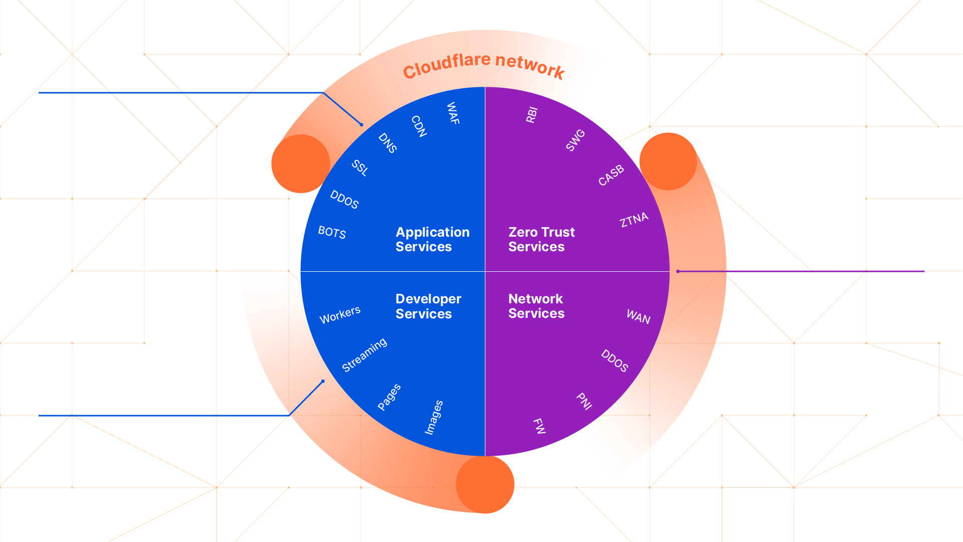
As our solution offering and network grew, these early APIs were not well-equipped to scale with them. Cloudflare has continued to grow its network to over 275 cities and expand well beyond just web performance and security. With a full portfolio of Application Services, Zero Trust Services, Developer and Network solutions, our specialized plans and APIs quickly began to limit our partners instead of empowering them. Cloudflare announced our revamped partner platform a few years ago, and it has since been used with some of our largest integration and service partners supporting our newest SASE and Zero Trust offerings.

Self-serve partnerships in closed beta

With the deprecation of our legacy APIs, we are opening up our Partner Platform to a broader base of partners with a Self-Serve Partner program. Working in tandem with our Self-Serve teams, we’ve been ramping up initial test partners since late last year. Now, we’re excited to announce a path forward for agencies, regional MSPs, and hosting providers that still rely on Cloudflare to help their customers experience a better, faster, and safer Internet:

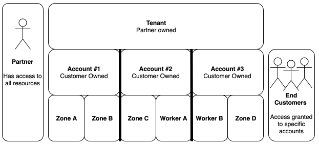
  • Multi-Tenant Account Support
    • Partners will have the ability to create individual customer accounts and manage individual user access to each one from our dashboard or via our Tenant API.
  • Centralized Self-Serve Billing
    • Partners will have the ability to own self-serve billing across each account with a single billing profile, ensuring subscription management is seamless across every account.

New partner program for SMB agencies & hosting partners now in closed beta

  • Access to full catalog of Cloudflare Self-Serve Products & Add-Ons
    • Every feature and add-on that Cloudflare has built will now be available to self-serve partners via the dashboard and API. End-customers will be able to implement load-balancing, Spectrum for TCP/UDP applications, and Workers for deploying code at the edge. Our partner platform ensures partners and customers are getting the most of their Cloudflare solution.
  • Self-Service Plan Discounting
    • We want to reward our partners for working with us and developing expertise across our solution. As part of our program commitments, we are offering volume discounts across all subscription renewals.
  • No Upfront Commitments
    • We’ve heard from many of you that you enjoy working with Cloudflare, but cannot support some minimums for our Enterprise partner programs. This program is built to help you get started, with no upfront commitments for qualified partners.

Comparing our partner programs

Self-Serve Partner Program New Cloudflare One Partner Program Enterprise Reseller & Services Program
Status Closed Beta Early Access General Access
Tiers N/A N/A Select Advanced Elite
Discount Beta Discount – 20% 25-50% 30-40%
Revenue Commitment No No Yes
Training & Enablement Self-Serve Cloudflare University Specialized Training Cloudflare University Specialized Training In-Person Training
Partner Account Resources No – Self Serve Yes – Tier Dependent Yes – Tier Dependent

Sign Up Now

If you want to start using our partner platform, sign up for the closed beta: we plan to start enabling access throughout this year. We’re looking forward to collecting feedback from each of you and learning how we can improve your end-customers experience with our global platform.

Ain’t seen nothing yet…

Cloudflare’s mission is to help build a better Internet. We know we cannot do that alone, and we treasure all of our partners that have worked with us to accomplish that mission across our technical, channel and alliance relationships. Throughout 2022 and 2023, we look to continue to grow our Partner Platform across a few key areas to make it easier to use and seamless to integrate into your current offering across CDN, DDoS, Zero Trust, Workers and more.

  • Enhanced Partner Dashboard
  • Expanded Zero Trust Bundles for Partners
  • Additional Partner Service Opportunities
  • Select training and other Partner-only benefits

More Information:

Become an Enterprise Partner: Partner Portal

Sign Up for the Self-Serve Partner Program

Reach out to [email protected]

Network performance update: Cloudflare One Week June 2022

Post Syndicated from David Tuber original https://blog.cloudflare.com/network-performance-update-cloudflare-one-week-june-2022/

Network performance update: Cloudflare One Week June 2022

Network performance update: Cloudflare One Week June 2022

In September 2021, we shared extensive benchmarking results of 1,000 networks all around the world. The results showed that on a range of tests (TCP connection time, time to first byte, time to last byte), and on different measures (p95, mean), Cloudflare was the fastest provider in 49% of the top 1,000 networks around the world.

Since then, we’ve expanded our testing to cover not just 1,000 but 3,000 networks, and we’ve worked to continuously improve performance, with the ultimate goal of being the fastest everywhere and an intermediate goal to grow the number of networks where we’re the fastest by at least 10% every Innovation Week. We met that goal Platform Week May 2022), and we’re carrying the work over to Cloudflare One Week (June 2022).

We’re excited to share that Cloudflare has the fastest provider in 1,290 of the top 3,000 most reported networks, up from 1,280 even one month ago during Platform Week.

Measuring what matters

To quantify global network performance, we have to get enough data from around the world, across all manner of different networks, comparing ourselves with other providers. We use Real User Measurements (RUM) to fetch a 100kB file from different providers. Users around the world report the performance of different providers.

The more users who report the data, the higher fidelity the signal is. The goal is to provide an accurate picture of where different providers are faster, and more importantly, where Cloudflare can improve. You can read more about the methodology in the original Speed Week blog post here.

Latest data on network performance

Here’s how the breakdown of the fastest networks looked during Platform Week (May 2022):

Network performance update: Cloudflare One Week June 2022

Here’s how that graph looks now during Cloudflare One Week (June 2022):

Network performance update: Cloudflare One Week June 2022

In addition to being the fastest across popular networks, Cloudflare is also committed to being the fastest provider in every country.

Here’s how the map of the fastest provider by country looked during Platform Week (May 2022):

Network performance update: Cloudflare One Week June 2022

And here’s how that map looks during Cloudflare One Week (June 2022):

Network performance update: Cloudflare One Week June 2022

Cloudflare became faster in more Eastern European countries during this time specifically.

Network performance in a Zero Trust world

A zero trust provider needs to not only secure your users on the public Internet, but it also needs to optimize the public Internet. Moving to Zero Trust doesn’t just reduce the need for corporate networks, it also allows user traffic to flow to resources more naturally.

However, given your Zero Trust provider is going to be the gatekeeper for all your users and all your applications, performance is a critical aspect to evaluate Cloudflare is constantly improving our network to ensure that users always have the best experience, and this comes not just from routing fixes, but also through expanding peering arrangements and adding new locations.

This tireless effort helps make us faster in more networks than anyone else, and allows us to deliver all of our services with high performance that customers expect. We know many organizations are just starting their Zero Trust journey, and that a priority of that project is to improve user experience, and we’re excited to keep obsessing over the performance in our network to make sure your teams have a seamless experience in any location.

Interested in learning more about how our Zero Trust products benefit from these improvements? Check out the full roster of our announcements from Cloudflare One Week.

Identifying content gaps in our documentation

Post Syndicated from Cloudflare original https://blog.cloudflare.com/identifying-content-gaps/

Identifying content gaps in our documentation

Identifying content gaps in our documentation

If you’ve tuned into this blog for long enough, you’ll notice that we’re pretty big on using and stress-testing our own products (“dogfooding”) at Cloudflare.

That applies to our security team, product teams, and – as my colleague Kristian just blogged about – even our documentation team. We’re incredibly excited to be on the Pages platform, both because of the performance and workflow improvements and the opportunity to help the platform develop.

What you probably haven’t heard about is how our docs team uses dogfooding – and data – to improve our documentation.

Dogfooding for docs

As a technical writer, it’s pretty common to do the thing you’re documenting. After all, it’s really hard to write step-by-step instructions if you haven’t been through those steps. It’s also a great opportunity to provide feedback to our product teams.

What’s not as common for a writer, however, is actually using the thing you’re documenting. And it’s totally understandable why. You’re already accountable to your deadlines and product managers, so you might not have the time. You might not have the technical background. And then there’s the whole problem of a real-world use case. If you’re really dedicated, you can set up a personal project… but it’s hard to replicate real-world situations and even harder to simulate real-world motivation.

And that brings me to one of the coolest parts of our docs team. We actually manage the Cloudflare settings for our docs website, developers.cloudflare.com. There’s technical oversight from other teams as needed, but that means we’ve directly been involved in:

When we use our own products, it makes us part of the user journey. We know quite viscerally what it’s like when you accidentally break an internal tool with Bot management… because we’ve done it (and profusely apologized!). We know what it’s like to spend a few hours crafting a Transform Rule and realize that – for a specific use case involving search engine crawlers – we needed a Forwarding Page Rule instead.

Identifying content gaps in our documentation

Using our own products gives us a chance to dogfood our docs as well. We realized that we needed to add a page to the 1.1.1.1 docs because several of us set it up on our home devices and didn’t know whether it was working or not. Same thing with the Cloudflare Tunnel docs. When we use the thing, it’s easier for us to help others use it too.

Data for docs

Beyond our own experience – and even beyond the feedback we get through our open-source content strategy – we also look at quantitative data to identify gaps and potential improvements in our docs.

One of the easiest ways to identify gaps is to look at internal search data. When folks are searching from within our docs, are they leaving to view pages within other Cloudflare content sources (Community, Learning Center, etc.)? And does that page conceptually belong in our docs? We’ve used those two questions to identify and correct several gaps in our documentation, such as new pages on creating subdomain records, Cloudflare Ray IDs, and more.

External search data also informs our content strategy. When folks are coming into Cloudflare content domains, where are they going? And what keywords are they using? Using that data, we noticed some confusion between our newer Bulk Redirects feature and Forwarding Page Rules. Even though both features let you forward URLs – and Bulk Redirects is easier and more flexible – very few searches using “url forwarding” reached the Bulk Redirects page. To address that, we tweaked our keywords and added a section to our Forwarding Page Rules article breaking down the differences between the features.

Though internal and external searches tend to provide the most actionable data, we also look at broader trends in other metrics (pageviews, documentation maintenance cost, support tickets, and more). We can’t use these metrics to exactly “measure success”, because it’s hard to attribute any changes to the quality of our docs. For example, if there’s suddenly a spike in traffic to our DNS docs, does that mean that our docs are doing well? Or maybe we just blogged about a new feature? Or more customers might be onboarding their domains within a specific timeframe?

We can, however, use these metrics to broadly look at our relative effort across different products and adjust priorities accordingly. To use DNS as an example, it’s towards the top in terms of support tickets, but we actually have a comparatively small percentage of our content dedicated towards it. That means that, if we see more opportunities to improve those docs, those opportunities will likely get a higher priority.

Identifying content gaps in our documentation

Conclusion

When we take all these inputs together – the qualitative experience of dogfooding our documentation and our products, the broad outlines of our user-focused content journey, the community feedback from our open-source ecosystem, and the quantitative data points from our analytics – they help us treat our content as a product.

It’s part of what makes this team so fun to be a part of! Speaking of, we’re hiring!

The collective thoughts of the interwebz