Post Syndicated from Sara Verdi original https://github.blog/2024-03-07-hard-and-soft-skills-for-developers-coding-in-the-age-of-ai/
As AI continues to shape the development landscape, developers are navigating a new frontier—not one that will make their careers obsolete, but one that will require their skills and instincts more than ever.
Sure, AI is revolutionizing software development, but that revolution ultimately starts and stops with developers. That’s because these tools need to have a pilot in control. While they can improve the time to code and ship, they can’t serve as a replacement for human oversight and coding abilities.
We recently conducted research into the evolving relationship between developers and AI tools and found that AI has the potential to alleviate the cognitive burden of complex tasks for developers. Instead of being used solely as a second pair of hands, AI tools can also be used more like a second brain, helping developers be more well-rounded and efficient.
In essence, AI can reduce mental strain so that developers can focus on anything from learning a new language to creating high-quality solutions for complex problems. So, if you’re sitting here wondering if you should learn how to code or how AI fits into your current coding career, we’re here to tell you what you need to know about your work in the age of AI.
A brief history of AI-powered techniques and tools
While the media buzz around generative AI is relatively new, AI coding tools have been around —in some form or another—much longer than you might expect. To get you up to speed, here’s a brief timeline of the AI-powered tools and techniques that have paved the way for the sophisticated coding tools we have today:
1950s: Autocoder was one of the earliest attempts at automatic coding. Developed in the 1950s by IBM, Autocoder translated symbolic language into machine code, streamlining programming tasks for early computers.
1958: LISP, one of the oldest high-level programming languages created by John McCarthy, introduced symbolic processing and recursive functions, laying the groundwork for AI programming. Its flexibility and expressive power made it a popular choice for AI research and development.
(defun factorial (n)
(if (<= n 1)
1
(* n (factorial (- n 1)))))
This function calculates the factorial of a non-negative integer ‘n’ in LISP. If ‘n’ is 0 or 1, the factorial is 1. Otherwise, it recursively multiplies ‘n’ by the factorial of n-1 until ‘n’ reaches 1.
1970: SHRDLU, developed by Terry Winograd at MIT, was an early natural language understanding program that could interpret and respond to commands in a restricted subset of English, and demonstrated the potential for AI to understand and generate human language.
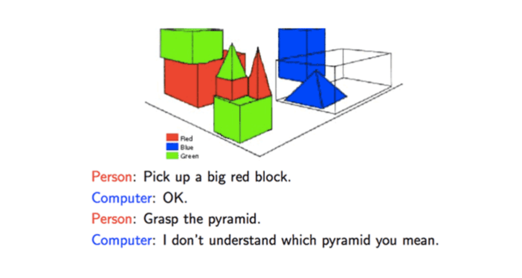
SHRDLU, operating in a block world, aimed to understand and execute natural language instructions for manipulating virtual objects made of various shaped blocks.
[Source: Cryptlabs]
1980s: In the 1980s, code generators, such as The Last One, emerged as tools that could automatically generate code based on user specifications or predefined templates. While not strictly AI-powered in the modern sense, they laid the foundation for later advancements in code generation and automation.
“Personal Computer” magazine cover from 1982 that explored the program, The Last One.
[Source: David Tebbutts]
1990s: Neural network–based predictive models were increasingly applied to code-related tasks, such as predicting program behavior, detecting software defects, and analyzing code quality. These models leveraged the pattern recognition capabilities of neural networks to learn from code examples and make predictions.
2000s: Refactoring tools with AI capabilities began to emerge in the 2000s, offering automated assistance for restructuring and improving code without changing its external behavior. These tools used AI techniques to analyze code patterns, identify opportunities for refactoring, and suggest appropriate refactorings to developers.
These early AI-powered coding tools helped shape the evolution of software development and set the stage for today’s AI-driven coding assistance and automation tools, which continue to evolve seemingly every day.
Evolving beyond the IDE
Initially, AI tools were primarily confined to the integrated development environment (IDE), aiding developers in writing and refining code. But now, we’re starting to see AI touch every part of the software development lifecycle (SDLC), which we’ve found can increase productivity, streamline collaboration, and accelerate innovation for engineering teams.
In a 2023 survey of 500 U.S.-based developers, 70% reported experiencing significant advantages in their work, while over 80% said these tools will foster greater collaboration within their teams. Additionally, our research revealed that developers, on average, complete tasks up to 55% faster when using AI coding tools.
Here’s a quick look at where modern AI-powered coding tools are and some of the technical benefits they provide today:
- Code completion and suggestions. Tools like GitHub Copilot use large language models (LLMs) to analyze code context and generate suggestions to make coding more efficient. Developers can now experience a notable boost in productivity as AI can suggest entire lines of code based on the context and patterns learned from developers’ code repositories, rather than just the code in the editor. Copilot also leverages the vast amount of open-source code available on GitHub to enhance its understanding of various programming languages, frameworks, and libraries, to provide developers with valuable code suggestions.
- Generative AI in your repositories. Developers can use tools like GitHub Copilot Chat to ask questions and gain a deeper understanding of their code base in real time. With AI gathering context of legacy code and processes within your repositories, GitHub Copilot Enterprise can help maintain consistency and best practices across an organization’s codebase when suggesting solutions.
- Natural language processing (NLP). AI has recently made great strides in understanding and generating code from natural language prompts. Think of tools like ChatGPT where developers can describe their intent in plain language, and the AI produces valuable outputs, such as executable code or explanations for that code functionality.
- Enhanced debugging with AI. These tools can analyze code for potential errors, offering possible fixes by leveraging historical data and patterns to identify and address bugs more effectively.
To implement AI tools, developers need technical skills and soft skills
There are two different subsets of skills that can help developers as they begin to incorporate AI tools into their development workflows: technical skills and soft skills. Having both technical chops and people skills is super important for developers when they’re diving into AI projects—they need to know their technical skills to make those AI tools work to their advantage, but they also need to be able to work well with others, solve problems creatively, and understand the big picture to make sure the solutions they come up with actually hit the mark for the folks using them.
Let’s take a look at those technical skills first.
Getting technical
Prompt engineering
Prompt engineering involves crafting well-designed prompts or instructions that guide the behavior of AI models to produce desired outputs or responses. It can be pretty frustrating when AI-powered coding assistants don’t generate a valuable output, but that can often be quickly remedied by adjusting how you communicate with the AI. Here are some things to keep in mind when crafting natural language prompts:
- Be clear and specific. Craft direct and contextually relevant prompts to guide AI models more effectively.
- Experiment and iterate. Try out various prompt variations and iterate based on the outputs you receive.
- Validate, validate, validate. Similar to how you would inspect code written by a colleague, it’s crucial to consistently evaluate, analyze, and verify code generated by AI algorithms.
Code reviews
AI is helpful, but it isn’t perfect. While LLMs are trained on large amounts of data, they don’t inherently understand programming concepts the way humans do. As a result, the code they generate may contain syntax errors, logic flaws, or other issues. That’s why developers need to rely on their coding competence and organizational knowledge to make sure that they aren’t pushing faulty code into production.
For a successful code review, you can start out by asking: does this code change accomplish what it is supposed to do? From there, you can take a look at this in-depth checklist of more things to keep in mind when reviewing AI-generated code suggestions.
Testing and security
With AI’s capabilities, developers can now generate and automate tests with ease, making their testing responsibilities less manual and more strategic. To ensure that the AI-generated tests cover critical functionality, edge cases, and potential vulnerabilities effectively, developers will need a strong foundational knowledge of programming skills, testing principles, and security best practices. This way, they’ll be able to interpret and analyze the generated tests effectively, identify potential limitations or biases in the generated tests, and augment with manual tests as necessary.
Here’s a few steps you can take to assess the quality and reliability of AI-generated tests:
- Verify test assertions. Check if the assertions made by the AI-generated tests are verifiable and if they align with the expected behavior of the software.
- Assess test completeness. Evaluate if the AI-generated tests cover all relevant scenarios and edge cases and identify any gaps or areas where additional testing may be required to achieve full coverage.
- Identify limitations and biases. Consider factors such as data bias, algorithmic biases, and limitations of the AI model used for test generation.
- Evaluate results. Investigate any test failures or anomalies to determine their root causes and implications for the software.
For those beginning their coding journey, check out the GitHub Learning Pathways to gain deeper insights into testing strategies and security best practices with GitHub Actions and GitHub Advanced Security.
You can also bolster your security skills with this new, open source Secure Code Game 🎮.
And now, the soft skills
As developers leverage AI to build what’s next, having soft skills—like the ability to communicate and collaborate well with colleagues—is becoming more important than ever.
Let’s take a more in-depth look at some soft skills that developers can focus on as they continue to adopt AI tools:
- Communication. Communication skills are paramount to collaborating with team members and stakeholders to define project requirements, share insights, and address challenges. They’re also important as developers navigate prompt engineering. The best AI prompts are clear, direct, and well thought out—and communicating with fellow humans in the workplace isn’t much different.
| Did you know that prompt engineering best practices just might help you build your communication skills with colleagues? Check out this thought piece from Harvard Business Review for more insights. |
- Problem solving. Developers may encounter complex challenges or unexpected issues when working with AI tools, and the ability to think creatively and adapt to changing circumstances is crucial for finding innovative solutions.
- Adaptability. The rapid advancement of AI technology requires developers to be adaptable and willing to embrace new tools, methodologies, and frameworks. Plus, cultivating soft skills that promote a growth mindset allows individuals to consistently learn and stay updated as AI tools continue to evolve.
- Ethical thinking. Ethical considerations are important in AI development, particularly regarding issues such as bias, fairness, transparency, and privacy. Integrity and ethical reasoning are essential for making responsible decisions that prioritize the well-being of users and society at large.
- Empathy. Developers are often creating solutions and products for end users, and to create valuable user experiences, developers need to be able to really understand the user’s needs and preferences. While AI can help developers create these solutions faster, through things like code generation or suggestions, developers still need to be able to QA the code and ensure that these solutions still prioritize the well-being of diverse user groups.
Sharpening these soft skills can ultimately augment a developer’s technical expertise, as well as enable them to work more effectively with both their colleagues and AI tools.
Take this with you
As AI continues to evolve, it’s not just changing the landscape of software development; it’s also poised to revolutionize how developers learn and write code. AI isn’t replacing developers—it’s complementing their work, all while providing them with the opportunity to focus more on coding and building their skill sets, both technical and interpersonal.
If you’re interested in improving your skills along your AI-powered coding journey, check out these repositories to start building your own AI based projects. Or you can test out GitHub Copilot, which can help you learn new programming languages, provide coding suggestions, and ask important coding questions right in your terminal.
The post Hard and soft skills for developers coding in the age of AI appeared first on The GitHub Blog.