Post Syndicated from Patrik Nagel original https://aws.amazon.com/blogs/architecture/content-repository-for-unstructured-data-with-multilingual-semantic-search-part-2/
Leveraging vast unstructured data poses challenges, particularly for global businesses needing cross-language data search. In Part 1 of this blog series, we built the architectural foundation for the content repository. The key component of Part 1 was the dynamic access control-based logic with a web UI to upload documents.
In Part 2, we extend the content repository with multilingual semantic search capabilities while maintaining the access control logic from Part 1. This allows users to ingest documents in content repository across multiple languages and then run search queries to get reference to semantically similar documents.
Solution overview
Building on the architectural foundation from Part 1, we introduce four new building blocks to extend the search functionality.
Optical character recognition (OCR) workflow: To automatically identify, understand, and extract text from ingested documents, we use Amazon Textract and a sample review dataset of .png format documents (Figure 1). We use Amazon Textract synchronous application programming interfaces (APIs) to capture key-value pairs for the reviewid and reviewBody attributes. Based on your specific requirements, you can choose to capture either the complete extracted text or parts the text.

Figure 1. Sample document for ingestion
Embedding generation: To capture the semantic relationship between the text, we use a machine learning (ML) model that maps words and sentences to high-dimensional vector embeddings. You can use Amazon SageMaker, a fully-managed ML service, to build, train, and deploy your ML models to production-ready hosted environments. You can also deploy ready-to-use pre-trained models from multiple avenues such as SageMaker JumpStart. For this blog post, we use the open-source pre-trained universal-sentence-encoder-multilingual model from TensorFlow Hub. The model inference endpoint deployed to a SageMaker endpoint generates embeddings for the document text and the search query. Figure 2 is an example of n-dimensional vector that is generated as the output of the reviewBody attribute text provided to the embeddings model.

Figure 2. Sample embedding representation of the value of reviewBody
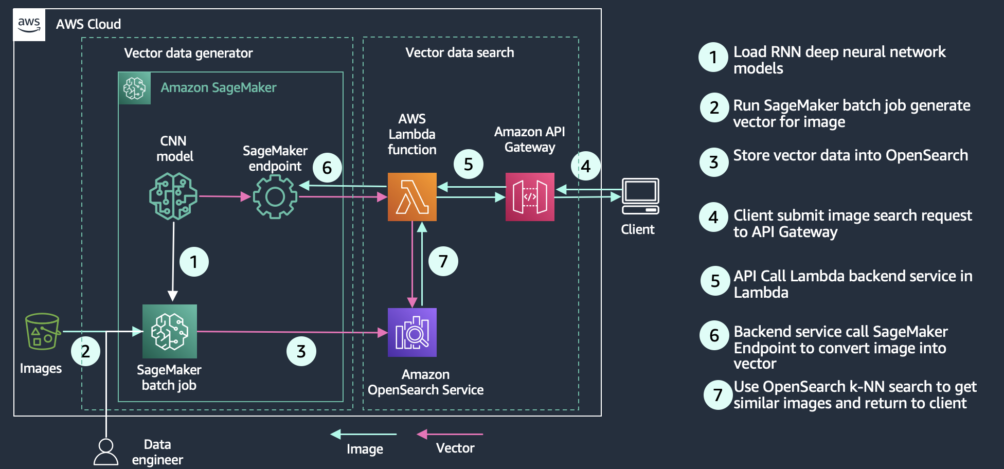
Embedding ingestion: To make the embeddings searchable for the content repository users, you can use the k-Nearest Neighbor (k-NN) search feature of Amazon OpenSearch Service. The OpenSearch k-NN plugin provides different methods. For this blog post, we use the Approximate k-NN search approach, based on the Hierarchical Navigable Small World (HNSW) algorithm. HNSW uses a hierarchical set of proximity graphs in multiple layers to improve performance when searching large datasets to find the “nearest neighbors” for the search query text embeddings.
Semantic search: We make the search service accessible as an additional backend logic on Amazon API Gateway. Authenticated content repository users send their search query using the frontend to receive the matching documents. The solution maintains end-to-end access control logic by using the user’s enriched Amazon Cognito provided identity (ID) token claim with the department attribute to compare it with the ingested documents.
Technical architecture
The technical architecture includes two parts:
- Implementing multilingual semantic search functionality: Describes the processing workflow for the document that the user uploads; makes the document searchable.
- Running input search query: Covers the search workflow for the input query; finds and returns the nearest neighbors of the input text query to the user.
Part 1. Implementing multilingual semantic search functionality
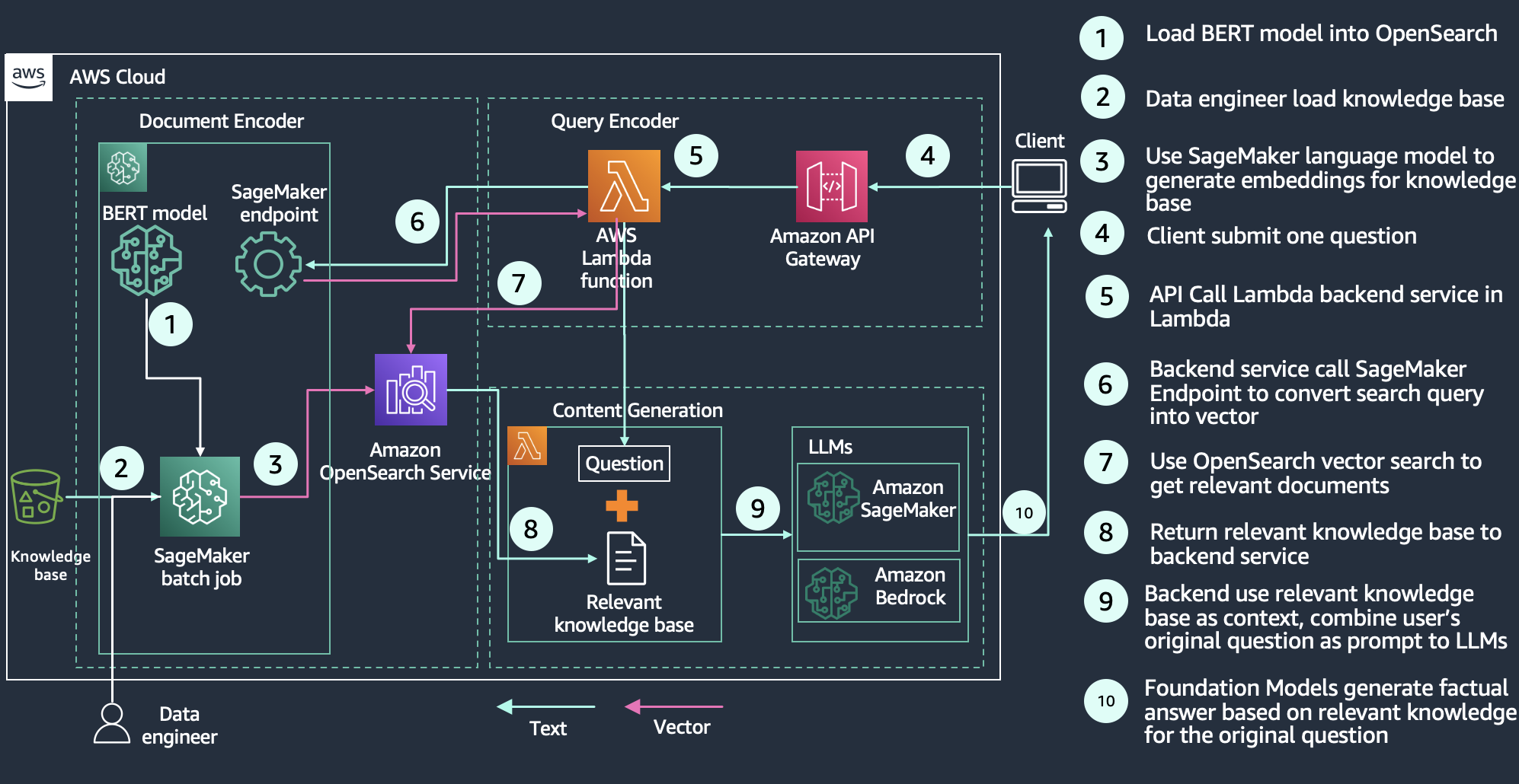
Our previous blog post discussed blocks A through D (Figure 3), including user authentication, ID token enrichment, Amazon Simple Storage Service (Amazon S3) object tags for dynamic access control, and document upload to the source S3 bucket. In the following section, we cover blocks E through H. The overall workflow describes how an unstructured document is ingested in the content repository, run through the backend OCR and embeddings generation process and finally the resulting vector embedding are stored in OpenSearch service.

Figure 3. Technical architecture for implementing multilingual semantic search functionality
- The OCR workflow extracts text from your uploaded documents.
- The source S3 bucket sends an event notification to Amazon Simple Queue Service (Amazon SQS).
- The document transformation AWS Lambda function subscribed to the Amazon SQS queue invokes an Amazon Textract API call to extract the text.
- The document transformation Lambda function makes an inference request to the encoder model hosted on SageMaker. In this example, the Lambda function submits the
reviewBodyattribute to the encoder model to generate the embedding. - The document transformation Lambda function writes an output file in the transformed S3 bucket. The text file consists of:
- The
reviewidandreviewBodyattributes extracted from Step 1 - An additional
reviewBody_embeddingsattribute from Step 2
Note: The workflow tags the output file with the same S3 object tags as the source document for downstream access control.
- The
- The transformed S3 bucket sends an event notification to invoke the indexing Lambda function.
- The indexing Lambda function reads the text file content. Then indexing Lambda function makes an OpenSearch index API call along with source document tag as one of the indexing attributes for access control.
Part 2. Running user-initiated search query
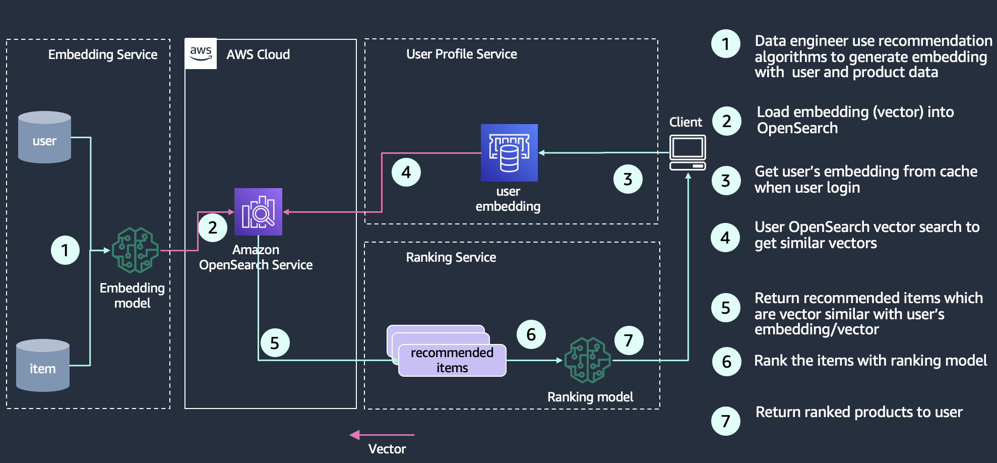
Next, we describe how the user’s request produces query results (Figure 4).

Figure 4. Search query lifecycle
- The user enters a search string in the web UI to retrieve relevant documents.
- Based on the active sign-in session, the UI passes the user’s ID token to the search endpoint of the API Gateway.
- The API Gateway uses Amazon Cognito integration to authorize the search API request.
- Once validated, the search API endpoint request invokes the search document Lambda function.
- The search document function sends the search query string as the inference request to the encoder model to receive the embedding as the inference response.
- The search document function uses the embedding response to build an OpenSearch k-NN search query. The HNSW algorithm is configured with the Lucene engine and its filter option to maintain the access control logic based on the custom
departmentclaim from the user’s ID token. The OpenSearch query returns the following to the query embeddings:- Top three Approximate k-NN
- Other attributes, such as
reviewidandreviewBody
- The workflow sends the relevant query result attributes back to the UI.
Prerequisites
You must have the following prerequisites for this solution:
- An AWS account. Sign up to create and activate one.
- The following software installed on your development machine, or use an AWS Cloud9 environment:
- AWS Command Line Interface (AWS CLI); configure it to point to your AWS account
- TypeScript; use a package manager, such as npm
- AWS Cloud Development Kit (AWS CDK)
- Docker; ensure it’s running
- Appropriate AWS credentials for interacting with resources in your AWS account.
Walkthrough
Setup
The following steps deploy two AWS CDK stacks into your AWS account:
- content-repo-search-stack (
blog-content-repo-search-stack.ts) creates the environment detailed in Figure 3, except for the SageMaker endpoint, which you create in a spearate step. - demo-data-stack (
userpool-demo-data-stack.ts) deploys sample users, groups, and role mappings.
To continue setup, use the following commands:
- Clone the project Git repository:
git clone https://github.com/aws-samples/content-repository-with-multilingual-search content-repository - Install the necessary dependencies:
cd content-repository/backend-cdk npm install - Configure environment variables:
export CDK_DEFAULT_ACCOUNT=$(aws sts get-caller-identity --query 'Account' --output text) export CDK_DEFAULT_REGION=$(aws configure get region) - Bootstrap your account for AWS CDK usage:
cdk bootstrap aws://$CDK_DEFAULT_ACCOUNT/$CDK_DEFAULT_REGION - Deploy the code to your AWS account:
cdk deploy --all
The complete stack set-up may take up to 20 minutes.
Creation of SageMaker endpoint
Follow below steps to create the SageMaker endpoint in the same AWS Region where you deployed the AWS CDK stack.
-
- Sign in to the SageMaker console.
- In the navigation menu, select Notebook, then Notebook instances.
- Choose Create notebook instance.
- Under the Notebook instance settings, enter
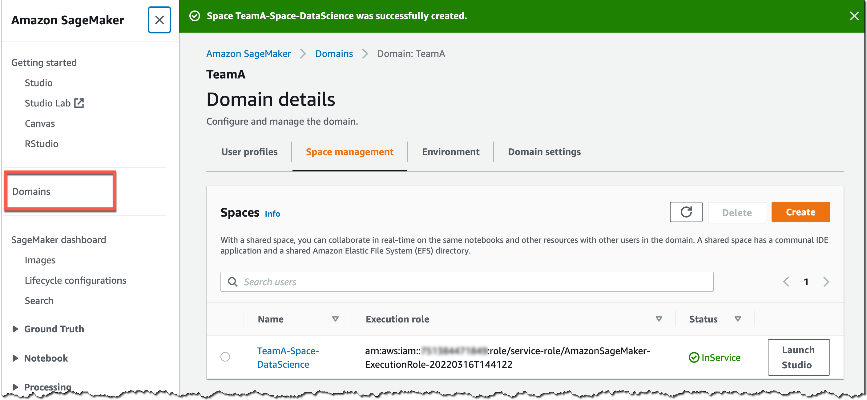
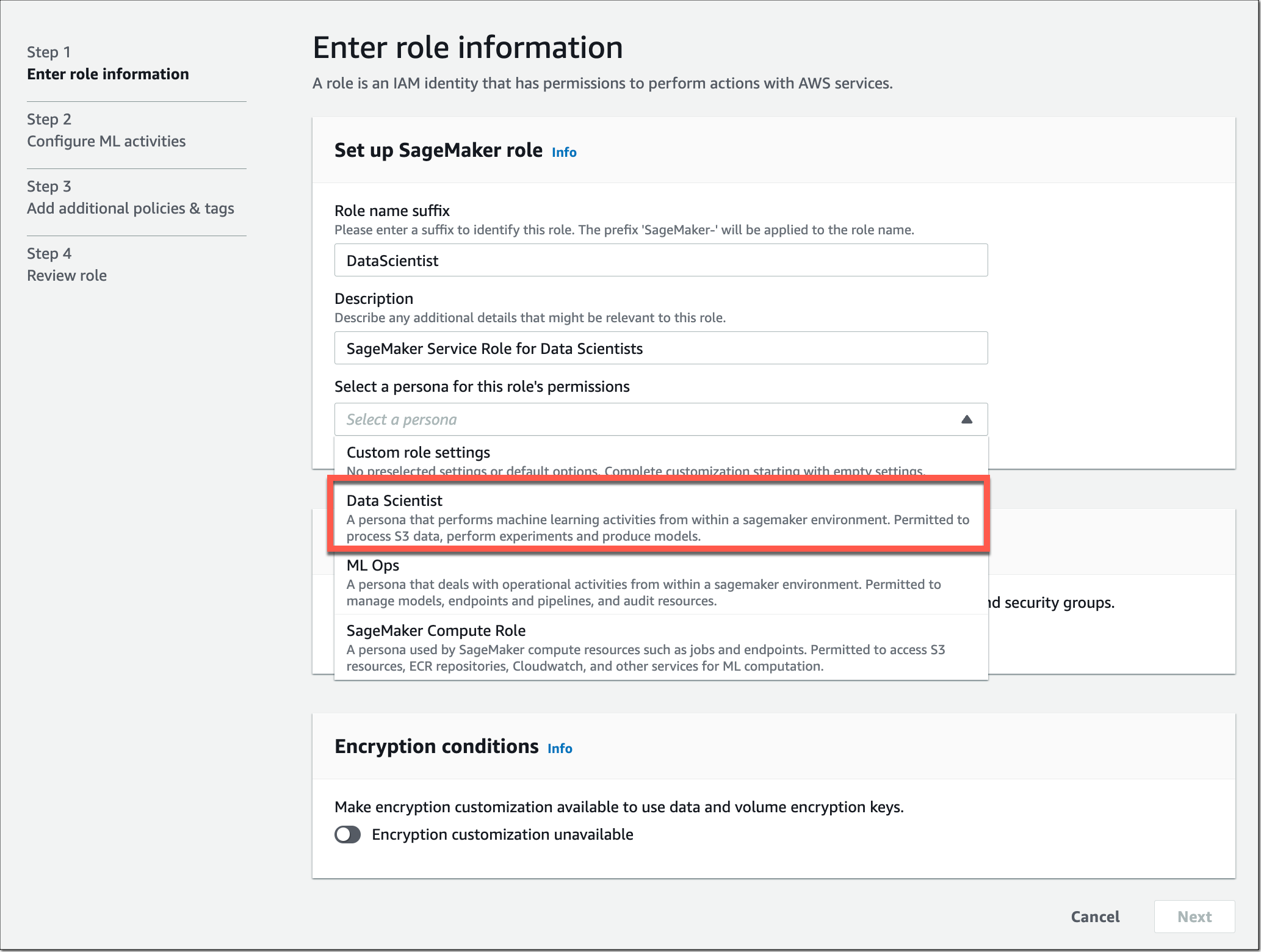
content-repo-notebookas the notebook instance name, and leave other defaults as-is. - Under the Permissions and encryption section (Figure 5), you need to set the IAM role section to the role with the prefix
content-repo-search-stack. In case you don’t see this role automatically populated, select it from the drop-down. Leave the rest of the defaults, and choose Create notebook instance.
Figure 5. Notebook permissions
- The notebook creation status changes to
Pendingbefore it’s available for use within 3-4 minutes. - Once the notebook is in the
Availablestatus, choose Open Jupyter. - Choose the Upload button and upload the
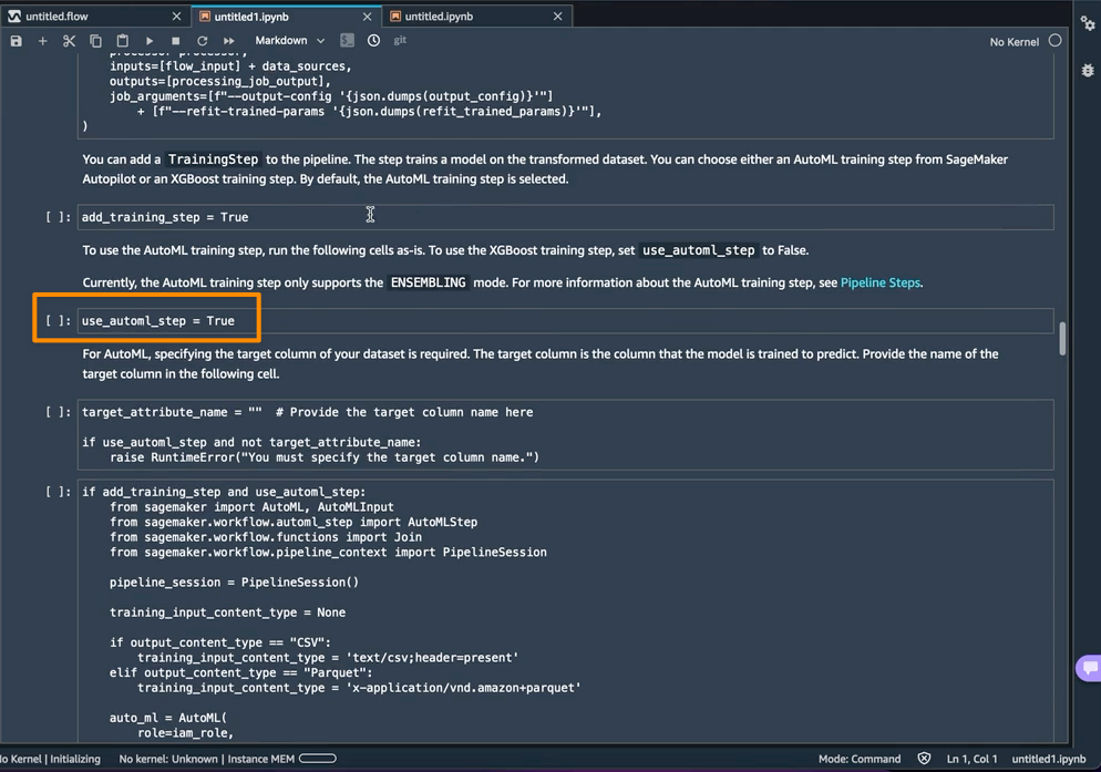
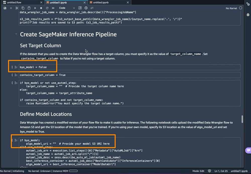
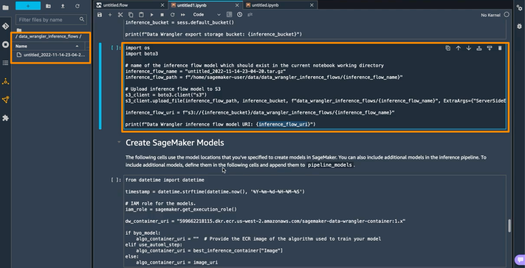
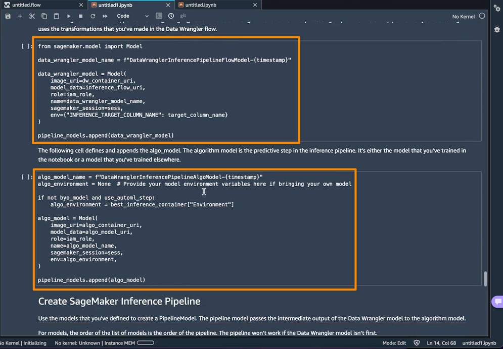
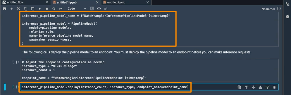
create-sagemaker-endpoint.ipynbfile in thebackend-cdkfolder of the root of the blog repository. - Open the
create-sagemaker-endpoint.ipynbnotebook. Select the option Run All from the Cell menu (Figure 6). This might take up to 10 minutes.
Figure 6. Run
create-sagemaker-endpointnotebook cells - After all the cells have successfully run, verify that the AWS Systems Manager parameter
sagemaker-endpointis updated with the value of the SageMaker endpoint name. An example of value as the output of the cell is in Figure 7. In case you don’t see the output, check if the preceding steps were run correctly.
Figure 7. SSM parameter updated with SageMaker endpoint
- Verify in the SageMaker console that the inference endpoint with the prefix
tensorflow-inferencehas been deployed and is set to statusInService. - Upload sample data to the content repository:
- Update the
S3_BUCKET_NAMEvariable in theupload_documents_to_S3.shscript in the root folder of the blog repository with thes3SourceBucketNamefrom the AWS CDK output of the content-repo-search-stack. - Run
upload_documents_to_S3.sh scriptto upload 150 sample documents to the content repository. This takes 5-6 minutes. During this process, the uploaded document triggers the workflow described in the Implementing multilingual semantic search functionality.
- Update the


Using the search service
At this stage, you have deployed all the building blocks for the content repository in your AWS account. Next, as part of the upload sample data to the content repository, you pushed a limited corpus of 150 sample documents (.png format). Each document is in one of the four different languages – English, German, Spanish and French. With the added multilingual search capability, you can query in one language and receive semantically similar results across different languages while maintaining the access control logic.
- Access the frontend application:
- Copy the
amplifyHostedAppUrlvalue of the AWS CDK output from the content-repo-search-stack shown in the terminal. - Enter the URL in your web browser to access the frontend application.
- A temporary page displays until the automated build and deployment of the React application completes after 4-5 minutes.
- Copy the
- Sign into the application:
- The content repository provides two demo users with credentials as part of the demo-data-stack in the AWS CDK output. Copy the password from the terminal associated with the
sales-user, which belongs to thesalesdepartment. - Follow the prompts from the React webpage to sign in with the sales-user and change the temporary password.
- The content repository provides two demo users with credentials as part of the demo-data-stack in the AWS CDK output. Copy the password from the terminal associated with the
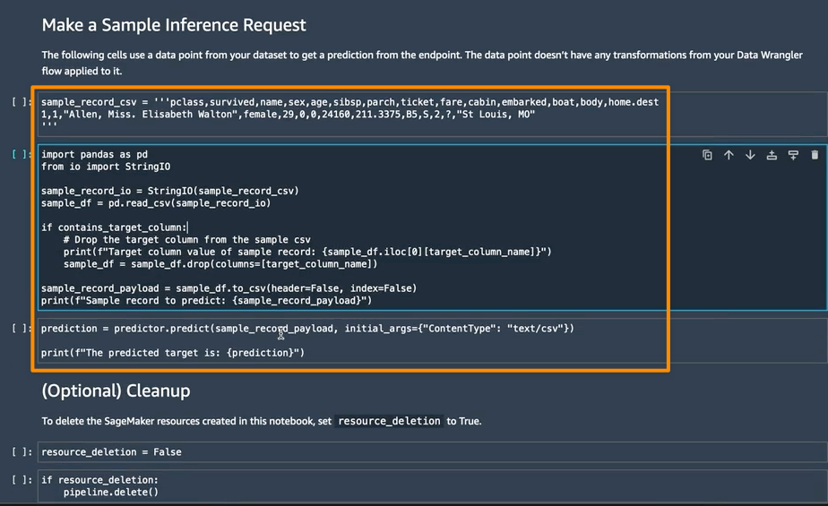
- Enter search queries and verify results. The search action invokes the workflow described in Running input search query. For example:
- Enter
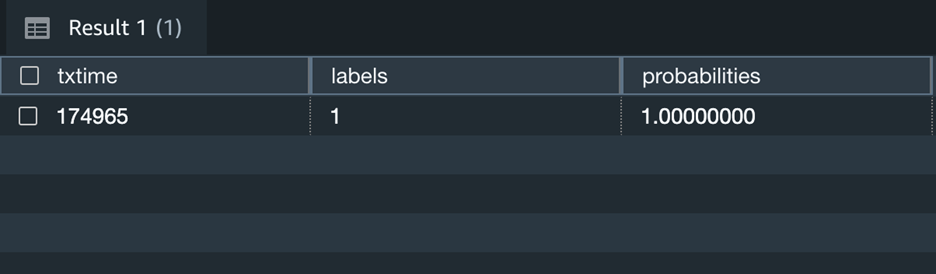
works wellas the search query. Note the multilingual output and the semantically similar results (Figure 8).
-
Figure 8. Positive sentiment multilingual search result for the sales-user
- Enter
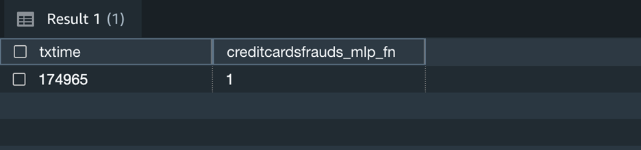
bad qualityas the search query. Note the multilingual output and the semantically similar results (Figure 9).
Figure 9. Negative sentiment multi-lingual search result for the sales-user
- Enter
- Sign out as the
sales-userwith the Log Out button on the webpage. - Sign in using the
marketing-usercredentials to verify access control:- Follow the sign in procedure in step 2 but with the
marketing-user. - This time with
works wellas search query, you find different output. This is because the access control only allowsmarketing-userto search for the documents that belong to themarketingdepartment (Figure 10).
Figure 10. Positive sentiment multilingual search result for the marketing-user
- Follow the sign in procedure in step 2 but with the


Cleanup
In the backend-cdk subdirectory of the cloned repository, delete the deployed resources: cdk destroy --all.
Additionally, you need to access the Amazon SageMaker console to delete the SageMaker endpoint and notebook instance created as part of the Walkthrough setup section.
Conclusion
In this blog, we enriched the content repository with multi-lingual semantic search features while maintaining the access control fundamentals that we implemented in Part 1. The building blocks of the semantic search for unstructured documents—Amazon Textract, Amazon SageMaker, and Amazon OpenSearch Service—set a foundation for you to customize and enhance the search capabilities for your specific use case. For example, you can leverage the fast developments in Large Language Models (LLM) to enhance the semantic search experience. You can replace the encoder model with an LLM capable of generating multilingual embeddings while still maintaining the OpenSearch service to store and index data and perform vector search.

 AWS Global Summits – Check your calendars and sign up for the AWS Summit close to where you live or work:


 Nishchai JM is an Analytics Specialist Solutions Architect at Amazon Web services. He specializes in building Big-data applications and help customer to modernize their applications on Cloud. He thinks Data is new oil and spends most of his time in deriving insights out of the Data.
 Varad Ram is Senior Solutions Architect in Amazon Web Services. He likes to help customers adopt to cloud technologies and is particularly interested in artificial intelligence. He believes deep learning will power future technology growth. In his spare time, he like to be outdoor with his daughter and son.
 Narendra Gupta is a Specialist Solutions Architect at AWS, helping customers on their cloud journey with a focus on AWS analytics services. Outside of work, Narendra enjoys learning new technologies, watching movies, and visiting new places
 Arun A K is a Big Data Solutions Architect with AWS. He works with customers to provide architectural guidance for running analytics solutions on the cloud. In his free time, Arun loves to enjoy quality time with his family
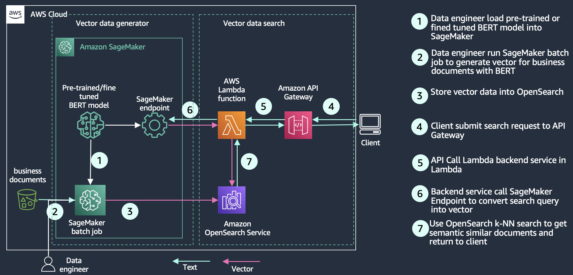
 Jon Handler is a Senior Principal Solutions Architect at Amazon Web Services based in Palo Alto, CA. Jon works closely with OpenSearch and Amazon OpenSearch Service, providing help and guidance to a broad range of customers who have search and log analytics workloads that they want to move to the AWS Cloud. Prior to joining AWS, Jon’s career as a software developer included four years of coding a large-scale, eCommerce search engine. Jon holds a Bachelor of the Arts from the University of Pennsylvania, and a Master of Science and a Ph. D. in Computer Science and Artificial Intelligence from Northwestern University.
 Jianwei Li is a Principal Analytics Specialist TAM at Amazon Web Services. Jianwei provides consultant service for customers to help customer design and build modern data platform. Jianwei has been working in big data domain as software developer, consultant and tech leader.
 Dylan Tong is a Senior Product Manager at AWS. He works with customers to help drive their success on the AWS platform through thought leadership and guidance on designing well architected solutions. He has spent most of his career building on his expertise in data management and analytics by working for leaders and innovators in the space.
 Vamshi Vijay Nakkirtha is a Software Engineering Manager working on the OpenSearch Project and Amazon OpenSearch Service. His primary interests include distributed systems. He is an active contributor to various plugins, like k-NN, GeoSpatial, and dashboard-maps.
 During the preview, we had lots of interest and great feedback from customers. Today, Amazon SageMaker geospatial capabilities are generally available with new security updates and additional sample use cases.
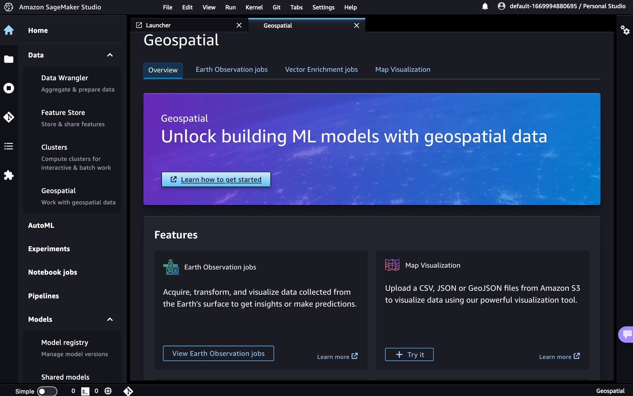


 Kachi Odoemene is an Applied Scientist at AWS AI. He builds AI/ML solutions to solve business problems for AWS customers.
 Taylor McNally is a Deep Learning Architect at Amazon Machine Learning Solutions Lab. He helps customers from various industries build solutions leveraging AI/ML on AWS. He enjoys a good cup of coffee, the outdoors, and time with his family and energetic dog.
 Austin Welch is a Data Scientist in the Amazon ML Solutions Lab. He develops custom deep learning models to help AWS public sector customers accelerate their AI and cloud adoption. In his spare time, he enjoys reading, traveling, and jiu-jitsu.


 AWS and Hugging Face collaborate to make generative AI more accessible and cost-efficient – This previous week, we announced an expanded collaboration between AWS and
 AWS Pi Day – Join me on March 14 for the third annual


 You use map apps every day to find your favorite restaurant or travel the fastest route using geospatial data. There are two types of geospatial data: vector data that uses two-dimensional geometries such as a building location (points), roads (lines), or land boundary (polygons), and raster data such as satellite and aerial images.


