Tag Archives: Amazon Sagemaker

Introducing the next generation of Amazon SageMaker: The center for all your data, analytics, and AI

2024-12-03 Antje Barth

Post Syndicated from Antje Barth original https://aws.amazon.com/blogs/aws/introducing-the-next-generation-of-amazon-sagemaker-the-center-for-all-your-data-analytics-and-ai/

Today, we’re announcing the next generation of Amazon SageMaker, a unified platform for data, analytics, and AI. The all-new SageMaker includes virtually all of the components you need for data exploration, preparation and integration, big data processing, fast SQL analytics, machine learning (ML) model development and training, and generative AI application development.

The current Amazon SageMaker has been renamed to Amazon SageMaker AI. SageMaker AI is integrated within the next generation of SageMaker while also being available as a standalone service for those who wish to focus specifically on building, training, and deploying AI and ML models at scale.

Highlights of the new Amazon SageMaker
At its core is SageMaker Unified Studio (preview), a single data and AI development environment. It brings together functionality and tools from the range of standalone “studios,” query editors, and visual tools that we have today in Amazon Athena, Amazon EMR, AWS Glue, Amazon Redshift, Amazon Managed Workflows for Apache Airflow (MWAA), and the existing SageMaker Studio. We’ve also integrated Amazon Bedrock IDE (preview), an updated version of Amazon Bedrock Studio, to build and customize generative AI applications. In addition, Amazon Q provides AI assistance throughout your workflows in SageMaker.

Here’s a list of key capabilities:

Amazon SageMaker Unified Studio (preview) – Build with all your data and tools for analytics and AI in a single environment.
Amazon SageMaker Lakehouse – Unify data across Amazon Simple Storage Service (Amazon S3) data lakes, Amazon Redshift data warehouses, and third-party and federated data sources with Amazon SageMaker Lakehouse.
Data and AI Governance – Securely discover, govern, and collaborate on data and AI with Amazon SageMaker Catalog, built on Amazon DataZone.
Data Processing – Analyze, prepare, and integrate data for analytics and AI using open source frameworks on Amazon Athena, Amazon EMR, and AWS Glue.
Model development – Build, train, and deploy ML and foundation models (FMs) with fully managed infrastructure, tools, and workflows with Amazon SageMaker AI.
Generative AI app development – Build and scale generative AI applications with Amazon Bedrock.
SQL analytics – Gain insights with Amazon Redshift, the most price-performant SQL engine.

In this post, I give you a quick tour of the new SageMaker Unified Studio experience and how to get started with data processing, model development, and generative AI app development.

Working with Amazon SageMaker Unified Studio (preview)
With SageMaker Unified Studio, you can discover your data and put it to work using familiar AWS tools to complete end-to-end development workflows, including data analysis, data processing, model training, and generative AI app building, in a single governed environment.

An integrated SQL editor lets you query data from multiple sources, and a visual extract, transform, and load (ETL) tool simplifies the creation of data integration and transformation workflows. New unified Jupyter notebooks enable seamless work across different compute services and clusters. With the new built-in data catalog functionality, you can find, access, and query data and AI assets across your organization. Amazon Q is integrated to streamline tasks across the development lifecycle.

Let’s explore the individual capabilities in more detail.

Data processing
SageMaker integrates with SageMaker Lakehouse and lets you analyze, prepare, integrate, and orchestrate your data in a unified experience. You can integrate and process data from various sources using the provided connectivity options.

Start by creating a project in SageMaker Unified Studio, choosing the SQL analytics or data analytics and AI-ML model development project profile. Projects are a place to collaborate with your colleagues, share data, and use tools to work with data in a secure way. Project profiles in SageMaker define the preconfigured set of resources and tools that are provisioned when you create a new project. In your project, choose Data in the left menu and start adding data sources.

The built-in SQL query editor lets you query your data stored in data lakes, data warehouses, databases, and applications directly within SageMaker Unified Studio. In the top menu of SageMaker Unified Studio, select Build and choose Query Editor to get started. Also, try creating SQL queries using natural language with Amazon Q while you’re at it.

You should also explore the built-in visual ETL tool to create data integration and transformation workflows using a visual, drag-and-drop interface. In the top menu, select Build and choose Visual ETL flow to get started.

If Amazon Q is enabled, you can also use generative AI to author flows. Visual ETL comes with a wide range of data connectors, pre-built transformations, and features such as scheduling, monitoring, and data previewing to streamline your data workflows.

Model development
SageMaker Unified Studio includes capabilities from SageMaker AI, which provides infrastructure, tools, and workflows for the entire ML lifecycle. From the top menu, select Build to access tools for data preparation, model training, experiment tracking, pipeline creation, and orchestration. You can also use these tools for model deployment and inference, machine learning operations (MLOps) implementation, model monitoring and evaluation, as well as governance and compliance.

To start your model development, create a project in SageMaker Unified Studio using the data analytics and AI-ML model development project profile and explore the new unified Jupyter notebooks. In the top menu, select Build and choose JupyterLab. You can use the new unified notebooks to seamlessly work across different compute services and clusters. You can use these notebooks to switch between environments without leaving your workspace, streamlining your model development process.

You can also use Amazon Q Developer to assist with tasks such as code generation, debugging, and optimization throughout your model development process.

Generative AI app development
Use the new Amazon Bedrock IDE to develop generative AI applications within Amazon SageMaker Unified Studio. The Amazon Bedrock IDE includes tools to build and customize generative AI applications using FMs and advanced capabilities such as Amazon Bedrock Knowledge Bases, Amazon Bedrock Guardrails, Amazon Bedrock Agents, and Amazon Bedrock Flows to create tailored solutions aligned with your requirements and responsible AI guidelines.

Choose Discover in the top menu of SageMaker Unified Studio to browse Amazon Bedrock models or experiment with the model playgrounds.

Create a project using the GenAI Application Development profile to start building generative AI applications. Choose Build in the top menu of SageMaker Unified Studio and select Chat agent.

With the Amazon Bedrock IDE, you can build chat agents and create knowledge bases from your proprietary data sources with just a few clicks, enabling Retrieval-Augmented Generation (RAG). You can add guardrails to promote safe AI interactions and create functions to integrate with any system. With built-in model evaluation features, you can test and optimize your AI applications’ performance while collaborating with your team. Design flows for deterministic genAI-powered workflows, and when ready, share your applications or prompts within the domain or export them for deployment anywhere—all while maintaining control of your project and domain assets.

For a detailed description of all Amazon SageMaker capabilities, check the SageMaker Unified Studio User Guide.

Getting started
To begin using SageMaker Unified Studio, administrators need to complete several setup steps. This includes setting up AWS IAM Identity Center, configuring the necessary virtual private cloud (VPC) and AWS Identity and Access Management (IAM) roles, creating a SageMaker domain, and enabling Amazon Q Developer Pro. Instead of IAM Identity Center, you can also configure SAML through IAM federation for user management.

After the environment is configured, users sign in through the provided SageMaker Unified Studio domain URL with single sign-on. You can create projects to collaborate with team members, choosing from pre-configured project profiles for different use cases. Each project connects to a Git repository for version control and includes an example unified Jupyter notebook to get you started.

For detailed setup instructions, check the SageMaker Unified Studio Administrator Guide.

Now available
The next generation of Amazon SageMaker is available today in the US East (N. Virginia, Ohio), US West (Oregon), Asia Paciﬁc (Tokyo), and Europe (Ireland) AWS Regions. Amazon SageMaker Uniﬁed Studio and Amazon Bedrock IDE are available today in preview in these AWS Regions. Check the full Region list for future updates.

For pricing information, visit Amazon SageMaker pricing and Amazon Bedrock pricing. To learn more, visit Amazon SageMaker, SageMaker Unified Studio, and Amazon Bedrock IDE.

Existing Amazon Bedrock Studio preview domains will be available until February 28, 2025, but you may not create new workspaces. To experience the advanced features of Bedrock IDE, create a new SageMaker domain following the instructions in the Administrator Guide.

Give the new Amazon SageMaker a try in the console today and let us know what you think! Send feedback to AWS re:Post for Amazon SageMaker or through your usual AWS Support contacts.

— Antje

Manage access controls in generative AI-powered search applications using Amazon OpenSearch Service and Amazon Cognito

2024-11-19 Karim Akhnoukh

Post Syndicated from Karim Akhnoukh original https://aws.amazon.com/blogs/big-data/manage-access-controls-in-generative-ai-powered-search-applications-using-amazon-opensearch-service-and-aws-cognito/

Organizations of all sizes and types are using generative AI to create products and solutions. A common adoption pattern is to introduce document search tools to internal teams, especially advanced document searches based on semantic search. In semantic search, documents are stored as vectors, a numeric representation of the document content, in a vector database such as Amazon OpenSearch Service, and are retrieved by performing similarity search with a vector representation of the search query.

In a real-world scenario, organizations want to make sure their users access only documents they are entitled to access. They are looking for a reliable and scalable solution to implement robust access controls to make sure these documents are only accessible to individuals who have a legitimate business need and the appropriate level of authorization. The permission mechanism has to be secure, built on top of built-in security features, and scalable for manageability when the user base scales out. Maintaining proper access controls for these sensitive assets is paramount, because unauthorized access could lead to severe consequences, such as data breaches, compliance violations, and reputational damage.

In this post, we show you how to manage user access to enterprise documents in generative AI-powered tools according to the access you assign to each persona.

Common use cases

The following are industry-specific use cases for document access management across different departments:

In R&D and engineering, access to product design documents evolves from restricted to broader as development progresses
HR maintains open access to general policies while limiting access to sensitive employee information
Finance and accounting documents require varying levels of access for auditing and executive decision-making
Sales and marketing teams carefully manage customer data and strategies, implementing tiered access for different roles and departments

These examples demonstrate the need for dynamic, role-based access control to balance information sharing with confidentiality in various business contexts.

Solution overview

By combining the powerful vector search capabilities of OpenSearch Service with the access control features provided by Amazon Cognito, this solution enables organizations to manage access controls based on custom user attributes and document metadata.

This approach simplifies the management of access rights, making sure only authorized users can access and interact with specific documents based on their roles, departments, and other relevant attributes. Following this approach, you can manage the access to your organization’s documents at scale. The following diagram depicts the solution architecture.

The solution workflow consists of the following steps:

The user accesses a smart search portal and lands on a web interface deployed on AWS Amplify.
The user authenticates through an Amazon Cognito user pool and an access token is returned to the client. This access token will be used to retrieve the key pair custom attributes assigned to the user. In our case, we created two custom attributes (custom:department and custom:access_level).
For each user query, an API is invoked on Amazon API Gateway to process the request. Each invocation includes the user access token in the header.
The API is integrated with AWS Lambda, which processes the user query and generates the answers based on available documents and user access using retrieval augmented generation (RAG). The process starts by creating a vector based on the question (embedding) by invoking the embedding model.
A query is sent to OpenSearch Service that includes the following:
1. The embedding vector generated.
2. User custom attributes retrieved by Lambda based on their access token, by calling the Amazon Cognito GetUser API.
3. The query relies on the support of an efficient k-NN filter in OpenSearch Service to perform the search.
Pre-filtered documents that relate to the user query are included in the prompt of the large language model (LLM) that summarizes the answer. Then, Lambda replies back to the web interface with the LLM completion (reply).
If the user’s access needs to be modified (assigned attributes), an API call is made through API Gateway to a Lambda function that processes the request to add or update the custom attributes’ value for a specific user.
New attributes are reflected in the user’s profile in Amazon Cognito.

Our solution is implemented and wrapped within AWS Cloud Development Kit (AWS CDK) stacks, which are available in the GitHub repo.

Our sample documents assume a fictional manufacturing company called Unicorn Robotics Factory, which develops robotic unicorns. The dataset contains over 900 documents that are a mix of engineering, roadmap, and business reporting documents. The following is an example of a document’s content:

**CONFIDENTIAL - UNICORNS ROBOTICS INTERNAL DOCUMENT**

**Project: "Galactic Unicorn"**

Unicorns Robotics is proud to announce the development of our latest project, the "Galactic Unicorn". 
This top-secret project aims to create a robotic unicorn that can travel through space and time, bringing magic and joy to children and adults alike.....

The associated metadata file for this document consists of the following:

{ "department": "research", "access_level": "confidential" }

Our solution in the GitHub repo takes care of loading the documents with associated metadata tags. For illustration purposes, we used the following mapping for the users and document access.

This solution is meant to delegate access management to the application tier, to simplify the implementation of use cases like generative AI-powered document search tools. However, if your use case requires a stricter approach to control document access, like multi-tenant environments or field-level security, you might want to use the fine-grained access control feature in OpenSearch Service. In our solution, we manage the access on the document level according to the assigned metadata.

Prerequisites

To deploy the solution, you need the following prerequisites:

An AWS account. If you don’t already have an AWS account, you can create one.
Your access to the AWS account must have AWS Identity and Access Management (IAM) permissions to launch AWS CloudFormation templates that create IAM roles.
The AWS Command Line Interface (AWS CLI) installed.
node.js and npm installed for the frontend.
Docker installed.
The AWS CDK configured. For more information, see Getting started with the AWS CDK.
In case of LLM inference based on Amazon SageMaker, a sufficient service limit to deploy an ml.g5.12xlarge instance for the SageMaker endpoint. If needed, you can initiate a quota increase request. Refer to Service Quotas for more details.

Deploy the solution

To deploy the solution to your AWS account, refer to the Readme file in our GitHub repo.

Query documents with different personas

Now let’s test the application using different personas. In this example, we use the same users with their corresponding custom attributes as illustrated in the solution overview.

To start, let’s log in using the researcher account and run the search around a confidential document.

We ask, “What is the projected profit margin of the Galactic Unicorn project?” and get the result as shown in the following screenshot.

The question invokes a query to OpenSearch Service using the custom attributes assigned to the researcher. The following code illustrates how the query is structured:

for attr, values in user_attributes.items():
        must_conditions.append(
            {
                "bool": {
                    "should": [{"term": {attr: value}} for value in values],
                    "minimum_should_match": 1,
                }
            }
        )

query = {
        "size": 5,
        "query": {
            "knn": {
                "doc_embedding": {
                    "vector": query_vector,
                    "k": 10,
                    "filter": {"bool": {"must": must_conditions}},
                }
            }
        },
    }

Let’s sign out and log in again with an engineer profile to test the same query. Based on the assigned attributes and document metadata, the result should look like that in the following screenshot.

If you tried to query some support documents, you will get the desired answer, as shown in the following screenshot.

Modify user access

As depicted in the solution diagram, we’ve added a feature in the web interface to allow you to modify user access, which you could use to perform further tests. To do so, log in as a tool admin and choose Manage Attributes. Then modify the custom attribute value for a given user, as shown in the following screenshot.

Clean up

When deleting a stack, most resources will be deleted upon stack deletion, but that’s not the case for all resources. The Amazon Simple Storage Service (Amazon S3) bucket, Amazon Cognito user pool, and OpenSearch Service domain will be retained by default. However, our AWS CDK code altered this default behavior by setting the RemovalPolicy to DESTROY for the mentioned resources. If you want to retain them, you can adjust the RemovalPolicy in the AWS CDK code for the different resources.

You can use the following command to clean up the resources deployed to your AWS account:

make destroy

Conclusion

This post illustrated how to build a document search RAG solution that makes sure only authorized users can access and interact with specific documents based on their roles, departments, and other relevant attributes. It combines OpenSearch Service and Amazon Cognito custom attributes to make a tag-based access control mechanism that makes it straightforward to manage at scale.

For demonstration purposes, the following points weren’t included in the AWS CDK code. However, they’re still applicable and you might want to work on them before deploying for production purposes:

OpenSearch Service best practices, such as instance sizing and using primary nodes
Advanced document chunking strategies for RAG implementations, such as recursive or semantic chunking

About the Authors

Karim Akhnoukh is a Solutions Architect at AWS working with manufacturing customers in Germany. He is passionate about applying machine learning and generative AI to solve customers’ business challenges. Besides work, he enjoys playing sports, aimless walks, and good quality coffee.

Ahmed Ewis is a Senior Solutions Architect at AWS GenAI Labs. He helps customers build generative AI-based solutions to solve business problems. When not collaborating with customers, he enjoys playing with his kids and cooking.

Fortune Hui is a Solutions Architect at AWS Hong Kong, working with conglomerate customers. He helps customers and partners build big data platform and generative AI applications. In his free time, he plays badminton and enjoys whisky.

AWS Weekly Roundup: Jamba 1.5 family, Llama 3.2, Amazon EC2 C8g and M8g instances and more (Sep 30, 2024)

2024-09-30 Elizabeth Fuentes

Post Syndicated from Elizabeth Fuentes original https://aws.amazon.com/blogs/aws/aws-weekly-roundup-jamba-1-5-family-llama-3-2-amazon-ec2-c8g-and-m8g-instances-and-more-sep-30-2024/

Every week, there’s a new Amazon Web Services (AWS) community event where you can network, learn something new, and immerse yourself in the community. When you’re in a community, everyone grows together, and no one is left behind. Last week was no exception. I can highlight the Dutch AWS Community Day where Viktoria Semaan closed with a talk titled How to Create Impactful Content and Build a Strong Personal Brand, and the Peru User Group, who organized two days of talks and learning opportunities: UGCONF & SERVERLESSDAY 2024, featuring Jeff Barr, who spoke about how to Create Your Own Luck. The community events continue, so check them out at Upcoming AWS Community Days.

Last week’s launches
Here are the launches that got my attention.

Jamba 1.5 family of models by AI21 Labs is now available in Amazon Bedrock – The Jamba 1.5 Large and 1.5 Mini models feature a 256k context window, one of the longest on the market, enabling complex tasks like lengthy document analysis. With native support for structured JSON output, function calling, and document processing, they integrate into enterprise workflows for specialized AI solutions. To learn more, read Jamba 1.5 family of models by AI21 Labs is now available in Amazon Bedrock, visit the AI21 Labs in Amazon Bedrock page, and read the documentation.

AWS Lambda now supports Amazon Linux 2023 runtimes in AWS GovCloud (US) Regions – These runtimes offer the latest language features, including Python 3.12, Node.js 20, Java 21, .NET 8, Ruby 3.3, and Amazon Linux 2023. They have smaller deployment footprints, updated libraries, and a new package manager. Additionally, you can also use the container base images to build and deploy functions as a container image.

Amazon SageMaker Studio now supports automatic shutdown of idle applications – You can now enable automatic shutdown of inactive JupyterLab and CodeEditor applications using Amazon SageMaker Distribution image v2.0 or newer. Administrators can set idle shutdown times at domain or user profile levels, with optional user customization. This cost control mechanism helps avoid charges for unused instances and is available across all AWS Regions where SageMaker Studio is offered.

Amazon S3 is implementing a default 128 KB minimum object size for S3 Lifecycle transition rules to any S3 storage class – Reduce transition costs for datasets with many small objects by decreasing transition requests. Users can override the default and customize minimum object sizes. Existing rules remain unchanged, but the new default applies to new or modified configurations.

AWS Lake Formation centralized access control for Amazon Redshift data sharing is now available in 11 additional Regions – Enabling granular permissions management, including table, column, and row-level access to shared Amazon Redshift data. It also supports tag-based access control and trusted identity propagation with AWS IAM Identity Center for improved security and simplified management.

Llama 3.2 generative AI models now available in Amazon Bedrock – The collection includes 90B and 11B parameter multimodal models for sophisticated reasoning tasks, and 3B and 1B text-only models for edge devices. These models support vision tasks, offer improved performance, and are designed for responsible AI innovation across various applications. These models support a 128K context length and multilingual capabilities in eight languages. Learn more about it in Introducing Llama 3.2 models from Meta in Amazon Bedrock.

Share AWS End User Messaging SMS resources across multiple AWS accounts – You can use AWS Resource Access Manager (RAM), to share phone numbers, sender IDs, phone pools, and opt-out lists. Additionally, Amazon SNS now delivers SMS text messages through AWS End User Messaging, offering enhanced features like two-way messaging and granular permissions. These updates provide greater flexibility and control for SMS messaging across AWS services.

AWS Serverless Application Repository now supports AWS PrivateLink – Enabling direct connection from Amazon Virtual Private Cloud (VPC) without internet exposure. This enhances security by keeping communication within the AWS network. Available in all Regions where AWS Serverless Application Repository is offered, it can be set up using the AWS Management Console or AWS Command Line Interface (AWS CLI).

Amazon SageMaker with MLflow now supports AWS PrivateLink for secure traffic routing – Enabling secure data transfer from Amazon Virtual Private Cloud (VPC) to MLflow Tracking Servers within the AWS network. This enhances protection of sensitive information by avoiding public internet exposure. Available in most AWS Regions, it improves security for machine learning (ML) and generative AI experimentation using MLflow.

Introducing Amazon EC2 C8g and M8g Instances – Enhanced performance for compute-intensive and general-purpose workloads. With up to three times more vCPUs, three times more memory, 75 percent more memory bandwidth, and two times more L2 cache, these instances improve data processing, scalability, and cost-efficiency for various applications including high performance computing (HPC), batch processing, and microservices. Read more in Run your compute-
intensive and general purpose workloads sustainably with the new Amazon EC2 C8g, M8g instances.

Llama 3.2 models are now available in Amazon SageMaker JumpStart – These models offer various sizes from 1B to 90B parameters, support multimodal tasks, including image reasoning, and are more efficient for AI workloads. The 1B and 3B models can be fine-tuned, while Llama Guard 3 11B Vision supports responsible innovation and system-level safety. Learn more in Llama 3.2 models from Meta are now available in Amazon SageMaker JumpStart.

For a full list of AWS announcements, be sure to keep an eye on the What’s New at AWS page.

Other AWS news
Here are some additional projects, blog posts, and news items that you might find interesting:

Deploy generative AI agents in your contact center for voice and chat using Amazon Connect, Amazon Lex, and Amazon Bedrock Knowledge Bases – This solution enables low-latency customer interactions, answering queries from a knowledge base. Features include conversation analytics, automated testing, and hallucination detection in a serverless architecture.

How AWS WAF threat intelligence features help protect the player experience for betting and gaming customers – AWS WAF enhances bot protection for betting and gaming. New features include browser fingerprinting, automation detection, and ML models to identify coordinated bots. These tools combat scraping, fraud, distributed denial of service (DDoS) attacks, and cheating, safeguarding player experiences.

How to migrate 3DES keys from a FIPS to a non-FIPS AWS CloudHSM cluster – Learn how to securely transfer Triple Data Encryption Algorithm (3DES) keys from Federal Information Processing Standard (FIPS) hsm1 to non-FIPS hsm2 clusters using RSA-AES wrapping, without backups. This enables using new hsm2.medium instances with FIPS 140-3 Level 3 support, non-FIPS mode, increased key capacity, and mutual TLS (mTLS).

Upcoming AWS events
Check your calendars and sign up for upcoming AWS events:

AWS Summits – Join free online and in-person events that bring the cloud computing community together to connect, collaborate, and learn about AWS. These events offer technical sessions, demonstrations, and workshops delivered by experts. There is only one event left that you can still register for: Ottawa (October 9).

AWS Community Days – Join community-led conferences featuring technical discussions, workshops, and hands-on labs driven by expert AWS users and industry leaders from around the world. Upcoming AWS Community Days are scheduled for October 3 in the Netherlands and Romania, and on October 5 in Jaipur, Mexico, Bolivia, Ecuador, and Panama. I’m happy to share with you that I will be joining the Panama community on October 5.

AWS GenAI Lofts – Collaborative spaces and immersive experiences that showcase AWS’s expertise with the cloud and AI, while providing startups and developers with hands-on access to AI products and services, exclusive sessions with industry leaders, and valuable networking opportunities with investors and peers. Find a GenAI Loft location near you and don’t forget to register. I’ll be in the San Francisco lounge with some demos on October 15 at the Gen AI Developer Day. If you’re attending, feel free to stop by and say hello!

Browse all upcoming AWS led in-person and virtual events and developer-focused events.

That’s all for this week. Check back next Monday for another Weekly Roundup!

Thanks to Dmytro Hlotenko and Diana Alfaro for the photos of their community events.

— Eli

This post is part of our Weekly Roundup series. Check back each week for a quick roundup of interesting news and announcements from AWS!

Introducing Llama 3.2 models from Meta in Amazon Bedrock: A new generation of multimodal vision and lightweight models

2024-09-25 Danilo Poccia

Post Syndicated from Danilo Poccia original https://aws.amazon.com/blogs/aws/introducing-llama-3-2-models-from-meta-in-amazon-bedrock-a-new-generation-of-multimodal-vision-and-lightweight-models/

In July, we announced the availability of Llama 3.1 models in Amazon Bedrock. Generative AI technology is improving at incredible speed and today, we are excited to introduce the new Llama 3.2 models from Meta in Amazon Bedrock.

Llama 3.2 offers multimodal vision and lightweight models representing Meta’s latest advancement in large language models (LLMs) and providing enhanced capabilities and broader applicability across various use cases. With a focus on responsible innovation and system-level safety, these new models demonstrate state-of-the-art performance on a wide range of industry benchmarks and introduce features that help you build a new generation of AI experiences.

These models are designed to inspire builders with image reasoning and are more accessible for edge applications, unlocking more possibilities with AI.

The Llama 3.2 collection of models are offered in various sizes, from lightweight text-only 1B and 3B parameter models suitable for edge devices to small and medium-sized 11B and 90B parameter models capable of sophisticated reasoning tasks including multimodal support for high resolution images. Llama 3.2 11B and 90B are the first Llama models to support vision tasks, with a new model architecture that integrates image encoder representations into the language model. The new models are designed to be more efficient for AI workloads, with reduced latency and improved performance, making them suitable for a wide range of applications.

All Llama 3.2 models support a 128K context length, maintaining the expanded token capacity introduced in Llama 3.1. Additionally, the models offer improved multilingual support for eight languages including English, German, French, Italian, Portuguese, Hindi, Spanish, and Thai.

In addition to the existing text capable Llama 3.1 8B, 70B, and 405B models, Llama 3.2 supports multimodal use cases. You can now use four new Llama 3.2 models — 90B, 11B, 3B, and 1B — from Meta in Amazon Bedrock to build, experiment, and scale your creative ideas:

Llama 3.2 90B Vision (text + image input) – Meta’s most advanced model, ideal for enterprise-level applications. This model excels at general knowledge, long-form text generation, multilingual translation, coding, math, and advanced reasoning. It also introduces image reasoning capabilities, allowing for image understanding and visual reasoning tasks. This model is ideal for the following use cases: image captioning, image-text retrieval, visual grounding, visual question answering and visual reasoning, and document visual question answering.

Llama 3.2 11B Vision (text + image input) – Well-suited for content creation, conversational AI, language understanding, and enterprise applications requiring visual reasoning. The model demonstrates strong performance in text summarization, sentiment analysis, code generation, and following instructions, with the added ability to reason about images. This model use cases are similar to the 90B version: image captioning, image-text-retrieval, visual grounding, visual question answering and visual reasoning, and document visual question answering.

Llama 3.2 3B (text input) – Designed for applications requiring low-latency inferencing and limited computational resources. It excels at text summarization, classification, and language translation tasks. This model is ideal for the following use cases: mobile AI-powered writing assistants and customer service applications.

Llama 3.2 1B (text input) – The most lightweight model in the Llama 3.2 collection of models, perfect for retrieval and summarization for edge devices and mobile applications. This model is ideal for the following use cases: personal information management and multilingual knowledge retrieval.

In addition, Llama 3.2 is built on top of the Llama Stack, a standardized interface for building canonical toolchain components and agentic applications, making building and deploying easier than ever. Llama Stack API adapters and distributions are designed to most effectively leverage the Llama model capabilities and it gives customers the ability to benchmark Llama models across different vendors.

Meta has tested Llama 3.2 on over 150 benchmark datasets spanning multiple languages and conducted extensive human evaluations, demonstrating competitive performance with other leading foundation models. Let’s see how these models work in practice.

Using Llama 3.2 models in Amazon Bedrock
To get started with Llama 3.2 models, I navigate to the Amazon Bedrock console and choose Model access on the navigation pane. There, I request access for the new Llama 3.2 models: Llama 3.2 1B, 3B, 11B Vision, and 90B Vision.

To test the new vision capability, I open another browser tab and download from the Our World in Data website the Share of electricity generated by renewables chart in PNG format. The chart is very high resolution and I resize it to be 1024 pixel wide.

Back in the Amazon Bedrock console, I choose Chat under Playgrounds in the navigation pane, select Meta as the category, and choose the Llama 3.2 90B Vision model.

I use Choose files to select the resized chart image and use this prompt:

Based on this chart, which countries in Europe have the highest share?

I choose Run and the model analyzes the image and returns its results:

I can also access the models programmatically using the AWS Command Line Interface (AWS CLI) and AWS SDKs. Compared to using the Llama 3.1 models, I only need to update the model IDs as described in the documentation. I can also use the new cross-region inference endpoint for the US and the EU Regions. These endpoints work for any Region within the US and the EU respectively. For example, the cross-region inference endpoints for the Llama 3.2 90B Vision model are:

us.meta.llama3-2-90b-instruct-v1:0
eu.meta.llama3-2-90b-instruct-v1:0

Here’s a sample AWS CLI command using the Amazon Bedrock Converse API. I use the --query parameter of the CLI to filter the result and only show the text content of the output message:

aws bedrock-runtime converse --messages '[{ "role": "user", "content": [ { "text": "Tell me the three largest cities in Italy." } ] }]' --model-id us.meta.llama3-2-90b-instruct-v1:0 --query 'output.message.content[*].text' --output text

In output, I get the response message from the "assistant".

The three largest cities in Italy are:

1. Rome (Roma) - population: approximately 2.8 million
2. Milan (Milano) - population: approximately 1.4 million
3. Naples (Napoli) - population: approximately 970,000

It’s not much different if you use one of the AWS SDKs. For example, here’s how you can use Python with the AWS SDK for Python (Boto3) to analyze the same image as in the console example:

import boto3

MODEL_ID = "us.meta.llama3-2-90b-instruct-v1:0"
# MODEL_ID = "eu.meta.llama3-2-90b-instruct-v1:0"

IMAGE_NAME = "share-electricity-renewable-small.png"

bedrock_runtime = boto3.client("bedrock-runtime")

with open(IMAGE_NAME, "rb") as f:
    image = f.read()

user_message = "Based on this chart, which countries in Europe have the highest share?"

messages = [
    {
        "role": "user",
        "content": [
            {"image": {"format": "png", "source": {"bytes": image}}},
            {"text": user_message},
        ],
    }
]

response = bedrock_runtime.converse(
    modelId=MODEL_ID,
    messages=messages,
)
response_text = response["output"]["message"]["content"][0]["text"]
print(response_text)

Llama 3.2 models are also available in Amazon SageMaker JumpStart, a machine learning (ML) hub that makes it easy to deploy pre-trained models using the console or programmatically through the SageMaker Python SDK. From SageMaker JumpStart, you can also access and deploy new safeguard models that can help classify the safety level of model inputs (prompts) and outputs (responses), including Llama Guard 3 11B Vision, which are designed to support responsible innovation and system-level safety.

In addition, you can easily fine-tune Llama 3.2 1B and 3B models with SageMaker JumpStart today. Fine-tuned models can then be imported as custom models into Amazon Bedrock. Fine-tuning for the full collection of Llama 3.2 models in Amazon Bedrock and Amazon SageMaker JumpStart is coming soon.

The publicly available weights of Llama 3.2 models make it easier to deliver tailored solutions for custom needs. For example, you can fine-tune a Llama 3.2 model for a specific use case and bring it into Amazon Bedrock as a custom model, potentially outperforming other models in domain-specific tasks. Whether you’re fine-tuning for enhanced performance in areas like content creation, language understanding, or visual reasoning, Llama 3.2’s availability in Amazon Bedrock and SageMaker empowers you to create unique, high-performing AI capabilities that can set your solutions apart.

More on Llama 3.2 model architecture
Llama 3.2 builds upon the success of its predecessors with an advanced architecture designed for optimal performance and versatility:

Auto-regressive language model – At its core, Llama 3.2 uses an optimized transformer architecture, allowing it to generate text by predicting the next token based on the previous context.

Fine-tuning techniques – The instruction-tuned versions of Llama 3.2 employ two key techniques:

Supervised fine-tuning (SFT) – This process adapts the model to follow specific instructions and generate more relevant responses.
Reinforcement learning with human feedback (RLHF) – This advanced technique aligns the model’s outputs with human preferences, enhancing helpfulness and safety.

Multimodal capabilities – For the 11B and 90B Vision models, Llama 3.2 introduces a novel approach to image understanding:

Separately trained image reasoning adaptor weights are integrated with the core LLM weights.
These adaptors are connected to the main model through cross-attention mechanisms. Cross-attention allows one section of the model to focus on relevant parts of another component’s output, enabling information flow between different sections of the model.
When an image is input, the model treats the image reasoning process as a “tool use” operation, allowing for sophisticated visual analysis alongside text processing. In this context, tool use is the generic term used when a model uses external resources or functions to augment its capabilities and complete tasks more effectively.

Optimized inference – All models support grouped-query attention (GQA), which enhances inference speed and efficiency, particularly beneficial for the larger 90B model.

This architecture enables Llama 3.2 to handle a wide range of tasks, from text generation and understanding to complex reasoning and image analysis, all while maintaining high performance and adaptability across different model sizes.

Things to know
Llama 3.2 models from Meta are now generally available in Amazon Bedrock in the following AWS Regions:

Llama 3.2 1B and 3B models are available in the US West (Oregon) and Europe (Frankfurt) Regions, and are available in the US East (Ohio, N. Virginia) and Europe (Ireland, Paris) Regions via cross-region inference.
Llama 3.2 11B Vision and 90B Vision models are available in the US West (Oregon) Region, and are available in the US East (Ohio, N. Virginia) Regions via cross-region inference.

Check the full AWS Region list for future updates. To estimate your costs, visit the Amazon Bedrock pricing page.

To learn more about Llama 3.2 features and capabilities, visit the Llama models section of the Amazon Bedrock documentation. Give Llama 3.2 a try in the Amazon Bedrock console today, and send feedback to AWS re:Post for Amazon Bedrock.

You can find deep-dive technical content and discover how our Builder communities are using Amazon Bedrock at community.aws. Let us know what you build with Llama 3.2 in Amazon Bedrock!

— Danilo

Amazon SageMaker HyperPod introduces Amazon EKS support

2024-09-10 Elizabeth Fuentes

Post Syndicated from Elizabeth Fuentes original https://aws.amazon.com/blogs/aws/amazon-sagemaker-hyperpod-introduces-amazon-eks-support/

Today, we are pleased to announce Amazon Elastic Kubernetes Service (EKS) support in Amazon SageMaker HyperPod — purpose-built infrastructure engineered with resilience at its core for foundation model (FM) development. This new capability enables customers to orchestrate HyperPod clusters using EKS, combining the power of Kubernetes with Amazon SageMaker HyperPod‘s resilient environment designed for training large models. Amazon SageMaker HyperPod helps efficiently scale across more than a thousand artificial intelligence (AI) accelerators, reducing training time by up to 40%.

Amazon SageMaker HyperPod now enables customers to manage their clusters using a Kubernetes-based interface. This integration allows seamless switching between Slurm and Amazon EKS for optimizing various workloads, including training, fine-tuning, experimentation, and inference. The CloudWatch Observability EKS add-on provides comprehensive monitoring capabilities, offering insights into CPU, network, disk, and other low-level node metrics on a unified dashboard. This enhanced observability extends to resource utilization across the entire cluster, node-level metrics, pod-level performance, and container-specific utilization data, facilitating efficient troubleshooting and optimization.

Launched at re:Invent 2023, Amazon SageMaker HyperPod has become a go-to solution for AI startups and enterprises looking to efficiently train and deploy large scale models. It is compatible with SageMaker’s distributed training libraries, which offer Model Parallel and Data Parallel software optimizations that help reduce training time by up to 20%. SageMaker HyperPod automatically detects and repairs or replaces faulty instances, enabling data scientists to train models uninterrupted for weeks or months. This allows data scientists to focus on model development, rather than managing infrastructure.

The integration of Amazon EKS with Amazon SageMaker HyperPod uses the advantages of Kubernetes, which has become popular for machine learning (ML) workloads due to its scalability and rich open-source tooling. Organizations often standardize on Kubernetes for building applications, including those required for generative AI use cases, as it allows reuse of capabilities across environments while meeting compliance and governance standards. Today’s announcement enables customers to scale and optimize resource utilization across more than a thousand AI accelerators. This flexibility enhances the developer experience, containerized app management, and dynamic scaling for FM training and inference workloads.

Amazon EKS support in Amazon SageMaker HyperPod strengthens resilience through deep health checks, automated node recovery, and job auto-resume capabilities, ensuring uninterrupted training for large scale and/or long-running jobs. Job management can be streamlined with the optional HyperPod CLI, designed for Kubernetes environments, though customers can also use their own CLI tools. Integration with Amazon CloudWatch Container Insights provides advanced observability, offering deeper insights into cluster performance, health, and utilization. Additionally, data scientists can use tools like Kubeflow for automated ML workflows. The integration also includes Amazon SageMaker managed MLflow, providing a robust solution for experiment tracking and model management.

At a high level, Amazon SageMaker HyperPod cluster is created by the cloud admin using the HyperPod cluster API and is fully managed by the HyperPod service, removing the undifferentiated heavy lifting involved in building and optimizing ML infrastructure. Amazon EKS is used to orchestrate these HyperPod nodes, similar to how Slurm orchestrates HyperPod nodes, providing customers with a familiar Kubernetes-based administrator experience.

Let’s explore how to get started with Amazon EKS support in Amazon SageMaker HyperPod
I start by preparing the scenario, checking the prerequisites, and creating an Amazon EKS cluster with a single AWS CloudFormation stack following the Amazon SageMaker HyperPod EKS workshop, configured with VPC and storage resources.

To create and manage Amazon SageMaker HyperPod clusters, I can use either the AWS Management Console or AWS Command Line Interface (AWS CLI). Using the AWS CLI, I specify my cluster configuration in a JSON file. I choose the Amazon EKS cluster created previously as the orchestrator of the SageMaker HyperPod Cluster. Then, I create the cluster worker nodes that I call “worker-group-1”, with a private Subnet, NodeRecovery set to Automatic to enable automatic node recovery and for OnStartDeepHealthChecks I add InstanceStress and InstanceConnectivity to enable deep health checks.

cat > eli-cluster-config.json << EOL
{
    "ClusterName": "example-hp-cluster",
    "Orchestrator": {
        "Eks": {
            "ClusterArn": "${EKS_CLUSTER_ARN}"
        }
    },
    "InstanceGroups": [
        {
            "InstanceGroupName": "worker-group-1",
            "InstanceType": "ml.p5.48xlarge",
            "InstanceCount": 32,
            "LifeCycleConfig": {
                "SourceS3Uri": "s3://${BUCKET_NAME}",
                "OnCreate": "on_create.sh"
            },
            "ExecutionRole": "${EXECUTION_ROLE}",
            "ThreadsPerCore": 1,
            "OnStartDeepHealthChecks": [
                "InstanceStress",
                "InstanceConnectivity"
            ],
        },
  ....
    ],
    "VpcConfig": {
        "SecurityGroupIds": [
            "$SECURITY_GROUP"
        ],
        "Subnets": [
            "$SUBNET_ID"
        ]
    },
    "ResilienceConfig": {
        "NodeRecovery": "Automatic"
    }
}
EOL

You can add InstanceStorageConfigs to provision and mount an additional Amazon EBS volumes on HyperPod nodes.

To create the cluster using the SageMaker HyperPod APIs, I run the following AWS CLI command:

aws sagemaker create-cluster \ 
--cli-input-json file://eli-cluster-config.json

The AWS command returns the ARN of the new HyperPod cluster.

{
"ClusterArn": "arn:aws:sagemaker:us-east-2:ACCOUNT-ID:cluster/wccy5z4n4m49"
}

I then verify the HyperPod cluster status in the SageMaker Console, awaiting until the status changes to InService.

Alternatively, you can check the cluster status using the AWS CLI running the describe-cluster command:

aws sagemaker describe-cluster --cluster-name my-hyperpod-cluster

Once the cluster is ready, I can access the SageMaker HyperPod cluster nodes. For most operations, I can use kubectl commands to manage resources and jobs from my development environment, using the full power of Kubernetes orchestration while benefiting from SageMaker HyperPod’s managed infrastructure. On this occasion, for advanced troubleshooting or direct node access, I use AWS Systems Manager (SSM) to log into individual nodes, following the instructions in the Access your SageMaker HyperPod cluster nodes page.

To run jobs on the SageMaker HyperPod cluster orchestrated by EKS, I follow the steps outlined in the Run jobs on SageMaker HyperPod cluster through Amazon EKS page. You can use the HyperPod CLI and the native kubectl command to find avaible HyperPod clusters and submit training jobs (Pods). For managing ML experiments and training runs, you can use Kubeflow Training Operator, Kueue and Amazon SageMaker-managed MLflow.

Finally, in the SageMaker Console, I can view the Status and Kubernetes version of recently added EKS clusters, providing a comprehensive overview of my SageMaker HyperPod environment.

And I can monitor cluster performance and health insights using Amazon CloudWatch Container.

Things to know
Here are some key things you should know about Amazon EKS support in Amazon SageMaker HyperPod:

Resilient Environment – This integration provides a more resilient training environment with deep health checks, automated node recovery, and job auto-resume. SageMaker HyperPod automatically detects, diagnoses, and recovers from faults, allowing you to continually train foundation models for weeks or months without disruption. This can reduce training time by up to 40%.

Enhanced GPU Observability – Amazon CloudWatch Container Insights provides detailed metrics and logs for your containerized applications and microservices. This enables comprehensive monitoring of cluster performance and health.

Scientist-Friendly Tool – This launch includes a custom HyperPod CLI for job management, Kubeflow Training Operators for distributed training, Kueue for scheduling, and integration with SageMaker Managed MLflow for experiment tracking. It also works with SageMaker’s distributed training libraries, which provide Model Parallel and Data Parallel optimizations to significantly reduce training time. These libraries, combined with auto-resumption of jobs, enable efficient and uninterrupted training of large models.

Flexible Resource Utilization – This integration enhances developer experience and scalability for FM workloads. Data scientists can efficiently share compute capacity across training and inference tasks. You can use your existing Amazon EKS clusters or create and attach new ones to HyperPod compute, bring your own tools for job submission, queuing and monitoring.

To get started with Amazon SageMaker HyperPod on Amazon EKS, you can explore resources such as the SageMaker HyperPod EKS Workshop, the aws-do-hyperpod project, and the awsome-distributed-training project. This release is generally available in the AWS Regions where Amazon SageMaker HyperPod is available except Europe(London). For pricing information, visit the Amazon SageMaker Pricing page.

This blog post was a collaborative effort. I would like to thank Manoj Ravi, Adhesh Garg, Tomonori Shimomura, Alex Iankoulski, Anoop Saha, and the entire team for their significant contributions in compiling and refining the information presented here. Their collective expertise was crucial in creating this comprehensive article.

– Eli.

Integrate sparse and dense vectors to enhance knowledge retrieval in RAG using Amazon OpenSearch Service

2024-09-05 Yuanbo Li

Post Syndicated from Yuanbo Li original https://aws.amazon.com/blogs/big-data/integrate-sparse-and-dense-vectors-to-enhance-knowledge-retrieval-in-rag-using-amazon-opensearch-service/

In the context of Retrieval-Augmented Generation (RAG), knowledge retrieval plays a crucial role, because the effectiveness of retrieval directly impacts the maximum potential of large language model (LLM) generation.

Currently, in RAG retrieval, the most common approach is to use semantic search based on dense vectors. However, dense embeddings do not perform well in understanding specialized terms or jargon in vertical domains. A more advanced method is to combine traditional inverted-index(BM25) based retrieval, but this approach requires spending a considerable amount of time customizing lexicons, synonym dictionaries, and stop-word dictionaries for optimization.

In this post, instead of using the BM25 algorithm, we introduce sparse vector retrieval. This approach offers improved term expansion while maintaining interpretability. We walk through the steps of integrating sparse and dense vectors for knowledge retrieval using Amazon OpenSearch Service and run some experiments on some public datasets to show its advantages. The full code is available in the github repo aws-samples/opensearch-dense-spase-retrieval.

What’s Sparse vector retrieval

Sparse vector retrieval is a recall method based on an inverted index, with an added step of term expansion. It comes in two modes: document-only and bi-encoder. For more details about these two terms, see Improving document retrieval with sparse semantic encoders.

Simply put, in document-only mode, term expansion is performed only during document ingestion. In bi-encoder mode, term expansion is conducted both during ingestion and at the time of query. Bi-encoder mode improves performance but may cause more latency. The following figure demonstrates its effectiveness.

Neural sparse search in OpenSearch achieves 12.7%(document-only) ~ 20%(bi-encoder) higher NDCG@10, comparable to the TAS-B dense vector model.

With neural sparse search, you don’t need to configure the dictionary yourself. It will automatically expand terms for the user. Additionally, in an OpenSearch index with a small and specialized dataset, while hit terms are generally few, the calculated term frequency may also lead to unreliable term weights. This may lead to significant bias or distortion in BM25 scoring. However, sparse vector retrieval first expands terms, greatly increasing the number of hit terms compared to before. This helps produce more reliable scores.

Although the absolute metrics of the sparse vector model can’t surpass those of the best dense vector models, it possesses unique and advantageous characteristics. For instance, in terms of the NDCG@10 metric, as mentioned in Improving document retrieval with sparse semantic encoders, evaluations on some datasets reveal that its performance could be better than state-of-the-art dense vector models, such as in the DBPedia dataset. This indicates a certain level of complementarity between them. Intuitively, for some extremely short user inputs, the vectors generated by dense vector models might have significant semantic uncertainty, where overlaying with a sparse vector model could be beneficial. Additionally, sparse vector retrieval still maintains interpretability, and you can still observe the scoring calculation through the explanation command. To take advantage of both methods, OpenSearch has already introduced a built-in feature called hybrid search.

How to combine dense and sparse?

1. Deploy a dense vector model

To get more valuable test results, we selected Cohere-embed-multilingual-v3.0, which is one of several popular models used in production for dense vectors. We can access it through Amazon Bedrock and use the following two functions to create a connector for bedrock-cohere and then register it as a model in OpenSearch. You can get its model ID from the response.

def create_bedrock_cohere_connector(account_id, aos_endpoint, input_type='search_document'):
    # input_type could be search_document | search_query
    service = 'es'
    session = boto3.Session()
    credentials = session.get_credentials()
    region = session.region_name
    awsauth = AWS4Auth(credentials.access_key, credentials.secret_key, region, service, session_token=credentials.token)

    path = '/_plugins/_ml/connectors/_create'
    url = 'https://' + aos_endpoint + path

    role_name = "OpenSearchAndBedrockRole"
    role_arn = "arn:aws:iam::{}:role/{}".format(account_id, role_name)
    model_name = "cohere.embed-multilingual-v3"

    bedrock_url = "https://bedrock-runtime.{}.amazonaws.com/model/{}/invoke".format(region, model_name)

    payload = {
      "name": "Amazon Bedrock Connector: Cohere doc embedding",
      "description": "The connector to the Bedrock Cohere multilingual doc embedding model",
      "version": 1,
      "protocol": "aws_sigv4",
      "parameters": {
        "region": region,
        "service_name": "bedrock"
      },
      "credential": {
        "roleArn": role_arn
      },
      "actions": [
        {
          "action_type": "predict",
          "method": "POST",
          "url": bedrock_url,
          "headers": {
            "content-type": "application/json",
            "x-amz-content-sha256": "required"
          },
          "request_body": "{ \"texts\": ${parameters.texts}, \"input_type\": \"search_document\" }",
          "pre_process_function": "connector.pre_process.cohere.embedding",
          "post_process_function": "connector.post_process.cohere.embedding"
        }
      ]
    }
    headers = {"Content-Type": "application/json"}

    r = requests.post(url, auth=awsauth, json=payload, headers=headers)
    return json.loads(r.text)["connector_id"]
    
def register_and_deploy_aos_model(aos_client, model_name, model_group_id, description, connecter_id):
    request_body = {
        "name": model_name,
        "function_name": "remote",
        "model_group_id": model_group_id,
        "description": description,
        "connector_id": connecter_id
    }

    response = aos_client.transport.perform_request(
        method="POST",
        url=f"/_plugins/_ml/models/_register?deploy=true",
        body=json.dumps(request_body)
    )

    returnresponse

2. Deploy a sparse vector model

Currently, you can’t deploy the sparse vector model in an OpenSearch Service domain. You must deploy it in Amazon SageMaker first, then integrate it through an OpenSearch Service model connector. For more information, see Amazon OpenSearch Service ML connectors for AWS services.

Complete the following steps:

2.1 On the OpenSearch Service console, choose Integrations in the navigation pane.

2.2 Under Integration with Sparse Encoders through Amazon SageMaker, choose to configure a VPC domain or public domain.

Next, you configure the AWS CloudFormation template.

2.3 Enter the parameters as shown in the following screenshot.

2.4 Get the sparse model ID from the stack output.

3. Set up pipelines for ingestion and search

Use the following code to create pipelines for ingestion and search. With these two pipelines, there’s no need to perform model inference, just text field ingestion.

PUT /_ingest/pipeline/neural-sparse-pipeline
{
  "description": "neural sparse encoding pipeline",
  "processors" : [
    {
      "sparse_encoding": {
        "model_id": "<nerual_sparse_model_id>",
        "field_map": {
           "content": "sparse_embedding"
        }
      }
    },
    {
      "text_embedding": {
        "model_id": "<cohere_ingest_model_id>",
        "field_map": {
          "doc": "dense_embedding"
        }
      }
    }
  ]
}

PUT /_search/pipeline/hybird-search-pipeline
{
  "description": "Post processor for hybrid search",
  "phase_results_processors": [
    {
      "normalization-processor": {
        "normalization": {
          "technique": "l2"
        },
        "combination": {
          "technique": "arithmetic_mean",
          "parameters": {
            "weights": [
              0.5,
              0.5
            ]
          }
        }
      }
    }
  ]
}

4. Create an OpenSearch index with dense and sparse vectors

Use the following code to create an OpenSearch index with dense and sparse vectors. You must specify the default_pipeline as the ingestion pipeline created in the previous step.

PUT {index-name}
{
    "settings" : {
        "index":{
            "number_of_shards" : 1,
            "number_of_replicas" : 0,
            "knn": "true",
            "knn.algo_param.ef_search": 32
        },
        "default_pipeline": "neural-sparse-pipeline"
    },
    "mappings": {
        "properties": {
            "content": {"type": "text", "analyzer": "ik_max_word", "search_analyzer": "ik_smart"},
            "dense_embedding": {
                "type": "knn_vector",
                "dimension": 1024,
                "method": {
                    "name": "hnsw",
                    "space_type": "cosinesimil",
                    "engine": "nmslib",
                    "parameters": {
                        "ef_construction": 512,
                        "m": 32
                    }
                }            
            },
            "sparse_embedding": {
                "type": "rank_features"
            }
        }
    }
}

Testing methodology

1. Experimental data selection

For retrieval evaluation, we used to use the datasets from BeIR. But not all datasets from BeIR are suitable for RAG. To mimic the knowledge retrieval scenario, we choose BeIR/fiqa and squad_v2 as our experimental datasets. The schema of its data is shown in the following figures.

The following is a data preview of squad_v2.

The following is a query preview of BeIR/fiqa.

The following is a corpus preview of BeIR/fiqa.

You can find question and context equivalent fields in the BeIR/fiqa datasets. This is almost the same as the knowledge recall in RAG. In subsequent experiments, we input the context field into the index of OpenSearch as text content, and use the question field as a query for the retrieval test.

2. Test data ingestion

The following script ingests data into the OpenSearch Service domain:

import json
from setup_model_and_pipeline import get_aos_client
from beir.datasets.data_loader import GenericDataLoader
from beir import LoggingHandler, util

aos_client = get_aos_client(aos_endpoint)

def ingest_dataset(corpus, aos_client, index_name, bulk_size=50):
    i=0
    bulk_body=[]
    for _id , body in tqdm(corpus.items()):
        text=body["title"]+" "+body["text"]
        bulk_body.append({ "index" : { "_index" : index_name, "_id" : _id } })
        bulk_body.append({ "content" : text })
        i+=1
        if i % bulk_size==0:
            response=aos_client.bulk(bulk_body,request_timeout=100)
            try:
                assert response["errors"]==False
            except:
                print("there is errors")
                print(response)
                time.sleep(1)
                response = aos_client.bulk(bulk_body,request_timeout=100)
            bulk_body=[]
        
    response=aos_client.bulk(bulk_body,request_timeout=100)
    assert response["errors"]==False
    aos_client.indices.refresh(index=index_name)

url = f"https://public.ukp.informatik.tu-darmstadt.de/thakur/BEIR/datasets/{dataset_name}.zip"
data_path = util.download_and_unzip(url, data_root_dir)
corpus, queries, qrels = GenericDataLoader(data_folder=data_path).load(split="test")
ingest_dataset(corpus, aos_client=aos_client, index_name=index_name)

3. Performance evaluation of retrieval

In RAG knowledge retrieval, we usually focus on the relevance of top results, so our evaluation uses recall@4 as the metric indicator. The whole test will include various retrieval methods to compare, such as bm25_only, sparse_only, dense_only, hybrid_sparse_dense, and hybrid_dense_bm25.

The following script uses hybrid_sparse_dense to demonstrate the evaluation logic:

def search_by_dense_sparse(aos_client, index_name, query, sparse_model_id, dense_model_id, topk=4):
    request_body = {
      "size": topk,
      "query": {
        "hybrid": {
          "queries": [
            {
              "neural_sparse": {
                  "sparse_embedding": {
                    "query_text": query,
                    "model_id": sparse_model_id,
                    "max_token_score": 3.5
                  }
              }
            },
            {
              "neural": {
                  "dense_embedding": {
                      "query_text": query,
                      "model_id": dense_model_id,
                      "k": 10
                    }
                }
            }
          ]
        }
      }
    }

    response = aos_client.transport.perform_request(
        method="GET",
        url=f"/{index_name}/_search?search_pipeline=hybird-search-pipeline",
        body=json.dumps(request_body)
    )

    return response["hits"]["hits"]
    
url = f"https://public.ukp.informatik.tu-darmstadt.de/thakur/BEIR/datasets/{dataset_name}.zip"
data_path = util.download_and_unzip(url, data_root_dir)
corpus, queries, qrels = GenericDataLoader(data_folder=data_path).load(split="test")
run_res={}
for _id, query in tqdm(queries.items()):
    hits = search_by_dense_sparse(aos_client, index_name, query, sparse_model_id, dense_model_id, topk)
    run_res[_id]={item["_id"]:item["_score"] for item in hits}
    
for query_id, doc_dict in tqdm(run_res.items()):
    if query_id in doc_dict:
        doc_dict.pop(query_id)
res = EvaluateRetrieval.evaluate(qrels, run_res, [1, 4, 10])
print("search_by_dense_sparse:")
print(res)

Results

In the context of RAG, usually the developer doesn’t pay attention to the metric NDCG@10; the LLM will pick up the relevant context automatically. We care more about the recall metric. Based on our experience of RAG, we measured recall@1, recall@4, and recall@10 for your reference.

The dataset BeIR/fiqa is mainly used for evaluation of retrieval, whereas squad_v2 is mainly used for evaluation of reading comprehension. In terms of retrieval, squad_v2 is much less complicated than BeIR/fiqa. In the real RAG context, the difficulty of retrieval may not be as high as with BeIR/fiqa, so we evaluate both datasets.

The hybird_dense_sparse metric is always beneficial. The following table shows our results.

Dataset	BeIR/fiqa			squad_v2
Method\Metric	Recall@1	Recall@4	Recall@10	Recall@1	Recall@4	Recall@10
bm25	0.112	0.215	0.297	0.59	0.771	0.851
dense	0.156	0.316	0.398	0.671	0.872	0.925
sparse	0.196	0.334	0.438	0.684	0.865	0.926
hybird_dense_sparse	0.203	0.362	0.456	0.704	0.885	0.942
hybird_dense_bm25	0.156	0.316	0.394	0.671	0.871	0.925

Conclusion

The new neural sparse search feature in OpenSearch Service version 2.11, when combined with dense vector retrieval, can significantly improve the effectiveness of knowledge retrieval in RAG scenarios. Compared to the combination of bm25 and dense vector retrieval, it’s more straightforward to use and more likely to achieve better results.

OpenSearch Service version 2.12 has recently upgraded its Lucene engine, significantly enhancing the throughput and latency performance of neural sparse search. But the current neural sparse search only supports English. In the future, other languages might be supported. As the technology continues to evolve, it stands to become a popular and widely applicable way to enhance retrieval performance.

About the Author

YuanBo Li is a Specialist Solution Architect in GenAI/AIML at Amazon Web Services. His interests include RAG (Retrieval-Augmented Generation) and Agent technologies within the field of GenAI, and he dedicated to proposing innovative GenAI technical solutions tailored to meet diverse business needs.

Charlie Yang is an AWS engineering manager with the OpenSearch Project. He focuses on machine learning, search relevance, and performance optimization.

River Xie is a Gen AI specialist solution architecture at Amazon Web Services. River is interested in Agent/Mutli Agent workflow, Large Language Model inference optimization, and passionate about leveraging cutting-edge Generative AI technologies to develop modern applications that solve complex business challenges.

Ren Guo is a manager of Generative AI Specialist Solution Architect Team for the domains of AIML and Data at AWS, Greater China Region.

How AWS powered Prime Day 2024 for record-breaking sales

2024-08-13 Channy Yun (윤석찬)

Post Syndicated from Channy Yun (윤석찬) original https://aws.amazon.com/blogs/aws/how-aws-powered-prime-day-2024-for-record-breaking-sales/

The last Amazon Prime Day 2024 (July 17-18) was Amazon’s biggest Prime Day shopping event ever, with record sales and more items sold during the two-day event than any previous Prime Day event. Prime members shopped for millions of deals and saved billions across more than 35 categories globally.

I live in South Korea, but luckily I was staying in Seattle to attend the AWS Heroes Summit during Prime Day 2024. I signed up for a Prime membership and used Rufus, my new AI-powered conversational shopping assistant, to search for items quickly and easily. Prime members in the U.S. like me chose to consolidate their deliveries on millions of orders during Prime Day, saving an estimated 10 million trips. This consolidation results in lower carbon emissions on average.

We know from Jeff’s annual blog post that AWS runs the Amazon website and mobile app that makes these short-term, large scale global events feasible. (check out his 2016, 2017, 2019, 2020, 2021, 2022, and 2023 posts for a look back). Today I want to share top numbers from AWS that made my amazing shopping experience possible.

Prime Day 2024 – all the numbers
Here are some of the most interesting and/or mind-blowing metrics:

Amazon EC2 – Since many of Amazon.com services such as Rufus and Search use AWS artificial intelligence (AI) chips under the hood, Amazon deployed a cluster of over 80,000 Inferentia and Trainium chips for Prime Day. During Prime Day 2024, Amazon used over 250K AWS Graviton chips to power more than 5,800 distinct Amazon.com services (double that of 2023).

Amazon EBS – In support of Prime Day, Amazon provisioned 264 PiB of Amazon EBS storage in 2024, a 62 percent increase compared to 2023. When compared to the day before Prime Day 2024, Amazon.com performance on Amazon EBS jumped by 5.6 trillion read/write I/O operations during the event, or an increase of 64 percent compared to Prime Day 2023. Also, when compared to the day before Prime Day 2024, Amazon.com transferred an incremental 444 petabytes of data during the event, or an increase of 81 percent compared to Prime Day 2023.

Amazon Aurora – On Prime Day, 6,311 database instances running the PostgreSQL-compatible and MySQL-compatible editions of Amazon Aurora processed more than 376 billion transactions, stored 2,978 terabytes of data, and transferred 913 terabytes of data.

Amazon DynamoDB – DynamoDB powers multiple high-traffic Amazon properties and systems including Alexa, the Amazon.com sites, and all Amazon fulfillment centers. Over the course of Prime Day, these sources made tens of trillions of calls to the DynamoDB API. DynamoDB maintained high availability while delivering single-digit millisecond responses and peaking at 146 million requests per second.

Amazon ElastiCache – ElastiCache served more than quadrillion requests on a single day with a peak of over 1 trillion requests per minute.

Amazon QuickSight – Over the course of Prime Day 2024, one Amazon QuickSight dashboard used by Prime Day teams saw 107K unique hits, 1300+ unique visitors, and delivered over 1.6M queries.

Amazon SageMaker – SageMaker processed more than 145B inference requests during Prime Day.

Amazon Simple Email Service (Amazon SES) – SES sent 30 percent more emails for Amazon.com during Prime Day 2024 vs 2023, delivering 99.23 percent of those emails to customers.

Amazon GuardDuty – During Prime Day 2024, Amazon GuardDuty monitored nearly 6 trillion log events per hour, a 31.9% increase from the previous year’s Prime Day.

AWS CloudTrail – CloudTrail processed over 976 billion events in support of Prime Day 2024.

Amazon CloudFront – CloudFront handled a peak load of over 500 million HTTP requests per minute, for a total of over 1.3 trillion HTTP requests during Prime Day 2024, a 30 percent increase in total requests compared to Prime Day 2023.

Prepare to Scale
As Jeff noted in every year, rigorous preparation is key to the success of Prime Day and our other large-scale events. For example, 733 AWS Fault Injection Service experiments were run to test resilience and ensure Amazon.com remains highly available on Prime Day.

If you are preparing for a similar business-critical events, product launches, and migrations, I strongly recommend that you take advantage of newly-branded AWS Countdown, a support program designed for your project lifecycle to assess operational readiness, identify and mitigate risks, and plan capacity, using proven playbooks developed by AWS experts. For example, with additional help from AWS Countdown, Legal Zoom successfully migrated 450 servers with minimal issues and continues to leverage AWS Countdown Premium to streamline and expedite the launch of SaaS applications.

We look forward to seeing what other records will be broken next year!

— Channy & Jeff;

AWS Weekly Roundup: Llama 3.1, Mistral Large 2, AWS Step Functions, AWS Certifications update, and more (July 29, 2024)

2024-07-29 Antje Barth

Post Syndicated from Antje Barth original https://aws.amazon.com/blogs/aws/aws-weekly-roundup-llama-3-1-mistral-large-2-aws-step-functions-aws-certifications-update-and-more-july-29-2024/

I’m always amazed by the talent and passion of our Amazon Web Services (AWS) community members, especially in their efforts to increase diversity, equity, and inclusion in the tech community.

Last week, I had the honor of speaking at the AWS User Group Women Bay Area meetup, led by Natalie. This group is dedicated to empowering and connecting women, providing a supportive environment to explore cloud computing. In Latin America, we recently had the privilege of supporting 12 women-led AWS User Groups from 10 countries in organizing two regional AWSome Women Community Summits, reaching over 800 women builders. There’s still more work to be done, but initiatives like these highlight the power of community in fostering an inclusive and diverse tech environment.

Now, let’s turn our attention to other exciting news in the AWS universe from last week.

Last week’s launches
Here are some launches that got my attention:

Meta Llama 3.1 models – The Llama 3.1 models are Meta’s most advanced and capable models to date. The Llama 3.1 models are a collection of 8B, 70B, and 405B parameter size models that demonstrate state-of-the-art performance on a wide range of industry benchmarks and offer new capabilities for your generative artificial intelligence (generative AI) applications. Llama 3.1 models are now available in Amazon Bedrock (see Announcing Llama 3.1 405B, 70B, and 8B models from Meta in Amazon Bedrock) and Amazon SageMaker JumpStart (see Llama 3.1 models are now available in Amazon SageMaker JumpStart).

My colleagues Tiffany and Mike explored Llama 3.1 in last week’s episode of the weekly Build On Generative AI live stream. You can watch the full episode here!

Mistral Large 2 model – Mistral Large 2 is the newest version of Mistral Large, and according to Mistral AI, it offers significant improvements across multilingual capabilities, math, reasoning, coding, and much more. Mistral AI’s Mistral Large 2 foundation model (FM) is now available in Amazon Bedrock. See Mistral Large 2 is now available in Amazon Bedrock for all the details. You can find code examples in the Mistral-on-AWS repo and the Amazon Bedrock User Guide.

Faster auto scaling for generative AI models – This new capability in Amazon SageMaker inference can help you reduce the time it takes for your generative AI models to scale automatically. You can now use sub-minute metrics and significantly reduce overall scaling latency for generative AI models. With this enhancement, you can improve the responsiveness of your generative AI applications as demand fluctuates. For more details, check out Amazon SageMaker inference launches faster auto scaling for generative AI models.

AWS Step Functions now supports customer managed keys – AWS Step Functions now supports the use of customer managed keys with AWS Key Management Service (AWS KMS) to encrypt Step Functions state machine and activity resources. This new capability lets you encrypt your workflow definitions and execution data using your own encryption keys. Visit the AWS Step Functions documentation and the AWS KMS documentation to learn more.

For a full list of AWS announcements, be sure to keep an eye on the What’s New at AWS page.

Other AWS news
Here are some additional news items and posts that you might find interesting:

AWS Certification: Addition of new exam question types – If you are planning to take the AWS Certified AI Practitioner or AWS Certified Machine Learning Engineer – Associate exam anytime soon, check out AWS Certification: Addition of new exam question types. These exams will be the first to include three new question types: ordering, matching, and case study. The post shares insights about the new question types and offers information to help you prepare.

Amazon’s exabyte-scale migration from Apache Spark to Ray on Amazon EC2 – The Business Data Technologies (BDT) team at Amazon Retail has just flipped the switch to start quietly moving management of some of their largest production business intelligence (BI) datasets from Apache Spark over to Ray to help reduce both data processing time and cost. They’ve also contributed a critical component of their work (The Flash Compactor) back to Ray’s open source DeltaCAT project. Find the full story at Amazon’s Exabyte-Scale Migration from Apache Spark to Ray on Amazon EC2.

From community.aws
Here are my top three personal favorites posts from community.aws:

Upcoming AWS events
Check your calendars and sign up for these AWS events:

AWS Summits – The 2024 AWS Summit season is almost wrapping up! Join free online and in-person events that bring the cloud computing community together to connect, collaborate, and learn about AWS. Register in your nearest city: Mexico City (August 7), São Paulo (August 15), and Jakarta (September 5).

AWS Community Days – Join community-led conferences that feature technical discussions, workshops, and hands-on labs led by expert AWS users and industry leaders from around the world: New Zealand (August 15), Colombia (August 24), New York (August 28), Belfast (September 6), and Bay Area (September 13).

You can browse all upcoming in-person and virtual events.

That’s all for this week. Check back next Monday for another Weekly Roundup!

— Antje

This post is part of our Weekly Roundup series. Check back each week for a quick roundup of interesting news and announcements from AWS!

Protein similarity search using ProtT5-XL-UniRef50 and Amazon OpenSearch Service

2024-07-11 Camillo Anania

Post Syndicated from Camillo Anania original https://aws.amazon.com/blogs/big-data/protein-similarity-search-using-prott5-xl-uniref50-and-amazon-opensearch-service/

A protein is a sequence of amino acids that, when chained together, creates a 3D structure. This 3D structure allows the protein to bind to other structures within the body and initiate changes. This binding is core to the working of many drugs.

A common workflow within drug discovery is searching for similar proteins, because similar proteins likely have similar properties. Given an initial protein, researchers often look for variations that exhibit stronger binding, better solubility, or reduced toxicity. Despite advances in protein structure prediction, it’s still sometimes necessary to predict protein properties based on sequence alone. Thus, there is a need to quickly and at-scale get similar sequences based on an input sequence. In this blog post, we propose a solution based on Amazon OpenSearch Service for similarity search and the pretrained model ProtT5-XL-UniRef50, which we will use to generate embeddings. A repository providing such solution is available here. ProtT5-XL-UniRef50 is based on the t5-3b model and was pretrained on a large corpus of protein sequences in a self-supervised fashion.

Before diving into our solution, it’s important to understand what embeddings are and why they’re crucial for our task. Embeddings are dense vector representations of objects—proteins in our case—that capture the essence of their properties in a continuous vector space. An embedding is essentially a compact vector representation that encapsulates the significant features of an object, making it easier to process and analyze. Embeddings play an important role in understanding and processing complex data. They not only reduce dimensionality but also capture and encode intrinsic properties. This means that objects (such as words or proteins) with similar characteristics result in embeddings that are closer in the vector space. This proximity allows us to perform similarity searches efficiently, making embeddings invaluable for identifying relationships and patterns in large datasets.

Consider the analogy of fruits and their properties. In an embedding space, fruits such as mandarins and oranges would be close to each other because they share some characteristics, such as being round, color, and having similar nutritional properties. Similarly, bananas would be close to plantains, reflecting their shared properties. Through embeddings, we can understand and explore these relationships intuitively.

ProtT5-XL-UniRef50 is a machine learning (ML) model specifically designed to understand the language of proteins by converting protein sequences into multidimensional embeddings. These embeddings capture biological properties, allowing us to identify proteins with similar functions or structures in a multi-dimensional space because similar proteins will be encoded close together. This direct encoding of proteins into embeddings is crucial for our similarity search, providing a robust foundation for identifying potential drug targets or understanding protein functions.

Embeddings for the UniProtKB/Swiss-Prot protein database, which we use for this post, have been pre-computed and are available for download. If you have your own novel proteins, you can compute embeddings using ProtT5-XL-UniRef50, and then use these pre-computed embeddings to find known proteins with similar properties

In this post, we outline the broad functionalities of the solution and its components. Following this, we provide a brief explanation of what embeddings are, discussing the specific model used in our example. We then show how you can run this model on Amazon SageMaker. In addition, we dive into how to use the OpenSearch Service as a vector database. Finally, we demonstrate some practical examples of running similarity searches on protein sequences.

Solution overview

Let’s walk through the solution and all its components. Code for this solution is available on GitHub.

We use OpenSearch Service vector database (DB) capabilities to store a sample of 20 thousand pre-calculated embeddings. These will be used to demonstrate similarity search. OpenSearch Service has advanced vector DB capabilities supporting multiple popular vector DB algorithms. For an overview of such capabilities see Amazon OpenSearch Service’s vector database capabilities explained.
The open source prot_t5_xl_uniref50 ML model, hosted on Huggingface Hub, was used to calculate protein embeddings. We use the SageMaker Huggingface Inference Toolkit to quickly customize and deploy the model on SageMaker.
The model is deployed and the solution is ready to calculate embeddings on any input protein sequence and perform similarity search against the protein embeddings we have preloaded on OpenSearch Service.
We use a SageMaker Studio notebook to show how to deploy the model on SageMaker and then use an endpoint to extract protein features in the form of embeddings.
After we have generated the embeddings in real time from the SageMaker endpoint, we run a query on OpenSearch Service to determine the five most similar proteins currently stored on OpenSearch Service index.
Finally, the user can see the result directly from the SageMaker Studio notebook.
To understand if the similarity search works well, we choose the Immunoglobulin Heavy Diversity 2/OR15-2A protein and we calculate its embeddings. The embeddings returned by the model are pre-residue, which is a detailed level of analysis where each individual residue (amino acid) in the protein is considered. In our case, we want to focus on the overall structure, function, and properties of the protein, so we calculate the per-protein embeddings. We achieve that by doing dimensionality reduction, calculating the mean overall per-residue features. Finally, we use the resulting embeddings to perform a similarity search and the first five proteins ordered by similarity are:

- Immunoglobulin Heavy Diversity 3/OR15-3A
- T Cell Receptor Gamma Joining 2
- T Cell Receptor Alpha Joining 1
- T Cell Receptor Alpha Joining 11
- T Cell Receptor Alpha Joining 50

These are all immune cells with T cell receptors being a subtype of immunoglobulin. The similarity surfaced proteins that are all bio-functionally similar.

Costs and clean up

The solution we just walked through creates an OpenSearch Service domain which is billed according to number and instance type selected during creation time, see the OpenSearch Service Pricing page for the rate of those. You will also be charged for the SageMaker endpoint created by the deploy-and-similarity-search notebook, which is currently using a ml.g4dn.8xlarge instance type. See SageMaker pricing for details.

Finally, you are charged for the SageMaker Studio Notebooks according to the instance type you are using as detailed on the pricing page.

To clean up the resources created by this solution:

Delete the OpenSearch Service domain created previously.
Delete the SageMaker endpoint.
Shutdown the SageMaker Studio notebooks you were using.

Conclusion

In this blog post we described a solution capable of calculating protein embeddings and performing similarity searches to find similar proteins. The solution uses the open source ProtT5-XL-UniRef50 model to calculate the embeddings and it deploys it on SageMaker Inference. We used OpenSearch Service as the vector DB. OpenSearch Service is pre-populated with 20 thousand human proteins from UniProt. Finally, the solution was validated by performing a similarity search on the Immunoglobulin Heavy Diversity 2/OR15-2A protein. We successfully evaluated that the proteins returned from OpenSearch Service are all in the immunoglobulin family and are bio-functionally similar. Code for this solution is available in GitHub.

The solution can be further tuned by testing different supported OpenSearch Service KNN algorithms and scaled by importing additional protein embeddings into OpenSearch Service indexes.

Resources:

Elnaggar A, et al. “ProtTrans: Toward Understanding the Language of Life Through Self-Supervised Learning”. IEEE Trans Pattern Anal Mach Intell. 2020.
Mikolov, T.; Yih, W.; Zweig, G. “Linguistic Regularities in Continuous Space Word Representations”. HLT-Naacl: 746–751. 2013.

About the Authors

Camillo Anania is a Senior Solutions Architect at AWS. He is a tech enthusiast who loves helping healthcare and life science startups get the most out of the cloud. With a knack for cloud technologies, he’s all about making sure these startups can thrive and grow by leveraging the best cloud solutions. He is excited about the new wave of use cases and possibilities unlocked by GenAI and does not miss a chance to dive into them.

Adam McCarthy is the EMEA Tech Leader for Healthcare and Life Sciences Startups at AWS. He has over 15 years’ experience researching and implementing machine learning, HPC, and scientific computing environments, especially in academia, hospitals, and drug discovery.

AWS Weekly Roundup: Amazon S3 Access Grants, AWS Lambda, European Sovereign Cloud Region, and more (July 8, 2024).

2024-07-08 Sébastien Stormacq

Post Syndicated from Sébastien Stormacq original https://aws.amazon.com/blogs/aws/aws-weekly-roundup-amazon-s3-access-grants-aws-lambda-european-sovereign-cloud-region-and-more-july-8-2024/

I counted only 21 AWS news since last Monday, most of them being Regional expansions of existing services and capabilities. I hope you enjoyed a relatively quiet week, because this one will be busier.

This week, we’re welcoming our customers and partners at the Jacob Javits Convention Center for the AWS Summit New York on Wednesday, July 10. I can tell you there is a stream of announcements coming, if I judge by the number of AWS News Blog posts ready to be published.

I am writing these lines just before packing my bag to attend the AWS Community Day in Douala, Cameroon next Saturday. I can’t wait to meet our customers and partners, students, and the whole AWS community there.

But for now, let’s look at last week’s new announcements.

Last week’s launches
Here are the launches that got my attention.

Amazon Simple Storage Service (Amazon S3) Access Grants now integrate with Amazon SageMaker and open souce Python frameworks – Amazon S3 Access Grants maps identities in directories such as Active Directory or AWS Identity and Access Management (IAM) principals, to datasets in S3. The integration with Amazon SageMaker Studio for machine learning (ML) helps you map identities to your machine learning (ML) datasets in S3. The integration with the AWS SDK for Python (Boto3) plugin replaces any custom code required to manage data permissions, so you can use S3 Access Grants in open source Python frameworks such as Django, TensorFlow, NumPy, Pandas, and more.

AWS Lambda introduces new controls to make it easier to search, filter, and aggregate Lambda function logs – You can now capture your Lambda logs in JSON structured format without bringing your own logging libraries. You can also control the log level (for example, ERROR, DEBUG, or INFO) of your Lambda logs without making any code changes. Lastly, you can choose the Amazon CloudWatch log group to which Lambda sends your logs.

Amazon DataZone introduces fine-grained access control – Amazon DataZone has introduced fine-grained access control, providing data owners granular control over their data at row and column levels. You use Amazon DataZone to catalog, discover, analyze, share, and govern data at scale across organizational boundaries with governance and access controls. Data owners can now restrict access to specific records of data instead of granting access to an entire dataset.

AWS Direct Connect proposes native 400 Gbps dedicated connections at select locations – AWS Direct Connect provides private, high-bandwidth connectivity between AWS and your data center, office, or colocation facility. Native 400 Gbps connections provide higher bandwidth without the operational overhead of managing multiple 100 Gbps connections in a link aggregation group. The increased capacity delivered by 400 Gbps connections is particularly beneficial to applications that transfer large-scale datasets, such as for ML and large language model (LLM) training or advanced driver assistance systems for autonomous vehicles.

For a full list of AWS announcements, be sure to keep an eye on the What’s New at AWS page.

Other AWS news
Here are some additional news items that you might find interesting:

The list of services available at launch in the upcoming AWS Europe Sovereign Cloud Region is available – we shared the list of AWS services that will be initially available at launch in the new AWS European Sovereign Cloud Region. The list has no surprises. Services for security, networking, storage, computing, containers, artificial intelligence (AI), and serverless will be available at launch. We are building the AWS European Sovereign Cloud to offer public sector organizations and customers in highly regulated industries further choice to help them meet their unique digital sovereignty requirements, as well as stringent data residency, operational autonomy, and resiliency requirements. This is an investment of 7.8 billion euros (approximately $8.46 billion). The new Region will be available by the end of 2025.

Upcoming AWS events
Check your calendars and sign up for upcoming AWS events:

AWS Summits – Join free online and in-person events that bring the cloud computing community together to connect, collaborate, and learn about AWS. To learn more about future AWS Summit events, visit the AWS Summit page. Register in your nearest city: New York (July 10), Bogotá (July 18), and Taipei (July 23–24).

AWS Community Days – Join community-led conferences that feature technical discussions, workshops, and hands-on labs led by expert AWS users and industry leaders from around the world. Upcoming AWS Community Days are in Cameroon (July 13), Aotearoa (August 15), and Nigeria (August 24).

Browse all upcoming AWS led in-person and virtual events and developer-focused events.

That’s all for this week. Check back next Monday for another Weekly Roundup!

— seb

This post is part of our Weekly Roundup series. Check back each week for a quick roundup of interesting news and announcements from AWS!

AWS Weekly Roundup: AI21 Labs’ Jamba-Instruct in Amazon Bedrock, Amazon WorkSpaces Pools, and more (July 1, 2024)

2024-07-01 Esra Kayabali

Post Syndicated from Esra Kayabali original https://aws.amazon.com/blogs/aws/aws-weekly-roundup-ai21-labs-jamba-instruct-in-amazon-bedrock-amazon-workspaces-pools-and-more-july-1-2024/

AWS Summit New York is 10 days away, and I am very excited about the new announcements and more than 170 sessions. There will be A Night Out with AWS event after the summit for professionals from the media and entertainment, gaming, and sports industries who are existing Amazon Web Services (AWS) customers or have a keen interest in using AWS Cloud services for their business. You’ll have the opportunity to relax, collaborate, and build new connections with AWS leaders and industry peers.

Let’s look at the last week’s new announcements.

Last week’s launches
Here are the launches that got my attention.

AI21 Labs’ Jamba-Instruct now available in Amazon Bedrock – AI21 Labs’ Jamba-Instruct is an instruction-following large language model (LLM) for reliable commercial use, with the ability to understand context and subtext, complete tasks from natural language instructions, and ingest information from long documents or financial filings. With strong reasoning capabilities, Jamba-Instruct can break down complex problems, gather relevant information, and provide structured outputs to enable uses like Q&A on calls, summarizing documents, building chatbots, and more. For more information, visit AI21 Labs in Amazon Bedrock and the Amazon Bedrock User Guide.

Amazon WorkSpaces Pools, a new feature of Amazon WorkSpaces – You can now create a pool of non-persistent virtual desktops using Amazon WorkSpaces and save costs by sharing them across users who receive a fresh desktop each time they sign in. WorkSpaces Pools provides the flexibility to support shared environments like training labs and contact centers, and some user settings like bookmarks and files stored in a central storage repository such as Amazon Simple Storage Service (Amazon S3) or Amazon FSx can be saved for improved personalization. You can use AWS Auto Scaling to automatically scale the pool of virtual desktops based on usage metrics or schedules. For pricing information, refer to the Amazon WorkSpaces Pricing page.

API-driven, OpenLineage-compatible data lineage visualization in Amazon DataZone (preview) – Amazon DataZone introduces a new data lineage feature that allows you to visualize how data moves from source to consumption across organizations. The service captures lineage events from OpenLineage-enabled systems or through API to trace data transformations. Data consumers can gain confidence in an asset’s origin, and producers can assess the impact of changes by understanding its consumption through the comprehensive lineage view. Additionally, Amazon DataZone versions lineage with each event to enable visualizing lineage at any point in time or comparing transformations across an asset or job’s history. To learn more, visit Amazon DataZone, read my News Blog post, and get started with data lineage documentation.

Knowledge Bases for Amazon Bedrock now offers observability logs – You can now monitor knowledge ingestion logs through Amazon CloudWatch, S3 buckets, or Amazon Data Firehose streams. This provides enhanced visibility into whether documents were successfully processed or encountered failures during ingestion. Having these comprehensive insights promptly ensures that you can efficiently determine when your documents are ready for use. For more details on these new capabilities, refer to the Knowledge Bases for Amazon Bedrock documentation.

Updates and expansion to the AWS Well-Architected Framework and Lens Catalog – We announced updates to the AWS Well-Architected Framework and Lens Catalog to provide expanded guidance and recommendations on architectural best practices for building secure and resilient cloud workloads. The updates reduce redundancies and enhance consistency in resources and framework structure. The Lens Catalog now includes the new Financial Services Industry Lens and updates to the Mergers and Acquisitions Lens. We also made important updates to the Change Enablement in the Cloud whitepaper. You can use the updated Well-Architected Framework and Lens Catalog to design cloud architectures optimized for your unique requirements by following current best practices.

Cross-account machine learning (ML) model sharing support in Amazon SageMaker Model Registry – Amazon SageMaker Model Registry now integrates with AWS Resource Access Manager (AWS RAM), allowing you to easily share ML models across AWS accounts. This helps data scientists, ML engineers, and governance officers access models in different accounts like development, staging, and production. You can share models in Amazon SageMaker Model Registry by specifying the model in the AWS RAM console and granting access to other accounts. This new feature is now available in all AWS Regions where SageMaker Model Registry is available except GovCloud Regions. To learn more, visit the Amazon SageMaker Developer Guide.

AWS CodeBuild supports Arm-based workloads using AWS Graviton3 – AWS CodeBuild now supports natively building and testing Arm workloads on AWS Graviton3 processors without additional configuration, providing up to 25% higher performance and 60% lower energy usage than previous Graviton processors. To learn more about CodeBuild’s support for Arm, visit our AWS CodeBuild User Guide.

For a full list of AWS announcements, be sure to keep an eye on the What’s New at AWS page.

We launched existing services and instance types in additional Regions:

Amazon RDS now supports integration with AWS Secrets Manager in the AWS GovCloud (US) Regions. RDS integration with AWS Secrets Manager improves your database security by ensuring your RDS master user password is not visible in plaintext to administrators or engineers during your database creation workflow.
Amazon OpenSearch Serverless is now available in Canada (Central) Region. OpenSearch Serverless is a serverless deployment option for Amazon OpenSearch Service that makes it simple to run search and analytics workloads without the complexities of infrastructure management.
Amazon Redshift Concurrency Scaling is now available in the AWS Europe (Spain, Zurich) and Middle East (UAE) Regions. Amazon Redshift Concurrency Scaling elastically scales query processing power to provide consistently fast performance for hundreds of concurrent queries.
Amazon ElastiCache now supports Graviton3-based M7g and R7g node families in the following AWS Regions: US East (N. Virginia, Ohio), US West (Oregon, N. California), Canada (Central), South America (São Paulo), Europe (Frankfurt, Ireland, London, Paris (M7g only), Spain, Stockholm), and Asia Pacific (Hyderabad, Mumbai, Seoul, Singapore, Sydney, Tokyo). These new nodes deliver up to 28% increased throughput, 21% improved P99 latency, and 25% higher networking bandwidth compared to Graviton2 nodes for improved price performance.
Amazon EC2 C6a instances are now available in Asia Pacific (Hong Kong) Region. C6a instances are powered by third-generation AMD EPYC processors with a maximum frequency of 3.6 GHz. C6a instances deliver up to 15% better price performance than comparable C5a instances.
Amazon Redshift Serverless with lower base capacity is now available in the Asia Pacific (Mumbai), Europe (Stockholm), and US West (N. California) Regions. Amazon Redshift Serverless now has a lower minimum base capacity of 8 RPUs, down from 32 RPUs, providing more flexibility to support a diverse range of small to large workloads based on price-performance requirements by measuring capacity in RPUs paid per second.
Amazon Athena Provisioned Capacity is now available in South America (São Paulo) and Europe (Spain) Regions. Provisioned Capacity is a feature of Athena that allows you to run SQL queries on fully managed, dedicated serverless resources for a fixed price and no long-term commitments.
Amazon CloudWatch Logs account-level subscription filter is now available in the AWS GovCloud (US-East, US-West) Regions, as well as Israel (Tel Aviv), and Canada West (Calgary) Regions. With this new capability, you can deliver real-time log events that are ingested into Amazon CloudWatch Logs to a Kinesis Data Streams data stream, an Amazon Data Firehose delivery stream, or an AWS Lambda function for custom processing, analysis, or delivery to other destinations using a single account level subscription filter.
Amazon Route 53 Application Recovery Controller (Route 53 ARC) zonal autoshift is now generally available in the AWS GovCloud (US-East, US-West) Regions. With this feature, you can safely and automatically shift an application’s traffic away from an Availability Zone when AWS identifies a potential failure affecting that Availability Zone.
AWS Backup support for Amazon S3 is now available in AWS Canada West (Calgary) Region. AWS Backup is a policy-based, fully managed, and cost-effective solution that enables you to centralize and automate data protection of Amazon S3 along with other AWS services (spanning compute, storage, and databases) and third-party applications.
Amazon EC2 High Memory instances with 3TiB of memory are now available in Asia Pacific (Hong Kong) Region. You can start using these new High Memory instances with On Demand and Savings Plan purchase options.

Other AWS news
Here are some additional news items that you might find interesting:

Top reasons to build and scale generative AI applications on Amazon Bedrock – Check out Jeff Barr’s video, where he discusses why our customers are choosing Amazon Bedrock to build and scale generative artificial intelligence (generative AI) applications that deliver fast value and business growth. Amazon Bedrock is becoming a preferred platform for building and scaling generative AI due to its features, innovation, availability, and security. Leading organizations across diverse sectors use Amazon Bedrock to speed their generative AI work, like creating intelligent virtual assistants, creative design solutions, document processing systems, and a lot more.

Four ways AWS is engineering infrastructure to power generative AI – We continue to optimize our infrastructure to support generative AI at scale through innovations like delivering low-latency, large-scale networking to enable faster model training, continuously improving data center energy efficiency, prioritizing security throughout our infrastructure design, and developing custom AI chips like AWS Trainium to increase computing performance while lowering costs and energy usage. Read the new blog post about how AWS is engineering infrastructure for generative AI.

AWS re:Inforce 2024 re:Cap – It’s been 2 weeks since AWS re:Inforce 2024, our annual cloud-security learning event. Check out the summary of the event prepared by Wojtek.

Upcoming AWS events
Check your calendars and sign up for upcoming AWS events:

AWS Community Days – Join community-led conferences that feature technical discussions, workshops, and hands-on labs led by expert AWS users and industry leaders from around the world. Upcoming AWS Community Days are in Cameroon (July 13), Aotearoa (August 15), and Nigeria (August 24).

Browse all upcoming AWS led in-person and virtual events and developer-focused events.

That’s all for this week. Check back next Monday for another Weekly Roundup!

— Esra

This post is part of our Weekly Roundup series. Check back each week for a quick roundup of interesting news and announcements from AWS!

AWS Weekly Roundup: Claude 3.5 Sonnet in Amazon Bedrock, CodeCatalyst updates, SageMaker with MLflow, and more (June 24, 2024)

2024-06-24 Danilo Poccia

Post Syndicated from Danilo Poccia original https://aws.amazon.com/blogs/aws/aws-weekly-roundup-claude-3-5-sonnet-in-amazon-bedrock-codecatalyst-updates-sagemaker-with-mlflow-and-more-june-24-2024/

This week, I had the opportunity to try the new Anthropic Claude 3.5 Sonnet model in Amazon Bedrock just before it launched, and I was really impressed by its speed and accuracy! It was also the week of AWS Summit Japan; here’s a nice picture of the busy AWS Community stage.

Last week’s launches
With many new capabilities, from recommendations on the size of your Amazon Relational Database Services (Amazon RDS) databases to new built-in transformations in AWS Glue, here’s what got my attention:

Amazon Bedrock – Now supports Anthropic’s Claude 3.5 Sonnet and compressed embeddings from Cohere Embed.

AWS CodeArtifact – With support for Rust packages with Cargo, developers can now store and access their Rust libraries (known as crates).

Amazon CodeCatalyst – Many updates from this unified software development service. You can now assign issues in CodeCatalyst to Amazon Q and direct it to work with source code hosted in GitHub Cloud and Bitbucket Cloud and ask Amazon Q to analyze issues and recommend granular tasks. These tasks can then be individually assigned to users or to Amazon Q itself. You can now also use Amazon Q to help pick the best blueprint for your needs. You can now securely store, publish, and share Maven, Python, and NuGet packages. You can also link an issue to other issues. This allows customers to link issues in CodeCatalyst as blocked by, duplicate of, related to, or blocks another issue. You can now configure a single CodeBuild webhook at organization or enterprise level to receive events from all repositories in your organizations, instead of creating webhooks for each individual repository. Finally, you can now add a default IAM role to an environment.

Amazon EC2 – C7g and R7g instances (powered by AWS Graviton3 processors) are now available in Europe (Milan), Asia Pacific (Hong Kong), and South America (São Paulo) Regions. C7i-flex instances are now available in US East (Ohio) Region.

AWS Compute Optimizer – Now provides rightsizing recommendations for Amazon RDS MySQL, and RDS PostgreSQL. More info in this Cloud Financial Management blog post.

Amazon OpenSearch Service – With JSON Web Token (JWT) authentication and authorization, it’s now easier to integrate identity providers and isolate tenants in a multi-tenant application.

Amazon SageMaker – Now helps you manage machine learning (ML) experiments and the entire ML lifecycle with a fully managed MLflow capability.

AWS Glue – The serverless data integration service now offers 13 new built-in transforms: flag duplicates in column, format Phone Number, format case, fill with mode, flag duplicate rows, remove duplicates, month name, iIs even, cryptographic hash, decrypt, encrypt, int to IP, and IP to int.

Amazon MWAA – Amazon Managed Workflows for Apache Airflow (MWAA) now supports custom domain names for the Airflow web server, allowing to use private web servers with load balancers, custom DNS entries, or proxies to point users to a user-friendly web address.

For a full list of AWS announcements, be sure to keep an eye on the What’s New at AWS page.

Other AWS news
Here are some additional projects, blog posts, and news items that you might find interesting:

AWS re:Inforce 2024 re:Cap – A summary of our annual, immersive, cloud-security learning event by my colleague Wojtek.

Three ways Amazon Q Developer agent for code transformation accelerates Java upgrades – This post offers interesting details on how Amazon Q Developer handles major version upgrades of popular frameworks, replacing deprecated API calls on your behalf, and explainability on code changes.

Five ways Amazon Q simplifies AWS CloudFormation development – For template code generation, querying CloudFormation resource requirements, explaining existing template code, understanding deployment options and issues, and querying CloudFormation documentation.

Improving air quality with generative AI – A nice solution that uses artificial intelligence (AI) to standardize air quality data, addressing the air quality data integration problem of low-cost sensors.

Deploy a Slack gateway for Amazon Bedrock – A solution bringing the power of generative AI directly into your Slack workspace.

An agent-based simulation of Amazon’s inbound supply chain – Simulating the entire US inbound supply chain, including the “first-mile” of distribution and tracking the movement of hundreds of millions of individual products through the network.

AWS CloudFormation Linter (cfn-lint) v1 – This upgrade is particularly significant because it converts from using the CloudFormation spec to using CloudFormation registry resource provider schemas.

A practical approach to using generative AI in the SDLC – Learn how an AI assistant like Amazon Q Developer helps my colleague Jenna figure out what to build and how to build it.

AWS open source news and updates – My colleague Ricardo writes about open source projects, tools, and events from the AWS Community. Check out Ricardo’s page for the latest updates.

Upcoming AWS events
Check your calendars and sign up for upcoming AWS events:

AWS Summits – Join free online and in-person events that bring the cloud computing community together to connect, collaborate, and learn about AWS. This week, you can join the AWS Summit in Washington, DC, June 26–27. Learn here about future AWS Summit events happening in your area.

AWS Community Days – Join community-led conferences that feature technical discussions, workshops, and hands-on labs led by expert AWS users and industry leaders from around the world. This week there are AWS Community Days in Switzerland (June 27), Sri Lanka (June 27), and the Gen AI Edition in Ahmedabad, India (June 29).

Browse all upcoming AWS led in-person and virtual events and developer-focused events.

That’s all for this week. Check back next Monday for another Weekly Roundup!

— Danilo

This post is part of our Weekly Roundup series. Check back each week for a quick roundup of interesting news and announcements from AWS!

Announcing the general availability of fully managed MLflow on Amazon SageMaker

2024-06-19 Veliswa Boya

Post Syndicated from Veliswa Boya original https://aws.amazon.com/blogs/aws/manage-ml-and-generative-ai-experiments-using-amazon-sagemaker-with-mlflow/

Today, we are thrilled to announce the general availability of a fully managed MLflow capability on Amazon SageMaker. MLflow, a widely-used open-source tool, plays a crucial role in helping machine learning (ML) teams manage the entire ML lifecycle. With this new launch, customers can now effortlessly set up and manage MLflow Tracking Servers with just a few steps, streamlining the process and boosting productivity.

Data Scientists and ML developers can leverage MLflow to track multiple attempts at training models as runs within experiments, compare these runs with visualizations, evaluate models, and register the best models to a Model Registry. Amazon SageMaker eliminates the undifferentiated heavy lifting required to set up and manage MLflow, providing ML administrators with a quick and efficient way to establish secure and scalable MLflow environments on AWS.

Core components of managed MLflow on SageMaker

The fully managed MLflow capability on SageMaker is built around three core components:

MLflow Tracking Server – With just a few steps, you can create an MLflow Tracking Server through the SageMaker Studio UI. This stand-alone HTTP server serves multiple REST API endpoints for tracking runs and experiments, enabling you to begin monitoring your ML experiments efficiently. For more granular security customization, you can also use the AWS Command Line Interface (AWS CLI).
MLflow backend metadata store – The metadata store is a critical part of the MLflow Tracking Server, where all metadata related to experiments, runs, and artifacts is persisted. This includes experiment names, run IDs, parameter values, metrics, tags, and artifact locations, ensuring comprehensive tracking and management of your ML experiments.
MLflow artifact store – This component provides a storage location for all artifacts generated during ML experiments, such as trained models, datasets, logs, and plots. Utilizing an Amazon Simple Storage Service (Amazon S3) bucket, it offers a customer-managed AWS account for storing these artifacts securely and efficiently.

Benefits of Amazon SageMaker with MLflow

Using Amazon SageMaker with MLflow can streamline and enhance your machine learning workflows:

Comprehensive Experiment Tracking: Track experiments in MLflow across local integrated development environments (IDEs), managed IDEs in SageMaker Studio, SageMaker training jobs, SageMaker processing jobs, and SageMaker Pipelines.
Full MLflow Capabilities: Use all MLflow experimentation capabilities such as MLflow Tracking, MLflow Evaluations, and MLflow Model Registry, are available to easily compare and evaluate the results of training iterations.
Unified Model Governance: Models registered in MLflow automatically appear in the SageMaker Model Registry, offering a unified model governance experience that helps you deploy MLflow models to SageMaker inference without building custom containers.
Efficient Server Management: Provision, remove, and upgrade MLflow Tracking Servers as desired using SageMaker APIs or the SageMaker Studio UI. SageMaker manages the scaling, patching, and ongoing maintenance of your tracking servers, without customers needing to manage the underlying infrastructure.
Enhanced Security: Secure access to MLflow Tracking Servers using AWS Identity and Access Management (IAM). Write IAM policies to grant or deny access to specific MLflow APIs, ensuring robust security for your ML environments.
Effective Monitoring and Governance: Monitor the activity on an MLflow Tracking Server using Amazon EventBridge and AWS CloudTrail to support effective governance of their Tracking Servers.

MLflow Tracking Server prerequisites (environment setup)

Create a SageMaker Studio domain
You can create a SageMaker Studio domain using the new SageMaker Studio experience.
Configure the IAM execution role
The MLflow Tracking Server needs an IAM execution role to read and write artifacts to Amazon S3 and register models in SageMaker. You can use the Studio domain execution role as the Tracking Server execution role or you can create a separate role for the Tracking Server execution role. If you choose to create a new role for this, refer to the SageMaker Developer Guide for more details on the IAM role. If you choose to update the Studio domain execution role, refer to the SageMaker Developer Guide for details on what IAM policy the role needs.

Create the MLflow Tracking Server
In the walkthrough, I use the default settings for creating an MLflow Tracking Server, which include the Tracking Server version (2.13.2), the Tracking Server size (Small), and the Tracking Server execution role (Studio domain execution role). The Tracking Server size determines how much usage a Tracking Server will support, and we recommend using a Small Tracking Server for teams of up to 25 users. For more details on Tracking Server configurations, read the SageMaker Developer Guide.

To get started, in your SageMaker Studio domain created during your environment set up detailed earlier, select MLflow under Applications and choose Create.

Next, provide a Name and Artifact storage location (S3 URI) for the Tracking Server.

Creating an MLflow Tracking Server can take up to 25 minutes.

Track and compare training runs
To get started with logging metrics, parameters, and artifacts to MLflow, you need a Jupyter Notebook and your Tracking Server ARN that was assigned during the creation step. You can use the MLflow SDK to keep track of training runs and compare them using the MLflow UI.

To register models from MLflow Model Registry to SageMaker Model Registry, you need the sagemaker-mlflow plugin to authenticate all MLflow API requests made by the MLflow SDK using AWS Signature V4.

Install the MLflow SDK and sagemaker-mlflow plugin
In your notebook, first install the MLflow SDK and sagemaker-mlflow Python plugin.
pip install mlflow==2.13.2 sagemaker-mlflow==0.1.0

Track a run in an experiment
To track a run in an experiment, copy the following code into your Jupyter notebook.

import mlflow
import mlflow.sklearn
from sklearn.ensemble import RandomForestClassifier
from sklearn.datasets import load_iris
from sklearn.model_selection import train_test_split
from sklearn.metrics import accuracy_score, precision_score, recall_score, f1_score

# Replace this with the ARN of the Tracking Server you just created
arn = 'YOUR-TRACKING-SERVER-ARN'

mlflow.set_tracking_uri(arn)

# Load the Iris dataset
iris = load_iris()
X, y = iris.data, iris.target

# Split the data into training and testing sets
X_train, X_test, y_train, y_test = train_test_split(X, y, test_size=0.2, random_state=42)

# Train a Random Forest classifier
rf_model = RandomForestClassifier(n_estimators=100, random_state=42)
rf_model.fit(X_train, y_train)

# Make predictions on the test set
y_pred = rf_model.predict(X_test)

# Calculate evaluation metrics
accuracy = accuracy_score(y_test, y_pred)
precision = precision_score(y_test, y_pred, average='weighted')
recall = recall_score(y_test, y_pred, average='weighted')
f1 = f1_score(y_test, y_pred, average='weighted')

# Start an MLflow run
with mlflow.start_run():
# Log the model
mlflow.sklearn.log_model(rf_model, "random_forest_model")

# Log the evaluation metrics
mlflow.log_metric("accuracy", accuracy)
mlflow.log_metric("precision", precision)
mlflow.log_metric("recall", recall)
mlflow.log_metric("f1_score", f1)

View your run in the MLflow UI
Once you run the notebook shown in Step 2, you will see a new run in the MLflow UI.
Compare runs
You can run this notebook multiple times by changing the random_state to generate different metric values for each training run.

Register candidate models
Once you’ve compared the multiple runs as detailed in Step 4, you can register the model whose metrics best meet your requirements in the MLflow Model Registry. Registering a model indicates potential suitability for production deployment and there will be further testing to validate this suitability. Once a model is registered in MLflow it automatically appears in the SageMaker Model Registry for a unified model governance experience so you can deploy MLflow models to SageMaker inference. This enables data scientists who primarily use MLflow for experimentation to hand off their models to ML engineers who govern and manage production deployments of models using the SageMaker Model Registry.

Here is the model registered in the MLflow Model Registry.

Here is the model registered in the SageMaker Model Registry.

Clean up
Once created, an MLflow Tracking Server will incur costs until you delete or stop it. Billing for Tracking Servers is based on the duration the servers have been running, the size selected, and the amount of data logged to the Tracking Servers. You can stop Tracking Servers when they are not in use to save costs or delete them using API or the SageMaker Studio UI. For more details on pricing, see the Amazon SageMaker pricing.

Now available
SageMaker with MLflow is generally available in all AWS Regions where SageMaker Studio is available, except China and US GovCloud Regions. We invite you to explore this new capability and experience the enhanced efficiency and control it brings to your machine learning projects. To learn more, visit the SageMaker with MLflow product detail page.

For more information, visit the SageMaker Developer Guide and send feedback to AWS re:Post for SageMaker or through your usual AWS support contacts.

— Veliswa

AWS Audit Manager extends generative AI best practices framework to Amazon SageMaker

2024-06-11 Matheus Guimaraes

Post Syndicated from Matheus Guimaraes original https://aws.amazon.com/blogs/aws/aws-audit-manager-extends-generative-ai-best-practices-framework-to-amazon-sagemaker/

Sometimes I hear from tech leads that they would like to improve visibility and governance over their generative artificial intelligence applications. How do you monitor and govern the usage and generation of data to address issues regarding security, resilience, privacy, and accuracy or to validate against best practices of responsible AI, among other things? Beyond simply taking these into account during the implementation phase, how do you maintain long-term observability and carry out compliance checks throughout the software’s lifecycle?

Today, we are launching an update to the AWS Audit Manager generative AI best practice framework on AWS Audit Manager. This framework simplifies evidence collection and enables you to continually audit and monitor the compliance posture of your generative AI workloads through 110 standard controls which are pre-configured to implement best practice requirements. Some examples include gaining visibility into potential personally identifiable information (PII) data that may not have been anonymized before being used for training models, validating that multi-factor authentication (MFA) is enforced to gain access to any datasets used, and periodically testing backup versions of customized models to ensure they are reliable before a system outage, among many others. These controls perform their tasks by fetching compliance checks from AWS Config and AWS Security Hub, gathering user activity logs from AWS CloudTrail and capturing configuration data by making application programming interface (API) calls to relevant AWS services. You can also create your own custom controls if you need that level of flexibility.

Previously, the standard controls included with v1 were pre-configured to work with Amazon Bedrock and now, with this new version, Amazon SageMaker is also included as a data source so you may gain tighter control and visibility of your generative AI workloads on both Amazon Bedrock and Amazon SageMaker with less effort.

Enforcing best practices for generative AI workloads
The standard controls included in the “AWS generative AI best practices framework v2” are organized under domains named accuracy, fair, privacy, resilience, responsible, safe, secure and sustainable.

Controls may perform automated or manual checks or a mix of both. For example, there is a control which covers the enforcement of periodic reviews of a model’s accuracy over time. It automatically retrieves a list of relevant models by calling the Amazon Bedrock and SageMaker APIs, but then it requires manual evidence to be uploaded at certain times showing that a review has been conducted for each of them.

You can also customize the framework by including or excluding controls or customizing the pre-defined ones. This can be really helpful when you need to tailor the framework to meet regulations in different countries or update them as they change over time. You can even create your own controls from scratch though I would recommend you search the Audit Manager control library first for something that may be suitable or close enough to be used as a starting point as it could save you some time.

The Control library interface featuring a search box and three tabs: Common, Standard and Custom.

The control library where you can browse and search for common, standard and custom controls.

To get started you first need to create an assessment. Let’s walk through this process.

Step 1 – Assessment Details
Start by navigating to Audit Manager in the AWS Management Console and choose “Assessments”. Choose “Create assessment”; this takes you to the set up process.

Give your assessment a name. You can also add a description if you desire.

Step 1 screen of the assessment creation process. It has a textbox where you must enter a name for your assessment and a description text box where you can optionally enter a description.

Choose a name for this assessment and optionally add a description.

Next, pick an Amazon Simple Storage Service (S3) bucket where Audit Manager stores the assessment reports it generates. Note that you don’t have to select a bucket in the same AWS Region as the assessment, however, it is recommended since your assessment can collect up to 22,000 evidence items if you do so, whereas if you use a cross-Region bucket then that quota is significantly reduced to 3,500 items.

Interface with a textbox where you can type or search for your S3 buckets as well as buttons for browsing and creating a new bucket.

Choose the S3 bucket where AWS Audit Manager can store reports.

Next, we need to pick the framework we want to use. A framework effectively works as a template enabling all of its controls for use in your assessment.

In this case, we want to use the “AWS generative AI best practices framework v2” framework. Use the search box and click on the matched result that pops up to activate the filter.

The Framework searchbox where we typed "gene" which is enough to bring a few results with the top one being "AWS Generative AI Best Practices Framework v2"

Use the search box to find the “AWS generative AI best practices framework V2”

You then should see the framework’s card appear .You can choose the framework’s title, if you wish, to learn more about it and browse through all the included controls.

Select it by choosing the radio button in the card.

A widget containing the framework's title and summary with a radio button that has been checked.

Check the radio button to select the framework.

You now have an opportunity to tag your assessment. Like any other resources, I recommend you tag this with meaningful metadata so review Best Practices for Tagging AWS Resources if you need some guidance.

Step 2 – Specify AWS accounts in scope
This screen is quite straight-forward. Just pick the AWS accounts that you want to be continuously evaluated by the controls in your assessment. It displays the AWS account that you are currently using, by default. Audit Manager does support running assessments against multiple accounts and consolidating the report into one AWS account, however, you must explicitly enable integration with AWS Organizations first, if you would like to use that feature.

Screen displaying all the AWS accounts available for you to select that you want to include in your assessment.

Select the AWS accounts that you want to include in your assessment.

I select my own account as listed and choose “Next”

Step 3 – Specify audit owners
Now we just need to select IAM users who should have full permissions to use and manage this assessment. It’s as simple as it sounds. Pick from a list of identity and access management (IAM) users or roles available or search using the box. It’s recommended that you use the AWSAuditManagerAdministratorAccess policy.

You must select at least one, even if it’s yourself which is what I do here.

Interface for searching and selecting IAM users or roles.

Select IAM users or roles who will have full permissions over this assessment and act as owners.

Step 4 – Review and create
All that is left to do now is review your choices and click on “Create assessment” to complete the process.

Once the assessment is created, Audit Manager starts collecting evidence in the selected AWS accounts and you start generating reports as well as surfacing any non-compliant resources in the summary screen. Keep in mind that it may take up to 24 hours for the first evaluation to show up.

The summary screen for the assessment showing details such as how many controls are available, the status of each control displaying whether they "under review" or their compliance status plus tabs where you can revisit the assessment configuration.

You can visit the assessment details screen at any time to inspect the status for any of the controls.

Conclusion
The “AWS generative AI best practices framework v2” is available today in the AWS Audit Manager framework library in all AWS Regions where Amazon Bedrock and Amazon SageMaker are available.

You can check whether Audit Manager is available in your preferred Region by visiting AWS Services by Region.

If you want to dive deeper, check out a step-by-step guide on how to get started.

Let’s Architect! Learn About Machine Learning on AWS

2024-05-30 Luca Mezzalira

Post Syndicated from Luca Mezzalira original https://aws.amazon.com/blogs/architecture/lets-architect-learn-about-machine-learning-on-aws/

A data-driven approach empowers businesses to make informed decisions based on accurate predictions and forecasts, leading to improved operational efficiency and resource optimization. Machine learning (ML) systems have the remarkable ability to continuously learn and adapt, improving their performance over time as they are exposed to more data. This self-learning capability ensures that organizations can stay ahead of the curve, responding dynamically to changing market conditions and customer preferences, ultimately driving innovation and enhancing competitiveness.

By leveraging the power of machine learning on AWS, businesses can unlock benefits that enhance efficiency, improve decision-making, and foster growth.

AWS re:Invent 2023 – Zero to machine learning: Jump-start your data-driven journey

In this session, see how organizations with constrained resources (budgets, skill gaps, time) can jump start their data-driven journey with advanced analytics and ML capabilities. Learn AWS Working Backwards best practices to drive forward data-related projects that address tangible business value. Then dive into AWS analytics and AI/ML capabilities that simplify and expedite data pipeline delivery and business value from ML workloads. Hear about low-code no-code (LCNC) AWS services within the context of a complete data pipeline architecture.

Take me to this video

Figure 1. See an architecture to analyze customer churn using AWS services

Introduction to MLOps engineering on AWS

As artificial intelligence (AI) continues to revolutionize industries, the ability to operationalize and scale ML models has become a critical challenge. This session introduces the concept of MLOps, a discipline that builds upon and extends the widely adopted DevOps practices prevalent in software development. By applying MLOps principles, organizations can streamline the process of building, training, and deploying ML models, ensuring efficient and reliable model lifecycle management. By mastering MLOps, organizations can bridge the gap between AI development and operations, enabling them to unlock the full potential of their ML initiatives.

Take me to this video

Figure 2. MLOps maturity level will help to assess your organization and understand how to reach the next level.

Behind-the-scenes look at generative AI infrastructure at Amazon

To power generative AI applications while keeping costs under control, AWS designs and builds machine learning accelerators like AWS Trainium and AWS Inferentia. This session introduces purpose-built ML hardware for model training and inference, and shows how Amazon and AWS customers take advantage of those solutions to optimize costs and reduce latency.

You can learn from practical examples showing the impact of those solutions and explanations about how these chips work. ML accelerators are not only beneficial for generative AI workloads; they can also be applied to other use cases, including representation learning, recommender systems, or any scenario with deep neural network models.

Take me to this video

Figure 3. Discover the technology that powers our AI services

How our customers are implementing machine learning on AWS

The following resources drill down into the ML infrastructure that’s used to train large models at Pinterest and the experimentation framework built by Booking.com.

The Pinterest video discusses the strategy to create an ML development environment, orchestrate training jobs, ingest data into the training loop, and accelerate the training speed. You can also learn about the advantages derived from containers in the context of ML and how Pinterest decided to set up the entire ML lifecycle, including distributed model training.

The second resource covers how Booking.com accelerated the experimentation process by leveraging Amazon SageMaker for data analysis, model training, and online experimentation. This resulted in shorter development times for their ranking models and increased speed for the data science teams.

Take me to Pinterest video

Take me to Booking.com blog post

Figure 4. Let’s discover how Pinterest is using AWS services for machine learning workloads

SageMaker Immersion Day

Amazon SageMaker Immersion Day helps customers and partners provide end-to-end understanding of building ML use cases. From feature engineering to understanding various built-in algorithms, with a focus on training, tuning, and deploying the ML model in a production-like scenario, this workshop guides you to bring your own model to perform lift-and-shift from on-premises to the Amazon SageMaker platform. It further demonstrates more advanced concepts like model debugging, model monitoring, and AutoML.

Take me to the workshop

Figure 5. Train, tune and deploy your workload using Amazon SageMaker

See you next time!

Thanks for reading! With this post, introduced you to the art of possibility on using AWS machine learning services. In the next blog, we will talk about cloud migrations.

To revisit any of our previous posts or explore the entire series, visit the Let’s Architect! page.

Build a decentralized semantic search engine on heterogeneous data stores using autonomous agents

2024-05-28 Dhaval Shah

Post Syndicated from Dhaval Shah original https://aws.amazon.com/blogs/big-data/build-a-decentralized-semantic-search-engine-on-heterogeneous-data-stores-using-autonomous-agents/

Large language models (LLMs) such as Anthropic Claude and Amazon Titan have the potential to drive automation across various business processes by processing both structured and unstructured data. For example, financial analysts currently have to manually read and summarize lengthy regulatory filings and earnings transcripts in order to respond to Q&A on investment strategies. LLMs could automate the extraction and summarization of key information from these documents, enabling analysts to query the LLM and receive reliable summaries. This would allow analysts to process the documents to develop investment recommendations faster and more efficiently. Anthropic Claude and other LLMs on Amazon Bedrock can bring new levels of automation and insight across many business functions that involve both human expertise and access to knowledge spread across an organization’s databases and content repositories.

Amazon Bedrock is a fully managed service that offers a choice of high-performing foundation models (FMs) from leading AI companies like AI21 Labs, Anthropic, Cohere, Meta, Stability AI, and Amazon via a single API, along with a broad set of capabilities you need to build generative AI applications with security, privacy, and responsible AI.

In this post, we show how to build a Q&A bot with RAG (Retrieval Augmented Generation). RAG uses data sources like Amazon Redshift and Amazon OpenSearch Service to retrieve documents that augment the LLM prompt. For getting data from Amazon Redshift, we use the Anthropic Claude 2.0 on Amazon Bedrock, summarizing the final response based on pre-defined prompt template libraries from LangChain. To get data from Amazon OpenSearch Service, we chunk, and convert the source data chunks to vectors using Amazon Titan Text Embeddings model.

For client interaction we use Agent Tools based on ReAct. A ReAct prompt consists of few-shot task-solving trajectories, with human-written text reasoning traces and actions, as well as environment observations in response to actions. In this example, we use ReAct for zero-shot training to generate responses to fit in a pre-defined template. The additional information is concatenated as context with the original input prompt and fed to the text generator which produces the final output. This makes RAG adaptive for situations where facts could evolve over time.

Solution overview

Our solution demonstrates how financial analysts can use generative artificial intelligence (AI) to adapt their investment recommendations based on financial reports and earnings transcripts with RAG to use LLMs to generate factual content.

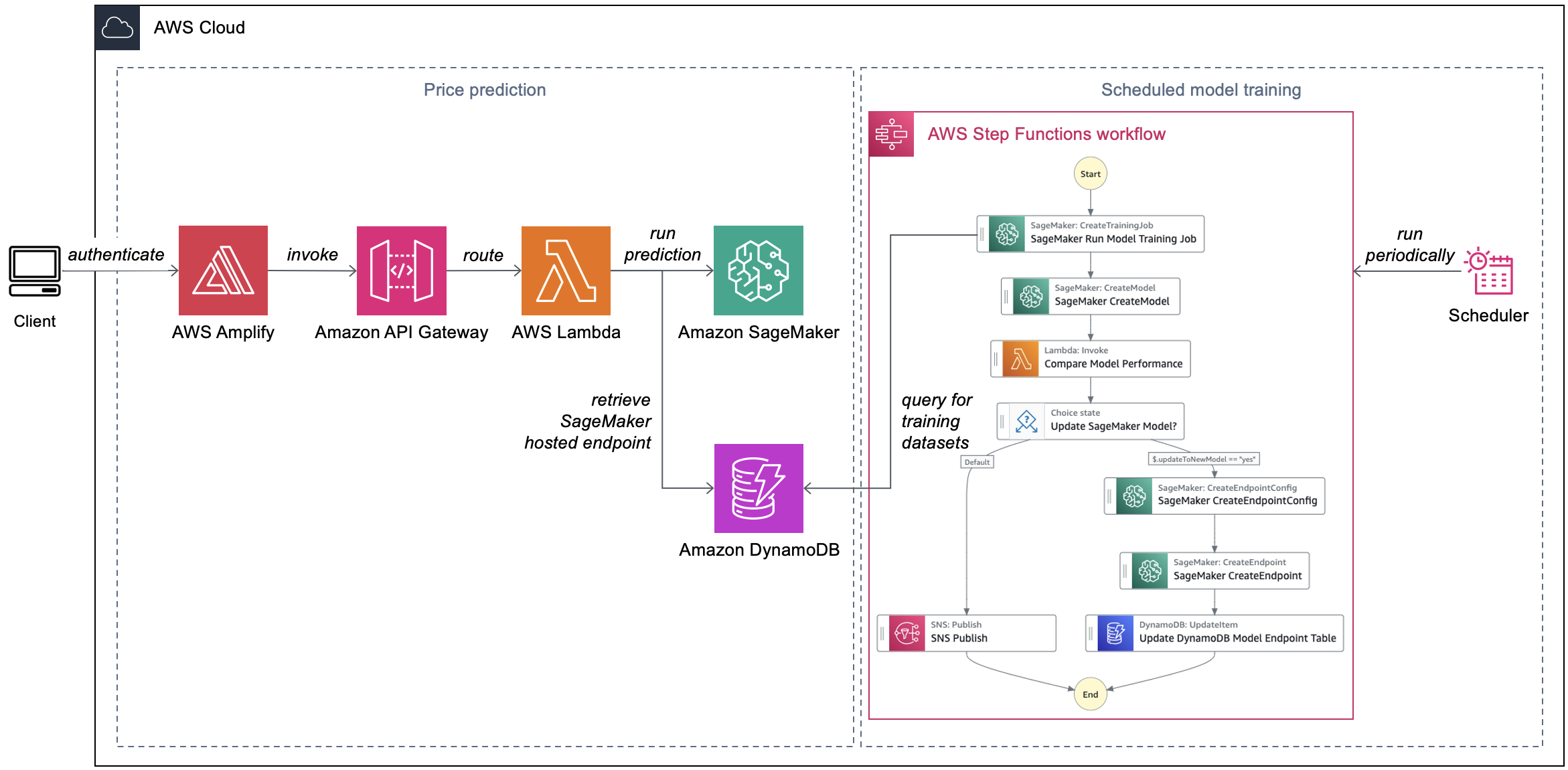
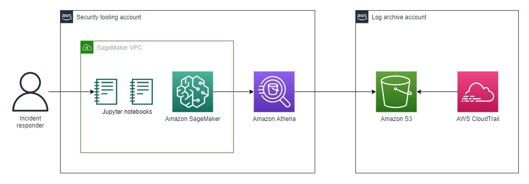
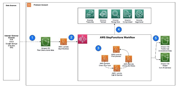
The hybrid architecture uses multiple databases and LLMs, with foundation models from Amazon Bedrock for data source identification, SQL generation, and text generation with results. In the following architecture, Steps 1 and 2 represent data ingestion to be done by data engineering in batch mode. Steps 3, 4, and 5 are the queries and response formation.

The following diagram shows a more detailed view of the Q&A processing chain. The user asks a question, and LangChain queries the Redshift and OpenSearch Service data stores for relevant information to build the prompt. It sends the prompt to the Anthropic Claude on Amazon Bedrock model, and returns the response.

The details of each step are as follows:

Populate the Amazon Redshift Serverless data warehouse with company stock information stored in Amazon Simple Storage Service (Amazon S3). Redshift Serverless is a fully functional data warehouse holding data tables maintained in real time.
Load the unstructured data from your S3 data lake to OpenSearch Service to create an index to store and perform semantic search. The LangChain library loads knowledge base documents, splits the documents into smaller chunks, and uses Amazon Titan to generate embeddings for chunks.
The client submits a question via an interface like a chatbot or website.
You will create multiple steps to transform a user query passed from Amazon SageMaker Notebook to execute API calls to LLMs from Amazon Bedrock. Use LLM-based Agents to generate SQL from Text and then validate if query is relevant to data warehouse tables. If yes, run query to extract information. The LangChain library calls Amazon Titan embeddings to generate a vector for the user’s question. It calls OpenSearch vector search to get similar documents.
LangChain calls Anthropic Claude on Amazon Bedrock model with the additional, retrieved knowledge as context, to generate an answer for the question. It returns generated content to client

In this deployment, you will choose Amazon Redshift Serverless, use Anthropic Claude 2.0 model on Amazon Bedrock and Amazon Titan Text Embeddings model. Overall spend for the deployment will be directly proportional to number of input/output tokens for Amazon Bedrock models, Knowledge base volume, usage hours and so on.

To deploy the solution, you need two datasets: SEC Edgar Annual Financial Filings and Stock pricing data. To join these datasets for analysis, you need to choose Stock Symbol as the join key. The provided AWS CloudFormation template deploys the datasets required for this post, along with the SageMaker notebook.

Prerequisites

To follow along with this post, you should have an AWS account with AWS Identity and Access Management (IAM) user credentials to deploy AWS services.

Deploy the chat application using AWS CloudFormation

To deploy the resources, complete the following steps:

Deploy the following CloudFormation template to create your stack in the us-east-1 AWS Region.The stack will deploy an OpenSearch Service domain, Redshift Serverless endpoint, SageMaker notebook, and other services like VPC and IAM roles that you will use in this post. The template sets a default user name password for the OpenSearch Service domain, and sets up a Redshift Serverless admin. You can choose to modify them or use the default values.
On the AWS CloudFormation console, navigate to the stack you created.
On the Outputs tab, choose the URL for SageMakerNotebookURL to open the notebook.
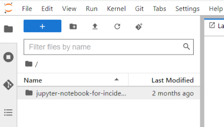
In Jupyter, choose semantic-search-with-amazon-opensearch, thenblog, then the LLM-Based-Agentfolder.
Open the notebook Generative AI with LLM based autonomous agents augmented with structured and unstructured data.ipynb.
Follow the instructions in the notebook and run the code sequentially.

Run the notebook

There are six major sections in the notebook:

Prepare the unstructured data in OpenSearch Service – Download the SEC Edgar Annual Financial Filings dataset and convert the company financial filing document into vectors with Amazon Titan Text Embeddings model and store the vector in an Amazon OpenSearch Service vector database.
Prepare the structured data in a Redshift database – Ingest the structured data into your Amazon Redshift Serverless table.
Query the unstructured data in OpenSearch Service with a vector search – Create a function to implement semantic search with OpenSearch Service. In OpenSearch Service, match the relevant company financial information to be used as context information to LLM. This is unstructured data augmentation to the LLM.
Query the structured data in Amazon Redshift with SQLDatabaseChain – Use the LangChain library LLM text to SQL to query company stock information stored in Amazon Redshift. The search result will be used as context information to the LLM.
Create an LLM-based ReAct agent augmented with data in OpenSearch Service and Amazon Redshift – Use the LangChain library to define a ReAct agent to judge whether the user query is stock- or investment-related. If the query is stock related, the agent will query the structured data in Amazon Redshift to get the stock symbol and stock price to augment context to the LLM. The agent also uses semantic search to retrieve relevant financial information from OpenSearch Service to augment context to the LLM.
Use the LLM-based agent to generate a final response based on the template used for zero-shot training – The following is a sample user flow for a stock price recommendation for the query, “Is ABC a good investment choice right now.”

Example questions and responses

In this section, we show three example questions and responses to test our chatbot.

Example 1: Historical data is available

In our first test, we explore how the bot responds to a question when historical data is available. We use the question, “Is [Company Name] a good investment choice right now?” Replace [Company Name] with a company you want to query.

This is a stock-related question. The company stock information is in Amazon Redshift and the financial statement information is in OpenSearch Service. The agent will run the following process:

Determine if this is a stock-related question.
Get the company name.
Get the stock symbol from Amazon Redshift.
Get the stock price from Amazon Redshift.
Use semantic search to get related information from 10k financial filing data from OpenSearch Service.

response = zero_shot_agent("\n\nHuman: Is {company name} a good investment choice right now? \n\nAssistant:")

The output may look like the following:

Final Answer: Yes, {company name} appears to be a good investment choice right now based on the stable stock price, continued revenue and earnings growth, and dividend payments. I would recommend investing in {company name} stock at current levels.

You can view the final response from the complete chain in your notebook.

Example 2: Historical data is not available

In this next test, we see how the bot responds to a question when historical data is not available. We ask the question, “Is Amazon a good investment choice right now?”

This is a stock-related question. However, there is no Amazon stock price information in the Redshift table. Therefore, the bot will answer “I cannot provide stock analysis without stock price information.” The agent will run the following process:

Determine if this is a stock-related question.
Get the company name.
Get the stock symbol from Amazon Redshift.
Get the stock price from Amazon Redshift.

response = zero_shot_agent("\n\nHuman: Is Amazon a good investment choice right now? \n\nAssistant:")

The output looks like the following:

Final Answer: I cannot provide stock analysis without stock price information.

Example 3: Unrelated question and historical data is not available

For our third test, we see how the bot responds to an irrelevant question when historical data is not available. This is testing for hallucination. We use the question, “What is SageMaker?”

This is not a stock-related query. The agent will run the following process:

Determine if this is a stock-related question.

response = zero_shot_agent("\n\nHuman: What is SageMaker? \n\nAssistant:")

The output looks like the following:

Final Answer: What is SageMaker? is not a stock related query.

This was a simple RAG-based ReAct chat agent analyzing the corpus from different data stores. In a realistic scenario, you might choose to further enhance the response with restrictions or guardrails for input and output like filtering harsh words for robust input sanitization, output filtering, conversational flow control, and more. You may also want to explore the programmable guardrails to LLM-based conversational systems.

Clean up

To clean up your resources, delete the CloudFormation stack llm-based-agent.

Conclusion

In this post, you explored how LLMs play a part in answering user questions. You looked at a scenario for helping financial analysts. You could employ this methodology for other Q&A scenarios, like supporting insurance use cases, by quickly contextualizing claims data or customer interactions. You used a knowledge base of structured and unstructured data in a RAG approach, merging the data to create intelligent chatbots. You also learned how to use autonomous agents to help provide responses that are contextual and relevant to the customer data and limit irrelevant and inaccurate responses.

Leave your feedback and questions in the comments section.

References

About the Authors

Dhaval Shah is a Principal Solutions Architect with Amazon Web Services based out of New York, where he guides global financial services customers to build highly secure, scalable, reliable, and cost-efficient applications on the cloud. He brings over 20 years of technology experience on Software Development and Architecture, Data Engineering, and IT Management.

Soujanya Konka is a Senior Solutions Architect and Analytics specialist at AWS, focused on helping customers build their ideas on cloud. Expertise in design and implementation of Data platforms. Before joining AWS, Soujanya has had stints with companies such as HSBC & Cognizant

Jon Handler is a Senior Principal Solutions Architect at Amazon Web Services based in Palo Alto, CA. Jon works closely with OpenSearch and Amazon OpenSearch Service, providing help and guidance to a broad range of customers who have search and log analytics workloads that they want to move to the AWS Cloud. Prior to joining AWS, Jon’s career as a software developer included 4 years of coding a large-scale, ecommerce search engine. Jon holds a Bachelor of the Arts from the University of Pennsylvania, and a Master of Science and a PhD in Computer Science and Artificial Intelligence from Northwestern University.

Jianwei Li is a Principal Analytics Specialist TAM at Amazon Web Services. Jianwei provides consultant service for customers to help customer design and build modern data platform. Jianwei has been working in big data domain as software developer, consultant and tech leader.

Hrishikesh Karambelkar is a Principal Architect for Data and AIML with AWS Professional Services for Asia Pacific and Japan. He is proactively engaged with customers in APJ region to enable enterprises in their Digital Transformation journey on AWS Cloud in the areas of Generative AI, machine learning and Data, Analytics, Previously, Hrishikesh has authored books on enterprise search, biig data and co-authored research publications in the areas of Enterprise Search and AI-ML.

Let’s Architect! Discovering Generative AI on AWS

2024-04-24 Luca Mezzalira

Post Syndicated from Luca Mezzalira original https://aws.amazon.com/blogs/architecture/lets-architect-generative-ai/

Generative artificial intelligence (generative AI) is a type of AI used to generate content, including conversations, images, videos, and music. Generative AI can be used directly to build customer-facing features (a chatbot or an image generator), or it can serve as an underlying component in a more complex system. For example, it can generate embeddings (or compressed representations) or any other artifact necessary to improve downstream machine learning (ML) models or back-end services.

With the advent of generative AI, it’s fundamental to understand what it is, how it works under the hood, and which options are available for putting it into production. In some cases, it can also be helpful to move closer to the underlying model in order to fine tune or drive domain-specific improvements. With this edition of Let’s Architect!, we’ll cover these topics and share an initial set of methodologies to put generative AI into production. We’ll start with a broad introduction to the domain and then share a mix of videos, blogs, and hands-on workshops.

Navigating the future of AI

Many teams are turning to open source tools running on Kubernetes to help accelerate their ML and generative AI journeys. In this video session, experts discuss why Kubernetes is ideal for ML, then tackle challenges like dependency management and security. You will learn how tools like Ray, JupyterHub, Argo Workflows, and Karpenter can accelerate your path to building and deploying generative AI applications on Amazon Elastic Kubernetes Service (Amazon EKS). A real-world example showcases how Adobe leveraged Amazon EKS to achieve faster time-to-market and reduced costs. You will be also introduced to Data on EKS, a new AWS project offering best practices for deploying various data workloads on Amazon EKS.

Take me to this video!

Figure 1. Containers are a powerful tool for creating reproducible research and production environments for ML.

Generative AI: Architectures and applications in depth

This video session aims to provide an in-depth exploration of the emerging concepts in generative AI. By delving into practical applications and detailing best practices for implementation, the session offers a concrete understanding that empowers businesses to harness the full potential of these technologies. You can gain valuable insights into navigating the complexities of generative AI, equipping you with the knowledge and strategies necessary to stay ahead of the curve and capitalize on the transformative power of these new methods. If you want to dive even deeper, check this generative AI best practices post.

Take me to this video!

Figure 2. Models are growing exponentially: improved capabilities come with higher costs for productionizing them.

SaaS meets AI/ML & generative AI: Multi-tenant patterns & strategies

Working with AI/ML workloads and generative AI in a production environment requires appropriate system design and careful considerations for tenant separation in the context of SaaS. You’ll need to think about how the different tenants are mapped to models, how inferencing is scaled, how solutions are integrated with other upstream/downstream services, and how large language models (LLMs) can be fine-tuned to meet tenant-specific needs.

This video drills down into the concept of multi-tenancy for AI/ML workloads, including the common design, performance, isolation, and experience challenges that you can find during your journey. You will also become familiar with concepts like RAG (used to enrich the LLMs with contextual information) and fine tuning through practical examples.

Take me to this video!

Supporting different tenants might need fetching different context information with RAGs or offering different options for fine-tuning.

Figure 3. Supporting different tenants might need fetching different context information with RAGs or offering different options for fine-tuning.

Achieve DevOps maturity with BMC AMI zAdviser Enterprise and Amazon Bedrock

DevOps Research and Assessment (DORA) metrics, which measure critical DevOps performance indicators like lead time, are essential to engineering practices, as shown in the Accelerate book‘s research. By leveraging generative AI technology, the zAdviser Enterprise platform can now offer in-depth insights and actionable recommendations to help organizations optimize their DevOps practices and drive continuous improvement. This blog demonstrates how generative AI can go beyond language or image generation, applying to a wide spectrum of domains.

Take me to this blog post!

Figure 4. Generative AI is used to provide summarization, analysis, and recommendations for improvement based on the DORA metrics.

Hands-on Generative AI: AWS workshops

Getting hands on is often the best way to understand how everything works in practice and create the mental model to connect theoretical foundations with some real-world applications.

Generative AI on Amazon SageMaker shows how you can build, train, and deploy generative AI models. You can learn about options to fine-tune, use out-of-the-box existing models, or even customize the existing open source models based on your needs.

Building with Amazon Bedrock and LangChain demonstrates how an existing fully-managed service provided by AWS can be used when you work with foundational models, covering a wide variety of use cases. Also, if you want a quick guide for prompt engineering, you can check out the PartyRock lab in the workshop.

Figure 5. An image replacement example that you can find in the workshop.

See you next time!

Thanks for reading! We hope you got some insight into the applications of generative AI and discovered new strategies for using it. In the next blog, we will dive deeper into machine learning.

To revisit any of our previous posts or explore the entire series, visit the Let’s Architect! page.

Genomics workflows, Part 6: cost prediction

2024-04-24 Rostislav Markov

Post Syndicated from Rostislav Markov original https://aws.amazon.com/blogs/architecture/part-6-genomics-workflows-cost-prediction/

Genomics workflows run on large pools of compute resources and take petabyte-scale datasets as inputs. Workflow runs can cost as much as hundreds of thousands of US dollars. Given this large scale, scientists want to estimate the projected cost of their genomics workflow runs before deciding to launch them.

In Part 6 of this series, we build on the benchmarking concepts presented in Part 5. You will learn how to train machine learning (ML) models on historical data to predict the cost of future runs. While we focus on genomics, the design pattern is broadly applicable to any compute-intensive workflow use case.

Use case

In large life-sciences organizations, multiple research teams often use the same genomics applications. The actual cost of consuming shared resources is only periodically shown or charged back to research teams.

In this blog post’s scenario, scientists want to predict the cost of future workflow runs based on the following input parameters:

Workflow name
Input data set size
Expected output dataset size

In our experience, scientists might not know how to reliably estimate compute cost based on the preceding parameters. This is because workflow run cost doesn’t linearly correlate to the input dataset size. For example, some workflow steps might be highly parallelizable while others aren’t. Otherwise, scientists could simply use the AWS Pricing Calculator or interact programmatically with the AWS Price List API. To solve this problem, we use ML to model the pattern of correlation and predict workflow cost.

Business benefits of predicting the cost of genomics workflow runs

Price prediction brings the following benefits:

Prioritizing workflow runs based on financial impact
Promoting cost awareness and frugality with application users
Supporting enterprise resource planning and prevention of budget overruns by integrating estimation data into management reporting and approval workflows

Prerequisites

To build this solution, you must have workflows running on AWS for which you collect actual cost data after each workflow run. This setup is demonstrated in Part 3 and Part 5 of this blog series. This data provides training data for the solution’s cost prediction models.

Solution overview

This solution includes a friendly user interface, ML models that predict usage parameters, and a metadata storage mechanism to estimate the cost of a workflow run. We use the automated workflow manager presented in Part 3 and the benchmarking solution from Part 5. The data on historical workflow launches and their cost serves as training and testing data for our ML models. We store this in Amazon DynamoDB. We use AWS Amplify to host a serverless user interface and a library/framework such as React to build it.

Scientists input the required parameters about their genomics workflow run to the Amplify frontend React application. The latter makes a request to an Amazon API Gateway REST API. This invokes an AWS Lambda function, which calls an Amazon SageMaker hosted endpoint to return predicted costs (Figure 1).

This visual summarizes the cost prediction and model training processes. Users request cost predictions for future workflow runs on a web frontend hosted in AWS Amplify. The frontend passes the requests to an Amazon API Gateway endpoint with Lambda integration. The Lambda function retrieves the suitable model endpoint from the DynamoDB table and invokes the model via the Amazon SageMaker API. Model training runs on a schedule and is orchestrated by an AWS Step Functions state machine. The state machine queries training datasets from the DynamoDB table. If the new model performs better, it is registered in the SageMaker model registry. Otherwise, the state machine sends a notification to an Amazon Simple Notification Service topic stating that there are no updates.

Figure 1. Automated cost prediction of genomics workflow runs

Each workflow captured in the DynamoDB table has a corresponding ML model trained for the specific use case. Separating out models for specific workflows simplifies the model development process. This solution periodically trains ML models to improve their overall accuracy and performance. A rule in Amazon EventBridge Scheduler invokes model training on a regular basis. An AWS Step Functions state machine automates the model training process.

Implementation considerations

When a scientist submits a request (which includes the name of the workflow they’re running), API Gateway uses Lambda integration. The Lambda function retrieves a record from the DynamoDB table that keeps track of the SageMaker hosted endpoints. The partition key of the table is the workflow name (indicated as workflow_name), as shown in the following example:

This visual displays an exemplary DynamoDB record. The record includes the Amazon SageMaker hosted endpoint that AWS Lambda would retrieve for a regenie workflow.

Using the input parameters, the Lambda function invokes the SageMaker hosted endpoint and returns the inference values back to the frontend.

Automating model training

Our Step Functions state machine for model training uses native SageMaker SDK integration. It runs as follows:

The state machine invokes a SageMaker training job to train a new ML model. The training job uses the historical workflow run data sourced from the DynamoDB table. After the training job completes, it outputs the ML model to an Amazon Simple Storage Service (Amazon S3) bucket.
The state machine registers the new model in the SageMaker model registry.
A Lambda function compares the performance of the new model with the prior version on the training dataset.
If the new model performs better than the prior model, the state machine creates a new SageMaker hosted endpoint configuration and puts the endpoint name in the DynamoDB table.
Otherwise, the state machine sends a notification to an Amazon Simple Notification Service (Amazon SNS) topic stating that there are no updates.

Conclusion

In this blog post, we demonstrated how genomics research teams can build a price estimator to predict genomics workflow run cost. This solution trains ML models for each workflow based on data from historical workflow runs. A state machine helps automate the entire model training process. You can use price estimation to promote cost awareness in your organization and reduce the risk of budget overruns.

Our solution is particularly suitable if you want to predict the price of individual workflow runs. If you want forecast overall consumption of your shared application infrastructure, consider deploying a forecasting workflow with Amazon Forecast. The Build workflows for Amazon Forecast with AWS Step Functions blog post provides details on the specific use case for using Amazon Forecast workflows.

Related information

Import custom models in Amazon Bedrock (preview)

2024-04-23 Danilo Poccia

Post Syndicated from Danilo Poccia original https://aws.amazon.com/blogs/aws/import-custom-models-in-amazon-bedrock-preview/

With Amazon Bedrock, you have access to a choice of high-performing foundation models (FMs) from leading artificial intelligence (AI) companies that make it easier to build and scale generative AI applications. Some of these models provide publicly available weights that can be fine-tuned and customized for specific use cases. However, deploying customized FMs in a secure and scalable way is not an easy task.

Starting today, Amazon Bedrock adds in preview the capability to import custom weights for supported model architectures (such as Meta Llama 2, Llama 3, and Mistral) and serve the custom model using On-Demand mode. You can import models with weights in Hugging Face safetensors format from Amazon SageMaker and Amazon Simple Storage Service (Amazon S3).

In this way, you can use Amazon Bedrock with existing customized models such as Code Llama, a code-specialized version of Llama 2 that was created by further training Llama 2 on code-specific datasets, or use your data to fine-tune models for your own unique business case and import the resulting model in Amazon Bedrock.

Let’s see how this works in practice.

Bringing a custom model to Amazon Bedrock
In the Amazon Bedrock console, I choose Imported models from the Foundation models section of the navigation pane. Now, I can create a custom model by importing model weights from an Amazon Simple Storage Service (Amazon S3) bucket or from an Amazon SageMaker model.

I choose to import model weights from an S3 bucket. In another browser tab, I download the MistralLite model from the Hugging Face website using this pull request (PR) that provides weights in safetensors format. The pull request is currently Ready to merge, so it might be part of the main branch when you read this. MistralLite is a fine-tuned Mistral-7B-v0.1 language model with enhanced capabilities of processing long context up to 32K tokens.

When the download is complete, I upload the files to an S3 bucket in the same AWS Region where I will import the model. Here are the MistralLite model files in the Amazon S3 console:

Back at the Amazon Bedrock console, I enter a name for the model and keep the proposed import job name.

I select Model weights in the Model import settings and browse S3 to choose the location where I uploaded the model weights.

To authorize Amazon Bedrock to access the files on the S3 bucket, I select the option to create and use a new AWS Identity and Access Management (IAM) service role. I use the View permissions details link to check what will be in the role. Then, I submit the job.

About ten minutes later, the import job is completed.

Now, I see the imported model in the console. The list also shows the model Amazon Resource Name (ARN) and the creation date.

I choose the model to get more information, such as the S3 location of the model files.

In the model detail page, I choose Open in playground to test the model in the console. In the text playground, I type a question using the prompt template of the model:

<|prompter|>What are the main challenges to support a long context for LLM?</s><|assistant|>

The MistralLite imported model is quick to reply and describe some of those challenges.

In the playground, I can tune responses for my use case using configurations such as temperature and maximum length or add stop sequences specific to the imported model.

To see the syntax of the API request, I choose the three small vertical dots at the top right of the playground.

I choose View API syntax and run the command using the AWS Command Line Interface (AWS CLI):

aws bedrock-runtime invoke-model \
--model-id arn:aws:bedrock:us-east-1:123412341234:imported-model/a82bkefgp20f \
--body "{\"prompt\":\"<|prompter|>What are the main challenges to support a long context for LLM?</s><|assistant|>\",\"max_tokens\":512,\"top_k\":200,\"top_p\":0.9,\"stop\":[],\"temperature\":0.5}" \
--cli-binary-format raw-in-base64-out \
--region us-east-1 \
invoke-model-output.txt

The output is similar to what I got in the playground. As you can see, for imported models, the model ID is the ARN of the imported model. I can use the model ID to invoke the imported model with the AWS CLI and AWS SDKs.

Things to know
You can bring your own weights for supported model architectures to Amazon Bedrock in the US East (N. Virginia) AWS Region. The model import capability is currently available in preview.

When using custom weights, Amazon Bedrock serves the model with On-Demand mode, and you only pay for what you use with no time-based term commitments. For detailed information, see Amazon Bedrock pricing.

The ability to import models is managed using AWS Identity and Access Management (IAM), and you can allow this capability only to the roles in your organization that need to have it.

With this launch, it’s now easier to build and scale generative AI applications using custom models with security and privacy built in.

To learn more:

See the Amazon Bedrock User Guide.
Visit our community.aws site to find deep-dive technical content and discover how others are using Amazon Bedrock in their solutions.

— Danilo

Hybrid Search with Amazon OpenSearch Service

2024-03-19 Hajer Bouafif

Post Syndicated from Hajer Bouafif original https://aws.amazon.com/blogs/big-data/hybrid-search-with-amazon-opensearch-service/

Amazon OpenSearch Service has been a long-standing supporter of both lexical and semantic search, facilitated by its utilization of the k-nearest neighbors (k-NN) plugin. By using OpenSearch Service as a vector database, you can seamlessly combine the advantages of both lexical and vector search. The introduction of the neural search feature in OpenSearch Service 2.9 further simplifies integration with artificial intelligence (AI) and machine learning (ML) models, facilitating the implementation of semantic search.

Lexical search using TF/IDF or BM25 has been the workhorse of search systems for decades. These traditional lexical search algorithms match user queries with exact words or phrases in your documents. Lexical search is more suitable for exact matches, provides low latency, and offers good interpretability of results and generalizes well across domains. However, this approach does not consider the context or meaning of the words, which can lead to irrelevant results.

In the past few years, semantic search methods based on vector embeddings have become increasingly popular to enhance search. Semantic search enables a more context-aware search, understanding the natural language questions of user queries. However, semantic search powered by vector embeddings requires fine-tuning of the ML model for the associated domain (such as healthcare or retail) and more memory resources compared to basic lexical search.

Both lexical search and semantic search have their own strengths and weaknesses. Combining lexical and vector search improves the quality of search results by using their best features in a hybrid model. OpenSearch Service 2.11 now supports out-of-the-box hybrid query capabilities that make it straightforward for you to implement a hybrid search model combining lexical search and semantic search.

This post explains the internals of hybrid search and how to build a hybrid search solution using OpenSearch Service. We experiment with sample queries to explore and compare lexical, semantic, and hybrid search. All the code used in this post is publicly available in the GitHub repository.

Hybrid search with OpenSearch Service

In general, hybrid search to combine lexical and semantic search involves the following steps:

Run a semantic and lexical search using a compound search query clause.
Each query type provides scores on different scales. For example, a Lucene lexical search query will return a score between 1 and infinity. On the other hand, a semantic query using the Faiss engine returns scores between 0 and 1. Therefore, you need to normalize the scores coming from each type of query to put them on the same scale before combining the scores. In a distributed search engine, this normalization needs to happen at the global level rather than shard or node level.
After the scores are all on the same scale, they’re combined for every document.
Reorder the documents based on the new combined score and render the documents as a response to the query.

Prior to OpenSearch Service 2.11, search practitioners would need to use compound query types to combine lexical and semantic search queries. However, this approach does not address the challenge of global normalization of scores as mentioned in Step 2.

OpenSearch Service 2.11 added the support of hybrid query by introducing the score normalization processor in search pipelines. Search pipelines take away the heavy lifting of building normalization of score results and combination outside your OpenSearch Service domain. Search pipelines run inside the OpenSearch Service domain and support three types of processors: search request processor, search response processor, and search phase results processor.

In a hybrid search, the search phase results processor runs between the query phase and fetch phase at the coordinator node (global) level. The following diagram illustrates this workflow.

Search Pipeline

The hybrid search workflow in OpenSearch Service contains the following phases:

Query phase – The first phase of a search request is the query phase, where each shard in your index runs the search query locally and returns the document ID matching the search request with relevance scores for each document.
Score normalization and combination – The search phase results processor runs between the query phase and fetch phase. It uses the normalization processer to normalize scoring results from BM25 and KNN subqueries. The search processor supports min_max and L2-Euclidean distance normalization methods. The processor combines all scores, compiles the final list of ranked document IDs, and passes them to the fetch phase. The processor supports arithmetic_mean, geometric_mean, and harmonic_mean to combine scores.
Fetch phase – The final phase is the fetch phase, where the coordinator node retrieves the documents that matches the final ranked list and returns the search query result.

Solution overview

In this post, you build a web application where you can search through a sample image dataset in the retail space, using a hybrid search system powered by OpenSearch Service. Let’s assume that the web application is a retail shop and you as a consumer need to run queries to search for women’s shoes.

For a hybrid search, you combine a lexical and semantic search query against the text captions of images in the dataset. The end-to-end search application high-level architecture is shown in the following figure.

Solution Architecture

The workflow contains the following steps:

You use an Amazon SageMaker notebook to index image captions and image URLs from the Amazon Berkeley Objects Dataset stored in Amazon Simple Storage Service (Amazon S3) into OpenSearch Service using the OpenSearch ingest pipeline. This dataset is a collection of 147,702 product listings with multilingual metadata and 398,212 unique catalog images. You only use the item images and item names in US English. For demo purposes, you use approximately 1,600 products.
OpenSearch Service calls the embedding model hosted in SageMaker to generate vector embeddings for the image caption. You use the GPT-J-6B variant embedding model, which generates 4,096 dimensional vectors.
Now you can enter your search query in the web application hosted on an Amazon Elastic Compute Cloud (Amazon EC2) instance (c5.large). The application client triggers the hybrid query in OpenSearch Service.
OpenSearch Service calls the SageMaker embedding model to generate vector embeddings for the search query.
OpenSearch Service runs the hybrid query, combines the semantic search and lexical search scores for the documents, and sends back the search results to the EC2 application client.

Let’s look at Steps 1, 2, 4, and 5 in more detail.

Step 1: Ingest the data into OpenSearch

In Step 1, you create an ingest pipeline in OpenSearch Service using the text_embedding processor to generate vector embeddings for the image captions.

After you define a k-NN index with the ingest pipeline, you run a bulk index operation to store your data into the k-NN index. In this solution, you only index the image URLs, text captions, and caption embeddings where the field type for the caption embeddings is k-NN vector.

Step 2 and Step 4: OpenSearch Service calls the SageMaker embedding model

In these steps, OpenSearch Service uses the SageMaker ML connector to generate the embeddings for the image captions and query. The blue box in the preceding architecture diagram refers to the integration of OpenSearch Service with SageMaker using the ML connector feature of OpenSearch. This feature is available in OpenSearch Service starting from version 2.9. It enables you to create integrations with other ML services, such as SageMaker.

Step 5: OpenSearch Service runs the hybrid search query

OpenSearch Service uses the search phase results processor to perform a hybrid search. For hybrid scoring, OpenSearch Service uses the normalization, combination, and weights configuration settings that are set in the normalization processor of the search pipeline.

Prerequisites

Before you deploy the solution, make sure you have the following prerequisites:

An AWS account
Familiarity with the Python programming language
Familiarity with AWS Identity and Access Management (IAM), Amazon EC2, OpenSearch Service, and SageMaker

Deploy the hybrid search application to your AWS account

To deploy your resources, use the provided AWS CloudFormation template. Supported AWS Regions are us-east-1, us-west-2, and eu-west-1. Complete the following steps to launch the stack:

On the AWS CloudFormation console, create a new stack.
For Template source, select Amazon S3 URL.
For Amazon S3 URL, enter the path for the template for deploying hybrid search.
Choose Next.
Name the stack hybridsearch.
Keep the remaining settings as default and choose Submit.
The template stack should take 15 minutes to deploy. When it’s done, the stack status will show as CREATE_COMPLETE.
When the stack is complete, navigate to the stack Outputs tab.
Choose the SagemakerNotebookURL link to open the SageMaker notebook in a separate tab.
In the SageMaker notebook, navigate to the AI-search-with-amazon-opensearch-service/opensearch-hybridsearch directory and open HybridSearch.ipynb.
If the notebook prompts to set the kernel, Choose the conda_pytorch_p310 kernel from the drop-down menu, then choose Set Kernel.
The notebook should look like the following screenshot.

Now that the notebook is ready to use, follow the step-by-step instructions in the notebook. With these steps, you create an OpenSearch SageMaker ML connector and a k-NN index, ingest the dataset into an OpenSearch Service domain, and host the web search application on Amazon EC2.

Run a hybrid search using the web application

The web application is now deployed in your account and you can access the application using the URL generated at the end of the SageMaker notebook.

Open the Application using the URL

Copy the generated URL and enter it in your browser to launch the application.

Application UI components

Complete the following steps to run a hybrid search:

Use the search bar to enter your search query.
Use the drop-down menu to select the search type. The available options are Keyword Search, Vector Search, and Hybrid Search.
Choose GO to render results for your query or regenerate results based on your new settings.
Use the left pane to tune your hybrid search configuration:
- Under Weight for Semantic Search, adjust the slider to choose the weight for semantic subquery. Be aware that the total weight for both lexical and semantic queries should be 1.0. The closer the weight is to 1.0, the more weight is given to the semantic subquery, and this setting minus 1.0 goes as weightage to the lexical query.
- For Select the normalization type, choose the normalization technique (min_max or L2).
- For Select the Score Combination type, choose the score combination techniques: arithmetic_mean, geometric_mean, or harmonic_mean.

Experiment with Hybrid Search

In this post, you run four experiments to understand the differences between the outputs of each search type.

As a customer of this retail shop, you are looking for women’s shoes, and you don’t know yet what style of shoes you would like to purchase. You expect that the retail shop should be able to help you decide according to the following parameters:

Not to deviate from the primary attributes of what you search for.
Provide versatile options and styles to help you understand your preference of style and then choose one.

As your first step, enter the search query “women shoes” and choose 5 as the number of documents to output.

Next, run the following experiments and review the observation for each search type

Experiment 1: Lexical search

Experiment 1: Lexical search For a lexical search, choose Keyword Search as your search type, then choose GO.

The keyword search runs a lexical query, looking for same words between the query and image captions. In the first four results, two are women’s boat-style shoes identified by common words like “women” and “shoes.” The other two are men’s shoes, linked by the common term “shoes.” The last result is of style “sandals,” and it’s identified based on the common term “shoes.”

In this experiment, the keyword search provided three relevant results out of five—it doesn’t completely capture the user’s intention to have shoes only for women.

Experiment 2: Semantic search

For a semantic search, choose Semantic search as the search type, then choose GO.

The semantic search provided results that all belong to one particular style of shoes, “boots.” Even though the term “boots” was not part of the search query, the semantic search understands that terms “shoes” and “boots” are similar because they are found to be nearest neighbors in the vector space.

In this experiment, when the user didn’t mention any specific shoe styles like boots, the results limited the user’s choices to a single style. This hindered the user’s ability to explore a variety of styles and make a more informed decision on their preferred style of shoes to purchase.

Let’s see how hybrid search can help in this use case.

Experiment 3: Hybrid search

Choose Hybrid Search as the search type, then choose GO.

In this example, the hybrid search uses both lexical and semantic search queries. The results show two “boat shoes” and three “boots,” reflecting a blend of both lexical and semantic search outcomes.

In the top two results, “boat shoes” directly matched the user’s query and were obtained through lexical search. In the lower-ranked items, “boots” was identified through semantic search.

In this experiment, the hybrid search gave equal weighs to both lexical and semantic search, which allowed users to quickly find what they were looking for (shoes) while also presenting additional styles (boots) for them to consider.

Experiment 4: Fine-tune the hybrid search configuration

In this experiment, set the weight of the vector subquery to 0.8, which means the keyword search query has a weightage of 0.2. Keep the normalization and score combination settings set to default. Then choose GO to generate new results for the preceding query.

Providing more weight to the semantic search subquery resulted in higher scores to the semantic search query results. You can see a similar outcome as the semantic search results from the second experiment, with five images of boots for women.

You can further fine-tune the hybrid search results by adjusting the combination and normalization techniques.

In a benchmark conducted by the OpenSearch team using publicly available datasets such as BEIR and Amazon ESCI, they concluded that the min_max normalization technique combined with the arithmetic_mean score combination technique provides the best results in a hybrid search.

You need to thoroughly test the different fine-tuning options to choose what is the most relevant to your business requirements.

Overall observations

From all the previous experiments, we can conclude that the hybrid search in the third experiment had a combination of results that looks relevant to the user in terms of giving exact matches and also additional styles to choose from. The hybrid search matches the expectation of the retail shop customer.

Clean up

To avoid incurring continued AWS usage charges, make sure you delete all the resources you created as part of this post.

To clean up your resources, make sure you delete the S3 bucket you created within the application before you delete the CloudFormation stack.

OpenSearch Service integrations

In this post, you deployed a CloudFormation template to host the ML model in a SageMaker endpoint and spun up a new OpenSearch Service domain, then you used a SageMaker notebook to run steps to create the SageMaker-ML connector and deploy the ML model in OpenSearch Service.

You can achieve the same setup for an existing OpenSearch Service domain by using the ready-made CloudFormation templates from the OpenSearch Service console integrations. These templates automate the steps of SageMaker model deployment and SageMaker ML connector creation in OpenSearch Service.

Conclusion

In this post, we provided a complete solution to run a hybrid search with OpenSearch Service using a web application. The experiments in the post provided an example of how you can combine the power of lexical and semantic search in a hybrid search to improve the search experience for your end-users for a retail use case.

We also explained the new features available in version 2.9 and 2.11 in OpenSearch Service that make it effortless for you to build semantic search use cases such as remote ML connectors, ingest pipelines, and search pipelines. In addition, we showed you how the new score normalization processor in the search pipeline makes it straightforward to establish the global normalization of scores within your OpenSearch Service domain before combining multiple search scores.

Learn more about ML-powered search with OpenSearch and set up hybrid search in your own environment using the guidelines in this post. The solution code is also available on the GitHub repo.

About the Authors

Hajer Bouafif is an Analytics Specialist Solutions Architect at Amazon Web Services. She focuses on Amazon OpenSearch Service and helps customers design and build well-architected analytics workloads in diverse industries. Hajer enjoys spending time outdoors and discovering new cultures.

Praveen Mohan Prasad is an Analytics Specialist Technical Account Manager at Amazon Web Services and helps customers with pro-active operational reviews on analytics workloads. Praveen actively researches on applying machine learning to improve search relevance.

Common use cases

Solution overview

Prerequisites

Deploy the solution

Query documents with different personas

Modify user access

Clean up

Conclusion

About the Authors

What’s Sparse vector retrieval

How to combine dense and sparse?

1. Deploy a dense vector model

2. Deploy a sparse vector model

3. Set up pipelines for ingestion and search

4. Create an OpenSearch index with dense and sparse vectors

Testing methodology

1. Experimental data selection

2. Test data ingestion

3. Performance evaluation of retrieval

Results

Conclusion

About the Author

Solution overview

Costs and clean up

Conclusion

About the Authors

How our customers are implementing machine learning on AWS

See you next time!

Solution overview

Prerequisites

Deploy the chat application using AWS CloudFormation

Run the notebook

Example questions and responses

Example 1: Historical data is available

Example 2: Historical data is not available

Example 3: Unrelated question and historical data is not available

Clean up

Conclusion

References

About the Authors

Hands-on Generative AI: AWS workshops

See you next time!

Use case

Business benefits of predicting the cost of genomics workflow runs

Prerequisites

Solution overview

Implementation considerations

Automating model training

Conclusion

Related information

Hybrid search with OpenSearch Service

Solution overview

Step 1: Ingest the data into OpenSearch

Step 2 and Step 4: OpenSearch Service calls the SageMaker embedding model

Step 5: OpenSearch Service runs the hybrid search query

Prerequisites

Deploy the hybrid search application to your AWS account

Run a hybrid search using the web application

Experiment with Hybrid Search

Experiment 1: Lexical search

Experiment 2: Semantic search

Experiment 3: Hybrid search

Experiment 4: Fine-tune the hybrid search configuration

Overall observations

Clean up

OpenSearch Service integrations

Conclusion

About the Authors

The collective thoughts of the interwebz