Tag Archives: Customer Solutions

Enable business users to analyze large datasets in your data lake with Amazon QuickSight

Post Syndicated from Eliad Maimon original https://aws.amazon.com/blogs/big-data/enable-business-users-to-analyze-large-datasets-in-your-data-lake-with-amazon-quicksight/

This blog post is co-written with Ori Nakar from Imperva.

Imperva Cloud WAF protects hundreds of thousands of websites and blocks billions of security events every day. Events and many other security data types are stored in Imperva’s Threat Research Multi-Region data lake.

Imperva harnesses data to improve their business outcomes. To enable this transformation to a data-driven organization, Imperva brings together data from structured, semi-structured, and unstructured sources into a data lake. As part of their solution, they are using Amazon QuickSight to unlock insights from their data.

Imperva’s data lake is based on Amazon Simple Storage Service (Amazon S3), where data is continually loaded. Imperva’s data lake has a few dozen different datasets, in the scale of petabytes. Each day, TBs of new data is added to the data lake, which is then transformed, aggregated, partitioned, and compressed.

In this post, we explain how Imperva’s solution enables users across the organization to explore, visualize, and analyze data using Amazon Redshift Serverless, Amazon Athena, and QuickSight.

Challenges and needs

A modern data strategy gives you a comprehensive plan to manage, access, analyze, and act on data. AWS provides the most complete set of services for the entire end-to-end data journey for all workloads, all types of data, and all desired business outcomes. In turn, this makes AWS the best place to unlock value from your data and turn it into insight.

Redshift Serverless is a serverless option of Amazon Redshift that allows you to run and scale analytics without having to provision and manage data warehouse clusters. Redshift Serverless automatically provisions and intelligently scales data warehouse capacity to deliver high performance for all your analytics. You just need to load and query your data, and you only pay for the compute used for the duration of the workloads on a per-second basis. Redshift Serverless is ideal when it’s difficult to predict compute needs such as variable workloads, periodic workloads with idle time, and steady-state workloads with spikes.

Athena is an interactive query service that makes it easy to analyze data in Amazon S3 using standard SQL. Athena is serverless, straightforward to use, and makes it simple for anyone with SQL skills to quickly analyze large-scale datasets in multiple Regions.

QuickSight is a cloud-native business intelligence (BI) service that you can use to visually analyze data and share interactive dashboards with all users in the organization. QuickSight is fully managed and serverless, requires no client downloads for dashboard creation, and has a pay-per-session pricing model that allows you to pay for dashboard consumption. Imperva uses QuickSight to enable users with no technical expertise, from different teams such as marketing, product, sales, and others, to extract insight from the data without the help of data or research teams.

QuickSight offers SPICE, an in-memory, cloud-native data store that allows end-users to interactively explore data. SPICE provides consistently fast query performance and automatically scales for high concurrency. With SPICE, you save time and cost because you don’t need to retrieve data from the data source (whether a database or data warehouse) every time you change an analysis or update a visual, and you remove the load of concurrent access or analytical complexity off the underlying data source with the data.

In order for QuickSight to consume data from the data lake, some of the data undergoes additional transformations, filters, joins, and aggregations. Imperva cleans their data by filtering incomplete records, reducing the number of records by aggregations, and applying internal logic to curate millions of security incidents out of hundreds of millions of records.

Imperva had the following requirements for their solution:

  • High performance with low query latency to enable interactive dashboards
  • Continuously update and append data to queryable sources from the data lake
  • Data freshness of up to 1 day
  • Low cost
  • Engineering efficiency

The challenge faced by Imperva and many other companies is how to create a big data extract, transform, and load (ETL) pipeline solution that fits these requirements.

In this post, we review two approaches Imperva implemented to address their challenges and meet their requirements. The solutions can be easily implemented while maintaining engineering efficiency, especially with the introduction of Redshift Serverless.

Imperva’s solutions

Imperva needed to have the data lake’s data available through QuickSight continuously. The following solutions were chosen to connect the data lake to QuickSight:

  • QuickSight caching layer, SPICE – Use Athena to query the data into a QuickSight SPICE dataset
  • Redshift Serverless – Copy the data to Redshift Serverless and use it as a data source

Our recommendation is to use a solution based on the use case. Each solution has its own advantages and challenges, which we discuss as part of this post.

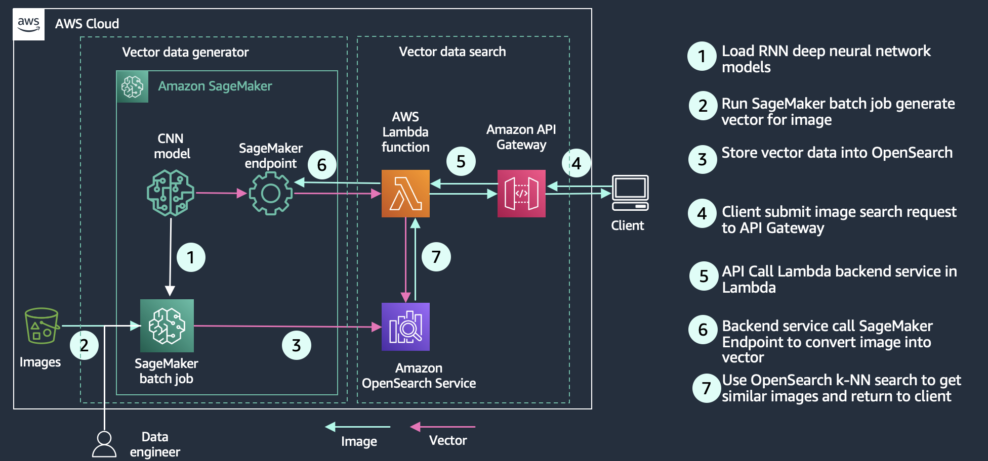
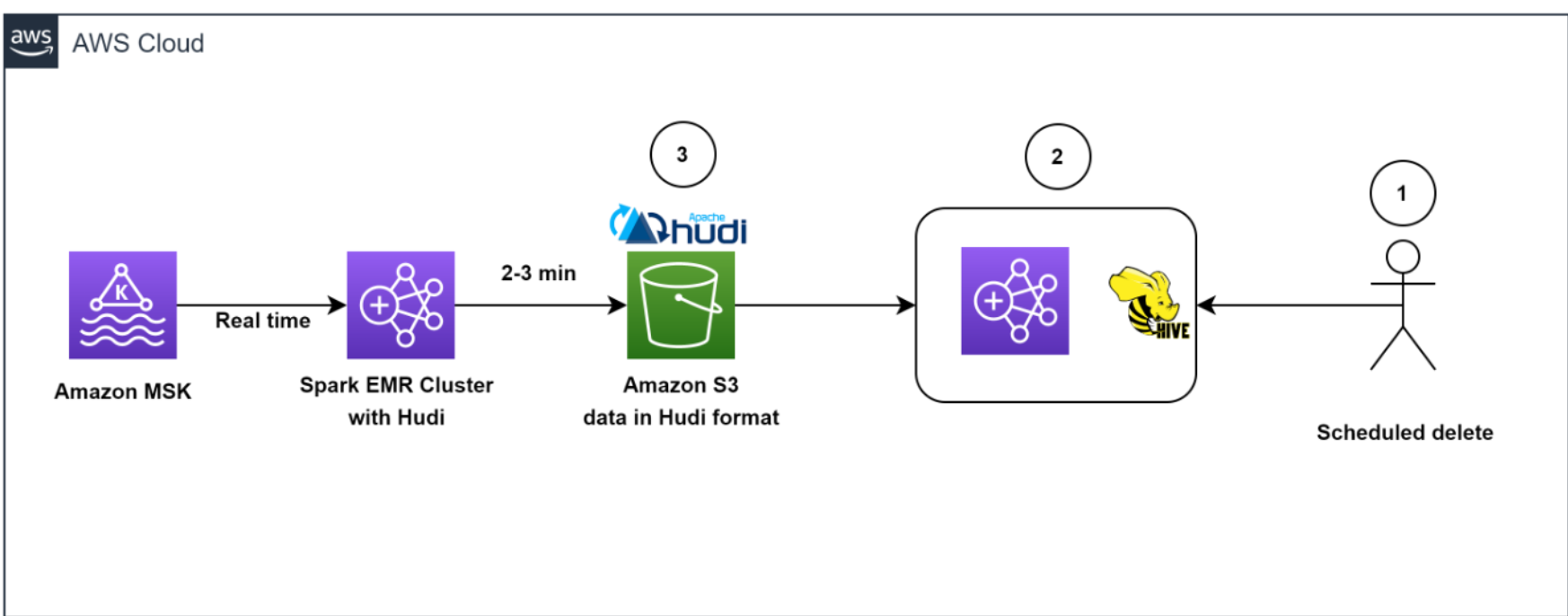
The high-level flow is the following:

  • Data is continuously updated from the data lake into either Redshift Serverless or the QuickSight caching layer, SPICE
  • An internal user can create an analysis and publish it as a dashboard for other internal or external users

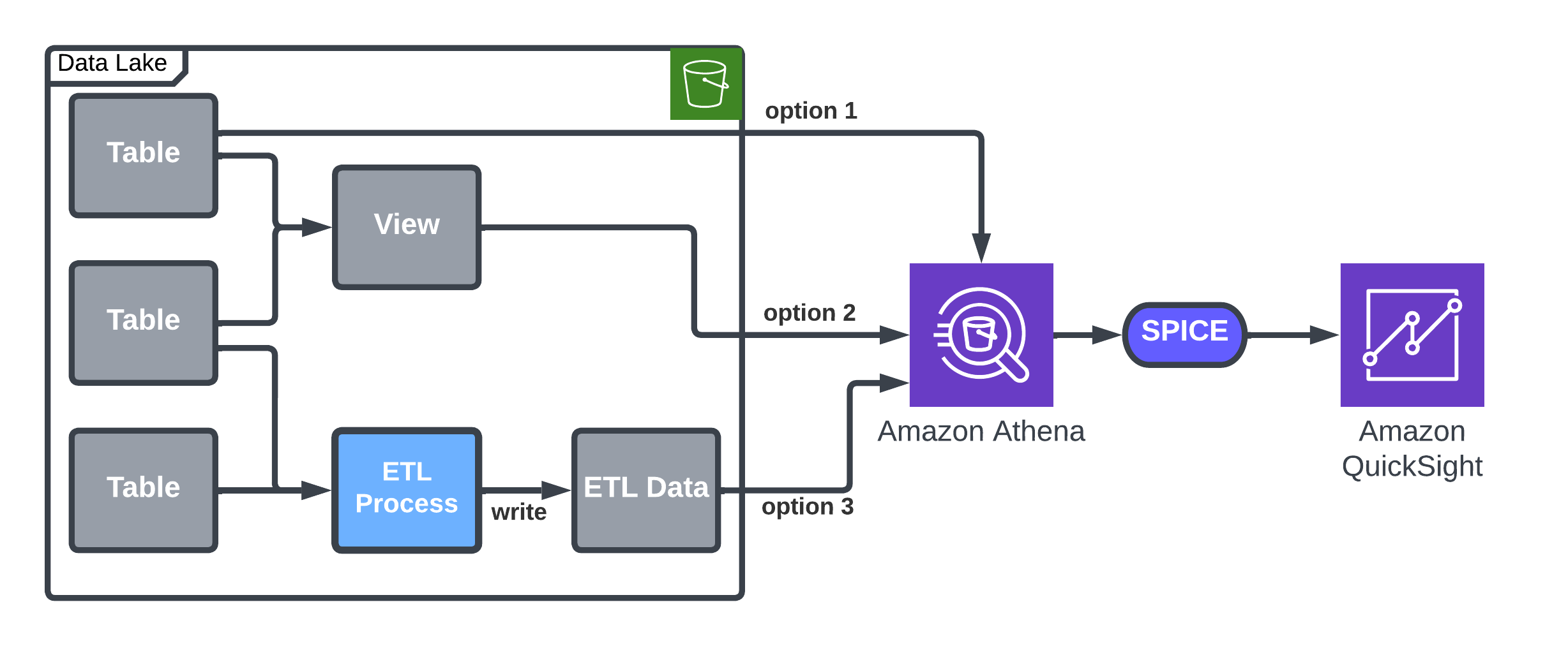
The following architecture diagram shows the high-level flow.

High-level flow

In the following sections, we discuss the details about the flow and the different solutions, including a comparison between them, which can help you choose the right solution for you.

Solution 1: Query with Athena and import to SPICE

QuickSight provides inherent capabilities to upload data using Athena into SPICE, which is a straightforward approach that meets Imperva’s requirements regarding simple data management. For example, it suits stable data flows without frequent exceptions, which may result in SPICE full refresh.

You can use Athena to load data into a QuickSight SPICE dataset, and then use the SPICE incremental upload option to load new data to the dataset. A QuickSight dataset will be connected to a table or a view accessible by Athena. A time column (like day or hour) is used for incremental updates. The following table summarizes the options and details.

Option Description Pros/Cons
Existing table Use the built-in option by QuickSight. Not flexible—the table is imported as is in the data lake.
Dedicated view

A view will let you better control the data in your dataset. It allows joining data, aggregation, or choosing a filter like the date you want to start importing data from.

Note that QuickSight allows building a dataset based on custom SQL, but this option doesn’t allow incremental updates.

Large Athena resource consumption on a full refresh.
Dedicated ETL

Create a dedicated ETL process, which is similar to a view, but unlike the view, it allows reuse of the results in case of a full refresh.

In case your ETL or view contains grouping or other complex operations, you know that these operations will be done only by the ETL process, according to the schedule you define.

Most flexible, but requires ETL development and implementation and additional Amazon S3 storage.

The following architecture diagram details the options for loading data by Athena into SPICE.

Architecture diagram details the options for loading data by Athena into SPICE

The following code provides a SQL example for a view creation. We assume the existence of two tables, customers and events, with one join column called customer_id. The view is used to do the following:

  • Aggregate the data from daily to weekly, and reduce the number of rows
  • Control the start date of the dataset (in this case, 30 weeks back)
  • Join the data to add more columns (customer_type) and filter it
CREATE VIEW my_dataset AS
SELECT DATE_ADD('day', -DAY_OF_WEEK(day) + 1, day) AS first_day_of_week,
       customer_type, event_type, COUNT(events) AS total_events
FROM my_events INNER JOIN my_customers USING (customer_id)
WHERE customer_type NOT IN ('Reseller')
      AND day BETWEEN DATE_ADD('DAY',-7 * 30 -DAY_OF_WEEK(CURRENT_DATE) + 1, CURRENT_DATE)
      AND DATE_ADD('DAY', -DAY_OF_WEEK(CURRENT_DATE), CURRENT_DATE)
GROUP BY 1, 2, 3

Solution 2: Load data into Redshift Serverless

Redshift Serverless provides full visibility to the data, which can be viewed or edited at any time. For example, if there is a delay in adding data to the data lake or the data isn’t properly added, with Redshift Serverless, you can edit data using SQL statements or retry data loading. Redshift Serverless is a scalable solution that doesn’t have a dataset size limitation.

Redshift Serverless is used as a serving layer for the datasets that are to be used in QuickSight. The pricing model for Redshift Serverless is based on storage utilization and the run of queries; idle compute resources have no associated cost. Setting up a cluster is simple and doesn’t require you to choose node types or amount of storage. You simply load the data to tables you create and start working.

To create a new dataset, you need to create an Amazon Redshift table and run the following process every time data is added:

  1. Transform the data using an ETL process (optional):
    • Read data from the tables.
    • Transform to the QuickSight dataset schema.
    • Write the data to an S3 bucket and load it to Amazon Redshift.
  2. Delete old data if it exists to avoid duplicate data.
  3. Load the data using the COPY command.

The following architecture diagram details the options to load data into Redshift Serverless with or without an ETL process.

Architecture diagram details the options to load data into Redshift Serverless with or without an ETL process

The Amazon Redshift COPY command is simple and fast. For example, to copy daily partition Parquet data, use the following code:

COPY my_table
FROM 's3://my_bucket/my_table/day=2022-01-01'
IAM_ROLE 'my_role' 
FORMAT AS PARQUET

Use the following COPY command to load the output file of the ETL process. Values will be truncated according to Amazon Redshift column size. The column truncation is important because, unlike in the data lake, in Amazon Redshift, the column size must be set. This option prevents COPY failures:

COPY my_table
FROM 's3://my_bucket/my_table/day=2022-01-01'
IAM_ROLE 'my_role' 
FORMAT AS JSON GZIP TRUNCATECOLUMNS

The Amazon Redshift COPY operation provides many benefits and options. It supports multiple formats as well as column mapping, escaping, and more. It also allows more control over data format, object size, and options to tune the COPY operation for improved performance. Unlike data in the data lake, Amazon Redshift has column length specifications. We use TRUNCATECOLUMNS to truncates the data in columns to the appropriate number of characters so that it fits the column specification.

Using this method provides full control over the data. In case of a problem, we can repair parts of the table by deleting old data and loading the data again. It’s also possible to use the QuickSight dataset JOIN option, which is not available in SPICE when using incremental update.

Additional benefit of this approach is that the data is available for other clients and services looking to use the same data, such as SQL clients or notebooks servers such as Apache Zeppelin.

Conclusion

QuickSight allows Imperva to expose business data to various departments within an organization. In the post, we explored approaches for importing data from a data lake to QuickSight, whether continuously or incrementally.

However, it’s important to note that there is no one-size-fits-all solution; the optimal approach will depend on the specific use case. Both options—continuous and incremental updates—are scalable and flexible, with no significant cost differences observed for our dataset and access patterns.

Imperva found incremental refresh to be very useful and uses it for simple data management. For more complex datasets, Imperva has benefitted from the greater scalability and flexibility provided by Redshift Serverless.

In cases where a higher degree of control over the datasets was required, Imperva chose Redshift Serverless so that data issues could be addressed promptly by deleting, updating, or inserting new records as necessary.

With the integration of dashboards, individuals can now access data that was previously inaccessible to them. Moreover, QuickSight has played a crucial role in streamlining our data distribution processes, enabling data accessibility across all departments within the organization.

To learn more, visit Amazon QuickSight.


About the Authors

Eliad Maimon is a Senior Startups Solutions Architect at AWS in Tel-Aviv with over 20 years of experience in architecting, building, and maintaining software products. He creates architectural best practices and collaborates with customers to leverage cloud and innovation, transforming businesses and disrupting markets. Eliad is specializing in machine learning on AWS, with a focus in areas such as generative AI, MLOps, and Amazon SageMaker.

Ori Nakar is a principal cyber-security researcher, a data engineer, and a data scientist at Imperva Threat Research group. Ori has many years of experience as a software engineer and engineering manager, focused on cloud technologies and big data infrastructure.

Amazon OpenSearch Service’s vector database capabilities explained

Post Syndicated from Jon Handler original https://aws.amazon.com/blogs/big-data/amazon-opensearch-services-vector-database-capabilities-explained/

OpenSearch is a scalable, flexible, and extensible open-source software suite for search, analytics, security monitoring, and observability applications, licensed under the Apache 2.0 license. It comprises a search engine, OpenSearch, which delivers low-latency search and aggregations, OpenSearch Dashboards, a visualization and dashboarding tool, and a suite of plugins that provide advanced capabilities like alerting, fine-grained access control, observability, security monitoring, and vector storage and processing. Amazon OpenSearch Service is a fully managed service that makes it simple to deploy, scale, and operate OpenSearch in the AWS Cloud.

As an end-user, when you use OpenSearch’s search capabilities, you generally have a goal in mind—something you want to accomplish. Along the way, you use OpenSearch to gather information in support of achieving that goal (or maybe the information is the original goal). We’ve all become used to the “search box” interface, where you type some words, and the search engine brings back results based on word-to-word matching. Let’s say you want to buy a couch in order to spend cozy evenings with your family around the fire. You go to Amazon.com, and you type “a cozy place to sit by the fire.” Unfortunately, if you run that search on Amazon.com, you get items like fire pits, heating fans, and home decorations—not what you intended. The problem is that couch manufacturers probably didn’t use the words “cozy,” “place,” “sit,” and “fire” in their product titles or descriptions.

In recent years, machine learning (ML) techniques have become increasingly popular to enhance search. Among them are the use of embedding models, a type of model that can encode a large body of data into an n-dimensional space where each entity is encoded into a vector, a data point in that space, and organized such that similar entities are closer together. An embedding model, for instance, could encode the semantics of a corpus. By searching for the vectors nearest to an encoded document — k-nearest neighbor (k-NN) search — you can find the most semantically similar documents. Sophisticated embedding models can support multiple modalities, for instance, encoding the image and text of a product catalog and enabling similarity matching on both modalities.

A vector database provides efficient vector similarity search by providing specialized indexes like k-NN indexes. It also provides other database functionality like managing vector data alongside other data types, workload management, access control and more. OpenSearch’s k-NN plugin provides core vector database functionality for OpenSearch, so when your customer searches for “a cozy place to sit by the fire” in your catalog, you can encode that prompt and use OpenSearch to perform a nearest neighbor query to surface that 8-foot, blue couch with designer arranged photographs in front of fireplaces.

Using OpenSearch Service as a vector database

With OpenSearch Service’s vector database capabilities, you can implement semantic search, Retrieval Augmented Generation (RAG) with LLMs, recommendation engines, and search rich media.

Semantic search

With semantic search, you improve the relevance of retrieved results using language-based embeddings on search documents. You enable your search customers to use natural language queries, like “a cozy place to sit by the fire” to find their 8-foot-long blue couch. For more information, refer to Building a semantic search engine in OpenSearch to learn how semantic search can deliver a 15% relevance improvement, as measured by normalized discounted cumulative gain (nDCG) metrics compared with keyword search. For a concrete example, our Improve search relevance with ML in Amazon OpenSearch Service workshop explores the difference between keyword and semantic search, based on a Bidirectional Encoder Representations from Transformers (BERT) model, hosted by Amazon SageMaker to generate vectors and store them in OpenSearch. The workshop uses product question answers as an example to show how keyword search using the keywords/phrases of the query leads to some irrelevant results. Semantic search is able to retrieve more relevant documents by matching the context and semantics of the query. The following diagram shows an example architecture for a semantic search application with OpenSearch Service as the vector database.

Architecture diagram showing how to use Amazon OpenSearch Service to perform semantic search to improve relevance

Retrieval Augmented Generation with LLMs

RAG is a method for building trustworthy generative AI chatbots using generative LLMs like OpenAI, ChatGPT, or Amazon Titan Text. With the rise of generative LLMs, application developers are looking for ways to take advantage of this innovative technology. One popular use case involves delivering conversational experiences through intelligent agents. Perhaps you’re a software provider with knowledge bases for product information, customer self-service, or industry domain knowledge like tax reporting rules or medical information about diseases and treatments. A conversational search experience provides an intuitive interface for users to sift through information through dialog and Q&A. Generative LLMs on their own are prone to hallucinations—a situation where the model generates a believable but factually incorrect response. RAG solves this problem by complementing generative LLMs with an external knowledge base that is typically built using a vector database hydrated with vector-encoded knowledge articles.

As illustrated in the following diagram, the query workflow starts with a question that is encoded and used to retrieve relevant knowledge articles from the vector database. Those results are sent to the generative LLM whose job is to augment those results, typically by summarizing the results as a conversational response. By complementing the generative model with a knowledge base, RAG grounds the model on facts to minimize hallucinations. You can learn more about building a RAG solution in the Retrieval Augmented Generation module of our semantic search workshop.

Architecture diagram showing how to use Amazon OpenSearch Service to perform retrieval-augmented generation

Recommendation engine

Recommendations are a common component in the search experience, especially for ecommerce applications. Adding a user experience feature like “more like this” or “customers who bought this also bought that” can drive additional revenue through getting customers what they want. Search architects employ many techniques and technologies to build recommendations, including Deep Neural Network (DNN) based recommendation algorithms such as the two-tower neural net model, YoutubeDNN. A trained embedding model encodes products, for example, into an embedding space where products that are frequently bought together are considered more similar, and therefore are represented as data points that are closer together in the embedding space. Another possibility
is that product embeddings are based on co-rating similarity instead of purchase activity. You can employ this affinity data through calculating the vector similarity between a particular user’s embedding and vectors in the database to return recommended items. The following diagram shows an example architecture of building a recommendation engine with OpenSearch as a vector store.

Architecture diagram showing how to use Amazon OpenSearch Service as a recommendation engine

Media search

Media search enables users to query the search engine with rich media like images, audio, and video. Its implementation is similar to semantic search—you create vector embeddings for your search documents and then query OpenSearch Service with a vector. The difference is you use a computer vision deep neural network (e.g. Convolutional Neural Network (CNN)) such as ResNet to convert images into vectors. The following diagram shows an example architecture of building an image search with OpenSearch as the vector store.

Architecture diagram showing how to use Amazon OpenSearch Service to search rich media like images, videos, and audio files

Understanding the technology

OpenSearch uses approximate nearest neighbor (ANN) algorithms from the NMSLIB, FAISS, and Lucene libraries to power k-NN search. These search methods employ ANN to improve search latency for large datasets. Of the three search methods the k-NN plugin provides, this method offers the best search scalability for large datasets. The engine details are as follows:

  • Non-Metric Space Library (NMSLIB) – NMSLIB implements the HNSW ANN algorithm
  • Facebook AI Similarity Search (FAISS) – FAISS implements both HNSW and IVF ANN algorithms
  • Lucene – Lucene implements the HNSW algorithm

Each of the three engines used for approximate k-NN search has its own attributes that make one more sensible to use than the others in a given situation. You can follow the general information in this section to help determine which engine will best meet your requirements.

In general, NMSLIB and FAISS should be selected for large-scale use cases. Lucene is a good option for smaller deployments, but offers benefits like smart filtering where the optimal filtering strategy—pre-filtering, post-filtering, or exact k-NN—is automatically applied depending on the situation. The following table summarizes the differences between each option.

.

NMSLIB-HNSW

FAISS-HNSW

FAISS-IVF

Lucene-HNSW

Max Dimension

16,000

16,000

16,000

1024

Filter

Post filter

Post filter

Post filter

Filter while search

Training Required

No

No

Yes

No

Similarity Metrics

l2, innerproduct, cosinesimil, l1, linf

l2, innerproduct

l2, innerproduct

l2, cosinesimil

Vector Volume

Tens of billions

Tens of billions

Tens of billions

< Ten million

Indexing latency

Low

Low

Lowest

Low

Query Latency & Quality

Low latency & high quality

Low latency & high quality

Low latency & low quality

High latency & high quality

Vector Compression

Flat

Flat

Product Quantization

Flat

Product Quantization

Flat

Memory Consumption

High

High

Low with PQ

Medium

Low with PQ

High

Approximate and exact nearest-neighbor search

The OpenSearch Service k-NN plugin supports three different methods for obtaining the k-nearest neighbors from an index of vectors: approximate k-NN, score script (exact k-NN), and painless extensions (exact k-NN).

Approximate k-NN

The first method takes an approximate nearest neighbor approach—it uses one of several algorithms to return the approximate k-nearest neighbors to a query vector. Usually, these algorithms sacrifice indexing speed and search accuracy in return for performance benefits such as lower latency, smaller memory footprints, and more scalable search. Approximate k-NN is the best choice for searches over large indexes (that is, hundreds of thousands of vectors or more) that require low latency. You should not use approximate k-NN if you want to apply a filter on the index before the k-NN search, which greatly reduces the number of vectors to be searched. In this case, you should use either the score script method or painless extensions.

Score script

The second method extends the OpenSearch Service score script functionality to run a brute force, exact k-NN search over knn_vector fields or fields that can represent binary objects. With this approach, you can run k-NN search on a subset of vectors in your index (sometimes referred to as a pre-filter search). This approach is preferred for searches over smaller bodies of documents or when a pre-filter is needed. Using this approach on large indexes may lead to high latencies.

Painless extensions

The third method adds the distance functions as painless extensions that you can use in more complex combinations. Similar to the k-NN score script, you can use this method to perform a brute force, exact k-NN search across an index, which also supports pre-filtering. This approach has slightly slower query performance compared to the k-NN score script. If your use case requires more customization over the final score, you should use this approach over score script k-NN.

Vector search algorithms

The simple way to find similar vectors is to use k-nearest neighbors (k-NN) algorithms, which compute the distance between a query vector and the other vectors in the vector database. As we mentioned earlier, the score script k-NN and painless extensions search methods use the exact k-NN algorithms under the hood. However, in the case of extremely large datasets with high dimensionality, this creates a scaling problem that reduces the efficiency of the search. Approximate nearest neighbor (ANN) search methods can overcome this by employing tools that restructure indexes more efficiently and reduce the dimensionality of searchable vectors. There are different ANN search algorithms; for example, locality sensitive hashing, tree-based, cluster-based, and graph-based. OpenSearch implements two ANN algorithms: Hierarchical Navigable Small Worlds (HNSW) and Inverted File System (IVF). For a more detailed explanation of how the HNSW and IVF algorithms work in OpenSearch, see blog post “Choose the k-NN algorithm for your billion-scale use case with OpenSearch”.

Hierarchical Navigable Small Worlds

The HNSW algorithm is one of the most popular algorithms out there for ANN search. The core idea of the algorithm is to build a graph with edges connecting index vectors that are close to each other. Then, on search, this graph is partially traversed to find the approximate nearest neighbors to the query vector. To steer the traversal towards the query’s nearest neighbors, the algorithm always visits the closest candidate to the query vector next.

Inverted File

The IVF algorithm separates your index vectors into a set of buckets, then, to reduce your search time, only searches through a subset of these buckets. However, if the algorithm just randomly split up your vectors into different buckets, and only searched a subset of them, it would yield a poor approximation. The IVF algorithm uses a more elegant approach. First, before indexing begins, it assigns each bucket a representative vector. When a vector is indexed, it gets added to the bucket that has the closest representative vector. This way, vectors that are closer to each other are placed roughly in the same or nearby buckets.

Vector similarity metrics

All search engines use a similarity metric to rank and sort results and bring the most relevant results to the top. When you use a plain text query, the similarity metric is called TF-IDF, which measures the importance of the terms in the query and generates a score based on the number of textual matches. When your query includes a vector, the similarity metrics are spatial in nature, taking advantage of proximity in the vector space. OpenSearch supports several similarity or distance measures:

  • Euclidean distance – The straight-line distance between points.
  • L1 (Manhattan) distance – The sum of the differences of all of the vector components. L1 distance measures how many orthogonal city blocks you need to traverse from point A to point B.
  • L-infinity (chessboard) distance – The number of moves a King would make on an n-dimensional chessboard. It’s different than Euclidean distance on the diagonals—a diagonal step on a 2-dimensional chessboard is 1.41 Euclidean units away, but 2 L-infinity units away.
  • Inner product – The product of the magnitudes of two vectors and the cosine of the angle between them. Usually used for natural language processing (NLP) vector similarity.
  • Cosine similarity – The cosine of the angle between two vectors in a vector space.
  • Hamming distance – For binary-coded vectors, the number of bits that differ between the two vectors.

Advantage of OpenSearch as a vector database

When you use OpenSearch Service as a vector database, you can take advantage of the service’s features like usability, scalability, availability, interoperability, and security. More importantly, you can use OpenSearch’s search features to enhance the search experience. For example, you can use Learning to Rank in OpenSearch to integrate user clickthrough behavior data into your search application and improve search relevance. You can also combine OpenSearch text search and vector search capabilities to search documents with keyword and semantic similarity. You can also use other fields in the index to filter documents to improve relevance. For advanced users, you can use a hybrid scoring model to combine OpenSearch’s text-based relevance score, computed with the Okapi BM25 function and its vector search score to improve the ranking of your search results.

Scale and limits

OpenSearch as vector database support billions of vector records. Keep in mind the following calculator regarding number of vectors and dimensions to size your cluster.

Number of vectors

OpenSearch VectorDB takes advantage of the sharding capabilities of OpenSearch and can scale to billions of vectors at single-digit millisecond latencies by sharding vectors and scale horizontally by adding more nodes. The number of vectors that can fit in a single machine is a function of the off-heap memory availability on the machine. The number of nodes required will depend on the amount of memory that can be used for the algorithm per node and the total amount of memory required by the algorithm. The more nodes, the more memory and better performance. The amount of memory available per node is computed as memory_available = (node_memoryjvm_size) * circuit_breaker_limit, with the following parameters:

  • node_memory – The total memory of the instance.
  • jvm_size – The OpenSearch JVM heap size. This is set to half of the instance’s RAM, capped at approximately 32 GB.
  • circuit_breaker_limit – The native memory usage threshold for the circuit breaker. This is set to 0.5.

Total cluster memory estimation depends on total number of vector records and algorithms. HNSW and IVF have different memory requirements. You can refer to Memory Estimation for more details.

Number of dimensions

OpenSearch’s current dimension limit for the vector field knn_vector is 16,000 dimensions. Each dimension is represented as a 32-bit float. The more dimensions, the more memory you’ll need to index and search. The number of dimensions is usually determined by the embedding models that translate the entity to a vector. There are a lot of options to choose from when building your knn_vector field. To determine the correct methods and parameters to choose, refer to Choosing the right method.

Customer stories:

Amazon Music

Amazon Music is always innovating to provide customers with unique and personalized experiences. One of Amazon Music’s approaches to music recommendations is a remix of a classic Amazon innovation, item-to-item collaborative filtering, and vector databases. Using data aggregated based on user listening behavior, Amazon Music has created an embedding model that encodes music tracks and customer representations into a vector space where neighboring vectors represent tracks that are similar. 100 million songs are encoded into vectors, indexed into OpenSearch, and served across multiple geographies to power real-time recommendations. OpenSearch currently manages 1.05 billion vectors and supports a peak load of 7,100 vector queries per second to power Amazon Music recommendations.

The item-to-item collaborative filter continues to be among the most popular methods for online product recommendations because of its effectiveness at scaling to large customer bases and product catalogs. OpenSearch makes it easier to operationalize and further the scalability of the recommender by providing scale-out infrastructure and k-NN indexes that grow linearly with respect to the number of tracks and similarity search in logarithmic time.

The following figure visualizes the high-dimensional space created by the vector embedding.

A visualization of the vector encoding of Amazon Music entries in the large vector space

Brand protection at Amazon

Amazon strives to deliver the world’s most trustworthy shopping experience, offering customers the widest possible selection of authentic products. To earn and maintain our customers’ trust, we strictly prohibit the sale of counterfeit products, and we continue to invest in innovations that ensure only authentic products reach our customers. Amazon’s brand protection programs build trust with brands by accurately representing and completely protecting their brand. We strive to ensure that public perception mirrors the trustworthy experience we deliver. Our brand protection strategy focuses on four pillars: (1) Proactive Controls (2) Powerful Tools to Protect Brands (3) Holding Bad Actors Accountable (4) Protecting and Educating Customers. Amazon OpenSearch Service is a key part of Amazon’s Proactive Controls.

In 2022, Amazon’s automated technology scanned more than 8 billion attempted changes daily to product detail pages for signs of potential abuse. Our proactive controls found more than 99% of blocked or removed listings before a brand ever had to find and report it. These listings were suspected of being fraudulent, infringing, counterfeit, or at risk of other forms of abuse. To perform these scans, Amazon created tooling that uses advanced and innovative techniques, including the use of advanced machine learning models to automate the detection of intellectual property infringements in listings across Amazon’s stores globally. A key technical challenge in implementing such automated system is the ability to search for protected intellectual property within a vast billion-vector corpus in a fast, scalable and cost effective manner. Leveraging Amazon OpenSearch Service’s scalable vector database capabilities and distributed architecture, we successfully developed an ingestion pipeline that has indexed a total of 68 billion, 128- and 1024-dimension vectors into OpenSearch Service to enable brands and automated systems to conduct infringement detection, in real-time, through a highly available and fast (sub-second) search API.

Conclusion

Whether you’re building a generative AI solution, searching rich media and audio, or bringing more semantic search to your existing search-based application, OpenSearch is a capable vector database. OpenSearch supports a variety of engines, algorithms, and distance measures that you can employ to build the right solution. OpenSearch provides a scalable engine that can support vector search at low latency and up to billions of vectors. With OpenSearch and its vector DB capabilities, your users can find that 8-foot-blue couch easily, and relax by a cozy fire.


About the Authors

Jon Handler is a Senior Principal Solutions Architect with AWSJon Handler is a Senior Principal Solutions Architect at Amazon Web Services based in Palo Alto, CA. Jon works closely with OpenSearch and Amazon OpenSearch Service, providing help and guidance to a broad range of customers who have search and log analytics workloads that they want to move to the AWS Cloud. Prior to joining AWS, Jon’s career as a software developer included four years of coding a large-scale, eCommerce search engine. Jon holds a Bachelor of the Arts from the University of Pennsylvania, and a Master of Science and a Ph. D. in Computer Science and Artificial Intelligence from Northwestern University.

Jianwei Li is a Principal Analytics Specialist TAM at Amazon Web Services. Jianwei provides consultant service for customers to help customer design and build modern data platform. Jianwei has been working in big data domain as software developer, consultant and tech leader.

Dylan Tong is a Senior Product Manager at AWS. He works with customers to help drive their success on the AWS platform through thought leadership and guidance on designing well architected solutions. He has spent most of his career building on his expertise in data management and analytics by working for leaders and innovators in the space.

Vamshi Vijay Nakkirtha is a Software Engineering Manager working on the OpenSearch Project and Amazon OpenSearch Service. His primary interests include distributed systems. He is an active contributor to various plugins, like k-NN, GeoSpatial, and dashboard-maps.

How GoDaddy Implemented a Multi-Region Event-Driven Platform at Scale

Post Syndicated from Marcia Villalba original https://aws.amazon.com/blogs/aws/how-godaddy-implemented-a-multi-region-event-driven-platform-at-scale/

GoDaddy, a leading global provider of domain registration and web hosting services, has served over 84 million domains and 22 million customers since its establishment in 1997. Among its various internal systems, the Customer Signal Platform provides tooling to capture, analyze, and act on customer and product data to drive better business outcomes. With this platform, GoDaddy can track user visits and interactions on its website and use meaningful event data to improve its customer experience and overall business performance.

Nowadays, the Customer Signal Platform processes 400 million events every day. As GoDaddy expands its integrations, it aims to increase this number to 2 billion events per day in the near future.

When building the Customer Signal Platform, GoDaddy had three main requirements for the system architecture:

  1. Minimize their operational load.
  2. Scale automatically as traffic changes.
  3. Provide high availability and ensure that all the customer signals are captured.

Amazon EventBridge Event Bus
After evaluating many options against their requirements, GoDaddy decided to implement the customer signal platform using Amazon EventBridge Event Bus. EventBridge Event Bus is a serverless event bus that helps you receive, filter, transform, route, and deliver events. Because EventBridge is serverless, it requires minimal configuration to get started and scales automatically—GoDaddy’s first two requirements were checked.

To comply with the third requirement, the solution needed to provide business continuity and ensure that no event is lost from the moment the client produces it until it gets to the platform to be analyzed. EventBridge Event Bus comes with many features that helped GoDaddy build their application with this requirement in mind.

The main feature that GoDaddy took advantage of was global endpoints. EventBridge global endpoints provide a reliable and simple way to improve the business continuity of event-driven applications. This new feature, added in 2022, allows customers to build a multi-Region event-driven application.

EventBridge Global Endpoints
Global endpoints allow you to configure a managed DNS endpoint in EventBridge, to which your applications will send events. Then you need to configure two custom event buses in two distinct AWS Regions. One is the primary Region, and the other is the failover, or secondary Region. The failover of events is decided based on the health indicated by an Amazon Route 53 health check. When the health check is healthy, the events are routed from the global endpoint to the custom event bus in the primary Region. And if the health check is unhealthy, then the global endpoint will send the events to the event bus in the secondary Region.

Healthcheck status

The simplest configuration for global endpoints is the active/archive configuration. This configuration provides business continuity and simplicity at the same time. The active/archive configuration defines two different Regions. The primary Region is where the application is deployed and all the business processes are happening. The archive Region is where only a custom bus is deployed and all the events are archived.

In addition, there is a bidirectional replication rule between the buses in separate Regions. In the normal case, when there are no errors, whenever an event arrives at the custom bus in the primary Region, the event is automatically replicated to the archive custom bus in the secondary Region.

In the case of failover, the global endpoint redirects the events to the secondary Region, where they get archived for processing at another time.

Active/ Archive configuration

GoDaddy Implementation of Global Endpoints
GoDaddy was looking for a solution that minimized their operations load while still providing business continuity, and that is why they adopted global endpoints and the active/archive configuration. In this way, they could have the event processing logic in their primary Region and have a secondary Region in case of any issues.

In their configuration, events are archived in the secondary Region for 30 days, after which the events expire. In the case of a failover, because they don’t need to process the events in real time, they collect them in the archive. If the issue is resolved within 24 hours, the retention period for the replication rule, the events are sent automatically to the primary Region. If the issue is solved in more than 24 hours the events need to be replayed to the primary Region.

The following image shows what their current solution looks like. They are working with two Regions. US West (Oregon) is their primary Region and is the location of the data lake, which is the primary consumer of the events. US East (N. Virginia) is the secondary Region. Events are being produced in different clients; from the clients, they are sent to Amazon API Gateway. GoDaddy deployed two API Gateways in their two Regions. The events are sent to the API Gateway with the smallest latency from the client. To do that, they use latency-based routing provided by Amazon Route 53. Then events are sent to an AWS Lambda function that validates the events and forwards them to the EventBridge global endpoint at the DNS level.

GoDaddy architecture

The global endpoint is configured with the active/archive setup, and the failover is configured to be triggered via a Route 53 health check that monitors an Amazon CloudWatch alarm. That alarm observes the IngestionToInvocationStartLatency metric in the primary Region.

IngestionToInvocationStartLatency is a service-level metric that exposes the time to process events from the point at which they are ingested by EventBridge to the point the first invocation of a target in the configured rules is made. This metric is measured across all the rules in your bus and provides an indication of the health of the EventBridge service. Any extended periods of high latency over 30 seconds indicate a service disruption.

When the system is in the normal state, the events are forwarded from the global endpoint to the custom ingress event bus in the primary Region. That custom event bus has replication enabled; this means that all the events that arrive at the bus get replicated automatically in the secondary Region custom ingress event bus.

All the events received by the ingress event bus are sent to the enrichment function. This function performs basic validation and authentication, and it enriches the event data to make sure that all the events from different clients are standard.

From there, the events are forwarded to the data platform event bus to be sent to the different consumer targets. The main target is their data lake solution, which analyzes all the events.

What Was the Impact?
For GoDaddy, business continuity is important, and their customer signals are not getting lost due to any issue with their platform. This makes them confident that they can expand their customer signal platforms from 400 million events per day to 2 billion events per day without introducing any additional operations overhead.

Now, they can confidently process hundreds of millions of events per day to their system, and they can keep on growing. The following image shows the number of events ingested by global endpoints in a normal day.

Events ingested

While GoDaddy’s use of the active/archive pattern enables them to ensure they never lose any events, they’re already starting to see certain use cases where they want to minimize any delays in processing their events, even when service disruptions occur. Because they’re already replicating their events to a secondary Region, they can deploy their most critical consumers to both Regions and enable an active/active configuration for their mission-critical systems. Active/active configuration allows you to process parallel events in both the primary and secondary Regions, simplifying the processing of events even during disruptions and enabling business continuity.

The vision when building the Customer Signal Platform was to align with GoDaddy’s high bar for reliability, scalability, and maintainability and, at the same time, keep the platform self-service so that developers can focus on business needs. This led GoDaddy to choose Amazon EventBridge global endpoints and serverless technologies to build this solution.

GoDaddy Customer Signal Platform is an excellent example of what serverless technologies enable. By leveraging the cloud to handle as much of the undifferentiated heavy lifting as possible, GoDaddy has reduced the operational complexity of setting up an event bus for a multi-Region strategy, implemented failover mechanisms in the case of Regional distruptions, and ensured that events are not lost by enabling replication. Global endpoints active/archive configuration improves the availability of customer applications with the least amount of configuration changes.

If you want to get started with EventBridge global endpoints, you can check out this talk on event-driven applications. For a working demo on how to use EventBridge global endpoints for failover events, check out this Serverless Land repository.

Marcia

Deploying an automated Amazon CloudWatch dashboard for AWS Outposts using AWS CDK

Post Syndicated from Sheila Busser original https://aws.amazon.com/blogs/compute/deploying-an-automated-amazon-cloudwatch-dashboard-for-aws-outposts-using-aws-cdk/

This post is written by Enrico Liguori, Networking Solutions Architect, Hybrid Cloud and Sumeeth Siriyur, Sr. Hybrid Cloud Solutions Architect.

AWS Outposts is a fully managed service that brings the same AWS infrastructure, services, APIs, and tools to virtually any data center, colocation space, manufacturing floor, or on-premises facility where it might be needed. With Outposts, you can run some AWS services on-premises and connect to a broad range of services available in the local AWS Region. Outposts supports workloads requiring low latency, local data processing, data residency, and application migration.

Outposts capacity is driven as per your compute and storage requirements to run workloads. You can monitor Outposts resources using metrics gathered by Amazon CloudWatch. Using these metrics, you can effectively monitor and manage the Outposts resources as they would in the Region, levereging cloud native tools such as CloudWatch dashboards. Check the Monitoring best practices for AWS Outposts blog post to dive deep into the available monitoring options for Outposts.

CloudWatch dashboards are customizable home pages in the CloudWatch console that can be used to monitor resources running on Outposts in a single view. For example, you can monitor in a single pane the number Amazon EC2 instances used per EC2 instance type, the available capacity of Amazon EBS volumes and Amazon S3 buckets, and the operational status of the service link of Outposts.

As a you start deploying additional Outposts resources as a part of their capacity expansion, they must all be integrated and visualized within CloudWatch in an automated way. Traditionally CloudWatch dashboards are built manually and may be time consuming to tune. This post provides also an overview of building CloudWatch dashboards in an automated way using AWS Cloud Development Kit (AWS CDK).

Overview

CloudWatch metrics available to monitor Outposts resources and capacity

CloudWatch metrics for Outposts are available to customers in all public AWS Regions and AWS GovCloud (US) at no additional cost. We can classify the available metrics in two main categories:

To identify the metrics published under the service specific namespaces, we can leverage metadata in the form of tags. A tag is a label that you assign to an AWS resource and consists of a key and an optional value. For the purpose of the monitoring strategy described in this post, we use a tag that contains the OutpostID of the Outpost where the resource is deployed. In this way, we can easily filter the CloudWatch metrics that we would like to show in our dashboard.

To enforce the assignment of tags to our resources we can implement a tagging strategy using AWS tag Policies and Service Control Policies (SCPs).

The following sections describe two different methods to build a CloudWatch dashboard that includes the different types of metrics described so far. In both cases, we see how particularly useful the presence of tags is to identify the service-specific metrics.

Manual approach to building a CloudWatch dashboard for Outposts

This section describes a manual (i.e., non-automated) approach to building a dashboard that could summarize both the capacity utilization metrics and the service specific metrics for your resources running on Outposts.

The benefit of this approach is that we can implement a fully operational dashboard directly from the CloudWatch console. However, it will simultaneously require more effort to properly tune the dashboard to satisfy your monitoring requirements.

You can start creating the dashboard opening the CloudWatch console and following the steps listed in the public documentation.

To display a metric under AWS/Outposts namespace we can choose any of the widgets available. Based on the nature of the data, we can choose different types of Widgets such as Number, Line, Gauge, Explorer, or you can even build your own custom widget.

Together with the Widget type, we must select Outposts namespace in the metric graph dialog box and then navigate to the specific metric of interest.

In case we are creating the dashboard in a different account than the Outposts owner, we must select the right account in the View data drop-down menu to see the Outposts metric in which we are interested.

View data drop-down menu

After selecting one or more metrics we can select Create widget button.

For the service specific metrics, we recommend using the explorer widget. In this way, we can utilize the tagging strategy described earlier to automatically identify the metrics belonging to the resources running on Outposts. Check the documentation page for a step-by-step guide for creating an explorer widget based on tags.

Automated outpost dashboard

After we’ve seen how to build a dashboard manually from the console, in this secton we describe an automated approach to deploy a dashboard for Outposts through AWS CDK.

AWS CDK is an open source software development framework to model and provision your cloud application resources using familiar programming languages, including TypeScript, JavaScript, Python, C#, and Java. For the solution in this post, we use Python.

Architecture overview

The AWS CDK stack described in this post, assumes that the resources running on Outposts (EC2 instances, S3 buckets, Application Load Balancers (ALBs), and RDS instances) are tagged using the tagging strategy described earlier.

Specifying a tag name and a tag value in a configuration file automatically discovers the resources with that tag and adds the related metrics to the CloudWatch dashboard.

Together with the service specific metrics, it creates a series of widgets that we can use to monitor the capacity available and utilized in each Outpost that belongs to the account where the script is running.

The workflow is made of the following phases:

  1. The AWS CDK stack creates an AWS CodeCommit repository and uploads its own code into it. The code contains a series of modules, one for each section of the CloudWatch dashboard. A section of the dashboard contains one or more widgets showing the metrics of a specific service.
  2. To maintain the CloudWatch dashboard always up-to-date with the resources matching the tag, it creates a pipeline in AWS CodePipeline that can dynamically create and or update the dashboard. The pipeline runs the code in the CodeCommit repository and is made of two stages. In the first one, the build stage, it builds the dependencies needed by the AWS CDK stack. In the second stage, the Deploy stage, it loads and runs the modules used to build the dashboard.
  3. Each module contains the code to automatically discover the tagged resources of a specific service. This discovery phase uses standard AWS APIs called through the Python SDK Boto3.
  4. Based on the results of the discovery phase, AWS CDK produces an AWS CloudFormation template containing the definition of the CloudWatch dashboard sections. The template is submitted to CloudFormation.
  5. CloudFormation creates or, if already defined, updates the CloudWatch dashboard.
  6. Together with the dashboard, the AWS CDK script also contains the definition of a CloudWatch Event that, once deployed, triggers the pipeline each time a resource tagged with the specified tag is created or destroyed.

Prerequisites

To implement the solution presented in this post, you must configure:

  1. git as distributed version control system.
  2. In case it is the first time that you’re using AWS CDK in this account and region, you must:

a. Install the AWS CDK, and its prerequisites, following these instructions.

b. Go through the AWS CDK bootstrapping process. This is required only for the first time that we use AWS CDK in a specific AWS environment (an AWS environment is a combination of an AWS account and Region).

How to install

Step 1: Clone the AWS CDK code hosted on GitHub with:

$ git clone https://github.com/aws-samples/automated-cloudwatch-dashboard.git

Step 2: enter the directory using the following:

$ cd  automated-cloudwatch-dashboard/

Step 3: Install the needed Python dependencies with:

$ pip install -r requirements.txt

Step 4: Modify the configuration file

Before deploying the stack, we must modify the configuration file to specify the tag we use for identifying our resources running on Outposts. Open the file with the name config.yaml with your preferred text editor and specify:

      • A name for the dashboard. The default name used is Automated-CloudWatch-Dashboard.
      • Replace <tag_name> placeholder following the tag_name variable with the tag name used to tag the resources that you want to include in the dashboard.
      • Replace <tag_value> placeholder under tag_values variable with the tag value that you used.

Here is an example config.yaml configuration file:

dashboard_name: Automated-CloudWatch-Dahsboard
tag_name: OutpostID
tag_values:
  - op-1234567890abcdefg 

Stack deployment

We can deploy the stack with the following:

$ cdk deploy

At the end of the deployment process, the pipeline that creates the dashboard is provisioned. You can now go to your CloudWatch console to view it.

Automated Outposts dashboard overview

Now that we have built our dashboard, let’s review each section:

  1. Outpost capacity

Outpost Capacity diagram

The AWS CDK stacks define a capacity section for each Outpost available to the AWS account where the script runs.

In this section, we find four widgets showing metrics published under the AWS/Outpost namespace. The first widget shows for each EC2 instance type available on the Outposts the number of instances utilized and available for that instance type. In the second row, we can visualize the available capacity for the Amazon EBS volumes and for the S3 buckets. The last widget shows the operational status of the service link of Outposts.

2. EC2 instances

CPU, Network, and Disk Utilization for an EC2 instance diagram

In this section of the dashboard, we find the metrics showing the CPU, Network, and Disk Utilization for an EC2 instance. It has defined a section of this type for each EC2 instance with a tag assigned matching the name and the value specified in the configuration file of the script.

3. Application Load Balancer

The ALB section aggregates metrics showing the operational status of a load balancer hosted on Outposts

The ALB section aggregates metrics showing the operational status of a load balancer hosted on Outposts. A section of this type is defined for each ALB with an assigned tag matching the one specified in the configuration file.

4. S3 buckets

The S3 buckets section diagram

The S3 buckets section is defined only once and aggregates the utilization metrics for all S3 buckets with an assigned tag.

5. AutoScaling group

The AutoScaling group section diagram

The AutoScaling group section can be used to monitor the number of instances in service in a specific AS group with a tag assigned. This section is defined once and can aggregate the metrics for multiple AutoScaling groups.

Clean up

To terminate the resources that we created in this post, run the following:

$ cdk destroy

Then, go to the Cloudformation console and delete the stack with the name “Deploy-AutomatedCloudWatchDashboard”.

Conclusion

In conclusion, this post demonstrates a manual way of creating CloudWatch Metrics dashboard using the CloudWatch console and an automated way using AWS CDK. The automated approach is also scalable by automatically discovering any new resources added to the existing Outposts in the your environment without any changes to the code.

Secure Connectivity from Public to Private: Introducing EC2 Instance Connect Endpoint

Post Syndicated from Sheila Busser original https://aws.amazon.com/blogs/compute/secure-connectivity-from-public-to-private-introducing-ec2-instance-connect-endpoint-june-13-2023/

This blog post is written by Ariana Rahgozar, Solutions Architect, and Kenneth Kitts, Sr. Technical Account Manager, AWS.

Imagine trying to connect to an Amazon Elastic Compute Cloud (Amazon EC2) instance within your Amazon Virtual Private Cloud (Amazon VPC) over the Internet. Typically, you’d first have to connect to a bastion host with a public IP address that your administrator set up over an Internet Gateway (IGW) in your VPC, and then use port forwarding to reach your destination.

Today we launched Amazon EC2 Instance Connect (EIC) Endpoint, a new feature that allows you to connect securely to your instances and other VPC resources from the Internet. With EIC Endpoint, you no longer need an IGW in your VPC, a public IP address on your resource, a bastion host, or any agent to connect to your resources. EIC Endpoint combines identity-based and network-based access controls, providing the isolation, control, and logging needed to meet your organization’s security requirements. As a bonus, your organization administrator is also relieved of the operational overhead of maintaining and patching bastion hosts for connectivity. EIC Endpoint works with the AWS Management Console and AWS Command Line Interface (AWS CLI). Furthermore, it gives you the flexibility to continue using your favorite tools, such as PuTTY and OpenSSH.

In this post, we provide an overview of how the EIC Endpoint works and its security controls, guide you through your first EIC Endpoint creation, and demonstrate how to SSH to an instance from the Internet over the EIC Endpoint.

EIC Endpoint product overview

EIC Endpoint is an identity-aware TCP proxy. It has two modes: first, AWS CLI client is used to create a secure, WebSocket tunnel from your workstation to the endpoint with your AWS Identity and Access Management (IAM) credentials. Once you’ve established a tunnel, you point your preferred client at your loopback address (127.0.0.1 or localhost) and connect as usual. Second, when not using the AWS CLI, the Console gives you secure and seamless access to resources inside your VPC. Authentication and authorization is evaluated before traffic reaches the VPC. The following figure shows an illustration of a user connecting via an EIC Endpoint:

Figure 1 shows a user connecting to private EC2 instances within a VPC through an EIC Endpoint

Figure 1. User connecting to private EC2 instances through an EIC Endpoint

EIC Endpoints provide a high degree of flexibility. First, they don’t require your VPC to have direct Internet connectivity using an IGW or NAT Gateway. Second, no agent is needed on the resource you wish to connect to, allowing for easy remote administration of resources which may not support agents, like third-party appliances. Third, they preserve existing workflows, enabling you to continue using your preferred client software on your local workstation to connect and manage your resources. And finally, IAM and Security Groups can be used to control access, which we discuss in more detail in the next section.

Prior to the launch of EIC Endpoints, AWS offered two key services to help manage access from public address space into a VPC more carefully. First is EC2 Instance Connect, which provides a mechanism that uses IAM credentials to push ephemeral SSH keys to an instance, making long-lived keys unnecessary. However, until now EC2 Instance Connect required a public IP address on your instance when connecting over the Internet. With this launch, you can use EC2 Instance Connect with EIC Endpoints, combining the two capabilities to give you ephemeral-key-based SSH to your instances without exposure to the public Internet. As an alternative to EC2 Instance Connect and EIC Endpoint based connectivity, AWS also offers Systems Manager Session Manager (SSM), which provides agent-based connectivity to instances. SSM uses IAM for authentication and authorization, and is ideal for environments where an agent can be configured to run.

Given that EIC Endpoint enables access to private resources from public IP space, let’s review the security controls and capabilities in more detail before discussing creating your first EIC Endpoint.

Security capabilities and controls

Many AWS customers remotely managing resources inside their VPCs from the Internet still use either public IP addresses on the relevant resources, or at best a bastion host approach combined with long-lived SSH keys. Using public IPs can be locked down somewhat using IGW routes and/or security groups. However, in a dynamic environment those controls can be hard to manage. As a result, careful management of long-lived SSH keys remains the only layer of defense, which isn’t great since we all know that these controls sometimes fail, and so defense-in-depth is important. Although bastion hosts can help, they increase the operational overhead of managing, patching, and maintaining infrastructure significantly.

IAM authorization is required to create the EIC Endpoint and also to establish a connection via the endpoint’s secure tunneling technology. Along with identity-based access controls governing who, how, when, and how long users can connect, more traditional network access controls like security groups can also be used. Security groups associated with your VPC resources can be used to grant/deny access. Whether it’s IAM policies or security groups, the default behavior is to deny traffic unless it is explicitly allowed.

EIC Endpoint meets important security requirements in terms of separation of privileges for the control plane and data plane. An administrator with full EC2 IAM privileges can create and control EIC Endpoints (the control plane). However, they cannot use those endpoints without also having EC2 Instance Connect IAM privileges (the data plane). Conversely, DevOps engineers who may need to use EIC Endpoint to tunnel into VPC resources do not require control-plane privileges to do so. In all cases, IAM principals using an EIC Endpoint must be part of the same AWS account (either directly or by cross-account role assumption). Security administrators and auditors have a centralized view of endpoint activity as all API calls for configuring and connecting via the EIC Endpoint API are recorded in AWS CloudTrail. Records of data-plane connections include the IAM principal making the request, their source IP address, the requested destination IP address, and the destination port. See the following figure for an example CloudTrail entry.

Figure 2 shows a sample cloud trail entry for SSH data-plane connection for an IAMUser. Specific entry:  Figure 2. Partial CloudTrail entry for an SSH data-plane connection

EIC Endpoint supports the optional use of Client IP Preservation (a.k.a Source IP Preservation), which is an important security consideration for certain organizations. For example, suppose the resource you are connecting to has network access controls that are scoped to your specific public IP address, or your instance access logs must contain the client’s “true” IP address. Although you may choose to enable this feature when you create an endpoint, the default setting is off. When off, connections proxied through the endpoint use the endpoint’s private IP address in the network packets’ source IP field. This default behavior allows connections proxied through the endpoint to reach as far as your route tables permit. Remember, no matter how you configure this setting, CloudTrail records the client’s true IP address.

EIC Endpoints strengthen security by combining identity-based authentication and authorization with traditional network-perimeter controls and provides for fine-grained access control, logging, monitoring, and more defense in depth. Moreover, it does all this without requiring Internet-enabling infrastructure in your VPC, minimizing the possibility of unintended access to private VPC resources.

Getting started

Creating your EIC Endpoint

Only one endpoint is required per VPC. To create or modify an endpoint and connect to a resource, a user must have the required IAM permissions, and any security groups associated with your VPC resources must have a rule to allow connectivity. Refer to the following resources for more details on configuring security groups and sample IAM permissions.

The AWS CLI or Console can be used to create an EIC Endpoint, and we demonstrate the AWS CLI in the following. To create an EIC Endpoint using the Console, refer to the documentation.

Creating an EIC Endpoint with the AWS CLI

To create an EIC Endpoint with the AWS CLI, run the following command, replacing [SUBNET] with your subnet ID and [SG-ID] with your security group ID:

aws ec2 create-instance-connect-endpoint \
    --subnet-id [SUBNET] \
    --security-group-id [SG-ID]

After creating an EIC Endpoint using the AWS CLI or Console, and granting the user IAM permission to create a tunnel, a connection can be established. Now we discuss how to connect to Linux instances using SSH. However, note that you can also use the OpenTunnel API to connect to instances via RDP.

Connecting to your Linux Instance using SSH

With your EIC Endpoint set up in your VPC subnet, you can connect using SSH. Traditionally, access to an EC2 instance using SSH was controlled by key pairs and network access controls. With EIC Endpoint, an additional layer of control is enabled through IAM policy, leading to an enhanced security posture for remote access. We describe two methods to connect via SSH in the following.

One-click command

To further reduce the operational burden of creating and rotating SSH keys, you can use the new ec2-instance-connect ssh command from the AWS CLI. With this new command, we generate ephemeral keys for you to connect to your instance. Note that this command requires use of the OpenSSH client. To use this command and connect, you need IAM permissions as detailed here.

Once configured, you can connect using the new AWS CLI command, shown in the following figure:
Figure 3 shows the AWS CLI view if successfully connecting to your instance using the one-click command. When running the command, you are prompted to connect and can access your instance.

Figure 3. AWS CLI view upon successful SSH connection to your instance

To test connecting to your instance from the AWS CLI, you can run the following command where [INSTANCE] is the instance ID of your EC2 instance:

aws ec2-instance-connect ssh --instance-id [INSTANCE]

Note that you can still use long-lived SSH credentials to connect if you must maintain existing workflows, which we will show in the following. However, note that dynamic, frequently rotated credentials are generally safer.

Open-tunnel command

You can also connect using SSH with standard tooling or using the proxy command. To establish a private tunnel (TCP proxy) to the instance, you must run one AWS CLI command, which you can see in the following figure:

Figure 4 shows the AWS CLI view after running the aws ec2-instance-connect open-tunnel command and connecting to your instance.Figure 4. AWS CLI view after running new SSH open-tunnel command, creating a private tunnel to connect to our EC2 instance

You can run the following command to test connectivity, where [INSTANCE] is the instance ID of your EC2 instance and [SSH-KEY] is the location and name of your SSH key. For guidance on the use of SSH keys, refer to our documentation on Amazon EC2 key pairs and Linux instances.

ssh ec2-user@[INSTANCE] \
    -i [SSH-KEY] \
    -o ProxyCommand='aws ec2-instance-connect open-tunnel \
    --instance-id %h'

Once we have our EIC Endpoint configured, we can SSH into our EC2 instances without a public IP or IGW using the AWS CLI.

Conclusion

EIC Endpoint provides a secure solution to connect to your instances via SSH or RDP in private subnets without IGWs, public IPs, agents, and bastion hosts. By configuring an EIC Endpoint for your VPC, you can securely connect using your existing client tools or the Console/AWS CLI. To learn more, visit the EIC Endpoint documentation.

AWS Professional Services scales by improving performance and democratizing data with Amazon QuickSight

Post Syndicated from Ameya Agavekar original https://aws.amazon.com/blogs/big-data/aws-professional-services-scales-by-improving-performance-and-democratizing-data-with-amazon-quicksight/

The AWS Professional Services (ProServe) Insights team builds global operational data products that serve over 8,000 users within Amazon. Our team was formed in 2019 as an informal group of four analysts who supported ad hoc analysis for a division of ProServe consultants. ProServe is responsible for assisting enterprises as they shift to the cloud by incorporating Amazon Web Services (AWS) into their overall architecture. In recent years, the demand for domain expertise (ProServe) grew as various industries and organizations accelerated the move to the cloud.

We work hand in hand with customer teams and AWS partners to provide deep expertise in the architecture, design, development, and implementation of cloud computing initiatives that result in real business outcomes.

As our organization grew rapidly, we built new tools to scale analytical insights into our customers’ sales and delivery mechanisms. We were frustrated by the limitations of our previous business intelligence (BI) solution, which was holding us back from our vision to accelerate data sharing, team collaboration, and security within Amazon. To scale and continue innovating, we developed a secure Amazon QuickSight environment for our internal customers.

In this post, we discuss how QuickSight has helped us improve our performance, democratize our data, and provide insights to our internal customers at scale.

Enabling teams to build their own analyses at scale

The Insights team builds dashboards and supports thousands of internal consultants and hundreds of analysts and engineers across the globe who drive local products and insights. As a team of engineers focused on building a single source of truth within Amazon, we wanted a BI tool that was cost-effective, secure, and integrated seamlessly with the other AWS services we use. ProServe team members need to make strategic decisions on behalf of customers, and we play a key role by providing the tools they need to make the right decisions. We’ve made a big impact with QuickSight because it doesn’t require in-depth knowledge about data visualizations to build dashboards and provide insights, empowering our users to build what they need.

Our QuickSight instance is secure and tailored to use the Amazon active directory framework. We also helped 13 Amazon teams to set up their own instances. The teams we serve have benefited from our switch to QuickSight. For example, AWS Professional Services launched Financial Insights Tool (FIT) 2 years ago, a QuickSight dashboard that reports project financials, project revenue leakage, and margin erosion by evaluating actuals and forecasts at any granularity. FIT saves 30 minutes per project per Engagement Manager (EM) per week, and securely centralizes project financials into a scalable tool. This empowers EMs to avoid building disparate local reporting that creates logic inconsistencies and data security issues.

One of our ProServe teams has 19 dashboards on QuickSight, including Catalog, Trend and Analysis, KPI Monitoring, Business Management, and Quality Control. In 2022, one of the KPI Monitoring dashboards helped save at least 5,600 hours in total across 230 managers and 2,000 consultants. Last year, this team also reported over 29,600 distinct views on their 19 dashboards.

Additionally, we launched the first iteration of a hygiene dashboard in February 2022. This dashboard helps our operations team and end customers improve the data quality of key attribution and reduce manual intervention. The hygiene dashboard makes sure all the checks are enabled to safely promote customer outcomes with better planning and forecasting capabilities. The adoption of the dashboard led to a 73% reduction in hygiene issues from February 2022 to February 2023. We attribute this reduction to better inspection from weekly business reviews, and with this dashboard as an inspection tool delivered via email subscription to our stakeholders.

Improved performance and flexibility

To onboard a new reader or author on our previous BI tool, we had to provide a new license each time. This manual process was time-consuming and costly. The QuickSight usage-based pricing model makes sure that we can provide analytics and insights to all users without the need to pay ahead for user-specific licenses. QuickSight guarantees that we can provide everyone access by default, enabling data democratization in ways we couldn’t before. Since moving to QuickSight, we have scaled from 1,400 licenses to over 8,000 unique viewers, thanks to its auto scaling capability. QuickSight is fully managed, serverless, and can automatically scale to tens of thousands of users without any infrastructure to manage or capacity to plan for.

We used to have to track our dashboard loading times on our previous tool, but QuickSight has made that a thing of the past. With QuickSight SPICE (Super-fast, Parallel, In-memory Calculation Engine), our dashboards load in seconds, not minutes. Our high impact dashboards for ProServe weekly business reviews, utilization and time card deep dive, and impact points use the powerful SPICE functionality, which has support for up to 1 billion rows.

The Weekly Business Review (WBR) Backlog Summary dashboard that replaced the complex scorecards with interactive QuickSight visuals:

Implementing the FAIRS data sharing framework

QuickSight improves the ability to securely Find, Access, Interoperate, and Reuse (FAIRS) the data across ProServe, AWS, and Amazon. This framework can be described as follows:

  • Findable – Metadata and data should be easy to find for both humans and computers. All datasets and dashboards in the same account provide us an opportunity to see the big picture. This streamlines the reports’ and dashboards’ dictionary-building process for ProServe. Automatic discovery of datasets, reports, and dashboards improves the analytical community’s efficiency and productivity.
  • Accessible – Users need to be able to access the data they need easily and securely. In our case, we can control the access using appropriate roles, groups, and highly secure authentication methods not only for users but also for our data sources, datasets, and dashboards using Amazon Active Directory Connected Groups.
  • Interoperable – As the worldwide central team across 10 geographies and over 2,000 practices, our data needs to interoperate with applications or workflows for analysis, storage, and processing. This allows many different parts of the organization to collaborate as a cohesive unit.
  • Reusable – The ultimate goal of FAIRS is to optimize the reuse of data. To achieve this, metadata and data should be well-described so that they can be replicated or combined in different settings. This way, we can save time and focus our analysis on diving deeper into the insights.
  • Security – Security is job Zero. We believe that everyone should have secure data access to make data-driven decisions. At ProServe, we use Amazon Active Directory, column-level security (CLS), and row-level security (RLS) to maintain the high bar in data security.

QuickSight has brought us closer to achieving FAIRS than we could get with our previous BI solution. Dashboards are easily searchable, highly collaborative, and secure.

The User Activities Tracking dashboard created by ProServe’s QuickSight administrators:

Seamless AWS Integration

QuickSight integrates seamlessly with other AWS services such as Amazon SageMaker to use machine learning insights within a low code or no code environment. Our users can simply connect to any of the QuickSight supported data sources—including Amazon Simple Storage Service (Amazon S3), Amazon Athena, Amazon Relational Database Service (Amazon RDS), and Amazon Redshift—and select the SageMaker model they want to use for prediction. QuickSight has also made it possible for dashboard development from non-analyst roles.

QuickSight is constantly evolving. Eighty-four features were added in 2022. One of those features is asset management, which has made it easier for us to transfer assets from one group to another to onboard new employees. With QuickSight, we have reached over 9,200 distinct viewers and over 500,000 total views at Amazon with 485 dashboards.

The Skills dashboard representing the percentage match of top 100 skills entered by each specialization:

QuickSight has enabled us to scale with the growth of our team without sacrificing our performance. Instead, we improved our performance and democratized our data, thanks to great capabilities such as SPICE, the flexibility of the product, and its seamless integration with the other AWS services. We look forward to continuing to provide solutions to our internal customers by exploring other QuickSight capabilities such as Amazon QuickSight Q, embedded analytics, and more.

To learn more about how QuickSight can help your business with dashboards, reports, and more, visit Amazon QuickSight.


About the Authors

Ameya Agavekar is a results-driven, highly skilled data strategist. Ameya leads the data engineering and data science function for AWS Professional Services World-Wide Business Insights & Analytics team. Outside of work, Ameya is a professional pilot. He enjoys serving community by applying his unique flying skills with the US Airforce auxiliary Civil Air Patrol.

Tucker Shouse leads the AWS Professional Services World-Wide Business Insights & Analytics team. Prior to AWS, Tucker worked with financial services, retail, healthcare, and non-profit clients to develop digital and data products and strategies as a Manager at Alvarez & Marsal Corporate Performance Improvement. Outside of work, Tucker enjoys spending time with his wife and daughter enjoying the outdoors and music.

How Klarna Bank AB built real-time decision-making with Amazon Kinesis Data Analytics for Apache Flink

Post Syndicated from Nir Tsruya original https://aws.amazon.com/blogs/big-data/how-klarna-bank-ab-built-real-time-decision-making-with-amazon-kinesis-data-analytics-for-apache-flink/

This is a joint post co-authored with Nir Tsruya from Klarna Bank AB.

Klarna is a leading global payments and shopping service, providing smarter and more flexible shopping and purchase experiences to 150 million active consumers across more than 500,000 merchants in 45 countries. Klarna offers direct payments, pay after delivery options, and instalment plans in a smooth one-click purchase experience that lets consumers pay when and how they prefer to. The ability to utilize data to make near-real-time decisions is a source of competitive advantage for Klarna.

This post presents a reference architecture for real-time queries and decision-making on AWS using Amazon Kinesis Data Analytics for Apache Flink. In addition, we explain why the Klarna Decision Tooling team selected Kinesis Data Analytics for Apache Flink for their first real-time decision query service. We show how Klarna uses Kinesis Data Analytics for Apache Flink as part of an end-to-end solution including Amazon DynamoDB and Apache Kafka to process real-time decision-making.

AWS offers a rich set of services that you can use to realize real-time insights. These services include Kinesis Data Analytics for Apache Flink, the solution Klarna that uses to underpin automated decision-making in their business today. Kinesis Data Analytics for Apache Flink allows you to easily build stream processing applications for a variety of sources including Amazon Kinesis Data Streams, Amazon Managed Streaming for Apache Kafka (Amazon MSK), and Amazon MQ.

The challenge: Real-time decision-making at scale

Klarna’s customers expect a real-time, frictionless, online experience when shopping and paying online. In the background, Klarna needs to assess risks such as credit risk, fraud attempts, and money laundering for every customer credit request in every operating geography. The outcome of this risk assessment is called a decision. Decisions generate millions of risk assessment transactions a day that must be run in near-real time. The final decision is the record of whether Klarna has approved or rejected the request to extend credit to a consumer. These underwriting decisions are critical artefacts. First, they contain information that must be persisted for legal reasons. Second, they are used to build profiles and models that are fed into underwriting policies to improve the decision process. Under the hood, a decision is the sum of a number of transactions (for example, credit checks), coordinated and persisted via a decision store.

Klarna wanted to build a framework to ensure decisions persist successfully, ensuring timely risk assessment and quick decisions for customers. First, the Klarna team looked to solve the problem of producing and capturing decisions by using a combination of Apache Kafka and AWS Lambda. By publishing decision artefacts directly to a Kafka topic, the Klarna team found that high latency could cause long transaction wait times or transactions to be rejected altogether, leading to delays in getting ratified decisions to customers in a timely fashion and potential lost revenue. This approach also caused operational overhead for the Klarna team, including management of the schema evolution, replaying old events, and native integration of Lambda with their self-managed Apache Kafka clusters.

Design requirements

Klarna was able to set out their requirements for a solution to capture risk assessment artefacts (decisions), acting as a source of truth for all underwriting decisions within Klarna. The key requirements included at-least once reliability and millisecond latency, enabling real-time access to decision-making and the ability to replay past events in case of missing data in downstream systems. Additionally, the team needed a system that could scale to keep pace with Klarna’s rapid [10 times] growth.

Solution overview

The solution consists of two components: a combination of an highly available API with DynamoDB as the data store to store each decision, and Amazon DynamoDB Streams with Kinesis Data Analytics. Kinesis Data Analytics is a fully managed Apache Flink service and used to stream, process, enrich, and standardize the decision in real time and replay past events (if needed).

The following diagram illustrates the overall flow from end-user to the downstream systems.

The flow includes the following steps:

  1. As the end-user makes a purchase, the policy components assess risk and the decision is sent to a decision store via the Decision Store API.
  2. The Decision Store API persists the data in DynamoDB and responds to the requester. Decisions for each transaction are time-ordered and streamed by DynamoDB Streams. Decision Store also enables centralised schema management and handles evolution of event schemas.
  3. The Kinesis Data Analytics for Apache Flink application is the consumer of DynamoDB streams. The application makes sure that the decisions captured are conforming to the expected event schema that is then published to a Kafka topic to be consumed by various downstream systems. Here, Kinesis Data Analytics for Apache Flink plays a vital part in the delivery of those events: aggregating, enriching, and mapping data to adhere to the event schema. This provides a standardized way for consumers to access decisions from their respective producers. The application enables at-least once delivery capability, and Flink’s checkpoint and retry mechanism guarantees that every event is processed and persisted.
  4. The published Kafka events are consumed by the downstream systems and stored in an Amazon Simple Storage Service (Amazon S3) bucket. The events stored in Amazon S3 reflect every decision ever taken by the producing policy components, and can be used by the decision store to backfill and replay any past events. In addition to preserving the history of decision events, events are also stored as a set of variables in the variable store.
  5. Policy components use the variable store to check for similar past decisions to determine if a request can be accepted or denied immediately. The request is then processed as described by the preceding workflow, and the next subsequent request will be answered by the variable store based on the result of the previous decision.

The decision store provides a standardized workflow for processing and producing events for downstream systems and customer support. With all the events captured and safely stored in DynamoDB, the decision store provides an API for support engineers (and other supporting tools like chatbots) to query and access past decisions in near-real time.

Solution impact

The solution provided benefits in three areas.

First, the managed nature of Kinesis Data Analytics allowed the Klarna team to focus on value-adding application development instead of managing infrastructure. The team is able to onboard new use cases in less than a week. They can take full advantage of the auto scaling feature in Kinesis Data Analytics and pre-built sources and destinations.

Second, the team can use Apache Flink to ensure the accuracy, completeness, consistency, and reliability of data. Flink’s native capability of stateful computation and data accuracy through the use of checkpoints and savepoints directly supports Klarna team’s vision to add more logic into the pipelines, allowing the team to expand to different use cases confidently. Additionally, the low latency of the service ensures that enriched decision artefacts are available to consumers and subsequently to the policy agents for future decision-making in near-real time.

Third, the solution enables the Klarna team to take advantage of the Apache Flink open-source community, which provides rich community support and the opportunity to contribute back to the community by bug fixing or adding new features.

This solution has proven to scale with increased adoption of a new use case, translating to a 10-times increase in events over 3 months.

Lessons learned

The Klarna team faced a few challenges with Flink serialization and upgrading Apache Flink versions. Flink serialization is an interesting concept and critical for the application’s performance. Flink uses a different set of serializers in order to serialize data between the operators. It’s up to the team to configure the best and most efficient serializer based on the use case. The Klarna team configured the objects as Flink POJO, which reduced the pipeline runtime by 85%. For more information, refer to Flink Serialization Tuning Vol. 1: Choosing your Serializer — if you can before deploying a Flink application to production.

The other challenge faced by the team was upgrading the Apache Flink version in Kinesis Data Analytics. Presently, the Kinesis Data Analytics for Apache Flink application requires the creation of a new Kinesis Data Analytics for Apache Flink application. Currently, reusing a snapshot (the binary artefact representing the state of the Flink application, used to restore the application to the last checkpoint taken) is not possible between two different applications. For that reason, upgrading the Apache Flink version requires additional steps in order to ensure the application doesn’t lose data.

What’s next for Klarna and Kinesis Data Analytics for Apache Flink?

The team is looking into expanding the usage of Kinesis Data Analytics and Flink in Klarna. Because the team is already highly experienced in the technology, their first ambition will be to own the infrastructure of a Kinesis Data Analytics for Apache Flink deployment, and connect it to different Klarna data sources. The team then will host business logic provided by other departments in Klarna such as Fraud Prevention. This will allow the specialised teams to concentrate on the business logic and fraud detection algorithms, while decision tooling will handle the infrastructure.

What next Overview

Klarna, AWS, and the Flink community

A key part of choosing Kinesis Data Analytics for Apache Flink was the open-source community and support.

Several teams within Klarna created different implementations of a Flink DynamoDB connector, which were used internally by multiple teams. Klarna then identified the opportunity to create a single maintained DynamoDB Flink connector and contribute it to the open-source community. This has initiated a collaboration within Klarna, led by the Klarna Flink experts and accompanied by Flink open-source contributors from AWS.

The main principle for designing the DynamoDB Flink connector was utilizing the different write capacity modes of DynamoDB. DynamoDB supports On-demand and Provisioned capacity modes and each behaves differently when it comes to how it handles incoming throughput. On-demand mode will automatically scale up DynamoDB write capacity and apply itself to the incoming load. However, Provisioned mode is more limiting, and will throttle incoming traffic according to the provisioned write capacity.

To comply with this process, the DynamoDB Flink connector was designed to allow concurrent writes to DynamoDB. The number of concurrent requests can be configured to comply with DynamoDB’s capacity mode. In addition, the DynamoDB Flink connector supports backpressure handling in case the DynamoDB write provisioning is low compared to the incoming load from the Apache Flink application.

At the time of writing, the DynamoDB Flink connector has been open sourced.

Conclusion

Klarna has successfully been running Kinesis Data Analytics for Apache Flink in production since October 2020. It provides several key benefits. The Klarna development team can focus on development, not on cluster and operational management. Their applications can be quickly modified and uploaded. The low latency properties of the service ensure a near-real-time experience for end-users, data consumers, and producers, which underpin risk assessment and the decision-making processes underpinning continuous traffic growth. At the same time, exactly-once processing in combination with Flink checkpoints and savepoints means that critical decision-making and legal data is not lost.

To learn more about Kinesis Data Analytics and getting started, refer to Using a Studio notebook with Kinesis Data Analytics for Apache Flink and More Kinesis Data Analytics Solutions on GitHub.


About the authors

Nir Tsruya is a Lead Engineer in Klarna. He leads 2 engineering teams focusing mainly on real time data processing and analytics at large scale.

Ankit Gupta is a Senior Solutions Architect at Amazon Web Serves based in Stockholm, Sweden, where we helps customers across the Nordics succeed in Cloud. He’s particularly passionate about building strong Networking foundation in Cloud.

Daniel Arenhage is a Solutions Architect at Amazon Web Services based in Gothenburg, Sweden.

Joulica unifies real-time and historical customer experience analytics with Amazon QuickSight

Post Syndicated from Tony McCormack original https://aws.amazon.com/blogs/big-data/joulica-unifies-real-time-and-historical-customer-experience-analytics-with-amazon-quicksight/

This is a guest post by Tony McCormack from Joulica.

Joulica is an Ireland-based startup in the contact center industry. Our founders previously led contact center research and development for a global contact center technology provider, and we founded Joulica because we saw that the shift to the cloud and growing demand for data and analytics would transform the customer service industry. Our platform delivers real-time and historical analytics across the wide variety of data sources and customer interaction channels that are now common in most organizations.

It is our mission to make customer experience analytics accessible to all users in an organization. Our customers need to have instant access to the current state of ongoing customer engagements as well trends and historical data patterns. They find it difficult to harness all of the data sources needed to achieve this, particularly in real time. To help solve this problem, we chose Amazon QuickSight, a cloud-native business intelligence tool that allows you to embed insightful analytics into any application with customized, interactive visuals and dashboards.

In this post, we discuss how QuickSight has allowed us to achieve our goal of unifying real-time and historical analytics for our customers.

Embedding QuickSight to provide a 360-degree view

At Joulica, our specialty is real-time analytics. Real-time analytics means that as soon as new data is available, analytics are updated, including any visualizations that are currently being viewed by end-users. The rich embedding capability of QuickSight allowed us to use QuickSight for historical analytics and our technology for real-time analytics, all in one place. Visual embedding with QuickSight has saved us greater than two resource years of research and development time, enabling us to serve customers sooner. We have also been able integrate Joulica real-time analytics into QuickSight dashboards—so within QuickSight, our users can use both standard QuickSight visualizations and Joulica widgets, as shown in the following example.

Our customer journey analytics go beyond typical contact center reporting, and stitches together how customers interact with organizations across channels. By pushing our analytics to QuickSight, we allow users to dive deep into patterns as well as individual customer journeys.

Integration with Amazon Connect and other AWS services

One of the main reasons we chose QuickSight was because of its alignment with Amazon Connect and the extended set of Contact Center services that AWS provides. As the leading provider of analytics for Amazon Connect, this was essential. We are deeply integrated with the full capabilities of Amazon Connect, including Amazon Lex and Contact Lens. In the preceding example of a QuickSight dashboard, we see that as soon as a KPI is updated, the visualization automatically updates. Behind the scenes, Joulica is ingesting Agent Event Streams, Contact Events, and a host of real-time data feeds from Amazon Connect, analyzing them and pushing a stream of real-time analytics to these widgets. This enables our customers to have up-to-date information, in addition to the historical context, empowering them to improve contact center performance and make better decisions. This is all visualized within QuickSight.

We can also ingest data from Amazon Kinesis and Apache Kafka, allowing live analytics from additional data sources to be visualized.

Empowering our customers with insights in QuickSight

The key goals driving the need for analytics in the contact center industry are customer experience optimization as well as efficiency gains. This is relevant across all customer touchpoints, including digital channels, traditional contact center channels, and emerging areas such as social and smart devices. In addition to KPIs related to service levels and agent performance, organizations need access to customer feedback and sentiment analytics, as well as an explanation of how these are related to business performance such as sales and customer retention. With QuickSight, we can offer out-of-the box analytics for all of these areas. The following example shows how easy it is to use the Quicksight visual embedding feature to extend one of our real-time visualizations to show a geographic breakdown of customer survey results.

Thanks to the QuickSight and AWS pay-as-you-go pricing model, we can provide real-time and historical embedded analytics to our customers automatically. We have saved significantly by choosing QuickSight, both in cost and development time, and the cost savings provided by Quicksight is passed down to our customers. Like AWS, our pricing is usage-based, meaning that our customers can scale as their operations grow.

We currently have customers in North America, United Kingdom, the EU, and APAC. As we continue to grow, we plan to explore other QuickSight features like Amazon QuickSight Q, as we pursue providing more ways for our customers to analyze, visualize, and interpret their contact center data.

To learn more about how you can embed customized data visuals and interactive dashboards into any application, visit Amazon QuickSight Embedded. To learn more about Joulica, please visit Joulica.io.


About the Author

Tony McCormack is the CEO and Co-founder of Joulica. Based in Galway, Ireland, he is focused on providing enterprise-grade reporting and analytics for Amazon Connect, Salesforce Service Cloud, and other platforms in the customer experience market. He has extensive experience in the contact center domain, with a passion for real-time analytics and their integration into end-user applications.

Selecting cost effective capacity reservations for your business-critical workloads on Amazon EC2

Post Syndicated from Sheila Busser original https://aws.amazon.com/blogs/compute/selecting-cost-effective-capacity-reservations-for-your-business-critical-workloads-on-amazon-ec2/

This blog post is written by Sarath Krishnan, Senior Solutions Architect and Navdeep Singh, Senior Customer Solutions Manager.

Amazon CTO Werner Vogels famously said, “everything fails all the time.” Designing your systems for failure is important for ensuring availability, scalability, fault tolerance and business continuity. Resilient systems scale with your business demand changes, prevent data loss, and allow for seamless recovery from failures. There are many strategies and architectural patterns to build resilient systems on AWS. Building resiliency often involves running duplicate workloads and maintaining backups and failover mechanisms. However, these additional resources may translate into higher costs. It is important to balance the cost of implementing resiliency measures against the potential cost of downtime and the associated risks to the organization.

In addition to the resilient architectural patterns, if your business-critical workloads are running on Amazon Elastic Compute Cloud (Amazon EC2) instances, it is imperative to understand different EC2 capacity reservation options available in AWS. Capacity reservations ensure that you always have access to Amazon EC2 capacity when you need it. For instance, Multi-AZ deployment is one of the architectural patterns to build highly resilient systems on AWS. In a Multi-AZ deployment, you spread your workload across multiple Availability Zones (AZs) with an Auto Scaling group. In an unlikely event of an AZ failure, the Auto Scaling group will try to bring up your instance in another AZ. In a rare scenario, the other AZ may not have the capacity at that time for your specific instance type, hence capacity reservations are important for your crucial workloads.

While implementing capacity reservations, it is important to understand how to control costs for your capacity reservations. In this post, we describe different EC2 capacity reservation and cost savings options available at AWS.

Amazon EC2 Purchase Options

Before we dive into the capacity reservation options, it is important to understand different EC2 instance purchase options available on AWS. EC2 On-Demand purchase option enables you to pay by the second for the instance you launch. Spot Instances purchase option allows you to request unused EC2 capacity for a steep discount. Savings Plans enable you to reduce cost through one- or three-year usage commitments.

Dedicated Hosts and Dedicated Instances allow you to run EC2 instances on single-tenant hardware. But only the On-Demand Capacity Reservations and zonal reservations can reserve capacity for your EC2 instances..

On-Demand Capacity Reservations Deep Dive

On-Demand Capacity Reservations enable you to reserve compute capacity for your Amazon EC2 instances in a specific AZ for any duration. On-Demand Capacity Reservations ensure On-Demand capacity allocation during capacity constraints without entering into a long-term commitment. With On-Demand Capacity Reservations, you pay on-demand price irrespective of your instance running or not. If your business needs capacity reservations only for a shorter duration, like a holiday season, or for a critical business event, such as large streaming event held once a quarter, On-Demand Capacity Reservations is the right fit for your needs. However, if you need capacity reservations for your business-critical workloads for a longer period consistently, we recommend combining On-Demand Capacity Reservations with Savings Plans to achieve capacity reservations and cost savings.

Savings Plans

Savings Plans is a flexible pricing model that can help you reduce your bill by up to 72% compared to On-Demand prices, in exchange for a one – or three-year hourly spend commitment. AWS offers three types of Savings Plans: Compute Savings Plans, EC2 Instance Savings Plans, and Amazon SageMaker Savings Plans.

With EC2 Instance Savings Plans, you can make an hourly spend commitment for instance family and region (e.g. M5 usage in N. Virginia) for one- or three-year terms. Savings are automatically applied to the instances launched in the selected instance family and region irrespective of size, tenancy and operating system. EC2 Instance Savings Plans also give you the flexibility to change your usage between instances within a family in that region. For example, you can move from c5.xlarge running Windows to c5.2xlarge running Linux and automatically benefit from the Savings Plans prices. EC2 Instance Savings Plans gets you the maximum discount of up to 72%.

Compute Savings Plans offer great flexibility as you can change the instance types, migrate workloads between regions, or move workloads to AWS Fargate or AWS Lambda and automatically continue to pay the discounted Savings Plans price. If you are an EC2 customer today, and planning to modernize your applications by leveraging AWS Fargate or AWS Lambda, evaluating Compute Savings Plans is recommended. This plan offers great flexibility so that your commercial agreements support your long-term changing architectural needs and offer cost savings of up to 66%. For example, with Compute Savings Plans, you can change from C4 to M5 instances, shift a workload from EU (Ireland) to EU (London), or move a workload from EC2 to Fargate or Lambda at any time and automatically continue to pay the Savings Plans price. Combining On-Demand Capacity Reservations with Compute Savings Plans give the capacity reservations, significant discounts and maximum flexibility.

We recommend utilizing Savings Plans for discounts due to its flexibility. However, some of the AWS customers might still have older Reserved Instances. If you have already purchased Reserved Instances and want to ensure capacity reservations, you can combine On-Demand Capacity Reservations with Reserved Instances to get the capacity reservations and the discounts. As your Reserved Instances expire, we recommend to sign up for Savings Plans as they offer the same savings as Reserved Instances, but with additional flexibility.

You may find Savings Plans pricing discount examples explained in the Savings Plans documentation.

Zonal Reservations

Zonal reservations offer reservation of capacity in a specific AZ. Zonal reservation requires one- or three- years commitment and reservation applies to a pre-defined instance family. Zonal reservation provides less flexibility as compared to Savings Plans. With zonal reservations, you do not have flexibility to change the instance family and its size. Zonal reservation also does not support queuing your purchase for a future date. We recommend to consider Savings Plans and On-Demand Capacity Reservations over zonal Reserved Instances so that you can get similar discounts and you get much better flexibility. If you are already on a zonal reservation, as your plan expires, we recommend you sign up for Savings Plans and On-Demand Capacity Reservations .

Working with Capacity Reservations and Savings Plans

You may provision capacity reservations using AWS console, Command Line Interface(CLI), and Application Programming Interface (API).

Work with capacity reservations documentation explains the steps to provision the On-Demand Capacity Reservations using AWS console and CLI in detail. You may find the steps to purchase the Savings Plans explained in the documentation.

Conclusion

In this post, we discussed different options for capacity reservations and cost control for your mission-critical workloads on EC2. For most flexibility and value, we recommend using On-Demand Capacity Reservations with Savings Plans. If you have a steady EC2 workloads which are not suitable candidates for modernization, EC2 Savings Plans is recommended. If you are looking for more flexibility of changing the instance types, migrate workloads between regions or planning to modernize your workloads leveraging AWS Fargate or AWS Lambda, consider Compute Savings Plans. Zonal reservations are not the preferred capacity reservation approach due to its lack of flexibility. If you need the capacity reservation for a short period of time, you may leverage the flexibility of On-Demand Capacity Reservations to book and cancel the reservations anytime.

You may refer to the blog to implement Reserving EC2 Capacity across Availability Zones by utilizing On Demand Capacity Reservations.

How Cargotec uses metadata replication to enable cross-account data sharing

Post Syndicated from Sumesh M R original https://aws.amazon.com/blogs/big-data/how-cargotec-uses-metadata-replication-to-enable-cross-account-data-sharing/

This is a guest blog post co-written with Sumesh M R from Cargotec and Tero Karttunen from Knowit Finland.

Cargotec (Nasdaq Helsinki: CGCBV) is a Finnish company that specializes in cargo handling solutions and services. They are headquartered in Helsinki, Finland, and operates globally in over 100 countries. With its leading cargo handling solutions and services, they are pioneers in their field. Through their unique position in ports, at sea, and on roads, they optimize global cargo flows and create sustainable customer value.

Cargotec captures terabytes of IoT telemetry data from their machinery operated by numerous customers across the globe. This data needs to be ingested into a data lake, transformed, and made available for analytics, machine learning (ML), and visualization. For this, Cargotec built an Amazon Simple Storage Service (Amazon S3) data lake and cataloged the data assets in AWS Glue Data Catalog. They chose AWS Glue as their preferred data integration tool due to its serverless nature, low maintenance, ability to control compute resources in advance, and scale when needed.

In this blog, we discuss the technical challenges faced by Cargotec in replicating their AWS Glue metadata across AWS accounts, and how they navigated these challenges successfully to enable cross-account data sharing.  By sharing their story, we hope to inspire readers facing similar challenges and provide insights into how our services can be customized to meet your specific needs.

Challenges

Like many customers, Cargotec’s data lake is distributed across multiple AWS accounts that are owned by different teams. Cargotec wanted to find a solution to share datasets across accounts and use Amazon Athena to query them. To share the datasets, they needed a way to share access to the data and access to catalog metadata in the form of tables and views. Cargotec’s use cases also required them to create views that span tables and views across catalogs. Cargotec’s implementation covers three discrete AWS accounts, 25 databases, 150 tables, and 10 views.

Solution overview

Cargotec required a single catalog per account that contained metadata from their other AWS accounts. The solution that best fit their needs was to replicate metadata using an in-house version of a publicly available utility called Metastore Migration utility. Cargotec extended the utility by changing the overall orchestration layer by adding an Amazon SQS notification and an AWS Lambda. The approach was to programmatically copy and make available each catalog entity (databases, tables, and views) to all consumer accounts. This makes the tables or views local to the account where the query is being run, while the data still remains in its source S3 bucket.

Cargotec’s solution architecture

The following diagram summarizes the architecture and overall flow of events in Cargotec’s design.

Solution Architecture

Catalog entries from a source account are programmatically replicated to multiple target accounts using the following series of steps.

  1. An AWS Glue job (metadata exporter) runs daily on the source account. It reads the table and partition information from the source AWS Glue Data Catalog. Since the target account is used for analytical purposes and does not require real-time schema changes, the metadata exporter runs only once a day. Cargotec uses partition projection, which ensures that the new partitions are available in real-time.
  2. The job then writes the metadata to an S3 bucket in the same account. Please note that the solution doesn’t involve movement of the data across accounts. The target accounts read data from the source account S3 buckets. For guidance on setting up the right permissions, please see the Amazon Athena User Guide.
  3. After the metadata export has been completed, the AWS Glue job pushes a notification to an Amazon Simple Notification Service (Amazon SNS) topic. This message contains the S3 path to the latest metadata export. The SNS notification is Cargotec’s customization to the existing open-source utility.
  4. Every target account runs an AWS Lambda function that is notified when the source account SNS topic receives a push. In short, there are multiple subscriber Lambda functions (one per target account) for the source account SNS topics that get triggered when an export job is completed.
  5. Once triggered, the Lambda function then initiates an AWS Glue job (metadata importer) on the respective target account. The job receives as input the source account’s S3 path to the metadata that has been recently exported.
  6. Based on the path provided, the metadata importer reads the exported metadata from the source S3 bucket.
  7. The metadata importer now uses this information to create or update the corresponding catalog information in the target account.

All along the way, any errors are published to a separate SNS topic for logging and monitoring purposes. With this approach, Cargotec was able to create and consume views that span tables and views from multiple catalogs spread across different AWS accounts.

Implementation

The core of the catalog replication utility is two AWS Glue scripts:

  • Metadata exporter – An AWS Glue job that reads the source data catalog and creates an export of the databases, tables, and partitions in an S3 bucket in the source account.
  • Metadata importer – An AWS Glue job that reads the export that was created by the metadata exporter and applies the metadata to target databases. This code is triggered by a Lambda function once files are written to S3. The job runs in the target account.

Metadata exporter

This section provides details on the AWS Glue job that exports the AWS Glue Data Catalog into an S3 location. The source code for the application is hosted the AWS Glue GitHub. Though this may need to be customized to suit your needs, we will go over the core components of the code in this blog.

Metadata exporter inputs

The application takes a few job input parameters as described below:

  • --mode key accepts either to-s3 or to-jdbc. The latter is used when the code is moving the metadata directly into a JDBC Hive Metastore. In the case of Cargotec, since we are moving the metadata to files on S3, the value for --mode will remain to-s3.
  • --output-path accepts an S3 location to which the exported metadata should be written. The code creates subdirectories corresponding to databases, tables, and partitions.
  • --database-names accepts a semicolon-separated list of databases on the source catalog that need to be replicated to the target

Reading the catalog

The metadata about the database, tables, and partitions are read from the AWS Glue catalog.

dyf = glue_context.create_dynamic_frame.from_options(
 connection_type=’com.amazonaws.services.glue.connections.DataCatalogConnection‘,
            connection_options = {
                            'catalog.name': ‘datacatalog’,
                            'catalog.database': database,
                            'catalog.region': region
                                 })

The above code snippet reads the metadata into an AWS Glue DynamicFrame. The frame is then converted to a Spark DataFrame. It is filtered into individual DataFrames based on it being either part of a database, table, or partition. A schema is attached to the data frame using one of the below:

DATACATALOG_DATABASE_SCHEMA = 
    StructType([
        StructField('items', ArrayType(
            DATACATALOG_DATABASE_ITEM_SCHEMA, False),
                    True),
        StructField('type', StringType(), False)
    ])
DATACATALOG_TABLE_SCHEMA = 
    StructType([
        StructField('database', StringType(), False),
        StructField('type', StringType(), False),
        StructField('items', ArrayType(DATACATALOG_TABLE_ITEM_SCHEMA, False), True)
    ])
DATACATALOG_PARTITION_SCHEMA = 
    StructType([
        StructField('database', StringType(), False),
        StructField('table', StringType(), False),
        StructField('items', ArrayType(DATACATALOG_PARTITION_ITEM_SCHEMA, False), True),
        StructField('type', StringType(), False)
    ])

For details on the individual item schema, refer to the schema definition on GitHub.

Persisting the metadata

After converting to a DataFrame with schema, it is persisted to the S3 location marked by the output-path parameter

databases.write.format('json').mode('overwrite').save(output_path + 'databases')
tables.write.format('json').mode('overwrite').save(output_path + 'tables')
partitions.write.format('json').mode('overwrite').save(output_path + 'partitions')

Exploring the output

Navigate to the S3 bucket that contains the output location, and you should be able to see the output metadata in format. An example export for a table would look like the following code snippet.

{
    "database": "default",
    "type": "table",
    "item": {
        "createTime": "1651241372000",
        "lastAccessTime": "0",
        "owner": "spark",
        "retention": 0,
        "name": "an_example_table",
        "tableType": "EXTERNAL_TABLE",
        "parameters": {
            "totalSize": "2734148",
            "EXTERNAL": "TRUE",
            "last_commit_time_sync": "20220429140907",
            "spark.sql.sources.schema.part.0": "{redacted_schema}",
            "numFiles": "1",
            "transient_lastDdlTime": "1651241371",
            "spark.sql.sources.schema.numParts": "1",
            "spark.sql.sources.provider": "hudi"
        },
        "partitionKeys": [],
        "storageDescriptor": {
            "inputFormat": "org.apache.hudi.hadoop.HoodieParquetInputFormat",
            "compressed": false,
            "storedAsSubDirectories": false,
            "location": "s3://redacted_bucket_name/table/an_example_table",
            "numberOfBuckets": -1,
            "outputFormat": "org.apache.hadoop.hive.ql.io.parquet.MapredParquetOutputFormat",
            "bucketColumns": [],
            "columns": [{
                    "name": "_hoodie_commit_time",
                    "type": "string"
                },
                {
                    "name": "_hoodie_commit_seqno",
                    "type": "string"
                }
            ],
            "parameters": {},
            "serdeInfo": {
                "serializationLibrary": "org.apache.hadoop.hive.ql.io.parquet.serde.ParquetHiveSerDe",
                "parameters": {
                    "hoodie.query.as.ro.table": "false",
                    "path": "s3://redacted_bucket_name/table/an_example_table",
                    "serialization.format": "1"
                }
            },
            "skewedInfo": {
                "skewedColumnNames": [],
                "skewedColumnValueLocationMaps": {},
                "skewedColumnValues": []
            },
            "sortColumns": []
        }
    }
}

Once the export job is complete, the output S3 path will be pushed to an SNS topic. A Lambda function at the target account processes this message and invokes the import AWS Glue job by passing the S3 import location.

Metadata importer

The import job runs on the target account. The code for the job is available on GitHub. As with the exporter, you may need to customize it to suit your specific requirements, but the code as-is should work for most scenarios.

Metadata importer inputs

The inputs to the application are provided as job parameters. Below is a list of parameters that are used for the import process:

  • --mode key accepts either from-s3 or from-jdbc. The latter is used when migration is from a JDBC source to the AWS Glue Data Catalog. At Cargotec, the metadata is already written to Amazon S3, and hence the value for this key is always set to from-s3.
  • --region key accepts a valid AWS Region for the AWS Glue Catalog. The target Region is specified using this key.
  • --database-input-path key accepts the path to the file containing the database metadata. This is the output of the previous import job.
  • --table-input-path key accepts the path to the file containing the table metadata. This is the output of the previous import job.
  • --partition-input-path key accepts the path to the file containing the partition metadata. This is the output of the previous import job.

Reading the metadata

The metadata, as previously discussed, are files on Amazon S3. They are read into individual spark data frames with their respective schema information

databases = sql_context.read.json(path=db_input_dir, schema=METASTORE_DATABASE_SCHEMA)
tables = sql_context.read.json(path=tbl_input_dir, schema=METASTORE_TABLE_SCHEMA)
partitions = sql_context.read.json(path=parts_input_dir, schema=METASTORE_PARTITION_SCHEMA)

Loading the catalog

Once the spark data frames are read, they are converted to AWS Glue DynamicFrame and then loaded to the catalog, as shown in the following snippet.

glue_context.write_dynamic_frame.from_options(
        frame=dyf_databases, 
        connection_type='catalog',
        connection_options={
               'catalog.name': datacatalog_name, 
               'catalog.region': region
         }
)
glue_context.write_dynamic_frame.from_options(
        frame=dyf_tables, 
        connection_type='catalog',
        connection_options={
                'catalog.name': datacatalog_name, 
                'catalog.region': region
        }
)
glue_context.write_dynamic_frame.from_options(
        frame=dyf_partitions, 
        connection_type='catalog',
        connection_options={
                 'catalog.name': datacatalog_name, 
                 'catalog.region': region
         }
)

Once the job concludes, you can query the target AWS Glue catalog to ensure the tables from the source have been synced with the destination. To keep things simple and easy to manage, instead of implementing a mechanism to identify tables that change over time, Cargotec updates the catalog information of all databases or tables that are configured in the export job.

Considerations

Though the setup works effectively for Cargotec’s current business requirements, there are a few drawbacks to this approach, which are highlighted below:

  1. The solution involves code. Customizations were made to the existing open-source utility to be able to publish an SNS notification once an export is complete and a Lambda function to trigger the import process.
  2. The export process on the source account is a scheduled job. Hence there is no real-time sync between the source and target accounts. This was not a requirement for Cargotec’s business process.
  3. For tables that don’t use Athena partition projection, query results may be outdated until the new partitions are added to the metastore through MSCK REPAIR TABLE, ALTER TABLE ADD PARTITION, AWS Glue crawler, and so on.
  4. The current approach requires syncing all the tables across the source and target. If the requirement is to capture only the ones that changed instead of a scheduled daily export, the design needs to change and could benefit from the Amazon EventBridge integration with AWS Glue. An example implementation of using AWS Glue APIs to identify changes is shown in Identify source schema changes using AWS Glue.

Conclusion

In this blog post, we have explored a solution for cross-account sharing of data and tables that makes it possible for Cargotec to create views that combine data from multiple AWS accounts. We’re excited to share Cargotec’s success and believe the post has provided you with valuable insights and inspiration for your own projects.

We encourage you to explore our range of services and see how they can help you achieve your goals. Lastly, for more data and analytics blogs, feel free to bookmark the AWS Blogs.


About the Authors

Sumesh M R is a Full Stack Machine Learning Architect at Cargotec. He has several years of software engineering and ML background. Sumesh is an expert in Sagemaker and other AWS ML/Analytics services. He is passionate about data science and loves to explore the latest ML libraries and techniques. Before joining Cargotec, he worked as a Solution Architect at TCS. In his spare time, he loves to play cricket and badminton.

 Tero Karttunen is a Senior Cloud Architect at Knowit Finland. He advises clients on architecting and adopting Data Architectures that best serve their Data Analytics and Machine Learning needs. He has helped Cargotec in their data journey for more than two years. Outside of work, he enjoys running, winter sports, and role-playing games.

Arun A K is a Big Data Specialist Solutions Architect at AWS.  He works with customers to provide architectural guidance for running analytics solutions on AWS Glue, AWS Lake Formation, Amazon Athena, and Amazon EMR. In his free time, he likes to spend time with his friends and family.

How SumUp made digital analytics more accessible using AWS Glue

Post Syndicated from Mira Daniels original https://aws.amazon.com/blogs/big-data/how-sumup-made-digital-analytics-more-accessible-using-aws-glue/

This is a guest blog post by Mira Daniels and Sean Whitfield from SumUp.

SumUp is a leading global financial technology company driven by the purpose of leveling the playing field for small businesses. Founded in 2012, SumUp is the financial partner for more than 4 million small merchants in over 35 markets worldwide, helping them start, run and grow their business. Through its Super App, SumUp provides merchants with a free business account and card, an online store, and an invoicing solution – as well as in-person and remote payments seamlessly integrated with SumUp’s card terminals and point-of-sale registers. For more information, please visit sumup.co.uk.

As most organizations, that have turned to Google Analytics (GA) as a digital analytics solution, mature they discover a more pressing need to integrate this data silo with the rest of their organization’s data to enable better analytics and resulting product development and fraud detection. Unless, of course, the rest of their data also resides in the Google Cloud. In this post we showcase how we used AWS Glue to move siloed digital analytics data, with inconsistent arrival times, to AWS S3 (our Data Lake) and our central data warehouse (DWH), Snowflake. AWS Glue gave us a cost-efficient option to migrate the data and we further optimized storage cost by pruning cold data. What was essential to the solution development was a good understanding of the nature of the data, the source of it (export from GA) as well as the form and scope of the data useful to the data consumers.

Business context

At SumUp we use GA and Firebase as our digital analytics solutions and AWS as our main Cloud Provider. In order to mature our data marts, it became clear that we needed to provide Analysts and other data consumers with all tracked digital analytics data in our DWH as they depend on it for analyses, reporting, campaign evaluation, product development and A/B testing. We further use the Digital Analytics data for our reverse ETL pipelines that ingest merchant behavior data back into the Ad tools. As the SumUp merchants user journey only starts onsite (with a Sign up or product purchase), but extends to offline card reader transactions or usage of our products from within our app and web dashboard, it is important to combine Digital Analytics data with other (backend) data sources in our Data Lake or DWH. The Data Science teams also use this data for churn prediction and CLTV modeling.

Given that the only source to access all raw data is by exporting it to BigQuery (first), data accessibility becomes challenging if BigQuery isn’t your DWH solution. What we needed was a data pipeline from BigQuery to our Data Lake and the DWH. The pipeline further needed to run based on the trigger of new data arriving in BigQuery and could not run on a simple schedule as data would not arrive at the same time consistently.

We experimented with some no-code tools that allowed for the direct export of Google Analytics data (not available for Firebase) from BigQuery directly to Snowflake, but due to our growing data volume, this wasn’t financially scalable. Other no-code tools, even if they can move data to S3, did not meet our technical requirements. The solutions we experimented with did not give us the flexibility to monitor and scale resources per pipeline run and optimize the pipeline ourselves.

We had a solid business case to build our own internal digital analytics pipeline to not only reduce spending on our existing outsourced Google Analytics pipeline (that moved from BigQuery to Snowflake directly), but also to make GA and Firebase data available in both the Data Lake and DWH.

Technical challenges

Data source specifics: The data in BigQuery is the export of GA 360 data and Firebase Analytics data. It consists of full-day and intraday tables. BigQuery uses a columnar storage format that can efficiently query semi-structured data, in the case of GA and Firebase data as arrays of structs.

Full-day: Daily tables that do not change retroactively for GA data, but for Firebase data

Intraday: Until the daily tables (full-day are created the intraday tables are populated with new and corrected records.

Update interval: intraday is refreshed and overwritten at least 3x a day. When the full-day table is created, the intraday table from that day is deleted.

Since we started exporting GA tracking data to BigQuery in 2015 the amount of data tracked and stored has grown 70x (logical bytes) and is >3TB in total. Our solution needs not only be able to ingest new data but also backfill historical data from the last 7 years. Firebase data has been exported to BigQuery since 2019 and grew 10x in size (logical bytes) over time.

Our major challenge with ingesting Firebase data to the DWH was the combination of its size (historically >35TB) with the arrival of late data upstream. Since BigQuery processes hits with timestamps up to 72 hours earlier for Firebase data, historical data must be updated for each daily run of the pipeline for the last 3 days. Consequently, this greatly increases compute and storage resources required for the pipeline.

The intraday source data usually arrives every 2-4 hours so real-time downstream pipelines are currently not needed with our GA and Firebase data export (into BigQuery) setup.

Querying the dataset (containing nested and repeated fields) in Snowflake presented an accessibility problem for our users, as it required unfriendly verbose query syntax and greatly strained our compute resources. We used AWS Glue to run a UDF to transform this nested data into a Snowflake object (key-value) data structure that is both more user friendly and requires less compute resources to access.

Regarding version control of the Glue script, our team wanted to contain all of the pipeline logic in the same repository for simplicity and ease of local development. Since we used MWAA for orchestrating our platform pipelines, we wanted our DAG code to be close to the Glue Script. This required us to add an initial first step in our pipeline to push the script to the respective bucket that AWS Glue is synced with.

Our ELT design pattern required that we overwrite/update data stored in S3 before loading it into snowflake which required us to use a Spark DF.

In order to save on Snowflake storage costs, we decided to only keep hot data in a materialised table and have access to colder historical data through external tables.

Solution overview

We chose AWS Glue for the first step in the pipeline (moving data to S3) as it nicely integrates into our serverless AWS infrastructure and Pyspark makes it very flexible to script transformation steps and add partitions to the data storage in S3. It already provided a connector to BigQuery that was easy to configure and the complete Glue job was nicely abstracting the underlying system infrastructure.

We used the existing Google BigQuery Connector for Glue following parts of this blog post.

Ingestion

The code for the ingestion pipeline was set up in a way that it is easily extendable and reusable by splitting jobs/tasks in different methods and classes building a framework for all (future) ingestions from BigQuery to Snowflake.

Initialise Glue Job: Firstly, we push the glue script to S3 as the boto3 client expects it to be there for job execution. We then check if the glue job already exists. If it doesn’t exist, it’s created, otherwise it is updated with the most recent job parameters. We made sure to add appropriate tags for cost monitoring.

Pull From Google Cloud Platform: Based on the data source, GA or Firebase, we pick dynamic (or hard coded for backfilling) days to be pulled from the source. We then check if those selected dates exist as sharded tables in BigQuery, in case the data is late we cannot pull it and will wait to try again a few minutes later (using a generous retry schedule). If the dates we chose to be ingested can be found in BigQuery we run the Glue job.

Dump to S3: Some transformation steps are carried out within the Glue job before the data is moved into S3. It is saved in day-partitioned folders and repartitioned into 300-500MB files for better table query performance in Snowflake.

Data Catalog: We also wanted to automate a Glue Crawler to have metadata in a Data Catalog and be able to explore our files in S3 with Athena. With the help of the boto3 library, our pipeline contains a step which runs the crawler at the end of the pipeline. In order to simplify schema evolution, we moved the Data Catalog creation out of the Glue script.

DWH: The solution loading the data to Snowflake consists of tasks that are scheduled to access storage integrations with S3 and materialise the data in Snowflake tables. The jobs are batch jobs, we haven’t tested any streaming solutions as the data arrives batched in BigQuery. After loading new data into Snowflake we use a table pruner function that deletes the respective days that fall outside of the number of days of retention we defined for the table. This way we make sure to provide the data timeframe used by our stakeholders and avoid unnecessary storage costs.

In addition to the materialised tables in Snowflake we use External tables to make more historical data available (at slower query speed), these External tables are refreshed at the end of the data pipeline in Airflow using the Snowflake operator.

Development and Testing: Before the Glue job script was integrated into the task orchestration process and code, we tested the functionality of the job within Glue Studio using the Spark script Editor and Jupyter Notebook. It was great for quick iteration over a new feature. We used boto3 to access AWS infrastructure services and create, update and run the Glue job

Data Quality is ensured on the one hand by deduplicating Firebase events and adding a new hash key within the Glue script and on the other hand by comparing total row counts per day between Snowflake and BigQuery (the comparison is currently done in tableau). We also get alerted if our Airflow pipeline or the Snowflake tasks fail.

In the future we will add Data Quality checks with DBT.

Conclusion

As SumUp expands its product suite through innovation and acquisition, so does its infrastructure. AWS Glue has proven to be a scalable solution to ingest and transform siloed data in different clouds using marketplace connectors and the flexibility provided by pyspark.

What surprised us was how easily Glue can be customized (from no code to highly customised script and execution setup) and fit our volatile source data (size and shape). In the future we can think of further customization of the Glue script in terms of transformation of the data (more useful unnesting) as well as Glue job resource optimization.

The consumers of Digital Analytics data appreciate being able to make use of the full source data schema in both Data Lake and DWH. The transparency around the process being managed by the central Data Platform team facilitates trust and reliance on the data. Through pipeline abstraction, we’re now able to provide data products in high demand to all our data consumers.

The pipeline framework we built can easily be extended if needed as its components were built separately and are only forming the final pipeline during the last step, the orchestration.

What we plan to test and optimize in the future is loading historical data in automated batch jobs which is dependent on both API limits on the source side and compute resource orchestration on Glue’s side (we did not test automated batching in the past and were manually chunking data into jobs for backfilling). Additionally, we will incorporate these pipeline features into our main ingestion framework, which would allow our stakeholders to define digital analytics pipelines themselves in a self-service manner.

If your organization faces similar challenges with digital analytics data silos, we recommend developing a proof of concept to migrate your data to S3 using the Google BigQuery Connector for Glue and this blog post. Experiment with the Glue job settings and PySpark script options to find the best match for the size and latency requirements of your data. For migrating to a DWH like Snowflake, leverage COPY INTO statements as they are a cheaper alternative to Snowpipes for this volume of data. Once you have prototyped, develop a proper well tested solution with Amazon Managed Workflows for Apache Airflow MWAA that includes version control for the infrastructure and the pipeline logic.


About the Authors

Mira Daniels (Data Engineer in Data Platform team), recently moved from Data Analytics to Data Engineering to make quality data more easily accessible for data consumers. She has been focusing on Digital Analytics and marketing data in the past.

Sean Whitfield (Senior Data Engineer in Data Platform team), a data enthusiast with a life science background who pursued his passion for data analysis into the realm of IT. His expertise lies in building robust data engineering and self-service tools. He also has a fervor for sharing his knowledge with others and mentoring aspiring data professionals.

BWH Hotels scales enterprise business intelligence adoption while reducing costs with Amazon QuickSight

Post Syndicated from Joseph W. Landucci original https://aws.amazon.com/blogs/big-data/bwh-hotels-scales-enterprise-business-intelligence-adoption-while-reducing-costs-with-amazon-quicksight/

This is a guest post by Joseph Landucci from BWH Hotels. In their own words, “BWH Hotels is a leading, global hospitality enterprise comprised of three hotel companies, including WorldHotels, Best Western Hotels & Resorts and SureStay Hotels. Our mission is to deliver trusted guest experiences, drive hotel success and foster a caring, inclusive culture that respects the environment. Technology plays a key role in meeting these standards.

My team supports analytics throughout BWH Hotels, including some affiliate and international organizations. Four years ago, we switched to Amazon QuickSight, a fully managed, cloud-native business intelligence (BI) service, and have not looked back. In March 2021, I wrote about how QuickSight had helped us cut costs by over 70%, while also improving our operations. Since then, we have moved fully onto Amazon Web Services (AWS) from IBM Cognos and Oracle, and improved our BI adoption while navigating the effects of the COVID-19 pandemic.

In this post, I discuss how we are using QuickSight today, how it helped us through the pandemic and how we are using it to build the future of our business.

Migrating to AWS and QuickSight

After a six-month proof of concept, we decided to move fully to AWS for our data and analytics needs. Our previous BI solution, IBM Cognos, was prohibitively expensive because we had to pay for a license for each user. After we made the decision to make QuickSight our BI solution, we were able to move our hotels from Cognos to QuickSight within 10 months. Our affiliate users made the migration four months later, followed by our corporate users.

Having used Cognos since 2008, this was not just a lift-and-shift migration. We determined what dashboards and data we needed to migrate from our previous solution to QuickSight. During the migration, we discovered that a significant portion of what was in Cognos wasn’t being used. With AWS Database Migration Service (AWS DMS), we were able to put our data into Amazon Redshift and then build dashboards with QuickSight.

Navigating the pandemic with consumption-based pricing

Shortly after we switched to AWS and QuickSight, the COVID-19 pandemic hit, which impacted the hospitality industry considerably. If we hadn’t made this migration, we would have been stuck with fixed licensing costs. Thanks to the AWS pay-as-you-go pricing model, we were able to only pay for what we needed when demand was lower in 2020. Then when travel increased again, we were able to seamlessly scale back up with demand.

This consumption-based pricing model was one of the reasons we chose QuickSight, which turned out to be a game changer during an unanticipated event. We didn’t have to do any of the scaling down and then jump back up ourselves.

Increased usage and functionality

Even as we have reduced costs, our enterprise BI adoption and usage has gone up almost tenfold. Our corporate users and hoteliers find QuickSight much more intuitive than Cognos. We have 24,000 registered users and 8,000 monthly active users within BWH Hotels.

With greater usage comes greater responsibility for governance and training. When we began the move to AWS, we had a weekly governance meeting, which we have now moved to biweekly. In this governance meeting, we determined how we were going to standardize data handling and set rules. These meetings also gave us the opportunity to provide training on the new tools we were using, like QuickSight. Finally, we also had learning sessions which team members were able to access virtually. Now, whenever a new team begins to use QuickSight, we have 3–4 years’ worth of training material to help them get up to speed. We have also found the training resources provided by QuickSight to be valuable.

Improving our business with QuickSight

The BWH Hotels Revenue Management team was an early adopter of QuickSight. We have around 20–30 specific revenue management dashboards used both by corporate and hoteliers worldwide. Our sales team has implemented QuickSight to perform recency, frequency and monetary (RFM) analysis to determine which customers it should prioritize. With these dashboards, our sales teams at both the corporate and property levels are able to score customer and corporate accounts so that they can optimize how they use their time. We have also begun to experiment with sentiment analysis based on call center data that is fed into Amazon Transcribe. Gathering a multitude of data and then visualizing it in QuickSight has made us a much nimbler organization.

We are also excited about the value we are able to provide to our hoteliers with QuickSight Paginated Reports for creating billing invoices. With this new feature, our hotel operators no longer need to go onto the credit card processing portal to access transactions. They can access the information they need right within QuickSight.

Building for the future

In the near future, we plan to embed QuickSight into our property management system (PMS), AutoClerk. This will provide BWH Hotels and our hoteliers with analytics within their PMS, saving them time and giving them easy access to the information they need to improve their businesses. By including analytics, AutoClerk will provide incredible value to customers.

By switching to QuickSight, BWH Hotels has provided more value to our hoteliers – increasing adoption, saving money and building for the future.

To learn more about how QuickSight can help your business with dashboards, reports and more, visit Amazon QuickSight.


About the Author
Joseph W. Landucci serves as Director of Technology Management at BWH Hotels where he has spent over eight years building and evolving their data management strategy. In this role he is responsible for the management and strategic direction of six product teams: Database, Revenue Management Systems, Data Services, Loyalty Applications, Loyalty Automation and Enterprise Analytics.

Trakstar unlocks new analytical opportunities for its HR customers with Amazon QuickSight

Post Syndicated from Brian Kasen original https://aws.amazon.com/blogs/big-data/trakstar-unlocks-new-analytical-opportunities-for-its-hr-customers-with-amazon-quicksight/

This is a guest post by Brian Kasen and Rebecca McAlpine from Trakstar, now a part of Mitratech.

Trakstar, now a part of Mitratech, is a human resources (HR) software company that serves customers from small businesses and educational institutions to large enterprises, globally. Trakstar supercharges employee performance around pivotal moments in talent development. Our team focuses on helping HR leaders make smarter decisions to attract, retain, and engage their workforce. Trakstar has been used by HR leaders for over 20 years, specifically in the areas of applicant tracking, performance management, and learning management.

In 2023, Trakstar joined Mitratech’s world-class portfolio of Human Resources and Compliance products. This includes complementary solutions for OFCCP compliance management; diversity, equity, and inclusion (DEI) strategy and recruiting (now with Circa); advanced background screening; I-9 compliance; workflow automation; policy management; and more.

In 2022, Trakstar launched what is now called Trakstar Insights, which unlocks new analytical insights for HR across the employee life cycle. It’s powered by Amazon QuickSight, a cloud-native business intelligence (BI) tool that enables embedded customized, interactive visuals and dashboards within the product experience.

In this post, we discuss how we use QuickSight to deliver powerful HR analytics to over 3,000 customers and 43,000 users while forecasting savings of 84% year-over-year as compared to our legacy reporting solutions.

The evolving HR landscape

Over the past few years, new realities have emerged, creating unfamiliar challenges for businesses and new opportunities for HR leaders. In 2020, new working arrangements spawned by immediate necessity, with many companies shifting to fully remote or hybrid setups for the first time. As we still adapt to this new environment, organizations have trouble finding talent, with record-level resignation rates and a tight labor market.

As companies look to combat these new challenges, we’ve seen the rise of the Chief People Officer because organizations now recognize people as their greatest asset. With our three products, Trakstar Hire, Trakstar Perform, and Trakstar Learn, HR leaders can use data to take an integrated approach and foster a better employee experience.

Choosing QuickSight to bring solutions to the new reality of work

To help HR leaders navigate the new challenges of our time and answer new questions, we decided to embed interactive dashboards directly into each Trakstar product focused on the growing area of people analytics. QuickSight allowed us to meet our customers’ needs quickly and played a key role in our overall analytics strategy. Because QuickSight is fully managed and serverless, we were able to focus on building value for customers and develop an embedded dashboard delivery solution to support all three products, rather than focusing on managing and optimizing infrastructure. QuickSight allowed us to focus on building dashboards that address key pain points for customers and rapidly innovate.

In a 12-month timespan, we designed and launched five workforce dashboards to over 20,000 users, spanning hiring, performance, learning, and peer group benchmarking. During the same 12-month time period, in addition to our Trakstar Insights dashboard releases, we also migrated Trakstar Learn’s legacy reporting to QuickSight, which supports an additional 20,000 users.

Delighting our customers by embedding QuickSight

Our goal was to build something that would delight our customers by making a material difference in their daily lives. We set out to create something that went beyond a typical Minimum Viable Product, but rather create a Minimum Lovable Product. By this, we mean delivering something that would make the most significant difference for customers in the shortest time possible.

We used QuickSight to build a curated dashboard that went beyond traditional dashboards of bar charts and tables. Our dashboards present retention trends, hiring trends, and learning outcomes supplemented with data narratives that empower our customers to easily interpret trends and make data-driven decisions.

In January 2022, we launched the Perform Insights dashboards. This enabled our customers to see their data in a way they had never seen before. With this dashboard, HR leaders can compare organizational strengths and weaknesses over time. The power of QuickSight lets our customers slice and dice the data in different ways. As shown in the following screenshot, customers can filter by Review Process Type or Group Type and then take actionable next steps based on data. They can see where top and bottom performers reside within teams and take steps to retain top performers and address lower-performing employees. These were net new analytics for our HR customers.

Our investment in building with QuickSight was quickly validated just days after launch. One of our sales reps was able to engage a lost opportunity and land a multi-year contract for double our typical average contract value. We followed up our first dashboard launch by expanding Trakstar Insights into our other products with the Learning Insights dashboard for Trakstar Learn and Hiring Insights for Trakstar Hire (see the following screenshots). These dashboards provided new lenses into how customers can look at their recruitment and training data.

Through our benchmarking dashboards, we empowered our customers so they can now compare their trends against other Trakstar customers in the same industry or of similar size, as shown in the following screenshots. These benchmarking dashboards can help our customers answer the “Am I normal?” question when it comes to talent acquisition and other areas.

Telling a story with people data for reporting

With the custom narrative visual type in QuickSight, our benchmarking dashboards offer dynamic, customer-specific interpretations of their trends and do the heavy lifting interpretation for them while providing action-oriented recommendations. The burden of manual spreadsheet creation, manual export, data manipulation, and analysis has been eliminated for our customers. They can now simply screenshot sections from the dashboards, drop them into a slide deck, and then speak confidently with their executive teams on what the trends mean for their organization, thereby saving tremendous time and effort and opening the door for new opportunities.

A Trakstar Hire customer shared with us, “You literally just changed my life. I typically spend hours creating slides, and this is the content—right here, ready to screenshot for my presentations!”

Building on our success with QuickSight

With the success of launching Trakstar Insights with QuickSight, we knew we could modernize the reporting functionality in Trakstar Learn by migrating to QuickSight from our legacy embedded BI vendor. Our legacy solution was antiquated and expensive. QuickSight brings a more cohesive and modern look to reporting at a significantly lower overall cost. With the session-based pricing model in QuickSight, we are projecting to save roughly 84% this year while offering customers a more powerful analytics experience.

Summary

Building with QuickSight has helped us thrive by delivering valuable HR solutions to our customers. We are excited to continue innovating with QuickSight to deliver even more value to our customers.

To learn more about how you can embed customized data visuals and interactive dashboards into any application, visit Amazon QuickSight Embedded.


About the authors:

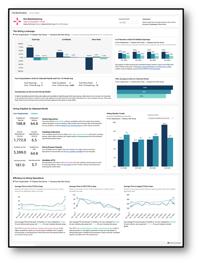
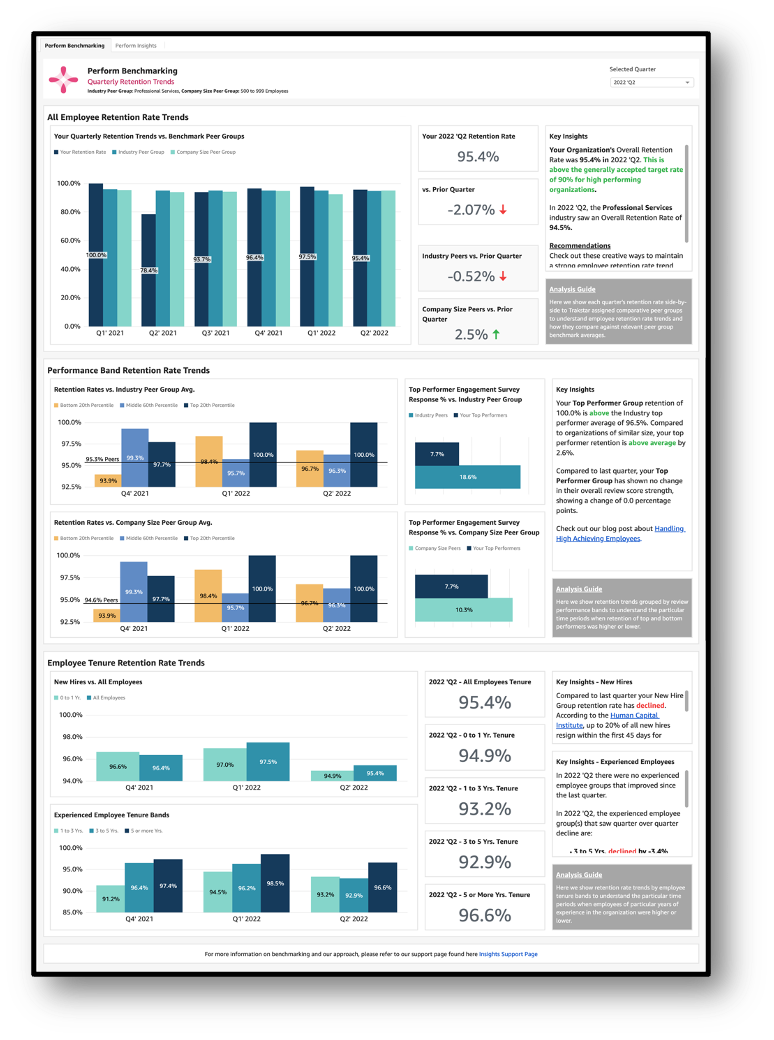
Brian Kasen is the Director, Business Intelligence at Mitratech. He is passionate about helping HR leaders be more data-driven in their efforts to hire, retain, and engage their employees. Prior to Mitratech, Brian spent much of his career building analytic solutions across a range of industries, including higher education, restaurant, and software.

Rebecca McAlpine is the Senior Product Manager for Trakstar Insights at Mitratech. Her experience in HR tech experience has allowed her to work in various areas, including data analytics, business systems optimization, candidate experience, job application management, talent engagement strategy, training, and performance management.

Large-scale digital biomarker computation with AWS serverless services

Post Syndicated from Avni Patel original https://aws.amazon.com/blogs/architecture/large-scale-digital-biomarker-computation-with-aws-serverless-services/

Digital biomarkers are quantitative, objective measures of physiological and behavioral data. They are collected and measured using digital devices that better represent free-living activity in contrast to a highly structured in-clinic setting. This approach generates large amounts of data that requires processing.

Digital biomarker data is typically saved in different formats, and various sources require different (and often multiple) processing steps. In 2020, the Digital Sciences and Translational Imaging group at Pfizer developed a specialized pipeline using AWS services for analyzing incoming sensor data from wrist devices for sleep and scratch activity.

In time, the original pipeline needed updating to compute digital biomarkers at scale while maintaining reproducibility and data provenance. The key component in re-designing the pipeline is flexibility so the platform can:

  • Handle various incoming data sources and different algorithms
  • Handle distinct sets of algorithm parameters

These goals were accomplished with a framework for handling file analysis that uses a two-part approach:

  1. A Python package using a custom common architecture
  2. An AWS-based pipeline to handle processing mapping and computing distribution

This blog post introduces this custom Python package data processing pipeline using AWS services. The AWS architecture maintains data provenance while enabling fast, efficient, and scalable data processing. These large data sets would otherwise consume significant local resources.

Let’s explore each part of this framework in detail.

Custom Python package for data processing

Computation of digital biomarkers requires specific algorithms. Typically, these algorithms—for example, gait, activity, and more—had separate code repositories. Little thought was given to interaction and reproducibility.

Pfizer addressed this issue by creating the SciKit-Digital-Health Python package (SKDH) to implement these algorithms and data ingestion methods. As the SKDH framework is designed with reproducibility and integration in mind, modules can be chained together in a pipeline structure and run sequentially. Pipelines can be saved and loaded later; a key feature in enabling dynamic pipeline selection and reproducibility.

AWS framework for file analysis

While SKDH is the core that computes the digital biomarkers, it requires an operational framework for handling all the data files. To that end, Pfizer and AWS designed the following architecture to handle file analysis on a study-by-study basis, as shown in Figure 1:

Digital biomarker catalog and file processing workflow

Figure 1. Digital biomarker catalog and file processing workflow

The overall platform can be broken into two components: the Catalog and File Processing AWS Step Functions workflows. Let’s explore each of these components, along with the necessary configuration file to process a study.

Catalog Step Functions workflow

The Catalog workflow searches study Amazon Simple Storage Service (Amazon S3) buckets for files that need processing. These files are defined in a study configuration document. The workflow consists of the following steps:

  1. The Catalog Step Function is manually triggered.
  2. If the study configuration file is found and the S3 Study buckets specified in the configuration file exist, search the S3 Study buckets for any files matching those enumerated in the study configuration file.
  3. If the configuration file or S3 Study bucket are not found, send a message to an Amazon Simple Queue Service (Amazon SQS) queue.
  4. For any cataloged files, start a new Processing workflow for each of these files.

File processing Step Functions workflow

The Processing workflow verifies processing requirements and processes both study data files and metadata files through the following steps:

  1. From the study configuration file, the workflow gets relevant details for the file. This includes metadata processing requirements as needed, and the specified set of SKDH algorithms to run.
  2. If the file contains metadata, a special AWS Lambda function cleans the data and saves it to the metadata Amazon DynamoDB table. Otherwise, check whether all requirements are met, including processing requirements (for example, height for gait algorithms) and logistics requirements (for example, file name information extraction functions).
  3. For missing requirements, the workflow will send a message to an Amazon SQS queue and try waiting for them to be met.
  4. If all requirements are met, it will start a batch job for the file.
  5. The batch job runs on AWS Fargate with a custom Docker image with a specified version of SKDH. This allows for easy versioning and reproducibility.
  6. The Docker image loads the specified SKDH pipeline and computes the digital biomarkers. Any results generated are then uploaded back to the S3 Study bucket at the end of processing.

Study configuration file

The configuration file defines everything necessary for processing a study. This includes which S3 bucket(s) the study data is located in, under which prefixes, and the list of file patterns of files to be processed. Figure 2 offers a sample configuration file example:

Sample study configuration file

Figure 2. Sample study configuration file

Building a stack with AWS CloudFormation

AWS CloudFormation provisions and configures all of the resources for the pipeline, allowing AWS services to be easily added and removed. CloudFormation integration with Github makes it easy to keep track of service changes. AWS Step Functions can also be integrated into CloudFormation template files, which gives an AWS specification in essentially one master file.

To iterate and update the stack, a combination of Python, Amazon SDK for Python (Boto3), and AWS Command Line Interface (AWS CLI) tools are used. Python allows for a more intricate command line script with positional and keyword arguments depending on the process. For example, updating the pipeline is a simple command, where <env> is the dev/stage/prod environment that needs to be updated:

Updating the pipeline with a simple command

Figure 3. Updating the pipeline with a simple command

Meanwhile, the Python function would be something like the following:

Sample Python function

Figure 4. Sample Python function

While it might seem unconventional to use both SDK for Python and a call to the AWS CLI from Python in the same script, the AWS CLI has some useful features that make the CloudFormation packaging and stack creation much easier. The end of the example file in Figure 3 pertains to the main utility in using the Python argparse package, which provides an easy to write user-friendly CLI.

This could also be achieved using AWS Cloud Development Kit (AWS CDK), an open source software development framework that allows you to define infrastucture in familiar programming languages. AWS CDK uses constructs that can be customized and reused.

Conclusion

This blog post shared a custom data processing pipeline using AWS services that, through intentional integration with a Python package, can run arbitrary algorithms to process data. By using AWS as the framework for this pipeline, data provenance is maintained while enabling fast, efficient, and scalable processing of large amounts of data that would typically consume significant company resources.

Automate alerting and reporting for AWS Glue job resource usage

Post Syndicated from Michael Hamilton original https://aws.amazon.com/blogs/big-data/automate-alerting-and-reporting-for-aws-glue-job-resource-usage/

Data transformation plays a pivotal role in providing the necessary data insights for businesses in any organization, small and large. To gain these insights, customers often perform ETL (extract, transform, and load) jobs from their source systems and output an enriched dataset. Many organizations today are using AWS Glue to build ETL pipelines that bring data from disparate sources and store the data in repositories like a data lake, database, or data warehouse for further consumption. These organizations are looking for ways they can reduce cost across their IT environments and still be operationally performant and efficient.

Picture a scenario where you, the VP of Data and Analytics, are in charge of your data and analytics environments and workloads running on AWS where you manage a team of data engineers and analysts. This team is allowed to create AWS Glue for Spark jobs in development, test, and production environments. During testing, one of the jobs wasn’t configured to automatically scale its compute resources, resulting in jobs timing out, costing the organization more than anticipated. The next steps usually include completing an analysis of the jobs, looking at cost reports to see which account generated the spike in usage, going through logs to see when what happened with the job, and so on. After the ETL job has been corrected, you may want to implement monitoring and set standard alert thresholds for your AWS Glue environment.

This post will help organizations proactively monitor and cost optimize their AWS Glue environments by providing an easier path for teams to measure efficiency of their ETL jobs and align configuration details according to organizational requirements. Included is a solution you will be able to deploy that will notify your team via email about any Glue job that has been configured incorrectly. Additionally, a weekly report is generated and sent via email that aggregates resource usage and provides cost estimates per job.

AWS Glue cost considerations

AWS Glue for Apache Spark jobs are provisioned with a number of workers and a worker type. These jobs can be either G.1X, G.2X, G.4X, G.8X or Z.2X (Ray) worker types that map to data processing units (DPUs). DPUs include a certain amount of CPU, memory, and disk space. The following table contains more details.

Worker Type DPUs vCPUs Memory (GB) Disk (GB)
G.1X 1 4 16 64
G.2X 2 8 32 128
G.4X 4 16 64 256
G.8X 8 32 128 512
Z.2X 2 8 32 128

For example, if a job is provisioned with 10 workers as G.1X worker type, the job will have access to 40 vCPU and 160 GB of RAM to process data and double using G.2X. Over-provisioning workers can lead to increased cost, due to not all workers being utilized efficiently.

In April 2022, Auto Scaling for AWS Glue was released for AWS Glue version 3.0 and later, which includes AWS Glue for Apache Spark and streaming jobs. Enabling auto scaling on your Glue for Apache Spark jobs will allow you to only allocate workers as needed, up to the worker maximum you specify. We recommend enabling auto scaling for your AWS Glue 3.0 & 4.0 jobs because this feature will help reduce cost and optimize your ETL jobs.

Amazon CloudWatch metrics are also a great way to monitor your AWS Glue environment by creating alarms for certain metrics like average CPU or memory usage. To learn more about how to use CloudWatch metrics with AWS Glue, refer to Monitoring AWS Glue using Amazon CloudWatch metrics.

The following solution provides a simple way to set AWS Glue worker and job duration thresholds, configure monitoring, and receive emails for notifications on how your AWS Glue environment is performing. If a Glue job finishes and detects worker or job duration thresholds were exceeded, it will notify you after the job run has completed, failed, or timed out.

Solution overview

The following diagram illustrates the solution architecture.

Solution Architecture

When you deploy this application via AWS Serverless Application Model (AWS SAM), it will ask what AWS Glue worker and job duration thresholds you would like to set to monitor the AWS Glue for Apache Spark and AWS Glue for Ray jobs running in that account. The solution will use these values as the decision criteria when invoked. The following is a breakdown of each step in the architecture:

  1. Any AWS Glue for Apache Spark job that succeeds, fails, stops, or times out is sent to Amazon EventBridge.
  2. EventBridge picks up the event from AWS Glue and triggers an AWS Lambda function.
  3. The Lambda function processes the event and determines if the data and analytics team should be notified about the particular job run. The function performs the following tasks:
    1. The function sends an email using Amazon Simple Notification Service (Amazon SNS) if needed.
      • If the AWS Glue job succeeded or was stopped without going over the worker or job duration thresholds, or is tagged to not be monitored, no alerts or notifications are sent.
      • If the job succeeded but ran with a worker or job duration thresholds higher than allowed, or the job either failed or timed out, Amazon SNS sends a notification to the designated email with information about the AWS Glue job, run ID, and reason for alerting, along with a link to the specific run ID on the AWS Glue console.
    2. The function logs the job run information to Amazon DynamoDB for a weekly aggregated report delivered to email. The Dynamo table has Time to Live enabled for 7 days, which keeps the storage to minimum.
  4. Once a week, the data within DynamoDB is aggregated by a separate Lambda function with meaningful information like longest-running jobs, number of retries, failures, timeouts, cost analysis, and more.
  5. Amazon Simple Email Service (Amazon SES) is used to deliver the report because it can be better formatted than using Amazon SNS. The email is formatted via HTML output that provides tables for the aggregated job run data.
  6. The data and analytics team is notified about the ongoing job runs through Amazon SNS, and they receive the weekly aggregation report through Amazon SES.

Note that AWS Glue Python shell and streaming ETL jobs are not supported because they’re not in scope of this solution.

Prerequisites

You must have the following prerequisites:

  • An AWS account to deploy the solution to
  • Proper AWS Identity and Access Management (IAM) privileges to create the resources
  • The AWS SAM CLI to build and deploy the solution button below, to run template on your AWS environment

Deploy the solution

This AWS SAM application provisions the following resources:

  • Two EventBridge rules
  • Two Lambda functions
  • An SNS topic and subscription
  • A DynamoDB table
  • An SES subscription
  • The required IAM roles and policies

To deploy the AWS SAM application, complete the following steps:

Clone the aws-samples GitHub repository:

git clone https://github.com/aws-samples/aws-glue-job-tracker.git

Deploy the AWS SAM application:

cd aws-glue-job-tracker
sam deploy --guided

sam deploy configuration

Provide the following parameters:

  • GlueJobWorkerThreshold – Enter the maximum number of workers you want an AWS Glue job to be able to run with before sending threshold alert. The default is 10. An alert will be sent if a Glue job runs with higher workers than specified.
  • GlueJobDurationThreshold – Enter the maximum duration in minutes you want an AWS Glue job to run before sending threshold alert. The default is 480 minutes (8 hours). An alert will be sent if a Glue job runs with higher job duration than specified.
  • GlueJobNotifications – Enter an email or distribution list of those who need to be notified through Amazon SNS and Amazon SES. You can go to the SNS topic after the deployment is complete and add emails as needed.

To receive emails from Amazon SNS and Amazon SES, you must confirm your subscriptions. After the stack is deployed, check your email that was specified in the template and confirm by choosing the link in each message. When the application is successfully provisioned, it will begin monitoring your AWS Glue for Apache Spark job environment. The next time a job fails, times out, or exceeds a specified threshold, you will receive an email via Amazon SNS. For example, the following screenshot shows an SNS message about a job that succeeded but had a job duration threshold violation.

You might have jobs that need to run at a higher worker or job duration threshold, and you don’t want the solution to evaluate them. You can simply tag that job with the key/value of remediate and false. The step function will still be invoked, but will use the PASS state when it recognizes the tag. For more information on job tagging, refer to AWS tags in AWS Glue.

Adding tags to glue job configuration

Configure weekly reporting

As mentioned previously, when an AWS Glue for Apache Spark job succeeds, fails, times out, or is stopped, EventBridge forwards this event to Lambda, where it logs specific information about each job run. Once a week, a separate Lambda function queries DynamoDB and aggregates your job runs to provide meaningful insights and recommendations about your AWS Glue for Apache Spark environment. This report is sent via email with a tabular structure as shown in the following screenshot. It’s meant for top-level visibility so you’re able to see your longest job runs over time, jobs that have had many retries, failures, and more. It also provides an overall cost calculation as an estimate of what each AWS Glue job will cost for that week. It should not be used as a guaranteed cost. If you would like to see exact cost per job, the AWS Cost and Usage Report is the best resource to use. The following screenshot shows one table (of five total) from the AWS Glue report function.

weekly report

Clean up

If you don’t want to run the solution anymore, delete the AWS SAM application for each account that it was provisioned in. To delete your AWS SAM stack, run the following command from your project directory:

sam delete

Conclusion

In this post, we discussed how you can monitor and cost-optimize your AWS Glue job configurations to comply with organizational standards and policy. This method can provide cost controls over AWS Glue jobs across your organization. Some other ways to help control the costs of your AWS Glue for Apache Spark jobs include the newly released AWS Glue Flex jobs and Auto Scaling. We also provided an AWS SAM application as a solution to deploy into your accounts. We encourage you to review the resources provided in this post to continue learning about AWS Glue. To learn more about monitoring and optimizing for cost using AWS Glue, please visit this recent blog. It goes in depth on all of the cost optimization options and includes a template that builds a CloudWatch dashboard for you with metrics about all of your Glue job runs.


About the authors

Michael Hamilton is a Sr Analytics Solutions Architect focusing on helping enterprise customers in the south east modernize and simplify their analytics workloads on AWS. He enjoys mountain biking and spending time with his wife and three children when not working.

Angus Ferguson is a Solutions Architect at AWS who is passionate about meeting customers across the world, helping them solve their technical challenges. Angus specializes in Data & Analytics with a focus on customers in the financial services industry.

Defontana provides business administration solutions to Latin American customers using Amazon QuickSight

Post Syndicated from Cynthia Valeriano original https://aws.amazon.com/blogs/big-data/defontana-provides-business-administration-solutions-to-latin-american-customers-using-amazon-quicksight/

This is a guest post by Cynthia Valeriano, Jaime Olivares, and Guillermo Puelles from DeFontana.

Defontana develops fully cloud-based business applications for the administration and management of companies. Based in Santiago, Chile, with operations in Peru, Mexico, and most recently Colombia, our main product is a 100% cloud-based enterprise resource planning (ERP) system that has been providing value to our business customers for about 20 years. In addition to our core ERP product, we have developed integration modules for ecommerce, banks, financial and regulatory institutions, digital signatures, business reports, and many other solutions. Our goal is to continue building solutions for customers and make Defontana the best business administration tool in Chile and Latin America.

Most of our customers are small and medium businesses (SMBs) who need to optimize their resources. Our ERP system helps customers manage cash flow, time, human resources (HR), and other resources. As we were exploring how to continue innovating for our customers and looking for an embedded analytics solution, we chose Amazon QuickSight, which allows us to seamlessly integrate data-driven experiences into our web application.

In this post, we discuss how QuickSight has sped up our development time, enabled us to provide more value to our customers, and even improved our own internal operations.

Saving development time by embedding QuickSight

We built our ERP service as a web application from the beginning. 10 years ago, this was a big differentiator for us, but to continue to serve the SMBs that trust us for information on a daily basis, we wanted to offer even more advanced analytics. By embedding QuickSight into our web application, we have been able to provide business intelligence (BI) functionalities to customers two or three times faster than we would have if we had opted for libraries for generating HTML reports. Thanks to our embedded QuickSight solution, we are able to focus more of our energy on analyzing the requirements and functionalities that we want to offer our customers in each BI report.

The following screenshots show our ERP service, accessed on a web browser, with insights and rich visualizations by QuickSight.

We enjoy using QuickSight because of how well it integrates with other AWS services. Our data is stored in a legacy relational database management system (RDMS), Amazon Aurora, and Amazon DynamoDB. We are in the process of moving away from that legacy RDMS to PostgreSQL through a Babelfish for Aurora PostgreSQL project. This will allow us to reduce costs while also being able to use a multi-Region database with disaster recovery in the future. This would have been too expensive with the legacy RDMS. To seamlessly transfer data from these databases to Amazon Simple Storage Service (Amazon S3), we use AWS Database Migration Service (AWS DMS). Then, AWS Glue allows us to generate several extract, transform, and load (ETL) processes to prepare the data in Amazon S3 to be used in QuickSight. Finally, we use Amazon Athena to generate views to be used as base information in QuickSight.

Providing essential insights for SMB customers

QuickSight simplifies the generation of dashboards. We have made several out-of-the-box dashboards in QuickSight for our customers that they can use directly on our web app right after they sign up. These dashboards provide insights on sales, accounting, cash flow, financial information, and customer clusters based on their data in our ERP service. These free-to-use reports can be used by all customers in the system. We also have dashboards that can be activated by any user of the system for a trial period. Since we launched add-on dashboards, more than 300 companies have activated it, with over 100 of them choosing to continue using it after the free trial.

Besides generic reports, we have created several tailor-made dashboards according to the specific requirements of each customer. These are managed through a customer-focused development process by our engineering team according to the specifications of each customer. With this option, our customers can get reports on accounts payable, accounts receivable, supply information (purchase order flow, receipts and invoices sent by suppliers), inventory details, and more. We have more than 50 customers who have worked with us on tailor-made dashboards. With the broad range of functionalities within QuickSight, we can offer many data visualization options to our customers.

Empowering our own operations

Beyond using QuickSight to serve our customers, we also use QuickSight for our own BI reporting. So far, we have generated more than 80 dashboards to analyze different business flows. For example, we monitor daily sales in specific services, accounting, software as a service (SaaS) metrics, and the operation of our customers. We do all of this from within our own web application, with the power of QuickSight, giving us the opportunity to experience the interface just like our customers do. In 2023, one of our top goals is to provide a 360-degree view of Defontana using QuickSight.

Conclusion

QuickSight has enabled us to seamlessly embed analytics into our ERP service, providing valuable insights to our SMB customers. We have been able to cut costs and continue to grow throughout Latin America. We plan to use QuickSight even more within our own organization, making us more data-driven. QuickSight will empower us to democratize the information that our own employees receive, establish better processes, and create more tools to analyze customer information for behavioral patterns, which we can use to better meet our customers’ needs.

To learn more about how you can embed customized data visuals and interactive dashboards into any application, visit Amazon QuickSight Embedded.


About the authors

Cynthia Valeriano is a Business Intelligence Developer of at Defontana, with skills focused on data analysis and visualization. With 3 years of experience in administrative areas and 2 years of experience in business intelligence projects, she has been in charge of implementing data migration and transformation tasks with various AWS tools, such as AWS DMS and AWS Glue, in addition to generating multiple dashboards in Amazon QuickSight.

Jaime Olivares is a Senior software developer at Defontana, with 6 years of experience in the development of various technologies focused on the analysis of solutions and customer requirements. Experience with AWS in various services, including product development through QuickSight for the analysis of business and accounting data.

Guillermo Puelles is a Technical Manager of the “Appia” Integrations team at Defontana, with 9 years of experience in software development and 5 years working with AWS tools. Responsible for planning and managing various projects for the implementation of BI solutions through QuickSight and other AWS services.

Reserving EC2 Capacity across Availability Zones by utilizing On Demand Capacity Reservations (ODCRs)

Post Syndicated from Sheila Busser original https://aws.amazon.com/blogs/compute/reserving-ec2-capacity-across-availability-zones-by-utilizing-on-demand-capacity-reservations-odcrs/

This post is written by Johan Hedlund, Senior Solutions Architect, Enterprise PUMA.

Many customers have successfully migrated business critical legacy workloads to AWS, utilizing services such as Amazon Elastic Compute Cloud (Amazon EC2), Auto Scaling Groups (ASGs), as well as the use of Multiple Availability Zones (AZs), Regions for Business Continuity, and High Availability.

These critical applications require increased levels of availability to meet strict business Service Level Agreements (SLAs), even in extreme scenarios such as when EC2 functionality is impaired (see Advanced Multi-AZ Resilience Patterns for examples). Following AWS best practices such as architecting for flexibility will help here, but for some more rigid designs there can still be challenges around EC2 instance availability.

In this post, I detail an approach for Reserving Capacity for this type of scenario to mitigate the risk of the instance type(s) that your application needs being unavailable, including code for building it and ways of testing it.

Baseline: Multi-AZ application with restrictive instance needs

To focus on the problem of Capacity Reservation, our reference architecture is a simple horizontally scalable monolith. This consists of a single executable running across multiple instances as a cluster in an Auto Scaling group across three AZs for High Availability.

Architecture diagram featuring an Auto Scaling Group spanning three Availability Zones within one Region for high availability.

The application in this example is both business critical and memory intensive. It needs six r6i.4xlarge instances to meet the required specifications. R6i has been chosen to meet the required memory to vCPU requirements.

The third-party application we need to run, has a significant license cost, so we want to optimize our workload to make sure we run only the minimally required number of instances for the shortest amount of time.

The application should be resilient to issues in a single AZ. In the case of multi-AZ impact, it should failover to Disaster Recovery (DR) in an alternate Region, where service level objectives are instituted to return operations to defined parameters. But this is outside the scope for this post.

The problem: capacity during AZ failover

In this solution, the Auto Scaling Group automatically balances its instances across the selected AZs, providing a layer of resilience in the event of a disruption in a single AZ. However, this hinges on those instances being available for use in the Amazon EC2 capacity pools. The criticality of our application comes with SLAs which dictate that even the very low likelihood of instance types being unavailable in AWS must be mitigated.

The solution: Reserving Capacity

There are 2 main ways of Reserving Capacity for this scenario: (a) Running extra capacity 24/7, (b) On Demand Capacity Reservations (ODCRs).

In the past, another recommendation would have been to utilize Zonal Reserved Instances (Non Zonal will not Reserve Capacity). But although Zonal Reserved Instances do provide similar functionality as On Demand Capacity Reservations combined with Savings Plans, they do so in a less flexible way. Therefore, the recommendation from AWS is now to instead use On Demand Capacity Reservations in combination with Savings Plans for scenarios where Capacity Reservation is required.

The TCO impact of the licensing situation rules out the first of the two valid options. Merely keeping the spare capacity up and running all the time also doesn’t cover the scenario in which an instance needs to be stopped and started, for example for maintenance or patching. Without Capacity Reservation, there is a theoretical possibility that that instance type would not be available to start up again.

This leads us to the second option: On Demand Capacity Reservations.

How much capacity to reserve?

Our failure scenario is when functionality in one AZ is impaired and the Auto Scaling Group must shift its instances to the remaining AZs while maintaining the total number of instances. With a minimum requirement of six instances, this means that we need 6/2 = 3 instances worth of Reserved Capacity in each AZ (as we can’t know in advance which one will be affected).

Illustration of number of instances required per Availability Zone, in order to keep the total number of instances at six when one Availability Zone is removed. When using three AZs there are two instances per AZ. When using two AZs there are three instances per AZ.

Spinning up the solution

If you want to get hands-on experience with On Demand Capacity Reservations, refer to this CloudFormation template and its accompanying README file for details on how to spin up the solution that we’re using. The README also contains more information about the Stack architecture. Upon successful creation, you have the following architecture running in your account.

Architecture diagram featuring adding a Resource Group of On Demand Capacity Reservations with 3 On Demand Capacity Reservations per Availability Zone.

Note that the default instance type for the AWS CloudFormation stack has been downgraded to t2.micro to keep our experiment within the AWS Free Tier.

Testing the solution

Now we have a fully functioning solution with Reserved Capacity dedicated to this specific Auto Scaling Group. However, we haven’t tested it yet.

The tests utilize the AWS Command Line Interface (AWS CLI), which we execute using AWS CloudShell.

To interact with the resources created by CloudFormation, we need some names and IDs that have been collected in the “Outputs” section of the stack. These can be accessed from the console in a tab under the Stack that you have created.

Example of outputs from running the CloudFormation stack. AutoScalingGroupName, SubnetForManuallyAddedInstance, and SubnetsToKeepWhenDroppingASGAZ.

We set these as variables for easy access later (replace the values with the values from your stack):

export AUTOSCALING_GROUP_NAME=ASGWithODCRs-CapacityBackedASG-13IZJWXF9QV8E
export SUBNET_FOR_MANUALLY_ADDED_INSTANCE=subnet-03045a72a6328ef72
export SUBNETS_TO_KEEP=subnet-03045a72a6328ef72,subnet-0fd00353b8a42f251

How does the solution react to scaling out the Auto Scaling Group beyond the Capacity Reservation?

First, let’s look at what happens if the Auto Scaling Group wants to Scale Out. Our requirements state that we should have a minimum of six instances running at any one time. But the solution should still adapt to increased load. Before knowing anything about how this works in AWS, imagine two scenarios:

  1. The Auto Scaling Group can scale out to a total of nine instances, as that’s how many On Demand Capacity Reservations we have. But it can’t go beyond that even if there is On Demand capacity available.
  2. The Auto Scaling Group can scale just as much as it could when On Demand Capacity Reservations weren’t used, and it continues to launch unreserved instances when the On Demand Capacity Reservations run out (assuming that capacity is in fact available, which is why we have the On Demand Capacity Reservations in the first place).

The instances section of the Amazon EC2 Management Console can be used to show our existing Capacity Reservations, as created by the CloudFormation stack.

Listing of consumed Capacity Reservations across the three Availability Zones, showing two used per Availability Zone.

As expected, this shows that we are currently using six out of our nine On Demand Capacity Reservations, with two in each AZ.

Now let’s scale out our Auto Scaling Group to 12, thus using up all On Demand Capacity Reservations in each AZ, as well as requesting one extra Instance per AZ.

aws autoscaling set-desired-capacity \
--auto-scaling-group-name $AUTOSCALING_GROUP_NAME \
--desired-capacity 12

The Auto Scaling Group now has the desired Capacity of 12:

Group details of the Auto Scaling Group, showing that Desired Capacity is set to 12.

And in the Capacity Reservation screen we can see that all our On Demand Capacity Reservations have been used up:

Listing of consumed Capacity Reservations across the three Availability Zones, showing that all nine On Demand Capacity Reservations are used.

In the Auto Scaling Group we see that – as expected – we weren’t restricted to nine instances. Instead, the Auto Scaling Group fell back on launching unreserved instances when our On Demand Capacity Reservations ran out:

Listing of Instances in the Auto Scaling Group, showing that the total count is 12.

How does the solution react to adding a matching instance outside the Auto Scaling Group?

But what if someone else/another process in the account starts an EC2 instance of the same type for which we have the On Demand Capacity Reservations? Won’t they get that Reservation, and our Auto Scaling Group will be left short of its three instances per AZ, which would mean that we won’t have enough reservations for our minimum of six instances in case there are issues with an AZ?

This all comes down to the type of On Demand Capacity Reservation that we have created, or the “Eligibility”. Looking at our Capacity Reservations, we can see that they are all of the “targeted” type. This means that they are only used if explicitly referenced, like we’re doing in our Target Group for the Auto Scaling Group.

Listing of existing Capacity Reservations, showing that they are of the targeted type.

It’s time to prove that. First, we scale in our Auto Scaling Group so that only six instances are used, resulting in there being one unused capacity reservation in each AZ. Then, we try to add an EC2 instance manually, outside the target group.

First, scale in the Auto Scaling Group:

aws autoscaling set-desired-capacity \
--auto-scaling-group-name $AUTOSCALING_GROUP_NAME \
--desired-capacity 6

Listing of consumed Capacity Reservations across the three Availability Zones, showing two used reservations per Availability Zone.

Listing of Instances in the Auto Scaling Group, showing that the total count is six

Then, spin up the new instance, and save its ID for later when we clean up:

export MANUALLY_CREATED_INSTANCE_ID=$(aws ec2 run-instances \
--image-id resolve:ssm:/aws/service/ami-amazon-linux-latest/amzn2-ami-hvm-x86_64-gp2 \
--instance-type t2.micro \
--subnet-id $SUBNET_FOR_MANUALLY_ADDED_INSTANCE \
--query 'Instances[0].InstanceId' --output text) 

Listing of the newly created instance, showing that it is running.

We still have the three unutilized On Demand Capacity Reservations, as expected, proving that the On Demand Capacity Reservations with the “targeted” eligibility only get used when explicitly referenced:

Listing of consumed Capacity Reservations across the three Availability Zones, showing two used reservations per Availability Zone.

How does the solution react to an AZ being removed?

Now we’re comfortable that the Auto Scaling Group can grow beyond the On Demand Capacity Reservations if needed, as long as there is capacity, and that other EC2 instances in our account won’t use the On Demand Capacity Reservations specifically purchased for the Auto Scaling Group. It’s time for the big test. How does it all behave when an AZ becomes unavailable?

For our purposes, we can simulate this scenario by changing the Auto Scaling Group to be across two AZs instead of the original three.

First, we scale out to seven instances so that we can see the impact of overflow outside the On Demand Capacity Reservations when we subsequently remove one AZ:

aws autoscaling set-desired-capacity \
--auto-scaling-group-name $AUTOSCALING_GROUP_NAME \
--desired-capacity 7

Then, we change the Auto Scaling Group to only cover two AZs:

aws autoscaling update-auto-scaling-group \
--auto-scaling-group-name $AUTOSCALING_GROUP_NAME \
--vpc-zone-identifier $SUBNETS_TO_KEEP

Give it some time, and we see that the Auto Scaling Group is now spread across two AZs, On Demand Capacity Reservations cover the minimum six instances as per our requirements, and the rest is handled by instances without Capacity Reservation:

Network details for the Auto Scaling Group, showing that it is configured for two Availability Zones.

Listing of consumed Capacity Reservations across the three Availability Zones, showing two Availability Zones using three On Demand Capacity Reservations each, with the third Availability Zone not using any of its On Demand Capacity Reservations.

Listing of Instances in the Auto Scaling Group, showing that there are 4 instances in the eu-west-2a Availability Zone.

Cleanup

It’s time to clean up, as those Instances and On Demand Capacity Reservations come at a cost!

  1. First, remove the EC2 instance that we made:
    aws ec2 terminate-instances --instance-ids $MANUALLY_CREATED_INSTANCE_ID
  2. Then, delete the CloudFormation stack.

Conclusion

Using a combination of Auto Scaling Groups, Resource Groups, and On Demand Capacity Reservations (ODCRs), we have built a solution that provides High Availability backed by reserved capacity, for those types of workloads where the requirements for availability in the case of an AZ becoming temporarily unavailable outweigh the increased cost of reserving capacity, and where the best practices for architecting for flexibility cannot be followed due to limitations on applicable architectures.

We have tested the solution and confirmed that the Auto Scaling Group falls back on using unreserved capacity when the On Demand Capacity Reservations are exhausted. Moreover, we confirmed that targeted On Demand Capacity Reservations won’t risk getting accidentally used by other solutions in our account.

Now it’s time for you to try it yourself! Download the IaC template and give it a try! And if you are planning on using On Demand Capacity Reservations, then don’t forget to look into Savings Plans, as they significantly reduce the cost of that Reserved Capacity..

Softbrain provides advanced analytics to sales customers with Amazon QuickSight

Post Syndicated from Kenta Oda original https://aws.amazon.com/blogs/big-data/softbrain-provides-advanced-analytics-to-sales-customers-with-amazon-quicksight/

This is a guest post by Kenta Oda from SOFTBRAIN Co., Ltd.

Softbrain is a leading Japanese producer of software for sales force automation (SFA) and customer relationship management (CRM). Our main product, e-Sales Manager (eSM), is an SFA/CRM tool that provides sales support to over 5,500 companies in Japan. We provide our sales customers with a one-stop source for information and visualization of sales activity, improving their efficiency and agility, which leads to greater business opportunity.

With increasing demand from our customers for analyzing data from different angles throughout the sales process, we needed an embedded analytics tool. We chose Amazon QuickSight, a cloud-native business intelligence (BI) tool that allows you to embed insightful analytics into any application with customized, interactive visuals and dashboards. It integrates seamlessly with eSM and is easy to use at a low cost.

In this post, we discuss how QuickSight is helping us provide our sales customers with the insights they need, and why we consider this business decision a win for Softbrain.

There were four things we were looking for in an embedded analytics solution:

  • Rich visualization – With our previous solution, which was built in-house, there were only four types of visuals, so it was difficult to combine multiple graphs for an in-depth analysis.
  • Development speed – We needed to be able to quickly implement BI functionalities. QuickSight requires minimal development due to its serverless architecture, embedding, and API.
  • Cost – We moved from Tableau to QuickSight because QuickSight allowed us to provide data analysis and visualizations to our customers at a competitive price—ensuring that more of our customers can afford it.
  • Ease of use – QuickSight is cloud-based and has an intuitive UX for our sales customers to work with.

Innovating with QuickSight

Individual productivity must be greatly improved to keep up with the shifting labor market in Japan. At Softbrain, we aim to innovate using the latest technology to provide science-based insights into customer and sales interactions, enabling those who use eSM to be much more productive. Sales reps and managers are able to make informed decisions.

By using QuickSight as our embedded analytics solution, we can offer data visualizations at a much lower price point, making it much more accessible for our customers than we could with other BI solutions. When we combine the process management system offered by eSM with the intuitive user experience and rich visualization capability of QuickSight, we empower customers to understand their sales data, which sits in Amazon Simple Storage Service (Amazon S3) and Amazon Aurora, and act on it.

Seamless console embedding

What sets QuickSight apart from other BI tools is console embedding, which means our customers have the ability to build their own dashboards within eSM. They can choose which visualizations they want and take an in-depth look at their data. Sales strategy requires agility, and our customers need more than a fixed dashboard. QuickSight offers freedom and flexibility with console embedding.

Console embedding allows eSM to be a one-stop source for all the information sales reps and managers need. They can access all the analyses they need to make decisions right from their web browser because QuickSight is fully managed and serverless. With other BI solutions, the user would need to have the client application installed on their computer to create their own dashboards.

Empowering our sales customers

With insights from QuickSight embedded into eSM, sales reps can analyze the gap between their budget and actual revenue to build an action plan to fill the gap. They can use their dashboards to analyze data on a weekly and monthly basis. They can share this information at meetings and explore the data to figure out why there might be low attainment for certain customers. Our customers can use eSM and QuickSight to understand why win or loss opportunities are increasing. Managers can analyze and compare the performance of their sales reps to learn what high-performing reps are doing and help low performers. Sales reps can also evaluate their own performance.

Driving 95% customer retention rate

All of these insights come from putting sales data into eSM and QuickSight. It’s no secret that our customers love QuickSight. We can boast a 95% customer retention rate and offer QuickSight as an embedded BI solution at largest scale in Japan.

To learn more about how you can embed customized data visuals and interactive dashboards into any application, visit Amazon QuickSight Embedded.


About the author

Kenta Oda is the Chief Technology Officer at SOFTBRAIN Co., Ltd. He is in responsible of new product development with keen insight on better customer experience and go-to-market strategy.

Peloton embraces Amazon Redshift to unlock the power of data during changing times

Post Syndicated from Phil Goldstein original https://aws.amazon.com/blogs/big-data/peloton-embraces-amazon-redshift-to-unlock-the-power-of-data-during-changing-times/

Jerry Wang, Peloton’s Director of Data Engineering (left), and Evy Kho, Peloton's Manager of Subscription Analytics, discuss how the company has benefited from using Amazon Redshift.

Credit: Phil Goldstein
Jerry Wang, Peloton’s Director of Data Engineering (left), and Evy Kho, Peloton’s Manager of Subscription Analytics, discuss how the company has benefited from using Amazon Redshift.

New York-based Peloton, which aims to help people around the world reach their fitness goals through its connected fitness equipment and subscription-based classes, saw booming growth in the early stage of the COVID-19 pandemic. In 2020, as gyms shuttered and people looked for ways to stay active from the safety of their homes, the company’s annual revenue soared from $915 million in 2019 to $4 billion in 2021. Meanwhile, the company’s subscribers jumped from around 360,000 in 2019 to 2.76 million at the end of 2022.

As Peloton’s business continued to evolve amid a changing macroeconomic environment, it was essential that it could make smart business decisions quickly, and one of the best ways to do that was to harness insights from the huge amount of data that it had been gathering over recent years.

During that same time, AWS has been focused on helping customers manage their ever-growing volumes of data with tools like Amazon Redshift, the first fully managed, petabyte-scale cloud data warehouse. The service has grown into a multifaceted service used by tens of thousands of customers to process exabytes of data on a daily basis (1 exabyte is equivalent to 119 billion song downloads). With Amazon Redshift, you get access to a modern data architecture that helps you break down internal data silos, share data securely and seamlessly, and support multiple users who don’t have specialized data and analytics skills.

When Jerry Wang, Peloton’s director of data engineering, joined the company in 2019, he needed to make sure the service would handle the company’s massive and growing amounts of data. He also needed to ensure Amazon Redshift could help the company efficiently manage the wide variety of data and the users who would need to access it, and deliver insights on that data at high velocity—all while being cost-effective and secure.

Wang was delighted to see that as Peloton experienced its massive growth and change, AWS continued to release new Amazon Redshift features and associated capabilities that would perfectly suit his company’s needs at just the right time.

“Over the years, I’ve always been in the stage where I hope Redshift can have a new, specific feature,” Wang says, “and then, in a very limited amount of time, AWS releases that kind of feature.”

Peloton’s data volumes soar as the business grows

Man working out with a weight while viewing a Peloton class on his TV in a living room.

Credit: Peloton

As Peloton’s business has evolved, the amount of data it is generating and analyzing has grown exponentially. From 2019 to now, Wang reports the amount of data the company holds has grown by a factor of 20. In fact, a full 95% of the total historical data the company has generated has come in the last 4 years. This growth has been driven both by surges in the number of users on Peloton’s platform and the variety of data the company is collecting.

Peloton collects reams of data on its sales of internet-connected exercise equipment like stationary bikes and treadmills. The company also collects data on customers’ workouts, which it then provides back to them in various reports such as a monthly summary, giving them insights into how often they worked out, their best output, trends in their workouts, the instructor they used the most, how many calories they burned, and more. All of this data helps Peloton make strategic business decisions, refine its operations to become more efficient, adjust its programming, and drive subscriber engagement and growth.

In 2019 and into 2020, as Peloton’s business boomed, the company needed an analytics system that could help it manage an explosion of data, both from users and related to its business. The company embraced Amazon Redshift because of the service’s versatility, ease of use, price-performance at scale, continuous pace of innovation, and ability to handle concurrent queries from dozens of internal data teams.

Wang said that when he joined the company, there were two kinds of users who were performing daily data operations in Peloton’s Amazon Redshift data warehouse. One group performed extract, transform, and load (ETL) operations to take raw data and make it available for analysis. The other was a group of business users who, each morning, would perform queries to generate local data visualizations, creating a surge of capacity on the Amazon Redshift data warehouse. “So, when these two loads ran together, the performance suffered directly,” Wang says.

One of the features Peloton adopted was Amazon Redshift Concurrency Scaling, which provides consistent and fast query performance even across thousands of concurrent users and concurrent queries. This helped solve the problem by automatically adding query processing power in seconds and processing queries without delays. When the workload demand subsided, the extra processing power was automatically removed, so Peloton only had to pay for the time when Concurrency Scaling data warehouses were in use. Wang says Peloton was running about 10 hours of Concurrency Scaling on a consistent daily basis to deal with the congestion, which, he says, “solved my problem at that moment.”

In 2020, as the pandemic inspired hoards to hop on bikes in their living rooms, Wang also upgraded Amazon Redshift with the newly introduced Amazon Redshift RA3 instances with managed storage (RMS). These represented a new generation of compute instances with managed, analytics-optimized storage designed for high-transaction, fast query performance and lower costs.

“The new instance … was a great feature for us,” Wang says. “It solved our concern about moving from terabyte scale to petabyte scale.”

Peloton’s business is driven by a variety of data for a wide range of users

Man watching a female Peloton biking instructor through a touch screen display on his Peloton bike.

Credit: Peloton

Peloton’s business model is driven by a wide variety of large volumes of data. In addition to selling bikes, treadmills, and indoor rowing machines, and expanding its subscription platform to include non-equipment-based workouts, the company has dozens of instructors in five countries, and it licenses music from three major music licensors. In 2022, it began renting bikes as well as selling them. Internally, Peloton employees working in finance, accounting, marketing, supply chain operations, music and content, and more are using data to track subscriber growth, content engagement, and which sales channels are leading to the most net new subscriptions.

“There was a time when we were just a bike company, and now we’re so much more than that,” says Evy Kho, manager of subscription analytics at Peloton.

There is also a much wider range of sales channels for Peloton equipment than just a few years ago. In the past, Peloton customers could only purchase bikes through the Peloton website or secondhand. Now, customers can purchase hardware from third-party sites like Amazon. That introduced “a really interesting data problem” for Peloton, says Kho, as it strives to determine how to link subscription signups back to exercise equipment sales.

In the face of this variability, complexity, and need for instant access to data to inform business decision-makers, Peloton embraced Amazon Redshift Serverless as an early adopter after AWS introduced the feature in late 2021. Redshift Serverless allows companies to quickly run and scale analytics capacity without database managers and data engineers needing to manage data warehouse infrastructure.

Redshift Serverless also has the ability to quickly spin up analytics capacity for different users, or personas, within an organization. This allows different teams across Peloton to perform analytics on the same datasets at the same time to generate insights on their individual parts of the business. It’s “incredibly important in terms of assessing what’s been good for our business,” Kho says.

Wang also says Peloton is considering supporting specific personas for those who need analytics around financial information governed by securities regulations, and another for users who need to perform analytics on data governed by regulations around personally identifiable information (PII).

Wang points out that Redshift Serverless also allows him to spin up Amazon Redshift data warehouses to handle special usage patterns. For example, ETL loads are often high I/O but require low CPU resources, and are very predictable because Peloton controls the process. However, when internal users want to perform data analytics or machine learning, the company doesn’t have control over the demand for those queries, and the load on Amazon Redshift data warehouses can be variable, with some queries more CPU-intensive than others. Previously, any provisioned data warehouse would have a fixed cost, and it would have to be provisioned to cope with the highest possible workloads even if the utilization rates turned out to be low. Now, for these different scenarios, Wang creates different Amazon Redshift instances to handle that variability without those heavy, fixed costs.

As Peloton’s use of Amazon Redshift has evolved and matured, its costs have gone down, according to Wang. “If you look at Serverless, the amount … that we spend on the Serverless is actually much smaller than we did previously, compared to the Concurrency Scaling cost.”

In a serverless environment, there is no upfront cost to Peloton. “I can set it up as quickly as I can and we pay as we need it,” Wang says. “It scales up when the load goes up. So, it’s a perfect fit.”

Peloton uses Amazon Redshift to get to insights faster

Women running on a Peloton treadmill with a touch screen display

Credit: Peloton

Peloton’s focus on efficiency and sustainable growth has meant that it needs to act more quickly than ever to make sound, data-informed business decisions. Peloton, Wang notes, is long past the stage where all it cared about was growth. “We are a mature company now, so operational efficiency is very important; it’s key to the business,” he says.

When Peloton launches new products, for example, two things typically happen, Wang says. One is that there is a spike in data volumes, both in traffic to its website and the number of sales transactions it’s processing. The second is that the company’s management team will want real-time updates and analysis of how sales are performing.

Redshift Serverless and data sharing lets users quickly start performing real-time analytics and build reporting and dashboard applications without any additional engineering required. Wang confirms this benefit, especially in the example of a new product launch, saying it “will scale up by itself without me having to intervene. I don’t need to allocate a budget. I don’t need to change any configurations.”

In the past, when Peloton only offered its fitness equipment through its own website, it was easy to associate fulfillment data on orders with subscriptions. However, as those channels grew and became more complex, Peloton turned to the data sharing capabilities of Amazon Redshift to share data quickly and easily across teams. Peloton’s teams for subscriber analytics, supply chain, accounting, and more need fast access to fulfillment data to ensure they can track it accurately, respond if changes are needed, and determine how fulfillment data aligns with subscriptions and revenue.

“Getting them those results even faster has been incredibly helpful, and is only becoming more important as we have become far more data-driven than I think you could argue we were before,” Kho says.

Amazon Redshift marries data security, governance, and compliance with innovation

Like all customers, Peloton is concerned about data security, governance, and compliance. With security features like dynamic data masking, role-based access control, and row-level security, Amazon Redshift protects customers’ data with granular authorization features and comprehensive identity management.

Customers also are able to easily provide authorizations for the right users or groups. These features are available out of the box, within the standard pricing model.

Wang notes that Amazon Redshift’s security model is based on a traditional database model, which is a well-understood and robust model. “So for us, to provision access on that model is quite straightforward,” Wang says.

At every stage of Peloton’s evolution over the last 4 years, the company has been able to turn to AWS and Amazon Redshift to help it effectively manage that growth and complexity.

“When I started,” Wang says, “I said, OK, I need a temporary boost in capacity. Then came Concurrency Scaling. And then I said, I need cheaper storage, and [RA3] comes along. And then the ultimate challenge [was], I’m no longer satisfied with a monolithic Redshift instance. Serverless solved that issue.”

Join AWS Data Insights Day 2023

If you want to learn how your company can use Amazon Redshift to analyze large volumes of data in an easy-to-use, scalable, cost-effective, and secure way, don’t miss AWS Data Insights Day on May 24, 2023. During the day-long virtual event, learn from AWS leaders, experts, partners, and customers—including Peloton, Gilead, McDonald’s, Global Foundries, Schneider Electric, and Flutter Entertainment—how Amazon Redshift and features like Amazon Redshift ML are helping drive business innovation, optimization, and cost savings, especially in today’s uncertain economic times.

Register Now for a calendar reminder.

To learn more about Amazon Redshift, see Amazon Redshift and Amazon Redshift: Ten years of continuous reinvention.


About the author

Phil Goldstein is a copywriter and editor with AWS product marketing. He has 15 years of technology writing experience, and prior to joining AWS was a senior editor at a content marketing agency and a business journalist covering the wireless industry.

How Zoom implemented streaming log ingestion and efficient GDPR deletes using Apache Hudi on Amazon EMR

Post Syndicated from Sekar Srinivasan original https://aws.amazon.com/blogs/big-data/how-zoom-implemented-streaming-log-ingestion-and-efficient-gdpr-deletes-using-apache-hudi-on-amazon-emr/

In today’s digital age, logging is a critical aspect of application development and management, but efficiently managing logs while complying with data protection regulations can be a significant challenge. Zoom, in collaboration with the AWS Data Lab team, developed an innovative architecture to overcome these challenges and streamline their logging and record deletion processes. In this post, we explore the architecture and the benefits it provides for Zoom and its users.

Application log challenges: Data management and compliance

Application logs are an essential component of any application; they provide valuable information about the usage and performance of the system. These logs are used for a variety of purposes, such as debugging, auditing, performance monitoring, business intelligence, system maintenance, and security. However, although these application logs are necessary for maintaining and improving the application, they also pose an interesting challenge. These application logs may contain personally identifiable data, such as user names, email addresses, IP addresses, and browsing history, which creates a data privacy concern.

Laws such as the General Data Protection Regulation (GDPR) and the California Consumer Privacy Act (CCPA) require organizations to retain application logs for a specific period of time. The exact length of time required for data storage varies depending on the specific regulation and the type of data being stored. The reason for these data retention periods is to ensure that companies aren’t keeping personal data longer than necessary, which could increase the risk of data breaches and other security incidents. This also helps ensure that companies aren’t using personal data for purposes other than those for which it was collected, which could be a violation of privacy laws. These laws also give individuals the right to request the deletion of their personal data, also known as the “right to be forgotten.” Individuals have the right to have their personal data erased, without undue delay.

So, on one hand, organizations need to collect application log data to ensure the proper functioning of their services, and keep the data for a specific period of time. But on the other hand, they may receive requests from individuals to delete their personal data from the logs. This creates a balancing act for organizations because they must comply with both data retention and data deletion requirements.

This issue becomes increasingly challenging for larger organizations that operate in multiple countries and states, because each country and state may have their own rules and regulations regarding data retention and deletion. For example, the Personal Information Protection and Electronic Documents Act (PIPEDA) in Canada and the Australian Privacy Act in Australia are similar laws to GDPR, but they may have different retention periods or different exceptions. Therefore, organizations big or small must navigate this complex landscape of data retention and deletion requirements, while also ensuring that they are in compliance with all applicable laws and regulations.

Zoom’s initial architecture

During the COVID-19 pandemic, the use of Zoom skyrocketed as more and more people were asked to work and attend classes from home. The company had to rapidly scale its services to accommodate the surge and worked with AWS to deploy capacity across most Regions globally. With a sudden increase in the large number of application endpoints, they had to rapidly evolve their log analytics architecture and worked with the AWS Data Lab team to quickly prototype and deploy an architecture for their compliance use case.

At Zoom, the data ingestion throughput and performance needs are very stringent. Data had to be ingested from several thousand application endpoints that produced over 30 million messages every minute, resulting in over 100 TB of log data per day. The existing ingestion pipeline consisted of writing the data to Apache Hadoop HDFS storage through Apache Kafka first and then running daily jobs to move the data to persistent storage. This took several hours while also slowing the ingestion and creating the potential for data loss. Scaling the architecture was also an issue because HDFS data would have to be moved around whenever nodes were added or removed. Furthermore, transactional semantics on billions of records were necessary to help meet compliance-related data delete requests, and the existing architecture of daily batch jobs was operationally inefficient.

It was at this time, through conversations with the AWS account team, that the AWS Data Lab team got involved to assist in building a solution for Zoom’s hyper-scale.

Solution overview

The AWS Data Lab offers accelerated, joint engineering engagements between customers and AWS technical resources to create tangible deliverables that accelerate data, analytics, artificial intelligence (AI), machine learning (ML), serverless, and container modernization initiatives. The Data Lab has three offerings: the Build Lab, the Design Lab, and Resident Architect. During the Build and Design Labs, AWS Data Lab Solutions Architects and AWS experts supported Zoom specifically by providing prescriptive architectural guidance, sharing best practices, building a working prototype, and removing technical roadblocks to help meet their production needs.

Zoom and the AWS team (collectively referred to as “the team” going forward) identified two major workflows for data ingestion and deletion.

Data ingestion workflow

The following diagram illustrates the data ingestion workflow.

Data Ingestion Workflow

The team needed to quickly populate millions of Kafka messages in the dev/test environment to achieve this. To expedite the process, we (the team) opted to use Amazon Managed Streaming for Apache Kafka (Amazon MSK), which makes it simple to ingest and process streaming data in real time, and we were up and running in under a day.

To generate test data that resembled production data, the AWS Data Lab team created a custom Python script that evenly populated over 1.2 billion messages across several Kafka partitions. To match the production setup in the development account, we had to increase the cloud quota limit via a support ticket.

We used Amazon MSK and the Spark Structured Streaming capability in Amazon EMR to ingest and process the incoming Kafka messages with high throughput and low latency. Specifically, we inserted the data from the source into EMR clusters at a maximum incoming rate of 150 million Kafka messages every 5 minutes, with each Kafka message holding 7–25 log data records.

To store the data, we chose to use Apache Hudi as the table format. We opted for Hudi because it’s an open-source data management framework that provides record-level insert, update, and delete capabilities on top of an immutable storage layer like Amazon Simple Storage Service (Amazon S3). Additionally, Hudi is optimized for handling large datasets and works well with Spark Structured Streaming, which was already being used at Zoom.

After 150 million messages were buffered, we processed the messages using Spark Structured Streaming on Amazon EMR and wrote the data into Amazon S3 in Apache Hudi-compatible format every 5 minutes. We first flattened the message array, creating a single record from the nested array of messages. Then we added a unique key, known as the Hudi record key, to each message. This key allows Hudi to perform record-level insert, update, and delete operations on the data. We also extracted the field values, including the Hudi partition keys, from incoming messages.

This architecture allowed end-users to query the data stored in Amazon S3 using Amazon Athena with the AWS Glue Data Catalog or using Apache Hive and Presto.

Data deletion workflow

The following diagram illustrates the data deletion workflow.

Data Deletion Workflow

Our architecture allowed for efficient data deletions. To help comply with the customer-initiated data retention policy for GDPR deletes, scheduled jobs ran daily to identify the data to be deleted in batch mode.

We then spun up a transient EMR cluster to run the GDPR upsert job to delete the records. The data was stored in Amazon S3 in Hudi format, and Hudi’s built-in index allowed us to efficiently delete records using bloom filters and file ranges. Because only those files that contained the record keys needed to be read and rewritten, it only took about 1–2 minutes to delete 1,000 records out of the 1 billion records, which had previously taken hours to complete as entire partitions were read.

Overall, our solution enabled efficient deletion of data, which provided an additional layer of data security that was critical for Zoom, in light of its GDPR requirements.

Architecting to optimize scale, performance, and cost

In this section, we share the following strategies Zoom took to optimize scale, performance, and cost:

  • Optimizing ingestion
  • Optimizing throughput and Amazon EMR utilization
  • Decoupling ingestion and GDPR deletion using EMRFS
  • Efficient deletes with Apache Hudi
  • Optimizing for low-latency reads with Apache Hudi
  • Monitoring

Optimizing ingestion

To keep the storage in Kafka lean and optimal, as well as to get a real-time view of data, we created a Spark job to read incoming Kafka messages in batches of 150 million messages and wrote to Amazon S3 in Hudi-compatible format every 5 minutes. Even during the initial stages of the iteration, when we hadn’t started scaling and tuning yet, we were able to successfully load all Kafka messages consistently under 2.5 minutes using the Amazon EMR runtime for Apache Spark.

Optimizing throughput and Amazon EMR utilization

We launched a cost-optimized EMR cluster and switched from uniform instance groups to using EMR instance fleets. We chose instance fleets because we needed the flexibility to use Spot Instances for task nodes and wanted to diversify the risk of running out of capacity for a specific instance type in our Availability Zone.

We started experimenting with test runs by first changing the number of Kafka partitions from 400 to 1,000, and then changing the number of task nodes and instance types. Based on the results of the run, the AWS team came up with the recommendation to use Amazon EMR with three core nodes (r5.16xlarge (64 vCPUs each)) and 18 task nodes using Spot fleet instances (a combination of r5.16xlarge (64 vCPUs), r5.12xlarge (48 vCPUs), r5.8xlarge (32 vCPUs)). These recommendations helped Zoom to reduce their Amazon EMR costs by more than 80% while meeting their desired performance goals of ingesting 150 million Kafka messages under 5 minutes.

Decoupling ingestion and GDPR deletion using EMRFS

A well-known benefit of separation of storage and compute is that you can scale the two independently. But a not-so-obvious advantage is that you can decouple continuous workloads from sporadic workloads. Previously data was stored in HDFS. Resource-intensive GDPR delete jobs and data movement jobs would compete for resources with the stream ingestion, causing a backlog of more than 5 hours in upstream Kafka clusters, which was close to filling up the Kafka storage (which only had 6 hours of data retention) and potentially causing data loss. Offloading data from HDFS to Amazon S3 allowed us the freedom to launch independent transient EMR clusters on demand to perform data deletion, helping to ensure that the ongoing data ingestion from Kafka into Amazon EMR is not starved for resources. This enabled the system to ingest data every 5 minutes and complete each Spark Streaming read in 2–3 minutes. Another side effect of using EMRFS is a cost-optimized cluster, because we removed reliance on Amazon Elastic Block Store (Amazon EBS) volumes for over 300 TB storage that was used for three copies (including two replicas) of HDFS data. We now pay for only one copy of the data in Amazon S3, which provides 11 9s of durability and is relatively inexpensive storage.

Efficient deletes with Apache Hudi

What about the conflict between ingest writes and GDPR deletes when running concurrently? This is where the power of Apache Hudi stands out.

Apache Hudi provides a table format for data lakes with transactional semantics that enables the separation of ingestion workloads and updates when run concurrently. The system was able to consistently delete 1,000 records in less than a minute. There were some limitations in concurrent writes in Apache Hudi 0.7.0, but the Amazon EMR team quickly addressed this by back-porting Apache Hudi 0.8.0, which supports optimistic concurrency control, to the current (at the time of the AWS Data Lab collaboration) Amazon EMR 6.4 release. This saved time in testing and allowed for a quick transition to the new version with minimal testing. This enabled us to query the data directly using Athena quickly without having to spin up a cluster to run ad hoc queries, as well as to query the data using Presto, Trino, and Hive. The decoupling of the storage and compute layers provided the flexibility to not only query data across different EMR clusters, but also delete data using a completely independent transient cluster.

Optimizing for low-latency reads with Apache Hudi

To optimize for low-latency reads with Apache Hudi, we needed to address the issue of too many small files being created within Amazon S3 due to the continuous streaming of data into the data lake.

We utilized Apache Hudi’s features to tune file sizes for optimal querying. Specifically, we reduced the degree of parallelism in Hudi from the default value of 1,500 to a lower number. Parallelism refers to the number of threads used to write data to Hudi; by reducing it, we were able to create larger files that were more optimal for querying.

Because we needed to optimize for high-volume streaming ingestion, we chose to implement the merge on read table type (instead of copy on write) for our workload. This table type allowed us to quickly ingest the incoming data into delta files in row format (Avro) and asynchronously compact the delta files into columnar Parquet files for fast reads. To do this, we ran the Hudi compaction job in the background. Compaction is the process of merging row-based delta files to produce new versions of columnar files. Because the compaction job would use additional compute resources, we adjusted the degree of parallelism for insertion to a lower value of 1,000 to account for the additional resource usage. This adjustment allowed us to create larger files without sacrificing performance throughput.

Overall, our approach to optimizing for low-latency reads with Apache Hudi allowed us to better manage file sizes and improve the overall performance of our data lake.

Monitoring

The team monitored MSK clusters with Prometheus (an open-source monitoring tool). Additionally, we showcased how to monitor Spark streaming jobs using Amazon CloudWatch metrics. For more information, refer to Monitor Spark streaming applications on Amazon EMR.

Outcomes

The collaboration between Zoom and the AWS Data Lab demonstrated significant improvements in data ingestion, processing, storage, and deletion using an architecture with Amazon EMR and Apache Hudi. One key benefit of the architecture was a reduction in infrastructure costs, which was achieved through the use of cloud-native technologies and the efficient management of data storage. Another benefit was an improvement in data management capabilities.

We showed that the costs of EMR clusters can be reduced by about 82% while bringing the storage costs down by about 90% compared to the prior HDFS-based architecture. All of this while making the data available in the data lake within 5 minutes of ingestion from the source. We also demonstrated that data deletions from a data lake containing multiple petabytes of data can be performed much more efficiently. With our optimized approach, we were able to delete approximately 1,000 records in just 1–2 minutes, as compared to the previously required 3 hours or more.

Conclusion

In conclusion, the log analytics process, which involves collecting, processing, storing, analyzing, and deleting log data from various sources such as servers, applications, and devices, is critical to aid organizations in working to meet their service resiliency, security, performance monitoring, troubleshooting, and compliance needs, such as GDPR.

This post shared what Zoom and the AWS Data Lab team have accomplished together to solve critical data pipeline challenges, and Zoom has extended the solution further to optimize extract, transform, and load (ETL) jobs and resource efficiency. However, you can also use the architecture patterns presented here to quickly build cost-effective and scalable solutions for other use cases. Please reach out to your AWS team for more information or contact Sales.


About the Authors

Sekar Srinivasan is a Sr. Specialist Solutions Architect at AWS focused on Big Data and Analytics. Sekar has over 20 years of experience working with data. He is passionate about helping customers build scalable solutions modernizing their architecture and generating insights from their data. In his spare time he likes to work on non-profit projects focused on underprivileged Children’s education.

Chandra DhandapaniChandra Dhandapani is a Senior Solutions Architect at AWS, where he specializes in creating solutions for customers in Analytics, AI/ML, and Databases. He has a lot of experience in building and scaling applications across different industries including Healthcare and Fintech. Outside of work, he is an avid traveler and enjoys sports, reading, and entertainment.

Amit Kumar Agrawal is a Senior Solutions Architect at AWS, based out of San Francisco Bay Area. He works with large strategic ISV customers to architect cloud solutions that address their business challenges. During his free time he enjoys exploring the outdoors with his family.

Viral Shah is a Analytics Sales Specialist working with AWS for 5 years helping customers to be successful in their data journey. He has over 20+ years of experience working with enterprise customers and startups, primarily in the data and database space. He loves to travel and spend quality time with his family.