Tag Archives: Customer Solutions

Best practices to optimize your Amazon EC2 Spot Instances usage

Post Syndicated from Sheila Busser original https://aws.amazon.com/blogs/compute/best-practices-to-optimize-your-amazon-ec2-spot-instances-usage/

This blog post is written by Pranaya Anshu, EC2 PMM, and Sid Ambatipudi, EC2 Compute GTM Specialist.

Amazon EC2 Spot Instances are a powerful tool that thousands of customers use to optimize their compute costs. The National Football League (NFL) is an example of customer using Spot Instances, leveraging 4000 EC2 Spot Instances across more than 20 instance types to build its season schedule. By using Spot Instances, it saves 2 million dollars every season! Virtually any organization – small or big – can benefit from using Spot Instances by following best practices.

Overview of Spot Instances

Spot Instances let you take advantage of unused EC2 capacity in the AWS cloud and are available at up to a 90% discount compared to On-Demand prices. Through Spot Instances, you can take advantage of the massive operating scale of AWS and run hyperscale workloads at a significant cost saving. In exchange for these discounts, AWS has the option to reclaim Spot Instances when EC2 requires the capacity. AWS provides a two-minute notification before reclaiming Spot Instances, allowing workloads running on those instances to be gracefully shut down.

In this blog post, we explore four best practices that can help you optimize your Spot Instances usage and minimize the impact of Spot Instances interruptions: diversifying your instances, considering attribute-based instance type selection, leveraging Spot placement scores, and using the price-capacity-optimized allocation strategy. By applying these best practices, you’ll be able to leverage Spot Instances for appropriate workloads and ultimately reduce your compute costs. Note for the purposes of this blog, we will focus on the integration of Spot Instances with Amazon EC2 Auto Scaling groups.

Pre-requisites

Spot Instances can be used for various stateless, fault-tolerant, or flexible applications such as big data, containerized workloads, CI/CD, web servers, high-performance computing (HPC), and AI/ML workloads. However, as previously mentioned, AWS can interrupt Spot Instances with a two-minute notification, so it is best not to use Spot Instances for workloads that cannot handle individual instance interruption — that is, workloads that are inflexible, stateful, fault-intolerant, or tightly coupled.

Best practices

  1. Diversify your instances

The fundamental best practice when using Spot Instances is to be flexible. A Spot capacity pool is a set of unused EC2 instances of the same instance type (for example, m6i.large) within the same AWS Region and Availability Zone (for example, us-east-1a). When you request Spot Instances, you are requesting instances from a specific Spot capacity pool. Since Spot Instances are spare EC2 capacity, you want to base your selection (request) on as many spare pools of capacity as possible in order to increase your likelihood of getting Spot Instances. You should diversify across instance sizes, generations, instance types, and Availability Zones to maximize your savings with Spot Instances. For example, if you are currently using c5a.large in us-east-1a, consider including c6a instances (newer generation of instances), c5a.xl (larger size), or us-east-1b (different Availability Zone) to increase your overall flexibility. Instance diversification is beneficial not only for selecting Spot Instances, but also for scaling, resilience, and cost optimization.

To get hands-on experience with Spot Instances and to practice instance diversification, check out Amazon EC2 Spot Instances workshops. And once you’ve diversified your instances, you can leverage AWS Fault Injection Simulator (AWS FIS) to test your applications’ resilience to Spot Instance interruptions to ensure that they can maintain target capacity while still benefiting from the cost savings offered by Spot Instances. To learn more about stress testing your applications, check out the Back to Basics: Chaos Engineering with AWS Fault Injection Simulator video and AWS FIS documentation.

  1. Consider attribute-based instance type selection

We have established that flexibility is key when it comes to getting the most out of Spot Instances. Similarly, we have said that in order to access your desired Spot Instances capacity, you should select multiple instance types. While building and maintaining instance type configurations in a flexible way may seem daunting or time-consuming, it doesn’t have to be if you use attribute-based instance type selection. With attribute-based instance type selection, you can specify instance attributes — for example, CPU, memory, and storage — and EC2 Auto Scaling will automatically identify and launch instances that meet your defined attributes. This removes the manual-lift of configuring and updating instance types. Moreover, this selection method enables you to automatically use newly released instance types as they become available so that you can continuously have access to an increasingly broad range of Spot Instance capacity. Attribute-based instance type selection is ideal for workloads and frameworks that are instance agnostic, such as HPC and big data workloads, and can help to reduce the work involved with selecting specific instance types to meet specific requirements.

For more information on how to configure attribute-based instance selection for your EC2 Auto Scaling group, refer to Create an Auto Scaling Group Using Attribute-Based Instance Type Selection documentation. To learn more about attribute-based instance type selection, read the Attribute-Based Instance Type Selection for EC2 Auto Scaling and EC2 Fleet news blog or check out the Using Attribute-Based Instance Type Selection and Mixed Instance Groups section of the Launching Spot Instances workshop.

  1. Leverage Spot placement scores

Now that we’ve stressed the importance of flexibility when it comes to Spot Instances and covered the best way to select instances, let’s dive into how to find preferred times and locations to launch Spot Instances. Because Spot Instances are unused EC2 capacity, Spot Instances capacity fluctuates. Correspondingly, it is possible that you won’t always get the exact capacity at a specific time that you need through Spot Instances. Spot placement scores are a feature of Spot Instances that indicates how likely it is that you will be able to get the Spot capacity that you require in a specific Region or Availability Zone. Your Spot placement score can help you reduce Spot Instance interruptions, acquire greater capacity, and identify optimal configurations to run workloads on Spot Instances. However, it is important to note that Spot placement scores serve only as point-in-time recommendations (scores can vary depending on current capacity) and do not provide any guarantees in terms of available capacity or risk of interruption.  To learn more about how Spot placement scores work and to get started with them, see the Identifying Optimal Locations for Flexible Workloads With Spot Placement Score blog and Spot placement scores documentation.

As a near real-time tool, Spot placement scores are often integrated into deployment automation. However, because of its logging and graphic capabilities, you may find it to be a valuable resource even before you launch a workload in the cloud. If you are looking to understand historical Spot placement scores for your workload, you should check out the Spot placement score tracker, a tool that automates the capture of Spot placement scores and stores Spot placement score metrics in Amazon CloudWatch. The tracker is available through AWS Labs, a GitHub repository hosting tools. Learn more about the tracker through the Optimizing Amazon EC2 Spot Instances with Spot Placement Scores blog.

When considering ideal times to launch Spot Instances and exploring different options via Spot placement scores, be sure to consider running Spot Instances at off-peak hours – or hours when there is less demand for EC2 Instances. As you may assume, there is less unused capacity – Spot Instances – available during typical business hours than after business hours. So, in order to leverage as much Spot capacity as you can, explore the possibility of running your workload at hours when there is reduced demand for EC2 instances and thus greater availability of Spot Instances. Similarly, consider running your Spot Instances in “off-peak Regions” – or Regions that are not experiencing business hours at that certain time.

On a related note, to maximize your usage of Spot Instances, you should consider using previous generation of instances if they meet your workload needs. This is because, as with off-peak vs peak hours, there is typically greater capacity available for previous generation instances than current generation instances, as most people tend to use current generation instances for their compute needs.

  1. Use the price-capacity-optimized allocation strategy

Once you’ve selected a diversified and flexible set of instances, you should select your allocation strategy. When launching instances, your Auto Scaling group uses the allocation strategy that you specify to pick the specific Spot pools from all your possible pools. Spot offers four allocation strategies: price-capacity-optimized, capacity-optimized, capacity-optimized-prioritized, and lowest-price. Each of these allocation strategies select Spot Instances in pools based on price, capacity, a prioritized list of instances, or a combination of these factors.

The price-capacity-optimized strategy launched in November 2022. This strategy makes Spot Instance allocation decisions based on the most capacity at the lowest price. It essentially enables Auto Scaling groups to identify the Spot pools with the highest capacity availability for the number of instances that are launching. In other words, if you select this allocation strategy, we will find the Spot capacity pools that we believe have the lowest chance of interruption in the near term. Your Auto Scaling groups then request Spot Instances from the lowest priced of these pools.

We recommend you leverage the price-capacity-optimized allocation strategy for the majority of your workloads that run on Spot Instances. To see how the price-capacity-optimized allocation strategy selects Spot Instances in comparison with lowest-price and capacity-optimized allocation strategies, read the Introducing the Price-Capacity-Optimized Allocation Strategy for EC2 Spot Instances blog post.

Clean-up

If you’ve explored the different Spot Instances workshops we recommended throughout this blog post and spun up resources, please remember to delete resources that you are no longer using to avoid incurring future costs.

Conclusion

Spot Instances can be leveraged to reduce costs across a wide-variety of use cases, including containers, big data, machine learning, HPC, and CI/CD workloads. In this blog, we discussed four Spot Instances best practices that can help you optimize your Spot Instance usage to maximize savings: diversifying your instances, considering attribute-based instance type selection, leveraging Spot placement scores, and using the price-capacity-optimized allocation strategy.

To learn more about Spot Instances, check out Spot Instances getting started resources. Or to learn of other ways of reducing costs and improving performance, including leveraging other flexible purchase models such as AWS Savings Plans, read the Increase Your Application Performance at Lower Costs eBook or watch the Seven Steps to Lower Costs While Improving Application Performance webinar.

AWS Nitro System gets independent affirmation of its confidential compute capabilities

Post Syndicated from Sheila Busser original https://aws.amazon.com/blogs/compute/aws-nitro-system-gets-independent-affirmation-of-its-confidential-compute-capabilities/

This blog post was written By Anthony Liguori, VP/Distinguished Engineer, EC2 AWS.

Customers around the world trust AWS to keep their data safe, and keeping their workloads secure and confidential is foundational to how we operate. Since the inception of AWS, we have relentlessly innovated on security, privacy tools, and practices to meet, and even exceed, our customers’ expectations.

The AWS Nitro System is the underlying platform for all modern AWS compute instances which has allowed us to deliver the data isolation, performance, cost, and pace of innovation that our customers require. It’s a pioneering design of specialized hardware and software that protects customer code and data from unauthorized access during processing.

When we launched the Nitro System in 2017, we delivered a unique architecture that restricts any operator access to customer data. This means no person or even service from AWS, can access data when it is being used in an Amazon EC2 instance. We knew that designing the system this way would present several architectural and operational challenges for us. However, we also knew that protecting customers’ data in this way was the best way to support our customer’s needs.

When AWS made its Digital Sovereignty Pledge last year, we committed to providing greater transparency and assurances to customers about how AWS services are designed and operated, especially when it comes to handling customer data. As part of that increased transparency, we engaged NCC Group, a leading cybersecurity consulting firm based in the United Kingdom, to conduct an independent architecture review of the Nitro System and the security assurances we make to our customers. NCC has now issued its rand affirmed our claims.

The report states, “As a matter of design, NCC Group found no gaps in the Nitro System that would compromise [AWS] security claims.” Specifically, the report validates the following statements about our Nitro System production hosts:

  1. There is no mechanism for a cloud service provider employee to log in to the underlying host.
  2. No administrative API can access customer content on the underlying host.
  3. There is no mechanism for a cloud service provider employee to access customer content stored on instance storage and encrypted EBS volumes.
  4. There is no mechanism for a cloud service provider employee to access encrypted data transmitted over the network.
  5. Access to administrative APIs always requires authentication and authorization.
  6. Access to administrative APIs is always logged.
  7. Hosts can only run tested and signed software that is deployed by an authenticated and authorized deployment service. No cloud service provider employee can deploy code directly onto hosts.

The report details NCC’s analysis for each of these claims. You can also find additional details about the scope, methodology, and steps that NCC used to evaluate the claims.

How Nitro System protects customer data

At AWS, we know that our customers, especially those who have sensitive or confidential data, may have worries about putting that data in the cloud. That’s why we’ve architected the Nitro System to ensure that your confidential information is as secure as possible. We do this in several ways:

There is no mechanism for any system or person to log in to Amazon EC2 servers, read the memory of EC2 instances, or access any data on encrypted Amazon Elastic Block Store (EBS) volumes.

If any AWS operator, including those with the highest privileges, needs to perform maintenance work on the EC2 server, they can do so only by using a strictly limited set of authenticated, authorized, and audited administrative APIs. Critically, none of these APIs have the ability to access customer data on the EC2 server. These restrictions are built into the Nitro System itself, and no AWS operator can circumvent these controls and protections.

The Nitro System also protects customers from AWS system software through the innovative design of our lightweight Nitro Hypervisor, which manages memory and CPU allocation. Typical commercial hypervisors provide administrators with full access to the system, but with the Nitro System, the only interface operators can use is a restricted API. This means that customers and operators cannot interact with the system in unapproved ways and there is no equivalent of a “root” user. This approach enhances security and allows AWS to update systems in the background, fix system bugs, monitor performance, and even perform upgrades without impacting customer operations or customer data. Customers are unaffected during system upgrades, and their data remains protected.

Finally, the Nitro System can also provide customers an extra layer of data isolation from their own operators and software. AWS created  , which allow for isolated compute environments, which is ideal for organizations that need to process personally identifiable information, as well as healthcare, financial, and intellectual property data within their compute instances. These enclaves do not share memory or CPU cores with the customer instance. Further, Nitro Enclaves have cryptographic attestation capabilities that let customers verify that all of the software deployed has been validated and not compromised.

All of these prongs of the Nitro System’s security and confidential compute capabilities required AWS to invest time and resources into building the system’s architecture. We did so because we wanted to ensure that our customers felt confident entrusting us with their most sensitive and confidential data, and we have worked to continue earning that trust. We are not done and this is just one step AWS is taking to increase the transparency about how our services are designed and operated. We will continue to innovate on and deliver unique features that further enhance our customers’ security without compromising on performance.

Learn more:

Watch Anthony speak about AWS Nitro System Security here.

How Encored Technologies built serverless event-driven data pipelines with AWS

Post Syndicated from Younggu Yun original https://aws.amazon.com/blogs/big-data/how-encored-technologies-built-serverless-event-driven-data-pipelines-with-aws/

This post is a guest post co-written with SeonJeong Lee, JaeRyun Yim, and HyeonSeok Yang from Encored Technologies.

Encored Technologies (Encored) is an energy IT company in Korea that helps their customers generate higher revenue and reduce operational costs in renewable energy industries by providing various AI-based solutions. Encored develops machine learning (ML) applications predicting and optimizing various energy-related processes, and their key initiative is to predict the amount of power generated at renewable energy power plants.

In this post, we share how Encored runs data engineering pipelines for containerized ML applications on AWS and how they use AWS Lambda to achieve performance improvement, cost reduction, and operational efficiency. We also demonstrate how to use AWS services to ingest and process GRIB (GRIdded Binary) format data, which is a file format commonly used in meteorology to store and exchange weather and climate data in a compressed binary form. It allows for efficient data storage and transmission, as well as easy manipulation of the data using specialized software.

Business and technical challenge

Encored is expanding their business into multiple countries to provide power trading services for end customers. The amount of data and the number of power plants they need to collect data are rapidly increasing over time. For example, the volume of data required for training one of the ML models is more than 200 TB. To meet the growing requirements of the business, the data science and platform team needed to speed up the process of delivering model outputs. As a solution, Encored aimed to migrate existing data and run ML applications in the AWS Cloud environment to efficiently process a scalable and robust end-to-end data and ML pipeline.

Solution overview

The primary objective of the solution is to develop an optimized data ingestion pipeline that addresses the scaling challenges related to data ingestion. During its previous deployment in an on-premises environment, the time taken to process data from ingestion to preparing the training dataset exceeded the required service level agreement (SLA). One of the input datasets required for ML models is weather data supplied by the Korea Meteorological Administration (KMA). In order to use the GRIB datasets for the ML models, Encored needed to prepare the raw data to make it suitable for building and training ML models. The first step was to convert GRIB to the Parquet file format.

Encored used Lambda to run an existing data ingestion pipeline built in a Linux-based container image. Lambda is a compute service that lets you run code without provisioning or managing servers. Lambda runs your code on a high-availability compute infrastructure and performs all of the administration of the compute resources, including server and operating system maintenance, capacity provisioning and automatic scaling, and logging. AWS Lambda is triggered to ingest and process GRIB data files when they are uploaded to Amazon Simple Storage Service (Amazon S3). Once the files are processed, they are stored in Parquet format in the other S3 bucket. Encored receives GRIB files throughout the day, and whenever new files arrive, an AWS Lambda function runs a container image registered in Amazon Elastic Container Registry (ECR). This event-based pipeline triggers a customized data pipeline that is packaged in a container-based solution. Leveraging Amazon AWS Lambda, this solution is cost-effective, scalable, and high-performing.Encored uses Python as their preferred language.

The following diagram illustrates the solution architecture.

Lambda-data-pipeline

For data-intensive tasks such as extract, transform, and load (ETL) jobs and ML inference, Lambda is an ideal solution because it offers several key benefits, including rapid scaling to meet demand, automatic scaling to zero when not in use, and S3 event triggers that can initiate actions in response to object-created events. All this contributes to building a scalable and cost-effective data event-driven pipeline. In addition to these benefits, Lambda allows you to configure ephemeral storage (/tmp) between 512–10,240 MB. Encored used this storage for their data application when reading or writing data, enabling them to optimize performance and cost-effectiveness. Furthermore, Lambda’s pay-per-use pricing model means that users only pay for the compute time in use, making it a cost-effective solution for a wide range of use cases.

Prerequisites

For this walkthrough, you should have the following:

Build your application required for your Docker image

The first step is to develop an application that can ingest and process files. This application reads the bucket name and object key passed from a trigger added to Lambda function. The processing logic involves three parts: downloading the file from Amazon S3 into ephemeral storage (/tmp), parsing the GRIB formatted data, and saving the parsed data to Parquet format.

The customer has a Python script (for example, app.py) that performs these tasks as follows:

import os
import tempfile
import boto3
import numpy as np
import pandas as pd
import pygrib

s3_client = boto3.client('s3')
def handler(event, context):
    try:
        # Get trigger file name
        bucket_name = event["Records"][0]["s3"]["bucket"]["name"]
        s3_file_name = event["Records"][0]["s3"]["object"]["key"]

        # Handle temp files: all temp objects are deleted when the with-clause is closed
        with tempfile.NamedTemporaryFile(delete=True) as tmp_file:
            # Step1> Download file from s3 into temp area
            s3_file_basename = os.path.basename(s3_file_name)
            s3_file_dirname = os.path.dirname(s3_file_name)
            local_filename = tmp_file.name
            s3_client.download_file(
                Bucket=bucket_name,
                Key=f"{s3_file_dirname}/{s3_file_basename}",
                Filename=local_filename
            )

            # Step2> Parse – GRIB2 
            grbs = pygrib.open(local_filename)
            list_of_name = []
            list_of_values = []
            for grb in grbs:
                list_of_name.append(grb.name)
                list_of_values.append(grb.values)
            _, lat, lon = grb.data()
            list_of_name += ["lat", "lon"]
            list_of_values += [lat, lon]
            grbs.close()

            dat = pd.DataFrame(
                np.transpose(np.stack(list_of_values).reshape(len(list_of_values), -1)),
                columns=list_of_name,
            )

        # Step3> To Parquet
        s3_dest_uri = S3path
        dat.to_parquet(s3_dest_uri, compression="snappy")

    except Exception as err:
        print(err)

Prepare a Docker file

The second step is to create a Docker image using an AWS base image. To achieve this, you can create a new Dockerfile using a text editor on your local machine. This Dockerfile should contain two environment variables:

  • LAMBDA_TASK_ROOT=/var/task
  • LAMBDA_RUNTIME_DIR=/var/runtime

It’s important to install any dependencies under the ${LAMBDA_TASK_ROOT} directory alongside the function handler to ensure that the Lambda runtime can locate them when the function is invoked. Refer to the available Lambda base images for custom runtime for more information.

FROM public.ecr.aws/lambda/python:3.8

# Install the function's dependencies using file requirements.txt
# from your project folder.

COPY requirements.txt  .
RUN pip3 install -r requirements.txt --target "${LAMBDA_TASK_ROOT}"

# Copy function code
COPY app.py ${LAMBDA_TASK_ROOT}

# Set the CMD to your handler (could also be done as a parameter override outside of the Dockerfile)
CMD [ "app.handler" ]

Build a Docker image

The third step is to build your Docker image using the docker build command. When running this command, make sure to enter a name for the image. For example:

docker build -t process-grib .

In this example, the name of the image is process-grib. You can choose any name you like for your Docker image.

Upload the image to the Amazon ECR repository

Your container image needs to reside in an Amazon Elastic Container Registry (Amazon ECR) repository. Amazon ECR is a fully managed container registry offering high-performance hosting, so you can reliably deploy application images and artifacts anywhere. For instructions on creating an ECR repository, refer to Creating a private repository.

The first step is to authenticate the Docker CLI to your ECR registry as follows:

aws ecr get-login-password --region ap-northeast-2 | docker login --username AWS --password-stdin 123456789012.dkr.ecr.ap-northeast-2.amazonaws.com 

The second step is to tag your image to match your repository name, and deploy the image to Amazon ECR using the docker push command:

docker tag  hello-world:latest 123456789012.dkr.ecr. ap-northeast-2.amazonaws.com/hello-world:latest
docker push 123456789012.dkr.ecr. ap-northeast-2.amazonaws.com/hello-world:latest     

Deploy Lambda functions as container images

To create your Lambda function, complete the following steps:

  1. On the Lambda console, choose Functions in the navigation pane.
  2. Choose Create function.
  3. Choose the Container image option.
  4. For Function name, enter a name.
  5. For Container image URI, provide a container image. You can enter the ECR image URI or browse for the ECR image.
  6. Under Container image overrides, you can override configuration settings such as the entry point or working directory that are included in the Dockerfile.
  7. Under Permissions, expand Change default execution role.
  8. Choose to create a new role or use an existing role.
  9. Choose Create function.

Key considerations

To handle a large amount of data concurrently and quickly, Encored needed to store GRIB formatted files in the ephemeral storage (/tmp) that comes with Lambda. To achieve this requirement, Encored used tempfile.NamedTemporaryFile, which allows users to create temporary files easily that are deleted when no longer needed. With Lambda, you can configure ephemeral storage between 512 MB–10,240 MB for reading or writing data, allowing you to run ETL jobs, ML inference, or other data-intensive workloads.

Business outcome

Hyoseop Lee (CTO at Encored Technologies) said, “Encored has experienced positive outcomes since migrating to AWS Cloud. Initially, there was a perception that running workloads on AWS would be more expensive than using an on-premises environment. However, we discovered that this was not the case once we started running our applications on AWS. One of the most fascinating aspects of AWS services is the flexible architecture options it provides for processing, storing, and accessing large volumes of data that are only required infrequently.”

Conclusion

In this post, we covered how Encored built serverless data pipelines with Lambda and Amazon ECR to achieve performance improvement, cost reduction, and operational efficiency.

Encored successfully built an architecture that will support their global expansion and enhance technical capabilities through AWS services and the AWS Data Lab program. Based on the architecture and various internal datasets Encored has consolidated and curated, Encored plans to provide renewable energy forecasting and energy trading services.

Thanks for reading this post and hopefully you found it useful. To accelerate your digital transformation with ML, AWS is available to support you by providing prescriptive architectural guidance on a particular use case, sharing best practices, and removing technical roadblocks. You’ll leave the engagement with an architecture or working prototype that is custom fit to your needs, a path to production, and deeper knowledge of AWS services. Please contact your AWS Account Manager or Solutions Architect to get started. If you don’t have an AWS Account Manager, please contact Sales.

To learn more about ML inference use cases with Lambda, check out the following blog posts:

These resources will provide you with valuable insights and practical examples of how to use Lambda for ML inference.


About the Authors

leeSeonJeong Lee is the Head of Algorithms at Encored. She is a data practitioner who finds peace of mind from beautiful codes and formulas.

yimJaeRyun Yim is a Senior Data Scientist at Encored. He is striving to improve both work and life by focusing on simplicity and essence in my work.

yangHyeonSeok Yang is the platform team lead at Encored. He always strives to work with passion and spirit to keep challenging like a junior developer, and become a role model for others.

youngguYounggu Yun works at AWS Data Lab in Korea. His role involves helping customers across the APAC region meet their business objectives and overcome technical challenges by providing prescriptive architectural guidance, sharing best practices, and building innovative solutions together.

The history and future roadmap of the AWS CloudFormation Registry

Post Syndicated from Eric Z. Beard original https://aws.amazon.com/blogs/devops/cloudformation-coverage/

AWS CloudFormation is an Infrastructure as Code (IaC) service that allows you to model your cloud resources in template files that can be authored or generated in a variety of languages. You can manage stacks that deploy those resources via the AWS Management Console, the AWS Command Line Interface (AWS CLI), or the API. CloudFormation helps customers to quickly and consistently deploy and manage cloud resources, but like all IaC tools, it faced challenges keeping up with the rapid pace of innovation of AWS services. In this post, we will review the history of the CloudFormation registry, which is the result of a strategy we developed to address scaling and standardization, as well as integration with other leading IaC tools and partner products. We will also give an update on the current state of CloudFormation resource coverage and review the future state, which has a goal of keeping CloudFormation and other IaC tools up to date with the latest AWS services and features.

History

The CloudFormation service was first announced in February of 2011, with sample templates that showed how to deploy common applications like blogs and wikis. At launch, CloudFormation supported 13 out of 15 available AWS services with 48 total resource types. At first, resource coverage was tightly coupled to the core CloudFormation engine, and all development on those resources was done by the CloudFormation team itself. Over the past decade, AWS has grown at a rapid pace, and there are currently 200+ services in total. A challenge over the years has been the coverage gap between what was possible for a customer to achieve using AWS services, and what was possible to define in a CloudFormation template.

It became obvious that we needed a change in strategy to scale resource development in a way that could keep up with the rapid pace of innovation set by hundreds of service teams delivering new features on a daily basis. Over the last decade, our pace of innovation has increased nearly 40-fold, with 80 significant new features launched in 2011 versus more than 3,000 in 2021. Since CloudFormation was a key adoption driver (or blocker) for new AWS services, those teams needed a way to create and manage their own resources. The goal was to enable day one support of new services at the time of launch with complete CloudFormation resource coverage.

In 2016, we launched an internal self-service platform that allowed service teams to control their own resources. This began to solve the scaling problems inherent in the prior model where the core CloudFormation team had to do all the work themselves. The benefits went beyond simply distributing developer effort, as the service teams have deep domain knowledge on their products, which allowed them to create more effective IaC components. However, as we developed resources on this model, we realized that additional design features were needed, such as standardization that could enable automatic support for features like drift detection and resource imports.

We embarked on a new project to address these concerns, with the goal of improving the internal developer experience as well as providing a public registry where customers could use the same programming model to define their own resource types. We realized that it wasn’t enough to simply make the new model available—we had to evangelize it with a training campaign, conduct engineering boot-camps, build better tooling like dashboards and deployment pipeline templates, and produce comprehensive on-boarding documentation. Most importantly, we made CloudFormation support a required item on the feature launch checklist for new services, a requirement that goes beyond documentation and is built into internal release tooling (exceptions to this requirement are rare as training and awareness around the registry have improved over time). This was a prime example of one of the maxims we repeat often at Amazon: good mechanisms are better than good intentions.

In 2019, we made this new functionality available to customers when we announced the CloudFormation registry, a capability that allowed developers to create and manage private resource types. We followed up in 2021 with the public registry where third parties, such as partners in the AWS Partner Network (APN), can publish extensions. The open source resource model that customers and partners use to publish third-party registry extensions is the same model used by AWS service teams to provide CloudFormation support for their features.

Once a service team on-boards their resources to the new resource model and builds the expected Create, Read, Update, Delete, and List (CRUDL) handlers, managed experiences like drift detection and resource import are all supported with no additional development effort. One recent example of day-1 CloudFormation support for a popular new feature was Lambda Function URLs, which offered a built-in HTTPS endpoint for single-function micro-services. We also migrated the Amazon Relational Database Service (Amazon RDS) Database Instance resource (AWS::RDS::DBInstance) to the new resource model in September 2022, and within a month, Amazon RDS delivered support for Amazon Aurora Serverless v2 in CloudFormation. This accelerated delivery is possible because teams can now publish independently by taking advantage of the de-centralized Registry ownership model.

Current State

We are building out future innovations for the CloudFormation service on top of this new standardized resource model so that customers can benefit from a consistent implementation of event handlers. We built AWS Cloud Control API on top of this new resource model. Cloud Control API takes the Create-Read-Update-Delete-List (CRUDL) handlers written for the new resource model and makes them available as a consistent API for provisioning resources. APN partner products such as HashiCorp Terraform, Pulumi, and Red Hat Ansible use Cloud Control API to stay in sync with AWS service launches without recurring development effort.

Figure 1. Cloud Control API Resource Handler Diagram

Figure 1. Cloud Control API Resource Handler Diagram

Besides 3rd party application support, the public registry can also be used by the developer community to create useful extensions on top of AWS services. A common solution to extending the capabilities of CloudFormation resources is to write a custom resource, which generally involves inline AWS Lambda function code that runs in response to CREATE, UPDATE, and DELETE signals during stack operations. Some of those use cases can now be solved by writing a registry extension resource type instead. For more information on custom resources and resource types, and the differences between the two, see Managing resources using AWS CloudFormation Resource Types.

CloudFormation Registry modules, which are building blocks authored in JSON or YAML, give customers a way to replace fragile copy-paste template reuse with template snippets that are published in the registry and consumed as if they were resource types. Best practices can be encapsulated and shared across an organization, which allows infrastructure developers to easily adhere to those best practices using modular components that abstract away the intricate details of resource configuration.

CloudFormation Registry hooks give security and compliance teams a vital tool to validate stack deployments before any resources are created, modified, or deleted. An infrastructure team can activate hooks in an account to ensure that stack deployments cannot avoid or suppress preventative controls implemented in hook handlers. Provisioning tools that are strictly client-side do not have this level of enforcement.

A useful by-product of publishing a resource type to the public registry is that you get automatic support for the AWS Cloud Development Kit (CDK) via an experimental open source repository on GitHub called cdk-cloudformation. In large organizations it is typical to see a mix of CloudFormation deployments using declarative templates and deployments that make use of the CDK in languages like TypeScript and Python. By publishing re-usable resource types to the registry, all of your developers can benefit from higher level abstractions, regardless of the tool they choose to create and deploy their applications. (Note that this project is still considered a developer preview and is subject to change)

If you want to see if a given CloudFormation resource is on the new registry model or not, check if the provisioning type is either Fully Mutable or Immutable by invoking the DescribeType API and inspecting the ProvisioningType response element.

Here is a sample CLI command that gets a description for the AWS::Lambda::Function resource, which is on the new registry model.

$ aws cloudformation describe-type --type RESOURCE \
    --type-name AWS::Lambda::Function | grep ProvisioningType

   "ProvisioningType": "FULLY_MUTABLE",

The difference between FULLY_MUTABLE and IMMUTABLE is the presence of the Update handler. FULLY_MUTABLE types includes an update handler to process updates to the type during stack update operations. Whereas, IMMUTABLE types do not include an update handler, so the type can’t be updated and must instead be replaced during stack update operations. Legacy resource types will be NON_PROVISIONABLE.

Opportunities for improvement

As we continue to strive towards our ultimate goal of achieving full feature coverage and a complete migration away from the legacy resource model, we are constantly identifying opportunities for improvement. We are currently addressing feature gaps in supported resources, such as tagging support for EC2 VPC Endpoints and boosting coverage for resource types to support drift detection, resource import, and Cloud Control API. We have fully migrated more than 130 resources, and acknowledge that there are many left to go, and the migration has taken longer than we initially anticipated. Our top priority is to maintain the stability of existing stacks—we simply cannot break backwards compatibility in the interest of meeting a deadline, so we are being careful and deliberate. One of the big benefits of a server-side provisioning engine like CloudFormation is operational stability—no matter how long ago you deployed a stack, any future modifications to it will work without needing to worry about upgrading client libraries. We remain committed to streamlining the migration process for service teams and making it as easy and efficient as possible.

The developer experience for creating registry extensions has some rough edges, particularly for languages other than Java, which is the language of choice on AWS service teams for their resource types. It needs to be easier to author schemas, write handler functions, and test the code to make sure it performs as expected. We are devoting more resources to the maintenance of the CLI and plugins for Python, Typescript, and Go. Our response times to issues and pull requests in these and other repositories in the aws-cloudformation GitHub organization have not been as fast as they should be, and we are making improvements. One example is the cloudformation-cli repository, where we have merged more than 30 pull requests since October of 2022.

To keep up with progress on resource coverage, check out the CloudFormation Coverage Roadmap, a GitHub project where we catalog all of the open issues to be resolved. You can submit bug reports and feature requests related to resource coverage in this repository and keep tabs on the status of open requests. One of the steps we took recently to improve responses to feature requests and bugs reported on GitHub is to create a system that converts GitHub issues into tickets in our internal issue tracker. These tickets go directly to the responsible service teams—an example is the Amazon RDS resource provider, which has hundreds of merged pull requests.

We have recently announced a new GitHub repository called community-registry-extensions where we are managing a namespace for public registry extensions. You can submit and discuss new ideas for extensions and contribute to any of the related projects. We handle the testing, validation, and deployment of all resources under the AwsCommunity:: namespace, which can be activated in any AWS account for use in your own templates.

To get started with the CloudFormation registry, visit the user guide, and then dive in to the detailed developer guide for information on how to use the CloudFormation Command Line Interface (CFN-CLI) to write your own resource types, modules, and hooks.

We recently created a new Discord server dedicated to CloudFormation. Please join us to ask questions, discuss best practices, provide feedback, or just hang out! We look forward to seeing you there.

Conclusion

In this post, we hope you gained some insights into the history of the CloudFormation registry, and the design decisions that were made during our evolution towards a standardized, scalable model for resource development that can be shared by AWS service teams, customers, and APN partners. Some of the lessons that we learned along the way might be applicable to complex design initiatives at your own company. We hope to see you on Discord and GitHub as we build out a rich set of registry resources together!

About the authors:

Eric Beard

Eric is a Solutions Architect at Amazon Web Services in Seattle, Washington, where he leads the field specialist group for Infrastructure as Code. His technology career spans two decades, preceded by service in the United States Marine Corps as a Russian interpreter and arms control inspector.

Rahul Sharma

Rahul is a Senior Product Manager-Technical at Amazon Web Services with over two years of product management spanning AWS CloudFormation and AWS Cloud Control API.

Integrating DevOps Guru Insights with CloudWatch Dashboard

Post Syndicated from Suresh Babu original https://aws.amazon.com/blogs/devops/integrating-devops-guru-insights-with-cloudwatch-dashboard/

Many customers use Amazon CloudWatch dashboards to monitor applications and often ask how they can integrate Amazon DevOps Guru Insights in order to have a unified dashboard for monitoring.  This blog post showcases integrating DevOps Guru proactive and reactive insights to a CloudWatch dashboard by using Custom Widgets. It can help you to correlate trends over time and spot issues more efficiently by displaying related data from different sources side by side and to have a single pane of glass visualization in the CloudWatch dashboard.

Amazon DevOps Guru is a machine learning (ML) powered service that helps developers and operators automatically detect anomalies and improve application availability. DevOps Guru’s anomaly detectors can proactively detect anomalous behavior even before it occurs, helping you address issues before they happen; detailed insights provide recommendations to mitigate that behavior.

Amazon CloudWatch dashboard is a customizable home page in the CloudWatch console that monitors multiple resources in a single view. You can use CloudWatch dashboards to create customized views of the metrics and alarms for your AWS resources.

Solution overview

This post will help you to create a Custom Widget for Amazon CloudWatch dashboard that displays DevOps Guru Insights. A custom widget is part of your CloudWatch dashboard that calls an AWS Lambda function containing your custom code. The Lambda function accepts custom parameters, generates your dataset or visualization, and then returns HTML to the CloudWatch dashboard. The CloudWatch dashboard will display this HTML as a widget. In this post, we are providing sample code for the Lambda function that will call DevOps Guru APIs to retrieve the insights information and displays as a widget in the CloudWatch dashboard. The architecture diagram of the solution is below.

Solution Architecture

Figure 1: Reference architecture diagram

Prerequisites and Assumptions

  • An AWS account. To sign up:
  • DevOps Guru should be enabled in the account. For enabling DevOps guru, see DevOps Guru Setup
  • Follow this Workshop to deploy a sample application in your AWS Account which can help generate some DevOps Guru insights.

Solution Deployment

We are providing two options to deploy the solution – using the AWS console and AWS CloudFormation. The first section has instructions to deploy using the AWS console followed by instructions for using CloudFormation. The key difference is that we will create one Widget while using the Console, but three Widgets are created when we use AWS CloudFormation.

Using the AWS Console:

We will first create a Lambda function that will retrieve the DevOps Guru insights. We will then modify the default IAM role associated with the Lambda function to add DevOps Guru permissions. Finally we will create a CloudWatch dashboard and add a custom widget to display the DevOps Guru insights.

  1. Navigate to the Lambda Console after logging to your AWS Account and click on Create function.

    Figure 2a: Create Lambda Function

    Figure 2a: Create Lambda Function

  2. Choose Author from Scratch and use the runtime Node.js 16.x. Leave the rest of the settings at default and create the function.

    Figure 2b: Create Lambda Function

    Figure 2b: Create Lambda Function

  3. After a few seconds, the Lambda function will be created and you will see a code source box. Copy the code from the text box below and replace the code present in code source as shown in screen print below.
    // SPDX-License-Identifier: MIT-0
    // CloudWatch Custom Widget sample: displays count of Amazon DevOps Guru Insights
    const aws = require('aws-sdk');
    
    const DOCS = `## DevOps Guru Insights Count
    Displays the total counts of Proactive and Reactive Insights in DevOps Guru.
    `;
    
    async function getProactiveInsightsCount(DevOpsGuru, StartTime, EndTime) {
        let NextToken = null;
        let proactivecount=0;
    
        do {
            const args = { StatusFilter: { Any : { StartTimeRange: { FromTime: StartTime, ToTime: EndTime }, Type: 'PROACTIVE'  }}}
            const result = await DevOpsGuru.listInsights(args).promise();
            console.log(result)
            NextToken = result.NextToken;
            result.ProactiveInsights.forEach(res => {
            console.log(result.ProactiveInsights[0].Status)
            proactivecount++;
            });
            } while (NextToken);
        return proactivecount;
    }
    
    async function getReactiveInsightsCount(DevOpsGuru, StartTime, EndTime) {
        let NextToken = null;
        let reactivecount=0;
    
        do {
            const args = { StatusFilter: { Any : { StartTimeRange: { FromTime: StartTime, ToTime: EndTime }, Type: 'REACTIVE'  }}}
            const result = await DevOpsGuru.listInsights(args).promise();
            NextToken = result.NextToken;
            result.ReactiveInsights.forEach(res => {
            reactivecount++;
            });
            } while (NextToken);
        return reactivecount;
    }
    
    function getHtmlOutput(proactivecount, reactivecount, region, event, context) {
    
        return `DevOps Guru Proactive Insights<br><font size="+10" color="#FF9900">${proactivecount}</font>
        <p>DevOps Guru Reactive Insights</p><font size="+10" color="#FF9900">${reactivecount}`;
    }
    
    exports.handler = async (event, context) => {
        if (event.describe) {
            return DOCS;
        }
        const widgetContext = event.widgetContext;
        const timeRange = widgetContext.timeRange.zoom || widgetContext.timeRange;
        const StartTime = new Date(timeRange.start);
        const EndTime = new Date(timeRange.end);
        const region = event.region || process.env.AWS_REGION;
        const DevOpsGuru = new aws.DevOpsGuru({ region });
    
        const proactivecount = await getProactiveInsightsCount(DevOpsGuru, StartTime, EndTime);
        const reactivecount = await getReactiveInsightsCount(DevOpsGuru, StartTime, EndTime);
    
        return getHtmlOutput(proactivecount, reactivecount, region, event, context);
        
    };

    Figure 3: Lambda Function Source Code

    Figure 3: Lambda Function Source Code

  4. Click on Deploy to save the function code
  5. Since we used the default settings while creating the function, a default Execution role is created and associated with the function. We will need to modify the IAM role to grant DevOps Guru permissions to retrieve Proactive and Reactive insights.
  6. Click on the Configuration tab and select Permissions from the left side option list. You can see the IAM execution role associated with the function as shown in figure 4.

    Figure 4: Lambda function execution role

    Figure 4: Lambda function execution role

  7. Click on the IAM role name to open the role in the IAM console. Click on Add Permissions and select Attach policies.

    Figure 5: IAM Role Update

    Figure 5: IAM Role Update

  8. Search for DevOps and select the AmazonDevOpsGuruReadOnlyAccess. Click on Add permissions to update the IAM role.

    Figure 6: IAM Role Policy Update

    Figure 6: IAM Role Policy Update

  9. Now that we have created the Lambda function for our custom widget and assigned appropriate permissions, we can navigate to CloudWatch to create a Dashboard.
  10. Navigate to CloudWatch and click on dashboards from the left side list. You can choose to create a new dashboard or add the widget in an existing dashboard.
  11. We will choose to create a new dashboard

    Figure 7: Create New CloudWatch dashboard

    Figure 7: Create New CloudWatch dashboard

  12. Choose Custom Widget in the Add widget page

    Figure 8: Add widget

    Figure 8: Add widget

  13. Click Next in the custom widge page without choosing a sample

    Figure 9: Custom Widget Selection

    Figure 9: Custom Widget Selection

  14. Choose the region where devops guru is enabled. Select the Lambda function that we created earlier. In the preview pane, click on preview to view DevOps Guru metrics. Once the preview is successful, create the Widget.

    Figure 10: Create Custom Widget

    Figure 10: Create Custom Widget

  15. Congratulations, you have now successfully created a CloudWatch dashboard with a custom widget to get insights from DevOps Guru. The sample code that we provided can be customized to suit your needs.

Using AWS CloudFormation

You may skip this step and move to future scope section if you have already created the resources using AWS Console.

In this step we will show you how to  deploy the solution using AWS CloudFormation. AWS CloudFormation lets you model, provision, and manage AWS and third-party resources by treating infrastructure as code. Customers define an initial template and then revise it as their requirements change. For more information on CloudFormation stack creation refer to  this blog post.

The following resources are created.

  • Three Lambda functions that will support CloudWatch Dashboard custom widgets
  • An AWS Identity and Access Management (IAM) role to that allows the Lambda function to access DevOps Guru Insights and to publish logs to CloudWatch
  • Three Log Groups under CloudWatch
  • A CloudWatch dashboard with widgets to pull data from the Lambda Functions

To deploy the solution by using the CloudFormation template

  1. You can use this downloadable template  to set up the resources. To launch directly through the console, choose Launch Stack button, which creates the stack in the us-east-1 AWS Region.
  2. Choose Next to go to the Specify stack details page.
  3. (Optional) On the Configure Stack Options page, enter any tags, and then choose Next.
  4. On the Review page, select I acknowledge that AWS CloudFormation might create IAM resources.
  5. Choose Create stack.

It takes approximately 2-3 minutes for the provisioning to complete. After the status is “Complete”, proceed to validate the resources as listed below.

Validate the resources

Now that the stack creation has completed successfully, you should validate the resources that were created.

  • On AWS Console, head to CloudWatch, under Dashboards – there will be a dashboard created with name <StackName-Region>.
  • On AWS Console, head to CloudWatch, under LogGroups there will be 3 new log-groups created with the name as:
    • lambdaProactiveLogGroup
    • lambdaReactiveLogGroup
    • lambdaSummaryLogGroup
  • On AWS Console, head to Lambda, there will be lambda function(s) under the name:
    • lambdaFunctionDGProactive
    • lambdaFunctionDGReactive
    • lambdaFunctionDGSummary
  • On AWS Console, head to IAM, under Roles there will be a new role created with name “lambdaIAMRole”

To View Results/Outcome

With the appropriate time-range setup on CloudWatch Dashboard, you will be able to navigate through the insights that have been generated from DevOps Guru on the CloudWatch Dashboard.

Figure 11: DevOpsGuru Insights in Cloudwatch Dashboard

Figure 11: DevOpsGuru Insights in Cloudwatch Dashboard

Cleanup

For cost optimization, after you complete and test this solution, clean up the resources. You can delete them manually if you used the AWS Console or by deleting the AWS CloudFormation stack called devopsguru-cloudwatch-dashboard if you used AWS CloudFormation.

For more information on deleting the stacks, see Deleting a stack on the AWS CloudFormation console.

Conclusion

This blog post outlined how you can integrate DevOps Guru insights into a CloudWatch Dashboard. As a customer, you can start leveraging CloudWatch Custom Widgets to include DevOps Guru Insights in an existing Operational dashboard.

AWS Customers are now using Amazon DevOps Guru to monitor and improve application performance. You can start monitoring your applications by following the instructions in the product documentation. Head over to the Amazon DevOps Guru console to get started today.

To learn more about AIOps for Serverless using Amazon DevOps Guru check out this video.

Suresh Babu

Suresh Babu is a DevOps Consultant at Amazon Web Services (AWS) with 21 years of experience in designing and implementing software solutions from various industries. He helps customers in Application Modernization and DevOps adoption. Suresh is a passionate public speaker and often speaks about DevOps and Artificial Intelligence (AI)

Venkat Devarajan

Venkat Devarajan is a Senior Solutions Architect at Amazon Webservices (AWS) supporting enterprise automotive customers. He has over 18 years of industry experience in helping customers design, build, implement and operate enterprise applications.

Ashwin Bhargava

Ashwin is a DevOps Consultant at AWS working in Professional Services Canada. He is a DevOps expert and a security enthusiast with more than 15 years of development and consulting experience.

Murty Chappidi

Murty is an APJ Partner Solutions Architecture Lead at Amazon Web Services with a focus on helping customers with accelerated and seamless journey to AWS by providing solutions through our GSI partners. He has more than 25 years’ experience in software and technology and has worked in multiple industry verticals. He is the APJ SME for AI for DevOps Focus Area. In his free time, he enjoys gardening and cooking.

How SOCAR handles large IoT data with Amazon MSK and Amazon ElastiCache for Redis

Post Syndicated from Younggu Yun original https://aws.amazon.com/blogs/big-data/how-socar-handles-large-iot-data-with-amazon-msk-and-amazon-elasticache-for-redis/

This is a guest blog post co-written with SangSu Park and JaeHong Ahn from SOCAR. 

As companies continue to expand their digital footprint, the importance of real-time data processing and analysis cannot be overstated. The ability to quickly measure and draw insights from data is critical in today’s business landscape, where rapid decision-making is key. With this capability, businesses can stay ahead of the curve and develop new initiatives that drive success.

This post is a continuation of How SOCAR built a streaming data pipeline to process IoT data for real-time analytics and control. In this post, we provide a detailed overview of streaming messages with Amazon Managed Streaming for Apache Kafka (Amazon MSK) and Amazon ElastiCache for Redis, covering technical aspects and design considerations that are essential for achieving optimal results.

SOCAR is the leading Korean mobility company with strong competitiveness in car-sharing. SOCAR wanted to design and build a solution for a new Fleet Management System (FMS). This system involves the collection, processing, storage, and analysis of Internet of Things (IoT) streaming data from various vehicle devices, as well as historical operational data such as location, speed, fuel level, and component status.

This post demonstrates a solution for SOCAR’s production application that allows them to load streaming data from Amazon MSK into ElastiCache for Redis, optimizing the speed and efficiency of their data processing pipeline. We also discuss the key features, considerations, and design of the solution.

Background

SOCAR operates about 20,000 cars and is planning to include other large vehicle types such as commercial vehicles and courier trucks. SOCAR has deployed in-car devices that capture data using AWS IoT Core. This data was then stored in Amazon Relational Database Service (Amazon RDS). The challenge with this approach included inefficient performance and high resource usage. Therefore, SOCAR looked for purpose-built databases tailored to the needs of their application and usage patterns while meeting the future requirements of SOCAR’s business and technical requirements. The key requirements for SOCAR included achieving maximum performance for real-time data analytics, which required storing data in an in-memory data store.

After careful consideration, ElastiCache for Redis was selected as the optimal solution due to its ability to handle complex data aggregation rules with ease. One of the challenges faced was loading data from Amazon MSK into the database, because there was no built-in Kafka connector and consumer available for this task. This post focuses on the development of a Kafka consumer application that was designed to tackle this challenge by enabling performant data loading from Amazon MSK to Redis.

Solution overview

Extracting valuable insights from streaming data can be a challenge for businesses with diverse use cases and workloads. That’s why SOCAR built a solution to seamlessly bring data from Amazon MSK into multiple purpose-built databases, while also empowering users to transform data as needed. With fully managed Apache Kafka, Amazon MSK provides a reliable and efficient platform for ingesting and processing real-time data.

The following figure shows an example of the data flow at SOCAR.

solution overview

This architecture consists of three components:

  • Streaming data – Amazon MSK serves as a scalable and reliable platform for streaming data, capable of receiving and storing messages from a variety of sources, including AWS IoT Core, with messages organized into multiple topics and partitions
  • Consumer application – With a consumer application, users can seamlessly bring data from Amazon MSK into a target database or data storage while also defining data transformation rules as needed
  • Target databases – With the consumer application, the SOCAR team was able to load data from Amazon MSK into two separate databases, each serving a specific workload

Although this post focuses on a specific use case with ElastiCache for Redis as the target database and a single topic called gps, the consumer application we describe can handle additional topics and messages, as well as different streaming sources and target databases such as Amazon DynamoDB. Our post covers the most important aspects of the consumer application, including its features and components, design considerations, and a detailed guide to the code implementation.

Components of the consumer application

The consumer application comprises three main parts that work together to consume, transform, and load messages from Amazon MSK into a target database. The following diagram shows an example of data transformations in the handler component.

consumer-application

The details of each component are as follows:

  • Consumer – This consumes messages from Amazon MSK and then forwards the messages to a downstream handler.
  • Loader – This is where users specify a target database. For example, SOCAR’s target databases include ElastiCache for Redis and DynamoDB.
  • Handler – This is where users can apply data transformation rules to the incoming messages before loading them into a target database.

Features of the consumer application

This connection has three features:

  • Scalability – This solution is designed to be scalable, ensuring that the consumer application can handle an increasing volume of data and accommodate additional applications in the future. For instance, SOCAR sought to develop a solution capable of handling not only the current data from approximately 20,000 vehicles but also a larger volume of messages as the business and data continue to grow rapidly.
  • Performance – With this consumer application, users can achieve consistent performance, even as the volume of source messages and target databases increases. The application supports multithreading, allowing for concurrent data processing, and can handle unexpected spikes in data volume by easily increasing compute resources.
  • Flexibility – This consumer application can be reused for any new topics without having to build the entire consumer application again. The consumer application can be used to ingest new messages with different configuration values in the handler. SOCAR deployed multiple handlers to ingest many different messages. Also, this consumer application allows users to add additional target locations. For example, SOCAR initially developed a solution for ElastiCache for Redis and then replicated the consumer application for DynamoDB.

Design considerations of the consumer application

Note the following design considerations for the consumer application:

  • Scale out – A key design principle of this solution is scalability. To achieve this, the consumer application runs with Amazon Elastic Kubernetes Service (Amazon EKS) because it can allow users to increase and replicate consumer applications easily.
  • Consumption patterns – To receive, store, and consume data efficiently, it’s important to design Kafka topics depending on messages and consumption patterns. Depending on messages consumed at the end, messages can be received into multiple topics of different schemas. For example, SOCAR has many different topics that are consumed by different workloads.
  • Purpose-built database – The consumer application supports loading data into multiple target options based on the specific use case. For example, SOCAR stored real-time IoT data in ElastiCache for Redis to power real-time dashboard and web applications, while storing recent trip information in DynamoDB that didn’t require real-time processing.

Walkthrough overview

The producer of this solution is AWS IoT Core, which sends out messages into a topic called gps. The target database of this solution is ElastiCache for Redis. ElastiCache for Redis a fast in-memory data store that provides sub-millisecond latency to power internet-scale, real-time applications. Built on open-source Redis and compatible with the Redis APIs, ElastiCache for Redis combines the speed, simplicity, and versatility of open-source Redis with the manageability, security, and scalability from Amazon to power the most demanding real-time applications.

The target location can be either another database or storage depending on the use case and workload. SOCAR uses Amazon EKS to operate the containerized solution to achieve scalability, performance, and flexibility. Amazon EKS is a managed Kubernetes service to run Kubernetes in the AWS Cloud. Amazon EKS automatically manages the availability and scalability of the Kubernetes control plane nodes responsible for scheduling containers, managing application availability, storing cluster data, and other key tasks.

For the programming language, the SOCAR team decided to use the Go Programming language, utilizing both the AWS SDK for Go and a Goroutine, a lightweight logical or virtual thread managed by the Go runtime, which makes it easy to manage multiple threads. The AWS SDK for Go simplifies the use of AWS services by providing a set of libraries that are consistent and familiar for Go developers.

In the following sections, we walk through the steps to implement the solution:

  1. Create a consumer.
  2. Create a loader.
  3. Create a handler.
  4. Build a consumer application with the consumer, loader, and handler.
  5. Deploy the consumer application.

Prerequisites

For this walkthrough, you should have the following:

Create a consumer

In this example, we use a topic called gps, and the consumer includes a Kafka client that receives messages from the topic. SOCAR created a struct and built a consumer (called NewConsumer in the code) to make it extendable. With this approach, any additional parameters and rules can be added easily.

To authenticate with Amazon MSK, SOCAR uses IAM. Because SOCAR already uses IAM to authenticate other resources, such as Amazon EKS, it uses the same IAM role (aws_msk_iam_v2) to authenticate clients for both Amazon MSK and Apache Kafka actions.

The following code creates the consumer:

type Consumer struct {
	logger      *zerolog.Logger
	kafkaReader *kafka.Reader
}

func NewConsumer(logger *zerolog.Logger, awsCfg aws.Config, brokers []string, consumerGroupID, topic string) *Consumer {
	return &Consumer{
		logger: logger,
		kafkaReader: kafka.NewReader(kafka.ReaderConfig{
			Dialer: &kafka.Dialer{
				TLS:           &tls.Config{MinVersion: tls.VersionTLS12},
				Timeout:       10 * time.Second,
				DualStack:     true,
				SASLMechanism: aws_msk_iam_v2.NewMechanism(awsCfg),
			},
			Brokers:     brokers, //
			GroupID:     consumerGroupID, //
			Topic:       topic, //
			StartOffset: kafka.LastOffset, //
		}),
	}
}

func (consumer *Consumer) Close() error {
	var err error = nil
	if consumer.kafkaReader != nil {
		err = consumer.kafkaReader.Close()
		consumer.logger.Info().Msg("closed kafka reader")
	}
	return err
}

func (consumer *Consumer) Consume(ctx context.Context) (kafka.message, error) {
	return consumer.kafkaReader.Readmessage(ctx)
}

Create a loader

The loader function, represented by the Loader struct, is responsible for loading messages to the target location, which in this case is ElastiCache for Redis. The NewLoader function initializes a new instance of the Loader struct with a logger and a Redis cluster client, which is used to communicate with the ElastiCache cluster. The redis.NewClusterClient object is initialized using the NewRedisClient function, which uses IAM to authenticate the client for Redis actions. This ensures secure and authorized access to the ElastiCache cluster. The Loader struct also contains the Close method to close the Kafka reader and free up resources.

The following code creates a loader:

type Loader struct {
	logger      *zerolog.Logger
	redisClient *redis.ClusterClient
}

func NewLoader(logger *zerolog.Logger, redisClient *redis.ClusterClient) *Loader {
	return &Loader{
		logger:      logger,
		redisClient: redisClient,
	}
}

func (consumer *Consumer) Close() error {
	var err error = nil
	if consumer.kafkaReader != nil {
		err = consumer.kafkaReader.Close()
		consumer.logger.Info().Msg("closed kafka reader")
	}
	return err
}

func (consumer *Consumer) Consume(ctx context.Context) (kafka.Message, error) {
	return consumer.kafkaReader.ReadMessage(ctx)
}

func NewRedisClient(ctx context.Context, awsCfg aws.Config, addrs []string, replicationGroupID, username string) (*redis.ClusterClient, error) {
	redisClient := redis.NewClusterClient(&redis.ClusterOptions{
		NewClient: func(opt *redis.Options) *redis.Client {
			return redis.NewClient(&redis.Options{
				Addr: opt.Addr,
				CredentialsProvider: func() (username string, password string) {
					token, err := BuildRedisIAMAuthToken(ctx, awsCfg, replicationGroupID, opt.Username)
					if err != nil {
						panic(err)
					}
					return opt.Username, token
				},
				PoolSize:    opt.PoolSize,
				PoolTimeout: opt.PoolTimeout,
				TLSConfig:   &tls.Config{InsecureSkipVerify: true},
			})
		},
		Addrs:       addrs,
		Username:    username,
		PoolSize:    100,
		PoolTimeout: 1 * time.Minute,
	})
	pong, err := redisClient.Ping(ctx).Result()
	if err != nil {
		return nil, err
	}
	if pong != "PONG" {
		return nil, fmt.Errorf("failed to verify connection to redis server")
	}
	return redisClient, nil
}

Create a handler

A handler is used to include business rules and data transformation logic that prepares data before loading it into the target location. It acts as a bridge between a consumer and a loader. In this example, the topic name is cars.gps.json, and the message includes two keys, lng and lat, with data type Float64. The business logic can be defined in a function like handlerFuncGpsToRedis and then applied as follows:

type (
	handlerFunc    func(ctx context.Context, loader *Loader, key, value []byte) error
	handlerFuncMap map[string]handlerFunc
)

var HandlerRedis = handlerFuncMap{
	"cars.gps.json":   handlerFuncGpsToRedis
}

func GetHandlerFunc(funcMap handlerFuncMap, topic string) (handlerFunc, error) {
	handlerFunc, exist := funcMap[topic]
	if !exist {
		return nil, fmt.Errorf("failed to find handler func for '%s'", topic)
	}
	return handlerFunc, nil
}

func handlerFuncGpsToRedis(ctx context.Context, loader *Loader, key, value []byte) error {
	// unmarshal raw data to map
	data := map[string]interface{}{}
	err := json.Unmarshal(value, &data)
	if err != nil {
		return err
	}

	// prepare things to load on redis as geolocation
	name := string(key)
	lng, err := getFloat64ValueFromMap(data, "lng")
	if err != nil {
		return err
	}
	lat, err := getFloat64ValueFromMap(data, "lat")
	if err != nil {
		return err
	}

	// add geolocation to redis
	return loader.RedisGeoAdd(ctx, "cars#gps", name, lng, lat)
}

Build a consumer application with the consumer, loader, and handler

Now you have created the consumer, loader, and handler. The next step is to build a consumer application using them. In a consumer application, you read messages from your stream with a consumer, transform them using a handler, and then load transformed messages into a target location with a loader. These three components are parameterized in a consumer application function such as the one shown in the following code:

type Connector struct {
	ctx    context.Context
	logger *zerolog.Logger

	consumer *Consumer
	handler  handlerFuncMap
	loader   *Loader
}

func NewConnector(ctx context.Context, logger *zerolog.Logger, consumer *Consumer, handler handlerFuncMap, loader *Loader) *Connector {
	return &Connector{
		ctx:    ctx,
		logger: logger,

		consumer: consumer,
		handler:  handler,
		loader:   loader,
	}
}

func (connector *Connector) Close() error {
	var err error = nil
	if connector.consumer != nil {
		err = connector.consumer.Close()
	}
	if connector.loader != nil {
		err = connector.loader.Close()
	}
	return err
}

func (connector *Connector) Run() error {
	wg := sync.WaitGroup{}
	defer wg.Wait()
	handlerFunc, err := GetHandlerFunc(connector.handler, connector.consumer.kafkaReader.Config().Topic)
	if err != nil {
		return err
	}
	for {
		msg, err := connector.consumer.Consume(connector.ctx)
		if err != nil {
			if errors.Is(context.Canceled, err) {
				break
			}
		}

		wg.Add(1)
		go func(key, value []byte) {
			defer wg.Done()
			err = handlerFunc(connector.ctx, connector.loader, key, value)
			if err != nil {
				connector.logger.Err(err).Msg("")
			}
		}(msg.Key, msg.Value)
	}
	return nil
}

Deploy the consumer application

To achieve maximum parallelism, SOCAR containerizes the consumer application and deploys it into multiple pods on Amazon EKS. Each consumer application contains a unique consumer, loader, and handler. For example, if you need to receive messages from a single topic with five partitions, you can deploy five identical consumer applications, each running in its own pod. Similarly, if you have two topics with three partitions each, you should deploy two consumer applications, resulting in a total of six pods. It’s a best practice to run one consumer application per topic, and the number of pods should match the number of partitions to enable concurrent message processing. The pod number can be specified in the Kubernetes deployment configuration

There are two stages in the Dockerfile. The first stage is the builder, which installs build tools and dependencies, and builds the application. The second stage is the runner, which uses a smaller base image (Alpine) and copies only the necessary files from the builder stage. It also sets the appropriate user permissions and runs the application. It’s also worth noting that the builder stage uses a specific version of the Golang image, while the runner stage uses a specific version of the Alpine image, both of which are considered to be lightweight and secure images.

The following code is an example of the Dockerfile:

# builder
FROM golang:1.18.2-alpine3.16 AS builder
RUN apk add build-base
WORKDIR /usr/src/app
COPY go.mod go.sum ./
RUN go mod download
COPY . .
RUN go build -o connector .

# runner
FROM alpine:3.16.0 AS runner
WORKDIR /usr/bin/app
RUN apk add --no-cache tzdata
RUN addgroup --system app && adduser --system --shell /bin/false --ingroup app app
COPY --from=builder /usr/src/app/connector .
RUN chown -R app:app /usr/bin/app
USER app
ENTRYPOINT ["/usr/bin/app/connector"]

Conclusion

In this post, we discussed SOCAR’s approach to building a consumer application that enables IoT real-time streaming from Amazon MSK to target locations such as ElastiCache for Redis. We hope you found this post informative and useful. Thank you for reading!


About the Authors

SangSu Park is the Head of Operation Group at SOCAR. His passion is to keep learning, embrace challenges, and strive for mutual growth through communication. He loves to travel in search of new cities and places.

jaehongJaeHong Ahn is a DevOps Engineer in SOCAR’s cloud infrastructure team. He is dedicated to promoting collaboration between developers and operators. He enjoys creating DevOps tools and is committed to using his coding abilities to help build a better world. He loves to cook delicious meals as a private chef for his wife.

bdb-2857-youngguYounggu Yun works at AWS Data Lab in Korea. His role involves helping customers across the APAC region meet their business objectives and overcome technical challenges by providing prescriptive architectural guidance, sharing best practices, and building innovative solutions together.

How Novo Nordisk built distributed data governance and control at scale

Post Syndicated from Jonatan Selsing original https://aws.amazon.com/blogs/big-data/how-novo-nordisk-built-distributed-data-governance-and-control-at-scale/

This is a guest post co-written with Jonatan Selsing and Moses Arthur from Novo Nordisk.

This is the second post of a three-part series detailing how Novo Nordisk, a large pharmaceutical enterprise, partnered with AWS Professional Services to build a scalable and secure data and analytics platform. The first post of this series describes the overall architecture and how Novo Nordisk built a decentralized data mesh architecture, including Amazon Athena as the data query engine. The third post will show how end-users can consume data from their tool of choice, without compromising data governance. This will include how to configure Okta, AWS Lake Formation, and a business intelligence tool to enable SAML-based federated use of Athena for an enterprise BI activity.

When building a scalable data architecture on AWS, giving autonomy and ownership to the data domains are crucial for the success of the platform. By providing the right mix of freedom and control to those people with the business domain knowledge, your business can maximize value from the data as quickly and effectively as possible. The challenge facing organizations, however, is how to provide the right balance between freedom and control. At the same time, data is a strategic asset that needs to be protected with the highest degree of rigor. How can organizations strike the right balance between freedom and control?

In this post, you will learn how to build decentralized governance with Lake Formation and AWS Identity and Access Management (IAM) using attribute-based access control (ABAC). We discuss some of the patterns we use, including Amazon Cognito identity pool federation using ABAC in permission policies, and Okta-based SAML federation with ABAC enforcement on role trust policies.

Solution overview

In the first post of this series, we explained how Novo Nordisk and AWS Professional Services built a modern data architecture based on data mesh tenets. This architecture enables data governance on distributed data domains, using an end-to-end solution to create data products and providing federated data access control. This post dives into three elements of the solution:

  • How IAM roles and Lake Formation are used to manage data access across data domains
  • How data access control is enforced at scale, using a group membership mapping with an ABAC pattern
  • How the system maintains state across the different layers, so that the ecosystem of trust is configured appropriately

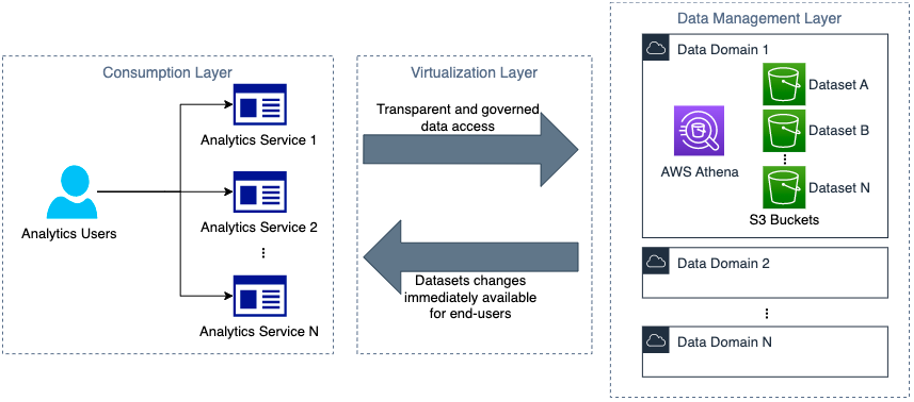
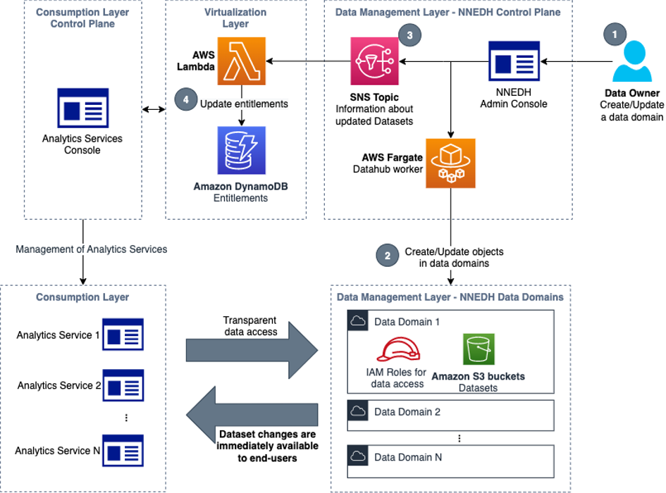
From the end-user perspective, the objective of the mechanisms described in this post is to enable simplified data access from the different analytics services adopted by Novo Nordisk, such as those provided by software as a service (SaaS) vendors like Databricks, or self-hosted ones such as JupyterHub. At the same time, the platform must guarantee that any change in a dataset is immediately reflected at the service user interface. The following figure illustrates at a high level the expected behavior.

High-level data platform expected behavior

Following the layer nomenclature established in the first post, the services are created and managed in the consumption layer. The domain accounts are created and managed in the data management layer. Because changes can occur from both layers, continuous communication in both directions is required. The state information is kept in the virtualization layer along with the communication protocols. Additionally, at sign-in time, the services need information about data resources required to provide data access abstraction.

Managing data access

The data access control in this architecture is designed around the core principle that all access is encapsulated in isolated IAM role sessions. The layer pattern that we described in the first post ensures that the creation and curation of the IAM role policies involved can be delegated to the different data management ecosystems. Each data management platform integrated can use their own data access mechanisms, with the unique requirement that the data is accessed via specific IAM roles.

To illustrate the potential mechanisms that can be used by data management solutions, we show two examples of data access permission mechanisms used by two different data management solutions. Both systems utilize the same trust policies as described in the following sections, but have a completely different permission space.

Example 1: Identity-based ABAC policies

The first mechanism we discuss is an ABAC role that provides access to a home-like data storage area, where users can share within their departments and with the wider organization in a structure that mimics the organizational structure. Here, we don’t utilize the group names, but instead forward user attributes from the corporate Active Directory directly into the permission policy through claim overrides. We do this by having the corporate Active Directory as the identity provider (IdP) for the Amazon Cognito user pool and mapping the relevant IdP attributes to user pool attributes. Then, in the Amazon Cognito identity pool, we map the user pool attributes to session tags to use them for access control. Custom overrides can be included in the claim mapping, through the use of a pre token generation Lambda trigger. This way, claims from AD can be mapped to Amazon Cognito user pool attributes and then ultimately used in the Amazon Cognito identity pool to control IAM role permissions. The following is an example of an IAM policy with sessions tags:

{
    "Version": "2012-10-17",
    "Statement": [
        {
            "Condition": {
                "StringLike": {
                    "s3:prefix": [
                        "",
                        "public/",
                        "public/*",
                        "home/",
                        "home/${aws:PrincipalTag/initials}/*",
                        "home/${aws:PrincipalTag/department}/*"
                    ]
                }
            },
            "Action": "s3:ListBucket",
            "Resource": [
                "arn:aws:s3:::your-home-bucket"
            ],
            "Effect": "Allow"
        },
        {
            "Action": [
                "s3:GetObject*",
                "s3:PutObject*",
                "s3:DeleteObject*"
            ],
            "Resource": [
                "arn:aws:s3:::your-home-bucket/home/${aws:PrincipalTag/initials}",
                "arn:aws:s3:::your-home-bucket/home/${aws:PrincipalTag/initials}/*",
                "arn:aws:s3:::your-home-bucket/public/${aws:PrincipalTag/initials}",
                "arn:aws:s3:::your-home-bucket/public/${aws:PrincipalTag/initials}/*",
                "arn:aws:s3:::your-home-bucket/home/${aws:PrincipalTag/department}",
                "arn:aws:s3:::your-home-bucket/home/${aws:PrincipalTag/department}/*",
                "arn:aws:s3:::your-home-bucket/public/${aws:PrincipalTag/department}",
                "arn:aws:s3:::your-home-bucket/public/${aws:PrincipalTag/department}/*"
            ],
            "Effect": "Allow"
        },
        {
            "Action": "s3:GetObject*",
            "Resource": [
                "arn:aws:s3:::your-home-bucket/public/",
                "arn:aws:s3:::your-home-bucket/public/*"
            ],
            "Effect": "Allow"
        }
    ]
}

This role is then embedded in the analytics layer (together with the data domain roles) and assumed on behalf of the user. This enables users to mix and match between data domains—as well as utilizing private and public data paths that aren’t necessarily tied to any data domain. For more examples of how ABAC can be used with permission policies, refer to How to scale your authorization needs by using attribute-based access control with S3.

Example 2: Lake Formation name-based access controls

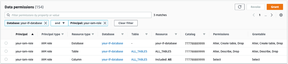
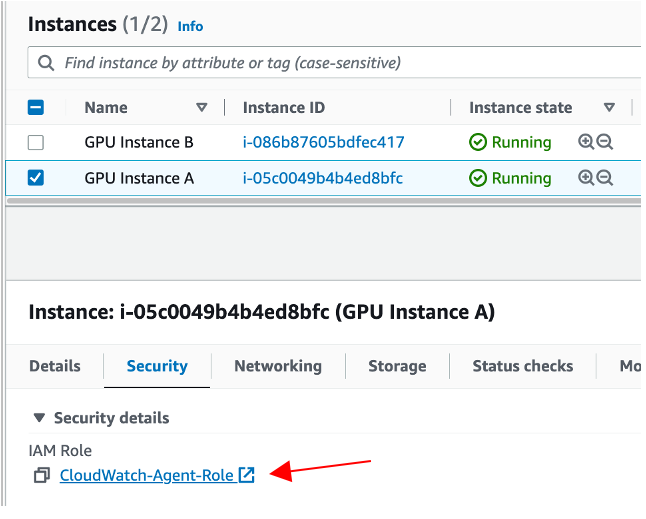
In the data management solution named Novo Nordisk Enterprise Datahub (NNEDH), which we introduced in the first post, we use Lake Formation to enable standardized data access. The NNEDH datasets are registered in the Lake Formation Data Catalog as databases and tables, and permissions are granted using the named resource method. The following screenshot shows an example of these permissions.

Lakeformation named resource method for permissions management

In this approach, data access governance is delegated to Lake Formation. Every data domain in NNEDH has isolated permissions synthesized by NNEDH as the central governance management layer. This is a similar pattern to what is adopted for other domain-oriented data management solutions. Refer to Use an event-driven architecture to build a data mesh on AWS for an example of tag-based access control in Lake Formation.

These patterns don’t exclude implementations of peer-to-peer type data sharing mechanisms, such as those that can be achieved using AWS Resource Access Manager (AWS RAM), where a single IAM role session can have permissions that span across accounts.

Delegating role access to the consumption later

The following figure illustrates the data access workflow from an external service.

Data access workflow from external service

The workflow steps are as follows:

  1. A user authenticates on an IdP used by the analytics tool that they are trying to access. A wide range of analytics tools are supported by Novo Nordisk platform, such as Databricks and JupyterHub, and the IdP can be either SAML or OIDC type depending on the capabilities of the third-party tool. In this example, an Okta SAML application is used to sign into a third-party analytics tool, and an IAM SAML IdP is configured in the data domain AWS account to federate with the external IdP. The third post of this series describes how to set up an Okta SAML application for IAM role federation on Athena.
  2. The SAML assertion obtained during the sign-in process is used to request temporary security credentials of an IAM role through the AssumeRole operation. In this example, the SAML assertion is used onAssumeRoleWithSAMLoperation. For OpenID Connect-compatible IdPs, the operationAssumeRoleWithWebIdentitymust be used with the JWT. The SAML attributes in the assertion or the claims in the token can be generated at sign-in time, to ensure that the group memberships are forwarded, for the ABAC policy pattern described in the following sections.
  3. The analytics tool, such as Databricks or JupyterHub, abstracts the usage of the IAM role session credentials in the tool itself, and data can be accessed directly according to the permissions of the IAM role assumed. This pattern is similar in nature to IAM passthrough as implemented by Databricks, but in Novo Nordisk it’s extended across all analytics services. In this example, the analytics tool accesses the data lake on Amazon Simple Storage Service (Amazon S3) through Athena queries.

As the data mesh pattern expands across domains covering more downstream services, we need a mechanism to keep IdPs and IAM role trusts continuously updated. We come back to this part later in the post, but first we explain how role access is managed at scale.

Attribute-based trust policies

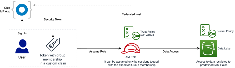
In previous sections, we emphasized that this architecture relies on IAM roles for data access control. Each data management platform can implement its own data access control method using IAM roles, such as identity-based policies or Lake Formation access control. For data consumption, it’s crucial that these IAM roles are only assumable by users that are part of Active Directory groups with the appropriate entitlements to use the role. To implement this at scale, the IAM role’s trust policy uses ABAC.

When a user authenticates on the external IdP of the consumption layer, we add in the access token a claim derived from their Active Directory groups. This claim is propagated by theAssumeRoleoperation into the trust policy of the IAM role, where it is compared with the expected Active Directory group. Only users that belong to the expected groups can assume the role. This mechanism is illustrated in the following figure.

Architecture of the integration with the identity provider

Translating group membership to attributes

To enforce the group membership entitlement at the role assumption level, we need a way to compare the required group membership with the group memberships that a user comes with in their IAM role session. To achieve this, we use a form of ABAC, where we have a way to represent the sum of context-relevant group memberships in a single attribute. A single IAM role session tag value is limited to 256 characters. The corresponding limit for SAML assertions is 100,000 characters, so for systems where a very large number of either roles or group-type mappings are required, SAML can support a wider range of configurations.

In our case, we have opted for a compression algorithm that takes a group name and compresses it to a 4-character string hash. This means that, together with a group-separation character, we can fit 51 groups in a single attribute. This gets pushed down to approximately 20 groups for OIDC type role assumption due to the PackedPolicySize, but is higher for a SAML-based flow. This has shown to be sufficient for our case. There is a risk that two different groups could hash to the same character combination; however, we have checked that there are no collisions in the existing groups. To mitigate this risk going forward, we have introduced guardrails in multiples places. First, before adding new groups entitlements in the virtualization layer, we check if there’s a hash collision with any existing group. When a duplicated group is attempted to be added, our service team is notified and we can react accordingly. But as stated earlier, there is a low probability of clashes, so the flexibility this provides outweighs the overhead associated with managing clashes (we have not had any yet). We additionally enforce this at SAML assertion creation time as well, to ensure that there are no duplicated groups in the users group list, and in cases of duplication, we remove both entirely. This means malicious actors can at most limit the access of other users, but not gain unauthorized access.

Enforcing audit functionality across sessions

As mentioned in the first post, on top of governance, there are strict requirements around auditability of data accesses. This means that for all data access requests, it must be possible to trace the specific user across services and retain this information. We achieve this by setting (and enforcing) a source identity for all role sessions and make sure to propagate enterprise identity to this attribute. We use a combination of Okta inline hooks and SAML session tags to achieve this. This means that the AWS CloudTrail logs for an IAM role session have the following information:

{
    "eventName": "AssumeRoleWithSAML",
    "requestParameters": {
        "SAMLAssertionlD": "id1111111111111111111111111",
        "roleSessionName": "[email protected]",
        "principalTags": {
            "nn-initials": "user",
            "department": "NNDepartment",
            "GroupHash": "xxxx",
            "email": "[email protected]",
            "cost-center": "9999"
        },
        "sourceIdentity": "[email protected]",
        "roleArn": "arn:aws:iam::111111111111:role/your-assumed-role",
        "principalArn": "arn:aws:iam,111111111111:saml-provider/your-saml-provider",
        ...
    },
    ...
}

On the IAM role level, we can enforce the required attribute configuration with the following example trust policy. This is an example for a SAML-based app. We support the same patterns through OpenID Connect IdPs.

We now go through the elements of an IAM role trust policy, based on the following example:

{
    "Version": "2008-10-17",
    "Statement": {
        "Effect": "Allow",
        "Principal": {
            "Federated": [SAML_IdP_ARN]
        },
        "Action": [
            "sts:AssumeRoleWithSAML",
            "sts:TagSession",
            "sts:SetSourceIdentity"
        ],
        "Condition": {
            "StringEquals": {
                "SAML:aud": "https://signin.aws.amazon.com/saml"
            },
            "StringLike": {
                "sts:SourceIdentity": "*@novonordisk.com",
                "aws:RequestTag/GroupHash": ["*xxxx*"]
            },
            "StringNotLike": {
                "sts:SourceIdentity": "*"
            }
        }
    }
}

The policy contains the following details:

  • ThePrincipalstatement should point to the list of apps that are served through the consumption layer. These can be Azure app registrations, Okta apps, or Amazon Cognito app clients. This means that SAML assertions (in the case of SAML-based flows) minted from these applications can be used to run the operationAssumeRoleWithSamlif the remaining elements are also satisfied.
  • TheActionstatement includes the required permissions for theAssumeRolecall to succeed, including adding the contextual information to the role session.
  • In the first condition, the audience of the assertion needs to be targeting AWS.
  • In the second condition, there are twoStringLikerequirements:
    • A requirement on the source identity as the naming convention to follow at Novo Nordisk (users must come with enterprise identity, following our audit requirements).
    • Theaws:RequestTag/GroupHashneeds to bexxxx, which represents the hashed group name mentioned in the upper section.
  • Lastly, we enforce that sessions can’t be started without setting the source identity.

This policy enforces that all calls are from recognized services, include auditability, have the right target, and enforces that the user has the right group memberships.

Building a central overview of governance and trust

In this section, we discuss how Novo Nordisk keeps track of the relevant group-role relations and maps these at sign-in time.

Entitlements

In Novo Nordisk, all accesses are based on Active Directory group memberships. There is no user-based access. Because this pattern is so central, we have extended this access philosophy into our data accesses. As mentioned earlier, at sign-in time, the hooks need to be able to know which roles to assume for a given user, given this user’s group membership. We have modeled this data in Amazon DynamoDB, where just-in-time provisioning ensures that only the required user group memberships are available. By building our application around the use of groups, and by having the group propagation done by the application code, we avoid having to make a more general Active Directory integration, which would, for a company the size of Novo Nordisk, severely impact the application, simply due to the volume of users and groups.

The DynamoDB entitlement table contains all relevant information for all roles and services, including role ARNs and IdP ARNs. This means that when users log in to their analytics services, the sign-in hook can construct the required information for the Roles SAML attribute.

When new data domains are added to the data management layer, the data management layer needs to communicate both the role information and the group name that gives access to the role.

Single sign-on hub for analytics services

When scaling this permission model and data management pattern to a large enterprise such as Novo Nordisk, we ended up creating a large number of IAM roles distributed across different accounts. Then, a solution is required to map and provide access for end-users to the required IAM role. To simplify user access to multiple data sources and analytics tools, Novo Nordisk developed a single sign-on hub for analytics services. From the end-user perspective, this is a web interface that glues together different offerings in a unified system, making it a one-stop tool for data and analytics needs. When signing in to each of the analytical offerings, the authenticated sessions are forwarded, so users never have to reauthenticate.

Common for all the services supported in the consumption layer is that we can run a piece of application code at sign-in time, allowing sign-in time permissions to be calculated. The hooks that achieve this functionality can, for instance, be run by Okta inline hooks. This means that each of the target analytics services can have custom code to translate relevant contextual information or provide other types of automations for the role forwarding.

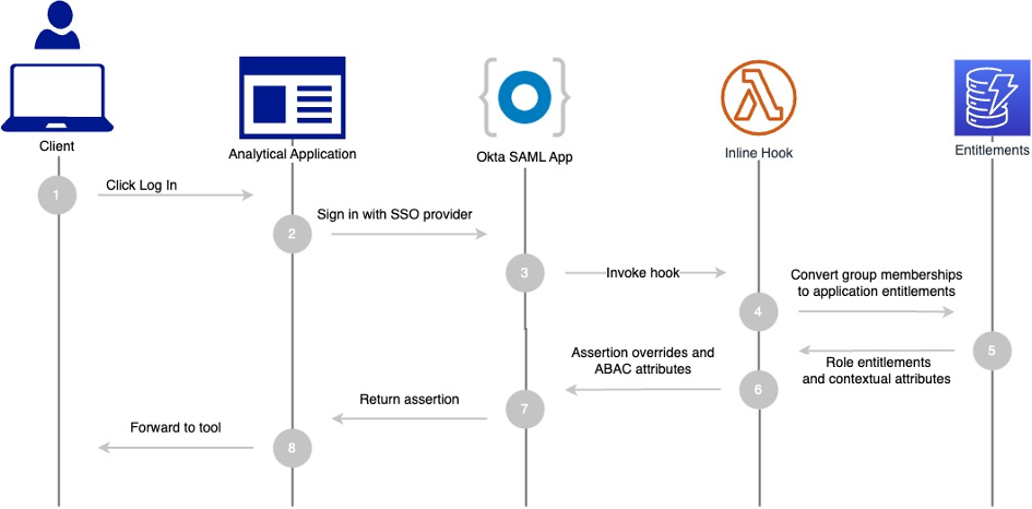
The sign-in flow is demonstrated in the following figure.

Sign-in flow

The workflow steps are as follows:

  1. A user accesses an analytical service such as Databricks in the Novo Nordisk analytics hub.
  2. The service uses Okta as the SAML-based IdP.
  3. Okta invokes an AWS Lambda-based SAML assertion inline hook.
  4. The hook uses the entitlement database, converting application-relevant group memberships into role entitlements.
  5. Relevant contextual information is returned from the entitlement database.
  6. The Lambda-based hook adds new SAML attributes to the SAML assertion, including the hashed group memberships and other contextual information such as source identity.
  7. A modified SAML assertion is used to sign users in to the analytical service.
  8. The user can now use the analytical tool with active IAM role sessions.

Synchronizing role trust

The preceding section gives an overview of how federation works in this solution. Now we can go through how we ensure that all participating AWS environments and accounts are in sync with the latest configuration.

From the end-user perspective, the synchronization mechanism must ensure that every analytics service instantiated can access the data domains assigned to the groups that the user belongs to. Also, changes in data domains—such as granting data access to an Active Directory group—must be effective immediately to every analytics service.

Two event-based mechanisms are used to maintain all the layers synchronized, as detailed in this section.

Synchronize data access control on the data management layer with changes to services in the consumption layer

As describe in the previous section, the IAM roles used for data access are created and managed by the data management layer. These IAM roles have a trust policy providing federated access to the external IdPs used by the analytics tools of the consumption layer. It implies that for every new analytical service created with a different IDP, the IAM roles used for data access on data domains must be updated to trust this new IdP.

Using NNEDH as an example of a data management solution, the synchronization mechanism is demonstrated in the following figure.

Synchronization mechanism in a data management solution

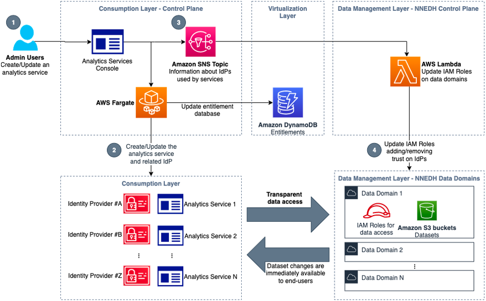
Taking as an example a scenario where a new analytics service is created, the steps in this workflow are as follows:

  1. A user with access to the administration console of the consumption layer instantiates a new analytics service, such as JupyterHub.
  2. A job running on AWS Fargate creates the resources needed for this new analytics service, such as an Amazon Elastic Compute Cloud (Amazon EC2) instance for JupyterHub, and the IdP required, such as a new SAML IdP.
  3. When the IdP is created in the previous step, an event is added in an Amazon Simple Notification Service (Amazon SNS) topic with its details, such as name and SAML metadata.
  4. In the NNEDH control plane, a Lambda job is triggered by new events on this SNS topic. This job creates the IAM IdP, if needed, and updates the trust policy of the required IAM roles in all the AWS accounts used as data domains, adding the trust on the IdP used by the new analytics service.

In this architecture, all the update steps are event-triggered and scalable. This means that users of new analytics services can access their datasets almost instantaneously when they are created. In the same way, when a service is removed, the federation to the IdP is automatically removed if not used by other services.

Propagate changes on data domains to analytics services

Changes to data domains, such as the creation of a new S3 bucket used as a dataset, or adding or removing data access to a group, must be reflected immediately on analytics services of the consumption layer. To accomplish it, a mechanism is used to synchronize the entitlement database with the relevant changes made in NNEDH. This flow is demonstrated in the following figure.

Changes propagation flow

Taking as an example a scenario where access to a specific dataset is granted to a new group, the steps in this workflow are as follows:

  1. Using the NNEDH admin console, a data owner approves a dataset sharing request that grants access on a dataset to an Active Directory group.
  2. In the AWS account of the related data domain, the dataset components such as the S3 bucket and Lake Formation are updated to provide data access to the new group. The cross-account data sharing in Lake Formation uses AWS RAM.
  3. An event is added in an SNS topic with the current details about this dataset, such as the location of the S3 bucket and the groups that currently have access to it.
  4. In the virtualization layer, the updated information from the data management layer is used to update the entitlement database in DynamoDB.

These steps make sure that changes on data domains are automatically and immediately reflected on the entitlement database, which is used to provide data access to all the analytics services of the consumption layer.

Limitations

Many of these patterns rely on the analytical tool to support a clever use of IAM roles. When this is not the case, the platform teams themselves need to develop custom functionality at the host level to ensure that role accesses are correctly controlled. This, for example, includes writing custom authenticators for JupyterHub.

Conclusion

This post shows an approach to building a scalable and secure data and analytics platform. It showcases some of the mechanisms used at Novo Nordisk and how to strike the right balance between freedom and control. The architecture laid out in the first post in this series enables layer independence, and exposes some extremely useful primitives for data access and governance. We make heavy use of contextual attributes to modulate role permissions at the session level, which provide just-in-time permissions. These permissions are propagated at a scale, across data domains. The upside is that a lot of the complexity related to managing data access permission can be delegated to the relevant business groups, while enabling the end-user consumers of data to think as little as possible about data accesses and focus on providing value for the business use cases. In the case of Novo Nordisk, they can provide better outcomes for patients and acceleration innovation.

The next post in this series describes how end-users can consume data from their analytics tool of choice, aligned with the data access controls detailed in this post.


About the Authors

Jonatan Selsing is former research scientist with a PhD in astrophysics that has turned to the cloud. He is currently the Lead Cloud Engineer at Novo Nordisk, where he enables data and analytics workloads at scale. With an emphasis on reducing the total cost of ownership of cloud-based workloads, while giving full benefit of the advantages of cloud, he designs, builds, and maintains solutions that enable research for future medicines.

Hassen Riahi is a Sr. Data Architect at AWS Professional Services. He holds a PhD in Mathematics & Computer Science on large-scale data management. He works with AWS customers on building data-driven solutions.

Alessandro Fior is a Sr. Data Architect at AWS Professional Services. He is passionate about designing and building modern and scalable data platforms that accelerate companies to extract value from their data.

Moses Arthur comes from a mathematics and computational research background and holds a PhD in Computational Intelligence specialized in Graph Mining. He is currently a Cloud Product Engineer at Novo Nordisk, building GxP-compliant enterprise data lakes and analytics platforms for Novo Nordisk global factories producing digitalized medical products.

Anwar RizalAnwar Rizal is a Senior Machine Learning consultant based in Paris. He works with AWS customers to develop data and AI solutions to sustainably grow their business.

Kumari RamarKumari Ramar is an Agile certified and PMP certified Senior Engagement Manager at AWS Professional Services. She delivers data and AI/ML solutions that speed up cross-system analytics and machine learning models, which enable enterprises to make data-driven decisions and drive new innovations.

Optimizing data with automated intelligent document processing solutions

Post Syndicated from Deependra Shekhawat original https://aws.amazon.com/blogs/architecture/optimizing-data-with-automated-intelligent-document-processing-solutions/

Many organizations struggle to effectively manage and derive insights from the large amount of unstructured data locked in emails, PDFs, images, scanned documents, and more. The variety of formats, document layouts, and text makes it difficult for any standard Optical Character Recognition (OCR) to extract key insights from these data sources.

To help organizations overcome these document management and information extraction challenges, AWS offers connected, pre-trained artificial intelligence (AI) service APIs that help drive business outcomes from these document-based rich data sources.

This blog post describes a cost-effective, scalable automated intelligent document processing solution that leverages a Natural Processing Language (NLP) engine using Amazon Textract and Amazon Comprehend. This solution helps customers take advantage of industry leading machine learning (ML) technology in their document workflows without the need for in-house ML expertise.

Customer document management challenges

Customers across industry verticals experience the following document management challenges:

  • Extraction process accuracy varies significantly when applied to diverse sources; specifically handwritten text, images, and scanned documents.
  • Existing scripting and rule-based solutions cannot provide customer domain or problem-specific classifiers.
  • Traditional document management systems cannot consider feedback from domain experts to improve the learning process.
  • The Personally Identifiable Information (PII) data-handling is not robust or customizable, causing data privacy leakage concern.
  • Many manual interventions are required to complete the entire process.

Automated intelligent document processing solution

We introduced an automated intelligent document processing implementation to address key document management challenges. At the heart of the solution is a NLP engine that combines:

The full solution also leverages other AWS services as described in the following diagram (Figure 1) and steps to develop and operate a cost-effective and scalable architecture for document processing. It effectively extracts text from document types including PDFs, images, scanned documents, Microsoft Excel workbooks, and more.

AI-based intelligent document processing engine

Figure 1: AI-based intelligent document processing engine

Solution overview

Let’s explore the automated intelligent document processing solution step by step.

  1. The document upload engine or business users upload the respective files or documents through a custom web application to the designated Amazon Simple Storage Service (Amazon S3) bucket.
  2. The event-based architecture signals an Amazon S3 push event to invoke the respective AWS Lambda function to start document pre-processing.
  3. The Lambda function evaluates the document payload, leverages Amazon Simple Queue Service (Amazon SQS) for async processing, prepares document metadata, stores it in Amazon DynamoDB, and calls the NLP engine to perform the information extraction process.
  4. The NLP engine leverages Amazon Textract for text extraction from a variety of sources and leverages document metadata to optimize the appropriate API calls (for example, form, tabular, or PDF).
    • Amazon Textract output is fed into Amazon Comprehend which consumes the extracted text and performs entity parsing, line/paragraph-based sentiment analysis, and document/paragraph classification. For better accuracy, we leverage a custom classifier within Amazon Comprehend.
    • Amazon Comprehend also provides key APIs to mask PII data before it is used for any further consumption. The solution offers the ability to configure masking rules for each PII entity per masking requirements.
    • To ensure the solution has capability to handle data from Microsoft Excel workbooks, we developed a custom parser using Python running inside an AWS Lambda function. Depending on the document metadata, this function can be invoked.
  5. Output of Amazon Comprehend is then fed to ML models deployed using Amazon SageMaker depending on additional use cases configured by the customer to complement the overall process with ML-based recommendations, predictions, and personalization.
  6. Once the NLP engine completes its processing, the job completion notification event signals another AWS Lambda function and updates the status in the respective Amazon SQS queue.
  7. The Lambda post-processing function parses the resultant content generated by the NLP engine and stores it in the Amazon DynamoDB and Amazon S3 bucket. This step is responsible for the required data augmentation, key entities validation, and default value assignment to create a data structure that could be consumed by the presentation/visualization layer.
  8. Users get the flexibility to see the extracted information and compare it with the original document extract in the custom user interface (UI). They can provide their feedback on extraction and entity parsing accuracy. From a user access management perspective, Amazon Cognito provides authorization and authentication.

Customer benefits

The automated intelligent document processing solution helps customers:

  • Increase overall document management efficiency by 50-60%, leveraging automation and nullifying manual interventions
  • Reduce in-house team involvement in administrative activities by up to 70% using integrated and connected processing workflows
  • Gain better visibility into key contractual obligations with features such as Document Classification (helps properly route documents to the respective process/team) and Obligation Extraction
  • Utilize a UI-based feedback mechanism for in-house domain experts/reviewers to see and validate the extracted information and offer feedback to inform further model training

From a cost-optimization perspective, depending on document type and required information, only the respective Amazon Textract APIs calls are submitted. (For example, it is not worth using form/table-based Textract API calls for a Know Your Customer (KYC) document such as a driver’s license or passport when the AnalyzeID API is the most efficient solution.)

To maximize solution benefits, customers should invest time in building well-defined taxonomies ahead of using the document processing solution to accommodate their own use cases or industry domain-specific requirements. Their taxonomy input highlights only relevant keys and takes respective actions in case the requires keys are not extracted.

Vertical industry use cases

As mentioned, this document processing solution can be used across industry segments. Let’s explore some practical use cases. For example, it can help insurance industry professionals to accelerate claim processing and customer KYC-related processes. By extracting the key entities from the claim documents, mapping them against the customer defined taxonomy, and integrating with Amazon SageMaker models for anomaly detection (anomalous claims), insurance providers can improve claim management and customer satisfaction.

In the healthcare industry, the solution can help with medical records and report processing, key medical entity extraction, and customer data masking.

The document processing solution can help the banking industry by automating check processing and delivering the ability to extract key entities like payer, payee, date, and amount from the checks.

Conclusion

Manual document processing is resource-intensive, time consuming, and costly. Customers need to allocate resources to process large volume documents, lowering business agility. Their employees are performing manual “stare and compare” tasks, potentially reducing worker morale and preventing them from focusing where their efforts are better placed.

Intelligent document processing helps businesses overcome these challenges by automating the classification, extraction, and analysis of data. This expedites decision cycles, allocates resources to high-value tasks, and reduces costs.

Pre-trained APIs of AWS AI services allow for quick classification, extraction, and data analyzation from scores of documents. This solution also has industry specific features that can quickly process specialized industry specific documents. This blog discussed the foundational architecture to helps to accelerate implementation of any specific document processing use case.

How CyberCRX cut ML processing time from 8 days to 56 minutes with AWS Step Functions Distributed Map

Post Syndicated from Marcia Villalba original https://aws.amazon.com/blogs/aws/how-cybercrx-cut-ml-processing-time-from-8-days-to-56-minutes-with-aws-step-functions-distributed-map/

Last December, Sébastien Stormacq wrote about the availability of a distributed map state for AWS Step Functions, a new feature that allows you to orchestrate large-scale parallel workloads in the cloud. That’s when Charles Burton, a data systems engineer for a company called CyberGRX, found out about it and refactored his workflow, reducing the processing time for his machine learning (ML) processing job from 8 days to 56 minutes. Before, running the job required an engineer to constantly monitor it; now, it runs in less than an hour with no support needed. In addition, the new implementation with AWS Step Functions Distributed Map costs less than what it did originally.

What CyberGRX achieved with this solution is a perfect example of what serverless technologies embrace: letting the cloud do as much of the undifferentiated heavy lifting as possible so the engineers and data scientists have more time to focus on what’s important for the business. In this case, that means continuing to improve the model and the processes for one of the key offerings from CyberGRX, a cyber risk assessment of third parties using ML insights from its large and growing database.

What’s the business challenge?
CyberGRX shares third-party cyber risk (TPCRM) data with their customers. They predict, with high confidence, how a third-party company will respond to a risk assessment questionnaire. To do this, they have to run their predictive model on every company in their platform; they currently have predictive data on more than 225,000 companies. Whenever there’s a new company or the data changes for a company, they regenerate their predictive model by processing their entire dataset. Over time, CyberGRX data scientists improve the model or add new features to it, which also requires the model to be regenerated.

The challenge is running this job for 225,000 companies in a timely manner, with as few hands-on resources as possible. The job runs a set of operations for each company, and every company calculation is independent of other companies. This means that in the ideal case, every company can be processed at the same time. However, implementing such a massive parallelization is a challenging problem to solve.

First iteration
With that in mind, the company built their first iteration of the pipeline using Kubernetes and Argo Workflows, an open-source container-native workflow engine for orchestrating parallel jobs on Kubernetes. These were tools they were familiar with, as they were already using them in their infrastructure.

But as soon as they tried to run the job for all the companies on the platform, they ran up against the limits of what their system could handle efficiently. Because the solution depended on a centralized controller, Argo Workflows, it was not robust, and the controller was scaled to its maximum capacity during this time. At that time, they only had 150,000 companies. And running the job with all of the companies took around 8 days, during which the system would crash and need to be restarted. It was very labor intensive, and it always required an engineer on call to monitor and troubleshoot the job.

The tipping point came when Charles joined the Analytics team at the beginning of 2022. One of his first tasks was to do a full model run on approximately 170,000 companies at that time. The model run lasted the whole week and ended at 2:00 AM on a Sunday. That’s when he decided their system needed to evolve.

Second iteration
With the pain of the last time he ran the model fresh in his mind, Charles thought through how he could rewrite the workflow. His first thought was to use AWS Lambda and SQS, but he realized that he needed an orchestrator in that solution. That’s why he chose Step Functions, a serverless service that helps you automate processes, orchestrate microservices, and create data and ML pipelines; plus, it scales as needed.

Charles got the new version of the workflow with Step Functions working in about 2 weeks. The first step he took was adapting his existing Docker image to run in Lambda using Lambda’s container image packaging format. Because the container already worked for his data processing tasks, this update was simple. He scheduled Lambda provisioned concurrency to make sure that all functions he needed were ready when he started the job. He also configured reserved concurrency to make sure that Lambda would be able to handle this maximum number of concurrent executions at a time. In order to support so many functions executing at the same time, he raised the concurrent execution quota for Lambda per account.

And to make sure that the steps were run in parallel, he used Step Functions and the map state. The map state allowed Charles to run a set of workflow steps for each item in a dataset. The iterations run in parallel. Because Step Functions map state offers 40 concurrent executions and CyberGRX needed more parallelization, they created a solution that launched multiple state machines in parallel; in this way, they were able to iterate fast across all the companies. Creating this complex solution, required a preprocessor that handled the heuristics of the concurrency of the system and split the input data across multiple state machines.

This second iteration was already better than the first one, as now it was able to finish the execution with no problems, and it could iterate over 200,000 companies in 90 minutes. However, the preprocessor was a very complex part of the system, and it was hitting the limits of the Lambda and Step Functions APIs due to the amount of parallelization.

Second iteration with AWS Step Functions

Third and final iteration
Then, during AWS re:Invent 2022, AWS announced a distributed map for Step Functions, a new type of map state that allows you to write Step Functions to coordinate large-scale parallel workloads. Using this new feature, you can easily iterate over millions of objects stored in Amazon Simple Storage Service (Amazon S3), and then the distributed map can launch up to 10,000 parallel sub-workflows to process the data.

When Charles read in the News Blog article about the 10,000 parallel workflow executions, he immediately thought about trying this new state. In a couple of weeks, Charles built the new iteration of the workflow.

Because the distributed map state split the input into different processors and handled the concurrency of the different executions, Charles was able to drop the complex preprocessor code.

The new process was the simplest that it’s ever been; now whenever they want to run the job, they just upload a file to Amazon S3 with the input data. This action triggers an Amazon EventBridge rule that targets the state machine with the distributed map. The state machine then executes with that file as an input and publishes the results to an Amazon Simple Notification Service (Amazon SNS) topic.

Final iteration with AWS Step Functions

What was the impact?
A few weeks after completing the third iteration, they had to run the job on all 227,000 companies in their platform. When the job finished, Charles’ team was blown away; the whole process took only 56 minutes to complete. They estimated that during those 56 minutes, the job ran more than 57 billion calculations.

Processing of the Distributed Map State

The following image shows an Amazon CloudWatch graph of the concurrent executions for one Lambda function during the time that the workflow was running. There are almost 10,000 functions running in parallel during this time.

Lambda concurrency CloudWatch graph

Simplifying and shortening the time to run the job opens a lot of possibilities for CyberGRX and the data science team. The benefits started right away the moment one of the data scientists wanted to run the job to test some improvements they had made for the model. They were able to run it independently without requiring an engineer to help them.

And, because the predictive model itself is one of the key offerings from CyberGRX, the company now has a more competitive product since the predictive analysis can be refined on a daily basis.

Learn more about using AWS Step Functions:

You can also check the Serverless Workflows Collection that we have available in Serverless Land for you to test and learn more about this new capability.

Marcia

Best Practices for managing data residency in AWS Local Zones using landing zone controls

Post Syndicated from Sheila Busser original https://aws.amazon.com/blogs/compute/best-practices-for-managing-data-residency-in-aws-local-zones-using-landing-zone-controls/

This blog post is written by Abeer Naffa’, Sr. Solutions Architect, Solutions Builder AWS, David Filiatrault, Principal Security Consultant, and Jared Thompson Hybrid Edge SA Specialist.

In this post, we discuss how you can leverage AWS Control Tower landing zone and AWS Organizations custom policies – guardrails – at the root level, known as Service Control Policies (SCPS) to enable certain data residency requirements on AWS Local Zones. Using the suggested controls lets you limit the ability to store data, process data outside a geographic location, and keep your data within specific Local Zone(s).

Data residency is a critical consideration for organizations that collect and store sensitive information, such as Personal Identifiable Information (PII), financial data, and healthcare data. With the rise of cloud computing and the global nature of the Internet, it can be challenging for organizations to make sure that their data is being stored and processed in compliance with local laws and regulations.

One potential solution for addressing data residency challenges with AWS is utilizing Local Zones, which places AWS infrastructure in large metro areas. This enables organizations to store and process data in specific geographic locations. By using Local Zones, organizations can architect their environment to meet data residency requirements when an AWS Region is unavailable within the same legal jurisdiction. Local Zones can be configured to utilize landing zone to further adhere to data residency requirements.

A landing zone is a well-architected, multi-account AWS environment that is scalable and secure. This is a starting point from which your organization can quickly launch and deploy workloads and applications with confidence in your security and infrastructure environment.

When leveraging a Local Zone to meet data residency requirements, you must have control over the in-scope data movement from the Local Zones to the AWS Region. This can be accomplished by implementing landing zone best practices and the suggested guardrails. The main focus of this post is the custom policies that restrict data snapshots, prohibit data creation within the Region, and limit data transfer to the Region. Furthermore, this post covers which prerequisites organizations should consider before implementing these guardrails.

Prerequisites

Landing zones best practices and custom guardrails can help when data must remain in a specific locality where the Local Zone is also located. This can be completed by defining and enforcing policies for data storage and usage within the landing zone organization that you set up. The following prerequisites should be considered before implementing the suggested guardrails:

  1. AWS Local Zones

Local Zones are enabled through the Amazon Elastic Compute Cloud (Amazon EC2) console or the AWS Command Line Interface (AWS CLI).

You can start using available AWS services on the designated Local Zone directly from the console. Moreover, you can manage the Local Zone using the same tools and interfaces that you use in AWS Region.

2. AWS Control Tower landing zone

AWS Control Tower is a managed service that provides a pre-packaged set of best-practice blueprints for setting up and governing multi-account AWS environments. You must have Control Tower fully implemented in your environment before you can deploy custom guardrails.

Control Tower launches a key resource associated with your account, called a landing zone, which serves as a home for your organizations and their accounts.

Note that Control Tower relies on Organizations to create and manage multi-account structures.

  1. Set up the data residency guardrails

Using Organizations, you must make sure that the Local Zone is enabled within a workload account in the landing zones.

Figure 1 Landing Zones Accelerator Local Zones workload on AWS high level Architecture

Figure 1: Landing Zones Accelerator – Local Zones workload on AWS high level Architecture

Utilizing Local Zones for regulated components

The availability of Local Zones provides an excellent opportunity to meet data residency requirements and comply with local regulations that restrict the use of the Region outside of your required geo-political boundary. By leveraging Local Zones, organizations can maintain compliance while utilizing AWS services to support their business needs. AWS owns and manages the infrastructure, including hardware, software, and networking for Local Zones. However, as part of the shared responsibility model, customers are responsible for the security of their applications and data, including access control, data encryption, etc.

You must also comply with all applicable regulations and security standards, such as HIPAA, PCI DSS, and GDPR. You should conduct regular security assessments and implement appropriate security controls to protect their applications and data.

In this post, we consider a scenario where there is a single Local Zones location in a metro. However, you must analyze the specific requirements of your workloads and the relevant regulations that apply to determine the most appropriate high availability configurations for your case.

Local Zones workload data residency guardrails

Organizations provides central governance and management for multiple accounts. Central security administrators use SCPs with Organizations to establish controls to which all AWS Identity and Access Management (IAM) principals (users and roles) adhere.

Now you can use SCPs to set permission guardrails. The suggested preventative controls that leverage the implementation of SCPs for data residency on Local Zones are shown in the next paragraph. SCPs let you set permission guardrails by defining the maximum available permissions for IAM entities in an account and all accounts within the Organization root or Organizational Unit (OU). If an SCP denies an action for an account, then none of the entities in any member account, including the member account’s root user, can take that action, even if their IAM permissions let them. The guardrails set in SCPs apply to all IAM entities in the account, which include all users, roles, and the account root user.

 Upon finalizing these prerequisites, you can create the guardrails for the chosen OU.

Note that although the following guidelines serve as helpful guardrails – SCPs – for data residency, you should consult internally with legal and security teams for specific organizational requirements.

 To exercise better control over the workload in Local Zones and prevent data transfer from Local Zones or data storage outside of the Local Zones, consider implementing the following guardrails:

  1. When your data residency requirements require restricting data transfer/saving to the Region, consider the following guardrails:

a. Deny copying data from Local Zones to the Region for Amazon EC2), Amazon Relational Database Service (Amazon RDS), Amazon ElastiCache, and data sync “DenyCopyToRegion”.

As the available services in Local Zones can vary based on location, you must review the services available in the chosen Local Zone and Adjust the SCPs accordingly.

b. Deny Amazon Simple Storage Service (Amazon S3) put action to the Region “DenyPutObjectToRegionalBuckets”.

If your data residency requirements mandate restrictions on data storage in the Region, then consider implementing this guardrail to prevent the use of Amazon S3 in the Region.

c. If your data residency requirements mandate restrictions on data storage in the Region, then consider implementing “DenyDirectTransferToRegion”

Out of Scope is metadata such as tags or operational data such as AWS Key Management Service (AWS KMS) keys.

{
  "Version": "2012-10-17",
  "Statement": [
      {
      "Sid": "DenyCopyToRegion",
      "Action": [
        "ec2:ModifyImageAttribute",
        "ec2:CopyImage",  
        "ec2:CreateImage",
        "ec2:CreateInstanceExportTask",
        "ec2:ExportImage",
        "ec2:ImportImage",
        "ec2:ImportInstance",
        "ec2:ImportSnapshot",
        "ec2:ImportVolume",
        "rds:CreateDBSnapshot",
        "rds:CreateDBClusterSnapshot",
        "rds:ModifyDBSnapshotAttribute",
        "elasticache:CreateSnapshot",
        "elasticache:CopySnapshot",
        "datasync:Create*",
        "datasync:Update*"
      ],
      "Resource": "*",
      "Effect": "Deny"
    },
    {
      "Sid": "DenyDirectTransferToRegion",
      "Action": [
        "dynamodb:PutItem",
        "dynamodb:CreateTable",
        "ec2:CreateTrafficMirrorTarget",
        "ec2:CreateTrafficMirrorSession",
        "rds:CreateGlobalCluster",
        "es:Create*",
        "elasticfilesystem:C*",
        "elasticfilesystem:Put*",
        "storagegateway:Create*",
        "neptune-db:connect",
        "glue:CreateDevEndpoint",
        "glue:UpdateDevEndpoint",
        "datapipeline:CreatePipeline",
        "datapipeline:PutPipelineDefinition",
        "sagemaker:CreateAutoMLJob",
        "sagemaker:CreateData*",
        "sagemaker:CreateCode*",
        "sagemaker:CreateEndpoint",
        "sagemaker:CreateDomain",
        "sagemaker:CreateEdgePackagingJob",
        "sagemaker:CreateNotebookInstance",
        "sagemaker:CreateProcessingJob",
        "sagemaker:CreateModel*",
        "sagemaker:CreateTra*",
        "sagemaker:Update*",
        "redshift:CreateCluster*",
        "ses:Send*",
        "ses:Create*",
        "sqs:Create*",
        "sqs:Send*",
        "mq:Create*",
        "cloudfront:Create*",
        "cloudfront:Update*",
        "ecr:Put*",
        "ecr:Create*",
        "ecr:Upload*",
        "ram:AcceptResourceShareInvitation"
      ],
      "Resource": "*",
      "Effect": "Deny"
    },
    {
      "Sid": "DenyPutObjectToRegionalBuckets",
      "Action": [
        "s3:PutObject"
      ],
      "Resource": ["arn:aws:s3:::*"],
      "Effect": "Deny"
    }
  ]
}
  1. If your data residency requirements require limitations on data storage in the Region, then consider implementing this guardrail “DenyAllSnapshots” to restrict the use of snapshots in the Region.

Note that the following guardrail restricts the creation of snapshots on AWS Outposts as well. If you’re using Outposts in the same AWS account, then you may need to customize this guardrail to make sure that it aligns with your organization’s specific needs and requirements. For more information on data residency considerations for Outposts, please refer to Architecting for data residency with AWS Outposts rack and landing zone guardrails.

{
  "Version": "2012-10-17",
  "Statement": [

    {
      "Sid": "DenyAllSnapshots",
      "Effect":"Deny",
      "Action":[
        "ec2:CreateSnapshot",
        "ec2:CreateSnapshots",
        "ec2:CopySnapshot",
        "ec2:ModifySnapshotAttribute"
      ],
      "Resource":"arn:aws:ec2:*::snapshot/*"
    }
  ]
}
  1. This guardrail helps prevent the launch of EC2 instances or the creation of network interfaces by subnet as opposed to Local Zones You should keep data residency workloads within the Local Zones rather than the Region to make sure of better control over regulated workloads. This approach can help your organization achieve better control over data residency workloads and improve governance over your Organization.

 Make sure to update the Local Zones subnets < localzones_subnet_arns>.

{
"Version": "2012-10-17",
  "Statement":[{
    "Sid": "DenyNotLocalZonesSubnet",
    "Effect":"Deny",
    "Action": [
      "ec2:RunInstances",
      "ec2:CreateNetworkInterface"
    ],
    "Resource": [
      "arn:aws:ec2:*:*:network-interface/*"
    ],
    "Condition": {
      "ForAllValues:ArnNotEquals": {
        "ec2:Subnet": ["<localzones_subnet_arns>"]
      }
    }
  }]
}

Additional considerations

When implementing data residency guardrails on Local Zones, consider backup and disaster recovery strategies to make sure that your data is protected in the event of an outage or other unexpected events. This may include creating regular backups of your data, implementing disaster recovery plans and procedures, and using redundancy and failover systems to minimize the impact of any potential disruptions. Additionally, you should make sure that your backup and disaster recovery systems are compliant with any relevant data residency regulations and requirements. You should also test your backup and disaster recovery systems regularly to make sure that they are functioning as intended.

Additionally, the provided SCPs for Local Zones in the above example do not block the “logs:PutLogEvents”. Therefore, even if you implemented data residency guardrails on Local Zones, the application may log data to Amazon CloudWatch Logs in the Region.

Highlights

By default, application-level logs on Local Zones are not automatically sent to CloudWatch Logs in the Region. You can configure CloudWatch Logs agent on Local Zones to collect and send your application-level logs to CloudWatch Logs.

logs:PutLogEvents does transmit data to the Region, but it is not blocked by the provided SCPs, as it’s expected that most use cases still want to be able to use this logging API. However, if blocking is desired, then add the action to the first recommended guardrail. If you want specific roles to be allowed, then combine with the ArnNotLike condition example referenced in the Customization Guide.

Conclusion

The combined use of Local Zones and the suggested guardrails via Organizations policies enables you to exercise better control over the movement of the data. By creating a landing zone for your organization, you can apply SCPs to your Local Zones that will help make sure that your data remains within a specific geographic location, as required by the data residency regulations.

Note that, although custom guardrails can help you manage data residency on Local Zones, it’s critical to thoroughly review your policies, procedures, and configurations. This lets you make sure that they are compliant with all relevant data residency regulations and requirements. Regularly testing and monitoring your systems can help make sure that your data is protected and your organization stays compliant.

References

Optimizing Amazon EC2 Spot Instances with Spot Placement Scores

Post Syndicated from Sheila Busser original https://aws.amazon.com/blogs/compute/optimizing-amazon-ec2-spot-instances-with-spot-placement-scores/

This blog post is written by Steve Cole, Principal Specialist SA, and Robert McCone, Sr. Specialist SA.

Getting the compute resources you need, even vCPUS numbering in the millions, and completing a workload using Amazon EC2 Spot Instances is just a configuration away. In this post you will learn how to use Spot placement scores to reduce interruptions, acquire greater capacity, and identify optimal configurations, times, and locations to run workloads on Spot Instances. Amazon EC2 Spot Instances let you take advantage of unused EC2 capacity in the AWS cloud and are available at up to a 90% discount compared to On-Demand prices. Spot placement scores is a feature that many customers use to identify optimal instance types or to choose the best Availability Zone (AZ) for ephemeral work like data analytics or high-performance computing. As a real-time tool, Spot placement scores are often integrated into deployment automation. However, because of its logging and graphic capabilities, you may find it be a valuable resource even before you launch a workload into the cloud. Now available through AWS Labs, a Github repository hosting tools for customers, the Spot placement score tracker tackles the undifferentiated heavy lifting and can do this for any customer.

About Spot placement score

Spot placement scores are a feature available through AWS APIs – also implemented in the Amazon EC2 Spot requests console – that uses internal capacity and interruption data to scrutinize the size and shape of a Spot Instance request and responds with a “likelihood of success” rating of 1 to imply lower likelihood of success and 10 to imply higher likelihood of success. The score represents confidence in being able to acquire the desired capacity (size) using the instance configuration (shape) for the next few hours. The shape of the request can be a list of specific instances or can be requirements-based with attribute-based instance type selection. The size of the request can be instance count, number of vCPUs, or GB of RAM. It’s based on known capacity, allocation strategies, and the trending of capacities over time.

Before the release of Spot placement score, customers could track the trends of their existing workloads and configurations. This might have helped them to anticipate capacity constraints over time, but the ability to do something more meaningful when assessing configurations was something customers requested often. With the launch of Spot placement score, that capability was delivered and enabled customers to receive guidance on how a configuration change might affect the effectiveness of Spot Instances in a workload.

Customers immediately recognized the power of this new feature and started writing tooling around their workloads to incorporate the new functionality provided by Spot placement scores. For examples, customers leveraged Spot placement scores to find the highest scoring AZ in a region for work that requires low latency within a cluster. Customers running data analytics with services like Amazon EMR could more confidently launch clusters on Spot Instances. This reduces costs and the time necessary to process data because of fewer interruptions. Financial customers, health care and life sciences, and high tech were some of the early adopters of this strategy.

Benefits of Spot placement scores

One specific customer used tools like the Spot instance advisor and Spot pricing history tools to make decisions about what instances to run every night. If the customer’s analytics workload received too many interruptions, then it would inevitably be relaunched using On-Demand Instances, increasing costs and time-to-complete. The addition of Spot placement scores to the customer’s tooling allowed for more informed decisions about which configurations worked best and, more specifically, which AZ(s) to use. Ultimately, this led not only to higher confidence in using Spot instances, but also to significant cost savings over time.

Other customers tracked Spot placement scores over time with regular queries stored in time series databases to identify not only the best configuration or location, but also the best time-of-day or day-of-week to run their workloads. Different configurations of instance types were queried through automation and the results were logged into a time series database that could then be presented as graphs. These graphs were scrutinized, configurations were tuned, and ultimately these customers could take greater advantage of the cost optimization that Spot instances offer through fewer interruptions by running their workloads where and when scores were higher.

AWS was interested in how this solved problems for customers, and after some more research with customers and design ideation, led to the creation of an OSS tool that AWS has recently released: Spot placement score tracker. Spot placement score tracker helps customers evaluate different configurations against multiple times and locations. It’s an AWS-native solution that leverages the Spot placement score API along with AWS Lambda and Amazon CloudWatch to create a dashboard that enables any AWS customer to benefit from this model without having to write it themselves.

How to use the Spot placement score tracker

The project provides Infrastructure as Code (IaC) automation using the AWS Cloud Development Kit (AWS CDK) to deploy the infrastructure and permissions required to run Lambda. This gets executed every five minutes to collect the placement scores of as many diversified configurations as defined.

Architectural diagram: CDK building connections between EventBridge, Lambda, S3, and CloudWatch to generate dashboards

After installing the CloudWatch dashboard, and given some time to collect and record data, you will be provided valuable insights in an intuitive graph such as those in the following example.

Sample CloudWatch dashboard with four graphs showing Spot placement score results over time for different configurations

Insights available through the Spot placement score tracker

The first thing you may notice by observing data over time is that instance diversification is the primary driver of high placement scores. This has always been a best practice for the use of Spot Instances, and it extends to On-Demand Instances as well. In short, if you can only run on one instance type, then the likelihood of experiencing interruptions is far greater than if you can run on six or twelve. Sometimes the simple inclusion of -a, -d, and -n instance types (e.g. m5.large, m5a.large, m5d.large, m5d.large), previous generations (e.g., m5.large, m4.large), different sizes in a container environment (e.g., m5.large, m5.xlarge, m5.2xlarge), and even the inclusion of AWS Graviton will have a material impact on placement scores, which equates to fewer interruptions. This ultimately leads to more efficient use of resources through less restarted processes, resulting in increased efficiency and reduced costs.

The second insight that you can realize through the use of placement scores over time is identifying the optimal AZ in which an ephemeral process can be placed. Perhaps the best use case for this type of insight is data analytics clusters that are launched to complete many calculations overnight. This is common in financial institutions for various reasons including risk analysis and compliance, but could apply to medical research examining results of experiments during the day as well as other situations where a 24/7 presence isn’t required by the workload. These customers are typically using a single AZ to allow for faster communication between nodes and to reduce data transfer costs. Therefore, the ability for Spot placement scores to provide different scores for different AZs is highly advantageous.

Third, with access to placement scores over time, it becomes possible to identify exactly how large a workload’s footprint can be. By submitting identical configurations to Spot placement scores but with different sizes, you can surface the ideal workload size. Not too small, where perhaps the job takes too long to complete, but also not so large that the interruptions are too frequent and cause restarts too often. This can benefit not only ephemeral workloads, but also persistent clusters or fleets by understanding what the lowest score would be over time and giving you solid information regarding what they can expect from Spot Instances and where. This might inform you to be ready to launch On-Demand Instances to compensate when Spot Instance availability is lower. This can also help to forecast pricing and inform decisions about the consideration of AWS Savings Plans or On-Demand Capacity Reservations.

Finally, analyzing Spot placement scores over time can provide regional scoring. Through this lens it’s possible for you to identify entire regions that they may have overlooked without the knowledge that Spot Instances outside the your primary region(s) might offer lower interruptions during daylight hours due to them being off-peak. When it’s possible to place a workload in another region, unconstrained by local data access requirements, it’s quite possible to harness the compute of a significant footprint in locations that are otherwise un(der)-utilized. Workloads that require less data transfer and more compute can benefit tremendously from access to Spot Instances in other regions. For example, things like build servers might run extraordinarily well in Europe during North American business hours and the reduction in compute cost might offset the data transfer to complete the job.

Conclusion

Spot placement scores can be used to make decisions about how, when, and where Spot Instances can be most efficiently utilized to deliver business needs, and at greatly reduced prices. We’re very excited to release this tool to enable you to tap into information which was previously unavailable and make data-driven decisions for your business. The information in this post, combined with the output of placement scores over time, is a significant evolution.

Install the Spot placement score tracker today, configure it to match an existing Spot workload, and see how you might perform at different times or different locations.  Explore more robust options and discover greater capacity and lower interruptions. Or investigate how On-Demand workloads could migrate to Spot Instances.

How the BMW Group analyses semiconductor demand with AWS Glue

Post Syndicated from Göksel SARIKAYA original https://aws.amazon.com/blogs/big-data/how-the-bmw-group-analyses-semiconductor-demand-with-aws-glue/

This is a guest post co-written by Maik Leuthold and Nick Harmening from BMW Group.

The BMW Group is headquartered in Munich, Germany, where the company oversees 149,000 employees and manufactures cars and motorcycles in over 30 production sites across 15 countries. This multinational production strategy follows an even more international and extensive supplier network.

Like many automobile companies across the world, the BMW Group has been facing challenges in its supply chain due to the worldwide semiconductor shortage. Creating transparency about BMW Group’s current and future demand of semiconductors is one key strategic aspect to resolve shortages together with suppliers and semiconductor manufacturers. The manufacturers need to know BMW Group’s exact current and future semiconductor volume information, which will effectively help steer the available worldwide supply.

The main requirement is to have an automated, transparent, and long-term semiconductor demand forecast. Additionally, this forecasting system needs to provide data enrichment steps including byproducts, serve as the master data around the semiconductor management, and enable further use cases at the BMW Group.

To enable this use case, we used the BMW Group’s cloud-native data platform called the Cloud Data Hub. In 2019, the BMW Group decided to re-architect and move its on-premises data lake to the AWS Cloud to enable data-driven innovation while scaling with the dynamic needs of the organization. The Cloud Data Hub processes and combines anonymized data from vehicle sensors and other sources across the enterprise to make it easily accessible for internal teams creating customer-facing and internal applications. To learn more about the Cloud Data Hub, refer to BMW Group Uses AWS-Based Data Lake to Unlock the Power of Data.

In this post, we share how the BMW Group analyzes semiconductor demand using AWS Glue.

Logic and systems behind the demand forecast

The first step towards the demand forecast is the identification of semiconductor-relevant components of a vehicle type. Each component is described by a unique part number, which serves as a key in all systems to identify this component. A component can be a headlight or a steering wheel, for example.

For historic reasons, the required data for this aggregation step is siloed and represented differently in diverse systems. Because each source system and data type have its own schema and format, it’s particularly difficult to perform analytics based on this data. Some source systems are already available in the Cloud Data Hub (for example, part master data), therefore it’s straightforward to consume from our AWS account. To access the remaining data sources, we need to build specific ingest jobs that read data from the respective system.

The following diagram illustrates the approach.

The data enrichment starts with an Oracle Database (Software Parts) that contains part numbers that are related to software. This can be the control unit of a headlight or a camera system for automated driving. Because semiconductors are the basis for running software, this database builds the foundation of our data processing.

In the next step, we use REST APIs (Part Relations) to enrich the data with further attributes. This includes how parts are related (for example, a specific control unit that will be installed into a headlight) and over which timespan a part number will be built into a vehicle. The knowledge about the part relations is essential to understand how a specific semiconductor, in this case the control unit, is relevant for a more general part, the headlight. The temporal information about the use of part numbers allows us to filter out outdated part numbers, which will not be used in the future and therefore have no relevance in the forecast.

The data (Part Master Data) can directly be consumed from the Cloud Data Hub. This database includes attributes about the status and material types of a part number. This information is required to filter out part numbers that we gathered in the previous steps but have no relevance for semiconductors. With the information that was gathered from the APIs, this data is also queried to extract further part numbers that weren’t ingested in the previous steps.

After data enrichment and filtering, a third-party system reads the filtered part data and enriches the semiconductor information. Subsequently, it adds the volume information of the components. Finally, it provides the overall semiconductor demand forecast centrally to the Cloud Data Hub.

Applied services

Our solution uses the serverless services AWS Glue and Amazon Simple Storage Service (Amazon S3) to run ETL (extract, transform, and load) workflows without managing an infrastructure. It also reduces the costs by paying only for the time jobs are running. The serverless approach fits our workflow’s schedule very well because we run the workload only once a week.

Because we’re using diverse data source systems as well as complex processing and aggregation, it’s important to decouple ETL jobs. This allows us to process each data source independently. We also split the data transformation into several modules (Data Aggregation, Data Filtering, and Data Preparation) to make the system more transparent and easier to maintain. This approach also helps in case of extending or modifying existing jobs.

Although each module is specific to a data source or a particular data transformation, we utilize reusable blocks inside of every job. This allows us to unify each type of operation and simplifies the procedure of adding new data sources and transformation steps in the future.

In our setup, we follow the security best practice of the least privilege principle, to ensure the information is protected from accidental or unnecessary access. Therefore, each module has AWS Identity and Access Management (IAM) roles with only the necessary permissions, namely access to only data sources and buckets the job deals with. For more information regarding security best practices, refer to Security best practices in IAM.

Solution overview

The following diagram shows the overall workflow where several AWS Glue jobs are interacting with each other sequentially.

As we mentioned earlier, we used the Cloud Data Hub, Oracle DB, and other data sources that we communicate with via the REST API. The first step of the solution is the Data Source Ingest module, which ingests the data from different data sources. For that purpose, AWS Glue jobs read information from different data sources and writes into the S3 source buckets. Ingested data is stored in the encrypted buckets, and keys are managed by AWS Key Management Service (AWS KMS).

After the Data Source Ingest step, intermediate jobs aggregate and enrich the tables with other data sources like components version and categories, model manufacture dates, and so on. Then they write them into the intermediate buckets in the Data Aggregation module, creating comprehensive and abundant data representation. Additionally, according to the business logic workflow, the Data Filtering and Data Preparation modules create the final master data table with only actual and production-relevant information.

The AWS Glue workflow manages all these ingestion jobs and filtering jobs end to end. An AWS Glue workflow schedule is configured weekly to run the workflow on Wednesdays. While the workflow is running, each job writes execution logs (info or error) into Amazon Simple Notification Service (Amazon SNS) and Amazon CloudWatch for monitoring purposes. Amazon SNS forwards the execution results to the monitoring tools, such as Mail, Teams, or Slack channels. In case of any error in the jobs, Amazon SNS also alerts the listeners about the job execution result to take action.

As the last step of the solution, the third-party system reads the master table from the prepared data bucket via Amazon Athena. After further data engineering steps like semiconductor information enrichment and volume information integration, the final master data asset is written into the Cloud Data Hub. With the data now provided in the Cloud Data Hub, other use cases can use this semiconductor master data without building several interfaces to different source systems.

Business outcome

The project results provide the BMW Group a substantial transparency about their semiconductor demand for their entire vehicle portfolio in the present and in the future. The creation of a database with that magnitude enables the BMW Group to establish even further use cases to the benefit of more supply chain transparency and clearer and deeper exchange with first-tier suppliers and semiconductor manufacturers. It helps not only to resolve the current demanding market situation, but also to be more resilient in the future. Therefore, it’s one major step to a digital, transparent supply chain.

Conclusion

This post describes how to analyze semiconductor demand from many data sources with big data jobs in an AWS Glue workflow. A serverless architecture with minimal diversity of services makes the code base and architecture simple to understand and maintain. To learn more about how to use AWS Glue workflows and jobs for serverless orchestration, visit the AWS Glue service page.


About the authors

Maik Leuthold is a Project Lead at the BMW Group for advanced analytics in the business field of supply chain and procurement, and leads the digitalization strategy for the semiconductor management.

Nick Harmening is an IT Project Lead at the BMW Group and an AWS certified Solutions Architect. He builds and operates cloud-native applications with a focus on data engineering and machine learning.

Göksel Sarikaya is a Senior Cloud Application Architect at AWS Professional Services. He enables customers to design scalable, cost-effective, and competitive applications through the innovative production of the AWS platform. He helps them to accelerate customer and partner business outcomes during their digital transformation journey.

Alexander Tselikov is a Data Architect at AWS Professional Services who is passionate about helping customers to build scalable data, analytics and ML solutions to enable timely insights and make critical business decisions.

Rahul Shaurya is a Senior Big Data Architect at Amazon Web Services. He helps and works closely with customers building data platforms and analytical applications on AWS. Outside of work, Rahul loves taking long walks with his dog Barney.

How Huron built an Amazon QuickSight Asset Catalogue with AWS CDK Based Deployment Pipeline

Post Syndicated from Corey Johnson original https://aws.amazon.com/blogs/big-data/how-huron-built-an-amazon-quicksight-asset-catalogue-with-aws-cdk-based-deployment-pipeline/

This is a guest blog post co-written with Corey Johnson from Huron.

Having an accurate and up-to-date inventory of all technical assets helps an organization ensure it can keep track of all its resources with metadata information such as their assigned oners, last updated date, used by whom, how frequently and more. It helps engineers, analysts and businesses access the most up-to-date release of the software asset that bring accuracy to the decision-making process. By keeping track of this information, organizations will be able to identify technology gaps, refresh cycles, and expire assets as needed for archival.

In addition, an inventory of all assets is one of the foundational elements of an organization that facilitates the security and compliance team to audit the assets for improving privacy, security posture and mitigate risk to ensure the business operations run smoothly. Organizations may have different ways of maintaining an asset inventory, that may be an Excel spreadsheet or a database with a fully automated system to keep it up-to-date, but with a common objective of keeping it accurate. Even if organizations can follow manual approaches to update the inventory records but it is recommended to build automation, so that it is accurate at any point of time.

The DevOps practices which revolutionized software engineering in the last decade have yet to come to the world of Business Intelligence solutions. Business intelligence tools by their nature use a paradigm of UI driven development with code-first practices being secondary or nonexistent. As the need for applications that can leverage the organizations internal and client data increases, the same DevOps practices (BIOps) can drive and delivery quality insights more reliably

In this post, we walk you through a solution that Huron and manage lifecycle for all Amazon QuickSight resources across the organization by collaborating with AWS Data Lab Resident Architect & AWS Professional Services team.

About Huron

Huron is a global professional services firm that collaborates with clients to put possible into practice by creating sound strategies, optimizing operations, accelerating digital transformation, and empowering businesses and their people to own their future. By embracing diverse perspectives, encouraging new ideas, and challenging the status quo, Huron creates sustainable results for the organizations we serve. To help address its clients’ growing cloud needs, Huron is an AWS Partner.

Use Case Overview

Huron’s Business Intelligence use case represents visualizations as a service, where Huron has core set of visualizations and dashboards available as products for its customers. The products exist in different industry verticals (healthcare, education, commercial) with independent development teams. Huron’s consultants leverage the products to provide insights as part of consulting engagements. The insights from the product help Huron’s consultants accelerate their customer’s transformation. As part of its overall suite of offerings, there are product dashboards that are featured in a software application following a standardized development lifecycle. In addition, these product dashboards may be forked for customer-specific customization to support a consulting engagement while still consuming from Huron’s productized data assets and datasets. In the next stage of the cycle, Huron’s consultants experiment with new data sources and insights that in turn fed back into the product dashboards.

When changes are made to a product analysis, challenges arise when a base reference analysis gets updated because of new feature releases or bug fixes, and all the customer visualizations that are created from it also need to be updated. To maintain the integrity of embedded visualizations, all metadata and lineage must be available to the parent application. This access to the metadata supports the need for updating visuals based on changes as well as automating row and column level security ensuring customer data is properly governed.

In addition, few customers request customizations on top of the base visualizations, for which Huron team needs to create a replica of the base reference and then customize it for the customer. These are maintained by Huron’s in the field consultants rather than the product development team. These customer specific visualizations create operational overhead because they require Huron to keep track of new customer specific visualizations and maintain them for future releases when the product visuals change.

Huron leverages Amazon QuickSight for their Business Intelligence (BI) reporting needs, enabling them to embed visualizations at scale with higher efficiency and lower cost. A large attraction for Huron to adopt QuickSight came from the forward-looking API capabilities that enable and set the foundation for a BIOps culture and technical infrastructure. To address the above requirement, Huron Global Product team decided to build a QuickSight Asset Tracker and QuickSight Asset Deployment Pipeline.

The QuickSight Asset tracker serves as a catalogue of all QuickSight resources (datasets, analysis, templates, dashboards etc.) with its interdependent relationship. It will help;

  • Create an inventory of all QuickSight resources across all business units
  • Enable dynamic embedding of visualizations and dashboards based on logged in user
  • Enable dynamic row and column level security on the dashboards and visualizations based on the logged-in user
  • Meet compliance and audit requirements of the organization
  • Maintain the current state of all customer specific QuickSight resources

The solution integrates an AWS CDK based pipeline to deploy QuickSight Assets that:

  • Supports Infrastructure-as-a-code for QuickSight Asset Deployment and enables rollbacks if required.
  • Enables separation of development, staging and production environments using QuickSight folders that reduces the burden of multi-account management of QuickSight resources.
  • Enables a hub-and-spoke model for Data Access in multiple AWS accounts in a data mesh fashion.

QuickSight Asset Tracker and QuickSight Asset Management Pipeline – Architecture Overview

The QuickSight Asset Tracker was built as an independent service, which was deployed in a shared AWS service account that integrated Amazon Aurora Serverless PostgreSQL to store metadata information, AWS Lambda as the serverless compute and Amazon API Gateway to provide the REST API layer.

It also integrated AWS CDK and AWS CloudFormation to deploy the product and customer specific QuickSight resources and keep them in consistent and stable state. The metadata of QuickSight resources, created using either AWS console or the AWS CDK based deployment were maintained in Amazon Aurora database through the QuickSight Asset Tracker REST API service.

The CDK based deployment pipeline is triggered via a CI/CD pipeline which performs the following functions:

  1. Takes the ARN of the QuickSight assets (dataset, analysis, etc.)
  2. Describes the asset and dependent resources (if selected)
  3. Creates a copy of the resource in another environment (in this case a QuickSight folder) using CDK

The solution architecture integrated the following AWS services.

  • Amazon Aurora Serverless integrated as the backend database to store metadata information of all QuickSight resources with customer and product information they are related to.
  • Amazon QuickSight as the BI service using which visualization and dashboards can be created and embedded into the online applications.
  • AWS Lambda as the serverless compute service that gets invoked by online applications using Amazon API Gateway service.
  • Amazon SQS to store customer request messages, so that the AWS CDK based pipeline can read from it for processing.
  • AWS CodeCommit is integrated to store the AWS CDK deployment scripts and AWS CodeBuild, AWS CloudFormation integrated to deploy the AWS resources using an infrastructure as a code approach.
  • AWS CloudTrail is integrated to audit user actions and trigger Amazon EventBridge rules when a QuickSight resource is created, updated or deleted, so that the QuickSight Asset Tracker is up-to-date.
  • Amazon S3 integrated to store metadata information, which is used by AWS CDK based pipeline to deploy the QuickSight resources.
  • AWS LakeFormation enables cross-account data access in support of the QuickSight Data Mesh

The following provides a high-level view of the solution architecture.

Architecture Walkthrough:

The following provides a detailed walkthrough of the above architecture.

  • QuickSight Dataset, Template, Analysis, Dashboard and visualization relationships:
    • Steps 1 to 2 represent QuickSight reference analysis reading data from different data sources that may include Amazon S3, Amazon Athena, Amazon Redshift, Amazon Aurora or any other JDBC based sources.
    • Step 3 represents QuickSight templates being created from reference analysis when a customer specific visualization needs to be created and step 4.1 to 4.2 represents customer analysis and dashboards being created from the templates.
    • Steps 7 to 8 represent QuickSight visualizations getting generated from analysis/dashboard and step 6 represents the customer analysis/dashboard/visualizations referring their own customer datasets.
    • Step 10 represents a new fork being created from the base reference analysis for a specific customer, which will create a new QuickSight template and reference analysis for that customer.
    • Step 9 represents end users accessing QuickSight visualizations.
  • Asset Tracker REST API service:
    • Step 15.2 to 15.4 represents the Asset Tracker service, which is deployed in a shared AWS service account, where Amazon API Gateway provides the REST API layer, which invokes AWS Lambda function to read from or write to backend Aurora database (Aurora Serverless v2 – PostgreSQL engine). The database captures all relationship metadata between QuickSight resources, its owners, assigned customers and products.
  • Online application – QuickSight asset discovery and creation
    • Step 15.1 represents the front-end online application reading QuickSight metadata information from the Asset Tracker service to help customers or end users discover visualizations available and be able to dynamically render based on the user login.
    • Step 11 to 12 represents the online application requesting creation of new QuickSight resources, which pushes requests to Amazon SQS and then AWS Lambda triggers AWS CodeBuild to deploy new QuickSight resources. Step 13.1 and 13.2 represents the CDK based pipeline maintaining the QuickSight resources to keep them in a consistent state. Finally, the AWS CDK stack invokes the Asset Tracker service to update its metadata as represented in step 13.3.
  • Tracking QuickSight resources created outside of the AWS CDK Stack
    • Step 14.1 represents users creating QuickSight resources using the AWS Console and step 14.2 represents that activity getting logged into AWS CloudTrail.
    • Step 14.3 to 14.5 represents triggering EventBridge rule for CloudTrail activities that represents QuickSight resource being created, updated or deleted and then invoke the Asset Tracker REST API to register the QuickSight resource metadata.

Architecture Decisions:

The following are few architecture decisions we took while designing the solution.

  • Choosing Aurora database for Asset Tracker: We have evaluated Amazon Neptune for the Asset Tracker database as most of the metadata information we capture are primarily maintaining relationship between QuickSight resources. But when we looked at the query patterns, we found the query pattern is always just one level deep to find who is the parent of a specific QuickSight resource and that can be solved with a relational database’s Primary Key / Foreign Key relationship and with simple self-join SQL query. Knowing the query pattern does not require a graph database, we decided to go with Amazon Aurora to keep it simple, so that we can avoid introducing a new database technology and can reduce operational overhead of maintaining it. In future as the use case evolve, we can evaluate the need for a Graph database and plan for integrating it. For Amazon Aurora, we choose Amazon Aurora Serverless as the usage pattern is not consistent to reserve a server capacity and the serverless tech stack will help reduce operational overhead.
  • Decoupling Asset Tracker as a common REST API service: The Asset Tracker has future scope to be a centralized metadata layer to keep track of all the QuickSight resources across all business units of Huron. So instead of each business unit having its own metadata database, if we build it as a service and deploy it in a shared AWS service account, then we will get benefit from reduced operational overhead, duplicate infrastructure cost and will be able to get a consolidated view of all assets and their integrations. The service provides the ability of applications to consume metadata about the QuickSight assets and then apply their own mapping of security policies to the assets based on their own application data and access control policies.
  • Central QuickSight account with subfolder for environments: The choice was made to use a central account which reduces developer friction of having multiple accounts with multiple identities, end users having to manage multiple accounts and access to resources. QuickSight folders allow for appropriate permissions for separating “environments”. Furthermore, by using folder-based sharing with QuickSight groups, users with appropriate permissions already have access to the latest versions of QuickSight assets without having to share their individual identities.

The solution included an automated Continuous Integration (CI) and Continuous Deployment (CD) pipeline to deploy the resources from development to staging and then finally to production. The following provides a high-level view of the QuickSight CI/CD deployment strategy.

Aurora Database Tables and Reference Analysis update flow

The following are the database tables integrated to capture the QuickSight resource metadata.

  • QS_Dataset: This captures metadata of all QuickSight datasets that are integrated in the reference analysis or customer analysis. This includes AWS ARN (Amazon Resource Name), data source type, ID and more.
  • QS_Template: This table captures metadata of all QuickSight templates, from which customer analysis and dashboards will be created. This includes AWS ARN, parent reference analysis ID, name, version number and more.
  • QS_Folder: This table captures metadata about QuickSight folders which logically groups different visualizations. This includes AWS ARN, name, and description.
  • QS_Analysis: This table captures metadata of all QuickSight analysis that includes AWS ARN, name, type, dataset IDs, parent template ID, tags, permissions and more.
  • QS_Dashboard: This table captures metadata information of QuickSight dashboards that includes AWS ARN, parent template ID, name, dataset IDs, tags, permissions and more.
  • QS_Folder_Asset_Mapping: This table captures folder to QuickSight asset mapping that includes folder ID, Asset ID, and asset type.

As the solution moves to the next phase of implementation, we plan to introduce additional database tables to capture metadata information about QuickSight sheets and asset mapping to customers and products. We will extend the functionality to support visual based embedding to enable truly integrated customer data experiences where embedded visuals mesh with the native content on a web page.

While explaining the use case, we have highlighted it creates a challenge when a base reference analysis gets updated and we need to track the templates that are inherited from it make sure the change is pushed to the linked customer analysis and dashboards. The following example scenarios explains, how the database tables change when a reference analysis is updated.

Example Scenario: When “reference analysis” is updated with a new release

When a base reference analysis is updated because of a new feature release, then a new QuickSight reference analysis and template needs to be created. Then we need to update all customer analysis and dashboard records to point to the new template ID to form the lineage.

The following sequential steps represent the database changes that needs to happen.

  • Insert a new record to the “Analysis” table to represent the new reference analysis creation.
  • Insert a new record to the “Template” table with new reference analysis ID as parent, created in step 1.
  • Retrieve “Analysis” and “Dashboard” table records that points to previous template ID and then update those records with the new template ID, created in step 2.

How will it enable a more robust embedding experience

The QuickSight asset tracker integration with Huron’s products provide users with a personalized, secure and modern analytics experience. When user’s login through Huron’s online application, it will use logged in user’s information to dynamically identify the products they are mapped to and then render the QuickSight visualizations & dashboards that the user is entitled to see. This will improve user experience, enable granular permission management and will also increase performance.

How AWS collaborated with Huron to help build the solution

AWS team collaborated with Huron team to design and implement the solution. AWS Data Lab Resident Architect collaborated with Huron’s lead architect for initial architecture design that compared different options for integration and deriving tradeoffs between them, before finalizing the final architecture. Then with the help of AWS Professional service engineer, we could build the base solution that can be extended by Huron team to roll it out to all business units and integrate additional reporting features on top of it.

The AWS Data Lab Resident Architect program provides AWS customers with guidance in refining and executing their data strategy and solutions roadmap. Resident Architects are dedicated to customers for 6 months, with opportunities for extension, and help customers (Chief Data Officers, VPs of Data Architecture, and Builders) make informed choices and tradeoffs about accelerating their data and analytics workloads and implementation.

The AWS Professional Services organization is a global team of experts that can help customers realize their desired business outcomes when using the AWS Cloud. The Professional Services team work together with customer’s team and their chosen member of the AWS Partner Network (APN) to execute their enterprise cloud computing initiatives.

Next Steps

Huron has rolled out the solution for one business unit and as a next step we plan to roll it out to all business units, so that the asset tracker service is populated with assets available across all business units of the organization to provide consolidated view.

In addition, Huron will be building a reporting layer on top of the Amazon Aurora asset tracker database, so that the leadership has a way to discover assets by business unit, by owner, created between specific date range or the reports that are not updated since a while.

Once the asset tracker is populated with all QuickSight assets, it will be integrated into the front-end online application that can help end users discover existing assets and request creation of new assets.

Newer QuickSight API’s such as assets-as-a-bundle and assets-as-code further accelerate the capabilities of the service by improving the development velocity and reliability of making changes.

Conclusion

This blog explained how Huron built an Asset Tracker to keep track of all QuickSight resources across the organization. This solution may provide a reference to other organizations who would like to build an inventory of visualization reports, ML models or other technical assets. This solution leveraged Amazon Aurora as the primary database, but if an organization would also like to build a detailed lineage of all the assets to understand how they are interrelated then they can consider integrating Amazon Neptune as an alternate database too.

If you have a similar use case and would like to collaborate with AWS Data Analytics Specialist Architects to brainstorm on the architecture, rapidly prototype it and implement a production ready solution then connect with your AWS Account Manager or AWS Solution Architect to start an engagement with AWS Data Lab team.


About the Authors

Corey Johnson is the Lead Data Architect at Huron, where he leads its data architecture for their Global Products Data and Analytics initiatives.

Sakti Mishra is a Principal Data Analytics Architect at AWS, where he helps customers modernize their data architecture, help define end to end data strategy including data security, accessibility, governance, and more. He is also the author of the book Simplify Big Data Analytics with Amazon EMR. Outside of work, Sakti enjoys learning new technologies, watching movies, and visiting places with family.

How Dafiti made Amazon QuickSight its primary data visualization tool

Post Syndicated from Valdiney Gomes original https://aws.amazon.com/blogs/big-data/how-dafiti-made-amazon-quicksight-its-primary-data-visualization-tool/

This is a guest post by Valdiney Gomes, Hélio Leal, and Flávia Lima from Dafiti.

Data and its various uses is increasingly evident in companies, and each professional has their preferences about which technologies to use to visualize data, which isn’t necessarily in line with the technological needs and infrastructure of a company. At Dafiti, a Brazilian fashion and style e-commerce retailer, it was no different. Five tools were used by different sectors of the company, which caused misalignment and management overhead, spreading our resources thin to support them. Looking for a tool that would enable us to democratize our data, we chose Amazon QuickSight, a cloud-native, serverless business intelligence (BI) service that powers interactive dashboards that lets us make better data-driven decisions, as a corporate solution for data visualization.

In this post, we discuss why we chose QuickSight and how we implemented it.

Why we chose QuickSight

We had specific requirements for our BI solution and looked at many different options. The following factors guided our decision:

  • Tool close to data – It was important to have the data visualization tool as close to the data as possible. At Dafiti, the entire infrastructure is on AWS, and we use Amazon Redshift as our Data Warehouse. QuickSight, when using SPICE (Super-fast, Parallel, In-memory Calculation Engine), extracts data from Amazon Redshift as efficiently as possible using UNLOAD, which optimizes the use of Amazon Redshift.
  • Highly available and accessible solution – We wanted to be able to be access the tool by web or mobile interface, in addition to being able to do almost anything through API calls.
  • Serverless solution – All the other data visualization solutions that were used at Dafiti were on premises, which created unnecessary cost and effort to maintain these services, taking the focus away from what was most important to us: data.
  • Flexible pricing model – We needed a pricing model that would allow us to provide access to everyone in the company and at a price defined by usage and not by license. Thanks to AWS pay-as-you-go pricing, with more than double the number of users we had on our previous main data visualization solution, our cost with QuickSight is about 10 times lower.
  • Robust documentation – The material provided by AWS proved to be helpful, allowing our team to put the project into production.

Unifying our solution

We were previously using Qlikview, Sisense, Tableau, SAP, and Excel to analyze our data across different teams. We were already using other AWS services and learning about QuickSight when we hosted a Data Battle with AWS, a hybrid event for more than 230 Dafiti employees. This event had a hands-on approach with a workshop followed by a friendly QuickSight competition. Participants had to get information in their own dashboard to answer correctly. This 5-hour event flew by, accelerated the learning path of technical and business teams, and proved that QuickSight was the right tool for us.

QuickSight has brought all of our teams into one tool, while lowering costs by 80% and enabling us to do so much more together. Currently, over 400 employees, including our CEO, across nine different business units are using QuickSight as their sole source of truth on a daily basis. This includes human resources, auditing, and customer service, which previously had their analyses spread across several sources.

Data democratization

Data democratization is one of Dafiti’s main objectives. We believe that allowing everyone to analyze the data, following Brazilian, Argentinean, and Colombian privacy laws, unlocks potential for improving decision-making processes by extracting value from the data generated by the company. However, the democratization of data comes with the responsible use of resources. Yes, we want all users to be able to access and extract value from the data, but the cost can never be greater than the value that this generates.

How we organized the project

Data democratization drives Dafiti’s strategy. When implementing QuickSight, the obsession of becoming an even more data-driven company (we talk about this at the AWS Summit SP 2022) and having data increasingly accessible was what guided the project.

We organized QuickSight by folders, as can be seen in the following figure, and each folder represents a business area. This makes it easier to grant access and ensures that all people from the same area have access to exactly the same set of data and reports.

model of Dafiti's QuickSight folders

In this model, people from the corporate data area can view and edit any resource from any area, while customer service users can view and edit resources only for customer service.

Expanding the model a bit, the reports created by one area can be shared with others, as can be seen in the following figure, in which the SAC report was shared with Support, creating what we call a reporting portfolio.

an expansion of the folders

In this way, all users who join any of the groups will have exactly the same view as any of their peers, eliminating privileges in accessing data. In addition, the portfolio is enriched every day with reports that are created and maintained by other areas, but which may be of interest to areas other than the one responsible for creating it.

For this to work correctly, a certain rigidity is necessary in relation to the few naming and documentation standards that have been defined. On the other hand, designers have complete freedom to define the characteristics of their reports.

Another highlight in this model is that no report can be shared directly with a specific user; this restriction was defined using custom permissions in QuickSight. Therefore, the reports are always shared only through the folders. After all, we want the data to be accessible equally to everyone in the company.

Technical configurations

QuickSight offers a comprehensive API, and all the activities we carry out on a daily basis take place through these APIs. Among these activities, we highlight the granting of access and the monitoring of various aspects of the tool.

The QuickSight visual interface allows most of the tool’s maintenance activities to be performed and integration with Active Directory or the use of AWS Identity and Access Management (IAM) users is possible, but we understand that it wouldn’t be the ideal choice to grant access. Therefore, we defined an access grant flow for users and groups based on the QuickSight API, as can be seen in the following figure. In this model, the creation and removal of users is done through a JSON file with the following structure:

{
 "Version":"1.0.0",
 "Namespace":"default",
 "AwsAccountId":"<AwsAccountId>",
 "AwsRegion":"<AwsRegion>",
 "Permission":{
  "GroupList":[
   {"GroupName":"QUICKSIGHT_DATA_EDITOR"},
   {"GroupName":"QUICKSIGHT_DATA_VIEWER"},
   {"GroupName":"QUICKSIGHT_DATA_DESIGNER"},
   {"GroupName":"QUICKSIGHT_SAC_VIEWER"},
   {"GroupName":"QUICKSIGHT_SAC_DESIGNER"},
    ...
  ],
  "UserList":[
   {"UserName":"[email protected]","Active":"True","GroupList":[{"GroupName":"QUICKSIGHT_DATA_EDITOR"}]},
   {"UserName":"[email protected]","Active":"True","GroupList":[{"GroupName":"QUICKSIGHT_SAC_VIEWER"}]},
   ...
  ]
 }
}

Whenever a user needs to be added or changed, the file is edited and a pull request is submitted to GitHub. If the request is approved, an action is triggered to send the file to an Amazon Simple Storage Service (Amazon S3) bucket. From this, an AWS Lambda function is triggered that performs two activities: the first is the maintenance of users and groups, and the second is the sending of an invitation through Amazon Simple Email Service (Amazon SES) for users to join QuickSight. In our case, we opted for a personalized invitation model that would emphasize the data democratization initiative that is being conducted.

an architecture diagram from JSON to QuickSight

To monitor the tool, we implemented the architecture shown in the following figure, in which we used AWS CloudTrail to pull out the QuickSight logs and the QuickSight API to extract information from the tool’s resources, such as reports, users, datasets, data sources, and more. All of this data is processed by Glove, our data integration tool, stored in Amazon Redshift, and analyzed in QuickSight itself. This allows us to understand the behavior of our users and concentrate efforts on the most-used resources, in addition to allowing optimal cost control and the use of SPICE.

an architecture diagram from QuickSight to Redshift

To update the datasets, we don’t use the QuickSight internal scheduler, due to the large volume of data and the complexity of the DAGs. We prefer updating the datasets within our ETL (extract, transform, and load) and ELT process orchestration flow. For this purpose, we use Hanger, our orchestration tool. This approach allows the datasets to be updated only when the data source is changed and the data quality processes are executed. This model is represented by the following figure.

an architecture diagram with Redshift, Hanger, and QuickSight API

Conclusion

Choosing a data visualization tool is not a simple task. It involves many considerations, and several aspects must be analyzed in order for the choice to fit the characteristics of the company and to be consistent with the profile of business users.

For Dafiti, QuickSight was a natural choice from the moment we learned about its features. We needed a service that was in the same cloud as our main data sources, extremely fast using SPICE, and solved the maintenance and cost problem of on-premises applications. In terms of functionalities that are necessary for our business, it met our needs perfectly.

Do you want to know more about what we are doing in the data area here at Dafiti? Check out the following videos:


About the Authors

Valdiney Gomes is Data Engineering Coordinator at Dafiti. He worked for many years in software engineering, migrated to data engineering, and currently leads an amazing team responsible for the data platform for Dafiti in Latin America.

Hélio Leal is a Data Engineering Specialist at Dafiti, responsible for maintaining and evolving the entire data platform at Dafiti using AWS solutions.

Flávia Lima is a Data Engineer at Dafiti, responsible for sustaining the data platform and providing the data from many sources to internal customers.

Mitigating DDoS with data science using AWS Shield Advanced and AWS WAF

Post Syndicated from Jasmine Maheshwari original https://aws.amazon.com/blogs/architecture/mitigating-ddos-with-data-science-using-aws-shield-advanced-and-aws-waf/

This blog post helps customers in mitigating distributed denial-of-service (DDoS) using AWS Shield Advanced, AWS WAF, and data science. We explore how to use these services along with machine learning (ML) to detect and mitigate DDoS attacks.

Bad actors conduct DDoS attacks using botnets. Through botnets, attackers look for zero-day vulnerabilities—specifically on network devices such as routers—and make these devices a part of their network. Bots speared around the world are waiting for instructions from control servers.

This post examines a real-world use case. Online payment solutions company Razorpay has a business-to-business (B2B) model where merchants invoke APIs for payments. Given the complex nature of B2B payments, the traffic patterns between small-scale merchants and large-scale merchants needs to be distinguished. This business model puts the company at risk for DDoS attacks, and here is how AWS helps them address this ongoing concern.

First, we will introduce an initial DDoS architecture approach and then how it was modified to meet specific Razorpay needs, as is possible for cross-industry client with varying requirements.

Basic DDoS recommendations

Let’s explore some out-of-the-box DDoS business solution recommendations for different resource categories:

  • Static websites: Amazon CloudFront is a content delivery network (CDN) service that is used to host static websites. The AWS WAF rate-limiting rule can be used to limit traffic on a CDN.
  • Dynamic websites: In this scenario, a standard WAF Rate Limit rule can be used on Application Load Balancer (ALB).
  • APIs with customer context: APIs receive these assets on behalf of other merchants (for example, an end-user places a food order from a food-delivery application, completes a payment, and the request is sent to api.razorpay.com. Razorpay understands that the end user is trying to make a payment toward the food app).

Figure 1 represents the difficulty levels and solutions for each resource category.

DDoS business solution resource category recommendations

Figure 1. DDoS business solution resource category recommendations

DDoS response phases

We’ve discussed initial DDoS architectures, so now let’s explore the various DDoS response phases:

  • Phase 1 – Automated inventory: Creating an automated inventory system capturing the list of APIs or websites exposed. The APIs are ranked by exposure and risk of an outage to create a list of assets that is ranked on the basis of risk.
  • Phase 2 – Bucketing assets into groups: Bucketing APIs and websites (static or dynamic) into groups. This phase also subgroups the assets into unauthenticated or authenticated, users and more. As we will discuss later in this post, most Razorpay APIs have a customer context requiring a multilayered defense mechanism.
  • Phase 3 – Testing the solution: Simulating attack traffic to test the solution under different loads, origins, and more.

AWS DDoS solutions

AWS has two major out-of-the-box solutions when protecting against DDoS attacks: AWS Shield and AWS WAF.

AWS Shield has three important features for DDoS mitigation:

  1. Alarms: Triggers an alarm when a DDoS attack is suspected, customized based on metrics such as total volume, error rates at the ALB, and response latency
  2. Visibility: Provides top five important field values in real time, such as requesting client IPs, countries, user agents, referrer headers, and url routes to take action.
  3. On-call support: Provides on-call support from the Shield Response team (SRT) to understand attack vectors and create AWS WAF rules based on insights.

AWS WAF has two rule types:

  1. Blocking: Blocks requests matching expected variables, from individuals to a combination of fields such as IP, URL route, body, or country
  2. Rate limiting: Tracks the rate of requests for each originating IP address, and triggers the rule action on IPs with rates that go over the limit. A scope-down statement can also be added to the rule, to only track and rate limit requests that match the scope-down statement. (We will soon discuss how Razorpay relies heavily on rate limiting it the AWS WAF and other microservice architecture solutions.)

Razorpay microservices protection architecture

Razorpay has two main layers protecting their internal microservices. The request to payment API api.razorpay.com goes from Amazon Route 53 to ALB. AWS WAF and AWS Shield Advanced are deployed on ALB. Requests are then forwarded to microservices fronted by API Gateway as in Figure 2.

Razorpay’s internal microservices protection layers

Figure 2. Razorpay internal microservices protection layers

Razorpay API Gateway

An API Gateway is a critical piece of infrastructure for microservice architectures. Razorpay is a B2B organization that performs actions on behalf of merchants. To achieve this—and understand context about the merchants and end-users alike—a custom API Gateway:

  • Works at a high scale with very low latency
  • Understands merchant context to provide authentication and authorization
  • Provides security features around malicious traffic

Razorpay uses a self-managed API gateway called Edge. The API Gateway is the first system on the ingress path to understand Razorpay domain context that prior layers cannot. Every request goes through multiple layers of logic at the API Gateway before being forwarded to respective services.

Razorpay Edge and AWS solution insights

As Edge performs multiple computations on each request, Razorpay generates insights for each request to build intelligence and prevent DDoS attacks. These events are fed into a time-series database in near real time and generate insights using machine learning (ML) models. The insights:

  1. Identify malicious patterns: Generating confidence percentage that helps in defining further action, verifies consumer authenticity, and serves the request. It also blocks malicious requests at the edge.
  2. Derive pattern-based rate limits: Deriving rate limits based on a larger set of data—including consumer and IP address—by looking at weekly and monthly patterns.
    Once this information is available at Razorypay Edge, it can perform various operations to ensure only legit requests reach the service layer. Let’s explore the request flow to understand each stage’s contribution toward DDoS handling, as in Figure 3.
Razorpay Edge request flow for DDoS handling

Figure 3. Razorpay Edge request flow for DDoS handling

All Razorpay requests flow through API Gateway. Here are some key recommendations:

  • Based on feedback data available, the gateway checks if the given request pattern falls in the malicious category. If the confidence percentage is high for a malicious request, block the request. A block rule is applied at the AWS WAF layer. If the confidence percentage is low, use CAPTCHA to check user authenticity.
  • Apply rate limit on pre-existing data in the request object using feedback from an ML model.
  • Perform authentication/identification and authorization.
  • Apply rate limit on data derived from request object, also using feedback from a ML model.
  • Request user CAPTCHA verification if the request is identified as malicious with low confidence.

As a best practice, publish generated insights for each request to Apache Kafka out of the request flow to avoid latency impact and reduce blast radius.

Conclusion

In this post, you learned about addressing DDoS attacks with ML models.

Organizations can use the insights data generated by an API Gateway to identify request patterns, categorize the patterns into various buckets, and perform the following depending on category:

  • Send feedback to an API Gateway for immediate action
  • Update the rate limits for Edge-based historical patterns
  • Update WAF rule for blocking/reducing rate limits

As discussed, using AWS WAF and AWS Shield Advanced along with ML helps detect and mitigate DDoS attacks.

Optimizing GPU utilization for AI/ML workloads on Amazon EC2

Post Syndicated from Sheila Busser original https://aws.amazon.com/blogs/compute/optimizing-gpu-utilization-for-ai-ml-workloads-on-amazon-ec2/

­­­­This blog post is written by Ben Minahan, DevOps Consultant, and Amir Sotoodeh, Machine Learning Engineer.

Machine learning workloads can be costly, and artificial intelligence/machine learning (AI/ML) teams can have a difficult time tracking and maintaining efficient resource utilization. ML workloads often utilize GPUs extensively, so typical application performance metrics such as CPU, memory, and disk usage don’t paint the full picture when it comes to system performance. Additionally, data scientists conduct long-running experiments and model training activities on existing compute instances that fit their unique specifications. Forcing these experiments to be run on newly provisioned infrastructure with proper monitoring systems installed might not be a viable option.

In this post, we describe how to track GPU utilization across all of your AI/ML workloads and enable accurate capacity planning without needing teams to use a custom Amazon Machine Image (AMI) or to re-deploy their existing infrastructure. You can use Amazon CloudWatch to track GPU utilization, and leverage AWS Systems Manager Run Command to install and configure the agent across your existing fleet of GPU-enabled instances.

Overview

First, make sure that your existing Amazon Elastic Compute Cloud (Amazon EC2) instances have the Systems Manager Agent installed, and also have the appropriate level of AWS Identity and Access Management (IAM) permissions to run the Amazon CloudWatch Agent. Next, specify the configuration for the CloudWatch Agent in Systems Manager Parameter Store, and then deploy the CloudWatch Agent to our GPU-enabled EC2 instances. Finally, create a CloudWatch Dashboard to analyze GPU utilization.

Architecture Diagram depicting the integration between AWS Systems Manager with RunCommand Arguments stored in SSM Parameter Store, your Amazon GPU enabled EC2 instance with installed Amazon CloudWatch Agen­t, and Amazon CloudWatch Dashboard that aggregates and displays the ­reported metrics.

  1. Install the CloudWatch Agent on your existing GPU-enabled EC2 instances.
  2. Your CloudWatch Agent configuration is stored in Systems Manager Parameter Store.
  3. Systems Manager Documents are used to install and configure the CloudWatch Agent on your EC2 instances.
  4. GPU metrics are published to CloudWatch, which you can then visualize through the CloudWatch Dashboard.

Prerequisites

This post assumes you already have GPU-enabled EC2 workloads running in your AWS account. If the EC2 instance doesn’t have any GPUs, then the custom configuration won’t be applied to the CloudWatch Agent. Instead, the default configuration is used. For those instances, leveraging the CloudWatch Agent’s default configuration is better suited for tracking resource utilization.

For the CloudWatch Agent to collect your instance’s GPU metrics, the proper NVIDIA drivers must be installed on your instance. Several AWS official AMIs including the Deep Learning AMI already have these drivers installed. To see a list of AMIs with the NVIDIA drivers pre-installed, and for full installation instructions for Linux-based instances, see Install NVIDIA drivers on Linux instances.

Additionally, deploying and managing the CloudWatch Agent requires the instances to be running. If your instances are currently stopped, then you must start them to follow the instructions outlined in this post.

Preparing your EC2 instances

You utilize Systems Manager to deploy the CloudWatch Agent, so make sure that your EC2 instances have the Systems Manager Agent installed. Many AWS-provided AMIs already have the Systems Manager Agent installed. For a full list of the AMIs which have the Systems Manager Agent pre-installed, see Amazon Machine Images (AMIs) with SSM Agent preinstalled. If your AMI doesn’t have the Systems Manager Agent installed, see Working with SSM Agent for instructions on installing based on your operating system (OS).

Once installed, the CloudWatch Agent needs certain permissions to accept commands from Systems Manager, read Systems Manager Parameter Store entries, and publish metrics to CloudWatch. These permissions are bundled into the managed IAM policies AmazonEC2RoleforSSM, AmazonSSMReadOnlyAccess, and CloudWatchAgentServerPolicy. To create a new IAM role and associated IAM instance profile with these policies attached, you can run the following AWS Command Line Interface (AWS CLI) commands, replacing <REGION_NAME> with your AWS region, and <INSTANCE_ID> with the EC2 Instance ID that you want to associate with the instance profile:

aws iam create-role --role-name CloudWatch-Agent-Role --assume-role-policy-document  '{"Statement":{"Effect":"Allow","Principal":{"Service":"ec2.amazonaws.com"},"Action":"sts:AssumeRole"}}'
aws iam attach-role-policy --role-name CloudWatch-Agent-Role --policy-arn arn:aws:iam::aws:policy/service-role/AmazonEC2RoleforSSM
aws iam attach-role-policy --role-name CloudWatch-Agent-Role --policy-arn arn:aws:iam::aws:policy/AmazonSSMReadOnlyAccess
aws iam attach-role-policy --role-name CloudWatch-Agent-Role --policy-arn arn:aws:iam::aws:policy/CloudWatchAgentServerPolicy
aws iam create-instance-profile --instance-profile-name CloudWatch-Agent-Instance-Profile
aws iam add-role-to-instance-profile --instance-profile-name CloudWatch-Agent-Instance-Profile --role-name CloudWatch-Agent-Role
aws ec2 associate-iam-instance-profile --region <REGION_NAME> --instance-id <INSTANCE_ID> --iam-instance-profile Name=CloudWatch-Agent-Instance-Profile

Alternatively, you can attach the IAM policies to your existing IAM role associated with an existing IAM instance profile.

aws iam attach-role-policy --role-name <ROLE_NAME> --policy-arn arn:aws:iam::aws:policy/service-role/AmazonEC2RoleforSSM
aws iam attach-role-policy --role-name <ROLE_NAME> --policy-arn arn:aws:iam::aws:policy/AmazonSSMReadOnlyAccess
aws iam attach-role-policy --role-name <ROLE_NAME> --policy-arn arn:aws:iam::aws:policy/CloudWatchAgentServerPolicy
aws ec2 associate-iam-instance-profile --region <REGION_NAME> --instance-id <INSTANCE_ID> --iam-instance-profile Name=<INSTANCE_PROFILE>

Once complete, you should see that your EC2 instance is associated with the appropriate IAM role.

An Amazon EC2 Instance with the CloudWatch-Agent-Role IAM Role attached

This role should have the AmazonEC2RoleforSSM, AmazonSSMReadOnlyAccess and CloudWatchAgentServerPolicy IAM policies attached.

The CloudWatch-Agent-Role IAM Role’s attached permission policies, Amazon EC2 Role for SSM, CloudWatch Agent Server ¬Policy, and Amazon SSM Read Only Access

Configuring and deploying the CloudWatch Agent

Before deploying the CloudWatch Agent onto our EC2 instances, make sure that those agents are properly configured to collect GPU metrics. To do this, you must create a CloudWatch Agent configuration and store it in Systems Manager Parameter Store.

Copy the following into a file cloudwatch-agent-config.json:

{
    "agent": {
        "metrics_collection_interval": 60,
        "run_as_user": "cwagent"
    },
    "metrics": {
        "aggregation_dimensions": [
            [
                "InstanceId"
            ]
        ],
        "append_dimensions": {
            "AutoScalingGroupName": "${aws:AutoScalingGroupName}",
            "ImageId": "${aws:ImageId}",
            "InstanceId": "${aws:InstanceId}",
            "InstanceType": "${aws:InstanceType}"
        },
        "metrics_collected": {
            "cpu": {
                "measurement": [
                    "cpu_usage_idle",
                    "cpu_usage_iowait",
                    "cpu_usage_user",
                    "cpu_usage_system"
                ],
                "metrics_collection_interval": 60,
                "resources": [
                    "*"
                ],
                "totalcpu": false
            },
            "disk": {
                "measurement": [
                    "used_percent",
                    "inodes_free"
                ],
                "metrics_collection_interval": 60,
                "resources": [
                    "*"
                ]
            },
            "diskio": {
                "measurement": [
                    "io_time"
                ],
                "metrics_collection_interval": 60,
                "resources": [
                    "*"
                ]
            },
            "mem": {
                "measurement": [
                    "mem_used_percent"
                ],
                "metrics_collection_interval": 60
            },
            "swap": {
                "measurement": [
                    "swap_used_percent"
                ],
                "metrics_collection_interval": 60
            },
            "nvidia_gpu": {
                "measurement": [
                    "utilization_gpu",
                    "temperature_gpu",
                    "utilization_memory",
                    "fan_speed",
                    "memory_total",
                    "memory_used",
                    "memory_free",
                    "pcie_link_gen_current",
                    "pcie_link_width_current",
                    "encoder_stats_session_count",
                    "encoder_stats_average_fps",
                    "encoder_stats_average_latency",
                    "clocks_current_graphics",
                    "clocks_current_sm",
                    "clocks_current_memory",
                    "clocks_current_video"
                ],
                "metrics_collection_interval": 60
            }
        }
    }
}

Run the following AWS CLI command to deploy a Systems Manager Parameter CloudWatch-Agent-Config, which contains a minimal agent configuration for GPU metrics collection. Replace <REGION_NAME> with your AWS Region.

aws ssm put-parameter \
--region <REGION_NAME> \
--name CloudWatch-Agent-Config \
--type String \
--value file://cloudwatch-agent-config.json

Now you can see a CloudWatch-Agent-Config parameter in Systems Manager Parameter Store, containing your CloudWatch Agent’s JSON configuration.

CloudWatch-Agent-Config stored in Systems Manager Parameter Store

Next, install the CloudWatch Agent on your EC2 instances. To do this, you can leverage Systems Manager Run Command, specifically the AWS-ConfigureAWSPackage document which automates the CloudWatch Agent installation.

  1. Run the following AWS CLI command, replacing <REGION_NAME> with the Region into which your instances are deployed, and <INSTANCE_ID> with the EC2 Instance ID on which you want to install the CloudWatch Agent.
aws ssm send-command \
--query 'Command.CommandId' \
--region <REGION_NAME> \
--instance-ids <INSTANCE_ID> \
--document-name AWS-ConfigureAWSPackage \
--parameters '{"action":["Install"],"installationType":["In-place update"],"version":["latest"],"name":["AmazonCloudWatchAgent"]}'

2. To monitor the status of your command, use the get-command-invocation AWS CLI command. Replace <COMMAND_ID> with the command ID output from the previous step, <REGION_NAME> with your AWS region, and <INSTANCE_ID> with your EC2 instance ID.

aws ssm get-command-invocation --query Status --region <REGION_NAME> --command-id <COMMAND_ID> --instance-id <INSTANCE_ID>

3.Wait for the command to show the status Success before proceeding.

$ aws ssm send-command \
	 --query 'Command.CommandId' \
    --region us-east-2 \
    --instance-ids i-0123456789abcdef \
    --document-name AWS-ConfigureAWSPackage \
    --parameters '{"action":["Install"],"installationType":["Uninstall and reinstall"],"version":["latest"],"additionalArguments":["{}"],"name":["AmazonCloudWatchAgent"]}'

"5d8419db-9c48-434c-8460-0519640046cf"

$ aws ssm get-command-invocation --query Status --region us-east-2 --command-id 5d8419db-9c48-434c-8460-0519640046cf --instance-id i-0123456789abcdef

"Success"

Repeat this process for all EC2 instances on which you want to install the CloudWatch Agent.

Next, configure the CloudWatch Agent installation. For this, once again leverage Systems Manager Run Command. However, this time the AmazonCloudWatch-ManageAgent document which applies your custom agent configuration is stored in the Systems Manager Parameter Store to your deployed agents.

  1. Run the following AWS CLI command, replacing <REGION_NAME> with the Region into which your instances are deployed, and <INSTANCE_ID> with the EC2 Instance ID on which you want to configure the CloudWatch Agent.
aws ssm send-command \
--query 'Command.CommandId' \
--region <REGION_NAME> \
--instance-ids <INSTANCE_ID> \
--document-name AmazonCloudWatch-ManageAgent \
--parameters '{"action":["configure"],"mode":["ec2"],"optionalConfigurationSource":["ssm"],"optionalConfigurationLocation":["/CloudWatch-Agent-Config"],"optionalRestart":["yes"]}'

2. To monitor the status of your command, utilize the get-command-invocation AWS CLI command. Replace <COMMAND_ID> with the command ID output from the previous step, <REGION_NAME> with your AWS region, and <INSTANCE_ID> with your EC2 instance ID.

aws ssm get-command-invocation --query Status --region <REGION_NAME> --command-id <COMMAND_ID> --instance-id <INSTANCE_ID>

3. Wait for the command to show the status Success before proceeding.

$ aws ssm send-command \
    --query 'Command.CommandId' \
    --region us-east-2 \
    --instance-ids i-0123456789abcdef \
    --document-name AmazonCloudWatch-ManageAgent \
    --parameters '{"action":["configure"],"mode":["ec2"],"optionalConfigurationSource":["ssm"],"optionalConfigurationLocation":["/CloudWatch-Agent-Config"],"optionalRestart":["yes"]}'

"9a4a5c43-0795-4fd3-afed-490873eaca63"

$ aws ssm get-command-invocation --query Status --region us-east-2 --command-id 9a4a5c43-0795-4fd3-afed-490873eaca63 --instance-id i-0123456789abcdef

"Success"

Repeat this process for all EC2 instances on which you want to install the CloudWatch Agent. Once finished, the CloudWatch Agent installation and configuration is complete, and your EC2 instances now report GPU metrics to CloudWatch.

Visualize your instance’s GPU metrics in CloudWatch

Now that your GPU-enabled EC2 Instances are publishing their utilization metrics to CloudWatch, you can visualize and analyze these metrics to better understand your resource utilization patterns.

The GPU metrics collected by the CloudWatch Agent are within the CWAgent namespace. Explore your GPU metrics using the CloudWatch Metrics Explorer, or deploy our provided sample dashboard.

  1. Copy the following into a file, cloudwatch-dashboard.json, replacing instances of <REGION_NAME> with your Region:
{
    "widgets": [
        {
            "height": 10,
            "width": 24,
            "y": 16,
            "x": 0,
            "type": "metric",
            "properties": {
                "metrics": [
                    [{"expression": "SELECT AVG(nvidia_smi_utilization_gpu) FROM SCHEMA(\"CWAgent\", InstanceId) GROUP BY InstanceId","id": "q1"}]
                ],
                "view": "timeSeries",
                "stacked": false,
                "region": "<REGION_NAME>",
                "stat": "Average",
                "period": 300,
                "title": "GPU Core Utilization",
                "yAxis": {
                    "left": {"label": "Percent","max": 100,"min": 0,"showUnits": false}
                }
            }
        },
        {
            "height": 7,
            "width": 8,
            "y": 0,
            "x": 0,
            "type": "metric",
            "properties": {
                "metrics": [
                    [{"expression": "SELECT AVG(nvidia_smi_utilization_gpu) FROM SCHEMA(\"CWAgent\", InstanceId)", "label": "Utilization","id": "q1"}]
                ],
                "view": "gauge",
                "stacked": false,
                "region": "<REGION_NAME>",
                "stat": "Average",
                "period": 300,
                "title": "Average GPU Core Utilization",
                "yAxis": {"left": {"max": 100, "min": 0}
                },
                "liveData": false
            }
        },
        {
            "height": 9,
            "width": 24,
            "y": 7,
            "x": 0,
            "type": "metric",
            "properties": {
                "metrics": [
                    [{ "expression": "SEARCH(' MetricName=\"nvidia_smi_memory_used\" {\"CWAgent\", InstanceId} ', 'Average')", "id": "m1", "visible": false }],
                    [{ "expression": "SEARCH(' MetricName=\"nvidia_smi_memory_total\" {\"CWAgent\", InstanceId} ', 'Average')", "id": "m2", "visible": false }],
                    [{ "expression": "SEARCH(' MetricName=\"mem_used_percent\" {CWAgent, InstanceId} ', 'Average')", "id": "m3", "visible": false }],
                    [{ "expression": "100*AVG(m1)/AVG(m2)", "label": "GPU", "id": "e2", "color": "#17becf" }],
                    [{ "expression": "AVG(m3)", "label": "RAM", "id": "e3" }]
                ],
                "view": "timeSeries",
                "stacked": false,
                "region": "<REGION_NAME>",
                "stat": "Average",
                "period": 300,
                "yAxis": {
                    "left": {"min": 0,"max": 100,"label": "Percent","showUnits": false}
                },
                "title": "Average Memory Utilization"
            }
        },
        {
            "height": 7,
            "width": 8,
            "y": 0,
            "x": 8,
            "type": "metric",
            "properties": {
                "metrics": [
                    [ { "expression": "SEARCH(' MetricName=\"nvidia_smi_memory_used\" {\"CWAgent\", InstanceId} ', 'Average')", "id": "m1", "visible": false } ],
                    [ { "expression": "SEARCH(' MetricName=\"nvidia_smi_memory_total\" {\"CWAgent\", InstanceId} ', 'Average')", "id": "m2", "visible": false } ],
                    [ { "expression": "100*AVG(m1)/AVG(m2)", "label": "Utilization", "id": "e2" } ]
                ],
                "sparkline": true,
                "view": "gauge",
                "region": "<REGION_NAME>",
                "stat": "Average",
                "period": 300,
                "yAxis": {
                    "left": {"min": 0,"max": 100}
                },
                "liveData": false,
                "title": "GPU Memory Utilization"
            }
        }
    ]
}

2. run the following AWS CLI command, replacing <REGION_NAME> with the name of your Region:

aws cloudwatch put-dashboard \
    --region <REGION_NAME> \
    --dashboard-name My-GPU-Usage \
    --dashboard-body file://cloudwatch-dashboard.json

View the My-GPU-Usage CloudWatch dashboard in the CloudWatch console for your AWS region..

An example CloudWatch dashboard, My-GPU-Usage, showing the GPU usage metrics over time.

Cleaning Up

To avoid incurring future costs for resources created by following along in this post, delete the following:

  1. My-GPU-Usage CloudWatch Dashboard
  2. CloudWatch-Agent-Config Systems Manager Parameter
  3. CloudWatch-Agent-Role IAM Role

Conclusion

By following along with this post, you deployed and configured the CloudWatch Agent across your GPU-enabled EC2 instances to track GPU utilization without pausing in-progress experiments and model training. Then, you visualized the GPU utilization of your workloads with a CloudWatch Dashboard to better understand your workload’s GPU usage and make more informed scaling and cost decisions. For other ways that Amazon CloudWatch can improve your organization’s operational insights, see the Amazon CloudWatch documentation.

Alexa Smart Properties creates value for hospitality, senior living, and healthcare properties with Amazon QuickSight Embedded

Post Syndicated from Preet Jassi original https://aws.amazon.com/blogs/big-data/alexa-smart-properties-creates-value-for-hospitality-senior-living-and-healthcare-properties-with-amazon-quicksight-embedded/

This is a guest post by Preet Jassi from Alexa Smart Properties.

Alexa Smart Properties (ASP) is powered by a set of technologies that property owners, property managers, and third-party solution providers can use to deploy and manage Alexa-enabled devices at scale. Alexa can simplify tasks like playing music, controlling lights, or communicating with on-site staff. Our team got its start by building products for hospitality and residential properties, but we have since expanded our products to serve senior living and healthcare properties.

With Alexa now available in hotels, hospitals, senior living homes, and other facilities, we hear stories from our customers every day about how much they love Alexa. Everything from helping veterans with visual impairments gain access to information, to enabling a senior living home resident who had fallen and sustained an injury to immediately alert staff. It’s a great feeling when you can say, “The product I work on every day makes a difference in people’s lives!”

Our team builds the software that leading hospitality, healthcare, and senior living facilities use to manage Alexa devices in their properties. We partner directly with organizations that manage their own properties as well as third-party solution providers to provide comprehensive strategy and deployment support for Alexa devices and skills, making sure that they are ready for end-user customers. Our primary goal is to create value for properties through improved customer satisfaction, cost savings, and incremental revenue. We wanted a way to measure that impact in a fast, efficient, easily accessible way from a return on investment (ROI) perspective.

After we had established what capabilities we needed to close our analytics gap, we got in touch with the Amazon QuickSight team to help. In this post, we discuss our requirements and why Amazon QuickSight Embedded was the right fit for what we needed.

Telling the ROI story with data

As a business-to-business-to-consumer product, our team serves the needs of two customers: the end-users who enjoy Alexa-enabled devices at the properties, and the property managers or solution providers that manage the Alexa deployment. We needed to prove to the latter group of customers that deploying Alexa would not only help them delight their customers, but save money as well.

We had the data necessary to tell that ROI story, but we needed an analytics solution that would allow us to provide insights that can be communicated to leadership.

These were our requirements:

  • Embeddable dashboards – We wanted to embed analytics into our Alexa Smart Properties management console, used by both enterprise customers and solution providers. With QuickSight, dashboards are embedded for aggregated Alexa usage analytics.
  • Easy access to insights – We wanted a tool that was accessible to all of our customers, whether they had a technical background or not. QuickSight provides a beautiful, user-friendly user interface (UI) that our customers can use to interpret their data and analytics.
  • Customizable and rich visuals – Our customers needed to be able to dive deep. QuickSight allows you to drill down into the data to easily create and change whatever visuals you need. Our customers love the look of the visuals and how easy it is to share them with their customers.

Analytics drive engagement

With QuickSight, we can now show detailed device usage information, including quantity and frequency, with insights that connect the dots between that engagement and cost savings. For example, property managers can look at total dialog counts to determine that their guests are using Alexa often, which validates their investment.

The following screenshots show an example of the dashboard our solution providers can access, which they can use to send reports to staff at the properties they serve.

Active devices dashboard

Dialogs dashboard

The following screenshots show an example of the Communications tab, which shows how properties use communications features to save costs (both in terms of time and equipment). Customers save time and money on protective equipment by using Alexa’s remote communication features, which enable caretakers to virtually check in on patients instead of visiting a property in person. These metrics help our customers calculate the cost savings from using Alexa.

Communications tab of analytics dashboard

All actions dashboard

In the last year, the Analytics page in our management console has had over 20,000 page views from customers who are accessing the data and insights there to understand the impact Alexa has had on their businesses.

Insights validate investment

With QuickSight embedded dashboards, our direct-property customers and solution providers now have an easy-to-understand visual representation of how Alexa is making a difference for the guests and patients at each property. Embedded dashboards simplify the viewing, analyzing, and insight gathering for key usage metrics that help both enterprise property owners and solution providers connect the dots between Alexa’s use and money saved. Because we use Amazon Redshift to house our data, QuickSight’s seamless integration made it a fantastic choice.

Going forward, we plan to expand and improve upon the analytics foundation we’ve built with QuickSight by providing programmatic access to data—for example, a CSV file that can be sent to a customer’s Amazon Simple Storage Service (Amazon S3) bucket—as well as adding more data to our dashboards, thereby creating new opportunities for deeper insights.

To learn more about how you can embed customized data visuals, interactive dashboards, and natural language querying into any application, visit Amazon QuickSight Embedded.


About the Author

Preet Jassi is a Principal Product Manager Technical with Alexa Smart Properties. Preet fell in love with technology in Grade 5 where he built his first website for his elementary school. Prior to completing his MBA at Cornell, Preet was a UI Team Lead with over 6 years of experience as a software engineer post BSc. Preet’s passion is combining his love of technology (specifically analytics and artificial intelligence), with design, and business strategy to build products that customers love, spending time with family, and keeping active. He currently manages the Developer Experience for Alexa Smart Properties focusing on making it quick and easy to deploy Alexa devices in properties and he loves hearing quotes from end customers on how Alexa has changed their lives.

How CyberSolutions built a scalable data pipeline using Amazon EMR Serverless and the AWS Data Lab

Post Syndicated from Constantin Scoarță original https://aws.amazon.com/blogs/big-data/how-cybersolutions-built-a-scalable-data-pipeline-using-amazon-emr-serverless-and-the-aws-data-lab/

This post is co-written by Constantin Scoarță and Horațiu Măiereanu from CyberSolutions Tech.

CyberSolutions is one of the leading ecommerce enablers in Germany. We design, implement, maintain, and optimize award-winning ecommerce platforms end to end. Our solutions are based on best-in-class software like SAP Hybris and Adobe Experience Manager, and complemented by unique services that help automate the pricing and sourcing processes.

We have built data pipelines to process, aggregate, and clean our data for our forecasting service. With the growing interest in our services, we wanted to scale our batch-based data pipeline to process more historical data on a daily basis and yet remain performant, cost-efficient, and predictable. To meet our requirements, we have been exploring the use of Amazon EMR Serverless as a potential solution.

To accelerate our initiative, we worked with the AWS Data Lab team. They offer joint engineering engagements between customers and AWS technical resources to create tangible deliverables that accelerate data and analytics initiatives. We chose to work through a Build Lab, which is a 2–5-day intensive build with a technical customer team.

In this post, we share how we engaged with the AWS Data Lab program to build a scalable and performant data pipeline using EMR Serverless.

Use case

Our forecasting and recommendation algorithm is fed with historical data, which needs to be curated, cleaned, and aggregated. Our solution was based on AWS Glue workflows orchestrating a set of AWS Glue jobs, which worked fine for our requirements. However, as our use case developed, it required more computations and bigger datasets, resulting into unpredictable performance and cost.

This pipeline performs daily extracts from our data warehouse and a few other systems, curates the data, and does some aggregations (such as daily average). Those will be consumed by our internal tools and generate recommendations accordingly. Prior to the engagement, the pipeline was processing 28 days’ worth of historical data in approximately 70 minutes. We wanted to extend that to 100 days and 365 days of data without having to extend the extraction window or factor in the resources configured.

Solution overview

While working with the Data Lab team, we decided to structure our efforts into two approaches. As a short-term improvement, we were looking into optimizing the existing pipeline based on AWS Glue extract, transform, and load (ETL) jobs, orchestrated via AWS Glue workflows. However, for the mid-term to long-term, we looked at EMR Serverless to run our forecasting data pipeline.

EMR Serverless is an option in Amazon EMR that makes it easy and cost-effective for data engineers and analysts to run petabyte-scale data analytics in the cloud. With EMR Serverless, we could run applications built using open-source frameworks such as Apache Spark (as in our case) without having to configure, manage, optimize, or secure clusters. The following factors influenced our decision to use EMR Serverless:

  • Our pipeline had minimal dependency on the AWS Glue context and its features, instead running native Apache Spark
  • EMR Serverless offers configurable drivers and workers
  • With EMR Serverless, we were able to take advantage of its cost tracking feature for applications
  • The need for managing our own Spark History Server was eliminated because EMR Serverless automatically creates a monitoring Spark UI for each job

Therefore, we planned the lab activities to be categorized as follows:

  • Improve the existing code to be more performant and scalable
  • Create an EMR Serverless application and adapt the pipeline
  • Run the entire pipeline with different date intervals

The following solution architecture depicts the high-level components we worked with during the Build Lab.

In the following sections, we dive into the lab implementation in more detail.

Improve the existing code

After examining our code decisions, we identified a step in our pipeline that consumed the most time and resources, and we decided to focus on improving it. Our target job for this optimization was the “Create Moving Average” job, which involves computing various aggregations such as averages, medians, and sums on a moving window. Initially, this step took around 4.7 minutes to process an interval of 28 days. However, running the job for larger datasets proved to be challenging – it didn’t scale well and even resulted in errors in some cases.

While reviewing our code, we focused on several areas, including checking data frames at certain steps to ensure that they contained content before proceeding. Initially, we used the count() API to achieve this, but we discovered that head() was a better alternative because it returns the first n rows only and is faster than count() for large input data. With this change, we were able to save around 15 seconds when processing 28 days’ worth of data. Additionally, we optimized our output writing by using coalesce() instead of repartition().

These changes managed to shave off some time, down to 4 minutes per run. However, we could achieve a better performance by using cache() on data frames before performing the aggregations, which materializes the data frame upon the following transformation. Additionally, we used unpersist() to free up executors’ memory after we were done with the mentioned aggregations. This led to a runtime of approximately 3.5 minutes for this job.

Following the successful code improvements, we managed to extend the data input to 100 days, 1 year, and 3 years. For this specific job, the coalesce() function wasn’t avoiding the shuffle operation and caused uneven data distribution per executor, so we switched back to repartition() for this job. By the end, we managed to get successful runs in 4.7, 12, and 57 minutes, using the same number of workers in AWS Glue (10 standard workers).

Adapt code to EMR Serverless

To observe if running the same job in EMR Serverless would yield better results, we configured an application that uses a comparable number of executors as in AWS Glue jobs. In the job configurations, we used 2 cores and 6 GB of memory for the driver and 20 executors with 4 cores and 16 GB of memory. However, we didn’t use additional ephemeral storage (by default, workers come with free 20 GB).

By the time we had the Build Lab, AWS Glue supported Apache Spark 3.1.1; however, we opted to use Spark 3.2.0 (Amazon EMR version 6.6.0) instead. Additionally, during the Build Lab, only x86_64 EMR Serverless applications were available, although it now also supports arm64-based architecture.

We adapted the code utilizing AWS Glue context to work with native Apache Spark. For instance, we needed to overwrite existing partitions and sync updates with the AWS Glue Data Catalog, especially when old partitions were replaced and new ones were added. We achieved this by setting spark.conf.set("spark.sql.sources.partitionOverwriteMode", "DYNAMIC") and using an MSCK REPAIR query to sync the relevant table. Similarly, we replaced the read and write operations to rely on Apache Spark APIs.

During the tests, we intentionally disabled the fine-grained auto scaling feature of EMR Serverless while running jobs, in order to observe how the code would perform with the same number of workers but different date intervals. We achieved that by setting spark.dynamicAllocation.enabled to disabled (the default is true).

For the same code, number of workers, and data inputs, we managed to get better performance results with EMR Serverless, which were 2.5, 2.9, 6, and 16 minutes for 28 days, 100 days, 1 year, and 3 years, respectively.

Run the entire pipeline with different date intervals

Because the code for our jobs was implemented in a modular fashion, we were able to quickly test all of them with EMR Serverless and then link them together to orchestrate the pipeline via Amazon Managed Workflows for Apache Airflow (Amazon MWAA).

Regarding performance, our previous pipeline using AWS Glue took around 70 minutes to run with our regular workload. However, our new pipeline, powered by Amazon MWAA-backed EMR Serverless, achieved similar results in approximately 60 minutes. Although this is a notable improvement, the most significant benefit was our ability to scale up to process larger amounts of data using the same number of workers. For instance, processing 1 year’s worth of data only took around 107 minutes to complete.

Conclusion and key takeaways

In this post, we outlined the approach taken by the CyberSolutions team in conjunction with the AWS Data Lab to create a high-performing and scalable demand forecasting pipeline. By using optimized Apache Spark jobs on customizable EMR Serverless workers, we were able to surpass the performance of our previous workflow. Specifically, the new setup resulted in 50–72% better performance for most jobs when processing 100 days of data, resulting in an overall cost savings of around 38%.

EMR Serverless applications’ features helped us have better control over cost. For example, we configured the pre-initialized capacity, which resulted in job start times of 1–4 seconds. And we set up the application behavior to start with the first submitted job and automatically stop after a configurable idle time.

As a next step, we are actively testing AWS Graviton2-based EMR applications, which come with more performance gains and lower cost.


About the Authors

 Constantin Scoarță is a Software Engineer at CyberSolutions Tech. He is mainly focused on building data cleaning and forecasting pipelines. In his spare time, he enjoys hiking, cycling, and skiing.

Horațiu Măiereanu is the Head of Python Development at CyberSolutions Tech. His team builds smart microservices for ecommerce retailers to help them improve and automate their workloads. In his free time, he likes hiking and traveling with his family and friends.

Ahmed Ewis is a Solutions Architect at the AWS Data Lab. He helps AWS customers design and build scalable data platforms using AWS database and analytics services. Outside of work, Ahmed enjoys playing with his child and cooking.

Streaming Android games from cloud to mobile with AWS Graviton-based Amazon EC2 G5g instances

Post Syndicated from Sheila Busser original https://aws.amazon.com/blogs/compute/streaming-android-games-from-cloud-to-mobile-with-aws-graviton-based-amazon-ec2-g5g-instances/

This blog post is written by Vincent Wang, GCR EC2 Specialist SA, Compute.

Streaming games from the cloud to mobile devices is an emerging technology that allows less powerful and less expensive devices to play high-quality games with lower battery consumption and less storage capacity. This technology enables a wider audience to enjoy high-end gaming experiences from their existing devices, such as smartphones, tablets, and smart TVs.

To load games for streaming on AWS, it’s necessary to use Android environments that can utilize GPU acceleration for graphics rendering and optimize for network latency. Cloud-native products, such as the Anbox Cloud Appliance or Genymotion available on the AWS Marketplace, can provide a cost-effective containerized solution for game streaming workloads on Amazon Elastic Compute Cloud (Amazon EC2).

For example, Anbox Cloud’s virtual device infrastructure can run games with low latency and high frame rates. When combined with the AWS Graviton-based Amazon EC2 G5g instances, which offer a cost reduction of up to 30% per-game stream per-hour compared to x86-based GPU instances, it enables companies to serve millions of customers in a cost-efficient manner.

In this post, we chose the Anbox Cloud Appliance to demonstrate how you can use it to stream a resource-demanding game called Genshin Impact. We use a G5g instance along with a mobile phone to run the streamed game inside of a Firefox browser application.

Overview

Graviton-based instances utilize fewer compute resources than x86-based instances due to the 64-bit architecture of Arm processors used in AWS Graviton servers. As shown in the following diagram, Graviton instances eliminate the need for cross-compilation or Android emulation. This simplifies development efforts and reduces time-to-market, thereby lowering the cost-per-stream. With G5g instances, customers can now run their Android games natively, encode CPU or GPU-rendered graphics, and stream the game over the network to multiple mobile devices.

Architecture difference when running Android on X86-based instance and Graviton-based instance.

Figure 1: Architecture difference when running Android on X86-based instance and Graviton-based instance.

Real-time ray-traced rendering is required for most modern games to deliver photorealistic objects and environments with physically accurate shadows, reflections, and refractions. The G5g instance, which is powered by AWS Graviton2 processors and NVIDIA T4G Tensor Core GPUs, provides a cost-effective solution for running these resource-intensive games.

Architecture

Architecture of Android Streaming Game.

Figure 2: Architecture of Android Streaming Game.

When streaming games from a mobile device, only input data (touchscreen, audio, etc.) is sent over the network to the game streaming server hosted on a G5g instance. Then, the input is directed to the appropriate Android container designated for that particular client. The game application running in the container processes the input and updates the game state accordingly. Then, the resulting rendered image frames are sent back to the mobile device for display on the screen. In certain games, such as multiplayer games, the streaming server must communicate with external game servers to reflect the full game state. In these cases, additional data is transferred to and from game servers and back to the mobile client. The communication between clients and the streaming server is performed using the WebRTC network protocol to minimize latency and make sure that users’ gaming experience isn’t affected.

The Graviton processor handles compute-intensive tasks, such as the Android runtime and I/O transactions on the streaming server. However, for resource-demanding games, the Nvidia GPU is utilized for graphics rendering. To scale effortlessly, the Anbox Cloud software can be utilized to manage and execute several game sessions on the same instance.

Prerequisites

First, you need an Ubuntu single sign-on (SSO) account. If you don’t have one yet, you may create one from Ubuntu One website. Then you need an Android mobile phone with Firefox or Chrome browser installed to play the streaming games.

Setup

We can install Anbox Cloud Appliance in the AWS Marketplace. Select the Arm variant so that it works on Graviton-based instances. If the subscription doesn’t work on the first try, then you receive an email which guides you to a page where you can try again.

Figure 3: Subscribe Anbox Cloud Appliance in AWS Marketplace.

Figure 3: Subscribe Anbox Cloud Appliance in AWS Marketplace.

In this demonstration, we select G5g.xlarge in the Instance type section and leave all settings with default values, except the storage as per the following:

  1. A root disk with minimum 50 GB (required)
  2. An additional Amazon Elastic Block Store (Amazon EBS) volume with at least 100 GB (recommended)

For the Genshin Impact demo, we recommend a specific amount of storage. However, when deploying your Android applications, you must select an appropriate storage size based on the package size. Additionally, you should choose an instance size based on the resources that you plan to utilize for your gaming sessions, such as CPU, memory, and networking. In our demo, we launched only one session from a single mobile device.

Launch the instance and wait until it reaches running status. Then you can secure shell (SSH) to the instance to configure the Android environment.

Install Anbox cloud

To make sure of the security and reliability of some of the package repositories used, we update the CUDA Linux GPG Repository Key. View this Nvidia blog post for more details on this procedure.

$ sudo apt-key del 7fa2af80

$ wget

https://developer.download.nvidia.com/compute/cuda/repos/ubuntu2004/sbsa/cuda keyring_1.0-1_all.deb

$ sudo dpkg -i cuda-keyring_1.0-1_all.deb

As the Android in Anbox Cloud Appliance is running in an LXD container environment, upgrade LXD to the latest version.

  $ sudo snap refresh –channel=5.0/stable lxd

Install the Anbox Cloud Appliance software using the following command and selecting the default answers:

  $ sudo anbox-cloud-appliance init

Watch the status page at https://$(ec2_public_DNS_name) for progress information.

Figure 4: The status of deploying Anbox Cloud.

Figure 4: The status of deploying Anbox Cloud.

The initialization process takes approximately 20 minutes. After it’s complete, register the Ubuntu SSO account previously created, then follow the instructions provided to finalize the process.

  $ anbox-cloud-appliance dashboard register <your Ubuntu SSO email address>

Stream an Android game application

Use the sample from the following repo to setup the service on the streaming server:

  $ git clone https://github.com/anbox-cloud/cloud-gaming-demo.git

Build the Flutter web UI:

$ sudo snap install flutter –classic

$ cd cloud-gaming-demo/ui && flutter build web && cd ..

$ mkdir -p backend/service/static

$ cp -av ui/build/web/* backend/service/static

Then build the backend service which processes requests and interacts with the Anbox Stream Gateway to create instances of game applications. Start by preparing the environment:

$ sudo apt-get install python3-pip

$ sudo pip3 install virtualenv

$ cd backend && virtualenv venv

Create the configuration file for the backend service so that it can access the Anbox Stream Gateway. There are two parameters to set: gateway-URL and gateway-token. The gateway token can be obtained from the following command:

$ anbox-cloud-appliance gateway account create <account-name>

Create a file called config.yaml that contains the two values:

gateway-url: https:// <EC2 public DNS name>

gateway-token: <gateway_token>

Add the following line to the activate hook in the backend/venv/bin/ directory so that the backend service can read config.yaml on its startup:

$ export CONFIG_PATH=<path_to_config_yaml>

Now we can launch the backend service which will be served by default on TCP port 8002.

$./run.sh

In the next steps, we download a game and build it via Anbox Cloud. We need an Android APK and a configuration file. Create a folder under the HOME directory and create a manifest.yaml file in the folder. In this example, we must add the following details in the file. You can refer to the Anbox Cloud documentation for more information on the format.

name: genshin

instance-type: g10.3

resources:

cpus: 10

memory: 25GB

disk-size: 50GB

gpu-slots: 15

features: [“enable_virtual_keyboard”]

Select an APK for the arm64-v8a architecture which is natively supported on Graviton. In this example, we download Genshin Impact, an action role-playing game developed and published by miHoYo. You must supply your own Android APK if you want to try these steps. Download the APK into the folder and rename it to app.apk. Overall, the final layout of the game folder should look as follows:

.

├── app.apk

└── manifest.yaml

Run the following command from the folder to create the application:

$ amc application create  .

Wait until the application status changes to ready. You can monitor the status with the following command:

$ amc application ls

Edit the following:

  1. Update the gameids variable defined in the ui/lib/homepage.dart file to include the name of the game (as declared in the manifest file).
  2. Insert a new key/value pair to the static appNameMap and appDesMap variables defined in the lib/api/application.dart file.
  3. Provide a screenshot of the game (in jpeg format), rename it to <game-name>.jpeg, and put it into the ui/lib/assets directory.

Then, re-build the web UI, copy the contents from the ui/build/web folder to the backend/service/static directory, and refresh the webpage.

Test the game

Using your mobile phone, open the Firefox browser or another browser that supports WebRTC. Type the public DNS name of the G5g instance with the 8002 TCP port, and you should see something similar to the following:

Figure 5: The webpage of the Android streaming game portal.

Figure 5: The webpage of the Android streaming game portal.

Select the Play now button, wait a moment for the application to be setup on the server side, and then enjoy the game.

Figure 6: The screen capture of playing Android streaming game.

Figure 6: The screen capture of playing Android streaming game.

Clean-up

Please cancel the subscription of the Anbox Cloud Appliance in the AWS Marketplace, you can follow the AWS Marketplace Buyer Guide for more details, then terminate the G5g.xlarge instance to avoid incurring future costs.

Conclusion

In this post, we demonstrated how a resource-intensive Android game runs natively on a Graviton-based G5g instance and is streamed to an Arm-based mobile device. The benefits include better price-performance, reduced development effort, and faster time-to-market. One way to run your games efficiently on the cloud is through software available on the AWS Marketplace, such as the Anbox Cloud Appliance, which was showcased as an example method.

To learn more about AWS Graviton, visit the official product page and the technical guide.

SANS Institute uses Amazon QuickSight to drive transformational security awareness maturity within organizations

Post Syndicated from Carl R. Marrelli original https://aws.amazon.com/blogs/big-data/sans-institute-uses-amazon-quicksight-to-drive-transformational-security-awareness-maturity-within-organizations/

This is a guest post by Carl Marrelli from SANS Institute.

The SANS Institute is a world leader in cybersecurity training and certification. For over 30 years, SANS has worked with leading organizations to help ensure security across their organization, as well as with individual IT professionals who want to build and grow their security careers. We partner with over 500 organizations and support over 200,000 IT professionals with more than 90 technical training courses and over 40 professional (GIAC) certifications.

Our Security Awareness products include more than 70 instructional modules and have been deployed to over 6.5 million end-users to bring cybersecurity training to each employee within an organization.

As the Security Awareness department in particular began developing product strategies to deliver data-driven insights to customers, we were clear on using existing analytics services to rapidly build customer-facing analytics solutions. Building on a proven cloud provider would allow us to focus on our core expertise of helping organizations train, learn, and mature their programs instead of spending extra time and resources building and maintaining analytics from scratch.

We identified Amazon QuickSight, a fully managed, cloud-native business intelligence (BI) service, as the product that fit all our criteria. With it, we found an intuitive product with rich visualizations that we could build and grow with rapidly, allowing us to innovate without monetary risks or being locked in to cumbersome contracts. We considered other options, but they couldn’t support the licensing model that fit our needs.

In this post, we go over how we use QuickSight to serve our security customers.

Helping manage human risk with data-driven insights

SANS Security Awareness helps organizations use best-in-class security awareness and training solutions to transform their ability to measure and manage human risk. Security awareness programs are initiatives aimed at educating individuals about the importance of information security and the best practices for maintaining the confidentiality, integrity, and availability of information. We deliver expertly authored training materials to organizations, including computer-based video training sessions, interactive learning modules, supplemental materials, and reinforcement curriculum to keep security top-of-mind for all employees.

As organizations rapidly adopt and expand their use of digital technologies in their day-to-day work, the number of touchpoints with humans increases. As threat landscapes become increasingly more severe, managing human risk is critical to the success of the security program in any organization. Not only do organizations have to conduct security awareness training programs, but they also need insights into data and metrics that identify points of weakness to take data-driven corrective courses of action. As a leader in the space, we wanted to innovate by bringing relevant data-driven insights to our Security Awareness partners and customers in the journey to ensuring human-centered security across their organizations.

New data products to enhance and gamify risk assessment

We built one of our first insights products to support our Behavioral Risk Assessment. This service allows senior security and risk leaders to assess human risk with data handling, digital behavior, and compliance in an organization by individual, team, geography, business unit, and more. Leaders use the assessment to mature their security awareness capability with risk-informed interventions, identify process and procedure gaps, surface shadow IT, and reduce overall awareness training costs by focusing attention on the most important areas of risk.

Behavioral Risk Assessment dashboard with various charts

Delivered via a survey customized to the data types and risk profile of an organization, this assessment allows risk management leaders to more easily understand the data handling practices across roles and departments. Dashboards built in QuickSight empower stakeholders to quickly visualize what areas may need added attention by way of training intervention or updated policy.

Another product area where we invested in analytics to help organizations identify human risk is in gamified awareness training. The SANS Scavenger Hunt utilizes QuickSight in a unique way as a real-time game scoreboard. Players compete in the hunt while solving cybersecurity-related challenges, giving security teams a fun way to engage the workforce and promote good cyber behaviors.

Security Awareness challenge dashboard

The Scavenger Hunt was widely deployed during global Cybersecurity Awareness Month—a time for security awareness practitioners to shine a light on the purpose and mission of security awareness and also have a little fun. Typically, programs run during this time take place outside any regulated training cycle and are typically not delivered as mandatory training. This being the case, we identified dashboards as a way to gamify the experience to increase engagement among participants. These dashboards, built using QuickSight, provided users access to a leaderboard to not only track their own progress, but to also see how they compared to their fellow participants.

Building on the success of their experience with QuickSight and the Scavenger Hunt, we wanted to push the gamification and dashboards concept further so Chief Information and Security Officers (CISOs) and security teams could identify and mitigate the human side of ransomware risk. We developed Snack Attack!, a gamified learning experience that shows an organization how employees are performing in six key defensive areas where ransomware can be prevented. In 2021, over 80% of cyber breaches involved human error of some kind. Employees must have a fundamental awareness of cybersecurity and the ability to apply cyber knowledge within the scope of their jobs. Snack Attack! and QuickSight proved to be a great product to visualize and action on areas of human risk and sentiment for senior leadership.

A screenshot of a Snack Attack! dashboard

With Snack Attack!, we looked at Cybersecurity Awareness Month from the viewpoint of the awareness practitioner. The program itself focuses on driving engagement through an entertaining storyline with creative visuals. We chose to use the data from the training to help our customers build their awareness programs going forward. The dashboards included in Snack Attack! give the security awareness practitioner insights into the learned behavior of their users. Quick visualizations of learners’ scoring in Snack Attack! can act as an audit of the effectiveness of their existing program and provide a roadmap for future trainings.

Paving the way in using analytics for customer security

The SANS Institute brings together security awareness training programs with a metrics-based approach through out-of-the-box analytics dashboards so our customers can assess and manage human risk successfully. With QuickSight, we were able to rapidly innovate, developing valuable data products at a speed we could not have otherwise. Without up-front investments to get started and with the low cost to try with usage-based pricing, we were able to quickly ideate, build, and deploy customer-facing analytic products to drive security awareness within our customer organizations. Our analytics solutions differentiate us from existing enterprise products. With QuickSight, we are able to show organizations where they have cyber risk.

With the delivery of analytics solutions to customers, the SANS Institute is not only a top cybersecurity training, learning, and certification platform, but also a technology provider that helps customers use data and insights to make meaningful change in their organization. Moving forward, we have identified an expansion of QuickSight dashboards into our larger suite of assessments as the next logical step. Along with the Behavioral Risk Assessment, we offer Knowledge and Culture assessments to help security awareness practitioners better understand where and how to apply training and gauge the effectiveness of their programs. Because of the success we have had with QuickSight on our existing projects, we feel that similar dashboards can provide even more value to our customers.

To learn more about how QuickSight can help your business with dashboards, reports, and more, visit Amazon QuickSight.


About the Author

Carl R. Marrelli is the Director of Business Development and Digital Programs at SANS Institute. Based in Charlotte, NC, he has extensive experience in cross-functional team leadership, product management, and product marketing. Previously as Head of Product at SANS, Carl led the product management team for the Online Training and Security Awareness divisions through a significant growth period. Carl’s unique perspective and innovative ideas, support SANS as the company continues its mission to empower cybersecurity practitioners around the world.