Post Syndicated from Jakub Sitnicki original https://blog.cloudflare.com/conntrack-turns-a-blind-eye-to-dropped-syns/
Intro

We have been working with conntrack, the connection tracking layer in the Linux kernel, for years. And yet, despite the collected know-how, questions about its inner workings occasionally come up. When they do, it is hard to resist the temptation to go digging for answers.
One such question popped up while writing the previous blog post on conntrack:
“Why are there no entries in the conntrack table for SYN packets dropped by the firewall?”
Ready for a deep dive into the network stack? Let’s find out.

We already know from last time that conntrack is in charge of tracking incoming and outgoing network traffic. By running conntrack -L we can inspect existing network flows, or as conntrack calls them, connections.
So if we spin up a toy VM, connect to it over SSH, and inspect the contents of the conntrack table, we will see…
$ vagrant init fedora/33-cloud-base
$ vagrant up
…
$ vagrant ssh
Last login: Sun Jan 31 15:08:02 2021 from 192.168.122.1
[vagrant@ct-vm ~]$ sudo conntrack -L
conntrack v1.4.5 (conntrack-tools): 0 flow entries have been shown.
… nothing!
Even though the conntrack kernel module is loaded:
[vagrant@ct-vm ~]$ lsmod | grep '^nf_conntrack\b'
nf_conntrack          163840  1 nf_conntrack_netlink
Hold on a minute. Why is the SSH connection to the VM not listed in conntrack entries? SSH is working. With each keystroke we are sending packets to the VM. But conntrack doesn’t register it.
Isn’t conntrack an integral part of the network stack that sees every packet passing through it? 🤔
Clearly everything we learned about conntrack last time is not the whole story.
Calling into conntrack
Our little experiment with SSH’ing into a VM begs the question — how does conntrack actually get notified about network packets passing through the stack?
We can walk the receive path step by step and we won’t find any direct calls into the conntrack code in either the IPv4 or IPv6 stack. Conntrack does not interface with the network stack directly.
Instead, it relies on the Netfilter framework, and its set of hooks baked into in the stack:
int ip_rcv(struct sk_buff *skb, struct net_device *dev, …)
{
    …
    return NF_HOOK(NFPROTO_IPV4, NF_INET_PRE_ROUTING,
               net, NULL, skb, dev, NULL,
               ip_rcv_finish);
}
Netfilter users, like conntrack, can register callbacks with it. Netfilter will then run all registered callbacks when its hook processes a network packet.
For the INET family, that is IPv4 and IPv6, there are five Netfilter hooks to choose from:
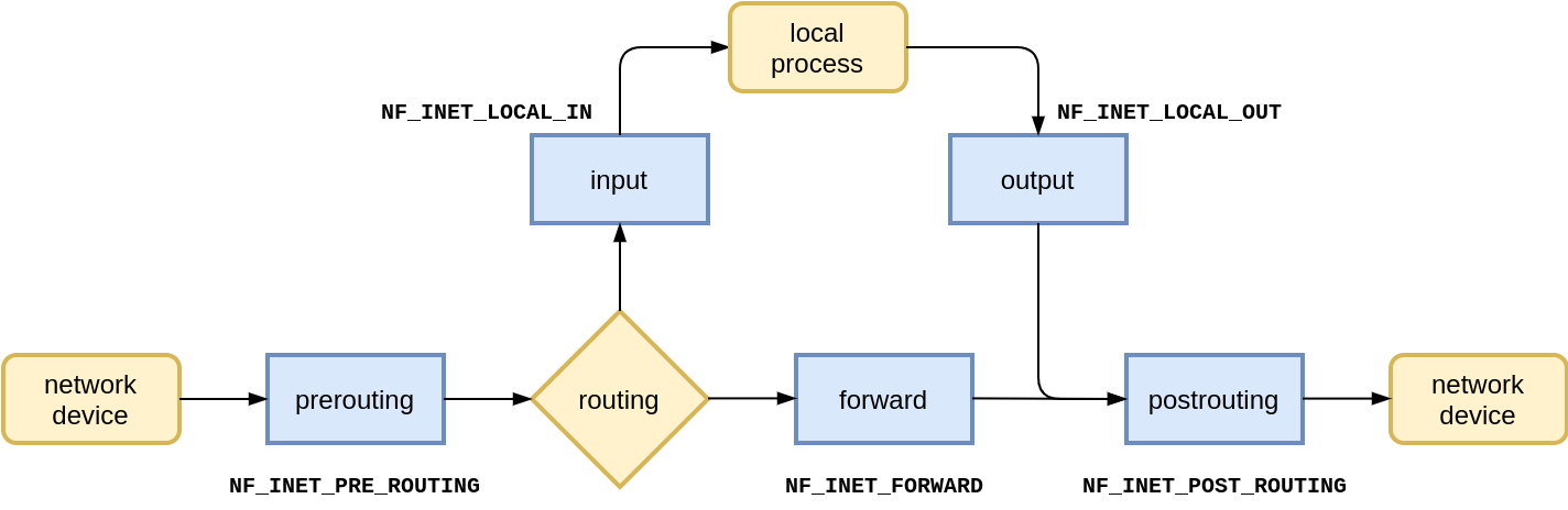
Which ones does conntrack use? We will get to that in a moment.
First, let’s focus on the trigger. What makes conntrack register its callbacks with Netfilter?
The SSH connection doesn’t show up in the conntrack table just because the module is loaded. We already saw that. This means that conntrack doesn’t register its callbacks with Netfilter at module load time.
Or at least, it doesn’t do it by default. Since Linux v5.1 (May 2019) the conntrack module has the enable_hooks parameter, which causes conntrack to register its callbacks on load:
[vagrant@ct-vm ~]$ modinfo nf_conntrack
…
parm:           enable_hooks:Always enable conntrack hooks (bool)
Going back to our toy VM, let’s try to reload the conntrack module with enable_hooks set:
[vagrant@ct-vm ~]$ sudo rmmod nf_conntrack_netlink nf_conntrack
[vagrant@ct-vm ~]$ sudo modprobe nf_conntrack enable_hooks=1
[vagrant@ct-vm ~]$ sudo conntrack -L
tcp      6 431999 ESTABLISHED src=192.168.122.204 dst=192.168.122.1 sport=22 dport=34858 src=192.168.122.1 dst=192.168.122.204 sport=34858 dport=22 [ASSURED] mark=0 secctx=system_u:object_r:unlabeled_t:s0 use=1
conntrack v1.4.5 (conntrack-tools): 1 flow entries have been shown.
[vagrant@ct-vm ~]$
Nice! The conntrack table now contains an entry for our SSH session.
The Netfilter hook notified conntrack about SSH session packets passing through the stack.
Now that we know how conntrack gets called, we can go back to our question — can we observe a TCP SYN packet dropped by the firewall with conntrack?
Listing Netfilter hooks
That is easy to check:
- Add a rule to drop anything coming to port tcp/25702
[vagrant@ct-vm ~]$ sudo iptables -t filter -A INPUT -p tcp --dport 2570 -j DROP
2) Connect to the VM on port tcp/2570 from the outside
host $ nc -w 1 -z 192.168.122.204 2570
3) List conntrack table entries
[vagrant@ct-vm ~]$ sudo conntrack -L
tcp      6 431999 ESTABLISHED src=192.168.122.204 dst=192.168.122.1 sport=22 dport=34858 src=192.168.122.1 dst=192.168.122.204 sport=34858 dport=22 [ASSURED] mark=0 secctx=system_u:object_r:unlabeled_t:s0 use=1
conntrack v1.4.5 (conntrack-tools): 1 flow entries have been shown.
No new entries. Conntrack didn’t record a new flow for the dropped SYN.
But did it process the SYN packet? To answer that we have to find out which callbacks conntrack registered with Netfilter.
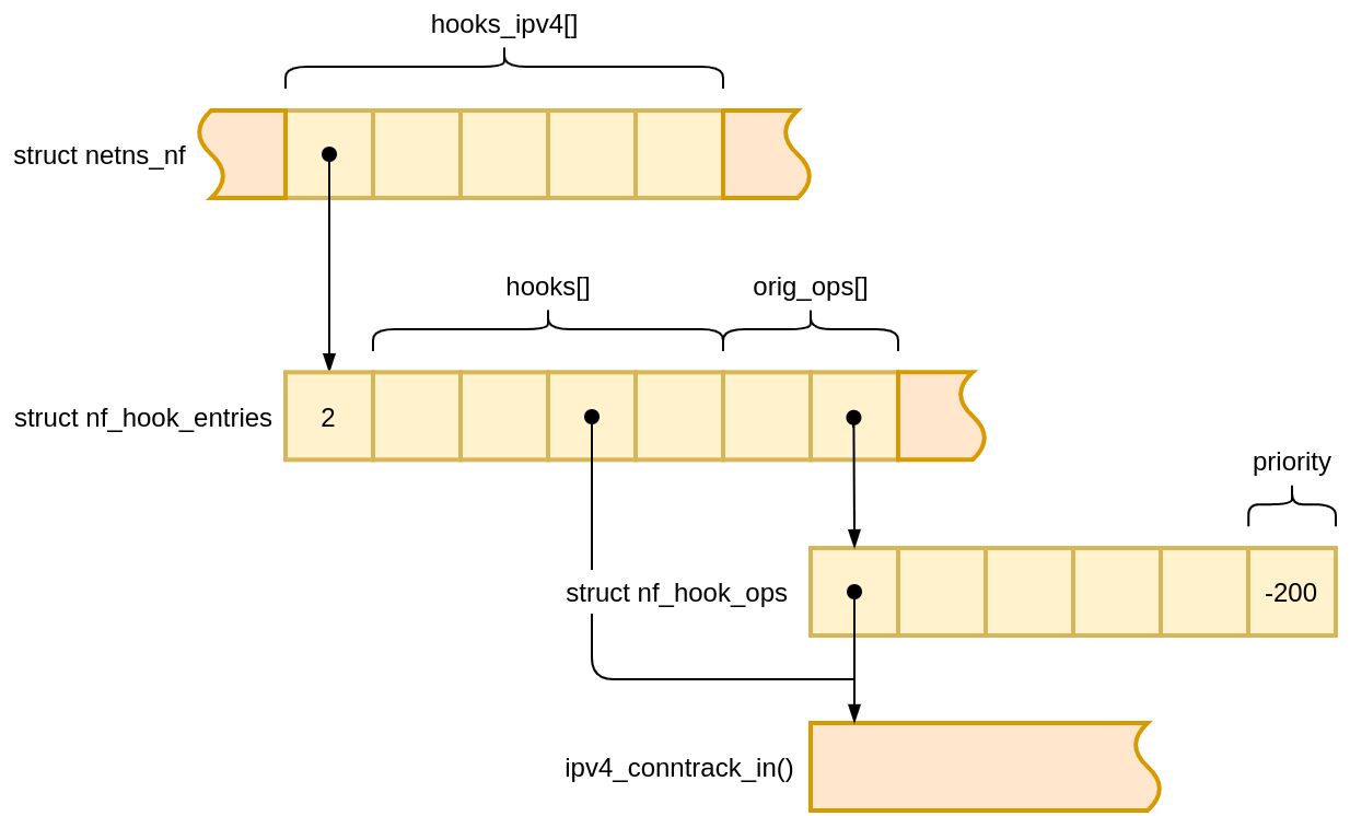
Netfilter keeps track of callbacks registered for each hook in instances of struct nf_hook_entries. We can reach these objects through the Netfilter state (struct netns_nf), which lives inside network namespace (struct net).
struct netns_nf {
    …
    struct nf_hook_entries __rcu *hooks_ipv4[NF_INET_NUMHOOKS];
    struct nf_hook_entries __rcu *hooks_ipv6[NF_INET_NUMHOOKS];
    …
}
struct nf_hook_entries, if you look at its definition, is a bit of an exotic construct. A glance at how the object size is calculated during its allocation gives a hint about its memory layout:
    struct nf_hook_entries *e;
    size_t alloc = sizeof(*e) +
               sizeof(struct nf_hook_entry) * num +
               sizeof(struct nf_hook_ops *) * num +
               sizeof(struct nf_hook_entries_rcu_head);
It’s an element count, followed by two arrays glued together, and some RCU-related state which we’re going to ignore. The two arrays have the same size, but hold different kinds of values.
We can walk the second array, holding pointers to struct nf_hook_ops, to discover the registered callbacks and their priority. Priority determines the invocation order.
With drgn, a programmable C debugger tailored for the Linux kernel, we can locate the Netfilter state in kernel memory, and walk its contents relatively easily. Given we know what we are looking for.
[vagrant@ct-vm ~]$ sudo drgn
drgn 0.0.8 (using Python 3.9.1, without libkdumpfile)
…
>>> pre_routing_hook = prog['init_net'].nf.hooks_ipv4[0]
>>> for i in range(0, pre_routing_hook.num_hook_entries):
...     pre_routing_hook.hooks[i].hook
...
(nf_hookfn *)ipv4_conntrack_defrag+0x0 = 0xffffffffc092c000
(nf_hookfn *)ipv4_conntrack_in+0x0 = 0xffffffffc093f290
>>>
Neat! We have a way to access Netfilter state.
Let’s take it to the next level and list all registered callbacks for each Netfilter hook (using less than 100 lines of Python):
[vagrant@ct-vm ~]$ sudo /vagrant/tools/list-nf-hooks
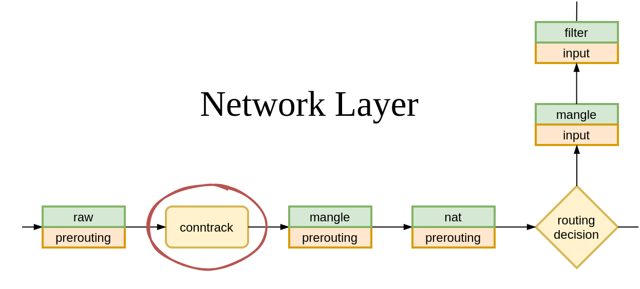
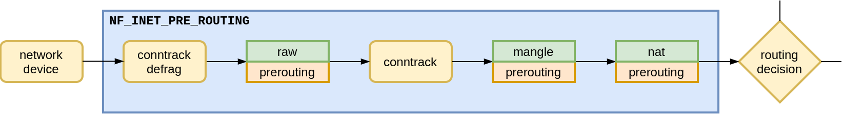
🪝 ipv4 PRE_ROUTING
-400 → ipv4_conntrack_defrag ☜ conntrack callback
-300 → iptable_raw_hook
-200 → ipv4_conntrack_in ☜ conntrack callback
-150 → iptable_mangle_hook
-100 → nf_nat_ipv4_in
🪝 ipv4 LOCAL_IN
-150 → iptable_mangle_hook
0 → iptable_filter_hook
50 → iptable_security_hook
100 → nf_nat_ipv4_fn
2147483647 → ipv4_confirm
…
The output from our script shows that conntrack has two callbacks registered with the PRE_ROUTING hook – ipv4_conntrack_defrag and ipv4_conntrack_in. But are they being called?
Tracing conntrack callbacks
We expect that when the Netfilter PRE_ROUTING hook processes a TCP SYN packet, it will invoke ipv4_conntrack_defrag and then ipv4_conntrack_in callbacks.
To confirm it we will put to use the tracing powers of BPF 🐝. BPF programs can run on entry to functions. These kinds of programs are known as BPF kprobes. In our case we will attach BPF kprobes to conntrack callbacks.
Usually, when working with BPF, we would write the BPF program in C and use clang -target bpf to compile it. However, for tracing it will be much easier to use bpftrace. With bpftrace we can write our BPF kprobe program in a high-level language inspired by AWK:
kprobe:ipv4_conntrack_defrag,
kprobe:ipv4_conntrack_in
{
    $skb = (struct sk_buff *)arg1;
    $iph = (struct iphdr *)($skb->head + $skb->network_header);
    $th = (struct tcphdr *)($skb->head + $skb->transport_header);

    if ($iph->protocol == 6 /* IPPROTO_TCP */ &&
        $th->dest == 2570 /* htons(2570) */ &&
        $th->syn == 1) {
        time("%H:%M:%S ");
        printf("%s:%u > %s:%u tcp syn %s\n",
               ntop($iph->saddr),
               (uint16)($th->source << 8) | ($th->source >> 8),
               ntop($iph->daddr),
               (uint16)($th->dest << 8) | ($th->dest >> 8),
               func);
    }
}
What does this program do? It is roughly an equivalent of a tcpdump filter:
dst port 2570 and tcp[tcpflags] & tcp-syn != 0
But only for packets passing through conntrack PRE_ROUTING callbacks.
(If you haven’t used bpftrace, it comes with an excellent reference guide and gives you the ability to explore kernel data types on the fly with bpftrace -lv 'struct iphdr'.)
Let’s run the tracing program while we connect to the VM from the outside (nc -z 192.168.122.204 2570):
[vagrant@ct-vm ~]$ sudo bpftrace /vagrant/tools/trace-conntrack-prerouting.bt
Attaching 3 probes...
Tracing conntrack prerouting callbacks... Hit Ctrl-C to quit
13:22:56 192.168.122.1:33254 > 192.168.122.204:2570 tcp syn ipv4_conntrack_defrag
13:22:56 192.168.122.1:33254 > 192.168.122.204:2570 tcp syn ipv4_conntrack_in
^C

[vagrant@ct-vm ~]$
Conntrack callbacks have processed the TCP SYN packet destined to tcp/2570.
But if conntrack saw the packet, why is there no corresponding flow entry in the conntrack table?
Going down the rabbit hole
What actually happens inside the conntrack PRE_ROUTING callbacks?
To find out, we can trace the call chain that starts on entry to the conntrack callback. The function_graph tracer built into the Ftrace framework is perfect for this task.
But because all incoming traffic goes through the PRE_ROUTING hook, including our SSH connection, our trace will be polluted with events from SSH traffic. To avoid that, let’s switch from SSH access to a serial console.
When using libvirt as the Vagrant provider, you can connect to the serial console with virsh:
host $ virsh -c qemu:///session list
 Id   Name                State
-----------------------------------
 1    conntrack_default   running

host $ virsh -c qemu:///session console conntrack_default
Once connected to the console and logged into the VM, we can record the call chain using the trace-cmd wrapper for Ftrace:
[vagrant@ct-vm ~]$ sudo trace-cmd start -p function_graph -g ipv4_conntrack_defrag -g ipv4_conntrack_in
  plugin 'function_graph'
[vagrant@ct-vm ~]$ # … connect from the host with `nc -z 192.168.122.204 2570` …
[vagrant@ct-vm ~]$ sudo trace-cmd stop
[vagrant@ct-vm ~]$ sudo cat /sys/kernel/debug/tracing/trace
# tracer: function_graph
#
# CPU  DURATION                  FUNCTION CALLS
# |     |   |                     |   |   |   |
 1)   1.219 us    |  finish_task_switch();
 1)   3.532 us    |  ipv4_conntrack_defrag [nf_defrag_ipv4]();
 1)               |  ipv4_conntrack_in [nf_conntrack]() {
 1)               |    nf_conntrack_in [nf_conntrack]() {
 1)   0.573 us    |      get_l4proto [nf_conntrack]();
 1)               |      nf_ct_get_tuple [nf_conntrack]() {
 1)   0.487 us    |        nf_ct_get_tuple_ports [nf_conntrack]();
 1)   1.564 us    |      }
 1)   0.820 us    |      hash_conntrack_raw [nf_conntrack]();
 1)   1.255 us    |      __nf_conntrack_find_get [nf_conntrack]();
 1)               |      init_conntrack.constprop.0 [nf_conntrack]() {  ❷
 1)   0.427 us    |        nf_ct_invert_tuple [nf_conntrack]();
 1)               |        __nf_conntrack_alloc [nf_conntrack]() {      ❶
                             …
 1)   3.680 us    |        }
                           …
 1) + 15.847 us   |      }
                         …
 1) + 34.595 us   |    }
 1) + 35.742 us   |  }
 …
[vagrant@ct-vm ~]$
What catches our attention here is the allocation, __nf_conntrack_alloc() (❶), inside init_conntrack() (❷). __nf_conntrack_alloc() creates a struct nf_conn object which represents a tracked connection.
This object is not created in vain. A glance at init_conntrack() source shows that it is pushed onto a list of unconfirmed connections3.
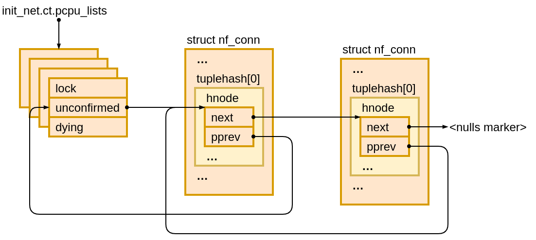
What does it mean that a connection is unconfirmed? As conntrack(8) man page explains:
unconfirmed:
       This table shows new entries, that are not yet inserted into the
       conntrack table. These entries are attached to packets that  are
       traversing  the  stack, but did not reach the confirmation point
       at the postrouting hook.
Perhaps we have been looking for our flow in the wrong table? Does the unconfirmed table have a record for our dropped TCP SYN?
Pulling the rabbit out of the hat
I have bad news…
[vagrant@ct-vm ~]$ sudo conntrack -L unconfirmed
conntrack v1.4.5 (conntrack-tools): 0 flow entries have been shown.
[vagrant@ct-vm ~]$
The flow is not present in the unconfirmed table. We have to dig deeper.
Let’s for a moment assume that a struct nf_conn object was added to the unconfirmed list. If the list is now empty, then the object must have been removed from the list before we inspected its contents.
Has an entry been removed from the unconfirmed table? What function removes entries from the unconfirmed table?
It turns out that nf_ct_add_to_unconfirmed_list() which init_conntrack() invokes, has its opposite defined just right beneath it – nf_ct_del_from_dying_or_unconfirmed_list().
It is worth a shot to check if this function is being called, and if so, from where. For that we can again use a BPF tracing program, attached to function entry. However, this time our program will record a kernel stack trace:
kprobe:nf_ct_del_from_dying_or_unconfirmed_list { @[kstack()] = count(); exit(); }
With bpftrace running our one-liner, we connect to the VM from the host with nc as before:
[vagrant@ct-vm ~]$ sudo bpftrace -e 'kprobe:nf_ct_del_from_dying_or_unconfirmed_list { @[kstack()] = count(); exit(); }'
Attaching 1 probe...

@[
    nf_ct_del_from_dying_or_unconfirmed_list+1 ❹
    destroy_conntrack+78
    nf_conntrack_destroy+26
    skb_release_head_state+78
    kfree_skb+50 ❸
    nf_hook_slow+143 ❷
    ip_local_deliver+152 ❶
    ip_sublist_rcv_finish+87
    ip_sublist_rcv+387
    ip_list_rcv+293
    __netif_receive_skb_list_core+658
    netif_receive_skb_list_internal+444
    napi_complete_done+111
    …
]: 1

[vagrant@ct-vm ~]$
Bingo. The conntrack delete function was called, and the captured stack trace shows that on local delivery path (❶), where LOCAL_IN Netfilter hook runs (❷), the packet is destroyed (❸). Conntrack must be getting called when sk_buff (the packet and its metadata) is destroyed. This causes conntrack to remove the unconfirmed flow entry (❹).
It makes sense. After all we have a DROP rule in the filter/INPUT chain. And that iptables -j DROP rule has a significant side effect. It cleans up an entry in the conntrack unconfirmed table!
This explains why we can’t observe the flow in the unconfirmed table. It lives for only a very short period of time.
Not convinced? You don’t have to take my word for it. I will prove it with a dirty trick!
Making the rabbit disappear, or actually appear
If you recall the output from list-nf-hooks that we’ve seen earlier, there is another conntrack callback there – ipv4_confirm, which I have ignored:
[vagrant@ct-vm ~]$ sudo /vagrant/tools/list-nf-hooks
…
🪝 ipv4 LOCAL_IN
       -150 → iptable_mangle_hook
          0 → iptable_filter_hook
         50 → iptable_security_hook
        100 → nf_nat_ipv4_fn
 2147483647 → ipv4_confirm              ☜ another conntrack callback
…
ipv4_confirm is “the confirmation point” mentioned in the conntrack(8) man page. When a flow gets confirmed, it is moved from the unconfirmed table to the main conntrack table.
The callback is registered with a “weird” priority – 2,147,483,647. It’s the maximum positive value of a 32-bit signed integer can hold, and at the same time, the lowest possible priority a callback can have.
This ensures that the ipv4_confirm callback runs last. We want the flows to graduate from the unconfirmed table to the main conntrack table only once we know the corresponding packet has made it through the firewall.
Luckily for us, it is possible to have more than one callback registered with the same priority. In such cases, the order of registration matters. We can put that to use. Just for educational purposes.
Good old iptables won’t be of much help here. Its Netfilter callbacks have hard-coded priorities which we can’t change. But nftables, the iptables successor, is much more flexible in this regard. With nftables we can create a rule chain with arbitrary priority.
So this time, let’s use nftables to install a filter rule to drop traffic to port tcp/2570. The trick, though, is to register our chain before conntrack registers itself. This way our filter will run last.
First, delete the tcp/2570 drop rule in iptables and unregister conntrack.
vm # iptables -t filter -F
vm # rmmod nf_conntrack_netlink nf_conntrack
Then add tcp/2570 drop rule in nftables, with lowest possible priority.
vm # nft add table ip my_table
vm # nft add chain ip my_table my_input { type filter hook input priority 2147483647 \; }
vm # nft add rule ip my_table my_input tcp dport 2570 counter drop
vm # nft -a list ruleset
table ip my_table { # handle 1
        chain my_input { # handle 1
                type filter hook input priority 2147483647; policy accept;
                tcp dport 2570 counter packets 0 bytes 0 drop # handle 4
        }
}
Finally, re-register conntrack hooks.
vm # modprobe nf_conntrack enable_hooks=1
The registered callbacks for the LOCAL_IN hook now look like this:
vm # /vagrant/tools/list-nf-hooks
…
🪝 ipv4 LOCAL_IN
       -150 → iptable_mangle_hook
          0 → iptable_filter_hook
         50 → iptable_security_hook
        100 → nf_nat_ipv4_fn
 2147483647 → ipv4_confirm, nft_do_chain_ipv4
…
What happens if we connect to port tcp/2570 now?
vm # conntrack -L
tcp      6 115 SYN_SENT src=192.168.122.1 dst=192.168.122.204 sport=54868 dport=2570 [UNREPLIED] src=192.168.122.204 dst=192.168.122.1 sport=2570 dport=54868 mark=0 secctx=system_u:object_r:unlabeled_t:s0 use=1
conntrack v1.4.5 (conntrack-tools): 1 flow entries have been shown.
We have fooled conntrack 💥
Conntrack promoted the flow from the unconfirmed to the main conntrack table despite the fact that the firewall dropped the packet. We can observe it.
Outro
Conntrack processes every received packet4 and creates a flow for it. A flow entry is always created even if the packet is dropped shortly after. The flow might never be promoted to the main conntrack table and can be short lived.
However, this blog post is not really about conntrack. Its internals have been covered by magazines, papers, books, and on other blogs long before. We probably could have learned elsewhere all that has been shown here.
For us, conntrack was really just an excuse to demonstrate various ways to discover the inner workings of the Linux network stack. As good as any other.
Today we have powerful introspection tools like drgn, bpftrace, or Ftrace, and a cross referencer to plow through the source code, at our fingertips. They help us look under the hood of a live operating system and gradually deepen our understanding of its workings.
I have to warn you, though. Once you start digging into the kernel, it is hard to stop…
………..
1Actually since Linux v5.10 (Dec 2020) there is an additional Netfilter hook for the INET family named NF_INET_INGRESS. The new hook type allows users to attach nftables chains to the Traffic Control ingress hook.
2Why did I pick this port number? Because 2570 = 0x0a0a. As we will see later, this saves us the trouble of converting between the network byte order and the host byte order.
3To be precise, there are multiple lists of unconfirmed connections. One per each CPU. This is a common pattern in the kernel. Whenever we want to prevent CPUs from contending for access to a shared state, we give each CPU a private instance of the state.
4Unless we explicitly exclude it from being tracked with iptables -j NOTRACK.


![Diving into /proc/[pid]/mem](https://blog.cloudflare.com/content/images/2020/10/image3-25.png)
![Diving into /proc/[pid]/mem](https://blog.cloudflare.com/content/images/2020/10/image2-27.png)
![Diving into /proc/[pid]/mem](https://blog.cloudflare.com/content/images/2020/10/image1-39.png)


